CAT#C429 TitlePage 8/5/03 10:01 AM Page 1 RISK …khuongnguyen.free.fr/ebooks/Finance Risk - Risk...

CAT#C429_TitlePage 8/5/03 10:01 AM

CHAPMAN & HALL/CRCA CRC Press Company

Boca Raton London New York Washington, D.C.

Translated and edited by Alexei Filinkov

CHAPMAN & HALL/CRCMonographs and Surveys inPure and Applied Mathematics 131

RISK ANALYSIS IN

FINANCE

AND INSURANCE

ALEXANDER MELNIKOV

This book contains information obtained from authentic and highly regarded sources. Reprinted materialis quoted with permission, and sources are indicated. A wide variety of references are listed. Reasonableefforts have been made to publish reliable data and information, but the author and the publisher cannotassume responsibility for the validity of all materials or for the consequences of their use.

Neither this book nor any part may be reproduced or transmitted in any form or by any means, electronicor mechanical, including photocopying, microfilming, and recording, or by any information storage orretrieval system, without prior permission in writing from the publisher.

The consent of CRC Press LLC does not extend to copying for general distribution, for promotion, forcreating new works, or for resale. Specific permission must be obtained in writing from CRC Press LLCfor such copying.

Direct all inquiries to CRC Press LLC, 2000 N.W. Corporate Blvd., Boca Raton, Florida 33431.

Trademark Notice:

Product or corporate names may be trademarks or registered trademarks, and areused only for identification and explanation, without intent to infringe.

Visit the CRC Press Web site at www.crcpress.com

© 2004 by CRC Press LLC

No claim to original U.S. Government worksInternational Standard Book Number 1-58488-429-0

Library of Congress Card Number 2003055407Printed in the United States of America 1 2 3 4 5 6 7 8 9 0

Printed on acid-free paper

Library of Congress Cataloging-in-Publication Data

Melnikov, Alexander.Risk analysis in finance and insurance / Alexander Melnikov

p. cm. (Monographs & surveys in pure & applied math; 131)Includes bibliographical references and index.ISBN 1-58488-429-0 (alk. paper)1. Risk management. 2. Finance. 3. Insurance. I. Title II. Chapman & Hall/CRC

monographs and surveys in pure and applied mathematics ; 131.HD61.M45 2003368—dc21 2003055407

C429-discl Page 1 Friday, August 8, 2003 1:33 PM

http://www.crcpress.com/

To my parents

Ivea and Victor Melnikov

© 2004 CRC Press LLC

Contents

1 Foundations of Financial Risk Management 1.1 Introductory concepts of the securities market. Subject of nancial

mathematics 1.2 Probabilistic foundations of nancial modelling and pricing of con-

tingent claims 1.3 The binomial model of a nancial market. Absence of arbitrage,

uniqueness of a risk-neutral probability measure, martingale repre-sentation.

1.4 Hedging contingent claims in the binomial market model. The Cox-Ross-Rubinstein formula. Forwards and futures.

1.5 Pricing and hedging American options 1.6 Utility functions and St. Petersburg’s paradox. The problem of opti-

mal investment.1.7 The term structure of prices, hedging and investment strategies in the

Ho-Lee model

2 Advanced Analysis of Financial Risks 2.1 Fundamental theorems on arbitrage and completeness. Pricing and

hedging contingent claims in complete and incomplete markets. 2.2 The structure of options prices in incomplete markets and in markets

with constraints. Options-based investment strategies.2.3 Hedging contingent claims in mean square 2.4 Gaussian model of a nancial market and pricing in exible insur-

ance models. Discrete version of the Black-Scholes formula. 2.5 The transition from the binomial model of a nancial market to a

continuous model. The Black-Scholes formula and equation. 2.6 The Black-Scholes model. ‘Greek’ parameters in risk management,

hedging under dividends and budget constraints. Optimal invest-ment.

2.7 Assets with xed income 2.8 Real options: pricing long-term investment projects 2.9 Technical analysis in risk management

3 Insurance Risks. Foundations of Actuarial Analysis 3.1 Modelling risk in insurance and methodologies of premium calcula-

tions



3.2 Probability of bankruptcy as a measure of solvency of an insurancecompany 3.2.1 Cramer-Lundberg model 3.2.2 Mathematical appendix 13.2.3 Mathematical appendix 2 3.2.4 Mathematical appendix 33.2.5 Mathematical appendix 4

3.3 Solvency of an insurance company and investment portfolios 3.3.1 Mathematical appendix 5

3.4 Risks in traditional and innovative methods in life insurance3.5 Reinsurance risks 3.6 Extended analysis of insurance risks in a generalized Cramer-

Lundberg model

A Software Supplement: Computations in Finance and Insurance

B Problems and Solutions B.1 Problems for Chapter 1 B.2 Problems for Chapter 2 B.3 Problems for Chapter 3

C Bibliographic Remark

References

Glossary of Notation


Preface

This book deals with the notion of ‘risk’ and is devoted to analysis of risks in nanceand insurance. More precisely, we study risks associated with future repayments(contingent claims), where we understand risks as uncertainties that may result in nancial loss and affect the ability to make repayments. Our approach to this anal-ysis is based on the development of a methodology for estimating the present valueof the future payments given current nancial, insurance and other information. Us-ing this approach, one can adequately de ne notions of price of a nancial contract,of premium for insurance policy and of reserve of an insurance company. Histor-ically, nancial risks were subject to elementary mathematics of nance and theywere treated separately from insurance risks, which were analyzed in actuarial sci-ence. The development of quantitative methods based on stochastic analysis is akey achievement of modern nancial mathematics. These methods can be naturallyextended and applied in the area of actuarial mathematics, which leads to uni edmethods of risk analysis and management.

The aim of this book is to give an accessible comprehensive introduction to themain ideas, methods and techniques that transform risk management into a quanti-tative science. Because of the interdisciplinary nature of our book, many importantnotions and facts from mathematics, nance and actuarial science are discussed inan appropriately simpli ed manner. Our goal is to present interconnections amongthese disciplines and to encourage our reader to further study of the subject. Weindicate some initial directions in the Bibliographic remark.

The book contains many worked examples and exercises. It represents the contentof the lecture courses ‘Financial Mathematics’, ‘Risk Management’ and ‘ActuarialMathematics’ given by the author at Moscow State University and State University– Higher School of Economics (Moscow, Russia) in 1998-2001, and at University ofAlberta (Edmonton, Canada) in 2002-2003.

This project was partially supported by the following grants: RFBR-00-1596149(Russian Federation), G 227 120201 (University of Alberta, Canada), G 121210913(NSERC, Canada).

The author is grateful to Dr. Alexei Filinkov of the University of Adelaide fortranslating, editing and preparing the manuscript. The author also thanks Dr. Johnvan der Hoek for valuable suggestions, Dr. Andrei Boikov for contributions to Chap-ter 3, and Sergei Schtykov for contributions to the computer supplements.

Alexander Melnikov

Steklov Institute of Mathematics, Moscow, Russia

University of Alberta, Edmonton, Canada


Intro duction

Financial and insurance markets always operate under various types of uncertain-ties that can affect nancial positions of companies and individuals. In nancial andinsurance theories these uncertainties are usually referred to as risks. Given certainstates of the market, and the economy in general, one can talk about risk exposure.Any economic activities of individuals, companies and public establishments aimingfor wealth accumulation assume studying risk exposure. The sequence of the corre-sponding actions over some period of time forms the process of risk management.Some of the main principles and ingredients of risk management are qualitative iden-ti cation of risk; estimation of possible losses; choosing the appropriate strategiesfor avoiding losses and for shifting the risk to other parts of the nancial system,including analysis of the involved costs and using feedback for developing adequatecontrols.

The rst two chapters of the book are devoted to the ( nancial) market risks. Weaim to give an elementary and yet comprehensive introduction to main ideas, meth-ods and (probabilistic) models of nancial mathematics. The probabilistic approachappears to be one of the most ef cient ways of modelling uncertainties in the nan-cial markets. Risks (or uncertainties of nancial market operations) are described interms of statistically stable stochastic experiments and therefore estimation of risksis reduced to construction of nancial forecasts adapted to these experiments. Us-ing conditional expectations, one can quantitatively describe these forecasts giventhe observable market prices (events). Thus, it can be possible to construct dynamichedging strategies and those for optimal investment. The foundations of the modernmethodology of quantitative nancial analysis are the main focus of Chapters 1 and2. Probabilistic methods, rst used in nancial theory in the 1950s, have been devel-oped extensively over the past three decades. The seminal papers in the area werepublished in 1973 by F. Black and M. Scholes [6] and R.C. Merton [32].

In the rst two sections, we introduce the basic notions and concepts of the the-ory of nance and the essential mathematical tools. Sections 1.3-1.7 are devoted tonow-classical binomial model of a nancial market. In the framework of this sim-ple model, we give a clear and accessible introduction to the essential methods usedfor solving the two fundamental problems of nancial mathematics: hedging con-tingent claims and optimal investment. In Section 2.1 we discuss the fundamentaltheorems on arbitrage and completeness of nancial markets. We also describe thegeneral approach to pricing and hedging in complete and incomplete markets, whichgeneralizes methods used in the binomial model. In Section 2.2 we investigate thestructure of option prices in incomplete markets and in markets with constraints.Furthermore, we discuss various options-based investment strategies used in nan-


cial engineering. Section 2.3 is devoted to hedging in the mean square. In Section 2.4we study a discrete Gaussian model of a nancial market, and in particular, we de-rive the discrete version of the celebrated Black-Scholes formula. In Section 2.5 wediscuss the transition from a discrete model of a market to a classical Black-Scholesdiffusion model. We also demonstrate that the Black-Scholes formula (and the equa-tion) can be obtained from the classical Cox-Ross-Rubinstein formula by a limitingprocedure. Section 2.6 contains the rigorous and systematic treatment of the Black-Scholes model, including discussions of perfect hedging, hedging constrained bydividends and budget, and construction of the optimal investment strategy (the Mer-ton’s point) when maximizing the logarithmic utility function. Here we also studya quantile-type strategy for an imperfect hedging under budget constraints. Section2.7 is devoted to continuous term structure models. In Section 2.8 we give an ex-plicit solution of one particular real options problem, that illustrates the potentialof using stochastic analysis for pricing and hedging long-term investment projects.Section 2.9 is concerned with technical analysis in risk management, which is a use-ful qualitative complement to the quantitative risk analysis discussed in the previoussections. This combination of quantitative and qualitative methods constitutes themodern shape of nancial engineering.

Insurance against possible nancial losses is one of the key ingredients of riskmanagement. On the other hand, the insurance business is an integral part of the nancial system. The problems of managing the insurance risks are the focus ofChapter 3. In Sections 3.1 and 3.2 we describe the main approaches used to evaluaterisk in both individual and collective insurance models. Furthermore, in Section 3.3we discuss models that take into account an insurance company’s nancial invest-ment strategies. Section 3.4 is devoted to risks in life insurance; we discuss bothtraditional and innovative exible methods. In Section 3.5 we study risks in rein-surance and, in particular, redistribution of risks between insurance and reinsurancecompanies. It is also shown that for determining the optimal number of reinsur-ance companies one has to use the technique of branching processes. Section 3.6 isdevoted to extended analysis of insurance risks in a generalized Cramer-Lundbergmodel.

The book also offers the Software Supplement: Computations in Finance and In-surance (see Appendix A), which can be downloaded from

www.crcpress.com/e products/downloads/download.asp?cat no = C429

Finally, we note that our treatment of risk management in insurance demonstratesthat methods of risk evaluation and management in insurance and nance are inter-related and can be treated using a single integrated approach. Estimations of futurepayments and of the corresponding risks are the key operational tasks of n ancial andinsurance companies. Management of these risks requires an accurate evaluation ofpresent values of future payments, and therefore adequate modelling of ( nancialand insurance) risk processes. Stochastic analysis is one of the most powerful toolsfor this purpose.


http://www.crcpress.com/e_products/downloads/download.asp?cat_no=C429

Chapter 1

Foundations of Financial RiskManagement

1.1 Introductory concepts of the securities market. Sub-ject of financial mathematics

The notion of an asset (anything of value) is one of the fundamental notions in thefinancial mathematics. Assets can be risky and non-risky. Here risk is understoodas an uncertainty that can cause losses (e.g., of wealth). The most typical represen-tatives of such assets are the following basic securities: stocks S and bonds (bankaccounts) B. These securities constitute the basis of a financial market that can beunderstood as a space equipped with a structure for trading the assets.

Stocks are share securities issued for accumulating capital of a company for itssuccessful operation. The stockholder gets the right to participate in the control ofthe company and to receive dividends. Both depend on the number of shares ownedby the stockholder.

Bonds (debentures) are debt securities issued by a government or a company foraccumulating capital, restructuring debts, etc. In contrast to stocks, bonds are issuedfor a specified period of time. The essential characteristics of a bond include theexercise (redemption) time, face value (redemption cost), coupons (payments up toredemption) and yield (return up to the redemption time). The zero-coupon bond issimilar to a bank account and its yield corresponds to a bank interest rate.

An interest rate r ≥ 0 is typically quoted by banks as an annual percentage.Suppose that a client opens an account with a deposit of B0, then at the end of a1-year period the client’s non-risky profit is ∆B1 = B1 − B0 = rB0. After n yearsthe balance of this account will be Bn = Bn−1 + rB0, given that only the initialdeposit B0 is reinvested every year. In this case r is referred to as a simple interest.

Alternatively, the earned interest can be also reinvested (compounded), then at theend of n years the balance will be Bn = Bn−1(1+ r) = B0(1+ r)n. Note that herethe ratio ∆Bn/Bn−1 reflects the profitability of the investment as it is equal to r, thecompound interest.

Now suppose that interest is compounded m times per year, then

Bn = Bn−1

(1 +

r(m)

m

)m

= B0

(1 +

r(m)

m

)mn

.


Such rate r(m) is quoted as a nominal (annual) interest rate and the equivalent effec-

tive (annual) interest rate is equal to r =(1 + r (m)

m

)m

− 1.

Let t ≥ 0, and consider the ratio

Bt+ 1m− Bt

Bt=

r(m)

m,

where r(m) is a nominal annual rate of interest compounded m times per year. Then

r = limm→∞

Bt+ 1m− Bt

1mBt

= limm→∞ r(m) =

1Bt

dBt

dt

is called the nominal annual rate of interest compounded continuously. Clearly, Bt =B0e

rt.Thus, the concept of interest is one of the essential components in the description

of time evolution of ‘value of money’. Now consider a series of periodic payments(deposits) f0, f1, . . . , fn (annuity). It follows from the formula for compound inter-est that the present value of k-th payment is equal to fk

(1 + r

)−k, and therefore the

present value of the annuity is∑n

k=0 fk

(1 + r

)−k.

WORKED EXAMPLE 1.1Let an initial deposit into a bank account be $10, 000. Given that r(m) = 0.1,find the account balance at the end of 2 years for m = 1, 3 and 6. Also findthe balance at the end of each of years 1 and 2 if the interest is compoundedcontinuously at the rate r = 0.1.

SOLUTION Using the notion of compound interest, we have

B(1)2 = 10, 000

(1 + 0.1

)2

= 12, 100

for interest compounded once per year;

B(3)2 = 10, 000

(1 +

0.13

)2×3

≈ 12, 174

for interest compounded three times per year;

B(6)2 = 10, 000

(1 +

0.16

)2×6

≈ 12, 194

for interest compounded six times per year.For interest compounded continuously we obtain

B(∞)1 = 10, 000 e0.1 ≈ 11, 052 , B

(∞)2 = 10, 000 e2×0.1 ≈ 12, 214 .


Stocks are significantly more volatile than bonds, and therefore they are char-acterized as risky assets. Similarly to bonds, one can define their profitabilityρn = ∆Sn/Sn−1, n = 1, 2, . . ., where Sn is the price of a stock at time n. Then wehave the following discrete equation Sn = Sn−1(1 + ρn), S0 > 0.

The mathematical model of a financial market formed by a bank account B (withan interest rate r) and a stock S (with profitabilities ρn) is referred to as a (B,S)-market.

The volatility of prices Sn is caused by a great variety of sources, some of whichmay not be easily observed. In this case, the notion of randomness appears to beappropriate, so that Sn, and therefore ρn, can be considered as random variables.Since at every time step n the price of a stock goes either up or down, then it is naturalto assume that profitabilities ρn form a sequence of independent random variables(ρn)∞n=1 that take values b and a (b > a) with probabilities p and q respectively(p + q = 1). Next, we can write ρn as a sum of its mean µ = bp + aq and a randomvariable wn = ρn − µ whose expectation is equal to zero. Thus, profitability ρn

can be described in terms of an ‘independent random deviation’ wn from the meanprofitability µ.

When the time steps become smaller, the oscillations of profitability become morechaotic. Formally the ‘limit’ continuous model can be written as

St

St≡ dSt

dt

1St

= µ + σwt ,

where µ is the mean profitability, σ is the volatility of the market and wt is theGaussian white noise.

The formulae for compound and continuous rates of interest together with thecorresponding equation for stock prices, define the binomial (Cox-Ross-Rubinstein)and the diffusion (Black-Scholes) models of the market, respectively.

A participant in a financial market usually invests free capital in various availableassets that then form an investment portfolio. The process of building and managingsuch a portfolio is indeed the management of the capital. The redistribution of aportfolio with the goal of limiting or minimizing the risk in various financial trans-action is usually referred to as hedging. The corresponding portfolio is then calleda hedging portfolio. An investment strategy (portfolio) that may give a profit evenwith zero initial investment is called an arbitrage strategy. The presence of arbitragereflects the instability of a financial market.

The development of a financial market offers the participants the derivative se-curities, i.e., securities that are formed on the basis of the basic securities – stocksand bonds. The derivative securities (forwards, futures, options etc.) require smallerinitial investment and play the role of insurance against possible losses. Also, theyincrease the liquidity of the market.

For example, suppose company A plans to purchase shares of company B at theend of the year. To protect itself from a possible increase in shares prices, companyA reaches an agreement with company B to buy the shares at the end of the year fora fixed (forward) price F . Such an agreement between the two companies is called aforward contract (or simply, forward).


Now suppose that company A plans to sell some shares to company B at the endof the year. To protect itself from a possible fall in price of those shares, companyA buys a put option (seller’s option), which confers the right to sell the shares at theend of the year at the fixed strike price K. Note that in contrast to the forwards case,a holder of an option must pay a premium to its issuer.

Futures contract is an agreement similar to the forward contract but the tradingtakes place on a stock exchange, a special organization that manages the trading ofvarious goods, financial instruments and services.

Finally, we reiterate here that mathematical models of financial markets, method-ologies for pricing various financial instruments and for constructing optimal (mini-mizing risk) investment strategies are all subject to modern financial mathematics.

1.2 Probabilistic foundations of financial modelling andpricing of contingent claims

Suppose that a non-risky asset B and a risky asset S are completely described atany time n = 0, 1, 2, . . . by their prices. Therefore, it is natural to assume that theprice dynamics of these securities is the essential component of a financial market.These dynamics are represented by the following equations

∆Bn = rBn−1 , B0 = 1 ,

∆Sn = ρnSn−1 , S0 > 0 ,

where ∆Bn = Bn−Bn−1 , ∆Sn = Sn−Sn−1 , n = 1, 2, . . . ; r ≥ 0 is a constantrate of interest and ρn will be specified later in this section.

Another important component of a financial market is the set of admissible ac-tions or strategies that are allowed in dealing with assets B and S. A sequenceπ = (πn)∞n=1 ≡ (βn, γn)∞n=1 is called an investment strategy (portfolio) if for anyn = 1, 2, . . . the quantities βn and γn are determined by prices S1, . . . Sn−1. Inother words, βn = βn(S1, . . . Sn−1) and γn = γn(S1, . . . Sn−1) are functions ofS1, . . . Sn−1 and they are interpreted as the amounts of assets B and S, respectively,at time n. The value of a portfolio π is

Xπn = βnBn + γnSn ,

where βnBn represents the part of the capital deposited in a bank account and γnSn

represents the investment in shares. If the value of a portfolio can change only dueto changes in assets prices: ∆Xπ

n = Xπn − Xπ

n−1 = βn∆Bn + γn∆Sn , then π issaid to be a self-financing portfolio. The class of all such portfolios is denoted SF .

A common feature of all derivative securities in a (B,S)-market is their poten-tial liability (payoff) fN at a future time N . For example, for forwards we havefN = SN − F and for call options fN = (SN − K)+ ≡ maxSN − K, 0. Such


liabilities inherent in derivative securities are called contingent claims. One of themost important problems in the theory of contingent claims is their pricing at anytime before the expiry date N . This problem is related to the problem of hedgingcontingent claims. A self-financing portfolio is called a hedge for a contingent claimfN if Xπ

n ≥ fN for any behavior of the market. If a hedging portfolio is not unique,then it is important to find a hedge π∗ with the minimum value: Xπ∗

n ≤ Xπn for

any other hedge π. Hedge π∗ is called the minimal hedge. The minimal hedge givesan obvious solution to the problem of pricing a contingent claim: the fair price ofthe claim is equal to the value of the minimal hedging portfolio. Furthermore, theminimal hedge manages the risk inherent in a contingent claim.

Next we introduce some basic notions from probability theory and stochastic anal-ysis that are helpful in studying risky assets. We start with the fundamental notion ofan ‘experiment’ when the set of possible outcomes of the experiment is known butit is not known a priori which of those outcomes will take place (this constitutes therandomness of the experiment).

Example 1.1 (Trading on a stock exchange)A set of possible exchange rates between the dollar and the euro is alwaysknown before the beginning of trading, but not the exact value.

Let Ω be the set of all elementary outcomes ω and let F be the set of all events(non-elementary outcomes), which contains the impossible event ∅ and the certainevent Ω.

Next, suppose that after repeating an experiment n times, an event A ∈ F occurrednA times. Let us consider experiments whose ‘randomness’ possesses the followingproperty of statistical stability: for any event A there is a number P (A) ∈ [0, 1] suchthat nA/n → P (A) as n → ∞. This number P (A) is called the probability of eventA. Probability P : F → [0, 1] is a function with the following properties:

1. P (Ω) = 1 and P (∅) = 0;

2. P( ∪k Ak

)=∑

k P (Ak) for Ai ∩ Aj = ∅.

The triple (Ω,F , P ) is called a probability space. Every event A ∈ F can beassociated with its indicator:

IA(ω) =1 , if ω ∈ A0 , if ω ∈ Ω \ A

.

Any measurable function X : Ω → R is called a random variable. An indicator isan important simplest example of a random variable. A random variable X is calleddiscrete if the range of function X(·) is countable: (xk)∞k=1. In this case we have thefollowing representation

X(ω) =∞∑

k=1

xkIAk(ω) ,


where Ak ∈ F and ∪kAk = Ω. A discrete random variable X is called simple if thecorresponding sum is finite. The function

FX(x) := P (ω : X ≤ x) , x ∈ R

is called the distribution function of X . For a discrete X we have

FX(x) =∑

k:xk≤x

P (ω : X = xk) ≡∑

k:xk≤x

pk .

The sequence (pk)∞k=1 is called the probability distribution of a discrete randomvariable X . If function FX(·) is continuous on R , then the corresponding randomvariable X is said to be continuous. If there exists a non-negative function p(·) suchthat

FX(x) =∫ x

−∞p(y)dy ,

then X is called an absolutely continuous random variable and p is its density. Theexpectation (or mean value) of X in these cases is

E(X) =∑k≥1

xkpk

and

E(X) =∫

R

xp(x)dx ,

respectively. Given a random variable X , for most functions g : R → R it is possibleto define a random variable Y = g(X) with expectation

E(Y ) =∑k≥1

g(xk)pk

in the discrete case and

E(Y ) =∫

R

g(x)p(x)dx

for a continuous Y . In particular, the quantity

V (X) = E[(

X − E(X))2]

is called the variance of X .

Example 1.2 (Examples of discrete probability distributions)

1. Bernoulli:

p0 = P (ω : X = a) = p , p1 = P (ω : X = b) = 1− p ,

where p ∈ [0, 1] and a, b ∈ R.


2. Binomial:

pm = P (ω : X = m) =(

nk

)pm(1− p)n−m ,

where p ∈ [0, 1], n ≥ 1 and m = 0, 1, . . . , n.

3. Poisson (with parameter λ > 0):

pm = P (ω : X = m) = e−λ λm

m!

for m = 0, 1, . . . .

One of the most important examples of an absolutely continuous random variableis a Gaussian (or normal) random variable with the density

p(x) =1√2πσ

e−(x−m)2

2σ2 , x,m ∈ R , σ > 0 ,

where m = E(X) is its mean value and σ2 = V (X) is its variance. In this case oneusually writes X = N (m,σ2).

Consider a positive random variable Z on a probability space (Ω,F , P ). Supposethat E(Z) = 1, then for any event A ∈ F define its new probability

P (A) = E(ZIA) . (1.1)

The expectation of a random variable X with respect to this new probability is

E(X) =∑

k

xkP(ω : X = xk

)=∑

k

xkE(Z Iω: X=xk

)=∑

k

E(Z xk Iω: X=xk

)= E

(Z∑

k

xk Iω: X=xk)

= E(ZX) .

The proof of this formula is based on the following simple observation

E

( n∑i=1

ciXi

)=

n∑i=1

ciE(Xi)

for real constants ci. Random variable Z is called the density of the probability Pwith respect to P .

For the sake of simplicity, in the following discussion we restrict ourselves tothe case of discrete random variables X and Y with values (xi)∞i=1 and (yi)∞i=1

respectively. The probabilities

P(ω : X = xi, Y = yi

) ≡ pij , pij ≥ 0,∑i,j

pij = 1,


form the joint distribution of X and Y . Denote pi =∑

j pij and pj =∑

i pij , thenrandom variables X and Y are called independent if pij = pi ·pj , which implies thatE(XY ) = E(X)E(Y ).

The quantity

E(X|Y = yi) :=∑

i

xipij

pj

is called the conditional expectation of X with respect to Y = yi. The randomvariable E(X|Y ) is called the conditional expectation of X with respect to Y ifE(X|Y ) is equal to E(X|Y = yi) on every set ω : Y = yi. In particular, forindicators X = IA and Y = IB we obtain

E(X|Y ) = P (A|B) =P (AB)P (B)

.

We mention some properties of conditional expectations:

1. E(X) = E(E(X|Y )

), in particular, for X = IA and Y = IB we have

P (A) = P (B)P (A|B) + P (Ω \ B)P (A|Ω \ B);

2. if X and Y are independent, then E(X|Y ) = E(X);

3. since by the definition E(X|Y ) is a function of Y , then conditional expecta-tion can be interpreted as a prediction of X given the information from the‘observed’ random variable Y .

Finally, for a random variable X with values in 0, 1, 2, . . . we introduce thenotion of a generating function

φX(x) = E(zX) =∑

i

zipi .

We have

φ(1) = 1 ,dkφ

dxk

∣∣∣x=0

= k!pk

and

φX1+···+Xk(x) =

k∏i=1

φXi(x)

for independent random variables X1, . . . , Xk.

Example 1.3 (Trading on a stock exchange: Revisited)Consider the following time scale: n = 0 (present time), . . . , n = N (can beone month, quarter, year etc.).An elementary outcome can be written in the form of a sequence ω =

(ω1, . . . , ωN ), where ωi is an elementary outcome representing the results oftrading at time step i = 1, . . . , N . Now we consider a probability space


(Ω,FN , P ) that contains all trading results up to time N . For any n ≤ N wealso introduce the corresponding probability space (Ω,Fn, P ) with elementaryoutcomes (ω1, . . . , ωn) ∈ Fn ⊆ FN .Thus, to describe evolution of trading on a stock exchange we need a filtered

probability space (Ω,FN , F, P ) called a stochastic basis, where F = (Fn)n≤N

is called a filtration (or information flow):

F0 = ∅,Ω ⊆ F1 ⊆ . . . ⊆ FN .

For technical reasons, it is convenient to assume that if A ∈ Fn ∈ F, thenFn also contains the complement of A and is closed under taking countableunions and intersections, that is Fn is a σ-algebra.

Now consider a (B,S)-market. Since asset B is non-risky, we can assume thatB(ω) ≡ Bn for all ω ∈ Ω. For a risky asset S it is natural to assume that pricesS1, . . . , SN are random variables on the stochastic basis (Ω,FN , F, P ). Each ofSn is completely determined by the trading results up to time n ≤ N or in otherwords, by the σ-algebra of events Fn. We also assume that the sources of tradingrandomness are exhausted by the stock prices, i.e. Fn = σ(S1, . . . , Sn) is a σ-algebra generated by random variables S1, . . . , Sn.

Let us consider a specific example of a (B,S)-market. Let ρ1, . . . , ρN be in-dependent random variables taking values a and b (a < b) with probabilitiesP (ω : ρk = b) = p and P (ω : ρk = a) = 1 − p ≡ q. Define the prob-ability basis: Ω = a, bN is the space of sequences of length N whose elementsare equal to either a or b; F = 2Ω is the set of all subsets of Ω. The filtration F isgenerated by the prices (Sn) or equivalently by the sequence (ρn):

Fn = σ(S1, . . . , Sn) = σ(ρ1, . . . , ρn) ,

which means that every random variable on the probability space (Ω,Fn, P ) is afunction of S1, . . . , Sn or, equivalently, of ρ1, . . . , ρn due to relations

∆Sk

Sk−1− 1 = ρk , k = 0, 1, . . . .

A financial (B,S)-market defined on this stochastic basis is called binomial.Consider a contingent claim fN . Since its repayment day is N , then in general,

fN = f(S1, . . . , SN ) is a function of all ‘history’ S1, . . . , SN . The key problemnow is to estimate (or predict) fN at any time n ≤ N given the available marketinformation Fn. We would like these predictions E(fN |Fn) , n = 0, 1, . . . , N , tohave the following intuitively natural properties:

1. E(fN |Fn) is a function of S1, . . . , Sn, but not of future prices Sn+1, . . . , SN .

2. A prediction based on the trivial information F0 = ∅,Ω should coincidewith the mean value of a contingent claim: E(fN |F0) = E(fN ).


3. Predictions must be compatible:

E(fN |Fn) = E(E(fN |Fn+1)

∣∣∣Fn

),

in particular

E(E(fN |Fn)

)= E

(E(fN |Fn)

∣∣∣F0

)= E(fN ) .

4. A prediction based on all possible information FN should coincide with thecontingent claim : E(fN |FN ) = fN .

5. Linearity:

E(φfN + ψgN |Fn) = φE(fN |Fn) + ψE(gN |Fn)

for φ and ψ defined by the information in Fn.

6. If fN does not depend on the information in Fn, then a prediction based onthis information should coincide with the mean value

E(fN |Fn) = E(fN ) .

7. Denote fn = E(fN |Fn), then from property 3 we obtain

E(fn+1|Fn) = E(E(fN |Fn+1)

∣∣∣Fn

)= E(fN |Fn) = fn

for all n ≤ N . Such stochastic sequences are called martingales.

How to calculate predictions? Comparing the notions of a conditional expectationand a prediction, we see that a prediction of fN based on Fn = σ(S1, . . . , Sn) isequal to the conditional expectation of a random variable fN with respect to randomvariables S1, . . . , Sn.

WORKED EXAMPLE 1.2Suppose that the monthly price evolution of stock S is given by

Sn = Sn−1(1 + ρn) , n = 1, 2, . . . ,

where profitabilities ρn are independent random variables taking values 0.2and −0.1 with probabilities 0.4 and 0.6 respectively. Given that the currentprice S0 = 200 ($), find the predicted mean price of S for the next two months.

SOLUTION Since

E(ρ1) = E(ρ2) = 0.2 · 0.4− 0.1 · 0.6 = 0.02 ,


then

E

(S1 + S2

2

∣∣∣∣S0 = 200)= E

(S0(1 + ρ1) + S0(1 + ρ1)(1 + ρ2)

2

∣∣∣∣S0 = 200)

=S0

2

[E(1 + ρ1) + E(1 + ρ1)E(1 + ρ2)

]= 100

[1.02 + 1.02 · 1.02] = 206.4 ($) .

We finish this section with some further notions and facts from stochastic analysis.Let (Ω,F , F, P ) be a stochastic basis. For simplicity we assume that Ω is finite.Consider a stochastic sequence X = (Xn,Fn)n≥0 adopted to filtration F and suchthat E(|Xn|) < ∞ for all n. If

E(Xn|Fn−1) = Xn−1 a.s.

for all n ≥ 1, then X is called a martingale. If

E(Xn|Fn−1) ≥ Xn−1 a.s. or E(Xn|Fn−1) ≤ Xn−1 a.s.

for all n ≥ 1, then X is called a submartingale or a supermartingale, respectively.Let a positive random variable Z be the density of the probability P (see

(1.1)) with respect to P . Consider both these probabilities on measurable spaces(Ω,Fn), n ≥ 0, and denote the corresponding densities Zn. Then Zn = E(Z|Fn)gives an important example of a martingale.

Any supermartingale X admits the Doob decomposition

Xn = Mn − An ,

where M is a martingale and A is a non-decreasing (∆An = An − An−1 ≥ 0)(predictable) stochastic sequence such that A0 = 0 and An is completely determinedby Fn−1.This follows from the following observation

∆Xn = ∆Mn −∆An =[Xn − E(Xn|Fn−1)

]+[E(Xn|Fn−1)− Xn−1

].

Since M2 is a submartingale, then using Doob decomposition we have

M2n = mn + 〈M,M〉n ,

where m is a martingale and 〈M,M〉 is a predictable increasing sequence called thequadratic variation of M . We clearly have

〈M,M〉n =n∑

k=1

E((∆Mk)2

∣∣Fk−1

)and

E(M2

n

)= E

(〈M,M〉n).


For square-integrable martingales M and N one can define their covariance

〈M,N〉n =14

〈M + N,M + N〉n − 〈M − N,M − N〉n

.

Martingales M and N are said to be orthogonal if 〈M,N〉n = 0 or, equivalently, iftheir product M N is a martingale.

Let M be a martingale and H be a predictable stochastic sequence. Then thequantity

H ∗ mn =n∑

k=0

Hk∆mk

is called a discrete stochastic integral. Note that

〈H ∗ m,H ∗ m〉n =n∑

k=0

H2k∆〈m,m〉k .

Consider a stochastic sequence U = (Un)n≥0 with U0 = 0. Define new stochasticsequence X by

∆Xn = Xn−1∆Un , X0 = 1 .

This simple linear stochastic difference equation has an obvious solution

Xn =n∏

k=1

(1 + ∆Uk

)= εn(U) ,

which is called a stochastic exponential.If X is defined by a non-homogeneous equation

∆Xn = ∆Nn + Xn−1∆Un , X0 = N0 ,

then it has the form

Xn = εn(U)

[N0 +

n∑k=1

∆Nk

εk(U)

].

Stochastic exponentials have the following useful properties:

1.1

εn(U)= εn(−U∗) ,

where

∆U∗ =∆Un

1 + ∆Un;

2. ε(U) is a martingale if and only if U is a martingale;

3. εn(U) = 0 for all n ≥ τ0 := infk : εk(U) = 0 ;


4.εn(U)εn(V ) = εn(U + V + [U, V ]) ,

where

[U, V ]n =n∑

k=1

∆Uk∆Vk

is the multiplication rule.

1.3 The binomial model of a financial market. Absenceof arbitrage, uniqueness of a risk-neutral probabilitymeasure, martingale representation.

The binomial model of a (B,S)-market was introduced in the previous section.Sometimes this model is also referred to as the Cox-Ross-Rubinstein model. Recallthat the dynamics of the market are represented by equations

∆Bn = rBn−1 , B0 = 1 ,

∆Sn = ρnSn−1 , S0 > 0 ,

where r ≥ 0 is a constant rate of interest with −1 < a < r < b, and profitabilities

ρn =

b with probability p ∈ [0, 1]a with probability q = 1− p

, n = 1, . . . , N ,

form a sequence of independent identically distributed random variables. Thestochastic basis in this model consists of Ω = a, bN , the space of sequencesx = (x1, . . . , xN ) of length N whose elements are equal to either a or b; F = 2Ω,the set of all subsets of Ω. The probability P has Bernoulli probability distributionwith p ∈ [0, 1], so that

P(x) = p

∑Ni=1 Ib(xi) (1− p)

∑Ni=1 Ia(xi) .

The filtration F is generated by the sequence (ρn)n≤N : Fn = σ(ρ1, . . . , ρn).In the framework of this model we can specify the following notions. A pre-

dictable sequence π = (πn)n≤N ≡ (βn, γn)n≤N is an investment strategy (portfo-lio). A contingent claim fN is a random variable on the stochastic basis (Ω,F , F, P ).Hedge for a contingent claim fN is a self-financing portfolio with the terminal valueXπ

n ≥ fN . A hedge π∗ with the value Xπ∗n ≤ Xπ

n for any other hedge π, is called theminimal hedge. A self-financing portfolio π ∈ SF is called an arbitrage portfolio if

Xπ0 = 0 , Xπ

N ≥ 0 and P(ω : Xπ

N > 0) > 0 ,

which can be interpreted as an opportunity of making a profit without risk.


Note that the risky nature of a (B,S)-market is associated with randomness ofprices Sn. A particular choice of probability P (in terms of Bernoulli parameter p)allows one to numerically express this randomness. In general, the initial choice ofP can give probabilistic properties of S such that the behavior of S is very differentfrom the behavior of a non-risky asset B. On the other hand, it is clear that pricingof contingent claims should be neutral to risk. This can be achieved by introducinga new probability P ∗ such that the behaviors of S and B are similar under thisprobability: S and B are on average the same under P ∗. In other words, the sequenceof discounted prices (Sn/Bn)n≤N must be, on average, constant with respect toprobability P ∗:

E∗(

Sn

Bn

)= E∗

(S0

B0

)= S0 for all n = 1, . . . , N .

For n = 1 this implies

E∗(

S1

B1

)= S0 E∗

(1 + ρ1

1 + r

)= S0

[(1 + b)p∗ + (1 + a)(1− p∗)

]= S0 ,

where p∗ is a Bernoulli parameter that defines P ∗. We have

p∗ + bp∗ + 1 + a − p∗ − ap∗ = 1 + r

and therefore

p∗ =r − a

b − a,

which means that in the binomial model the risk-neutral probability P ∗ is unique,and

P ∗(x) = (p∗)∑N

i=1 Ib(xi) (1− p∗)∑N

i=1 Ia(xi) .

Note that in this case we can find density Z∗N of probability P ∗ with respect to

probability P , i.e. a non-negative random variable such that

E(Z∗

N

)= 1 and P ∗(A) = E

(Z∗

N IA

)for all A ∈ FN .

Since Ω is discrete, we only need to compute values of Z∗N for every elementary

event x. We have

P ∗(x) = E(Z∗

N Ix)= Z∗

N (x)P(x) ,

and hence

Z∗N (x) =

P ∗(x)P(x) =

(p∗

p

)∑Ni=1 Ib(xi)(1− p∗

1− p

)N−∑Ni=1 Ib(xi)

.


To describe the behavior of discounted prices Sn/Bn under the risk-neutral prob-ability P ∗, we compute the following conditional expectations for all n ≤ N :

E∗(

Sn

Bn

∣∣∣∣Fn−1

)= E∗

(S0

n∏k=1

1 + ρk

1 + r

∣∣∣∣Fn−1

)

=S0

1 + rn E∗( n∏

k=1

(1 + ρk)∣∣Fn−1

)

=S0

1 + rn

n−1∏k=1

(1 + ρk)E∗(1 + ρn)

=Sn−1

Bn−1

E∗(1 + ρn)1 + r

=Sn−1

Bn−1

1 + r

1 + r

=Sn−1

Bn−1.

This means that the sequence (Sn/Bn)n≤N is a martingale with respect to the risk-neutral probability P ∗. This is the reason that P ∗ is also referred to as a martingaleprobability (martingale measure).

The next important property of a binomial market is the absence of arbitrage strate-gies. Such a market is referred to as a no-arbitrage market. Consider a self-financingstrategy π = (πn)n≤N ≡ (βn, γn)n≤N ∈ SF with discounted values Xπ

n/Bn. Us-ing properties of martingale probability, we have that for all n ≤ N

E∗(

Xπn

Bn

∣∣∣∣Fn−1

)= E∗

(βn + γn

Sn

Bn

∣∣∣∣Fn−1

)= E∗(βn|Fn−1

)+ γn E∗

(Sn

Bn

∣∣∣∣Fn−1

)= βn + γn

Sn−1

Bn−1=

βnBn−1 + γnSn−1

Bn−1

=Xπ

n−1

Bn−1,

which implies that the discounted value of a self-financing strategy is a martingalewith respect to the risk-neutral probability P ∗. This property is usually referred toas the martingale characterization of self-financing strategies SF .

Further, suppose there exists an arbitrage strategy π. From its definition we have

E

(X π

N

BN

)=

E(X πN )

BN> 0 .

On the other hand, the martingale property of Xπn/Bn implies

E∗(

X πN

BN

)= E∗

(X π

0

B0

)= E∗(X π

0 ) = 0 .


Now, for probabilities P and P ∗ there is a positive density Z∗ so that P ∗(A) =E(Z∗

NIA) for any event A ∈ FN . Therefore

0 = X π0 = X π

0 /B0 = E∗(

X πN

BN

)=

E∗(X πN )

BN=

E(Z∗NX π

N )BN

≥ minω

[Z∗

N (ω)]E(X π

N )BN

> 0 ,

which contradicts the assumption of arbitrage.Now we prove that, in the binomial market framework, any martingale can be rep-

resented in the form of a discrete stochastic integral with respect to some basic mar-tingale. Let (ρn)n≤N be a sequence of independent random variables on (Ω,F , P ∗)defined by

ρn =

a with probability p∗ = r−ab−a

b with probability q∗ = 1− p∗,

where −1 < a < r < b. Consider filtration F generated by the sequence (ρn) :Fn = σ(ρ1, . . . , ρn) . Any martingale (Mn)n≤N , M0 = 0, can be written in theform

Mn =n∑

k=1

φk∆mk , (1.2)

where (φn)n≤N is predictable sequence, and( n∑k=1

∆mk

)n≤N

=( n∑

k=1

(ρk − r))

n≤N

is a (‘Bernoulli’) martingale.Since σ-algebras Fn are generated by ρ1, . . . , ρn, and Mn are completely deter-

mined by Fn, then there exist functions fn = fn(x1, . . . , xn) with xk equal to eithera or b, such that

Mn(ω) = fn(ρ1(ω), . . . , ρn(ω)) , n ≤ N .

The required representation (1.2) can be rewritten in the form

∆Mn(ω) = φk(ω)∆mk

or

fn(ρ1(ω), . . . , ρn−1(ω), b)− fn−1(ρ1(ω), . . . , ρn−1(ω)) = φn(ω)(b − r) ,

fn(ρ1(ω), . . . , ρn−1(ω), a)− fn−1(ρ1(ω), . . . , ρn−1(ω)) = φn(ω)(a − r) ,


and therefore

φn(ω) =fn(ρ1(ω), . . . , ρn−1(ω), b)− fn−1(ρ1(ω), . . . , ρn−1(ω))

(b − r)

=fn(ρ1(ω), . . . , ρn−1(ω), a)− fn−1(ρ1(ω), . . . , ρn−1(ω))

(a − r),

which we now establish. The martingale property implies

E∗(fn(ρ1, . . . , ρn)− fn−1(ρ1, . . . , ρn−1)

∣∣∣Fn−1

)= 0 ,

or

p∗fn(ρ1, . . . , ρn−1, b)− (1− p∗)fn(ρ1, . . . , ρn−1, a) = fn−1(ρ1, . . . , ρn−1) .

Therefore

fn(ρ1(ω), . . . , ρn−1(ω), b)− fn−1(ρ1(ω), . . . , ρn−1(ω))1− p∗

=fn(ρ1(ω), . . . , ρn−1(ω), a)− fn−1(ρ1(ω), . . . , ρn−1(ω))

p∗,

which in view of the choice p∗ = (r − a)/(b − a) proves the result.Using the established martingale representation we now can prove the following

representation for density Z∗N of the martingale probability P ∗ with respect to P :

Z∗N =

N∏k=1

(1− µ − r

σ2(ρk − µ)

)= εN

(− µ − r

σ2

N∑k=1

(ρk − µ))

,

where µ = E(ρk) , σ2 = V (ρk) , k = 1, . . . , N .Indeed, consider Z∗

n = E(Z∗

N

∣∣Fn

), n = 0, 1, . . . , N . From the properties of

conditional expectations we have that (Z∗n)n≤N is a martingale with respect to prob-

ability P and filtration Fn = σ(ρ1, . . . , ρn). Therefore, Z∗n can be written in the

form

Z∗n = 1 +

n∑k=1

(ρk − µ)φk ,

where φk is a predictable sequence. Since Z∗n > 0, we have that it satisfies the

following stochastic equation

Z∗n = 1 +

n∑k=1

Z∗k−1

φk

Z∗k−1

(ρk − µ)

= 1 +n∑

k=1

Z∗k−1 ψk (ρk − µ) ,


and hence

Z∗n =

n∏k=1

(1 + ψk (ρk − µ)

).

Taking into account that Z∗N is the density of a martingale probability, we can com-

pute the coefficients ψk = φk/Z∗k−1. For N = 1 we have

0 = E∗((ρ1 − r)∣∣F0

)= E∗(ρ1 − r) = E

(Z∗

1 (ρ1 − r))

= E((1 + ψ1 (ρ1 − µ)

)(ρ1 − r)

)= (µ − r) + ψ1σ

2 ,

thus ψ1 = −(µ − r)/σ2 .Now suppose that ψk = −(µ − r)/σ2 for all k = 1, . . . , N − 1, then using

independence of ρ1, . . . , ρN we obtain

0 = E∗((ρN − r)∣∣FN−1

)=

E(Z∗

N (ρN − r)∣∣FN−1

)Z∗

N−1

= E((1 + ψN (ρN − µ)

)(ρN − r)

∣∣FN−1

)= E

((ρN − r) + ψN (ρN − µ)(ρN − r)

∣∣FN−1

)= E(ρN − r) + ψN E

((ρN − µ)(ρN − r)

∣∣FN−1

)= (µ − r) + ψNσ2 ,

which gives ψN = −(µ − r)/σ2 and proves the claim.

1.4 Hedging contingent claims in the binomial marketmodel. The Cox-Ross-Rubinstein formula. For-wards and futures.

In the framework of a binomial (B,S)-market we consider a financial contractassociated with a contingent claim fN with the future repayment date N .

If fN is deterministic, then its market risk can be trivially computed sinceE(fN |FN ) ≡ fN . In fact, there is no risk associated with the repayment of thisclaim as one can easily find the present value of the discounted claim fN/BN .

If fN depends on the behavior of the market during the contract period [0, N ],then it is a random variable. The intrinsic risk in this case is related to the ability torepay fN . To estimate and manage this risk, one should be able to predict fN giventhe current market information Fn , n ≤ N .

We start the discussion of a methodology of pricing contingent claims with twosimple examples that illustrate the essence of hedging.


WORKED EXAMPLE 1.3Let Ω = ω1, ω2 and F0 = ∅,Ω , F1 =

∅, ω1, ω2,Ω

. Consider

a single-period binomial (B,S)-market with B0 = 1 ($), S0 = 100 ($), B1 =B0(1+r) = 1+r = 1.2 ($) assuming that the annual rate of interest is r = 0.2,and

S1 =150 ($) with probability p = 0.470 ($) with probability 1− p = 0.6 .

Find the price for a European call option f1 = (S1−K)+ ≡ max0, S1−K ($)with strike price K = 100 ($).

SOLUTION Clearly

f1 = (S1 − 100)+ ≡ max0, S1 − 100 =50 ($) with probability 0.40 ($) with probability 0.6 .

The intuitive price for this option is

E

(f1

1 + r

)=

0.4× 501.2

= 16 .

Now, using the minimal hedging approach to pricing, we construct a self-financing strategy π0 = (β0, γ0) that replicates the final value of the option:Xπ

1 = f1. Since Xπ1 = β0(1 + r) + γ0S1, then we have

β0 1.2 + γ0 150 = 50 ,

β0 1.2 + γ0 70 = 0 ,

which gives β0 = −36.5 and γ0 = 5/8. Therefore, the ‘minimal hedging’ priceis

Xπ0 = β0 + γ0S0 = −36.5 + 100× 5/8 ≈ 26 .

Note that this strategy of managing risk (of repayment) assumes that thewriter of the option at time 0 sells this option for 26 dollars, borrows 36.5dollars (as β0 is negative) and invests the obtained 62.5 dollars in 5/8 (=62.5/100) shares of the stock S.Alternatively, we can find a risk-neutral probability p∗ from the equation

100 = S0 = E∗(

S1

1 + r

)=

150 p∗ + 70 (1− p∗)1.2

.

So p∗ = 5/8 and the ‘risk-neutral’ price is

E∗(

f1

1 + r

)=

50× 5/81.2

≈ 26 .


WORKED EXAMPLE 1.4On the same market, find the price of an option with the final repayment

f1 = maxS0, S1 − S1.

SOLUTION Note that

f1 =30 ($) with probability 0.60 ($) with probability 0.4 .

The intuitive price for this option is

E

(f1

1 + r

)=

0.6× 301.2

= 15 .

Using a minimal hedging self-financing strategy π0 = (β0, γ0) we have

β0 1.2 + γ0 150 = 0 ,

β0 1.2 + γ0 70 = 30 ,

hence γ0 = −3/8 and β0 = 3/8 × 150/1.2 = 450/96 ≈ 46.8 . Therefore, the‘minimal hedging’ price is

Xπ0 = β0 + γ0S0 = 46.8− 100× 3/8 = 9.3 .

Finally, the ‘risk-neutral’ price is

E∗(

f1

1 + r

)=

30× 3/81.2

=909.6

≈ 9.3 .

In contrast to the previous example, this strategy assumes that the writer ofthe option at time 0 sells this option for 9.3 dollars, borrows 3/8 shares of thestock S (worth of 37.5 dollars) and invests the obtained 46.8 dollars in a bankaccount.

Note that in both examples the ‘minimal hedging’ price coincides with the ‘risk-neutral’ price and they differ from the intuitive price for the option. This observationleads us to a more general statement: the price of a contingent claim is equal to theexpectation of its discounted value with respect to a risk-neutral probability.

To verify this, we consider a contingent claim fN on a binomial (B,S)-market.The conditional expectation (with respect to a risk-neutral probability) of its dis-counted value

M∗n = E∗

(fN

BN

∣∣∣Fn

), n = 0, . . . , N ,

is a martingale with the boundary values M∗0 = E∗(fN/BN ) and M∗

N = fN/BN .It admits the following representation

M∗n = M∗

0 +n∑

k=1

φ∗k (ρk − r) ,


where φ∗k = φ∗

k(S1, . . . , Sk−1) are completely determined by S1, . . . , Sk−1. Let

γ∗n = φ∗

n

Bn

Sn−1and β∗

n = M∗n−1 − γ∗

n

Sn−1

Bn−1,

then we obtain a strategy π∗ = (π∗n) ≡ (β∗

n, γ∗n) with values

Xπ∗n = β∗

nBn + γ∗nSn and Mπ∗

n =Xπ∗

n

Bn, n = 0, . . . , N .

In particular,

Xπ∗n = BN Mπ∗

n =BN fN

BN= fN ,

which means that π∗ is a hedge for fN . For any other hedge π, from properties ofconditional expectations we have

Xπ∗n

Bn= E∗

(XπN

N

BN

∣∣∣Fn

)≥ E∗

(fN

BN

∣∣∣Fn

)= M∗

n = Xπ∗n Bn .

Thus π∗ is the minimal hedge for a contingent claim fN .The initial value CN (f) := Xπ∗

0 of this minimal hedge is called the price a con-tingent claim fN . As we observed before, it is equal to E∗(fN/BN ).

Now we compute the price of an arbitrary European call option on a binomial(B,S)-market. In this case fN = (SN − K)+ ≡ max0, SN − K. Recall that aEuropean call option gives its holder the right to buy shares of the stock S at a fixedstrike price K (which can be distinct from the market price SN ) at time N . Thewriter of such an option is obliged to sell shares at this price K.

Using the described above methodology we have

CN ≡ CN

((SN − K)+

)= E∗

((SN − K)+

(1 + r)N

)=

E∗((SN − K) Iω: SN≥K)

(1 + r)N.

To compute the latter expectation we write

E∗((SN − K)+)= E

(Z∗

N (SN − K)+)

= E

(εN

(− µ − r

σ2

N∑k=1

(ρk − µ))(SN − K) Iω: SN≥K

).

Denotek0 := min

k ≤ N : S0(1 + b)k(1 + a)N−k ≥ K

,

then

k0 =[[ln

K

S0 (1 + a)N/ln

1 + b

1 + a

]]+ 1 ,

where [[x]] is the integer part of a real number x. Now since

p∗ =r − a

b − a, µ = p (b − a) + a , σ2 = (b − a)2p (1− p) ,


then we have

E

(εN

(− µ − r

σ2

N∑k=1

(ρk − µ))

K Iω: SN≥K

)

= KN∑

k=k0

(Nk

)[1− µ − r

σ2(b − µ)

]k

pk

[1− µ − r

σ2(a − µ)

]N−k

(1− p)N−k

= KN∑

k=k0

(Nk

)[p∗

p

]k

pk

[1− p∗

1− p

]N−k

(1− p)N−k

= KN∑

k=k0

(Nk

)(p∗)k (1− p)N−k .

Next, using properties of stochastic exponentials and the representation Sn =S0 εN

(∑Nk=1 ρk

), we obtain

E

(εN

(− µ − r

σ2

N∑k=1

(ρk − µ))

SN Iω: SN≥K

)

= S0 E

(εN

(− µ − r

σ2

N∑k=1

(ρk − µ))

εN

( N∑k=1

ρk

)Iω: SN≥K

)

= S0 E

(εN

(− µ − r

σ2

N∑k=1

(ρk − µ) +N∑

k=1

ρk − µ − r

σ2

N∑k=1

(ρk − µ)ρk

)Iω: SN≥K

)

= S0

N∑k=k0

(Nk

)[1− µ − r

σ2(b − µ) + b − µ − r

σ2(b − µ) b

]k

pk

×[1− µ − r

σ2(a − µ) + a − µ − r

σ2(a − µ) a

]N−k

(1− p)N−k

= S0

N∑k=k0

(Nk

)[p∗

p(1 + b)

]k

pk

[1− p∗

1− p(1 + a)

]N−k

= S0

N∑k=k0

(Nk

)[p∗(1 + b)

]k [1− p∗(1 + a)]N−k

= S0 (1 + r)NN∑

k=k0

(Nk

)[p∗

1 + b

1 + r

]k [1− p∗

1 + a

1 + r

]N−k

.

Introducing the notation

p :=1 + b

1 + rp∗ , and B(j,N, p) :=

N∑k=j

(Nk

)pk (1− p)N−k ,


we arrive to the Cox-Ross-Rubinstein formula

CN = S0 B(k0, N, p)− K (1 + r)−N B(k0, N, p∗) .

The obtained formula gives the price of the call (SN−K)+ at time 0. More generally,the price of this call at any time n ≤ N is given by

CN,n = Sn B(kn, N − n, p)− K (1 + r)−(N−n) B(kn, N − n, p∗) , (1.3)

where kn := minn ≤ k ≤ N : Sk ≥ K.The price CN,n is equal to the value of the minimal hedge at time n ≤ N . We

also observe that the risk component of the minimal hedge π∗ = (β∗n, γ∗

n)n≤N isrelated to the structure of CN,n in formula (1.3): γ∗

n = B(kn, N − n, p). Theother component β∗

n is determined by the condition of self-financing. Thus, the Cox-Ross-Rubinstein formula gives a complete description of risk-neutral strategies forEuropean call options.

Next, we consider a European put option with contingent claim fN = (K−SN )+,which gives its holder the right to sell shares of the stock S at a fixed strike price Kat time N .

Denote the price of a European put option by PN . Taking into account the martin-gale property of SN/BN and the equality (K − SN )+ = (SN − K)+ − SN + K,we obtain

PN = E∗((K − SN )+

(1 + r)N

)= E∗

(max0, K − SN

(1 + r)N

)

= CN − E∗(

SN

(1 + r)N

)+

K

(1 + r)N= CN − E∗(S0) +

K

(1 + r)N

= CN − S0 +K

(1 + r)N.

This connection between the prices PN and CN is called the call-put parity rela-tion. It obviously allows one to express the price of a European put option in termsof the price of a European call option (and vice versa). Further, we note that thisholds true not just for a European put option, but also for a whole class of contingentclaims of the form fN = g(SN ), where g(·) is a smooth function on [0,∞). Indeed,from Taylor’s formula we have

g(x) = g(0) + g′(0)x +∫ ∞

0

(x − y)g′′(y)dy ,

and therefore

CN (f) = CN

(g(SN )

)=

g(0)(1 + r)N

+ S0 g′(0) +∫ ∞

0

CN

((SN − y)+

)g′′(y)dy .

So one can use the Cox-Ross-Rubinstein formula for a European call option to findCN (f) = CN

(g(SN )

)for any smooth (twice continuously differentiable) function

g.


Now we can summarize that the price CN (f) := E∗(SN/BN ) if an arbitrarycontingent claim fN has the following properties.

1. It is ‘fair’ both for the writer of the contract (as it is always possible to investamount CN in order to gain the amount fN and to make the payment at timeN ) and for the holder (who pays the price that is equal to the minimal amountnecessary for hedging). Note that this minimizes risk for both parties.

2. If the writer sells the contract at a price x > CN , then there is an arbitrageopportunity: the amount CN can be invested in a minimal hedge, and x−CN

is a guaranteed non-risky profit.

3. Conversely, if x < CN , then the holder of the contract can gain an arbitrageprofit CN − x > 0.

Thus, the set of all possible prices consists of two regions of arbitrage prices thatare separated by CN , which is therefore referred to as a non-arbitrage price.

CN

buyer arbitrage prices seller arbitrage prices

In the following example we demonstrate an elegant application of the theory ofminimal hedging and of the Cox-Ross-Rubinstein formula to pricing equity-linkedlife insurance contracts, where terminal payment depends on the price of a stock.This contract is attractive to a policy holder since stock may appreciate much fasterthan money held in a bank account. Additionally, this contract guarantees some min-imal payment that protects the policy holder in the case of depreciation of stock. Onthe other hand, a competitive market environment encourages insurance companiesto offer innovative products of this type. Thus, they face a problem of pricing suchcontracts.


WORKED EXAMPLE 1.5In the framework of a binomial (B,S)-market an insurance company issues

a pure endowment assurance. According to this contract the policy holder ispaid

fN = maxSN , Kon survival to the time N , where SN is the stock price and K is the guaranteedminimal payment. Find the ‘fair’ price for such an insurance policy.

SOLUTION Let lx be the number of policy holders of age x. Each policyholder i, i = 1, . . . , lx can be characterized by a positive random variableTi representing the time elapsed between age x and death. Denote px(n) =P(ω : Ti > n), the conditional expectation for a policy holder to survive

another n years from the age of x. Suppose that Ti, i = 1, . . . , lx, are bothmutually independent and independent of ρ1, . . . , ρN .According to the theory developed in this section, it is natural to find the

required price C by equating the sum of all premiums to the average sum ofall payments:

C × lx = E∗( lx∑

i=1

fN

BNIω: Ti>N

),

where expectation E∗ is taken with respect to a martingale probability.Taking into account that maxSN , K = K+(SN−K)+, and independence

of Ti’s and ρk’s, we use the Cox-Ross-Rubinstein formula to obtain

C =1lx

lx∑i=1

E∗(

fN

BNIω: Ti>N

)=

1lx

lx px(N)E∗(

K + (SN − K)+

BN

)= px(N)

K

(1 + r)N+ px(N)

[S0 B(k0, N, p)− K

(1 + r)NB(k0, N, p∗)

].

Next we illustrate how arbitrage considerations can be used in pricing forward andfutures contracts.

A forward contract is an agreement between two parties to buy or sell a specifiedasset S for the delivery price F at the delivery date N . Let us consider forwards asinvestment tools in the framework of a binomial (B,S)-market. Since such agree-ments can be reached at any date n = 0, 1, . . . , N , it is important to determine thecorresponding delivery prices F0, . . . , FN . Note that we clearly have F0 = F andFN = SN .

Consider an investment portfolio π = (β, γ) with values

Xπn = βnBn + γnDn ,

where γn is the number of units of asset S, Dk = 0 for n ≤ k ≤ N , and DN =SN − Fn.


Taking into account that for a forward contract traded at time n, γk = 0 for k ≤ nand γk = γn+1 for k ≥ n + 1, we compute the discounted value of this portfolio:

∆(

Xπk

Bk

)= γk

∆Dk

Bk,

XπN

BN=

Xπn

Bn+

N∑k=n+1

γk∆Dk

Bk=

Xπn

Bn+ γn+1

SN − FN

BN.

Using the no-arbitrage condition for strategy π, we can now find forward price Fn:

0 = E∗(

SN − Fn

BN

∣∣∣∣Fn

)=

Sn

Bn− Fn

BN,

hence

Fn = BNSn

Bn.

Therefore, we have

E∗(

XπN

BN

)= E∗

(Xπ

n

Bn

),

which guarantees that π is a no-arbitrage strategy.A futures contract is the same agreement but the trading takes place on a stock ex-

change. The clearing house of the exchange opens margin accounts for both partiesthat are used for repricing the contract on daily basis.

Let F ∗0 , . . . , F ∗

N be futures prices. Suppose that the parties enter a futures contracton the stock S at time n with the strike price F ∗

n . At time n + 1 the clearing houseannounces a new quoted price F ∗

n+1. If F ∗n+1 > F ∗

n , then the seller of S losesand must deposit the variational margin F ∗

n+1 − F ∗n . Otherwise the buyer deposits

F ∗n − F ∗

n+1.Denote δ0 = F ∗

0 and

δn = F ∗n − F ∗

n−1 , Dn = δ0 + δ1 + · · ·+ δn , ∆Dn = δn

for n ≥ 1. Consider an investment portfolio π with βn representing investment in abank account and γn equal to the number of shares of S traded via futures contracts.Then

XπN

BN=

Xπn

Bn+ γn+1

N∑k=n+1

∆Dk

Bk.

From the no-arbitrage condition we have

E∗( N∑

k=n+1

∆Dk

Bk

∣∣∣∣Fn

)= 0 ,

which is equivalent to the fact that (Dn)n≤N is a martingale with respect to P ∗, andhence Dn = E∗(DN |Fn). Taking into account the equalities DN = F ∗

N = SN and


Dn = δ0 + δ1 + · · ·+ δn = F ∗n , we obtain

F ∗n = E∗(SN |Fn) = BN E∗

(SN

BN

∣∣∣∣Fn

)= BN

Sn

Bn= Fn .

Thus, we arrive at the following general conclusion: on a complete no-arbitragebinomial (B,S)-market prices of forward and futures contracts coincide.

1.5 Pricing and hedging American options

In a binomial (B,S)-market with the time horizon N we consider a sequence ofcontingent claims (fn)n≤N , where each fn has the repayment date n = 0, 1, . . . , N .Managing such a collection is not difficult, as we can price each claim fn:

Cn(fn) = E∗(

fn

(1 + r)n

),

and therefore the whole collection:

C((fn)n≤N

)=

N∑n=0

Cn(fn) = E∗( N∑

n=0

fn

(1 + r)n

).

In elementary financial mathematics a series of deterministic payments fn is calledan annuity. Thus, using this terminology, the latter formula gives the price of astochastic annuity. Note that the linear structure of the collection of contingentclaims was used in the calculation of this price. In general, the structure of a se-ries of claims can be much more complex.

Let (fn)Nn=0 be a non-negative stochastic sequence adopted to filtration F =(Fn)Nn=0, where Fn = σ(S0, . . . , Sn). A random variable τ : Ω → 0, 1, . . . , Nis called a stopping time (or a Markov time) if ω : τ = n ∈ Fn, i.e., it does notdepend on the future. Using sequence (fn)Nn=0 and a stopping time τ we define thefollowing contingent claim

fτ (ω) ≡ fτ(ω)(ω) =N∑

n=0

fn(ω) Iω: τ=n .

It is clear from the definition that this claim is determined by all trading informationup to time N , but it is exercised at a random time τ , which is therefore called theexercise time.

According to the described earlier methodology of managing risk associated witha contingent claim in the framework of a binomial market (B,S)-market, we can


price this claim using averaging with respect to a risk-neutral probability P ∗:

C(fτ ) = E∗(

fτ

Bτ

)= E∗

(fτ

(1 + r)τ

).

Denote MN0 the collection of all stopping times, then we have a collection of

contingent claims corresponding to these stopping times τ ∈ MN0 , which is called

an American contingent claim. Since C(fτ ) are risk-neutral predictions of futurepayments fτ , then the rational price for an American claim must be

CamN = sup

τ∈MN0

C(fτ ) = supτ∈MN

0

E∗(

fτ

(1 + r)τ

).

Now, since the collection(C(fτ )

)τ∈MN

0is finite, then there exists a stopping time

τ∗ ∈ MN0 such that

C(fτ∗) = E∗(

fτ∗

(1 + r)τ∗

)= sup

τ∈MN0

E∗(

fτ

(1 + r)τ

)= Cam

N ,

which should be the exercise time for an American contingent claim(fτ

)τ∈MN

0.

Note that, from a mathematical point of view, the pair (CamN , τ∗) solves the

problem of finding an optimal stopping time for the stochastic sequence(fn/(1 +

r)n)Nn=0

. The financial interpretation of this mathematical problem is pricing anAmerican contingent claim with an exercise time up to the maturity date N . Morethan 90 % of options traded on exchanges are of American type.

Example 1.4 (Examples of American-type options)

1. American call and put options are defined by the following sequences ofclaims:

fn = (Sn − K)+ and fn = (K − Sn)+ , n ≤ N ,

respectively.

2. Russian option is defined by

fn = maxk≤n

Sk .

Now we describe the methodology for pricing such options. As in the case ofEuropean options, we use the notion of a strategy (portfolio) π = (πn)Nn=0 =(βn, γn)Nn=0 with values Xπ

n = βn Bn + γn Sn. A self-financing strategy is called ahedge if Xπ

n ≥ fn for all n = 0, 1, . . . , N . In particular, Xπτ ≥ fτ for all stopping


times τ ∈ MN0 . A hedge π∗ such that Xπ∗

n ≥ Xπn for all n ≤ N for any other hedge

π, is called the minimal hedge.Let MN

n , 0 ≤ n ≤ N , be the collection of all stopping times with values inn, . . . , N. Consider the stochastic sequence

Yn := supτ∈MN

n

E∗(

fτ

(1 + r)τ

∣∣∣∣Fn

), n = 0, 1, . . . , N ,

which has the initial value Y0 = CamN and the terminal value YN = fN/(1 + r)N .

To find the structure of sequence (Yn)Nn=0, we write

YN = Yτ∗N=

fN

(1 + r)N,

where τ∗N ≡ N is the only stopping time in class MN

N . Now, for n = N −1 we have

YN−1 =

fN−1

(1+r)N−1 if fN−1(1+r)N−1 ≥ E∗( fN

(1+r)N

∣∣FN−1

)E∗( fN

(1+r)N

∣∣FN−1

)otherwise

,

which is equivalent to the formula

YN−1 = max

fN−1

(1 + r)N−1, E∗(YN

∣∣FN−1

).

Putting

τ∗N−1 =

N − 1 if fN−1

(1+r)N−1 ≥ E∗( fN

(1+r)N

∣∣FN−1

)N otherwise

,

we obtain that Yτ∗N−1

is equal either to

fN−1

(1 + r)N−1

or

E∗(

fN

(1 + r)N

∣∣∣∣FN−1

).

For an arbitrary n ≤ N we obtain

Yn = max

fn

(1 + r)n, E∗(Yn+1

∣∣Fn

)and

τ∗n = inf

n≤k≤N

k : Yk =

fk

(1 + r)k

.

Finally,Cam

N = Y0 , τ∗ = τ∗0 .


Now, using sequence Yn, we construct a hedging strategy. Since

Yn ≤ E∗(Yn+1

∣∣Fn

)for all n ≤ N − 1 ,

then (Yn)n≤N is a supermartingale that admits Doob decomposition:

Yn = Mn − An ,

where (Mn)n≤N is a martingale with M0 = Y0, and (An)n≤N is a predictablenon-decreasing sequence with A0 = 0. We also have the following martingale rep-resentation

Mn = M0 +n∑

k=1

γ∗k

Sk−1

Bk−1(ρk − r) ,

where γ∗k is some predictable sequence.

Using these γ∗n’s we define a self-financing strategy π∗ = (β∗

n, γ∗n) with values

Xπ∗n = Bn Mn.This gives us the required hedge, as for all n ≤ N

Xπ∗n = Mn Bn = (Yn + An)Bn ≥ Yn Bn = sup

τ∈MNn

E∗(

fτ

(1 + r)τ

∣∣∣∣Fn

)Bn

= supτ∈MN

n

E∗(

fτ Bn

Bτ

∣∣∣∣Fn

)≥ fn ,

and

Xπ∗0 = Y0 = sup

τ∈MN0

E∗(

fτ

(1 + r)τ

)= Cam

N .

WORKED EXAMPLE 1.6On a two-step (B,S)-market, price an American option with payments

f0 = (S0 − 90)+ f1 = (S1 − 90)+ f2 = (S2 − 120)+ ,

where S0 = 100 ($), ∆Si = Si−1 ρi, with

ρi =0.5 with probability 0.4−0.3 with probability 0.6 , i = 1, 2,

and annual interest rate r = 0.2.

SOLUTION It is clear that the risk-neutral probability is defined byBernoulli’s probability p∗ = 5/8. We have that

Y2 =(S2 − 120)+

(1 + r)2=

(S1 (1 + ρ2)− 120)+

(1.2)2,

Y1 = max

f1

(1 + r), E∗(Y2|F1)

,

Y0 = maxf0 , E∗(Y1|F0)

.


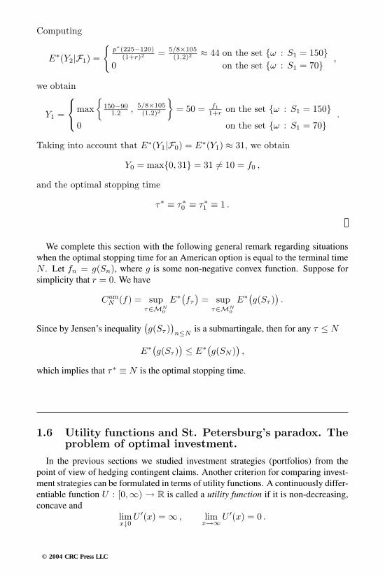
Computing

E∗(Y2|F1) =

p∗(225−120)

(1+r)2 = 5/8×105(1.2)2 ≈ 44 on the set ω : S1 = 150

0 on the set ω : S1 = 70 ,

we obtain

Y1 =

max

150−901.2 , 5/8×105

(1.2)2

= 50 = f1

1+r on the set ω : S1 = 1500 on the set ω : S1 = 70

.

Taking into account that E∗(Y1|F0) = E∗(Y1) ≈ 31, we obtain

Y0 = max0, 31 = 31 = 10 = f0 ,

and the optimal stopping time

τ∗ ≡ τ∗0 ≡ τ∗

1 ≡ 1 .

We complete this section with the following general remark regarding situationswhen the optimal stopping time for an American option is equal to the terminal timeN . Let fn = g(Sn), where g is some non-negative convex function. Suppose forsimplicity that r = 0. We have

CamN (f) = sup

τ∈MN0

E∗(fτ

)= sup

τ∈MN0

E∗(g(Sτ )).

Since by Jensen’s inequality(g(Sτ )

)n≤N

is a submartingale, then for any τ ≤ N

E∗(g(Sτ )) ≤ E∗(g(SN )

),

which implies that τ∗ ≡ N is the optimal stopping time.

1.6 Utility functions and St. Petersburg’s paradox. Theproblem of optimal investment.

In the previous sections we studied investment strategies (portfolios) from thepoint of view of hedging contingent claims. Another criterion for comparing invest-ment strategies can be formulated in terms of utility functions. A continuously differ-entiable function U : [0,∞) → R is called a utility function if it is non-decreasing,concave and

limx↓0

U ′(x) = ∞ , limx→∞U ′(x) = 0 .


An investor’s aim to maximize U(XπN ) can lead to a difficult problem, as Xπ

N is arandom variable. Therefore, it is natural to compare average utilities: we say that astrategy π′ is preferred to strategy π if

E(U(Xπ′

N )) ≥ E

(U(Xπ

N )).

One of the fundamental notions in this area of financial mathematics is the notionof risk aversion. Its mathematical description is given by the Arrow-Pratt function

RA(·) := − U ′′(·)U ′(·)

(in the case when U is twice continuously differentiable). This function characterizesdecreasing of risk aversion if R′

A < 0, and increasing of risk aversion if R′A > 0.

Thus such utility functions allow one to introduce a measure of investment prefer-ences for risk averse participants in a market.

Historically, the theory of optimal investment with the help of utility functionsgrew from the famous Bernoulli’s St. Petersburg’s paradox.

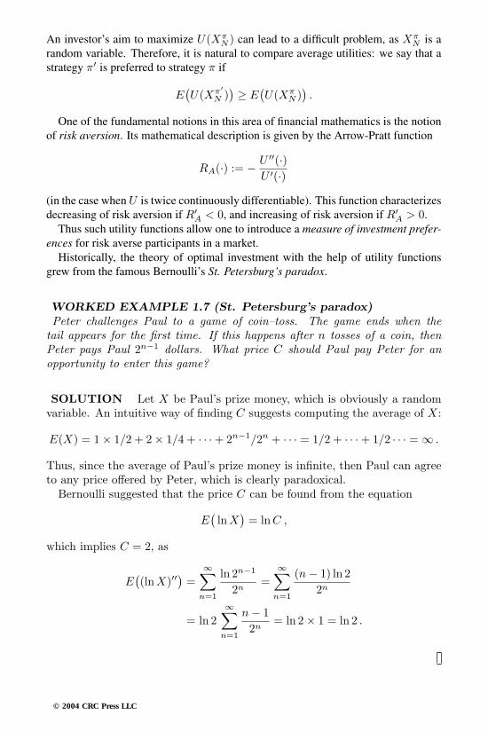
WORKED EXAMPLE 1.7 (St. Petersburg’s paradox)Peter challenges Paul to a game of coin–toss. The game ends when the

tail appears for the first time. If this happens after n tosses of a coin, thenPeter pays Paul 2n−1 dollars. What price C should Paul pay Peter for anopportunity to enter this game?

SOLUTION Let X be Paul’s prize money, which is obviously a randomvariable. An intuitive way of finding C suggests computing the average of X:

E(X) = 1× 1/2 + 2× 1/4 + · · ·+ 2n−1/2n + · · · = 1/2 + · · ·+ 1/2 · · · = ∞ .

Thus, since the average of Paul’s prize money is infinite, then Paul can agreeto any price offered by Peter, which is clearly paradoxical.Bernoulli suggested that the price C can be found from the equation

E(lnX

)= lnC ,

which implies C = 2, as

E((lnX)′′

)=

∞∑n=1

ln 2n−1

2n=

∞∑n=1

(n − 1) ln 22n

= ln 2∞∑

n=1

n − 12n

= ln 2× 1 = ln 2 .


In general, given a utility function U , consider a problem of finding a self-financing strategy π∗ such that

maxπ∈SF

E(U(Xπ

N (x)))

= U(Xπ∗

N (x)). (1.4)

For simplicity, let U(x) = lnx. Then

lnXπN (x) = ln

XπN (x)BN

+ lnBN ,

and therefore, the optimization problem (1.4) reduces to finding the maximum of

E

(ln

XπN (x)BN

)overall π ∈ SF .

Denote Yn(x) := Xπn (x)/Bn the discounted value of a self-financing portfo-

lio π. Recall that (Yn)n≤N is a positive martingale with respect to a risk-neutralprobability P ∗. Thus, we arrive at the problem of finding a positive martingaleY ∗(x) ≡ (Y ∗

n )n≤N with Y ∗0 = x, such that

maxY

E(lnYN (x)

)= E

(lnY ∗

N (x)),

where the maximum is taken over the set of all positive martingales with the initialvalue x.

Let Y ∗N (x) = x/Z∗

N , where Z∗N is the density of the martingale probability P ∗.

All other values of Y ∗(x) are defined as the following conditional expectations withrespect to P ∗:

Y ∗0 = x , Y ∗

n (x) = E∗(

x

Z∗N

∣∣∣∣Fn

), n = 1, . . . , N .

For any other martingale Y we have

E(lnYN (x)

)= E

(ln

x

Z∗N

+[lnYN (x)− ln

x

Z∗N

])≤ E

(ln

x

Z∗N

)+ E

(Z∗

N

x

[YN (x)− x

Z∗N

])= E

(ln

x

Z∗N

)+[E∗(YN (x)

)− E∗(

x

Z∗N

)]/x

= E

(ln

x

Z∗N

)+

x − x

x= E

(ln

x

Z∗N

)= E

(lnY ∗

N (x)).

Thus, Y ∗(x) is an optimal martingale. Recall that, for such a martingale, Y ∗N (x)

necessarily coincides with the discounted value of some self-financing strategy π∗.


To find this optimal portfolio π∗ = (β∗n , γ∗

n)n≤N , we introduce quantities

α∗n := γ∗

n

Sn−1

Xπ∗n−1

,

which represent the proportion of risky capital in the portfolio.Using mathematical induction in N , we obtain

Xπ∗N (x)BN

= xN∏

k=1

(1− α∗

k

1 + r(ρk − r)

),

and on the other hand

Xπ∗N (x)BN

=x

Z∗N

= xN∏

k=1

(1− µ − r

σ2(ρk − r)

)−1

,

where µ = E(ρk

). This gives us the following equation for α∗

k:

N∏k=1

(1− α∗

k

1 + r(ρk − r)

)×(1− µ − r

σ2(ρk − r)

)= 1 .

Let N = 1, then the latter equation reduces to(1− α∗

1

1 + r(ρ1 − r)

)×(1− µ − r

σ2(ρ1 − r)

)= 1 ,

and on the set ω : ρ1(ω) = b we have(1− α∗

1

1 + r(b − r)

)×(1− µ − r

σ2(b − r)

)= 1 ,

which implies that

α∗1 =

(1 + r) (µ − r)(r − a) (b − r)

.

On the set ω : ρ1(ω) = b, the expression for α∗1 is exactly the same. Next,

suppose that α∗1 ≡ α∗

2 ≡ · · · ≡ α∗N−1, then by induction we obtain that α∗

N is alsogiven by this expression.

Thus, the constant proportion of risky capital

α∗ =(1 + r) (µ − r)(r − a) (b − r)

, (1.5)

is a characteristic property of the optimal strategy π∗ that solves the optimizationproblem (1.4) with the logarithmic utility function. Therefore, in this case, man-agement of the risk associated with an investment portfolio reduces to retaining theproportion of risky capital in this portfolio at the constant level (1.5).


Note that management of this type of risk differs from hedging contingent claims.To illustrate this, we revisit Worked Examples 1.3 and 1.4. Recall that in theseexamples we consider a single-period binomial (B,S)-market with the annual rateof interest r = 0.2 and with the profitability of the risky asset

ρ1 =0.5 with probability 0.4−0.3 with probability 0.6 .

The average profitability

m = E(ρ1) = 0.5× 0.4− 0.3× 0.4 = 0.02

is less than r = 0.2, and the optimal proportion of risky capital

α∗ =1.2× (−0.18)0.5× 0.3

≈ −1.5

is negative. This indicates that an investor should prefer depositing money in a bankaccount.

Recall that for the contingent claim in Worked Example 1.3 we have

f1 = (S1 − 100)+ =50 with probability 0.40 with probability 0.6

and its minimal hedging price is 26. For the contingent claim in Worked Example1.4 it is

f1 = maxS0, S1 − S1 =0 with probability 0.430 with probability 0.6

and 9.3, respectively.Now we compute terminal values of optimal investment portfolios with α∗ =

−1.5, and the initial values Xα∗0 = 26:

Xα∗1 = Xα∗

0 +∆Xα∗1 = Xα∗

0 +(r Xα∗

0 + α∗ Xα∗0 (ρ1 − r)

)∣∣∣Xα∗

0 =26

≈33 with probability 0.452 with probability 0.6 =

50 with probability 0.40 with probability 0.6 ,

and Xα∗0 = 9.3:

Xα∗1 = Xα∗

0 +(r Xα∗

0 + α∗ Xα∗0 (ρ1 − r)

)∣∣∣Xα∗

0 =9.3

≈4 with probability 0.414 with probability 0.6 =

0 with probability 0.430 with probability 0.6 .

Thus, the optimal strategy of managing the investment risk differs from both strate-gies of minimal hedging.


REMARK 1.1 In a single-period binomial (B,S)-market, every portfoliocan be associated with the pair (α0, α1) of non-negative real numbers α0, α1 ∈[0, 1] , α0 + α1 = 1, that represent the proportions of the capital invested inassets B and S, respectively. Then the profitability of a portfolio is equal tothe weighted sum of the profitabilities r and ρ1:

ρ(α0, α1) = α0 r + α1 ρ1 .

In this case, the optimal portfolio (α∗0, α

∗1) can be found as a solution to the

following optimization problem

E(ρ(α∗

0, α∗1))= max

(α0,α1)E(ρ(α0, α1)

)under assumption of either

V(ρ(α0, α1)

) ≤ const

orP(

ρ(α0, α1) ≤ const) ≤ c , c ∈ (0, 1) .

Solving this type of optimization problem leads to the introduction of anotion of optimal (effective) portfolio, to the Markovitz theory and to theCapital Asset Pricing model. The concept of Value of Risk also originates fromthis type of problem, and it is widely used in financial practice.

1.7 The term structure of prices, hedging and invest-ment strategies in the Ho-Lee model

Recall that bonds (debentures) are debt securities issued by a government or acompany for accumulating capital. Bonds are issued for a specified period of time[0, N ], where N is called the exercise (redemption) time, and they are characterizedby their face value (redemption cost). Payments up to redemption are called coupons.We consider zero-coupon bonds with face value 1. To satisfy the no-arbitrage condi-tion one has to assume that

0 < B(n,N) < 1 , n < N ,

where B(n,N) is the price at time n of a bond with the exercise time N . Supposethat the evolution of these prices is described by the Ho-Lee model:

B(n + 1, N) =B(n,N)

B(n, n + 1)h(ξn+1;n + 1, N) ,

where (ξn)n≤N is a sequence of independent random variables taking values 0 or1 with probabilities p and 1 − p respectively. The perturbation function h has theproperties: h(· ;N,N) = 1 and h(1;n,N) ≥ h(0;n,N).


As in the case of a binomial (B,S)-market, we can take the probability space(Ω,F , P ) with Ω = 0, 1N∗

, Fn = σ(ξ1, . . . , ξn) and with probability P de-fined by a Bernoulli parameter p ∈ [0, 1]. The family

(B(n,N)

)n≤N∗ is said to be

arbitrage-free if for any n ≤ N∗ the stochastic sequence

(B−1

n B(n,N))n≤N

, where B−1n =

k∏k=0

B(k − 1, k) ,

is a martingale with respect to some probability P ∗.The no-arbitrage condition implies the existence of p = p∗ such that

p∗ h(0;n,N) + (1− p∗)h(0;n,N) = 1 .

Further, there is a δ∗ > 1 such that

h−1(0;n,N) = p∗ + (1− p∗)δN−n∗ ,

h(1;n,N) = δN−n∗

(p∗ + (1− p∗)δN−n

∗)−1

,

andδN−n∗ = h(1;n,N)h−1(0;n,N) .

Now consider the introduced family of bonds(B(n,N)

)n≤N∗ and a bank account

(Bn)n≤N∗ with the rate of interest r ≥ 0. For a perturbation function

h(ξj ; j,N) = δ(N−n)ξj∗ h(0; j,N) ,

we have

B(n,N) =B(0, N)B(0, n)

n∏j=1

h−1(ξj ; j, n)h(ξj ; j,N) .

Further, introducing a new parameter δ = ln δ∗, we can rewrite the perturbationfunction h in the form

h(ξn;n,N) = e(N−n)ξnδ(p∗ + (1− p∗) e(N−n)δ

)−1

.

We obtain the following term structure of bond prices in the Ho-Lee model:

B(n,N) = B(0, N)n∏

i=1

B(i − 1, i)−1

∏ni=1 δ

(N−i)ξi∗∏ni=1

(p∗ + (1− p∗)δ(N−i)

∗)

= B(0, N)Bn

[eδ∑n

i=1(N−i)ξi

/E∗(eδ

∑ni=1(N−i)ξi

)]

=B(0, N)B(0, n)

eδ (N−n)∑n

i=1 ξi

n∏i=1

p∗ + (1− p∗)δ(n−i)∗

p∗ + (1− p∗)δ(N−i)∗

.


Now let us choose a particular bond(B(n,N1)

)n≤N1 from the family(

B(n,N))n≤N≤N∗ . Using it as a risky asset, and a bank account (Bn)n≤N1 as a

non-risky asset, we can form a financial market. A portfolio π is formed by βn unitsof asset Bn and γn(N1) bonds B(n,N1) with the exercise date N1. The values ofthis portfolio are

Xπn = βn Bn + γn(N1)B(n,N1) .

The portfolio π is self-financing if

∆Xπn = βn ∆Bn + γn(N1)∆B(n,N1) .

Thus, this(Bn, B(n,N1)

)n≤N1-market is analogous to the binomial (B,S)-market

with the unique martingale measure P ∗.Let us consider a contingent claim

fN =(B(N,N1)− K

)+, N ≤ N1 ,

which corresponds to the European call option. Its price is uniquely determined by

CN = E∗(B−1

N

(B(N,N1)− K

)+).

Taking into account the term structure of bond prices, we have that B(N,N1) ≥ Kif not less than k0 := k

(N,N1, B(0, N), B(0, N1)

)quantities ξ1, . . . , ξN take value

1, where

k(t, T,B,B′)

= inf

k ≤ t : k ≥ 1

(T − t)δln(

KB

B′

t∏i=1

p∗ + (1− p∗)δ(T−i)

p∗ + (1− p∗)δ(t−i)

).

Denote

B(k0, t, T, p) :=∑ ∏t

i=1 δxi(T−t)∗∏t

i=1

(p∗ + (1− p∗)δ(T−i)

∗) pt−∑ xi (1− p)

∑xi

,

where summation is taken over all vectors (x1, . . . , xt) consisting of 0s and 1s andsuch that

∑xi ≥ k0.

We obtain that

CN = E∗(B−1

N

(B(N,N1)− K

)+)= E∗

((B−1

N B(N,N1)− B−1N K

)+)

= E∗([

B(0, N1)∏N

i=1 δxi(N

1−i)∗∏N

i=1

(p∗ + (1− p∗)δ(N1−i)

∗)

−K B(0, N)∏N

i=1 δxi(N−i)∗∏N

i=1

(p∗ + (1− p∗)δ(N−i)

∗)]+)

= B(0, N1)B(k0, N,N1, p∗)− K B(0, N)B(k0, N,N, p∗) .


Now denoting kn := k(N−n,N1−n,B(n,N), B(n,N1)

), we obtain the structure

of the minimal hedge π∗:

Xπ∗n = Bn E∗

(B−1

N

(B(N,N1)− K

)+∣∣∣Fn

)= B(n,N1)B(kn, N − n,N1 − n, p∗)

−K B(n,N)B(kn, N − n,N − n, p∗) .

On the same market, we now solve the optimization problem (1.4) with the loga-rithmic utility function. Note that the density Z∗

N if probability P ∗ with respect toprobability P has the form

Z∗N = εN

(− p∗ − p

p (1− p)

∑(ξn − (1− p)

)).

Hence, the discounted value of the optimal strategy π∗ = (β∗n, γ∗

n) is

Xπ∗N

BN=

x

Z∗N

= x/

εN

(− p∗ − p

p (1− p)

∑(ξn − (1− p)

)).

Let the proportion of risky capital be

α∗n(N) =

γ∗n(N)B(n − 1, N)

Xπ∗n−1

,

then, since π∗ is self-financing, we obtain

∆Xπ∗

n

Bn= γ∗

n(N)∆B(n,N)

Bn=

Xπ∗n−1 α∗

n(N)B(n − 1, N)

∆B(n,N)

Bn.

Using structure of(B(n,N)

)we write

∆Xπ∗

n

Bn=

Xπ∗n−1 α∗

n(N)Bn−1

[δ(N−n)ξn∗

p∗ + (1− p∗) δN−n∗− 1]

andXπ∗

N

BN= x εN

(∑α∗

n(N)[

δ(N−n)ξn∗

p∗ + (1− p∗) δN−n∗− 1])

,

and therefore arrive at the expression

α∗n(N) =

p∗ − p

p (1− p)δ(N−n)∗ − 1

p∗ + (1− p∗) δN−n∗.


Chapter 2

Advanced Analysis of FinancialRisks

2.1 Fundamental theorems on arbitrage and complete-ness. Pricing and hedging contingent claims in com-plete and incomplete markets.

Let (Ω,FN ,F, P ) be a discrete stochastic basis with filtration F = (Fn)n≤N :

F0 = ∅,Ω ⊆ F1 ⊆ . . . ⊆ FN .

Consider a (B,S)-market with a non-risky asset B defined by a deterministic (orpredictable) sequence of its prices (Bn)Nn=0 , B0 = 1. A risky asset S is defined bya stochastic sequence (of prices) (Sn)Nn=0 adopted to filtration F.

Further, consider the sequence(Sn/Bn

)Nn=0

. We say that a probability P is a mar-

tingale probability if(Sn/Bn

)Nn=0

is a martingale with respect to P . The collectionof all such probabilities is denoted M(

Sn/Bn

).

As in the case of a binomial (B,S)-market, one can consider the notions of aself-financing strategy, a portfolio, etc. Recall that we say that there is an arbitrageopportunity in this market if there exists a self-financing strategy π ∈ SF such thatX π

0 = 0 (a.s.), X πN ≥ 0 (a.s.) and P

(ω : X πN > 0) > 0.

THEOREM 2.1 (First Fundamental Theorem of FinancialMathematics)A (B,S)-market is arbitrage-free if and only if M(

Sn/Bn

) = ∅.

PROOF We prove the ‘if’ part of this statement. For simplicity, supposethat Bn ≡ 1 for all n. Let P ∈ M(

Sn/Bn

), then for any self-financing

strategy π = (β, γ), its discounted value

Xπn = Xπ

0 +n∑

k=1

γk∆Sk

is a martingale with respect to P . Recall that, in the case of binomial markets,this fact is referred to as the martingale characterization of the class SF of


self-financing strategies. Now suppose that π∗ is an arbitrage strategy. By itsdefinition we have E

(Xπ∗

N

)> 0. On the other hand, the martingale property

of(Xπ∗

n

)implies E

(Xπ∗

N

)= E

(Xπ∗

0

)= Xπ∗

0 = 0, which contradicts to theassumption that π∗ is an arbitrage strategy.The proof of the converse is technically far more complex. It can be found,

for example, in [42].

We say that a (B,S)-market is complete if every contingent claim fN can bereplicated by some self-financing strategy, i.e., there exist π ∈ SF and x ≥ 0 suchthat

Xπ0 = x and Xπ

N = fN (a.s.) .

The sequence of discounted prices(Sn/Bn

)Nn=0

is a martingale with respect to any

probability P ∈ M(Sn/Bn

). It turns out that, in the case of a complete market,

it forms a basis for the space of all martingales with respect to P : any martingalecan be written in the form of a discrete stochastic integral with respect to S/B. Thisproperty of a market is called the martingale representation property.

PROPOSITION 2.1A (B,S)-market is complete if and only if it possesses the martingale repre-sentation property.

PROOF For simplicity, suppose that Bn ≡ 1 for all n. Consider a com-plete (B,S)-market. Let (Xn)Nn=0 be an arbitrary martingale and define acontingent claim by fN ≡ XN . The completeness of the market implies thatthere exist π ∈ SF and x ≥ 0 such that

XπN = fN = XN and Xπ

n = x+n∑

k=1

γk ∆Sk (a.s.) .

Since π is a self-financing strategy, the later equality means that (Xn)Nn=0

is a martingale with respect to any probability P ∈ M(Sn/Bn

). Thus we

have two martingales with the same terminal value fN , and therefore for alln = 0, 1, . . . , N

Xπn = E

(fN∣∣Fn

)= Xn ,

which gives us a representation of X in terms of the basis martingale S/B.Conversely, consider a contingent claim fN and a stochastic sequence

(Xn)Nn=0, where Xn = E(fN∣∣Fn

)for any fixed probability P ∈ M(

Sn/Bn

).

Then we can represent this martingale in the form

Xn = X0 +n∑

k=1

φk ∆Sk ,


where (φk)Nk=1 is a predictable sequence. Now let

γ∗n = φn , β∗

n = Xn − γ∗n Sn , n ≤ N .

Note that

β∗n = Xn − γ∗

n Sn = X0 +n−1∑k=1

γ∗k Sk + γ∗

n(Sn − Sn−1)− γ∗nSn

= X0 +n−1∑k=1

γ∗k Sk − γ∗

nSn−1

is completely determined by the information contained in Fn−1, that is,(β∗

n)Nn=0 is a predictable sequence. This implies that π∗ = (β∗

n, γ∗n)

Nn=0 is

a self-financing strategy such that for all n = 0, 1, . . . , N

Xπ∗n = Xn (a.s.) .

In particular, we obtain that Xπ∗N = XN = fN , i.e., an arbitrary contingent

claim fN can be replicated and the market is complete.

The essence of complete markets is characterized in the following result.

THEOREM 2.2 (Second Fundamental Theorem ofFinancial Mathematics)

A (B,S)-market is complete if and only if the set M(Sn/Bn

) = ∅ consistsof a unique element P ∗.

PROOF Consider an arbitrary event A ∈ FN and let fN = IA. Thiscontingent claim can be replicated: there are x > 0 and π ∈ SF such thatXπ

0 = x, XπN (x) = fN , and Xπ

n = x+∑n

k=1 γk ∆Sk for all n = 0, . . . , N .If P1, P2 ∈ M(

Sn/Bn

), then Xπ

n form martingales with respect to boththese probabilities. Therefore

x = Xπ0 = Ei

(Xπ

N

∣∣F0

)= Ei

(Xπ

N

)= Ei

(IA)= Pi

(A), i = 1, 2.

Hence, P1 = P2.Now we sketch the proof of the converse. Let P ∗ be the unique martingale

measure. Using mathematical induction, we will show that Fn = FSn =

σ(S0, . . . , SN ). Suppose Fn−1 = FSn−1. Let A ∈ Fn and define a random

variable

Z = 1 +12

[IA − E

(IA∣∣FS

n

)]> 0 .


Clearly, E∗(Z) = 1 and E∗(Z∣∣FSn

)= 1. Now define a new probability

P ′(C) := E∗(Z IC). We have

E′(∆Sn

∣∣Fn−1

)= E∗(Z∆Sn

∣∣Fn−1

)= E∗(Z∆Sn

∣∣FSn−1

)= E∗

(E∗(Z∆Sn

∣∣Fn−1

)∣∣∣Fn−1

)= E∗

(∆SnE

∗(Z∣∣Fn−1

)∣∣∣Fn−1

)= E∗(∆Sn

∣∣FSn−1

)= 0 ,

which implies that P ′ is a martingale measure. Using the uniqueness of themartingale measure P ∗ we conclude that Z = 1 (a.s.). Hence, IA = E

(IA∣∣FS

n

)and therefore Fn = FS

n .Next consider the following conditional distributions

P ∗(ω : ρn ∈ dx∣∣Fn−1

), where ρn =

∆Sn

Sn−1, n = 1, . . . , N .

It turns out that these distributions have the following structure: there arenon-positive predictable sequence (an)n≤N and non-negative predictable se-quence (bn)n≤N such that

P ∗(ω : ρn = an∣∣Fn−1

)+ P ∗(ω : ρn = bn

∣∣Fn−1

)= 1 , n ≤ N .

The later equality follows from the following result from the general probabil-ity theory: the set of all distributions F (on real line) with the properties∫ ∞

−∞|x| dF (x) < ∞ and

∫ ∞

−∞x dF (x) = 0 ,

consists of a unique distribution F ∗ if and only if there exist a ≤ 0 and b ≥ 0such that F ∗(a) + F ∗(b) = 1.Now let

p∗n := P ∗(ω : ρn = bn∣∣Fn−1

),

1− p∗n := P ∗(ω : ρn = an∣∣Fn−1

).

We have E∗(ρn∣∣Fn−1

)= 0, or equivalently

bn(ω) p∗n + an(ω) (1− p∗n) = 0 .

Thus

p∗n :=−an(ω)

bn(ω)− an(ω),

1− p∗n :=bn(ω)

bn(ω)− an(ω).


Now, if(Xn, F

Sn

)n≤N

is a martingale with respect to P ∗, then there existfunctions fn(x1, . . . , xn) such that

Xn(ω) = fn(ρ1(ω), . . . , ρn(ω)

), n ≤ N .

As in the case of the binomial market, we then arrive to the following mar-tingale representation

Xn = X0 +n∑

k=1

γk ∆Sk ,

where (γk)k≤N is a predictable sequence. Since this is equivalent to the com-pleteness of the market, the proof is completed.

Now we discuss general methodologies of pricing contingent claims in completeand incomplete markets. We start with a complete (B,S)-market that admits aunique martingale measure P ∗. Let fN be a contingent claim. Note that if the prob-ability space (Ω,F , P ) is not finite, then one has to assume that E∗(fN/BN

)< ∞.

Consider the martingale

M∗n := E∗

(fNBN

∣∣∣Fn

), n = 0, 1, . . . , N,

which has the initial and terminal values

M∗0 = E∗(fN/BN

)and M∗

N = fN/BN ,

respectively. By theorem 2.2 M∗ has the following representation

M∗n = M∗

0 +n∑

k=1

γ∗k ∆

Sk

Bk, n = 0, 1, . . . , N,

where (γk)k≤N is a predictable sequence.Define a strategy π∗ = (β∗

n, γ∗n)n≤N with β∗

n = M∗n − γ∗

n Sn/Bn. Then we havethat

β∗n = M∗

0 +n∑

k=1

γ∗k ∆

Sk

Bk− γ∗

n

Sn

Bn

= M∗0 +

n−1∑k=1

γ∗k ∆

Sk

Bk

is a predictable sequence. Hence, we constructed a self-financed strategy π∗ ∈ SFwith values (a.s.) given by

Xπ∗0

B0= M∗

0 ,

∆Xπ∗

n

Bn= γ∗

n

Sn

Bn= ∆M∗

n , n ≤ N ,

Xπ∗n

Bn= M∗

n = E∗(

fNBN

∣∣∣Fn

),


and, in particular, fN = BN a.s.Thus we proved the following result.

THEOREM 2.3 (Pricing Contingent Claims in Complete Markets)

Let fN be a contingent claim in a complete (B,S)-market. Then there existsa self-financing strategy π∗ = (β∗, γ∗) so that it is a minimal hedge with thevalues

Xπ∗n = Bn E∗

(fNBN

∣∣∣Fn

),

and β∗, γ∗ are defined by relations

E∗(

fNBN

∣∣∣Fn

)= E∗

(fNBN

)+

n∑k=1

γ∗k ∆

Sk

Bk,

Xπ∗n = β∗

n Bn + γ∗n Sn .

In particular, the price of fN is

CN = E∗(

fNBN

).

Note that the fact that π∗ is the minimal hedge follows from the followinginequalities:

Xπn

Bn= E∗

(Xπ

N

BN

∣∣∣Fn

)≥ E∗

(fNBN

∣∣∣Fn

)=

Xπ∗n

Bn(a.s.), n = 0, 1, . . . , N ,

for any other π ∈ SF hedging fN .Now we consider incomplete markets. In this case, not every contingent claim can

be replicated by self-financing strategies. Consider a strategy π = (βn, γn)n≤N thatis not necessarily self-financing. We can write

∆Xπn = βn∆Bn + γn∆Sn +Bn−1 ∆βn + Sn−1 ∆γn

= βn∆Bn + γn∆Sn −∆cn ,

where

−∆cn := Bn−1 ∆βn + Sn−1 ∆γn n = 1, . . . , N ; c0 = 0.

Let c = (cn)n≤N be a non-decreasing stochastic sequence (consumption process).A class of strategies (π, c) is then called consumption strategies. Clearly we have

Xπ,cn = Xπ,c

0 +n∑

k=1

(βk ∆Bk + γk ∆Sk

)− cn

= Xπ,c0 +

n∑k=1

(β′k ∆Bk + γk ∆Sk

),


where

β′k := βk − ∆ck

Bk

is not necessarily predictable since the consumption cn is determined by the infor-mation in Fn ⊇ Fn−1.

The discounted value of a consumption strategy (π, c) has the following dynamics:

∆Xπ,c

n

Bn= γn∆

Sn

Bn− ∆cn

Bn−1.

Now let fN be a contingent claim in an incomplete (B,S)-market. If it is possible tofind a consumption strategy (π∗, c∗) that replicates fN , then the value of this strategywill be the natural choice for the price of fN .

Consider the following stochastic sequence

Yn = supP∈M(S/B)

E

(fNBN

∣∣∣Fn

), n = 1, . . . , N, (2.1)

Y0 = supP∈M(S/B)

E

(fNBN

),

YN =fNBN

a.s.

Note that here one has to assume that

supP∈M(S/B)

E

(fNBN

)< ∞ ,

which is obviously satisfied in the case of discrete markets.It turns out that this sequence

(Yn

)n≤N

is a positive supermartingale with respect

to any probability P ∈ M(S/B). Therefore, for a fixed P we can write the Doobdecomposition:

Yn = Y0 + Mn − An , n ≤ N,

where M is a martingale with respect to P and A is a non-decreasing predictablesequence. Clearly, this decomposition depends on the choice of P . The followingoptional decomposition is invariant on the class of martingale measures M(S/B):

Yn = Y0 +M ′n − c′n , n = 0, . . . , N ; M ′

0 = c′0 = 0,

where M ′ is a martingale with respect to any probability from M(S/B) and c′ is anon-decreasing (but not necessarily predictable) stochastic sequence.

Furthermore, M ′ has the following representation

M ′n =

n∑k=1

γ′k ∆

Sk

Bk,


where (γ′k) is a predictable sequence.

Now we define a consumption strategy:

γ∗n = γ′

n , β∗n = Yn − γ∗

n

Sn

Bn, c∗n =

n∑k=1

Bk−1 ∆c′k .

We have

Xπ∗,c∗0 = Y0 = sup

P∈M(S/B)

E

(fNBN

),

∆Xπ∗,c∗

n

Bn= γ∗

n∆Sn

Bn− ∆c∗n

Bn−1= ∆Yn , n ≤ N.

ThusXπ∗,c∗

N

BN= YN =

fNBN

a.s.,

which means that fN is replicated by the consumption strategy (π∗, c∗).We almost proved the following result.

THEOREM 2.4 (Pricing Contingent Claims inIncomplete Markets)Let fN be a contingent claim in an incomplete (B,S)-market. Then there

exists a consumption strategy (π∗, c∗) so that it is a minimal hedge with thevalues

Xπ∗,c∗n = Bn sup

P∈M(S/B)

E

(fNBN

∣∣∣Fn

),

where β∗, γ∗ and c∗ are defined from the optional decomposition of the positivesupermartingale Y (2.1):

Yn = supP∈M(S/B)

E

(fNBN

)+

n∑k=1

γ∗k ∆

Sk

Bk−

n∑k=1

∆c∗kBk−1

,

β∗n =

Xπ∗,c∗n − γ∗

n Sn

Bn.

In particular, the initial (upper) price of fN can be defined as

C∗N = sup

P∈M(S/B)

E

(fNBN

).

PROOF We need to show only that hedge (π∗, c∗) is the minimal hedge.Let (π, c) be an arbitrary consumption strategy hedging fN . Then for anyP ∈ M(S/B) we have

Xπ,cn

Bn≥ E

(Xπ,c

N

BN

∣∣∣Fn

)≥ E

(fNBN

∣∣∣Fn

), n ≤ N,


therefore for all n ≤ N

Xπ,cn

Bn≥ sup

P∈M(S/B)

E

(fNBN

∣∣∣Fn

)=

Xπ∗,c∗n

Bna.s. ,

which proves the claim.

2.2 The structure of options prices in incomplete mar-kets and in markets with constraints. Options-basedinvestment strategies.

Consider an incomplete (B,S)-market. As we noted in the previous section,there may be more than one risk-neutral probability P , and therefore the quantityE(fN/BN

)is not unique.

In this section we discuss arbitrage-free pricing of a contingent claim fN in thecase of incomplete markets.

It is intuitively clear that any number from the interval

[minP

E(fN/BN

), max

PE(fN/BN

)]

can be considered as an arbitrage-free price of a contingent claim fN .

On the other hand, if we denote XπN (x) the terminal value of a strategy with the

initial value x, then we can define quantities

C∗ = minx : Xπ

N (x) ≥ fN for some π ∈ SF,

C∗ = maxx : Xπ

N (x) ≥ fN for some π ∈ SF.

If the set of all risk-neutral measures P consists only of one measure P ∗, then thereexists a hedge π∗ with the initial value CN = E∗(fN/BN

)and with the terminal

value Xπ∗N (CN ) = fN . In this case C∗ = C∗ = C.

In general, C∗ ≤ C∗ and the interval[C∗ , C∗] contains all possible arbitrage-

free prices for fN , i.e., prices that are not risk-free for both parties involved in thecontract. Note that intervals (0, C∗) and (C∗,∞) represent arbitrage prices for thebuyer and for the seller of an option, respectively.


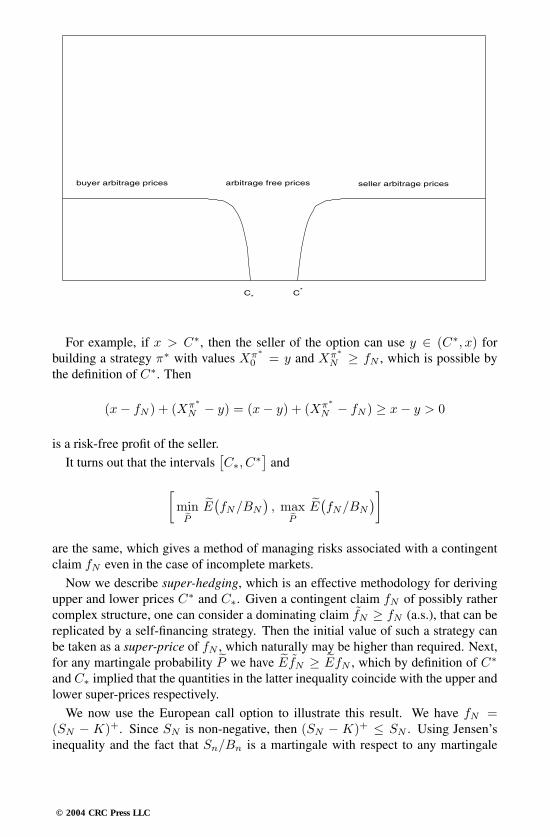
arbitrage free pricesbuyer arbitrage prices seller arbitrage prices

C*

C*

For example, if x > C∗, then the seller of the option can use y ∈ (C∗, x) forbuilding a strategy π∗ with values Xπ∗

0 = y and Xπ∗N ≥ fN , which is possible by

the definition of C∗. Then

(x− fN ) + (Xπ∗N − y) = (x− y) + (Xπ∗

N − fN ) ≥ x− y > 0

is a risk-free profit of the seller.It turns out that the intervals

[C∗, C∗] and

[minP

E(fN/BN

), max

PE(fN/BN

)]are the same, which gives a method of managing risks associated with a contingentclaim fN even in the case of incomplete markets.

Now we describe super-hedging, which is an effective methodology for derivingupper and lower prices C∗ and C∗. Given a contingent claim fN of possibly rathercomplex structure, one can consider a dominating claim fN ≥ fN (a.s.), that can bereplicated by a self-financing strategy. Then the initial value of such a strategy canbe taken as a super-price of fN , which naturally may be higher than required. Next,for any martingale probability P we have EfN ≥ EfN , which by definition of C∗

and C∗ implied that the quantities in the latter inequality coincide with the upper andlower super-prices respectively.

We now use the European call option to illustrate this result. We have fN =(SN − K)+. Since SN is non-negative, then (SN − K)+ ≤ SN . Using Jensen’sinequality and the fact that Sn/Bn is a martingale with respect to any martingale


probability P , we obtain(S0 − K

BN

)+

=(E

(SN

BN

)− K

BN

)+

≤ E

(SN −K

BN

)+

≤ E

(SN

BN

)= E(S0) = S0 .

Thus (S0 − K

BN

)+

≤ C∗ ≤ C∗ ≤ S0 ,

where due to the properties of the market, the first and the last inequalities becomeequalities and give us the lower and the upper prices of the option. The quantityC∗ − C∗, called the spread, is a measure of incompleteness of the market.

Note that complete (B,S)-markets give an idealistic model of real financial mar-kets. Incomplete markets can be regarded as a step toward more realistic models. Afurther step consists of introducing markets with constraints. Now we consider oneof the simplest models of this type. We refer to it as a (B1, B2, S)-market:

∆Bin = ri Bi

n−1 , Bi0 = 1 , i = 1, 2 ,

∆Sn = ρn Sn−1 , S0 ≥ 0 ,−1 < a < r1 ≤ r2 < b ,

where (ρn) is a sequence of independent random variables (representing profitabilityof asset S) that take values b and a with probabilities p and 1− p respectively.

Assets B1 and B2 can be interpreted as saving and credit accounts and S repre-sents shares. It is natural to assume that r1 ≤ r2. If r1 = r2, then B1 = B2 and wearrive to a (B,S)-market.

A strategy (portfolio) π = (πn)n≤N in a (B1, B2, S)-market is defined by threepredictable sequences (β1

n, β2n, γn)n≤N . The values of this strategy are:

Xπn = β1

n B1n + β2

n B2n + γn Sn .

A strategy π is self-financing if

∆Xπn = β1

n∆B1n + β2

n∆B2n + γn∆Sn .

A strategy is admissible if its values are always non-negative. If credit and savingaccounts have different rates of interest, then this creates an arbitrage opportunity.To avoid this, we assume that β1

n ≥ 0 and β2n ≤ 0.

A strategy π will be identified with the corresponding proportion of risky capitalαn = γn Sn−1/X

πn−1. Let (1 − αn)+ and −(1 − αn)− represent an investor’s

deposits in savings and credit accounts, respectively. Then the dynamics of the valuesof such admissible strategy is described by

∆Xπn (x) = Xπ

n−1(x)[(1− αn)+ r1 − (1− αn)− r2 + αn ρn

],

Xπ0 = x > 0 .


Recall that, in a complete arbitrage-free (B,S)-market, contingent claims can bepriced uniquely. In the case of incomplete markets one can find an interval [C∗, C∗]of arbitrage-free prices. The following methodology demonstrates that a similar re-sult holds true in the case of (B1, B2, S)-markets.

Suppose that fN is a contingent claim in a (B1, B2, S)-market. We will introducean auxiliary complete market and find conditions that will guarantee that strategieswith the same proportion of risky capital will have equal values in both markets. Letd ∈ [0, r2 − r1]. Define a (Bd, S)-market:

∆Bdn = rd Bd

n−1 , Bd0 = 1 ,

∆Sn = ρn Sn−1 , S0 ≥ 0 ,

with rate of interest rd = r1 + d.Since the (Bd, S)-market is complete, the price of a contingent claim fN is

uniquely determined by the initial value of the minimal hedge:

CN (f, rd) = Ed

(fNBd

N

),

where expectation is taken with respect to a martingale probability P d.Now let α = (αn)n≤N be the proportion of risky capital, and π(α) and π(α, d)

be the corresponding strategies in the (B1, B2, S)-market and (Bd, S)-market,respectively.

LEMMA 2.1Suppose X

π(α)0 = X

π(α,d)0 . Then X

π(α)n = X

π(α,d)n for all n ≤ N if and only

if(r2 − r1 − d) (1− αn)− + d (1− αn)+ = 0 (2.2)

for all n ≤ N .

PROOF The dynamics of Xπ(α,d)n in the (Bd, S)-market are given by the

following recurrence relation

∆Xπ(α,d)n = βd

n∆Bdn + γn∆Sn = βd

n rd Bdn−1 + γn ρn Sn−1

= rd(βdn Bd

n−1 + γn Sn−1

)+ γn (ρn − rd)Sn−1

= rd Xπ(α,d)n−1 + γn (ρn − rd)Sn−1

= rd Xπ(α,d)n−1 + αn (ρn − rd)Xπ(α,d)

n−1

= Xπ(α,d)n−1

((1− αn) rd + αn ρn

).

Similarly, in the (B1, B2, S)-market we obtain

∆Xπ(α)n = X

π(α)n−1

((1− αn)+ r1 − (1− αn)− r2 + αn ρn

),



This result suggests the following methodology of pricing contingent claims fNin a (B1, B2, S)-market. For any d ∈ [0, r2 − r1] we consider a (Bd, S)-market,where one can use the initial value of the minimal hedge as a price CN (f, rd) forfN . Then quantities

mind

CN (f, rd) and maxd

CN (f, rd)

are obvious natural candidates for lower and upper prices of fN in the (B1, B2, S)-market.

Now we apply this methodology for pricing a European call option, i.e., fN =(SN −K)+. The Cox-Ross-Rubinstein formula gives us prices CN (f, rd) for rd ∈[r1, r2]. Also, it is clear that the function CN (f, ·) is increasing on [r1, r2]. Thus, thelower and upper prices in the (B1, B2, S)-market can be computed by applying theCox-Ross-Rubinstein formula in (Bd, S)-markets with interest rates r1 (in this cased = 0) and r2 (d = r2 − r1), respectively:

CN (ri) = S0 B(k0, N, pi)−K (1 + ri)−N B(k0, N, p∗i ) ,

p∗i =ri − a

b− a, pi =

1 + b

1 + rip∗i , i = 1, 2 .

Note that prices CN (r1) and CN (r2) illustrate the difference of interests of a buyerand a seller in a (B1, B2, S)-market. Price CN (r2) is attractive to a buyer becauseit is the minimal price of the option that guarantees the terminal payment. PriceCN (r1) reflects the intention of a seller to keep the option as an attractive investmentinstrument for a buyer.

WORKED EXAMPLE 2.1Consider a (B1, B2, S)-market with r1 = 0 and r2 = 0.2. Suppose S0 =100($) and

S1 =150 ($) with probability p = 0.470 ($) with probability 1− p = 0.6 .

Find the upper and lower prices for a European call option f1 = (S1 −K)+ ≡max0, S1 −K with strike price K = 100 ($).

SOLUTION From the Cox-Ross-Rubinstein formula we have

C1(0) = S0r1 − a

b− a

1 + b

1 + r1−K (1 + r1)−1 r1 − a

b− a

= 1000.30.8

1.51

− 100 (1)−1 0.30.8

≈ 19 ,

C1(0.2) = 1000.50.8

1.51.2

− 100 (1.2)−1 0.50.8

≈ 26 .


Thus, the spread in such (B 1, B2, S)-market is equal to C1(0.2) − C1(0) =

26− 19 = 7.Now consider the same market with r

1 = 0.1 and r 2 = 0.2. Then we

compute

C1(0.1) = 1000.30.8

1.51.1

− 100 (1.1)−1 0.70.8

≈ 22 ,

and the spread in this case is C1(0.2)− C1(0.1) = 26− 22 = 4.

Note that in this example the condition (2.2) from Lemma 2.1 is satisfied, and theexample illustrates that if the gap r

2 − r 1 between the rates of interest on saving and

credit accounts become smaller, then the spread decreases. Spread can be regardedas a measure of proximity of (B

1, B2, S)-market to an ideal complete market.Next we consider a problem of finding an optimal strategy (a strategy that max-

imizes the logarithmic utility function) in a (B 1, B2, S)-market. By Lemma 2.1 it

is equivalent to solving an optimization problem in a complete (Bd, S)-market. Theoptimal proportion is given by

αn ≡ (1 + rd) (µ− rd)(rd − a) (b− rd)

, d ∈ [0, r2 − r 1].

For the boundary values d = 0 and d = r 2 − r

1 we have

α(i) =(1 + r(i)) (µ− r(i))(r(i) − a) (b− r(i))

, i = 1, 2,

given that α (1) ≤ 1 and α

(2) ≥ 1.In Worked Example 2.1 with r

1 = 0 and r 2 = 0.2 we compute

α(1) =0.02

0.3 · 0.5 ≈ 0.13 ≤ 1, α(2) =−1.02 · 0.180.5 · 0.3 < 1.

Thus, the optimal proportion is 0.13 and the rest of the capital must be invested in asaving account with the rate of interest r1.

Another step in studying more realistic models of a market consists of an intro-duction to transaction costs. Consider the binomial model of a (B,S)-market:

∆Bn = rBn−1 , B0 = 1 ,∆Sn = ρnSn−1 , S0 > 0 ,

where r ≥ 0 is a constant rate of interest with −1 < a < r < b, and 1 ≤ n ≤ N .Now we suppose that any transaction of capital from one asset to another attracts

a fee or a transaction cost (with a fixed parameter λ ∈ [0, 1]): a buyer of asset S paysSn (1 + λ) at time n, and a seller receives Sn (1− λ) accordingly.

Recall that a writer of a European call option is obliged to sell at time N one unitof asset S at a fixed price K. After receiving a premium x, the writer hedges thecorresponding contingent claim by redistributing the capital between assets B and Sin proportion (β, γ).


Suppose that, at terminal time N , both sell and buy prices are equal to SN . Thenthe contingent claim corresponding to this option can be represented here in an ap-propriate two-component form:

f = (f1, f2) =

(−K/BN , 1

)if SN > K

(0, 0) if SN ≤ K ,

where f1 and f2 represent the number of bonds and shares, respectively, necessaryfor making the repayment.

We claim that this model admits a unique ‘fair’ arbitrage-free price CN for suchan option. First, we describe a transition from portfolio π = (β, γ) to portfolioπ′ = (β′, γ′) at some time n ≤ N . Clearly, there are two cases in a situation whenbuying and selling shares attract transaction costs:

1. If γ > γ′, then we have to sell γ − γ′ shares and use the received capitalfor buying the corresponding number of bonds. This leads to the followingcondition

(β′ − β)Bn = (γ − γ′)Sn (1− λ) .

2. If γ < γ′, then we arrive to condition

(β − β′)Bn = (γ′ − γ)Sn (1 + λ) .

Combining these conditions results in

(β′ − β)Bn + (γ′ − γ)Sn = −λ |γ′ − γ|Sn .

Our claim follows from the following theorem (see [10]).

THEOREM 2.5 (Boyle-Vorst)In the framework of a binomial (B,S)-market with transaction costs, for anyEuropean call option there exists a unique replicating strategy. This strategycoincides with the strategy that replicates the same option in a (complete)binomial market without transaction costs, where values b and a of the prof-itability sequence ρ are defined by

1 + b = (1 + b) (1 + λ) and 1 + a = (1 + a) (1− λ) .

PROOF We use the method of reverse induction. First, we introduce thefollowing useful notations for values of Fn-measurable quantities βn+1 andγn+1 on sets ω : ρn = b and ω : ρn = a:

βbn+1(ρ1, . . . , ρn−1) = βn+1(ρ1, . . . , ρn−1, b) ,

βan+1(ρ1, . . . , ρn−1) = βn+1(ρ1, . . . , ρn−1, a) ,

γbn+1(ρ1, . . . , ρn−1) = γn+1(ρ1, . . . , ρn−1, b) ,γan+1(ρ1, . . . , ρn−1) = γn+1(ρ1, . . . , ρn−1, a) .


Then redistribution of capital can be expressed in the form:

(βbn+1 − βn)Bn + (γbn+1 − γn)Sn−1 (1 + b) = −λ |γbn+1 − γn|Sn−1 (1 + b) ,

(2.3)

(βan+1 − βn)Bn + (γan+1 − γn)Sn−1 (1 + a) = −λ |γan+1 − γn|Sn−1 (1 + a) .

Subtracting the second equation from the first, we define function

g(γn) = γn Sn−1 (b− a)− γbn+1 Sn−1 (1 + b) + γan+1 Sn−1 (1 + a)

−βbn+1 Bn + βa

n+1 Bn

−λ |γn − γbn+1|Sn−1 (1 + b) + λ |γn − γan+1|Sn−1 (1 + a) .

Thus, the problem of finding βn and γn given values of βn+1 and γn+1, reducesto the question of solvability of system (2.3), or equivalently, to finding numberif zeros of function g(γn). Note that this function is continuous and linearon intervals (−∞, γa

n+1), (γan+1, γ

bn+1) and (γbn+1,∞) with positive derivative

equal to [(1 + λ) (1 + b)− (1 + λ) (1 + a)

]Sn−1 ,[

(1 + λ) (1 + b)− (1− λ) (1 + a)]Sn−1 ,

and [(1− λ) (1 + b)− (1− λ) (1 + a)

]Sn−1 ,

respectively.Hence g(γn) is a strictly monotone, continuous, piece-wise linear function,

which implies that there is a unique solution to equation g(γn) = 0. Now wehave to show that γn ∈ [γan+1, γ

bn+1], or g(γan+1) ≤ 0 and g(γbn+1) ≥ 0. It is

clear that

g(γan+1) =(γan+1 − γbn+1

)Sn−1 (1 + b) (1 + λ)−Bn βb

n+1 +Bn βan+1 .

Taking into account

γban+2 ≤ γbn+1 ≤ γbbn+2 and γaan+2 ≤ γan+1 ≤ γabn+2 ≤ γban+2 ,

we can rewrite equations (2.3) in the form(βban+2 − βb

n+1

)Bn (1 + r) +

(γban+2 − γbn+1

)Sn−1 (1 + b) (1 + a)

= λ(γbn+1 − γban+2

)Sn−1 (1 + b) (1 + a) ,

and (βban+2 − βa

n+1

)Bn (1 + r) +

(γban+2 − γan+1

)Sn−1 (1 + b) (1 + a)

= λ(γban+2 − γbn+1

)Sn−1 (1 + b) (1 + a) ,


respectively. Subtracting the second equation from the first, we obtain(βan+1 − βb

n+1

)Bn (1 + r) =

(γbn+1 − γan+1

)Sn−1 (1 + a) (1 + b) (1− λ) ,

and hence

g(γan+1) =(γan+1 − γbn+1

)Sn−1 (1 + b)

[(1 + λ)− (1 + a) (1− r)

1 + r

]≤ 0 ,

since γbn+1 ≥ γan+1 and a ≤ r.Similarly, one can prove that g(γbn+1) ≥ 0. To complete the proof, we

need to check the base of induction. At the terminal time, there are twopossible types of portfolios. First: γN+1 = 1, βN+1 = −K, second: γN+1 =βN+1 = 0. Note that in both cases γbN+1 ≥ γaN+1. Suppose γbN+1 = γaN+1,then γN = γbN+1, βN = −K/BN is a unique solution of system (2.3) andγaN+1 ≤ γN ≤ γbN+1.If γbN+1 = 1 and γaN+1 = 0, then the unique solution has the form

γN =SN−1 (1 + b)−K

SN−1 (1 + b)− SN−1 (1 + a)

with γaN+1 = 0 < γN < 1 = γbN+1.The case when γbN+1 = γaN+1 = 0 is trivial:

γN = βN = 0 , γaN+1 ≤ γN ≤ γbN+1 .

Finally, we give examples of typical investment strategies that are based on options(see, for example, [42]).

Straddle is a combination of call and put options on the same stock with the samestrike price K and the same expiry date N . The function V(SN ) := f(SN )−CN is called the gain-loss function. For a buyer we have

V(SN ) = |SN −K| − CN .

Strangle is a combination of call and put options on the same stock with the sameexpiry date N but different strike prices K1 and K2. The gain-loss function inthis case has the form

V(SN ) = |SN −K2| Iω:SN>K2 + |SN −K1| Iω:SN<K1 − CN .

Strap is a combination of one put option and two call options on the same stockwith the same expiry date N but possibly different strike prices K1 and K2. IfK1 = K2, then the gain-loss function has the form

V(SN ) = 2 |SN −K| Iω:SN>K + |SN −K| Iω:SN<K − CN .


Strip is a combination of one call option and two put options on the same stock withthe same expiry date N but possibly different strike prices K1 and K2. Thegain-loss function is given by

V(SN ) = |SN −K2| Iω:SN>K2 + 2 |SN −K1| Iω:SN<K1 − CN .

‘Bull’s’ Spread is a strategy that consists of buying a call option with a strike priceK2 > K1. In this case

V(SN ) = |K2 −K1| Iω:SN≥K2 + |SN −K1| Iω:K1<SN<K2 − CN .

It is usually used in a situation when the stock price is expected to rise.

‘Bear’s’ Spread is a strategy that consists of selling a call option with a strike priceK2 > K1. Then

V(SN ) = −|K2 −K1| Iω:SN≥K2 + |SN −K1| Iω:K1<SN<K2 − CN .

2.3 Hedging contingent claims in mean square

Consider an incomplete (B,S)-market with the time horizon N . As we discussedabove, for (perfect) hedging of contingent claims on such markets, one has to con-sider strategies with consumption.

An alternative approach to hedging of contingent claims was suggested byFoellmer and Sondermann. It is a combination of the ideas of hedging and of in-vestment portfolio with the quadratic utility function.

First we consider a one-step model. Let H be the discounted value of a contingentclaim f1. At time n = 0 the seller of the claim forms a portfolio π0 = (β0, γ0) withvalue

Xπ0 = β0 B0 + γ0 S0,

and the discounted value

V π0 =

Xπ0

B0= β0 + γ0

S0

B0= β0 + γ0 X0,

where X = S/B.At time n = 1 we replace β0 with β1, so that the value of the portfolio becomes

V π1 = β1 + γ0 X1,

where β1 is determined by the replication condition:

V π1 = H or Xπ

1 = f1.


Thus, for finding an ‘optimal’ strategy π one has to determine γ0 = γ. We define thefollowing price sequence Cπ:

Cπ0 = V π

0 , Cπ1 = V π

1 − γ (X1 −X0) = H − γ∆X1 .

This choice has an obvious interpretation: the amount V π1 = H must be paid to the

holder of an option, and γ∆X1 is the gain-loss implied by strategy γ. To determinean optimal γ, one has to solve the following optimization problem: find π such that

V(C π

1

)= inf

πV(Cπ

1

).

Further, if V(∆X1

)> 0, then the variance

V(C π

1

)= V

(H)− 2γ Cov

(H,∆X1

)+ γ2 V

(∆X1

)attains its unique minimum at the point

γ =Cov

(H,∆X1

)V(∆X1

) ,

and therefore

V(C π

1

)= V

(H − γ∆X1

)= V

(H)− Cov2

(H,∆X1

)V(∆X1

)= V

(H)[1− Cov2

(H,∆X1

)].

Another natural optimization problem of finding

infπ

E(Cπ

1 − Cπ0

)2is obviously solved by

Cπ0 = E

(Cπ

1

).

Now we consider an arbitrary time horizon N ≥ 1. It is clear from the one-stepcase that strategies π = (βn, γn)n≤N must be such that γn are predictable (i.e., de-termined by information Fn−1) and βn are adapted (i.e., determined by informationFn).

We have the following discounted values

∆V πn = V π

n − V πn−1 = Xn−1 ∆γn + γn∆Xn +∆βn .

We say that a strategy π is admissible if

V πN = H or Xπ

N = fN .

The price of such a strategy at time n is

Cπn = V π

n −n∑

k=1

γk ∆Xk , n ≤ N.


For simplicity, we assume that the original probability P is a martingale probabilityi.e., P = P ∗. Now we define the following risk sequence

Rπn = E∗

((CπN − Cπ

n

)2∣∣∣Fn

).

Its initial value

Rπ0 = E∗

(H −

N∑k=1

γk ∆Xk − Cπ0

)2

is referred to as risk of strategy π.Note that discounted values of a self-financing strategy π have the form

V πn = V π

0 −n∑

k=1

γk ∆Xk,

which implies that it has a constant price sequence: Cπn = Cπ

0 for all n ≤ N .Now we solve the minimization problem in the class of all admissible strategies.

Suppose that X is a square integrable martingale and E∗(H2)< ∞ (note that in the

case of a discrete probability space (Ω,F , P ∗), these integrability assumptions aretrivially satisfied).

Consider another martingale

V ∗n = E∗(H∣∣Fn

), n ≤ N.

The following decomposition is a key technical tool for solving our problem.

LEMMA 2.2 (Kunita-Watanabe Decomposition)The martingale V ∗ admits the decomposition

V ∗n = V ∗

0 +n∑

k=1

γHk ∆Xk + LHn ,

where(γHn)n≤N

is a predictable sequence and LH is a martingale orthogonalto X:

〈X,LH〉n = 0.

PROOF Define sequence(γHn)n≤N

by

γHn =E∗(H∆Xn

∣∣Fn−1

)E∗((∆Xn)2

∣∣Fn−1

) , n ≤ N, (2.4)

which is clearly predictable. Also let

LHn := V ∗

n − V ∗0 −

n∑k=1

γHk ∆Xk,


which is a martingale being a difference of two martingales.Using Cauchy-Schwartz inequality we obtain

E∗(γHn ∆Xn

)2 = E∗(E∗([

E∗(H∆Xn

∣∣Fn−1

)E∗((∆Xn)2

∣∣Fn−1

) ∆Xn

]2∣∣∣∣Fn−1

))

= E∗((

E∗(H∆Xn

∣∣Fn−1

))2E∗((∆Xn)2

∣∣Fn−1

) )≤ E∗(E∗(H2|Fn−1

))= E∗(H2

)< ∞,

which implies that LH is a square integrable martingale.Now we show that the product

LHn Xn =

(E∗(H|Fn)− E∗(H)−

n∑k=1

γHk ∆Xk

)Xn

forms a martingale. This follows from the definition (2.4) of γHn and theequality

E∗(E∗(H|Fn)Xn

∣∣Fn−1

)− E∗

(γHn ∆Xn Xn

∣∣Fn−1

)= E∗(H|Fn−1)Xn−1 .

Since sequence γH is predictable and LH X is a martingale, then

E∗(LHn

n∑k=1

γHk ∆Xk

∣∣Fn−1

)= E∗(LH

n |Fn−1

) n−1∑k=1

γHk ∆Xk + γHn E∗(LHn ∆Xn|Fn−1

)= LH

n−1

n−1∑k=1

γHk ∆Xk .

Hence, LH is orthogonal to X and(∑n

k=1 γHk ∆Xk

)n≤N

.

Finally, we note that it is not difficult to prove the uniqueness of Kunita-Watanabe decomposition.

Now, since∑n

k=1 γk ∆Xk is a martingale, then to minimize risk Rπ0 we must

have Cπ0 = E∗(H). Furthermore, Rπ

0 does not depend on changes of β, the non-risky component of strategy π. We can rewrite Rπ

0 in the form

Rπ0 = E∗

(H −

N∑k=1

γk ∆Xk − E∗(H))2

= E∗( N∑

k=1

(γHk − γk)∆Xk + LHN

)2

= E∗(LHN

)2 + N∑k=1

E∗((

γHk − γk)2 (∆Xk)2

),


and therefore the required risk-minimizing strategy is uniquely determined by

γn = γHn , n = 1, 2, . . . , N.

Similarly, we obtain the risk sequence

Rπn = E∗

((LHN − LH

n

)2∣∣Fn

).

Thus we obtain the following formulae for the optimal strategy π = (β, γ):

γn = γHn , βn = V ∗n − γn Xn, n ≤ N.

The price of this strategy

C πn = V π

n −n∑

k=1

γk ∆Xk = V ∗n −

n∑k=1

γHk ∆Xk

= E∗(H) +n∑

k=1

γHk ∆Xk + LHn −

n∑k=1

γHk ∆Xk = E∗(H) + LHn

is a martingale. Such strategies π are referred to as self-financing in average.

WORKED EXAMPLE 2.2Consider a one-step (B,S)-market with the rate of interest r = 0.1 and prof-itability

ρ = ρ1 =0.2 with probability 0.7−0.1 with probability 0.3 .

Consider a pure endowment assurance with the claim

f1 = max1 + r, 1 + ρ ,which is paid to the policy holder on survival to time N = 1 (year). Supposethat the probability of death during this year is 0.004, and let B0 = S0 = 1 ($).Find γ and policy’s initial price C0.

SOLUTION Denote C(γ) ≡ Cπ, where π = (β, γ). We need to minimizeV(C1(γ)

)and E

(C1(γ)− C0(γ)

)2. We have

E(max1 + r, 1 + ρ) = 1.1 · 0.3 + 1.2 · 0.7 = 1.17

andV (ρ− r) = V (ρ) = 0.0189 .

If H is the discounted value of the payoff and I1 = IA, where A is the eventof policy holder’s survival for at least one year, then

H = I1max1 + r, 1 + ρ

1 + r.


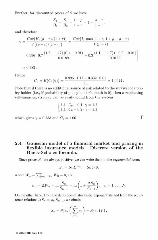
Further, for discounted prices of S we have

S1

B1− S0

B0=

1 + ρ

1 + r− 1 =

ρ− r

1 + r,

and therefore

γ =Cov

(H, (ρ− r)/(1 + r)

)V((ρ− r)/(1 + r)

) =Cov

(I1 max1 + r, 1 + ρ , ρ− r

)V (ρ− r)

= 0.996

[0.7

(1.2− 1.17) (0.1− 0.01)0.0189

+ 0.3(1.1− 1.17) (−0.2− 0.01)

0.0189

]

≈ 0.382 .

HenceC0 = E

(C1(γ)

)=

0.996 · 1.17− 0.332 · 0.011.1

= 1.0624 .

Note that if there is no additional source of risk related to the survival of a pol-icy holder (i.e., if probability of policy holder’s death is 0), then a replicatingself-financing strategy can be easily found from the system

1.1 · C0 + 0.1 · γ = 1.21.1 · C0 − 0.2 · γ = 1.1 ,

which gives γ = 0.333 and C0 = 1.06.

2.4 Gaussian model of a financial market and pricing inflexible insurance models. Discrete version of theBlack-Scholes formula.

Since prices Sn are always positive, we can write them in the exponential form:

Sn = S0 EWn , S0 > 0,

where Wn =∑n

k=1 wk, W0 = 0, and

wn = ∆Wn = lnSn

Sn−1= ln

(1 +

∆Sn

Sn−1

), n = 1, . . . , N.

On the other hand, from the definition of stochastic exponentials and from the recur-rence relations ∆Sn = ρn Sn−1, we obtain

Sn = S0 εn

( n∑k=1

ρk

)= S0 εn

(V),


where we introduced the notation∑n

k=1 ρk = Vn =∑n

k=1 ∆Vk =∑n

k=1 vk withvk = ρk = ∆Vk > −1.

Hence, we obtain the following connection between the two stochastic sequencesW and V :

S0 eWn = Sn = S0 εn

(V)= S0 e

Wn e−Wn

n∏k=1

(1 + ∆Vk

)= S0 e

Wn

n∏k=1

(1 + ∆Vk

)e−∆Wk ,

so

Wn =n∑

k=1

ln(1 + ∆Vk

)and

V =n∑

k=1

(e∆Wk − 1

)= Wn +

n∑k=1

(e∆Wk −∆Wk − 1

).

Now, using Doob decomposition, we can write

Wn = Mn +An, n = 1, . . . , N,

where A0 = M0 = W0 = 0, E(|∆Wn|) < ∞, sequence ∆An = E(∆Wn|Fn−1

)is predictable and ∆Mn = ∆Wn − E

(∆Wn|Fn−1

)forms a martingale.

Thus, prices Sn can be written in the form

Sn = S0 exp Mn +An

on the stochastic basis (Ω,F ,F, P ) where F =(Fn

)n≤N

is a filtration with Fn =σ(S1, . . . , Sn).

Suppose that sequence (wk)k≤N consists of Gaussian random variables withmeans µk and variances σ2

k:

wk ∼ N (µk, σ2k), k = 1, . . . , N.

We can then writewk = µk + σk εk, k = 1, . . . , N,

where εk ∼ N (0, 1) are standard Gaussian random variables. In this case (determin-istic) sequence An and Gaussian martingale Mn have the form

An =n∑

k=1

µk and Mn =n∑

k=1

σk εk ,

and quadratic variation of M is deterministic: 〈M,M〉n =∑n

k=1 σ2k , n ≤ N .


We assume that F = FN = σ(ε1, . . . , εN ). Define a stochastic sequence

Zn = exp

−

n∑k=1

µk

σkεk − 1

2

n∑k=1

(µk

σk

)2

, Z0 = 1, n = 1, . . . , N.

We show that(Zn,Fn

)n≤N

is a martingale with respect to the initial probability P .Indeed, taking into account independence of ε1, . . . , εN , we have

E

(exp

− µk

σkεk − 1

2

(µk

σk

)2)

= 1,

and for all n = 1, . . . , N

E(Zn|Fn−1

)= E

(Zn−1 exp

− µk

σkεk − 1

2

(µk

σk

)2∣∣∣∣∣Fn−1

)

= Zn−1 E

(exp

− µk

σkεk − 1

2

(µk

σk

)2)

= Zn−1 (a.s.).

Now, since ZN > 0 and E(ZN

)= 1, then the following probability

P ∗(A) := E(ZN IA

), A ∈ F

is well-defined. Computing

E∗ (eıλwn)= E

(exp

(ıλσn − µn

σn

)εn + ıλµn − 1

2

(µn

σn

)2)

= E

((ıλσn − µn

σn

)εn − 1

2

(ıλσn − µn

σn

)2)

× exp

12

(ıλσn − µn

σn

)2

+ ıλµn − 12

(µn

σn

)2

= exp− λ2 σ2

n

2

, λ ≥ 0 n = 1, . . . , N,

we conclude that (wk)k≤N is a sequence of Gaussian random variables with respectto P ∗, with mean zero and variance σ2

n. Note that independence of (wk)k≤N follows


from the equality

E∗(exp

ı

N∑k=1

λkwk

)= E∗

(exp

ıN−1∑k=1

λkwk

E∗ (eıλNwN

∣∣FN−1

))

= E∗(exp

ıN−1∑k=1

λkwk

)e−λ2

Nw2N = . . .

= exp− 1

2

N∑k=1

λ2kw

2k

.

As a corollary we obtain the following version of Girsanov theorem.

PROPOSITION 2.2If under probability P random variables

wk ∼ N (µk, σ2k), k = 1, . . . , N

are independent, then they are also independent and normally distributed un-der probability P ∗:

wk ∼ N (0, σ2k), k = 1, . . . , N.

Next we consider the following discrete Gaussian (B,S)-market:

Bn =n∏

k=1

(1 + rk) = exp n∑

k=1

δk

,

Sn = S0 exp n∑

k=1

µk +n∑

k=1

σkεk

, S0 > 0,

where non-negative deterministic sequences (rk) and (δk) represent the rate of inter-est and are such that

1 + rk = eδk , k = 1, . . . , N.

Now our aim is to construct a martingale probability P ∗ for this market. We arelooking for a probability of the form of Essher transform:

P ∗(A) = E(ZN IA

),

where

ZN =N∏

n=1

zn, with zn =exp

an(wn − δn)

E(exp

an(wn − δn)

) ,and (an)n≤N is some deterministic sequence. To find (an)n≤N we use the martin-gale property of

(Sn/Bn

)n≤N

:

E∗(

Sn

Bn

∣∣∣Fn−1

)=

Sn−1

Bn−1, n = 1, . . . , N,


which is equivalent toE∗( expµn + σn εn

)= 1,

where µn = µn − δn , n = 1, . . . , N .Taking into account the expression for Zn, we obtain

E(expan(µn + σn εn) + µn + σn εn

)= E

(expan(µn + σn εn)

)and

E(exp(an + 1)(µn + σn εn)

)= E

(expan(µn + σn εn)

).

Since εn ∼ N (0, 1), then

E(expan σn εn

)= exp(an σn)2/2 ,

which implies

exp(an + 1)µn exp(an + 1)2 σ2n/2 = expanµn expa2

n σ2n/2 ,

µn +σ2n

2= −an σ2

n.

Thus

an = − µn

σ2n

− 12= −µn − δn

σ2n

− 12.

Now using this an we compute

E(expan(wn − δn)

)= E

(exp

−( µn

σ2n

+12

)(µn + σn εn)

)

= exp− µ2

n

σ2n

− µn

2

E

(exp

− σn

( µn

σ2n

+12

)εn

)

= exp− µ2

n

σ2n

− µn

2

exp

σ2n

2

( µn

σ2n

+12

)2

= exp− µ2

n

σ2n

− µn

2

exp

σ2n

2

( µ2n

σ4n

+µn

σ2n

+14

)

= exp− µ2

n

2σ2n

+σ2n

8

,

which gives us

zn = exp−( µn

σn+

σn2

)εn − 1

2

( µn

σn+

σn2

)2

and

ZN = exp−

N∑n=1

[( µn

σn+

σn2

)εn +

12

( µn

σn+

σn2

)2]

.


Now for simplicity we consider a special case of our Gaussian (B,S)-market. Let

Bn = (1 + r)n = eδ n with δ = ln(1 + r), r ≥ 0,

Sn = S0 eWn , S0 > 0.

Here Wn =∑n

k=1 wk , wk = µ + σ εk and εn ∼ N (0, 1) are independent randomvariables on the stochastic basis

(Ω1,F1,F1, P1) ,

where F1 =(F1

n

)n≤N

is a filtration with F10 =

∅,Ω , F1n = σ(ε1, . . . , εn) and

F1 = F1N .

WORKED EXAMPLE 2.3As in Worked Example 1.5 we consider a pure endowment assurance issuedby an insurance company. According to this contract the policy holder is paid

fN = g(SN )

on survival to the time N , where SN is the stock price and g is some functionspecified by the contract. Suppose E

(g2(SN )

)< ∞. Find the ‘fair’ price for

such insurance policy.

SOLUTION Recall that if lx is the number of policy holders of age x,then each policy holder i, i = 1, . . . , lx can be characterized by a positiverandom variable Ti representing the time elapsed between age x and death.Suppose that Ti’s are defined on another probability space (Ω2,F2, P2) withthe filtration F2

n = σ(Ti ≤ k, k ≤ n, i = 1, . . . , lx

).

Denote px(n) = P2

(ω : Ti > n), n = 0, 1, . . . , N , the conditional expec-tation for a policy holder to survive another n years from the age of x (clearly,px(0) = 1).From Bayes’s formula we have

px+n(y) =P2

(ω : Ti > y + x)P2

(ω : Ti > n) =px(y + n)px(n)

,

and hencepx(y + n) = px(n) px+n(y).

Denote

Nn :=lx∑i=1

Iω: Ti≤n

the counter of deaths in the given group of policy holders. Then

E2

(lx −Nn

∣∣F2k

)=(lx −Nk

)px+k(n− k) , k ≤ n ≤ N.


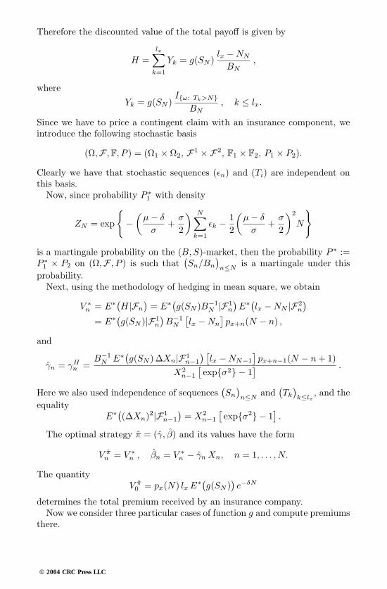
Therefore the discounted value of the total payoff is given by

H =lx∑

k=1

Yk = g(SN )lx −NN

BN,

where

Yk = g(SN )Iω: Tk>N

BN, k ≤ lx.

Since we have to price a contingent claim with an insurance component, weintroduce the following stochastic basis

(Ω,F ,F, P ) = (Ω1 × Ω2, F1 ×F2, F1 × F2, P1 × P2).

Clearly we have that stochastic sequences (εn) and (Ti) are independent onthis basis.Now, since probability P ∗

1 with density

ZN = exp

−(µ− δ

σ+

σ

2

) N∑k=1

εk − 12

(µ− δ

σ+

σ

2

)2

N

is a martingale probability on the (B,S)-market, then the probability P ∗ :=P ∗

1 × P2 on (Ω,F , P ) is such that(Sn/Bn

)n≤N

is a martingale under thisprobability.Next, using the methodology of hedging in mean square, we obtain

V ∗n = E∗(H|Fn

)= E∗(g(SN )B−1

N |F1n

)E∗(lx −NN |F2

n

)= E∗(g(SN )|F1

n

)B−1

N

[lx −Nn

]px+n(N − n) ,

and

γn = γHn =B−1

N E∗(g(SN )∆Xn|F1n−1

) [lx −NN−1

]px+n−1(N − n+ 1)

X2n−1

[expσ2 − 1

] .

Here we also used independence of sequences(Sn

)n≤N

and(Tk

)k≤lx

, and theequality

E∗((∆Xn)2|F1n−1

)= X2

n−1

[expσ2 − 1

].

The optimal strategy π = (γ, β) and its values have the form

V πn = V ∗

n , βn = V ∗n − γn Xn, n = 1, . . . , N.

The quantityV π

0 = px(N) lx E∗(g(SN ))e−δN

determines the total premium received by an insurance company.Now we consider three particular cases of function g and compute premiums

there.


Case 1. Let g(SN ) = SN , then

V ∗n =

[lx −Nn

]Xn px+n(N − n) ,

γn =[lx −Nn−1

]px+n−1(N − n+ 1) ,

βn = Xn

[lx −Nn

]px+n(N − n)− [lx −Nn−1

]px+n−1(N − n+ 1)

= Xn px+n(N − n)

[lx −Nn

]− [lx −Nn−1

]px+n−1(1)

n = 1, . . . , N .

Premium is therefore determined by

V π0 = px(N) lx S0 .

We can compute risk of such strategy:

Rπn =

N∑k=n+1

ek σ2qx+k−1(1) px+k(N − k)

× px+n(N − n)

[lx −Nn

]e−nσ2

X2n ,

Rπ0 =

N∑k=1

ek σ2qx+k−1(1) px+k(N − k)

px(N) lx S2

0 ,

where qy(1) is the probability of death during the year following year y.

The latter formula also implies(Rπ

0

)1/2lx

→ 0 as lx → ∞ ,

which means that if there are enough policy holders, then the company’srisk associated with this contract is infinitesimal.

Case 2. If g(SN ) ≡ K = const, then

V πn = V ∗

n = K e−δN[lx −Nn

]px+n(N − n) ,

γn = 0 , βn = V πn for n = 1, . . . , N ;

V π0 = K e−δN lx px(N) ,

which indicates that in this case one has to invest money in a bankaccount. The risk-sequence here:

Rπn = K2 e−2δN

[lx −Nn

]px+n(N − n) qx+n(N − n), n ≤ N.

In particularRπ

0 = K2 e−2δN lx px(N) qx(N),

and again(Rπ

0

)1/2/lx → 0 as lx → ∞.


Case 3. Let g(SN ) = maxSN ,K. We can write

maxSN ,K = K + (SN −K)+,

and therefore we have to compute

E∗((SN −K)+ ∆Xn

∣∣Fn−1

)and E∗((SN −K)+

∣∣Fn

). (2.5)

For the latter we have

E∗((SN −K)+∣∣Fn

)= E∗((Sn eδ(N−n) ew

∗n+1+···+w∗

N −K)+∣∣Fn

)= E∗

((Sn eδ(N−n) eN

(−σ2

2 (N−n), σ2 (N−n))−K

)+∣∣∣Fn

),

where w∗k = µ− δ+σ εk ∼ N (− σ2

2 , σ2)with respect to probability P ∗.

Note that for ξ ∼ N (0, 1) and constants a, b and K one has

E((

a ebξ−b2/2−K)+) = aΦ

(ln(a/K) + b2/2

b

)−K Φ

(ln(a/K)− b2/2

b

),

where

Φ(x) =1√2π

∫ x

−∞e−y2/2dy

is a standard normal distribution. Hence, we obtain

E∗((SN −K)+∣∣Fn

)= Sn eδ(N−n) Φ

(ln(Sn/K) + (N − n) (δ + σ2/2)

σ√N − n

)

−K Φ(ln(Sn/K) + (N − n) (δ − σ2/2)

σ√N − n

).

Note that for n = 0 we have

E∗((SN −K)+

eδ N

)= S0 Φ

(ln(S0/K) +N (δ + σ2/2)

σ√N

)

−K e−δN Φ(ln(S0/K) +N (δ − σ2/2)

σ√N

),

which is the discrete version of the Black-Scholes formula for a Europeancall option.


Now we compute the first expectation from (2.5):

E∗((SN −K)+Xn

∣∣Fn−1

)= Xn−1 E

∗(ew∗n (SN −K)+

∣∣Fn−1

)= Xn−1 E

∗(E∗(ew

∗n (Sn−1 e

δ(N−n+1) ew∗n+···+w∗

N −K)+∣∣Fn

)∣∣∣∣Fn−1

)

= Xn−1 E∗(ew

∗n

[Sn−1 e

δ(N−n+1) ew∗n

×Φ(ln(Sn−1/K) + w∗

n + (N − n) (δ + σ2/2) + σ2

σ√N − n

)

−K Φ(ln(Sn−1/K) + w∗

n + (N − n) (δ − σ2/2) + σ2

σ√N − n

)]∣∣∣∣∣Fn−1

).

Since for ξ ∼ N (− σ2

2 , σ2)we have

E(eξ Φ(x ξ + y)

)= Φ

(y + σ2 x/2√1 + x2 σ2

),

then

E∗((SN −K)+Xn

∣∣Fn−1

)= Xn−1

[Xn−1 e

δ N expσ2Φ(ln(Sn−1/K) + (N − n+ 1) (δ + σ2/2) + σ2

σ√N − n+ 1

)

−K Φ(ln(Sn−1/K) + (N − n+ 1) (δ − σ2/2) + σ2

σ√N − n+ 1

)].

Thus, we obtain the following formulae for the optimal strategy and itscapital:

V πn = V ∗

n = e−δN[lx −Nn

]px+n(N − n)

×[K + Sn eδ(N−n) Φ

(ln(Sn/K) + (N − n) (δ + σ2/2)

σ√N − n

)

−K Φ(ln(Sn/K) + (N − n) (δ − σ2/2)

σ√N − n

)],


V ∗0 = e−δN lx px(N)

[K + S0 e

δ N Φ(ln(S0/K) +N (δ + σ2/2)

σ√N

)

−K Φ(ln(S0/K) +N (δ − σ2/2)

σ√N

)],

γn =

[lx −NN−1

]px+n−1(N − n+ 1)

Xn−1

[expσ2 − 1

]×Xn−1 e

δ N

[expσ2Φ

(ln(Sn−1/K) + (N − n+ 1) (δ + σ2/2) + σ2

σ√N − n+ 1

)

−Φ(ln(Sn−1/K) + (N − n+ 1) (δ + σ2/2)

σ√N − n+ 1

)]

+K

[Φ(ln(Sn−1/K) + (N − n+ 1) (δ − σ2/2)

σ√N − n+ 1

)

−Φ(ln(Sn−1/K) + (N − n+ 1) (δ − σ2/2) + σ2

σ√N − n+ 1

)],

βn = V ∗n − γn Xn, n = 1, . . . , N.

2.5 The transition from the binomial model of a financialmarket to a continuous model. The Black-Scholesformula and equation.

In previous sections we dealt with discrete markets, where time horizon is de-scribed by integers 0, 1, . . . , N , representing some units of time (e.g., years, monthsetc). Now suppose that we wish to consider a market with time horizon [0, T ] forsome real number T ≥ 0. We can divide this interval into m equal parts, so that wewill have a time scale with the step τ = T/m > 0. Thus, it is natural to consider thefollowing (B,S, τ)-market:

Bτt −Bτ

t−τ = r(τ)Bτt−τ , Bτ

0 > 0, r(τ) > 0,

Sτt − Sτ

t−τ = ρt(τ)Sτt−τ , Sτ

0 > 0,


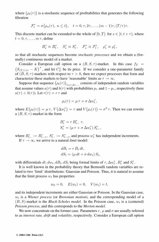
where(ρt(τ)

)is a stochastic sequence of profitabilities that generates the following

filtration

Fτt = σ

(ρn(τ), n ≤ t

), t = 0, τ, 2τ, . . . , (m− 1)τ, (T/τ)τ.

This discrete market can be extended to the whole of [0, T ]: for s ∈ [t, t+ τ), wheret = 0, τ, . . . ,m τ , define

Bτs ≡ Bτ

t , Sτs ≡ Sτ

t , Fτs ≡ Fτ

t , ρτs ≡ ρτt ,

so that all stochastic sequences become stochastic processes and we obtain a (for-mally) continuous model of a market.

Consider a European call option on a (B,S, τ)-market. In this case fT =(S(T/τ)τ − K

)+, and let Cτ

T be its price. If we consider a one-parameter familyof (B,S, τ)-markets with respect to τ > 0, then we expect processes that form andcharacterize these markets to have ‘reasonable’ limits as τ → ∞.

Suppose that sequence(ρt(τ)

)t=τ,2τ,...

consists of independent random variablesthat assume values a(τ) and b(τ) with probabilities pτ and 1−pτ , respectively (herea(τ) < b(τ)). Let r(τ) = r τ and

ρt(τ) = µ τ + σ∆wτt ,

where E(ρt(τ)

)= µ τ, V

(∆wτ

t

)= τ and V

(ρt(τ)

)= σ2 τ . Then we can rewrite

a (B,S, τ)-market in the form

Bτt = r Bτ

t− τ,

Sτt = (µ τ + σ∆wτ

t )Sτt−,

where Bτt− := Bτ

t−τ , Sτt− := Sτ

t−τ , and process wτt has independent increments.

If τ → ∞, we arrive to a natural limit model:

dBt = r Bt dt,

dSt = (µdt+ σ dwt)St,

with differentials dt, dwt, dBt, dSt being formal limits of τ,∆wτt , B

τt and Sτ

t .It is well known in the probability theory that Bernoulli random variables are re-

lated to two ‘limit’ distributions: Gaussian and Poisson. Thus, it is natural to assumethat the limit process wt has properties

w0 = 0, E(wt) = 0, V (wt) = t,

and its independent increments are either Gaussian or Poisson. In the Gaussian case,wt is a Wiener process (or Brownian motion), and the corresponding model of a(B,S)-market is the Black-Scholes model. In the Poisson case, wt is a (centered)Poisson process, and this corresponds to the Merton model.

We now concentrate on the former case. Parameters r, µ and σ are usually referredto as interest rate, drift and volatility, respectively. Consider a European call option


on this continuous market, with the claim fT =(ST −K

)+. We will find its price

using the passage to the limit:

CT = limτ→0

CτT .

Suppose that parameters of the (B,S, τ)-market and of the limit market satisfy therelations

1 + r(τ) = er τ , 1 + b(τ) = eσ√τ , 1 + a(τ) = e−σ

√τ , σ > 0.

Using the Cox-Ross-Rubinstein formula we obtain

CτT = S0 B

(k0(τ), m, pτ

)−K(1 + r(τ)

)−mB(k0(τ), m, p∗τ

),

where

m =T

τ, k0(τ) = 1 +

ln(K/S0

(1 + a(τ)

)m)ln([1 + a(τ)]

/[1 + b(τ)]

) ,and

p∗τ =r(τ)− a(τ)b(τ)− a(τ)

, pτ =1 + b(τ)1 + a(τ)

p∗τ .

By the De Moivre-Laplace limit theorem we have

B(k0(τ), m, p∗τ

) ∼ Φ

(mp∗τ − k0(τ)√mp∗τ (1− p∗τ )

)= Φ

(y∗τ),

B(k0(τ), m, pτ

) ∼ Φ

(mpτ − k0(τ)√mpτ (1− pτ )

)= Φ

(yτ).

Also, for τ → 0

k0(τ) ∼ln(K/S0

)+mσ

√τ

2σ√τ

,(1 + r(τ)

)−m ∼ er T .

Finally, taking into account relations

mp∗τ ∼ T τ(r − σ2/2

)+ T σ

√τ

2σ τ3/2, m pτ−k0(τ) ∼

T τ(r − σ2/2

)+ τ ln(S0/K)

2σ τ3/2,

and √mp∗τ (1− p∗τ ) ∼

√T/4τ ,

we obtain

limτ→0

mp∗τ − k0(τ)√mp∗τ (1− p∗τ )

=ln(S0/K

)+ T

(r − σ2/2

)σ√T

= y∗,

limτ→0

mpτ − k0(τ)√mpτ (1− pτ )

=ln(S0/K

)+ T

(r + σ2/2

)σ√T

= y.


Thus, we arrive to the celebrated Black-Scholes formula:

limτ→0

CτT = CT = S0 Φ(y)−K e−r T Φ(y∗). (2.6)

In general, one can replace interval [0, T ] with [t, T ], where 0 ≤ t ≤ T . In thiscase we consider a contract written at time t with time to expiry T − t. Replacing Tby T − t and S0 by St =: x in formula (2.6), we obtain the corresponding version ofthe Black-Scholes formula:

C(x, t) = St Φ

(ln(St/K

)+ (T − t)

(r + σ2/2

)σ√T − t

)

−K e−r T Φ

(ln(St/K

)+ (T − t)

(r − σ2/2

)σ√T − t

),

which also indicates that price C is a function of time and price of the asset St = x.

PROPOSITION 2.3Suppose that function C(·, ·) is continuously differentiable in t and twice con-tinuously differentiable in x. Then it satisfies the Black-Scholes differentialequation

∂C

∂t+ r x

∂C

∂x+

12σ2 x2 ∂2C

∂x2− r C = 0. (2.7)

PROOF Consider a (B,S, τ)-market with parameters

1 + r(τ) = er τ , 1 + b(τ) = eσ√τ , 1 + a(τ) = e−σ

√τ , σ > 0.

For the martingale probability p∗τ we have

p∗τ =

(erτ − 1

)− (1− e−σ√τ)

eσ√τ − e−σ

√τ

∼ 12

(1 +

r

σ

√τ

)as τ → 0.

Since prices of asset S can take only two possible values on this (B,S, τ)-market, then

erτ C(x, t) = p∗τ C(x eσ√τ , t+ τ) + (1− p∗τ )C(x e−σ

√τ , t+ τ).

Using Taylor’s formula we can write

erτ C(x, t) = (1 + r τ)C(x, t) + o(τ),

C(x eσ√τ , t+ τ)

= C(x, t) +∂C

∂t+ xσ

√τ∂C

∂x+

12σ2 x2 τ

∂2C

∂x2+ o(τ),

C(x e−σ√τ , t+ τ)

= C(x, t) +∂C

∂t− xσ

√τ∂C

∂x+

12σ2 x2 τ

∂2C

∂x2+ o(τ)


for τ → 0, and hence

(1 + r τ)C(x, t) = C(x, t) + τ∂C

∂t+ x r τ

∂C

∂x+

12σ2 x2 τ

∂2C

∂x2+ o(τ),

which implies the claim.

2.6 The Black-Scholes model. ‘Greek’ parameters in riskmanagement, hedging under dividends and budgetconstraints. Optimal investment.

This section is devoted to the rigorous study of the Black-Scholes model of a(B,S)-market with time horizon T < ∞.

Let (Ω,F ,F, P ) be a stochastic basis. Here filtration F = (Ft)t≤T represents acontinuous information flow that is parameterized by a time parameter t ∈ [0, T ]. Itis natural to assume that Ft (being the information up to time t) is a σ-algebra, i.e.,

1. ∅, Ω ∈ Ft;

2. A ∈ Ft ⇒ Ω \A ∈ Ft (closed under taking complements);

3. (Ak)∞k=1 ⊂ Ft ⇒ ∪∞k=1Ak ∈ Ft (closed under taking countable unions);

4. (Ak)∞k=1 ⊂ Ft ⇒ ∩∞k=1Ak ∈ Ft (closed under taking countable intersec-

tions).

The initial information is usually considered to be trivial: F0 = ∅, Ω.On this stochastic basis we consider a Wiener process (Brownian motion) wt, i.e.,

a process with the following properties

(W1) w0 = 0;

(W2) wt − ws and wv − wu are independent for s < t < v < u;

(W3) wt − ws ∼ N (0, t− s).

It is assumed that all ‘randomness’ of the model is generated by this process, andtherefore

Ft = σ(ws, s ≤ t) =: Fwt .

Note that any stochastic process w is a function of two variables: elementary eventω ∈ Ω and time t ≤ T . For a fixed ω, the function w(ω, ·) is called a trajectory.Without loss of generality one can assume that trajectories of a Wiener process arecontinuous in t.


Let us divide interval [0, T ] into n parts: 0 = t0 < t1 < . . . < tn = T , and define

ϕ(t, ω) =n∑

k=1

ϕk−1(ω) I(tk−1,tk](t), (2.8)

where ϕk−1 are square-integrable random variables that are completely determinedby σ-algebras Ftk−1 (in other words, ϕk−1 are Ftk−1 -measurable square-integrablerandom variables).

Now we define a stochastic integral

(ϕ ∗ w)t ≡∫ t

0

ϕ(s, ω) dws :=n∑

k=1

ϕk−1(ω)(wtk∧t − wtk−1∧t

).

It has the following properties

(I1)((αϕ+ β ψ) ∗ w)t = α (ϕ ∗ w)t + β (ψ ∗ w)t;

(I2) E((ϕ ∗ w)T

∣∣Ft

)= (ϕ ∗ w)t;

(I3) E((ϕ ∗ w)t · (ψ ∗ w)t

)= E

( ∫ t

0ϕ(s)ψ(s) ds

),

for any functions ϕ and ψ of type (2.8), and any constants α and β.Next, consider a stochastic function (process)

(ϕt

)t≤T

that is adapted to filtrationF = (Ft)t≤T , i.e. ϕt ≡ ϕ(t, ω) is Ft-measurable for each t ≤ T . If

E(∫ t

0

ϕ2(s, ω) ds < ∞),

then the stochastic integral is well defined for such function ϕ as a mean square limitof integrals of functions of type (2.8), and properties (I1) – (I3) hold true.

Thus, one can consider stochastic processes of the following type

Xt = X0 +∫ t

0

b(s, ω) ds+∫ t

0

a(s, ω) dws , (2.9)

where∫ t

0b(s, ω) ds is a usual Lebesgue-type integral and

∫ t

0a(s, ω) dws is a stochas-

tic integral. Note that equation (2.9) is often formally written in the differential form

dXt = bt dt+ at dwt .

Let F (t, x) be a real-valued function that is continuously differentiable in t andtwice continuously differentiable in x. Then the process Yt := F (t,Xt) is also oftype (2.9), which follows from the celebrated Kolmogorov-Ito formula:

F (t,Xt) = F (0, X0) +∫ t

0

[∂F

∂s(s,Xs) + bs

∂F

∂x(s,Xs) +

12a2s

∂2F

∂x2(s,Xs)

]ds

+∫ t

0

as∂F

∂x(s,Xs) dws . (2.10)


To sketch the proof of this formula, we note that, by Taylor’s formula, incrementsof a smooth function F can be written in the form

∆F (t, x) =∂F

∂x∆x+

∂F

∂t∆t+

12

∂2F

∂x2(∆x)2+

∂2F

∂x∂t∆x∆t+

12

∂2F

∂t2(∆t)2+. . . .

Since ∆wt ∼ N (0,∆t), then increments ∆Xt of process X are equivalent (in dis-tribution) to random variable b∆t+ a ε

√∆t, ε ∼ N (0, 1). Further(

∆Xt

)2 = b2 (∆t)2 + a2 ε2 ∆t+ 2 b a ε (∆t)3/2

andE((∆Xt

)2) = E(a2 ε2 ∆t

)= a2 ∆t .

up to terms of higher order in ∆t.Thus, we obtain the following approximation

∆F (t,Xt) =∂F

∂x

[b∆t+ a ε

√∆t]+

∂F

∂t∆t+

12

∂2F

∂x2a2 ∆t

=(∂F

∂xb+

∂F

∂t+

12

∂2F

∂x2a2

)∆t+

∂F

∂xa ε

√∆t ,

which implies (2.10).We say that a process M = (Mt,Fw

t )t≤T is a martingale on (Ω,F ,F, P ) ifE(|Mt|

)< ∞, and for all s ≤ t

E(Mt|Fs

)= Ms a.s.

If filtration F is generated by a Wiener process w, then any martingale M can bewritten in the form

Mt = M0 +∫ t

0

ϕs dws , (2.11)

for some stochastic function ϕ that is adapted to filtration F and ‘stochastically’integrable with respect to w.

Note that the very construction of a stochastic integral with respect to a Wienerprocess w originates from the martingale property of constructed process. The mar-tingale representation (2.11) is a subtle result saying that stochastic integrals are theonly martingales that exist in this case.

Now we proceed to the Black-Scholes model. Suppose that on a stochastic basis(Ω,F ,F, P ) processes Bt and St are given by

Bt = ert ,

St = S0 e(µ−σ2/2)t+σ wt , S0 > 0 ,

where µ ∈ R and σ > 0.


Applying the Kolmogorov-Ito formula to the process

St = S0 eXt with Xt =

(µ− σ2

2

)t+ σ wt , X0 = 0 ,

we obtain

St = S0 +∫ t

0

[S0 e

Xu

(µ− σ2

2

)+

12eXu σ2

]du+

∫ t

0

σ S0 eXu du

= S0 +∫ t

0

Su µdu+∫ t

0

Su σ dwu = S0 +∫ t

0

Su

(µdu+ σ dwu

).

Thus, the Black-Scholes model can be represented in the following differential form

dBt = r Bt dt ,

dSt = St

(µdt+ σ dwt

), S0 > 0 ,

Parameters r, µ and σ are referred to as rate of interest, profitability and volatilityof the (B,S)-market. In practice, parameters µ and σ are unknown and ought to beestimated, say, from the statistics of prices St. If time intervals between observationsare τ , then we have

St = St−τ eRt , where Rt ∼ N ((µ− σ2/2) τ, σ2 τ),

and therefore µ and σ can be estimated using the fact that process R is normallydistributed with parameters (µ− σ2/2) τ and σ2 τ .

REMARK 2.1 Consider the following linear stochastic equation

dXt = Xt

(µt dt+ σt dwt

) ≡ Xt dYt ,

where X0 is a finite (a.s) random variable,

Yt =∫ t

0

µs ds+∫ t

0

σs dws,

and (in general, random) functions µt and σt satisfy some integrability condi-tions (e.g. µt and σt are bounded). Now we introduce the stochastic exponential

Et(Y ) = expYt − 1

2

∫ t

0

σ2s ds

,

It is not difficult to check that

Xt = X0 Et(Y ), t ≥ 0,

and that the following properties hold true (compare with the discrete casein Section 1.2):


(E1) Et(Y ) > 0 (a.s.);

(E2) 1/Et(Y ) = Et(Y ), where

dYt = −dYt + σ2t dt ;

(E3) If µt ≡ 0 (which implies that Yt is a martingale), then Et(Y ) is a mar-tingale;

(E4) The multiplication rule:

Et(Y 1) Et(Y 2) = Et(Y 1 + Y 2 + [Y 1, Y 2]

),

where

dY it = µi

t dt+ σit dwt , i = 1, 2, and d[Y 1, Y 2]t = σ1

t σ2t dt .

As in binomial case, we can write the Black-Scholes model in terms ofstochastic exponentials:

Bt = B0 Et(r t) ,St = S0 Et(µ t+ σ wt) .

This representation is useful for studying martingale properties of St andSt/Bt.

Now we introduce the standard basic notions related to a (B,S)-market. Ifprocesses β = (βt)t≤T and γ = (γt)t≤T are adapted to filtration F, then π =(πt)t≤T := (βt, γt)t≤T is called a portfolio or strategy on a (B,S)-market. Thecapital (or value) of strategy π is given by

Xπt = βt Bt + γt St .

A contingent claim fT with the repayment date T is defined to be aFT -measurablenon-negative random variable. We say that a strategy π is self-financing if

dXπt = βt dBt + γt dSt .

A self-financing strategy π is called a (perfect) hedge for a contingent claim fT if

Xπt ≥ fT (a.s.).

We say that a strategy π replicates fT if

Xπt = fT .

A hedge π∗ is called the minimal hedge if for any other hedge π and for all t ≤ T

Xπ∗t ≤ Xπ

t .


The price of a contingent claim fT is defined as

CT = Xπ∗0 .

A (B,S)-market is complete if every contingent claim fN can be replicated bysome self-financing strategy. We say that a probability P ∗ is a martingale probabilityif St/Bt is a martingale with respect to P ∗. Similar to the discrete case, P ∗ iscompletely determined by its density Z∗

T :

Z∗T = exp

− µ− r

σwT − 1

2

(µ− r

σ

)2

T

.

The Girsanov Theorem states that in this setting the process

w∗t := wt +

µ− r

σt

is a Wiener process with respect to the new probability P ∗ and the initial filtration F.

Let FY and F ∗Y be distribution functions of a random variable Y with respect to

probabilities P and P ∗, respectively. Then the equality

µT + σ wT = r T + σ wT + (µ− r)T = r T + σ

(wT +

µ− r

σT

)= r T + σ w∗

T

implies that

F ∗µT+σwT

= F ∗rT+σw∗

T= FrT+σwT ,

and therefore

F ∗ST

= F ∗S0 exp

(µ−σ2

2

)T+σ wT

= FS0 exp

(µ−σ2

2

)T+σ wT

.

From the general methodology of pricing contingent claims in complete marketswe have

CT = E∗(

fTBT

)

for any claim fT .


For a European call option with ft =(ST −K

)+, we obtain

CT = E∗(

fTBT

)= e−rT E∗

((ST −K

)+)= e−rT E∗

((S0 exp

(µ− σ2

2)T + σ wT

)+)

= e−rT E

((S0 exp

(r − σ2

2)T + σ wT

)+)

= e−rT E

((S0 exp

(r − σ2

2)T + σ

√T w1

)+)

= e−rT E

((S0 e

rT exp− σ2

2T + σ

√T w1

)+)

= e−rT E

((a ebξ−b2/2 −K

)+)

,

where a = S0 erT , b = σ

√T and ξ ∼ N (0, 1). Here we also used the following

property of a Wiener process:

wT =√T w1 .

Taking into account that

E

((a ebξ−b2/2 −K

)+)= aΦ

(ln(a/K) + 1

2b2

b

)−K Φ

(ln(a/K)− 1

2b2

b

),

we arrive to the Black-Scholes formula:

CT = S0 Φ(ln(a/K) + 1

2b2

b

)−K e−r T Φ

(ln(a/K)− 1

2b2

b

)= S0 Φ

(y+

)−K e−r T Φ(y−),

with

y± =ln(S0/K) + T (r ± σ2/2)

σ√T

.

Thus, we found the ‘fair’ non-arbitrage price of a European call option. As in thecase of binomial markets, we have the following call-put parity relation:

PT = CT − S0 +K e−rT , (2.12)

where PT is the price of a European put option. Relation (2.12) allows us to computePT :

PT = −S0

(1− Φ(y+)

)+K e−rT

(1− Φ(y−)

)= −S0 Φ(−y+) +K e−rT Φ(−y−) .


Note that prices CT and PT are functions of K, σ and S0. Dividing both sides of theidentity

(ST −K)+ − (K − ST )+ = ST −K

by erT and taking expectations with respect to the risk-neutral probability P ∗, weobtain

CT (K,σ, S0)− PT (K,σ, S0) = E∗(ST

)e−rT −K e−rT = S0 −K e−rT .

Finally, using the Black-Scholes formula we write

PT (K,σ, S0) = CT (K,σ, S0)− S0 +K e−rT

= −S0

(1− Φ(y+)

)+K e−rT

(1− Φ(y−)

)= (−S0)Φ

(ln(− S0/(−K)

)+ T (r + (−σ)2/2)

−σ√T

)

−(−K e−r T)Φ

(ln(− S0/(−K)

)+ T (r − σ2/2)

−σ√T

)= CT (−K,−σ,−S0),

which represents the duality of prices of European call and put options.We also can write the price of a European call option at any time t ∈ [0, T ]:

CT (t, St) = St Φ(y+(t)

)−K e−r (T−t) Φ(y−(t)

),

where

y±(t) =ln(St/K) + (T − t)(r ± σ2/2)

σ√T − t

.

This suggests the following structure of the minimal hedge π∗:

γ∗t = Φ

(y+(t)

)=

∂CT

∂S(t, St) ,

β∗t = −K e−r (T ) Φ

(y−(t)

).

Since the option price CT (t, St) is a function of time t, price St, rate if interestr and volatility σ, one can consider the following ‘Greeks’ often used by the riskmanagement practitioners:

Theta:

θ =∂CT

∂t=

St σ ϕ(y+(t)

)2√T − t

−K r e−r (T−t) Φ(y−(t)

),

Delta:

∆ =∂CT

∂S= Φ

(y+(t)

),


Rho:

ρ =∂CT

∂r= K (T − t) e−r (T−t) Φ

(y−(t)

),

Vega:

Υ =∂CT

∂σ= St ϕ

(y+(t)

)√T − t ,

where ϕ(x) = 1√2π

e−x2/2. (Note that since there is no Greek letter ‘vega’, we useupsilon instead.)

Let Yt ≡ Y πt := Xπ

t /Bt ≥ 0 be the discounted value of a portfolio π. The theKolmogorov-Ito formula implies that

dYt = φt dw∗t Y0 = Xπ

0 ,

where φt = σ γt St/Bt and dw∗t = dwt + t (µ − r)/σ is a Wiener process with

respect to probability P ∗.The set

A = A(x, π, fT ) =ω : Xπ

T (x) ≥ fT=ω : Y π

T (x) ≥ fT /BT

is called the perfect hedging set for claim fT and strategy π with the initial wealth x.

The theory of perfect hedging that was discussed above allows one to find a hedgewith the initial wealth X0 = E∗(fT /BT

)and P (A) = 1. However, it is possible

that an investor responsible for claim fT may have initial budget constraints. In par-ticular, an investor’s initial capital may be less than amount X0, which is necessaryfor successful hedging.

Thus, we arrive at the following problem of quantile hedging.

QUESTION 2.1 Among all admissible strategies find a strategy π suchthat

P(A(x, π, fT )

)= max

πP(A(x, π, fT )

)under the budget constraint

x ≤ x0 < E∗(

fTBT

)= X0 ,

where x0 is investor’s initial capital.

The following lemma addresses this problem.

LEMMA 2.3Suppose perfect hedging set A is such that

P (A) = maxπ

P (A) where E∗(

fTBT

IA

)≤ x .


Then a perfect hedge π for the claim fT = fT IA, with the initial wealth x,yields a solution for the problem of quantile hedging. Furthermore, the perfecthedging set A(x, π, fT ) coincides with A.

PROOF

Step 1. Let π be an arbitrary admissible strategy with the initial wealth

x ≤ E∗(

fTBT

)= X0 .

Its discounted value

Yt = x+∫ t

0

φs dw∗s

is a non-negative supermartingale with respect to P ∗. For a perfecthedging set A = A(x, π, fT ) we have

Yt ≥ fTBT

IA , (P − a.s.).

Hence

x = E∗(YT

) ≥ E∗(

fTBT

IA

),

and P (A) ≤ P (A).

Step 2. Let π be a perfect hedge for the claim fT = fT IA, with the initialwealth x satisfying the inequality

E∗(

fTBT

IA

)≤ x ≤ x0 < E∗

(fTBT

)= X0 .

We show that this strategy is optimal for the problem of quantile hedg-ing. Since

x+∫ t

0

φs dw∗s ≥ E∗

(fTBT

IA

)+∫ t

0

φs dw∗s = E∗

(fTBT

IA

∣∣∣Ft

)≥ 0 ,

then π is an admissible strategy. Denote

A′ =ω : x+

∫ T

0

φs dw∗s ≥ fT /BT

the perfect hedging set for π. Since π is a perfect hedge for claim fT ,we obtain

A′ ⊇ ω : fT IA ≥ fT ⊇ A ,

and hence P (A′) ≥ P (A).


Step 3. Now we observe that

A = A , (P − a.s.),

and taking into account that A is a perfect hedging set for π, we concludethat π is optimal strategy for the problem of quantile hedging.

Next, we will use the fundamental Neumann-Pearson Lemma (see [19]) for con-struction of a maximal perfect hedging set.

Suppose that distributions Q∗ and P correspond to hypothesis’ H0 and H1, re-spectively. Let α = EQ∗(φ) be the error of the first kind and β = EP (φ) be thecriterium’s power corresponding to a critical function φ. The Neumann-Pearson cri-terium has the following structure:

φ =

1 , dP/dQ∗ > c

0 , dP/dQ∗ < c,

and it maximizes β given that the error of the first kind does not exceed a set level α.Here c is some constant, and values 0 and 1 in the critical function φ indicate whichof the hypothesis’ H0 or H1 should be preferred.

If we introduce a probability Q∗ by the relation

dQ∗

dP ∗ =fT

BT E∗(fT /BT

) = fT

E∗(fT ) ,then the constraint in Lemma 2.3 can be written in the form

Q∗(A) =∫A

dQ∗

dP ∗ dP ∗ ≤ x

E∗(fT /BT

) = α .

The solution of the corresponding optimization problem is given by

A =ω :

dP

dQ∗ > c

=ω :

dP

dP ∗ > cfT

E∗(fT )

, (2.13)

where

c = inf

a : Q∗

(ω :

dP

dQ∗ > a

)≤ α

, .

The proof of this claim follows from the fundamental Neumann-Pearson Lemma andfrom the equalities

α = EQ∗(φ) = Q∗(A) and β = EP (φ) = P (A) = maxπ

P (A) .

Thus we arrive at the following theorem.


THEOREM 2.6An optimal strategy π for the problem of quantile hedging coincides with the

perfect hedge for the contingent claim fT = fT IA, where the maximal perfecthedging set A is given by (2.13).

Next we consider the problem of quantile hedging for a European call option withfT = (ST −K)+. The initial value of a perfect hedge in this case is

X0 = S0 Φ(d+)−K e−rT Φ(d−) .

Suppose an investor has an initial capital x < X0. By Theorem 2.6 the optimalstrategy for the problem of quantile hedging coincides with the perfect hedge for thecontingent claim fT IA, where

A =ω :

dP

dQ∗ > c

=ω :

dP

dP ∗ > c1 fT e−rT

,

Since density Z∗T has the form

Z∗T = exp

− µ− r

σw∗T +

12

(µ− r

σ

)2

T

, (2.14)

then

A =

ω : exp

µ− r

σw∗T − 1

2

(µ− r

σ

)2

T

> c1 (ST −K)+

=

ω : exp

µ− r

σ2

(lnS0 +

(r − σ2

2

)T + σ w∗

T

)

× exp− µ− r

σ2

(lnS0 +

(r − σ2

2

)T

)− 1

2

(µ− r

σ

)2

T

> c1 (ST −K)+

=

ω : ST

µ− r

σ2exp

− µ− r

σ2

(lnS0 +

µ+ r − σ2

2

)T

> c1 (ST −K)+

.

Now we consider two cases.

Case 1. µ−rσ2 ≤ 1.

Set A can be written in the form

A =ω : ST < d

=ω : w∗

T < b=ω : ST < S0 exp

(r−σ2/2

)T+b σ

for some constants b and d under the constraint

E∗(

fTBT

IA

)= x0 .



ST = S0 exp(

r − σ2

2

)T + σ w∗

T

,

we obtain

P (A) = Φ(b− T (µ− r)/σ√

T

).

Constant b can be found from the equality

x0 = E∗(e−rT fT)IA = e−rT F ∗

T (ST ) ,

where

F ∗T =

1√2π

∫ b/√T

−∞f

(S0 exp

σ√T y +

(r − σ2

2

)T

)e−

y2

2 dy

=1√2π

∫ b/√T

−d0

(S0 exp

σ√T y +

(r − σ2

2

)T

−K

)+

e−y2

2 dy ;

d0 =ln(K/S0

)− T (r − σ2)/2

σ√T

.

Hence

x0 = S0

[Φ(σ

√T − d0)− Φ

(σ√T − b√

T

)]−K e−rT

[Φ(d0)− Φ

(− b√

T

)]= S0

[Φ(d+)− Φ

(σ√T − b√

T

)]−K e−rT

[Φ(d−)− Φ

(− b√

T

)].

Case 2. µ−rσ2 > 1.

Set A can be written in the form

A =ω : w∗

T < b1 ∪ ω : w∗

T > b2

for some constants b1 and b2. Solving the problem of quantile hedging, weobtain

P (A) = Φ(b1 − T (µ− r)/σ√

T

)+Φ

(b2 − T (µ− r)/σ√

T

).

Constants b1 and b2 can be found from the same equality

x0 = E∗(e−rT fT)IA = e−rT F ∗

T (ST ) ,


where now

F ∗T =

1√2π

∫ b1/√T

−∞f

(S0 exp

σ√T y +

r − σ2

2T

)e−

y2

2 dy

+1√2π

∫ ∞

b2/√T

f

(S0 exp

σ√T y +

r − σ2

2T

)e−

y2

2 dy .

Similarly to Case 1,

x0 = S0

[Φ(d+)− Φ

(σ√T − b1√

T

)+Φ

(σ√T − b2√

T

)]

−K e−rT

[Φ(d−)− Φ

(− b1√

T

)+Φ

(− b2√

T

)].

Next, we consider the case when an owner of asset S receives dividends. DenoteSt the process that represents the wealth of the owner of asset S, and let δ St, δ ≥ 0,represent the received dividends. Then the evolution of St is described by followingstochastic equation

d

(St

Bt

)= d

(St

Bt

)+ δ

St

Btdt, δ ≥ 0 .

UsingdSt = St

(µdt+ σ dwt

)and

d

(St

Bt

)=

St

Bt

((µ− r) dt+ σ dwt

),

we obtain

d

(St

Bt

)=

St

Bt

((µ− r + δ) dt+ σ dwt

).

We can notice the analogy of

wt := wt +µ− r + δ

σt with wt = wt +

µ− r

σt

and of

ZT := exp− µ− r + δ

σw∗T +

12

(µ− r + δ

σ

)2

T

,

with Z∗T (see (2.14)).

We now define a new probability PT with density ZT . By Girsanov Theorem,(wt

)t≤T

is a Wiener process with respect to PT . Distribution functions are given by

FµT+σwT= F (r−δ)T+σwT

= F(r−δ)T+σwT


andFST

= FS0 exp (r−δ−σ 2/2)T +σwT .

We compute then the price of a European call option

CT (δ) = E

((ST −K)+

BT

)= e−rT E

((S0 e

(r−σ 2/2)T +σwT −K)+)

= e−rT E

((S0 e

(r−δ−σ 2/2)T +σwT −K)+)

= e−rT E

((S0 e

(r−δ−σ 2/2)T +σ√T w1 −K

)+)

= S0 e−δT Φ

(ln(S0/K) + T (r − δ + σ2/2)

σ√T

)

−K e−rT Φ(ln(S0/K) + T (r − δ − σ2/2)

σ√T

).

In Section 2.2 we studied the binomial model of a market with transaction costs.It was shown in Theorem 2.5 that if the terminal buy and sell prices of stock S areequal, then there exists a unique strategy that replicates the European call option.This strategy is related to a binomial market without transaction costs where valuesof profitability (and therefore, of volatility) are increased.

In the case of the Black-Scholes model, a similar result was proved in [25]. Forsimplicity, suppose that Bt ≡ 1, t ≤ T , and that capital in portfolio π = (β, γ) isredistributed at discrete times ti = i T/N, i ≤ N .

Constraints on redistribution of capital Xπt = βt + γt St of portfolio π can be

written in the form of proportional transaction costs with parameter λ ≥ 0:

∆Xπt = γt∆St − λSt |∆γt| .

Now consider a European call option that will be hedged in the class of strate-gies described above. Denote CBS(ti, Sti), i ≤ N , the capital of a Black-Scholesstrategy. Then an appropriate hedging strategy π must have capital Xπ

t such that

Xπti= CBS(ti, Sti), i ≤ N,

and approximately (up to infinitesimals of high order of ∆t) satisfy equation

∂Xπ(t, St)∂t

+σ2

2S2t

∂2Xπ(t, St)∂s2

= 0 ,

with parameter

σ2 = σ2

(1 + λ

√8

σ π∆t

)> σ2 .


Thus, for pricing European call options in this case one can use the Black-Scholesformula with the increased volatility.

Next, we consider an optimal investment problem in the framework of the Black-Scholes model, where the optimal strategy is defined by the relation

supπ∈SF

E(lnXπ

T

)= E

(lnXπ∗

T

), Xπ

0 = Xπ∗0 = x.

We sketch the solution of this optimal investment problem: find

Y ∗T (x) = sup

YE(lnYT (x)

),

where supremum is taken over the set of all positive martingales with respect to P ∗,starting at x.

Let the optimal martingale be

Y ∗t (x) = E∗

(x

Z∗T

∣∣∣Ft

), t ∈ [0, T ] ,

where

Z∗T = exp

− µ− r

σwT − 1

2

(µ− r

σ

)2

T

is the density of the unique martingale probability P ∗ with respect to P .

As in Section 1.6, it can be shown that

E(lnYT (x)

) ≤ E(lnY ∗

T (x)).

Then using the martingale characterization of self-financing strategies, we obtain

Y ∗t =

Xπ∗t (x)Bt

= X∗t

for some self-financing strategy π∗ =(β∗t , γ

∗t

)t≤T

. Denote

α∗t =

γ∗t St

Xπ∗t

the proportion of risky capital in portfolio π∗. By the Kolmogorov-Ito formula wehave

dX∗t = X∗

t α∗t σ dwt ,

and therefore

X∗T = x exp

σ α∗ wT + α∗ (µ− r)T − 1

2σ2 (α∗)2 T

,

where α∗t ≡ α∗.


On the other hand,

X∗T =

x

Z∗T

= x expµ− r

σwT +

12

(µ− r

σ

)2

T

Comparing these formulae, we deduce the expression for the optimal proportion:

α∗ =µ− r

σ2,

which is often referred to as the Merton’s point.So far we were studying markets with information flow F =

(Ft

)t≤T

defined by

prices of asset S: Ft = σ(S0, . . . , St

). When one wants to take into account the

non-homogeneity of the market, this leads to the assumption that some (but not all!)of the market participants have access to a larger information flow. Mathematicallythis can mean, for example, that the terminal value ST is known at time t < T orthat ST will belong to some interval [S′, S′′] etc. Let ξ be a random variable thatextends market information Ft to Fξ

t = σ(Ft, ξ

). Then Fξ =

(Fξt

)t≤T

is called theinsider information flow. Now we investigate how this additional information can beutilized by a market participant.

For simplicity let r = 0. Using the formula for Merton’s point and the martingaleproperty of the stochastic integral, we obtain that the expected utility is given by

vF(x) = supπ∈SF (F)

E(lnXπ

T (x))

= x+ E

(∫ T

0

αs σ dws +∫ T

0

µαs ds− 12

∫ T

0

α2s σ

2 ds

)= x+ E

(µ2

σ2T − σ2

2µ2

σ4T

)= x+

12

µ2

σ2T

for the information flow F =(Ft

)t≤T

.

When using the insider information flow Fξ =(Fξ

t

)t≤T

, one cannot assume that

the process(wt, Fξ

t

)t≤T

is a Wiener process. Nevertheless, it is natural to assume

that as in Girsanov theorem, there exists a Fξ-adapted process µξ =(µξt

)t≤T

suchthat ∫ T

0

|µξs| ds < ∞ (a.s.) ,

and the process

wt = wt −∫ t

0

µξs ds , t ≤ T ,

is a Wiener process with respect to Fξ.


In this case the additional utility can be expressed in terms of the ‘informationdrift’ µξ. Indeed, for a self-financing strategy π ∈ SF (Fξ) the terminal capital canbe written in the form

XπT (x) = x exp

∫ T

0

αs σ dws − 12

∫ T

0

αs σ2 ds+

∫ T

0

αs (µ+ σ µξs) ds

.


E

(∫ T

0

µ

σµξs ds

)= E

(∫ T

0

µ

σ

(dws − dws

))= 0 ,

we find the expected utility

vFξ(x) = x+12E

(∫ T

0

(µ+ σ µξs)

2

σds

)= x+

12E

(∫ T

0

[µ2

σ2+ (µξ

s)2

]ds

),

given the insider information Fξ. Thus, the additional utility is given by formula

∆ vFξ = vFξ(x)− vF(x) =12E

(∫ T

0

(µξs

)2ds

),

which can be written in more detailed form in many particular cases (see, for exam-ple, [3]).

WORKED EXAMPLE 2.4Find prices of European call and put options on a Black-Scholes market ifr = 0.1, T = 215/365, S0 = 100($), K = 80($), µ = r, σ = 0.1.

SOLUTION By the Black-Scholes formula we have

CT = CT (K,S0, σ) = S0 Φ(y+)−K e−rT Φ(y−)

= 100Φ

(ln(100/80) + 215

365

(0.1 + (0.1)2/2

)0.1√215/365

)

−80 e−0.1 215365 Φ

(ln(100/80) + 215

365

(0.1− (0.1)2/2

)0.1√215/365

)

= 100Φ(3.177)− 80 e−0.1 215365 Φ(3.64) ≈ 24.57 .

The call-put parity can be used now to find the price of a European putoption:

PT = PT (K,S0, σ) = CT − S0 +K e−rT = 24.57− 100 + 80 e−0.1 215365 ≈ 0 .


If we increase the rate of interest to r = 0.2, then

CT ≈ 28.9 and PT ≈ 0 .

Increasing volatility to σ = 0.8 implies higher prices:

CT ≈ 35.55 and PT ≈ 10.97 for r = 0.1 ,

andCT ≈ 38.05 and PT ≈ 9.16 for r = 0.2 .

Finally, for the model with dividends we have

CT (δ, r) = e−δT CT (0, r − δ) and PT (δ, r) = e−δT PT (0, r − δ) .

Let δ = 0.1, then

CT ≈ 18.86 and PT ≈ 0 for r = 0.1 ,

andCT ≈ 23.17 and PT ≈ 0 for r = 0.2 .

For δ = 0.2

CT ≈ 13.5 and PT ≈ 0.04 for r = 0.1 ,

andCT ≈ 17.8 and PT ≈ 0 for r = 0.2 .

2.7 Assets with fixed income

Consider a zero-coupon bond maturing at time T < T ∗, i.e., a claim that pays 1 attime T . Let B(t, T ) be its price at time t ∈ [0, T ]. Naturally we have B(T, T ) = 1and B(t, T ) < 1 for all t ≤ T .

The price B(t, T ) can be written in three equivalent forms:

B(t, T ) = exp− r(t, T ) (T − t)

,

B(t, T ) = exp−∫ T

t

f(t, s) ds

,

B(t, T ) = exp− (T − t) ln

(1 + ρ(T − t, t)

).


Functions r(·, T ) and ρ(T−·, ·) are called yield and yield to maturity, respectively.Function f(t, s), called the forward rate, represents the instantaneous interest rate attime t ≤ s for borrowing at time s.

Under some reasonable assumptions we have the following relations

r(t, T ) = − lnB(t, T )T − t

,

f(t, T ) = − ∂

∂tlnB(t, T ) = r(t, T ) + (T − t)

∂

∂Tr(t, T ) .

Denote rt = f(t, t) the instantaneous short rate at t. This rate of interest can be astochastic process, therefore bonds must be studied as risky assets since their pricesdepend on interest rates.

Let r = (rt)t≥0 be a stochastic process on some stochastic basis (Ω,F ,F, P ).Defining a bank account by

Bt = exp∫ t

0

rs ds

,

we arrive at the notion of a bonds market as a family(Bt, B(t, T )

)t≤T≤T∗

. As

in the case of the studied above (B,S)-market (‘shares’ market) , we can considerdiscounted bond prices:

B(t, T ) =B(t, T )

Bt

and construct a probability P ∗ that is equivalent to the initial probability P andsuch that the process B =

(B(t, T )

)t≥0

is a martingale with respect to P ∗. Ifsuch probability exists, then we say that the bonds market is arbitrage free. We caninterpret the absence of arbitrage as the impossibility of making profit without risk.

Taking into account that B(T, T ) = 1, we obtain

E∗(B−1T

∣∣Ft

)=

B(t, T )Bt

and therefore we have the representation

B(t, T ) = E∗(exp

−∫ t

0

rs ds∣∣∣Ft

),

which allows one to study the structure of prices B(t, T ) by specifying process r =(rt)t≥0.

Here we list some of the frequently used models.

Mertondrt = αdt+ γ dwt , α, γ ∈ R;


Vasicekdrt = (α− β rt) dt+ γ dwt , α, β, γ ∈ R;

Ho-Leedrt = α(t) dt+ γ dwt , γ ∈ R;

Black-Derman-Toydrt = α(t) dt+ γ(t) dwt ,

Hull-Whitedrt = (α(t)− β rt) dt+ γ dwt , β, γ ∈ R;

Another way of specifying process r is given by the Schmidt model: let functionsf and g be continuous, and functions T and F be continuous and strictly increasing.Then define

rt = F(f(t) + g(t)wT (t)

).

All the models listed above can be obtained from the Schmidt model by choosingappropriate functions F, f, g and T .

An equivalent alternative way of describing the structure of bond prices is basedon specifying the evolution of forward rate:

df(t, T ) = σ2 (T − t) dt+ σ dwt ,

orf(t, T ) = f(0, T ) + σ2 t (T − t/2) + σ wt ,

where f(0, T ) is the present forward rate. This implies

drt =(

∂

∂tf(0, t) + σ2 t

)dt+ σ dwt ,

or

rt = f(0, t) +σ2

2t2 + σ wt .

Substituting the expression for f(t, s) into formula

B(t, T ) = exp−∫ T

t

f(t, s) ds

, t ≤ T ,

we obtain∫ T

t

f(t, s) ds =∫ T

t

[f(0, s) + σ2 t (s− t/2)

]ds+ σ (T − t)wt

=∫ T

t

f(0, s) ds+σ2

2t T (T − t) + σ (T − t)wt ,


and hence

B(t, T ) = exp−∫ T

t

f(0, s) ds− σ2

2t T (T − t) + σ (T − t)wt

=B(0, T )B(0, t)

exp− σ2

2t T (T − t) + σ (T − t)wt

.

We can also rewrite it in the form

B(t, T ) =B(0, T )B(0, t)

exp(T − t) f(0, T )− σ2

2t (T − t)2 − (T − t) rt

.

Note that this model is a particular case of the Heath-Jarrow-Morton model, andit is not difficult to check that the initial probability is a martingale probability.

Now we proceed to detailed study of the Vasicek model. According to this modelthe interest rate oscillates around α/β: rt has positive drift if rt < α/β, and negativeif rt > α/β. If α/β = 0, then rt is a stationary (Gaussian) Ornstein-Uhlenbeckprocess.

Applying the Kolmogorov-Ito formula we obtain

rt = e−βt

[r0 +

∫ t

0

α eβt ds+∫ t

0

γ eβt dws

].

Using the Markov property of rt, we can write

B(t, T ) = E

(exp

−∫ T

t

rs ds∣∣∣Ft

)= E

(exp

−∫ T

t

rs ds∣∣∣rt)

= expγ2

2

∫ T

t

(∫ T

s

e−β(u−s) du)2

ds

−α

∫ T

t

∫ u

t

e−β(u−s) ds du− rt

∫ T

t

e−β(u−t) du

≡ exp

a(t, T )− rt b(t, T )

,

where

a(t, T ) :=γ2

2

∫ T

t

(∫ T

s

e−β(u−s) du)2

− α

∫ T

t

∫ u

t

e−β(u−s) ds du

b(t, T ) :=∫ T

t

e−β(u−t) du .

This gives us the general structure of bond prices. Now, in the framework of theVasicek model, we consider a European call option with the exercise date T ′ ≤ T ≤T ∗ and payoff function

f =(B(T ′, T )−K

)+,


where K is the strike price.The price of this option is given by

C(T ′, T ) = B(0, T )Φ(d+)−K B(0, T ′)Φ(d−) ,

where

d± =ln B(0,T )

K B(0,T ′) ± 12 σ2(T ′, T )

( ∫ T

T ′ e−β(u−T ′) du

)2

σ(T ′, T )∫ T

T ′ e−β(u−T ′) du,

σ(T ′, T ) =

(∫ T

T ′

(∫ T

s

γ e−β(u−s) du

)2

ds

)1/2

.

We need to compute

C(T ′, T ) = E

(e−

∫ T ′0 ru du

(B(T ′, T )−K

)+)= E

(Iω:B(T ′,T )>K e−

∫ T ′0 ru du B(T ′, T )

)−K E

(Iω:B(T ′,T )>K e−

∫ T ′0 ru du

)Note that

ω : B(T ′, T ) > K=ω : a(T ′, T )− rT ′ b(T ′, T )) > lnK

=ω : rT ′ ≤ r′

,

where

r′ =lnK − a(T ′, T )

−b(T ′, T ).

Let

ξ = rT ′ η =∫ T

0

ru du ζ =∫ T ′

0

ru du ,

we obtain

C(T ′, T ) = E(Iω: ξ≤r′ e−η

)−K E

(Iω: ξ≤r′ e−ζ

).

To find the final expression for the price, we need the following lemma.

LEMMA 2.4Suppose X and Y are Gaussian random variables. Then

E(Iω:X≤x exp−Y

)= exp

σ2Y

2− µY

Φ(x) ,

E(Iω:X≤x X exp−Y

)= exp

σ2Y

2− µY

[(µX − ρXY )Φ(x)− σX ϕ(x)

],


where

x =x− (µX − ρXY )

σX,

σ2X and σ2

Y are variances of X and Y , ρXY = Cov(X,Y ) and

ϕ(x) =1√2π

e−x2/2 , Φ(x) =∫ x

−∞ϕ(y) dy .

Note that the quantitative characteristics of ξ, η and ζ are given by

µξ = E(rT ′)= e−βT ′

(r0 + α

∫ T ′

0

e−βs ds

),

µη = E

(∫ T

0

ru du

)= r0

∫ T

0

e−βu du+ α

∫ T

0

∫ u

0

e−β(u−s) ds du ,

µζ = E

(∫ T ′

0

ru du

)= r0

∫ T ′

0

e−βu du+ α

∫ T ′

0

∫ u

0

e−β(u−s) ds du ,

σ2ξ = V

(rT ′)= γ2

∫ T ′

0

e−2β(T ′−s) ds ,

σ2η = V

(∫ T

0

ru du

)= γ2

∫ T

0

(∫ T

s

e−β(u−s) du

)2

ds ,

σ2ζ = V

(∫ T ′

0

ru du

)= γ2

∫ T ′

0

(∫ T ′

s

e−β(u−s) du

)2

ds ,

ρξζ = Cov(rT ′ ,

∫ T ′

0

ru du)= γ2

∫ T ′

0

e−β(T ′−s)

∫ T ′

s

e−β(u−s) du ds ,

ρξη = Cov(rT ′ ,

∫ T

0

ru du)= ρξζ + σ2

ξ

∫ T

T ′e−β(u−T ′) du .

Thus

C(T ′, T ) = E(Iω: ξ≤r′ e−η

)−K E

(Iω: ξ≤r′ e−ζ

)= exp

σ2η

2− µη

Φ(r′ − (µξ − ρξη)

σξ

)

−K expσ2

ζ

2− µζ

Φ(r′ − (µξ − ρξζ)

σξ

).

Substituting expressions for µξ, µη, µζ , σ2ξ , σ

2η, σ

2ζ , ρξζ and ρξη into the latter for-

mula, gives us the final expression for the price C(T ′, T ).


Using the observation(K −B(T ′, T )

)+ =(B(T ′, T )−K

)+ −B(T ′, T ) +K ,

we compute the price of a European put option in a(Bt, B(t, T )

)-market:

P (T ′, T ) = K B(0, T ′)Φ(−d−)−B(0, T )Φ(−d+) .

Now we discuss one of the approximation methods for pricing such assets withthe fixed income. Consider a zero-coupon bond with face value 1 and terminal dateT = 1 (say, year). For simplicity, suppose that P ∗ = P (i.e., the initial probabilityis a martingale probability; see for example the Vasicek model). The bond price isgiven by

B(t, T ) = E

(exp

−∫ T

t

rs ds∣∣∣Ft

).

In our case t = 0 and T = 1, hence

B(0, 1) = E

(r0 exp

−∫ 1

0

rs ds∣∣∣F0

)= E

(exp

ln r0 −

∫ 1

0

rs ds)

.

Suppose that the evolution of the interest rate is described by

rt = r0 eat+σwt = eln b+Yt = b eYt ,

wherer0 = b and Yt = a t+ σ wt .

Our further discussion is based on the following methodology, which can be found,for example, in [4]. Let f = f(x), x ∈ R, be a convex function, (ξs)0≤s≤1 be aGaussian process, X :=

∫ 1

0eξs ds and ξ ∼ N (0, 1).

From Jensen’s inequality we have

E(f(X)

)= E

(E(f(X)

)∣∣ξ) ≥ E(f(E(X|ξ))) .

Now choosef(x) = e−bx

and

ξ =∫ 1

0

ws ds

/√V(∫ 1

0

ws ds),

which is clearly a Gaussian random variable. Then

E(ξ) = E

(∫ 1

0

ws ds

/√V(∫ 1

0

ws ds))

=∫ 1

0

E(ws) ds/√

V(∫ 1

0

ws ds)= 0 .


Using the Kolmogorov-Ito formula we write(∫ 1

0

ws ds

)2

= 2∫ 1

0

∫ t

0

ws ds d(∫ t

0

wu du)= 2

∫ 1

0

∫ t

0

ws dswt dt

= 2∫ 1

0

∫ t

0

wt ws ds dt = 2∫ 1

0

∫ t

0

[ws + (wt − ws)

]ws ds dt .

Since increments of w are independent and V (wt) = t, then

E

(∫ 1

0

ws ds

)2

= 2∫ 1

0

∫ t

0

E(w2s

)ds dt = 2

∫ 1

0

∫ t

0

s ds dt

=∫ 1

0

t2 dt =13.

Using the Theorem on normal correlation (see [41]) we can write

E(Yt

∣∣ξ) = a t+ kt ξ ,

where

kt = Cov(Yt, ξ) =√3σ Cov

(wt,

∫ 1

0

ws ds)=

√3σ

∫ 1

0

(1− s) ds

=√3σ(t− t2

2

).

Also

V(Yt

∣∣ ξ) = V(Yt

)− k2t = σ2

(t− 3 t2 + 3 t3 − 3 t4/4

)= νt ,

Cov(Yt Ys

∣∣ ξ) = σ2 mint, s − kt ks = νts .

Now consider

h(ξ) = E

(∫ 1

0

eYs ds∣∣∣ ξ) =

∫ 1

0

eas+ksξ+νs/2 ds .

Computing

LB1 =∫ ∞

−∞h(z)

e−z2/2

√2π

dz ,

gives us the lower estimate for the bond price.To find the upper estimate UB1 we note that there exists a random variable η such

that

E(f(X)

)= E

(f(E(X|ξ)))+ E

([X − E(X|ξ)] f ′(E(X|ξ)))

+12E([

X − E(X|ξ)]2 f ′′(η)).


This implies the estimates

E(f(X)

) ≤ f(E(X|ξ))+ 1

2E([

X − E(X|ξ)]2 f ′′(η))

and

E(f(X)

) ≤ E(f(E(X|ξ)))+ 1

2E([

X − E(X|ξ)]2 supx

f ′′(x)).

Thus

UB1 = LB1 +12c2 E

(V (X|ξ)

),

wherec2 = sup

xf ′′(x) .

One can compute LB1 using standard approximation methods for computing inte-grals. Thus this methodology allows one to approximate bond prices and to computethe corresponding error estimates.

This methodology can also be used for computing prices of options. For example,for a European call option we have

f(x) =(e−bx −K

)+,

and one has to approximate

LB2 =∫ ∞

−∞f(h(z)

) e−z2/2

√2π

dz .

2.8 Real options: pricing long-term investment projects

Long-term investment projects play a significant role in modern economy. Devel-opment of a new enterprise is a typical example of such a project. A company thatplans an investment of this type is often not obliged to realize the project. In thissense such investment activities are similar to a call option on a financial asset. Inboth cases an investor has the right to gain some outcomes of a project in return forinvested capital (e.g., buy shares at a strike price). Such investment programs in ‘realeconomy’ are referred to as real options (see, for example, [13]).

This similarity suggests that methods of managing risk related to contingent claimsmay be helpful in managing risk related to long-term investment projects.

Let us consider a project with a fixed implementation date T . As before, we willuse the notion of a basic asset, which represents the expected result of the project.Let St be its price, then it is natural to expect that the price of the project is givenby some function F (ST ). Clearly, this quantity must reflect the discounted yieldgenerated by the basic asset S.


Studying the profitability of the investment project is essential for making a deci-sion about its realization. If I is a fixed capital of a proposed investment, then it mustbe compared with some level of profitability R, which depends on F (ST ):

If I ≤ R , then the project is accepted for realization;If I > R , then the project is rejected.

How to find sensible values of R? If evolution of the basic asset is deterministic,then its price can be written in the form

Sdett = expst ,

where st is a deterministic function of t ∈ [0, T ]. If r is the rate of interest, then thelevel of profitability can be defined as

R = Rdet0 = e−rT F

(SdetT

).

If evolution of price of S is not deterministic, then we model it in terms of Sdett

perturbed by a Gaussian white noise with mean zero and variance σ2. Then theexpectation of price Snoise

t will coincide with price’s deterministic component:

E(Snoiset

)= Sdet

t = expst , S0 = 1 .

The evolution of prices is given by

Snoiset = Sdet

t expσ wt − σ2

2t= exp

st + σ wt − σ2

2t,

where w is a Wiener process.

Sdett

Tt

Snoiset

Tt


Then it is natural to define

Rnoiseσ = E

(e−rT F

(SdetT

))= e−rT

∫ ∞

−∞F(SdetT exp

√T σ x− σ2

2T) e−x2/2

√2π

dx

=e−rT

√2π

∫ ∞

−∞F(exp

sT +

√T σ x− σ2

2T)

e−x2/2 dx

→ Rdet0 as σ → 0 .

Alternatively, one can define R as the expectation of F(ST

)with respect to a

risk-neutral probability P ∗ (see [26]) whose density with respect to P is

Z∗T = exp

r

σwT − 1

2

( r

σ

)2

T.

By Girsanov theorem, the process

w∗t = wt − r

σt

is a Wiener process with respect to P ∗. Thus, we obtain another value of R:

R = R∗ = E∗(e−rT F

(ST

))= E∗

(e−rT F

(exp

sT + σ wT − σ2

2T))

= e−rT E∗(F(esT +rT exp

σ wT − r T − σ2

2T))


σ(wT − r

σT)− σ2

2T))


σ w∗

T − σ2

2T))

=e−rT

√2π

∫ ∞

−∞F(exp

sT + r T +

√T σ x− σ2

2T)

e−x2/2 dx .

In some types of long-term investment projects it is natural to assume that the totalvalue of an investment and the implementation date are not known in advance. Forexample, investments in scientific research or in the production of energy are projectsof this type.

Suppose we know the final cost of the basic asset, and let Xt, t ≥ 0 be the amountof capital necessary for completion of the project. As a particular example, considerthe Pindyck model, where random process X satisfies the following stochastic dif-ferential equation

dXt = −αt dt+ β√

αt Xt dwt , X0 = x ,


where β > 0 and αt is the intensity of the investment flow.Since investment potential is often limited, and it is not possible to reverse the

investment flow, then it is natural to assume that α = (αt) is a bounded randomvariable. For simplicity, say αt ∈ [0, 1]. Process α plays the role of control in theprocess of spending the investment capital Xt = Xα

t . Choosing α from the set of alladmissible processes

ג =α : αt ∈ [0, 1]

implies defining a natural implementation time

τ = τα = inft : Xt = Xα

t = 0

for a project.If V is the final cost of the project and r is the rate of interest, then the quantity

V e−rτ −∫ τ

0

αt e−rt dt

represents the profit gained by choosing the investment strategy α. The average profitis given by

vα(x) = Ex

(V e−rτ −

∫ τ

0

αt e−rt dt),

where notation Ex for mathematical expectation indicates that the initial investmentx was necessary for completion of this project.

Since all control strategies belong to the class ,ג it is natural to define the optimalstrategy α∗ from

v(x) ≡ supα∈ג

vα(x) = vα∗(x) . (2.15)

Problems of this type are usually solved by the method of dynamic programming,where one of the main tools is the Bellman principle. Here we briefly sketch thismethod (for more details see [23]).

Suppose that the controlled process Xt = Xαt satisfies the stochastic differential

equationdXt ≡ dXα

t = bα(Xαt ) dt+ σα(Xα

t ) dwt , X0 = x ,

where bα and σα are some reasonable functions (for example, satisfying Lipschitzcondition), and α is a control process that is adapted to a σ-algebra generated by Xt.

For estimating the quality of control α we introduce a function fα(x), α ∈[0, 1], x ∈ R, which is interpreted as the intensity of the profit flow. Then thetotal profit on interval [0, t] is equal to∫ t

0

fα(Xαs ) ds .

Denoting

vα(x) = Ex

(∫ ∞

0

fα(Xs) ds)


its expectation on [0,∞), we will find the optimal control α∗ from condition (2.15):

v(x) ≡ supα∈ג

vα(x) = vα∗(x) .

We use the Bellman principle:

v(x) = supα∈ג

Ex

(∫ t

0

fα(Xαs ) ds+ v(Xα

t ))

, t > 0 , (2.16)

for determining the price v(x). We briefly explain the motivation for using it. Let uswrite the total profit of using strategy α in the form∫ ∞

0

fα(Xs) ds =∫ t

0

fα(Xs) ds+∫ ∞

t

fα(Xs) ds .

If this strategy was used only up to time t, then the first term in the right-handside represents the profit on interval [0, t]. Suppose the controlled process has valuey = Xt at time t. If we wish to alter the control process after time t with the aimof maximizing the profit over the whole of [0,∞), then we have to maximize theexpectation

Ey

(∫ ∞

t

fα(Xs) ds)

,

where α also denotes the continuation of the control process to [t,∞). Changingvariable s = t+u, u ≥ 0, and using independence and stationarity of increments ofthe Wiener process, we obtain

EXt

(∫ ∞

t

fα(Xs) ds)= vα(Xt) ≤ v(Xt) ,

Thus, a strategy that is optimal after time t, gives the average profit such that

Ex

(∫ t

0


t ))≥ vα(x) .

One can choose αs, s ≥ t, so that the corresponding profit is close enough to theaverage profit. Hence, taking supremum of both sides of the latter inequality yieldsthe Bellman principle (2.16). If we a’priori assume that the Bellman function issmooth enough, then the Bellman principle can be written in the following differen-tial form

v(Xαt ) = v(x) +

∫ t

0

[∂v

∂xbα(Xα

s ) +12

∂2v

∂x2σ2α(X

αs )]ds

+∫ t

0

∂v

∂xσα(Xα

s ) dws ,


where Kolmogorov-Ito formula was used. Since the last term in the right-hand sideis a martingale, then we obtain

v(x) = supα∈ג

Ex

(∫ t

0


t ))

= supα∈ג

Ex

(∫ t

0

[∂v

∂xbα(Xα

s ) +12

∂2v

∂x2σ2α(X

αs ) + fα(Xα

s )]ds+ v(x)

).

Hencesupα∈ג

[Lα v(x) + fα(x)

]= 0 ,

where

Lα v =∂v

∂xbα +

12

∂2v

∂x2σ2α .

The latter relation is usually referred to as Bellman differential equation.Note that the considered investment problem controls process Xα

t only up to thetime

τ = ταD

of its exit from region D. Thus this problem can be written in the following generalform

v(x) = supα∈ג

Ex

(∫ ταD

0

fα(Xαs ) e

−rs ds+ g(Xατα

D) e−rτα

D

),

where g = g(x) is some function defined on the boundary ∂D of set D. In this casewe again arrive at a Bellman differential equation

supα∈ג

[12

∂2v

∂x2σ2α(x) +

∂v

∂xbα(x)− r v(x) + fα(x)

]= 0 ,

which is satisfied by Bellman function v for sufficiently wide class of coefficientsbα(x) and σα(x), α ∈ [0, 1], x ∈ R.

Consider again an investment problem in Pindyck model (see [36]). We note that

fα(x) = α, g(x) = V, D = x : x > 0 .

Then Bellman differential equation has the form

r v(x) = supα∈ג

[− α− α

∂v

∂x+

β2

2αx

∂2v

∂x2

],

or, taking into account linearity in α

r v(x) =−1− ∂v

∂x + β2

2 x ∂2v∂x2 if −1− ∂v

∂x + β2

2 x ∂2v∂x2 > 0

0 otherwise .


It is clear that the investment strategy

α∗t =

1 if Xt < x∗

0 if Xt ≥ x∗ ,

where x∗ is a solution of v(x∗) = 0, is a candidate for being optimal.Consider differential equation

r v(x) = −1− ∂v

∂x+

β2

2x∂2v

∂x2.

Its general solution has the form

v(x) = c1 xν/2 Jν

(2−

√b x)+ c2 x

ν/2 H1ν

(2√−b x

)+ (1− ν) b ,

where ν = 1 + 2/β2, b = 2 r/β2,

Jν(x) =∞∑k=0

(−1)k (x/2)ν+2k

k! Γ(ν + k + 1)

is Bessel function of the first kind, Γ is gamma-function and H(1)ν is Hankel function

of the first kind.This solution can be also written in terms of modified Bessel functions:

Iν(x) =∞∑k=0

(x/2)ν+2k

k! Γ(ν + k + 1),

Kν(x) =π

2I−ν(x)− Iν(x)

sin(πν), ν /∈ Z ,

Kn(x) = (−1)n+1 In(x) ln(x/2) +12

n−1∑k=0

(−1)k (n− k − 1)!k!

(x/2)2k−n

+(−1)n2

n∑k=0

(x/2)2k+n

k! (n+ k)!

[Ψ(n+ k + 1) + Ψ(k + 1)

], n ∈ Z ,

where Ψ is the logarithmic derivative of Γ. We have

v(x) = c1 (−1)ν/2 xν/2 Iν(2√b x)+c2

2π(−1)(ν+1)/2 xν/2 Kν

(2√b x)+(1−ν)/b .

Since

xν/2 Iν(2√b x)= xν/2

∞∑k=0

(b x)ν/2+k

k! Γ(ν + k + 1)→ 0 as x → 0 ,

then the initial condition v(0) = V allows to compute

c2 =

sin(πν) Γ(1− ν) bν/2 (−1)−(ν+1)/2(V + 1

r

)if ν /∈ Z

π(n−1)! b

ν/2 (−1)−(ν+1)/2(V + 1

r

)if ν ∈ Z .


Note that we are solving a problem with an unknown boundary. In the theory of dif-ferential equations, such problems are referred to as Stefan problems. The method-ology of dealing with such problems involves the ideas of continuity and smoothgluing on the boundary x = x∗:

v(x∗) = 0 and v′(x∗) = 0 .

This implies

c1 = (−1)−ν/2 Kν−1

(2√b x∗)

Iν−1

(2√b x∗) ,

v(x) =Kν−1

(2√b x∗)

Iν−1

(2√b x∗) xν/2 Iν

(2√b x)+ cKν

(2√b x)+ (1− ν)/b ,

where c = 2π c2.

Now we have to check that the constructed function v and control α∗ indeed solvethe initial investment problem. The ‘verification conditions’ in this case are

1) vα(x) ≤ v(x) for any α and x;

2) vα∗(x) = v(x) for x ≥ 0.

Here is the sketch of this verification. From the properties of Bessel functions wehave that the solution to

β2

2x∂2v

∂x2− ∂v

∂x− r v − 1 = 0

is a smooth function. Also

β2

2αx

∂2v

∂x2− α

∂v

∂x− r v − α ≤ 0

for α ∈ [0, 1]. Further, using the Kolmogorov-Ito formula, we have

e−r(t∧τ) v(Xt∧τ

)= v(x) +

∫ t∧τ

0

e−rs β√

αs Xs v(Xs) dws

+∫ t∧τ

0

e−rs

[β2

2αs Xs

∂2v

∂x2(Xs)− αs

∂v

∂x(Xs)− r v(Xs)

]ds

≤ v(x) +∫ t∧τ

0

e−rs β√

αs Xs v(Xs) dws +∫ t∧τ

0

e−rs αs ds .

Taking expectations and using the martingale property of stochastic integrals, weobtain

v(x) ≥ Ex

(e−r(t∧τ) v

(Xt∧τ

))− Ex

(∫ t∧τ

0

e−rs αs ds)


and hencev(x) ≥ vα(x)

due to convergence

Ex

(e−r(t∧τ) v

(Xt∧τ

))→ V e−rτ as t → ∞ .

Establishing second verification property, we note that it clearly holds true forXt ≥ x∗. For Xt < x∗ we use the Kolmogorov-Ito formula:

v(x) = Ex

(e−r(t∧τ) v

(Xt∧τ

))+Ex

(∫ t∧τ

0

e−rs β√

αs Xs v(Xs) dws

)

+Ex

(∫ t∧τ

0

e−rs

[β2

2αs Xs

∂2v

∂x2(Xs)− αs

∂v

∂x(Xs)− r v(Xs)

]ds

)= Ex

(e−r(t∧τ) v

(Xt∧τ

))+Ex

(∫ t∧τ

0

e−rs

[β2

2αs Xs

∂2v

∂x2(Xs)− αs

∂v

∂x(Xs)− r v(Xs)

]ds

).

Passing to the limit as t → ∞ and choosing α = α∗ completes the verification.Finally, we note that the existence of x∗ as a solution to v(x∗) = 0, follows from

analyzing this equation with the help of the following asymptotic representations ofthe modified Bessel functions:

Iν(x) =ex√2πx

(1 +O(1/x)) and Kν(x) =

π√2x

e−x(1 +O(1/x))

as x → ∞.

2.9 Technical analysis in risk management

The study of market action is an essential part of analysis of financial markets.The collection of methods and tools of qualitative analysis of market prices formsan important part of modern financial engineering and is usually referred to as tech-nical analysis. Recent developments in financial mathematics provide significanttheoretical support to empirical methodologies of technical analysis, and hopefullywill encourage development of new trends in this area.

Technical analysts believe that market prices depend on psychology of marketparticipants, and therefore various types of financial information are often used in


technical analysis. Forecasting future price trends is the major goal of technicalanalysis. All relevant current information is represented in the form of indicatorsand expressed in graphs, mnemonic rules and mathematical functions.

To make an informed investment decision, one has to identify the most probabletrends in the market, estimate effectiveness of operations and risk of having losses,determine volumes of transactions given information on the liquidity of stocks takinginto account transaction costs and other factors.

Charts are traditional forms of visualization of dynamics of prices and indices.The most widely used forms of charts are bar charts and (Japanese) candlestickcharts. For example, the candlestick consists of a line that represents the price rangefrom the low to the high, and of a rectangle that measures the difference betweenopen and close prices: it is white if the close price is higher than the open price, andit is black otherwise.

The most important elements of a chart are trend lines, support lines and resis-tance lines. Uptrends have ascending sequences of local maximums and minimums,downtrends correspond to descending sequences, and sideways trends correspond toconstant sequences. Support is represented by a horizontal line that indicates thelevel from which prices start growing. It ‘supports’ the graph of the price trend frombelow. Resistance is represented by a horizontal line that bounds the graph of theprice trend from above. It indicates the price level when selling pressure overcomesbuying pressure and prices start going down.

Support and resistance lines can move up and down, which corresponds to in-creasing or decreasing price trends. It is extremely important to identify the mo-ments when a trend line breaks, i.e., becomes decreasing after being increasing orvice versa, since most financial gains and losses happen at such moments.

More complex patterns on charts are usually described in terms of figures. Themost popular are head and shoulders, various types of triangles and flags (see, forexample, [34]).

One of most essential axioms of technical analysis is that prices ‘remember’ theirpast. This makes the concept of trend the key element of technical analysis: one hasto identify trends in the appropriately chosen past and use them for forecasting futureprices.

Quantitative realization of these ideas is given by indicators. One of the most pop-ular indicators is moving average, whose simplest and most commonly used versionis defined by

St−n + . . .+ St+n

2n+ 1,

where t is the current time, n defines time horizon, St is the price of stock S at time t.

Moving average is widely used in identifying trends, in making decisions aboutbuying or selling stock and in constructing other indicators. If the stock’s pricemoves above moving average, then it is recommended to buy this stock, and to sellotherwise. Thus, moving average is designed to keep one’s position in the boundariesof the main trend, and parameter n must correspond to the length of the market cycle.


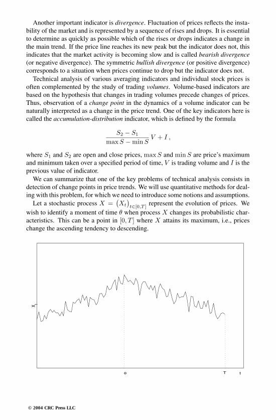
Another important indicator is divergence. Fluctuation of prices reflects the insta-bility of the market and is represented by a sequence of rises and drops. It is essentialto determine as quickly as possible which of the rises or drops indicates a change inthe main trend. If the price line reaches its new peak but the indicator does not, thisindicates that the market activity is becoming slow and is called bearish divergence(or negative divergence). The symmetric bullish divergence (or positive divergence)corresponds to a situation when prices continue to drop but the indicator does not.

Technical analysis of various averaging indicators and individual stock prices isoften complemented by the study of trading volumes. Volume-based indicators arebased on the hypothesis that changes in trading volumes precede changes of prices.Thus, observation of a change point in the dynamics of a volume indicator can benaturally interpreted as a change in the price trend. One of the key indicators here iscalled the accumulation-distribution indicator, which is defined by the formula

S2 − S1

maxS −minSV + I ,

where S1 and S2 are open and close prices, maxS and minS are price’s maximumand minimum taken over a specified period of time, V is trading volume and I is theprevious value of indicator.

We can summarize that one of the key problems of technical analysis consists indetection of change points in price trends. We will use quantitative methods for deal-ing with this problem, for which we need to introduce some notions and assumptions.

Let a stochastic process X =(Xt

)t∈[0,T ]

represent the evolution of prices. Wewish to identify a moment of time θ when process X changes its probabilistic char-acteristics. This can be a point in [0, T ] where X attains its maximum, i.e., priceschange the ascending tendency to descending.

X t

Tθ t


Then we need to choose a stopping time τ∗ adapted to the observed information,such that τ∗ is sufficiently close to θ and the values of X at these points are also closein some sense; for example, the variance of the difference Xθ −Xτ∗ is minimal. In1900 Bachelier suggested that the evolution of prices can be modelled with the helpof a standard Wiener process (Brownian motion): Xt = wt, t ∈ [0, T ].

For simplicity, let T = 1. We construct an approximation of quantity wθ usingwτ , where stopping time τ is adapted to filtration F =

(Ft

)t≥0

generated by Wienerprocess w:

Ft = σ(wt), t ≥ 0.

Let us introduce the following notation:

St := max0≤s≤t

ws ,

and

V ∗ := infτ

E(G(S1 − wτ

)),

where G is an observations cost function, and the infimum is taken over all stoppingtimes τ , i.e., over all random variables such that

ω : τ ≤ t ∈ Ft for all t ≥ 0 .

Our aim is to find an optimal stopping time τ∗, so that

V ∗ = E(G(S1 − w∗

τ

)).

The existence and structure of quantities τ∗ and V ∗ is given by the followingtheorem [43].

THEOREM 2.7

For the cost function G(x) = x2 the optimal stopping time τ∗ is defined bythe formula

τ∗ = inft ≤ 1 : St − wt ≥ z∗

√1− t

.

Here z∗ ≈ 1.12 is a solution to equation

4Φ(z)− 2 z φ(z)− 3 = 0 ,

where

Φ(z) =∫ z

−∞φ(x) dx and φ(z) =

1√2π

e−z2/2 .

In this caseV ∗ = 2Φ(z∗)− 1 ≈ 0.73 .


REMARK 2.2

1. The quantitative characteristics of the optimal stopping time are

E(τ∗) =z∗ 2

1 + z∗ 2≈ 0.55 ,

V (τ∗) =2 z∗ 4

(1 + z∗ 2) (3 + 6 z∗ 2 + z∗ 4)≈ 0.05 .

2. For an arbitrary time interval [0, T ] the optimal stopping time and priceare given by

τ∗(T ) = inft ≤ T : St − wt ≥ z∗

√T − t

and V ∗(T ) = V ∗ T ,

respectively.

PROOF (of Theorem 2.7) From the strong Markov property of theWiener process, for any stopping time τ and for any cost function G = G(x)with E

(|G(S1 − wt)|)< ∞, we have

E(G(S1 − wτ )

∣∣Fτ

)= E

(G(max

maxu≤τ

wu, maxτ<u≤1

wu

− wτ

)∣∣∣Fτ

)= E

(G(max

s, max

0≤τ≤1−twτ + x

− x))∣∣∣∣

x=wτ ,s=Sτ ,t=τ

= E(G(max

s, η + x

− x))∣∣∣∣

x=wτ ,s=Sτ ,t=τ

,

where random variableη = max

0≤τ≤1−twτ

has the following distribution

dFη(t, y) = 2φ(

y√1− t

)dy√1− t

.

Thus

E(G(S1 − wτ )

∣∣Fτ

)= G(s− x)Fη(t, s− x) +

∫ ∞

s−x

G(y) dFη(t, y)

= G(s− x) +∫ ∞

s−x

[G(y)−G(s− x)

]dFη(t, y) ,

where x = wτ , s = Sτ , t = τ .


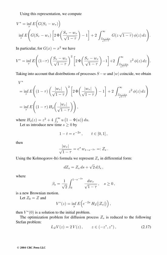
Using this representation, we compute

V ∗ = infτ

E(G(S1 − wτ )

)infτ

E

(G(Sτ − wτ )

[2Φ(Sτ − wτ√1− τ

)− 1]+ 2

∫ ∞

Sτ −wτ√1−τ

G(z√1− τ)φ(z) dz

).

In particular, for G(x) = x2 we have

V ∗ = infτ

E

((1−τ)

(Sτ − wτ√1− τ

)2 [2Φ(Sτ − wτ√1− τ

)−1]+2

∫ ∞

Sτ −wτ√1−τ

z2 φ(z) dz

).

Taking into account that distributions of processes S−w and |w| coincide, we obtain

V ∗

= infτ

E

((1− τ)

( |wτ |√1− τ

)2 [2Φ( |wτ |√

1− τ

)− 1

]+ 2

∫ ∞

Sτ −wτ√1−τ

z2 φ(z) dz

)

= infτ

E

((1− τ)H2

( |wτ |√1− τ

)),

where H2(z) = z2 + 4∫∞z

u(1− Φ(u)

)du.

Let us introduce new time s ≥ 0 by

1− t = e−2s , t ∈ [0, 1] ,

then|wτ |√1− τ

= es w1−e−2s =: Zs .

Using the Kolmogorov-Ito formula we represent Zs in differential form:

dZs = Zs ds+√2 dβs ,

where

βs =1√2

∫ 1−e−2s

0

dwτ√1− τ

, s ≥ 0 ,

is a new Brownian motion.Let Z0 = Z and

V ∗(z) = infs

E(e−2s H2

(|Zs|))

,

then V ∗(0) is a solution to the initial problem.The optimization problem for diffusion process Zs is reduced to the following

Stefan problem:LZV (z) = 2V (z) , z ∈ (−z∗, z∗) , (2.17)


V (± z∗) = H2(z∗) , V ′(± z∗) = ±H ′2(z

∗) ,

where LZ = z ddz +

d2

dz2 is generating operator of the diffusion process Zs, s ≥ 0.General solution of equation (2.17) is given by

V (z) = c1 e−z2/2 M

(3/2, 1/2; z2/2

)+ c2 z e

−z2/2 M(2, 3/2; z2/2

),

where

M(a, b;x) = 1 +a

bx+

a (a+ 1)b (b+ 1)

x2

2!+ . . .

is the hypergeometric Kummer function.Since V ∗(z) is even function, we have c2 = 0. From boundary conditions we also

have

c1 = ez∗2/2 H2(z∗)

M(3/2, 1/2; z∗2/2

) ,where z∗ is a strictly positive solution of equation

H ′2(z)

H2(z)+ z = 3 z

M(5/2, 1/2; z2/2

)M(3/2, 1/2; z2/2

) .Thus we obtain the following expression for the price V ∗(z):

V ∗(z) =

H2(z) exp

z∗2−z2

2

M(3/2,1/2;z2/2

)M(3/2,1/2;z∗2/2

) , if |z| ≤ z∗

H2(|z|) , if |z| ≥ z∗.

The corresponding stopping time is then defined as the first exit time from the ball

σ∗ = infs ≥ 0 : |Zs| ≥ z∗

with radius z∗.

The standard verification procedure can be used now to prove that these quantitiesare optimal. Then we can write solutions to the initial problem. Indeed, changingback to time t = 1 − e−2s and using the facts that Zt = wt/

√1− t and that the

distributions of S − w and |w| coincide, we obtain an expression for the optimalstopping time for the initial problem:

τ∗ = inft ≤ 1 : St − wt ≥ z∗

√1− t

.

Since evolution of prices in the problem of quickest detection of tendencies isdescribed in terms of a stochastic process, one can consider a slightly different settingof that problem. Namely, one solves a problem of quickest detection of time whenthe probabilistic characteristics of the stochastic process change. This problem isreferred to as a change point problem, and it was introduced by Kolmogorov andShiryaev.


It is convenient to specify process X in the following way:

dXt =σ dwt , if t < θr dt+ σ dwt , if t ≥ θ

.

The stopping time τ adapted to observations of process X can be interpreted as analarm time by considering the following events:

ω : τ < θ and ω : τ ≥ θ ,where the first event corresponds to a false alarm, and the second indicates that thechange point has been passed and one has to make a decision as promptly as possi-ble. One of the natural criteria for making such a decision can be formulated in thefollowing form: for a fixed c > 0,

(a) findV (c) = inf

τ

P(ω : τ < θ)+ cE

((τ − θ)+

),

where τ is a stopping time adapted to filtration(FX

t

)generated by the ob-

served price process Xt;

(b) find a stopping time τ∗ such that

V (c) = P(ω : τ∗ < θ)+ cE

((τ∗ − θ)+

).

This criterium has a clear and natural meaning: the decision to stop is made ata time when the probability of a false alarm and the average delay after the changepoint θ are minimal.

Suppose that random variable θ has an exponential a priori distribution with pa-rameter λ > 0:

P(ω : θ = 0) = π ∈ [0, 1]

P(ω : θ ≥ t | θ > 0) = e−λt .

Posterior distribution of θ is denoted

πt = P(ω : θ ≤ t | FX

t

).

It gives rise to a new statisticϕt =

πt1− πt

,

whose structure we now study.Denote Pθ the conditional distribution of X with respect to θ. Note that P0 corre-

sponds to the case when dXt = r dt+ σ dwt, and P∞ corresponds to the case whendXt = σ dwt. Introducing statistics

Lt =dP0

dP∞(t,X) ,


we can writedPθ

dP∞=

Lt

Lθ, θ ≤ t .

By Bayes’s formula we obtain

ϕt(λ) = ϕt =P(ω : θ ≤ t |FX

t

)P(ω : θ > t |FX

t

)=

π

1− πeλt

dP0

dP∞(t,X) + eλt

∫ t

0

dPθ

dP∞(t,X)λ e−λθ dθ

=π

1− πeλt Lt + λ eλt

∫ t

0

Lt

Lθe−λθ dθ .

Now, taking into account

dLt =r

σ2Lt dXt ,

and using the Kolmogorov-Ito formula, we obtain

dϕt = λ (1 + ϕt) dt+r

σ2ϕt dXt , ϕ0 =

π

1− π.

Taking into account the relationship between ϕt and πt, and using the Kolmogorov-Ito formula, we arrive at a stochastic differential equation for the posterior probabilityπt:

dπt =(λ− r

σ2π2t

)(1− πt) dt+

r

σ2πt (1− πt) dXt , π0 = π .

Now we solve the problem (a)–(b) in this Bayes’s setting with the a priori proba-bility π. Rewrite V (c) = V (c, π) in the form

V (c, π) = infτ

E

((1− πt) + c

∫ τ

0

πs ds

)= ρ∗(π) .

Consider the following innovation representation of process X:

dXt = r π dt+ σ dwt ,

where w is some new Brownian motion with respect to filtration(FX

t

).

Using this representation we can rewrite stochastic differential equation for πt inthe form

dπt = λ (1− πt) dt+r

σ2πt (1− πt) dwt .

Noting that ∫ t

0

πs ds =π0 − πt

λ+

1λ

r

σ

∫ t

0

πs (1− πs) dwt + t ,


we arrive at the following expression for the price function

V (c, π) = ρ∗(π) = infτ

E

((1 +

c

λπ)−(1 +

c

λ

)πτ + c τ

).

Thus, πt is a diffusion process generated by operator

L = a(π)d

dπ+

12b2(π)

d2

dπ2,

where a(π) = λ (1− π) and b(π) = π (1− π) r/σ.Now we can apply the standard method of solving the change point problem,

which reduces to the Stefan problem

Lρ(π) = −c π , π ∈ [0, B),ρ(B) = 1−B , π ∈ [B, 1],ρ′(B) = −1 , ρ′(0) = 0 .

A general solution of this problem depends on two unknown constants. Anotherunknown parameter is constant B, which defines the a priori unknown boundary ofthe region in this free-boundary problem. Having one boundary condition for ρ atπ = B and two conditions for derivatives ρ′(B) and ρ′(0) (conditions of smoothsewing of a solution), we can write solution in the explicit form:

ρ(π) =

(1−B∗)− ∫ B∗

πy∗(x) dx , π ∈ [0, B∗)

1− π , π ∈ [B∗, 1] ,

where

y∗(x) = −C

∫ x

0

e−Λ [G(x)−G(y)] dy

y (1− y)2

with

G(y) = logy

1− y− 1

y, Λ =

λ

r2/2σ, C =

c

r2/2σ,

and B∗ is a solution to

C

∫ B∗

0

e−Λ [G(B∗)−G(y)] dy

y (1− y)2= 1 .

The standard verification technique can be used to show that found function ρ(π)coincides with ρ∗(π), and

τ∗ = τ∗(B) = inft : πt ≥ B∗

is an optimal stopping time, such that

ρ∗(π) = E

((1− πτ∗) + c

∫ τ∗

0

πs ds

),

V (c, π) = Pπ

(ω : τ∗ < 0)+ cEπ

((τ∗ − θ)+

),


where notation Pπ and Eπ reflects the presence of an a priori distribution withP(w : θ = 0) = π.Finally, we note that the same methodology can be applied when the evolution of

prices is represented by process Xt = µ t + wt. Using Girsanov theorem, we canconstruct a new probability P ∗ such that process µ t+wt is a Brownian motion withrespect to it.


Chapter 3

Insurance Risks. Foundations ofActuarial Analysis

In this chapter we discuss insurance risks, methodologies of premium calculationsand of estimation of reserves. In particular, we focus on actuarial analysis of risksthat takes into account the investment strategies of an insurance company.

3.1 Modelling risk in insurance and methodologies ofpremium calculations

Insurance is a contract (policy) according to which one party (a policy holder)pays an amount of money (premium) to another party (insurer) in return for an obli-gation to compensate some possible losses of the policy holder. The aim of sucha contract is to provide a policy holder with some protection against certain risks.Death, sickness, disability, motor vehicle accident, loss of property, etc. are sometypical examples of such risks. Each policy contract specifies the policy term and themethod of compensation. Usually compensation is provided in the form of paymentof an amount of money. Any event specified in the policy contract that takes placeduring its term can result in such an insurance claim. If none of the events specifiedin the policy contract happen during the policy term, then the policy holder has nomonetary compensation for the paid premiums.

The problem of premium calculation is one of the key issues in the insurancebusiness: if the premium rate is too high, an insurance company will not have enoughclients for successful operation. If the premium rate is too low, the company also maynot have sufficient funds to pay all the claims.

To study this problem we need the following basic notions:

• x, the initial capital of an insurance company;

• non-negative sequence of random variables σ0 = 0 ≤ σ1 ≤ . . ., time momentsof receiving claims. Sequence Tn = σn − σn−1, n ≥ 1, represents timeintervals between claims arrivals;

• N(t) = supn : σn ≤ t is the total number of claims up to time t. It is


obviously connected with sequence (σn):ω : N(t) = n

=ω : σn ≤ t < σn−1

;

• sequence of independent identically distributed random variables (Xn), whereeach Xn represents amount of claim at time σn;

• X(t) =∑N(t)i=1 Xi is the aggregate claim amount up to time t. Usually X is

referred to as a risk process. Note that X(t) = 0 if N(t) = 0;

• denote Π(t) the total premium income up to time t ≥ 0;

• the capital of an insurance company at time t ≥ 0 is given by

R(t) = x+Π(t)−X(t) .

Naturally, we want to measure and to compare risks. The most common measureof risk in insurance is the probability of bankruptcy:

1− P(ω : R(t) ≥ 0, t ∈ [0, T ]) ,

where T is some time horizon.Next we introduce some natural assumptions regarding process N(·):1. N(0) = 0;

2. N(t) ∈ 0, 1, 2, . . . ;

3. N(t) ≤ N(t+ h).

Thus, the quantity N(t+h)−N(t) describes the number of claims received duringthe time interval (t, t+ h).

N(t)

σ0

σ1 σ

2σ

3


Usually it is assumed that process N(·) can have only unit jumps, i.e., it is notpossible to receive two or more claims simultaneously. Consider the distribution ofN(·):

pk(t) = P(ω : N(t) ≤ k) = P

(ω :

k∑i=1

Ti ≤ t <k+1∑i=1

Ti

).

Probabilities pk(t) can be explicitly computed under the additional assumption onsequence (Tn). If (Tn) is a sequence of independent identically distributed randomvariables with the distribution function

FT (x) = P(ω : Tn ≤ x) ,

then sequence (σn) is called a renewal process. A typical example of such a pro-cess is a Poisson renewal process, when (Tn) has an exponential distribution with aparameter λ > 0, and therefore the distribution of N(t) has the form

pk(t) = e−λt(λt)k

k!, k = 0, 1, . . . .

In this case E(N(t)

)= λ t, V

(N(t)

)= λ t.

For example, if λ = 2, then we have the following values of pk(t):

k t = 0.1 t = 0.2 t = 1 t = 20 0.8187 0.6703 0.1353 0.01831 0.1637 0.2681 0.2707 0.07332 0.0164 0.0536 0.2707 0.14653 0.0011 0.0072 0.1804 0.19544 0.0001 0.0007 0.0902 0.19545 0 0.0001 0.0361 0.15636 0 0 0.0120 0.10427 0 0 0.0034 0.05958 0 0 0.0009 0.02989 0 0 0.0002 0.013210 0 0 0 0.0053


0 1 2 3 4 5 6 7 8 9 100

0.1

0.2

0.3

0.4

0.5

0.6

0.7

0.8

0.9

p k(t)

k

t=0.1t=0.2t=1t=2

We will assume that claims are paid instantaneously at the time of arrival, al-though in reality there may be a time delay related to estimation of the amount ofa claim. Sometimes these delays can be rather significant, e.g., in insurance againstcatastrophic events.

The exact distribution of claims is often unknown. It is assumed that it can bedescribed by some parametric family. Hence, one of the primary tasks in modellinginsurance risks is estimating these parameters.

Here are examples of some widely used distributions

Poisson

P(ω : X = x) = e−λ

λx

x!, x = 0, 1, 2, . . . ,

is often used for modelling the number of claims;

Binomial

P(ω : X = x) = (m

x

)qx (1− q)m−x , x = 0, 1, 2, . . . ,m ,

represents the number of claims for a portfolio of m independent policies,where q is probability of receiving a claim (if m = 1, then it is called Bernoullidistribution);

Normal

P(ω : X ≤ x) = ∫ x

−∞

1√2π σ

e−(x−µ)2/2σ2dx ;

ExponentialP(ω : X ≤ x) = 1− e−λx , x ≥ 0, λ > 0 ,


has various applications, for example, models the distribution of jumps of aPoisson process with intensity λ;

Gamma

P(ω : X ≤ x) = ∫ x

0

βα

Γ(α)xα−1 e−βx dx , β > 0 ;

Papeto

P(ω : X ≤ x) = 1− ( λ

λ+ x

)α, x ≥ 0, α > 0, λ > 0 ,

has a ‘heavy’ tail, and hence is often used in modelling large claims;

Lognormal

P(ω : X ≤ x) = ∫ x

0

1√2π σ

e−(log x−µ)2/2σ2dx .

Denote

FX(t) = P(ω : X ≤ x) = P

(ω :

N(t)∑i=1

Xi ≤ x)

,

the distribution of the risk process.To compute FX(t)(x) one needs some additional assumptions. Usually processes

(Xn) and N(·) are assumed to be independent. Then we can write

FX(t)(x) = P(ω : X ≤ x) = ∞∑

k=0

pk(t)F ∗kX (x) ,

whereF ∗kX (x) = P

(ω : X1 + . . .+Xk ≤ x) .Premium calculation or determination of process Π(t) is one of the most essential

and complex tasks of an insurer. Premium flow must guarantee payments of claims,but on the other hand, premiums must be competitive. One of the most widely usedways of computing Π on interval [0, t] is given by

Π(t) = (1 + θ)E(N(t)

)E(X),

where X is a random variable with the same distribution as Xi, and θ is the securityloading coefficient. This formula says that the average premium income should begreater than the average aggregate claims payment. If they are equal, then suchpremium is called net-premium and the method of its computing is referred to asequivalence principle.

The bonus-malus system is an example of a different approach to premium calcu-lations. In this case, all policy holders are assigned certain ratings according to their


claims history, and they can be transferred from one group to another. This systemis typically used by the motor vehicle insurance companies.

Calculation of adequate premium consists in construction of process Π(t) givenFX(t), the distribution function of the risk process. In this case we will write Π(FX)or simply Π(X).

Process Π has the following properties

• Π(a) = a for any constant a if θ = 0;

• Π(aX) = aΠ(X) for any constant a;

• Π(X + Y ) ≤ Π(X) + Π(Y );

• Π(X + a) = Π(X) + a for any constant a;

• if X ≤ Y , then Π(X) ≤ Π(Y );

• for any p ∈ [0, 1] and any random variable Z

Π(X) = Π(Y )

implies that

Π(pFX + (1− p)FZ

)= Π

(pFY + (1− p)FZ

).

We list some widely used actuarial principles of premium calculations:

Expectation principle

Π(X) = (1 + a)E(X), a > 0;

Variance principleΠ(X) = E(X) + a V (X);

Standard deviation principle

Π(X) = E(X) + a√V (X);

Modified variance principle

Π(X) =

E(X) + aV (X)/E(X) , E(X) > 0

0 , E(X) = 0 ;

Exponential utility principle

Π(X) =logE(eaX)

a;


Quantile principleΠ(X) = F−1

X (1− ε);

Absolute deviation principle

Π(X) = E(X) + a κX where κX = E(∣∣X − F−1

X (1/2)∣∣);

Zero utility principleE(υ(Π(X)−X)

)= υ(0) ,

where υ is a given utility function.

Note that the exponential principle is a particular case of the zero utility principlewith

υ(x) =1− e−ax

a.

The notion of risk is the key ingredient of insurance theory and practice. Riskexposure gives rise to insurance companies that manage risks and provide some pro-tection against these risks to their clients. Reinsurance companies provide similarservices to insurance companies. There are several approaches to modelling the riskprocess.

Consider a portfolio that consists of n policy contracts with claim payments(‘risks’) X1, . . . , Xn being independent non-negative random variables. Then therisk process

X ind =n∑i=1

Xi ,

has distribution FX1 ∗ . . . ∗ FXn . This model of risk is referred to as individual.Suppose that an insurance company issues n insurance contracts that terminate at

some time t, e.g., in one year’s time. Each contract allows no more than one claim.Claim payments X1, . . . , Xn are non-negative random variables. The total amount ofclaims incurred over this period is represented by the risk process X ind =

∑ni=1 Xi.

It is also assumed that all claims are payable at the termination time. Therefore, theprobability of bankruptcy (or insolvency) is given by

P(ω : X ind > x+Π) ,

where x is the initial capital of the company and Π is the premium income.Thus, the model of individual risk is based on the following assumptions:

• time horizon is relatively short;

• number of insurance contracts is deterministic and fixed;

• premiums are payable at the time of contracts issue;

• the distribution of claim payments is known.


Example. Consider a model of individual risk with a sufficiently large number ofinsurance contracts. Since exact calculation of probability of bankruptcy is techni-cally complicated, we use the Central Limit Theorem for its approximation.

Using the net-premium principle we have that Π = X ind. Then we compute theprobability of bankruptcy:

P(ω : X ind > Π) = P

(ω : X ind − E(X ind) > 0)= P

(ω :

X ind − E(X ind)√V (X ind)

> 0)

≈ 1− Φ(0) = 0.5 ,where

Φ(x) =1√2π

∫ x−∞

e−y2/2 dy .

This means that the net-premium principle cannot be used in this situation.The standard deviation principle gives

Π = E(X ind) + a√

V (X ind)

and

P(ω : X ind > Π) = P

(ω :

X ind − E(X ind)√V (X ind)

> a

)≈ 1− Φ(a) .

In this case, for any fixed level of risk ε, we can find a parameter a such that Φ(a) =1− ε, so that the probability of bankruptcy is

P(ω : X ind > Π) ≈ ε .

Now we consider a situation when N , the number of possible claims, is unknown.We can single out two types of insurance contracts: static and dynamic. In the staticcase, claims are payable at the terminal time, and therefore N is an integer-valuedrandom variable. In the dynamic model, N = N(t) is a stochastic process thatcounts the number of claims incurred during the time interval [0, t]. Both these mod-els of risk are referred to as collective. The risk process has the form

Xcol =N∑i=1

Xi ,

where claims amounts Xi are positive and independent of N . Clearly, the collectivemodel of risk is more realistic than the individual model, and it gives more flexibilityin managing risk for an insurance company.

Some essential differences between the two models are summarized in the follow-ing table.


individual model collective model

n, the number of insurance the process of receiving claimscontracts is known a priori is represented by a stochasticand all claims are payable processat the same timeeach contract admits no more there is no restrictions onthan one claim number of claims per contractall claims are assumed to be it is assumed that the amountsindependent of incurred claims are independent

WORKED EXAMPLE 3.1Suppose an insurance company issues 1-year contracts. All policy holders aredivided into four groups:

k qk bk nk

1 0.02 1 5002 0.02 2 5003 0.1 1 3004 0.1 2 500

Here nk is the number of policy holders in group k, qk is the probability ofmaking a claim by a member of this group and bk is the amount of the cor-responding claim. Using normal approximation, find the value of the securityloading coefficient that will reduce the probability of insolvency to 0.05.

SOLUTION The total number of policy holders is 1800, so the totalamount of claims is

S = X1 + . . .+X1800 .

We will find parameter θ from the equation

P(ω : S ≤ (1 + θ)E(S)) = 0.95 ,

which can be written in the form

P

(ω :

S − E(S)√V (S)

≤ θ E(S)√V (S)

)= 0.95 .

Since the total number of policy holders is reasonably large, then the quantity(S − E(S)

)/√V (S) can be accurately approximated by a standard normal

distribution. Hence we obtain the equation

θ E(S)√V (S)

≈ 1.645 .


The following table contains expectations µk = bk qk and variances σ2k =

b2k qk (1− qk) for each policy.

k qk bk µk σ2k nk

1 0.02 1 0.02 0.0196 5002 0.02 2 0.02 0.0784 5003 0.1 1 0.1 0.09 3004 0.1 2 0.2 0.36 500

Thus

E(S) =1800∑i=1

E(Xi) =4∑k=1

nk µk = 160 ,

V (S) =1800∑i=1

V (Xi) =4∑k=1

nk σ2k = 256 ,

and

θ ≈ 1.645

√V (S)E(S)

= 1.64516160

= 0.1645 .

Note that situations where the number of claims is a random variable are typicalfor life insurance, and they are studied in Section 3.4.

Another example of a collective risk model is the Cramer-Lundberg model. Theclaims flow is modelled here as a Poisson process N(t) with intensity λ, and claimsamounts are independent random variables that are also independent of N(t). Thepremium income is a linear function of time t: Π(t) = c t. The risk process

X(t) =N(t)∑i=1

Xi

is a compound Poisson process. It turns out that if the initial probability P thatdescribes the distribution of claims is replaced by an equivalent probability Q un-der which X is also a compound Poisson process, then applying the equivalenceprinciple with respect to this new probability Q, we obtain all the above mentionedtraditional principles of premium calculations.

Indeed, define a positive process

Mβt = exp

Xβ(t)− λ tEP

(expβ(X1) − 1

), Mβ

0 = 1, t ∈ [0, T ] ,

where Xβ(t) =∑N(t)k=1 β(Xk), function β : R+ → R is such that

EP(expβ(X1)

)< ∞, and the expectation EP is taken with respect to proba-

bility P .


Process Mβ is a martingale since for s ≤ t we have

EP(Mβt |Fs

)=Mβ

s EP(expXβ(t)−Xβ(s)) e−λ(t−s) EP ( expβ(X1) − 1

)=Mβ

s .

Hence, EP(Mβt

)= 1, and for each such function β one can define new probability

Q with density Mβt . Note that any other probability Q under which the risk process

X(t) is a compound Poisson process must have exactly the same structure with someappropriate function β (for details see [31]).

Thus, we can use this function β and the corresponding probability Q for calcu-lating premium. This calculation is based on the condition that the difference

X(t)− c t

between the total amount of claims and the total premium income is a martingalewith respect to Q. This agrees with the equivalence principle in insurance and withthe no-arbitrage principle in finance.

So we obtain thatc = EQ

(X(1)

),

and since X(t) is a compound Poisson process, then

EQ(X(1)

)= EQ

(N(1)

)EQ(X1

),

where

EQ(N(1)

)= λEP

(expβ(X1)

)EQ(X1

)= EP

(X1 expβ(X1)

)/EP(expβ(X1)

).

Finally, we deducec = λEP

(X1 expβ(X1)

).

Choosing appropriately β, we then obtain all the traditional actuarial principles ofpremium calculations. For example, the expectation principle corresponds to β(x) =ln(1 + a), and we have

c = λEP(X1 expβ(X1)

)= λEP

(X1 (1 + a)

)= (1 + a)EP

(X1

)= Π(X) .

3.2 Probability of bankruptcy as a measure of solvencyof an insurance company

Consider a collective risk model with a binomial process N(t) representing thetotal number of claims up to time t:

N(0) = 0, N(t) = ξ1 + . . .+ ξt, t = 1, 2, . . . ,


where (ξi)∞i=1 is a sequence of independent Bernoulli random variables such that

P(ω : ξi = 1

)= q and P

(ω : ξi = 0)= 1− q .

Sequence of independent identically distributed random variables (Xi)∞i=1 withvalues in the set of all natural numbers N, represents the amounts of claims. Denote

fn = P(ω : Xi = n) , f(z) =

∞∑n=1

fn zn and µ = E(Xi)

the distribution, the generating function and the expectation of (Xi)∞i=1, respectively.Assuming that sequences (Xi)∞i=1 and (ξi)∞i=1 are independent, let

X(k) = X1 ξ1 + . . .+Xk ξk

andgn(k) = P

(ω : X(k) = n) , n = 0, 1, 2, . . . .

Then the sum

Gn(k) =n∑m=0

gn(k) , n = 1, 2, . . .

is the distribution function of X(k), the sum of independent identically distributedrandom variables Xl ξl, l = 1, . . . k with generating functions

∞∑i=0

P(ω : Xl ξl = i) zi = 1− q + q

∞∑i=1

P(ω : Xl = i) zi

= 1− q + q f(z) .

Thereforeg(z, k) =

[1− q + q f(z)

]k.

is the generating function of X(k).Consider a stochastic sequence

R(k) = x+ k −X(k), k = 1, 2, . . . , R(0) = x ∈ 0, 1, 2, . . . ,which represents the capital of an insurance company, where x is the initial capital, kis premium income (i.e., at each time k = 1, 2, . . . the company receives the premiumof 1). This model is referred to as a compound binomial model.

Functions

φ(x, k) = P(ω : R(j) ≥ 0, j = 0, 1, . . . , k) and φ(x) = lim

k→∞φ(x, k),

are called the probabilities of non-bankruptcy (probabilities of solvency) on a finiteinterval [0, k] and infinite interval [0,∞), respectively.

Clearly, knowing the analytical expressions for this functions, one can estimatethe solvency of the company.


To find an expression for φ(x, k) we assume that the initial capital is x− 1, wherex ≥ 1. We also accept that the probability of solvency of a company with negativeinitial capital is equal to zero. Then for any integers k and x we have the followingrecurrence relation:

φ(x− 1, k) = E(φ(R(1), k − 1))

= (1− q)φ(x, k − 1) + qx∑y=1

φ(x− y, k − 1) fy .

Further, using the technique of generating functions, we obtain the following ex-pression for the probability of solvency of a company with zero initial capital (fordetails see Section 3.2.2: Mathematical appendix 1):

φ(0, k) =∑km=0(k + 1−m) gm(k + 1)

(1− q) (k + 1), k = 0, 1, . . . .

If the initial capital x = 1, 2, . . ., then we have

φ(x, k) = Gx+k(k)− (1− q)k −1∑m=0

φ(0, k − 1−m) gx+m+1(m) ,

for k = 1, 2, . . . (see Section 3.2.3: Mathematical appendix 2).In the case of the infinite time interval [0,∞), we use the following formula from

Section 3.2.4: Mathematical appendix 3

φ(0, k) =1− q µ

1− q+

∑∞m=k+1

(1−Gm(k + 1)

)(1− q) (k + 1)

.

Taking limit as k → ∞, we obtain (see Section 3.2.4: Mathematical appendix 3)

φ(0) =1− q µ

1− q.

Now we establish a relation between the initial capital and probabilistic charac-teristics of claims, which guarantees the solvency of an insurance company over theinfinite period of time with the probability that corresponds to a chosen (fixed) levelof risk ε > 0:

φ(0) ≥ 1− ε .

This implies

µ ≤ 1− ε+ε

q.

The case when the initial capital is greater than zero is illustrated by the followingexample.


WORKED EXAMPLE 3.2Consider function

φ(z) =∞∑x=0

φ(x) zx .

Let Xi ≡ 2, then f(z) = z2 and µ = 2.Find values of the initial capital that guarantee that the probability of insol-

vency is less than the chosen level of risk.

SOLUTION Note that function φ(z) can be written in the form (seeSection 3.2.5: Mathematical appendix 4):

φ(z) =1

1− z

1− q µ

1− q µ b(z),

where

b(z) =g(z, 1)− 1q µ (z − 1) =

f(z)− 1µ (z − 1) .

In our case b(z) = (1 + z)/2, hence

φ(z) =1

1− z

q (1− q)−1

1− q z (1− q)−1.

Expanding φ(z) in powers of Z, we obtain

φ(x) = 1−(

q

1− q

)x+1

.

Positivity of the security loading coefficient 1− q µ > 0 implies

q <12

andq

1− q< 1, .

The following table and figure give probabilities of insolvency for four dif-ferent values of q with accuracy 0.0001.

Initial capital q = 0.1 q = 0.2 q = 0.4 q = 0.490 0.1111 0.25 0.6667 0.96081 0.0123 0.0625 0.4444 0.92312 0.0014 0.0156 0.2963 0.88693 0,0002 0.0039 0.1975 0.85214 0 0.001 0.1317 0.81875 0 0.0002 0.0878 0.78666 0 0.0001 0.0585 0.75587 0 0 0.0390 0.72618 0 0 0.0260 0.69769 0 0 0.0173 0.670310 0 0 0.0116 0.6440


0 1 2 3 4 5 6 7 8 9 100

0.1

0.2

0.3

0.4

0.5

0.6

0.7

0.8

0.9

1

Prob

abilit

y of

Inso

lvenc

y

Initial Capital

q=0.1q=0.2q=0.4q=0.49

For a given level of risk ε we solve the following inequality for x

φ(x) > 1− ε .

We have

x >ln(ε)

ln(q/(1− q)

) − 1 .The next table and figure give the minimal values of the initial capital x

for various values of q and ε.

q ε = 0.05 ε = 0.03 ε = 0.010.05 1 1 10.1 1 1 20.15 1 2 20.2 2 2 30.25 2 3 40.3 3 4 50.35 4 5 70.4 7 8 110.45 14 17 22


0.05 0.1 0.15 0.2 0.25 0.3 0.35 0.4 0.450

2

4

6

8

10

12

14

16

18

Initia

l Cap

ital

q

ε=0.05ε = 0.03

3.2.1 Cramer-Lundberg model

Let (Ω,F , P ) be a probability space. Consider a Poisson process N(t), t ≥ 0,with intensity λ: N(0) = 0, E(N(t)) = λt, and an independent of N sequence(Xi)∞i=1 of independent identically distributed random variables with expectation µand distribution function F (x), F (0) = 0.

The claims flow (number of claims received up to time t) is represented by thePoisson process N(t). The amounts of these claims are represented by sequence(Xi)∞i=1. The premium income of an insurance company is given by Π(t) = ct,where c is a constant. If x is the initial capital of the company, then the dynamics ofthe company’s capital is given by

R(t) = x+ c t−N(t)∑i=1

Xi .

Since N(t) and (Xi)∞i=1 are independent, then the expectation of the risk processX(t) =

∑N(t)i=1 Xi is E

(X(t)

)= λ t µ. Setting the security loading coefficient at

θ =Π(t)

E(X(t))− 1 = c− λµ

λµ,

we obtain c = (1 + θ)λµ.Now we compute the probability of solvency

φ(x) = P(ω : R(t) ≥ 0, R(0) = x, t ≥ 0) .


First we investigate smoothness of function φ(x) assuming that the distributionfunction F (x) has density f(x). Since bankruptcy cannot occur prior time T1, whenthe Poisson process N has its first jump, then we can write

φ(x) = E(φ(x+ c T1 − x1)

)=∫ ∞

0

λ e−λs∫ x+cs

0

φ(x+ c s− y) f(y) dy ds .

Making a substitution q = x− y, we can rewrite the latter equality in the form

φ(x) =∫ ∞

0

λ e−λs∫ x−cs

φ(q + c s) f(x− q) dq ds .

Thus, if F (y) ∈ Cn[0,∞), then φ(x) ∈ Cn−1[0,∞). In further discussion weassume F (y) ∈ C3[0,∞).

Using properties of the Poisson process and the formula for total probability, weobtain

φ(x) = φ(x+ c∆t)[1− λ∆t+ o(∆t)

]+λ∆t

∫ x+c∆t0

φ(x+ c∆t− y) dF (y) + o(∆t) .

By Taylor’s formula we also have

φ(x) =[φ(x) + c φ′(x)∆t

] [1− λ∆t+ o(∆t)

]+λ∆t

∫ x+c∆t0

φ(x+ c∆t− y) dF (y) + o(∆t) ,

hence

φ(x)[λ∆t+ o(∆t)

]= c φ′(x)∆t

[1− λ∆t+ o(∆t)

]+λ∆t

∫ x+c∆t0

φ(x+ c∆t− y) dF (y) + o(∆t) .

Dividing the latter equality by ∆t and taking limits as ∆t → 0, we obtain

φ(x)λ = c φ′(x) + λ

∫ x0

φ(x− y) dF (y) . (3.1)

In the case of an exponential distribution function F , it is not difficult to find anexplicit solution of this equation. Indeed, if F (y) = 1 − e−x/µ, then equation (3.1)is reduced to

φ(x)λ = c φ′(x) + λ

∫ x0

φ(x− y)1µe−y/µ dy .


Differentiating and integrating by parts, we obtain

λφ′(x) = c φ′′(x) +λ

µφ(0) + λ

∫ x0

φ′x(x− y)

1µe−y/µ dy

= c φ′′(x) +λ

µφ(0)− λ

∫ x0

1µe−y/µ dφ(x− y)

= c φ′′(x) +λ

µφ(x) + λ

∫ x0

φ(x− y)1µde−y/µ

= c φ′′(x) +λ

µφ(x)− 1

µ

[λ

∫ x0

φ(x− y)1µe−y/µ dy

]

= c φ′′(x) +λ

µφ(x) +

c

µφ′(x)− λ

µφ(x)

= c φ′′(x) +c

µφ′(x) .

Thus we arrive at the following differential equation

φ′′(x) + φ′(x)[1µ− λ

c

]= 0 ,

whose general solution is of the form

φ(x) = B +A expx

[λ

c− 1

µ

],

where A and B are some constants. The inequality

λ

c<1µ

can be written asλµ− c < 0 ,

which reflects the positivity of θ, and therefore φ(∞) = B.Unknown constants A and B can be found from the following relations

1. φ(∞) = 1;

2. Substituting x = 0 into equation (3.1):

φ(x)λ = c φ′(x) + λ

∫ x0

φ(x− y) dF (y)

impliesφ(0)λ = c φ′(0) .


Thus we arrive at the following expression

φ(x) = 1− λµ

cexp

x

[λ

c− 1

µ

]= 1− 1

1 + θexp

− θ x

(1 + θ)µ

.

In general, for an arbitrary distribution function F , it may be difficult to find anexplicit expression for φ. In this case one can look for various estimates of ψ(x) =1 − φ(x), the probability of insolvency. The main result here is usually referred toas the Cramer-Lundberg inequality:

ψ(x) ≤ e−Rx , (3.2)

where R is a positive solution to the equation

λ+ c r = λ

∫ ∞

0

er x dF (x) .

Note that so far we have dealt with the classical insurance models, where one doesnot take into account the investment strategies of an insurance company.

3.2.2 Mathematical app endix 1

Consider equation

φ(x− 1, k) = E(φ(X1, k − 1)) (3.3)

= (1− q)φ(x, k − 1) + qx∑y=1

φ(x− y, k − 1) fy ,

and

φ1(z, k) =∞∑x=0

φ(x, k) zx ,

the generating function of(φ(x, k)

)∞x=0

.Multiplying equation (3.3) by zx, and summing in x from 1 to ∞, we obtain

z φ1(z, k) = (1− q)[φ1(z, k − 1)− φ(0, k − 1)

]+q φ1(z, k − 1) f(z)

orz φ1(z, k) = g(z, 1) φ1(z, k − 1)− (1− q)φ(0, k − 1) . (3.4)

Introduce two auxiliary functions:

φ(z, t) =∞∑k=0

φ(z, k) tk =∞∑k=0

∞∑x=0

φ(z, k) zx tk


and

φ0(t) =∞∑k=0

φ(0, k) tk . (3.5)

Multiplying equation (3.4) by tk, and summing in k from 1 to ∞, we obtain

z φ(z, k)− z φ1(z, 0) = t g(z, 1) φ(z, k)− t (1− q) φ0(t) . (3.6)

From the definition of function φ we have that φ(x, 0) = 1 for all x = 0, 1, 2, . . . .Hence

φ1(z, 0) =1

1− zfor |z| < 1 .

Then equation (3.6) can be written in the form

φ(z, k)[z − t g(z, 1)

]=

z

1− z− t (1− q) φ0(t) . (3.7)

Fix t with |t| < 1. Consider function

F (z) := z − t g(z, 1) ,

then

F (0) = 0 and F (1) = 1− t[1− q + q

∞∑n=1

fn

]= 1− t > 0 .

Also

F ′(z) = 1− t q∞∑n=1

n fn zn−1 > 1− q

∞∑n=1

n fn zn−1 > 1− q µ > 0 .

The inequality 1 − q µ > 0 is equivalent to positivity of the security loadingcoefficient, and we assume that it is the case.

Thus, for each fixed t with |t| < 1 the equation

z = t g(z, 1) (3.8)

has a unique root z = z(t) ∈ (0, 1). Therefore function z(t), |t| < 1, is a solutionto (3.8).

Now, for any analytic function h with h(0) = 0, we have

h(z(t)

)=

∞∑n=1

tn

n!dn−1

dsn−1

[h′(s)

(g(s, 1)

)n]∣∣∣∣s=0

, (3.9)

where z(t) is a solution of (3.8). Note that(g(s, 1)

)n = g(s, n).If h(z) = z, then the solution to (3.8) has the form

z(t) =∞∑n=1

tn

n!g(n− 1, n) ,


where

g(n− 1, n) = 1(n− 1)!

dn−1

dsn−1g(s, n)

∣∣∣∣s=0

Substituting h(z) = z/(1− z) into (3.9), we obtain

z(t)1− z(t)

=∞∑n=1

tn

n!dn−1

dsn−1

g(s, n)(1− s)2

∣∣∣∣s=0

. (3.10)

For s with |s| < 1, we have

g(s, n)(1− s)

≡∑∞k=0 gk(n) s

k

(1− s)

=[g0(n) + g1(n) s+ g2(n) s2 + . . .

]×[1 + s+ s2 + . . .

]= g0(n) + s

[g1(n) + g0(n)

]+ s2

[g2(n) + g1(n) + g0(n)

]+ . . .

+sk[gk(n) + gk−1(n) + . . .+ g0(n)

]+ . . . ,

so the coefficient in front of sk is

k∑m=0

gm(n) = Gk(n) .

Similarly, for s with |s| < 1, we obtain that the coefficient in front of sk in theexpansion

g(s, n)(1− s)2

≡ g(s, n) (1− s)−1

(1− s)

is equal∑km=0 Gm(n).

Thus we can write (3.10) in the form

z(t)1− z(t)

=∞∑n=1

[n−1∑m=0

Gm(n)

]tn

n!. (3.11)

If we substitute z = z(t) in (3.7), then the left-hand side of this equation vanishes,so we can find an expression for φ0(t):

φ0(t) =z(t)

t (1− q)(1− z(t)

) ,which in view of (3.11) becomes

φ0(t) =1

1− q

∞∑k=0

tk

k + 1

[k∑m=0

Gm(k + 1)

].


Since representation of φ0(t) in form (3.5) is unique, then

φ0(0, k) =∑km=0 Gm(k + 1)(1− q) (k + 1)

, k = 0, 1, . . . . (3.12)

Finally, taking into account that

k∑m=0

Gm(k + 1) =k∑m=0

(k + 1−m) gm(k + 1) ,

we write

φ0(0, k) =∑km=0(k + 1−m) gm(k + 1)

(1− q) (k + 1), k = 0, 1, . . . .


In the case when the initial capital is greater than zero, equation (3.7) implies

φ(z, t) =

(1

1− z− 1− q

zt φ0(t)

)/(1− t

g(z, 1)z

). (3.13)

To represent the right-hand side of this equality as a series in powers of t, we write(1

1− z

)/(1− t

g(z, 1)z

)=

11− z

(1 + t

g(z, 1)z

+ t2g2(z, 1)

z2+ . . .

)

=1

1− z

(1 + t

g(z, 1)z

+ t2g(z, 2)z2

+ . . .+ tkg(z, k)zk

+ . . .

)

=∞∑k=0

tkg(z, k)(1− z) zk

,

and(1− q

zt φ0(t)

)/(1− t

g(z, 1)z

)=

∞∑k=0

1− q

zφ0(0, k) tk+1

∞∑m=0

tmg(z,m)zm

=∞∑l=1

tl al ,

where

al = (1− q)l−1∑m=0

g(z,m)φ0(l −m− 1) z−m−1 .


Substituting these in (3.13) we equate the coefficients in front of tk, k ≥ 1:

φ1(z, k) =g(z, k)(1− z) zk

− (1− q)k−1∑m=0

g(z,m)φ0(k −m− 1) z−m−1

or

zk φ1(z, k) =g(z, k)(1− z)

− (1− q)k−1∑m=0

g(z,m)φ0(k −m− 1) zk−m−1 . (3.14)

If k = 0, then (3.13) reduces to

φ1(z, 0) =∞∑x=0

φ(x, 0) zx =∞∑x=0

zx =1

1− z.

Noting that

zk φ1(z, k) =∞∑j=0

φ(j, k) zj+k ,

and

g(z, k)(1− z)

=∞∑i=0

gi(k) zi∞∑j=0

zj

=[g0(k) + g1(k) z + g2(k) z2 + . . .

]×[1 + z + z2 + . . .

]= g0(k) + z

[g1(k) + g0(k)

]+ z2

[g2(k) + g1(k) + g0(k)

]+ . . .

=∞∑i=0

Gi(k) zi ,

and

(1− q)k−1∑m=0

g(z,m)φ0(k −m− 1) zk−m−1

= (1− q)k−1∑m=0

φ(0, k −m− 1)∞∑j=0

zj+k−m−1 gj(m) ,

we can rewrite (3.13) in the form

∞∑j=0

zj+k φ(j, k) =∞∑i=0

Gi(k) zi

−(1− q)k−1∑m=0

φ(0, k −m− 1)∞∑j=0

zj+k−m−1 gj(m) .


Changing summation indices to i = j+k in the first sum and to i = j+k−1−min the last sum, we obtain

∞∑i=0

zi φ(i− k, k) =∞∑i=0

Gi(k) zi

−(1− q)k−1∑m=0

φ(0, k −m− 1)∞∑

i=k−1−mzi gi+m+1−k(m) .

We rearrange the last term in the latter relation:

∞∑i=0

zi φ(i− k, k) =∞∑i=0

Gi(k) zi

−(1− q)k−1∑m=0

k−1∑i=k−1−m

zi φ(0, k −m− 1) gi+m+1−k(m)

−(1− q)k−1∑m=0

∞∑i=k

zi φ(0, k −m− 1) gi+m+1−k(m) ,

and change the order of summation:

∞∑i=0

zi φ(i− k, k) =∞∑i=0

Gi(k) zi

−(1− q)k−1∑i=0

zik−1∑

m=k−1−iφ(0, k −m− 1) gi+m+1−k(m)

−(1− q)∞∑i=k

zik−1∑m=0

φ(0, k −m− 1) gi+m+1−k(m) .

Equating coefficients in front of zi, we have

φ(i− k, k) = Gi(k)− (1− q)k−1∑m=0

φ(0, k −m− 1) gi+m+1−k(m) ,

for i ≥ k ≥ 1. In other words, for x = 0, 1, . . . and k = 1, 2, . . .

φ(x, k) = Gx+k(k)− (1− q)k−1∑m=0

φ(0, k −m− 1) gx+m+1(m) .



Equation (3.12) implies

φ(0, k) =

∑km=0

[1− (1−Gm(k + 1)

)](1− q) (k + 1)

=k + 1−∑k

m=0

(1−Gm(k + 1)

)(1− q) (k + 1)

=k + 1− (k + 1) q µ+∑∞

m=k+1

(1−Gm(k + 1)

)(1− q) (k + 1)

.

Here we used the relation

∞∑m=0

(1−Gm(k + 1)

)=(1−G0(k + 1)

)+(1−G2(k + 1)

)+ . . .

= P(ω : X(k + 1) > 0)+ P

(ω : X(k + 1) > 1)+ . . .

=∞∑j=1

∞∑i=j

P(ω : X(k + 1) = i)

= E(X(k + 1)

)= (k + 1) q µ .

This latter relation also implies the convergence of the series

∞∑m=0

(1−Gm(k + 1)

)since the sequence of its partial sums is monotonically increasing and it is boundedfrom above by (k + 1) q µ.

Thus, the probability of non-bankruptcy on [0, k] has the following analytical form

φ(0, k) =1− q µ

1− q+

∑∞m=k+1

(1−Gm(k + 1)

)(1− q) (k + 1)

.

An expression for the probability of non-bankruptcy on an infinite interval can beobtained directly from (3.1) by passing to the limit as k → ∞:

φ(j) = (1− q)φ(j + 1) + q E(φ(j + 1−X1)

), j = 0, 1, 2, . . . ,

or

φ(j + 1)− φ(j) = q[φ(j + 1)− E

(φ(j + 1−X1)

)], j = 0, 1, 2, . . . .

Summing in j from 0 to k − 1, we obtain

φ(k)− φ(0) = q

[k∑j=1

φ(j)− E

( k∑j=1

φ(j −X1))]

, k = 1, 2, . . .


or

φ(k)−(1−q)φ(0) = q

[k∑j=1

φ(j)−E

( k∑j=1

φ(j−X1))]

, k = 1, 2, . . . (3.15)

Introduce function

1+(j) :=

1 , j = 0, 1, 2, . . .

0 , j = −1,−2, . . . .

For a pair of integer-valued functions f and g we define their convolution:

(f ∗ g)(j) := ∞∑

i=−∞f(j − i) g(i) .

If f(i) = g(i) = 0 for i = −1,−2, . . ., then

(f ∗ g)(j) = j∑

i=0

f(j − i) g(i) .

Now, since

k∑j=0

φ(j) =(φ ∗ 1+

)(k) ,

k∑j=1

φ(j −X1) =k∑j=0

φ(j −X1) =(φ ∗ 1+

)(k −X1) ,

then we can rewrite equation (3.15) in the form

φ(k)− (1− q)φ(0) = q[(φ ∗ 1+

)(k)− E

((φ ∗ 1+

)(k −X1)

)](3.16)

= q[(φ ∗ 1+

)(k)− (φ ∗ 1+ ∗ f)(k)]

k = 1, 2, . . . ; f(n) = fn .

Since f(0) = 0, then (3.16) also holds for k = 0. Now we can extend (3.16) to allintegers k:

φ(k)− (1− q)φ(0) 1+(k) = q[(φ ∗ 1+

)(k)− (φ ∗ 1+ ∗ f)(k)] . (3.17)

Introduce function

δ(j) :=1 , j = 00 , j = 0 .


Then (3.17) can be written in the form

φ(k) ∗[δ(k)− q

[1+(k) ∗

(δ(k)− f(k)

)]]= c 1+(k) ,

where c = (1− q)φ(0).A solution to this equation can be written in the form of the following Neumann

series

φ(k) = c∞∑n=0

qn[(δ(k)− f(k)

)∗n ∗ 1∗(n+k)+ (k)],

where g∗0 = δ, g∗n = g∗(n−1) ∗ g, n = 1, 2, . . . .If k → ∞, then (3.16) gives

1− (1− q)φ(0) = q∞∑

j=−∞

[1+(j)−

(1+ ∗ f)(j)]

= q∞∑j=0

[1− P

(ω : X1 ≤ j)] = q µ .

Hence

φ(0) =1− q µ

1− q.


Introduce function

φ(z) :=∞∑x=0

φ(x) zx .

Taking into account

limt1

(t− 1) φ(z, t) = limt1

∞∑k=0

φ1(z, k) tk (1− t)

= limt1

[φ1(z, 0) (1− t) + φ1(z, 1) t (1− t) + . . .+ φ1(z, k) tk (1− t) + . . .

]= limt1

[φ1(z, 0) + t

(φ1(z, 1)− φ1(z, 0)

)+ . . .

]= φ1(z,∞) ≡ φ(z)

and equation (3.13), we obtain

φ(z) = limt1

(t− 1) φ(z, t) = − 1− q

z − g φ(z, 1)limt1

(t− 1) φ0(t)

=1− q µ

g(z, 1)− z=

11− z

1− q µ

1− q µ b(z),


where

b(z) =g(z, 1)− 1q µ (z − 1) =

f(z)− 1µ (z − 1) .

Also note that

φ(x) =dxφ(z)dzx

φ(z)x!

∣∣∣∣z=0

.

3.3 Solvency of an insurance company and investmentp ortfolios

As in Chapter 1, we consider a binomial (B,S)-market. The dynamics of thismarket are described by equations

∆Bn = r Bn−1, B0 > 0∆Sn = ρn Sn−1, S0 > 0, n ≤ N ,

where r ≥ 0 is a constant rate of interest with −1 < a < r < b, and profitabilities

ρn =b with probability p ∈ [0, 1]a with probability q = 1− p

, n = 1, . . . , N ,

form a sequence of independent identically distributed random variables.Suppose that an insurance company with the initial capital x = R0 forms an

investment portfolio (β1, γ1) at time n = 0, so that

R0 = β1 B0 + γ1 S0 .

At time n = 1 the capital of the company is

R1 = β1 B1 + γ1 S1 + c− Z1 ,

where c is the premium income and Z1 is a non-negative random variable repre-senting total claims payments during this time period. This capital is reinvested intoportfolio (β2, γ2):

R1 = β2 B1 + γ2 S1 .

At any time n we have

Rn = βnBn + γn Sn + c− Zn ,

where predictable sequence π = (βn, γn)n≥0 is an investment strategy and Zn isa non-negative random variable representing total claims payments during the timestep from n − 1 to n. The distribution function of Zn is denoted FZn ≡ FZ . Itis assumed that sequence (Zn)n≥0 of independent identically distributed randomvariables is also independent of the dynamics of market assets B and S.


Thus, the dynamics of the capital of the insurance company have the form

Rn+1 = βnBn+1 + γn Sn+1 + c− Zn+1

= Rn (1 + r) + γn Sn (ρn+1 − r) + c− Zn+1 .

As we discussed in the previous section, the probability of bankruptcy (or insol-vency)

P(ω : Rn < 0 for some n ≥ 0)

is one of the typical measures used in the insurance risk management. Now we studythis measure taking into account the investment strategies of an insurance company.

We start with the case when a company invests only in the non-risky asset B. Inthis case

Rn+1 = Rn (1 + r) + c− Zn+1 .

First we compute the probability of insolvency over the finite time interval [0, k]:

ψk(R0) = P(ω : Rn < 0 for some n ≤ k) .

Note that ψ is an increasing function of k and R0.The probability of insolvency after one time step is given by

ψ1(R0) = P(ω : R1 < 0) = P

(ω : R0 (1 + r) + c− z1 < 0)= P

(ω : z1 > R0 (1 + r) + c) = 1− Fz(R0(1 + r) + c

).

The probability of insolvency after two steps is

ψ2(R0) = P(ω : R1 < 0 ∪ ω : R1 > 0, R2 < 0

)= P

(ω : R1 < 0)+ P(ω : R1 > 0, R2 < 0)

= ψ1(R0) +∫ω: R1>0, R2<0

dFZ1 dFZ2

= ψ1(R0) +∫ R0(1+r)+c

0

∫ ∞

R1(1+r)+c

dFZ2 dFZ1

= ψ1(R0) +∫ R0(1+r)+c

0

ψ1(R1) dFZ1

= ψ1(R0) +∫ R0(1+r)+c

0

ψ1(R0 (1 + r) + c− Z1) dFZ1 .


And after three steps:

ψ3(R0)

= P(ω : R1 < 0 ∪ ω : R1 > 0, R2 < 0 ∪ ω : R1 > 0, R2 > 0, R3 < 0

)

= ψ1(R0) +∫ ω: R1>0, R2<0

dFZ1 dFZ2

+∫ω: R1>0, R2>0, R3<0

dFZ1 dFZ2 dFZ3

= ψ1(R0) +∫ R0(1+r)+c

0

∫ ∞

R1(1+r)+c

dFZ2 dFZ1

+∫ R0(1+r)+c

0

∫ R1(1+r)+c

0

∫ ∞

R2(1+r)+c

dFZ3 dFZ2 dFZ1

= ψ1(R0) +∫ R0(1+r)+c

0

ψ1(R1) dFZ1

+∫ R0(1+r)+c

0

∫ R1(1+r)+c

0

ψ1(R2) dFZ2 dFZ1

= ψ1(R0)

+∫ R0(1+r)+c

0

[ψ1(R1) +

∫ R1(1+r)+c

0

ψ1

(R1 (1 + r) + c− Z2

)dFZ2

]dFZ1

= ψ1(R0) +∫ R0(1+r)+c

0

ψ2(R1) dFZ1

= ψ1(R0) +∫ R0(1+r)+c

0

ψ2(R0(1 + r) + c− Z1) dFZ1 .

Using mathematical induction we obtain that the probability of insolvency afterk + 1 steps is

ψk+1(R0) = 1− FZ(R0(1 + r) + c

)+∫ R0(1+r)+c

0

ψk(R0(1 + r) + c− y) dFy ,

withψ1(R0) = 1− FZ

(R0(1 + r) + c

).


The probability of solvency over the time period [0, n] is

φn(x) = P(ω : R1 > 0, R2 > 0, . . . Rn > 0, ) .

For illustration we consider a particular example of

FZ(x) ≡ P(ω : Zi ≤ x) = 1− e−λx .

The capital of the company can be represented in the form

Rn = Rn−1 (1 + r) + c− Zn

= (1 + r)[Rn−2 (1 + r) + c− Zn−1

]+ c− Zn

= Rn−2 (1 + r)2 + c[1 + (1 + r)

]− Zn−1 (1 + r)− Zn

= . . .

= R0 (1 + r)n + c[1 + (1 + r) + (1 + r)2 + . . .+ (1 + r)n−1

]−Z1 (1 + r)n−1 − Z2 (1 + r)n−2 − . . .− Zn−1 (1 + r)− Zn

= R0 (1 + r)n + c(1 + r)n − 1

r− Sn ,

where

Sn = Z1 (1 + r)n−1 + Z2 (1 + r)n−2 + . . .+ Zn−1 (1 + r) + Zn .

Note that

φn(x) =∫D

λn e−λ (z1+...+zn) dz1 . . . dzn ,

where

D =

0 < z1 < R0(1 + r) + c ,

0 < zk < R0 (1 + r)k + c(1 + r)k − 1

r− z1 (1 + r)k−1 − . . .− zk−1 (1 + r),

k = 2, . . . , n

.

The integral equation for the probability of insolvency has the form

ψk+1(x) = e−λ[x(1+r)+c] +∫ x(1+r)+c

0

ψk(x(1 + r) + c− y

)λ e−λy dy


withψ1(x) = e−λ[x(1+r)+c] .

Compute the probability of insolvency after two steps:

ψ2(x) = ψ1(x) +∫ x(1+r)+c

0

ψ1

(x(1 + r) + c− y

)λ e−λy dy

= ψ1(x) +∫ x(1+r)+c

0

e−λ([x(1+r)+c−y](1+r)+c−y

)λ e−λy dy

= ψ1(x) + e−λ(x(1+r)2+c(2+r)

) ∫ x(1+r)+c0

λ eyr dy

= e−λ(x(1+r)+c) + e−λ(x(1+r) 2+c(2+r)

)eλr

r

∣∣∣∣x(1+r)+c0

= e−λ(x(1+r)+c)(1 +

e−λc

r

)− e−λ

(x(1+r)2+c(1+(1+r))

)r

.

For probability of insolvency after infinite number of steps we have (see Section3.3.1: Mathematical appendix 5)

ψ∞(x)

= b

[e−λ(x(1+r)+c) +

∞∑m=2

(−1)m−1 e−λ(x(1+r)m+c(1+(1+r)+...+(1+r)m−1)

)r [(1 + r)2 − 1]× . . .× [(1 + r)m−1 − 1]

],

where

b =

(1−

∞∑m=1

(−1)m−1 e−λc(1+(1+r)+...+(1+r)m−1

)r [(1 + r)2 − 1]× . . .× [(1 + r)m − 1]

)−1

.

If the rate of interest r = 0, then the equation for the probability of insolvency hasthe form

ψk+1(x) = ψ1(x) +∫ x+c

0

ψk(x+ c− y) dF (y)

withψ1(x) = 1− F (x+ c) .

In the case of the exponential distribution function F (y) = 1− e−λy , we obtain

ψ1(x) = e−λ(x+c) ,

and

ψ2(x) = ψ1(x) +∫ x+c

0

e−λ(x+2c−y) λ e−λy dy

= e−λ(x+c) + e−λ(x+2c) λ (x+ c) .


Note that these formulae can be also obtained by passing to the limit in expressionsfor ψ1 and ψ2:

limr→0

ψ1(x) = e−λ(x+c) ,

limr→0

ψ2(x) = e−λ(x+c) − limr→0

e−λ(x(1+r)2+c(2+r)

)− e−λc

r

= e−λ(x+c) − e−λ(x(1+r)2+c(2+r)

)∣∣∣∣r=0

= e−λ(x+c) + λ (x+ 2c) e−λ(x+c) = ψ2(x) .

Next we consider the case when an insurance company invests in both risky andnon-risky assets. By

αn =γn+1 Sn

Rn

we denote the proportion of the risky asset in the investment portfolio. Let us con-sider a class of strategies with constant proportion αn ≡ α. In the case of the expo-nential distribution function F , we will obtain an estimate from above for functionψ∞, and hence for ψk since

ψ1(x) < ψ2(x) < . . . < ψk(x) < . . . < ψ∞(x) .

Note that γn+1 is the number of units of asset S that a company buys at time n aftercollecting premium c and making claim payment Zn, so that its capital is Rn.

The dynamics of the capital are given by

Rn+1 = Rn (1 + r) + γn Sn (ρn − r) + c− Zn+1

= Rn(1 + r + α (ρn − r)

)+ c− Zn+1 .

Hence the probability of insolvency after one step is

ψ1(R0) = P(ω : R1 < 0)

= P(ω : R0 [1 + r + α (ρ1 − r)] + c− Z1 < 0)

= 1− FZ

(R0 [1 + r + α (ρ1 − r)] + c

)= 1− pFZ

(R0 [1 + r + α (b− r)] + c

)−q FZ

(R0 [1 + r + α (a− r)] + c

).


As in the previous case, we obtain the following integral equation

ψk+1(R0) = 1− pFZ

(R0 [1 + r + α (b− r)] + c

)−q FZ

(R0 [1 + r + α (a− r)] + c

)+p

∫ R0 [1+r+α (b−r)]+c

0

ψk

(R0 [1 + r + α (b− r)] + c− y

)dFZ(y)

+q∫ R0 [1+r+α (a−r)]+c

0

ψk

(R0 [1 + r + α (a− r)] + c− y

)dFZ(y) .

For the exponential claims distribution function F (y) = 1 − e−λy , we have thefollowing estimate

ψ∞(x) ≤ ψ1(x)

[1− e−λc

r + pα (b− r) + q α (a− r)[r + α (b− r)] [r + α (b− r)]

]−1

under condition that

q α (b− r) + pα (a− r) + r

eλc [r + α (b− r)] [r + α (b− r)]− r − q α (b− r)− pα (a− r)> 0 .

In particular, for α = 0 (i.e., when investing in non-risky asset only), we have

ψ∞(x) ≤ ψ1(x)

[1− e−λc

r

]−1

under condition r > e−λc.If α = 1 (i.e., if investing in risky asset only), then

ψ∞(x) ≤ ψ1(x)

[1− e−λc

p b+ q a

a b

]−1

under conditionq b+ p a

b a eλc − q b− p a> 0 .

We can give the following interpretation of these estimates. Clearly, for all k andx we have

ψ1(x) < ψ2(x) < . . . < ψk(x) < . . . < ψ∞(x) .

Henceψ∞(x) < C ψ1(x) ,

where C is independent of x, i.e., the probability of insolvency after infinite numberof time steps can be estimated in terms of the the probability of insolvency after one


step. Note that due to our additional assumptions, constant C is always positive. Andsince ψ∞(x) is less or equal to 1, then these estimates are satisfactory if

C ψ1(x) < 1 ,

which holds true for sufficiently big initial capital x.

WORKED EXAMPLE 3.3Let r = 0.2, c = 1, λ = 2, α = 1. Given values of the initial capital:0, 0.1, 0.2, 0.5, 1, 1.5, 3, compute values of ψ1(x), ψ2(x) and upper estimatefor ψ∞ with accuracy 0.0001.

SOLUTION The results are given in the following table and figure.

Initial capital Lower bound Upper bound ψ2(x)0 0.1353 0.4186 0.16550.1 0.1065 0.3293 0.13250.2 0.0837 0.259 0.10590.5 0.0408 0.1261 0.05381 0.0123 0.03797 0.01711.5 0.0037 0.0114 0.00543 0.0001 0.0003 0.0002

0 0.5 1 1.5 2 2.5 30

0.05

0.1

0.15

0.2

0.25

0.3

0.35

0.4

0.45

Prob

abilit

y of

Inso

lvenc

y

Initial Capital

Lower BoundUpper BoundΨ

2(x)

Consider a generalization of the Cramer-Lundberg model when it is assumed thatan insurance company has an opportunity to invest in the framework of the Black-Scholes model of a (B,S)-market. Recall that the dynamics of the risky asset in this


model are described by the following stochastic differential equation (see Section2.6):

dSt = St(µdt+ σ dwt

), S0 > 0 .

Then the capital of the company can be written in the form (see [17] for details):

R(t) = x+ µ

∫ t0

R(s) ds+ σ

∫ t0

R(s) dws + c t−N(t)∑k=1

Xk .

In this case the probability of solvency φ satisfies the following integro-differentialequation

12σ2 x2 φ′′(x) + (µx+ c)φ′(x)− λφ(x) + λ

∫ x0

φ(x− y) dF (y) = 0 .

Analyzing the behavior of function φ as x → ∞ in the case of exponential distri-bution function of claims

Xk ∼ F (x) = 1− e−x/α x > 0 ,

leads to the following result. If the profitability µ of asset S is greater than σ2/2,where σ is the volatility of the market, then the probability of insolvency ψ(x) =1−φ(x) converges to zero according to the following power law (not exponentially!):

ψ(x) = O(x1−2µ/σ 2).

If asset S is not profitable enough: µ < σ2/2, then for any initial capital x > 0 theprobability of bankruptcy ψ(x) = 1.


We will look for a solution of the form

ψk(x)

= e−λ(x(1+r)+c) bk1 +k∑m=2

bkme−λ(x(1+r)m+c(1+(1+r)+...+(1+r)m−1)

)r [(1 + r)2 − 1]× . . .× [(1 + r)m−1 − 1] ,

where(bkm)

is a two-parameter sequence independent of x. Here parameter k corre-sponds to function ψk and parameter m corresponds to factor

e−λ(x(1+r)m+c(1+(1+r)+...+(1+r)m−1)

)r [(1 + r)2 − 1]× . . .× [(1 + r)m−1 − 1] .

Expressions for probabilities of insolvency after one and two time steps imply that

b11 = 1

b21 = 1 +e−λc

rb22 = −1 .


It is convenient to write sequence(bkm)

in the form of a triangular table:

b11

b21 b22

b31 b32 b33

b41 b42 b43 b44. . . . . . . . . . . . . . .

From the recurrence equation we have

ψk(x (1 + r) + c− y)

=k∑m=2

bmke−λ(x(1+r)m+r+c(1+(1+r)+...+(1+r)m−1)−y (1+r)m

)r [(1 + r)2 − 1]× . . .× [(1 + r)m−1 − 1]

+b1k e−λ[x(1+r)2+c(1+(1+r))] ,

and

∫ x (1+r)+c

0

ψk(x (1 + r) + c− y)λ e−λy dy

=k∑m=2

bmke−λ(x(1+r)m+1+c(1+(1+r)+...+(1+r)m)

)r [(1 + r)2 − 1]× . . .× [(1 + r)m−1 − 1]

∫ x (1+r)+c

0

λ eλ y [(1+r)m−1] dy

+b1k e−λ[x(1+r)2+c(1+(1+r))]

∫ x (1+r)+c

0

λ eλ y r dy

=k∑m=2

bmke−λ(x(1+r)m+1+c(1+(1+r)+...+(1+r)m)

)r [(1 + r)2 − 1]× . . .× [(1 + r)m−1 − 1] ×

eλ [(1+r)m−1]

(1 + r)m − 1∣∣∣∣x (1+r)+c

0


+b1k e−λ[x(1+r)2+c(1+(1+r))] e

λ r

r

∣∣∣∣x (1+r)+c

0

=k∑m=2

bmke−λ(x(1+r)+c(1+(1+r)+...+(1+r)m−1+c)

)r [(1 + r)2 − 1]× . . .× [(1 + r)m − 1]

−k∑m=2

e−λ(x(1+r)m+1+c(1+(1+r)+...+(1+r)m)

)r [(1 + r)2 − 1]× . . .× [(1 + r)m − 1]

+b1ke−λ[x(1+r)+c+c]

r+ b1k

e−λ[x(1+r)2+c(1+(1+r))]

r.

Thus

ψk+1(x) = e−λ(x(1+r)+c)

+k∑m=1

bmk e−λ(x(1+r)+c)e−λ c(1+(1+r)+...+(1+r)m−1)

r [(1 + r)2 − 1]× . . .× [(1 + r)m − 1]

−k∑m=1

bmke−λ(x(1+r)m+1+c(1+(1+r)+...+(1+r)m)

)r [(1 + r)2 − 1]× . . .× [(1 + r)m − 1]

= e−λ(x(1+r)+c)[1 +

k∑m=1

bmke−λ c(1+(1+r)+...+(1+r)m−1)

r [(1 + r)2 − 1]× . . .× [(1 + r)m − 1]

]

−k+1∑m=1

bm−1k

e−λ(x(1+r)m+c(1+(1+r)+...+(1+r)m−1)

)r [(1 + r)2 − 1]× . . .× [(1 + r)m−1 − 1] ,

which implies

b1k+1 = 1 +k∑m=1

bmke−λ c(1+(1+r)+...+(1+r)m−1)

r [(1 + r)2 − 1]× . . .× [(1 + r)m − 1] ,

bmk+1 = −bm−1k .

So sequence(bkm)

has the following structure


b1

b2 −b1

b3 −b2 b1

b4 −b3 b2 −b1. . . . . . . . . . . . . . .

where we introduced the notation: bi := b1i with b1 = 1,

bk+1 = 1 +k∑m=1

(−1)m−1 bk−m+1e−λ c(1+(1+r)+...+(1+r)m−1)

r [(1 + r)2 − 1]× . . .× [(1 + r)m − 1] ,

Properties of0 < ψ1(x) < ψ2(x) < . . . < ψk(x) < . . .

imply that sequence(bi)∞i=1

is positive and increasing.Condition

e−λc

r< 1 i.e. P

(ω : Z1 > c) < r or c >− ln rλ

,

is sufficient for boundedness of(bi)∞i=1

and therefore for existence of finite b =limi→∞ bi.

Then passing to the limit in

ψk(x) = e−λ(x(1+r)+c) bk1 +k∑m=2

bkme−λ(x(1+r)m+c(1+(1+r)+...+(1+r)m−1)

)r [(1 + r)2 − 1]× . . .× [(1 + r)m−1 − 1]

we obtain

ψ∞(x)

= b

[e−λ(x(1+r)+c) +

∞∑m=2

(−1)m−1 e−λ(x(1+r)m+c(1+(1+r)+...+(1+r)m−1)

)r [(1 + r)2 − 1]× . . .× [(1 + r)m−1 − 1]

],

where

b =

(1−

∞∑m=1

(−1)m−1 e−λc(1+(1+r)+...+(1+r)m−1

)r [(1 + r)2 − 1]× . . .× [(1 + r)m − 1]

)−1

.

3.4 Risks in traditional and innovative methods in lifeinsurance

Life insurance clearly deals with various types of uncertainties, e.g. the uncer-tainty of future lifetimes, variable interest rates etc. Thus it is natural that stochastic


methods are widely used in life insurance mathematics. In this section we discusssome survival models as one of the key ingredients of the stochastic approach.

Introduce a random variable T representing the future lifetime of a newborn indi-vidual, i.e., T is the time elapsed between birth and death. The distribution functionof T is

F (x) = P(ω : T ≤ x) , x ≥ 0 .

Define the survival function as

s(x) = 1− F (x) = P(ω : T > x) , x ≥ 0 .

In practice one usually introduces the limiting age (i.e., the age beyond whichsurvival is supposed to be impossible). Traditionally it is denoted by ω. To avoidambiguities, we will use letter @ instead. Thus, we have that 0 ≤ T ≤ @ < ∞.Clearly, function F (x) is increasing and continuous.

Next we define a random variable T (x) to be the future lifetime of an individualof age x. Obviously, T (0) = T .

There is standard actuarial notation for probabilities in survival models: tpx de-notes the probability that an individual of age x survives to age x + t. Again, inorder to avoid ambiguities, we will write px(t) instead. Also qx(t) := 1−px(t), andpx(1) := px, qx(1) := qx.

From the definition of a conditional expectation we have

px(t) = P(ω : T (x) > t) = P

(ω : T > x+ t∣∣T > x)

=p0(x+ t)p0(x)

=s(x+ t)s(x)

,

and

qx(t) = 1− p0(x+ t)p0(x)

= 1− s(x+ t)s(x)

.

One of the most widely used actuarial representations of the survival model is thelife table (or mortality table). Suppose that l0 is the number of newborn individuals,and let random variable L(x) represent the number of individuals surviving to age x.The life table consists of set of expected values of L(x):

lx = E(L(x)

)= l0 s(x)

for all 0 ≤ x ≤ @.The following relations hold true

l1 = l0 (1− q0) = l0 p0 ,

l2 = l1 (1− q0) = l0 (1− q0(2)) = l0 p0 p1 ,

. . .

lx = lx−1 (1− qx−1) = l0 (1− q0(x)) =x−1∏y=0

py = l0 p0(x) .


Example.

1. The probability that an individual of age 20 survives to the age of 100 is

p20(80) =s(100)s(20)

=l100l20

.

2. The probability that an individual of age 20 dies before the age of 70 is

q20(80) =s(80)− s(70)

s(20)= 1− l70

l20.

3. The probability that an individual of age 20 survives to the age of 80 but diesbefore the age of 90 is

s(80)− s(90)s(20)

=l80 − l90

l20.

Introduce the notion of the force of mortality at age x as

µx = limh→0+

P(ω : T ≤ x+ h

∣∣T > x)h

, 0 ≤ x < @ .

The following laws for µx are widely used in actuarial theory and practice

• Gompertz’ formula: µx = B cx,

• Makeham’s formula: µx = A+B cx.

Now we obtain an expression for density of the distribution function of T (x):

fx(t) =d

dtP(ω : T (x) ≤ t)

= limh→0+

P(ω : T (x) ≤ t+ h)− P

(ω : T (x) ≤ t)h

= limh→0+

P(ω : T ≤ x+ t+ h |T > x)− P

(ω : T ≤ x+ t |T > x)h

= limh→0+

[P(ω : T ≤ x+ t+ h)− P

(ω : T ≤ x)s(x)h

−P(ω : T ≤ x+ t)− P

(ω : T ≤ x)s(x)h

]


= limh→0+

P(ω : T ≤ x+ t+ h)− P

(ω : T ≤ x+ t)s(x)h

=s(x+ t)s(x)

limh→0+

P(ω : T ≤ x+ t+ h)− P

(ω : T ≤ x+ t)s(x+ t)h

= px(t) limh→0+

P(ω : T ≤ x+ t+ h |T > x+ t)

h

= px(t)µx+t , 0 ≤ t ≤ @ − x .

Further

qx(t) ≡∫ t

0

d

dsqx(s) ds =

∫ t0

fx(s) ds =∫ t

0

px(s)µx+s ds ,

hence∂

∂spx(s) ≡ − ∂

∂sqx(s) = −px(s)µx+s .

Solving this differential equation for px(t) with the initial condition px(0) = 1,we obtain

px(t) = exp−∫ t

0

µx+s ds

.

These expressions for qx(t) and px(t) are widely used for premium calculationsin standard life insurance contracts.

We also introduce an integer-valued random variable K(x) := [[T (x)]], whichobviously represents the number of whole years survived by an individual of age x.The set of its values is

0, 1, 2, . . . , [[@ − x]]

. We have

P(ω : K(x) = k) = P

(ω : k ≤ T (x) < k + 1)= P

(ω : k < T (x) < k + 1) = px(k) qx+k .

It is more convenient to use quantities K(x) when using life tables.A standard life insurance contract assumes payment of bt at time t. If νt is the

discount factor, then the present value (at time t = 0) of this payment is zt = bt νt.Since the amount of payment bt is set at the time of contract issue, then without lossof generality we can assume that bt = 1.

First we consider contracts when benefits are paid upon the death of the insuredindividual (i.e., life assured). Let Z = bT (x) νT (x), where x is the age of the lifeassured at the time of contract issue. The equivalence principle is used for premiumcalculations.

Term-life assurance pays a lump sum benefit upon the death of the life assured


within a specified period of time, say within n-years term, i.e.,

bt =1 , t ≤ n0 , t > n ,

νt = νt , t ≥ 0 ,

Z =νT (x) , T (x) ≤ n0 , T (x) > n .

The net-premium in this case is

A1

x:n| = E(Z) = E(zT (x)) =∫ ∞

0

zt fx(t) dt =∫ n

0

νt px(t)µx+t dt .

Whole life assurance pays a lump sum benefit upon the death of the life assuredwhenever it should occur:

bt = 1 , t ≥ 0 ,νt = νt , t ≥ 0 ,Z = νT (x) , T (x) ≥ 0 .

The net-premium is

Ax = E(Z) =∫ ∞

0

νt px(t)µx+t dt .

WORKED EXAMPLE 3.4Consider 100 whole life assurance contracts. Suppose that all life assured areof age x and the benefit payment is 10. Let discount factor be ν = e−δ =e−0.06 and µ = 0.04. Compute the premium that guarantees the probability ofsolvency at 0.95.

SOLUTION For an individual contract we have

bt = 10 , t ≥ 0 ,νt = νt , t ≥ 0 ,Z = 10 νT (x) , T (x) ≥ 0 .

The risk process in this case is S =∑100i=1 Zi.

For individual claims we have that payment amounts in the case of deathare

Ax =∫ ∞

0

e−δt e−µt µdt =µ

µ+ δ


then

E(Z) = 10Ax = 100.040.1

= 4 ,

E(Z2) = 102∫ ∞

0

e−2δ e−µt µdt = 1000.04

0.04 + 2× 0.06 = 25 ,

which also implies that V (Z) = 9.The premium payment h can be found from the equation

P(ω : S ≤ h) = 0.95 ,


P

(ω :

S − E(S)√V (S)

≤ h− 40030

)= 0.95 .

Since random variable(S − E(S)

)/√V (S) is normal, we obtain

h− 40030

≈ 1.645 and h ≈ 449.35 .

Thus we have that the premium is higher than the expected claim payment.The corresponding security loading coefficient is

θ =h− E(S)E(S)

≈ 0.1234 .

Pure endowment assurance pays a lump sum benefit on survival of the life assuredup to the end of a specified period of time, say up to the end of n years term:

bt =0 , t ≤ n1 , t > n ,

νt = νn , t ≥ 0 ,

Z =0 , T (x) ≤ nνn , T (x) > n .

Net-premium isA1x:n| = E(Z) = νn px(n) .

Endowment assurance pays a lump sum benefit on death of the life assured withina specified period of time, say within the n years term, or on survival of the


life assured up to the end of this period:

bt = 1 , t ≥ 0 ,

νt =νt , t ≤ nνn , t > n ,

Z =νT (x) , T (x) ≤ nνn , T (x) > n .

This contract is obviously a combination of a pure endowment assurance anda term-life assurance:

Z1 =0 , T (x) ≤ nνn , T (x) > n

and Z2 =νT (x) , T (x) ≤ n0 , T (x) > n ,

respectively. Therefore the net-premium is

Ax:n| = E(Z) = E(Z1 + Z2

)= A

1

x:n| +A1x:n| .

Deferred whole life assurance pays a lump sum benefit upon the death of the lifeassured if it occurs at least, say, m years after issuing the contract:

bt =1 , t > m0 , t ≤ m,

νt = νt , t > 0 ,

Z =νT (x) , T (x) > m0 , T (x) ≤ m.

The net-premium in this case is

m|Ax = E(Z) =∫ ∞

m

νt px(t)µx+t dt .

Next we consider contracts with variable amounts of benefit paid upon the deathof life assured.

Increasing whole life assurance :

bt = [[t+ 1]] , t ≥ 0 ,νt = νt , t ≥ 0 ,Z = [[T (x) + 1]] νT (x) , T (x) ≥ 0 .

Net-premium is(IA)x= E(Z) =

∫ ∞

0

[[t+ 1]] νt px(t)µx+t dt .


Decreasing term-life assurance :

bt =n− [[t]] , t ≤ n0 , t > n ,

νt = νt , t ≥ 0 ,

Z =νT (x) (n− [[T (x)]]) , T (x) ≤ n0 , T (x) > n .

Net-premium is (DA

)1x:n| =

∫ n0

νt (n− [[t]]) px(t)µx+t dt .

One can consider variations of these contracts in the case when benefits are paidat the end of the year in which death occurred, i.e. at time K(x) + 1. Some of themare presented in the following able. Note that we write k for K(x) here.

Type of

insurance bk+1 zk+1 Premium

Whole life 1 νk+1 Ax

Term-life1 , k ∈ K0

0 , k ∈ K1

νk+1 , k ∈ K0

0 , k ∈ K1A1x:n|

Endowment

assurance 1νk+1 , k ∈ K0

νn , k ∈ K1Ax:n|

Increasing

term-lifen+ 1 , k ∈ K0

0 , k ∈ K1

(k + 1) νk+1 , k ∈ K0

0 , k ∈ K1

(IA)1x:n|

Decreasing

term-lifen− 1 , k ∈ K0

0 , k ∈ K1

(n− 1) νk+1 , k ∈ K0

0 , k ∈ K1

(DA

)1x:n|

Increasingwhole life k + 1, k = 0, 1, . . . (k + 1) νk+1 (IA)x


Here K0 = 0, . . . , n− 1 and K1 = n, n+ 1, . . ..Note that traditional insurance contracts considered in this section have an essen-

tial common feature with financial products studied in the first two chapters: contin-gent payments at some future dates. In traditional insurance theory it is assumed thatthe amounts of these payments are deterministic and all randomness is due to the un-certainty of future lifetimes. Due to market competition, some insurers (particularlyinvestment companies, hedging funds, merchant bank, etc.) now offer more attrac-tive (from the investment’s point of view) ‘options-type’ insurance contracts whosestructure depends on risky financial assets. These ideas gave rise to a new approachof innovative methods in insurance, which is usually referred to as equity-linked lifeinsurance.

We begin our discussion of such flexible insurance methods by revisiting WorkedExample 1.5 from Section 1.4, which is concerned with a pure endowment assurancecontract in the framework of a binomial (B,S)-market.

Let (Ω1,F1N ,F1, P1) be a stochastic basis. Consider a binomial (B,S)-market

with

∆Bn = r Bn−1, B0 > 0∆Sn = ρn Sn−1, S0 > 0, n ≤ N ,

where r ≥ 0 is a constant rate of interest with −1 < a < r < b, and

ρn =b with probability p ∈ [0, 1]a with probability q = 1− p

, n = 1, . . . , N ,

form a sequence of independent identically distributed random variables.Suppose that an insurance company issues lx contracts with policy holders of age

x. As before, random variable T (x) represents the future lifetime of an individual ofage x and px(t) = P

(ω : T (x) > t).Introduce a process

Nxt =lx∑i=1

Iω: Ti(x)≤t ,

that counts the number of deaths during the time interval from 0 to t.Random variables T1(x), T2(x), . . . Tlx(x) are defined on a stochastic basis

(Ω2,F2N ,F2, P2), where F2

n = σ(Nxk , k ≤ n), n ≤ N .Thus, we have two sources of randomness: the future lifetime of life assured and

the prices of assets of the financial market. It is natural to assume that these sourcesof randomness are independent. Hence, formally we have two probability spaces.One of them describes the dynamics of the market, and the other describes lifetimesof the life assured. The following stochastic basis(

Ω1 ⊗ Ω2,F1N ⊗F2

N ,F1 ⊗ F2, P1 ⊗ P2

),

naturally corresponds to the problem in consideration.


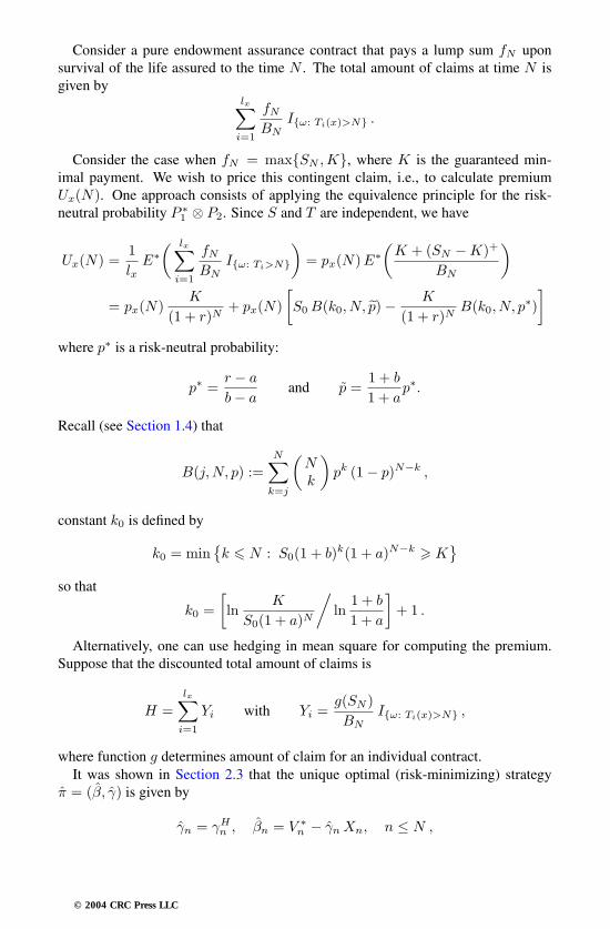
Consider a pure endowment assurance contract that pays a lump sum fN uponsurvival of the life assured to the time N . The total amount of claims at time N isgiven by

lx∑i=1

fNBN

Iω: Ti(x)>N .

Consider the case when fN = maxSN ,K, where K is the guaranteed min-imal payment. We wish to price this contingent claim, i.e., to calculate premiumUx(N). One approach consists of applying the equivalence principle for the risk-neutral probability P ∗

1 ⊗ P2. Since S and T are independent, we have

Ux(N) =1lx

E∗( lx∑i=1

fNBN

Iω: Ti>N

)= px(N)E∗

(K + (SN −K)+

BN

)= px(N)

K

(1 + r)N+ px(N)

[S0 B(k0, N, p)− K

(1 + r)NB(k0, N, p∗)

]where p∗ is a risk-neutral probability:

p∗ =r − a

b− aand p =

1 + b

1 + ap∗.

Recall (see Section 1.4) that

B(j,N, p) :=N∑k=j

(Nk

)pk (1− p)N −k ,

constant k0 is defined by

k0 = mink N : S0(1 + b)k(1 + a)N −k K

so that

k0 =[ln

K

S0(1 + a)N

/ln1 + b

1 + a

]+ 1 .

Alternatively, one can use hedging in mean square for computing the premium.Suppose that the discounted total amount of claims is

H =lx∑i=1

Yi with Yi =g(SN )BN

Iω: Ti(x)>N ,

where function g determines amount of claim for an individual contract.It was shown in Section 2.3 that the unique optimal (risk-minimizing) strategy

π = (β, γ) is given by

γn = γHn , βn = V ∗n − γnXn, n ≤ N ,


where Xn represents the capital of the portfolio, V πn represents the discounted capitalof the portfolio, and

V ∗n = E∗(H∣∣Fn) , n ≤ N ,

with respect to a risk-neutral probability P ∗. Sequence γH and martingale LH areuniquely determined by the Kunita-Watanabe decomposition (see Lemma 2.2).

Also we have the price-sequence

C πn = V πn −n∑k=1

γk∆Xk = E∗(H) + LHn ,

and the risk-sequence

Rπn = E∗((

LHN − LHn)2∣∣Fn).

Note that this strategy π = (β, γ) is not self-financing, but it is self-financing inaverage.

As an illustration we consider a lognormal model of a financial market:

Sn = S0 eh1+...+hn , hi = µ+ σ εn and Bn = B0 (1 + r)n ,

where εn are independent identically distributed normal random variables.

Let

g(SN ) = maxSN , K

= K + (SN −K)+ ,

where K is a constant.

Denote

h∗i = µ− δ + σ εn and S∗

k =SkBk

,

where δ = ln(1 + r). The discounting factor is ν = 1/(1 + r) and Nxt =∑lxk=1 Iω: Tk(x)≤t.


From properties of expectations we have

V πt =(lx −Nxt

)B−1

0 νN px+t(N − t)

×[K + St (1 + r)N−tΦ

(ln(St/K

)+ (N − t)

(δ + σ2/2

)σ√N − t

)

−K Φ

(ln(St/K

)+ (N − t)

(δ − σ2/2

)σ√N − t

)],

V π0 = lxB−10 νN px(N)

×[K + S0 (1 + r)N Φ

(ln(S0/K

)+N

(δ + σ2/2

)σ√N

)

−K Φ

(ln(S0/K

)+N

(δ − σ2/2

)σ√N

)].

Also

γHt =

(lx −Nxt

)B−1

0 νN px+t−1(N − t+ 1)S∗t−1

(expσ2 − 1)

×S∗t−1 B0 (1 + r)N

[Φ

(ln(St−1/K

)+ σ2 + (N − t+ 1)

(δ + σ2/2

)σ√N − t+ 1

)

−Φ(ln(St−1/K

)+ (N − t+ 1)

(δ + σ2/2

)σ√N − t+ 1

)]

+K

[Φ

(ln(St−1/K

)+ (N − t+ 1)

(δ − σ2/2

)σ√N − t+ 1

)

−Φ(ln(St−1/K

)+ σ2 + (N − t+ 1)

(δ − σ2/2

)σ√N − t+ 1

)],


andβHt = V πt − γHt S∗

t , t = 1, 2, . . . , N .

WORKED EXAMPLE 3.5A one-step model with lx = 2, N = 1.

SOLUTION The contingent claim is

H =maxS1, K Iω: T1>1

B1+maxS1, K Iω: T2>1

B1.

Let

B0 = 100, S0 = 100, K = 100, r = 0.01, µ = 5, σ = 0.5, px(1) = 0.999996,

thenδ ≈ 0.00995, ν =

100101

,

andV π0 ≈ 2.383, γH1 = 1.245.

Note that since φ(∞) = 1 and φ(−∞) = 0, we obtain

V π1 = (2−Nx1 )1B1

maxS1, K .

Here maxS1, K is the amount of an individual payment, (2 − Nx1 ) is thenumber of survivors, B1 is a discounting factor, and βH1 = V π1 − γH1 S∗

1 .Note that since sequence γH is predictable then value of γH1 is chosen at

time 0, i.e., when the value of S1 is unknown. The value of βH1 depends onS1 and therefore it is a random variable.

Now we consider a pure endowment assurance contract in the framework of acontinuous Black-Scholes model of a (B,S)-market.

Recall (see Section 2.6 for all details) that dynamics of asset S are described thefollowing stochastic differential equation

dSt = St(µdt+ σ dwt

),

and for a bank account B we have

dBt = r Bt dt , B0 = 1, t ≤ T .

As in the case of a binomial model, we assume that the Black-Scholes modelof a (B,S)-market is defined on a stochastic basis (Ω1,F1

T ,F1, P1), and randomvariables T1(x), T2(x), . . . Tlx(x) are defined on a stochastic basis (Ω2,F2

N ,F2, P2).


Then on the stochastic basis(Ω1 ⊗ Ω2,F1

N ⊗F2N ,F1 ⊗ F2, P1 ⊗ P2

),

we consider a pure endowment assurance contract with the discounted total amountof claims

lx∑k=1

maxST , KBT

Iω: Tk(x)>T .

To calculate premium Ux(T ), we compute the average of the latter sum with re-spect to probability P ∗ = P ∗

1 ⊗ P2:

Ux(T ) =1lx

E∗( lx∑k=1

maxST , KBT

Iω: Tk(x)>T

)(3.18)

= px(T )K e−rT + px(T )[S0 Φ

(d+(0)

)−K e−rT Φ(d−(0)

)],

where

d±(t) =ln(St/K

)+ (T − t)

(r ± σ2/2

)σ√T − t

,

and px(T ) is the probability that an individual of age x survives to age x+ T .This formula for premium Ux(T ) has the following obvious interpretation that is

based on the structure of the payment maxST , K = K + (ST −K)+. The firstterm px(T )K e−rT reflects the obligation to pay the guaranteed amount K. Clearly,K is discounted and multiplied by the survival function. The second term takesinto account both the risk of surviving and the market risk related to the payment ofamount (ST − K)+. The second risk component is estimated in terms of the priceof a European call option. Hence, the Black-Scholes formula is naturally used forcalculating Ux(T ).

REMARK 3.1

1. The discrete Gaussian model of a market gives the same results as hedg-ing in mean square in the Black-Scholes model if the discrete time t ≤ Nis replaced with the continuous time t ≤ T .

2. In practice, the premium sometimes is not paid as a lump sum at time0, but is arranged as a periodic payment. In this case, it is naturalto characterize the premium in terms of its density p(t), which can befound from the following equivalence relation:

Ux(T ) =∫ T

0

p(t) e−rt px(t) dt .


3. Recall that the contingent claim maxST , K can be perfectly hedgedin a complete market (see Section 2.1). The same hedge can be usedfor the mixed claim maxST , K Iω: Tk(x)>T , but it turns out thatpremium Ux(T ) is insufficient for perfect hedging since

Ux(T ) = px(T )E∗(maxST , K e−rT

)= x0 < E∗

(maxST , K e−rT

),

which can be interpreted as a budget constraint. Thus, one can usethe methodology of quantile hedging (see Section 2.6) to minimize riskrelated to such a contract.

The notion of reserve Vt is an important ingredient of actuarial mathematics. Thereserve at time t is defined as the difference between the value of future claims andthe value of future premiums:

Vt = px+t(T−t)E∗(maxST , K e−rt∣∣F1

t

)−∫ Tt

p(u) e−r(u−t) px+t(u−t) du .

Assuming that

px(t) = P2

(ω : Tk(x) > t) = exp−∫ t

0

µx+τ dτ

,

and using the Kolmogorov-Ito formula, we obtain the following equation for Vt ≡V (t, s):

∂V

∂t(t, s) = p(t)+

(µx+t+ r

)V (t, s)− 1

2σ2 s2 ∂2V

∂s2(t, s)− r s

∂V

∂s(t, s). (3.19)

Note that since V is a function of the price of asset S, then naturally the latter equa-tion is a generalization of the Black-Scholes equation. Otherwise, it reduces to thewell-known Thiele’s equation

∂V

∂t= p(t) +

(µx+t + r

)V .

On the other hand, if insurance characteristics p(t) = µx+t = 0, then equation (3.19)reduces to the Black-Scholes equation. Thus, we can summarize that equation (3.19)for the reserve reflects the presence of both insurance risk and financial risk.

3.5 Reinsurance risks

Reinsurance is a mechanism that insurance companies use to transfer some or allof their risks to reinsurance companies. The primary aim of reinsurance is to protect


the solvency of the insurance company by minimizing the probability of bankruptcy.Some typical examples of situations when such solvency protection is required in-clude receiving very large claims (e.g., in the cases of big man-made disasters suchas an aeroplane crash, etc.); receiving a large number of claims from policies af-fected by the same event (e.g., in the case of natural disasters such as earthquakes,hurricanes, floods, etc.); sudden changes in the premiums flow (say, due to inflation)or in the number of policy holders; the need to access some additional capital so thatthe insurance company can take on larger risks and therefore attract more clients.

As in Section 3.1 we consider a risk process

X(t) =N(t)∑i=1

Xi ,

which represents the aggregate amount of claims up to time t.One of the main characteristics of a reinsurance contract is quantity h(X) that

determines the amount of claims payment made by the insurance company. Theremainder X − h(X) is paid by the reinsurance company and is naturally referredto as an insured proportion of risk X . The insurance company pays premium to thereinsurance company in order to transfer this part of its risk.

Function h(X) is called the retention function. It has the following properties:

(a) h(X) and X − h(X) are non-decreasing functions;

(b) 0 ≤ h(X) ≤ X, h(0) = 0.

There are two basic forms of reinsurance: proportional reinsurance and non-proportional reinsurance. The main types of proportional reinsurance are quotashare and surplus. A quota share reinsurance transfers all risks in the same pro-portion, whereas in a surplus reinsurance proportions of transfer may vary. The typi-cal examples of non-proportional reinsurance are stop-loss reinsurance and excess ofloss reinsurance. They provide protection when claims exceed a certain agreed level.

The following retention functions

1. h(x) = a x 0 < a ≤ 1,

2. h(x) = mina, x a > 0,

correspond to the quota share reinsurance and the stop-loss reinsurance, respectively.From the point of view of the reinsurance company a reinsurance contract is just a

usual insurance against risk X − h(X). Hence one can calculate the correspondingpremium level using the methodology described earlier in this chapter:

Π = Π(X − h(X)

).

Let us consider a quota share reinsurance contract in the framework of the indi-vidual risk model. If Xi is the amount of an individual claim, then aXi is paid by


the insurance company and (1 − a)Xi by the reinsurance company. Thus the totalamount of claim

S = X1 + . . .+Xn

received by the insurance company is reduced to

aS = a (X1 + . . .+Xn) .

Suppose both insurance and reinsurance companies use the Expectation principlein the premium calculation (see Section 3.1), and the security loading coefficientsare θ and θ∗, respectively.

Prior to entering the reinsurance contract the capital of the insurance company is

x+ (1 + θ)E(S) .

After paying the premium (1 + θ∗) (1− a)E(S), the capital becomes

x+[θ − θ∗ + a (1 + θ∗)

]E(S) .

Now we compare the probabilities of insolvency as measures of risk to which theinsurance company is exposed when it purchases the reinsurance contract and whenit does not. In the first case it is

P(

ω : aS < x+[θ − θ∗ + a (1 + θ∗)

]E(S)

)

= P

(ω : S <

x+[θ − θ∗ + a (1 + θ∗)

]E(S)

a

),

and in the second:P(

ω : S < x+ (1 + θ)E(S))

.

This allows us to manage the risk of the insurance company, since if (θ−θ∗)E(S) <x, then the probability of bankruptcy can be reduced by purchasing the reinsurancecontract.

Next we consider a stop-loss reinsurance contract with the retention level a. Ac-cording to this contract, if the amount of an individual claim Xi ≤ a, then it is paidby the insurance company, otherwise the insurance company pays a and the rein-surance company pays the remainder Xi − a. So by purchasing such a reinsurancecontract the insurance company protects itself from paying more than a per individ-ual claim.

Suppose that the insurance company issues N identical insurance contracts, sothat the independent identically distributed random variables X1, . . . , XN representthe amounts of corresponding claims. Under the stop-loss reinsurance contract thetotal amount of claim

S = X1 + . . .+XN


received by the insurance company is reduced to

S(a) = X(a)1 + . . .+X(a)

n , where X(a) = minX, a .For example, the sequence of payments made by the insurance company may look

likeX1, X2, a, a, X5, . . . ,

and the corresponding sequence of payments made by the reinsurance company is

0, 0, X3 − a, X4 − a, 0, . . . .

Note that the number of claims paid by the reinsurance company may be less thanN . Nevertheless we can represent the risk process of the reinsurance company in theform

∑Ni=1 Zi, where some Zi may be equal to zero.

Again we assume that both insurance and reinsurance companies use the Expec-tation principle in the premium calculation, and that the security loading coefficientsare θ and θ∗, respectively.

The capital of the insurance company prior to entering the reinsurance contract isgiven by

N p = N (1 + θ) p0 ≡ N (1 + θ)E(X) .

After paying the premium

N (1 + θ∗)(E(X)− E(X(a))

),

it becomes

N (1 + θ)E(X) − N (1 + θ∗)(E(X)− E(X(a))

)= N (θ − θ∗)E(X) +N (1 + θ∗)E(X(a)) .

Hence the probability of insolvency is

P(

ω : S(a) > N (θ − θ∗)E(X) +N (1 + θ∗)E(X(a)))

.

It is rather difficult to compute this probability explicitly. We use the Central Limittheorem for computing its approximation:

P

(ω :

S(a) − E(S(a)

)√V(S(a)

) >N (θ − θ∗)E(X) +N θ∗ E(X(a))√

N V(X(a)

))

≈ 1− Φ(√

N(θ − θ∗)E(X) + θ∗ E(X(a))√

V(X(a)

)),

where

Φ(x) =1√2π

∫ x−∞

e−y2/2dy


is a standard normal distribution.Suppose that the insurance company can vary the retention level a (variation of a,

of course, changes the premium payable to the reinsurance company). Suppose thata is the maximum of function

ϕ(a) =

[(θ − θ∗)E(X) + θ∗ E

(minX, a)]2

V(minX, a) ,

then the stop-loss reinsurance contract with the retention level a minimizes the prob-ability of insolvency.

WORKED EXAMPLE 3.6Suppose that a random variable representing the amount of an individual claimis uniformly distributed in [0, x]. Consider a stop-loss reinsurance contract andfind the value of a that minimizes the probability of insolvency.

SOLUTION Clearly, we can assume that the retention level a < x. Thenwe have

E(X) =x

2, E

(X2)=

x2

3, V (X) =

x2

12,

and

E(X(a)

)= a− a2

2x, E

((X(a))2

)= a2 − 2a3

3x, V

(X(a)

)=

a3

3x− a4

4x2,

which implies

ϕ(a) =

[(θ − θ∗) x2 + θ∗

(a− a2

2x

)]2a3

3x − a4

4x2

.

Due to no-arbitrage considerations, we have that θ ≤ θ∗, since otherwisethe insurance company can transfer all the risk to the reinsurance companyand make a non-zero profit with zero initial capital. If we additionally assumethat θ∗ < 3 θ, then it is not difficult to see that function ϕ(a) has a uniquemaximum on [0, x]:

a =3x[θ∗ − θ

]2 θ∗

, so that ϕ(a) =(θ∗)2

99 θ − θ∗

θ∗ − θ.

There are large risks (e.g., a jumbo jet or an oil drilling platform) of a magnitudethat makes it impossible for most single insurance companies to insure the wholerisk without sharing this risk exposure. In this case, an insurer transfers some risk toa reinsurer. The reinsurer itself may also reinsure this risk, which is often referred toas retrocession. Thus, one can summarize that the insurance market has at least threelevels:


1. Primary market (insurance companies)

2. Reinsurance market (reinsurance companies)

3. Retrocession market (reinsurance companies that provide insurance to otherreinsurance companies)

Clearly, the retrocession market can consist of more than one level. For eachnth level reinsurance company, the risk transfer time, i.e., time between receiving arisk from a (n− 1)st-level company and passing it to a (n+1)st-level company, is arandom variable with some distribution F , and it is independent of risk transfer timesof another companies. Denote Σ

(Xn)

the total number of nth-level companies,and Rn,i the number nth-level companies that insured the ith company from (n −1)st level. We assume that Rn,i are independent random variables with distribution(pk)k=0,1,.... Note that

Xn = 1 , Xn+1 =Xn∑i=1

Rn,i .

Denote gXn(s) and gR(s) the generating functions of Xn and R, respectively.For |s| < 1 and all n ∈ N we have the following relation

gXn+1(s) = gXn

(gR(s)

)= gR

(gXn(s)

)= gR

(gR(. . . gR(s)

))︸︷︷︸

n times

,

which follows from the equality

gXn+1(s) ≡ E(sXn+1

)=

∞∑j=0

E

(s∑Xn

i=1 Rn,i

∣∣∣Xn = j

)P(ω : Xn = j)

= gXn

(gR(s)

),

applied n times.Using the latter formula and taking into account that

E(Xn+1) = E(Xn)E(R) and V (Xn+1) = V (Xn)(E(R)

)2 + E(Xn)V (R) ,

we obtainE(Xn) =

(E(R)

)2 ≡ µnR ,

and

V (Xn) =

µn−1

R (µnR−1)

µR−1 V (R) , µR = 1

nV (R) , µR = 1 .


Let Σ(X(t)

)be the number of companies involved in the contract up to time t,

and Xn,i(t) the number auxiliary companies that insured the ith company from nth

level after time t. It is clear that

X(t) =

1 , t < T∑Ri=1 X2,i(t− T ) , t ≥ T .

Let µ(t) = E(X(t)

), the average number of companies involved in a reinsurance

project at time t. The following results hold true.

PROPOSITION 3.1We have

µ(t) = F (t) + µR

∫ t0

µ(t− ν) dF (ν) , (3.20)

where F (x) is the distribution function of the risk transfer time, and F (x) =1− F (x).

PROOF Let random variable T represent the time between issuing theprimary insurance contract by a primary insurance company and the timewhen this risk is reinsured by a next level company. Then, using propertiesof conditional expectations, we obtain

µ(t) = E(E(X(t) |T )) = ∫ ∞

0

E(X(t) |T = ν

)dF (ν)

=∫ t

0

E(X(t) |T = ν

)dF (ν) +

∫ ∞

t

E(X(t) |T = ν

)dF (ν) .

Note that the conditional expectation in the second integral in the right-handside is equal to 1. To compute first term we write

E(X(t) |T = ν

)=

∞∑j=0

pj E(X(t) |T = ν , R = j

),

where R is the number of reinsurers of the primary company. Each second-level reinsurance company generates an independent chain of reinsurers.Hence

E(X(t) |T = ν , R = j

)= E

( j∑i=1

X2,i(t− ν) |T = ν , R = j)

= j µ(t− ν) ,

which implies the result.


The following result is typical for the theory of branching processes (see, for ex-ample, [40]).

PROPOSITION 3.2If distribution F is continuous then the following statements hold true.

1. If µR = 1, then µ(t) = 1 for all t ≥ 0.

2. If µR > 1, then

limt→∞

µ(t)eγt

=µR − 1

γ µ2R |l′T (γ)|

,

where γ is the unique solution of equation

lT (y) :=∫ ∞

0

e−x y dF (x) = µ−1R .

3. If µR < 1 and there exists a positive solution γ of equation

mT (y) :=∫ ∞

0

ey x dF (x) = µ−1R ,

then

limt→∞

µ(t)e−γt

=1− µR

γ µ2R |m′

T (γ)|,

otherwise this limit is equal to zero.

PROOF We prove here only the first statement. If µR = 1, then µ(t) ≡ 1is a solution of equation (3.20). Thus, we need only to establish the uniquenessof this solution to

µ(t) = F (t) +∫ t

0

µ(t− ν) dF (ν) ,

Suppose that both µ1(t) and µ2(t) are solutions of this equation. Then

µ1(t)− µ2(t) =∫ t

0

(µ1(t− ν)− µ2(t− ν)

)dF (ν)

if and only ifµ1(t)− µ2(t) =

(µ1 − µ2

) ∗ F (t) .Further

|µ1(t)− µ2(t)| = |(µ1 − µ2

) ∗ F (t)| = |(µ1 − µ2

) ∗ F ∗ F (t)|= . . .

= |(µ1 − µ2

) ∗ F ∗n(t)| ≤ F ∗n(t) supν∈[0,t]

|µ1(ν)− µ2(ν)| .


Now, since F ∗n(t) ≤ [F (t)]n, thenlimn→∞F ∗n(t) = 0 ,


WORKED EXAMPLE 3.7Describe the asymptotic behavior of µ(t) if the risk transfer time has an ex-ponential distribution.

SOLUTION We have

lT (y) :=∫ ∞

0

e−x y dF (x) =∫ ∞

0

e−x y λ e−λx dx =λ

λ+ y

andmT (y) :=

∫ ∞

0

ey x dF (x) =∫ ∞

0

ey x λ e−λx dx =λ

λ− y,

so that their derivatives are

l′T (y) = − λ

(λ+ y)2and m′

T (y) = − λ

(λ− y)2.

Sinceγ = λ (µR − 1) is a solution to lT (y) =

1µR

,

andγ = λ (1− µR) is a solution to mT (y) =

1µR

,

then we deduce that

1) if µR = 1, then µ(t) = 1 for all t ≥ 0;

2) if µR > 1, then

limt→∞

µ(t)eλ (µR−1) t

= 1 (exponential growth);

3) if µR < 1, then

limt→∞

µ(t)eλ (µR−1) t

= 1 (exponential decay).

In this case we can also find an exact expression for µ(t). Substitute F (y) =1− e−λy into equation (3.20):

µ(t) = e−λt + µR

∫ t0

µ(t− ν)λ e−λν dν .


Differentiating in t and integrating by parts, we obtain

µ′(t) = −λ e−λt + µR µ(0)λ e−λt − µR

∫ t0

λ e−λν dµ(t− ν)

= −λ e−λt + µR λµ(t)− λµR

∫ t0

µ(t− ν)λ e−λν dν

= µ(t)λ (µR − 1) .

The Cauchy problem

µ′(t) = µ(t)λ (µR − 1) , t ≥ 0 , µ(0) = 1 ,

has the unique solutionµ(t) = eλ (µR−1) t ,

which implies the asymptotic behavior as described above.

The structure of the traditional insurance market provides reasonable protectionto insurance companies against ‘moderately’ large risks. There are events (catastro-phes) that can give rise to giant claims, when the total claim amount can be compa-rable with the total premium income. For example, Hurricane Andrew (1992, USA)gave rise to the total claim equivalent to 1/5 of the combined total premium incomeof the insurance market of the USA. Floods in Europe in 2002 caused a situationwhere insurance companies had to rely on the financial intervention of governmentsand other organizations in order to stay solvent. Furthermore, some catastrophes maycause insured losses that are comparable to the capacity of the whole of the insur-ance industry. For instance, computer simulations of some earthquakes in Californiasuggest that they could cause losses up to $US 100 billion, whereas in the mid 1990sthe combined capital of the insurance industry was less than $US 300 billion.

Risk securitization is one of the possible ways of dealing with this situation. Itconsists of introducing insurance securities: catastrophe (CAT) bonds, forwards, fu-tures, options etc., as derivative instruments in catastrophe reinsurance. This form ofreinsurance is viable due to the 1:100 ratio of insurance industry to finance industry.

The first step in the process of risk securitization is related to choosing an under-lying asset that can be used to construct the corresponding CAT derivative securities.At the beginning of the 1990s it was the ISO-index (introduced by the InsuranceServices Office statistical agency, USA) that reflected the losses of a pool of mostsignificant insurance companies of the USA. From the mid 1990s the PCS-index(introduced by a non-profit organization Property Claim Service, USA) is the mostcommonly used. The PCS-index is based on actual losses from a catastrophic eventover some period of time. During the initial risk-period one assesses the catastrophicevent. This is followed by the period of losses development when the initial informa-tion is refined. At the beginning of the risk-period the PCS-index is set to be zero.Each point of it corresponds to US$ 100 million. The total amount of claim pay-ments is restricted to US$ 50 billion. Thus, we have the following expression for a


PCS-index L at time t:

Lt =XtC

,

where Xt is the loss process and C = US$ 100 million. Then, given a specificstructure of the loss process Xt, one can price CAT derivative securities using thepricing methods of financial risk management.

3.6 Extended analysis of insurance risks in a generalizedCramer-Lundberg model

As we discussed earlier, solvency of an insurance company is a natural character-ization of its exposure to risk, and the traditional actuarial measure of such exposurein the probability of insolvency (or bankruptcy).

Representing the capital R of the insurance company as the difference between thepremium process Π and risk process X , we can define the probability of solvency onfinite and infinite intervals as

ϕ(t, x) = P(ω : R(s) > 0 for all s ≤ t) , R(0) = x ,

ϕ(x) = P(ω : R(t) > 0 for all t ≥ 0) , R(0) = x ,

respectively.Suppose that

E(Π(t)

)> E

(X(t)

),

i.e., pure income is positive.This section is devoted to generalizations of the Cramer-Lundberg model. In par-

ticular, we study the probability of insolvency as a measure of exposure to risk insituations when the premium process Π has more complex structure than in the orig-inal model. We also will take into account various factors of financial and insurancemarkets.

First we consider a case when premiums are received at some random times andtheir amounts are also random. The capital of the company has the form

R(t) = x+N1(t)∑i=1

ci −N(t)∑i=1

Xi ,

where N1 and N are independent Poisson processes with intensities λ1 and λ, re-spectively, and (ci) and (Xi) sequences of independent random variables with dis-tribution functions G(·) and F (·), respectively.


Hence

λ1 t E(ci) = E

(N1(t)∑i=1

ci

)= E

(Π(t)

)> E

(X(t)

)

= E

(N(t)∑i=1

Xi

)= λ tE(Xi) .

Therefore the condition of positivity of pure income is reduced to inequality

λ1 E(ci) > λE(Xi) .

Under these assumptions we have that the probability of solvency satisfies theinequality

ϕ(x) ≥ 1− e−Rx ,

where constant R is a solution of the characteristic equation

λ1

[E(e−Rci

)− 1]+ λ[E(e−RXi

)− 1] = 0 .For exponential distribution functions G(·) (premium process) and F (·) (risk pro-

cess) we have the following result.

PROPOSITION 3.3If

G(x) = P(ω : ci ≤ x) = 1− e−b x ,

F (x) = P(ω : Xi ≤ x) = 1− e−a x ,

a > 0, b > 0, x > 0 ,

then we have an exact expression

ϕ(x) = 1− (a+ b)λ(λ1 + λ) a

expλ b− λ1 a

λ1 + λx

.

PROOF Using the independence of Π(t) and X(t), we have

E(e−R

[Π(t)−X(t)

])

=

( ∞∑k=0

e−λ1t(λ1 t)k

k!E(e−R

∑ki=1 ci

)) ( ∞∑k=0

e−λt(λ t)k

k!E(eR

∑ki=1Xi

))

= expλ1 t

[E(e−Rci

)− 1]+ λ t[E(eRXi

)− 1] ,


for any constant R. Now let R be a solution of the characteristic equation,then for t > s we have

E(e−R

[Π(t)−X(t)

]∣∣∣Fs)= e−R

[Π(s)−X(s)

]E(e−R

[Π(t)−Π(s)−X(t)+X(s)

]∣∣∣Fs)= e−R

[Π(s)−X(s)

]E(e−R

[Π(t−s)−X(t−s)

])= e−R

[Π(s)−X(s)

],

where Ft is a σ-algebra generated by processes Π(s) and X(s) up to time t.Hence the process

YR(t) = e−R[Π(t)−X(t)

]is a martingale with the initial condition YR(0) = 1.Consider the bankruptcy moment

τ = inft ≥ 0 : R(t) < 0 .Since the average value of a martingale is constant, we obtain

1 = E(YR(τ ∧ t)

) ≥ E(YR(τ ∧ t) Iω: τ≤t

)= E

(e−R

[Π(τ)−X(τ)

]Iω: τ≤t

)> eRx P

(ω : τ ≤ t) ,where we also used the fact that Π(τ)−X(τ) for τ < ∞. Passing to the limitas t → ∞, we obtain

ϕ(x) ≥ 1− e−Rx .

Note that if distribution functions G(·) and F (·) are exponential, then thecondition of positivity of pure income has the form

λ1

b>

λ

a,

and the characteristic equation is

λ1

[b

b+R− 1]+ λ

[a

a−R− 1]= 0 .

Hence constant R is either equal to zero or to

λ1 a− λ b

λ1 + λ.

Thus, we have that either ϕ(∞) = 1 or

ϕ(x) > 1− expλ b− λ1 a

λ1 + λx

.


As in Section 3.2 one can use the formula for total probability to obtain thefollowing integral equation for ϕ(x):

(λ+ λ1)ϕ(x) = λ1

∫ ∞

0

ϕ(x+ v) b e−bv dv + λ

∫ x0

ϕ(x− u) a e−au du .

Changing variables v1 = v + x, u1 = x− u, we can write ϕ(x) in the form

ϕ(x) =λ1

λ+ λ1

∫ ∞

x

ϕ(v1) b e−b(v1−x) dv1 +λ

λ+ λ1

∫ x0

ϕ(u1) a e−a(x−u1) du1 ,

which, in particular, indicates that function ϕ is differentiable. Also note that(∫ ∞

0

ϕ(x+ v) b e−bv dv)′

x

= −b ϕ(x) + b

∫ ∞

0

ϕ(x+ v) b e−bv dv ,

(∫ x0

ϕ(x− u) a e−au du)′

x

= aϕ(x)− a

∫ x0


Differentiating the equation for ϕ(x), we have

(λ+ λ1)ϕ′(x) + (λ1 b− λa)ϕ(x)

= b λ1

∫ ∞

0

ϕ(x+ v) b e−bv dv − aλ

∫ x0


Differentiating second time, we obtain

(λ+ λ1)ϕ′′(x) + (λ1 b− λa)ϕ′(x) + (λ1 b2 + λa2)ϕ(x)

= b2 λ1

∫ ∞

0

ϕ(x+ v) b e−bv dv + a2 λ

∫ x0


This implies that

ϕ′′(x) =λ b− λ1 a

λ+ λ1ϕ′(x) .

This equation has a solution of the form

ϕ(x) = C1 + C2 expλ b− λ1 a

λ+ λ1x

.

It is clear from the statement of the problem that

C1 = ϕ(∞) = 1 .

Substituting this expression into the initial integral equation for ϕ(x), weobtain that for x = 0

(λ+ λ1)ϕ(0) = λ1

∫ ∞

0

ϕ(v) b e−bv dv ,


and hence

C2 = − (a+ b)λ(λ+ λ1) a

,

which completes the proof.

REMARK 3.2 Similar results can be obtained for a discrete version ofthe Cramer-Lundberg model, when Π(t) and X(t) are independent compoundbinomial processes.

Now we consider a generalization of the Cramer-Lundberg model that takes intoaccount the insurance market competition. Suppose the pool of insurance compa-nies is large enough, and each company has only limited influence on the insurancemarket. Then it is natural to use Gaussian diffusion for modelling the capital of aninsurance company:

R(t) = x+Π(t)−X(t) + σ wt ,

where

Π(t) = µ t+N1(t)∑i=1

ci , µ > 0 ,

is the premium process,

X(t) =N(t)∑i=1

Xi ,

is the risk process, wt is a standard Wiener process and σ ≥ 0.It is assumed that all processes Π(t), X(t) and wt are independent and the condi-

tion of positivity of income:

µ+ λ1 E(ci) > λE(Xi) ,

holds true.In this case the probability of solvency again satisfies the estimate

ϕ(x) ≥ 1− e−Rx ,

where R is a solution of the characteristic equation

−Rµ+ σ2 R2 + λ1

[ ∫ ∞

0

e−Rv dG(v)− 1]+ λ

[ ∫ ∞

0

eRy dF (y)− 1]= 0 .

Another generalization of the Cramer-Lundberg model takes into account the factthat insurance companies are active participants of the financial market. Earlier wediscussed several discrete models of this type. Now we consider a version of Cramer-Lundberg model in the framework of a Black-Scholes market:

dBt = r Bt dt , B0 = 1 ,dSt = St

(µdt+ σ dwt

), S0 > 0 .


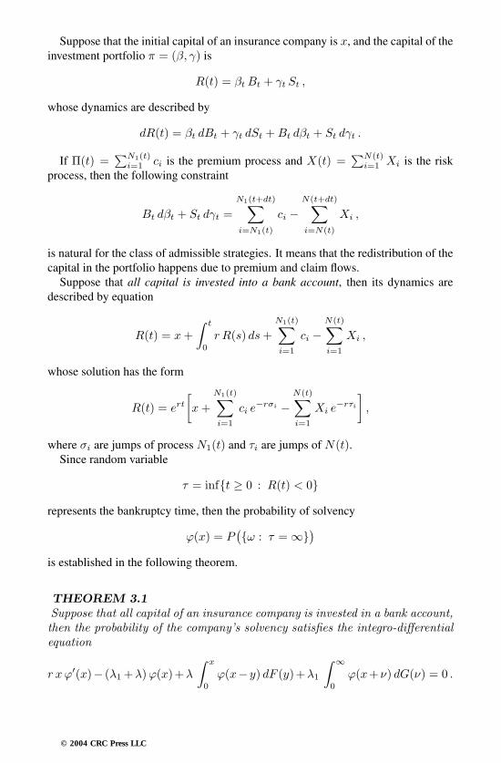
Suppose that the initial capital of an insurance company is x, and the capital of theinvestment portfolio π = (β, γ) is

R(t) = βtBt + γt St ,

whose dynamics are described by

dR(t) = βt dBt + γt dSt +Bt dβt + St dγt .

If Π(t) =∑N1(t)i=1 ci is the premium process and X(t) =

∑N(t)i=1 Xi is the risk

process, then the following constraint

Bt dβt + St dγt =N1(t+dt)∑i=N1(t)

ci −N(t+dt)∑i=N(t)

Xi ,

is natural for the class of admissible strategies. It means that the redistribution of thecapital in the portfolio happens due to premium and claim flows.

Suppose that all capital is invested into a bank account, then its dynamics aredescribed by equation

R(t) = x+∫ t

0

r R(s) ds+N1(t)∑i=1

ci −N(t)∑i=1

Xi ,

whose solution has the form

R(t) = ert[x+

N1(t)∑i=1

ci e−rσi −

N(t)∑i=1

Xi e−rτi

],

where σi are jumps of process N1(t) and τi are jumps of N(t).Since random variable

τ = inft ≥ 0 : R(t) < 0represents the bankruptcy time, then the probability of solvency

ϕ(x) = P(ω : τ =∞)

is established in the following theorem.

THEOREM 3.1Suppose that all capital of an insurance company is invested in a bank account,then the probability of the company’s solvency satisfies the integro-differentialequation

r xϕ′(x)− (λ1+λ)ϕ(x)+λ

∫ x0

ϕ(x− y) dF (y)+λ1

∫ ∞

0

ϕ(x+ν) dG(ν) = 0 .


PROOF Since for a fixed R(t) = x the further evolution of the processdepends neither on t nor on its history, then using the equation for R(t) wecan write for a small time interval ∆t:

ϕ(x) =[1− (λ1 + λ)

]ϕ(x+ r x∆t) + λ1

∫ ∞

0

ϕ(x+ r x∆t+ ν) dG(ν)

+λ∫ x

0

ϕ(x+ r∆t− u) dF (u) + o(∆t) .

Since by Taylor’s formula we have

ϕ(x+ r x∆t) = ϕ(x) + r∆t ϕ′(x) + o(∆t) ,

then dividing the latter equality by ∆t and taking limits as ∆ → ∞ provesthe claim.

To estimate the probability of solvency on a finite time interval we consider thediscounted capital R(t) = R(t) e−rt.

Clearly, for any finite interval we have

P(ω : R(s) ≥ 0 for all 0 ≤ s ≤ t)

= P(ω : R(s) ≥ 0 for all 0 ≤ s ≤ t) = ϕ(x, t) ,

since processes R(t) and R(t) are positive multiples of each other.Then we have the following estimate from below.

THEOREM 3.2For all R such that

f(R, t)

= exp∫ t

0

[λ1 + λ− λ1 E

(exp−Rci e

−rs)− λE(expRXi e

−rs)] ds< ∞

and for all t ≥ 0, the process e−RR(t)/f(R, t) is a martingale and

ϕ(x, t) ≥ 1− f(R, t) e−Rx .

PROOF Denote g(R(t), t) = e−RR(t), and compute

E(g(x, t+∆t)

)=[1− (λ1 + λ)∆t

]E(g(x, t)

)+λ1∆t

∫ ∞

0

g(x+ ν e−rt, t) dG(ν)

+λ∆t

∫ ∞

0

g(x− u e−rt, t) dF (u) + o(∆t) .


Hence we obtain the following integro-differential equation

∂

∂tE(g(x, t)

)+ (λ1 + λ) g(x, t)

= λ1

∫ ∞

0

g(x+ ν e−rt, t) dG(ν) + λ

∫ ∞

0

g(x− u e−rt, t) dF (u) .

Let us find a solution of the form E(g(x, t)

)= b(t) e−Rx. We obtain that b(t)

satisfies the equation

b′(t) = b(t)[− λ1 − λ+ λ1 E

(exp−Rci e

−rt)+ λE(expRXi e

−rt)]with the initial condition b(0) = 1.Further

E

(e−RR(t)

f(R, t)

∣∣∣∣Fs) = e−RR(s)

f(R, s)E(e−R(R(t)−R(s))

∣∣∣Fs) f(R, s)f(R, t)

=e−RR(s)

f(R, s)E(e−R(R(t)−R(s))

) f(R, s)f(R, t)

,

where the latter equality holds true due to the independence of increments ofR(t). Also note that random variables R(t)− R(s) and R(t− s) e−rs have thesame distribution function. Hence

E(e−R(R(t)−R(s))

)= E

(e−rsR(t−s)

)= e−(λ1+λ) (t−s) exp

∫ t−s0

[λ1 E

(exp−Rci e

−r(s+l))+λE

(expRXi e

−r(s+l))] dl

= e−(λ1+λ) (t−s) exp∫ t

s

[λ1 E

(exp−Rci e

−rl)+λE

(expRXi e

−rl)] dl=

f(R, t)f(R, s)

,

and therefore the process e−RR(t)/f(R, t) is a martingale.

Using martingale properties we obtain

1 =E(e−RR(t)

)f(R, t)

=E(e−RR(t∧τ))

f(R, t ∧ τ)≥ E

(e−RR(t∧τ) Iω: τ≤t

)f(R, t ∧ τ)

≥ eRx P(ω : τ ≤ t)f(R, t)

,


which proves the result.

Now suppose that all capital of an insurance company is invested in stock. Thedynamics of prices of stock S are described by the Black-Scholes model (with β0 =0). In this case the capital of the insurance company satisfies the equation

R(t) = µ

∫ t0

R(s) ds+ σ

∫ t0

R(s) dws +N1(t)∑i=1

ci −N(t)∑i=1

Xi .

We have the following result.

THEOREM 3.3Suppose that all capital of an insurance company is invested in stock, then theprobability of company’s solvency satisfies the integro-differential equation

σ2

2x2 ϕ′′(x) + µxϕ′(x)− (λ1 + λ)ϕ(x) (3.21)

+λ∫ x

0

ϕ(x− y) dF (y) + λ1

∫ ∞

0

ϕ(x+ ν) dG(ν) = 0 ,

which in the case of

G(ν) = 1− e−bν and F (u)1− e−au ,

can be reduced to a third order ordinary differential equation. For µ > σ2/2we have the asymptotic behavior

ϕ(x) = K1 + x1−2µ/σ2 (K2 + o(1)

).

PROOF (see, for example, [17]) As in Theorem 3.1 we can write

ϕ(x) =[1− (λ1 + λ)

]ϕ(x+ µx∆t+ σ x∆t)

+λ1

∫ ∞

0

ϕ(x+ µx∆t+ σ x∆t+ ν) dG(ν)

+λ∫ x+µx∆t+σ x∆t

0

ϕ(x+ µx∆t+ σ x∆t− u) dF (u) + o(∆t) .

Using the Kolmogorov-Ito formula we obtain

ϕ(x) =[1− (λ1 + λ)∆t

] (ϕ(x) + µxϕ′(x)∆t+

σ2

2x2 ϕ′′(x)∆t

)+λ1∆t

∫ ∞

0

ϕ(x+ ν) dG(ν) + λ∆t

∫ x0

ϕ(x− u) dF (u) ,


which implies (3.21).Now consider the case of

G(ν) = 1− e−bν and F (u) = 1− e−au .

Equation (3.21) becomes

(λ1 + λ)ϕ(x)− µxϕ′(x)− σ2

2x2 ϕ′′(x) = λ1 I1 + λ I , (3.22)

where

I1 =∫ ∞

0

ϕ(x+ ν) b e−bν dν and I =∫ x

0


SinceI ′1 = −b ϕ(x) + b I1 and I ′ = aϕ(x)− a I ,

then differentiating (3.22) we obtain

(λ1 + λ)ϕ′(x)− µϕ′(x) − µxϕ′′(x)− σ2 xϕ′′(x)− σ2

2x2 ϕ(3)(x)

= aλϕ(x)− aλ I − b λ1 ϕ(x) + b λ1 I1

or

(λ1 + λ− µ)ϕ′(x) − (µ+ σ2)xϕ′′(x)− σ2

2x2 ϕ(3)(x) (3.23)

= (aλ− b λ1)ϕ(x)− aλ I + b λ1 I1 .

Further differentiation gives

(λ1 + λ − µ)ϕ′′(x)− (µ+ σ2)ϕ′′(x)

−(µ+ σ2)xϕ(3)(x)− σ2 xϕ(3)(x)− σ2

2x2 ϕ(4)(x)

= (aλ− b λ1)ϕ′(x)− (b λ21 + aλ2)ϕ(x) + a2 λ I + b2 λ1 I1

or

(λ1 + λ− 2µ − σ2)ϕ′′(x)− (µ+ 2σ2)xϕ(3)(x)− σ2

2x2 ϕ(4)(x) (3.24)

= (aλ− b λ1)ϕ′(x)− (b λ21 + aλ2)ϕ(x) + a2 λ I + b2 λ1 I1 .


Now we multiply equation (3.22) by (a − b), equation (3.23) by a b, and addboth to equation (3.24):

ϕ(4)(x) +[(a− b) +

2 (µ+ 2σ2)σ2 x

]ϕ(3)(x)

+[− a b+

2 (µ+ σ2)(a− b)σ2 x

− 2 (λ1 + λ− 2µ− σ2)σ2 x2

]ϕ′′(x)

+[− 2 a b µ

σ2 x− 2

(λ1 a− λ b+ µ (b− a)

)σ2 x2

]ϕ′(x) = 0 .

Making substitution G = ϕ′, we obtain

G(3)(x) +[(a− b) +

2 (µ+ 2σ2)σ2 x

]G(2)(x)

+[− a b+

2 (µ+ σ2)(a− b)σ2 x

− 2 (λ1 + λ− 2µ− σ2)σ2 x2

]G′(x)

+[− 2 a b µ

σ2 x− 2

(λ1 a− λ b+ µ (b− a)

)σ2 x2

]G(x) = 0 .

We can use standard methods of theory of ordinary differential equations(see, for example, [20]) to find the asymptotic behavior of a solution of thelatter equation as x → ∞. We use the substitution G(x) = eτxG1(x) whereτ is chosen so that the constant coefficient in front of G1(x) vanishes. Thisimplies that τ satisfies the equation

τ3 + τ2 (a− b)− τ a b = 0 ,

which has solutions τ = 0, −a, b. The case of τ = b is not suitable as ϕ(x)is a bounded function. If τ = 0, then the equation stays unchanged. Next,we use the substitution G1(x) = xr G2(x) with r such that the coefficient infront of G2(x)/x is zero. Hence r satisfies the equation

−r a b− 2 a b µσ2

= 0 ,

which implies r = −2µ/σ2.Thus, we find a solution in the form of the series

G2(x) =∞∑k=0

ckxk

,

which, in general, may be divergent, but it gives us the following asymptoticrepresentation

G2(x) = c0 + o(1) .


In this caseϕ′(x) = x−2µ/σ2 (

c0 + o(1)).

If τ = −a, thenϕ′(x) = o

(x−2µ/σ2)

.

Note that this theorem reiterates the following important observation: if an in-surance company has investments in risky assets of the financial market, then theasymptotic behavior of the probability of its solvency cannot be exponential as itwas in the standard Cramer-Lundberg model.


App endix A

Software Supplement: Computationsin Finance and Insurance

The software is offered in the form of an open source code. It can be downloadedfrom

www.crcpress.com/e products/downloads/download.asp?cat no = C429

Any C++ compiler can be used under a Linux or Windows operating system. Thiscode can be easily read and modified.

Software berprog.cpp: Forecast of stock prices in aBernoulli market

Suppose that price dynamics of stock S in a Bernoulli market are given by thefollowing recurrence formula

Si+1 = Si (1 + ρ) , 0 ≤ i ≤ n ,

where ρ is the profitability of S and it takes values b or a with probabilities p and(1 − p), respectively. Assuming that the initial price is S0, we forecast the averageprice of S at time n.

The inputs are:

1. S0, the initial price of S;

2. a and b, values of possible change (as a percentage) in price of S;

3. p, the probability for ρ to take value b;

4. n, time horizon.

The forecast is based on the properties of conditional expectations E(Y |X) ofindependent random variables. Namely, we compute

Sav = E

(S1 + S2 + · · · + Sn

n

∣∣∣∣S0

).


http://www.crcpress.com/e_products/downloads/download.asp?cat_no=C429

In a two-step case we have

Sav = E

(S1 + S2

2

∣∣∣∣S0

)= E

(S0 (1 + ρ1 ) + S0 (1 + ρ1)(1 + ρ2)

2

∣∣∣∣S0

)

=S0

2

[E (1 + ρ1 ) + E (1 + ρ1 )E(1 + ρ2)

]=S0

2

[(1 + a)p + (1 + b)(1 − p)

+((1 + a)p + (1 + b)(1 − p)

) ((1 + a)p+ (1 + b)(1 − p)

)]=S0

2

[(1 + a)p + (1 + b)(1 − p) +

((1 + a)p + (1 + b)(1 − p)

)2]

Software binoptprice.cpp:Pricing options in a binomialmarket

Consider a one-step binomial (B,S )-market. Dynamics of a bank account andstock price are given by

B1 = B0 (1 + r ) , and S1 = S0 (1 + ρ) ,

where r is a fixed rate of interest and ρ is the profitability of S that takes values b ora with probabilities p and (1 − p), respectively. Quantities a, b r must satisfy theinequality −1 < a < r < b. Suppose that B0 = 1. Consider a European call optionwith the contingent claim

f1 = (S1 −K)+ = max(0, S1 −K) ,

where K is a strike price. Let K = S0. The intuitive price for this option is

E

(f1

1 + r

)=p (S0 b)+ + (1 − p) (S0 a)+

1 + r.

Alternatively, using the minimal hedging approach (see Section 1.4), one can con-struct a strategy π0(b0, g0 ) such that

Xπ1

(Xπ

0

) = f1 .

In this caseXπ

0 = β∗0 B0 + γ∗0 S0 ,


where

γ∗0 =f

(1)1 − f

(2)1

S0(ρ1 − ρ2), and β∗

0 =1

(1 + r)B0

(f

(1)1 − γ∗0S0(1 + ρ1)

).

Finally, consider a risk-neutral probability E∗ such that

E∗(S1

B1

)= S0.

This implies

p∗ =(1 + r)B0 − 1 − a

b− a.

If B0 = 1 then

p∗ =r − a

b− a.

Thus, risk-neutral price is given by

C = E∗(

f11 + r

)=f

(1)1 p∗ + f

(2)1 (1 − p∗)

1 + r.

The inputs are



3. p, the probability for ρ to take value b;

4. r, the rate of interest.

The outputs are

1. values of the contingent claim;

2. intuitive price;

3. initial capital of the minimal hedge;

4. risk-neutral price;

5. risk-neutral probability.


Software CRRoptprice.cpp: Call-put parity in a Cox-Ross-Rubinstein market

Now we consider a N -step binomial (B,S )-market. The Cox-Ross-Rubinsteinformula

CN = S0B(k0, N, p) −K (1 + r)−NB(k0, N, p∗)

gives the risk-neutral price of a European call option. Here p∗ is a risk-neutral prob-ability:

p∗ =r − a

b− aand p =

1 + b

1 + ap∗.

Recall (see Section 1.4) that

B (j,N, p) :=N∑

k=j

(Nk

)pk (1 − p)N−k ,

constant k0 is defined by

k0 = mink N : S0(1 + b)k(1 + a)N−k K

so that

k0 =[ln

K

S0(1 + a)N

/ln

1 + b

1 + a

]+ 1 .

Using the call-put parity, we can price a European put option with the claim

fN = (K − SN )+.

Namely, price of this option is given by

PN = CN − S0 +K(1 + r)−N .

The inputs are


2. K, the strike price;


4. r, the rate of interest;

5. N , the terminal time.

The output contains prices of the European call and put options.


Software amoptprice.cpp: Pricing an American call op-tion

Consider an N -step binomial (B,S)-market. Recall (see Section 1.5) that priceof an American call option with the sequence of claims

fn = (Sn −K)+ , n ≤ N ,

is defined by

CamN = sup

τ∈MN0

C(fτ ) = supτ∈MN

0

E∗(

fτ

(1 + r)τ

).

Computing

Yn = max

fn

(1 + r)n, E∗(Yn+1

∣∣Fn

)we obtain

CamN = Y0 .

The inputs are






The output consists of a price of the American call option.

Software spread.cpp: Computing spreads in a marketwith constraints

Let (B1, B2, S) be a Cox-Ross-Rubinstein market with constraints (see Section2.2). We find the interval [C∗, C∗] of all arbitrage-free prices, and therefore computespread C∗ − C∗ as a measure of incompleteness of the market.

The inputs are





4. r1 and r2, the rates of interest on saving and credit accounts, respectively;


The output contains prices of the European call option corresponding to given ratesr1 and r2, and the spread of the market.

Software BandSgreek.cpp: Pricing contingent claims us-ing the Black-Scholes formula and computing Greek pa-rameters in the continuous case

In Section 2.6 we studied pricing of contingent claims in a Black-Scholes modelof a (B,S)-market. The ‘fair’ arbitrage-free price of a European call option is givenby the Black-Scholes formula:

CT = S0 Φ(y+

)−K e−r T Φ(y−

),

where

y± =ln(S0/K) + T (r ± σ2/2)

σ√T

.

The price of a European put option:

PT (K,σ, S0) = CT (−K,−σ,−S0)

is derived from the call-put parity relation.The following ‘Greeks’ are used by the risk management practitioners:

Theta:

θ =∂CT

∂t=St σ ϕ

(y+(t)

)2√T − t

−K r e−r (T−t) Φ(y−(t)

),

Delta:

∆ =∂CT

∂S= Φ

(y+(t)

),

Rho:

ρ =∂CT

∂r= K (T − t) e−r (T−t) Φ

(y−(t)

),

Vega:

Υ =∂CT

∂σ= St ϕ

(y+(t)

)√T − t ,

The inputs are




3. σ, the volatility of the market;


5. T , the terminal time;

6. t, intermediate time.

The output contains prices of the European call and put options and values of‘Greek’ parameters.

Software BandSdiv.cpp: Pricing contingent claims usingthe Black-Scholes formula in a model with dividends

In the case when a holder of asset S receives dividends, the Black-Scholes formulagives the price of a European call option in the following form

CT (δ) = S0 e−δT Φ

(ln(S0/K) + T (r − δ + σ2/2)

σ√T

)

−K e−rT Φ(

ln(S0/K) + T (r − δ − σ2/2)σ√T

).

The inputs are



3. σ, the volatility of the market;


5. T , the terminal time;

6. δ, the dividends rate.

The output contains price of the European call option in the market with dividends.


Software Indicators.cpp: Some indicators used in techni-cal analysis

This software supplements Section 2.9. We compute the following indicators:

1. Simple Moving Average (SMA);

2. Weighted Moving Average (WMA);

3. Exponential Moving Average (EMA);

4. Bollinger Bands;

5. Moving Average Convergence/Divergence (MACD);

6. Relative Strength Index (RSI);

7. Parabolic Time Price system (PTP);

8. Volume Price Trend (VPT).

The user has to specify which indicator must be calculated. The software containstwo data files: ‘data.txt’ and ‘datav.txt’. File ‘data.txt’ contains close prices fromdaily bar charts for shares of Microsoft for the period from April, 2001 till April,2002. File ‘datav.txt’ contains the complete information of the same bar charts:daily open, close, low, high prices and trading volumes. First six indicators use file‘data.txt’, and the last two use file ‘datav.txt’. The resulting text file can be processedby various graphical tools, e.g. Gnuplot, MetaStock etc.

Simple Moving Average represents the average value of a quantity during a speci-fied period of time. At time j it is computed as

SMAj =1N

j∑i=j−N

vi ,

where vi, j−N ≤ i ≤ j, are values of this quantity. Input N defines the timehorizon. The output file ‘series’ contains the initial time series, and file ‘ma’contains the time series for moving average.

Weighted Moving Average is a modification of the SMA:

WMAj =N∑

i=1

&i vi ,


where &i are weights with∑N

i=1&i = 1. As above, time horizon N cor-responds to some analysis time j. Usually, time points that are closer to theanalysis time j, have heavier weights. We use the following formula

&i =i∑N

k=1 k, i = 1, . . . , N .

The output file ‘series’ contains the initial time series, and file ‘wma’ containsthe time series for weighted moving average.

Exponential Moving Average is the most widely used modification of the WMA.It uses all preceding values, but times that are distant from the analysis time j,correspond to very small weights. The Exponential Moving Average is definedby the formula

EMAj = (1 − α)EMAj−1 + α vj ,

where

α =2

N + 1.

Clearly, this is the simplest Moving Average indicator. File ‘ema’ contains thetime series for exponential moving average.

Bollinger Bands. First, one can use any of the Moving Average indicators to con-struct a Middle Band with values mj . Then Upper and Lower Bands are de-fined by

uj = mj + k σj and lj = mj − k σj ,

where

σj =

√∑ji=j−N (vi −mj)2

N.

The inputs include the order of averaging N and coefficient k which reflectsthe sensitivity of the indicator. The output file ‘bbands’ contains Middle, Up-per and Lower Bands.

Moving Average Convergence/Divergence is constructed in the following way:

1. compute short Moving Average;

2. compute long Moving Average;

3. compute quick line by subtracting long Moving Average from the shortMoving Average;

4. compute signal line by smoothing quick line with the help of MovingAverage;

5. compute MACD as the difference between signal and quick lines – thisis contained in the output file ‘macd’.


Relative Strength Index is computed in terms of average increase and decrease ofprice over some period of time.

Average increase is given by

Uj =

Uj−1(N−1)+(vj−vj−1)

N if vj > vj−1

Uj−1(N−1)N if vj < vj−1 .

Similarly, for average decrease we have

Dj =

Dj−1(N−1)+(vj−1−vj)

N if vj < vj−1

Dj−1(N−1)N if vj > vj−1 .

Then

RSIj = 100 − 1001 + Uj/Dj

.

The output file ‘rsi’ contains the values of RSI.

Parabolic Time Price system is represented by a line that is positioned either aboveor below the price graph, which identifies decreasing or increasing trends, re-spectively. The close price Cj is determined daily by the recurrence relation

Cj = Cj−1 + A (Ej−1 − Cj−1) ,

where E is the critical level of daily trading: in a long position it is equal to thehighest price since buying, in a short position it is the lowest price since selling.Constant A is the averaging factor. It determines how fast the close priceshould be shifted toward open position, and it depends on the number of newpeaks since buying and new lows since selling. The initial value of A is usuallyset to be 0.02. Increase or decrease of the initial value respectively increasesor decreases the sensitivity of PTP line. Note that in this computer versionof constructing PTP lines, by open position we understand the correspondingdynamics of a trend.

This software does not have any input parameters, but the input data in file‘datav.txt’ must be in the form (open, low, high, close).

Volume Price Trend reflects overbuying or overselling in the market. It is com-puted as

V PTj = V PTj−1 + VjPj − Pj−1

Pj−1,

where Vj and Pj are values of volume and price respectively.


Software elenshure.cpp: Pure endowment assurance

This software is the computer realization of Worked Example 1.5 from Section1.4.

The inputs are





5. N , the terminal time;

6. px, the probability of surviving.

The output is the price of the insurance policy.

Software var.cpp: Computing the Value at Risk

This software uses historical modelling and Monte-Carlo modelling for computingvalues of Value at Risk. Both approaches have similar structure, the only differenceis that in historical modelling one uses the real data for determining the distribu-tion of losses and profits, whereas, in Monte-Carlo modelling, it is assumed pricemovements are normally distributed.

The software computes the Value at Risk for one asset. File ‘vardata.txt’ containsthe input data. After assessing the volume of the input data, the software asks todefine the time horizon. Given this information it then determines the number ofpossible scenarios. Depending on the number of scenarios requested by the user,the software creates as many independent scenarios as possible and computes thedistribution of profits and losses. Further, it requests the value of probability forwhich we compute the Value at Risk, i.e., losses that correspond to this probabilitywill not exceed the corresponding value of the Value at Risk. Finally, since the inputdata is discrete in time, the software requests the size of the data confidence intervalin terms of probability of being in this interval and then calculates the confidenceinterval for the Value at Risk.


Software RiskPremInd.cpp: Computing premiums in themo del of individual risk

This software is the computer realization of Example from Section 3.1. It requeststhe level of bankruptcy’s probability and n, the number of policies. The initial datais contained in file ‘RPIdata.txt’ and it consists of uniformly distributed indepen-dent random variables that are used for computing the distribution of X ind, the totalpayoff to the policy holders. The output is the price of the insurance policy.


App endix B

Problems and Solutions

B.1 Problems for Chapter 1

Problem B.1.1 Suppose that the effective annual rate of interest is 10%. Find thepresent value of a 3-year bond with face value $500 and with annual coupon pay-ments of $100.

SOLUTION We have

B0 =100

1 + 0.1+

100(1 + 0.1)2

+100

(1 + 0.1)3+

500(1 + 0.1)3

≈ 624 ($) .

Problem B.1.2 An investor buys two European put options with strike price $40 andone European call option with strike price $50 on the same stock S with the sameexpiry date N . The total price of these options is $10. Write down the gain-lossfunction and discuss the possible outcomes.

SOLUTION If SN is the price of the asset at time N , then the gain-lossfunction has the form

V(SN ) = 2(40 − SN

)+ +(SN − 50

)+ − 10 .

We have the following cases.

(1) If SN < 40, then the put options are exercised and the call option is not.In this case

V(SN ) = 2(40 − SN

)+ − 10 = 70 − 2SN ,

and a profit is earned if SN < 35.

(2) If 40 ≤ SN ≤ 50, then none of the options are exercised, and the premiumis lost:

V(SN ) = −10 .


(3) If SN > 50, then only the call option is exercised:

V(SN ) =(SN − 50

)+ − 10 = SN − 60 ,

and a profit is earned if SN > 60.

Thus, this investment strategy reflects the investor’s expectation that theprice of S will be less than $35. Note that the maximal possible loss cannotbe higher than the amount of premium.

Problem B.1.3 The joint distribution of profitabilities α and β is given in the fol-lowing table.

α β −0.1 0 0.1

− 0.2 0.1 0 0.4

0.1 0.3 0.1 0.1

Find their individual distributions, average of β and the conditional expectationE(β|α).

SOLUTION From the given table we compute:

P(ω : α = −0.2) = 0.1 + 0.4 = 0.5

P(ω : α = 0.1) = 0.3 + 0.1 + 0.1 = 0.5

P(ω : β = −0.1) = 0.1 + 0.3 = 0.4

P(ω : β = 0) = 0.1

P(ω : β = 0.1) = 0.4 + 0.1 = 0.5 ,

which impliesE(β) = −0.1 × 0.4 + 0.1 × 0.5 = 0.01 .

The conditional expectation E(β|α) can be written in the form (see [41], forexample):

E(β|α) = E(β∣∣ω : α = −0.2) Iω: α=−0.2+E

(β∣∣ω : α = 0.1) Iω: α=0.1 .

Computing

E(β|ω : α = −0.2) = −0.1P

(ω : β = −0.1∣∣ω : α = −0.2)+0.1P

(ω : β = 0.1∣∣ω : α = −0.2)=

−0.1 × 0.1 + 0.1 × 0.40.5

= 0.06 ,


and

E(β|ω : α = 0.1) = −0.1P

(ω : β = −0.1∣∣ω : α = 0.1)+0.1P

(ω : β = 0.1∣∣ω : α = 0.1)=

−0.1 × 0.3 + 0.1 × 0.10.5

= −0.04 ,

we obtain E(β|α) = 0.06 Iω: α=−0.2 − 0.04 Iω: α=0.1 .

Note that

E(E(β|α)

)= 0.06 × 0.5 − 0.04 × 0.5 = 0.01 = E(β) .

Problem B.1.4 Suppose that analysis of the market data suggests that the price ofa certain asset S will increase by 2% in one month’s time with probability p, or willdecrease by 1% with probability 1−p. Find all values of p such that an investment inthis asset will be, on average, more profitable than an investment in a bank accountwith effective monthly interest rate of 1%.

SOLUTION The ave rage monthly profitability of an i nvestment in assetS is equal to

0.02 p− 0.01 (1 − p) = 0.03 p− 0.01 .

Hence p must satisfy0.03 p− 0.01 ≥ 0.01 ,

or p ≥ 2/3.

Problem B.1.5 As in Section 1.3 we consider a binomial (B,S)-market. Supposewe are given the following values of its parameters:

a = −0.4 , b = 0.6 , r = 0.2 , B0 = 1 , S0 = 200 .

Find the price and the minimal hedge of a ‘look back’ European call option withthe contingent claim

f2 =(S2 −K2

)+, where K2 = minS0, S1, S2 .

SOLUTION First we compute the risk-neutral probability

p∗ =r − a

b− r=

0.2 + 0.40.6 + 0.4

= 0.6 .


Now we write all possible prices of S and values of claim f2 in the followingtable.

event probability ρ1 ρ2 S0 S1 S2 K2 f2

ω1 0.16 −0.4 −0.4 200 120 72 72 0

ω2 0.24 −0.4 0.6 200 120 192 120 72

ω3 0.24 0.6 −0.4 200 320 192 192 0

ω4 0.36 0.6 0.6 200 320 512 200 312

We compute price of this claim:

C2 =E∗(f2)(1 + r)2

=0.16 × 0 + 0.24 × 72 + 0.24 × 0 + 0.36 × 312

1.44= 90 .

Next we find the minimal hedge π∗ =(βn, γn

)2n=1

that replicates claim f2.Consider time n = 1. Since the value of profitability ρ1 is known at this time,we can construct the pair

(β2, γ2

). Indeed, we have that hedge π∗ replicates

f2:Xπ∗

2 = f2 ,

which can be written in the form of the following systemXπ∗

2 (ω1) = β2(ω1) (1 + r)2 + γ2(ω1)S2(ω1)Xπ∗

2 (ω2) = β2(ω2) (1 + r)2 + γ2(ω2)S2(ω2)Xπ∗

2 (ω3) = β2(ω3) (1 + r)2 + γ2(ω3)S2(ω3)Xπ∗

2 (ω4) = β2(ω4) (1 + r)2 + γ2(ω4)S2(ω4) .

Substituting all known values we obtain0 = β2(ω1) (1 + 0.2)2 + γ2(ω1) 7272 = β2(ω2) (1 + 0.2)2 + γ2(ω2) 1920 = β2(ω3) (1 + 0.2)2 + γ2(ω3) 192312 = β2(ω4) (1 + 0.2)2 + γ2(ω4) 512 .

Since random variables β2 and γ2 do not depend on ρ2, we also have

β2(ω1) = β2(ω2) , β2(ω3) = β2(ω4) ,

andγ2(ω1) = γ2(ω2) , γ2(ω3) = γ2(ω4) .

Hence β2(ω1) = β2(ω2) = −30γ2(ω1) = γ2(ω2) = 0.6β2(ω3) = β2(ω4) = −130γ2(ω3) = γ2(ω4) = 39/40 .


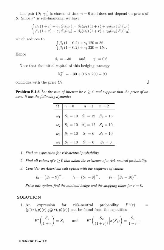
The pair(β1, γ1

)is chosen at time n = 0 and does not depend on prices of

S. Since π∗ is self-financing, we haveβ1 (1 + r) + γ1 S1(ω1) = β2(ω1) (1 + r) + γ2(ω1)S1(ω1)β1 (1 + r) + γ1 S1(ω3) = β2(ω3) (1 + r) + γ2(ω3)S1(ω3) ,

which reduces to β1 (1 + 0.2) + γ1 120 = 36β1 (1 + 0.2) + γ1 320 = 156 .

Henceβ1 = −30 and γ1 = 0.6 .

Note that the initial capital of this hedging strategy

Xπ∗0 = −30 + 0.6 × 200 = 90

coincides with the price C2.

Problem B.1.6 Let the rate of interest be r ≥ 0 and suppose that the price of anasset S has the following dynamics

Ω n = 0 n = 1 n = 2

ω1 S0 = 10 S1 = 12 S2 = 15

ω2 S0 = 10 S1 = 12 S2 = 10

ω3 S0 = 10 S1 = 6 S2 = 10

ω4 S0 = 10 S1 = 6 S2 = 3

1. Find an expression for risk-neutral probability.

2. Find all values of r ≥ 0 that admit the existence of a risk-neutral probability.

3. Consider an American call option with the sequence of claims

f0 =(S0 − 9

)+, f1 =

(S1 − 9

)+, f2 =

(S2 − 10

)+.

Price this option, find the minimal hedge and the stopping times for r = 0.

SOLUTION

1. An expression for risk-neutral probability P ∗(r) =(p∗1(r), p

∗2(r), p

∗3(r), p

∗4(r)

)can be found from the equalities

E∗(

S1

1 + r

)= S0 and E∗

(S2

(1 + r)2

∣∣∣σ(S1))

=S1

1 + r,


which reduce to the following system

12 (p∗1 + p∗2) + 6 (p∗3 + p∗4) = 10 (1 + r)

15 p∗1+10 p∗

2p∗1+p∗

2= 12 (1 + r)

10 p∗3+3 p∗

4p∗3+p∗

4= 6 (1 + r)

p∗1 + p∗2 + p∗3 + p∗4 = 1 .

Solving this system, we obtain

p∗1(r) =2 + 5 r

32 + 12 r

5, p∗2(r) =

2 + 5 r3

3 − 12 r5

,

p∗3(r) =1 − 5 r

33 + 6 r

7, p∗4(r) =

1 − 5 r3

4 − 6 r7

.

2. The fact that all these probabilities must be strictly positive:

p∗1(r) > 0 , p∗2(r) > 0 , p∗3(r) > 0 , p∗4(r) > 0 ,

implies that 0 ≤ r < 0.2.

3. Now since P ∗(0) =(4/15, 2/5, 1/7, 4/21

), we can compute all possible

values of our contingent claim:

event probability S0 f0 S1 f1 S2 f2

ω1 4/15 10 1 12 3 15 5

ω2 2/5 10 1 12 3 10 0

ω3 1/7 10 1 6 0 10 0

ω4 4/21 10 1 6 0 3 0

For pricing this option we compute

E∗(Y π∗2

∣∣ω : S1 = 12) = E∗(f2∣∣ω : S1 = 12) =5 p∗1 + 0 p∗2p∗1 + p∗2

= 2 ,

E∗(Y π∗2

∣∣ω : S1 = 6) = E∗(f2∣∣ω : S1 = 6) =0 p∗3 + 0 p∗4p∗3 + p∗4

= 0 ,

where Y π∗i is the capital of the minimal hedge π∗ at time i. Hence

Y π∗1 (ω1) = Y π∗

1 (ω2) = maxf1, E

∗(Y π∗2

∣∣ω : S1 = 12) = 3 ,

Y π∗1 (ω3) = Y π∗

1 (ω4) = maxf1, E

∗(Y π∗2

∣∣ω : S1 = 6) = 0 .


This implies

E∗(Y π∗1

∣∣F0

)= 3 (p∗1 + p∗2) + 0 (p∗3 + p∗4) = 3

(415

+25

)= 2 ,

and Y π∗

0 = maxf0, E

∗(Y π∗1

∣∣F0

)= 2 ,

therefore the price is C2 = 2.

To construct the minimal hedge π∗ we first compute the stopping times:

τ∗n = mini : n ≤ i ≤ 2 and Y π∗

i = fi

,

soτ∗ = τ∗1 = 1, τ∗2 = 2 .

Now due to equality Y π∗1 = f1, we have

Y π∗1 (ω) = β1 + γ1 S1(ω) = f1(ω)

or Y π∗

1 (ω1) = Y π∗1 (ω2) = β1 + γ1 12 = 3

Y π∗1 (ω3) = Y π∗

1 (ω4) = β1 + γ1 6 = 0 .

Hence β1 = −3 and γ1 = 0.5. Also note that the initial capital Y π∗0 =

−3 + 10 × 0.5 = 2 coincides with the price of the option.

Problem B.1.7 Consider a single-period binomial (B,S)-market with B0 = 1,S0 = 300, r = 0.1 and

S1 =


As in Section 1.6 use the logarithmic utility function to find an optimal strategy withthe initial capital 200.

SOLUTION First we compute parameters

a =250 − 300

300= −1

6and b =

350 − 300300

=16.

The average profitability of S with respect to the initial probability is

m =410

−16

+610

16

=130.


Then, according to formula (1.5), the proportion of risky capital in the re-quired strategy must be

α∗ =(1 + r) (m− r)(r − a) (b− r)

= −4.125 .

On the other hand,

α∗ = γ∗S∗

0

Xπ∗0

,

hence,

γ∗ = −4.125200300

= −2.75 .

The non-risky component β∗ can be found from the condition of self-financing:

Xπ∗0 = β∗ + γ∗ S0 ,

which impliesβ∗ = 200 + 2.75 × 300 = 1025 .

Problem B.1.8 Repeat Problem B.1.7 with B0 = 1, S0 = 100, r = 0.2 and

S1 =


SOLUTION In this case we have

a =80 − 100

100= −0.2 and b =

150 − 100100

= 0.5 .

Thenm = 0.7 × 0.5 − 0.3 × 0.2 = 0.29 ,

and

α∗ =(1 + r) (m− r)(r − a) (b− r)

= 0.9 .

Thus

γ∗ = α∗ Xπ∗0

S∗0

= 0.9200100

= 1.8 ,

andβ∗ = Xπ∗

0 − γ∗ S0 = 200 − 1.8 × 100 = 20 .



Problem B.2.1 Consider a single-period (B,S)-market with B0 = 1, S0 = 10,r = 0.2 and

S1(ω1) = 6, S1(ω2) = 12, S1(ω3) = 18 .

Find risk-neutral probability P ∗.

SOLUTION An expression for P ∗ can be found from the equality

E∗(

S1

1 + r

)= S0 ,


p∗1 S1(ω1) + p∗2 S1(ω2) + p∗3 S1(ω3) = S0 (1 + r) .

Since p∗1 + p∗2 + p∗3 = 1, we have

6 p∗1 + 12 p∗2 + 18 (1 − p∗1 − p∗2) = 12 ,

and therefore p∗2 = 1 − 2 p∗1. Now let p∗1 = λ, then we have

p∗2 = 1 − 2λ , p∗3 = λ .

Since all these probabilities must be strictly positive, this implies that

0 < λ < 1/2 .

Thus, we obtain a one-parameter family of risk-neutral probabilities

P ∗λ =

(λ, 1 − 2λ, λ

), 0 < λ < 1/2 .

Problem B.2.2 Consider a single-period (B,S)-market with a non-risky asset Band two risky assets S1 and S2, where

B0 = 1 , r = 0.2 ,S1

0 = 150, S11(ω1) = 200, S1

1(ω2) = 190, S11(ω3) = 170 ,

S20 = 200, S2

1(ω1) = 270, S21(ω2) = 250, S2

1(ω3) = 230 .

Find risk-neutral probability P ∗. If it does not exist, find an arbitrage strategy.


SOLUTION If there exists a risk-neutral probability P ∗, then we musthave

E∗(

S11

1 + r

)= S1

0 and E∗(

S21

1 + r

)= S2

0 ,

which can be written in the form of the following systemp∗1 S

11(ω1) + p∗2 S

11(ω2) + p∗3 S

11(ω3) = S1

0 (1 + r)

p∗1 S21(ω1) + p∗2 S

21(ω2) + p∗3 S

21(ω3) = S2

0 (1 + r) .

Since p∗1 + p∗2 + p∗3 = 1, then this system reduces to200 p∗1 + 190 p∗2 + 170 (1 − p∗1 − p∗2) = 180

270 p∗1 + 250 p∗2 + 230 (1 − p∗1 − p∗2) = 240 ,

or equivalently 30 p∗1 + 20 p∗2 = 10

40 p∗1 + 20 p∗2 = 10 ,

which implies p∗1 = 0. This contradicts the assumption that all initial and risk-neutral probabilities must be strictly positive. Thus, there is no risk-neutralprobability P ∗ that is equivalent to the initial probability P .

An arbitrage strategy π = (β, γ1, γ2) can be found from the system

β + γ1 S10 + γ2 S

20 = 0

β (1 + r) + γ1 S11(ω1) + γ2 S

21(ω1) ≥ 0

β (1 + r) + γ1 S11(ω2) + γ2 S

21(ω2) ≥ 0

β (1 + r) + γ1 S11(ω3) + γ2 S

21(ω3) ≥ 0 ,

that reflects the fact that a strategy with zero initial capital can have non-negative values at time 1. We are looking for strategies such that at least oneof the inequalities above is strict. Substituting given data we obtain

β = −150 γ1 − 200 γ2

1.2 (−150 γ1 − 200 γ2) + 200 γ1 + 270 γ2 ≥ 0

1.2 (−150 γ1 − 200 γ2) + 190 γ1 + 250 γ2 ≥ 0

1.2 (−150 γ1 − 200 γ2) + 170 γ1 + 230 γ2 ≥ 0 ,


or

β = −150 γ1 − 200 γ2

20 γ1 + 30 γ2 ≥ 0

10 γ1 + 10 γ2 ≥ 0

−10 γ1 − 10 γ2 ≥ 0 .

This system is satisfied by

β = −50 a, γ1 = −a, γ2 = a,

with any a ≥ 0. Hence we obtain a one-parameter family of arbitragestrategies:

π = (β, γ1, γ2) = (−50 a, −a, a) , a > 0 .

In other words, at time 0, an investor borrows a units of asset S1, sells themat current price, also borrows 50 a ($) from a bank and invests all this capitalin asset S2. At time 2 the investor makes a strictly positive profit in the caseof ω1 and otherwise loses nothing.

Problem B.2.3 Consider a single-period (B,S)-market with B0 = 1, S0 = 100,r = 0 and

S1(ω1) = 80, S1(ω2) = 90, S1(ω3) = 180 .

Is there a hedging strategy for a European call option with

f1 =(S1 − 100

)+ ?

SOLUTION We have the following possible values of claim f1:

f1(ω1) = 0, f1(ω2) = 0, f1(ω3) = 80 .

Suppose that π = (β, γ) is a hedging strategy, thenβ (1 + r) + γ S1(ω1) = f1(ω1)

β (1 + r) + γ S1(ω2) = f1(ω2)

β (1 + r) + γ S1(ω3) = f1(ω3)

or β + 80 γ = 0

β + 90 γ = 0

β + 180 γ = 80 ,


which is an inconsistent system. Hence, there is no strategy that can hedgethis claim.

Problem B.2.4 Consider a single-period (B,S)-market with B0 = 1, S0 = 200and

S1(ω1) = 150, S1(ω2) = 190, S1(ω3) = 250 .

Find all values of r that admit the existence of a risk-neutral probability P ∗.

SOLUTION We have the equality

E∗(

S1

1 + r

)= S0 ,

which can b e written in the form

p∗1 S1(ω1) + p∗2 S1(ω2) + p∗3 S1(ω3) = S0 (1 + r) .

Since p∗1 + p∗2 + p∗3 = 1, we have

150 p∗1 + 190 p∗2 + 250 (1 − p∗1 − p∗2) = 200 (1 + r) ,

and thereforer =

5 − 10 p∗1 − 6 p∗220

.

We also havep∗1 > 0 , p∗2 > 0 , p∗1 + p∗2 < 1 ,

which implies

−14< r <

14.

Problem B.2.5 As in Section 2.6 consider the Black-Scholes model of a (B,S)-market, and compare the optimal investment strategy with the minimal hedge of anEuropean call option with fT =

(ST −K

)+.

SOLUTION As we showed in Section 2.6, the proportion of risky capitalin the optimal investment strategy is given by

α∗ =µ− r

σ2.

Observe that if µ = r , then γ∗t = 0 for all t ≤ T .On the other hand, for the minimal hedge of an Europ ean call option we

have

γt = Φ

(ln(St/K) + (T − t)(r + σ2/2)

σ√T − t

).


In particular, if S0 > K, then

γ0 = Φ

( ln(S0/K) + T (r + σ2/2)

σ√T

)>

12> γ∗0 = 0 ,

which means that these two strategies do not coincide.

Problem B.2.6 Consider the Black-Scholes model of a (B,S)-market with T =215/365, S0 = 100, µ = r. Calculate premium for a pure endowment assurancewith a guaranteed minimal payment K = 80 in the cases when r = 0.1 or r = 0.2,and σ = 0.1 or σ = 0.8.

SOLUTION In Section 3.4 we derived formu la (3.18) for calculatingpremiums:

Ux(T ) = px(T )K e−rT + px(T )CT ,

where px(T ) is the probability that an individual of age x survives to agex+ T , and

CT =[S0 Φ

(d+(0)

)−K e−rT Φ(d−(0)

)]is the price of a Europ ean call option with the strike price K . Recall that allrequired values of CT were computed in Worked Example 2.4, Section 2.6.

Now, let x = 30, for example. Then from a life table one can find the valueof p30(1), say p30(1) ≈ 0.9987. Thus, for given values of r and σ we obtainthe following values of U30(1):

r σ 0.1 0.8

0.1 99.87 110.78

0.2 99.88 109.01

Problem B.2.7 Repeat the previous problem for the discrete Gaussian model of a(B,S)-market.

SOLUTION Using results of Sections 2.4 and 3.4 we obtain

Ux(T ) = px(T ) (1 + r)−T[K + S0 (1 + r)T Φ

(d+(0)

)−K Φ(d−(0)

)].

For p30(1) ≈ 0.9987 and for given values of r and σ we obtain the followingvalues of U30(1):


r σ 0.1 0.8

0.1 99.87 110.92

0.2 99.87 109.32

Problem B.2.8 In the framework of the Black-Scholes model of a (B,S)-marketconsider an investment portfolio π with the initial capital x. Estimate the asymptoticprofitability of π:

limsupT→∞

1T

lnE(Xπ

T (x))δ, δ ∈ (0, 1] .

SOLUTION First we note that by Lyapunov’s inequality (see, for exam-ple, [41]), we have

E(Xπ

T (x))δ ≤ (

EXπT (x)

)δ.

Suppose that the initial probability P is a martingale probability and thatstrategy π is self-financing. Then

lim supT→∞

1T

lnE(Xπ

T (x))δ

≤ δ limsupT→∞

1T

lnE(Xπ

T (x))

= δ limsupT→∞

1T

ln[E

(Xπ

T (x)BT

)BT

]= δ limsup

T→∞

1T

[ln a+ lnBT

]= δ lim sup

T→∞

r T

T= δ r ,

where a is some constant.On the other hand, if we invest only in non-risky asset B, we have

XπT (x) = xB0 e

rT ,

solnE

(Xπ

T (x))δ = ln

[xδ Bδ

0 eδrT

]= b+ δ r T

for some constant b.Thus

limsupT→∞

1T

lnE(Xπ

T (x))δ ≥ limsup

T→∞1T

[b+ δ r T

]= δ r ,

so thereforelimsupT→∞

1T

lnE(Xπ

T (x))δ = δ r ,

and it does not depend on the initial capital x.



Problem B.3.1 Consider the binomial model of a (B,S)-market with S0 =100, B0 = 1, r = 0.2 and

ρ =

0.5 with probability 0.4−0.3 with probability 0.6 .

Calculate the premium for a pure endowment assurance with a guaranteed minimalpayment K = 100 in the cases when N = 1 and N = 2.

SOLUTION First we compute risk-neutral probability

p∗ =0.2 + 0.30.5 + 0.3

=58.

As in Problem B.2.6, suppose that the age of life assured is x = 30, so thatthe probabilities of survival to age 30 +N are

p30(1) ≈ 0.9987 and p30(2) ≈ 0.997 ,

for N = 1 and N = 2, respectively.Computing

E∗(

maxS1 , K1 + r

)=

58

100 (1 + 0.5)1.2

+38

1001.2

= 109.375

and

E∗(

maxS2 , K(1 + r)2

)

=(

58

)2 100 (1 + 0.5)2

1.44+ 2

58

38

100 (1 + 0.5) 0.71.44

+(

38

)2 1001.44

≈ 87.89 ,

we calculate the required premiums:

U30(1) = p30(1)E∗(

maxS1 , K1 + r

)= 0.9987 × 109.375 ≈ 109, 23

and

U30(2) = p30(2)E∗(

maxS2 , K(1 + r)2

)= 0.997 × 87.89 ≈ 87.63 .


Problem B.3.2 Suppose that an insurance company issues 90 independent identicalpolicies, and suppose that the average amount of claims is $ 300 with standard de-viation $ 100. Estimate the probability of total claim amount S to be greater than$ 29, 000.

SOLUTION We compute expectation and variance of S:

E(S) = 300 × 90 = 27, 000 and V (S) = 100 × 100 × 90 = 900, 000 .

Since S is a sum of 90 independent identically distributed random variables,then normalized random variable

S − E(S)√V (S)

is asymptotically normal. Thus the required probability is

α ≈ 1 − Φ(

29, 000 − 27, 000√900, 000

)≈ 0.02 .

Problem B.3.3 Suppose that an insurance company issues 100 independent identi-cal policies. Find probabilistic characteristics of an individual claim X given thefollowing statistical data:

amount of claim number of claims

1 0 − 400 22 400 − 800 243 800 − 1200 324 1200 − 1600 215 1600 − 2000 106 2000 − 2400 67 2400 − 2800 38 2800 − 3200 19 3200 − 3600 110 > 3600 0

SOLUTION Let us assume that both claims from the first group (0-400)were 200, all 24 claims from the second group (400-800) were 600, etc. Thenwe compute

E(X) = 2002

100+ 600

24100

+ . . .+ 34001

100= 1216 ,


and

V (X) =[2002 2

100+ 6002 24

100+ . . .+ 34002 1

100

]− 12162 = 362944 .

Problem B.3.4 Suppose that an insurance company issued 1000 independent iden-tical policies, and as a result, 120 claims were received during the last 12 months.Find the probability of not receiving a claim from an individual policy holder duringthe next 9 months.

SOLUTION

1. Suppose that the number of claims received from an individual policyholder during any 3 months is modelled by a Poisson distribution withparameter q. Then, assuming that numbers of claims that correspondto non-intersecting periods of time are independent, we have that thenumber of claims received from an individual policy holder during any12 months can be represented by a Poisson distribution with parameter4 q. For a portfolio of 1000 policies we have a Poisson distribution withparameter 4000 q. Thus

q =1204000

= 0.03 ,

which implies that the number of claims received from an individualpolicy holder during any 9 months has the Poisson distribution withparameter 0.09. In particular, the probability of not receiving a claimfrom an individual policy holder during the next 9 months is

α =(0.09)0

0!e−0.09 ≈ 0.91 .

2. Alternatively, we can use the Bernoulli distribution for modelling ξ1, thenumber of claims received from an individual policy holder during any3 months:

ξ1 =

1 with probability p0 with probability 1 − p .

Then the number of claims received from an individual policy holderduring any 12 months has binomial distribution

ξ1 + ξ2 + ξ3 + ξ4 ,

and the total number of claims has binomial distribution

S = ξ1 + ξ2 + ξ3 + . . .+ ξ4000 ,


where all ξi are independent and distributed identically to ξ1. Thus

E(S) = 4000 p = 120 and hence p =1204000

= 0.03 .

We then have

P(ω : ξ1 + ξ2 + ξ3 = k) =

(3k

)(0.03)k (0.97)3−k , k = 0, 1, 2, 3 .

In particular, the probability of not receiving a claim from an individualpolicy holder during the next 9 months is

P(ω : ξ1 + ξ2 + ξ3 = 0) = (0.97)3 ≈ 0.91 .

Problem B.3.5 Suppose that the following table describes the frequency of receivingclaims by an insurance company during one year:

number of claims number of policies

0 3288

1 642

2 66

3 4

Find the probability of receiving only one claim from two independent policiesduring the next year.

SOLUTION

1. Suppose that the number of claims received during the year is modelledby a Poisson distribution with parameter q. Let N be the number ofclaims received from one policy. Then

E(N) = 6421

4000+ 66

24000

+ 43

4000= 0.1965 ,

which implies that the number of claims received from two independentpolicies has Poisson distribution with parameter 0.393. Therefore, theprobability of receiving only one claim from two independent policiesduring the next year is

α =(0.393)1

1!e−0.393 ≈ 0.265 .


2. Alternatively, suppose that the number of claims from one policy peryear has binomial distribution:

P(ω : ξ1 + ξ2 + ξ3 = k) =

(3k

)(0.03)k (0.97)3−k , k = 0, 1, 2, 3 ,

where ξi are independent Bernoulli random variables:

ξi =

1 with probability p0 with probability 1 − p .

Then the average number of claims from two independent policies peryear is 0.393.

On the other hand,

E(ω : ξ1 + ξ2 + . . .+ ξ6

)= 6 p ,

therefore p = 0.393/6. Hence we obtain the following distribution

P(ω : ξ1 + ξ2 + . . .+ ξ6 = k) =

(6k

) (0.393

6

)k (1 − 0.393

6

)6−k

,

k = 0, 1, 2, . . . , 6. In particular, the probability of receiving only oneclaim from two independent policies per year is

P(ω : ξ1 +ξ2 + . . .+ξ6 = 1) =

(61

) (0.393

6

)1 (1− 0.393

6

)5

≈ 0.28 .

Problem B.3.6 Suppose that an insurance company issued 4000 independent iden-tical policies. Find the expected number of policies that will result in 0, 1, 2 and 3claims per year if

(1) the number of claims from one policy per year has Poisson distribution withparameter 0.1965;

(2) the number of claims from one policy per year has a binomial distribution withthe average 0.1965.


SOLUTION

1. We compute the probabilities of receiving 0, 1, 2 and 3 claims from onepolicy per year:

p0 =(0.1965)0

0!e−0.1965 ≈ 0.82 ,

p1 =(0.1965)1

1!e−0.1965 ≈ 0.16 ,

p2 =(0.1965)2

2!e−0.1965 ≈ 0.016 ,

p3 =(0.1965)3

3!e−0.1965 ≈ 0.001 .

Multiplying these probabilities by 4000 we arrive at the following table.


0 3280

1 640

2 64

3 4

2. In the binomial case we have

P(ω : ξ1+ξ2+ξ3 = k) =

(3k

) (0.393

6

)k (1−0.393

6

)3−k

, k = 0, 1, 2, 3 ,

so that the probabilities of receiving 0, 1, 2 and 3 claims from one policyper year are given by

P(ω : ξ1 + ξ2 + ξ3 = 0) =

(1 − 0.393

6

)3

≈ 0.82 ,

P(ω : ξ1 + ξ2 + ξ3 = 1) = 3

(0.393

6

)(1 − 0.393

6

)2

≈ 0.17 ,

P(ω : ξ1 + ξ2 + ξ3 = 2) = 3

(0.393

6

)2 (1 − 0.393

6

)1

≈ 0.012 ,

P(ω : ξ1 + ξ2 + ξ3 = 3) =

(0.393

6

)3

≈ 0.0003 .


Multiplying these probabilities by 4000 we obtain


0 3280

1 680

2 48

3 1

Problem B.3.7 Suppose that an insurance company issued 1000 independent iden-tical policies. Further, suppose that the probability of receiving a claim from onepolicy is 0.5, and that each policy allows no more than one claim to be made. Findthe probability of the total number of claims to be between 470 and 530.

SOLUTION The required probability is equal to

530∑k=470

(1000k

) (12

)k (12

)1000−k

.

We can use De Moivre-Laplace Limit Theorem to compute an approximatevalue of this expression. Let S be the total number of received claims, then

E(S) = 1000/2 = 500 , and√V (S) =

√1000

12

12≈ 15.81 .

So

P(ω : 470 ≤ S ≤ 530) ≈ Φ

(530 − 500 + 0.5

15.81

)Φ(

470 − 500 − 0.515.81

)≈ 0.95 .

Problem B.3.8 An insurance company estimated that the probability of receiving aclaim from one policy during one year is 0.01 and the average amount of a claim is$980. Suppose that the company issues 1000 independent identical one-year poli-cies. Find the probability of the total amount of claims to be more than $14, 850.

SOLUTION We use the individual risk model. Let S be the total amountof claims, and suppose that its normalized value has a standard normal dis-tribution. Then

E(S) = 0.01 × 980 × 1000 = 9800 ,


and √V (S) =

√0.01 × 0.99 × 980 × 980 × 1000 ≈ 3083 .

Therefore

P(ω : S > 14, 850) = P

(ω :

S − 98003083

> 1.64)

≈ 1 − Φ(1.64) ≈ 0.05 .

Problem B.3.9 Suppose that the following table describes q, the frequency ofreceiving claims by an insurance company during one year:


0 3280

1 640

2 64

3 4

Determine a 95% confidence interval for q.

SOLUTION Let N be the number of claims. Suppose that N has thePoisson distribution with parameter q. Then

E(N) = 4000 q and V (N) = 4000 q .

Hence, the random variableN − 4000 q

20√q

is asymptotically normal. Since

N = 642 + 66 × 2 + 4 × 3 = 786 ,

we obtain

−1.96 <786 − 4000 q

20√q

< 1.96 ,

which implies0.19 < q < 0.2 .


Problem B.3.10 Consider three policies with claims X1, X2 and X3, respectively.Suppose

P(ω : X1 = 0) = 0.5 , P

(ω : X1 = 100) = 0.5 ,

P(ω : X2 = 0) = 0.8 , P

(ω : X2 = 250) = 0.2 ,

P(ω : X3 = 0) = 0.4 , P

(ω : X3 = 100) = 0.4 , P(ω : X3 = 50) = 0.2 .

Find the most and the least risky policy.

SOLUTION Clearly, the average value of eachXi is 50, so we will comparetheir variances:

V (X1) = 0.5 × 100 × 100 − 2500 = 2500 ,V (X2) = 0.2 × 250 × 250 − 2500 = 10, 000 ,V (X3) = 0.4 × 100 × 100 + 0.2 × 50 × 50 − 2500 = 2000 .

Thus, we conclude that the second policy is the most risky, and the third isthe least risky policy.

Problem B.3.11 Consider two independent policies with the following distributionsof claims

P(ω : X1 = 100) = 0.6 , P

(ω : X1 = 200) = 0.4 ,

P(ω : X2 = 100) = 0.7 , P

(ω : X2 = 200) = 0.3 .

Suppose that the probability of receiving a claim from the first policy is 0.1 and fromthe second one is 0.2. Find the distribution of claims for the portfolio formed bythese two policies.

SOLUTION The possible amounts of claims for this portfolio are0, 100, 200, 300 and 400. So we have

p0 = P(ω : X1 +X2 = 0) = 0.9 × 0.8 = 0.72 ,

p100 = P(ω : X1 +X2 = 100) = 0.9 × 0.2 × 0.7 + 0.1 × 0.8 × 0.6 = 0.174 ,

p200 = P(ω : X1 +X2 = 200)

= 0.1 × 0.2 × 0.6 × 0.7 + 0.9 × 0.2 × 0.3 + 0.1 × 0.8 × 0.4 = 0.0944 ,p300 = P

(ω : X1 +X2 = 300)= 0.1 × 0.2 × 0.6 × 0.3 + 0.1 × 0.2 × 0.7 × 0.4 = 0.0092 ,

p400 = P(ω : X1 +X2 = 400) = 0.1 × 0.2 × 0.4 × 0.3 = 0.0024 .


Problem B.3.12 In the framework of the individual risk model consider a portfolioof 50 independent identical claims. Suppose that premiums are calculated accordingto the Expectation principle (see Section 3.1) with the security loading coefficient0.1. Assuming that exactly one claim is received from each policy holder, find theprobability of solvency in the following cases:

(a) each claim has an exponential distribution with average 100;

(b) each claim has a normal distribution with average 100 and variance 400;

(c) each claim has a uniform distribution in the interval [70, 130].

SOLUTION First, we observe that the total premium income in each o fthe cases is

Π = 100 (1 + 0.1) 50 = 5500 .

The total claim amounts are all 100 × 50 = 5000 and their standard deviationsare

(a) σ1 = 100 √

50 ≈ 707.1;

(b) σ2 = 20 √

50 ≈ 141.4;

(c) σ3 = 60√

50/12 ≈ 122.5.

Now, since normalized total claim amounts are asymptotically normal, thenthe required probabilities are

(a) α1 ≈ 1 − Φ(

5500−5000707.1

)≈ 1 − Φ

(0.707

) ≈ 0.24;

(b) α2 ≈ 1 − Φ(

5500−5000141.4

)≈ 1 − Φ

(3.54

) ≈ 0.0002;

(c) α3 ≈ 1 − Φ(

5500−5000122.5

)≈ 1 − Φ

(4.08

) ≈ 0.00002.

Problem B.3.13 In the framework of a binomial model consider two insurance com-panies. Suppose that the claims of the first company are distributed according to thePoisson law with average 2, and that the probability of receiving a claim equal to0.1. For the second company we assume the same probability of receiving a claimand the following distribution of claims: P

(ω : X = 2) = 1. Given that bothcompanies receive the premium of 1 and have zero initial capitals, find the corre-sponding probabilities of solvency: φ(0, 1), φ(0, 2) and φ(0). (See Section 3.2 fordetails.)


SOLUTION Clearly, the first company will be solvent after one time stepif it receives either a claim of 1 or no claims. The second company will besolvent only if it receives no claims during this period. Hence

φ(0, 1) = 0.121e−2 + 0.9 ≈ 0.94

for the first company, andφ(0, 1) = 0.9

for the second company.Next, the first company will stay solvent after two time steps if any of the

following events will occur

A: no claims on step one, no claims on step two;

B: no claims on step one, a claim of 1 on step two;

C: no claims on step one, a claim of 2 on step two;

D: a claim of 1 on step one, a claim of 1 on step two;

E: a claim of 1 on step one, no claims on step two.

Computing the probabilities of these events:

P (A) = 0.9 × 0.9 = 0.81 ,

P (B) = 0.9 × 0.1 × 21× e−2 ≈ 0.037 ,

P (C) = 0.9 × 0.1 × 22

2× e−2 ≈ 0.061 ,

P (D) = 0.1 × 81× e−8 × 0.1 × 8

1× e−8 ≈ 0.002 ,

P (E) = P (B) ≈ 0.037 ,

we conclude that the probability of solvency after two time steps is

φ(0, 2) = P (A) + P (B) + P (C) + P (D) + P (E) ≈ 0.91 .

For the second company we have events

F: no claims on step one, no claims on step two;

G: no claims on step one, a claim of 2 on step two;

with probabilities

P (F ) = 0.81 , and P (G) = 0.9 × 0.1 × 1 = 0.09 .

Therefore the probability of its solvency after two time steps is

φ(0, 2) = P (F ) + P (G) = 0.9 .


Finally, we compute

φ(0) =1 − 0.1 × 2

1 − 0.1≈ 0.89 and φ(0) =

1 − 0.1 × 21 − 0.1

≈ 0.89 .

Problem B.3.14 Consider the Cramer-Lundberg model (see Section 3.2) with thepremium income Π(t) = t and with the claims flow represented by a Poisson processwith intensity 0.5. Suppose that the average claim amount is 1 with variance 5.Estimate the Cramer-Lundberg coefficient (see Cramer-Lundberg inequality (3.2)).

SOLUTION We have t hat the Cramer-Lundb erg co efficient r satisfiesthe equation

0.5 + r = 0.5∫ ∞

0

er x dF (x) ,

where F satisfies the following conditions:∫ ∞

0

x dF (x) = 1 and∫ ∞

0

x2 dF (x) = 5 + 1 = 6 .

Hence ∫ ∞

0

er x dF (x) ≥∫ ∞

0

(1 + r x+

r2 x2

2

)dF (x) = 1 + r + 3 r2 ,

and therefore0.5 + r ≥ 0.5 + 0.5 r + 1.5 r2

or 0 ≥ 3 r2 − r . Since r is positive, we conclude that r ≤ 1/3.

Problem B.3.15 Consider the Cramer-Lundberg model (see Section 3.2) with thepremium income Π(t) = t and with the claims flow represented by a Poisson processwith intensity 0.5. Suppose that claim amounts are equal to 1 with probability 1.Find the Cramer-Lundberg coefficient.

SOLUTION We have that the Cramer-Lundberg coefficient r satisfiesthe equation

0.5 + r = 0.5 er ,

which we can write in the form

f(r) := 0.5 er − r − 0.5 .

It is not difficult to find an approximate solution to this equation (usingNewton’s method, say): r ≈ 1.26.


Problem B.3.16 Consider 50 independent identical insurance policies. Supposethat the average claim received from a policy during a certain time period is 100with variance 200. Also suppose that the equivalence principle is used for premiumscalculations and that all premiums income is invested in a non-risky asset with theyield rate of 0.025 per specified period. Estimate the probability of solvency and theexpected profit.

SOLUTION The collected premiums are 50× 100 = 5000. At the end ofthe specified period this accumulates to 5125. Then we compute the proba-bility of solvency:

P(ω : S ≤ 5125) ≈ Φ

(5125 − 500010

√2√

50

)≈ 0.89 ,

where S is the aggregate claims payment. The expected profit is the differ-ence between the premium income and the expected aggregate claims pay-ment: 5125− 5000 = 125. Note that without the investment opportunity, theprobability of solvency is 0.5, which is not acceptable.

Problem B.3.17 Repeat the previous problem assuming that there is an opportunityto invest in a risky asset with profitability

ρ =

0.06 with probability 0.5−0.005 with probability 0.5 .

SOLUTION We have that the collected premiums amount of 5000 accu-mulates to

5000 (1 + 0.06) = 5300 with probability 0.55000 (1 − 0.005) = 4975 with probability 0.5 ,

therefore the expected profit is

0.5 5300 + 0.5 4975 − 5000 = 137.5 > 125

and the probability of solvency is

0.5P(ω : S ≤ 5300)+0.5P

(ω : S ≤ 4975) ≈ 0.5 Φ(3)+0.5Φ

(−0.25) ≈ 0.7 .

Note that the probability of solvency in this case is less than in the previousproblem in spite of the fact that the expected profit is higher. This is one ofthe reasons that insurance companies may have restrictions on proportions oftheir capital that can be invested in risky assets.

Problem B.3.18 Consider an insurance company whose annual aggregate claimspayment has an exponential distribution with the average of 40, 000. Suppose that


this company operates in the framework of a (B,S)-market, where the profitabilityof a risky asset is

ρ =

0.1 with probability 0.50.3 with probability 0.5 ,

and the rate of interest is 0.2. Suppose that S0 = 10, and that all premium incomeis invested in a portfolio. Find an investment strategy π = (β, γ) that minimizes theprobability of bankruptcy.

SOLUTION If Π is the collected premiums income, then at time 0 wehave a portfolio with

(Π − 10 γ) + 10 γ = Π .

It time 1 the value of this portfolio is(Π − 10 γ) 1.2 + 13 γ = 1.2Π + γ with probability 0.5

(Π − 10 γ) 1.2 + 9 γ = 1.2Π − 3 γ with probability 0.5 .

Hence the probability of bankruptcy is

0.5 e−λ(1.2 Π+γ) + 0.5 e−λ(1.2 Π−3 γ) .

Minimizing functionf(γ) := e−λ γ + e3 λ γ ,

we obtain

γ =ln(1/3

)4λ

≈ −10, 986 .

Problem B.3.19 Find the probability that a newborn individual survives to the ageof 30 if the force of mortality is constant µx ≡ µ = 0.001.

SOLUTION We have (see Section 3.4)

p0(30) = e−∫ 300 0.001 dt = e−0.03 ≈ 0.97 .

Problem B.3.20 Explain why function (1 + x)−2 cannot be used as the force ofmortality.

SOLUTION By contradiction, suppose

µx =1

(1 + x)2.


Then

p0(t) = e−∫ t0 (1+s) −2 ds = e

−(

1− 11+t

),

and thereforelim

t→∞ p0(t) = e−1 ≈ 0.37 ,

i.e., a newb orn individual survives to any age with the p ositive probability0.37.

Problem B.3.21 Consider the survival function (see Section 3.4)

s(x) = 1 − x

100, 0 ≤ x ≤ 100 .

Find the force of mortality and the probability that a newborn individual survives tothe age of 20 but dies before the age of 40.

SOLUTION We have

px(t) =1 − (x+ t)/100

1 − x/100=

100 − x− t

100 − x= 1 − t

100 − x.

Then

−∫ t

0

µx+s ds = ln(

1 − t

100 − x

),

therefore

−µx+t = −(

1100 − x

)/(1 − t

100 − x

)and

µx =1

100 − x.

Finally, the required probability is

1 − 20100

− 1 +40100

= 0.2 .

Problem B.3.22 Consider the Gompertz’ model with µ = [[1.1]]x. Find p0(t).

SOLUTION We have

px(t) = e−∫ t0 [[1.1]]x+s ds = e−[[1.1]]x

[[1.1]]t−1ln[[1.1]] ,

hencep0(t) = e−

[[1.1]]t−1ln[[1.1]] ≈ e−10.492

([[1.1]]t−1

).


Problem B.3.23 Consider an insurance company with the initial capital of 250.Suppose that the company issues 40 independent identical insurance policies andthat the average claim amount is 50 per policy with standard deviation 40. Premi-ums are calculated according to the Expectation principle with the security loadingcoefficient 0.1. The company has an option of entering a quota share reinsurancecontract with retention function h(x) = x/2 (see Section 3.5). The reinsurancecompany calculates its premium according to the Expectation principle with the se-curity loading coefficient 0.15. Estimate the expected profit and the probability ofbankruptcy of the (primary) insurance company in the cases when it purchases thereinsurance contract and when it does not.

SOLUTION If S is the aggregate claims payment, then

E(S) = 40 × 50 = 2000 and√V (S) = 40

√40 ≈ 252.98 .

Since 2000 (0.15−0.1) < 250, then the purchase of the reinsurance contractreduces the probability of bankruptcy of the insurance company. Indeed, wehave that the premiums amount is

Π = 40 × 50 × (1 + 0.1) = 2200 .

Therefore, in the case when the reinsurance contract is not purchased, theexpected profit is Π − E(S) = 200 and the probability of bankruptcy is

P(ω : S > 250 + 2000) ≈ 1 − Φ

(250 + 2200 − 2000

252.98

)≈ 0.03764 .

Otherwise, the premium

Π1 = 40 × 50 × (1 + 0.15) × 0.5 = 1150

is paid to the reinsurance company. Hence the expected profit is Π−0.5E(S)−Π1 = 50 and the probability of bankruptcy is

P(ω : 0.5S > 500 + 1050) ≈ 1 − Φ

(1100

252.98

)≈ 7 × 10−6 .

Problem B.3.24 Suppose that annual aggregate claims payments of an insurancecompany are uniformly distributed in [0, 2000]. Consider a stop-loss reinsurancecontract with the retention level 1600. Compute expectations and variances of ag-gregate claims payments of both insurance and insurance companies.

SOLUTION Let S and R be the aggregate claims payments of insuranceand insurance companies, respectively. Then

E(S) =∫ 1600

0

x

2000dx+

∫ 2000

1600

16002000

dx = 960 ,


and thereforeE(R) = 1000 − E(S) = 40 .

Further

V (S) =∫ 1600

0

x2

2000dx+

∫ 2000

1600

16002

2000dx ≈ 1, 194, 667 ,

and

V (R) =∫ 2000

1600

(x− 1600)2

2000dx ≈ 10, 666.7 ,

so thatV (S) ≈ 273, 066.7 and V (R) ≈ 9066.7 .

Note that variance of the risk process without the reinsurance contract is2000 × 2000/12 ≈ 333, 333 > V (S) + V (R).


Appendix C

Bibliographic Remark

Chapter 1

We introduce the notions of a financial market, of basic and derivative securities;we discuss the probabilistic foundations of financial modelling and general ideas offinancial risk management (see [7], [22], [29], [42]).

Quantitative analysis of risks related to contingent claims and maximization ofutility functions is described in the framework of the simplest (Cox-Ross-Rubinstein)model of a market (see [11]).

As in the probability theory, where many general ideas and methods are often firstexplained in a discrete (Bernoulli) case (see [41]), in financial mathematics binomialmarkets are considered to be a good starting point in studying such fundamentalnotions as arbitrage, completeness, hedging and optimal investment (see [1], [14],[16], [18], [24], [27], [28], [30], [35], [37], [42]).

Chapter 2

This chapter begins with a comprehensive study of discrete markets. We giveproofs of two Fundamental Theorems of financial mathematics, and discuss amethodology for pricing contingent claims in complete and incomplete markets, inmarkets with constraints and in markets with transaction costs (see [10], [16], [29],[30], [37], [42]).

Next, we study financial risks in the framework of the Black-Scholes model [6],[32]. The celebrated Black-Scholes formula is first derived in the discrete Gaussiansetting. Then we demonstrate how the Black-Scholes model, formula and equationcan be obtained from the binomial model and the Cox-Ross-Rubinstein formula bylimit arguments. [27].

Methods of stochastic analysis are commonly used in the analysis of risks in theBlack-Scholes model: for pricing contingent claims with or without taking into ac-count dividends and transaction costs, for various types of hedging, for solving prob-lems of optimal investment, including the case of insider information (see [3], [5],[14], [21], [24], [25], [31], [42]).


Further, we discuss continuous models of bonds markets and pricing of options onthese bonds, including computational aspects (see [4], [35], [38], [42]).

One section is devoted to real options that we associate with long-term investmentprojects. The Bellmann principle is one of the main tools in studying real options(see [8], [13], [23], [26], [36]).

Technical analysis (see [34]) is a very common tool in investigating the qualita-tive structure of risks. We demonstrate how probabilistic methods can add somequantitative aspects to technical analysis (see [43]).

Handbooks [2], [20] are the standard sources of information on special functionsand differential equations that are useful for solving the Bellmann equation, optimalstopping stopping time problem, etc.

Chapter 3

Complex binomial and Poisson models are used for modelling the capital of aninsurance company. Actuarial criteria in premium calculations are presented (see[9], [31], [39]).

Probability of bankruptcy is used as a measure of solvency of an insurance com-pany. Various estimates of probability of bankruptcy are given, including the cele-brated Cramer-Lundberg estimate [12], [15], [39], [44], [45].

We discuss models that take into account an insurance company’s financial invest-ment strategies (see [17], [29], [30], [31]).

Another important type of insurance that is related to combination of risks in in-surance and in finance is represented by equity-linked life insurance contracts andby reinsurance with the help of derivative securities. Analysis of such mixed risksrequires a combination of modern methods of financial mathematics and actuarialmathematics (see [29], [30], [31], [33]).


References

[1] K.K. Aase. On the St. Petersburg paradox. Scand. Actuar. J., (1):69–78, 2001.

[2] M. Abramowitz and I.A. Stegun, editors. Handbook of Mathematical Func-tions with Formulas, Graphs, and Mathematical Tables. Dover PublicationsInc., New York, 1992.

[3] J. Amendinger, P. Imkeller, and M. Schweizer. Additional logarithmic utilityof an insider. Stochastic Process. Appl., 75(2):263–286, 1998.

[4] S. Basu and A. Dassios. Modelling interest rates and calculating bond prices.Technical Report LSERR38, London School of Economics, 1997.

[5] M.W. Baxter and A.J.O. Rennie. Financial Calculus: An Introduction toDerivative Pricing. Cambridge University Press, Cambridge, 1996.

[6] F. Black and M. Scholes. The pricing of options and corporate liabilities. J.Polit. Econ., 81:637–654, 1973.

[7] Z. Bodie and R.C. Merton. Finance. Prentice Hall, 2000.

[8] E.V. Boguslavskaya. Exact solution of a problem of the optimal control ofinvestments in a diffusion model. Uspekhi Mat. Nauk, 52(2(314)):157–158,1997.

[9] N.L. Bowers, H.U. Gerber, J.C. Hickman, D.A. Jones, and C.J. Nesbitt. Actu-arial mathematics. Technical report, Society of Actuaries, 1986.

[10] P.P. Boyle and T. Vorst. Option replicating in discrete time with transactioncosts. J. Finance, 47(1):271–293, 1992.

[11] J.C. Cox, R.A. Ross, and M. Rubinstein. Option pricing: A simplified ap-proach. J. Finan. Econ., 7(3):145–166, 1979.

[12] H. Cramer. Collective Risk Theory: A Survey of the Theory from thePoint of View of the Theory of Stochastic Processes. Skandia Insur-ance Company, Stockholm, 1955. Reprinted from the Jubilee Volume ofForsakringsaktiebolaget Skandia.

[13] A.K. Dixit and Pindyck R.S. Investment Under Uncertainty. Princeton Uni-versity Press, Princeton, 1993.

[14] R.J. Elliott and P.E. Kopp. Mathematics of Financial Markets. Springer Fi-nance. Springer-Verlag, New York, 1999.


[15] P. Embrechts, C. Kluppelberg, and T. Mikosch. Modelling Extremal Events,volume 33 of Applications of Mathematics. Springer-Verlag, Berlin, 1997. Forinsurance and finance.

[16] H. Follmer and A. Schied. Stochastic Finance, volume 27 of de Gruyter Stud-ies in Mathematics. Walter de Gruyter & Co., Berlin, 2002. An introductionin discrete time.

[17] A. Frolova, Y. Kabanov, and S. Pergamenshchikov. In the insurance businessrisky investments are dangerous. Finance Stoch., 6(2):227–235, 2002.

[18] J. Hull. Options, Futures, and Other Derivative Securities. Prentice Hall,2002.

[19] G.I. Ivchenko and Yu.I. Medvedev. Mathematical Statistics. Mir, Moscow,1990.

[20] E. Kamke. Handbook of Ordinary Differention Equations. Nauka, Moscow,1976.

[21] I. Karatzas and S.E. Shreve. Methods of Mathematical Finance, volume 39 ofApplications of Mathematics. Springer-Verlag, New York, 1998.

[22] S.G. Kellison. The Theory of Interest. McGraw - Hill/Irwin, 1991.

[23] N.V. Krylov. Controlled Diffusion Processes, volume 14 of Applications ofMathematics. Springer-Verlag, New York, 1980.

[24] D. Lamberton and B. Lapeyre. Introduction to Stochastic Calculus Applied toFinance. Chapman & Hall, London, 1996.

[25] H.E. Leland. Option pricing and replication with transaction costs. J. Finance,40(5):1283–1301, 1985.

[26] A.V. Melnikov. On stochastic analysis in contemporary mathematics of financeand insurance. Surv. Appl. Indust. Math., (2):514–526, 1995.

[27] A.V. Melnikov. Financial Markets, volume 184 of Translations of Mathe-matical Monographs. American Mathematical Society, Providence, RI, 1999.Stochastic analysis and the pricing of derivative securities.

[28] A.V. Melnikov. A binomial financial market in the context of the algebra ofstochastic exponentials and martingales. Teor. Imovır. Mat. Stat., (62):96–104,2000.

[29] A.V. Melnikov. Risk Management: Stochastic Analysis of Risks in Economicsof Finance and Insurance. Ankil, Moscow, 2001.

[30] A.V. Melnikov. On the unity of quantitative methods of pricing in finance andinsurance. Proc. Steklov Inst. Math., 237:50–72, 2002.

[31] A.V. Melnikov, S.N. Volkov, and M.L. Nechaev. Mathematics of FinancialObligations, volume 212 of Translations of Mathematical Monographs. Amer-ican Mathematical Society, Providence, RI, 2002.


[32] R.C. Merton. Theory of rational option pricing. Bell J. Econom. ManagementSci., 4:141–183, 1973.

[33] T. Moeller. Risk-minimizing hedging strategies for unit-linked life-insurancecontracts. Austin Bull., 28:17–47, 1998.

[34] J.J. Murphy. Technical Analysis of Financial Markets: A ComprehensiveGuide to Trading Methods and Applications. Prentice Hall, 1999.

[35] M. Musiela and M. Rutkowski. Martingale Methods in Financial Modelling,volume 36 of Applications of Mathematics. Springer-Verlag, Berlin, 1997.

[36] R.S. Pindyck. Investment of uncertain cost. J. Financial Economics, 34:53–76,1993.

[37] S.R. Pliska. Introduction to Mathematical Finance. Blackwell Publishers,1997.

[38] L.C.G. Rogers and Z. Shi. The value of an Asian option. J. Appl. Probab.,32(4):1077–1088, 1995.

[39] T. Rolski, H. Schmidli, V. Schmidt, and J. Teugels. Stochastic Processes forInsurance and Finance. Wiley Series in Probability and Statistics. John Wiley& Sons Ltd., Chichester, 1999.

[40] B.A. Sevastyanov. Branching Processes. Nauka, Moscow, 1971.

[41] A.N. Shiryaev. Probability, volume 95 of Graduate Texts in Mathematics.Springer-Verlag, New York, second edition, 1996.

[42] A.N. Shiryaev. Essentials of Stochastic Finance, volume 3 of Advanced Serieson Statistical Science & Applied Probability. World Scientific Publishing Co.Inc., River Edge, NJ, 1999. Facts, models, theory.

[43] A.N. Shiryaev. Quickest detection problems in the technical analysis of thefinancial data. In H. Geman et al., editor, in Mathematical Finance - BachelierCongress 2000, pages 487–521, New York, 2002. Springer-Verlag.

[44] E.S.W. Shiu. The probability of eventual rruin in the compound binomialmodel. Austin Bulletin, 19(2):179–190, 1989.

[45] G.E. Willmot. Ruin probabilities in the compound binomial model. Insur.Math. Econom., 12(2):133–142, 1993.


Glossary of Notation

:= equality by definitiona.s. almost surely∅ the empty set the end of proof

x ∈ A | Z the subset of A whose elements possess property ZA×B the cartesian product of sets A and BIA the indicator function of set Af |A the restriction of function f : X → Y to the

subset A of X(ak), (ak)∞k=1 the sequence a1, . . . , ak, . . .N,Z,R the sets of natural numbers, integers

and real numbersRN the set of all real N-tupels (r1, . . . , rn)2A the set of all subsets of A

f(x)=x→a O(g(x)) |f(x)| ≤ const |g(x)| in a neighborhood of a

o(x) a function satisfying |o(x)/x| → 0 as x→ 0[[x]] the integer part of x ∈ R

x ∧ y := minx, yCn[0,∞) the space of n-times continuously differentiable functions

on [0,∞)

P (A) the probability of event AP (A|B) the conditional probability of event A

assuming event BP (A|F) the conditional probability of A

with respect to a σ-algebra FP a martingale probabilityM(

Sn/Bn

)the collection of all martingale probabilities

E(X) the expectation of a random variable XV (X) the variance of a random variable XN (m,σ2) a Gaussian (normal) random variable

with mean value m and variance σ2


E(X|Y ) the conditional expectation of a random variable Xwith respect to a random variable Y

E(X|F) the conditional expectation of a random variable Xwith respect to a σ-algebra F

Cov(X,Y ) the covariance of X and Y(X)+ := maxX, 0F a filtration (information flow)〈M,M〉 the quadratic variation of a martingale MH ∗mn a discrete stochastic integral(ϕ ∗ w)t a stochastic integralεn(U) a stochastic exponentialEt(Y ) a stochastic exponentialSF the collection of all self-financing portfoliosMN

0 the collection of all stopping times


CAT#C429 TitlePage 8/5/03 10:01 AM Page 1 RISK …khuongnguyen.free.fr/ebooks/Finance Risk - Risk...

Documents

Transcript of CAT#C429 TitlePage 8/5/03 10:01 AM Page 1 RISK …khuongnguyen.free.fr/ebooks/Finance Risk - Risk...