CAT(0)-spaces

Munster, June 22, 2004

“CAT(0)-space” is a term invented by Gromov.

Also, called “Hadamard space.” Roughly, a space which is “non-

positively curved” and simply connected.

C = “Comparison” or “Cartan”

A = “Aleksandrov”

T = “Toponogov”

Theorem. Suppose X is CAT(0) and Γ ⊂ Isom(X) is a discrete

subgp acting properly on X. Then X is a model for EΓ (i.e., ∀

finite subgp F ⊂ Γ, XF is contractible).

The proof is based on two facts about CAT(0)-spaces.

Fact 1. (Bruhat-Tits Fixed Point Theorem). A bounded subset

of X (e.g. a bounded orbit) has a unique “center of mass.”

Fact 2. ∃ a unique geodesic between any two points of X.

Proof of Theorem. F ⊂ Γ a finite subgroup. By Fact 1, XF 6= ∅.

Choose a basepoint x0 ∈ XF . Given x ∈ X, cx : [0, d] → X is the

geodesic from x0 to x (d := d(x0, x)). If x ∈ XF , then ∀γ ∈ F , γ·cx

and cx are two geodesic segments with the same endpoints. By

Fact 2, they are equal. So, Im(cx) ⊂ XF . Therefore, geodesic

contraction gives a contraction of XF to a point. (Geodesic

contraction h : X × [0,1] → X is defined by h(x, t) := cx(ts),

where s is the arc length parameter for cx.)

In the 1940’s and 50’s Aleksandrov introduced the notion of a

“length space” and the idea of curvature bounds on length space.

He was primarily interested in lower curvature bounds (defined

by reversing the CAT(κ) inequality). He proved that a length

metric on S2 has nonnegative curvature iff it is isometric to the

boundary of a convex body in E3. First Aleksandrov proved this

result for nonnegatively curved piecewise Euclidean metrics on

S2, i.e., any such metric was isometric to the boundary of a

convex polytope. By using approximation techniques, he then

deduced the general result (including the smooth case) from

this.

One of the first papers on nonpositively curved spaces was a

1948 paper of Busemann. The recent surge of interest in non-

positively curved polyhedral metrics was initiated by Gromov’s

seminal 1987 paper.

Some definitions. Let (X, d) be a metric space. A path

c : [a, b] → X is a geodesic (or a geodesic segment) if d(c(s), c(t)) =

|s − t| for all s, t ∈ [a, b]. (X, d) is a geodesic space if any two

points can be connected by a geodesic segment.

Given a path c : [a, b] → X, its length, l(c), is defined by

l(c) := sup{n∑

i=1

d(c(ti−1, ti)},

where a = t0 < t1 < · · · tn = b runs over all possible subdivisions.

The metric space (X, d) is a length space if

d(x, y) = inf{l(c) | c is a path from x to y}.

(Here we allow ∞ as a possible value of d.) Thus, a length space

is a geodesic space iff the above infimum is always realized and

is 6= ∞.

The CAT(κ)-inequality. For κ ∈ R, X2κ is the simply connected,

complete, Riemannian 2-manifold of constant curvature κ:

• X20 is the Euclidean plane E2.

• If κ > 0, then X2κ = S2 with its metric rescaled so that its

curvature is κ (i.e., it is the sphere of radius 1/√

κ).

• If κ < 0, then X2κ = H2, the hyperbolic plane, with its metric

rescaled.

x0

A triangle T in a metric space X is a configuration of three

geodesic segments (the “edges”) connecting three points (the

“vertices”) in pairs. A comparison triangle for T is a triangle T ∗

in X2κ with the same edge lengths. When κ ≤ 0, a comparison

triangle always exists. When κ > 0, a comparison triangle exists

⇐⇒ l(T ) ≤ 2π/√

κ, where l(T ) denotes the sum of the lengths

of the edges. (The number 2π/√

κ is the length of the equator

in a 2-sphere of curvature κ.)

If T ∗ is a comparison triangle for T , then for each edge of T there

is a well-defined isometry, denoted x → x∗, which takes the given

edge of T onto the corresponding edge of T ∗. A metric space

X satisfies CAT(κ) (or is a CAT(κ)-space) if the following two

conditions hold:

• If κ ≤ 0, then X is a geodesic space, while if κ > 0, it

is required there be a geodesic segment between any two

points < π/√

κ apart.

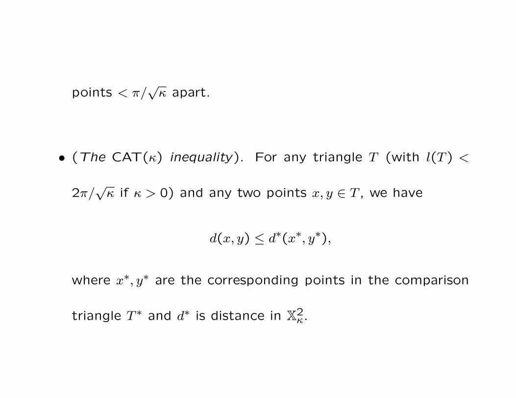
• (The CAT(κ) inequality). For any triangle T (with l(T ) <

2π/√

κ if κ > 0) and any two points x, y ∈ T , we have

d(x, y) ≤ d∗(x∗, y∗),

where x∗, y∗ are the corresponding points in the comparison

triangle T ∗ and d∗ is distance in X2κ.

T T

y

x

y

x

*

*

*

Definition. A metric space X has curvature ≤ κ if the CAT(κ)

inequality holds locally.

Observations. • If κ′ < κ, then CAT(κ′) =⇒ CAT(κ).

• CAT(0) =⇒ contractible.

• curvature ≤ 0 =⇒ aspherical.

Theorem. (Aleksandrov and Toponogov). A Riemannian mfld

has sectional curvature ≤ κ iff CAT(κ) holds locally.

The cone on a CAT(1)-space. The cone on X, denoted

Cone(X), is the quotient space of X × [0,∞) by the equivalence

relation ∼ defined by (x, s) ∼ (y, t) if and only if (x, s) = (y, t) or

s = t = 0. The image of (x, s) in Cone(X) is denoted [x, s]. The

cone of radius r, denoted Cone(X, r), is the image of X × [0, r].

Given a metric space X and κ ∈ R, we will define a metric dκ on

Cone(X). (When κ > 0, the definition will only make sense on

the open cone of radius π/√

κ.) The idea: when X = Sn−1, by

using “polar coordinates” and the exponential map, Cone(Sn−1)

can be identified with (an open subset of) Xnκ. Transporting the

constant curvature metric on Xnκ to Cone(Sn−1), gives a formula

for dκ on Cone(Sn−1). The same formula defines a metric on

Cone(X) for any metric space X. To write this formula recall

the Law of Cosines in X2κ. Suppose we have a triangle in X2

κ with

edge lengths s, t and d and angle θ between the first two sides.

θ

s

t

d

The Law of Cosines:

• in E2:

d2 = s2 + t2 − 2st cos θ

• in S2κ:

cos√

κd = cos√

κs cos√

κt + sin√

κs sin√

κt cos θ

• in H2κ:

cosh√−κd = cosh

√−κs cosh

√−κt+sinh

√−κs sinh

√−κt cos θ

Given x, y ∈ X, put θ(x, y) := min{π, d(x, y)}. Define the metric

d0 on Cone(X) by

d0([x, s], [y, t]) := (s2 + t2 − 2st cos θ(x, y))1/2.

Metrics dκ, κ 6= 0 are defined similarly. Denote Cone(X) equipped

with the metric dκ by Coneκ(X).

Remark. If X is a (n − 1)-dimensional spherical polytope, then

Coneκ(X) is isometric to a convex polyhedral cone in Xnκ.

Proposition. Suppose X is a complete and that any two points

of distance ≤ π can be joined by a geodesic. Then

• Coneκ(X) is a complete geodesic space.

• Coneκ(X) is CAT(κ) if and only if X is CAT(1).

Polyhedra of piecewise constant curvature

We call a convex polytope in Xnκ an Xκ-polytope when we don’t

want to specify n.

Definition. Suppose F is the poset of faces of a cell complex.

An Xκ-cell structure on F is a family (CF )F∈F of Xκ-polytopes

s.t. whenever F ′ < F , CF ′ is isometric to the corresponding face

of CF .

Examples. (i) (Euclidean cell complexes). Suppose a collection

of convex polytopes in En is a convex cell cx in the classical

sense. Then the union Λ of these polytopes is a X0-polyhedral

complex.

(ii) (Regular cells). There are three families of regular polytopes

which occur in each dimension n: the n-simplex, the n-cube and

the n-octahedron. The simplex and the cube have the additional

property that each of their faces is of the same type. Requiring

each cell of a cell cx to be a simplex (resp. cube) we get the

corresponding notion of a simplicial (resp. cubical) cx. In both

cases (n-simplex and n-cube) we can be realize the polytope

as a regular polytope in Xnκ. This polytope is determined, up

to congruence, by its edge length. So, we can define an Xκ-

structure on a simplicial cx or a cubical cx simply by specifying

an edge length.

By now there are many constructions of nonpositively curved PE

polyhedral complexes. In the case of PE cubical complexes there

are the following:

• products of graphs,

• constructions via reflection groups,

• hyperbolizations (e.g. Gromov’s Mobius band procedure),

• certain blowups of RPn and

• many other constructions.

Suppose Λ is a Xκ-polyhedral complex. A path c : [a, b] → Λ is

piecewise geodesic if there is a subdivision

a = t0 < t1 · · · < tk = b s.t. for 1 ≤ i ≤ k, c([ti−1, ti]) is

contained in a single (closed) cell of Λ and s.t. c|[ti−1,ti]is a

geodesic. The length of the piecewise geodesic c is defined by

l(c) :=∑n

i=1 d(c(ti), c(ti−1)), i.e., l(c) := b − a. Λ has a natural

length metric:

d(x, y) := inf{l(c) | c is a piecewise geodesic from x to y }.

(We allow ∞ as a possible value of d.) The length space Λ is

a piecewise constant curvature polyhedron. As κ = +1,0,−1, it

is, respectively, piecewise spherical, piecewise Euclidean or piece-

wise hyperbolic.

Piecewise spherical (= PS) polyhedra play a distinguished role

in this theory. In any Xκ-polyhedral cx each “link” naturally has

a PS structure.

Geometric links. Suppose P is an n-dimensional Xκ-polytope

and x ∈ P . The geometric link, Lk(x, P ), (or “space of direc-

tions”) of x in P is the set of all inward-pointing unit tangent

vectors at x. It is an intersection of a finite number of half-spaces

in Sn−1. If x lies in the interior of P , then Lk(x, P ) ∼= Sn−1,

while if x is a vertex of P , then Lk(x, P ) is a spherical polytope.

Similarly, if F ⊂ P is a face of P , then Lk(F, P ) is the set of

inward-pointing unit vectors in the normal space to F (in the

tangent space of P ).

If Λ is an Xκ-polyhedral complex and x ∈ Λ, define

Lk(x,Λ) :=⋃

x∈P

Lk(x, P ).

Lk(x, P ) is a PS length space. Similarly, Lk(F,Λ) :=⋃

Lk(F, P ).

Theorem. Let Λ be an Xκ-polyhedral complex. TFAE

• curv(Λ) ≤ κ.

• ∀x ∈ Λ, Lk(x,Λ) is CAT(1).

• ∀cells P of Λ, Lk(P,Λ) is CAT(1).

• ∀v ∈ VertΛ, Lk(v,Λ) is CAT(1).

Proof. Any x ∈ Λ has a nbhd isometric to Coneκ(Lk(x,Λ), ε).

Piecewise Euclidean Cubical complexes.

Definition.A simplicial cx L is a flag complex if it has the follow-

ing property: a nonempty finite set of vertices spans a simplex

of L iff any two vertices in the set are connected by an edge.

Examples. The boundary of an m-gon is flag iff m > 3. The

derived cx (= the set of chains) of any poset is a flag cx. Hence,

the barycentric subdivision of any cell cx is a flag cx.

Definition. A spherical simplex is all right if each of its edge

lengths is π/2. (Equivalently, it is all right if each of its dihedral

angles is π/2.) A PS simplicial complex is all right if each of its

simplices is all right.

Example. Since each dihedral angle of a Euclidean cube is π/2,

the link of each cell of a Euclidean cube is an all right simplex.

Hence, the link of any cell in a PE cubical complex is an all right

PS simplicial cx.

Lemma. (Gromov). Let L be an all right PS simplicial cx. Then

L is CAT(1) ⇐⇒ flag cx.

Corollary. A cubical cx is CAT(0) iff the link of each vertex is a

flag cx.

A cubical cx with given link. Suppose L is a flag cx and

S := VertL. Put

S(L) := {T ⊆ S | T is the vertex set of a simplex}

�S := [−1,1]S.

Let XL ⊆ �S be the union of all faces which are parallel to �T

for some T ∈ S(L).

Examples. If L = S0, then XL = ∂�2 = ∂(4-gon) ∼= S1. If

L = ∂(4-gon), then XL = T2 ⊂ ∂�4.

Observations.

• VertXL = {±1}S. So, XL has 2Card(S) vertices. The link of

each vertex is identified with L.

• L a flag cx =⇒ XL nonpositively curved.

• If, in addition, L ∼= Sn−1, then XL is aspherical mfld.

Remark. The group (Z/2)S acts as a reflection group on �S.

Let XL be the universal cover of XL and let WL be the group

of all lifts of elements of (Z/2)S to XL. WL is a “right-angled”

Coxeter group acting as a reflection group on XL. If L is a flag

cx, then XL is CAT(0).