Casualty Actuarial Society E-Forum, Summer 2012
355
Casualty Actuarial Society E-Forum, Summer 2012
Transcript of Casualty Actuarial Society E-Forum, Summer 2012

Casualty Actuarial Society E-Forum, Summer 2012

Casualty Actuarial Society E-Forum, Summer 2012 ii
The CAS E-Forum, Summer 2012
The Summer 2012 Edition of the CAS E-Forum is a cooperative effort between the CAS E-Forum Committee and various other CAS committees, task forces, or working parties. This E-Forum includes papers from two call paper programs and four additional papers.
The first call paper program was issued by the CAS Committee on Reserves (CASCOR). Some of the Reserves Call Papers will be presented at the 2012 Casualty Loss Reserve Seminar (CLRS) on September 5-7, 2012, in Denver, CO.
The second call paper program, which was issued by the CAS Dynamic Risk Modeling Committee, centers on the topic of “Solving Problems Using a Dynamic Risk Modeling Process.” Participants were asked to use the Public Access DFA Dynamo 4.1 Model to illustrate how the dynamic risk modeling process can be applied to solve real-world P&C Insurance problems. The model and manual are available on the CAS Public-Access DFA Model Working Party Web Site.
Committee on Reserves Lynne M. Bloom, Chairperson
John P. Alltop Bradley J. Andrekus Nancy L. Arico Alp Can Andrew Martin Chandler Robert F. Flannery Kofi Gyampo Dana F. Joseph
Weng Kah Leong Glenn G. Meyers Jon W. Michelson Marc B. Pearl Susan R. Pino Christopher James Platania Vladimir Shander Hemanth Kumar Thota
Bryan C. Ware Ernest I. Wilson Jianlu Xu Cheri Widowski, CAS Staff
Liaison
Committee on Dynamic Risk Modeling Robert A. Bear, Chairperson
Christopher Diamantoukos, Vice Chairperson
Jason Edward Abril Fernando Alberto Alvarado Yanfei Z. Atwell Rachel Radoff Bardon Steven L. Berman Morgan Haire Bugbee Alp Can Chuan Cao Patrick J. Crowe Charles C. Emma
Sholom Feldblum Stephen A. Finch Robert Jerome Foskey Bo Huang Ziyi Jiao Steven M. Lacke Zhe Robin Li Christopher J. Luker Xiaoyan Ma Joseph O. Marker
John A. Pagliaccio Alan M. Pakula Ying Pan Theodore R. Shalack Zhongmei Su Min Wang Wei Xie Kun Zhang Karen Sonnet, Staff Liaison

Casualty Actuarial Society E-Forum, Summer 2012 iii
CAS E-Forum, Summer 2012
Table of Contents
2012 Dynamic Risk Modeling Call Papers
Stochastic GMB Methods for Modeling Market Prices James P. McNichols, ACAS, MAAA, and Joseph L. Rizzo, ACAS, MAAA ...................................... 1-18
Effects of Simulation Volume on Risk Metrics for Dynamo DFA Model William C. Scheel and Gerald Kirschner .................................................................................................. 1-22
2012 Reserves Call Papers
A GLM-Based Approach to Adjusting for Changes in Case Reserve Adequacy Decker Exhibits Decker_2009 Claims Decker_All Open Claims Decker_Restated Claims Decker_Script R
Looking Back to See Ahead: A Hindsight Analysis of Actuarial Reserving Methods Susan J. Forray, FCAS, MAAA .................................................................................................................. 1-33
Larry Decker, FCAS, MAAA ..................................................................................................................... 1-17
Back-Testing the ODP Bootstrap of the Paid Chain-Ladder Model with Actual Historical Claims Data Jessica (Weng Kah) Leong, Shaun Wang, and Han Chen ..................................................................... 1-34
The Leveled Chain Ladder Model for Stochastic Loss Reserving LCL1 Model.R LCL2 Model.R LCL1-JAGS LCL2-JAGS
A Practical Way to Estimate One-Year Reserve Risk
Glenn Meyers, FCAS, MAAA, CERA, Ph.D .......................................................................................... 1-33
Robbin Exhibits
A Total Credibility Approach to Pool Reserving Frank Schmid................................................................................................................................................ 1-22
Ira Robbin, Ph.D. ........................................................................................................................................ 1-34
Two Symmetric Families of Loss Reserving Methods Staudt Exhibit
Closed-Form Distribution of Prediction Uncertainty in Chain Ladder Reserving by Bayesian Approach Ji Yao, Ph.D., FIA, CERA .......................................................................................................................... 1-25
Andy Staudt, FCAS, MAAA ...................................................................................................................... 1-29

Casualty Actuarial Society E-Forum, Summer 2012 iv
Additional Papers
Sustainability of Earnings: A Framework for Quantitative Modeling of Strategy, Risk, and Value Neil M. Bodoff, FCAS, MAAA ................................................................................................................. 1-14 A Common Subtle Error: Using Maximum Likelihood Tests to Choose between Different Distributions Gyasi Dapaa .................................................................................................................................................... 1-2
Loyalty Rewards and Gift Card Programs: Basic Actuarial Estimation Techniques Tim A. Gault, ACAS, MAAA, Len Llaguno, FCAS, MAAA, and Martin Ménard, FCAS, MAAA .................................................................................................................. 1-40
A Note on Parameter Risk Gary Venter, FCAS, MAAA, and Rajesh Sahasrabuddhe, FCAS, MAAA ......................................... 1-16
E-Forum Committee Windrie Wong, Chairperson
Cara Blank Mei-Hsuan Chao Mark A. Florenz
Karl Goring Dennis L. Lange
Donna R. Royston, Staff Editor Shayan Sen Rial Simons
Elizabeth A. Smith, Staff Liaison/Staff Editor John Sopkowicz
Zongli Sun Yingjie Zhang
For information on submitting a paper to the E-Forum, visit
http://www.casact.org/pubs/forum/.

Casualty Actuarial Society E-Forum, Summer 2012 1
Stochastic GBM Methods for Modeling Market Prices
James P. McNichols, ACAS, MAAA Joseph L. Rizzo, ACAS, MAAA
______________________________________________________________________________ Abstract
Motivation. Insurance companies and corporations require credible methods in order to measure and manage risk exposures that derive from market price fluctuations. Examples include foreign currency exchange, commodity prices and stock indices. Method. This paper will apply Geometric Brownian Motion (GBM) models to simulate future market prices. The Cox-Ingersoll-Ross approach is used to derive the integral interest rate generator. Results. Through stochastic simulations, with the key location and shape parameters derived from options market forward curves, the approach yields the full array of price outcomes along with their respective probabilities. Conclusions. The method generates the requisite distributions and their parameters to efficiently measure capital risk levels as well as fair value premiums and best estimate loss reserves. The modeled results provide credible estimators for risk based and/or economic capital valuation purposes. Armed with these distributions of price outcomes, analysts can readily measure inherent portfolio leverage and more effectively manage these types of financial risk exposures. Availability. An Excel version of this stochastic GBM method is available from the CAS website, E-Forum section under filename MPiR.xlsm. Keywords. Dynamic risk models; capital allocation; geometric Brownian motion; options market volatility; stochastic process; Markov Process, Itō’s lemma, economic scenario generator.
______________________________________________________________________________
1. PRICE FORECASTING AND ECONOMIC CAPITAL MODELS
There are various methods actuaries may use to generate future contingent market prices. This paper provides the theoretical construct and detailed calculation methodology to model market prices for any asset class with a liquid exchange traded options market (i.e., foreign currency exchange, oil, natural gas, gold, silver, stocks, etc.).
The critical input parameters used in this approach are taken directly from the options market forward curves and their associated volatilities. For example, an insurer wants to determine the range of likely price movements over the next year for the British Pound (GBP) versus the U.S. Dollar (USD). The requisite mean and volatility input assumptions for this approach are readily available from real time financial market sources (i.e., Bloomberg, Reuters, etc.).
There are two fundamentally different approaches to modeling financial related risks, namely, fully integrated and modular.

Stochastic GBM Methods for Modeling Market Prices
Casualty Actuarial Society E-Forum, Summer 2012 2
The fully integrated approach applies an enterprise-wide stochastic model that requires complex economic scenario generator (ESG) techniques and the core inputs are aligned to either real-world or market-consistent parameters.
Real-world ESGs generally reflect current market volatilities calibrated via empirical time series better suited to long-term capital requirements. Market consistent ESGs reflect market option prices that provide an arbitrage-free process geared more toward derivatives and the analytics to manage other capital market instruments. Market consistent ESGs have fatter tails in the extreme right (i.e., adverse) side of the modeled distributions.
Outputs from the ESGs provide explicit yield curves that allow us to simulate fixed income “bond” returns. Interest rates (both real and nominal) are simulated as core outputs and the corresponding equity returns are derived as a function of the real interest rates.
Fully integrated models provide credible market price forecasts but they are complex and require highly experienced analysts to both calibrate the inputs and translate the modeled outputs. The findings derive from an apparent “black box” and are not always intuitive or easily explained to executive managers and third-party reviewers (i.e., rating agencies or regulators).
Proponents of the fully integrated approach assert that it provides an embedded covariance structure, reflecting the causes of dependence. However, a pervasive problem arises when using the fully integrated approach in that no matter how expert the parameterization of the ESG, the model by necessity will reflect an investment position on the future market performance.
Appendix A provides sample input vectors for a typical ESG. A cursory review of the input parameters confirms that any resulting simulation reflects the embedded investment position on the myriad of financial market inputs including short-term rates, long-term rates, force of mean reversion, variable correlations, jump-shift potential, etc.
The approach described in this paper is geared to analyze asset (and liability) risk components that are modeled individually. This is referred to as the modular approach. In this approach capital requirements are determined at the business unit or risk category level (e.g., market, credit and liquidity risk separately) and then aggregated by either simple summation of the risk components (assuming full dependence) or via covariance matrix tabulations (which reflect portfolio effects).
The main advantage of the modular approach is that it provides a simple but credible spreadsheet-based solution to economic capital estimation. Other advantages include ease of implementation, clear and explicit investment position derived from the market and covariance

Stochastic GBM Methods for Modeling Market Prices
Casualty Actuarial Society E-Forum, Summer 2012 3
assumptions, and communication of basic findings.
Consider the financial risk exposure that derives from stock/equity investments. The expected returns originate from non-stationary distributions and the correlation parameters of the various equities likely derive from non-linear systems. Thus, it may be more appropriate to simulate stock prices with a model that eliminates any need to posit future returns but rather simply translates the range of likely outcomes defined by the totality of information embedded within open market trades. Selecting the location and scale parameters from the options markets data yields price forecasts which are devoid of any actuarial bias on the expected “state” of the financial markets. The results provide reliable measures of the range of price fluctuation inherent in these capital market assets.
Financial traders may scrutinize buy/sell momentum and promulgate their own view of the dependency linkages amongst and in between these asset variables, attempting to determine where arbitrage opportunities exist. The net sum of all of the option market trades collectively reflects an aggregate expectation. The market is deemed credible and vast amounts of trade data are embedded within these two key input parameters.
2. PRICE MODELING—THEORY
Markov analysis looks at sequences of events and analyzes the tendency of one event to be followed by another. Using this analysis, one can generate a new sequence of random but related events that will mimic the original. Markov processes are useful for analyzing dependent random events whereby likelihood depends on what happened last. In contrast, it would not be a good way to model coin flips, for example, because each flip of the coin has no memory of what happened on the flip before as the sequence of heads and tails is fully independent.
The Weiner process is a continuous-time stochastic process, W(t) for t ≥ 0 with W(0) = 0 and such that the increment W(t) – W(s) is Gaussian (e.g., normally distributed) with mean = 0 and variance “t - s” for any 0 ≤ s ≤ t, and the increments for non-overlapping time intervals are independent. Brownian motion (i.e., random walk with random step sizes) is the most common example of a Wiener process.
Changes in a variable such as the price of oil, for example, involve a deterministic component, “a∆t”, which is a function of time and a stochastic component, “b∆z”, which depends upon a random variable (here assumed to be a standard normal distribution). Let S be the price of oil at

Stochastic GBM Methods for Modeling Market Prices
Casualty Actuarial Society E-Forum, Summer 2012 4
time = t and let dS be the infinitesimal change in S over the infinitesimal interval of time dt. Change in the random variable Z over this interval of time is dz. This yields a generalized function for determining the successive series of values in a random walk given by dS = adt + bdz, where “a” and “b” may be functions of S and t. The expected value of dz is equal to zero so thus the expected value of dS is equal to the deterministic component, “adt”.
The random variable dz represents an accumulation of numerous random influences over the interval dt. Consequently, the Central Limit Theorem applies which infers that dz has a normal distribution and hence is completely characterized by mean and standard deviation.
The variance of a random variable, which is the accumulation of independent effects over an interval of time is proportional to the length of the interval, in this case dt. The standard deviation of dz is thus proportional to the square root of dt. All of this means that the random variable dz is equivalent to a random variable √W(dt), where W is a standard normal variable with mean equal to zero and standard deviation equal to unity.
Itō’s lemma1
∆X = a(x,t)∆t + b(x,t)∆z
formalizes the fact that the random (Brownian motion) part of the change in the log of the oil price has a variance that is proportional to the square root of this time interval. Consequently, the second order (Taylor) expansion term of the change of the log of the oil price is proportional to the time interval. This is what allows the use of stochastic calculus to find the solutions. The formula for Itō’s Lemma is as follows:
(2.1)
Itō’s Lemma is crucial in deriving differential equations for the value of derivative securities such as options, puts, and calls in the commodity, foreign exchange and stock markets. A more intuitive explanation of Itō’s Lemma that bypasses the complexities of stochastic calculus is given by the following thought experiment:
Visualize a binomial tree that goes out roughly a dozen steps whereby the price at each step is determined by, drift +/- volatility. The average of returns at the end of these steps will be (drift - ½ volatility2) x dt. This is as Itō’s Lemma would expect. However, when you do this averaging to get that number, all of the outcomes (i.e., each of the individual returns) have the same weighting. It is as though you weighted each outcome by its beginning value or price. Since all of the paths started at the same price, it turns out being a simple average (actually, a probability-weighted average with equivalent weights).
1 Kiyoshi Itō (1951). On stochastic differential equations. Memoirs, American Mathematical Society 4, 1–51.

Stochastic GBM Methods for Modeling Market Prices
Casualty Actuarial Society E-Forum, Summer 2012 5
Now run the experiment again, but this time by averaging each of the outcomes by their ending value, which will yield an average mean = (drift + ½ volatility2) x dt. Note the change in the sign from - to +. Consequently, the formula has a minus sign if you use beginning value weights and a plus sign if you use ending value weights. Conceivably, somewhere in the middle of the process (or maybe the average drift of the process) is just the initial drift with no volatility adjustment. Why is this? When you weight by initial price, all of the paths share equal weightings – the bad performance paths carry the same weight as the good, in spite of the fact that they get smaller in relative size. Consequently they are bringing down the average return (thus the “minus ½ sigma2”). The opposite happens when you use ending values as weights, whereby the top paths get really large versus the bottom paths and appear to artificially lift up the returns (in a manner similar to that often observed with some stock indices).
The “reality” is likely somewhere in between, where the number is the initial drift and thus, in this context, Itō’s Lemma is just a weighted averaging protocol.
By inserting Itō’s Lemma into the generalized formula yields a Geometric Brownian Motion (GBM) formula for price changes of the form:
∆S = µS∆t + σS∆z; such that St+1= St + St [µ∆t+σεN(0,1)√∆t].
(2.2)
µ is the expected price appreciation, which can be taken directly from the forward mean curves for any liquid market option (i.e., F/X, Oil, Gold, etc.).
σ is the implied volatility, which can also be taken directly from the option markets price data available on Bloomberg (for example).
S is typically assumed to follow a lognormal distribution and this process is used to analyze commodity and stock prices as well as exchange rates.
A critical input to this market price modeling approach is the interest rate assumption.
A general model of interest rate dynamics may be given by:
∆rt = k(b-rt)∆t + σrγt∆zt. (2.3)
In this method we utilize the Cox-Ingersoll-Ross Model (CIR) as follows:

Stochastic GBM Methods for Modeling Market Prices
Casualty Actuarial Society E-Forum, Summer 2012 6
ri = ri-1 + a(b-ri-1)∆t + σ√ri-1 ε
ri = spot rate at time = i.
ri-1 = spot rate at time = i-1.
a = speed of reversion = 0.01.
b = desired average spot rate at end of forecast: set to spot rate on n-year high-grade, corporate-zero, coupon bond at beginning of forecast; therefore, there is no expectation for a change in the level of yields over the forecast period.
σ = volatility of interest rate process = .85% (the historical standard deviation of the Citigroup Pension Discount Curve n year spot rate).
∆t = period between modeled spot rates in months = 1.
ε = random sampling from a standard normal distribution.
The CIR interest rate model characterizes the short-term interest rate as a mean-reverting stochastic process. Although the CIR model was initially developed to simulate continuous changes in interest rates, it may also be used to project discrete changes from one time period to another.
The CIR model is similar to our market price model in that it has two distinct components: a deterministic part k(b-rt) and a stochastic part σrγt . The deterministic part will go in the reverse direction of where the current short-term rate is heading. That is, the further the current interest rate is from the long-term expected rate, the more pressure the deterministic part applies to reverse it back to the long-term mean.
The stochastic part is purely random; it can either help the current interest rate deviate from its long-term mean or the reverse. Since this part is multiplied by the square root of the current interest rate, if the current interest rate is low, then its impact is minimal, thereby not allowing the projected interest rate to become negative.
3. PRICE MODELING—APPLICATION AND PRACTICE
When implementing this modular approach to model these types of risks, there are key considerations that need be thought through by the actuary. The first and most important is correlation. For this paper, we are assuming independence for simplicity and clarity in the approach. A fully independent view does have value in that it defines a lower boundary region of the result and

Stochastic GBM Methods for Modeling Market Prices
Casualty Actuarial Society E-Forum, Summer 2012 7
a fully dependent view defines an upper boundary. Correlation of financial variables is difficult because they are hard to estimate and can be unstable. For example, consider the chart below, which tracks the relationship between stocks and bonds over time.
Source: GMO as of January 2011.
Another key consideration is the form of the random walk variable. For this example, we are using a normal distribution to model the random walk of the results. The normal distribution is commonly used in financial modeling and does simplify the ideas shown. Depending on the use and application of the model, consideration should be given to this assumption and possible modifications.
The data for this sample exercise is from the forward call options for the British Pound (GBP) versus the U.S. Dollar (USD) currency pair from June 2010 through December 2011. This time interval was selected so that the user can compare the modeled results to the actual results.

Stochastic GBM Methods for Modeling Market Prices
Casualty Actuarial Society E-Forum, Summer 2012 8
GBP v USD Foreign Exchange Futures
Source: (Bloomberg)
Ticker Month Option Mean Volatility
NRM0 Comdty Jun-10 1.4558 14.890 NRN0 Comdty Jul-10 14.920 NRQ0 Comdty Aug-10 14.860 NRU0 Comdty Sep-10 1.4557 14.850 NRV0 Comdty Oct-10 NRX0 Comdty Nov-10 14.830 NRZ0 Comdty Dec-10 1.4556 NRF1 Comdty Jan-11 NRG1 Comdty Feb-11 14.795 NRH1 Comdty Mar-11 1.4555 NRJ1 Comdty Apr-11 NRK1 Comdty May-11 14.730 NRM1 Comdty Jun-11 1.4554 NRN1 Comdty Jul-11 NRQ1 Comdty Aug-11 NRU1 Comdty Sep-11 1.4553 NRV1 Comdty Oct-11 NRX1 Comdty Nov-11 14.760
The first step is to complete the columns for the missing data fields with simple linear interpolation. Other interpolation options are available and should be reviewed when doing the analysis. In this case, a linear interpolation was selected due to the small changes expected in the mean market forward curve. When larger relative price movements are expected, then different interpolations may be used such as geometric means.

Stochastic GBM Methods for Modeling Market Prices
Casualty Actuarial Society E-Forum, Summer 2012 9
Interpolating the missing values generates the following table:
Ticker Month Option Mean Volatility
NRM0 Comdty Jun-10 1.4558 14.890 NRN0 Comdty Jul-10 1.4558 14.920 NRQ0 Comdty Aug-10 1.4557 14.860 NRU0 Comdty Sep-10 1.4557 14.850 NRV0 Comdty Oct-10 1.4556 14.840 NRX0 Comdty Nov-10 1.4556 14.830 NRZ0 Comdty Dec-10 1.4556 14.818 NRF1 Comdty Jan-11 1.4556 14.807 NRG1 Comdty Feb-11 1.4555 14.795 NRH1 Comdty Mar-11 1.4555 14.773 NRJ1 Comdty Apr-11 1.4555 14.752 NRK1 Comdty May-11 1.4554 14.730 NRM1 Comdty Jun-11 1.4554 14.735 NRN1 Comdty Jul-11 1.4554 14.740 NRQ1 Comdty Aug-11 1.4553 14.745 NRU1 Comdty Sep-11 1.4553 14.750 NRV1 Comdty Oct-11 14.755 NRX1 Comdty Nov-11 14.760
The CIR interest rate model is then applied in this example as follows:
r(i) = (ab - (a+y) x r(i-1))dt + srgdZ a = 0.25 b = 0.06
y = 0 s = 0.05 g = 0.50
dt = 1/12 r(0) = 0.0028 (1 month LIBOR).
The above parameterization was provided by life actuarial advisors. Derivation of the CIR parameters is beyond the scope of this paper.

Stochastic GBM Methods for Modeling Market Prices
Casualty Actuarial Society E-Forum, Summer 2012 10
Adding the interest rate calculation expands the table as follows:
Month Market Forward
GBP/USD
Implied Volatility
Interest Rate Z
Jun-10 1.4558 14.89% Jul-10 1.4558 14.92% 0.28% 0.00%
Aug-10 1.4557 14.86% 0.40% 0.00% Sep-10 1.4557 14.85% 0.52% 0.00% Oct-10 1.4556 14.84% 0.63% 0.00% Nov-10 1.4556 14.83% 0.74% 0.00% Dec-10 1.4556 14.82% 0.85% 0.00% Jan-11 1.4556 14.81% 0.96% 0.00% Feb-11 1.4555 14.80% 1.06% 0.00% Mar-11 1.4555 14.77% 1.17% 0.00% Apr-11 1.4555 14.75% 1.27% 0.00% May-11 1.4554 14.73% 1.37% 0.00% Jun-11 1.4554 14.74% 1.46% 0.00% Jul-11 1.4554 14.74% 1.56% 0.00%
Aug-11 1.4553 14.75% 1.65% 0.00% Sep-11 1.4553 14.75% 1.74% 0.00%
Where Z is N(0,1).
This currency model has the following basic structure:
Currency price (end of month) = currency price (beginning of month) x (random walk) x (1 + drift rate adjustment).
The first two elements are typical of standard GBM models. The third component adjusts the model so that the mean of the modeled currencies match the market forward curve. By implementing this adjustment factor, the model is transformed to be price taking. That is, the GBM model is modified to realign the simulated forward means with the current options market expectation2
.
2 The GBM model may be adjusted to use different forward curves than the market aggregate expectation, but then the model would by definition be taking a market pricing position on the variable. However, if that is the case use caution since that analysis may be construed as offering investment advice. Please note the relevant actuarial statements of practice related to investment advice.
Stochastic GBM Methods for Modeling Market Prices
Casualty Actuarial Society E-Forum, Summer 2012 11
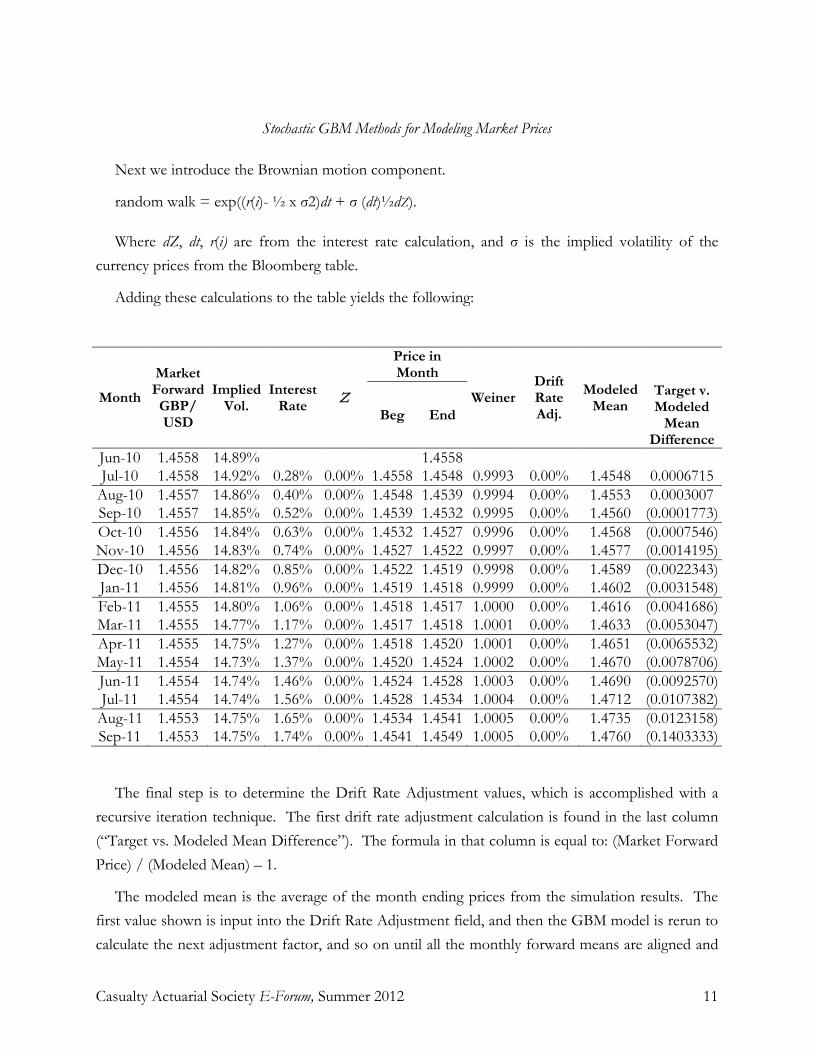
Next we introduce the Brownian motion component.
random walk = exp((r(i)- ½ x σ2)dt + σ (dt)½dZ).
Where dZ, dt, r(i) are from the interest rate calculation, and σ is the implied volatility of the currency prices from the Bloomberg table.
Adding these calculations to the table yields the following:
Month
Market Forward GBP/ USD
Implied Vol.
Interest Rate Z
Price in Month
Weiner Drift Rate Adj.
Modeled Mean
Beg End
Target v. Modeled
Mean Difference
Jun-10 1.4558 14.89% 1.4558 Jul-10 1.4558 14.92% 0.28% 0.00% 1.4558 1.4548 0.9993 0.00% 1.4548 0.0006715
Aug-10 1.4557 14.86% 0.40% 0.00% 1.4548 1.4539 0.9994 0.00% 1.4553 0.0003007 Sep-10 1.4557 14.85% 0.52% 0.00% 1.4539 1.4532 0.9995 0.00% 1.4560 (0.0001773) Oct-10 1.4556 14.84% 0.63% 0.00% 1.4532 1.4527 0.9996 0.00% 1.4568 (0.0007546) Nov-10 1.4556 14.83% 0.74% 0.00% 1.4527 1.4522 0.9997 0.00% 1.4577 (0.0014195) Dec-10 1.4556 14.82% 0.85% 0.00% 1.4522 1.4519 0.9998 0.00% 1.4589 (0.0022343) Jan-11 1.4556 14.81% 0.96% 0.00% 1.4519 1.4518 0.9999 0.00% 1.4602 (0.0031548) Feb-11 1.4555 14.80% 1.06% 0.00% 1.4518 1.4517 1.0000 0.00% 1.4616 (0.0041686) Mar-11 1.4555 14.77% 1.17% 0.00% 1.4517 1.4518 1.0001 0.00% 1.4633 (0.0053047) Apr-11 1.4555 14.75% 1.27% 0.00% 1.4518 1.4520 1.0001 0.00% 1.4651 (0.0065532) May-11 1.4554 14.73% 1.37% 0.00% 1.4520 1.4524 1.0002 0.00% 1.4670 (0.0078706) Jun-11 1.4554 14.74% 1.46% 0.00% 1.4524 1.4528 1.0003 0.00% 1.4690 (0.0092570) Jul-11 1.4554 14.74% 1.56% 0.00% 1.4528 1.4534 1.0004 0.00% 1.4712 (0.0107382)
Aug-11 1.4553 14.75% 1.65% 0.00% 1.4534 1.4541 1.0005 0.00% 1.4735 (0.0123158) Sep-11 1.4553 14.75% 1.74% 0.00% 1.4541 1.4549 1.0005 0.00% 1.4760 (0.1403333)
The final step is to determine the Drift Rate Adjustment values, which is accomplished with a recursive iteration technique. The first drift rate adjustment calculation is found in the last column (“Target vs. Modeled Mean Difference”). The formula in that column is equal to: (Market Forward Price) / (Modeled Mean) – 1.
The modeled mean is the average of the month ending prices from the simulation results. The first value shown is input into the Drift Rate Adjustment field, and then the GBM model is rerun to calculate the next adjustment factor, and so on until all the monthly forward means are aligned and

Stochastic GBM Methods for Modeling Market Prices
Casualty Actuarial Society E-Forum, Summer 2012 12
the differences are all zero.
This can be seen in the following table, shown mid-adjusting:
Month
Market Forward GBP/ USD
Implied Vol.
Interest Rate Z
Price in Month
Weiner Drift Rate Adj.
Modeled Mean
Beg End
Target v. Modeled
Mean Difference
Jun-10 1.4558 14.89% 1.4558 Jul-10 1.4558 14.92% 0.28% 0.00% 1.4558 1.4558 0.9993 0.07% 1.4558 0.0000000
Aug-10 1.4557 14.86% 0.40% 0.00% 1.4558 1.4544 0.9994 (0.04%) 1.4557 0.0000000 Sep-10 1.4557 14.85% 0.52% 0.00% 1.4544 1.4530 0.9995 (0.05%) 1.4557 0.0000000 Oct-10 1.4556 14.84% 0.63% 0.00% 1.4530 1.4516 0.9996 (0.06%) 1.4557 0.0000000 Nov-10 1.4556 14.83% 0.74% 0.00% 1.4516 1.4502 0.9997 (0.07%) 1.4556 0.0000000 Dec-10 1.4556 14.82% 0.85% 0.00% 1.4502 1.4487 0.9998 (0.08%) 1.4556 0.0000000 Jan-11 1.4556 14.81% 0.96% 0.00% 1.4487 1.4485 0.9999 0.00% 1.4569 (0.0009225) Feb-11 1.4555 14.80% 1.06% 0.00% 1.4485 1.4485 1.0000 0.00% 1.4584 (0.0019386) Mar-11 1.4555 14.77% 1.17% 0.00% 1.4485 1.4486 1.0001 0.00% 1.4600 (0.0030773) Apr-11 1.4555 14.75% 1.27% 0.00% 1.4486 1.4488 1.0001 0.00% 1.4618 (0.0043286) May-11 1.4554 14.73% 1.37% 0.00% 1.4488 1.4491 1.0002 0.00% 1.4637 (0.0056489) Jun-11 1.4554 14.74% 1.46% 0.00% 1.4491 1.4496 1.0003 0.00% 1.4657 (0.0070384) Jul-11 1.4554 14.74% 1.56% 0.00% 1.4496 1.4501 1.0004 0.00% 1.4679 (0.0085230)
Aug-11 1.4553 14.75% 1.65% 0.00% 1.4501 1.4508 1.0005 0.00% 1.4702 (0.0101040) Sep-11 1.4553 14.75% 1.74% 0.00% 1.4508 1.4516 1.0005 0.00% 1.4727 (0.0118254)
It is also possible to derive the drift rate adjustment values directly from an analytic approach applied to second differences but the recursive iterative technique was used here for ease of explanation.

Stochastic GBM Methods for Modeling Market Prices
Casualty Actuarial Society E-Forum, Summer 2012 13
After completing the drift rate adjustment process, the results are summarized as follows:
Month
Market Forward GBP/ USD
Implied Vol.
Interest Rate Z
Price in Month
Weiner Drift Rate Adj.
Modeled Mean
Beg End
Target v. Modeled
Mean Difference
Jun-10 1.4558 14.89% 1.4558 Jul-10 1.4558 14.92% 0.28% 0.00% 1.4558 1.4558 0.9993 0.07% 1.4558 0.0000000
Aug-10 1.4557 14.86% 0.40% 0.00% 1.4558 1.4544 0.9994 (0.04%) 1.4557 0.0000000 Sep-10 1.4557 14.85% 0.52% 0.00% 1.4544 1.4530 0.9995 (0.05%) 1.4557 0.0000000 Oct-10 1.4556 14.84% 0.63% 0.00% 1.4530 1.4516 0.9996 (0.06%) 1.4557 0.0000000 Nov-10 1.4556 14.83% 0.74% 0.00% 1.4516 1.4502 0.9997 (0.07%) 1.4556 0.0000000 Dec-10 1.4556 14.82% 0.85% 0.00% 1.4502 1.4487 0.9998 (0.08%) 1.4556 0.0000000 Jan-11 1.4556 14.81% 0.96% 0.00% 1.4487 1.4472 0.9999 (0.09%) 1.4566 0.0000000 Feb-11 1.4555 14.80% 1.06% 0.00% 1.4472 1.4457 1.0000 (0.10%) 1.4555 0.0000000 Mar-11 1.4555 14.77% 1.17% 0.00% 1.4457 1.4441 1.0001 (0.11%) 1.4555 0.0000000 Apr-11 1.4555 14.75% 1.27% 0.00% 1.4441 1.4425 1.0001 (0.13%) 1.4555 0.0000000 May-11 1.4554 14.73% 1.37% 0.00% 1.4425 1.4409 1.0002 (0.13%) 1.4554 0.0000000 Jun-11 1.4554 14.74% 1.46% 0.00% 1.4409 1.4394 1.0003 (0.14%) 1.4554 0.0000000 Jul-11 1.4554 14.74% 1.56% 0.00% 1.4394 1.4378 1.0004 (0.15%) 1.4554 0.0000000
Aug-11 1.4553 14.75% 1.65% 0.00% 1.4378 1.4362 1.0005 (0.16%) 1.4553 0.0000000 Sep-11 1.4553 14.75% 1.74% 0.00% 1.4362 1.4344 1.0005 (0.17%) 1.4553 0.0000000
This modified GBM model has generated a 15-month market aligned foreign exchange price forecast. Each of the month ending values are the means from a probability density function unique to that point in time.
Stochastic GBM Methods for Modeling Market Prices
Casualty Actuarial Society E-Forum, Summer 2012 14
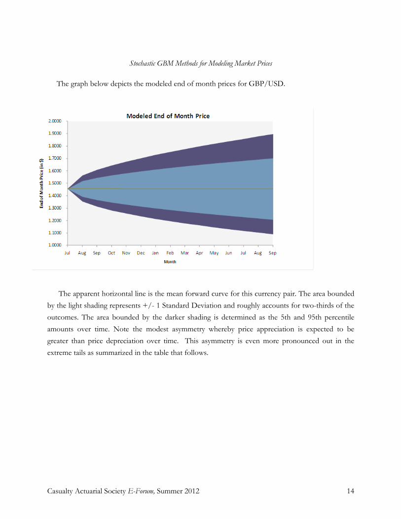
The graph below depicts the modeled end of month prices for GBP/USD.
The apparent horizontal line is the mean forward curve for this currency pair. The area bounded by the light shading represents +/- 1 Standard Deviation and roughly accounts for two-thirds of the outcomes. The area bounded by the darker shading is determined as the 5th and 95th percentile amounts over time. Note the modest asymmetry whereby price appreciation is expected to be greater than price depreciation over time. This asymmetry is even more pronounced out in the extreme tails as summarized in the table that follows.

Stochastic GBM Methods for Modeling Market Prices
Casualty Actuarial Society E-Forum, Summer 2012 15
This table relates the modeled prices to their confidence levels modeled as of July, August, September, and the subsequent quarter ends:
Modeled End of Month Price Confidence
Level Jul-10 Aug-10 Sep-10 Dec-10 Mar-10 Jun-10 Sep-10
0.01% 1.4558 1.2396 1.1606 1.0223 0.9232 0.8566 0.7815 0.05% 1.4558 1.2626 1.1903 1.0502 0.9832 0.8905 0.8372 10.00% 1.4558 1.3762 1.3431 1.2787 1.2321 1.1938 1.1583 20.00% 1.4558 1.4025 1.3806 1.3350 1.3006 1.2720 1.2463 30.00% 1.4558 1.4219 1.4072 1.3763 1.3525 1.3317 1.3118 40.00% 1.4558 1.4386 1.4304 1.4132 1.3991 1.3858 1.3735 50.00% 1.4558 1.4544 1.4531 1.4485 1.4429 1.4384 1.4333 60.00% 1.4558 1.4703 1.4754 1.4849 1.4893 1.4937 1.4949 70.00% 1.4558 1.4876 1.5000 1.5249 1.5404 1.5549 1.5643 80.00% 1.4558 1.5081 1.5294 1.5710 1.6027 1.6286 1.6518 90.00% 1.4558 1.5370 1.5708 1.6409 1.6945 1.7379 1.7813 99.50% 1.4558 1.6252 1.7010 1.8607 1.9980 2.1148 2.2281 99.90% 1.4558 1.6613 1.7553 1.9512 2.1243 2.2844 2.4654
This provides the requisite estimators for risk-based or economic capital valuation purposes. For example, under Solvency II type risk level constraints, the 99.50% confidence level estimate at December is $1.8607. Consequently, the 1:200 stress level risk capital charge for this risk component is required to provide for the net losses that derive from a 28% weakening of the U.S. dollar (= 1.8607/1.4558).
Note: Actuaries must use caution in the display and communication of results from this modified GBM approach. Recall that we seek to provide an unbiased view of the range of future price outcomes. That is, we have not taken an independent view rather we have simply translated the aggregate market expectation.
In the U.S., professionals are licensed specifically to give investment advice to individuals and companies. Although actuaries may present the quantitative results of the GBM model and its effects, use caution in providing any qualitative summarization of the findings. Providing qualitative assessments of the company’s expected future performance may be construed as giving unqualified investment advice.

Stochastic GBM Methods for Modeling Market Prices
Casualty Actuarial Society E-Forum, Summer 2012 16
4. CONCLUSIONS
The method generates probability distribution functions and their parameters to efficiently measure capital risk levels as well as fair value premiums and best estimate loss reserves. The model yields credible estimates of either risk-based or economic capital requirements or both. Equipped with these distributions of price outcomes, analysts can readily measure inherent portfolio leverage and more effectively manage these types of financial risk exposures.
Acknowledgment
The authors acknowledge that this methodology evolved from an initial project that modeled future natural gas prices, which was performed by their actuarial colleague Joe Kilroy. Analytic and editorial assistance has been provided by Jillian Hagan. Appendix A
This exhibit provides a sample of the types of complex inputs required to run economic scenario generators.

Stochastic GBM Methods for Modeling Market Prices
Appendix AESG Prototype: Model ParametersUS Economy : Sample Parameters
Valuation Date 2010.12 Observed Term Structure (linearly interpolated between key rates)1-yr 2-yr 3-yr 4-yr 5-yr 6-yr 7-yr 8-yr 9-yr 10-yr
Projection Period 50 time steps 0.29 0.62 1.06 1.49 1.93 2.20 2.47 2.75 3.02 3.29Time Step 1.000 in years
Real Estate Time Step 1.000 in years 11-yr 12-yr 13-yr 14-yr 15-yr 16-yr 17-yr 18-yr 19-yr 20-yr3.35 3.40 3.46 3.52 3.57 3.63 3.69 3.74 3.80 3.86
Current Risk Free Term StructureCurrent 3-mo rate 0.14% per year 21-yr 22-yr 23-yr 24-yr 25-yr 26-yr 27-yr 28-yr 29-yr 30-yrCurrent 1-yr rate 0.29% 3.91 3.97 4.02 4.08 4.14 4.19 4.25 4.31 4.36 4.42Current 2-yr rate 0.62%Current 5-yr rate 1.93% 31-yr 32-yr 33-yr 34-yr 35-yr 36-yr 37-yr 38-yr 39-yr 40-yr
Current 10-yr rate 3.29% 4.43 4.44 4.45 4.46 4.47 4.47 4.48 4.49 4.50 4.51Current 30-yr rate 4.42%
50-yr Selection 4.60% 41-yr 42-yr 43-yr 44-yr 45-yr 46-yr 47-yr 48-yr 49-yr 50-yr4.52 4.53 4.54 4.55 4.56 4.56 4.57 4.58 4.59 4.60
Real Rate Parameters Inflation ParametersLong INT Reversion Mean 0.0432 Long INT Volatility 2.33% Initial Inflation 0.0148
Long INT Reversion Speed 0.3516 INF Mean 0.0259 INF Volatility 0.0215Short INT Reversion Speed 0.1382 Short INT Volatility 2.18% INF Reversion Speed 0.3852
Large and Small Stock ParametersMedical Inflation Parameters Prob
Initial MED INF 0.0324 Stage0 Mean LS Return 9.00% Stage0 LS Volatility 10.12% stage: 1 0.9760Stage1 Mean LS Return -26.16% Stage1 LS Volatility 27.12% stage: 2 0.8507
MED INF Mean 0.0271MED INF Volatility 0.0088 Stage0 Mean SS Return 8.16% Stage0 SS Volatility 13.86% stage: 1 0.9760
MED INF Reversion Speed 0.0709 Stage1 Mean SS Return 3.60% Stage1 SS Volatility 57.50% stage: 2 0.9000
Dividend ParametersDIV Reversion Mean 4.17% DIV Volatility 0.85%
DIV Reversion 0.13 Correlation ParametersInitial DIV 1.83% Correl LS, SS Regime Switch 90% Dependence method to use?
Correl LS, SS Return 90%Real Estate Parameters Correl DIV, LS -25%
RE Reversion Mean 2.22% RE Volatility 2.82%RE Reversion Speed 0.87 Correl INF, DIV -50%
Initial RE 4.62%Correl Short, Long INT 68%
Correl INF, Short Real INT 2%
Correl INF, MED INF 72%
Rank Dependence
Casualty Actuarial Society Forum Spring, 2012

Stochastic GBM Methods for Modeling Market Prices
Casualty Actuarial Society E-Forum, Summer 2012 17
5. REFERENCES
[1] Ludkovski, Michael and Carmona, Rene, “Spot Convenience Yield Models for Energy Assets,” Contemporary Mathematics, 2004, Vol. 351, 65-82.
[2] Cortazar, G. and Schwartz, E.S., “Implementing a Stochastic Model for Oil Prices,” Energy Economics, 2004, Vol. 25, 215-238.
[3] Schwartz, E.S., “The Stochastic Behavior of Commodity Prices,” The Journal of Finance, 1997, Vol. 52, 923-973. [4] Cox, John C. and Ingersoll Jr., Jonathan E. and Ross, Stephen A., “A Theory of the Term Structure of Interest
Rates,” Econometrica – The Econometric Society, 1985, 385-407. [5] Lo, Andrew W. and Mueller, Mark T., “WARNING: Physics Envy May Be Hazardous to Your Wealth!” MIT
Working Paper Series, 2010, available at SSRN: http://ssrn.com/abstract=1563882. [6] Jorion, Philippe, “Financial Risk Management Handbook,” Global Association of Risk Professionals, 2010. [7] Watkins, Thayer, “Itō’s Lemma” San Jose State University, Department of Economics, available at www.sjsu.edu.
Abbreviations and notations CIR, Cox-Ingersoll-Ross GBP, British pound sterling ESG, economic scenario generator USD, United States dollar GBM, geometric Brownian motion Biographies of the Authors
Jim McNichols is the chief actuarial risk officer at Southport Lane, a New York-based private equity firm. He has a degree in psychology from the University of Illinois with a minor in financial mathematics. He is an Associate of the CAS and a Member of the American Academy of Actuaries. He is participating on the CAS work group reviewing the correlation assumptions in the NAIC RBC calculations, and is a frequent presenter at industry symposia.
Joe Rizzo is a consulting actuary at Aon based in Chicago, IL. His primary areas of focus include stochastic modeling of insurance and financial risks. He has a degree in mathematics from the University of Chicago. He is an Associate of the CAS and a Member of the American Academy of Actuaries.

Casualty Actuarial Society E-Forum, Summer 2012
Effects of Simulation Volume on Risk Metrics for Dynamo DFA Model
By William C. Scheel, Ph.D., DFA Technologies, LLC and Gerald Kirschner, FCAS, MAAA, Deloitte Consulting LLP
_________________________________________________________________________________________ Abstract: Of necessity, users of complex simulation models are faced with the question of “how many simulations should be run?” On one hand, the pragmatic consideration of shortening computer runtime with fewer simulation trials can preclude simulating enough of them to achieve precision. On the other hand, simulating many hundreds of thousands or millions of simulation trials can result in unacceptably long run times and/or require undesirable computer hardware expenditures to bring run times down to acceptable levels. Financial projection models for insurers, such as Dynamo, often have complex cellular logic and many random variables. Users of insurance company financial models often want to further complicate matters by considering correlations between different subsets of the model’s random variables. Unfortunately, the runtime / accuracy tradeoff becomes even larger when considering correlations between variables. Dynamo version 5, written for use in high performance computing (HPC)1
This paper begins by examining the effect that varying the number of simulations has on aggregate distributions of a series of seven right-tailed, correlated lognormal distributions. Not surprisingly, the values were found to be more dispersed for smaller sample sizes. What was surprising was finding that the values were also lower when using smaller sample sizes. Based on the simulations we performed, we conclude that a minimum of 100,000 trials is needed to produce stable aggregate results with sufficient observations in the extreme tails of the underlying distributions.
, as used for this paper, has in excess of 760 random variables, many of which are correlated. We have used this model to produce probability distribution and risk metrics such as Value at Risk (VaR), Tail Value at Risk (TVaR) and Expected Policyholder Deficit (EPD) for a variety of modeled variables. In order to construct many of the variables of interest, models such as Dynamo have cash flow overlays that enable the projection of financial statement accounting structures for the insurance entity being modeled. The logic of these types of models is enormously complex and even a single simulation is time consuming.
Similar conclusions are drawn for the modeled variables simulated with Dynamo 5. Sample sizes under 100,000 produce potentially misleading results for risk metrics associated with projected policyholders surplus. Based on the quantitative values produced by the HPC version of Dynamo 5 used in this article, we conclude that sample sizes in excess of 500,000 are warranted. The reason for the higher number of simulations in Dynamo 5 as compared to the seven variable example is the greater complexity of Dynamo, specifically the much larger number of random variables and the complexity of the correlated interactions between variables. As support for this, we observe that simulated metrics for Policyholders Surplus decreased by 2% to 3% when simulations were increased from 100,000 to 700,000. They decreased by 3% to 6% when simulations were increased from 10,000 to 700,000. _________________________________________________________________________________________
.
1 High performance computing involving the parallelization of the Dynamo model so it would run in computer clusters offers a potential solution to the trade-off between precision and runtime. A small HPC cluster can reduce runtime by 1/3 for 100,000 trials, from about 1.5 hours to 33 minutes.

Effects of Simulations Volume on Risk Metrics for Dynamo DFA Model
Casualty Actuarial Society E-Forum, Summer 2012
CONTENTS
Effects of Simulation Volume on Risk Metrics for Dynamo DFA Model ..................................... 0
Introduction ..................................................................................................................................... 1
Section 1: Comparison of Solvency II and Other Risk Metrics Using Multivariate Simulation of Lognormal Distributions ................................................................................................................. 2
Introduction ................................................................................................................................. 2
Solvency II Risk Aggregation ..................................................................................................... 2
Table 1: QIS5 Correlation Matrix for BSCR ......................................................................... 3
Portfolio Risk Aggregation ......................................................................................................... 3
Solvency II and Portfolio Aggregation ....................................................................................... 5
Table 2: Parameters for Lognormal Distributions ................................................................. 5
Table 3: Correlation Matrix for Lognormal Distributions ..................................................... 5
Table 4: Capital Charges Under Solvency II, Portfolio, and Aggregate Loss Aggregation Methods................................................................................................................................... 6
Aggregate Loss Distribution Using the Iman-Conover Method of Inducing Correlations ........ 6
Table 5: Lognormal Variates Before Induction of Rank Correlation .................................... 7
Table 6: Lognormal Variates After Induction of Rank Correlation ...................................... 7
Sensitivity to Sample Size .......................................................................................................... 9
Table 7: Capital Charges for Different Trial Volumes .......................................................... 9
Figure 1A: High-Variance Lognormal Distribution for Different Sample Sizes ............... 10
Figures 1B and 1C: High-Variance Lognormal Distribution for Different Sample Sizes .... 11
Figure 2: High-Variance Lognormal Original Dynamo 1K Sample Size............................ 12
Figures 3A and 3B: Effect of Sampling Size on Aggregate Loss Distribution ................... 13
Section 2: Effect of Sample Size on Dynamo DFA Variables Distributions .............................. 14
Introduction ............................................................................................................................... 14
High-Volume Sampling Illuminates Extremities in Both Tails of a Distribution .................... 14
Table 8: Effects of Sample Size on Policyholders Surplus....................................................... 16
How Many Simulation Trials Are Enough? ............................................................................. 17
Performance Benchmarks ......................................................................................................... 17
Table 9: Runtimes for HPC Dynamo 5 ..................................................................................... 18
Conclusion .................................................................................................................................... 19
End Notes .................................................................................................................................. 19
Acknowledgement .................................................................................................................... 20

Effects of Simulations Volume on Risk Metrics for Dynamo DFA Model
Casualty Actuarial Society E-Forum, Summer 2012 1
INTRODUCTION
Dynamo is an open access dynamic financial analysis (DFA)2 model built in Microsoft Excel. It is available on the Casualty Actuarial (CAS) web site.3
Participants are encouraged to develop any needed enhancements, such as add-on programs/macros to Dynamo 4.1. This call for papers is intended to foster the use of Dynamo 4.1 and to generate publicly available improvements to the model.
The call paper program (herein after referred to as Call) encouraged model redesign but probably did not anticipate the reformation of the model to run in a high performance computing (HPC) environment.
HPC Dynamo4 still retains standalone properties, but it was redesigned to run with high-volume simulations in the hundreds of thousands5 instead of a few thousand6
In this fashion it is possible to run simulations with as many as 750,000 trials on a moderate-sized cluster in about 30 minutes.
simulations. The model was parallelized and runs in a services oriented architecture (SOA) wherein server computers simultaneously use multiple instances of Excel and the Dynamo model. Empirical probability distributions are built from the simulations being done in parallel across many computers. A pool of such computers is called an HPC cluster. Further, any single computer in the cluster may have many processing units or cores. So, where a cluster has 100 computers, each with four cores, it would be possible to run 400 instances of Excel in parallel.
7
To facilitate the evaluation of what we considered to be interesting and relevant metrics, we extended HPC Dynamo to calculate value at risk (VaR), tail value at risk (TVaR) and expected
The technology affords an interesting opportunity to examine the effects of sample size on various risk metrics being calculated in the Dynamo model.
2 DFA involves simulation to obtain an empirical probability distribution for accounting metrics. As such, an accounting convention such as statutory or GAAP is required. Cash flows are generated for many dependent random variables, and these cash flows are evaluated within the accounting framework. Realizations of financial values from balance sheets or income statements obtained during the simulations are used to construct probability distributions for the financial values. 3 Dynamo model, version 4.1 and documentation can be obtained at: http://www.casact.org/research/index.cfm?fa=padfam. 4 HPC Dynamo version 5.x can be obtained at: http://www.casact.org/research/index.cfm?fa=dynamo. Please note there is a vast amount of both written material and video clips available on-line for version 5.x. This help documentation is directly accessible to users of Dynamo 5x from some new dialogs. 5 HPC Dynamo must be run in Excel 2010 (Microsoft Office version 14). 6 Dynamo 4, the model from which HPC Dynamo 5 was created, can, in theory, also generate several hundred thousand scenarios, but this may not be practical when it takes approximately three hours to run 5,000 simulations. 7 The work done for this paper was generated on two clusters. One had about 240 cores and a smaller one had about 24 cores. There was a mixture of computer types involving both 64- and 32-bit computers. Two operating systems were used: Windows Server 2008 R2 and Windows 7. In our experience, neither of these platforms would be considered large HPC clusters. Each computer supporting the cluster had eight cores. As noted, HPC Dynamo also can be run on single instance of Excel 2010 without HPC functionality.

Effects of Simulations Volume on Risk Metrics for Dynamo DFA Model
Casualty Actuarial Society E-Forum, Summer 2012 2
policyholder deficit (EPD) values for the DFA variables. We have extended HPC Dynamo in this manner in response to the direction that global insurance company solvency and financial regulations (i.e., Solvency II, IFRS) appear to be headed. Other standard statistics also are computed.
SECTION 1: COMPARISON OF SOLVENCY II AND OTHER RISK METRICS USING MULTIVARIATE SIMULATION OF LOGNORMAL DISTRIBUTIONS
Introduction In this section we illustrate sampling phenomena for lognormal distributions that are correlated.
This section is a simplification of the Dynamo 5 example that will be the focus of the next section. In this section we focus on a series of seven lognormally distributed variables. In the next section, we will work with the Dynamo model and its 760 random variables, of which only some are lognormally distributed.
We also use this occasion to review several risk metric constructs, including those being used for Solvency II (S II).
Solvency II Risk Aggregation The Solvency II regime’s standard formula is predicated on risk aggregation of different capital
charges through an approach similar to classical portfolio theory, i.e., there is an assumed reduction in volatility arising from risk diversification. The derivation of the Basic Solvency Capital Requirement (BSCR)8 Table 1 uses a subjective correlation matrix similar to the one shown in to capture this reduction in volatility, and it is calculated using (1).
8 European Commission Internal Market and Services DG, Financial Institutions, Insurance and Pensions, “QIS4 Technical Specifications (MARKT/2505/08), Annex to Call for Advice from CEIOPS in QIS4(MARKT/2504/08),” pp. 286. This document is hereinafter referred to as QIS4. The CEIOPS Solvency II Directive is the globally operative document. It can be found, with highlights for “easy reading” in English, at http://www.solvency-ii-association.com/Solvency_ii_Directive_Text.html. The Committee of European Insurance and Occupational Pensions Supervisors (CEIOPS) web site has the latest rendering of the Solvency II Framework Directive. http://www.europarl.europa.eu/sides/getDoc.do?pubRef=-//EP//TEXT+TA+P6-TA-2009-0251+0+DOC+XML+V0//EN.
Effects of Simulations Volume on Risk Metrics for Dynamo DFA Model
Casualty Actuarial Society E-Forum, Summer 2012 3
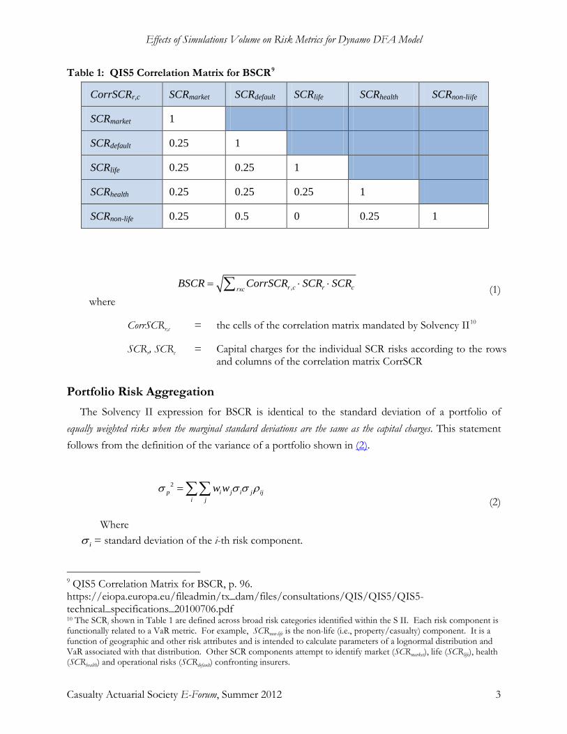
Table 1: QIS5 Correlation Matrix for BSCR9
CorrSCRr,c SCRmarket SCRdefault SCRlife SCRhealth SCRnon-liife
SCRmarket 1
SCRdefault 0.25 1
SCRlife 0.25 0.25 1
SCRhealth 0.25 0.25 0.25 1
SCRnon-life 0.25 0.5 0 0.25 1
,r c r crxcBSCR CorrSCR SCR SCR= ⋅ ⋅∑ (1)
where
CorrSCRr,c = the cells of the correlation matrix mandated by Solvency II10
SCRr, SCRc
= Capital charges for the individual SCR risks according to the rows and columns of the correlation matrix CorrSCR
Portfolio Risk Aggregation The Solvency II expression for BSCR is identical to the standard deviation of a portfolio of
equally weighted risks when the marginal standard deviations are the same as the capital charges. This statement follows from the definition of the variance of a portfolio shown in (2).
2p i j i j ij
i jw wσ σ σ ρ=∑∑
(2)
Where
iσ = standard deviation of the i-th risk component.
9 QIS5 Correlation Matrix for BSCR, p. 96. https://eiopa.europa.eu/fileadmin/tx_dam/files/consultations/QIS/QIS5/QIS5-technical_specifications_20100706.pdf 10 The SCRi shown in Table 1 are defined across broad risk categories identified within the S II. Each risk component is functionally related to a VaR metric. For example, SCRnon-life is the non-life (i.e., property/casualty) component. It is a function of geographic and other risk attributes and is intended to calculate parameters of a lognormal distribution and VaR associated with that distribution. Other SCR components attempt to identify market (SCRmarket), life (SCRlife), health (SCRhealth) and operational risks (SCRdefault) confronting insurers.

Effects of Simulations Volume on Risk Metrics for Dynamo DFA Model
Casualty Actuarial Society E-Forum, Summer 2012 4
When the weights, iw equal 1, equations (1) and (2) are identical. And, iσ = iSCR , when the i-th capital charge in SCR is the standard deviation of some random variable.
The limiting properties of large numbers of component risks may be thought to have the convergence properties of the Central Limit Theorem. Applying this assumption, a VaR measure for a portfolio of risks with mean, pµ , and portfolio standard deviation, pσ can then defined by (3).
*p pVaRα αµ σ= +Θ (3) Where,
αΘ = standard normal value at a cumulative probability of α .
The assumption of a Gaussian process in (3) has rankled many observers. N.N. Taleb, for example, sees “Black Swans” showing up as extreme realizations in risk processes that are distinctly non-normal.11 (3) The chance-constrained metric in for a portfolio of risks may understate the chance-constrained point derived without Gaussian assumptions. We believe Taleb would characterize marginal distributions for many insurance-related loss processes to be Black Swan candidates.
The aggregation method for BSCR indicated in is likely predicated on a methodology in which each component SCR can be thought of as a portfolio component standard deviation. This same approach is widely used among all of the SCRx risk components throughout most S II capital charges.
A solvency capital charge can be a chance-constrained portfolio value such as a multiple of standard deviations as shown in (4).
' * pSCR α σ= Θ (4)
But, the portfolio mean pµ is defined by (5).
p i i
iwµ µ=∑ (5)
So, the portfolio capital charge, SCR’, is given by (6) after substitution of and into and noting that the weights in equal 1.
' pSCR VaRα µ= − (6) And, as noted at the beginning of this section, the Solvency II expression for BSCR is the
standard deviation of a portfolio of equally weighted risks when the marginal standard deviations are the same
11 Black Swan theory explains high-impact, hard-to-predict, and rare events. They arise from non-normal, non-Gaussian expectations. N.N. Taleb, The Black Swan: The Impact of the Highly Improbable, ISBN-13: 9781400063512, 2007, 400 pp. Taleb is not without his critics. A summary of the more cogent ones is found at http://en.wikipedia.org/wiki/Taleb_distribution#Criticism_of_trading_strategies

Effects of Simulations Volume on Risk Metrics for Dynamo DFA Model
Casualty Actuarial Society E-Forum, Summer 2012 5
as the capital charges.
Solvency II and Portfolio Aggregation If we assume that SCR capital charges will, in practice, be larger than the marginal standard
deviations of the SCR components, it means that the SCR, in equation (1) will be larger than iσ in equation (2). This, in turn, would mean that the Solvency II standard formula approach to deriving a capital requirement would be inflated relative to the portfolio approach for defining a capital charge. The capital charges used in S II aggregation are typically more complex measurements than are illustrated in (7). Here the capital charge is a standard normal multiple, αΘ , of the distribution’s standard deviation.
( )i i i i iSCR α αµ σ µ σ= +Θ − = Θ (7)
We will examine this in the context of a portfolio of lognormal random variables with known parameters, { iµ , iσ }. The values of these parameters appear in Table 2. Please note that the term, “Var x” means a lognormally distributed variable and does not mean value at risk or variance. The correlation matrix used both for the S II and portfolio approaches to developing capital charges is shown in Table 3.
Table 2: Parameters for Lognormal Distributions Name Var 1 Var 2 Var 3 Var 4 Var 5 Var 6 Var 7 Risk Model Log
Normal Log Normal
Log Normal
Log Normal
Log Normal
Log Normal
Log Normal
Mean 10000 50000 90000 130000 170000 210000 250000 Standard Deviation
5000 6000 7000 8000 9000 10000 11000
Table 3: Correlation Matrix for Lognormal Distributions Var 1 Var 2 Var 3 Var 4 Var 5 Var 6 Var 7
Var 1 1.0000 0.1315 -0.0986 0.1972 0.3945 0.1972 -0.0723 Var 2 0.1315 1.0000 -0.1972 0.1315 0.3944 0.3945 0.0328 Var 3 -0.0986 -0.1972 1.0000 0.3287 0.1315 0.3945 0.1972 Var 4 0.1972 0.1315 0.3287 1.0000 0.0000 -0.0657 0.1315 Var 5 0.3945 0.3945 0.1315 0.0000 1.0000 0.0328 0.0131 Var 6 0.1972 0.3945 0.3945 -0.0657 0.0328 1.0000 0.5260 Var 7 -0.0723 0.0328 0.1972 0.1315 0.0132 0.5260 1.0000
In the next section we describe aggregation based on a third approach to a capital charge—the difference between VaR and the mean of the multivariate aggregate loss distribution for the lognormal marginal variates described in Table 2 and rank correlated by Table 3.

Effects of Simulations Volume on Risk Metrics for Dynamo DFA Model
Casualty Actuarial Society E-Forum, Summer 2012 6
However, at this point it is instructive to present all three values for these aggregation approaches using this simplified seven variable model. The capital charges appear in Table 4. These capital charges reflect the range of outcomes achieved after 750,000 simulations and taking the .995 percentile of the resulting aggregate distribution.
Table 4: Capital Charges Under Solvency II, Portfolio, and Aggregate Loss Aggregation Methods Method of Aggregation Capital Charge
Aggregate Loss 81,268
Solvency II BSCR 85,654
Portfolio 77,597
The capital charge using the S II methodology exceeds the portfolio approach, and by a sizable margin. Of course, in actual application, this margin will depend on the underlying loss distributions and the correlation matrix.
Aggregate Loss Distribution Using the Iman-Conover Method of Inducing Correlations
The multivariate simulation methods we deploy use the Iman-Conover approach for inducing correlation into independent distributions.12
Table 5
The first step is to simulate values from each of the seven lognormal variables independently of one another to produce a table of n rows by seven columns, where each row represents one scenario in the overall simulation exercise. The second step is to reorder the rows by sorting them from low to high using the values in the first column as the sort field. The matrix being illustrated in show the results of 10 scenarios after reordering them based on the simulated values for Var 1.13
Table 3 The matrix is then shuffled so that the
rearrangement has the Spearman rank correlations shown in . The result of this Iman-Conover induction of correlation into independent distributions appears in Table 6. This approach is particularly useful when correlation is subjective, and the loss processes are developed and parameterized by independent groups of actuaries. It is especially useful for multivariate simulation. Each row of Table 6 contains an n-tuple from a multivariate distribution with Spearman correlations shown in Table 3. The rows are realizations for the seven variables that may be used for different trials in a simulation.
12 The Iman-Conover method is described in the report of the Casualty Actuarial Society’s Working Party on Correlations and Dependencies Among All Risk Sources found at http://www.casact.org/pubs/forum/06wforum/06w107.pdf. Also see Kirschner, Gerald S., Colin Kerley, and Belinda Isaacs, "Two Approaches to Calculating Correlated Reserve Indications Across Multiple Lines of Business," Variance 2:1, 2008, pp. 15-38. 13 The table shows the first ten rows of 25,000 used with the Iman-Conover method.

Effects of Simulations Volume on Risk Metrics for Dynamo DFA Model
Casualty Actuarial Society E-Forum, Summer 2012 7
Table 5: Lognormal Variates Before Induction of Rank Correlation Var 1 Var 2 Var 3 Var 4 Var 5 Var 6 Var 7
1,261 56,244 86,464 139,679 184,313 207,222 220,879
1,350 41,798 82,325 125,670 177,085 201,510 260,059
1,404 53,743 91,548 119,955 167,478 233,410 246,224
1,525 44,553 80,663 142,115 158,827 208,627 235,541
1,620 47,549 77,273 127,529 157,531 197,469 247,044
1,671 47,671 82,639 125,521 183,718 208,845 237,500
1,721 54,840 86,908 132,476 173,432 224,805 265,150
1,734 61,729 83,191 122,804 176,781 201,987 249,738
1,743 55,287 91,678 130,586 169,779 207,816 251,302
1,808 52,759 97,670 133,850 181,218 206,202 266,005
Table 6: Lognormal Variates After Induction of Rank Correlation Var 1 Var 2 Var 3 Var 4 Var 5 Var 6 Var 7 Aggregate
1,261 48,005 97,603 128,608 151,988 212,276 261,124 900,866
1,350 53,071 103,625 121,782 160,720 224,589 259,898 925,035
1,404 40,877 87,598 125,819 153,027 189,504 249,399 847,627
1,525 51,668 96,151 135,583 169,766 191,346 238,395 884,434
1,620 50,617 91,693 127,287 161,166 202,703 255,470 890,555
1,671 50,021 90,844 123,747 149,731 208,077 244,267 868,359
1,721 58,834 83,220 122,938 147,002 219,338 261,585 894,638
1,734 39,731 102,377 129,503 153,077 200,082 244,553 871,057
1,743 38,745 85,285 121,838 143,780 192,489 243,678 827,558
1,808 44,030 89,124 130,296 153,196 190,989 240,596 850,038
Each of the variables in a row of Table 6 is added to produce an observation in the aggregate loss distribution as shown in the final column of each row. This is a multivariate empirical distribution, but there is no available multivariate probability distribution that defines it. That is, the aggregate loss distribution is not constructed with a variance/covariance matrix, and it does not use Pearsonian correlation. Nevertheless, it is an aggregate distribution based on independently derived probability distributions that are observed to have pairwise Spearman rank correlations. It is multivariate in that sense.
We note that this empirical probability distribution is not directly used in Dynamo. Instead, the

Effects of Simulations Volume on Risk Metrics for Dynamo DFA Model
Casualty Actuarial Society E-Forum, Summer 2012 8
multivariate Iman-Conover trials are available for use in Dynamo. The multivariate variables may be used in dependent cells so that a simulation in Dynamo is using random variates that are correlated. It is possible to have many clusters of such correlated variables where each is used for different cell dependencies.14 For example, new business growth among lines of business could be a function of random variables within a pod or cluster that are correlated. 15
DFA variables dependent on them will be generated with the underlying correlation structure of the pod or cluster.
14 The technique is very useful when the underlying correlation structure of a cluster of variables is subjective. It is important to remember, however, that subjective correlations must be reckoned as rank correlations. 15 The term “pod” and “cluster” are used interchangeably in this paper. Each refers to a collection of variables with a correlation structure and multivariate properties defined within the Iman-Conover methodology.

Effects of Simulations Volume on Risk Metrics for Dynamo DFA Model
Casualty Actuarial Society E-Forum, Summer 2012 9
Sensitivity to Sample Size We begin our discussion of simulation volume effects, or sample size effects, with the example in Table 2. Except for small sample sizes, both the S II and portfolio methodologies should be relatively insensitive to sampling error because they depend on first and second moments of distributions and sampling error will rapidly diminish with simulation volume. But, because the underlying distributions are lognormal, we would expect sampling error to have a more profound impact on the variables with the highest second moments, i.e., Var 6 and Var 7. This expectation is confirmed in Table 7.
Table 7: Capital Charges for Different Trial Volumes Capital Charge Methods
Name Mean Standard Deviation
VaR Aggregate Loss Method
Solvency II BSCR Method
Port-folio Method
Trials
Var 1 9,843 4,918 27,280 17,436 1,000 Var 1 9,995 4,993 31,076 21,081 5,000 Var 1 9,928 5,042 31,394 21,467 10,000 Var 1 9,952 5,013 30,702 20,750 25,000 Var 1 9,987 5,051 30,802 20,815 50,000 Var 1 9,990 5,045 30,663 20,673 100,000 Var 1 10,005 5,017 30,261 20,256 250,000 Var 1 10,005 5,006 30,207 20,202 500,000 Var 1 10,004 5,006 30,233 20,228 750,000 ⁞ ⁞ ⁞ ⁞ ⁞ Var 7 250,062 11,305 278,418 28,356 1,000 Var 7 250,128 11,065 279,004 28,877 5,000 Var 7 250,023 10,926 279,204 29,181 10,000 Var 7 250,028 10,937 279,340 29,312 25,000 Var 7 250,000 10,977 279,778 29,778 50,000 Var 7 249,976 10,980 279,963 29,987 100,000 Var 7 249,985 10,997 279,866 29,881 250,000 Var 7 249,986 11,002 279,776 29,790 500,000 Var 7 249,992 11,005 279,722 29,730 750,000 Aggregate 909,344 30,092 987,239 77,895 82,780 78,377 1,000 Aggregate 910,016 29,796 990,112 80,096 85,222 77,357 5,000 Aggregate 909,866 30,135 992,724 82,858 85,856 77,526 10,000 Aggregate 909,972 30,079 990,519 80,547 85,238 77,419 25,000 Aggregate 910,065 30,122 991,457 81,392 86,266 77,683 50,000 Aggregate 909,925 30,063 991,227 81,301 86,184 77,604 100,000 Aggregate 909,979 30,008 991,009 81,030 85,773 77,549 250,000 Aggregate 910,005 30,062 991,133 81,128 85,584 77,588 500,000 Aggregate 910,004 30,045 991,272 81,268 85,654 77,597 750,000

Effects of Simulations Volume on Risk Metrics for Dynamo DFA Model
Casualty Actuarial Society E-Forum, Summer 2012 10
The aggregate distribution capital charge is also affected by sample size as can be seen at the bottom box of Table 7. Visual comparison of the two segments of this box show aggregate capital charges (left column of box) to be both lower and more dispersed for smaller sample sizes. (For example, the average of the Variables and Aggregate column that aggregates for between 1,000 and 50,000 trials is 80,558 as compared to an average of 81,182 for the simulations’ runs that used between 100,000 and 750,000 trials.)
Higher sample sizes for the lognormal distributions result in more observations in the extreme tails. This effect is clearly evident by examining the tail areas of Table 7 where more extreme observations occur with the 750,000 sample size relative to a sample size of only 5,000. The increase in sample size from 100,000 to 750,000 (charts B and C) illustrates how significant shifts in distribution statistics can unfold even when increasing from a comparatively high sample size of 100,000 to extreme sampling sizes such as 750,000. This impact is documented in Table 7 for Var 7. The mean increases from 249,976 to 249,992. However, VaR declines from 279,963 to 279,722.
Figure 1A: High-Variance Lognormal Distribution for Different Sample Sizes16
16 The graphics used in this paper are produced by Dynamo 5 for any simulated variable. The term “Int” in the legend refers to interval. The mean and median intervals are overlaid in their frequency intervals as visualization of where these central tendency measures fall. This information is not particularly useful for this paper, but can be a useful for heavily skewed distributions.

Effects of Simulations Volume on Risk Metrics for Dynamo DFA Model
Casualty Actuarial Society E-Forum, Summer 2012 11
Figures 1B and 1C: High-Variance Lognormal Distribution for Different Sample Sizes17
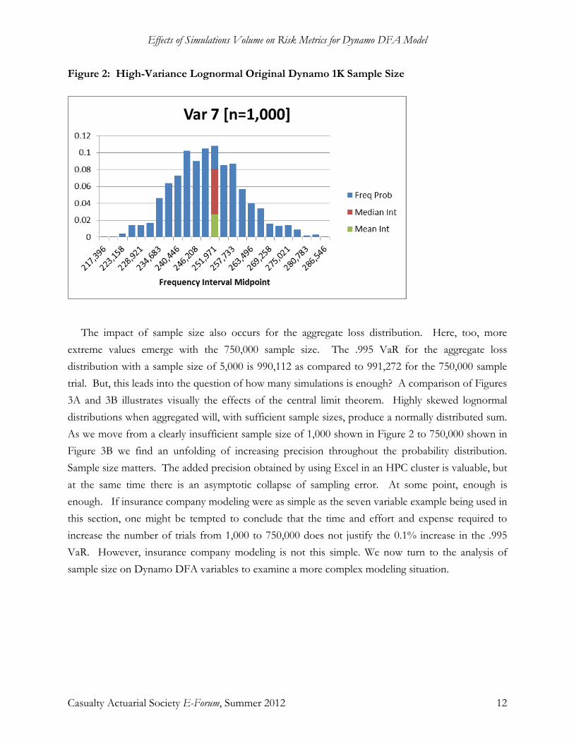
Because prior versions of Dynamo were formulated for sample sizes of only 1,000, the frequency distribution graph for this 1,000 sample size appears in Figure 2. The effects of low sample size are clearly evident both in fewer extreme values and discontinuities in shape of the frequency distribution as compared to the higher sample volumes shown in Figures 1A, 1B, and 1C.
17 The graphics used in this paper are produced by Dynamo 5 for any simulated variable. The term “Int” in the legend refers to interval. The mean and median intervals are overlaid in their frequency intervals as visualization of where these central tendency measures fall. This information is not particularly useful for this paper, but can be a useful for heavily skewed distributions.
Effects of Simulations Volume on Risk Metrics for Dynamo DFA Model
Casualty Actuarial Society E-Forum, Summer 2012 12
Figure 2: High-Variance Lognormal Original Dynamo 1K Sample Size
The impact of sample size also occurs for the aggregate loss distribution. Here, too, more extreme values emerge with the 750,000 sample size. The .995 VaR for the aggregate loss distribution with a sample size of 5,000 is 990,112 as compared to 991,272 for the 750,000 sample trial. But, this leads into the question of how many simulations is enough? A comparison of Figures 3A and 3B illustrates visually the effects of the central limit theorem. Highly skewed lognormal distributions when aggregated will, with sufficient sample sizes, produce a normally distributed sum. As we move from a clearly insufficient sample size of 1,000 shown in Figure 2 to 750,000 shown in Figure 3B we find an unfolding of increasing precision throughout the probability distribution. Sample size matters. The added precision obtained by using Excel in an HPC cluster is valuable, but at the same time there is an asymptotic collapse of sampling error. At some point, enough is enough. If insurance company modeling were as simple as the seven variable example being used in this section, one might be tempted to conclude that the time and effort and expense required to increase the number of trials from 1,000 to 750,000 does not justify the 0.1% increase in the .995 VaR. However, insurance company modeling is not this simple. We now turn to the analysis of sample size on Dynamo DFA variables to examine a more complex modeling situation.

Effects of Simulations Volume on Risk Metrics for Dynamo DFA Model
Casualty Actuarial Society E-Forum, Summer 2012 13
Figures 3A and 3B: Effect of Sampling Size on Aggregate Loss Distribution

Effects of Simulations Volume on Risk Metrics for Dynamo DFA Model
Casualty Actuarial Society E-Forum, Summer 2012 14
SECTION 2: EFFECT OF SAMPLE SIZE ON DYNAMO DFA VARIABLES DISTRIBUTIONS
Introduction Because Excel is used for Dynamo, it can be relatively easy to model complex interactions for a
large number of different DFA variables. Business operations can be modeled with complex cash flow and accounting dependencies using many random variables. Given a set of random variates (Dynamo has in excess of 760 inverse probability functions), a single calculation of the Dynamo workbook produces an empirical realization for the DFA variables being monitored. The parallelization of this process results in these realizations being calculated simultaneously in a computer cluster. Hence, HPC Dynamo can produce probability distributions with 500,000 or more observations in a short time relative to what time would be required were these observations to be done serially in a single instance of Excel. We have seen in the previous section the effects of sample size in the context of a portfolio of lognormal variables, and we now turn to similar experiments for DFA variables.
High-Volume Sampling Illuminates Extremities in Both Tails of a Distribution Often we are more concerned about the extreme tail that represents adverse experience. High-
volume observations enabled by parallelization of the simulation produces enhanced precision throughout the probability distribution. We have more observations at both extremities and, of course, a bevy of additional results that are largely unnecessary in the interior of the distribution. At some point, sampling error affecting moments of the distribution decays to a materially insignificant amount. More simulations do not necessarily produce a better answer. Error in estimating extreme percentiles or even moments required for solvency measurement is materially changed at simulation volumes that might be considered exceedingly large if attempted in a stand-alone computing environment.18
Consider the 0.995 value at risk (VaR) column in
Table 8. This table contains various statistics and risk metrics for the fifth year projection of policyholders’ surplus. This variable is the result of a complex set of cell dependencies in Dynamo. All of the DFA variables that can be assembled using
18 Recall that the original Dynamo only simulated 1,000 observations. And, the results reported by Burkett et al. 2010 were based on 5,000 simulations using Dynamo version 4.1. Version 4.1 required about 2.0078 sec/simulation on a fast desktop computer. It took about three hours to produce 5,000 trials. At that rate, over 16 days would be needed to create 700,000 simulations. In addition to the use of HPC, there have been substantial improvements in Dynamo VBA coding, all of which enhance performance. In a small HPC cluster running 29 simultaneous instances of HPC Dynamo (a core resource allocation one of several types for HPC jobs), three hours is reduced to 1.25 minutes for 5,000 trials. A single trial takes about .015 seconds compared to over two seconds. And, this calculation involves multivariate simulation not available in Dynamo 4.1.

Effects of Simulations Volume on Risk Metrics for Dynamo DFA Model
Casualty Actuarial Society E-Forum, Summer 2012 15
Dynamo have this property. There is no closed form solution for measuring statutory or GAAP variables that are based on cash flows which, by themselves have no closed solution. Simulation is the only viable approach to deriving probability distributions on these DFA variates.
The rows of Table 8 contain results for increasing simulation volumes. Although measurements are shown for samples sizes under 10,000, these small sample sizes have 0.995 VaRs that are heavily affected by the algorithm used to extrapolate this extreme percentile. The number of observations is smaller than the precision sought for that extremity. This algorithmic effect can be seen in the bowing of the VaRs between 1,000 and 10,000 observations. Beginning at 10,000 observations, however, a secular decline in VaR values occurs with increased simulation counts. The VaR for the 10,000 trial simulation is 12,898. By the time the 700,000 trial simulation is run, the VaR has reduced to 12,130, i.e., a 6% reduction. This 6% reduction is very likely to be considered material when considering minimum capital requirements. Similarly, one observes a 1% reduction in the VaR when moving from 500,000 to 700,000—this change may, too, be considered material.
Statistics relating to central tendency, such as the mean and median, also change, and change materially when moving from 100,000 to 700,000 trials. Both the mean and median are reduced by 2.3%.
The effect of moving from 10,000 to 700,000 trials is large. And, it is larger for extreme percentiles...profoundly so. VaR is reduced by about 6%. The mean is reduced by about 2%. The benefit of increased trial counts is higher at distribution tails than for central tendency.

Effects of Simulations Volume on Risk Metrics for Dynamo DFA Model
Casualty Actuarial Society E-Forum, Summer 2012 16
Table 8: Effects of Sample Size on Policyholders Surplus19
Observations
Mean Standard Deviation
Coef of Variation Minimum Maximum
.010 Percentile Median
.990 Percentile EPD20 TVaR 21 VaR 22
1,000
21,762 3,277 0.151 11,609 30,682 13,550 21,856 28,604 9,290 3,401 12,188 5,000 21,678 3,238 0.149 9,311 33,723 13,824 21,719 28,827 9,391 3,415 12,891
10,000 21,607 3,222 0.149 6,975 33,723 13,769 21,697 28,667 9,203 3,399 12,898 20,000 21,547 3,231 0.150 6,975 33,723 13,644 21,643 28,511 9,171 3,382 12,749 30,000 21,519 3,237 0.150 -1,368 33,723 13,592 21,599 28,597 9,224 3,379 12,653 40,000 21,496 3,242 0.151 -1,368 33,723 13,522 21,572 28,619 9,201 3,373 12,515 50,000 21,478 3,248 0.151 -1,368 33,918 13,531 21,547 28,628 9,204 3,368 12,545 60,000 21,463 3,252 0.152 -1,621 33,918 13,507 21,533 28,634 9,194 3,365 12,572 70,000 21,445 3,259 0.152 -1,621 33,918 13,471 21,521 28,662 9,180 3,359 12,545 80,000 21,437 3,262 0.152 -1,621 33,918 13,448 21,520 28,651 9,149 3,356 12,503 90,000 21,429 3,262 0.152 -1,621 33,918 13,427 21,513 28,645 9,142 3,354 12,515
100,000 21,419 3,263 0.152 -1,621 33,918 13,409 21,504 28,632 9,131 3,351 12,494 200,000 21,340 3,278 0.154 -15,412 34,368 13,318 21,432 28,584 9,071 3,331 12,405 250,000 21,312 3,283 0.154 -15,412 34,447 13,264 21,399 28,559 9,063 3,324 12,359 300,000 21,287 3,285 0.154 -15,412 34,447 13,260 21,375 28,537 9,049 3,318 12,347 400,000 21,242 3,289 0.155 -15,412 34,643 13,215 21,332 28,512 9,026 3,308 12,317 500,000 21,201 3,295 0.155 -15,412 34,643 13,150 21,291 28,480 9,003 3,298 12,257 600,000 21,161 3,301 0.156 -31,483 34,643 13,097 21,251 28,456 8,984 3,289 12,195 700,000 21,116 3,308 0.157 -31,483 34,643 13,043 21,207 28,427 8,960 3,278 12,130
19 Table 8 illustrates the type of statistics available for all Dynamo-simulated variables. Statutory policyholders surplus for a company with two multi-peril and workers compensation lines of business is illustrated in the open source version of Dynamo 5. This is the source of Table 8, and the lognormal distributions used in Section 1 are among the Dynamo distributions used for variates leading to policyholders surplus. It is available on Casualty Actuarial Society web site http://www.casact.org/research/index.cfm?fa=dynamo. 20 Expected Policyholder Deficit for area bounded between 0.5 and 0.8. 21 Tail Value at Risk for tail above 0.995. 22 Value at Risk for 0.995.

Effects of Simulations Volume on Risk Metrics for Dynamo DFA Model
Casualty Actuarial Society E-Forum, Summer 2012 17
How Many Simulation Trials Are Enough? The results for various statistics and risk metrics shown in Table 8 are clearly impacted by
simulation volume. The importance of a high performance computational environment becomes apparent when attempting to pragmatically answer the question of how many trials is enough. In all of metrics in Table 8, we believe a minimum of 100,000 trials is essential to reduce sampling error to an acceptable minimum level. A strong argument can be made for 700,000 trials. The precision obtained when increasing trial count from 100,000 to 700,000 is a difference of 1.88%, 2.20%, and 2.90%, respectively for expected policyholder deficit, tail value at risk and value at risk. There is no risk metric that is immune from a reduction in sampling error achieved with high-volume simulations.
An HPC approach is highly desirable when simulation volumes reach a range of 100,000 and a necessity when they reach 700,000. A single machine just cannot run fast enough to produce this volume of trials. Precision is achieved in a reasonable time frame only by using high-performance computing.
Performance Benchmarks The runtimes shown in Table 9 reflect calculation overhead relating to calculation of multivariate
pods and statistics/risk metrics. The former occurs at the beginning of each HPC job whereas the latter is incurred at job conclusion. Both of them are done on the client computer. The simulations are done on cluster compute nodes, and they involve primarily the generation of random variables, including the lookup of pre-calculated multivariate simulations that were done by the client when the Excel workbook is prepared for upload to the HPC cluster. In order to improve cluster performance, the simulations received by the client from the compute nodes is written to disk rather than inserted immediately into the client worksheet. When the simulations are complete, this file is read and, at that time, the results are written to the simulation output worksheet. For trial counts in excess of 100,000, the insertion of new rows of data into this output area is a slow operation in Excel. This transfer and the subsequent derivation of statistics add time to the end of the job.
The calculation of multivariate simulation variates, particularly for large simulation counts can be relatively slow. The setup of multivariate random variables using the Iman-Conover methodology requires a Choleski decomposition and a potentially large matrix inversion. When the trial count approaches 100,000, this process is relatively slow because it has not been converted yet into compiled code in HPC Dynamo 5. The Iman-Conover code implementation relies on VBA code. Counts over 100,000 are commensurately slower. Similarly, when the trial counts are large the development of statistics and risk metrics after simulations are complete is also relatively slow. The effects of this overhead are apparent in Table 9. The simulations per second decline somewhat with

Effects of Simulations Volume on Risk Metrics for Dynamo DFA Model
Casualty Actuarial Society E-Forum, Summer 2012 18
increased simulation count.
Table 9: Runtimes for HPC Dynamo 523
Trials
Small HPC Cluster Runtime (27 core allocations over 5 nodes)24
Approximate Runtime Standalone (2 cores single node)
10000 1.15 mins 9 mins
25000 3.43 mins 22.5 mins
50000 9.53 mins 45 mins
100000 33.27 mins 90 mins
500000 407.34 mins ???
700000 946.56 mins ???
The potential power of parallelization and use of a computer cluster can be seen in Table 9. The runtimes using HPC are faster than running on a single computer and, for the larger sample sizes most appropriate for risk metrics the improvement is dramatically so. HPC cluster performance is never linear, and this is evident in Table 9. A substantial overhead occurs in loading an instance of Excel for each core and when the Dynamo workbook is opened by each core instance. There is an additional overhead for higher simulation volumes because of additional system activity in scheduling those simulations across the cluster. When a simulated array of DFA variables is completed by a cluster computer, it must be inserted into the client Excel instance of Dynamo. This too is an additional and significant source of overhead directly related to simulation volume. Pragmatically, even if the small cluster were only two times faster than a single computer for very high simulation volumes, 0.66 days for 700,000 simulations of 74 DFA variables is better than an estimated 1.31 days it might otherwise take for a single computer.
23 The runtimes are for the simulation of 74 DFA variables and two multivariate pods. The time includes preparation of statistical and risk metric output for these variables. When simulation counts are large, the derivation of multivariate deviates takes more time because of sorting requirements involved in the Iman-Conover method. The runtimes are for the complete setup of multivariate values, simulations and derivation of statistics and risk metrics for all DFA variables. 24 This is a very small HPC cluster. The performance gains over a single actuarial workstation are even more impressive given that they are derived from a modest extension of the workstation from 1 (standalone) to 5 nodes (computers). However, several of the additional computers are multiple-core servers.

Effects of Simulations Volume on Risk Metrics for Dynamo DFA Model
Casualty Actuarial Society E-Forum, Summer 2012 19
CONCLUSION
This paper has used HPC Dynamo to identify the effects of sample size on DFA variable probability distributions. The impact of sampling error is so profound that a dilemma occurs. The number of trials needed to reduce the material impact of sampling error on risk metrics exceeds 100,000 trials. On a single computer the runtime becomes prohibitively large. The parallelization of simulations and their calculation on many simultaneous instances of Excel necessitates added expenditure for the cluster computers and multiple copies of Excel required for each of the node computers in the cluster. And, of course, each cluster computer must have an operating system. HPC Excel requires at least one server computer. The dilemma arises in that a reduction in sampling error to materially insignificant levels requires more trials that only can be achieved for increased costs.25
We have set out to answer the question of “How many simulations is enough.” It is unlikely that any analysis of DFA variables involving less than 100,000-500,000 trials should be used, particularly when these variables are used to measure the effects of capital attribution or are used as proxies for risk-bearing measurements.
In the first part of this paper, the effects of sample size were examined within the context of aggregate probability distributions for correlated lognormal variables. This measurement was done using an aggregate loss distribution. We showed material impacts of sample size on the aggregate loss distribution and risk metrics such as Solvency II-styled calculations that rely on the properties of the aggregate loss distribution. The same observation applies across both parts of this paper—simulation volumes must be large and will require the use of high-performance computing. DFA variables in Dynamo can be constructed from any statutory, GAAP or cash flow variable. The probability distributions for these variables are highly sensitive to the number of simulation trials used in their estimation. Expected policyholder deficit, tail value at risk and value at risk decreased by 2% to 3% when simulations were increased from 100,000 to 700,000. They decrease by three to 6% when simulations were increased from 10,000 to 700,000. Variables such as VaR that are used in solvency compliance metrics have extreme sensitivity to simulation volume.
End Notes In their 2009 paper, “A Holistic Approach to Setting Risk Limits,” Burkett et al. observed that
Dynamo 4.1 contained some inaccurate reconciliations among balance sheet, income statement, and cash flow statement values. Those inconsistencies remain in the Dynamo 5 model that has been
25 At the time of this writing, HPC Excel running in Azure is only possible using an on-premise head node. The head node is a server computer. This computer is required if Azure is used and deployed in the VM Node role required for HPC Excel.

Effects of Simulations Volume on Risk Metrics for Dynamo DFA Model
Casualty Actuarial Society E-Forum, Summer 2012 20
used for this paper. In the authors’ views, these inconsistencies do not change the conclusions we have reached in this paper, but we do recommend that any user of Dynamo consider the potential effect of these inconsistencies on the results being produced and the usage of the results by their organization.
Acknowledgement About Deloitte Deloitte refers to one or more of Deloitte Touche Tohmatsu Limited, a U.K. private company limited by guarantee, and its network of member firms, each of which is a legally separate and independent entity. Please see www.deloitte.com/about for a detailed description of the legal structure of Deloitte Touche Tohmatsu Limited and its member firms. Please see www.deloitte.com/us/about for a detailed description of the legal structure of Deloitte LLP and its subsidiaries. Certain services may not be available to attest clients under the rules and regulations of public accounting. This publication contains general information only and Deloitte is not, by means of this publication, rendering accounting, business, financial, investment, legal, tax, or other professional advice or services. This publication is not a substitute for such professional advice or services, nor should it be used as a basis for any decision or action that may affect your business. Before making any decision or taking any action that may affect your business, you should consult a qualified professional advisor. Deloitte, its affiliates, and related entities shall not be responsible for any loss sustained by any person who relies on this publication

Casualty Actuarial Society E-Forum, Summer 2012 1
A GLM-Based Approach to Adjusting for Changes in Case Reserve Adequacy
Larry Decker, FCAS, MAAA ______________________________________________________________________________
Abstract This paper will address adjusting incurred loss triangles for changes in case reserve adequacy. This proposal is an attempt to improve upon the traditional Berquist-Sherman Method by using a generalized linear model of case reserves as the basis for restating case reserves at earlier evaluations rather than using average case reserves as the basis. Keywords: Case reserve adequacy; generalized linear modeling; reserving; reserve strengthening
______________________________________________________________________________
1. INTRODUCTION
This paper describes a method for adjusting incurred loss triangles for changes in case reserve adequacy using a Generalized Linear Model (GLM). In a similar fashion to the Berquist-Sherman method for adjusting case reserves (BSM), this method restates case reserves at prior evaluations based on the case reserves of the most recent evaluation. Instead of simply using the average case reserves of the most recent evaluation of a column to represent current claims handling practice as the BSM does, this method uses a generalized linear model of reserves using all open claims at the most recent evaluation. The individual case reserve by claim at the most recent evaluation is the dependent variable and various characteristics of each claim are the independent variables for the GLM. Independent variables could be any variable that could be associated with a claim such as claimant age, geographic region, pricing variables from the associated policy, etc.
The resulting GLM is understood to be a model of current claims handling practice. Once developed, the GLM is applied to all individual open claims at current and prior evaluations to restate their reserves to what they would be under the current practice. These restated reserves are then aggregated and added to the corresponding paid losses at each evaluation in order to create the restated loss incurred triangle. At this point typical loss development methods can be applied.
1.1 Objective This method has several advantages over the BSM:
In practice the application of the BSM often results in loss development patterns that are “wavy” with alternating large jumps and drops. This is due to variation in average claim reserves by accident year. In any given column of the triangle, if the most recent point is from an accident year that by chance has types of claims with higher reserves, the whole column will be restated at a high level

A GLM Based Approach to Adjusting for Changes in Case Reserve Adequacy
Casualty Actuarial Society E-Forum, Summer 2012 2
using this most recent point as the basis. The converse would be true for a column where the most recent point is from an accident year with low reserves. The alternation of columns with high and low restated reserves across the triangle creates the “wavy” effect. It can be difficult to select a smooth loss development pattern under this scenario.
In the proposed method, the reserves for each accident year and evaluation in the triangle are restated using the characteristics of the claims open for that accident year at that evaluation. This is an improvement in accuracy compared to using one accident year with potentially different claim characteristics to restate the reserves of a different accident year. An accident year with types of claims with higher reserves will typically have higher reserves in every column. This leads to consistency across each accident year row of the triangle, eliminating the “wavy” effect.
In the BSM, for each of the points in a given column of the triangle, the average reserves of the most recent accident year in that column is the only source for information to represent the level of case reserves under the current claims handling practice. By applying the GLM, the proposed method uses information from all of the open claims in all columns at the most recent evaluation.
The exercise of developing the GLM for case reserves at the current evaluation increases understanding of the drivers of case reserve levels. If certain characteristics lead to higher case reserve levels, there is potential for the claims department to target claims with those characteristics in order to mitigate losses. The results of the model can also suggest changes to be made to rates.
1.2 Outline The remainder of the paper proceeds as follows. Section 2 will describe in more detail the steps
of the GLM based method. An example of the method using simulated data will be provided in Section 3. Also in Section 3, the BSM will be applied to the same data in order to compare the two methods.
2. STEPS OF THE GLM-BASED METHOD
2.1 Data Collection Three sets of data need to be created:

A GLM Based Approach to Adjusting for Changes in Case Reserve Adequacy
Casualty Actuarial Society E-Forum, Summer 2012 3
Paid Losses
Paid losses will be needed to add to the restated case reserves in order to create the incurred loss triangle. The paid losses can be aggregated as a paid loss triangle. Individual claim detail is not necessary unless partial paid losses for individual claims are used as one of the independent variables.
Earlier Evaluation Points
The data required to restate the triangle once the GLM is created includes the independent variables for every claim that was ever open at an evaluation date included in the loss development triangle. This data set should include a record for each open claim and evaluation date. The independent variables listed in each record should be what they were as of the evaluation date for that record. For each such claim, it would also be helpful to have the historical case reserve to assist in testing the GLM. Time-sensitive variables, such as claimant age at the evaluation date, should be recalculated for each prior evaluation date.
Most Recent Evaluation Point
The data required to create the GLM include the case reserve and any characteristics to be used as independent variables for every claim open as of the most recent evaluation period (latest “diagonal”). As mentioned above, independent variables could be any variables that could be associated with a claim such as claimant age, geographic region, pricing variables from the associated policy, etc. In lines of business with partial payments, paid losses may also be a helpful variable. Care must be taken to choose characteristics that are available for open claims at prior evaluation dates. This data set should include a record for each claim open as of the most recent evaluation period.
2.2 Create the GLM Use the data set from the most recent evaluation point mentioned in Section 2.1 above to create
a GLM using case reserves as the dependent variable and the characteristics selected to be the independent variables. In-depth instruction regarding the creation of GLMs is beyond the scope of this paper. Two excellent resources for those desiring a better understanding of GLMs can be found in the references section. For “hands on” instruction, the CAS Predictive Modeling Limited Attendance Seminar is highly recommended.

A GLM Based Approach to Adjusting for Changes in Case Reserve Adequacy
Casualty Actuarial Society E-Forum, Summer 2012 4
2.3 Use the GLM to Restate Historical Case Reserves by Claim Apply the GLM created in Section 2.2 to the second data set from Section 2.1 to restate the case
reserves for all of the claims that were open during any of the evaluation dates in the triangle. If accident year and/or age of claim are used as independent variables, inflation trend may be reflected in the model. In this case, the selection of a separate trend factor and de-trending may not be required.
If the actual case reserves for each open claim at each evaluation are available, compare them to the restated case reserves. Differences should make sense based on conversations with claims management regarding why the case reserve adequacy has changed. Claims with large unexplained differences should be scrutinized in the claims system in order to discover similarities between them that may lead to potential new independent variables for the GLM. If found, they can be used to enhance the GLM and reduce the differences.
It is possible that the new independent variables found cannot be successfully added to the GLM if they cannot pass testing for significance. In this case, the actual historical case reserve may be a better representation of the claim than the restated modeled case reserves and should be substituted as the restated case reserve. This is especially true if discussions with claims management indicate that the causes of change in the level of case reserve adequacy do not apply to these claims.
One situation that may arise is that there are claims that have been settled with payment, yet remain open with a small case reserve for follow-up items such as legal expenses, unpaid medical bills not part of the settlement, etc. The model may generate a large case reserve on these claims based on their characteristics. If settled claims can be identified, an attempt should be made to add a settlement variable to the GLM. If this attempt is unsuccessful, it is best to leave them at the actual case reserve rather than using the modeled reserve.
2.4 Create the Restated Incurred Loss Development Triangle Sum the restated case reserves from Section 2.3 by accident year and age to create a restated case
reserve triangle. Add these to the paid loss triangle from Section 2.1 to create the restated case incurred triangle. This triangle can now be used for typical loss development methods.

A GLM Based Approach to Adjusting for Changes in Case Reserve Adequacy
Casualty Actuarial Society E-Forum, Summer 2012 5
3. EXAMPLE OF THE GLM-BASED METHOD
3.1 Overview The example provided below is intended to illustrate the steps of the GLM based method and is
somewhat simple for the sake of brevity. It is not intended to prove the superiority of the proposed method over the BSM, but simply to disclose the new method.
3.2 Creation of Simulated Data The data for this example was created using the CAS Public Loss Simulator Model (CASPLSM).
This model is publicly available software that can be used for the simulation of loss data. More information on this model can be found at http://www.casact.org/research/lsmwp/lossinstruct/index.cfm?fa=main. The data was completely fabricated to represent a generic line of business. The parameters discussed below were not based on any empirical data. The only rationale for the selection of these parameters is to simply provide simulated data that looks as realistic as possible. Data was simulated for accident years 2000 – 2009 with annual evaluations. Each claim had the following characteristics used as independent variables: Injury, Gender, and Claimant Age at time of accident. Injury includes the following levels: Back, Burn, Spinal Cord, and Other. For accident year 2000 the average severities selected for these injury types were:
Back 200
Burn 100
Spinal Cord 500
Other 50
For subsequent accident years, a 5% inflation trend was applied. These severities were adjusted by the following relativities for Gender and Claimant Age:
Male 0.80
Female 1.20
Age Under 16 0.50

A GLM Based Approach to Adjusting for Changes in Case Reserve Adequacy
Casualty Actuarial Society E-Forum, Summer 2012 6
Age 16-25 0.75
Age 26-45 1.00
Age 46-65 1.50
Age 66 and Over 2.00
For each accident year there are 40 different combinations of Injury, Gender, and Claimant Age, resulting in 40 different expected severities. These severities were used to create parameters for the CASPLSM in combination with the following coefficients of variation by injury:
Back 2.0
Burn 0.5
Spinal Cord 2.0
Other 1.0
Gamma distributions were used for simulating size of loss in the CASPLSM simulations, which require shape and scale parameters. The shape parameter is calculated as the reciprocal of the square of the coefficient of variation. The scale parameter is the expected severity divided by the shape parameter.
For accident year 2000, mean claim counts were randomly assigned to each of the 40 claim types with an expected total number of claims of 600. This number was selected in consideration of finding a balance between having enough data to create an analysis and keeping the simulated data small enough to be manageable. For subsequent accident years the total number of claims was increased using a 10% growth rate (e.g., 660 for 2001, 726 for 2002). The resulting mean claim counts were used as parameters for the Poisson distributions used for frequency in the CASPLSM simulations.
The CASPLSM includes specification of parameters for setting the level of case reserve adequacy. Two simulations were run for each accident year, one with a lower level of case reserve adequacy and one with a higher level of case reserve adequacy. Output from the CASPLSM includes transaction level detail of when payments were made and case reserves were changed. This output was consolidated by claim and evaluation date (12/31/2000 through 12/31/2009) to create the data

A GLM Based Approach to Adjusting for Changes in Case Reserve Adequacy
Casualty Actuarial Society E-Forum, Summer 2012 7
used in the example. For evaluations 12/31/2000 through 12/31/2008, the output from the simulations with a lower level of case reserve adequacy were used. For the 12/31/2009 evaluation, the simulations with a higher level of case reserve adequacy were used (thus creating the change in adequacy that is the subject of this paper).
The GLM modeling is done in R. R is a free software environment for statistical computing and graphics that is gaining wide use among actuaries. R was used in order to allow anyone to step through the GLM used in the example. R is readily available for download from http://www.r-project.org. For those unfamiliar with R, a good place to start is the “An Introduction to R” paper in the “Manuals” section of the above website. The Casualty Actuarial Society Open-Source Software Committee maintains a website, http://opensourcesoftware.casact.org, with some useful resources for R. Also, the CAS Predictive Modeling Limited Attendance Seminar provides a “hands-on” opportunity for using R and assumes no previous R experience. See Appendix A for the R code that created the GLM used in this paper.
3.3 Electronic Files Provided • 2009 Open Claims.csv: Claim detail for all open claims as of 12/31/2009. This is the data
set for the most recent evaluation point described in Section 2.1.
• All Open Claims.csv: Claim detail for all open claims as of all evaluations. This is the data set for earlier evaluation points described in Section 2.1 above.
• call_paper_script.R: This is the R script used to create the GLM from “2009 Open Claims.csv” and apply it to the data in “All Open Claims.csv” in order to restate the case reserves.
• Restated Claims.csv: This file has the restated case reserves generated by “call_paper_script.R”. This is one column of numbers with an entry for each record in “All Open Claims.csv”.
• Exhibits.xls: This Excel workbook uses the raw data and the restated reserves to create the restated case incurred triangle and results for the GLM method. The restated case incurred triangle and results for the BSM are also created in this file. This file has the following tabs:
• Exhibits: This tab includes the paid loss triangle, reserves and development factors generated by the GLM Method, and the calculations and development factors derived

A GLM Based Approach to Adjusting for Changes in Case Reserve Adequacy
Casualty Actuarial Society E-Forum, Summer 2012 8
for the same claim data set using the BSM formatted for printing as (Appendix B).
• WORK: This tab includes the work to support the Exhibits tab.
• All Data Table: This tab includes all paid losses and case reserves by claim for all evaluations. This tab is the source for the paid loss triangle mentioned in Step 2.1.
• All Open and Restated Reserves: This tab includes the data from “All Open Claims.csv” in columns A thru M. Column N has the restated reserves from “Restated Claims.csv”.
3.4 Applying the Steps Step 2.1 has already been completed by the provision of the electronic files mentioned above.
Steps 2.2 and 2.3 are completed in R using the commands in the “call_paper_script.R” file. This script uses the files “2009 Open Claims.csv” and “All Open Claims.csv” as inputs and creates the file “Restated Claims.csv.” A detailed description of each of the commands in this script is provided in Appendix A. As indicated in Section 2.2, in depth instruction on the creation of GLMs is beyond the scope of this paper. However, it is worth mentioning some important steps in a typical GLM process that were omitted to keep the example simple. These include:
• Initial review of potential independent variables for inclusion in the model. There are often a large number of potential independent variables that must be limited to a manageable number for modeling. An initial step is often performing “one-way” analyses on potential independent variables.
• Creating hold out samples from the data for the purpose of testing the model.
• Testing the independent variables for significance.
• Performing analysis of the residuals and other model diagnostics in order to determine the appropriateness of the model.
Step 2.4 is completed in the Exhibits.xls file. The data from “All Open Claims.csv” is copied into the “All Open and Restated Reserves” tab and the restated reserves from “Restated Claims.csv” are copied into the same tab. The first pivot table in the WORK tab is the paid loss triangle created from the data in the “All Data Table” tab. The second pivot table is the triangle of case reserves restated from the GLM method. These two triangles are added together to create the restated incurred loss triangle.

A GLM Based Approach to Adjusting for Changes in Case Reserve Adequacy
Casualty Actuarial Society E-Forum, Summer 2012 9
This triangle is now used to create report to report factors based on weighted averages. The tail factor used was calculated by dividing the actual ultimate losses for accident year 2000 obtained from the simulation process by the case incurred losses for accident year 2000. The resulting report to ultimate factors are applied to actual case incurred losses to calculate ultimate losses by accident year. The paid loss, restated reserve, and restated incurred triangles are shown on Page 1 of Appendix B along with the calculations used to arrive at an estimate of ultimate losses.
3.5 Calculation of the Berquist-Sherman Method Appendix B Pages 2 and 3 show the calculations for the BSM. On Page 2 the average case
reserves are calculated and a trend factor of 1.05 selected. On Page 3 average case reserves are restated by de-trending the average case reserves for the latest diagonal. These average case reserves are then multiplied by the open claims and added to paid losses to create the restated incurred loss triangle. This triangle is now used to create report to report factors based on weighted average. The tail factor is the same as the one used for the GLM method. The resulting report to ultimate factors are applied to case incurred losses to calculate an estimate of ultimate losses by accident year.
4. RESULTS AND DISCUSSION
The results of the proposed GLM method and the BSM can be compared in Appendix B. Rows labeled “Actual Ultimate” and “Actual RTRs” are included in Appendix B and, due to the process used for simulating the data, the ultimate losses are known. The actual RTR factors are weighted averages calculated based on a triangle created by using the simulations with a higher level of case reserve adequacy for all evaluations. The GLM method can be observed to provide ultimate losses and RTRs that are closer to the actual values than the BSM method. This is not necessarily a fair comparison since the independent variables used in the GLM model were also used in the creation of the simulated data.
However, examination of the BSM example illustrates the “wavy” effect described in the introduction. In particular, there is a huge drop in RTR factors at age 5 and a jump at age 6. In comparing accident year 2004 average case reserves for ages 1 to 5 to other accident years, it is clear that 2004 is a “good” year with claims that have relatively lower severity than other years. In the BSM the average case reserve for 2004 at age 6 is the basis for the estimates of the average case reserves for all of the prior years at age 6. This causes the restated losses for these prior years to be understated leading to a drop in the RTR at age 5 and a jump in the RTR at age 6. This shows a

A GLM Based Approach to Adjusting for Changes in Case Reserve Adequacy
Casualty Actuarial Society E-Forum, Summer 2012 10
weakness in the BSM, as it assumes the same mix of claim characteristics for all accident years.
The “wavy” effect is not observed with the proposed GLM method because it reflects variation of claim characteristics by accident year, assuming predictive claim characteristics can be found and incorporated into the GLM as independent variables.
It should be noted that the use of accident year as an independent variable in the GLM method accounted for the inflation trend in the data. In this case, the selection of a separate trend factor was unnecessary.
5. CONCLUSIONS
The GLM method proposed in this paper offers a new approach to adjusting loss development triangles for a change in case reserve adequacy. In cases where detailed claim and claimant information is available for evaluation points at current and historical periods, this approach may offer a significant improvement over the BSM.
For high frequency, low severity lines of business, the proposed method should work well, since enough data should be available in order to create an accurate GLM. On the other hand, the GLM method may not produce a significant improvement over the BSM, since the weaknesses inherent in the BSM are not as pronounced in these lines. There is less variation in average claim reserves by accident year and the latest accident year in a given column of the triangle is more likely to be representative of prior accident years.
For low frequency, high severity lines of business, it may be more challenging to create an accurate GLM due to the limited amount of data. However, for these lines the GLM method offers the most opportunity for improvement over the BSM due to the increased variation in average claim reserves by accident year.
Acknowledgment
The author acknowledges the management of Midwest Employers Casualty Company for their support for this project. The author would also like to thank Chris Platania and Jon Michelson for their thoughtful suggestions for improving this paper. Supplementary Material
See section 3.2

A GLM Based Approach to Adjusting for Changes in Case Reserve Adequacy
Casualty Actuarial Society E-Forum, Summer 2012 11
Appendix A Appendix A includes the R script used for this paper.
Appendix B Appendix B includes the calculations described in Section 3.
6. REFERENCES
James R. Berquist and Richard E. Sherman “Loss Reserve Adequacy Testing: A Comprehensive Systematic Approach” PCAS 1977, Vol. LXIV, 123-184)
Duncan Anderson, et al. “A Practitioner’s Guide to Generalized Linear Models” CAS Discussion Paper Program 2004, 1-116)
Piet de Jong and Gillian Z. Heller Generalized Linear Models for Insurance Data 2008, Cambridge University Press W.N. Venables, D.M. Smith, and the R Development Core Team “An Introduction to R” 2012, R Development Core
Team Abbreviations and notations BSM, Berquist-Sherman method for adjusting case reserves GLM, generalized linear models RTR, Report to Report CAS, Casualty Actuarial Society CASPLSM, CAS Public Loss Simulator Model
Biography of the Author
Larry Decker is a senior actuarial analyst at Midwest Employers Casualty Company. His duties include modeling and support for reserving. Prior to joining Midwest Employers in 2005 he had over 15 years of personal lines experience in various pricing and reserving roles. He has a bachelor’s degree in System Science and Mathematics from Washington University in St. Louis. He is a Fellow of the CAS and a Member of the American Academy of Actuaries.

A GLM Based Approach to Adjusting for Changes in Case Reserve Adequacy
Casualty Actuarial Society E-Forum, Summer 2012 12
Appendix A: R Script Used to Create GLM Example
The “statmod” package is required for the Tweedie distribution as it is used for the GLM error distribution in this example. It must be installed in order for the command loading it to work. The command below loads this package. # load the package with the Tweedie distribution. This may have to be installed.
library(statmod)
The next command reads the “2009 Open Claims.csv” file into the data frame “Open2009”. Note that the path must be changed to the location of this file. Also note that the forward “/” must be used in the path since “\” is a special character in R. #Read in the 2009 open claims data (latest evaluation)
Open2009<-read.csv("c:/callpaper/2009 Open Claims.csv",sep=",")
The next two commands set the levels to be used as the base levels for injury and claimant age. This was done in order to set the base levels to be the same as those used to create the simulated data. When “real” data is used the base level is typically set to be the one with the largest number of observations. This step is not necessary to run the model, but if it is omitted R uses the first level in alphabetical order as the base level. This can create erratic results if this level has a low number of observations. #Change the base level for Injury and Clmt.Age
Open2009$Injury<-relevel(Open2009$Injury,"Other")
Open2009$Clmt.Age<-relevel(Open2009$Clmt.Age,"26-45")
The next command creates the GLM “OpenGLM” using Reserve as the dependent variable and accident year, gender, claimant age, and injury as the independent variables. The Tweedie distribution is used with variance power equal to 2 and link power equal to zero. This distribution was selected because it seems to work well in a variety of situations. The link power of zero results in a log link, which is often used. The variance power of 2 was selected based on judgment and was subject to less analysis and testing than would usually be done in practice. #Create the GLM
OpenGLM<-glm(Reserve~Accident.Year+Gender+Clmt.Age+Injury,
data=Open2009, family=tweedie(var.power=2,link.power=0))
The next command shows a summarization of the GLM with coefficient estimates and goodness-of-fit statistics. This completes Step 2.2.
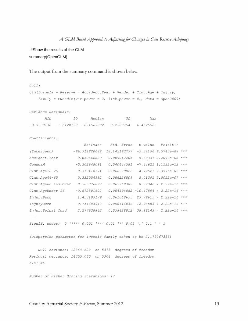
A GLM Based Approach to Adjusting for Changes in Case Reserve Adequacy
Casualty Actuarial Society E-Forum, Summer 2012 13
#Show the results of the GLM
summary(OpenGLM)
The output from the summary command is shown below. Call:
glm(formula = Reserve ~ Accident.Year + Gender + Clmt.Age + Injury,
family = tweedie(var.power = 2, link.power = 0), data = Open2009)
Deviance Residuals:
Min 1Q Median 3Q Max
-3.9339130 -1.6120198 -0.4569802 0.2380754 6.4625565
Coefficients:
Estimate Std. Error t value Pr(>|t|)
(Intercept) -96.914820682 18.142193797 -5.34196 9.5743e-08 ***
Accident.Year 0.050666820 0.009042205 5.60337 2.2070e-08 ***
GenderM -0.302648091 0.040644581 -7.44621 1.1132e-13 ***
Clmt.Age16-25 -0.313418574 0.066329026 -4.72521 2.3575e-06 ***
Clmt.Age46-65 0.332054992 0.066226809 5.01391 5.5052e-07 ***
Clmt.Age66 and Over 0.585376897 0.065969382 8.87346 < 2.22e-16 ***
Clmt.AgeUnder 16 -0.672501602 0.064194852 -10.47594 < 2.22e-16 ***
InjuryBack 1.453199179 0.061068655 23.79615 < 2.22e-16 ***
InjuryBurn 0.754684943 0.058116036 12.98583 < 2.22e-16 ***
InjurySpinal Cord 2.277638842 0.058428812 38.98143 < 2.22e-16 ***
---
Signif. codes: 0 ‘***’ 0.001 ‘**’ 0.01 ‘*’ 0.05 ‘.’ 0.1 ‘ ’ 1
(Dispersion parameter for Tweedie family taken to be 2.179067388)
Null deviance: 18844.622 on 5373 degrees of freedom
Residual deviance: 14355.060 on 5364 degrees of freedom
AIC: NA
Number of Fisher Scoring iterations: 17

A GLM Based Approach to Adjusting for Changes in Case Reserve Adequacy
Casualty Actuarial Society E-Forum, Summer 2012 14
Step 2.3 is completed in the next two steps. In this command “All Open Claims.csv” is read in to the data frame “OpenAll”. #Read in the data for all of the open claims at all evaluations
OpenAll<-read.csv("c:/callpaper/All Open Claims.csv",sep=",")
In the next command the GLM “OpenGLM” is applied to this data set to obtain the restated reserves in the “OpenRestated” array. #Obtain the restated values for all of the open claims at all evaluations
OpenRestated<-predict(OpenGLM,newdata=OpenAll,type='response')
The next command sets the option for how many digits will be written. A few more than the default of 7 was desired. #set the number of digits to be written out
options("digits"=10)
The final command writes the restated reserves to the file “Restated Claims.csv”. #Write the restated values to a file
write(OpenRestated,"c:/callpaper/Restated Claims.csv",sep=",",ncolumns=1)

A GLM Based Approach to Adjusting for Changes in Case Reserve Adequacy
Casualty Actuarial Society E-Forum, Summer 2012 15
Appendix B: Ultimate Losses Using GLM Based Method and Berquist-Sherman Method Page 1
PAID LOSSESAge
Accident Year 1 2 3 4 5 6 7 8 9 102000 11,859 24,975 44,312 60,972 73,490 82,477 94,199 98,595 101,078 105,4672001 13,916 46,989 71,368 86,520 103,005 120,614 134,482 146,104 157,3912002 10,726 26,710 47,271 78,252 118,524 135,367 146,345 156,6312003 6,386 20,919 46,540 61,770 92,823 111,674 128,6992004 14,668 23,949 37,889 85,848 100,959 120,8042005 6,117 26,869 58,434 110,236 145,0302006 22,453 59,637 95,0942007 19,338 60,820 112,0362008 28,672 90,4112009 54,424
GLM BASED METHOD
Restated ReservesAge
Accident Year 1 2 3 4 5 6 7 8 9 102000 204,127 196,620 163,974 131,223 105,900 83,082 67,252 51,749 44,014 30,6812001 285,696 266,167 218,144 181,627 145,959 119,263 91,578 69,423 51,8772002 257,074 250,931 212,368 168,226 123,193 95,581 73,843 57,0672003 269,409 250,686 204,074 162,771 126,908 96,332 76,4842004 282,101 266,584 225,028 178,128 145,528 115,9112005 354,078 333,633 276,596 222,185 176,4042006 381,173 357,873 307,448 254,8822007 508,896 490,213 410,4552008 708,427 653,4112009 764,927
Restated IncurredAge
Accident Year 1 2 3 4 5 6 7 8 9 102000 215,986 221,595 208,286 192,195 179,390 165,559 161,451 150,344 145,092 136,1482001 299,612 313,156 289,512 268,147 248,964 239,877 226,060 215,527 209,2682002 267,800 277,641 259,639 246,478 241,717 230,948 220,188 213,6982003 275,795 271,605 250,614 224,541 219,731 208,006 205,1832004 296,769 290,533 262,917 263,976 246,487 236,7152005 360,195 360,502 335,030 332,421 321,4342006 403,626 417,510 402,542 254,8822007 528,234 551,033 522,4912008 737,099 743,8222009 819,351
Report to Report FactorsAge
Accident Year 1 2 3 4 5 6 7 8 92000 1.026 0.940 0.923 0.933 0.923 0.975 0.931 0.965 0.9382001 1.045 0.924 0.926 0.928 0.964 0.942 0.953 0.9712002 1.037 0.935 0.949 0.981 0.955 0.953 0.9712003 0.985 0.923 0.896 0.979 0.947 0.9862004 0.979 0.905 1.004 0.934 0.9602005 1.001 0.929 0.992 0.9672006 1.034 0.964 0.6332007 1.043 0.9482008 1.009
Wtd Avg 1.018 0.936 0.888 0.954 0.951 0.963 0.954 0.969 0.938 0.958Cumulative 0.614 0.603 0.644 0.725 0.760 0.799 0.830 0.870 0.899 0.958Case Incurred 843,192 712,769 535,091 335,810 329,777 208,510 212,847 221,876 217,227 131,181Ultimate 517,568 429,608 344,502 243,598 250,715 166,613 176,671 193,104 195,199 125,622Actual Ultimate 574,974 492,017 364,166 278,450 266,085 178,339 180,345 201,849 197,819 125,622Difference -57,406 -62,409 -19,664 -34,852 -15,370 -11,726 -3,674 -8,745 -2,620 0Actual RTR 0.996 0.931 0.927 0.945 0.956 0.957 0.974 0.968 0.978 0.958

A GLM Based Approach to Adjusting for Changes in Case Reserve Adequacy
Casualty Actuarial Society E-Forum, Summer 2012 16
Appendix B: Ultimate Losses Using GLM Based Method and Berquist-Sherman Method Page 2
BERQUIST-SHERMAN METHOD
Case ReservesAge
Accident Year 1 2 3 4 5 6 7 8 9 102000 65,093 63,292 51,526 41,860 34,300 29,156 21,467 18,619 15,540 25,7142001 110,790 103,274 90,761 79,514 67,777 57,927 45,727 39,413 59,8362002 104,149 105,569 96,960 78,728 54,134 43,471 37,343 65,2452003 110,813 107,534 94,923 84,790 66,479 55,609 84,1482004 93,277 95,674 88,720 60,268 52,178 87,7062005 147,552 146,874 132,356 102,975 184,7472006 146,093 138,584 117,743 225,5742007 197,305 200,143 423,0552008 265,840 622,3582009 788,768
Open Claim CountAge
Accident Year 1 2 3 4 5 6 7 8 9 102000 606 569 479 385 310 245 191 148 123 882001 656 620 511 416 330 265 209 154 1082002 724 706 601 464 350 274 223 1722003 753 700 580 466 365 274 2112004 740 712 614 494 404 3152005 939 895 740 603 4622006 939 885 743 6072007 1,169 1,116 9352008 1,221 1,1582009 1,318
Average ReservesAge
Accident Year 1 2 3 4 5 6 7 8 9 102000 107 111 108 109 111 119 112 126 126 2922001 169 167 178 191 205 219 219 256 5542002 144 150 161 170 155 159 167 3792003 147 154 164 182 182 203 3992004 126 134 144 122 129 2782005 157 164 179 171 4002006 156 157 158 3722007 169 179 4522008 218 5372009 598
Latest 598 537 452 372 400 278 399 379 554 292Selected Trend 1.05

A GLM Based Approach to Adjusting for Changes in Case Reserve Adequacy
Casualty Actuarial Society E-Forum, Summer 2012 17
Appendix B: Ultimate Losses Using GLM Based Method and Berquist-Sherman Method Page 3
BERQUIST-SHERMAN METHOD (Continued)
Restated Avg. Reserve (Latest Average Reserve Detrended)Age
Accident Year 1 2 3 4 5 6 7 8 9 102000 386 364 322 277 313 229 345 344 528 2922001 405 382 338 291 329 241 362 361 5542002 425 401 355 306 345 253 380 3792003 447 421 372 321 363 265 3992004 469 442 391 337 381 2782005 492 464 410 354 4002006 517 487 431 3722007 543 512 4522008 570 5372009 598
Restated IncurredAge
Accident Year 1 2 3 4 5 6 7 8 9 102000 245,637 231,956 198,339 167,736 170,619 138,598 159,999 149,517 165,979 131,1812001 279,635 283,798 243,900 207,649 211,571 184,352 210,083 201,739 217,2272002 318,653 309,850 260,337 220,112 239,427 204,565 231,044 221,8762003 342,660 315,689 262,442 211,365 225,211 184,331 212,8472004 361,660 338,763 277,875 252,361 254,820 208,5102005 468,437 442,384 362,129 323,653 329,7772006 507,889 491,053 415,267 225,5742007 653,894 632,044 535,0912008 724,593 712,7692009 843,192
Report to Report FactorsAge
Accident Year 1 2 3 4 5 6 7 8 92000 0.944 0.855 0.846 1.017 0.812 1.154 0.934 1.110 0.7902001 1.015 0.859 0.851 1.019 0.871 1.140 0.960 1.0772002 0.972 0.840 0.845 1.088 0.854 1.129 0.9602003 0.921 0.831 0.805 1.066 0.818 1.1552004 0.937 0.820 0.908 1.010 0.8182005 0.944 0.819 0.894 1.0192006 0.967 0.846 0.5432007 0.967 0.8472008 0.984
Wtd Avg 0.963 0.839 0.860 1.035 0.835 1.143 0.953 1.091 0.790 0.958Cumulative 0.541 0.562 0.670 0.778 0.752 0.900 0.787 0.826 0.757 0.958Ultimate 456,304 400,580 358,407 276,699 248,009 187,698 167,563 183,202 164,409 125,622Actual Ultimate 574,974 492,017 364,166 278,450 266,085 178,339 180,345 201,849 197,819 125,622Difference -118,670 -91,437 -5,759 -1,751 -18,076 9,359 -12,782 -18,647 -33,410 0Actual RTR 0.996 0.931 0.927 0.945 0.956 0.957 0.974 0.968 0.978 0.958

Casualty Actuarial Society E-Forum, Summer 2012 1
Looking Back to See Ahead: A Hindsight Analysis of Actuarial Reserving Methods
Susan J. Forray, FCAS, MAAA ________________________________________________________________________ Abstract
Thirty actuarial reserving methods are evaluated empirically against an extensive database of Schedule P data. The metric of method skill is used to evaluate the historical performance of the methods. Results are provided by company size and line of business. The effect of correlation on the usefulness of additional methods is considered. Results suggest the use of several methods not common in actuarial practice, as well as a refinement of weights typically assigned to the more common methods.
Keywords. reserving; reserving methods; management best estimate; suitability testing.
1. INTRODUCTION
Actuarial reserve analyses typically rely on a number of different estimation methods to develop indicated ultimate loss1. The paid and incurred (i.e., paid plus case) chain ladder methods are surely the most common. Other actuarial reserving methods2
include the following:
• Backward Recursive • Claims Closure • Benktander • Frequency/Severity • Berquist-Sherman • Hindsight Outstanding/IBNR • Bornhuetter-Ferguson • Incremental Additive • Brosius • Incremental Multiplicative • Cape Cod • Loss Ratio • Case Development Factor • Munich Chain Ladder
Of course most of these methods have both paid and incurred versions and many have several other variations as well.
Oftentimes, these methods diverge significantly, and actuarial judgment is used in selecting ultimate loss. A need exists for empirical evidence to support the use of particular methods over others.
1 Within this monograph the term “loss” should be taken to refer either just to loss or more generally to loss and ALAE. 2 Descriptions of these methods as used within the current analysis can be found in Appendix A.

Looking Back to See Ahead: A Hindsight Analysis of Common Actuarial Methods
Casualty Actuarial Society E-Forum, Summer 2012 2
1.1 Outline The remainder of this paper proceeds as follows. Section 2 will provide an overview of the
analysis, including the data available as well as a discussion of the metric. Section 3 will discuss the results of the analysis, including results by company size and line of business. Section 4 will discuss the effect of correlation between methods on the results and the practical implications of this correlation. Section 5 will provide additional discussion on the approach to the analysis, and, in particular, the metric selected. Lastly, Section 6 will offer some conclusive remarks.
2. OVERVIEW OF ANALYSIS
2.1 Data for Analysis The current analysis relies on a large database of Schedule P3
triangular data. Thirty methods, as listed in Appendix A, were applied to the triangular data given within Schedule P to develop indications of ultimate loss by coverage year and method for each line of business available for a given property & casualty insurance company. The most recent evaluation date available at the time of the analysis was December 31, 2010. Consequently this functioned as the date as of which “actual” ultimate loss would be determined. Indications based on data as of prior valuations were then evaluated against the ultimate loss as of this most recent valuation date. This is summarized in Table 1.
TABLE 1 VARIABLE COMBINATIONS FOR ULTIMATE LOSS DEVELOPMENT
Variables Companies Lines of Business Methods
Evaluation Dates
Accident / Report Years
Description P&C Writers
10-year triangle Schedule P lines
As Above, Including Variations
1996-2009 10 Years Preceding Evaluation Date
Approximate Number 3,100 16 30 14 10
3 Schedule P is a section of the U.S. Statutory Annual Statement in which triangular data, including paid and case reserve loss and ALAE as well as closed and open claim counts, are reported. The current analysis uses only those lines of business for which 10-year triangles are provided in Schedule P.

Looking Back to See Ahead: A Hindsight Analysis of Common Actuarial Methods
Casualty Actuarial Society E-Forum, Summer 2012 3
Note that only individual companies were considered within this analysis. Company groups were excluded as their data would have overlapped with that of the individual writers. The indicated ultimate loss has been developed under an automated procedure for each of the above combinations for which data is available. Details of the calculations for each method are given in Appendix A.
In theory, the above combinations for which data is available could have resulted in as many as 208 million records of ultimate loss indications. In practice, most companies do not write many of the lines of business. Data for many of the companies is not available at all evaluation dates and, even when it is, the Schedule P triangles are occasionally found to be inconsistent at different evaluation dates and consequently unusable. Ultimate loss indications are available for 49 million of the above variable combinations.
2.2 Method Skill The concept of method skill is a recent introduction to the actuarial profession, having first been
discussed by Jing, Lebens, and Lowe in [8]. It will be discussed at a high level here. However, it may be useful for the reader to have further understanding of the calculation of method skill as applied to the analysis at hand. This is provided in Appendix B.
The skill of method m at development age d is calculated as
Skillm(d) = 1 – msem(d) / msa(d)
where msem(d) is the mean squared error of the method m at development age d and msa(d) is the mean
squared anomaly of the data, also evaluated as of development period d, where anomaly is measured between the coverage years based on “actual” unpaid loss. Error is measured as the difference between the actual unpaid loss and the unpaid loss estimated by the method m as of development age d. These concepts are discussed further in Appendix B and in [8].
A method tends to exhibit one of two patterns with regard to its skill as the development age d increases (i.e., as more data for the coverage year at hand becomes available). The first pattern is exhibited by methods that reflect emerging experience, such as the LDF method. This pattern consists of an increase in the skill of the method, with the rate of increase typically declining over development periods and reaching an evaluation at which the skill has effectively plateaued. Chart 1 is an example of this pattern, displaying the median skill of the LDF-I method across all companies and lines of business within the analysis.
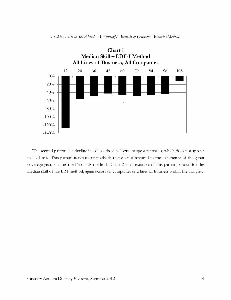
Looking Back to See Ahead: A Hindsight Analysis of Common Actuarial Methods
Casualty Actuarial Society E-Forum, Summer 2012 4
The second pattern is a decline in skill as the development age d increases, which does not appear to level off. This pattern is typical of methods that do not respond to the experience of the given coverage year, such as the FS or LR method. Chart 2 is an example of this pattern, shown for the median skill of the LR1 method, again across all companies and lines of business within the analysis.
-140%
-120%
-100%
-80%
-60%
-40%
-20%
0%12 24 36 48 60 72 84 96 108
Chart 1Median Skill – LDF-I Method
All Lines of Business, All Companies
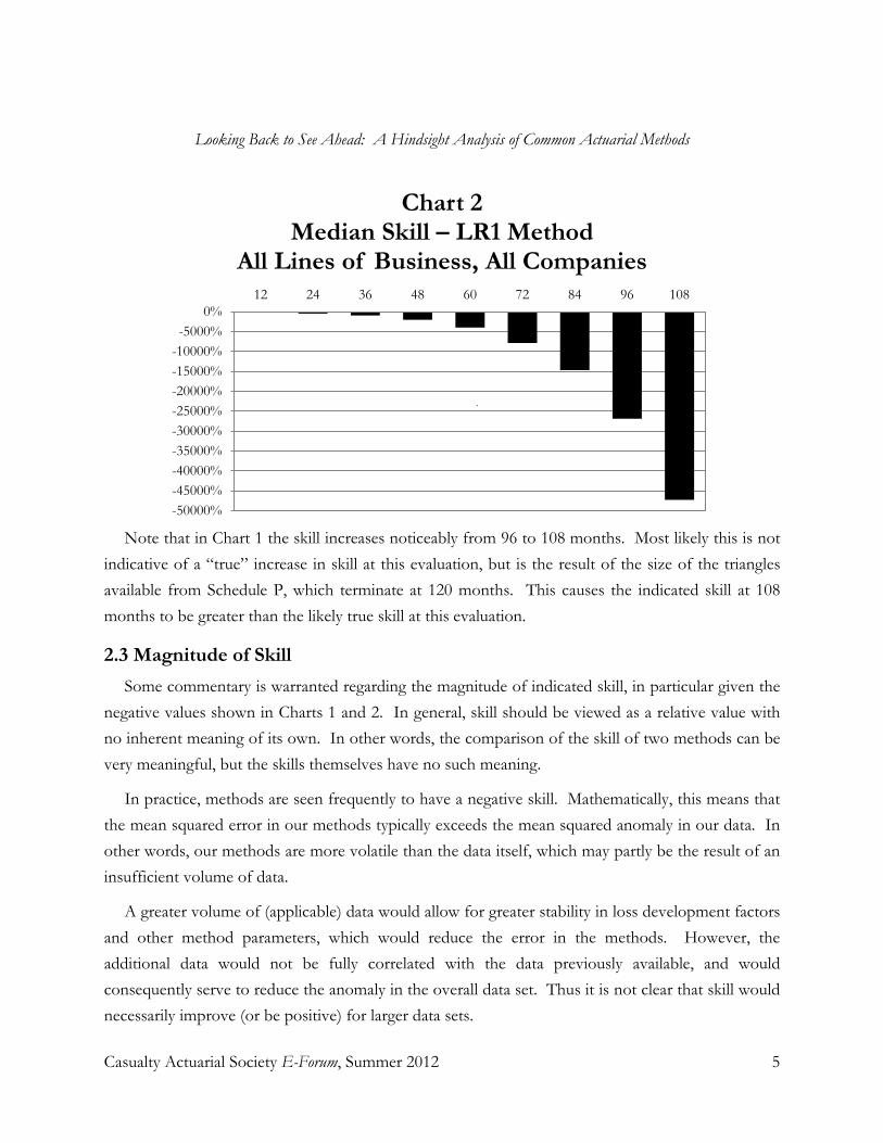
Looking Back to See Ahead: A Hindsight Analysis of Common Actuarial Methods
Casualty Actuarial Society E-Forum, Summer 2012 5
Note that in Chart 1 the skill increases noticeably from 96 to 108 months. Most likely this is not
indicative of a “true” increase in skill at this evaluation, but is the result of the size of the triangles available from Schedule P, which terminate at 120 months. This causes the indicated skill at 108 months to be greater than the likely true skill at this evaluation.
2.3 Magnitude of Skill Some commentary is warranted regarding the magnitude of indicated skill, in particular given the
negative values shown in Charts 1 and 2. In general, skill should be viewed as a relative value with no inherent meaning of its own. In other words, the comparison of the skill of two methods can be very meaningful, but the skills themselves have no such meaning.
In practice, methods are seen frequently to have a negative skill. Mathematically, this means that the mean squared error in our methods typically exceeds the mean squared anomaly in our data. In other words, our methods are more volatile than the data itself, which may partly be the result of an insufficient volume of data.
A greater volume of (applicable) data would allow for greater stability in loss development factors and other method parameters, which would reduce the error in the methods. However, the additional data would not be fully correlated with the data previously available, and would consequently serve to reduce the anomaly in the overall data set. Thus it is not clear that skill would necessarily improve (or be positive) for larger data sets.
-50000%-45000%-40000%-35000%-30000%-25000%-20000%-15000%-10000%-5000%
0%12 24 36 48 60 72 84 96 108
Chart 2Median Skill – LR1 Method
All Lines of Business, All Companies
Looking Back to See Ahead: A Hindsight Analysis of Common Actuarial Methods
Casualty Actuarial Society E-Forum, Summer 2012 6
Additional insight can be gained by observing that the concept of skill originates in meteorology4
We may assume that the meteorological method described above has 0% skill because the new information provided by tomorrow’s high temperature will have very little impact on the calculation of the mean squared anomaly. This is strongly in contrast to a typical reserving scenario, in which estimates of development factors and loss ratios, to take two examples, often change significantly with the introduction of one new data valuation. Consequently, because the true anomaly of our data sets remains unknown, actuarial reserving methods will often exhibit negative skill.
. It seems reasonable that if we were to estimate tomorrow’s high temperature as the average of the historical high temperatures for the same date, such a method might have a skill of 0%, with an expected mean squared error equal to the historical mean squared anomaly in the temperatures. Consequently a method that incorporates additional information, such as today’s high temperature, into the prediction of tomorrow’s high temperature would presumably represent an improvement and thus have positive skill.
2.4 How to Interpret an Improvement in Skill It is helpful to have an intuitive understanding of skill and, in particular, what an increase in skill
means regarding the volatility of a given method. As an example of this, consider as hypothetical examples Companies A, B, and C. These companies each write different volumes of what are otherwise similar books of business.
At a given month of development, Companies A, B, and C each have an expected unpaid loss ratio (i.e., unpaid loss relative to earned premium for the given coverage year) of 10%. Company A writes the most business, and Company A’s data therefore exhibits the least variation. Company C writes the least business, and its data therefore exhibits the most variation. The mean squared anomalies of Companies A, B, and C’s data at the given month of development are given in Table 2. This represents a fairly common range of mean squared anomalies when the expected unpaid loss ratio is approximately 10%.
4 Additional discussion regarding the origins of skill can be found in [8].

Looking Back to See Ahead: A Hindsight Analysis of Common Actuarial Methods
Casualty Actuarial Society E-Forum, Summer 2012 7
TABLE 2 MEAN SQUARED ANOMALY – HYPOTHETICAL EXAMPLES
Company Mean Squared Anomaly
A 0.1%
B 0.4%
C 1.6%
With this information we can calculate the impact of an increase in skill for a given method on the expected error in the unpaid loss, relative to the expected unpaid loss itself. The percentages in Table 3 are calculated algebraically based on the formula for skill. The square root of the mean squared error (RMSE) as a percent of unpaid loss is then equal to the RMSE as a percent of premium divided by the unpaid loss ratio.
TABLE 3 COMPANY A: CHANGE IN MEAN ABSOLUTE ERROR RELATIVE TO
UNPAID LOSS, GIVEN A CHANGE IN SKILL Skill Mean Squared
Error RMSE* as a Percent of Premium
RMSE* as a Percent of Unpaid
Loss
1% 0.00% 0.3% 3.2%
2 0.00 0.4 4.5
5 0.01 0.7 7.1
10 0.01 1.0 10.0
15 0.02 1.2 12.2
20 0.02 1.4 14.1
30 0.03 1.7 17.3
50 0.05 2.2 22.4
* Square root of the mean squared error.

Looking Back to See Ahead: A Hindsight Analysis of Common Actuarial Methods
Casualty Actuarial Society E-Forum, Summer 2012 8
When expressed in this manner the impact of a change in skill becomes more apparent. For example, if we were able to improve the skill of an actuarial analysis for Company A by 50%, the RMSE within such an analysis would decline by approximately 22%, relative to the unpaid loss. The relationship between a change in skill for Companies A, B and C is shown in Chart 3. Thus for Companies B and C, whose books of business exhibit greater variation than Company A’s, the reduction in RMSE is proportionally greater for the same change in skill than is the case for Company A. This implies, in a practical sense, that method skill becomes more important as the data becomes thinner.
0.0%
10.0%
20.0%
30.0%
40.0%
50.0%
60.0%
70.0%
80.0%
90.0%
100.0%
0% 2% 4% 6% 8% 10%
12%
14%
16%
18%
20%
22%
24%
26%
28%
30%
32%
34%
36%
38%
40%
42%
44%
46%
48%
50%
Change in Skill
Chart 3Change in Square Root of the Mean Squared Error
As a Percent of Unpaid Loss
Company A
Company B
Company C

Looking Back to See Ahead: A Hindsight Analysis of Common Actuarial Methods
Casualty Actuarial Society E-Forum, Summer 2012 9
3. DISCUSSION OF RESULTS
The best-performing methods (i.e., the methods with the greatest skill) in the analysis were observed to satisfy the following two criteria:
1. Each relies at least in part on case reserves (“Criterion 1”).
2. Amounts paid to date do not directly influence the indicated unpaid loss (“Criterion 2”).
As a general example of this, consider Chart 4, which compares three common loss development methods, the LDF-I, LDF-P, and CDF methods. Results are shown across all companies and lines of business.
Thus the skill of the LDF-I method is seen clearly to exceed that of the LDF-P method. Results
for the LDF-I method and CDF method are similar at earlier evaluations, although beginning at the 84-month evaluation the CDF method outperforms the LDF-I method. Differences in skill for the LDF-P and LDF-I methods exceed 100% at the first evaluation but remain close to or above 60% at later evaluations.
However, there are various methods that meet Criterion 1 and Criterion 2, and the CDF method is not necessarily the best of these. Consider the comparison given in Chart 5 across most of the methods that meet these characteristics. Of the five methods shown, the BF1-I method appears somewhat superior to the other methods considered. However, for any given company, this will
-300%
-250%
-200%
-150%
-100%
-50%
0%12 24 36 48 60 72 84 96 108
Chart 4LDF-I, LDF-P and CDF Methods
Median Skill, All Companies, All Lines of Business
LDF-I LDF-P CDF

Looking Back to See Ahead: A Hindsight Analysis of Common Actuarial Methods
Casualty Actuarial Society E-Forum, Summer 2012 10
depend on the applicability (more accurately, the skill) of the a priori loss ratio indications available.
It should be noted that the BT-I, BF2-I, CC-I, and IM-I methods are excluded from the above chart due to space constraints, although they each satisfy Criteria 1 and 2. The IM-I method significantly underperformed the other methods considered. Presumably this is due to the leveraged nature of the parameters on which this method relies. The other three methods on this list each underperformed the methods included in Chart 5, but only somewhat.
-300%
-250%
-200%
-150%
-100%
-50%
0%12 24 36 48 60
Chart 5Methods Satisfying Criteria 1 and 2
Median Skill, All Companies, All Lines of Business
CDF BF1-I IA-I BRC HS-I

Looking Back to See Ahead: A Hindsight Analysis of Common Actuarial Methods
Casualty Actuarial Society E-Forum, Summer 2012 11
A similar comparison of the LDF-I method is made in Chart 6 with other methods that possess
Criterion 1 but not Criterion 2. The LDF-I method is seen in Chart 6 to outperform the other incurred-based methods. At the earliest two evaluations, the BLS-I method outperforms the other incurred-based methods considered. However, the BLS-I method becomes too leveraged at later evaluations (beginning at 36 months) and underperforms the MCL-I and BS methods at this point.
The paid-based methods can be similarly compared, which shows that these methods generally underperform the LDF-P method. The paid-based methods that outperform the LDF-P method are the BF1-P, BT-P, and HS-P methods. However, these methods underperform the LDF-I method.5
3.1 Results by Company Size
Note that these three methods satisfy Criterion 2 but not Criterion 1 (the remainder of the paid-based methods considered do not satisfy either of the criteria). Thus we could conclude that, while both criteria are important to method skill, Criterion 1 is more important than Criterion 2.
Results were similarly considered by company size, in which each company was segregated into a “Small,” “Medium,” or “Large” category. Companies were not permitted to migrate segments between evaluations, and were segregated according to their average annual net earned premium
5 All three methods underperformed the LDF-I method at 24 months of development and subsequent. At 12 months of development, the BF1-P and BT-P methods outperformed the LDF-I method, while the HS-P method did not.
-250%
-200%
-150%
-100%
-50%
0%12 24 36 48 60
Chart 6Incurred-Based Methods
Median Skill, All Companies, All Lines of Business
LDF-I MCL-I BS BLS-I

Looking Back to See Ahead: A Hindsight Analysis of Common Actuarial Methods
Casualty Actuarial Society E-Forum, Summer 2012 12
across all years considered. Table 4 provides the average 2010 net earned premium for the companies in each category.
TABLE 4 AVERAGE 2010 NET EARNED PREMIUM BY CATEGORY
Company Size Average 2010 Net Earned Premium
Small $4.2 million
Medium $17.5 million
Large $350.0 million
In general, Criterion 2 was seen to be more important for small companies and less important for large companies, relative to all companies considered as a whole. In other words, for small companies, methods in which paid loss directly influences unpaid loss (e.g., the LDF-I method) are seen to have less skill, relative to other methods, than was the case when considering all companies as a whole. For large companies, methods such as the LDF-I method perform as well as methods such as the CDF method, and in some cases outperform these methods.
However, the general relationship between the various methods satisfying Criteria 1 and 2 that was present for all companies appears to hold when large companies are considered on their own. This is seen in Chart 7. Note that results in Chart 7 are shown through 36 months and that results subsequent to 36 months are similar.
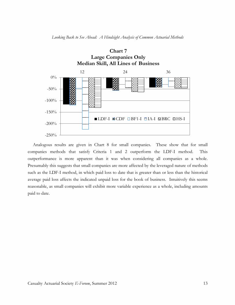
Looking Back to See Ahead: A Hindsight Analysis of Common Actuarial Methods
Casualty Actuarial Society E-Forum, Summer 2012 13
Analogous results are given in Chart 8 for small companies. These show that for small
companies methods that satisfy Criteria 1 and 2 outperform the LDF-I method. This outperformance is more apparent than it was when considering all companies as a whole. Presumably this suggests that small companies are more affected by the leveraged nature of methods such as the LDF-I method, in which paid loss to date that is greater than or less than the historical average paid loss affects the indicated unpaid loss for the book of business. Intuitively this seems reasonable, as small companies will exhibit more variable experience as a whole, including amounts paid to date.
-250%
-200%
-150%
-100%
-50%
0%12 24 36
Chart 7Large Companies Only
Median Skill, All Lines of Business
LDF-I CDF BF1-I IA-I BRC HS-I

Looking Back to See Ahead: A Hindsight Analysis of Common Actuarial Methods
Casualty Actuarial Society E-Forum, Summer 2012 14
3.2 Results by Line of Business Results were also considered by line of business, where line of business was defined by the
segments used within Schedule P. In general the results discussed above did not vary significantly by line of business. However, there are two apparent exceptions to this observation, specifically for the Homeowners and Workers Compensation lines of business.
Chart 9 displays the observed results for Homeowners coverage. In general the directional relationships between the methods are similar as when all lines are considered in tandem. However, the relative performance of the CDF method as compared to the LDF-I method is clearly different, with the CDF method outperforming the LDF-I method (as well as the LDF-P method). This may be the result of the fast-paying nature of Homeowners coverage for most claims.
When all lines of business were considered together, we saw that at later months of development (in particular, at 84 months of development and subsequent) the CDF method outperformed the LDF-I method. At this evaluation, the majority of claims are paid for most lines of business. For the Homeowners line of business, this point in time (when the majority of claims are paid) is reached much earlier. In general, it appears that the CDF method and other methods satisfying Criteria 1 and 2 may be most useful at “later” evaluations (where the definition of “later” varies by line of business according to the rate of payments).
-400%-350%-300%-250%-200%-150%-100%-50%
0%12 24 36
Chart 8Small Companies Only
Median Skill, All Lines of Business
LDF-I CDF BF1-I IA-I BRC HS-I

Looking Back to See Ahead: A Hindsight Analysis of Common Actuarial Methods
Casualty Actuarial Society E-Forum, Summer 2012 15
Chart 10 demonstrates a very different situation for Workers Compensation. For this line of
business, the LDF-I method clearly outperforms the CDF method. Two possible reasons exist for this observation. The first is that the rate of payment for Workers Compensation claims is slower than for property & casualty coverages considered as a whole, and certainly slower than for Homeowners claims. This suggests a reason analogous to that observed for Homeowners, and that at a “later” evaluation the CDF method would outperform the LDF-I method for Workers Compensation. (This “later” evaluation would requisitely be at some point past 108 months, as the LDF-I method outperforms the CDF method for Workers Compensation at all evaluations made available by the Schedule P data.)
-120%
-100%
-80%
-60%
-40%
-20%
0%12 24 36 48 60
Chart 9Homeowners Line of Business
Median Skill, All Companies
LDF-I LDF-P CDF BF1-I

Looking Back to See Ahead: A Hindsight Analysis of Common Actuarial Methods
Casualty Actuarial Society E-Forum, Summer 2012 16
The second reason is the regular pattern of payments exhibited by Workers Compensation
claims, as this rate of payments is largely determined by legislation. For most other lines of business, the rate of payments can be raised by efforts to settle claims more quickly, and the observed rate of payments can be altered by a particular large claim. Workers Compensation payments are largely immune to this phenomenon, as even a claim with a large medical component will often exhibit a rate of payments similar to other claims. Consequently the disadvantage of the LDF-I method that was observed earlier – that this method is easily biased up or down by the presence of absence of a large claim or larger than usual number of paid claims – does not apply to Workers Compensation.
While the number of claims with amounts paid to date for Workers Compensation in a particular coverage year may be greater or lesser than average, the paid loss on these claims is predictive of unpaid loss. Any Workers Compensation claim open 12 months after its accident date is generally a claim on which payments have been made to date and on which payments will be made for several years into the future (and perhaps for the lifetime of the claimant). Similarly, any Workers Compensation claim closed within this timeframe will generally have had a relatively small amount of payments (relative to the claims remaining open), making the impact of paid loss on such claims on unpaid loss within the LDF-I method largely immaterial. While the larger paid loss on claims remaining open would impact the indication of unpaid loss, these paid amounts, separated by an accounting date, would be reasonably expected to be highly correlated. Thus, under this reasoning, the CDF method is not necessarily a “worse” method for Workers Compensation, but the LDF-I
-180%-160%-140%-120%-100%-80%-60%-40%-20%
0%12 24 36 48 60
Chart 10Workers Compensation Line of Business
Median Skill, All Companies
LDF-I LDF-P CDF BF1-I

Looking Back to See Ahead: A Hindsight Analysis of Common Actuarial Methods
Casualty Actuarial Society E-Forum, Summer 2012 17
method is a relatively “better” method, when compared to its performance for other lines of business.
This reasoning begs the question as to why the LDF-P method underperforms for the Workers Compensation line of business, similar to its performance for other lines. It is possible that if a much larger triangle of payments were available for Workers Compensation, the LDF-P method would not underperform, and might even outperform the LDF-I method. As discussed in Appendix A, to develop paid loss to the same level as incurred loss, it is necessary within the LDF-P method to apply a ratio of incurred-to-paid loss to the paid loss developed to a 10th report.
The ratio of paid-to-incurred loss will typically be greater than the ratio that is applied for other lines of business, and will typically be subject to greater volatility than for other lines of business. This ratio would not be necessary in the more common reserving scenario in which a larger triangle of paid Workers Compensation loss was available. Consequently, particular caution should be taken in inferring the applicability of these results for Workers Compensation onto the skill of methods in a reserve analysis for which a greater history of paid loss data is available.
4. EFFECT OF CORRELATION
An interesting observation can be made in comparing the skill of three methods highlighted previously: the LDF-I, LR1, and BF1-I methods. Chart 11 shows the skill of these three methods on a logarithmic scale6
Recall that the BF1-I method is a weighted average of the LDF-I methods and LR1 methods, in which the weights are determined by the loss development factors of the LDF-I method. Yet the skill of the BF1-I method is clearly greater than the skill of either of the two methods of which it is comprised. This is the result of correlation, and in particular the observation that the LR1 and LDF-I methods are partially but not fully correlated. Consequently the BF1-I method takes more
. A logarithmic scale was used due to the vast disparity between the skill of the LR1 method and the other two methods (see Chart 2 and prior discussion concerning the LR1 method, and note that despite the logarithmic scale the skill of the LR1 appears within the range of the chart for only the first two evaluations).
6 More precisely, the translation used given a median skill of S to a logarithmic (median) skill of L was L = – Ln [– (S – 1)]. Thus, since S must be less than or equal to 1, L was well-defined for all values of S. Negating the value of the logarithm ensures that L will exhibit the same property as S, in that if the skill of a given method is greater than another, its logarithmic skill will be greater as well.

Looking Back to See Ahead: A Hindsight Analysis of Common Actuarial Methods
Casualty Actuarial Society E-Forum, Summer 2012 18
information into account than either of these methods on their own, and the weighting of these two methods is such that the resulting observed skill is greater.
This observation holds for any method calculated as the weighted average of other methods. As
additional examples, consider Charts 12 and 13. The first of these charts compares the skill of the LDF-I and LDF-P methods with a new method for estimating unpaid loss calculated as 90% of the unpaid loss indication from the LDF-I method and 10% of the unpaid loss indication from the LDF-P method. For earlier evaluations, this new method performs comparably to the LDF-I method. For later evaluations (beginning at 60 months, as shown in Chart 12), the new method represents an improvement in skill. (Note that a 50/50 weighting of the LDF-I and LDF-P methods produced a method that underperforms relative to the LDF-I method.)
-300%
-250%
-200%
-150%
-100%
-50%
0%36 48 60 72 84
Chart 11Logarithmic Skill
All Companies, All Lines of Business
LDF-I LR1 BF1-I

Looking Back to See Ahead: A Hindsight Analysis of Common Actuarial Methods
Casualty Actuarial Society E-Forum, Summer 2012 19
Chart 13 similarly shows the skill of four methods, the LDF-I and HS-I methods, a 50/50
weighting of these two methods, and a 90/10 weighting of these two methods (in which 90% of the weight is given to the HS-I method). It is easily seen that each of the weighted average methods outperform the two component methods (results before 36 months and after 84 months are similar to these respective observations). This suggests that the use of multiple methods (provided they are properly chosen) is very important to the skill of any actuarial analysis. The LDF-I and HS-I methods are two of the best-performing methods from the analysis, yet we are easily able to improve on the skill of these methods with a straight average of the two, and able to improve even more by judgmentally refining the weights.
-120%
-100%
-80%
-60%
-40%
-20%
0%
20%60 72 84 96 108
Chart 12Weighted Average of the LDF-I and LDF-P MethodsMedian Skill, All Companies, All Lines of Business
LDF-I LDF-P 90% LDF-I / 10% LDF-P

Looking Back to See Ahead: A Hindsight Analysis of Common Actuarial Methods
Casualty Actuarial Society E-Forum, Summer 2012 20
5. APPROACH TO ANALYSIS
Some discussion regarding the selection of method skill as the appropriate metric for the current analysis is warranted. Various techniques have been suggested for use in evaluating the hindsight performance of actuarial methods. These have historically fallen in three categories:
1. “The Scorecard System” compares the indicated ultimate loss for an individual entity or data set, where the comparison is made either from one evaluation to the next or from a given evaluation to the “true ultimate” loss, once that is known. References [10] and [16] are both examples of this technique. An advantage of this technique is its simplicity and ease of explanation, but a disadvantage is that it provides no way of aggregating observed results for a single method or entity, or across multiple methods or entities. For this reason the technique has typically been used for single entities or data sets only.
2. Calculating the mean and standard deviation of the prediction errors, and similar statistical calculations related to the prediction error’s distribution, is another evaluation
-60%
-50%
-40%
-30%
-20%
-10%
0%36 48 60 72 84
Chart 13Weighted Average of the LDF-I and HS-I MethodsMedian Skill, All Companies, All Lines of Business
LDF-I HS-I 50% HS-I / 50% LDF-I 90% HS-I / 10% LDF-I

Looking Back to See Ahead: A Hindsight Analysis of Common Actuarial Methods
Casualty Actuarial Society E-Forum, Summer 2012 21
method. Here, prediction error is defined as the difference between true ultimate loss and the ultimate loss indicated by a given method as of a given evaluation. References [3], [12], [13], and [15] are examples of this technique. In each of these monographs, triangular data sets are simulated under a set of assumptions and standard actuarial methods are applied to the simulated data in a mechanical fashion. Hence, given the underlying assumptions, the distribution of prediction error is readily known, provided that a sufficient number of triangular data sets are simulated.
The assumptions used in the simulation are typically specific to a given line of business or amount of business written, however, and consequently the results may not be applicable to other lines of business or situations when a greater or lesser amount of business is written. For example, claims may be assumed to be reported promptly after occurrence, or it may be assumed that there is a significant lag in claim reporting, and both assumptions can have a significant impact on the performance of claim-based methods. Similarly, the amount of business written will clearly impact the standard deviation of prediction error, and some methods may be impacted more than others.
For the analysis considered here, multiple lines of business were analyzed across various company sizes. Consequently any attempt to derive statistics concerning the distribution of prediction error would either need to consider each line of business and company size grouping separately, or would need to attempt to normalize for these differences. Even if data were segregated, differences in company size would still exist between different companies in the group, and any attempt at additional segmentation to mitigate this issue would likely result in a statistically insignificant sample size. Any attempt at normalization across companies or lines of business would ideally consider the amount of business written as well as the inherent volatility of that business.
3. Method skill has the advantage of normalizing for differences in premium earned and the resulting volatility in unpaid loss by company (a disadvantage in the discussion of the distribution of prediction error above). Taking the form of a single numeric value can be seen as both an advantage and a disadvantage. Method skill will not provide additional information on the distribution of prediction error, and in particular will not indicate whether a method is biased. Taking the form of a single numeric value, however, allows more easily for comparison across different companies and lines of business.
One final aspect of method skill that should be considered is that, by itself, it

Looking Back to See Ahead: A Hindsight Analysis of Common Actuarial Methods
Casualty Actuarial Society E-Forum, Summer 2012 22
provides no statistical significance of its indication. Observations regarding statistical significance could be added to an analysis such as this by segregating data triangles randomly into two or three groups, then comparing the indicated skill for each group. While this random segmentation is outside the scope of the current analysis, segmentation of results has been done by company size and line of business, as discussed above. The general similarity of results by line of business (with the exception of the Homeowners and Workers Compensation lines) suggests a meaningful level of statistical significance for the results, although this cannot be measured with precision.
6. CONCLUSIONS
The results of this empirical analysis suggest three conclusions:
A. In most situations, the methods with greatest skill are those satisfying Criteria 1 and 2, first defined in Section 3 above:
1. Each relies at least in part on case reserves (“Criterion 1”).
2. Amounts paid to date do not directly influence the indicated unpaid loss (“Criterion 2”).
B. These methods (those possessing the greatest skill) are not commonly in use.
C. The weighting schemes most commonly in use are not supported by the current analysis.
Consider that the LDF-I and LDF-P methods are ubiquitous throughout reserve analyses. While the best reserve analyses will almost always contain other methods as well, significant weight is typically given to these two methods. However the above results suggest that many more valuable methods exist, and that the LDF-P method in particular should receive little to no weight in most analyses. This is noticeably in contrast to the 50/50 weighting used in many reserve analyses for the LDF-I and LDF-P methods.
Where not already in use, we could greatly improve our analyses by use of methods satisfying Criteria 1 and 2. In particular, the CDF, IA-I, BR, and HS-I methods would all serve in many cases to enhance and improve our work. Various versions of the BF method are commonly in use now, although this analysis suggests that greater weight should likely be given to the BF methods than is typical currently. Often BF methods are viewed as appropriate for “middle” years, yet the current analysis suggests that giving weight to the BF methods can improve our analyses for all years.

Looking Back to See Ahead: A Hindsight Analysis of Common Actuarial Methods
Casualty Actuarial Society E-Forum, Summer 2012 23
Additional work in the area of method weights would be helpful, as this paper has merely touched the surface of that topic. Results shared here suggest that the selection of method weights is significant to the skill of an analysis, perhaps more so than the methods themselves. Consider, for example, that little improvement in skill is gained by switching from the LDF-I method to the HS-I method. However, a 25% additive improvement in skill is gained at all evaluations by using a 90/10 weighted average of the HS-I and LDF-I methods, respectively.
Another topic not addressed here is the weighting of more than two methods, as would be done in practice. It is likely that as any method is added to an analysis already consisting of several methods, the incremental skill achieved by giving weight to such a method will decline as the number of methods already incorporated into the weighted average increases. However, the number of methods required before this incremental skill becomes minimal is an open question, as is whether this number could be reduced by appropriate selection and weighting of the methods. Additional research in this area is welcome.
Acknowledgment
The author would very much like to thank: • For their many hours programming the analysis discussed here, Paul Keuler, Linda Gritter, and Shaun
Cullinane (who also provided helpful comments on the paper itself); • For assistance with graphs as well as the underlying analysis, Brooke Mote-Nirode; and • For comments and review of the analysis itself, Eric Wunder, Mark Mulvaney, and Jeff Courchene.

Looking Back to See Ahead: A Hindsight Analysis of Common Actuarial Methods
Casualty Actuarial Society E-Forum, Summer 2012 24
Appendix A – Loss Reserving Methods The following provides a list of the methods considered in the analysis, including the
abbreviation used to refer to each method (note that for methods for which there are paid and incurred versions, multiple abbreviations are given). Also included is any relevant information as to how the method is applied within the current analysis, given the data limitations of Schedule P. As discussed further in Appendix B, the methods outlined below develop indications of loss at a 10th report (i.e., the last evaluation included within the Schedule P triangles) rather than indications of loss at ultimate.
1. Backward Recursive Case Development (BRC)
This method is discussed by Marker and Mohl in [11]. The paid-on-prior-case and case-on-prior-case factors selected for our analysis are each the weighted average of the columns of these factors as given by the triangles, where the weights are proportional to the prior case. At a 10th report, we have assumed a paid-on-prior-case factor of 1.00 and a case-on-prior-case factor of 0.00.
2. Benktander (BT)
The Benktander method, discussed in [9], is often referred to as the “iterated Bornhuetter-Ferguson method.” In the BT method, a priori loss is equal to the indication from the BF method (in our case, BF1-I for the incurred method, and BF1-P for the paid method). The calculation of indicated loss then proceeds as described for the BF method, with calculations of the percent unpaid for the BT-P method and the percent IBNR for the BT-I method.
3. Berquist-Sherman Case Adjustment (BS)
The BS method is the first of the two methods given in [2], in which an adjustment is made to the incurred loss in the prior diagonals of a given triangle for assumed changes in case reserve adequacy. This adjustment is made by de-trending the average case reserve along the most recent diagonal of the triangle (in the case of the current analysis, at a rate of 5.0% per annum). The result is multiplied by the number of open claims within prior diagonals in order to obtain an indication of case reserves from prior diagonals at the approximate level of case reserve adequacy as the most recent diagonal. Incurred loss development factors are then developed and applied to loss along the most recent diagonal as for the LDF-I method.
4. Bornhuetter-Ferguson 1 (BF1)
The first of the BF methods included in the analysis uses the indicated loss from the first loss ratio method (LR1), described below, as the a priori indicated loss. The percent unpaid and percent IBNR are then calculated as described in [4], producing both paid (BF1-P) and incurred (BF1-I) versions of this method.

Looking Back to See Ahead: A Hindsight Analysis of Common Actuarial Methods
Casualty Actuarial Society E-Forum, Summer 2012 25
5. Bornhuetter-Ferguson 2 (BF2)
The second of the BF methods is an iterative procedure in which the a priori indicated loss is based on the weighted average loss ratios of preceding accident years, as based on the BF2 method indications for these years. The oldest accident year in the triangle, as well as any other accident year for which loss ratios of older accident years are not available, relies on the same a priori loss ratio as the BF1 method. Both paid (BF2-P) and incurred (BF2-I) versions of this method are calculated.
6. Brosius Least Squares (BLS)
The BLS method considers that there may be both additive and multiplicative aspects of loss development. Thus the method iteratively develops both a multiplicative loss development factor, to be applied to losses paid or incurred to date, and an additive factor, to be included subsequent to the multiplication. The factors are based on a least squares regression, where the incurred loss ratio at a 10th report is the dependent variable and the paid or incurred loss ratio at the given evaluation is the independent variable. The use of loss ratios rather than loss is a difference from the methodology as presented in [5], and was done so as to normalize for changes in exposure across accident years. Both paid (BLS-P) and incurred (BLS-I) versions are included.
7. Brosius Least Squares – Weighted (BLSW)
Having observed certain indications produced by the BLS method, we sought to enhance the reliability of this method by giving more credibility in the regression process to years with greater premium, and presumably greater exposure. The Weighted Brosius Least Squares method that resulted uses a regression process weighted by premium, in contrast to the unweighted regression used in the BLS method itself.
8. Cape Cod (CC)
The Cape Cod method is very similar to the BF method, but develops a priori loss under the assumption that in total across accident years it should be equal to the CC method indication. For the CC method as included in this analysis, we have assumed the same loss ratio for each accident year (i.e., unlike certain of the loss ratio methods discussed below, there is no a priori difference assumed by year). Both paid (CC-P) and incurred (CC-I) versions of the method are included.
9. Case Development Factor (CDF)
The CDF method is based on the loss development factors from the LDF method, discussed below. In the CDF method an indicated unpaid-to-case ratio is derived from the relationship between unpaid loss and case loss implicit in the selected paid and incurred loss development

Looking Back to See Ahead: A Hindsight Analysis of Common Actuarial Methods
Casualty Actuarial Society E-Forum, Summer 2012 26
factors. This factor is then applied to the case reserve to derive an indication of unpaid loss, which is added to paid loss to date for an indication of loss incurred through the 10th report.
10. Frequency/Severity (FS)
The FS method is based on a projection of reported claims at a 10th report and a severity applied to these claims. Reported claims are based on the company’s triangular reported claims data (i.e., Section 3 of Part 5 of Schedule P for the given line of business) developed to a 10th report using weighted average reported claim development factors. Given the relatively favorable performance of the LDF-I method as well as its general acceptance within actuarial practice, we took the LDF-I method to be the “preliminary” selected method for use in selecting severities. Thus the severity for each accident year is calculated as the incurred loss at a 10th report indicated by the LDF-I method divided by the indicated reported claims at a 10th report. For a given accident year, a severity is selected based on the weighted average severities of all prior accident years, where the weights are proportional to the projected reported claims. In this process, the severities are trended to the accident year in question at a rate of 5.0% per annum.
11. Hindsight Outstanding/IBNR (HS)
The HS method is similar to the FS method in that it relies on an equivalent projection of reported claims as well as a preliminary selected loss method (also the LDF-I method). However within the HS method, the projection of reported claims is used to calculate a triangle of “hindsight outstanding” claims, which are the difference between the projection of reported claims at a 10th report and closed claims to date. Similarly, the preliminary selected loss method is used to calculate a triangle of hindsight outstanding loss, which is the difference between the preliminary method loss projections and the paid or incurred loss to date. Thus the difference represents unpaid loss for the HS-P method and IBNR loss for the HS-I method. The ratios of the values within the hindsight outstanding loss triangle to the corresponding values within the hindsight outstanding claims triangle produces a triangle of hindsight outstanding severities (unpaid severities for the HS-P method and IBNR severities for the HS-I method). For a given accident year, severities from the preceding years are trended at 5.0% per annum to the accident year in question. A weighted average of these severities, where the weights are proportional to hindsight outstanding claims, is selected. The weighted average hindsight severity is then applied to the number of projected outstanding claims for the given accident year to produce indications of unpaid loss for the HS-P method and IBNR loss for the HS-I method. These are then added to paid loss or incurred loss, respectively, to derive indications of incurred loss at a 10th report. This method is also referred to as the “ultimate unclosed claim severity technique” within [7].

Looking Back to See Ahead: A Hindsight Analysis of Common Actuarial Methods
Casualty Actuarial Society E-Forum, Summer 2012 27
12. Incremental Additive (IA)
In this method, incremental (i.e., calendar year) changes in paid or incurred loss are observed by accident year and compared to the premium for that year. A weighted average ratio of incremental loss to premium is selected, where the weights are proportional to the premium. These ratios are accumulated to derive an IBNR-to-premium or unpaid-to-premium ratio at the given evaluation. The ratios are applied to premium to derive IBNR or unpaid loss itself, then added to incurred loss or paid loss, respectively, for the IA-I and IA-P methods. So that the IA-P method will produce an indication of incurred loss at a 10th report, the unpaid-to-premium ratio at a 10th report is set equal to the case-to-premium ratio at a 10th report of the earliest year in the triangle.
13. Incremental Claims Closure (ICC)
The incremental claims closure method is described by Adler and Kline in [1]. In this method, reported claims at a 10th report are projected based on the reported claims triangle and weighted average reported claims development factors selected from this triangle (as above for the FS and HS methods). A closing pattern is then selected based on historical weighted average incremental closed-on-prior-open factors, where the weights are proportional to the number of claims open. These factors are then applied iteratively to project incremental closed claims, with the difference between the projected reported claims at the 10th report and the projected closed claims at the 10th report being the number of claims projected to close after the 10th report. As the next step, historical incremental paid loss is compared to incremental closed claims to derive incremental paid loss per closed claim by time period. These amounts are then trended at 5.0% per annum to the relevant time period and a weighted average of the indications selected (where the weights are proportional to the number of closed claims). Prospective incremental paid loss by accident year is then projected as the product of the projected incremental closed claims and the projected paid loss per closed claim, each for the same time period. Ultimate loss is then the sum of these projections with paid loss to date. Within the current analysis, claims that are projected to close after the 10th report are assumed to have a severity equal to that of the claims that close between the 9th and 10th reports, but trended one additional year.
14. Incremental Multiplicative (IM)
The incremental multiplicative method is similar to the incremental additive method in that both methods consider incremental loss triangles. However, the IM method calculates development factors that are ratios of incremental loss in one time period to the incremental loss in the preceding time period. Weighted averages of these development factors are calculated, where the weights are proportional to the incremental loss in the preceding time period. The development factors are then applied iteratively to project incremental loss in subsequent time periods. Projections of unpaid loss and IBNR loss are derived for the IM-P and IM-I methods, respectively, by accumulating the indications of incremental paid and incremental

Looking Back to See Ahead: A Hindsight Analysis of Common Actuarial Methods
Casualty Actuarial Society E-Forum, Summer 2012 28
incurred loss by time period. These projections of unpaid loss and IBNR loss are added to paid loss to date and incurred loss to date, respectively, to derive distinct indications of ultimate loss. Within the IM-P method, a tail factor from paid loss at a 10th report to a level reflecting incurred loss at a 10th report is selected based on the oldest accident year in the triangle and the assumption that the case loss within this accident year will be paid as is. In other words, the tail factor is the case loss for this year divided by the incremental paid loss for this year in the time period preceding the 10th report. If incremental paid loss for this time period is zero, then such a ratio is undefined and assumed to be zero for purposes of our analysis.
15. Loss Development Factor (LDF)
The LDF methods are based on the calculation of historical loss development factors from the paid and incurred triangles. The weighted average loss development factor from all available years within the triangle is applied to loss at the given evaluation date to derive indicated loss at a 10th report. Both paid (LDF-P) and incurred (LDF-I) versions of this method are included within the analysis. For the paid method, a tail factor to develop the losses from paid at a 10th report to incurred at a 10th report is equal to the incurred-to-paid ratio at a 10th report for the earliest year in the triangle.
16. Loss Ratio – Based on A Priori Assumption (LR1)
Three versions of the loss ratio method are included within our analysis. Each relies on net earned premium by calendar year, consistent with the use of net paid and incurred loss within the triangles. The first of these (LR1) is based on a priori industry indications of the loss ratio for the given coverage year. These loss ratios were derived from historical A.M. Best Review & Preview reports.
17. Loss Ratio – Based on Preliminary Selected for Prior Years (LR2)
The remaining two loss ratio methods are each based on the use of preliminary selected incurred loss at a 10th report, which for both is set equal to the results of the LDF-I method, consistent with the preliminary selected loss in the FS and HS methods. For the LR2 method, the loss ratio for a given accident year is set equal to the weighted average of the loss ratios produced by the preliminary selected method within the preceding accident years of the triangle, where the weights are proportional to net earned premium. This loss ratio is then multiplied by net earned premium for the given calendar year to derive indicated incurred loss at a 10th report for the LR2 method.
18. Loss Ratio – Based on Preliminary Selected for Most Recent Three Prior Years (LR3)
The LR3 method is very similar to the LR2 method, but rather than relying on all preceding accident years within the triangle, relies on at most the preceding three accident years. Thus this method is more responsive to recent loss ratio experience, but potentially more volatile.

Looking Back to See Ahead: A Hindsight Analysis of Common Actuarial Methods
Casualty Actuarial Society E-Forum, Summer 2012 29
19. Munich Chain Ladder (MCL)
The MCL method is described by Quarg and Mack in [14]. Similar to the LDF method, discussed above, there are paid (MCL-P) and incurred (MCL-I) versions of the MCL method. In practice, these indications often converge on each other, although the indications are rarely equal. Due to the convergence of the two methods, no adjustment factor is included in the calculation of the MCL-P method, which is distinct from the LDF-P method.

Looking Back to See Ahead: A Hindsight Analysis of Common Actuarial Methods
Casualty Actuarial Society E-Forum, Summer 2012 30
Appendix B – Example of Method Skill Calculation An extensive discussion of the calculation of method skill is provided in [8], which I will not
replicate here. However, given the limitations of Schedule P data as well as the volume of such data considered within the analysis discussed here, there were certain requisite judgments that needed to be made in implementing the necessary calculations. First, some background on terminology and the requisite calculations is appropriate.
Using terminology similar to that given in [8], the skill of a method m applied to a given data set as of development period d is calculated as
Skillm(d) = 1 – msem
(d) / msa(d)
where msem(d) is the mean squared error of the method and msa(d) is the mean squared anomaly, a
property of the data independent of the method. Both msem(d) and msa(d) are calculated as of
development period d and can be expected to vary by development period. Typically the method m will be a function of the triangular matrix [Ci,j], in which rows would most often represent coverage years and columns the development periods. Each Ci,j would typically represent cumulative paid loss in coverage year i through development period j. The method m could also be a function of an analogous triangular matrix of case reserve loss, in addition to the matrix [Ci,j].
For each coverage year i, the method m produces an estimate of ultimate loss as of development period d of Ĉi
(d,m). This should be distinguished from Ci, the true ultimate loss for the coverage year i. Given earned premium of Ei for year i, the error of method m for year i as of development period d is
Errori,m
(d) = [Ĉi(d,m) - Ci] / Ei.
The mean squared error for the method as of development period d is then
msem
(d) = ∑i Pi × [Errori,m(d)]2 / ∑i Pi
where the sums are taken over all coverage years i. This is a weighted average in which the weights are the percent paid for each coverage year at the “actual” evaluation, denoted by Pi.
The calculation of the anomalies requires a weighted average of the “actual” unpaid loss ratios for the given book of business, which is
ULR = ∑i {Pi × Ci × [1 - Pi] / Ei.} / ∑i Pi.
Then the anomaly of the unpaid loss ratio for a given coverage year i is
Ai = Ci × [1 - Pi] / Ei - ULR and the mean squared anomaly for the data set is
msa = ∑i [Pi × Ai2] / ∑i Pi.

Looking Back to See Ahead: A Hindsight Analysis of Common Actuarial Methods
Casualty Actuarial Society E-Forum, Summer 2012 31
The above calculations require the ultimate loss Ci to be known. In practice, however, this is often not known, especially for more recent coverage years. Hence the calculation of skill incorporates the use of what is effectively a credibility-weighting procedure, in which each of the averages that is taken above is a weighted average in which the weights are proportional to Pi, the portion estimated to be paid (assuming Ci is correct) for each coverage year.
While any claims data set will exhibit uncertainty in {Ci}, this issue is somewhat more pronounced for any claims data set consisting of Schedule P triangles, such as the data set underlying the current analysis. This is because the triangles within Schedule P contain at most 10 years of data, and quite often the ultimate loss for a given coverage year remains unknown at 10 years of development. Therefore, within this analysis, we have requisitely based the calculations of skill discussed above on the paid plus case loss as of 10 years of development. In other words, the “ultimate” loss for purposes of the current analysis is the paid plus case loss as of 10 years of development, and no “tail” factor has been included in the analysis to estimate development subsequent to this evaluation. We believe the use of paid plus case loss as opposed to paid loss or an amount in between the two is reasonable given the consistent historical adverse development on case reserves (and IBNR) for the U.S. property & casualty industry as a whole after 10 years of development (see [6]).
The paid plus case loss at 10 years of development is known with certainty for any coverage year that has reached this maturity. This amount can be forecast for less mature coverage years by the various methods. However these forecasts will typically vary between the methods. Consequently a forecast of Ci must be selected for any coverage year of less than 10 years maturity. Within the current analysis we have varied the selected forecast of Ci according to the method m whose skill is being calculated.
For example, in calculating the skill of the LDF-I method, Ci is forecast based on the most recent indication of Ci based on this method. In calculating the skill of the LDF-P method, the forecast of Ci would differ, and be based upon the most recent indication as given by the LDF-P method. An alternative approach would be to select a fixed method for purposes of defining Ci. However, this would presumably bias the analysis in favor of that method, and so has not been chosen. Varying the selection of Ci serves to place the methods on a more equal footing with each other within the analysis.
Varying Ci by method works for any method whose indication converges on the true ultimate loss as the development period increases. This is true for most of the methods considered within the current analysis, but does not hold for the FS method or any of the LR methods. For these methods, in the more recent years where the paid plus case loss at 10 years of maturity is unknown, we used the forecast of this amount as given by the LDF-I method. This method was selected given its standard acceptance as well as its generally favorable performance within the current analysis.

Looking Back to See Ahead: A Hindsight Analysis of Common Actuarial Methods
Casualty Actuarial Society E-Forum, Summer 2012 32
7. REFERENCES
[1] Adler, Martin, and Charles D. Kline Jr., “Evaluating Bodily Injury Liabilities Using a Claims Closure Model,” CAS Discussion Paper Program, May 1988, 1-67.
[2] Berquist, James R., and Richard E. Sherman, “Loss Reserve Adequacy Testing: A Comprehensive Systematic Approach,” PCAS, 1977, Vol. LXVII, 123-184.
[3] Boles, Tapio, and Andy Staudt, “On the Accuracy of Loss Reserving Methodology,” CAS E-Forum, Fall 2010, 1-62.
[4] Bornhuetter, Ronald L., and Ronald E. Ferguson, “The Actuary and IBNR,” PCAS, 1972, Vol. LIX, 181-195. [5] Brosius, J. Eric, “Loss Development Using Credibility,” CAS Exam Study Note, 1993, 1-19. [6] Forray, Susan J., “Mind the Gap—Recognizing Perceived and Ultimate Liabilities,” Contingencies, Nov./Dec. 2011,
64-67. [7] Ghezzi, Thomas L., “Loss Reserving without Loss Development Patterns – Beyond Berquist-Sherman,” CAS
Forum, Fall 2001, 43-104. [8] Jing, Yi, Joseph Lebens, and Stephen Lowe, “Claim Reserving: Performance Testing and the Control Cycle,”
Variance, 2009, Vol. 3, Issue 2, 161-193. [9] Mack, Thomas, “Credible Claims Reserves: The Benktander Method,” ASTIN Bulletin, 2000, Vol. 30, Issue 2, 333-
347. [10] Mahon, Mark J., “The Scorecard System,” CAS Forum, Summer 1997, Vol. 1, 97-136. [11] Marker, Joseph O., and F. James Mohl, “Rating Claims-Made Insurance Policies,” CAS Discussion Paper Program,
May 1980, 265-304. [12] Narayan, Prakash, and Thomas V. Warthen III, “A Comparative Study of the Performance of Loss Reserving
Methods Through Simulation,” CAS Forum, Summer 1997, Vol. 1, 175-196. [13] Pentikäinen, Teivo, and Jukka Rantala, “A Simulation Procedure for Comparing Claims Reserving Methods,”
ASTIN Bulletin, 1992, Vol. 22, Issue 2, 191-216. [14] Quarg, Gerhard, and Thomas Mack, “Munich Chain Ladder: A Reserving Method that Reduces the Gap Between
IBNR Projections Based on Paid Losses and IBNR Projections Based on Incurred Losses,” Variance, Fall 2008, Vol. 2, Issue 2, 266-299.
[15] Stanard, James N., “A Simulation Test of Prediction Errors of Loss Reserve Estimation Techniques,” PCAS, 1985, Vol. LXXII, 124-148.
[16] Wacek, Michael G., “A Test of Clinical Judgment vs. Statistical Prediction in Loss Reserving for Commercial Auto Liability,” CAS Forum, Winter 2007, 371-404.
Abbreviations and notations ALAE, allocated loss adjustment expense BRC, backward recursive case development
HS, hindsight outstanding I, incurred
BT, Benktander BS, Berquist-Sherman case development BF, Bornhuetter-Ferguson BLS, Brosius least squares BLSW, Brosius least squares – weighted CAS, Casualty Actuarial Society CC, Cape Cod CDF, case development factor FS, frequency/severity
IA, incremental additive IBNR, incurred but not reported ICC, incremental claims closure IM, incremental multiplicative LDF, loss development factor LR, loss ratio MCL, Munich chain ladder P, paid

Looking Back to See Ahead: A Hindsight Analysis of Common Actuarial Methods
Casualty Actuarial Society E-Forum, Summer 2012 33
Biography of the Author Susan J. Forray is a Principal and Consulting Actuary in the Milwaukee office of Milliman. She is a Fellow of the
Casualty Actuarial Society and a Member of the American Academy of Actuaries. Susan has provided actuarial assistance to a spectrum of risk-bearing entities in both the private and public sectors, ranging from large multi-line commercial insurance companies to self-insured programs. She has also been active in the Casualty Actuarial Society, having served on the Examination Committee, the editorial board of the journal Variance, and the Committee on Professionalism Education. She is a frequent presenter at industry symposia, and her work has been published in the CAS Forum, Best’s Review, The Physician Insurer, and Contingencies. She can be reached at [email protected].

Casualty Actuarial Society E-Forum, Summer 2012 1
Back-Testing the ODP Bootstrap of the Paid Chain-Ladder Model with Actual Historical Claims Data
By Jessica (Weng Kah) Leong, Shaun Wang, and Han Chen
Abstract
This paper will back-test the popular over-dispersed Poisson (ODP) bootstrap of the paid chain-ladder model, as detailed in England and Verrall (2002), using real data from hundreds of U.S. companies, spanning three decades. The results show that this model produces distributions that underestimate reserve risk. Therefore, we propose two methods to increase the variability of the distribution so that it passes the back-test. In the first method, a set of benchmark systemic risk distributions are estimated by line of business that increase the variability of the bootstrapped distribution. In the second method, we show how one can apply a Wang Transform to estimate the systemic bias of the chain-ladder method over the course of the underwriting cycle.
Table of Contents
Back-testing the ODP bootstrap of the paid chain-ladder model with actual historical claims data ... 1 1. INTRODUCTION ............................................................................................................................... 2 2. SUMMARY OF EXISTING PAPERS .................................................................................................. 2 3. DATA .................................................................................................................................................... 3 4. THE METHOD BEING TESTED ...................................................................................................... 5 5. BACK-TESTING .................................................................................................................................. 6
5.1 Back-testing as of December 2000.............................................................................................. 6 5.2 Back-testing as of December 1996.............................................................................................. 9 5.3 Back-testing multiple periods ................................................................................................... 10 5.4 Back-testing of other lines of business ...................................................................................... 11
6. ANALYSIS OF THE RESULTS ......................................................................................................... 13 6.1 Why are we seeing these results? ............................................................................................... 14
7. POSSIBLE ADJUSTMENTS TO THE METHOD ............................................................................ 15 7.1 Commonly used possible adjustments ...................................................................................... 15 7.2 Two methods to account for systemic risk ............................................................................... 17
8. SUMMARY ......................................................................................................................................... 24 Appendix A: The ODP Bootstrap of the Paid Chain-Ladder Method that was Tested ................................. 25 Appendix B Methodology for Reserving Back-Testing ................................................................................. 32 References.................................................................................................................................................... 34

Back-Testing the ODP Bootstrap of the Paid Chain-Ladder Model with Actual Historical Claims Data
Casualty Actuarial Society E-Forum, Summer 2012 2
1. INTRODUCTION Reserve risk is one of the largest risks that non-life insurers face. A study done by A.M. Best
(2010) identified deficient loss reserves as the most common cause of impairment1
The over-dispersed Poisson (ODP) bootstrap of the chain-ladder method, as described in England and Verrall (2002) is one of the most popular methods used to obtain reserve distributions.
for the U.S. non-life industry in the last 41 years. It accounted for approximately 40% of impairments in that period. This, as well as encouragement from Solvency II regulation in Europe, has resulted in the growing popularity of the estimation of reserve distributions.
2
Before relying on a method to estimate capital adequacy, it is important to know whether the method “works.” That is, is there really a 10% chance of falling above the method’s estimated 90th percentile? There have been many papers on different ways to estimate reserve risk, but very few papers on testing whether these methods work, and even fewer of these papers test the methods using real (as opposed to simulated) data.
In the rest of this paper, we will simply refer to this as the “bootstrap model.”
In this paper, we test if the model works by back-testing the bootstrap model using real data spanning three decades on hundreds of companies. This paper differs from other papers on this topic to date because:
• We use real data, rather than simulated data. • We test the reserve distribution in total – the sum of all future payments, not just the next
calendar year’s payments. • We test the distribution over many time periods — this is important due to the existence of
the reserving cycle. • We test multiple lines of business.
We suspect that other papers have not attempted this due to a lack of data of sufficient depth and breadth. In contrast, we have access to an extensive, cleaned U.S. annual statement database, as described in Section 3.
2. SUMMARY OF EXISTING PAPERS There have been a limited number of papers on the back-testing of reserve risk methods. Below
is a summary of two such papers.
1 A.M. Best defines an impairment to be when the regulator has intervened in an insurer’s business because they are concerned about its solvency. 2 In 2007 a survey of the members of the Institute of Actuaries (U.K.), it was identified it as the most popular method.

Back-Testing the ODP Bootstrap of the Paid Chain-Ladder Model with Actual Historical Claims Data
Casualty Actuarial Society E-Forum, Summer 2012 3
General Insurance Reserving Oversight Committee (2007) and (2008) In 2007 and 2008, the General Insurance Reserving Oversight Committee, under the
Institute of Actuaries in the U.K., published two papers detailing their testing of the Mack and the ODP bootstrap models. They tested these models with simulated data that complied with all the assumptions under each model. The ODP bootstrap model tested by the committee is the same as the bootstrap of the paid chain-ladder model being tested in this paper, as detailed in England and Verrall (2002). The results showed that even under these ideal conditions, the probabilities of extreme results could be under-stated using the Mack and the ODP bootstrap models. The simulated data exceeded the ODP bootstrap model’s 99th percentile between 1% and 4% of the time. The 1% result was from more stable loss triangles. The simulated data exceeded the Mack model’s 99th percentile between 2% and 8% of the time.
The Committee also tested a Bayesian model (as detailed in Meyers (2007)) with U.K. motor data (not simulated data). The test fitted the model on the data excluding the most recent diagonal, and the simulated distributions of the next diagonal are compared to the actual diagonal. The model allows for the error in parameter selection that can help overcome some of the underestimation of risk seen in the Mack and ODP bootstrap models. However, “it is no guarantee of correctly predicting the underlying distribution.”
Meyers, G., Shi, P. (2011) “The Retrospective Testing of Stochastic Loss Reserve Models” This paper back-tests the ODP bootstrap model as well as a hierarchical Bayesian model, using
commercial auto liability data from U.S. annual statements for reserves as of December 2007. Two tests were performed. The first was to test the modeled distribution of each projected incremental loss for a single insurer. The second was to test the modeled distribution of the total reserve for many insurers, which is very similar to the test in this paper, however limited to only one time period (reserves as of December 2007). They conclude: “[T]here might be environmental changes that no single model can identify. If this continues to hold, the actuarial profession cannot rely solely on stochastic loss reserve models to manage its reserve risk. We need to develop other risk management strategies that do deal with unforeseen environmental changes.”
3. Data The data used for the back-testing are from the research database developed by Risk Lighthouse
LLC and Guy Carpenter. In the U.S., (re)insurers file annual statements each year as of December 31. The research database contains annual statement data from the 21 statement years 1989 to 2009.3
• A paid loss triangle by development year for the last 10 accident years
Within the annual statement is a Schedule P that, net of reinsurance, for each line of business, provides the following:
3 The database is updated annually

Back-Testing the ODP Bootstrap of the Paid Chain-Ladder Model with Actual Historical Claims Data
Casualty Actuarial Society E-Forum, Summer 2012 4
• Booked ultimate loss triangle by year of evaluation, for the last 10 accident years, showing how the booked ultimate loss has moved over time
• Earned premium for the last 10 accident years
Risk Lighthouse has cleaned the research database, by:
• Re-grouping all historical results to the current company grouping as of December 31, 2009 to account for the mergers and acquisitions activities over the past 31 years.
• Restating historical data (e.g., under new regulations a previous transaction does not meet the test of risk transfer and must be treated as deposit accounting).
• Cleaning obvious data errors such as reporting the number not in thousands but in real dollars.
For the purposes of our back-testing study, we refined our data as follows:
• We used company groups rather than individual companies since a subsidiary company cedes business to the parent company or sister companies and receives its percentage share of the pooled business.
• To ensure we had a reasonable quantity of data to apply the bootstrap model, we used up to 100 of the largest company groups for each line of business. For each line we began with the largest4 100 company groups and removed those with experience that cannot be modeled due to size or consistency (some companies are missing random pieces of data). The resulting number of companies ranges from a high of 78 companies for Private Passenger Auto, to a low of 21 companies for Medical Professional Liability.5
• We used losses net of reinsurance, rather than gross. As a practical issue, the paid loss triangles are only reported net of reinsurance, and this also avoids the inter-company pooling and possible double counting issue of studying gross data for company groups. Additionally, loss triangles gross of reinsurance can be created, but this data covers around half of the time span of the data net of reinsurance.
• We concentrated on the following lines of business:
1. Homeowners (HO) 2. Private Passenger Auto (PPA) 3. Commercial Auto Liability (CAL) 4. Workers Compensation (WC) 5. Commercial Multi Peril (CMP) 6. Medical Professional Liability — Occurrence and Claims Made (MPL) 7. Other Liability — Occurrence and Claims Made (OL)
4 Size was determined by average premium from accident years 1989 to 2010 5 To clarify, there was an average of 78 companies per accident year for Private Passenger Auto and an average of 21 companies per accident year for Medical Professional Liability.

Back-Testing the ODP Bootstrap of the Paid Chain-Ladder Model with Actual Historical Claims Data
Casualty Actuarial Society E-Forum, Summer 2012 5
The Other Liability and Medical Professional Liability lines have only been split into Occurrence and Other Liability subsegments since 1993. Therefore, to maintain consistency pre- and post-1993, we have combined the two subsegments for these lines.
4. THE METHOD BEING TESTED We are testing the reserve distribution created using the ODP bootstrap of the paid chain-ladder
method, or simply the “bootstrap model” as described in Appendix 3 of England and Verrall (2002). We feel it is the most commonly used version of the model. How it specifically applies in our test is outlined below, and the steps with a numerical example are shown in Appendix A.
1. Take a paid loss and ALAE, 10 accident year by 10 development year triangle.
2. Calculate the all-year volume-weighted average age-to-age factors.
3. Estimate a fitted triangle by first taking the cumulative paid loss and ALAE to date from (1).
4. Estimate the fitted historical cumulative paid loss and ALAE by using (2) to undevelop (3).
5. Calculate the unscaled Pearson residuals, rp (from England and Verrall (1999)).
𝑟𝑟𝑝𝑝 =𝐶𝐶 −𝑚𝑚√𝑚𝑚
where
𝐶𝐶 = incremental actual loss from step (1) and 𝑚𝑚 = incremental fitted loss from step (4).
6. Calculate the degrees of freedom and the scale parameter:
𝐷𝐷𝐷𝐷𝐷𝐷 = 𝑛𝑛 − 𝑝𝑝
where 𝐷𝐷𝐷𝐷𝐷𝐷 = degrees of freedom 𝑛𝑛 = number of incremental loss and ALAE data points in the triangle in step 1, and 𝑝𝑝 = number of parameters in the paid chain-ladder model (in this case, 10 accident year parameters and 9 development year parameters).
𝑆𝑆𝑆𝑆𝑆𝑆𝑆𝑆𝑆𝑆 𝑃𝑃𝑆𝑆𝑟𝑟𝑆𝑆𝑚𝑚𝑆𝑆𝑃𝑃𝑆𝑆𝑟𝑟 =∑𝑟𝑟𝑝𝑝2
𝐷𝐷𝐷𝐷𝐷𝐷.

Back-Testing the ODP Bootstrap of the Paid Chain-Ladder Model with Actual Historical Claims Data
Casualty Actuarial Society E-Forum, Summer 2012 6
7. Adjust the unscaled Pearson residuals (𝑟𝑟𝑝𝑝) calculated in step 5:
𝑟𝑟𝑝𝑝𝑆𝑆𝑎𝑎𝑎𝑎 = � 𝑛𝑛
𝐷𝐷𝐷𝐷𝐷𝐷× 𝑟𝑟𝑝𝑝 .
8. Sample from the adjusted Pearson residuals 𝑟𝑟𝑝𝑝
𝑆𝑆𝑎𝑎𝑎𝑎 in step 7, with replacement.
9. Calculate the triangle of sampled incremental loss 𝐶𝐶.
𝐶𝐶 = 𝑚𝑚 + 𝑟𝑟𝑝𝑝𝑆𝑆𝑎𝑎𝑎𝑎 √𝑚𝑚.
10. Using the sampled triangle created in 9, project the future paid loss and ALAE using the paid
chain-ladder method.
11. Include process variance by simulating each incremental future loss and ALAE from a Gamma distribution with the following:
mean = projected incremental loss in step 10, and variance = mean x scale parameter from step 6.
We assume that each future incremental loss is independent from each other. Note that theoretically we assume an over-dispersed Poisson distribution; however, we are using the Gamma distribution as a close approximation.
12. Estimate the unpaid loss and ALAE by taking a sum of the future incremental losses from step (10).
13. Repeat steps 8 to 12 (in our case, 10,000 times to produce 10,000 unpaid loss and ALAE estimates resulting in a distribution).
It is important to note that we are only testing the distribution of the loss and ALAE that is unpaid in the first 10 development years. This is to avoid the complications in modelling a tail factor.
5. BACK-TESTING
5.1 Back-testing as of December 2000
The steps in our back-testing are detailed below. First, we detail the steps for one insurer at one time period and then expand this to multiple insurers over many time periods.

Back-Testing the ODP Bootstrap of the Paid Chain-Ladder Model with Actual Historical Claims Data
Casualty Actuarial Society E-Forum, Summer 2012 7
1. Create a distribution of the unpaid loss and ALAE by using the bootstrap model as of December 2000, as detailed in the prior section 4, using Schedule P paid loss and ALAE data for a particular company A’s homeowners book of business.
2. Isolate the distribution of unpaid loss and ALAE for the single accident year 2000, as shown in Figure 1. We do this so that we can test as many time periods as possible.
Figure 1
Company A’s distribution of unpaid loss & ALAE, net of reinsurance as of 12/2000 Data in $ millions
3. The unpaid loss and ALAE is an estimate of the cost of future payments. Eventually, we will know how much the actual payments cost. In this case, the actual payments made total $38 million6
(sum of the payments for accident year 2000 from development periods 24 to 120). We call this the “actual” unpaid – what the reserve should have been, with perfect hindsight. This falls at the 91st percentile of the original distribution.
6 We have scaled all the numbers shown in this example by the same factor, to disguise the company.
0%
2%
4%
6%
8%
12 14 16 18 20 22 24 26 28 30 32 34 36 39 41 43 45 47 49 51
Unpaid Loss & ALAE in $ millions

Back-Testing the ODP Bootstrap of the Paid Chain-Ladder Model with Actual Historical Claims Data
Casualty Actuarial Society E-Forum, Summer 2012 8
Figure 2 Company A’s distribution of unpaid loss & ALAE, net of reinsurance as of 12/2000
Data in $ millions
4. We can repeat steps 1 to 3 for another 74 companies. Some of the percentiles for these companies are listed in Figure 3.
Figure 3 Percentile where the actual unpaid falls in the distribution created as of 12/2000, by company.
Company Percentile Company A 91% Company B 55% Company C 88% Company D 92% Company E 39% Company F 75% Company G 67%
… …
Results If the bootstrap model gives an accurate indication of the probability of the actual outcome, we
should find a uniform distribution of these 75 percentiles. For example, the 90th percentile is a number that the insurer expects to exceed 10% of the time (that is the definition of the 90th percentile). Therefore, we should find 10% of the companies have an actual outcome that falls above the 90th percentile. And similarly, there should be a 10% chance that the actual reserves fall in the 80th to 90th percentile and so on. That is, ideally we should see Figure 4 when we plot these percentiles.
0%
2%
4%
6%
8%
12 14 16 18 20 22 24 26 28 30 32 34 36 39 41 43 45 47 49 51
Unpaid Loss & ALAE in $ millions
$38 million

Back-Testing the ODP Bootstrap of the Paid Chain-Ladder Model with Actual Historical Claims Data
Casualty Actuarial Society E-Forum, Summer 2012 9
Figure 4 Ideal histogram of percentiles
When we plot the percentiles in Figure 3, what we actually see is shown in Figure 5:
Figure 5 Histogram of percentiles for Homeowners as of 12/2000
This shows that 46 out of 75 companies had actual reserves that fell above the 90th percentile of the original distributions created in 12/2000. For 46 out of 75 companies, the reserve was much higher than they initially expected.
5.2 Back-Testing as of December 1996 The test can be repeated at another time period — instead of December 2000, we can try
December 1996. That is, we repeat steps 1 to 4, but this time, we are creating reserve distributions for 76 companies as of December 1996.
0
10
20
30
40
10% 20% 30% 40% 50% 60% 70% 80% 90% 100%
No.
Com
pani
es
Percentile
0
10
20
30
40
50
10% 20% 30% 40% 50% 60% 70% 80% 90% 100%
No.
Com
pani
es
Percentile

Back-Testing the ODP Bootstrap of the Paid Chain-Ladder Model with Actual Historical Claims Data
Casualty Actuarial Society E-Forum, Summer 2012 10
Results The histogram of the resulting percentiles is shown in Figure 6.
Figure 6 Histogram of percentiles for Homeowners as of 12/1996
In this case, 45 out of 76 companies had actual reserves that fell below the 10th percentile of the original distributions created in 12/1996. For 45 out of 76 companies, the reserve was much lower than they initially expected. This is the opposite of the result seen in 12/2000.
These results, where most insurers are either under- or over-reserved at each point in time, are perhaps not surprising. At any one point in time, the reserve is estimated with what is currently known. As the future unfolds and the claims are actually paid, some systemic effect can cause the claims environment to move away from the historical experience, causing most insurers to be either under- or over-reserved. For example, at the time of writing (2012) inflation has been historically low, and actuaries set their current reserves in this environment. If, as the future unfolds, claims inflation increases unexpectedly, then the reserves for most insurers will be deficient, similar to what is seen in Figure 5.
Therefore, testing one time period at a time may not result in a uniform distribution of percentiles. However, if many time periods are tested, and all the percentiles are plotted in one histogram, this may result in a uniform distribution.
5.3 Back-Testing Multiple Periods For this test, repeat steps 1 to 4 in section 5.1, each time estimating the reserve distribution
as of 12/1989, 12/1990, 12/1991… to 12/2002. Note that at the time of testing, we only had access to data as of 12/2009. The actual unpaid for accident year 2002 should be the sum of the payments for that accident year from the 24th to the 120th development period. However, as of 12/2009 we only have payments from the 24th to the 96th development period. The remaining payments had to
0
10
20
30
40
50
10% 20% 30% 40% 50% 60% 70% 80% 90% 100%
No.
Com
pani
es
Percentile
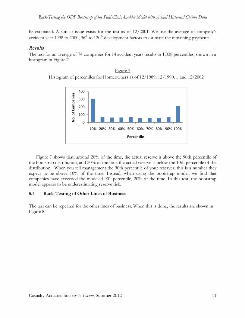
Back-Testing the ODP Bootstrap of the Paid Chain-Ladder Model with Actual Historical Claims Data
Casualty Actuarial Society E-Forum, Summer 2012 11
be estimated. A similar issue exists for the test as of 12/2001. We use the average of company’s accident year 1998 to 2000, 96th to 120th development factors to estimate the remaining payments.
Results The test for an average of 74 companies for 14 accident years results in 1,038 percentiles, shown in a histogram in Figure 7.
Figure 7 Histogram of percentiles for Homeowners as of 12/1989, 12/1990… and 12/2002
Figure 7 shows that, around 20% of the time, the actual reserve is above the 90th percentile of
the bootstrap distribution, and 30% of the time the actual reserve is below the 10th percentile of the distribution. When you tell management the 90th percentile of your reserves, this is a number they expect to be above 10% of the time. Instead, when using the bootstrap model, we find that companies have exceeded the modeled 90th percentile, 20% of the time. In this test, the bootstrap model appears to be underestimating reserve risk.
5.4 Back-Testing of Other Lines of Business
The test can be repeated for the other lines of business. When this is done, the results are shown in Figure 8.
0
100
200
300
400
10% 20% 30% 40% 50% 60% 70% 80% 90% 100%
No.
of C
ompa
nies
Percentile
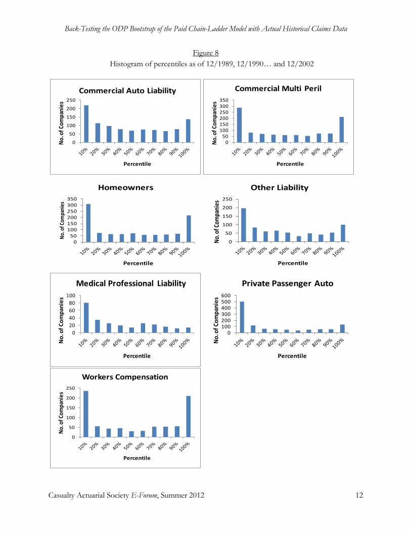
Back-Testing the ODP Bootstrap of the Paid Chain-Ladder Model with Actual Historical Claims Data
Casualty Actuarial Society E-Forum, Summer 2012 12
Figure 8 Histogram of percentiles as of 12/1989, 12/1990… and 12/2002
0
50
100
150
200
250
No. o
f Com
pani
es
Percentile
Commercial Auto Liability
050
100150200250300350
No. o
f Com
pani
es
Percentile
Commercial Multi Peril
0
50
100
150
200
250
No. o
f Com
pani
es
Percentile
Workers Compensation
0
50
100
150
200
250
No. o
f Com
pani
es
Percentile
Other Liability
050
100150200250300350
No. o
f Com
pani
es
Percentile
Homeowners
020406080
100
No.
of C
ompa
nies
Percentile
Medical Professional Liability
0100200300400500600
No. o
f Com
pani
es
Percentile
Private Passenger Auto

Back-Testing the ODP Bootstrap of the Paid Chain-Ladder Model with Actual Historical Claims Data
Casualty Actuarial Society E-Forum, Summer 2012 13
The histograms above do not follow a uniform distribution. In this test, for most of these lines of business, using the bootstrap model has produced distributions that underestimate reserve risk. However, for medical professional liability and private passenger auto in particular, it appears that the paid chain-ladder method is producing reserve estimates that are biased high.
6. ANALYSIS OF THE RESULTS A reserve distribution is a measure of how the actual unpaid loss may deviate from the best
estimate. By applying the ODP bootstrap to the paid chain-ladder method, we can get such a reserve distribution around a paid chain-ladder best estimate.
However, it is rare to rely solely on this method to determine an actuarial central reserve estimate. For better or worse, it is common practice for actuaries to estimate a distribution by using a similar ODP bootstrap of the chain-ladder method outlined here, and then “shift” this distribution by multiplication so that the mean is the same as an actuarial best estimate reserve or booked reserve.
We do not condone this practice, but it is so common that a natural question is whether the “shifting” of the distributions produced in our back-testing would result in a more uniform distribution. Booked reserve estimates use more sophisticated methods than the paid chain-ladder model, and therefore may be more accurate, so the width of the distributions being produced in this study may be perfectly suitable. If we used the booked reserve then we may not have seen the under- and over-reserving in the December 2000 and December 1996 results, respectively
In reality, the industry does under- and over-reserve, sometimes significantly. In comparison to the paid chain-ladder method, the industry is sometimes better or worse at estimating the true unpaid loss. In Figure 9, we show the booked ultimate loss at 12, 24, 36… and 120 months of evaluation, divided by the booked ultimate loss at the 12-month evaluation, for the U.S. industry, in aggregate for the seven lines of business tested in this paper.
The “PCL” line on this graph shows the cumulative paid loss and ALAE at 120 months of evaluation divided by the PCL estimate at 12 months of evaluation (using an all year weighted average on an industry 10 accident year triangle by line of business and excluding a tail factor).

Back-Testing the ODP Bootstrap of the Paid Chain-Ladder Model with Actual Historical Claims Data
Casualty Actuarial Society E-Forum, Summer 2012 14
Figure 9 Booked ultimate loss at t months of evaluation / Booked ultimate loss at 12 months of evaluation,
in aggregate for the industry for seven lines of business, net of reinsurance
For example, for accident year 2000, the booked ultimate loss estimate as of 12/2009 ended up 12% higher than the initial booked ultimate loss as of 12/2000. In contrast, the paid chain-ladder estimate of the ultimate loss as of 12/2009 was the same as the estimate as of 12/2000 – that is, the paid chain-ladder reserve estimate as of 12/2000 was more accurate than the booked reserve.7
Shifting a distribution around another mean is not a sound practice. Even ignoring this, we did not feel that shifting the mean to equal the booked reserve at the time would have materially changed the broad result of our back-testing.
6.1 Why are we seeing these results?
In an Institute of Actuaries of Australia report titled, “A Framework for Assessing Risk Margins,” 8
the sources of uncertainty in a reserve estimate are grouped into two parts: independent risk and systemic risk.
1. Independent risk = “risks arising due to the randomness inherent in the insurance process.” 2. Systemic risk = a risk that affects a whole system. “Risks that are potentially common across
valuation classes or claim groups.”8 Even if the model is accurately reflecting the claims process today, future trends in claims experience may move systematically away from what
7 Note that the comparison is not exact – the “PCL” line excludes all payments after 120 months whereas the booked reserves include those payments, which must add to the difficulty of estimation. Additionally, the booked reserve is estimated at a company level where as the “PCL” line was estimated using a whole industry loss triangle by line of business. 8 IAAust Risk Margins Task Force (2008).
0.70
0.75
0.80
0.85
0.90
0.95
1.00
1.05
1.10
1.15
1.20
1980
1982
1984
1986
1988
1990
1992
1994
1996
1998
2000
2002
2004
2006
2008
2010Book
ed U
ltim
ate
Loss
(t) /
Boo
ked
Ulti
mat
e Lo
ss (1
2)
Accident Year
'12/12 24/12 36/12 48/12 60/12 72/12
84/12 96/12 108/12 120/12 PCL

Back-Testing the ODP Bootstrap of the Paid Chain-Ladder Model with Actual Historical Claims Data
Casualty Actuarial Society E-Forum, Summer 2012 15
was experienced in the past. For example, unexpected changes in inflation, unexpected tort reform or unexpected changes in legislation.
They state that the traditional quantitative techniques, such as bootstrapping, are better at
analyzing independent risk but aren’t able to adequately capture systemic risk. This is because, even if there are past systemic episodes in the data, “a good stochastic model will fit the past data well and, in doing so, fit away most past systemic episodes of risk…leaving behind largely random sources of uncertainty.” 8
The distributions produced in this paper using the bootstrap model may be underestimating reserve risk because they only capture independent risk, not systemic risk.
7. POSSIBLE ADJUSTMENTS TO THE METHOD If the ODP bootstrap of the paid chain-ladder method is producing distributions that
underestimate the true reserve risk, then what adjustments can be made so that it more accurately captures the risk?
7.1 Commonly used possible adjustments
Bootstrapping the incurred chain-ladder method
Using the method outlined in this paper on incurred loss and ALAE data instead of paid loss and ALAE data produces reserve distributions with a smaller variance. This is understandable if you assume that the case reserves provide additional information about the true cost of future payments. We back-tested the incurred bootstrap model for the Workers Compensation line of business. The process was the same as for the paid bootstrap model, but incurred loss and ALAE was substituted for the paid loss and ALAE data, resulting in distributions of IBNR. The resulting percentiles are in Figure 10.

Back-Testing the ODP Bootstrap of the Paid Chain-Ladder Model with Actual Historical Claims Data
Casualty Actuarial Society E-Forum, Summer 2012 16
Figure 10 Histogram of percentiles for Workers Compensation as of 12/1989, 12/1990….. 12/2002 based on
incurred loss & ALAE
From Figure 10, it appears that the incurred bootstrap model is also underestimating the risk of falling in these extreme percentiles.
Using more historical years of paid loss and ALAE data
Our back-testing used paid loss and ALAE triangles with 10 historical accident and development years. A loss triangle with more historical accident years may result in a wider distribution.
We applied the bootstrap model on 20 accident year x 10 development year homeowners paid loss and ALAE triangles, but this resulted in distributions that sometimes had more and sometimes had less variability than the original distributions from the 10 x 10-year datasets.
Making Other Adjustments
There are other additions to the bootstrap model that we have not considered here, and can be areas of further study:
• Parametric bootstrapping. It is possible to simulate the accident year and development year parameters from a multivariate normal distribution using a generalized linear model, which closely follows the structure of the ODP bootstrap of the paid chain-ladder model. This is commonly called parametric bootstrapping. Re-sampling the residuals, as outlined in section 3, may be limiting, and simulating from a normal distribution may result in wider reserve distributions.
• Hat matrix. The hat matrix can be applied to standardize the Pearson residuals and make them identically distributed, as per Pinheiro, Andrade e Silva, and Centeno (2003).
• Multiple scale parameters to account for heteroskedasticity in residuals.
None of these commonly used adjustments are specifically designed to account for systemic risk. Also, the method we are testing significantly underestimates the true risk and so requires an
0
50
100
150
200
No.
of C
ompa
nies
Percentile

Back-Testing the ODP Bootstrap of the Paid Chain-Ladder Model with Actual Historical Claims Data
Casualty Actuarial Society E-Forum, Summer 2012 17
adjustment that significantly widens the distribution. Therefore, we outline below two methods that can be applied to the bootstrap model that account for systemic risk.
7.2 Two methods to account for systemic risk
We have derived two methods to adjust the ODP bootstrap of the paid chain-ladder model so that the resulting distributions of unpaid loss and ALAE describe the true reserve risk – that is, it passes our back-testing, so that, for example, 10% of the time the actual reserve falls above the 90th percentile of our estimated distribution. These two methods are explicitly attempting to model systemic risk – the risk that the future claims environment is different from the past.
The two methods are: 1. The systemic risk distribution method 2. Wang transform adjustment
The two methods are based on two different assumptions. The systemic risk distribution
method does not adjust the actuary’s central estimate over the reserving cycle. The Wang transform adjustment does not assume that the central estimate reserve is unbiased and tries to estimate the systemic bias of the chain-ladder method over the course of reserving cycle.
Both methods are applied and the resulting distribution is back-tested again.
Systemic Risk Distribution Method As outlined in section 6.1, reserve risk can be broken down into two parts: (1) independent
risk and (2) systemic risk. We believe that the bootstrap model only measures independent risk, not systemic risk. Systemic risk affects a whole system, like the market of insurers. It includes risks such as unexpected changes in inflation and unexpected changes in tort reform – in short, the risk that the future claims environment could be different from the past.
In this method, we estimate a benchmark systemic risk distribution by line of business, and combine this with the independent risk distribution (from the bootstrap model) to obtain the total reserve risk distribution. To combine the distributions we assume that they are independent from each other, and take one simulation from the systemic risk distribution and multiply this by one simulation from the independent risk distribution, and repeat for all 10,000 (or more) iterations.

Back-Testing the ODP Bootstrap of the Paid Chain-Ladder Model with Actual Historical Claims Data
Casualty Actuarial Society E-Forum, Summer 2012 18
Figure 11 Example of one iteration of the systemic risk distribution adjustment
Each of the outcomes from the systemic risk distribution, such as the 1.13 in Figure 11, can
be thought of as a systemic risk factor. We can calculate historical systemic risk factors for each year and for each company by the following procedure:
1. Take the mean of the bootstrap model’s reserve distribution for each company, as of 12/1989 for accident year 1989.
2. Calculate what the reserve should have been for accident year 1989, back in 12/1989 (= the ultimate loss and ALAE as of 12/2008 less the paid as of 12/1989).
3. The systemic risk factor = (2)/(1). 4. Repeat 1 to 3 as of 12/1990, 12/1991, ….to 12/2002.
The systemic risk benchmark distribution is estimated by fitting a distribution to the
historical systemic risk factors. Through a curve-fitting exercise, we found that a Gamma distribution was the best candidate to model systemic risk, with differing parameters by line of business. This results in uniform distributions of percentiles when the method outlined above is back-tested, as shown in Figure 12.
Admittedly, the fitted systemic risk distribution may differ depending on the back-testing period. However, we took care to span a time period that incorporated one upwards and one downwards period of the reserve cycle, in an attempt to not bias the results.

Back-Testing the ODP Bootstrap of the Paid Chain-Ladder Model with Actual Historical Claims Data
Casualty Actuarial Society E-Forum, Summer 2012 19
Figure 12 Histogram of Percentiles as of 12/1989, 12/1990… to 12/2002
0
50
100
150
No.
of C
ompa
nies
Percentile
Commercial Auto Liability
020406080
100120140
No.
of C
ompa
nies
Percentile
Commercial Multi Peril
020406080
100
No. o
f Com
pani
es
Percentile
Other Liability
020406080
100120140
No. o
f Com
pani
es
Percentile
Homeowners
0
10
20
30
40
No. o
f Com
pani
es
Percentile
Medical Professional Liability
0
50
100
150
No. o
f Com
pani
es
Percentile
Private Passenger Auto
0
20
40
60
80
100
120
No. o
f Com
panie
s
Percentile
Workers Compensation

Back-Testing the ODP Bootstrap of the Paid Chain-Ladder Model with Actual Historical Claims Data
Casualty Actuarial Society E-Forum, Summer 2012 20
As an example, for Homeowners, the systemic risk distribution is a gamma distribution with a mean of 0.98 and a standard deviation of 19%. Note that this is intended to adjust the distribution of the reserve for a single accident year at 12 months of evaluation.
Systemic risk has its roots in the reserving cycle and underwriting cycle. Indeed, there are documented evidences of the linkage between reserving cycle and underwriting cycle. Archer-Lock et al. (2003) discussed reserving cycle in the U.K. The authors conclude that the mechanical application of traditional actuarial reserving methods may be one of the causes for reserve cycle. In particular, the underwriting cycle may distort claims development patterns and that premium rates indices may understate the magnitude of the cycle. The Wang transform adjustment is an alternative systemic risk adjustment that explicitly accounts for the reserve cycle.
Wang-Transform Adjustment
The Wang transform adjustment method does not assume that the unpaid loss and ALAE estimate is unbiased and tries to estimate the systemic bias over the course of reserving cycle. The reserving cycle shown in Figure 13 is an interesting phenomenon that indicates that reserve risk is cyclical, and the Wang transform adjustment method tries to capture this “systemic” bias.
We use the workers compensation line of business for illustration. The data used in back-testing is the workers compensation aggregated industry data net incurred loss and ALAE. A series of back-tests (these back-tests are different from the test in section 4) are done using the chain-ladder method for industry loss reserve development. For accident years after 2001, we use the latest reported losses instead of the projected ultimate losses, since reported losses for those accident years are not yet fully developed.
In the following figures, which represent the entire non-life industry workers compensation line of business, Ultimate Losses (UL) stand for the 120-month incurred loss and ALAE for each accident year (AY) from the latest report year (RY), not including IBNR. Initial Losses (IL) represent the projected 120-month net incurred loss and ALAE for each AY from first report year, using the chain-ladder reserving method. Ultimate Loss Ratio (ULR) represents the ultimate reported incurred loss and ALAE ratio for each AY and Initial Loss Ratio (ILR) represents the initial reported incurred loss ratio for each AY. A more detailed explanation of the back-testing method is given in Appendix B.

Back-Testing the ODP Bootstrap of the Paid Chain-Ladder Model with Actual Historical Claims Data
Casualty Actuarial Society E-Forum, Summer 2012 21
Figure 13 Chain-Ladder Method Back-Testing Error versus (ULR-ILR) for Workers Compensation
For the workers compensation line of business, the chain-ladder reserving method has systematic errors that are highly correlated with the reserving cycle. The contemporary correlation between the estimation error and the reserve development (ULR-ILR) is 0.64 for the chain-ladder method. More noticeably, the one-year lag correlation is 0.91. The estimation error leads the loss reserve development by one-year.
In this study, we apply the Wang transform to enhance the loss reserve distribution created using the bootstrap of the chain-ladder method. Different from the systemic risk distribution method, the Wang transform adjustment method will first adjust the variability of the loss reserve then give each company group’s loss reserve distribution a shift, respectively.
The procedures below describe how to apply the Wang-Transform adjustment:
1. After bootstrapping each paid loss triangle with 10,000 iterations, we apply the ratio of double exponential over normal to adjust the chain-ladder reserve distribution to be wider than the original distribution. The formula is shown below:
𝑥𝑥∗ = (𝑥𝑥 − 𝑢𝑢) ∗ ratio + 𝑢𝑢
ratio(𝑞𝑞) = exponential−1(𝑞𝑞)/ϕ−1(𝑞𝑞)
Where:
1) ϕ is a normal distribution with mean 0 and standard deviation 1. 2) Exponential stands for a double exponential distribution with density function
𝑓𝑓(𝑥𝑥) = 0.5 ∗ λ ∗ e−λ∗|𝑥𝑥|,−∞ < 𝑥𝑥 < ∞. 3) q is the quantile of each simulated reserve. 4) u is the median of 10,000 simulated reserves.
-20%-15%-10%-5%0%5%10%15%20%25%
(4,000,000)(3,000,000)(2,000,000)(1,000,000)
-1,000,000 2,000,000 3,000,000 4,000,000
1990
1991
1992
1993
1994
1995
1996
1997
1998
1999
2000
2001
2002
2003
2004
ULR
-ILR
$(00
0) U
L-IL
Accident Year
UL-IL(Estimation Error) ULR-ILR

Back-Testing the ODP Bootstrap of the Paid Chain-Ladder Model with Actual Historical Claims Data
Casualty Actuarial Society E-Forum, Summer 2012 22
5) x is the simulated reserve. 6) x* is the reserve after adjustment.
2. β is calculated for each company to measure the correlation between the company and industry.
The method to calculate the β is described below: For each AY, if the industry systemic risk factor is significantly different from one (greater than 1.01 or less than 0.99), we use an indicator of +1 if a company’s corresponding AY systemic risk ratio is in the same direction as the industry systemic risk factor, otherwise we use an indicator of -1. For example, say the industry systemic risk factor for AY 2000 is 1.122, which is greater than 1. If company A’s AY 2000 systemic risk factor is greater than 1, we assign an indicator of +1 to company A AY 2000. If company B’s AY 2000 systemic risk factor is less than 1, we assign an indicator of -1 to company B AY 2000. At last, for a company, β = (sum of indicators of all AYs) / (count of indicators of all AYs). If β is less than zero, we force it to zero.
3. The Wang transform is finally applied to adjust the mean of the reserve distribution. The formula is shown below:
F2(x) = ϕ�ϕ−1�F1(x)� + β ∗ λ�. Where: 1) F1(x) is reported reserve’s percentile in the reserve distribution after step 1
adjustment. 2) Each company has its own β value. 3) ϕ is a normal distribution with mean 0 and standard deviation 1.
We change λ to result in the most uniformly distributed percentiles as measured by a chi-square test, when the adjusted reserve is back-tested. λ here is the fitted shift value of loss reserve distribution for each accident year.
The final λs are shown in the following figures.
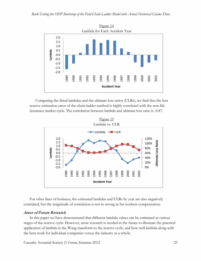
Back-Testing the ODP Bootstrap of the Paid Chain-Ladder Model with Actual Historical Claims Data
Casualty Actuarial Society E-Forum, Summer 2012 23
Figure 14 Lambda for Each Accident Year
Comparing the fitted lambdas and the ultimate loss ratios (ULRs), we find that the loss reserve estimation error of the chain-ladder method is highly correlated with the non-life insurance market cycle. The correlation between lambda and ultimate loss ratio is -0.87.
Figure 15 Lambda vs. ULR
For other lines of business, the estimated lambdas and ULRs by year are also negatively correlated, but the magnitude of correlation is not as strong as for workers compensation.
Areas of Future Research In this paper we have demonstrated that different lambda values can be estimated at various
stages of the reserve cycle. However, more research is needed in the future to illustrate the practical application of lambda in the Wang transform to the reserve cycle, and how well lambda along with the beta work for individual companies versus the industry as a whole.
-2.0-1.5-1.0-0.50.00.51.01.52.0
1989
1990
1991
1992
1993
1994
1995
1996
1997
1998
1999
2000
2001
2002
Lam
bda
Accident Year
0%20%40%60%80%100%120%
-2.0-1.5-1.0-0.50.00.51.01.52.0
1989
1990
1991
1992
1993
1994
1995
1996
1997
1998
1999
2000
2001
2002
Ulti
mat
e Lo
ss R
atio
Lam
bda
Accident Year
Lambda ULR

Back-Testing the ODP Bootstrap of the Paid Chain-Ladder Model with Actual Historical Claims Data
Casualty Actuarial Society E-Forum, Summer 2012 24
In this paper, we have focused mostly on the paid loss development method. Another area of future research is to investigate the difference between using paid methods in isolation versus paid loss development methods in conjunction with case incurred loss development methods, exposure-based methods, and judgment.
Yet another area of future research is to investigate the reserve cycle illustrated in Figure 9.
8. SUMMARY The genesis and popularity of a reserve risk method lies in its theoretical beauty. However, as
more insurers rely on actuarial estimates of reserve risk to manage capital, estimating a reserve distribution is no longer a purely theoretical exercise. Methods should be tested against real data9
In this back-test, we see that the popular ODP bootstrap of the paid chain-ladder method is underestimating reserve risk. We believe that it is because the bootstrap model does not consider systemic risk, or, to put it another way, the risk that future trends in the claims environment — such as inflation, trends in tort reform, legislative changes, etc. — may deviate from what we saw in the past. We suggest two simple solutions to incorporate systemic risk into the reserve distribution so that the adjusted reserve distribution passes the back-test.
before they can be relied upon to support the insurance industry’s solvency.
We hope to encourage more testing of models so that the profession has a more defensible framework for measuring risks for solvency and profitability.
9 We advocate the use of real versus simulated data. In this paper, we have found that the bootstrap model, for most lines, materially underestimates the probability of falling above the 90th percentile. In contrast, the same model when tested against simulated data in GIRO, found that the same bootstrap model identified a 99th percentile that was exceeded only 1% to 4% of the time by the simulated data.

Back-Testing the ODP Bootstrap of the Paid Chain-Ladder Model with Actual Historical Claims Data
Casualty Actuarial Society E-Forum, Summer 2012 25
Appendix A: The ODP bootstrap of the paid chain-ladder method that was tested
We are testing the reserve distribution created using the bootstrap of the paid chain-ladder method. The model we are using is described in Appendix 3 of England and Verrall (2002). We detail this, with a numerical example, below:
1. Take a paid loss and ALAE, 10 accident year by 10 development year triangle
Figure A1 Company A, paid Loss & ALAE, net of reinsurance as of 12/2000
Data in $ millions
AY 1 2 3 4 5 6 7 8 9 10 1991 94 119 124 128 130 132 133 133 133 134 1992 101 131 135 139 141 143 143 144 145 1993 82 107 112 116 119 119 120 121 1994 110 139 146 152 154 155 156 1995 68 99 105 108 111 114 1996 119 151 157 158 162 1997 72 99 99 99 1998 71 101 106 1999 71 96 2000 62
2. Calculate the all-year, volume-weighted age-to-age factors.
Figure A2
1 - 2 2 - 3 3 - 4 4 - 5 5 - 6 6 - 7 7 - 8 8 - 9 9 - 10 1.32 1.04 1.02 1.02 1.01 1.00 1.00 1.00 1.00

Back-Testing the ODP Bootstrap of the Paid Chain-Ladder Model with Actual Historical Claims Data
Casualty Actuarial Society E-Forum, Summer 2012 26
3. Estimate a fitted triangle by taking the cumulative paid loss and ALAE to date from (1).
Figure A3 Company A, paid Loss & ALAE to date, net of reinsurance as of 12/2000
Data in $ millions
AY 1 2 3 4 5 6 7 8 9 10 1991 134 1992 144 1993 121 1994 156 1995 114 1996 162 1997 99 1998 106 1999 96 2000 62
4. Estimate the fitted historical cumulative paid loss and ALAE by using (2) to un-develop (3).
Figure A4
Company A, paid Loss & ALAE, net of reinsurance as of 12/2000 Data in $ millions
AY 1 2 3 4 5 6 7 8 9 10 1991 90 120 125 128 130 132 132 133 133 134 1992 98 129 135 138 141 143 143 144 144 1993 82 108 113 116 118 120 120 121 1994 107 141 147 150 153 155 156 1995 78 103 108 110 112 114 1996 112 149 155 159 162 1997 70 93 97 99 1998 77 102 106 1999 72 96 2000 62
5. Calculate the unscaled Pearson residuals, 𝑟𝑟𝑝𝑝 (from England and Verrall 1999).
𝑟𝑟𝑝𝑝 = 𝐶𝐶−𝑚𝑚√𝑚𝑚
,
= 96 / 1.32

Back-Testing the ODP Bootstrap of the Paid Chain-Ladder Model with Actual Historical Claims Data
Casualty Actuarial Society E-Forum, Summer 2012 27
where 𝐶𝐶 = incremental actual loss from step (1) and 𝑚𝑚 = incremental fitted loss from step (4).
Figure A5
Company A, unscaled residuals, net of reinsurance as of 12/2000
AY 1 2 3 4 5 6 7 8 9 10 1991 0.35 (0.76) 0.13 0.55 (0.38) 0.14 0.44 (0.37) (0.06) 1992 0.35 (0.39) (0.39) 0.12 (0.42) 0.32 (0.61) 0.05 0.05 1993 (0.03) (0.18) 0.07 0.55 0.73 (0.92) 0.07 0.33 1994 0.32 (0.89) 0.52 1.21 (0.64) (0.43) 0.12 1995 (1.14) 1.12 1.03 0.24 0.51 0.94 1996 0.65 (0.79) (0.08) (1.27) 0.31 1997 0.16 1.00 (1.92) (1.49) 1998 (0.67) 0.97 0.51 1999 (0.23) 0.40 2000
6. Calculate the degrees of freedom and the scale parameter:
𝐷𝐷𝐷𝐷𝐷𝐷 = 𝑛𝑛 − 𝑝𝑝 = 55 − 19
= 36
where 𝐷𝐷𝐷𝐷𝐷𝐷 = degrees of freedom, 𝑛𝑛 = number of incremental loss and ALAE data points in the triangle in step 1, and 𝑝𝑝 = number of parameters in the paid chain-ladder model (in this case, 10 accident year parameters and 9 development year parameters).
𝑆𝑆𝑆𝑆𝑆𝑆𝑆𝑆𝑆𝑆 𝑃𝑃𝑆𝑆𝑟𝑟𝑆𝑆𝑚𝑚𝑆𝑆𝑃𝑃𝑆𝑆𝑟𝑟 =∑𝑟𝑟𝑝𝑝2
𝐷𝐷𝐷𝐷𝐷𝐷
=24.136
= 0.669.
7. Adjust the unscaled Pearson residuals (𝑟𝑟𝑝𝑝) calculated in step 5:
=(71 − 72)√72

Back-Testing the ODP Bootstrap of the Paid Chain-Ladder Model with Actual Historical Claims Data
Casualty Actuarial Society E-Forum, Summer 2012 28
𝑟𝑟𝑝𝑝𝑆𝑆𝑎𝑎𝑎𝑎 = �
𝑛𝑛𝐷𝐷𝐷𝐷𝐷𝐷
× 𝑟𝑟𝑝𝑝
= �5536
× 𝑟𝑟𝑝𝑝
= 1.24 × 𝑟𝑟𝑝𝑝 .
Figure A6
𝑟𝑟𝑝𝑝𝑆𝑆𝑎𝑎𝑎𝑎 : Company A, unscaled residuals, net of reinsurance as of 12/2000
AY 1 2 3 4 5 6 7 8 9 10 1991 0.43 (0.94) 0.17 0.68 (0.47) 0.17 0.55 (0.45) (0.07) 1992 0.43 (0.48) (0.48) 0.15 (0.52) 0.39 (0.76) 0.07 0.07 1993 (0.04) (0.22) 0.09 0.68 0.90 (1.14) 0.09 0.40 1994 0.40 (1.09) 0.64 1.49 (0.79) (0.53) 0.15 1995 (1.41) 1.38 1.27 0.30 0.63 1.17 1996 0.80 (0.98) (0.10) (1.58) 0.39 1997 0.19 1.23 (2.38) (1.85) 1998 (0.83) 1.20 0.63 1999 (0.28) 0.50 2000
8. Sample from the adjusted Pearson residuals 𝑟𝑟𝑝𝑝𝑆𝑆𝑎𝑎𝑎𝑎 in step 7, with replacement.
Figure A7
Company A, Sampled adjusted residuals, net of reinsurance as of 12/2000
AY 1 2 3 4 5 6 7 8 9 10 1991 (1.09) (0.28) (0.04) 0.07 0.17 (0.07) 1.20 0.63 1.27 (0.28) 1992 (0.28) 0.43 0.39 0.80 (0.53) 1.17 0.19 (0.98) (0.48) 1993 0.09 0.39 (0.94) 1.20 (0.83) (0.53) 0.63 (0.76) 1994 0.68 (2.38) 1.23 (0.98) 0.30 0.43 (1.14) 1995 (0.47) (0.94) 0.50 (0.48) 0.15 (0.94) 1996 0.63 0.15 (1.14) 1.49 1.49 1997 0.07 0.07 0.17 (2.38) 1998 0.15 0.63 0.39 1999 1.20 0.50 2000 0.50
9. Calculate the triangle of sampled incremental loss, 𝐶𝐶.
= (0.23)

Back-Testing the ODP Bootstrap of the Paid Chain-Ladder Model with Actual Historical Claims Data
Casualty Actuarial Society E-Forum, Summer 2012 29
𝐶𝐶 = 𝑚𝑚 + 𝑟𝑟𝑝𝑝𝑆𝑆𝑎𝑎𝑎𝑎 √𝑚𝑚.
Figure A8
Company A, sampled incremental paid Loss & ALAE, net of reinsurance as of 12/2000 Data in $ millions
AY 1 2 3 4 5 6 7 8 9 10 1991 80 28 5 3 3 2 1 1 1 0 1992 95 34 6 5 2 4 1 (0) 0 1993 83 28 3 5 1 1 1 (0) 1994 114 20 9 2 3 3 (0) 1995 74 20 5 2 2 0 1996 119 37 3 6 6 1997 71 23 4 (1) 1998 78 28 5 1999 83 26 2000 65
10. Project the future paid loss and ALAE, using the paid chain-ladder method.
Figure A9
Company A, cumulative paid Loss & ALAE, net of reinsurance as of 12/2000 Data in $ millions
AY 1 2 3 4 5 6 7 8 9 10 1991 80 108 113 116 118 120 121 122 124 124 1992 95 129 136 140 142 146 146 146 146 147 1993 83 111 114 118 119 120 121 121 122 122 1994 114 134 143 145 148 151 151 151 152 152 1995 74 94 100 102 104 104 105 105 106 106 1996 119 156 160 166 172 175 175 176 177 177 1997 71 94 98 97 99 101 101 101 102 102 1998 78 106 112 114 117 118 119 119 120 120 1999 83 108 113 116 118 120 121 121 122 122 2000 65 86 89 92 93 95 95 96 96 96
Weighted average age-to-age factors
1 - 2 2 - 3 3 - 4 4 – 5 5 - 6 6 - 7 7 - 8 8 - 9 9 - 10 1.31 1.04 1.02 1.02 1.02 1.00 1.00 1.01 1.00
11. Include process variance by simulating each incremental future loss and ALAE from a Gamma
distribution with:
= 72 + 1.20 ∗ √72
= 65 × 1.31

Back-Testing the ODP Bootstrap of the Paid Chain-Ladder Model with Actual Historical Claims Data
Casualty Actuarial Society E-Forum, Summer 2012 30
mean = projected incremental losses in step 10, variance = mean x scale parameter from step 6.
We assume that each future incremental loss is independent from each other. Note that theoretically we assume an over-dispersed Poisson distribution, however, we are using the Gamma distribution as a close approximation.
Figure A10 Company A, incremental paid Loss & ALAE, with process variance, net of reinsurance as of
12/2000 Data in $ millions
AY 1 2 3 4 5 6 7 8 9 10 1991 82 28 5 3 3 2 1 1 1 0 1992 96 34 6 4 2 3 1 0 0 0 1993 83 28 3 4 1 1 1 0 1 0 1994 112 23 8 2 3 3 (0) 0 2 1 1995 75 21 5 2 2 1 0 1 1 0 1996 118 37 4 6 5 4 2 0 0 0 1997 71 23 4 (1) 2 4 0 1 1 1 1998 78 27 5 4 2 0 1 0 0 0 1999 81 25 3 2 1 1 0 0 0 1 2000 65 18 5 2 1 1 1 0 0 0
= 𝐺𝐺𝑆𝑆𝑚𝑚𝑚𝑚𝑆𝑆(𝑚𝑚𝑆𝑆𝑆𝑆𝑛𝑛 = 21,𝑣𝑣𝑆𝑆𝑟𝑟𝑣𝑣𝑆𝑆𝑛𝑛𝑆𝑆𝑆𝑆 = 0.669 ∗ 21)

Back-Testing the ODP Bootstrap of the Paid Chain-Ladder Model with Actual Historical Claims Data
Casualty Actuarial Society E-Forum, Summer 2012 31
12. Estimate the unpaid loss and ALAE by taking a sum of the future incremental losses from step 11.
Figure 11 Unpaid Accident Loss
year and ALAE 1991 0 1992 0 1993 1 1994 3 1995 2 1996 6 1997 9 1998 7 1999 8 2000 28
Total 64
13. Repeat steps 8 to 12. In our case, 10,000 times to produce 10,000 unpaid loss and ALAE
estimates resulting in an unpaid loss and ALAE distribution when plotted in a histogram.

Back-Testing the ODP Bootstrap of the Paid Chain-Ladder Model with Actual Historical Claims Data
Casualty Actuarial Society E-Forum, Summer 2012 32
Appendix B Methodology for Reserving Back-Testing The method used in back-testing in the Wang transform adjustment uses 10 accident year by 10 development year incurred loss and ALAE triangles, net of reinsurance.
The UL is the 120-month, case-incurred loss for each AY. For example, for AY 2001, the UL is yellow highlighted cell below.
IL stands for the projected 120-month, case-incurred loss for each AY from first RY. For example, for AY 2001, the IL is projected from the triangle below.
AY NetCaseIncurred2001 10,597,343 15,121,875 17,148,317 18,030,720 18,315,025 18,663,494 18,963,470 19,274,423 19,492,073 19,691,532 2002 9,880,312 14,375,596 16,125,066 16,778,143 17,329,085 17,651,826 17,996,103 18,251,653 18,518,021 2003 10,369,458 14,334,644 15,837,509 16,594,323 17,191,600 17,714,263 17,992,600 18,339,834 2004 10,616,734 14,461,802 15,894,418 16,644,316 17,253,999 17,678,604 18,059,807 2005 11,234,028 14,723,765 16,219,677 17,166,414 17,739,780 18,273,742 2006 11,762,138 15,866,737 17,804,050 18,942,686 19,777,903 2007 12,189,806 16,932,637 19,062,769 20,387,578 2008 12,394,686 17,351,056 19,656,367 2009 11,230,304 15,726,363 2010 11,564,142 2000 10,300,006 15,323,250 17,359,275 18,504,064 19,310,172 19,727,612 20,024,743 20,349,723 20,416,586 20,626,383 2001 10,597,343 15,121,875 17,148,317 18,030,720 18,315,025 18,663,494 18,963,470 19,274,423 19,492,073 2002 9,880,312 14,375,596 16,125,066 16,778,143 17,329,085 17,651,826 17,996,103 18,251,653 2003 10,369,458 14,334,644 15,837,509 16,594,323 17,191,600 17,714,263 17,992,600 2004 10,616,734 14,461,802 15,894,418 16,644,316 17,253,999 17,678,604 2005 11,234,028 14,723,765 16,219,677 17,166,414 17,739,780 2006 11,762,138 15,866,737 17,804,050 18,942,686 2007 12,189,806 16,932,637 19,062,769 2008 12,394,686 17,351,056 2009 11,230,304
2001 10,597,343 15,121,875 17,148,317 18,030,720 18,315,025 18,663,494 18,963,470 19,274,423 19,492,073 19,691,532 2002 9,880,312 14,375,596 16,125,066 16,778,143 17,329,085 17,651,826 17,996,103 18,251,653 18,518,021 2003 10,369,458 14,334,644 15,837,509 16,594,323 17,191,600 17,714,263 17,992,600 18,339,834 2004 10,616,734 14,461,802 15,894,418 16,644,316 17,253,999 17,678,604 18,059,807 2005 11,234,028 14,723,765 16,219,677 17,166,414 17,739,780 18,273,742 2006 11,762,138 15,866,737 17,804,050 18,942,686 19,777,903 2007 12,189,806 16,932,637 19,062,769 20,387,578 2008 12,394,686 17,351,056 19,656,367 2009 11,230,304 15,726,363 2010 11,564,142
1992 13,577,454 18,324,228 19,318,317 19,887,417 20,329,004 20,578,733 20,829,649 21,093,165 21,251,010 21,445,507 1993 11,629,774 15,072,352 16,240,909 17,019,006 17,377,062 17,817,291 17,991,759 18,151,739 18,369,115 1994 10,064,429 13,048,331 14,255,204 14,761,320 15,191,420 15,488,568 15,640,632 15,907,265 1995 9,091,097 12,075,438 13,156,052 13,952,635 14,395,087 14,703,283 14,936,659 1996 9,272,956 12,274,028 13,702,650 14,407,800 14,920,371 15,315,039 1997 9,322,137 13,169,560 14,673,981 15,446,460 16,059,155 1998 10,192,450 14,078,543 15,775,394 16,820,701 1999 9,840,268 13,948,976 15,911,651 2000 10,300,006 15,323,250 2001 10,597,343

Back-Testing the ODP Bootstrap of the Paid Chain-Ladder Model with Actual Historical Claims Data
Casualty Actuarial Society E-Forum, Summer 2012 33
The red bold cells below are projected by chain-ladder method and the yellow highlighted cell is the IL.
1992 13,577,454 18,324,228 19,318,317 19,887,417 20,329,004 20,578,733 20,829,649 21,093,165 21,251,010 21,445,507 1993 11,629,774 15,072,352 16,240,909 17,019,006 17,377,062 17,817,291 17,991,759 18,151,739 18,369,115 18,537,236 1994 10,064,429 13,048,331 14,255,204 14,761,320 15,191,420 15,488,568 15,640,632 15,907,265 16,059,355 16,206,336 1995 9,091,097 12,075,438 13,156,052 13,952,635 14,395,087 14,703,283 14,936,659 15,125,933 15,270,552 15,410,313 1996 9,272,956 12,274,028 13,702,650 14,407,800 14,920,371 15,315,039 15,493,651 15,689,983 15,839,995 15,984,968 1997 9,322,137 13,169,560 14,673,981 15,446,460 16,059,155 16,419,983 16,611,482 16,821,978 16,982,814 17,138,246 1998 10,192,450 14,078,543 15,775,394 16,820,701 17,422,664 17,814,128 18,021,886 18,250,255 18,424,746 18,593,376 1999 9,840,268 13,948,976 15,911,651 16,820,875 17,422,844 17,814,313 18,022,073 18,250,444 18,424,936 18,593,568 2000 10,300,006 15,323,250 17,243,980 18,229,336 18,881,709 19,305,957 19,531,113 19,778,606 19,967,710 20,150,461 2001 10,597,343 15,145,457 17,043,901 18,017,824 18,662,628 19,081,953 19,304,497 19,549,118 19,736,028 19,916,659

Back-Testing the ODP Bootstrap of the Paid Chain-Ladder Model with Actual Historical Claims Data
Casualty Actuarial Society E-Forum, Summer 2012 34
References [1.] A.M. Best, “1969-2009 Impairment Review,” Best’s Special Report, June 21, 2010. [2.] Archer-Lock, P., et al., “The Cycle Survival Kit—An Investigation into the Reserving Cycle and Other Issues,”
paper presented at the 2003 General Insurance Convention. [3.] England, P., and R. Verrall, “Analytic and Bootstrap Estimates of Prediction Errors in Claims Reserving,”
Insurance: Mathematics and Economics 25 (1999):281–293. [4.] England, P., and R. Verrall, “Stochastic Claims Reserving in General Insurance,” British Actuarial Journal 8(3),
2002: 443-518. [5.] General Insurance Reserving Oversight (GIRO) Committee, Institute of Actuaries (U.K.), “Best Estimates and
Reserving Uncertainty,” paper presented at the 2007 GIRO conference. [6.] Meyers, G., and P. Shi, “The Retrospective Testing of Stochastic Loss Reserve Methods,” 2011 Summer CAS E-
Forum. [7.] Meyers, Glenn G., “Estimating Predictive Distributions for Loss Reserve Models,” Variance 1:2, 2007: 248-272. [8.] Pinheiro, P.J.R., J.M. Andrade e Silva, and M. De Lourdes Centeno, (2003), Bootstrap Methodology in Claim
Reserving. Journal of Risk and Insurance 70:701–714. [9.] Risk Margins Task Force, Institute of Actuaries of Australia, “A Framework for Assessing Risk Margins,” 2008,
paper presented at Institute of Actuaries of Australia 16th General Insurance Seminar, 9-12 November 2008.

Casualty Actuarial Society E-Forum, Summer 2012 1
The Leveled Chain Ladder Model for Stochastic Loss Reserving
Glenn Meyers, FCAS, MAAA, CERA, Ph.D.
_____________________________________________________________________________________________
Abstract: The popular chain ladder model forms its estimate by applying age-to-age factors to the latest reported cumulative claims amount – fixed numbers. This paper proposes two models that replace these fixed claim amounts with estimated parameters, which are subject to parameter estimation error. This paper uses a Bayesian Markov-Chain Monte Carlo (MCMC) method to estimate the predictive distribution of the total reported claims amountsfor these models. Using the CAS Loss Reserve Database, it tests its performance in predicting the distribution of outcomes on holdout data, from several insurers, for both paid and incurred triangles on four different lines of insurance. Their performance is compared with the performance of the Mack model on these data.
Key Words – Chain Ladder Model, Bayesian MCMC estimation, JAGS, Mack Model, Retrospective Testing of Loss Reserve Estimates, The R ChainLadder Package
_____________________________________________________________________________________________
1. INTRODUCTION
This paper presents two more stochastic loss reserving models. Probably the most generally accepted stochastic models, as evidenced by their inclusion in the CAS Syllabus of Examinations, are those of Mack [3] and England and Verrall [1]. The former paper estimates the moments of the predictive distribution of ultimate claims based on cumulative triangles of claims data. While providing a nice overview of the research to date, the latter paper focuses on estimating the predictive distribution of ultimate claims based on incremental triangles using a Generalized Linear Model (GLM).
While each of the models has a reasonable rationale and when implemented produce a predictive distribution of outcomes, large scale testing of the predictive distributions on actual outcomes was almost nonexistent until recently. One of the first to address the problem was Jessica Leong in her 2010 CLRS presentation1 where she concluded that the predictive distribution was too narrow for the homeowners’ data she analyzed. Last year, Meyers and Shi [6] created the CAS Loss Reserve Database.2
1Ms. Leong’s presentation can be downloaded from the CAS website at
This database was constructed by linking Schedule P reported losses over a period of ten years to outcomes of predictions made based on data reported in the first year. Meyers and Shi then tested two different models based on paid incremental losses and found that the performance of
http://www.casact.org/education/clrs/2010/handouts/VR6-Leong.pdf.
2The data and a complete description of its preparation can be found on the CAS Web site athttp://www.casact.org/research/index.cfm?fa=loss_reserves_data

The Leveled Chain Ladder Model for Stochastic Loss Reserving
Casualty Actuarial Society E-Forum, Summer 2012 2
these predictions left much to be desired. Moreover, they also compared the mean of their predictive distributions to the reserves actually posted by the insurers in their original statement and found that the reserves posted were closer to the reported outcomes than the means estimated by the two models. One has to wonder what the insurers saw that we did not see in the data.
I see two ways to try to remedy this situation. First, we can try to improve the model. Second, we can add information that we previously did not include. This paper attempts to do both. My proposals for improving the model will be described below. The new information is to use the reported losses that include both paid claims and the case reserves, which will be referred to as incurred claims. In Schedule P, this means the reported claims in Part 2 (Incurred Net Losses) minus the corresponding reported claims in Part 4 (Bulk and IBNR Reserves).
In my mind, using incurred claims should rule out the use of models based on incremental claims. Negative incremental claims cause a problem with these models and they are much more common in incurred claim data than they are in paid claim data. Thus this paper focuses on cumulative claims data and uses models that are appropriate for cumulative claims. A good place to start is with the popular chain ladder model.
This paper’s proposed new models will make two departures from the standard chain ladder model as identified in Mack [3]. Its goal is to improve upon the performance of the predictive distribution given by Mack’s formulas, as measured by the outcomes of 50 insurers in four separate lines of insurance in the CAS Loss Reserve Database.
As we proceed, the reader should keep in mind that this paper describes an attempt to solve a math problem – i.e., predict the distribution of the reported losses after ten years of development. This paper does not address the issue of setting a loss reserve liability. The loss reserve liability could be as simple as subtracting the claims already paid from the projected ultimate losses, but it could also involve discounting and a risk margin. These topics are beyond the scope of this paper.

The Leveled Chain Ladder Model for Stochastic Loss Reserving
Casualty Actuarial Society E-Forum, Summer 2012 3
2. THE HIDDEN PARAMETERS IN THE CHAIN LADDER MODEL.
First, let’s describe the chain ladder model. Following Mack [3], let Cw,d denote the accumulated claims amount, either paid or incurred, for accident year, w, and development period, d, for 1 ≤ w ≤ K and 1 ≤ d ≤ K. Cw,d is known for w + d ≤ K + 1. The goal of the chain ladder model is to estimate Cw,Kfor w = 2,…, K. The chain ladder estimate of Cw,K is given by
Cw,K= Cw,K+1-w∙fK+1-w∙…∙fK-1 (2.1)
where the parameters {fd}, generally called the age to age factors, are given by
, 1
1
,1
K d
w dw
d K d
w dw
Cf
C
−
+=−
=
=∑
∑. (2.2)
It will be helpful to view the chain ladder model in a regression context. In this view, the chain ladder model links K – 1 separate, one for each d, weighted least-squares regressions through the origin with dependent variables {Cw,d+1}, independent variables {Cw,d}, and parameters fd for w=1,…, K – 1. Since each parameter fd is an estimate, it is possible to calculate the standard error of the estimate, and the standard error of various quantities that depend upon the set {fd}. Mack [3] derives formulas for the standard error of each Cw,K given by Equation (1) and of the sum of the Cw,Ks for w = 2,…, K.
Given a cumulative claims triangle {Cw,d}, the R “ChainLadder” package calculates the chain ladder estimates for each Cw,K and the standard errors for each estimate of each Cw,K and the sum of all the Cw,Ks. This paper will use these calculations in the chain ladder examples that follow.
Now let’s consider an alternative regression type formulation of the chain ladder model. This formulation treats each accident year, w, and each development year, d, as independent variables. The proposed models work in logarithmic space, and so the dependent variable will be the logarithm of the total cumulative (paid or incurred) claim amount for each w and d 3
. The first model takes the following form.
3If the reported claim amount is zero, we set the logarithm of the claim amount equal to zero. This should not be a serious problem as it is rare for reported claim amount to be zero, and in most cases, the claim amounts are much larger than zero.

The Leveled Chain Ladder Model for Stochastic Loss Reserving
Casualty Actuarial Society E-Forum, Summer 2012 4
Cwd~ lognormal(αw +βd, σd), (2.3)
i.e., the mean of the logs of each claim amount is given byαw + βd and the standard deviation of the logs of each claim amount claim amount is given by σd.
Let’s call the parameters {αw} the level parameters and the parameters {βd} the development parameters. Also set β1 = 0. As more claims are settled with increasing d, let’s assume that σd decreases as d increases.
If we assume that the claim amounts have a lognormal distribution, we can see that this new model is a generalization of the chain ladder model in the sense that one can take the quantities on the right hand side of Equation (2.1) and algebraically translate them into the parameters in Equation 2.3 to get exactly the same estimate. One way to do this is to set
( )1
1
logd
d ii
f−
=
β = ∑ ford=2, …, K
( ) ( ), 11
log logK w
w w K w ii
C f−
+ −=
α = − ∑ (2.4)
0dσ = .
Note that the chain ladder model treats the claims amounts {Cw,K+1-w} as independent variables, that is to say, fixed values. In this model, the role of the claims amounts, {Cw,K+1-w}, is (indirectly) taken by the level parameters, {αw}, that are estimates and subject to error. From the point of view of this model, the chain ladder model “hides” the level parameters, and hence the title of this section. Due to its similarity with the chain ladder model and the fact that it explicitly recognizes the level parameters, let’s now refer to the models in this paper as Leveled Chain Ladder (LCL), Versions 1 and 2, models.
Cross classified models such as the LCL models have been around for quite some time. For example, Taylor [8] discusses some of these models in his 1986 survey book. The cross classified model is often confused with the chain ladder model, but Mack [4] draws a clear distinction between the two types of models.

The Leveled Chain Ladder Model for Stochastic Loss Reserving
Casualty Actuarial Society E-Forum, Summer 2012 5
3. BAYESIAN ESTIMATION WITH MCMC SIMULATIONS
This paper uses a Bayesian Markov Chain Monte Carlo (MCMC) program, called JAGS (short for “Just Another Gibbs Sampler”), implemented from an R program to produce a simulated list of {αw}, {βd} and {σd} parameters from the posterior distribution. Meyers [7] illustrates how to use JAGS and R to produce such a list.
In an attempt to be unbiased, I chose the prior distributions for the {αw}, {βd} and {σd} parameters to be wide uniform distributions. Specifically,
αw ~ uniform(0, log(2·max(Cw,d) forw+ d≤ K + 1))
βd ~ uniform (-5,5) for d = 2,…,10 (3.1)
10
d ii d
a=
σ = ∑ , ai ~ uniform (0,1). (This forces σd to decrease as d increases.)
The R/JAGS code distributed with this paper produces 10,000 parameters sets{αw}, {βd} and {σd}for 10 x 10 loss development triangles that are in the CAS Loss Reserve Database. For each set of parameters, it simulates 10 claim amounts, Cw,10 for w = 1,…,10 from a lognormal distribution with log-mean = αw + β10 and log-standard deviation σ10. At a high-level, the code proceeds as follows.
1. The R code reads the CAS Loss Reserve Database, such as that given in Table 3.1, and arranges the data into a form suitable for exporting to the JAGS software.
2. The JAGS code contains the likelihood function (Equation 2.3) and the prior distributions of the parameters (Equation 3.1). JAGS produces 10,000 samples from the posterior distributions of{αw}, {βd} and {σd}.
3. The R code takes the {αw}, {βd} and {σd} from the JAGS program and calculates 10,000 simulated losses from the lognormal distribution implied by these parameters.
4. With the 10,000 losses it calculates various statistics of interest such as the mean and standard deviation of the claims amounts, either by accident year or in total.
Let’s consider a specific example. Table 3.1 has a triangle of incurred losses for the Commercial Auto line of insurance taken from the CAS Loss Reserve Database.

The Leveled Chain Ladder Model for Stochastic Loss Reserving
Casualty Actuarial Society E-Forum, Summer 2012 6
Table 3.1
w\d 1 2 3 4 5 6 7 8 9 10 1 1,722 3,830 3,603 3,835 3,873 3,895 3,918 3,918 3,917 3,917 2 1,581 2,192 2,528 2,533 2,528 2,530 2,534 2,541 2,538
3 1,834 3,009 3,488 4,000 4,105 4,087 4,112 4,170 4 2,305 3,473 3,713 4,018 4,295 4,334 4,343
5 1,832 2,625 3,086 3,493 3,521 3,563 6 2,289 3,160 3,154 3,204 3,190
7 2,881 4,254 4,841 5,176 8 2,489 2,956 3,382
9 2,541 3,307 10 2,203
Table 3.2 gives the first three (of 10,000) parameter sets {αw}, {βd} and {σd}that were calculated by the JAGS program. Table 3.3 shows the calculation of the mean of the lognormal distribution for the 10th development period. Table 3.4 shows the simulated claims amounts, {Cw,10}, given the log-means from Table 3.3 and the log-standard deviations, σd, in Table 3.2. This table also gives the mean and standard deviation of the claims amounts over all 10,000 simulations.
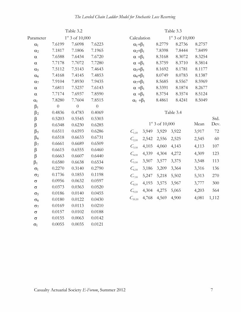
The Leveled Chain Ladder Model for Stochastic Loss Reserving
Casualty Actuarial Society E-Forum, Summer 2012 7
Table 3.2 Parameter 1st 3 of 10,000
α1 7.6199 7.6098 7.6223 … α2 7.1817 7.1806 7.1965 … α3 7.6588 7.6434 7.6720 … α4 7.7178 7.7072 7.7280 … α5 7.5112 7.5143 7.4643 … α6 7.4168 7.4145 7.4853 … α7 7.9104 7.8930 7.9435 … α8 7.6811 7.5237 7.6143 … α9 7.7174 7.6937 7.8590 … α10 7.8280 7.7604 7.8515 … β1 0 0 0 … β2 0.4836 0.4783 0.4069 … β3 0.5203 0.5545 0.5303 … β4 0.6348 0.6230 0.6285 … β5 0.6511 0.6593 0.6286 … β6 0.6518 0.6633 0.6731 … β7 0.6661 0.6689 0.6509 … β8 0.6615 0.6555 0.6460 … β9 0.6663 0.6607 0.6440 … β10 0.6580 0.6638 0.6534 … σ1 0.2270 0.3140 0.2790 … σ2 0.1736 0.1853 0.1198 … σ3 0.0956 0.0632 0.0597 … σ4 0.0373 0.0363 0.0520 … σ5 0.0186 0.0140 0.0455 … σ6 0.0180 0.0122 0.0430 … σ7 0.0169 0.0113 0.0210 … σ8 0.0157 0.0102 0.0188 … σ9 0.0155 0.0063 0.0142 … σ10 0.0055 0.0035 0.0121 …
Table 3.3 Calculation 1st 3 of 10,000
α1+β10 8.2779 8.2736 8.2757 … α2+β10 7.8398 7.8444 7.8499 … α3+β10 8.3168 8.3072 8.3254 … α4+β10 8.3759 8.3710 8.3814 … α5+β10 8.1692 8.1781 8.1177 … α6+β10 8.0749 8.0783 8.1387 … α7+β10 8.5685 8.5567 8.5969 … α8+β10 8.3391 8.1874 8.2677 … α9+β10 8.3754 8.3574 8.5124 … α10+β10 8.4861 8.4241 8.5049 …
Table 3.4
1st 3 of 10,000
Mean
Std. Dev.
C1,10 3,949 3,929 3,922 … 3,917 72 C2,10 2,542 2,556 2,525 … 2,545 60 C3,10 4,103 4,060 4,143 … 4,113 107 C4,10 4,339 4,304 4,272 … 4,309 123 C5,10 3,507 3,577 3,375 … 3,548 113 C6,10 3,186 3,209 3,364 … 3,316 136 C7,10 5,247 5,218 5,502 … 5,313 270 C8,10 4,193 3,575 3,967 … 3,777 300 C9,10 4,304 4,275 5,065 … 4,203 564 C10,10 4,768 4,569 4,900 … 4,081 1,112

The Leveled Chain Ladder Model for Stochastic Loss Reserving
Casualty Actuarial Society E-Forum, Summer 2012 8
4. COMPARISIONS WITH THE MACK MODEL
This section compares results obtained on the example above from Version 1 of the LCL models with those obtained from the Mack [3] model as implemented in the R “ChainLadder” package. A summary of these results are in Table 4.1.
Table 4.1
Leveled Chain Ladder – V1 Mack Chain Ladder w Estimate Std. Error CV Estimate Std. Error CV Actual 1 3,917 72 0.0184 3,917 0 0.0000 3,917 2 2,545 60 0.0236 2,538 0 0.0000 2,532 3 4,113 107 0.0260 4,167 3 0.0007 4,279 4 4,309 123 0.0285 4,367 37 0.0085 4,341 5 3,548 113 0.0318 3,597 34 0.0095 3,587 6 3,316 136 0.0410 3,236 40 0.0124 3,268 7 5,313 270 0.0508 5,358 146 0.0272 5,684 8 3,777 300 0.0794 3,765 225 0.0598 4,128 9 4,203 564 0.1342 4,013 412 0.1027 4,144 10 4,081 1,112 0.2725 3,955 878 0.2220 4,181
Total w=2,…,10 35,206 1,524 0.0433 34,997 1,057 0.0302 36,144
What follows is a series of remarks describing the construction of Table 4.1
• The estimates in both models represent the expected claims amounts for d = 10. • The LCL estimates and standard errors were calculated as described in Section 3 above. • The Mack [3] standard errors represent, as described in the ChainLadder package user
manual, “the total variability in the projection of future losses by the chain ladder method.”
• The Mack [3] standard error for w = 1 will, by definition, always be zero. Since the α1 and β10 parameters are estimates and hence have variability, the standard error for C1,10
given by the LCL models will be positive. How to make use of this feature (e.g., uncertainty in further development) might make for an interesting discussion, but since our goal is to predict {Cw,10}, I chose to omit consideration of the variability of C1,10 in any analyses of variability of the totals.
• The CAS Loss Reserve Database contains the completed triangles for the purpose of retrospective testing. The actual outcomes for {Cw,10} are included here for those who might be curious.

The Leveled Chain Ladder Model for Stochastic Loss Reserving
Casualty Actuarial Society E-Forum, Summer 2012 9
Figure 4.1 is a graphical representation of the information in Table 4.1.
Figure 4.1
The actual claims amounts points are connected by the line. The darker colored points slightly to the right of the “actual” points are the result of a sample of 100 simulated claims amounts taken from the LCL model. The lighter colored points slightly to the left of the “actual” points are from 100 simulations from a lognormal distribution matching the first two moments given by the Mack [3] model.
The simulated points from the Mack [3] model have smaller standard errors than the standard errors of simulated points from the LCL model. This is to be expected, since the LCL model has more “estimated” parameters. In inspecting other triangles I have found that this is almost always the case, as illustrated in Figure 4.2, where most of the standard errors of the Mack [3] model lie below the diagonal line that represents equality of the standard errors.
At least for this triangle, the span of the simulated points from both models contains the actual outcomes. But for some accident years, this is barely the case.
For the total claims amount over w going from 2 to 10, the actual total, 36,144, lies at the 76th percentile as measured by the LCL predictive distribution. It lies at the 86th percentile as measured by the Mack predictive distribution. The Mack predictive distribution was determined by fitting a lognormal distribution to the first two moments of the total estimate and standard error. Taken by themselves, these observations do not favor one model over the other. To measure the relative

The Leveled Chain Ladder Model for Stochastic Loss Reserving
Casualty Actuarial Society E-Forum, Summer 2012 10
performance of the models, we turn to fitting these models to a large number of triangles taken from the CAS Loss Reserve Database.
Figure 4.2

The Leveled Chain Ladder Model for Stochastic Loss Reserving
Casualty Actuarial Society E-Forum, Summer 2012 11
5. RETROSPECTIVE TESTS OF THE PREDICTIVE DISTRIBUTIONS
This section tests considers the LCL – Version 1 model that predict the distribution of unsettled claims using holdout data that is in the CAS Loss Reserve Database. As stated above, the model provides predictions for the sum of the losses {Cw,10} for w = 2, …,10 using {Cw,d} for w + d ≤ 11 as observations. The database contains the actual outcomes available for testing.
This paper’s goal is not to produce the smallest error. Instead it is to accurately predict the
distribution of outcomes. For a given sum of claims amounts, 10
,102
,ww
C=
∑ the model can calculate its
percentile. If the model is appropriate, the set of percentiles that are calculated over a large sample of insurers should be uniformly distributed. And this is testable.
The most intuitive test for uniformity is to simply plot a histogram of the percentiles and see if the percentiles “look” uniform. If given a set of percentiles {pi} for i = 1, , n, a more rigorous test would be to use PP plots. To do a PP plot, one first sorts the calculated percentiles, {pi}, in increasing order and plots them against the expected percentiles, i.e., the sequence {i/(n+1)}. If the model that produces the actual percentiles is appropriate, this plot should produce a straight line through the origin with slope one. In practice, the sorted percentiles will not lie exactly along the line due to random variation. But we can appeal to the Kolmogorov-Smirnov test. See, for example, Klugman [2] to account for the random variation. This test can be combined with the PP plot by
adding lines with slope one and intercepts ± 1.36/ n to form a 95% confidence band within which the points in the PP plots must lie.
This section shows the results of the above uniformity tests for both paid and incurred losses reported in Schedule P for four lines of insurance, Commercial Auto, Personal Auto, Workers Compensation and Other Liability. After filtering out bad data, I selected 50 insurers for each line of insurance from the CAS Loss Reserve Database. Appendix A lists the insurers selected and describes the filtering criteria.
The results of the uniformity tests are in Figures 5.1-5.10.

The Leveled Chain Ladder Model for Stochastic Loss Reserving
Casualty Actuarial Society E-Forum, Summer 2012 12
Figure 5.1

The Leveled Chain Ladder Model for Stochastic Loss Reserving
Casualty Actuarial Society E-Forum, Summer 2012 13
Figure 5.2

The Leveled Chain Ladder Model for Stochastic Loss Reserving
Casualty Actuarial Society E-Forum, Summer 2012 14
Figure 5.3

The Leveled Chain Ladder Model for Stochastic Loss Reserving
Casualty Actuarial Society E-Forum, Summer 2012 15
Figure 5.4

The Leveled Chain Ladder Model for Stochastic Loss Reserving
Casualty Actuarial Society E-Forum, Summer 2012 16
Figure 5.5

The Leveled Chain Ladder Model for Stochastic Loss Reserving
Casualty Actuarial Society E-Forum, Summer 2012 17
Figure 5.6

The Leveled Chain Ladder Model for Stochastic Loss Reserving
Casualty Actuarial Society E-Forum, Summer 2012 18
Figure 5.7
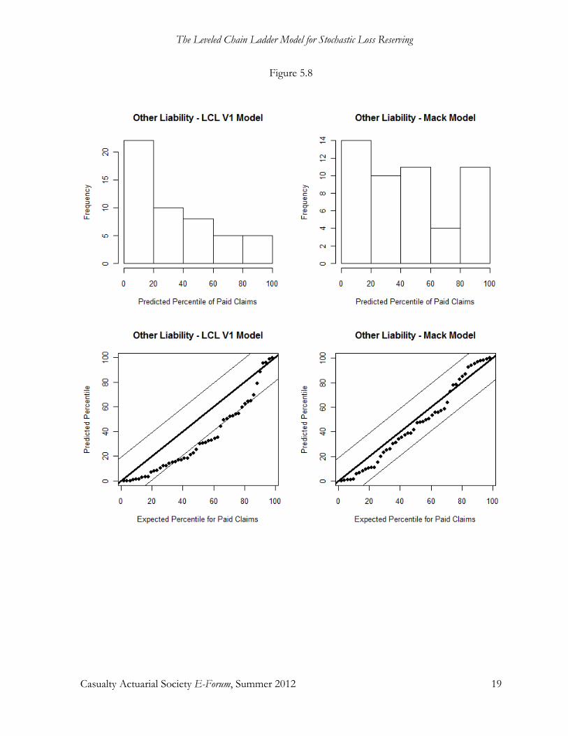
The Leveled Chain Ladder Model for Stochastic Loss Reserving
Casualty Actuarial Society E-Forum, Summer 2012 19
Figure 5.8

The Leveled Chain Ladder Model for Stochastic Loss Reserving
Casualty Actuarial Society E-Forum, Summer 2012 20
Figure 5.9

The Leveled Chain Ladder Model for Stochastic Loss Reserving
Casualty Actuarial Society E-Forum, Summer 2012 21
Figure 5.10

The Leveled Chain Ladder Model for Stochastic Loss Reserving
Casualty Actuarial Society E-Forum, Summer 2012 22
The results are mixed when looking at the individual lines of insurance for these incurred claims data. The PP-plots lie within the 95% confidence bands for three of the four lines for the LCL Version 1 model. They lie within two of the 95% confidence bands for the four lines for the Mack model. The results are less mixed for these paid claims data. The PP-plots lie within the 95% confidence bands for only the line “Other Liability” for the Mack model. The remaining PP-plots for paid claims data lie well outside the 95% confidence bands.
The picture become clearer when we combine the percentiles in all four lines, as is done in Figures 5.9 and 5.10. While outside the 95% confidence bands, the PP-plots for the incurred claims are close to the band, with the Version 1 model performing somewhat better than the Mack model. The histograms of the percentiles indicate that there are more outcomes than expected in both the high and the low percentiles, i.e., the ranges indicated by both models are too narrow. As indicated by Figure 4.2, the Version 1 model estimates of the standard error are higher than the Mack model estimates, so it should come as no surprise that the Version 1 model performs better than the Mack model on these incurred claims data.
The plots for these paid claims data indicate that neither model is appropriate. I consider that the most likely explanation is that the paid data is missing some important information, some of which is included in the incurred data.
6. CORRELATION BETWEEN ACCIDENT YEARS
One possible reason that the LCL Version 1 model produces ranges that are too narrow is that it fails to recognize that there may be positive correlation between claims payments between accident years. In this section I will propose a model that allows for such correlations, and test the predictions of this model on the holdout data.
To motivate this model, let’s suppose we are given random variables X and Y with means µX and µY with common standard deviation σ. If we set Y = µY + z·(X – µX) we can calculate the coefficient of correlation between X and Y as
( ) ( ) ( ) ⋅ − µ− µ ⋅ − µ ρ = = =σ σ
2
2 2
XX YE z XE X Y
z .
The proposed model will be one where the logarithms of the claims are correlated between successive accident years. We will refer this model as the LCLVersion 2 model.

The Leveled Chain Ladder Model for Stochastic Loss Reserving
Casualty Actuarial Society E-Forum, Summer 2012 23
( )( )( )
1, 1
, 1, 1
~ lognormal ,
~ lognormal , for = 2,...,
d d d
w d w d w d w d d
C
C z C w K− −
α + β σ
α + β + ⋅ − α −β σ (6.1)
Equation 6.1 in Version 2 replaces Equation 2.3 in Version 1. The coefficient of correlation, z, is treated as a random variable with its prior distribution being uniformly distributed between -1 and +1. All other assumptions in Version 2 remain the same as in Version 1. The Bayesian MCMC simulation in Version 2 proceeds pretty much the same as described in Section 3, with the sole difference being the presence of the additional parameter z. Here is a more detailed description of the simulation.
1. Similar to Table 3.2, the JAGS program returns 10,000 vectors {αw}, {βd}, {σd} and z. 2. Similar to Table 3.3, the R program calculates the mean logs
( )1, 1w d w d w dz C − −α + β + ⋅ − α −β .
3. Similar to Table 3.4, the R program simulates claims (sequentially in order of increasing w)
from a lognormal distribution with mean log ( )1, 1w d w d w dz C − −α + β + ⋅ − α −β and
standard deviation log σd.
While hypothesizing correlation between successive accident years, by choosing the prior distribution for z to be uniform between -1 and 1, this model does not force the correlation to be any particular value. If the correlation was spurious, the zs would cluster around zero. I ran the model on the data in Table 3.1. Figure 6.1 provides a histogram that strongly supports the presence of positive correlation. Table 6.1 shows that the predicted standard errors for Version 2 are significantly larger than those predicted by Version 1.
Tables 6.2 – 6.6 provide PP plots for Version 2 that are analogous to the Version 1 plots in Section 5. These plots show that the LCL Version 2 model percentile predictions lie within the bounds specified by the Kolmogorov-Smirnov test at the 95% level for incurred claims, but do not lie within the bounds for the paid claims.

The Leveled Chain Ladder Model for Stochastic Loss Reserving
Casualty Actuarial Society E-Forum, Summer 2012 24
Figure 6.1
Table 6.1
Leveled Chain Ladder V2 Leveled Chain Ladder V1
w Estimate Std. Error CV Estimate Std. Error CV Actual 1 3,918 86 0.0219 3,917 72 0.0184 3,917 2 2,546 74 0.0291 2,545 60 0.0236 2,532 3 4,113 135 0.0328 4,113 107 0.0260 4,279 4 4,324 162 0.0375 4,309 123 0.0285 4,341 5 3,565 154 0.0432 3,548 113 0.0318 3,587 6 3,338 179 0.0536 3,316 136 0.0410 3,268 7 5,237 356 0.0680 5,313 270 0.0508 5,684 8 3,736 377 0.1009 3,777 300 0.0794 4,128 9 4,122 699 0.1696 4,203 564 0.1342 4,144 10 3,937 1,367 0.3472 4,081 1,112 0.2725 4,181
Total w=2,…,10 34,918 2,192 0.0628 35,206 1,524 0.0433 36,144

The Leveled Chain Ladder Model for Stochastic Loss Reserving
Casualty Actuarial Society E-Forum, Summer 2012 25
Figure 6.2

The Leveled Chain Ladder Model for Stochastic Loss Reserving
Casualty Actuarial Society E-Forum, Summer 2012 26
Figure 6.3
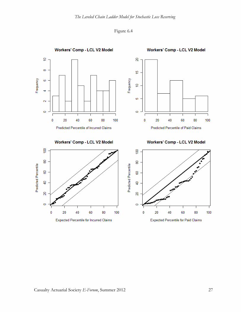
The Leveled Chain Ladder Model for Stochastic Loss Reserving
Casualty Actuarial Society E-Forum, Summer 2012 27
Figure 6.4

The Leveled Chain Ladder Model for Stochastic Loss Reserving
Casualty Actuarial Society E-Forum, Summer 2012 28
Figure 6.5

The Leveled Chain Ladder Model for Stochastic Loss Reserving
Casualty Actuarial Society E-Forum, Summer 2012 29
Figure 6.6

The Leveled Chain Ladder Model for Stochastic Loss Reserving
Casualty Actuarial Society E-Forum, Summer 2012 30
7. CONCLUDING REMARKS
When a model fails to validate on holdout data one has two options. First, one can improve the model. Second, one can search for additional information to include in the model. This paper is the result of an iterative process where one proposes a model, watches it fail, identifies the weaknesses, and proposes another model. Successful modeling requires both intuition and failure.
The successful validation of the LCL Version 2 model on the incurred claims data was preceded by the failure of a quite elaborate model, Meyers-Shi [6], built with paid incremental data. This led to the decision to try a model based on cumulative incurred claims, and continued through Versions 1 and 2 of the LCL model.4
The simultaneous successful validation of Version 2 on incurred claims and the failure of any model (that I tried) to validate with paid claims suggest that there is real information in the case reserves that cannot be ignored in claims reserving.
A key element in the success of the LCL model is its Bayesian methodology. The simulations done in Meyers [5] suggest that models with a large number of parameters fit by maximum likelihood will understate the variability of outcomes, and that a Bayesian analysis can, at least in theory, fix the problem. The recent developments in the Bayesian MCMC methodology make the Bayesian solution practical.
The LCL models were designed to work with Schedule P claims data. Individual insurers often have access to information that is not published in their financial statements. We should all recall that stochastic models produce conditional probabilities that are not valid in the presence of additional information.That being said, I suspect that many insurers will find the LCL model useful, as it reveals what the outside world could see.
To the best of my knowledge, no stochastic loss reserve model has ever been validated on such a large scale. In any modeling endeavor, the first is always the hardest. Now that we have some idea of what it takes to build a successfully validated model, I would not be surprised to see better models follow.
4There were numerous other modeling attempts that will remain unreported.

The Leveled Chain Ladder Model for Stochastic Loss Reserving
Casualty Actuarial Society E-Forum, Summer 2012 31
8. The R/JAGS CODE
The code that produced Tables 4.1 and 6.1 and Figure 4.1 is included in the CAS eForum along with this paper. The code is written in R (freely downloadable from www.r-project.org) and JAGS (freely downloadable from www.mcmc-jags.sourceforge.net). The code requires that the CAS Loss Reserve Database (www.casact.org/research/index.cfm?fa=loss_reserves_data) be downloaded and placed on the user’s computer. The code requires the use of the “rjags” and the “ChainLadder” packages in R.
The user should place the files “LCL1 Model.R,” “LCL2 Model.R,”“LCL1-JAGS.txt,” and “LCL2-JAGS.txt” into a working directory. In the first four lines of the R code the user should specify: (1) the name of the working directory; (2) the name and location of the file in the CAS Loss Reserve Database; (3) the group code for the insurer of interest; and (4) the type of loss – either paid or incurred. Then run the code. The code takes about a minute to complete and two progress bars indicate how much of the processing has completed.
The code should work for any complete 10 x 10 triangle. Similar code has run for all the group ids listed in Appendix A.

The Leveled Chain Ladder Model for Stochastic Loss Reserving
Casualty Actuarial Society E-Forum, Summer 2012 32
APPENDIX A – GROUP CODES FOR SELECTED INSURERS
Commercial Personal Workers’ Other Auto Auto Comp Liab 353 353 86 620 388 388 337 671 620 620 353 683 671 671 388 715 833 715 671 833 1066 965 715 1066 1090 1066 1066 1090 1538 1090 1252 1252 1767 1538 1538 1538 2003 1767 1767 1767 2135 2003 2135 2003 2208 2143 2712 2135 2623 3240 3034 2143 2712 4839 3240 2208 3240 5185 5185 2348 3492 5320 6408 3240 4839 5690 7080 5185 5185 6947 8559 5320 5320 8427 9466 6408 6408 8559 10385 6459 6459 10022 10699 6807 6777 11037 11126 6947 6947 11126 11347 8079 7080 13420 11703 10657 8427 13439 13439 11118
Commercial Personal Workers’ Other Auto Auto Comp Liab 8559 13501 13501 11126 10022 13641 13528 11460 10308 13889 14176 12866 11037 14044 14257 13501 11118 14257 14320 13641 13439 14311 14370 13919 13641 14443 14508 14044 13889 15199 14974 14176 14044 15407 15148 14257 14176 15660 15199 14370 14257 16373 15334 14974 14320 16799 16446 15024 14974 18163 18309 15571 18163 18791 18767 16446 18767 23574 18791 18163 19020 25275 21172 18686 21270 25755 23108 18767 26077 27022 23140 26797 26433 27065 26433 27065 26905 29440 27529 28436 27065 31550 34576 35408 29440 34509 37370 37052 31550 34592 38687 38733 37036 35408 38733 41459 38733 42749 41300 41580
Selection Criteria
1. Removed all insurers with incomplete 10 x 10 triangles. 2. Sorted insurers in order of the coefficient of variation of the premium. 3. Visually inspected insurers and removed those (very few) with “funny behavior.” 4. Kept the top 50.

The Leveled Chain Ladder Model for Stochastic Loss Reserving
Casualty Actuarial Society E-Forum, Summer 2012 33
REFERENCES
[1] England, P.D., and R.J. Verrall, “Stochastic Claims Reservingin General Insurance,” Institute of Actuaries and Faculty of Actuaries, 28 January 2002.
[2] Klugman, Stuart A., Harry H. Panjer, and Gordon E. Willmot, Loss Models, From Data to Decisions, Second Edition, Wiley Series in Probability and Statistics, 2004.
[3] Mack, T., “Measuring the Variability of Chain Ladder Reserve Estimates,” Casualty Actuarial Society Forum, Spring 1994.
[4] Mack, Thomas, “Which Stochastic Model is Underlying the Chain Ladder Method?”,Casualty Actuarial Society Forum, Fall 1995.
[5] Meyers, Glenn G., “Thinking Outside the Triangle,” ASTIN Colloquium, 2007 [6] Meyers, Glenn G. and Peng Shi, “The Retrospective Testing of Stochastic Loss Reserve Models,”Casualty
Actuarial Society E‐Forum, Summer 2011. [7] Meyers, Glenn G., “Quantifying Uncertainty in Trend Estimates with JAGS,” The Actuarial Review, Vol. 39,
No. 2. May 2012. [8] Taylor, G. C.,Claims Reserving In Non-Life Insurance,Elsevier Science Publishing Company, Inc., 1986.
Biography of the Author
Having worked as an actuary for over 37 years, Glenn Meyers retired at the end of 2011. His last 23 years of employment were spent working as a research actuary for ISO. In retirement, he still spends some of his time pursuing his continuing passion for actuarial research.

Casualty Actuarial Society E-Forum, Summer 2012 1
A Practical Way to Estimate One-year Reserve Risk
Ira Robbin, PhD ______________________________________________________________________________ Abstract
The advent of Solvency II has sparked interest in methods for estimating one-year reserve risk. This paper provides a discussion of the one-year view of reserve risk and some of the methods that have been proposed for quantifying it. It then presents a new method that uses ultimate reserve risk estimates, payment patterns, and reporting patterns to derive one-year reserve risk values in a systematic fashion. The proposed method is a more refined version of the simplistic approach used in the Standard Formula. Yet, it is also practical and robust: triangles, regressions, or simulations are not required. Keywords: Solvency II, One-year Reserve Risk, Best Estimate, Loss Reserves, Technical Provision.
______________________________________________________________________________
Table of Contents
A PRACTICAL WAY TO ESTIMATE ONE-YEAR RESERVE RISK ................................. 1
1. INTRODUCTION ................................................................................................................... 2
2. ONE-YEAR RESERVE RISK ............................................................................................... 4 2.1 One-year Reserve Risk Illustrative Example .................................................................................. 4 2.2 Conceptual Drivers of One-year Reserve Risk .............................................................................. 5
2.2.1 Long-Tailed Lines ......................................................................................................................................... 5
3. SOLVENCY II TECHNICAL PROVISION CALCULATION ..................................... 6
4. STANDARD FORMULA RESERVE CAPITAL .............................................................. 6 4.1 Standard Formula Premium and Reserve Risk .............................................................................. 7 4.2 CVs and Risk Margins by LOB ........................................................................................................ 7 4.3 Size Independent Formula ................................................................................................................ 8 4.4 Standard Formula Calibration to Average Size Portfolio ............................................................ 8
5. ONE-YEAR RESERVE RISK DATA ................................................................................. 9 5.1 Schedule P One-year Reserve Tests ................................................................................................ 9 5.2 Ranges .................................................................................................................................................. 9
6. ONE- YEAR RESERVE RISK FROM AN INTERNAL MODEL ............................ 10 6.1 Size Dependence and Modeling Refinements ............................................................................. 10 6.2 One-year Reserve Risk Estimation Methods ............................................................................... 11
6.2.1 One-year Variance in Chain Ladder Projection Ultimate .................................................................... 11 6.2.2 Triangle Regression Analysis .................................................................................................................... 12 6.2.3 Simulation of Next Diagonal and Actuary-in-a-Box Revaluation ...................................................... 13 6.2.4 Bootstrapping and Extended Simulation Results .................................................................................. 13 6.2.5 Recognition Factor Methods .................................................................................................................... 14
6.3 Comparative Summary of One-year Reserve Risk Methods ..................................................... 15
7. PROPOSED FORMULA ...................................................................................................... 16 7.1 CV for Ultimate Unpaid .................................................................................................................. 17

A Practical Way to Estimate One-year Reserve Risk
Casualty Actuarial Society E-Forum, Summer 2012 2
7.2 CV of Case Reserves vs. IBNR ..................................................................................................... 17 7.3 Projected Evolution of Case O/S and IBNR .............................................................................. 19 7.4 Projecting Ultimate Risk by Year ................................................................................................... 24 7.5 From Ultimate Risk to One-year Risk........................................................................................... 25 7.6 Discounted SCR and Technical Provision ................................................................................... 28
8. CONCLUSION ....................................................................................................................... 30
APPENDIX A –LOGNORMAL STANDARD FORMULA CALCULATIONS ............... 30
APPENDIX B –ONE-YEAR RESERVE RISK FORMULAS AND DERIVATIONS .... 31
REFERENCES.................................................................................................................................. 34
1. INTRODUCTION
One-year reserve risk is a relatively new concept, especially for actuaries in the United States. Historically, actuaries have been concerned with whether the reserve is adequate to cover ultimate loss. With the advent of Solvency II, actuaries have now also begun to consider the one-year perspective. Under Solvency II, the capital requirement for unpaid loss is defined as the amount sufficient to cover risk over a single year. Solvency II also features a market-consistent approach to the valuation of unpaid loss liabilities.1
What is one-year reserve risk and how is it computed? Conceptually, it is a measure of how much an initial unbiased mean estimate of the reserve might change in one year. Under European Insurance and Occupational Pensions Authority (EIOPA) regulations, such risk can be computed either with a carefully delineated Standard Formula or, alternatively, with an approved, enterprise-specific internal model.
Under this approach to valuation, unbiased estimates of unpaid loss are discounted and then loaded with an explicit risk margin. This risk margin depends on the projected capital requirements over the run-off period. So, under Solvency II, one-year risk dictates not only the capital requirement, but also the valuation of the reserve.
2
The Standard Formula assumes a lognormal distribution of one-year retrospective results for each EIOPA line of business. Each line is assigned a single coefficient of variation (CV) that applies
1 There is no market in which loss liabilities are openly traded. So the market-based approach is really a mark-to-model approach. Not enough is disclosed about loss portfolio transfers to fit pricing on these deals to a model. 2 Partial use of an internal model is also allowed subject to regulatory approval.

A Practical Way to Estimate One-year Reserve Risk
Casualty Actuarial Society E-Forum, Summer 2012 3
to all its unpaid losses and to each year of run-off. The CVs are promulgated by EIOPA.3
An internal model tailored to the business written by a company should provide a more accurate estimate of its capital requirement. Yet, a firm may be reluctant to use an internal model. Building such a model is costly. The model must be supported by extensive documentation and it must pass validation checks. It must clear imposing regulatory hurdles. After all that, the model might well show the firm needs more capital than would be indicated by the Standard Formula.
The regulator also mandates a correlation matrix and prescribes algorithmic procedures for arriving at the all-lines aggregated estimate of one-year reserve risk.
4
Even with an internal model, a company must still derive the required reserve capital based on one-year reserve risk. Several authors have presented methods for deriving one-year reserve risk.
5
The paper will first provide an intuitive explanation of one-year reserve risk and outline the key conceptual factors that determine its magnitude. Then there will be a brief overview of how one-year reserve risk is used in computing Solvency II Solvency Capital Requirements (SCR) and the related Risk Margins in the Technical Provision for unpaid loss. Following that, the paper will summarize how one-year reserve risk is quantified in the Standard Formula. Next there will be discussion of the challenges faced in using Schedule P reserve tests or reserve ranges to derive Solvency II consistent one-year reserve risk values. Then, the paper will survey various methods that have been proposed to quantify one-year reserve risk in an internal model context. The paper will examine some of the difficulties in implementing such models and applying them to long-tailed lines of business with sparse data.
This paper provides another technique. It is a bit more sophisticated than the Standard Formula, while being more practical and robust than many of the other proposed internal model approaches.
This will lead to a presentation of the proposed algorithm. It is very similar to the Standard Formula in that it uses lognormal distributions and CVs. Yet, it has two key features that distinguish it from the Standard Formula. First, it employs systematically derived CVs that vary based on the decomposition of the unpaid loss between IBNR and Case Outstanding (Case O/S)
3 In December 2011, the Joint Working Group (JWG)[5] recommended revisions in the proposed factors based on its calibration analysis. 4 It is unclear whether Solvency II will increase or decrease in required funds relating to unpaid losses For long-tailed lines, the one-year view of risk may tend to produce a fairly small capital requirement, even if the ultimate risk is quite large. Discounting with an illiquidity premium, as dictated by Solvency II, also reduces the funds backing the unpaid loss liability. 5 See Merz and Wuthrich [8], Ohlsson and Lauzeningks [10], and Rehmann and Klugman [11].

A Practical Way to Estimate One-year Reserve Risk
Casualty Actuarial Society E-Forum, Summer 2012 4
reserves. This leads to CVs that may change each year as the reserve runs off. Depending on the expected evolution of the mix of unpaid loss, the “Varying CV” model being proposed in this paper could arrive at capital requirements and risk margins higher or lower than the Standard Formula. The other key feature of the proposed algorithm is that it uses the expected change in ultimate reserve risk in order to derive one-year reserve risk. This is a natural approach that automatically reconciles ultimate reserve risk with the series of one-year views.
2. ONE-YEAR RESERVE RISK
What is one-year reserve risk? Intuitively, it is a gauge of how much the estimated ultimate loss might change over one year. Conceptually, it is equivalent to the variability in estimates of ultimate loss made one year later. In the context of Solvency II, the expected unpaid loss is called the undiscounted Best Estimate and it is assumed to be unbiased and have no built-in prudential margin. To restate with a bit more precision, one-year reserve risk is an assessment made at the current evaluation date of the variability that could exist in retrospective Best Estimate reserve valuations made one year later.
2.1 One-year Reserve Risk Illustrative Example To clarify the concept, assume the set of scenarios and probabilities shown in Table 1. At the
initial evaluation date, there is no way of knowing which scenario holds. What is known is that the mean unpaid is $100 over the four scenarios. Thus $100 is the initial undiscounted Best Estimate.
Table 1
( 1 ) ( 2 ) ( 3 ) ( 4 ) ( 5 ) ( 6 ) ( 7 ) ( 8 ) ( 9 ) ( 10 )
Scenario Prob
Initial Case O/S
Initial IBNR
Initial Estimate Unpaid
Yr 1 Paid
End of Yr 1 Case O/S
End of Yr 1IBNR
End of Yr 1 Est'd Unpaid
Retro Estimate Intial Unpaid
(3) + (4) (7) + (8) (6) + (9)1 25% $40 $60 $100 $10 $45 $40 $85 $952 25% $40 $60 $100 $10 $30 $35 $65 $753 25% $40 $60 $100 $30 $45 $50 $95 $1254 25% $40 $60 $100 $30 $30 $45 $75 $105
Avg $40 $60 $100 $20 $38 $43 $80 $100Stnd Dev $18

A Practical Way to Estimate One-year Reserve Risk
Casualty Actuarial Society E-Forum, Summer 2012 5
In each scenario, a retrospective (retro) estimate of the initial unpaid is obtained by adding the year one paid amount to the estimate of mean unpaid loss as of the end of year one. One-year reserve risk arises from the volatility of these retro estimates. The $18 standard deviation of the retro estimates is a quantification of the one-year reserve risk.
The example highlights the importance of the information to be gained over one year and the yearly movement in the distribution of the estimates of unpaid loss. It also demonstrates the importance of IBNR estimation. In this example, the calculation of the IBNR has been left deliberately vague. A different IBNR calculation might have produced IBNR estimates different from the ones shown in Column 8 of Table 1 and thus led to a different standard deviation value.
2.2 Conceptual Drivers of One-year Reserve Risk There are three conceptual drivers of one-year reserve risk.
• First is the inherent volatility of the ultimate unpaid loss. Both the amount and timing will in general differ from current mean estimates. The difference can be due to random statistical fluctuation, systematic movement in underlying claims processes, and inherent estimation error in the initial undiscounted Best Estimate.
• Second is the amount of information that will be gained over one year. This information could include claim data such as paid loss, reported loss, claims closed, claims reported, and so forth, as well as external information such as a new judicial ruling or a medical treatment that could influence subsequent claims settlements. The information we gain is subject to statistical fluctuations.
• Third is the methodology and data used to derive an updated Best Estimate one year later. Actuaries often work up indications with a variety of methods and data. They may have a set of default weights for averaging the methods to get a final pick. Such weights would usually vary by accident year maturity.
2.2.1 Long-Tailed Lines
When reserving long-tailed lines, actuaries generally opt for stability over responsiveness, at least for the first few years of development. This is entirely appropriate: wild swings in the valuation of reserves would justifiably undermine confidence in such valuations. However, one consequence is that long-tailed lines with the largest reserve risk at ultimate might have one-year reserve risk values that are relatively small in magnitude. It has been noted that the overall conceptual basis of one-year

A Practical Way to Estimate One-year Reserve Risk
Casualty Actuarial Society E-Forum, Summer 2012 6
reserve risk could lead to a relatively low capital requirement for long-tail business, especially over the first few years of development.6
3. SOLVENCY II TECHNICAL PROVISION CALCULATION
The Solvency II Technical Provision (TP) as detailed in [4] is the sum of the Best Estimate (BE) plus a Risk Margin (RM).
𝑇𝑇𝑇𝑇= 𝐵𝐵𝐵𝐵+ 𝑅𝑅𝑅𝑅 (3.1)
By definition under Solvency II, the “Best Estimate” is the discounted mean of possible scenarios.7 The discounting is done using risk-free yield curves by currency as promulgated by EIOPA. The rates used for discounting are increased by “illiquidity” premiums that are also promulgated by EIOPA.8
𝐵𝐵𝐵𝐵= 𝐵𝐵[𝑇𝑇𝑃𝑃 𝑜𝑜𝑜𝑜 𝑈𝑈𝑈𝑈𝑈𝑈𝑈𝑈𝑈𝑈𝑈𝑈 𝐿𝐿𝑜𝑜𝐿𝐿𝐿𝐿]
(3.2)
The Risk Margin is the present value of Cost of Capital charges for the projected Reserve Solvency Capital Requirements (SCRs) over the run-off period.9
𝑅𝑅𝑈𝑈𝐿𝐿𝑅𝑅 𝑅𝑅𝑈𝑈𝑀𝑀𝑀𝑀𝑈𝑈𝑈𝑈= � 𝑀𝑀𝐶𝐶𝐶𝐶𝐶𝐶∙𝑆𝑆𝐶𝐶𝑅𝑅𝑦𝑦 ∙𝑣𝑣(𝑦𝑦)𝑦𝑦−1
(3.3)
Here rCOC is the required cost-of-capital rate10
The SCR each year is defined as the one-year reserve risk for that year. Thus computing the Technical Provision requires the actuary to project the series of one-year reserve risk values, year-by-year, over the run-off period.
and v(y) is the discount factor for year y.
4. STANDARD FORMULA RESERVE CAPITAL
Under EIOPA regulation [4], there are ten non-life Lines of Business (LOB). An SCR is
6 Ohlsson and Lauzeningks[10] observe, “ … a problem with the one-year is that reserves for long tail business might …require less solvency capital than some short tail business…. This is a general problem with the one-year horizon”. 7 Most property and casualty actuaries find this terminology confusing and inconsistent with common usage in the profession. One, England [6], memorably noted the need to “retune your mind” in connection with the Best Estimate definition. As needed for clarity we will refer to Undiscounted Best Estimates and Discounted Best Estimates. 8 Objections have been raised by property and casualty actuaries (See Schmidt [12]) to the use of Illiquidity Premiums. The effect of an Illiquidity Premium is to reduce the Best Estimate below the risk-free present value of unpaid loss. While Illiquidity Premiums may be used to explain market pricing of different investment instruments, there is no market of insurance liabilities with pricing data to validate whether this concept applies to property and casualty insurance liabilities. 9 See SCR 9.2 in [4]. 10 Currently set by EIOPA at 6.0%.

A Practical Way to Estimate One-year Reserve Risk
Casualty Actuarial Society E-Forum, Summer 2012 7
computed for the combination of Premium Risk and Reserve Risk for the aggregated LOBs.
4.1 Standard Formula Premium and Reserve Risk Under the Standard Formula, one-year reserve risk for each LOB is determined using a
lognormal distribution with a CV as mandated by EIOPA. A lognormal assumption and a CV are also provided for Premium Risk for each LOB. Formulas are used to define Premium Volume and Reserve Volume measures. A Premium-Reserve covariance assumption is used along with these volume measures to arrive at a CV and a volume measure for the combined premium and reserve risk. This is done for each LOB. A combined lines CV is then derived using a correlation matrix supplied by EIOPA along with the individual LOB CVs and volume measures. An overall volume measure is also computed. This is done with a formula that gives credit for geographical diversity.11
4.2 CVs and Risk Margins by LOB
The SCR for premium and reserve risk is computed by multiplying the volume measure against the 99.5% percentile excess of the mean. The overall SCR is then used to generate the cost-of-capital and the overall risk margin. This extremely brief overview is intended to give the reader a general introduction to the Standard Formula reserve risk algorithm. This provides the context for understanding the computation of the standalone reserve SCRs.
To allocate the overall risk margin by line, standalone SCRs at the LOB level are computed using the CVs provided by EIOPA. Then the guidance states, “The allocation of the risk margin to the lines of business should be done according to the contribution of the lines of business to the overall SCR during the lifetime of the business.”12
The original one-year CVs provided by EIOPA vary by LOB in a reasonable fashion as do the latest set of recalibrated factors produced by the JWG [5]. However, the use of one CV per line over the whole run-off period is a notable simplifying assumption. As reserves move from IBNR to a mix of IBNR and Case Outstanding and then to just Case Outstanding, it is not likely that the CV of the one-year development distribution would remain unchanged. However, the use of a single factor for each LOB is not uncommon in reserve capital requirement calculations. Rating
In Appendix A, we provide the derivation of a standalone SCR for reserves assuming the one-year distribution is lognormal as is done under the Standard Formula.
11 See SCR.9.2 in the QIS5 Technical Specifications [4] for more detail. 12 See TP.5.26 in the QIS5 Technical Specifications [4].

A Practical Way to Estimate One-year Reserve Risk
Casualty Actuarial Society E-Forum, Summer 2012 8
agency reserve capital formulas typically use a single factor for each line of business, irrespective of the mix of reserves or the age of development. Perhaps the key advantage of a “one factor per line” approach is that it makes the calculations tractable. Further, if appropriately calibrated, it should yield reasonable indications for a company with an established book of business that has maintained an average pattern of growth over time.
4.3 Size Independent Formula The Reserve SCR under the Solvency II Standard Formula is implicitly based on the assumption
that all risk is parameter risk. This follows because the formula does not reflect the size of the reserve.
A size independent method is certainly practical and convenient. It dispels issues of fairness between large and small companies. Size independent methods have been used and are being used in other capital requirement calculations. In particular, rating agency capital requirements for reserves are also typically computed by applying factors to the line of business reserve balances. The factors typically do not depend on the volume of reserves.
While convenience and consistency are advantages in using a fixed factor, size independent approach, such an approach implicitly ignores process risk. Ignoring process risk is the only way the same factor can be used for all companies, large and small. Yet, the actual risk for any given company includes both process and parameter risk. Depending on the type of business, volume of business, and the limits involved, either parameter or process risk may predominate. With a large volume of high frequency-low severity business, process risk will approach zero. On the other hand, process risk can be huge for a relatively small volume of low frequency-high severity business.
4.4 Standard Formula Calibration to Average Size Portfolio In calibrating factors for the Standard Formula, analysts have had to sidestep the contradiction in
using a size-independent formula to model a type of risk that is partly size dependent. The latest EIOPA JWG report on calibration [5] noted, “… volatility factors for premium and reserve risks are typically impacted by the size of the portfolio (in the sense that with increasing size the volatility will typically decrease). However, the JWG was mandated to derive single factors for each of the individual lines of business (separately for premium and reserve risk), irrespective of portfolio size since this is consistent with the current design of the standard formula approach”. The recommended factors are based on a portfolio of average size. The JWG recognized that any fixed factor “… will imply that the SCR will be too large for the larger portfolios and too small for the

A Practical Way to Estimate One-year Reserve Risk
Casualty Actuarial Society E-Forum, Summer 2012 9
smaller ones”.
5. ONE-YEAR RESERVE RISK DATA
Data from various countries and regulatory accounting paradigms have been examined by analysts [5] in deriving factors for the Solvency II Standard Formula. For possible use in internal models, we will briefly examine two sources of reserve volatility data that U.S. actuaries are familiar with.
5.1 Schedule P One-year Reserve Tests In the United States, the one-year reserve test in the NAIC Statutory Annual Statement is a
retrospective comparison providing information about current estimates of the adequacy of Booked Reserves one year ago. Results are shown by Schedule P line and by accident year. The one-year test would, in principle, provide an empirical measurement of undiscounted one-year reserve risk.
The problem is that Booked Reserves are not necessarily Best Estimates. Further, there may not be enough information disclosed to directly derive a Best Estimate. The Booked Reserves may include an implicit prudential margin. They may also be discounted at an undisclosed rate. As well, the adequacy of booked IBNR may vary over the underwriting cycle as companies build up and deplete reserve cushions in order to manage calendar year results.13 If that is the case, it may be effectively impossible to disentangle inherently random statistical and projection error from systemic non-random error due to cycle management of the booked reserves.14
5.2 Ranges
This could also partly explain high correlations between different lines of business. Solvency II measures risk with respect to the one-year change in the mean estimate of ultimate. If posted estimates of ultimate are not equal to the mean, one could argue that risk estimates derived from posted reserve data might systematically overstate or understate the “true” amount of Solvency II risk.
Actuaries in the United States have some considerable experience in estimating ranges for ultimate unpaid loss. The prior version of the relevant Actuarial Standard of Practice required an opining actuary to have such a range when judging whether a reserve was adequate, deficient, or
13 See Boor [2]. 14 In calibrating Standard Formula risk factors, the EIOPA JWG [5] noted “the possible existence of an underwriting cycle but did not find it practicable to incorporate or embed an explicit recognition of such cycles into the calibration methodology.”

A Practical Way to Estimate One-year Reserve Risk
Casualty Actuarial Society E-Forum, Summer 2012 10
redundant.15
Several problems need to be solved in order to use ranges to derive one-year reserve risk values. First an assumption is needed about how to translate a reserve range into a statement about statistics of the ultimate unpaid loss random variable. Sometimes, ranges are derived by looking at the range of estimates resulting from different reserving methodologies or different sets of parameters. For Solvency II applications the reserve range needs to be related to statistics of the unpaid loss distribution. For example, the range might be defined as two standard deviations under and over the mean or it might be the interval from the 25th percentile to the 75th percentile. Even after the range is related to a statement about the statistics of the ultimate loss random variable, additional significant assumptions may be needed to arrive at the 99.5% percentile. One common assumption, for instance, is that the distribution is lognormal. The next major problem is to figure out how to use the ultimate view to derive the series of one-year views. The variability at ultimate should lead to variability in the series of annual results over the run-off period. Volatility in the estimation process may add additional year-by-year movement. Another key challenge is practical: how to produce a consistent set of ranges in fine enough detail. Depending on the level of detail in an internal model, ranges might be needed by line, business unit, or by accident year. Usually ranges are not produced at such a level. Even if an actuary has a method for producing ranges at a high level of aggregation, an approach is needed to ensure ranges at a more granular level are consistent.
6. ONE- YEAR RESERVE RISK FROM AN INTERNAL MODEL
Solvency II regulations allow for partial or complete use of an internal model, subject to approval by supervisory authorities. Our focus is on use of an internal model to quantify one-year reserve risk. With an internal model, a firm may cut data in categories different those proscribed under the Standard Formula. It may also employ algorithms different from those used in the Standard Formula.
6.1 Size Dependence and Modeling Refinements An internal model may allow for consideration of process and parameter risk and it may be
implicitly or explicitly dependent on the volume of reserves. For large companies this may legitimately produce a relative capital requirement lower than that produced by the Standard Formula. 15 Under the latest ASOP #43 [1], ranges are not required if an actuary judges the reserves to be adequate.

A Practical Way to Estimate One-year Reserve Risk
Casualty Actuarial Society E-Forum, Summer 2012 11
An internal model might incorporate finer line of business breakouts than the Solvency II defaults. Such finer breakouts should result in a model that more closely matches the actual organizational and line of business divisions of a company. This is important if the internal model is ever to be employed for anything beyond computing regulatory capital requirements. Other uses need to be found if an internal model is to pass the “Use Test,” a requirement for approval of under Solvency II.16
An internal model can also reflect different levels of risk by accident year within a particular line of business. As was true for line of business refinement, accident year refinement should provide a more accurate model of the Best Estimate reserves.
With each refinement, the size of individual reserve cells gets smaller. A size-dependent internal model would assign each cell a relatively larger amount of process risk. However, after being added together, the aggregated result may have a lower amount of risk than if it had been left as an undivided whole. It all depends on the correlation assumptions.
6.2 One-year Reserve Risk Estimation Methods Several general ways have been proposed for estimating one-year reserve risk.
6.2.1 One-year Variance in Chain Ladder Projection Ultimate
Merz and Wuthrich [8] derive estimates for the variance in the one-year claims result17
However, the method does not directly generate the 99.5% percentile needed for Solvency II
based on the Distribution-Free Chain-Ladder framework. They built on work done by Mack on estimating variance at ultimate in projections made with the Chain-Ladder method. A key assumption is that unbiased estimates of ultimate losses can be obtained by applying age-to-latest age factors to the latest diagonal of cumulative paid losses. The age-to-latest age factors are derived from the triangle of paid loss data. Merz and Wuthrich arrive at closed-form estimators of the one-year prediction error with terms that depend only on the actual triangle of data. This work was ground-breaking and showed that results from a one-year perspective could be obtained with a standard reserving methodology.
16 Since an internal model is inappropriate or too cumbersome for either pricing business or estimating unpaid losses, the Use Test may be difficult to pass. Evaluating capital required for different business units may be a “use”, but that would vanish if the internal model is not done at the business unit level. 17 The one-year claims result is defined by Merz and Wuthrich as the difference between the retrospective estimate and the initial estimate of unpaid loss.

A Practical Way to Estimate One-year Reserve Risk
Casualty Actuarial Society E-Forum, Summer 2012 12
calculations. An additional assumption is needed. For example, as is often done in Standard Formula derivations, one could assume the distribution is lognormal. With the variance the method does generate and a lognormal assumption for the one-year claims result, the computation is straightforward. Another serious concern is that the method does not handle tail factors. Therefore it may not work on very long-tailed lines. In addition, it does not readily generalize beyond the Chain-Ladder framework.
6.2.2 Triangle Regression Analysis
Rehman and Klugman [11] analyze triangles of estimated ultimate losses. They assume the age-to-age ratios of the estimated ultimates are lognormal. They define the natural logs of the ratios as error random variables, 𝑒𝑒𝑈𝑈
𝑗𝑗 = ln(𝑈𝑈𝑈𝑈𝑗𝑗+1/𝑈𝑈𝑈𝑈
𝑗𝑗 ) where 𝑈𝑈𝑈𝑈𝑗𝑗 is the estimate of ultimate for accident year,
i, as of calendar year j. The development year is d = j- i +1. Under the lognormal assumption and assuming the lognormal parameters depend only on the development period (column), it follows that 𝑒𝑒𝑈𝑈
𝑗𝑗~𝑁𝑁(𝜇𝜇𝑈𝑈 ,𝜎𝜎𝑈𝑈2) . If an estimator is unbiased, one would have: 𝐵𝐵�𝑈𝑈𝑈𝑈𝑗𝑗+1/𝑈𝑈𝑈𝑈
𝑗𝑗 � = 1. For an unbiased estimator it would follow that 𝜇𝜇𝑈𝑈 = −.5 ∗ 𝜎𝜎𝑈𝑈2 . However, the method does not require the estimators be unbiased. The “µ” parameters are estimated by taking the average of error random variables in a column. The “σ” parameters are estimated by computing the sample variance (with bias adjusted denominator) in a column. Using the lognormal assumption one can compute the 99.5% percentile of the one-year error distribution as is needed for Solvency II. Rehman and Klugman [11] also compute overall error for an accident year and for a calendar year diagonal using empirical covariance estimates from the triangle.
The method of Rehman and Klugman is an analysis of results produced by an algorithm, but it does not require that the algorithm be specified. Of course, it is required that the same algorithm be used throughout the historical triangle and it is assumed the same algorithm will be used for the projection. Because it does not require the analyst to know just what algorithm is being used and because it is focused solely on the results that have been obtained, the methodology can be fairly described as a general and solidly empirical approach.18
Miccolis and Heppen [9] applied this approach to data from a number of insurance groups and
However the method does require as many evaluations as are needed for at least a few years to be fully developed. Otherwise the later evaluation age parameters may be very erratic.
18 As was noted by Rehman and Klugman [11], it can even be applied to paid or reported data as well as to the projected ultimates.

A Practical Way to Estimate One-year Reserve Risk
Casualty Actuarial Society E-Forum, Summer 2012 13
obtained good results for most lines. However, they noted problems could arise when data was sparse or subdivided into small business units. They suggested combining data for variance analysis.
6.2.3 Simulation of Next Diagonal and Actuary-in-a-Box Revaluation
Ohlsson and Lauzeningks [10] outline a simulation methodology that starts with an estimated unpaid amount that is assumed to be the actuary’s undiscounted Best Estimate. They further assume it is derived from a specified algorithm. This algorithm does not need to be a simple formula. It may encompass use of different particular methods that can vary by accident year maturity.19 The reserve computation algorithm is called the “actuary-in-a-box”.20
While the Ohlsson and Lauzeningks framework makes sense as a constructive way to estimate one-year reserve risk based on given assumptions supplied by the modeler, the user needs to be aware that the answer is based on those underlying assumptions.
Under the Ohlsson and Lauzeningks framework, a simulation model is then used to generate the next diagonal. Ohlsson and Lauzeningks did not specify distributional assumptions or forms: they left that to the modeler. All the simulation needs to do is to produce what the actuary-in-a-box requires to arrive at the updated Best Estimate. Then the model computes the retrospective Best Estimate of the initial unpaid. After running the simulation thousands of times, one will obtain a simulated distribution of one-year claim development results and the 99.5% percentile of this distribution is the initial capital requirement. This is a very general framework. By embedding it within a simulation model context, it allows the developer of an internal model to simulate correlations between accident years and between lines of business.
6.2.4 Bootstrapping and Extended Simulation Results
Boumezoued, Angoua, Devineau, and Boisseau [3] describe various general models within the simulation framework. One of particular interest is a bootstrapping simulation method that yields one-year (expected) simulated variance equal to the Merz and Wuthrich variance formula. However, their simulation does more than provide a way to approximate the variance. It also provides a direct way to estimate the 99.5% percentile.21 Boumezoued, Angoua, Devineau, and Boisseau also extend the one-year recursive bootstrap method to include a tail factor.22
19 Ohlsson and Lauzeningks mention for example a development factor and regression extrapolation method for older years and Generalized Cape Cod for the latest years.
20 The phrase “actuary-in-a-box” has been attributed to Ohlsson. 21 One could make a lognormal assumption and use the variance computed via the method of Merz and Wutrich to derive the CV. With the CV, one could then calculate the 99.5% percentile. 22 Recall the Merz and Wuthrich algorithm does not explicitly contemplate a tail factor.

A Practical Way to Estimate One-year Reserve Risk
Casualty Actuarial Society E-Forum, Summer 2012 14
Boumezoued, Angoua, Devineau, and Boisseau also analyze process error and perform simulations using different copulas to capture dependence between different accident years and lines of business. In addition, they compute the distribution for each year of the run-off period until ultimate. This set of computations for each of the years is needed for the Risk Margin calculation under Solvency II.
6.2.5 Recognition Factor Methods
A class of popular methods23
The idea can also be applied in a simulation context. First, an ultimate value of unpaid is simulated. Then a fraction of the deviation of the simulated ultimate from the initial mean unpaid is recognized as dictated by the first year recognition factor. If the mean unpaid was $100 and a simulated unpaid was $150, then with a first year recognition factor of 40%, the recognized retrospective estimate of unpaid after one year would be $120 [ =$100+ 40%* ($150-$100)].
starts with ultimate volatility and then uses “recognition factors” to estimate the one-year risk. Perhaps the simplest variant of this approach is to start with an estimate of the variance at ultimate and then apply a one-year recognition factor to estimate the variance recognized after one year. If the mean unpaid was $100 and the ultimate variance was 400, then with a first year recognition factor of 40%, the recognized variance after year one would be 160.
There are a few different ways to employ a recognition factor approach beyond the first year. In one approach, there are a set of factors by run-off year and the factors sum to unity. If the factor for a particular run-off year is 15%, then 15% of the initially estimated variance would be recognized in that year. An alternative is to apply the factors to the remaining unrecognized variance as of the end of the prior year. With this alternative, the factors would not need to sum to unity. With run-off factors of 60% and 50% for the first two years, 60% of the initial variance would be recognized the first year and 20% the second year. The 20% is obtained as 50% of the 40% remaining after the 60% has been recognized the first year.
Other variations utilize beta distributions to model recognition factors or employ more sophisticated year-by-year sequential simulation algorithms.
An advantage of the recognition factor methods is that they connect directly to the estimated distribution of ultimate unpaid. However, if the recognition factors are not in some way connected to the reserve run-off, one could well end up with CVs that vary erratically by year. Partly to
23 The Lloyds Solvency II workshop slides [7] stated that “Most approaches … fall into one of two categories” and then listed “Recognition pattern” methods as the second of the two.

A Practical Way to Estimate One-year Reserve Risk
Casualty Actuarial Society E-Forum, Summer 2012 15
prevent such anomalies, recognition factors chosen in practice vary between long-tail and short-tail lines. Property recognition factors tend to be fairly large the first year or two. They then decline sharply so that the run-off of unpaid loss does not outpace the run-off of the variance. Casualty recognition factors are typically modest the first few years. Then they increase and finally decline. While sensible ad hoc rules ameliorate the potential mismatch between the remaining unpaid loss and the remaining unrecognized variance, they do not always eliminate it. A better approach would be to tie the recognition factors to the reserve run-off pattern so the resulting one-year risk CVs are always reasonable.
While recognition factor approaches have some intuitive appeal, it is not clear how to obtain them from data. Discussion of recognition factor methods can sometimes become confused since the word “recognition” is subject to misinterpretation. From one perspective, it seems to imply that the ultimate is already known to management and that management has decided it will recognize in financial reports only a portion of what is known. This is not a correct interpretation of “recognition” in the context of computing Solvency II one-year reserve risk. In that context, the concept of “recognition” describes all that can reasonably be known and projected, given the inherent lack of knowledge at the evaluation date.
After the possible confusion from terminology is dispelled, there still remains the question of how to compute a recognition factor from data. Historic booked reserves reflect a complex mix of prudential margins, implicit discounting, systematic trends, noise, biased methods, and cycle management. So, the movement of booked reserves alone does not provide data on recognition in the Solvency II context.
6.3 Comparative Summary of One-year Reserve Risk Methods Surveying the field, we see a variety of methods with different strengths and weaknesses.
Basing a model on a triangle of loss data, whether by making Chain-Ladder projections or fitting natural logs of ratios of estimates of ultimate, is a fine approach when there is enough data, when that data is well-behaved, and when there is no tail. A key advantage is that no exogenous parameters or assumptions are needed: the data dictates the answer. However, triangle-based models often become erratic with sparse long-tailed data or on low-frequency, high-severity businesses. Combining data from several lines could temper volatility and thus produce less erratic parameter estimates. However, the practice of combining nonhomogeneous lines is questionable. While ostensibly leading to better-behaved risk estimates, it may also implicitly underestimate the

A Practical Way to Estimate One-year Reserve Risk
Casualty Actuarial Society E-Forum, Summer 2012 16
risk for particular segments of the combined business and also for the combined total. This tradeoff between stability and accuracy needs to be carefully considered when combining data.
The actuary-in-a-box technique is more robust. It can be applied to businesses for which the triangle is not complete. However, it depends on assumptions that may or may not be reasonable. Bootstrapping can work fairly well and connects with actual data by construction, but it may give a misleading picture if there is insufficient data to work from or if data does not go to ultimate.
Calibration is an issue with simulation methods. One suggestion is to follow Boumezoued, Angoua, Devineau, and Boisseau and run the simulation out for every diagonal until run-off is complete. Then the modeler can gauge the variability at ultimate and calibrate accordingly.
Recognition Factor methods are practical and they do tie to ultimate, but how the factors are chosen is unclear. Further, unstable CV patterns can result if the recognition factors are not appropriately related to the run-off of reserves.
Many of the concerns are compounded when looking at any particular company and line. There may not be a full history: the business may be new and the actuary-in-a-box method may not work well on a bootstrap of available data.
One possible idea to solve a host of problems is to fit models to industry data triangles and then use the results to estimate risk for individual companies. However, it is not clear what adjustments are needed to translate industry risk estimates to risk estimates for a particular line and company. Due to process risk, an adequate solvency requirement for the industry as a whole might lead to serious solvency problems if applied to individual companies.
In summary, we have a mixed picture. With a full triangle of data for a well-behaved and relatively short-tailed line of business, the triangle methods should work quite well. These methods are not as simple as the Standard Formula, but they are not extraordinarily complicated. Yet, for long-tailed business, for low frequency, high-severity businesses, or for new businesses, it may be necessary to use simulation or recognition factors or other methods.
7. PROPOSED FORMULA
The formula proposed in this paper produces CVs for one-year reserve risk by LOB. In that sense, it yields the same output as the Standard Formula. However, it arrives at the CV for one-year reserve risk in a systematic fashion based on estimates of ultimate risk. Ultimate risk in this context

A Practical Way to Estimate One-year Reserve Risk
Casualty Actuarial Society E-Forum, Summer 2012 17
is the 99.5% percentile of unpaid loss in excess of the mean of unpaid loss. It is also assumed that unpaid loss follows a lognormal distribution and that the CV of the ultimate unpaid loss has already been previously derived. The proposed method differs from the Standard Formula in that it produces CVs that vary by year over the run-off period. Recall that each year’s reserve risk capital is needed in calculating the Risk Margin component of the Technical Provision. The proposed method can also be recast as a form of a recognition factor approach with a built-in systematic way of deriving the recognition factors based on the reserve run-off. The proposed method produces results that directly depend on the mix of Case O/S and IBNR. It is a conceptual advantage of this approach that it differentiates levels of risk based on the relative amount of Case O/S versus IBNR. Since the split between Case O/S and IBNR can be projected by standard actuarial techniques, the method is also eminently practical.
7.1 CV for Ultimate Unpaid The proposed formula starts with the selection of a CV for undiscounted unpaid loss for a line of
business in the internal model. This could be done using ranges or any other method the user feels is appropriate. Note this is not the CV for one-year risk.
Actuaries have experience dealing with ultimate risk. Also many models produce estimates of the variance of the unpaid loss. The other key advantage of dealing with ultimate is that it mitigates much of the concern about biases in the booked reserves.
7.2 CV of Case O/S Reserves vs. IBNR A key aspect of the proposed method is that it differentiates risk between Case O/S and IBNR.
Most actuaries would agree that IBNR is more variable than Case O/S. For example, if $1,000 is the mean estimate of unpaid loss and the entire amount is IBNR, the variance of unpaid loss will be greater than if the entire $1,000 was due to Case O/S. In the proposed method, an assumption is made relating the CV of ultimate loss per dollar of IBNR and the CV of ultimate loss per dollar of Case O/S. To illustrate this, it might be assumed that the CV of IBNR is 125% of the CV of Case O/S. With such an assumption and with the split of reserves into IBNR and Case O/S components, one can derive how much of the variance in the estimate of ultimate is due to IBNR and how much is due to Case O/S. Further, if one assumes these CVs by reserve type stay constant over the run-off period, and if projections of the run-off of IBNR and Case O/S have been separately derived, then one can also project how the variance of ultimate loss will evolve over time. To summarize, our initial goal is to arrive at a robust way of estimating the variance of estimated

A Practical Way to Estimate One-year Reserve Risk
Casualty Actuarial Society E-Forum, Summer 2012 18
unpaid loss year by year as a function of the projected IBNR and projected Case O/S. Since actuaries often make projections of IBNR and Case O/S run-off for various business units, the resulting method will provide a practical way of estimating year-by-year variance for whatever lines of business are used in an internal model.
In pursuit of this goal, we may make whatever mathematical assumptions are needed to arrive at a cogent formula. We will then observe the method can be used in a wide variety of cases, even if it has been proved valid only in more limited circumstances. We note that the fundamental idea that there is a clean split of variance into Case O/S and IBNR related components is debatable on theoretical grounds. Since some of the IBNR may be related to development on known cases, there is some conceptual overlap between the risk associated with IBNR and the risk associated with Case O/S. Our approach will be to ignore all complexities and simply focus on the goal of writing total variance of unpaid loss as the sum of a term related to IBNR and a term related to Case O/S. In the end, this approach will be more intuitively appealing and theoretically superior to the Standard Formula and to methods that utilize judgmentally selected recognition patterns.
To begin the mathematical development, let R(t) be the ultimate unpaid loss at the end of evaluation year t. Let COS be the Case O/S. The undiscounted Best Estimate is then given as
𝐵𝐵[𝑅𝑅(𝑡𝑡)] = 𝐶𝐶𝐶𝐶𝑆𝑆(𝑡𝑡) + 𝐼𝐼𝐵𝐵𝑁𝑁𝑅𝑅(𝑡𝑡). (7.2.1)
Let CVCOS denote the CV of the unpaid associated with Case O/S and CVIBNR the corresponding CV associated with IBNR. Suppose these CVs do not vary with the evaluation date. To simplify notation, we will now suppress the dependence of the reserves on the evaluation year, t, but later reintroduce it as needed
Assume we can decompose the ultimate variance in unpaid so it is valid to write
𝑃𝑃𝑈𝑈𝑀𝑀[𝑅𝑅] = (𝐶𝐶𝑃𝑃𝐶𝐶𝐶𝐶𝑆𝑆∙𝐶𝐶𝐶𝐶𝑆𝑆)2 + (𝐶𝐶𝑃𝑃𝐼𝐼𝐵𝐵𝑁𝑁𝑅𝑅∙𝐼𝐼𝐵𝐵𝑁𝑁𝑅𝑅)2. (7.2.2)
This is a key assumption. It says total variance is the sum of the variance on Case O/S and the variance on IBNR. The lack of a cross-term in Equation 7.2.2 implicitly indicates IBNR and Case O/S are assumed to be independent. This is one of those assumptions made to ensure the formula is simple and robust.
Now let κ be the ratio of the CVs:
𝜅𝜅= 𝐶𝐶𝑃𝑃𝐼𝐼𝐵𝐵𝑁𝑁𝑅𝑅𝐶𝐶𝑃𝑃𝐶𝐶𝐶𝐶𝑆𝑆
. (7.2.3)

A Practical Way to Estimate One-year Reserve Risk
Casualty Actuarial Society E-Forum, Summer 2012 19
For example, if we select κ =1.50, then when the CV of Case O/S is 0.10, the CV of IBNR will be 0.15. Given that we have already determined the variance in our estimate of ultimate and given that we have made a selection of κ, we can solve for the various CV parameters. Consider
𝑃𝑃𝑈𝑈𝑀𝑀[𝑅𝑅] = (𝐶𝐶𝑃𝑃𝐶𝐶𝐶𝐶𝑆𝑆∙𝐶𝐶𝐶𝐶𝑆𝑆)2 + (𝜅𝜅∙𝐶𝐶𝑃𝑃𝐶𝐶𝐶𝐶𝑆𝑆∙𝐼𝐼𝐵𝐵𝑁𝑁𝑅𝑅)2. (7.2.4)
It follows that
𝐶𝐶𝑃𝑃𝐶𝐶𝐶𝐶𝑆𝑆2 = 𝑃𝑃𝑈𝑈𝑀𝑀[𝑅𝑅]
𝐶𝐶𝐶𝐶𝑆𝑆2+𝜅𝜅2𝐼𝐼𝐵𝐵𝑁𝑁𝑅𝑅2 . (7.2.5)
For example, suppose Case O/S is $400 and IBNR is $200 and assume the ultimate unpaid has a 25% CV. So the ultimate unpaid has a mean of $600, a standard deviation of $150, and a variance of 22,500. Now assume κ =1.50 so that each unit of IBNR has 150% of the CV as a corresponding unit of Case O/S. Then the square of the CV for Case O/S is equal to 0.09= 22,500/(160,000 + 2.25*40,000) =22,500/250,000. So the CV for Case O/S is 0.30 =.09.5 and the CV for IBNR is .450 = 1.50 * 0.30. Based on those CVs, the total variance of 22,500 can be decomposed into a portion related to Case O/S equal to 14,400 ( (.3*400)2) and a component related to IBNR equal to 8,100 ( (.45*200)2).
The point is that with the Case O/S and IBNR at the current evaluation and an estimate of the variance of ultimate unpaid loss, one can decompose ultimate variance into a portion related to Case O/S and a portion related to IBNR. As part of the derivation, one obtains CVs for each type of unpaid loss. We can then project the run-off of these different categories and use the CVs to arrive at a consistent year-by-year series of ultimate variance estimates for total unpaid loss.
7.3 Projected Evolution of Case O/S and IBNR Actuaries often project the run-off of Case O/S and IBNR. This can be done with an Accident
Year breakout of Case O/S and IBNR and with accident year paid and reported patterns. Such data would usually be included in a reserve review. Exhibits 1-3 provide an example of how this can be done. Exhibit 1 shows Premium and Loss data by accident year and includes the breakout of Case O/S and IBNR.
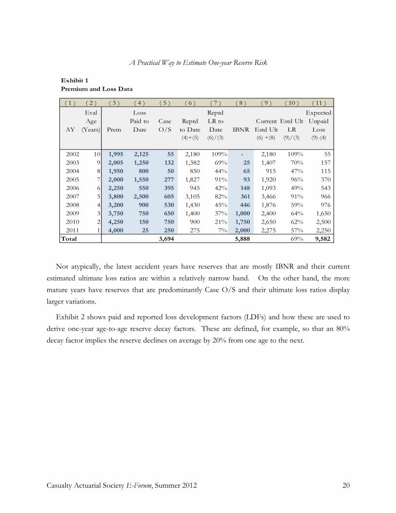
A Practical Way to Estimate One-year Reserve Risk
Casualty Actuarial Society E-Forum, Summer 2012 20
Not atypically, the latest accident years have reserves that are mostly IBNR and their current estimated ultimate loss ratios are within a relatively narrow band. On the other hand, the more mature years have reserves that are predominantly Case O/S and their ultimate loss ratios display larger variations.
Exhibit 2 shows paid and reported loss development factors (LDFs) and how these are used to derive one-year age-to-age reserve decay factors. These are defined, for example, so that an 80% decay factor implies the reserve declines on average by 20% from one age to the next.
Premium and Loss Data
( 1 ) ( 2 ) ( 3 ) ( 4 ) ( 5 ) ( 6 ) ( 7 ) ( 8 ) ( 9 ) ( 10 ) ( 11 )
AY
Eval Age
(Years) Prem
Loss Paid to Date
Case O/S
Reptd to Date
Reptd LR to Date IBNR
Current Estd Ult
Estd Ult LR
Expected Unpaid
Loss(4)+(5) (6)/(3) (6) +(8) (9)/(3) (9)-(4)
2002 10 1,995 2,125 55 2,180 109% - 2,180 109% 55 2003 9 2,005 1,250 132 1,382 69% 25 1,407 70% 157 2004 8 1,950 800 50 850 44% 65 915 47% 115 2005 7 2,000 1,550 277 1,827 91% 93 1,920 96% 370 2006 6 2,250 550 395 945 42% 148 1,093 49% 543 2007 5 3,800 2,500 605 3,105 82% 361 3,466 91% 966 2008 4 3,200 900 530 1,430 45% 446 1,876 59% 976 2009 3 3,750 750 650 1,400 37% 1,000 2,400 64% 1,650 2010 2 4,250 150 750 900 21% 1,750 2,650 62% 2,500 2011 1 4,000 25 250 275 7% 2,000 2,275 57% 2,250
Total 3,694 5,888 69% 9,582
Exhibit 1

A Practical Way to Estimate One-year Reserve Risk
Casualty Actuarial Society E-Forum, Summer 2012 21
Exhibit 3 shows the standard run-off triangles and the derivation of projected paid losses, Case O/S, and IBNR by calendar year. To explain the sequence of the calculation, we first use the Unpaid Decay factor for an accident year to figure out how much should be unpaid on average as of the next evaluation. This is shown in Exhibit 3-Table 1, while Exhibit 3-Table 2 shows the resulting estimates of paid loss by year.
Development Patterns to Decay Factors
( 1 ) ( 2 ) ( 3 ) ( 4 ) ( 5 ) ( 6 ) ( 7 ) ( 8 ) ( 9 ) ( 10 ) ( 11 )
Age
Reptd ATU LDF
Paid ATU LDF
Cumul Reptd
Cumul Paid
Increm Reptd
Increm Paid
Unreptd PCT
Unpaid PCT
IBNR -1 year Decay Factor
Unpaid - 1 yr
Decay Factor
1.0/(2) 1.0/(3) ∆(4) ∆(5) 1.0-(4) 1.0-(5) Col (8) Row ratios
Col (9) Row ratios
11 1.000 1.000 100.0% 100.0% 0.1% 1.0% 0.0% 0.0%10 1.001 1.010 99.9% 99.0% 0.4% 1.0% 0.1% 1.0% 0.000 0.0009 1.005 1.020 99.5% 98.0% 1.5% 2.8% 0.5% 2.0% 0.201 0.5058 1.020 1.050 98.0% 95.2% 1.9% 6.0% 2.0% 4.8% 0.254 0.4127 1.040 1.120 96.2% 89.3% 4.4% 9.3% 3.8% 10.7% 0.510 0.4446 1.090 1.250 91.7% 80.0% 4.8% 13.3% 8.3% 20.0% 0.466 0.5365 1.150 1.500 87.0% 66.7% 7.0% 33.3% 13.0% 33.3% 0.633 0.6004 1.250 3.000 80.0% 33.3% 13.3% 13.3% 20.0% 66.7% 0.652 0.5003 1.500 5.000 66.7% 20.0% 33.3% 10.0% 33.3% 80.0% 0.600 0.8332 3.000 10.000 33.3% 10.0% 16.7% 6.7% 66.7% 90.0% 0.500 0.8891 6.000 30.000 16.7% 3.3% 16.7% 3.3% 83.3% 96.7% 0.800 0.931
Exhibit 2

A Practical Way to Estimate One-year Reserve Risk
Casualty Actuarial Society E-Forum, Summer 2012 22
Next we project IBNR by applying the IBNR decay factors to current IBNR. The resulting projections for our example are shown in Exhibit3 -Table 3.
Projected Unpaid Loss Evaluation Lag
AYEval Age
Current Unpaid 1 2 3 4 5 6 7 8 9 10
2002 10 55 - - - - - - - - - - 2003 9 157 79 - - - - - - - - - 2004 8 115 47 24 - - - - - - - - 2005 7 370 164 68 34 - - - - - - - 2006 6 543 291 129 53 27 - - - - - - 2007 5 966 580 311 138 57 29 - - - - - 2008 4 976 488 293 157 70 29 14 - - - - 2009 3 1,650 1,375 688 413 221 98 40 20 - - - 2010 2 2,500 2,222 1,852 926 556 298 132 54 28 - - 2011 1 2,250 2,095 1,862 1,552 776 466 249 111 46 23 -
CY total 9,582 7,342 5,226 3,272 1,706 919 437 186 73 23 -
Exhibit 3 - Table 1
Projected Incremental Paid Loss Evaluation Lag
AYEval Age 1 2 3 4 5 6 7 8 9 10
2002 10 55 - - - - - - - - - 2003 9 78 79 - - - - - - - - 2004 8 68 23 24 - - - - - - - 2005 7 206 97 34 34 - - - - - - 2006 6 252 162 76 26 27 - - - - - 2007 5 386 269 173 81 28 29 - - - - 2008 4 488 195 136 87 41 14 14 - - - 2009 3 275 688 275 192 123 58 20 20 - - 2010 2 278 370 926 370 258 165 78 27 28 - 2011 1 155 233 310 776 310 216 139 65 23 23
CY total - 2,240 2,116 1,953 1,567 787 482 251 113 50 23
Exhibit 3 - Table 2
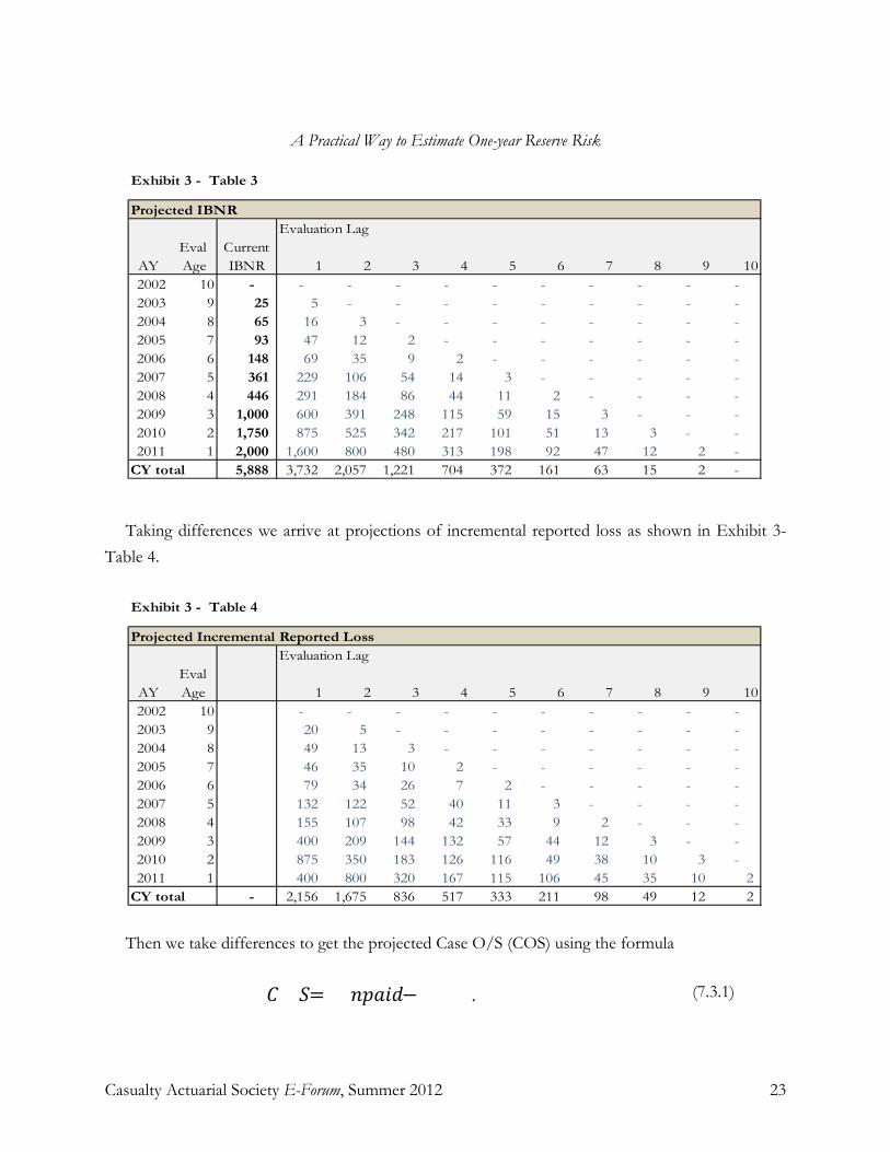
A Practical Way to Estimate One-year Reserve Risk
Casualty Actuarial Society E-Forum, Summer 2012 23
Taking differences we arrive at projections of incremental reported loss as shown in Exhibit 3-Table 4.
Then we take differences to get the projected Case O/S (COS) using the formula
𝐶𝐶𝐶𝐶𝑆𝑆= 𝑈𝑈𝑈𝑈𝑈𝑈𝑈𝑈𝑈𝑈𝑈𝑈−𝐼𝐼𝐵𝐵𝑁𝑁𝑅𝑅. (7.3.1)
Projected IBNREvaluation Lag
AYEval Age
Current IBNR 1 2 3 4 5 6 7 8 9 10
2002 10 - - - - - - - - - - - 2003 9 25 5 - - - - - - - - - 2004 8 65 16 3 - - - - - - - - 2005 7 93 47 12 2 - - - - - - - 2006 6 148 69 35 9 2 - - - - - - 2007 5 361 229 106 54 14 3 - - - - - 2008 4 446 291 184 86 44 11 2 - - - - 2009 3 1,000 600 391 248 115 59 15 3 - - - 2010 2 1,750 875 525 342 217 101 51 13 3 - - 2011 1 2,000 1,600 800 480 313 198 92 47 12 2 -
CY total 5,888 3,732 2,057 1,221 704 372 161 63 15 2 -
Exhibit 3 - Table 3
Projected Incremental Reported Loss Evaluation Lag
AYEval Age 1 2 3 4 5 6 7 8 9 10
2002 10 - - - - - - - - - - 2003 9 20 5 - - - - - - - - 2004 8 49 13 3 - - - - - - - 2005 7 46 35 10 2 - - - - - - 2006 6 79 34 26 7 2 - - - - - 2007 5 132 122 52 40 11 3 - - - - 2008 4 155 107 98 42 33 9 2 - - - 2009 3 400 209 144 132 57 44 12 3 - - 2010 2 875 350 183 126 116 49 38 10 3 - 2011 1 400 800 320 167 115 106 45 35 10 2
CY total - 2,156 1,675 836 517 333 211 98 49 12 2
Exhibit 3 - Table 4

A Practical Way to Estimate One-year Reserve Risk
Casualty Actuarial Society E-Forum, Summer 2012 24
Note Case O/S in some cases can reasonably be projected to increase the first few years during the run-off period. On the other hand, IBNR will typically decrease year by year.
7.4 Projecting Ultimate Risk by Year To decompose the ultimate risk into Case O/S and IBNR components, selections are made for
the ultimate CV and the κ parameter. Then with the initial Case O/S and IBNR balances, the respective CVs for Case O/S and IBNR may be derived as shown in Exhibit 4.
CV Coefficient Derivation
Item Value Source(1) CY 2011(2) Mean of Full Value of Ultimate Unpaid Loss 9,582 Ex 3 Tbl 1(3) Case O/S 3,694 Ex 3 Tbl 5(4) Mean IBNR 5,888 Ex 3 Tbl 3(5) CV of Ultimate Unpaid Loss 20.0% User selection(6) k = CV of IBNR versus CV of Case O/S 150.0% User selection(7) Stnd Dev of Ultimate Unpaid 1,916 (2)*(5)(8) Case OS CV Coefficient 0.200 sqrt{(7)2)/[(3)2+ ((6)*(4))2 ]}(9) IBNR CV Coefficient 0.300 (8)*(6)
Exhibit 4
Projected Case OS Loss Evaluation Lag
AYEval Age
Current Case OS 1 2 3 4 5 6 7 8 9 10
2002 10 55 - - - - - - - - - - 2003 9 132 74 - - - - - - - - - 2004 8 50 31 21 - - - - - - - - 2005 7 277 117 56 32 - - - - - - - 2006 6 395 222 94 44 25 - - - - - - 2007 5 605 351 204 84 43 26 - - - - - 2008 4 530 197 109 71 26 18 12 - - - - 2009 3 650 775 296 165 106 39 26 17 - - - 2010 2 750 1,347 1,327 584 339 197 81 41 25 - - 2011 1 250 495 1,062 1,072 463 267 157 64 34 21 -
CY total 3,694 3,609 3,168 2,051 1,001 547 276 123 59 21 -
Exhibit 3 - Table 5

A Practical Way to Estimate One-year Reserve Risk
Casualty Actuarial Society E-Forum, Summer 2012 25
Note that Equation 7.2.5 is used in Row 8 of Exhibit 4 and the selected κ is used to obtain Row 9.
Next, assume the respective CVs for Case O/S and IBNR are applicable for each year over the whole run-off period. Recall the Standard Formula uses a single CV for one-year reserve risk for each line of business and that this same CV applies for each year of the run-off period. The CVs under our method will evolve over the run-off period because the mix of Case O/S and IBNR will evolve. Because it reflects the changing mix of reserves, the proposed method should result in more accurate reserve risk estimates in any particular year than that produced using the single CV method of the Standard Formula.24
The calculation of the year-by-year variances is shown in Exhibit 5.
7.5 From Ultimate Risk to One-year Risk Next we derive one-year variance estimates by taking the difference between successive ultimate
variance projections. Figure 1 depicts the idea.
24 An even more sophisticated model could be developed in which the CVs of Case O/S and IBNR also evolve over time.
Projection of Year by Year Variance of Ultimate Unpaid
( 1 ) ( 2 ) ( 3 ) ( 4 ) ( 5 ) ( 6 ) ( 7 ) ( 8 ) ( 9 ) ( 10 )
CYEval Lag Case O/S IBNR
Total Unpaid
Stnd Dev from
Case O/S
Stnd Dev from
IBNR Variance Stnd Dev CV(3)+(4) (3)*CVCOS (4)*CVIBNR (6)2+(7)2 (8)1/2 (9)/(5)
2011 0 3,694 5,888 9,582 739 1,768 3,672,589 1,916 0.2002012 1 3,609 3,732 7,342 723 1,121 1,777,969 1,333 0.1822013 2 3,168 2,057 5,226 634 618 783,872 885 0.1692014 3 2,051 1,221 3,272 411 367 303,081 551 0.1682015 4 1,001 704 1,706 200 212 84,925 291 0.1712016 5 547 372 919 109 112 24,451 156 0.1702017 6 276 161 437 55 48 5,380 73 0.1682018 7 123 63 186 25 19 962 31 0.1672019 8 59 15 73 12 4 157 13 0.1712020 9 21 2 23 4 1 18 4 0.1822021 10 - - - - - - - 0.000
Exhibit 5

A Practical Way to Estimate One-year Reserve Risk
Casualty Actuarial Society E-Forum, Summer 2012 26
Figure 1
The differencing formula is based on three major assumptions:
• First, it presumes the estimates of mean unpaid loss subsequent to each evaluation do not change as the result of the intervening observations. This is behavior of unpaid loss estimates derived using the Bornheutter-Ferguson method, when LDFs and expected loss ratios (ELRs) are frozen.
• Second, it assumes the incremental paid losses from separate run-off years have no covariance with one another. This could likely be derived from the first assumption.
• Third, it assumes there is no change in the estimate of variance of paid loss for any year of run-off.
With these assumptions, differencing of the variances between ultimate unpaid for two consecutive year-end valuations produces the one-year variance during the year. A mathematical derivation is provided in Appendix B.
Reserve Risk
Year 1
Reserve Risk at Ultimate
End of Year 1
Reserve Risk
Year …
Reserve Risk
Year 2
Reserve Risk at Ultimate
Initial Estimate
Reserve Risk
Year …
Reserve Risk
Year 2
Reserve Risk
Year 1

A Practical Way to Estimate One-year Reserve Risk
Casualty Actuarial Society E-Forum, Summer 2012 27
One-year variance calculations for our example are shown in Exhibit 6. The first one-year variance is 1,894,620, which is the difference between the initial variance of 3,672,589 and the year-end variance of 1,777,969. With the variance and the mean, it is straightforward to derive the CV and other parameters of the associated one-year reserve risk lognormal as is done in columns (6) and (7) of Exhibit 6. In this table, the notation E[R] in column 5 stands for the expected total unpaid displayed in Exhibit 5. After the CV is calculated in column 5 of Exhibit 6, the lognormal parameters, µ and σ, are found separately for each year using the formulas shown in the calculation notes. Please see Appendix A for more detail. With the parameters, the 99.5th percentile may be readily computed and it is then straightforward to compute the amount excess of the mean as shown in column 10 of Exhibit 6. This is the standalone undiscounted SCR. It is useful to express the SCR as a percentage of the mean reserve as is done in column 11 of Exhibit 6. For any particular year, the calculations are similar to what would be done using the Standard Formula. The major
Projection of One -Year Variance and SCRs
( 1 ) ( 2 ) ( 3 ) ( 4 ) ( 5 ) ( 6 ) ( 7 ) ( 8 ) ( 9 ) ( 10 ) ( 11 )
CYUltimate Variance
One-Year Variance
One- Year Stnd Dev
One-Year CV σ µ Mean
Full Value
99.50th percentile
Full Value SCR
SCR as % of
reserve ∆(2) (3)1/2 (4)/E[R] (9) -(8) (10)/(8)
2011 3,672,589 1,894,620 1,376 0.144 0.14 9.16 9,582 13,706 4,124 43.0%2012 1,777,969 994,097 997 0.136 0.14 8.89 7,342 10,305 2,963 40.4%2013 783,872 480,790 693 0.133 0.13 8.55 5,226 7,280 2,054 39.3%2014 303,081 218,156 467 0.143 0.14 8.08 3,272 4,670 1,398 42.7%2015 84,925 60,473 246 0.144 0.14 7.43 1,706 2,443 737 43.2%2016 24,451 19,071 138 0.150 0.15 6.81 919 1,335 416 45.3%2017 5,380 4,419 66 0.152 0.15 6.07 437 637 201 46.0%2018 962 805 28 0.153 0.15 5.21 186 271 86 46.2%2019 157 139 12 0.161 0.16 4.28 73 109 36 49.1%
Percentage for SCR Percentile 99.5%Standard Normal Percentile 2.576
Calculation notes (6) σ = [ ln( 1+CV2)] 1/2
(7) µ = ln( E[R]) - 1/2 σ2
(8) Mean = E[R] = exp(µ + 1/2 σ2 ) (9) 99.5th percentile = exp(µ + 2.576 σ )
Exhibit 6

A Practical Way to Estimate One-year Reserve Risk
Casualty Actuarial Society E-Forum, Summer 2012 28
difference is that the Standard Formula SCR calculation uses the same CV for all years of run-off whereas the proposed approach has CVs that vary by year because the mix of Case O/S and IBNR changes by run-off year.
7.6 Discounted SCR and Technical Provision We compute the discounted mean unpaid loss for each year of run-off and then the associated
standalone SCR by applying the undiscounted SCR factor. This is similar to the approach taken in the Standard Formula where a fixed CV is used to get factors that are applied to discounted reserves. With the SCRs we compute the cost of capital amounts by year and discount those to get the standalone risk margin in the Technical Provision. Exhibit 7 shows these calculations.
Exhibit 8 shows the interest rates used in discounting. They are derived by summing the risk-free-rate and the illiquidity premium. While the rates were loosely taken from EIOPA charts, they are meant to be used here only for illustrative purposes. They should not be used in real applications. However, they do provide a rough idea of the magnitudes and shape of yield curve
Calculation of Discounted Reserve and Standalone Risk Margin
( 1 ) ( 2 ) ( 3 ) ( 4 ) ( 5 ) ( 6 ) ( 7 ) ( 8 )
CY Paid Loss
Full value Unpaid
Loss
Discounted Unpaid
LossSCR
Factor SCRCost of Capital
Discounted Cost of Capital
from Ex 3 Table 2
from Ex 3 Table 1
(3) *Ex 8 Col 5
from Ex 6 (5)*(4) CocRate*(6) (7) *Ex 8 Col 5
2011 - 9,582 9,056 43.0% 3,897 234 231 2012 2,240 7,342 7,020 40.4% 2,834 170 166 2013 2,116 5,226 5,042 39.3% 1,982 119 114 2014 1,953 3,272 3,175 42.7% 1,357 81 75 2015 1,567 1,706 1,659 43.2% 717 43 38 2016 787 919 897 45.3% 407 24 21 2017 482 437 428 46.0% 197 12 10 2018 251 186 182 46.2% 84 5 4 2019 113 73 72 49.1% 35 2 2 2020 50 23 23 56.6% 13 1 1 2021 23 - - 0.0% - - -
Total 9,582 7,613 457 429
6.00%Cost of Capital Rate
Exhibit 7

A Practical Way to Estimate One-year Reserve Risk
Casualty Actuarial Society E-Forum, Summer 2012 29
and the impact of the illiquidity premium.
Exhibit 9 shows the derivation of the final standalone Technical Provision for unpaid loss.25
Note that in this example that the effect of discounting more than offsets the explicit inclusion of a risk margin. In other examples, such as those for short tail lines, the risk margin often exceeds the magnitude of the discount. Stepping back, the overall impact is generally to arrive at a Technical 25 The impact of reinsurance has been omitted in this discussion.
Yield Curve, Illiquidity Premiums, and PV Factors
( 1 ) ( 2 ) ( 3 ) ( 4 ) ( 5 )
timeRisk-free
yieldIlliquidity Premium
Rate for Discounting PV Factor
yrs (2)+(3) (1.0+ (4))^-(1)
1 0.331% 0.710% 1.041% 0.9897 2 0.385% 0.710% 1.095% 0.9785 3 0.773% 0.710% 1.483% 0.9568 4 1.220% 0.710% 1.930% 0.9264 5 1.678% 0.710% 2.388% 0.8887 6 2.090% 0.710% 2.800% 0.8473 7 2.441% 0.710% 3.151% 0.8048 8 2.721% 0.710% 3.431% 0.7635 9 2.953% 0.710% 3.663% 0.7234 10 3.128% 0.710% 3.838% 0.6862 11 3.384% 0.710% 4.094% 0.6432
Exhibit 8
Derivation of Standalone Technical Provision for Unpaid Loss
Item Value Source(1) Mean of Full Value Ult Unpaid Loss 9,582 Ex 7 Col 3(2) Mean of Discounted Unpaid Loss 9,056 Ex 7 Col 4(3) Effect of Discount (526) (2) - (1)(4) Risk Margin 429 Ex 7 Col 8(5) Technical Provision 9,485 (1) + (3) + (4)
Exhibit 9

A Practical Way to Estimate One-year Reserve Risk
Casualty Actuarial Society E-Forum, Summer 2012 30
Provision not far off from the original mean of undiscounted unpaid losses. However, this result depends highly on the interest rate. Currently, interest rates are at historic lows. If they move up a few points, the Technical Provision for many long-tail lines could fall well below the undiscounted mean unpaid loss.
8. CONCLUSION
Our proposal is a very practical refinement of the Standard Formula. It is focused on finding one-year CVs that can be directly related to estimates of ultimate risk and to the types of reserves and how they evolve. In that sense it is a bridge between various known variables about which actuaries have some intuition and a new quantity, one-year reserve risk, about which actuaries know little. It provides a coherent framework within which recognition can be projected in a systematic and logical manner. Other methods do not use the information about risk contained in knowing the split between Case O/S and IBNR: this one does.
The method is also applicable in a wide range of circumstances as it employs user-selected patterns that need not be derived from data. For new businesses such data may not yet exist, but reserving actuaries may have selected paid patterns and reporting patterns to be used in reserving analysis. Another plus is that the method works well for long-tailed lines of business. Note that the proposed method is flexible, as it can be used at the level of business at which the enterprise is managed. There is no need to aggregate the data to make the algorithm work. In conclusion, this is a practical way to compute one-year reserve risk in an internal model. It is one of several methods to consider when deciding on how to quantify one-year reserve risk for Solvency II requirements.
APPENDIX A –LOGNORMAL STANDARD FORMULA CALCULATIONS
For a lognormal, X, with parameters (µ, σ), it is well known that
𝐵𝐵[𝑋𝑋] = 𝑒𝑒𝜇𝜇+12𝜎𝜎
2 𝑈𝑈𝑈𝑈𝑈𝑈 𝐵𝐵[𝑋𝑋2] = 𝑒𝑒2𝜇𝜇+2𝜎𝜎2 . (A.1)
Following the standard derivation we have
𝐶𝐶𝑃𝑃2 = 𝑒𝑒𝜎𝜎2 − 1. (A.2)
Thus we can derive:
𝜎𝜎= �ln(1 + 𝐶𝐶𝑃𝑃2). (A.3)
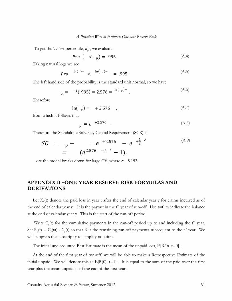
A Practical Way to Estimate One-year Reserve Risk
Casualty Actuarial Society E-Forum, Summer 2012 31
To get the 99.5% percentile, πp , we evaluate
𝑇𝑇𝑀𝑀𝑜𝑜𝑃𝑃�𝑋𝑋< 𝜋𝜋𝑈𝑈� = .995. (A.4)
Taking natural logs we see
𝑇𝑇𝑀𝑀𝑜𝑜𝑃𝑃�ln (𝑋𝑋)−𝜇𝜇σ
< ln�𝜋𝜋𝑈𝑈�−𝜇𝜇σ
�= .995. (A.5)
The left hand side of the probability is the standard unit normal, so we have
𝑧𝑧𝑈𝑈 = Φ−1(. 995) = 2.576 = ln�𝜋𝜋𝑈𝑈�−𝜇𝜇σ
. (A.6)
Therefore
ln�𝜋𝜋𝑈𝑈� = 𝜇𝜇+ 2.576 ∙𝜎𝜎, (A.7)
from which it follows that
𝜋𝜋𝑈𝑈 = 𝑒𝑒𝜇𝜇+2.576∙𝜎𝜎. (A.8)
Therefore the Standalone Solvency Capital Requirement (SCR) is
𝑆𝑆𝐶𝐶𝑅𝑅= 𝜋𝜋𝑈𝑈 −𝐵𝐵[𝑋𝑋] = 𝑒𝑒𝜇𝜇+2.576∙𝜎𝜎− 𝑒𝑒𝜇𝜇+12𝜎𝜎
2 = 𝐵𝐵[𝑋𝑋](𝑒𝑒2.576∙𝜎𝜎−.5𝜎𝜎2 − 1).
(A.9)
Note the model breaks down for large CV, where σ >5.152.
APPENDIX B –ONE-YEAR RESERVE RISK FORMULAS AND DERIVATIONS
Let Xy(t) denote the paid loss in year t after the end of calendar year y for claims incurred as of the end of calendar year y. It is the payout in the tth year of run-off. Use t=0 to indicate the balance at the end of calendar year y. This is the start of the run-off period.
Write Cy(t) for the cumulative payments in the run-off period up to and including the tth year. Set Ry(t) = Cy(ω) - Cy(t) so that R is the remaining run-off payments subsequent to the tth year. We will suppress the subscript y to simplify notation.
The initial undiscounted Best Estimate is the mean of the unpaid loss, E[R(0)|t=0] .
At the end of the first year of run-off, we will be able to make a Retrospective Estimate of the initial unpaid. We will denote this as E[R(0)|t=1]. It is equal to the sum of the paid over the first year plus the mean unpaid as of the end of the first year:

A Practical Way to Estimate One-year Reserve Risk
Casualty Actuarial Society E-Forum, Summer 2012 32
𝐵𝐵[𝑅𝑅(0)|𝑡𝑡 = 1] = 𝑋𝑋(1) + 𝐵𝐵[𝑅𝑅(1)|𝑡𝑡 = 1] (B.1)
The one-year variance is equal to:
𝐶𝐶𝑈𝑈𝑒𝑒−𝑦𝑦𝑒𝑒𝑈𝑈𝑀𝑀 𝑃𝑃𝑈𝑈𝑀𝑀𝑈𝑈𝑈𝑈𝑈𝑈𝑉𝑉𝑒𝑒= 𝐵𝐵 [ (𝐵𝐵[𝑅𝑅(0)|𝑡𝑡 = 1] − 𝐵𝐵[𝑅𝑅(0)|𝑡𝑡 = 0])2 ] (B.2)
Under the Bornheutter-Ferguson (BF) method, the expected value at a given evaluation data of unpaid loss beyond a given subsequent date is independent of the evaluation date. In particular:
𝐵𝐵[𝑅𝑅(1)|𝑡𝑡 = 1] = 𝐵𝐵[𝑅𝑅(1)|𝑡𝑡 = 0] (B.3)
This implies:
𝐶𝐶𝑈𝑈𝑒𝑒 𝑌𝑌𝑒𝑒𝑈𝑈𝑀𝑀 𝑃𝑃𝑈𝑈𝑀𝑀𝑈𝑈𝑈𝑈𝑈𝑈𝑉𝑉𝑒𝑒= 𝐵𝐵 [ (𝑋𝑋(1) − 𝐵𝐵[𝑋𝑋(1)|𝑡𝑡 = 0])2 ] = 𝑃𝑃𝑈𝑈𝑀𝑀(𝑋𝑋(1))
(B.4)
Now consider the ultimate variance of the initial unpaid run-off is:
𝑃𝑃𝑈𝑈𝑀𝑀(𝑅𝑅(0)| 𝑡𝑡 = 0) =
� 𝑃𝑃𝑈𝑈𝑀𝑀(𝑋𝑋(𝐿𝐿)|𝑡𝑡 = 0) + � 𝐶𝐶𝑜𝑜𝑣𝑣(𝑋𝑋(𝑀𝑀),𝑋𝑋(𝐿𝐿)|𝑡𝑡 = 0)𝑀𝑀≠𝐿𝐿
𝜔𝜔
𝐿𝐿=1
(B.5)
Similarly, the ultimate variance of the unpaid run-off at the end of year one is:
𝑃𝑃𝑈𝑈𝑀𝑀(𝑅𝑅(1)| 𝑡𝑡 = 1) =
� 𝑃𝑃𝑈𝑈𝑀𝑀(𝑋𝑋(𝐿𝐿)|𝑡𝑡 = 1) + � 𝐶𝐶𝑜𝑜𝑣𝑣(𝑋𝑋(𝑀𝑀),𝑋𝑋(𝐿𝐿)|𝑡𝑡 = 1)𝑀𝑀≠𝐿𝐿,𝑀𝑀>1,𝐿𝐿>1
𝜔𝜔
𝐿𝐿=2
(B.6)
Now assume all the covariances in B.5 and B.6 are zero. This is a generalization of the
Bornheutter-Ferguson assumption. Subtracting B.6 from B.5 and using this vanishing covariance assumption, we obtain:

A Practical Way to Estimate One-year Reserve Risk
Casualty Actuarial Society E-Forum, Summer 2012 33
𝑃𝑃𝑈𝑈𝑀𝑀(𝑅𝑅(0)| 𝑡𝑡 = 0) −𝑃𝑃𝑈𝑈𝑀𝑀(𝑅𝑅(1)| 𝑡𝑡 = 1) =
� 𝑃𝑃𝑈𝑈𝑀𝑀(𝑋𝑋(𝐿𝐿)|𝑡𝑡 = 0) −𝜔𝜔
𝐿𝐿=1 � 𝑃𝑃𝑈𝑈𝑀𝑀(𝑋𝑋(𝐿𝐿)|𝑡𝑡 = 1)
𝜔𝜔
𝐿𝐿=2
(B.7)
Finally, we suppose that the variances of the incremental unpaid amounts do not change from one evaluation to the next. Under these admittedly stringent assumptions we have:
𝑃𝑃𝑈𝑈𝑀𝑀(𝑅𝑅(0)| 𝑡𝑡 = 0) −𝑃𝑃𝑈𝑈𝑀𝑀(𝑅𝑅(1)| 𝑡𝑡 = 1) = 𝑃𝑃𝑈𝑈𝑀𝑀(𝑋𝑋(1)).
(B.8)
Comparing B.8 to B.4 leads to the result shown in Figure 1.
Acknowledgment
The author gratefully acknowledges the support of Joshua London who read drafts and provided insightful comments. Disclaimers
This paper is solely the work of the author and the opinions expressed herein are solely those of the author. This paper contains no express or implied presentation or endorsement of the views of the author’s prior employers. No liability whatsoever is assumed for any losses, direct or indirect, that may result from use of the methods described in this paper.

A Practical Way to Estimate One-year Reserve Risk
Casualty Actuarial Society E-Forum, Summer 2012 34
REFERENCES
[1] Actuarial Standards Board, ASOP #43, 2007. [2] Boor, Joseph, “A Macroeconomic View of the Insurance Marketplace,” CAS Exam 5 Study Kit, 2000. [3] Boumezoued, Alexandre, Yoguba Angoua, Devineau, Laurent and Boisseau Jean-Philippe, “One-year reserve risk
including a tail factor: closed formula and bootstrap approaches,” Working paper submitted to ASTIN, 2011. [4] CEIOPS, “QIS5 Technical Specifications,” July 2010. [5] EIOPA Joint Working Group (JWG), “Calibration of the Premium and Reserve Risk Factors in the Standard
Formula in Solvency II,” December 2011. [6] England, Peter, “Reserving risk, risk margins, and solvency: Re-tuning your mind,” EMB Solvency II Briefing, January
2010. [7] LLOYDS, “Solvency II Core Validation Workshop,” May 2011. [8] Merz, Michael and Wuthrich, Mario V, “Modeling the Claims Development Result for Solvency Purposes,”
Casualty Actuarial Society E-Forum, Fall 2008, p. 542-568. [9] Miccolis, Robert S and Heppen, David E, “A Practical Approach to Risk Margins in the Measurement of
Insurance Liabilities for Property and Casualty (General Insurance) under Developing International Financial Reporting Standards,” 2010.
[10] Ohlsson, Esbjorn and Lauzeningks, Jan, “ The one-year non-life insurance risk,” ASTIN Colloquium 2008. [11] Rehmann, Zia and Klugman, Stuart, “Quantifying Uncertainty In Reserve Estimates,” Variance 2010, Vol. 04,
Issue 01, p. 30-46. [12] Schmidt, Neal, “ Discount Rate for Reserves Should Not be Increased for Illiquidity,” Actuarial Review, February
2011, Vol. 38, No.1, p. 26. [13] Taleb, Nassim, The Black Swan” Second Edition, 2010, Random House. [14] Underwood, Alice and Zhu, J. , “A Top-Down Approach to Understanding Uncertainty in Loss Ratio
Estimation,” Variance 2009, Vol. 3, Issue 01, p. 31-41. [15] Wacek, M., “The Path of the Ultimate Loss Ratio Estimate”, Casualty Actuarial Society Forum, Winter, 2007 p. 339-
370. [16] White, Stuart and Margetts, Simon, “A link between the one–year and ultimate perspective on insurance risk,”
GIRO conference, October 2010. Abbreviations and notations Collect here in alphabetical order all abbreviations and notations used in the paper BE, Best Estimate RM, Risk Margin BF, Bornheutter-Ferguson SCR, Solvency Capital Requirement COC, Cost-of-Capital SF, Standard Formula DFCL, Distribution Free Chain Ladder TP, Technical Provision IBNR, Incurred But Not Reported Biography of the Author
Ira Robbin has held positions with Endurance, Partner Re, CIGNA PC, and INA working in several corporate and pricing actuarial roles. Ira has an undergraduate degree in Math from Michigan State and PhD in Math from Rutgers University. He has written papers on risk load, development patterns, IBNR formulas, ROE, Coherent Capital and other topics.

Standalone One‐year Reserve Risk Calculation
Company Currency
Business Unit/LOB Units
Evaluation at end of year
Reserves and Development Patterns Yield Rates
( 1 ) ( 2 ) ( 3 ) ( 4 ) ( 5 ) ( 6 ) ( 7 ) ( 8 ) ( 9 ) ( 1 ) ( 2 ) ( 3 )
AY
Eval Age (Years) Prem
Loss Paid to Date
Case O/S IBNR
Expected Unpaid Loss
Reptd ATU LDF
Paid
ATU LDF Duration
Risk‐free yield
Illiquidity Premium
(5)+(6) yrs
2002 10 1,995 2,125 55 ‐ 55 1.001 1.010 1 0.331% 0.710%
2003 9 2,005 1,250 132 25 157 1.005 1.020 2 0.385% 0.710%
2004 8 1,950 800 50 65 115 1.020 1.050 3 0.773% 0.710%
2005 7 2,000 1,550 277 93 370 1.040 1.120 4 1.220% 0.710%
2006 6 2,250 550 395 148 543 1.090 1.250 5 1.678% 0.710%
2007 5 3,800 2,500 605 361 966 1.150 1.500 6 2.090% 0.710%
2008 4 3,200 900 530 446 976 1.250 3.000 7 2.441% 0.710%
2009 3 3,750 750 650 1,000 1,650 1.500 5.000 8 2.721% 0.710%
2010 2 4,250 150 750 1,750 2,500 3.000 10.000 9 2.953% 0.710%
2011 1 4,000 25 250 2,000 2,250 6.000 30.000 10 3.128% 0.710%
Total 3,694 5,888 9,582 11 3.384% 0.710%
Risk Parameters Color codes
(1) CV of Ultimate Unpaid Loss 20.0%
(2) k = CV of IBNR versus CV of Case O/S 150.0%
(3) Cost‐of‐capital rate 6.0%
Name/alpha data
Numeric data/user selections
Numeric data from regulator
000
Input Sheet ‐ A Practical Way to Estimate One‐year Reserve Risk
USDPC Company
ABC Casualty Unit
2011
Page 1

Standalone One‐year Reserve Risk Calculation
PC Company
ABC Casualty Unit
Premium and Loss Data
( 1 ) ( 2 ) ( 3 ) ( 4 ) ( 5 ) ( 6 ) ( 7 ) ( 8 ) ( 9 ) ( 10 ) ( 11 )
AY
Eval Age
(Years) Prem
Loss Paid to Date
Case O/S
Reptd to Date
Reptd LR to Date IBNR
Current Estd Ult
Estd Ult LR
Expected Unpaid Loss
(4)+(5) (6)/(3) (6) +(8) (9)/(3) (5)+(8)
2002 10 1,995 2,125 55 2,180 109% ‐ 2,180 109% 55 2003 9 2,005 1,250 132 1,382 69% 25 1,407 70% 157 2004 8 1,950 800 50 850 44% 65 915 47% 115 2005 7 2,000 1,550 277 1,827 91% 93 1,920 96% 370 2006 6 2,250 550 395 945 42% 148 1,093 49% 543 2007 5 3,800 2,500 605 3,105 82% 361 3,466 91% 966 2008 4 3,200 900 530 1,430 45% 446 1,876 59% 976 2009 3 3,750 750 650 1,400 37% 1,000 2,400 64% 1,650 2010 2 4,250 150 750 900 21% 1,750 2,650 62% 2,500 2011 1 4,000 25 250 275 7% 2,000 2,275 57% 2,250
Total 3,694 5,888 69% 9,582
Exhibit 1
Page 2

Standalone One‐year Reserve Risk Calculation
PC Company
ABC Casualty Unit
Development Patterns to Decay Factors
( 1 ) ( 2 ) ( 3 ) ( 4 ) ( 5 ) ( 6 ) ( 7 ) ( 8 ) ( 9 ) ( 10 ) ( 11 )
Age
Reptd ATU LDF
Paid
ATU LDF
Cumul Reptd
Cumul Paid
Increm Reptd
Increm Paid
Unreptd PCT
Unpaid
PCT
IBNR
‐1 year Decay Factor
Unpaid ‐1 yr
Decay Factor
1.0/(2) 1.0/(3) ∆(4) ∆(5) 1.0‐(4) 1.0‐(5) Col (8) Row ratios
Col (9) Row ratios
10 1.001 1.010 99.9% 99.0% 0.4% 1.0% 0.1% 1.0% 0.000 0.000
9 1.005 1.020 99.5% 98.0% 1.5% 2.8% 0.5% 2.0% 0.201 0.505
8 1.020 1.050 98.0% 95.2% 1.9% 6.0% 2.0% 4.8% 0.254 0.412
7 1.040 1.120 96.2% 89.3% 4.4% 9.3% 3.8% 10.7% 0.510 0.444
6 1.090 1.250 91.7% 80.0% 4.8% 13.3% 8.3% 20.0% 0.466 0.536
5 1.150 1.500 87.0% 66.7% 7.0% 33.3% 13.0% 33.3% 0.633 0.600
4 1.250 3.000 80.0% 33.3% 13.3% 13.3% 20.0% 66.7% 0.652 0.500
3 1.500 5.000 66.7% 20.0% 33.3% 10.0% 33.3% 80.0% 0.600 0.833
2 3.000 10.000 33.3% 10.0% 16.7% 6.7% 66.7% 90.0% 0.500 0.889
1 6.000 30.000 16.7% 3.3% 16.7% 3.3% 83.3% 96.7% 0.800 0.931
Exhibit 2
Page 3

Standalone One‐year Reserve Risk Calculation
Projection Triangles
PC Company
ABC Casualty Unit
Projected Unpaid Loss
Evaluation Lag
AY
Eval Age
Current Unpaid 1 2 3 4 5 6 7 8 9 10
2002 10 55 ‐ ‐ ‐ ‐ ‐ ‐ ‐ ‐ ‐ ‐ 2003 9 157 79 ‐ ‐ ‐ ‐ ‐ ‐ ‐ ‐ ‐ 2004 8 115 47 24 ‐ ‐ ‐ ‐ ‐ ‐ ‐ ‐ 2005 7 370 164 68 34 ‐ ‐ ‐ ‐ ‐ ‐ ‐ 2006 6 543 291 129 53 27 ‐ ‐ ‐ ‐ ‐ ‐ 2007 5 966 580 311 138 57 29 ‐ ‐ ‐ ‐ ‐ 2008 4 976 488 293 157 70 29 14 ‐ ‐ ‐ ‐ 2009 3 1,650 1,375 688 413 221 98 40 20 ‐ ‐ ‐ 2010 2 2,500 2,222 1,852 926 556 298 132 54 28 ‐ ‐ 2011 1 2,250 2,095 1,862 1,552 776 466 249 111 46 23 ‐ CY total 9,582 7,342 5,226 3,272 1,706 919 437 186 73 23 ‐
Projected Incremental Paid Loss
Evaluation Lag
AY
Eval Age 1 2 3 4 5 6 7 8 9 10
2002 10 55 ‐ ‐ ‐ ‐ ‐ ‐ ‐ ‐ ‐ 2003 9 78 79 ‐ ‐ ‐ ‐ ‐ ‐ ‐ ‐ 2004 8 68 23 24 ‐ ‐ ‐ ‐ ‐ ‐ ‐ 2005 7 206 97 34 34 ‐ ‐ ‐ ‐ ‐ ‐ 2006 6 252 162 76 26 27 ‐ ‐ ‐ ‐ ‐ 2007 5 386 269 173 81 28 29 ‐ ‐ ‐ ‐ 2008 4 488 195 136 87 41 14 14 ‐ ‐ ‐ 2009 3 275 688 275 192 123 58 20 20 ‐ ‐ 2010 2 278 370 926 370 258 165 78 27 28 ‐ 2011 1 155 233 310 776 310 216 139 65 23 23 CY total ‐ 2,240 2,116 1,953 1,567 787 482 251 113 50 23
Exhibit 3 ‐ Table 1
Exhibit 3 ‐ Table 2
Page 4

Standalone One‐year Reserve Risk Calculation
Projection Triangles
PC Company
ABC Casualty Unit
Projected IBNR
Evaluation Lag
AY
Eval
AgeCurrent IBNR 1 2 3 4 5 6 7 8 9 10
2002 10 ‐ ‐ ‐ ‐ ‐ ‐ ‐ ‐ ‐ ‐ ‐ 2003 9 25 5 ‐ ‐ ‐ ‐ ‐ ‐ ‐ ‐ ‐ 2004 8 65 16 3 ‐ ‐ ‐ ‐ ‐ ‐ ‐ ‐ 2005 7 93 47 12 2 ‐ ‐ ‐ ‐ ‐ ‐ ‐ 2006 6 148 69 35 9 2 ‐ ‐ ‐ ‐ ‐ ‐ 2007 5 361 229 106 54 14 3 ‐ ‐ ‐ ‐ ‐ 2008 4 446 291 184 86 44 11 2 ‐ ‐ ‐ ‐ 2009 3 1,000 600 391 248 115 59 15 3 ‐ ‐ ‐ 2010 2 1,750 875 525 342 217 101 51 13 3 ‐ ‐ 2011 1 2,000 1,600 800 480 313 198 92 47 12 2 ‐ CY total 5,888 3,732 2,057 1,221 704 372 161 63 15 2 ‐
Projected Incremental Reported Loss
Evaluation Lag
AY
Eval Age 1 2 3 4 5 6 7 8 9 10
2002 10 ‐ ‐ ‐ ‐ ‐ ‐ ‐ ‐ ‐ ‐ 2003 9 20 5 ‐ ‐ ‐ ‐ ‐ ‐ ‐ ‐ 2004 8 49 13 3 ‐ ‐ ‐ ‐ ‐ ‐ ‐ 2005 7 46 35 10 2 ‐ ‐ ‐ ‐ ‐ ‐ 2006 6 79 34 26 7 2 ‐ ‐ ‐ ‐ ‐ 2007 5 132 122 52 40 11 3 ‐ ‐ ‐ ‐ 2008 4 155 107 98 42 33 9 2 ‐ ‐ ‐ 2009 3 400 209 144 132 57 44 12 3 ‐ ‐ 2010 2 875 350 183 126 116 49 38 10 3 ‐ 2011 1 400 800 320 167 115 106 45 35 10 2 CY total ‐ 2,156 1,675 836 517 333 211 98 49 12 2
Exhibit 3 ‐ Table 3
Exhibit 3 ‐ Table 4
Page 5

Standalone One‐year Reserve Risk Calculation
Projection Triangles
PC Company
ABC Casualty Unit
Projected Case OS Loss
Evaluation Lag
AY
Eval Age
Current Case OS 1 2 3 4 5 6 7 8 9 10
2002 10 55 ‐ ‐ ‐ ‐ ‐ ‐ ‐ ‐ ‐ ‐ 2003 9 132 74 ‐ ‐ ‐ ‐ ‐ ‐ ‐ ‐ ‐ 2004 8 50 31 21 ‐ ‐ ‐ ‐ ‐ ‐ ‐ ‐ 2005 7 277 117 56 32 ‐ ‐ ‐ ‐ ‐ ‐ ‐ 2006 6 395 222 94 44 25 ‐ ‐ ‐ ‐ ‐ ‐ 2007 5 605 351 204 84 43 26 ‐ ‐ ‐ ‐ ‐ 2008 4 530 197 109 71 26 18 12 ‐ ‐ ‐ ‐ 2009 3 650 775 296 165 106 39 26 17 ‐ ‐ ‐ 2010 2 750 1,347 1,327 584 339 197 81 41 25 ‐ ‐ 2011 1 250 495 1,062 1,072 463 267 157 64 34 21 ‐ CY total 3,694 3,609 3,168 2,051 1,001 547 276 123 59 21 ‐
Exhibit 3 ‐ Table 5
Page 6

Standalone One‐Year Reserve Risk Calculation
PC Company
ABC Casualty Unit
CV Coefficient Derivation
Item Value Source
(1) CY Year End 2011
(2) Mean of Full Value of Ultimate Unpaid Loss 9,582 Ex 3 Tbl 1(3) Case O/S 3,694 Ex 3 Tbl 5(4) Mean IBNR 5,888 Ex 3 Tbl 3(5) CV of Ultimate Unpaid Loss 20.0% User selection(6) k = CV of IBNR versus CV of Case O/S 150.0% User selection(7) Stnd Dev of Ultimate Unpaid 1,916 (2)*(5)
(8) Case OS CV Coefficient 0.200 (7)2)/[(3)2+ ((6)*(4))2 ]
(9) IBNR CV Coefficient 0.300 (8)*(6)
Exhibit 4
Page 7
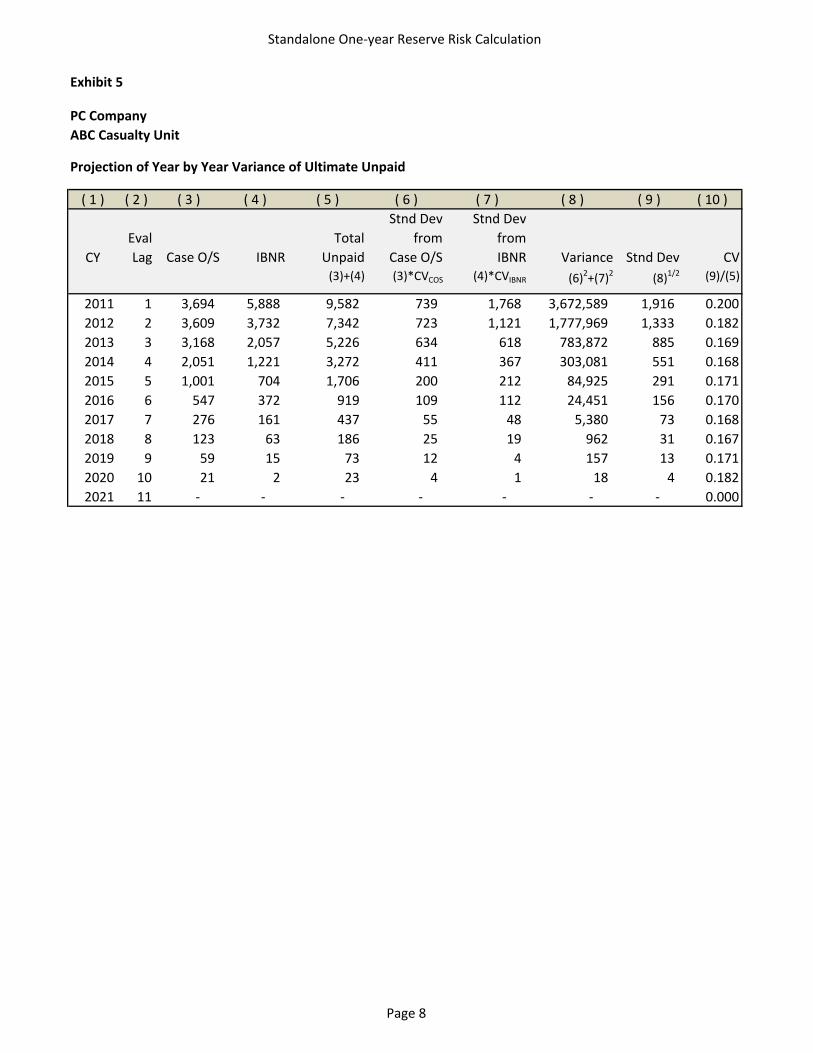
Standalone One‐year Reserve Risk Calculation
PC Company
ABC Casualty Unit
Projection of Year by Year Variance of Ultimate Unpaid
( 1 ) ( 2 ) ( 3 ) ( 4 ) ( 5 ) ( 6 ) ( 7 ) ( 8 ) ( 9 ) ( 10 )
CY
Eval Lag Case O/S IBNR
Total Unpaid
Stnd Dev from
Case O/S
Stnd Dev from
IBNR Variance Stnd Dev CV(3)+(4) (3)*CVCOS (4)*CVIBNR (6)2+(7)2 (8)1/2 (9)/(5)
2011 1 3,694 5,888 9,582 739 1,768 3,672,589 1,916 0.200
2012 2 3,609 3,732 7,342 723 1,121 1,777,969 1,333 0.182
2013 3 3,168 2,057 5,226 634 618 783,872 885 0.169
2014 4 2,051 1,221 3,272 411 367 303,081 551 0.168
2015 5 1,001 704 1,706 200 212 84,925 291 0.171
2016 6 547 372 919 109 112 24,451 156 0.170
2017 7 276 161 437 55 48 5,380 73 0.168
2018 8 123 63 186 25 19 962 31 0.167
2019 9 59 15 73 12 4 157 13 0.171
2020 10 21 2 23 4 1 18 4 0.182
2021 11 ‐ ‐ ‐ ‐ ‐ ‐ ‐ 0.000
Exhibit 5
Page 8

Standalone One‐year Reserve Risk Calculation
PC Company
ABC Casualty Unit
Projection of One ‐Year Variance and SCRs
( 1 ) ( 2 ) ( 3 ) ( 4 ) ( 5 ) ( 6 ) ( 7 ) ( 8 ) ( 9 ) ( 10 ) ( 11 )
CY
Ultimate Variance
One‐Year Variance
One‐ Year Stnd Dev
One‐Year CV Mean
Full Value 99.50th p'ctile
Full Value SCR
SCR as % of
reserve ∆(2) (3)1/2 (4)/E[R] (9) ‐(8) (10)/(8)
2011 3,672,589 1,894,620 1,376 0.144 0.14 9.16 9,582 13,706 4,124 43.0%
2012 1,777,969 994,097 997 0.136 0.14 8.89 7,342 10,305 2,963 40.4%
2013 783,872 480,790 693 0.133 0.13 8.55 5,226 7,280 2,054 39.3%
2014 303,081 218,156 467 0.143 0.14 8.08 3,272 4,670 1,398 42.7%
2015 84,925 60,473 246 0.144 0.14 7.43 1,706 2,443 737 43.2%
2016 24,451 19,071 138 0.150 0.15 6.81 919 1,335 416 45.3%
2017 5,380 4,419 66 0.152 0.15 6.07 437 637 201 46.0%
2018 962 805 28 0.153 0.15 5.21 186 271 86 46.2%
2019 157 139 12 0.161 0.16 4.28 73 109 36 49.1%
Percentage for SCR Percentile 99.5%
Standard Normal Percentile 2.576
Calculation notes (6) = [ ln( 1+CV2)] 1/2
(7) = ln( E[R]) ‐ 1/2 2
(8) Mean = E[R] = exp(2 ) (9) 99.5th percentile = exp()
Exhibit 6
Page 9

Standalone One‐year Reserve Risk Calculation
PC Company
ABC Casualty Unit
Calculation of Discounted Reserve and Standalone Risk Margin
( 1 ) ( 2 ) ( 3 ) ( 4 ) ( 5 ) ( 6 ) ( 7 ) ( 8 )
CY Paid LossFull value
Unpaid LossDiscounted
Unpaid LossSCR
Factor SCR
Cost of Capital
Discounted Cost of Capital
from Ex 3 Table 2
from Ex 3 Table 1
(3) *Ex 8 Col 5
from Ex 6 (5)*(4) CocRate*(6) (7) *Ex 8 Col 5
2011 ‐ 9,582 9,056 43.0% 3,897 234 231 2012 2,240 7,342 7,020 40.4% 2,834 170 166 2013 2,116 5,226 5,042 39.3% 1,982 119 114 2014 1,953 3,272 3,175 42.7% 1,357 81 75 2015 1,567 1,706 1,659 43.2% 717 43 38 2016 787 919 897 45.3% 407 24 21 2017 482 437 428 46.0% 197 12 10 2018 251 186 182 46.2% 84 5 4 2019 113 73 72 49.1% 35 2 2 2020 50 23 23 56.6% 13 1 1 2021 23 ‐ ‐ 0.0% ‐ ‐ ‐
Total 9,582 7,613 457 429
6.00%Cost of Capital Rate
Exhibit 7
Page 10

Standalone One‐year Reserve Risk Calculation
PC Company
ABC Casualty Unit
Yield Curve, Illiquidity Premiums, and PV Factors
( 1 ) ( 2 ) ( 3 ) ( 4 ) ( 5 )
time
Risk‐free yield
Illiquidity Premium
Rate for Discounting PV Factor
yrs (2)+(3) (1.0+ (4))^‐(1)
1 0.331% 0.710% 1.041% 0.9897 2 0.385% 0.710% 1.095% 0.9785 3 0.773% 0.710% 1.483% 0.9568 4 1.220% 0.710% 1.930% 0.9264 5 1.678% 0.710% 2.388% 0.8887 6 2.090% 0.710% 2.800% 0.8473 7 2.441% 0.710% 3.151% 0.8048 8 2.721% 0.710% 3.431% 0.7635 9 2.953% 0.710% 3.663% 0.7234 10 3.128% 0.710% 3.838% 0.6862 11 3.384% 0.710% 4.094% 0.6432
Exhibit 8
Page 11

Standalone One‐year Reserve Risk Calculation
PC Company
ABC Casualty Unit
Derivation of Standalone Technical Provision for Unpaid Loss
Item Value Source
(1) Mean of Full Value Ult Unpaid Loss 9,582 Ex 7 Col 3(2) Mean of Discounted Unpaid Loss 9,056 Ex 7 Col 4(3) Effect of Discount (526) (2) ‐ (1)(4) Risk Margin 429 Ex 7 Col 8(5) Technical Provision 9,485 (1) + (3) + (4)
Exhibit 9
Page 12

Proposal 2012 Reserves Call Paper Program 1
© Copyright 2012 National Council on Compensation Insurance, Inc. All Rights Reserved.
A Total Credibility Approach to Pool Reserving
Frank Schmid
______________________________________________________________________________ Abstract Motivation. Among other services in the assigned risk market, NCCI provides actuarial services for the National Workers Compensation Reinsurance Pooling Mechanism (NWCRP), the Massachusetts Workers’ Compensation Assigned Risk Pool, the Michigan Workers’ Compensation Placement Facility, and the New Mexico Workers’ Compensation Assigned Risk Pool. Pool reserving triangles pose specific challenges as they may be sparsely populated; this is because states may have left the NWCRP, recently joined it, or re-joined it after several years of absence. Furthermore, triangles of partial coverage states may have unpopulated cells due to not having experienced a claim in a given policy year. Method. There are two credibility aspects to Pool reserving to be addressed. First, the degree of variability of the link ratios may differ across states, possibly (but not necessarily entirely) due to differences in size of the assigned risk market across states. Second, the number of link ratios available varies greatly across states, from fully populated diagonals to very few observations per diagonal or, for some partial coverage states, to no observations at all. To address these challenges, a comprehensive credibility approach has been developed, where the credibility-adjustment applies to the data-generating process as opposed to the outcome. This new concept, called Total Credibility, rests on multilevel (hierarchical) modeling, which implies that the Pool triangles of all states are estimated simultaneously. Results. The model is applied to the logarithmic paid plus case link ratios of the latest five diagonals of the Pool triangles of 45 jurisdictions, some of which are partial coverage states. Diagnostic charts of in-sample fit show that the model is well suited for replicating the observed data. Further, diagnostic charts of forecast errors indicate that the structure of the model is a proper representation of the data-generating process. Availability. The model was implemented in R (http://cran.r-project.org/) using the sampling platform JAGS (Just Another Gibbs Sampler, http://www-ice.iarc.fr/~martyn/software/jags/). JAGS was linked to R by means of the R package rjags (http://cran.r-project.org/web/packages/rjags/index.html). Keywords. Pool Reserving, Growth Curve, Total Credibility
______________________________________________________________________________
1. INTRODUCTION
Among other services in the assigned risk market, NCCI provides actuarial services for the
National Workers Compensation Reinsurance Pooling Mechanism (NWCRP), the Massachusetts
Workers’ Compensation Assigned Risk Pool, the Michigan Workers’ Compensation Placement
Facility, and the New Mexico Workers’ Compensation Assigned Risk Pool. Pool reserving triangles
pose specific challenges as they may be sparsely populated; this is because states may have left the
NWCRP, recently joined it, or re-joined it after several years of absence. Furthermore, triangles of
partial coverage states may have unpopulated cells due to not having experienced a claim in a given
policy year.
There are two credibility aspects to Pool reserving to be addressed. First, the degree of variability
of the link ratios may differ across states, possibly (but not necessarily entirely) due to differences in

A Total Credibility Approach to Pool Reserving
Proposal 2012 Reserves Call Paper Program 2
© Copyright 2012 National Council on Compensation Insurance, Inc. All Rights Reserved.
size of the assigned risk market. Second, the number of link ratios available varies greatly across
states, from fully populated diagonals to very few observations per diagonal or, for some partial
coverage states, to no observations at all. To address these challenges, a comprehensive credibility
approach has been developed, where the credibility-adjustment applies to the data-generating
process, as opposed to its outcome. This new concept, called Total Credibility, rests on multilevel
(hierarchical) modeling. The parameters of the data-generating process of all states are estimated
simultaneously, with each state-level parameter being drawn from a parent distribution. This way, all
state-level parameters incorporate information from all states.
1.1 Research Context
Gelman and Hill [3] offer a textbook introduction to multilevel (hierarchical) modeling. In
multilevel modeling, credibility is implemented by means of partial pooling (or, synonymously,
shrinkage). The concept of partial pooling is akin to (and, in specific instances equivalent to)
Bühlmann credibility.
Let be one of the parameters that govern the data-generating process. In partial pooling, the
parameter is allowed to vary across the units of observations; in NCCI Pool reserving, these units
are U.S. states. With partial pooling, the state-specific ’s are draws from the same, common
distribution—the parameters that define this common distribution are called hyperparameters.
Shrinkage is an adjustment toward the expected value of the ’s (that is, the expected value of the
common distribution).
In the normal linear model, partial pooling is equivalent to Bühlmann credibility. Following
Gelman and Hill [3], let y be a normally distributed variable:
2[ ]~ N( , ) ,i j i yy (1)
where i indicates the observation and j , for instance, indicates the jurisdiction in which this
observation occurred. (In multilevel modeling, it is common to make use of double-indexing.)
Multilevel modeling assumes that the state-level parameter j is a draw from a distribution that
is common to all states:
2~ N( , ) j . (2)
Casualty Actuarial Society E-Forum, Summer 2012

A Total Credibility Approach to Pool Reserving
Proposal 2012 Reserves Call Paper Program 3
© Copyright 2012 National Council on Compensation Insurance, Inc. All Rights Reserved.
It can be shown that the multilevel estimator for j reads (see Gelman and Hill [3]):
2
22
ˆ (1 ) , 1j j j j jy
j
y
n
, (3)
where jy is the sample mean for state j based on jn observations. Clearly, Equation (3) is
equivalent to Bühlmann credibility.
Guszcza [4], Zhang, Dukic, and Guszcza [8], and Meyers [6] discuss the use of multilevel
modeling in reserving. Guszcza [4] fits growth curves to cumulative losses using frequentist
methods with random effects in parameters. Zhang, Dukic, and Guszcza [8] take a Bayesian
approach to fitting growth curves to cumulative losses—the authors estimate multiple triangles
simultaneously, thus accounting for correlation across loss triangles within an industry. Meyers [6],
in reference to Guszcza [4] and Zhang, Dukic, and Guszcza [8], fits an autoregressive process to loss
ratios in a Bayesian model—yet, there is no concept of shrinking built into the model.
Neither the models discussed by Guszcza [4] nor the one suggested by Meyers [6] serve our
purpose—whereas the former cannot handle missing values, the latter is not multilevel. The
approach closest to the Total Credibility model presented below is the Bayesian framework
developed by Zhang, Dukic, and Guszcza [8].
1.2 Objective
The objective of the Total Credibility Model (TCM) is to provide credibility-adjusted link ratios
for the Pool reserving triangles of all jurisdictions that are serviced by NCCI, either directly or
through NWCRP. Specifically, these link ratios are to be derived from the latest n (for instance,
five) diagonals. Some of these diagonals are sparsely populated to the point of being devoid of any
observations. Some states may have left the NWCRP, and some of these states may be partial
coverage states (the exposure of which was very limited). Partial coverage states are jurisdictions in
which the respective (competitive or monopolistic) state fund offered assigned risk coverage but
was, under its charter, precluded from providing required Federal Act coverage; examples of Federal
Act coverage are USL&H (United States Longshore and Harbor Workers’ Compensation Act)
coverage and occupational disease coverage related to the Federal Coal Mine Health and Safety Act.
In certain policy years, this federal coverage was provided through the NWCRP.
Casualty Actuarial Society E-Forum, Summer 2012

A Total Credibility Approach to Pool Reserving
Proposal 2012 Reserves Call Paper Program 4
© Copyright 2012 National Council on Compensation Insurance, Inc. All Rights Reserved.
1.3 Outline
The next section describes the data. Section 3 presents the model; Section 4 discusses the results.
Section 5 concludes.
2. THE DATA
The data set consists of (paid plus case and, alternatively, paid) link ratios of the latest five
diagonals (2005–2009) of the Pool triangles of 45 jurisdictions. The paid link ratio from time t to
time 1t is defined as the ratio of cumulative payments up to (and inclusive of) time 1t to the
cumulative payments up to (and inclusive of) time t ; for the paid plus case link ratio, it is the
cumulative payments plus the applicable case reserves. For research purposes, the policy year data
are annual (instead of quarterly), which means that the data are as of the fourth quarter of the
calendar year.
For many states, the data are sparse, particularly for the eight partial coverage states: CA, CO,
MD, MT, OK, UT, WA, and WY. A total of 18 jurisdictions (or 40 percent) have a complete
history of link ratios (AK, AL, AR, CT, DC, DE, GA, IA, IL, KS, MI, NC, NH, NJ, NM, SD, VA,
and VT); there are four states for which all available link ratios are unity (between 4 and 13 unity link
ratios per diagonal—CO, OK, WA, and WY); there are two states with one observation (CA and
WV); and there are two states with no data (MT and UT). Of the 45 analyzed jurisdictions, 20 states
(among which are the mentioned partial coverage states) are no longer in the NWCRP.
Charts 1 through 5 display box plots for the empirically observed logarithmic paid plus case link
ratios of the set of 45 jurisdictions for the diagonals 2009 through 2005. The box comprises 50
percent of the data—its upper and lower hinges indicate the interquartile range (IQR). The
horizontal bar inside the box represents the median. The whiskers at the end of the stems indicate
the smallest (bottom) and largest (top) observed value that is within 1.5 IQRs from the box limits.
Observations beyond the whiskers are plotted as dots and constitute outliers as judged by the
normal distribution.
The boxplots shown in Charts 1 through 5 indicate that the (logarithmic) paid plus case link ratio
distributions are heavy-tailed, yet not skewed. This is in contrast to the (logarithmic) paid link ratios,
which are displayed in Charts 6 through 10. The (logarithmic) paid link ratios are highly skewed to
the right, which implies that, despite the logarithmic transformation, there are more outliers on the
upside than on the downside.
Casualty Actuarial Society E-Forum, Summer 2012

A Total Credibility Approach to Pool Reserving
Proposal 2012 Reserves Call Paper Program 5
© Copyright 2012 National Council on Compensation Insurance, Inc. All Rights Reserved.
Chart 1: Logarithmic Paid Plus Case Link Ratio Boxplots, 45 Jurisdictions, 2009 Diagonal
Chart 2: Logarithmic Paid Plus Case Link Ratio Boxplots, 45 Jurisdictions, 2008 Diagonal
Year t to t+1
Obs
erve
d Lo
g Li
nk R
atio
0 10 20 30 40
-0.5
0.0
0.5
1.0
Year t to t+1
Obs
erve
d Lo
g Li
nk R
atio
0 10 20 30 40
-0.5
0.0
0.5
1.0
Casualty Actuarial Society E-Forum, Summer 2012

A Total Credibility Approach to Pool Reserving
Proposal 2012 Reserves Call Paper Program 6
© Copyright 2012 National Council on Compensation Insurance, Inc. All Rights Reserved.
Chart 3: Logarithmic Paid Plus Case Link Ratio Boxplots, 45 Jurisdictions, 2007 Diagonal
Chart 4: Logarithmic Paid Plus Case Link Ratio Boxplots, 45 Jurisdictions, 2006 Diagonal
Year t to t+1
Obs
erve
d Lo
g Li
nk R
atio
0 10 20 30 40
-1.0
-0.5
0.0
0.5
1.0
1.5
Year t to t+1
Obs
erve
d Lo
g Li
nk R
atio
0 10 20 30 40
0.0
0.5
1.0
1.5
Casualty Actuarial Society E-Forum, Summer 2012
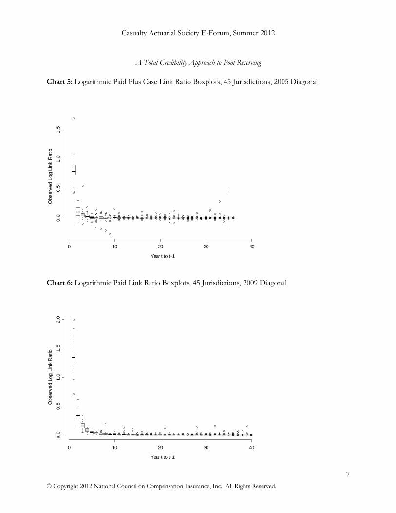
A Total Credibility Approach to Pool Reserving
Proposal 2012 Reserves Call Paper Program 7
© Copyright 2012 National Council on Compensation Insurance, Inc. All Rights Reserved.
Chart 5: Logarithmic Paid Plus Case Link Ratio Boxplots, 45 Jurisdictions, 2005 Diagonal
Chart 6: Logarithmic Paid Link Ratio Boxplots, 45 Jurisdictions, 2009 Diagonal
Year t to t+1
Obs
erve
d Lo
g Li
nk R
atio
0 10 20 30 40
0.0
0.5
1.0
1.5
Year t to t+1
Obs
erve
d Lo
g Li
nk R
atio
0 10 20 30 40
0.0
0.5
1.0
1.5
2.0
Casualty Actuarial Society E-Forum, Summer 2012

A Total Credibility Approach to Pool Reserving
Proposal 2012 Reserves Call Paper Program 8
© Copyright 2012 National Council on Compensation Insurance, Inc. All Rights Reserved.
Chart 7: Logarithmic Paid Link Ratio Boxplots, 45 Jurisdictions, 2008 Diagonal
Chart 8: Logarithmic Paid Link Ratio Boxplots, 45 Jurisdictions, 2007 Diagonal
Year t to t+1
Obs
erve
d Lo
g Li
nk R
atio
0 10 20 30 40
0.0
0.5
1.0
1.5
2.0
Year t to t+1
Obs
erve
d Lo
g Li
nk R
atio
0 10 20 30 40
0.0
0.5
1.0
1.5
2.0
Casualty Actuarial Society E-Forum, Summer 2012

A Total Credibility Approach to Pool Reserving
Proposal 2012 Reserves Call Paper Program 9
© Copyright 2012 National Council on Compensation Insurance, Inc. All Rights Reserved.
Chart 9: Logarithmic Paid Link Ratio Boxplots, 45 Jurisdictions, 2006 Diagonal
Chart 10: Logarithmic Paid Link Ratio Boxplots, 45 Jurisdictions, 2005 Diagonal
Year t to t+1
Obs
erve
d Lo
g Li
nk R
atio
0 10 20 30 40
0.0
0.5
1.0
1.5
Year t to t+1
Obs
erve
d Lo
g Li
nk R
atio
0 10 20 30 40
0.0
0.5
1.0
1.5
Casualty Actuarial Society E-Forum, Summer 2012

A Total Credibility Approach to Pool Reserving
Proposal 2012 Reserves Call Paper Program 10
© Copyright 2012 National Council on Compensation Insurance, Inc. All Rights Reserved.
3. THE STATISTICAL MODEL
At the center of the TCM is a growth curve that feeds into a double exponential likelihood. The
growth curve is motivated by the fact that logarithmic link ratios represent logarithmic rates of
growth of cumulative losses, thus resembling a biological growth process.
The three-parameter growth curve employed in the model reads:
log( ) (1 ) ( 1), , 1,..., , 0, 0 1, 0 1i iq j q j
i j i i i i iy j N q , (1)
where i indicates the state and j indicates the maturity (year); ,i jy is the (natural) logarithm of the
link ratio, and N stands for the number of observations (per state) in the data set.
The parameter delivers an estimate of the first-to-second link ratio; the parameter q is a
weighting factor between log-linear and linear influences.
All three parameters of the growth curve are subject to partial pooling. For the parameter ,
this is accomplished by means of a half-normal distribution; both the location parameter of the
parent distribution and the draws for the individual states are generated by normal distributions that
are truncated on the left at zero. For the parameter , the partial pooling of the location parameter
is implemented using beta distributions, which implies that both the location parameter of the
parent distribution and the draws for the individual states are generated by beta distributions. For
the parameter q , the location parameter of the parent distribution is again a beta distribution, but
the draws for the individual states are from a normal distribution that is left-truncated at zero and
right-truncated at unity. The use of a truncated normal (instead of a beta) distribution is motivated
by an easier convergence of the Markov chains in the Bayesian estimation process.
The growth curve stated in Equation (1) is a generalization of a functional form, the Bayesian
estimation of which has first been discussed by Gelfand and Carlin [2].
The likelihood consists of a double exponential (or, equivalently, Laplace) distribution. The
double exponential distribution is heavy-tailed and minimizes the sum of absolute errors (as
opposed to the sum of squared errors), which makes this distribution robust to outliers. Minimizing
the sum of absolute errors implies estimating the conditional median (as opposed to the traditional
approach of modeling the conditional mean). The double exponential likelihood, in its standard
form, does not account for skewness, which makes it unsuitable for studying (logarithmic) paid link
ratios.
Casualty Actuarial Society E-Forum, Summer 2012

A Total Credibility Approach to Pool Reserving
Proposal 2012 Reserves Call Paper Program 11
© Copyright 2012 National Council on Compensation Insurance, Inc. All Rights Reserved.
The precision (which is the reciprocal of the variance) of the double exponential is credibility-
adjusted. The variance of the log link ratios is allowed to vary across states. Credibility-adjusting
these variances is critical when it comes to simulating data for states that have no observations.
Further, the likelihood allows for heteroskedasticity, as the variances of the first and second log link
ratios are allowed to differ from each other and from the variance that applies to all subsequent link
ratios.
Generally, the model can be extended to accommodate more complex error structures, especially
with regards to heteroskedasticity but also with respect to the time series behavior of link ratios. For
instance, the error variance in the likelihood can be modeled as a function of the number of open
claims. Further, an autoregressive process similar to the one implemented by Meyers [6] could be
considered. However, given the sparseness of the data, such additional complexity was not deemed
desirable for annual data. Implementation of the model for quarterly data may offer additional
modeling options due to the higher number of observations.
4. RESULTS
The model is estimated by means of Markov-chain Monte Carlo simulation (MCMC). The JAGS
code of the core model is displayed in the appendix.
As mentioned, there are four states for which all link ratios are equal to unity. As a result of there
being no variation in the data for these states, the sampling process breaks down. For this reason,
the data set is jittered by adding a normally distributed error term to the logarithmic link ratios that
are equal to zero (for any state). The standard deviation of the added error term equals 0.0001.
Although the added error term is close to zero (due to the small standard deviation), in order to
have it average out to (approximately) zero, 30 jittered data sets are created and the model is run on
all of them independently. For the purpose of obtaining the posterior distributions, the codas of the
30 runs are pooled.
Three Markov chains are employed in the estimation. After a burn-in phase of 20,000 draws, 200
samples are collected per chain (from 20,000 draws per chain with a thinning parameter of 100).
The 200 samples from three chains of 30 jittered data sets then amount to 18,000 draws per
parameter. The link ratios are obtained from the logarithmic link ratio by exponentiating draw by
draw.
Casualty Actuarial Society E-Forum, Summer 2012
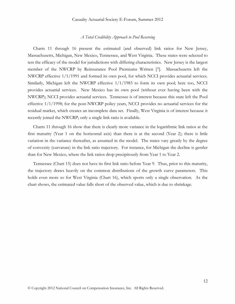
A Total Credibility Approach to Pool Reserving
Proposal 2012 Reserves Call Paper Program 12
© Copyright 2012 National Council on Compensation Insurance, Inc. All Rights Reserved.
Charts 11 through 16 present the estimated (and observed) link ratios for New Jersey,
Massachusetts, Michigan, New Mexico, Tennessee, and West Virginia. These states were selected to
test the efficacy of the model for jurisdictions with differing characteristics. New Jersey is the largest
member of the NWCRP by Reinsurance Pool Premiums Written [7]. Massachusetts left the
NWCRP effective 1/1/1991 and formed its own pool, for which NCCI provides actuarial services.
Similarly, Michigan left the NWCRP effective 1/1/1983 to form its own pool; here too, NCCI
provides actuarial services. New Mexico has its own pool (without ever having been with the
NWCRP); NCCI provides actuarial services. Tennessee is of interest because this state left the Pool
effective 1/1/1998; for the post-NWCRP policy years, NCCI provides no actuarial services for the
residual market, which creates an incomplete data set. Finally, West Virginia is of interest because it
recently joined the NWCRP; only a single link ratio is available.
Charts 11 through 16 show that there is clearly more variance in the logarithmic link ratios at the
first maturity (Year 1 on the horizontal axis) than there is at the second (Year 2); there is little
variation in the variance thereafter, as assumed in the model. The states vary greatly by the degree
of convexity (curvature) in the link ratio trajectory. For instance, for Michigan the decline is gentler
than for New Mexico, where the link ratios drop precipitously from Year 1 to Year 2.
Tennessee (Chart 15) does not have its first link ratio before Year 9. Thus, prior to this maturity,
the trajectory draws heavily on the common distributions of the growth curve parameters. This
holds even more so for West Virginia (Chart 16), which sports only a single observation. As the
chart shows, the estimated value falls short of the observed value, which is due to shrinkage.
Casualty Actuarial Society E-Forum, Summer 2012

A Total Credibility Approach to Pool Reserving
Proposal 2012 Reserves Call Paper Program 13
© Copyright 2012 National Council on Compensation Insurance, Inc. All Rights Reserved.
Chart 11: Paid Plus Case Link Ratios, New Jersey, Five Diagonals
Chart 12: Paid Plus Case Link Ratios, Massachusetts, Five Diagonals
Year t
Link
Rat
io f
rom
Yea
r t
to t
+1
_
__ _ _ _ _ _ _ _ _ _ _ _ _ _ _ _ _ _ _ _ _ _ _ _ _ _ _ _ _ _ _ _ _ _ _ _ _ _
0 10 20 30 40
1.0
1.5
2.0
2.5
_Obs. 2009 Obs. 2008 Obs. 2007 Obs. 2006 Obs. 2005 Estimated
Year t
Link
Rat
io f
rom
Yea
r t
to t
+1 _
__ _ _ _ _ _ _ _ _ _ _ _ _ _ _ _ _ _ _ _ _ _ _ _ _ _ _ _ _ _ _ _ _ _ _ _ _ _
0 10 20 30 40
1.0
1.5
2.0
2.5
3.0
_Obs. 2009 Obs. 2008 Obs. 2007 Obs. 2006 Obs. 2005 Estimated
Casualty Actuarial Society E-Forum, Summer 2012

A Total Credibility Approach to Pool Reserving
Proposal 2012 Reserves Call Paper Program 14
© Copyright 2012 National Council on Compensation Insurance, Inc. All Rights Reserved.
Chart 13: Paid Plus Case Link Ratios, Michigan, Five Diagonals
Chart 14: Paid Plus Case Link Ratios, New Mexico, Five Diagonals
Year t
Link
Rat
io f
rom
Yea
r t
to t
+1
_
_
_ _ _ _ _ _ _ _ _ _ _ _ _ _ _ _ _ _ _ _ _ _ _ _ _ _ _ _ _ _ _ _ _ _ _ _ _ _
0 10 20 30 40
1.0
1.5
2.0
2.5
3.0
_Obs. 2009 Obs. 2008 Obs. 2007 Obs. 2006 Obs. 2005 Estimated
Year t
Link
Rat
io f
rom
Yea
r t
to t
+1
_
_
_ _ _ _ _ _ _ _ _ _ _ _ _ _ _ _ _ _ _ _ _ _ _ _ _ _ _ _ _ _ _ _ _ _ _ _ _ _
0 10 20 30 40
1.0
1.5
2.0
2.5
_Obs. 2009 Obs. 2008 Obs. 2007 Obs. 2006 Obs. 2005 Estimated
Casualty Actuarial Society E-Forum, Summer 2012

A Total Credibility Approach to Pool Reserving
Proposal 2012 Reserves Call Paper Program 15
© Copyright 2012 National Council on Compensation Insurance, Inc. All Rights Reserved.
Chart 15: Paid Plus Case Link Ratios, Tennessee, Five Diagonals
Chart 16: Paid Plus Case Link Ratios, West Virginia, Five Diagonals
Year t
Link
Rat
io f
rom
Yea
r t
to t
+1
_
_
__
_ _ _ _ _ _ _ _ _ _ _ _ _ _ _ _ _ _ _ _ _ _ _ _ _ _ _ _ _ _ _ _ _ _ _ _
0 10 20 30 40
1.0
1.2
1.4
1.6
1.8
2.0
2.2
_Obs. 2009 Obs. 2008 Obs. 2007 Obs. 2006 Obs. 2005 Estimated
Year t
Link
Rat
io f
rom
Yea
r t
to t
+1 _
_
_ _ _ _ _ _ _ _ _ _ _ _ _ _ _ _ _ _ _ _ _ _ _ _ _ _ _ _ _ _ _ _ _ _ _ _ _ _
0 10 20 30 40
1.0
1.5
2.0
2.5
_Obs. 2009 Obs. 2008 Obs. 2007 Obs. 2006 Obs. 2005 Estimated
Casualty Actuarial Society E-Forum, Summer 2012

A Total Credibility Approach to Pool Reserving
Proposal 2012 Reserves Call Paper Program 16
© Copyright 2012 National Council on Compensation Insurance, Inc. All Rights Reserved.
Charts 17 through 21 provide in-sample error diagnostics for the diagonals 2009 through 2005.
The displayed residuals are standardized, thus accounting for the heteroskedasticity that has been
built into the model. There is no discernible pattern in these errors. Specifically, it appears that the
growth curve is capable of accounting for the various degrees of convexity in the link ratio
trajectories across states. Also, due to the errors being symmetric around zero along the entire
horizontal axis, the model does not systematically underpredict or overpredict at certain maturities.
Finally, the errors are not widening or narrowing in systematic ways with maturity (that is, along the
horizontal axis).
Some of the residuals are comparatively large, thus pointing to outliers in the data. This supports
the choice of a double exponential likelihood, which, due to the modeling of the conditional median
(as opposed to the mean), shows little sensitivity to outliers.
Chart 17: In-Sample Diagnostics, Paid Plus Case, 2009 Diagonal
Year t to t+1
Sta
ndar
dize
d R
esid
ual
0 10 20 30 40
-20
-10
010
20
Casualty Actuarial Society E-Forum, Summer 2012
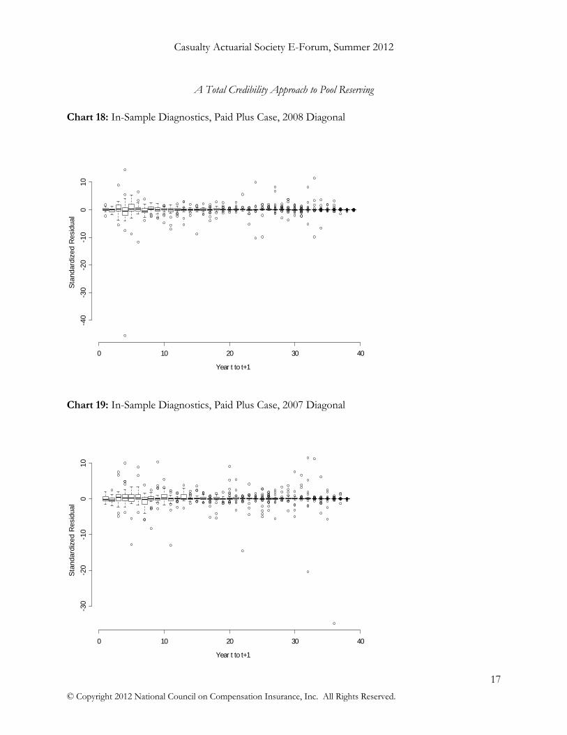
A Total Credibility Approach to Pool Reserving
Proposal 2012 Reserves Call Paper Program 17
© Copyright 2012 National Council on Compensation Insurance, Inc. All Rights Reserved.
Chart 18: In-Sample Diagnostics, Paid Plus Case, 2008 Diagonal
Chart 19: In-Sample Diagnostics, Paid Plus Case, 2007 Diagonal
Year t to t+1
Sta
ndar
dize
d R
esid
ual
0 10 20 30 40
-40
-30
-20
-10
010
Year t to t+1
Sta
ndar
dize
d R
esid
ual
0 10 20 30 40
-30
-20
-10
010
Casualty Actuarial Society E-Forum, Summer 2012

A Total Credibility Approach to Pool Reserving
Proposal 2012 Reserves Call Paper Program 18
© Copyright 2012 National Council on Compensation Insurance, Inc. All Rights Reserved.
Chart 20: In-Sample Diagnostics, Paid Plus Case, 2006 Diagonal
Chart 21: In-Sample Diagnostics, Paid Plus Case, 2005 Diagonal
Year t to t+1
Sta
ndar
dize
d R
esid
ual
0 10 20 30 40
-10
-50
510
1520
Year t to t+1
Sta
ndar
dize
d R
esid
ual
0 10 20 30 40
-10
010
20
Casualty Actuarial Society E-Forum, Summer 2012

A Total Credibility Approach to Pool Reserving
Proposal 2012 Reserves Call Paper Program 19
© Copyright 2012 National Council on Compensation Insurance, Inc. All Rights Reserved.
The model is validated using a one-year holdout period. The model is fit to the diagonals of
Calendar Years 2004 through 2008. Based on the estimated model parameters, link ratios for
Calendar Year 2009 are simulated. By comparing the simulated link ratios to the 2009 observed
values, the mean absolute forecast error is calculated. The process of model validation is
repeated using the diagonals of Calendar Years 2003 through 2007—the forecast errors are
calculated based on the observed 2008 diagonal.
Chart 22 displays the forecast errors for the 2009 diagonal; Chart 23 provides this information
for the 2008 diagonal. Clearly, in Chart 22, for the first maturity (Year 1 on the horizontal axis), the
high degree of volatility in the link ratios in these maturities leaves the median forecast error
noticeably greater than zero; this is because in that year, several states had considerably higher link
ratios in Year 1 than usual. At the same time, in Chart 23, the forecast for the link ratio at maturities
Year 1 performs considerably better. Beyond the first two maturities, the forecasts offer a high
degree of accuracy; the forecast errors are clearly symmetric.
Chart 22: Forecast Diagnostics, Paid Plus Case, 2009 Diagonal
Year t to t+1
Act
ual M
inus
For
ecas
t Lo
g Li
nk R
atio
0 10 20 30 40
-0.6
-0.4
-0.2
0.0
0.2
0.4
Casualty Actuarial Society E-Forum, Summer 2012

A Total Credibility Approach to Pool Reserving
Proposal 2012 Reserves Call Paper Program 20
© Copyright 2012 National Council on Compensation Insurance, Inc. All Rights Reserved.
Chart 23: Forecast Diagnostics, Paid Plus Case, 2008 Diagonal
5. CONCLUSIONS
The TCM is part of a family of multilevel reserving models that have recently been discussed in
actuarial literature. The model is capable of estimating not only link ratios but also delivers tail
factors. Further, the model offers credible intervals for the estimated link ratios and tail factors.
The TCM, in its current version, is not built to replicate the skewness of logarithmic paid link
ratios—thus, the model is not suitable for the analysis of paid link ratios. The use of a double-
exponential likelihood makes the estimates robust to outliers. An alternative robust likelihood is one
that rests on Student’s t distribution. This likelihood was tested on (logarithmic) paid link ratios,
using the skewed t approach developed by Kim and McCulloch [5]. The sparseness of the data
however, did not allow for a reliable identification of skewness and heavy-tailedness.
For research purposes, only annual data was used in the analysis. The model can be extended to
process quarterly (instead of annual) data. The use of quarterly data will allow for more complex
error structures, both with respect to differences across states and variation over time.
Year t to t+1
Act
ual M
inus
For
ecas
t Lo
g Li
nk R
atio
0 10 20 30 40
-0.8
-0.6
-0.4
-0.2
0.0
0.2
0.4
Casualty Actuarial Society E-Forum, Summer 2012

A Total Credibility Approach to Pool Reserving
Proposal 2012 Reserves Call Paper Program 21
© Copyright 2012 National Council on Compensation Insurance, Inc. All Rights Reserved.
6. APPENDIX
JAGS Code (Core Model)
model { #shrinkage beta.mu ~ dnorm(0,1.E-2)T(0,) beta.tau <- pow(beta.sigma,-2) beta.sigma ~ dunif(0,2) gamma.mu ~ dbeta(1,1) gamma.sigma ~ dunif(0,1) gamma.tau <- pow(gamma.sigma,-2) gamma.alpha <- gamma.mu * gamma.tau gamma.beta <- (1-gamma.mu) * gamma.tau q.mu ~ dbeta(1,1) q.sigma~ dunif(0,1) q.tau <- pow(q.sigma,-2) #q.alpha <- q.mu * q.tau #q.beta <- (1-q.mu) * q.tau for(m in 1:3){ #different variances for first two development years tau.alpha[m] ~ dexp(1.0) tau.beta[m] ~ dgamma(0.1,0.1) } #likelihood for(i in 1:L){ #rows (states) beta[i] ~ dnorm(beta.mu,beta.tau)T(0,) gamma[i] ~ dbeta(gamma.alpha,gamma.beta) q[i] ~ dnorm(q.mu,q.tau)T(0,1) #using normal instead of beta eases convergence for(m in 1:3){ tau[i,m] ~ dgamma(tau.alpha[m],tau.beta[m]) sigma[i,m] <- sqrt(2)/tau[i,m] #double exponential errors } for(j in 1:T){ #columns (development years) y.pred[i,j] ~ ddexp(mu[i,j],tau[i,tau.index[j]]) #double-indexing for tau cdf[i,j] <- sum(mu[i,j:T]) mu[i,j] <- beta[i]*pow(gamma[i],q[i]*log(j)+(1-q[i])*(j-1)) } for(j in 1:N){ #columns (development years) y.2009[i,j] ~ ddexp(mu[i,j],tau[i,tau.index[j]]) #double-indexing for tau y.2008[i,j] ~ ddexp(mu[i,j],tau[i,tau.index[j]]) y.2007[i,j] ~ ddexp(mu[i,j],tau[i,tau.index[j]]) y.2006[i,j] ~ ddexp(mu[i,j],tau[i,tau.index[j]]) y.2005[i,j] ~ ddexp(mu[i,j],tau[i,tau.index[j]]) } } }
Casualty Actuarial Society E-Forum, Summer 2012

A Total Credibility Approach to Pool Reserving
Proposal 2012 Reserves Call Paper Program 22
© Copyright 2012 National Council on Compensation Insurance, Inc. All Rights Reserved.
Acknowledgment Thanks to Dan Benzshawel, David Colón, Chris Laws, Wei Li, and Ampegama Perera for research assistance.
7. REFERENCES
[1] Carlin, Bradley P., and Thomas A. Lewis, Bayes and Empirical Bayes Methods for Data Analysis. 2nd ed., Boca Raton: Chapman & Hall/CRC, 2000.
[2] Gelfand, Alan E. and Bradley P. Carlin (1991) “An Iterative Monte Carlo Method for Nonconjugate Bayesian Analysis,” Statistics and Computing, Vol. 1, pp. 119-128.
[3] Gelman, Andrew, and Jennifer, Hill, Data Analysis Using Regression and Multilevel/Hierarchical Models, Cambridge (MA): Cambridge University Press, 2007.
[4] Guszcza, James, “Hierarchical Growth Curve Models for Loss Reserving,” Casualty Actuarial Society Forum, Fall 2008, pp. 146-173, http://www.casact.org/pubs/forum/08fforum/7Guszcza.pdf.
[5] Kim, Young Il, and J. Huston McCulloch, “The Skew‐Student Distribution with Application to U.S. Stock Market Returns and the Equity Premium,” Journal of Financial Econometrics, forthcoming.
[6] Meyers, Glenn, “Predicting Loss Ratios with a Hierarchical Bayesian Model,’’ Actuarial Review, Vol. 38, No. 1, February 2011, pp. 8-9, http://www.casact.org/newsletter/index.cfm?fa=viewart&id=6109.
[7] NCCI, Inc., Residual Market Management Summary 2010, https://www.ncci.com/Documents/RM-Mgmt-Summary-2010.pdf.
[8] Zhang, Yanwei, Vanja Dukic, and James Guszcza, “A Bayesian Nonlinear Model for Forecasting Insurance Loss Payments,” August 2010, http://www.actuaryzhang.com/publication/bayesianNonlinear.pdf.
Abbreviations and notations
IQR, Interquartile Range JAGS, Just Another Gibbs Sampler MCMC, Markov-Chain Monte Carlo SimulationNCCI, National Council on Compensation InsuranceUSL&H, United States Longshore and Harbor WorkersTCM, Total Credibility Model Biographies of the Authors Frank Schmid, Dr. habil., is a Director and Senior Economist at the National Council on Compensation Insurance, Inc.
Casualty Actuarial Society E-Forum, Summer 2012

Casualty Actuarial Society E-Forum, Summer 2012 1
Two Symmetric Families of Loss Reserving Methods
Andy Staudt, FCAS, MAAA ________________________________________________________________________
Abstract. In this paper, we introduce two families of loss reserving methods – the Actual vs. Expected family and the Mean-Reverting family. The Actual vs. Expected family can be used to credibly adjust prior expectations, either in terms of a fixed initial estimate or just a prior period’s estimate, for deviations between actual and expected experience in the same direction as the deviation. In this regard, methods within this family are useful as an alternative to a fixed a priori expectation and when rolling-forward estimates of ultimate loss. Conversely, the Mean-Reverting family can be used to credibly adjust a posteriori estimates for deviations between actual and expected experience in the opposite direction of the deviation. In this regard, methods within this family are useful in situations where either the occurrence (or absence) of events decreases (or increases) the likelihood of similar events in the future. Keywords. Reserving; Bornhuetter-Ferguson; Chain-Ladder; Benktander; Actual vs. Expected; Mean-Reversion.
1. INTRODUCTION
In this paper, we introduce two families of loss reserving methods – the Actual vs. Expected family and the Mean-Reverting family. The Actual vs. Expected family can be used to credibly adjust prior expectations, either in terms of a fixed initial estimate or just a prior period’s estimate, for deviations between actual and expected experience in the same direction as the deviation. In this regard, methods within this family are useful as an alternative to a fixed a priori expectation and when rolling-forward estimates of ultimate loss. Conversely, the Mean-Reverting family can be used to credibly adjust a posteriori estimates for deviations between actual and expected experience in the opposite direction of the deviation. In this regard, methods within this family are useful in situations where either the occurrence (or absence) of events decreases (or increases) the likelihood of similar events in the future.
Although the primary characterization and purpose of these families are different, they can be expressed generally using the symmetric formulations shown in Table 1.
Table 1. General formulations of the Actual vs. Expected and Mean-Reverting families of loss reserving methods.
Family Formulation
Actual vs. Expected (AE) Family ( )00 UpCwUU kkiAEi −+= Mean-Reverting (MR) Family ( )0UpCwUU kkiiMRi −−=
Here kp is the percentage of ultimate loss developed at time k , kC is the actual loss at time k and
iw is a weighting function.1iU We use as a generic estimate of ultimate loss using method i where
1 For the purposes of this paper, we take the development pattern and the selection of percentage to ultimate figures pk as a given rather than discuss the computation or updating of such patterns based on experience.

Two Symmetric Families of Loss Reserving Methods
Casualty Actuarial Society E-Forum, Summer 2012 2
0U is our initial expectation of ultimate and AEiU and MRiU represent the Actual vs. Expected and Mean Reverting variants of projection method i , respectively. When referring to projections of ultimate loss, we drop the time k subscript for simplicity.
To roughly understand these families, note that 0UpC kk − is an actual vs. expected adjustment as kC is the actual loss at time k and 0Upk is the amount of loss expected at time k based on our initial expectation and the loss development pattern. So, where the Actual vs. Expected family takes as its starting point our a priori expectation and credibly adjusts this amount upward for the difference between actual and expected experience to date, the Mean-Reverting family takes as its starting point our a posteriori estimate of ultimate loss and adjusts this amount downward for the difference between actual and expected experience to date.
In this regard, and considering Table 1 in detail, the symmetry of the methods is somewhat obvious. We should note, however, that this symmetry is primarily a mathematical nicety which proves useful in later sections as we derive key members and properties for each of the individual families, rather than a characteristic which intrinsically links these two families. And indeed, each of these families can be considered and used independently of one another. However, as will be discussed in Section 3.3, the Actual vs. Expected family can be used to solve a key shortcoming of the Mean-Reverting family.
1.1 Notation, Abbreviations and a Recap of Common Loss Reserving Methods Notation and abbreviations will play an important role in this paper, both to understand the
methods presented and to reflect their commonalities and lineage. For ease of reading and clarity then, it is useful to include a short but comprehensive discussion on the notation and abbreviations which will be subsequently used.
The basic notation is taken from Mack [2] with the key elements already defined above. But to recap, we define kp as the percentage of ultimate loss developed at time k , kC as the actual loss at time k , iU is the estimate of ultimate loss using loss reserving method i at time k (recall that we have dropped the k subscript for simplicity) where 0U represents the fixed a priori expectation of ultimate; and iw is a weighting function.
For the remainder of the paper, the subscript i in the term iU will be replaced with the initials of the loss reserving method used. So, for the Chain-Ladder Method we use CL, for the Bornhuetter-Ferguson we use BF and for the Gunnar-Benktander Method we use GB. We will also use the abbreviation IE, standing for Initial Expected method, and notation IEU , as well as 0U , to

Two Symmetric Families of Loss Reserving Methods
Casualty Actuarial Society E-Forum, Summer 2012 3
refer to our fixed a priori expectation of ultimate loss. The former usage is practical as it formalizes our initial expectation as a loss projection method comparable to the CL or BF method. And the latter usage is to be consistent with Mack [2] which defines the a priori expectation as the estimate at time 0=k . But also, the term 0U , indexed by the time k subscript, will become useful in later sections where we discuss rolling forward a prior period’s estimates of ultimate loss (not to be confused with the initial a priori estimate). In these cases we use the notation kU to reflect our current estimate of ultimate loss at time k and 1−kU to reflect our prior estimate of ultimate loss at time 1−k regardless of the method selected.
For each basic loss reserving method described in the preceding paragraph, the following paper will define an Actual vs. Expected variant and a Mean-Reverting variant. To differentiate the basic loss reserving methods from their variants, we will precede the subscript i in iU with AE for members of the Actual vs. Expected family and MR for members of the Mean-Reverting family. For instance, we will use the abbreviation AEBF and the notation AEBFU to refer to the Actual vs. Expected Bornhuetter-Ferguson method and the abbreviation MRBF and the notation MRBFU to refer to the Mean-Reverting Bornhuetter-Ferguson method.
1.2 Common Loss Reserving Methods and the Experience Adjusted Method As a refresher, Table 2 below shows the calculations underlying each of the basic loss reserving
methods used in this paper with both the traditional as well as the credibility formulations shown to highlight the relationships between these methods. Table 2. Notation and formulations of common loss reserving methods as well as the Experienced Adjusted method.
Abbrev. Name Traditional Formulation Credibility Formulation
IE Initial Expected 0UU IE = N/A
EA Experience Adjusted ( )00 UpCpUU kkkEA −+= ( ) 01 UpUp kBFk −+=
BF Bornhuetter-Ferguson 0)1( UpCU kkBF −+= ( ) 01 UpUp kCLk −+=
GB Gunnar Benktander ( ) BFkkGB UpCU −+= 1 BFkCLk UpUp )1( −+=
CL Chain-Ladder k
kCL p
CU = N/A
While the IE, CL, BF, and GB methods should be familiar to most actuaries, this paper introduces a new method which we call the Experience Adjusted method, denoted using EA. The EA method, although to the best of our knowledge not defined in the actuarial literature, is useful for presenting an evenly-spaced spectrum of potential members of the Actual vs. Expected and

Two Symmetric Families of Loss Reserving Methods
Casualty Actuarial Society E-Forum, Summer 2012 4
Mean-Reverting families; and is defined as
( )00 UpCpUU kkkEA −+= . (1)
Where the CL and IE methods are polar opposites, and the BF method is the credibility-weighted average of these two methods, the EA method is the polar opposite of the GB method. To understand this note that the GB method can be expressed as the credibility weighted average of the BF and CL methods as shown in Table 2 or Mack [2], whereas the EA method can be expressed as the credibility-weighted average of the BF and IE methods. Working backwards, we shows this as
( ) ( )[ ] ( )( ) ( )
( )( )( )
( )EA
kkk
kkk
kkk
kkkk
kkkkk
kkkkkBFk
UUpCpU
UpUCpUpCp
UppCpUpUppCp
UpUpCpUpUp
=−+=−+=
−+=−++=
−+−+=−+−+=−+
00
02
0
02
0
00
000
111
11111
(2)
And thus, these five methods – the IE, EA, BF, GB, and CL – form a spectrum from no credibility to full credibility with respect to current experience.
1.3 Outline The remainder of the paper is structured as follows. In Section 2 we present the Actual vs.
Expected family and in Section 3 we present the Mean-Reverting family. Generally these sections follow the same outline where we first present the general formulation of the family and then discuss the family’s “generator function” which is used to derive specific members of that family. We then discuss considerations when selecting a specific member of each family before focusing on the practical uses of each family and note any contra-indications. We will also introduce extensions to the basic versions of these families as defined in Table 1. In Section 2, we introduce the Generalized Actual vs. Expected family which can be used to roll forward prior estimates of ultimate loss. And in Section 3, we introduce the Adjusted Mean-Reverting family which corrects for a flaw in the basic version of the Mean-Reverting family. Finally, in Section 3, we also comment upon the relative accuracy of the Mean-Reverting family using hindsight testing. The conclusion of this paper highlights the four members of these families which might prove most useful to the actuary in a practical setting. We also include an Appendix which discusses the motivation for this paper (Appendix A) and attach an Excel file which shows how to implement these methods (Appendix B).

Two Symmetric Families of Loss Reserving Methods
Casualty Actuarial Society E-Forum, Summer 2012 5
2. THE ACTUAL VS. EXPECTED FAMILY
In this section, we focus on the Actual vs. Expected family. This family can be used to credibly adjust prior expectations, either in terms of a fixed initial estimate or just a prior period’s estimate, for deviations between actual and expected experience in the same direction as the deviation. In this regard, methods within this family are useful as an alternative to a fixed a priori expectation and when rolling forward estimates of ultimate loss.
2.1 General Formulations
2.1.1 The actual vs. expected formulation
As discussed above, the Actual vs. Expected family is defined as
( )00 UpCwUU kkiAEi −+= . (3)
Without any loss of generality, Equation (3) can be used to develop any data triangle (i.e., paid or incurred losses as well as reported or closed claim counts). For the purpose of understanding this family, note that 0UpC kk − is an actual vs. expected adjustment as kC is the actual loss at time k and 0Upk is the amount of loss expected at time k based on our initial expectation and the loss development pattern. For example, if actual losses are more than expected, this family would adjust the initial expectation upward allowing for some portion, iw , of this deviation, and vice versa.
From this interpretation, it is obvious that the critical factor is the weighting function iw which determines the amount of reliance we place on the actual vs. expected adjustment relative to initial expectations. If we were to set 1=iw , then we would adjust the a priori expectation fully for the deviation between actual and expected experience. On the other hand, if we were to set 0=iw , then Equation (3) would reduce to the a priori expectation, ignoring actual experience. This loosely suggests that the weighting function iw can be viewed as the credibility of the actual vs. expected adjustment and that an acceptable constraint is ]1,0[∈iw .
Consider the following example. Suppose that the historical percentage of loss developed at time k is 25%, the initial expectation of ultimate is $200, and the current loss amount is $150. In Equation (3), suppose that we set the weighting factor equal to the percentage of loss developed at time k (i.e., ki pw = ). As will be shown in the next section, this is actually a special case of the Actual vs. Expected family – namely the Actual vs. Expected Bornhuetter-Ferguson (AEBF) method. Table 3 below compares our fixed initial expectation against the AEBF method. From this comparison, we see that as actual losses were $100 more than expected ($150 less 25% of $200), but only 25% credible according to the weighting function defined above, we only adjust our initial

Two Symmetric Families of Loss Reserving Methods
Casualty Actuarial Society E-Forum, Summer 2012 6
expectation upward by $25 (25% of 100).
Table 3. Simple example comparing IE method with the AEBF method.
IE Method AEBF Method
2000
== UU IE
( )( )
225100%25200
200%25150%2520000
=×+=
×−×+=−+= UpCpUU kkkAEBF
2.1.2 The credibility formulation
Even restricting ]1,0[∈iw , there are still an infinite number of members of the Actual vs. Expected family, which, practically, isn’t a very useful result. Rather, it is more constructive to limit ourselves to a finite subset of the family. One or two methods which could be used regularly during a reserve review. To this end, consider the following credibility formulation:
0)1( UpUpU kikAEi −+= . (4)
Equation (4) takes the standard form of credibility-weighted averages defined in the actuarial literature (see Mahler and Dean [3]) where we use kp to weight together our “observation” iU based on experience with our initial estimate 0U based on “other information.” Although it is not immediately obvious, this credibility equation defines a subset of members of the Actual vs. Expected family. Similar to the moment or probability generating functions in statistics, this equation can be used as a “generator function” for the Actual vs. Expected family, where, by inserting common loss reserving methods into the iU term, the resulting formula (rearranged) returns a member of this family.
For example, suppose we were to insert the BF method into Equation (4). Then we can derive what we will call the AEBF method as
[ ]
( )00
002
0002
0
00
0
0
)1()1()1(
)1(
UpCpUUUpCp
UpUUpUpCpUpUpCp
UpUpUUpUpU
kkk
kkk
kkkkk
kkkk
kBFkAEBF
kikAEi
−+=+−=
−+−+=−+−+=
−+=−+=
(5)
Or, to show another derivation, consider inserting the EA method into Equation (4) to derive what we will call the AEEA method as

Two Symmetric Families of Loss Reserving Methods
Casualty Actuarial Society E-Forum, Summer 2012 7
( )[ ]
( )02
0
0032
00032
0
000
0
0
)1()1(
)1(
UpCpUUUpCp
UpUUpCpUpUpUpCpUp
UpUpUUpUpU
kkk
kkk
kkkkk
kkkkk
kEAkAEEA
kikAEi
−+=+−=
−+−+=−+−+=
−+=−+=
(6)
Table 4 below presents three other distinct members of this family, along with the AEBF and AEEA methods, which were all derived in a similar manner – by inserting the named loss reserving method into the generator function in Equation (4) and rearranging. Table 4 also explicitly presents the weight function which defines each of these methods within the actual vs. expected formulation. This function reflects weight or credibility each method gives the actual vs. expected adjustment, with the AEIE method placing no weight on the adjustment and the AEEA, AEBF, AEGB, and AECL methods placing increasing weight on actual relative to expected experience.
Table 4. Members of the Actual vs. Expected family of loss reserving methods differentiated by their weight function.
Method Credibility Formulation Actual vs. Expected Formulation Weight Function
AEIE 0)1( UpUpU kIEkAEIE −+= ( ) IEkkAEIE UUpCUU ⇒−+= 00 0 0 AEEA 0)1( UpUpU kEAkAEEA −+= ( )0
20 UpCpUU kkkAEEA −+= 2
kp AEBF 0)1( UpUpU kBFkAEBF −+= ( ) EAkkkAEBF UUpCpUU ⇒−+= 00 kp AEGB 0)1( UpUpU kGBkGB −+= ( )( )0
20 2 UpCppUU kkkkAEGB −−+= 22 kk pp −
AECL 0)1( UpUpU kCLkAECL −+= ( ) BFkkAECL UUpCUU ⇒−+= 00 1 1
The table above begins to indicate an important relationship. Namely, the Actual vs. Expected family is fundamentally a generalization of the BF method. Table 5 below illustrates this by placing the credibility formulation of the Actual vs. Expected family as defined in Equation (4) next to the credibility formulation of the BF method. Rather than restricting our “observation” within the credibility formula to the CL method, the Actual vs. Expected family lets us use any alternative method. In fact, we note that if we use the BF method as our plug-in estimator, than the resultant Actual vs. Expected variant is the EA method discussed in Section 1.2.
Table 5. Comparison of the Actual vs. Expected family and the BF method.
Family Formulation
Credibility Formulation of Actual vs. Expected Family 0)1( UpUpU kikAEi −+= Bornhuetter-Ferguson Method ( ) 01 UpUpU kCLkBF −+=
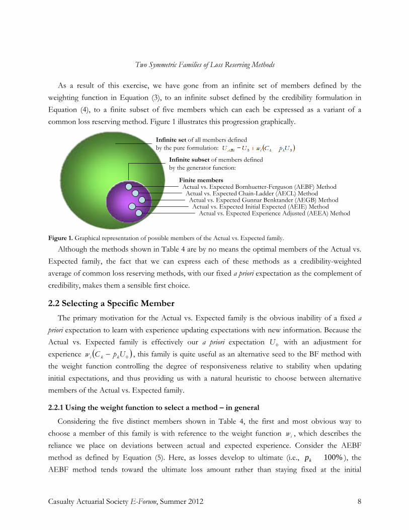
Two Symmetric Families of Loss Reserving Methods
Casualty Actuarial Society E-Forum, Summer 2012 8
As a result of this exercise, we have gone from an infinite set of members defined by the weighting function in Equation (3), to an infinite subset defined by the credibility formulation in Equation (4), to a finite subset of five members which can each be expressed as a variant of a common loss reserving method. Figure 1 illustrates this progression graphically.
Actual vs. Expected Bornhuetter-Ferguson (AEBF) MethodActual vs. Expected Chain-Ladder (AECL) MethodActual vs. Expected Gunnar Benktander (AEGB) MethodActual vs. Expected Initial Expected (AEIE) Method
Actual vs. Expected Experience Adjusted (AEEA) Method
Infinite set of all members defined by the pure formulation:
Infinite subset of members defined by the generator function:
Finite members…
Figure 1. Graphical representation of possible members of the Actual vs. Expected family.
Although the methods shown in Table 4 are by no means the optimal members of the Actual vs. Expected family, the fact that we can express each of these methods as a credibility-weighted average of common loss reserving methods, with our fixed a priori expectation as the complement of credibility, makes them a sensible first choice.
2.2 Selecting a Specific Member The primary motivation for the Actual vs. Expected family is the obvious inability of a fixed a
priori expectation to learn with experience updating expectations with new information. Because the Actual vs. Expected family is effectively our a priori expectation 0U with an adjustment for experience ( )0UpCw kki − , this family is quite useful as an alternative seed to the BF method with the weight function controlling the degree of responsiveness relative to stability when updating initial expectations, and thus providing us with a natural heuristic to choose between alternative members of the Actual vs. Expected family.
2.2.1 Using the weight function to select a method – in general
Considering the five distinct members shown in Table 4, the first and most obvious way to choose a member of this family is with reference to the weight function iw , which describes the reliance we place on deviations between actual and expected experience. Consider the AEBF method as defined by Equation (5). Here, as losses develop to ultimate (i.e., %100→kp ), the AEBF method tends toward the ultimate loss amount rather than staying fixed at the initial

Two Symmetric Families of Loss Reserving Methods
Casualty Actuarial Society E-Forum, Summer 2012 9
expectation. Now, in this instance, we do not apply the full actual vs. expected adjustment, rather the rate at which we adjust the a priori expectation for actual experience is commensurate with the percentage of loss developed ki pw = at time k .
Figure 2 below illustrates the weight each of the defined Actual vs. Expected methods place on the actual vs. expected adjustment as a function of the amount of developed experience.
0%
10%
20%
30%
40%
50%
60%
70%
80%
90%
100%
0% 10% 20% 30% 40% 50% 60% 70% 80% 90% 100%
Percentage Developed
Wei
ght o
n A
ctua
l vs.
Exp
ecte
d A
djus
tmen
t
Actual vs. Expected Chain-Ladder (AECL)
Actual vs. Expected Gunnar Benktander (AEGB)
Actual vs. Expected Bornhuetter-Ferguson (AEBF)
Actual vs. Expected Experience Adjusted (AEEA)
Actual vs. Expected Initial Expected (AEIE)
Figure 2. The weight these members of the Actual vs. Expected family give the actual vs. expected adjustment.
From this illustration, we can see that the AEGB method is more responsive than the AEEA method. As was discussed in Section 1.1, this makes sense, given that the GB method places more weight on developed experience than the EA method which places more weight on the initial expectation. And the AEBF method, as with its namesake, takes the middle ground and places “equal” weight on the actual vs. expected adjustment as on the a priori expectation. In contrast, the AECL method makes a full allowance for the actual vs. expected adjustment.
Or, presented another way, return for a moment to the previous example (i.e., the percentage developed at time k is 25%, the initial expectation is $200, and the current loss amount is $150). Table 6 shows the estimate of ultimate loss in this example using each of the five defined Actual vs. Expected methods. Note that we have also explicitly specified the weight given to developed experience as a means of indicating the relative responsiveness / stability of each method.

Two Symmetric Families of Loss Reserving Methods
Casualty Actuarial Society E-Forum, Summer 2012 10
Table 6. Projections of ultimate loss using various members of the Actual vs. Expected family.
Method Ultimate Loss Projection Weight Function
AEIE ( )00 0 UpCUU kkAEIE −+= = 00.200$ 0=IEw = %00.0 AEEA ( )0
20 UpCpUU kkkAEEA −+= = 25.206$ 2
kEA pw = = %25.6 AEBF ( )00 UpCpUU kkkAEBF −+= = 00.225$ kBF pw = = %00.25 AEGB ( )( )0
20 2 UpCppUU kkkkAEGB −−+= = 75.243$ 22 kkGB ppw −= = %75.43
AECL ( )00 1 UpCUU kkAECL −+= = 00.300$ 1=CLw = %00.100
2.2.2 Using the weight function to select a method – more specifically
While there is not a most accurate member of the Actual vs. Expected family, it is useful to take a position. For the moment, let us consider the AEBF, as the weight it gives to the difference between actual and expected losses is directly proportionate to the amount of experience, so that neither prior expectations nor actual relative to expected losses are unduly favored.
Or, put another way, actuaries will be familiar with actual vs. expected diagnostics which compare the change in ultimate to actual less expected experience. In these diagnostics, if the actuary is using the BF method, the change in ultimate will perfectly mirror the actual vs. expected statistic. Or if the actuary is pegging loss to a prior or initial estimate, then the change in ultimate will be zero regardless of actual experience. However, as is very often the case when reviewing these diagnostics, the change in ultimate generally lies somewhere between zero and the actual vs. expected statistic indicating that partial credibility has been given to actual vs. expected experience in the period. This makes sense, given that actuaries will often select an estimate of ultimate loss based on not just one projection method but a variety of methods utilizing averaging, rounding, and potentially manual adjustments to the methods where necessary. To this end, the Actual vs. Expected family is useful for formalizing the results of these diagnostics into a projection method, where at one extreme, the diagnostic is ignored, and, at the other extreme, the diagnostic is believed. And in between, the diagnostic is given a degree of credibility proportional to the amount of experience in the period.
In the case of the AEBF method, using the percentage of expected loss development in the period kp as the degree of credibility seems like a natural and sensible choice. Note that this construction allows the credibility we place on actual loss experience to be linearly proportional to our expectation of loss emergence over the same period.
2.3 The Generalized Actual vs. Expected Family Alternatively, a natural use of the Actual vs. Expected family arises when rolling forward prior

Two Symmetric Families of Loss Reserving Methods
Casualty Actuarial Society E-Forum, Summer 2012 11
actuarial work. Consider the situation where full reserve reviews are done periodically (perhaps annually or quarterly) and actual vs. expected diagnostics are used in the interim to adjust for experience over the period. Most often, actuaries tend to one extreme or the other and either allow for 100% of the experience in the period (as updating estimates of ultimate loss using the BF method would) or make no adjustment for the experience in the period (as fixing estimates of ultimate loss at prior selections would). In the case of the former instance, the change in ultimate would exactly mirror the actual vs. expected statistic, and in the case of the latter, the change in ultimate would be zero regardless of the actual vs. expected statistic.
In these situations, given the all-or-nothing nature of movements over what are potentially short and not fully credible time intervals, it is perhaps more useful to first assess the credibility of experience in the period and then adjust our estimates of ultimate as such. Hopefully, this process more appropriately balances the need for responsiveness with the need for stability, or at least provides a formalized means of doing so. Equation (7) generalizes the AEBF method for exactly this purpose – to string together estimates of ultimate loss in subsequent development periods controlling for the random volatility vs. credibility of loss emergence within relatively short intervals. We call this method the Generalized Actual vs. Expected Bornhuetter-Ferguson method or the GAEBF method.
( ) ( )
−
−−
−−
−−
+== −−−
−−
−
−− 11
1
11
1
11 11 kk
k
kkkk
k
kkkkGAEBF CU
ppp
CCppp
UUU (7)
Here the subscript k refers to the current period and the subscript 1−k refers to the prior period. Note that for development from time 0=k where 01 =−kp , 01 UUk =− and 01 =−kC , Equation (7) reduces to the AEBF method described in Equation (5). And as with Equation (5), this projection method adheres to the general principle that the longer the period over which actual experience is measured, the more weight given to actual experience relative to prior expectations, either with regard to a prior estimate or an initial expectation.
To help understand how the AEBF method works in this situation, it is useful to further develop the simple example of the previous section. Suppose that one month has elapsed since our previous actuarial review where we ended up selecting $225 (i.e., the amount as projected under the AEBF method) and the incurred loss amount is now $195 (i.e., actual incurred in the period of $45) and the percentage developed is now 40% (i.e., expected percentage developed in the period of 15%). From Equation (7), we can roll forward our prior estimate of ultimate loss of $225 as

Two Symmetric Families of Loss Reserving Methods
Casualty Actuarial Society E-Forum, Summer 2012 12
( ) ( )
( ) ( )
( )( )
2316225
1545%2022575%2045%20225
150225%251
%25%40150195
%251%25%40
225
11 111
11
1
11
=+=
−+=×−+=
−
−−
−−
−−
+=
−
−−
−−
−−
+= −−−
−−
−
−− kk
k
kkkk
k
kkkk CU
ppp
CCppp
UU
(8)
Actual development in the period was $45 and expected development was 20% of the unreported amount of $75, or $15; thus, the actual vs. expected adjustment is $30. However, as this was a short period with only 20% expected development on unreported, we only adjust the ultimate loss amount by 20% of total implied adjustment, or $6, for an ultimate of $231. Note that the degree of credibility depends both on the length of the period as well as the shape of the paid or incurred development patterns.
2.4 Contra-Indications With regard to using a member of the Actual vs. Expected family in either of the situations listed
above, there aren’t necessarily any obvious contra-indications.
In the former instance, when using a non-trivial member of the Actual vs. Expected family as an alternative to a fixed a priori expectation, this family will often be preferable to fixing an initial expectation and failing to update this expectation as more evidence becomes available. Additionally useful, this family allows the actuary to determine the extent to which they wish to peg their a priori estimate to initial expectations with the AEEA being the most sticky and the AEGB being the most aggressive (ignoring the trivial case of the AEIE method).
Similarly, in the latter instance, when using a non-trivial member of the Generalized Actual vs. Expected family to roll-forward prior estimates, it is perhaps more a judgment call (rather than a case of selecting a “most accurate” method) when deciding between allowing for 0% of the actual vs. expected experience as is true of fixing estimates of ultimate loss at prior selections, 100% of actual vs. expected experience as is the case with updating BF projections or somewhere in the middle taking into consideration the credibility of experience over the time interval. In any event, this approach should provide the actuary with more freedom when it comes to balancing responsiveness and stability.

Two Symmetric Families of Loss Reserving Methods
Casualty Actuarial Society E-Forum, Summer 2012 13
3. THE MEAN-REVERTING FAMILY
This section introduces the Mean-Reverting family of loss reserving methods. As the doppelganger of the Actual vs. Expected family, the Mean-Reverting family can be used to credibly adjust a posteriori estimates for deviations between actual and expected experience in the opposite direction of the deviation. In this regard, methods within this family are useful in situations where the occurrence of events decreases the likelihood of similar events in the future, or likewise, when the absence of events increases the likelihood of similar events in the future.
Put another way, this family effectively relaxes the independence assumption of the BF method and the positive dependence assumption of the CL method and allows for the potential of some negative dependence between current and future losses.
3.1 General Formulations
3.1.1 The actual vs. expected formulation
Similar to the Actual vs. Expected family, members of the Mean-Reverting family are grounded in an actual vs. expected adjustment. However, where in respect of the Actual vs. Expected family, the adjustment is used to fine-tune a priori expectations for actual experience, in respect of the Mean-Reverting family, the adjustment is used to bring a posteriori projections back toward some long-run estimate of the mean. Mathematically, this is formulated as
( )0UpCwUU kkiiMRi −−= . (9)
To understand the name and purpose of the Mean-Reverting family, note that through some simple manipulations (adding and subtracting kC ) we can rearrange Equation (9) as
( ) ( )[ ]0UpCwCUCU kkikikMRi −−−+= . (10)
This arrangement is useful as it isolates both the unadjusted and adjusted outstanding reserve, ( )ki CU − and ( ) ( )[ ]0UpCwCU kkiki −−− , respectively, from the current amount of loss kC . In doing so, it becomes clear that the Mean-Reverting family offsets the unadjusted outstanding reserve for the amount by which actual losses deviated from expected losses (subject to some weight iw ). For example, if losses to date were more than expected, the outstanding reserve would be decreased to reflect the propensity for future losses to be less than expected, and vice versa. It is this type of “mean-reversion” from which the name of the family is derived.
To understand the mechanics of this family, we return again to the simple example from the previous section. Remember that the percentage developed is 25%, current incurred loss is $150,

Two Symmetric Families of Loss Reserving Methods
Casualty Actuarial Society E-Forum, Summer 2012 14
and our initial expectation of ultimate is $200. In Equation (9), assume that we are using the BF method as our unadjusted estimate of ultimate loss (i.e., BFi UU = and MRBFMRi UU = ) and set the weighting factor equal to the percentage developed at time k (i.e., kk pw = ). As will be shown in the next section, this is actually a special case of the Mean-Reverting family – namely the Mean-Reverting Bornhuetter-Ferguson (MRBF) method. From Table 7, which compares the BF method with its Mean-Reverting variant, we see that as actual losses were more than expected, the MRBF method adjusts the BF outstanding reserve/ultimate liability downward back toward initial expectations allowing for a degree of mean-reversion over the future experience period.
Table 7. Simple example comparing BF method with the MRBF method.
BF Method MRBF Method
300200%)251(150
)1( 0
=×−+=
−+= UpCU kkBF
( )
( )
275100%25300
200%25150%253000
=×−=
×−×−=−−= UpCpUU kkkBFMRBF
Here, although the difference between actual and expected experience is $100, we only adjust the BF projection by 25% of this amount representing the credibility we assign the degree of mean-reversion. It is this weight, as well as the basis of the a posteriori projection, which distinguishes members of the Mean-Reverting family. We explore the link between these two components in the next section.
3.1.2 The credibility formulation2
Similar to as was done with the Actual vs. Expected family, we can define a generator function for the Mean-Reverting family that isolates a subset of this family and expresses these members as the credibility-weighted average of the fixed a priori expectation and the unadjusted loss reserving method. This generator function is shown below in Equation (11). What is immediately obvious, and to some extent reasonable, given the relationship between the Actual vs. Expected and Mean-Reverting families, is that this formulation is the mirror opposite of the credibility formulation of the Actual vs. Expected family.
ikkMRi UpUpU )1(0 −+= (11) 2 Technically, the generator function formulation presented in Equation (11) is the opposite of a credibility-weighted projection where the estimate of ultimate loss tends toward the complement of credibility U0 and away from experience as losses develop to ultimate. This is obviously not ideal and will be addressed Section 3.3, where we present an adjusted version of this family which tends toward experience and away from prior expectations as losses develop to ultimate.

Two Symmetric Families of Loss Reserving Methods
Casualty Actuarial Society E-Forum, Summer 2012 15
Using the same basic loss reserving methods as above, Table 8 shows both the actual vs. expected and credibility formulations of the Mean-Reverting variants for the IE, EA, BF, GB, and CL methods. As in Section 2, each of these methods were derived by plugging the unadjusted method into the generator function in Equation (11) and solving for the weight in the pure formulation shown in Equation (9).
Table 8. Five members of the Mean-Reverting family of loss reserving methods.
Method Credibility Formulation Actual vs. Expected Formulation Weight Function
MRIE IEkkMRIE UpUpU )1(0 −+= )(0 0UpCUU kkIEMRIE −−= 0 MREA EAkkMREA UpUpU )1(0 −+= )( 0
2 UpCpUU kkkAEMREA −−= 2kp
MRBF BFkkMRBF UpUpU )1(0 −+= )( 0UpCpUU kkkBFMRBF −−= kp MRGB GBkkMRGB UpUpU )1(0 −+= ))(2( 0
2 UpCppUU kkkkGBMRGB −−−= 22 kk pp − MRCL CLkkMRCL UpUpU )1(0 −+= )(1 0UpCUU kkCLMRCL −−= 1
There are two items of interest concerning Table 8. The first is that the method which is plugged into the generator function in Equation (11) is the same method which is used as the a posteriori projection in the actual vs. expected formulation. This is useful, as it reduces the complexity of this family from two free parameters (the a posteriori projection and the weight given the actual vs. expected adjustment) to a single free parameter (the a posteriori projection) which fully defines members of this family. The second is that the weights given to the actual vs. expected (or mean-reverting) adjustments are identical to the weights given the adjustments in the Actual vs. Expected family; however, the starting points, the a priori expectation in terms of the Actual vs. Expected family and the a posteriori estimates in terms of the Mean-Reverting family, are different. We explore this symmetry in the next section.
3.2 Selecting a Specific Member
3.2.1 The notion of relative mean-reversion
For completeness, in Table 8 we also show the trivial case of the MRIE, noting that this method reduces to the a priori expectation. This is useful, as it highlights that members of the Mean-Reverting family, as with the Actual vs. Expected family, form a spectrum from 0 to 100% weight on the actual vs. expected adjustment.
With that said, it is important when interpreting these methods that the weight given the actual vs. expected adjustment is not mistaken for the degree of mean-reversion. In contrast to the Actual vs. Expected family, where each method applies a different adjustment to the same starting point

Two Symmetric Families of Loss Reserving Methods
Casualty Actuarial Society E-Forum, Summer 2012 16
(i.e., the a priori expectation), each member of the Mean-Reverting family applies a different adjustment to a different starting point (i.e., the chosen a posteriori estimator). In this regard, each member of the Mean-Reverting family should primarily be considered in relation to its unadjusted variant, rather than with respect to other actuarial methods or some absolute reference.
To explore this concept further, we define the coefficient of mean-reversion as
0UUUU
Ci
MRiiMRi −
−= . (12)
To understand this equation, note that the denominator expresses the amount by which the unadjusted method deviates from our a priori expectation and the numerator expresses the amount by which the Mean-Reverting variant of the unadjusted method pulls the answer back toward the mean or initial expectation.
We derive the coefficient of mean-reversion for the MRBF and MRCL methods in Table 9.
Table 9. Derivation of coefficient of mean-reversion for MRBF and MRCL methods.
MRBF Coefficient of Mean-Reversion MRCL Coefficient of Mean-Reversion
( )[ ]( )
( )
k
kk
kkk
kk
kkkBFBF
BF
MRBFBFMRBF
pUpC
UpCpUpUC
UpCpUUUU
UUC
=−−
=
−−+−−−
=
−−
=
0
0
00
0
0
1 ( )[ ]
( )( )
k
kkk
kk
kk
kkCLCL
CL
MRCLCLMRCL
ppUpC
UpCUpC
UpCUUUU
UUC
=−−
=
−−−−
=
−−
=
/
/1
0
0
0
0
0
Note that the coefficient of mean-reversion is the same for both these methods. And indeed, using this definition, we can easily demonstrate that the relative mean-reversion for each of the Mean-Reverting methods shown in Table 8 (or derived via Equation (11)) will always be equivalent and equal to the percentage developed kp at time k . This makes intuitive sense, given that the mean to which the ultimate loss reverts in Equation (11) is our a priori expectation and the credibility assigned to this initial expectation is kp .
3.2.2 The notion of absolute mean-reversion
Although each member of the Mean-Reverting family introduces the same degree of mean-reversion relative to its unadjusted variant, this does not necessarily imply that each method has the same absolute mean-reversion. Rather, the absolute mean-reversion of the family (i.e., the degree of negative dependence between current and future losses) depends not just on the mean-reverting

Two Symmetric Families of Loss Reserving Methods
Casualty Actuarial Society E-Forum, Summer 2012 17
adjustment, but also on the degree of dependence between current and future losses in the underlying method. For instance, consider the BF and CL methods. Where the BF method assumes that future losses are independent of losses to date, the CL method assumes a large degree of positive dependence between current and future losses with the unearned reserve leveraged for experience to date.
We can demonstrate this roughly by considering a slightly unusual version of the outstanding reserve ( )ki CU − for each of these methods as shown in Table 10.
Table 10. Comparison of the CL and BF estimates of the outstanding reserve.
Method Outstanding Reserve Dependence
CL Method ( ) ( )001
1 UpCp
ppU kk
k
kk −
−+− Positivepk ⇒∈ ]1,0(
BF Method ( ) ( )( )00 01 UpCpU kkk −+− tIndependenpk ⇒∈ ]1,0(
Here we split the outstanding reserve into two components – the “independent” reserve ( )kpU −10 which bears no relationship to loss experience kC and the “dependent” reserve ( )0UpC kk − which is the actual vs. expected adjustment. This is a useful formulation, as we can easily assess the dependence of the outstanding reserve on experience to date. For the BF method, as the dependent reserve is zero, this method assumes future loss experience is fully independent of current loss experience. But for the CL method, as the independent reserve adjustment factor ( ) kk pp /1− is always positive, the CL method assumes that future loss experience is positively dependent on current loss experience adjusting the independent reserve upward.
Now consider Table 11 which shows a similar comparison for the MRCL and MRBF methods.
Table 11. Comparison of the MRCL and MRBF estimates of the outstanding reserve.
Method Outstanding Reserve Dependence
MRCL Method ( ) ( )0021
1 UpCp
ppU kk
k
kk −
−+−
⇒⇒⇒
∈Negative
tIndependenPositive
pk
]1,5.0(5.0
)5.0,0(
MRBF Method ( ) ( )( )00 1 UpCppU kkkk −−− { Negativepk ⇒∈ ]1,0(
Here it becomes evident that while each Mean-Reverting method does introduce some negative dependence or mean-reversion into its unadjusted variant, the final absolute dependence between future and current loss experience is not necessarily negative. Rather it depends on the interaction between the dependence of future and current loss experience in the underlying method and the

Two Symmetric Families of Loss Reserving Methods
Casualty Actuarial Society E-Forum, Summer 2012 18
strength of the mean-reversion adjustment.
For the MRBF method, because the underlying BF method assumes that current and future loss experience is independent, applying a mean-reverting adjustment to this method will obviously produce estimates of the outstanding reserve which are negatively dependent on experience to date. And from Table 11 we can see that, at all stages of loss development, this is indeed the case. For the MRCL method, however, the result is a little bit trickier, as the CL estimate of the outstanding reserve is positively dependent on losses to date. Thus, the absolute degree of mean-reversion depends on the interaction between the credibility given the negative dependence in the mean-reverting adjustment and the credibility given the positive dependence in the CL method. Specifically, when %50<kp , the positive dependence of the CL method dwarfs the mean-reversion adjustment and the estimate of the outstanding liability is still positively dependent on experience to date (however, less so than with the CL method). When %50>kp , the mean-reversion adjustment is more influential than the leveraged effect of the CL projection and the estimate of the outstanding liability is negatively dependent on experience to date. And when %50=kp , there is balance and the estimate of the outstanding liability and experience to date are largely independent.
The summation of these two sections implies that there are two layers of interpretation regarding the Mean-Reverting family. The first is that each member of the Mean-Reverting family introduces a relative degree of mean-reversion into its underlying variant. The second is that the absolute mean-reversion in the final result depends on the relationship between the underlying method chosen and the credibility given the mean-reversion adjustment. This is a useful result, as these two interpretations begin to hint at a two-step procedure for selecting a member of the Mean-Reverting family. First, select a best unadjusted method, and then, if the situation warrants, adjust that method for some degree of mean-reversion. This is discussed in the next section and will be illustrated using actual data in Section 3.4.
3.2.3 Putting it all together
As mentioned above, the Mean-Reverting family is most useful in situations where either the occurrence or the absence of an event has the opposite impact on the likelihood of similar events in the future. These situations arise when reserving for a variety of lines characterized by total / near-total losses or some notion of risk aging or mortality. Such examples might include marine, crop, credit disability, construction defect, and extended warranty.
For instance, consider an extended warranty policy. As the policy ages, the loss potential generally

Two Symmetric Families of Loss Reserving Methods
Casualty Actuarial Society E-Forum, Summer 2012 19
increases with product wear and tear. And, although we may try to take this into account through our earning pattern, if losses to date are less than expected, it may become necessary to make an adjustment for the increased future loss propensity given the weighted aging of the account. Conversely, if losses are more than expected, then it may become necessary to reduce the future possibility of losses, as policies either exit the portfolio or the products are replaced with newer versions and the weighted age of the account decreases.
When deciding whether to use, say, the BF or CL method or their mean-reverting variants, it is useful to query why actual losses were more or less than expected. Continuing with the example of extended warranty insurance, suppose that there is no discernable reason why losses were more than expected. In this case, we are implying that, although losses were more than expected, we do not expect such trends to continue. Here the BF method is potentially more useful than the CL method, as the estimate of the outstanding liability is independent of current experience to date. However, although losses were more than expected, we might reasonably expect some degree of mean-reversion associated with the replacement of products, and the MRBF method is potentially more useful than the BF method.
On the other hand, suppose that losses were more than expected due to a “catastrophe” event such as a substantial product defect. In this case, the CL method is probably more useful than the BF method, as we should probably expect a higher number of future losses because of the defect. However, in this situation there is still potentially a degree of mean-reversion associated with the policy exit or product replacement decreasing the future propensity to claim on at least that portfolio of the book which has had a loss. In this situation then, the MRCL method is potentially more useful than the CL method.
Generalizing this exposition, selecting a member of the Mean-Reverting family is effectively a two-step process. In situations where losses are more (or less) than expected, we first select the best unadjusted method, given our understanding of the situation and loss drivers. Then, in situations also involving a degree of mean-reversion, we make an adjustment to this method to allow for the decreased (increased) loss potential associated with losses to date being more (or less) than expected.
3.3 Contra-Indications (or the Adjusted Mean-Reverting Family) Unlike the Actual vs. Expected family, there is one near-fatal flaw to the Mean-Reverting family –
namely that as %100→kp , the Mean-Reverting estimate of ultimate loss approaches the initial expectation 0U . In many regards, this is not as significant a problem at younger maturities when

Two Symmetric Families of Loss Reserving Methods
Casualty Actuarial Society E-Forum, Summer 2012 20
losses are not yet fully developed and the a priori expectation is an as-reasonable if not more-reasonable estimate of ultimate than actual losses to date. However, at later maturities, where actual losses approach ultimate losses, this becomes an undesirable characteristic. In fact, it practically becomes a nuisance, because it forces the actuary to define some rule-of-thumb regarding the percentage developed at time k , above which the actuary should not typically rely on a Mean-Reverting method, but below which it is reasonable (that is, if the situation involves some degree of mean-reversion).
This, however, is not necessarily a shortcoming of the Mean-Reverting family. Rather it is a limitation of using a fixed a priori expectation which ignores actual experience. And as such, the mirror image of the Mean-Reverting family, the Actual vs. Expected family, offers a simple solution. Rather than using a fixed initial expectation as the mean to which this family reverts, instead use a member of the Actual vs. Expected family of loss reserving methods in place of 0U in Equation (3) or (4). By doing so, note that as %100→kp , except in the trivial case where 0=iw , the estimate of ultimate loss will tend toward actual.
So far, we have discussed five distinct members of the Actual vs. Expected family and five distinct members of the Mean-Reverting family, and so the above combinations potentially give us twenty-five methods, which is – admittedly – a bit much to digest. Instead, we propose considering just two combinations – the Adjusted MRBF (AMRBF) method, which uses the AEBF method in place of the fixed a priori expectation, and the Adjusted MRCL (AMRCL) method, which uses the AECL method in place of the fixed a priori expectation. We derive the AMRBF method as
( )( )
( )[ ]( )
( ) ( )[ ]( )( )0
3
30
30
430
200
0
UpCppUppUpppCUUpCpUpCpU
UpCpUpCpUUpCpUUUpCpUU
kkkkBF
kkkkkkBF
kkkkkkBF
kkkkkkBF
AEBFkkkBFAMRBF
kkkBFMRBF
−−−=−−−−=
−++−=−+−−=
−−=−−=
(13)
Importantly, from Equation (13), we can see that as %100→kp , 03 →− kk pp , and thus this method approaches the BF method (which in turn approaches actual as losses develop). However, more interestingly, note that the weight this method places on the mean-reversion relative to the unadjusted projection is given as 3
kk pp − , whereas the amount of weight the MRBF method places on the mean reversion is kp . In this regard, the AMRBF method not only tends toward actual ultimate losses, but acts as a mechanical rule of thumb, determining the point at which the fixed a

Two Symmetric Families of Loss Reserving Methods
Casualty Actuarial Society E-Forum, Summer 2012 21
priori estimate of ultimate loss becomes less relevant relative to developed experience. Figure 3 shows this graphically, comparing the amount of weight the AMRBF method gives to the initial expectation relative to the MRBF method.
0%
10%
20%
30%
40%
50%
60%
70%
80%
90%
100%
0% 10% 20% 30% 40% 50% 60% 70% 80% 90% 100%Percentage Developed
Wei
ght o
n In
itial
Exp
ecta
tion
MRBF MethodAMRBF Method
Figure 3. Amount of weight the MRBF and AMRBF methods assign initial expectations.
Similarly, we can derive the AMRCL method as
( )( )
( )[ ]( )
( ) ( )[ ]( )( )0
0
02
0
00
0
111
1111
UpCpUpUppCUUpCpUpCU
UpCUpCUUpCUUUpCUU
kkkCL
kkkkCL
kkkkkCL
kkkkCL
AECLkkCLAMRCL
kkCLMRCL
−−−=−−−−=
−++−=−+−−=
−−=−−=
(14)
Here, as with the AMRBF method, the AMRCL method tends to the CL method and thus actual losses as the percentage developed tends to 100%.
3.4 Hindsight Testing To further explore the relevance of the Mean-Reverting family, it is useful to consider the
performance of this family in a real-world situation. To do so, we test how the AMRCL and AMRBF methods (as described in the previous section) would have performed historically relative to their bases – the CL and BF methods, respectively. Using crop insurance as an example, we consider data from the Risk Management Agency (RMA) of the United States Department of

Two Symmetric Families of Loss Reserving Methods
Casualty Actuarial Society E-Forum, Summer 2012 22
Agriculture (USDA), which administrates the Federal Crop Insurance Program (FCIP). Specifically, we consider claims frequency (defined as policies indemnified to total policies) over the ten-year period from 2001 to 2010 in Texas. For reference, the data used is summarized in Table 12.
Table 12. Total policies vs. policies indemnified by month / year from 2001 through 2010 for Texas.
Year Total
Policies Policies
Indemnified Frequency Cumulative Policies Indemnified by Month
Mar Apr May Jun Jul Aug Sep Oct Nov Dec 2001 232 95 41% 7 12 18 31 53 71 82 88 91 95 2002 225 86 38% 10 19 28 39 58 69 78 81 84 86 2003 228 87 38% 3 9 17 25 56 66 78 84 86 87 2004 207 38 19% 5 8 12 16 26 28 30 33 35 38 2005 194 36 18% 1 3 7 13 22 26 29 31 33 36 2006 196 104 53% 15 24 37 55 78 90 95 98 101 104 2007 226 37 17% 7 12 17 21 29 33 35 35 36 37 2008 245 115 47% 15 27 35 51 83 97 102 104 111 115 2009 237 98 42% 17 33 50 60 80 90 94 96 97 98 2010 203 21 10% 1 2 4 6 11 15 17 18 20 21 Total 2,194 718 33% 81 149 225 318 497 586 641 669 696 718
Hindsight testing most typically involves projecting historical amounts on an as-if basis and then using the benefit of hindsight to evaluate the performance of these projections. Here, specifically, we projected ultimate claim amounts, using each of the BF, CL, AMRBF and AMRCL methods, for each year at each evaluation month March through December. We then computed the mean-squared error (MSE) by month as the squared difference between projected and actual claims normalized by the actual number of ultimate claims averaged over all years.
Of course, as we didn’t actually project ultimate loss amounts at each of the historic points in time, this hindsight test is on a somewhat artificial basis and of course dependent on our selection of the initial expected frequency and frequency development pattern. To these ends, we used 35% as our initial frequency for all years, which appears fairly reasonable given the above ultimate frequencies, and we estimated the development pattern as the volume-weighted average of all years. However, we sensitivity tested the following results based on several different sets of reasonable assumptions and, while the exact estimates of error change, the same key results hold.
Given the two-step process for selecting a member of the Mean-Reverting family, it is useful to first compare the performance of the BF method relative to the CL method to select the best unadjusted method. Figure 4 below plots the normalized MSE for each month averaged across all years for the BF and CL methods. Note that the error is largest when the year is most immature (i.e., March), but as the years age to ultimate (i.e., December), the error tends to zero.

Two Symmetric Families of Loss Reserving Methods
Casualty Actuarial Society E-Forum, Summer 2012 23
0
2
4
6
8
10
12
14
16
18
20
Mar Apr May Jun Jul Aug Sep Oct Nov DecProjection Month
Norm
alize
d MS
E (00
0s)
BF MethodCL Method
Figure 4. Hindsight testing of the BF and CL methods.
Here we see that the CL method performs better than the BF method. As discussed above, this comparison is actually quite useful as it indicates a key loss driver here – namely, that losses beget losses. For instance, a heavy rainfall in April or a drought in May will certainly cause losses during those months, but they will probably also cause losses in subsequent months due to late reporting or knock-on effects which became more apparent toward harvest. The CL method performs better than the BF method, as it assumes a degree of positive dependence between current and future losses gearing-up future losses to be more than would have initially been expected as experience to date was more than expected.
Now, this analysis may seem slightly at odds with the fundamental message of the Mean-Reverting family, but it isn’t. Remember, the Mean-Reverting family does not produce in all situations an absolute level of mean-reversion; rather it applies a mean-reverting adjustment to an unadjusted projection of loss (i.e., the CL or BF method). So in this case, although a dominant loss driver appears to be that losses beget losses, we can now evaluate the AMRCL and the AMRBF methods to assess whether in addition to this market force there is also a degree of mean-reversion at work. The results of this analysis are shown in Figure 5, where Panel (a) shows the AMRCL method relative to the CL method and Panel (b) shows the AMRBF method relative to the BF method.

Two Symmetric Families of Loss Reserving Methods
Casualty Actuarial Society E-Forum, Summer 2012 24
0
2
4
6
8
10
12
14
16
18
20
Mar Apr May Jun Jul Aug Sep Oct Nov DecProjection Month
Nor
mal
ized
MSE
(000
s)
MRBF MethodBF Method
0
2
4
6
8
10
12
14
16
18
20
Mar Apr May Jun Jul Aug Sep Oct Nov DecProjection Month
Nor
mal
ized
MSE
(000
s)
CL MethodMRCL Method
Panel (a) Panel (b) Figure 5. Hindsight testing of the CL method vs. the AMRCL method; and the BF method vs. the AMRBF method.
Considering Panel (a) first, note that the AMRCL method performs substantially better than the CL method. This result indicates that although there is a degree of positive dependence between current and future losses, there is also a degree of mean-reversion where the occurrence (absence) of losses now decreases (increases) the potential of similar losses later. Because of this mean-reversion, the AMRCL method is more accurate than the CL method as well as the BF method by transitivity. This is similar to the example of extended warranty insurance discussed above, where a hypothetical product defect caused both an increase in losses to date as well as a potential uptick in future loss experience, but there was also a degree of mean-reversion associated with policy exit and product replacement.
Panel (b) compares the AMRBF method with the BF method. Here, the BF method is more accurate than the AMRBF method. This is an interesting result, as it indicates in this particular situation that the losses beget losses force is stronger than the mean-reversion force. In order to understand this, note that the BF method assumes that future losses are fully independent of current losses, whereas the MRBF method assumes negative dependence between future and current losses. However, if the mean-reversion force was stronger in this instance, the BF method would be more accurate than the CL method and the AMRBF method would be the most accurate.

Two Symmetric Families of Loss Reserving Methods
Casualty Actuarial Society E-Forum, Summer 2012 25
4. CONCLUSION
In this paper, we introduced two families of loss reserving methods – the Actual vs. Expected family and the Mean-Reverting family. We showed that the Actual vs. Expected family is useful as an alternative to a fixed a priori expectation and when rolling forward prior estimates of ultimate loss. And we showed that Mean-Reverting family is useful in situations where either the occurrence (or absence) of an event decreases (or increases) the likelihood of similar events in the future.
To distill the above into something which is most useful for the practicing actuary, the four key methods to take to take away from this paper are the Actual vs. Expected Bornhuetter-Ferguson (AEBF) method, the Generalized Actual vs. Expected Bornhuetter-Ferguson (GAEBF) method, the Adjusted Mean-Reverting Bornhuetter-Ferguson (AMRBF) method, and the Adjusted Mean-Reverting Chain-Ladder (AMRCL) method. These methods are shown in Table 13.
Table 13. Key methods to take away from this paper.
Method Formula
AEBF ( )00 UpCpUU kkkAEBF −+=
GAEBF ( ) ( )
−
−−
−−
−−
+== −−−
−−
−
−− 11
1
11
1
11 11 kk
k
kkkk
k
kkkkGAEBF CU
ppp
CCppp
UUU
AMRBF ( )( )03 UpCppUU kkkkBFAMRBF −−−=
AMRCL ( )( )01 UpCpUU kkkCLAMRCL −−−=
The AEBF method is a solid alternative to a fixed a priori expectation in that the AEBF method credibly updates initial expectations for actual experience balancing responsiveness with stability. Furthermore, the AEBF method can easily be generalized (i.e., the GAEBF) in order to credibly roll forward prior estimates of ultimate loss while balancing responsiveness with stability. The AMRBF method introduces an absolute degree of mean-reversion into projections of ultimate loss and is particularly useful in situations which involve some degree of mean-reversion, but the occurrence (or absence) of losses to date are roughly independent of one another. The AMRCL method introduces a relative, but not always absolute, degree of mean-reversion into projections of ultimate loss and is useful in situations which involve some degree of mean-reversion and the occurrence (or absence) of losses to date are predicated on some underlying force which is expected to effect future events as well.

Two Symmetric Families of Loss Reserving Methods
Casualty Actuarial Society E-Forum, Summer 2012 26
5. REFERENCES [1] Bornhuetter, Ronald L. and Ronald E. Ferguson, “The Actuary and IBNR,” PCAS, 1972, Vol. LIX, 181-195. [2] Mack, Thomas, “Credible Claims Reserve: The Benktander Method,” ASTIN Bulletin, 2000, Vol. 30, No. 2, 333-
347. [3] Mahler, Howard C. and Curtis Gary Dean, “Credibility,” Chapter 8 in Foundations of Casualty Actuarial Science, 2001,
4th Edition.

Two Symmetric Families of Loss Reserving Methods
Casualty Actuarial Society E-Forum, Summer 2012 27
Appendix A. Author’s Note
To better understand the substance of this paper, it is useful to understand the motivation for writing it. Although only briefly alluded to in the text, the Actual vs. Expected Bornhuetter-Ferguson (AEBF) method is equivalent to the Experience Adjustment (EA) method. The original motivation for this paper was to present the EA method as an artificially intelligent version of a fixed a priori expectation. However, it soon became apparent that the EA method as well as the IE and BF method could be generalized as members of the same family indexed using the weight each method assigns to an actual vs. expected adjustment. This seemed to be a more useful and pliable result as it not only defines the EA method, but also presents an entire spectrum of methods which take as their seed a fixed a priori expectation and update that expectation for experience with varying degrees of responsiveness.
Then, while writing this paper, the question of reserving for a crop insurance program arose. Specifically a situation where floods had knocked out a large portion of crops and an adjustment was needed to make an allowance for the reduced future potential of losses within the loss projections. Although the obvious solution involves making an adjustment to the unearned exposure, given the importance of mechanizing loss reserving techniques as well as the importance of mean-reversion in many traditional actuarial time-series models, the Mean-Reverting Chain-Ladder (MRCL) and Mean-Reverting Bornhuetter-Ferguson (MRBF) methods were born. Again, similar to the Actual vs. Expected family, it soon became apparent that these methods could be generalized into a family of loss reserving methods which interestingly enough bore a striking resemblance to the Actual vs. Expected family. Hence this paper, and the title: Two Symmetric Families of Loss Reserving Methods.

Two Symmetric Families of Loss Reserving Methods
Casualty Actuarial Society E-Forum, Summer 2012 28
Appendix B. Supporting Excel File
Included with this paper is an Excel file showing how to program these various methods.
The first tab – Projection – compares the unadjusted projections (i.e., the BF method) with their Actual vs. Expected variants (i.e., the AEBF method), Mean-Reverting variants (i.e., the MRBF method) and Adjusted Mean-Reverting Variants (i.e., the AMRBF method).
The second tab – Roll-Forward – shows how to extend the AEBF method in order to roll-forward prior estimates of ultimate loss for development during interim periods (i.e., the GAEBF method). A comparison is also done to roll-forwards using the IE method which gives 0% credibility to actual experience in the period and the BF method which gives 100% credibility to actual experience in the period. In contrast, the AEBF gives partial credibility to the experience in the period proportionate to the expected percentage of developed loss in the period.
The third and fourth tabs – Example_BFvsMRBF and Example_CLvsMRCL – contain the calculations underlying the hindsight testing performed in Section 3.4.

Two Symmetric Families of Loss Reserving Methods
Casualty Actuarial Society E-Forum, Summer 2012 29
Acknowledgment I would like to thank Ernest Wilson, Brad Andrekus and Joth Tupper for their thorough reviews. This paper is much stronger because of their helpful suggestions and commentary. Biography of the Author Andy Staudt is a consultant with Towers Watson in London. He is a Fellow of the Casualty Actuarial Society (CAS), a member of the American Academy of Actuaries (AAA) and has a Masters in Statistics from the University of California at Berkeley. He is also a Fellow in the Institute of Actuaries (FIA) through mutual recognition. He can be reached at: [email protected] or +44 (0) 207 886 5146.

1
Closed-Form Distribution of Prediction Uncertainty in Chain Ladder Reserving by Bayesian Approach
Ji Yao, PhD, FIA, CERA
________________________________________________________________________ Abstract
Bayesian approach is applied to evaluate the prediction uncertainty in chain ladder reserving. First, the philosophy of the Bayesian approach to prediction uncertainty is introduced and compared with the Frequentist approach. All parameters in the model are then estimated using the Bayesian approach, with multiple types of prior distributions. A closed-from posterior distribution is derived under non-informative and conjugate prior distribution for key parameters in the model. Finally, the theory is illustrated by numerical examples. The paper demonstrates that it is possible to derive closed-form estimates for the prediction uncertainty in chain ladder reserving using the Bayesian approach and that, for certain prior distributions, the estimated uncertainty could be much higher than estimates of uncertainty produced under the Frequentist approach. Keywords. Bayesian approach; Prediction uncertainty; Chain ladder; Reserving; Student t distribution; Inverse Gamma distribution.
1. INTRODUCTION
The prediction uncertainty of chain-ladder claim reserving has been widely studied in the last twenty years. Based on three key assumptions, a closed-form formula is derived in [1]. In [2] a recursive formula solution is provided, and it gives slightly different results to [1] under three similar key assumptions. [3] and [4] present a nice picture of stochastic claim reserving but the formula used to calculate prediction uncertainty is the same as [1]. More recently the BBMW’s closed-form formula in [5] is based on time-series model and gives the same numerical results as [2]. The debate on which formula gives most accurate estimation of prediction uncertainty attracts lots of interest [6]-[8].
The approach taken so far to derive prediction uncertainty is classified as the Frequentist approach, which believes that the truth is fixed and the estimator has a distribution. Typically there are two types of error that leads to prediction uncertainty: the process error and the parameter error. The maximum likelihood estimation (MLE) is used to estimate all parameters in the model and the process error is calculated based on these MLE parameters. Then by assuming all MLE parameters are random variables, the parameter errors are calculated as the variance of the MLE parameters around their true values.
Paralleling the Frequentist approach, the Bayesian approach is another statistical approach. In the Bayesian approach, the true value of an unknown parameter can be thought of as being a random variable to which a prior probability distribution is assigned. The observed sample data is then synthesized with the prior probability distribution by a likelihood function to give the posterior probability distribution. Statistical measures, such as mean and variance, are derived from the posterior probability distribution.
The debate between the proponents of these two approaches (Frequentist and Bayesian) has lasted for nearly a century without a clear outcome [13]. However, in the context of

Bayesian Approach for Prediction Error
2 Casualty Actuarial Society E-Forum, Summer 2012
prediction uncertainty for chain ladder claims reserving, there have been limited studies on the Bayesian approach, to author’s knowledge. The Bayesian approach is mentioned and studied in [3], [4], [8] and [9]. However, not all parameters are analyzed in a Bayesian approach: for example, although the parameter 2 in Mack’s model [1] is defined as unknown, it is assumed as known in [8] or estimated by MLE and used as a known parameter in [3] and [4]. These approaches are termed as a semi-Bayesian approach in this paper. In [9], although the 2 is included in the Bayesian analysis, the author mainly uses simulation techniques, such as the bootstrap method, to estimate the parameter.
The purpose of this paper is two-fold. The first intention is to apply the Bayesian approach in estimation of parameters as well as evaluation of prediction uncertainty. The Bayesian approach has a notorious reputation of making mathematics really difficult and almost always ends up with open-form solutions and simulation. However, it will be shown that, under certain prior assumptions, it is possible to have closed-form solutions.
The second intention of this paper is to provide more evidence into the debate of which formula gives the most accurate estimation of prediction uncertainty [6]-[8]. It might not be fair to compare results from the Frequentist and Bayesian approaches. However, the fact that the Bayesian approach can make assumptions more explicit might help to understand the difference between these approaches.
There are different models and assumptions about stochastic reserving, see for example [3] and [4]. This paper focuses on the Mack’s model as one of the most widely used, but the general theory could be applied to other models.
The remainder of the paper proceeds as follows. Section 2 introduces the basic claim reserving model and the Bayesian approach to prediction error. Section 3 illustrates the assumptions of the model. Section 4 calculates the prediction uncertainty under the assumptions consistent with the Mack’s model. Section 5 estimates the parameters in the model using a Bayesian approach. Numerical examples are presented in Section 6 and finally conclusions are made in Section 7.
2. THE BAYESIAN APRROACH TO PREDICTION UNCERTAINTY
Let ,i jX be the random variables of accumulated claim amounts of the accident year
i 1 i N and development year j 1 j N . By the end of N th year, the variables in
the upper left-hand section of the rectangle of ,i jX have been observed, as illustrated in (2.1).
These variables are denoted in lower case as all are observed and therefore fixed. The whole observed triangle is denoted as x . The task of claims reserving is to project the ultimate claim amounts based on this observation. In this paper it is assumed that the claim amount in the 1st year has fully developed and therefore ,i NX 2 i N are considered the
ultimate claim amounts to be estimated.

Bayesian Approach for Prediction Error
Casualty Actuarial Society E-Forum, Summer 2012 3
1,1 1,2 1,
2,1 2,2 2, 1
,1
N
N
N
x x x
x x x
x
(2.1)
Among various reserving methods, chain-ladder method is the most widely used. Given x , the development factor jf is estimated by
, 1 ,1 1
ˆN j N j
j i j i ji i
f x x
x (2.2)
and the ultimate claim amount for the i th 2i year, denoted as ,ˆi Nx , is estimated as
1
, , 11
ˆˆN
i N i N i jj N i
x x f
x . (2.3)
(2.2) is only one of the common choices to estimate the development factors. Other calculations, such as a straight average of the observed ratios, can be used to come up with development factors in (2.2). It is important to note that (2.2) and (2.3) are deterministic in nature, given the observation x , at least from the Bayesian point of view.
Having estimated the ultimate claim amount using (2.2), it is important to know how accurate this estimator is and what the prediction uncertainty is. One measure commonly employed for this purpose is the mean square error (MSE). Although this measure is initially formulated in the Frequentist approach, it can be adjusted to the Bayesian approach and has been widely used to evaluate the prediction uncertainty in [3], [4], [8] and [9]. For each individual year, MSE is defined as
2
, ,ˆi i N i NMSE E x X x , (2.4)
and for the aggregation of all years, MSE is defined as
2
, ,2 2
ˆN N
i N i Ni i
MSE E x X
x ,
where the summation starts from 2nd year because the ultimate claim amount of 1st year has already been observed.
Because ,ˆi Nx is a fixed number given x , (2.4) becomes
2
, ,ˆi i N i NMSE E x X x

Bayesian Approach for Prediction Error
4 Casualty Actuarial Society E-Forum, Summer 2012
2 2
, , , , , , , ,ˆ ˆ2i N i N i N i N i N i N i N i NE x E X x E X X E X X E X x
2 2
, , , ,ˆi N i N i N i Nx E X E X E X x x x . (2.5)
If ,ˆi Nx is an unbiased estimate of ,i NX , that is
, ,ˆi N i Nx E Xx x
which is the case for chain ladder reserving method under the assumptions of [1], MSE of the i th year is further simplified as
2
, , ,vari i N i N i NMSE E X E X X x x , (2.6)
If ,ˆi Nx is biased, (2.6) only gives a lower bound of MSE as the second term in (2.5) above
represents an additional bias error necessary to calculate the total MSE [10]. Similarly, the minimum MSE for the aggregate ultimate claim amount is
,2
varN
i i Ni
MSE X
x . (2.7)
A comparison with the Frequentist approach is interesting at this stage. In the Frequentist approach, as explained in [1], MSE is split into two parts, that is
2
, , ,ˆvari i N i N i NMSE X E X x x x . (2.8)
Comparing (2.6) with (2.8) suggests that the Bayesian approach misses one term. However,
this is not the case because of the different meaning of ,var i NX x . In the Frequentist
approach, ,var i NX x is actually the variance of ,i NX conditional on the MLE of all
parameters. So stringently it is better to express (2.8) in this way
2
, , ,ˆvari i N i N i NMSE X MLE parameters E X x x .
By contrast, the Bayesian approach includes all uncertainty in ,var i NX x . So the key to
the Bayesian approach is to calculate the posterior distribution of all the model parameters which contain uncertainty, and therefore the posterior distribution of the ultimate claims amount ,i NX .

Bayesian Approach for Prediction Error
Casualty Actuarial Society E-Forum, Summer 2012 5
3. MODEL ASSUMPTIONS
To proceed with this analysis, a particular model has to be chosen. The Mack model is used in this paper, but the methodology can be applied to other models. The key assumptions are
, 1 ,1 , ,,...,i j i i j j i jE X X X f X ;
,1 ,,...,i i NX X , ,1 ,,...,k k IX X are independent; (3.1)
and 2, 1 ,1 , ,var ,...,i j i i j j i jX X X X .
Mack’s model is claimed to be distribution-free, that is, the results from Mack’s model don’t depend on the assumption of the conditional distribution of ,i jX . However , to make this
model comparable to other models and make simulation possible, it is often slightly changed to assume that , 1i jX is Normally distributed with mean ,j i jf X and variance 2
,j i jX [3],
[8], that is
2, 1 ,1 , , ,,..., ,i j i i j j i j j i jX X X N f X X . (3.2)
Let , , 1 ,i j i j i jY X X , then this assumption is equivalent to
2, ,1 , ,,..., ,i j i i j j j i jY X X N f X .
Lower case ,i jy is also defined as , 1 ,i j i jx x if both ,i jx and , 1i jx are known.
The Normal distribution is not the only distribution possible. Moreover, the assumption of normality is not the best from a theoretical standpoint, as the Normal distribution could take negative values while cumulative claims amount usually cannot. However, in common parameterization of the distribution, the probability to take negative value is fairly low. This assumption also provides a mathematically tractable result and was widely used in [3], [4] and [8].
As the distribution of ,i jX is defined by parameters 2,j jf , the posterior distribution
of 2,j jf will be first calculated so that the posterior distribution of ,i jX can be evaluated.
To simplify further denotation, these vectors are defined
1 2 1, ,..., Nf f f f
and 2 2 21 2 1, ,..., N 2σ .

Bayesian Approach for Prediction Error
6 Casualty Actuarial Society E-Forum, Summer 2012
4. CALCULATION OF PREDICTION ERROR
To calculate (2.6), the first step of the Bayesian approach is to calculate the posterior distribution of all parameters by
p p p 2 2 2f,σ x x f,σ f,σ (4.1)
where p 2f,σ is the joint prior distribution of f and 2σ , and p 2f,σ x is the joint
posterior distribution. p 2x f,σ is determined by the assumptions of model. Assuming
independence in (3.1) and (3.2), this probability is
,1 ,2 , 11
, ,...,N
i i i N ii
p p x x x
2 2x f,σ f,σ
1
,1 , ,1 ,2 , 11 2
, ,..., ,N N i
i i j i i i ji j
p x p x x x x
2 2f,σ f,σ
1
,1 , , 1 , 2 ,11 2 1
, ..., ,N jN N
i i j i j i j ii j i
p x p x x x x
2 2f,σ f,σ
21
, 1 , 1
222 1 1 , 11 , 1
1exp
22
N jNi j j i j
j i j i jj i j
x f x
xx
21
,
221 1 ,
1exp
2
N jNi j j
j i j i jj
y f
x
. (4.2)
There are several options for the prior distribution p 2f,σ , which will be discussed in
detail in Section 5. By definition, p 2f,σ is a multi-dimensional distribution and generally
there is no guarantee of independency between pairs 2,j jf . However, in the Bayesian
theory, any appropriate distribution can be chosen as prior distribution, so it is reasonable to assume that the chosen prior distribution have the feature of independency, i.e., any pair
2,j jf is independent to other pair, so that
1
2
1
, ,N
j jj
p p f
2f σ . (4.3)

Bayesian Approach for Prediction Error
Casualty Actuarial Society E-Forum, Summer 2012 7
Note that the non-informative prior distributions used in [3], [4] and [8] satisfy this assumption and all prior distributions used in Section 5 meet this criteria as well. Substituting (4.2) and (4.3) into (4.1), results in:
21
, 2
221 1 ,
1, exp ,
2
N jNi j j
j jj i j i jj
y fp p f
x
2f σ x (4.4)
which shows that the joint posterior distribution can be factorized. This gives an important conclusion that if the prior distribution is independent, the joint posterior distribution of the
pair 2,j jf x is also independent of other pairs. And each pair has a similar formation as
2
,2 2
221 ,
1, exp ,
2
N ji j j
j j j ji j i jj
y fp f p f
x
x
2 22 2, ,2
1
1exp ,
2
N jN j
j i j i j j j jij
x y f p f
. (4.5)
So the analysis on (4.4) can be done individually on each component.
The second step of the Bayesian approach is to calculate the marginal posterior
distribution jp f x and 2jp x . This could be calculated by integrating out the
unwanted variables in the joint posterior distribution as
2 2 2
0,j j j j jp f p f p d
x x x
2 2
0,j j jp f d
x (4.6)
and similarly
2 2
0,j j j j jp p f p f df
x x x
2
0,j j jp f df
x . (4.7)
In cases where the integration in (4.6) and (4.7) cannot be performed analytically, numerical techniques have to be used to calculate the posterior marginal distribution. This is where the Bayesian approach becomes tricky and has to resort to simulation techniques. However, as will be shown in section 5, these two integrations could give closed-form distribution under certain prior distributions, which gives interesting standard statistical distributions.
Having derived the marginal posterior distribution, the final step is to calculate the
variance in (2.6). In this paper, this is done in a recursive way. Because any pair 2,j jf x
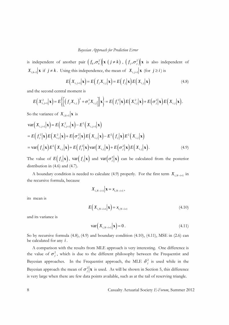
Bayesian Approach for Prediction Error
8 Casualty Actuarial Society E-Forum, Summer 2012
is independent of another pair 2,k kf x j k , 2,j jf x is also independent of
, 1i kX x if j k . Using this independence, the mean of , 1i jX x (for j i ) is
, 1 , ,i j j i j j i jE X E f X E f E X x x x x (4.8)
and the second central moment is
22 2, 1 , ,i j j i j j i jE X E f X X
x x 2 2 2
, ,j i j j i jE f E X E E X x x x x .
So the variance of , 1i kX x is
2 2, 1 , 1 , 1var i j i j i jX E X E X x x x
2 2 2 2 2, , ,j i j j i j j i jE f E X E E X E f E X x x x x x x
2 2 2, , ,var varj i j j i j j i jf E X E f X E E X x x x x x x . (4.9)
The value of jE f x , var jf x and 2var j x can be calculated from the posterior
distribution in (4.6) and (4.7).
A boundary condition is needed to calculate (4.9) properly. For the first term , 1i N iX in
the recursive formula, because
, 1 , 1i N i i N iX x x ,
its mean is
, 1 , 1i N i i N iE X x x (4.10)
and its variance is
, 1var 0i N iX x . (4.11)
So by recursive formula (4.8), (4.9) and boundary condition (4.10), (4.11), MSE in (2.6) can be calculated for any i .
A comparison with the results from MLE approach is very interesting. One difference is the value of 2
j , which is due to the different philosophy between the Frequentist and
Bayesian approaches. In the Frequentist approach, the MLE 2ˆ j is used while in the
Bayesian approach the mean of 2j x is used. As will be shown in Section 5, this difference
is very large when there are few data points available, such as at the tail of reserving triangle.

Bayesian Approach for Prediction Error
Casualty Actuarial Society E-Forum, Summer 2012 9
Another difference is that MSE of the Bayesian approach is larger than that of the Frequentist approach. Because the Frequentist approach always splits the total MSE into process error and parameter error, for comparison purposes, (4.9) is artificially split into a
process component and a parameter component, denoted as ,varpro i jX x and
,varpar i jX x , respectively. That is
, , ,var var vari j pro i j par i jX X X x x x (4.12)
Substitute (4.12) into (4.9) and (4.9) becomes
, 1 , 1var varpro i j par i jX X x x
2 2 2, , , ,var var varj i j j i j j pro i j par i jf E X E E X E f X X x x x x x x x .
(4.13)
If it is assumed that the process component follows the same recursive formula for the process risk as in the Frequentist approach [2], [10], then
, 1varpro i jX x 2 2, ,varj pro i j j i jE f X E E X x x x x . (4.14)
Substituting (4.14) into (4.13) gives the recursive formula for the parameter component
, 1varpar i jX x
2 2, , ,var var var varj i j j pro i j j par i jf E X f X E f X x x x x x x . (4.15)
The equivalent recursive formula for Mack’s formula [10] is
, 1varpar i jX x 2,var j i jf E X x x 2
,varj par i jE f X x x , (4.16)
which doesn’t have the term ,var varj i jf Xx x compared with (4.15). Murphy’s
formula [2], which is the recursive formula underlying BBMW’s formula [5], is
, 1varpar i jX x 2,var j i jf E X x x 2
,varj par i jE f X x x , (4.17)
which doesn’t have ,var varj pro i jf Xx x compared with (4.15). So the parameter error
component of the Bayesian approach is always larger than parameter error of the Frequentist approach. However, because this separation of process component and parameter component is artificial for the Bayesian approach, the only conclusion that can be made is that the total MSE of the Bayesian approach is larger than that of the Frequentist approach.

Bayesian Approach for Prediction Error
10 Casualty Actuarial Society E-Forum, Summer 2012
To calculate the variance of the aggregate claim amount in (2.7), a new sequence of random variables jZ are introduced to express the aggregate ultimate claim amount in
another way. jZ is defined as
1, ,2
N
j N j j i ji N j
Z x X
(4.18)
It is apparent that NZ is the aggregate ultimate claim amount. Based on (3.2), it is shown in Appendix A that
21 2, 3, , , 1, ,... ,j N j j N j j N j j j N j j j jZ X X X N f Z x Z . (4.19)
Then the total risk can be calculated in the same way as the individual year claims amount. For the boundary condition, 1 ,1NZ x , which is fixed, so the mean and variance of 1Z are
1 ,1NE Z xx
and
1var 0Z x ,
respectively. The recursive formula for mean of 1jZ is
1 , 1 , 1j j j N j j j j N j jE Z E f Z x E f E Z x x x x x (4.20)
and for variance is
2 21 1 1var j j jZ E Z E Z x x x
2 2 2 2 2j j j j j jE f E Z E E Z E f E Z x x x x x x
2 2 2var varj j j j j jf E Z E f Z E E Z x x x x x x , (4.21)
which is exactly same as the recursive formula for individual year.
5. PARAMETER ESTIMATION
As shown in last section, the posterior distributions for each pair of parameters 2,j jf
can be calculated individually and the posterior distributions in (4.5) have similar forms for different j ’s. To make the notation in further analysis more concise, the analysis in this section focuses on the term

Bayesian Approach for Prediction Error
Casualty Actuarial Society E-Forum, Summer 2012 11
2 22 2 22
1
1, exp ,
2
KK
i ii
p f x y f p f
x , (5.1)
with K replacing N j in (4.5). In this paper, f is always assumed unknown, while 2 could be known or unknown.
5.1 Known 2 For completeness and in order to make the comparison, this section includes a brief
analysis of the case when 2 is known, even though that was already been done in [8]. With known 2 , (5.1) is simplified to
2
21
1exp
2
K
i ii
p f x y f p f
x (5.2)
One typical non-informative prior distribution is
1p f . (5.3)
By substituting (5.3) into (5.2), there is
2
21
1exp
2
K
i ii
p f x y f
x
2
21
1 ˆexp2
K
ii
f f x
,
where
1 1
ˆK K
i i ii i
f x y x
. (5.4)
So the posterior distribution of f is a Normal distribution
2
1
ˆ ,K
ii
f N f x
x , (5.5)
and the mean is
ˆE f fx (5.6)
and the variance is
2
1
varK
ii
f x
x (5.7)

Bayesian Approach for Prediction Error
12 Casualty Actuarial Society E-Forum, Summer 2012
If there is prior knowledge of f , it is useful to use an informative prior distribution. One common option is the Normal distribution, i.e.,
2
02200
1exp
22
fp f
(5.8)
where 0 is the prior knowledge of f and 20 indicates the confidence about the prior
knowledge - a larger variance implying lower confidence. By this prior, the posterior distribution in (5.2) becomes
2 2
02 21 0
1 1exp
2 2
K
i ii
p f x y f f
x
2
02 2
1 02 2
1 02 2
1 0
ˆ
1 1exp
1 12 2
K
iKi
i Ki
ii
fx
x fx
which shows that posterior distribution is Normal distribution
02 2
1 0
2 2 2 21 10 0
ˆ
1,
1 1 1 1
K
iiK K
i ii i
fx
f Nx x
x .
5.2 Unknown 2
When the parameter 2 is unknown, there are usually three types of prior distributions depending on the philosophical view of the prior distribution.
5.2.1 Non-informative Prior
In a non-informative prior approach, the intention is to use a prior distribution as simple as possible, which provides the smallest amount of information. One option would be
2 2, 1p f . (5.9)
which is an improper prior distribution. Substitute this prior distribution into (5.1), the joint posterior distribution becomes
2 2 22 22
1
1, exp
2
KK
i ii
p f x x y f
(5.10)

Bayesian Approach for Prediction Error
Casualty Actuarial Society E-Forum, Summer 2012 13
As shown in Appendix B, the marginal posterior distribution f is
22
12
ˆ
11
KK
ii
f f xp f
K s
x , (5.11)
where f is defined in (5.4) and
22
1
1 ˆ1
K
i ii
s x y fK
, (5.12)
which is the MLE of variance 2 that is widely used in [1]-[8] for the Frequentist and semi-Bayesian approach. The distribution shown in (5.11) is the standard t -distribution [10] with
shift and scale, that is, 2
1
ˆK
ii
f f s x
has the standard t -distribution with
1K degrees of freedom. So the posterior distribution of f is the t -distribution
21
1
ˆ ,K
K ii
f t f s x
x . (5.13)
By feature of the t -distribution, the mean of f is
ˆE f fx (5.14)
and the variance is
2
1
1var
3
K
ii
Kf s x
K
x . (5.15)
So var f x is not defined for 3K .
Similarly, Appendix C shows the marginal distribution of 2 is
21 22 2
2
1exp
2
K K sp
x (5.16)
which indicates that 2 has inverse Gamma distribution with parameter 1 2K and
21 2K s , that is,
2 21 2, 1 2IG K K s x .
So the mean of 2 is

Bayesian Approach for Prediction Error
14 Casualty Actuarial Society E-Forum, Summer 2012
22 21 1
32 1 2 1
K s KE s
KK
x . (5.17)
Similar to var f x , this is not defined for 3K .
5.2.2 Conjugate Prior
In the conjugate prior approach, the philosophy is to choose a prior distribution that provides convenience of calculation. Typically the conjugate distribution will be used, that is the distribution which makes prior and posterior belong to same distribution family. For the likelihood formation as in (5.1), the conjugate distribution is the Normal-Inverse-Gamma distribution, which is defined as
2 2 2,p f p f p (5.18)
where 2 has inverse Gamma distribution
2 20 02, 2IG
and f has Normal distribution with variance related to 2
2 20 0,f N .
0 , 20 , 0 and 0 are all parameters that can be chosen based on prior knowledge. In
this prior distribution, f is no longer independent of 2 .
By these prior distributions, the posterior distribution (5.1) becomes
22 2 0 02 2
2 221
1 1, exp exp
2 22
KK
i ii
fp f x f y
x
02
2 12 02
exp2
0 3 2 2 22 20 0 02
1
1exp
2
KK
i ii
f x f y
. (5.19)
As shown in Appendix D, the marginal distribution of f is
1 22 2
1
K
K K K K
K
fp f
x (5.20)
where

Bayesian Approach for Prediction Error
Casualty Actuarial Society E-Forum, Summer 2012 15
0 10
0 01 1
ˆ
K
ii
K K K
i ii i
xf
x x
, (5.21)
01
K
K ii
x
, (5.22)
0K K , (5.23)
and 22 2 2 0
0 01
ˆ1K
K iiK
K s f x
. (5.24)
So 2K K K Kf has the standard t -distribution with K degrees of freedom,
that is
2,K K K K Kf t x ,
which gives the mean
KE f x (5.25)
and the variance
2 2
var2 2
K K K
K K K K K
f
x . (5.26)
Similarly, the marginal posterior distribution of 2 is
22 22 2
2exp
2K Kp
x (5.27)
which is proved in Appendix E. (5.27) shows that 2 has inverse Gamma distribution with parameter 2K and 2 2K , i.e.,
2 22, 2K KIG x .
So the mean is
2
2
2K
K
E
x . (5.28)

Bayesian Approach for Prediction Error
16 Casualty Actuarial Society E-Forum, Summer 2012
5.2.3 Other priors
The third option is to use any distribution that is ‘subjectively’ chosen based on prior knowledge. One commonly used prior distribution is that f and 2 are independent while
f has normal distribution and 2 has inverse Gamma distribution, that is,
2 2,p f p f p (5.29)
where
20 0,f N
and
2 20 02, 2IG .
This prior is quite similar to conjugate prior distribution in (5.18) but f and 2 are independent. Substitute this into (5.1), the joint posterior distribution is
22 2 02 2
2 221 00
1 1, exp exp
2 22
KK
i ii
fp f x f y
x
02
2 12 02
exp2
. (5.30)
So the marginal posterior distribution is
0
22 2 20 2 2 2
02 2010
1exp exp
2 2
KK
i ii
fp f x f y d
x
0
200
2 20 2 2
01
2exp
2 12
KK
i ii
Kf
x f y
02 2
20 202
10
exp2
KK
i ii
fx f y
,
which doesn’t follow any standard distribution but is still a closed-form distribution. The marginal distribution of 2 could be calculated in a similar way, but it does not give a closed-form result. However, the mean and variance of f and 2 can be calculated by numerical technique based on marginal posterior distribution. This approach is not developed further in this paper.

Bayesian Approach for Prediction Error
Casualty Actuarial Society E-Forum, Summer 2012 17
6. NUMERICAL EXAMPLE AND RESULTS
The data from Taylor and Ashe [12], which is in Table 1, is used to illustrate the analytical results from previous sections.
Table 1. Cumulative claims amount triangle.
i j 1 2 3 4 5 6 7 8 9 10
1
357,848
1,124,788
1,735,330
2,218,270
2,745,596
3,319,994
3,466,336
3,606,286
3,833,515
3,901,463
2
352,118
1,236,139
2,170,033
3,353,322
3,799,067
4,120,063
4,647,867
4,914,039
5,339,085
3
290,507
1,292,306
2,218,525
3,235,179
3,985,995
4,132,918
4,628,910
4,909,315
4
310,608
1,418,858
2,195,047
3,757,447
4,029,929
4,381,982
4,588,268
5
443,160
1,136,350
2,128,333
2,897,821
3,402,672
3,873,311
6
396,132
1,333,217
2,180,715
2,985,752
3,691,712
7
440,832
1,288,463
2,419,861
3,483,130
8
359,480
1,421,128
2,864,498
9
376,686
1,363,294
10
344,014
Four prior distributions are used; they are:
Prior 1: (5.3) with known variance 2 equaling 2s defined in (5.12). For the last variance of 2
9 , the formula does not work as there is only one observation of development factor, a
common issue in the Frequentist approach as well. The 29 is estimated according to
Mack’s suggestion in [1] as
2 4 2 2 29 8 7 7 8min ,min , ;
Prior 2: (5.9)
Prior 3: (5.18) with parameters 0 0 , 0 0.001 , 0 0.001 and 0 0.001
Prior 4: (5.18) with parameter 0 0 , 0 0.001 , 0 1.001 and 0 0.001
Prior 1 is the prior used by [3], [4], and [8] and served as benchmark in this example. Prior 2-4 are the priors where 2 is unknown. Prior 2 gives the least information about jf and 2
j ,
which is often called non-informative. Prior 3 is almost non-informative for 2j , but it does
give more information for jf compared with Prior 2 because the variance of jf could be

Bayesian Approach for Prediction Error
18 Casualty Actuarial Society E-Forum, Summer 2012
very small when 2j is small. Prior 4 has same implication for jf as Prior 3, and it gives
more information about 2j .
It is important to note that the chosen parameters uniquely define the prior distribution. However, that does not necessarily guarantee that statistical measures of the distribution, such as the mean and variance, exist. For example, for a non-informative prior, it is common to have infinite mean or variance.
First, the mean and variance of parameters jf and 2j are calculated. Equations (5.4),
(5.14), and (5.25) are used to calculate the mean of jf , shown in Table 2. As expected, the mean
is very similar among the different prior distributions.
Table 2. Results of jE f x
j Prior 1 Prior 2 Prior 3 Prior 4
1 3.4906065 3.4906065 3.4906055 3.4906055
2 1.7473326 1.7473326 1.7473325 1.7473325
3 1.4574128 1.4574128 1.4574127 1.4574127
4 1.1738517 1.1738517 1.1738516 1.1738516
5 1.1038235 1.1038235 1.1038235 1.1038235
6 1.0862694 1.0862694 1.0862693 1.0862693
7 1.0538744 1.0538744 1.0538743 1.0538743
8 1.0765552 1.0765552 1.0765551 1.0765551
9 1.0177247 1.0177247 1.0177245 1.0177245
The variance of jf is calculated using (5.7), (5.15) and (5.26), and is presented in Table 3.
In the tail of the triangle, the formula might not work--a similar issue when estimating 29 .
(5.15) and (5.26) do not work when the number of observation is small, which does not mean that the variance does not exist but that there is not enough information to estimate it under a non-informative prior. In such case, the approach suggested in [8] is used: the variance is estimated by multiplying the result of Prior 1 with a constant factor.
The multiplicative factor is chosen, subjectively, as the ratio of estimator of this Prior to
the estimator of Prior 1 at the nearest year where var jf x can be estimated. So for Prior
2, the factor is the ratio at year 6, which is 3. For Prior 3, it is the ratio at year 8, which is 2.
var jf x calculated by these factor are highlighted in Italic in the Table 3. Table 3 shows
that the differences in the variance between different prior distributions are quite large, while
Prior 4 gives very similar results to Prior 1 except that last term of 9var f x . This is

Bayesian Approach for Prediction Error
Casualty Actuarial Society E-Forum, Summer 2012 19
because at the extreme tail of triangle, the observed information is not enough to estimate the variance and the estimation largely depends on the prior information. As stronger prior is assumed in Prior 1, so the variance is lower.
Table 3. Results of var jf x .
j Prior 1 Prior 2 Prior 3 Prior 4
1 0.04817026 0.06422701 0.05504437 0.04816468
2 0.00368120 0.00515367 0.00429406 0.00368071
3 0.00278879 0.00418318 0.00334590 0.00278834
4 0.00082302 0.00137170 0.00102854 0.00082287
5 0.00076441 0.00152882 0.00101890 0.00076424
6 0.00051306 0.00153917 0.00076923 0.00051291
7 0.00003505 0.00010514 0.00007011 0.00003507
8 0.00013466 0.00040399 0.00026932 0.00013466
9 0.00011650 0.00034951 0.00023301 0.00027045
The mean of 2 is calculated using (5.17) and (5.28). For Prior 1, it is a fixed value given by (5.12). For Prior 2 and 3, if the formula does not work in the tail of triangle, the same
approach - multiplying results for Prior 1 by a factor - as for var jf x is used. All results
are shown in Table 4, which indicates the difference between prior distributions is also quite large.
Table 4. Results of 2jE x .
j Prior 1 Prior 2 Prior 3 Prior 4
1 160,280.327 213,707.103 183,153.093 160,261.818
2 37,736.855 52,831.597 44,019.503 37,731.901
3 41,965.213 62,947.820 50,348.611 41,958.574
4 15,182.903 25,304.838 18,974.230 15,180.142
5 13,731.324 27,462.648 18,302.737 13,728.197
6 8,185.772 24,557.315 1,2273.111 8,183.437
7 446.617 1,339.850 893.451 446.949
8 1,147.366 3,442.098 2,294.732 1,147.379
9 446.617 1,339.850 893.233 1,036.763
Then the MSE can be calculated. First, the recursive formulas by Mack (4.16) and BBMW/Murphy (4.17) are compared to the Bayesian approach (4.9) under Prior 1, with

Bayesian Approach for Prediction Error
20 Casualty Actuarial Society E-Forum, Summer 2012
results presented in Table 5. The results are exactly matched to results in [1], [3], [4] and [10], which shows that the Bayesian approach under Prior 1 is very similar to the Frequentist approach with a difference of 0.01% in reserve amount.
Table 5. MSE by Frequentist and Bayesian approaches under Prior 1.
Year Mack Murphy/BBMW Bayesian 2 75,535 75,535 75,535 3 121,699 121,700 121,703 4 133,549 133,551 133,556 5 261,406 261,412 261,436 6 411,010 411,028 411,111 7 558,317 558,356 558,544 8 875,328 875,430 875,921 9 971,258 971,385 972,234 10 1,363,155 1,363,385 1,365,456
Total 2,447,095 2,447,618 2,449,345 Total MSE in % 13.10% 13.10% 13.11%
Finally, the MSE under four different prior distributions are calculated in Table 6. The MSE under the non-informative prior distribution, i.e., Prior 2, is about 38% larger than that under Prior 1 or the MSE of the Frequentist approach, which shows that the MSE is greatly underestimated if the variance is assumed known or fixed.
The MSE is about a 3% different between Prior 1 and Prior 4 although the parameters estimated in Table 2-4 are very similar between these two prior distributions. This indicates that MSE is quite sensitive to parameters in the tail.
Table 6. MSE of different prior distributions.
Year Prior 1 Prior 2 Prior 3 Prior 4 2 75,535 130,831 106,823 115,086 3 121,703 210,810 172,120 149,104 4 133,556 231,348 188,890 158,383 5 261,436 452,921 332,284 273,259 6 411,111 641,245 495,957 419,342 7 558,544 816,905 655,425 565,685 8 875,921 1,184,204 995,294 882,037 9 972,234 1,259,424 1,085,789 976,334 10 1,365,456 1,664,613 1,488,920 1,367,860
Total 2,449,345 3,383,619 2,830,505 2,527,166 Total MSE in % 13.11% 18.11% 15.15% 13.53%

Bayesian Approach for Prediction Error
Casualty Actuarial Society E-Forum, Summer 2012 21
7. CONCLUSIONS
The general Bayesian approach to evaluate prediction uncertainty is first explained and compared with the Frequentist approach. The key difference is that the Bayesian approach evaluates the posterior distributions of unknown parameters, rather than point estimates as in the Frequentist approach. Due to this different philosophy, it has been shown that the total prediction uncertainty of the Bayesian approach is different from that of the Frequentist approach, and under certain assumptions the Bayesian approach gives a higher estimate.
In parameter estimation, the Bayesian approach also takes a different approach. Closed-form distributions for f and 2 are derived for several prior distributions in Mack’s model, which is one of the key results of this paper. It is shown that under non-informative and conjugate prior distribution, the posterior distribution of development factor f is the
standard t -distribution while 2 has inverse Gamma distribution. For some other prior distributions, it is possible to derive a closed-form distribution which doesn’t match any standard statistical distribution. It is also shown that if the parameter 2 is considered known and fixed, which is a very strong prior distribution assumption, the Bayesian approach gives the same result as the Frequentist approach. This indicates that the widely used Frequentist approach could underestimate the prediction uncertainty because it doesn’t full reflect the uncertainty of 2 .
The numerical results based on Taylor and Ashe data [12] are presented to confirm these conclusions. The Bayesian approach with strong prior distribution gives essentially the same results as Mack’s and Murphy/BBMW’s results. However, the prior distribution has a significant impact on the prediction uncertainty: a non-informative prior could increase aggregate prediction uncertainty by as much as 38%. Most of the difference comes from
var jf x and 2jE x . This highlights the problem of parameter estimations in chain
ladder method: with no prior knowledge, the estimation of development factor could be very volatile.
Acknowledgment
The author would like to thank reviewers Vladimir Shander and Nancy Arico for their comments and suggestions, which greatly improve readability of the paper. Appendix A. Proof of Equation (4.19)
It will be proved in recursive approach. By the assumptions of the model from (3.2), there is
21, 1 1,1 1, 1, 1,,..., ,N j N N j j N j j N jX X X N f X X
and 2, 1 ,1 , , ,,..., ,N j N N j j N j j N jX X X N f X X .

Bayesian Approach for Prediction Error
22 Casualty Actuarial Society E-Forum, Summer 2012
So the distribution of 1, 1 , 1 1,1 1, ,1 ,,..., , ,...,N j N j N N j N N jX X X X X X is
1, 1 , 1 1,1 1, ,1 ,,..., , ,...,N j N j N N j N N jp X X x X X X X
1, 1 1,1 1, , 1 ,1 ,,..., ,...,N j N N j N j N N jp X t X X p X x t X X dt
2 2
1, ,
2 22 21, ,1, ,
1 1exp exp
2 22 2
j N j j N j
j N j j N jj N j j N j
t f X x t f Xdt
X XX X
2
1, ,
221, ,1, ,
1exp
22
j N j N j
j N j N jj N j N j
x f X X
X XX X
,
which shows that it is Normal distributed with mean 1, ,j N j N jf X X and variance
21, ,j N j N jX X . Recursively, 2, 1N jX , 3, 1N jX ,…, 1, 1N j jX can be put into
summation and the sum , 11
N
i ji N j
X is Normal distribution with mean ,
1
N
j i ji N j
f X and
variance 2,
1
N
j i ji N j
X . So by the definition of 1jZ in (4.18), there is
21 , 1 , 1 , , 1 ,
1 1 1
,N N N
j N j j i j j i j N j j j i ji N j i N j i N j
Z x X N f X x X
2, 1,j j N j j j jN f Z x Z .
Appendix B. Proof of Equation (5.11)
By substituting (5.10) into (4.6), the posterior distribution of f is
2 2 22 220
1
1exp
2
KK
i ii
p f x y f d
x
2
2
1
2
12
KK
i ii
K
x y f
2
2
1
KK
i ii
x y f

Bayesian Approach for Prediction Error
Casualty Actuarial Society E-Forum, Summer 2012 23
2
2 2
1 1
ˆ ˆKK K
i i ii i
x f f x y f
22
12
ˆ
11
KK
ii
f f x
K s
.
Appendix C. Proof of Equation (5.16)
By substituting (5.10) into (4.7), the posterior distribution is
2 2 22 22
1
1exp
2
KK
i ii
p x y f df
x
2 22 222 2
1 1
1 1ˆ ˆexp exp2 2
K KK
i i ii i
x y f x f f df
22 22 22
1 1
1 ˆexp 22
K KK
i i ii i
x y f x
21 22
2
1exp
2
K K s
.
Appendix D. Proof of Equation (5.20)
Substituting (5.19) into (4.6), there is
0 3 2 2 22 2 20 0 020
1
1exp
2
KK
i ii
p f f x f y d
x
0
0
1 22 2 2
0 0 01
1 2
12
KK
i ii
K
f x f y
0 1 2
2 2 20 0 0
1
KK
i ii
f x f y
0 1 2
2 22 20 0 0
1 1
ˆ ˆKK K
i i ii i
f x f f x y f

Bayesian Approach for Prediction Error
24 Casualty Actuarial Society E-Forum, Summer 2012
0 1 2
22 2 2 2
0 0 0 0 0 01 1 1 1
ˆ ˆ ˆ2K
K K K K
i i i i ii i i i
x f f x f f x x y f
0 1 222
0 0 0 0 21 21
0 01 1
0 01 1
ˆ ˆˆ
KK K
i iK Ki i
i i iK Ki i
i ii i
f x f xx f x y f
x x
1 22
0 02 2 21
0
ˆ
1
KK
ii
K KK
f xf K s
1 22 2
1
K
K K K K
K
f
where K , K , K and 2K are defined in (5.21)-(5.24).
Appendix E. Proof of Equation (5.27)
Substitute (5.19) into (4.7), the posterior distribution of 2 is
0 1 2 1 2 22 2 20 0 02
1
1exp
2
KK
i ii
p f x f y df
x
2 21 2 22 20 0 02
1 1
1 ˆ ˆexp2
KK K
i i ii i
f x f f x f y df
1 2 22 22
1exp
2K
K K Kf df
221 22
2
2exp
2K K
K
22 22
2exp
2K K
.

Bayesian Approach for Prediction Error
Casualty Actuarial Society E-Forum, Summer 2012 25
REFERENCES
[1] Mack T., “Distribution-free calculation of the standard error of chain-ladder reserve estimates,” ASTIN Bulletin, 23(2), 213-225.
[2] Murphy D. M., “Unbiased loss development factors,” PCAS 81, 154-222. [3] England P. D. and Verrall R. J., “Stochastic claims reserving in general insurance,” British Actuarial Journal, 8,
443-544. [4] England P. D. and Verrall R. J., “Predictive distributions of outstanding liabilities in general insurance,”
Annual of Actuarial Study, 1, 221-270. [5] Buchwalder M., Buhlmann H., Herz M., and Wuthrich M. V., “The mean square error of prediction in the
chain ladder reserving method”, ASTIN Bulletin, 36(2), 521-542. [6] Mack T., Quarg G., and Braun C., “The mean square error of prediction in the chain ladder reserving
method – a comment,” ASTIN Bulletin, 36(2), 543-552. [7] Venter G., “Discussion of mean square error of prediction in the chain-ladder reserving method,” ASTIN
Bulletin, 36(2), 566-572. [8] Gisler A., “The estimation error in the chain-ladder reserving method: a Bayesian approach,” ASTIN
Bulletin, 36(2), 554-565. [9] Scollnik D. P. M., “Bayesian reserving models inspired by chain ladder methods and implemented using
WinBUGS,” [10] Murphy D. M., “Chain ladder reserve risk estimators,” CAS E-Forum Summer, 2007. [11] Patel J. K., Kapadia C. H., and Owen D.B., “Handbook of statistical distributions,” Marcel Dekker, Inc, 1976. [12] Taylor G. and Ashe G., “Second moments of estimates of outstanding claims,” Journal of Econometrics, 23,
37-61. [13] Bayarri M. J. and Berger J. O., “The Interplay of Bayesian and Frequentist Analysis,” Statistical Science Vol. 19, No. 1 (Feb., 2004), pp. 58-80. Biography of the Author
Dr. Ji Yao is a manager of European Actuarial Services at Ernst & Young LLP. Since he graduated with a PhD in mathematics and statistics in 2005, he mainly practices in general insurance and specializes in statistical modeling and pricing. He qualified as a Fellow of Institute of Actuaries in 2008. He has also participated in various research projects, including reserving and Solvency II, and is a frequent speaker at international actuarial conferences.

1
Sustainability of Earnings: A Framework for Quantitative Modeling of Strategy, Risk, and Value
Neil M. Bodoff, FCAS, MAAA ________________________________________________________________________ Abstract
The value of a firm derives from its future cash flows, adjusted for risk, and discounted to present value. Much of the existing literature addresses the quantitative techniques for calculating probability distributions of future cash flows, calculating values of risk adjustment factors, and calculating values of discount factors. Yet strategy and strategic risk – for example, the risk of adverse consequences arising from the actions of new competitors, governmental intervention, customer changes, etc. – often cannot easily be incorporated into this quantitative framework. As a result, strategic concerns are addressed in a parallel track of qualitative analysis, which supplements the quantitative analysis but never integrates with it. The goal of this paper is to propose in detail a quantitative framework in which strategic considerations can be incorporated into a quantitative model of the value of the firm. The resulting framework seeks to measure not only the amount, growth rate, and variability of earnings, but also the firm’s “sustainability of earnings” and value in the face of strategic forces. Keywords. Strategy, Risk, Value, ERM, Sustainability of Earnings.
1. INTRODUCTION
Strategy is a source of risk to the firm and thus ought to be included within enterprise risk management (ERM), enterprise risk analysis, and measurement of the firm’s value. Yet while detailed quantitative models describe other sources of risk such as financial risk, operational risk, and hazard risk, the quantitative apparatus for incorporating strategy into a model of the firm is often underdeveloped or simply lacking. As a result, analysts address strategic forces in a parallel track of qualitative analysis, which supplements the quantitative analysis but cannot integrate with it.
This paper proposes a detailed framework in which strategic considerations can be incorporated into a quantitative model of the firm. Such a framework incorporates a scenario-based paradigm, which allows one to develop a range of future strategic conditions; one must estimate the likelihood of such conditions materializing and what the ramifications would be for the firm’s earnings. This framework thus requires one to reflect upon and estimate the relative vulnerability of the firm’s earnings to changes in the strategic landscape; or, equivalently, the invulnerability or “sustainability” of the firm’s earnings with respect to strategic forces. By incorporating strategic forces into the quantitative risk model, one captures a broader range of variability in future earnings. Such a model could be used for measuring risk and volatility in a classic risk modeling framework; further, following the

Sustainability of Earnings: A Framework for Quantitative Modeling of Strategy, Risk, and Value
2
paradigm of Panning [4], one can use such a framework to calculate the value of a business based on its future earnings. This has particular application to the problem of estimating the relative value of two businesses with differing degrees of earnings sustainability in the face of strategic forces. It also provides a pathway towards quantifying a cost-benefit evaluation of expenditures on strategic maneuvers designed to enhance the firm’s strategic posture.
1.1 Research Context
Slywotzky and Drzik [7] address strategy and strategic risk, but their focus is on deploying countermeasures to strategic risk. Their treatment is mostly qualitative; although they state the importance of estimating the likelihood and severity of various strategic risks, this recommendation leads only to a risk map that does not integrate into an overall quantitative risk model of the firm. Mango [3] provides a general introduction to strategic risk issues, with a focus on scenario planning and risk modeling; he notes the lack of precision in the terms “strategy” and “strategic risk”. Schelling [6] serves as our starting point for how strategy is defined in this paper, leading to the crystallization by Porter [5]. We incorporate our risk model of strategy into the framework for the value of the firm developed by Panning [4], who was not addressing strategy per se but rather the risk of downside financial variability; the framework nevertheless is suitable for our purposes. Finally, we note that an antecedent to the proposed model can be found in Feldblum [2], who proposed the approach at a more granular policy level rather than at the business unit or firm level.
1.2 Objective
The objective of this paper is to describe a practical framework that can incorporate the quantitative modeling of risks emanating from a firm’s strategic position.
2. STRATEGY
2.1 Schelling and the Theory of Games
In this paper, we will use as a starting point the description presented by Schelling [6]. He notes that in the field of Game Theory, a game of strategy refers to:
“[a situation] in which the best course of action for each player depends on what the other players do. The term is intended to focus on the interdependence of the

Sustainability of Earnings: A Framework for Quantitative Modeling of Strategy, Risk, and Value
3
adversaries’ decisions and on their expectation about each other’s behavior”.
Schelling directs our attention to how the firm’s results can be affected by other players whose rational actions interact with and impact upon the firm. This point is crucial because so much of current practice in the property-casualty insurance industry focuses on modeling the variability of a firm’s financial results based on fortuitous events, for example property damage claims from natural catastrophes or liability claims from car crashes. Thus Schelling’s definition of strategy, focusing on the actions of competing players, leads us to consider a category of risk that is not currently encapsulated in other risk categories such as operational risk, hazard risk, or financial risk.
2.2 Buffet’s Economic Moat and Porter’s Five Forces
Our focus on the actions of other players leads us to consider competition and competitive forces. How do competitive forces potentially affect the firm? One vivid metaphor, articulated by Warren Buffet, is the “economic moat”. The idea behind this metaphor is to consider the relative safety or vulnerability of a business’s earnings and value in the face of competitive forces.
In order to gain greater insight into competitive forces, we invoke the classification system devised by Porter [5]. To describe competition, he details the Five Forces that govern the competitive landscape:
1. Threat of new entrants
2. Jockeying for position among current competitors
3. Bargaining power of suppliers
4. Bargaining power of customers
5. Threat of substitute products
6. [Threat of government intervention]
2.3 Sustainability of Earnings
Porter’s classification accentuates that a firm’s current earnings and value are potentially vulnerable to the competitive forces of suppliers, customers, and new competitors. Thus in evaluating a business, one must consider not only the amount of the business’s earnings and

Sustainability of Earnings: A Framework for Quantitative Modeling of Strategy, Risk, and Value
4
the growth rate of its earnings, but also its “sustainability of earnings”.
We define “sustainability of earnings” as the likelihood that a business’s earnings will not be eroded by the strategic moves of competitive forces.
Sustainability of earnings provides a framework for evaluating the value of a firm, the price of an acquisition, and the value of a business unit or product line within a conglomerate.
For example, in the property-casualty insurance industry, one can ask of each line of business:
1. Threat of new entrants:
a. What kind of barriers to entry does this line of business have?
i. To what extent does it require hard to obtain, specialized, technical underwriting skills?
ii. To what extent does it require access to distribution channels?
iii. To what extent does obtaining business require a proven track record of claims paying and reliability?
2. Bargaining power of suppliers:
a. To what extent do the suppliers of capital have pricing power and availability power over this business?
i. To what extent does writing this line of business require the support of suppliers of reinsurance capital?
ii. Could the business easily switch to alternative forms of capital, including capital markets instruments such as cat bonds, or, alternatively, rely on the firm’s held equity capital?
3. Bargaining power of customers:
a. To what extent do customers have the ability to change their purchasing behavior?
i. Do they have the ability and willingness to choose not to purchase the insurance product that the firm offers and simply

Sustainability of Earnings: A Framework for Quantitative Modeling of Strategy, Risk, and Value
5
retain the risk for themselves?
All of these questions are relevant whenever:
1. A conglomerate’s senior management is measuring the value of various subsidiaries or lines of business in its portfolio of products and businesses.
2. A company is estimating how much to pay to acquire another company or to pay for new talent to develop a new line of business.
3. Senior management is evaluating strategic moves to enhance the value of the firm and thus to increase its stock price.
3. MODELING
One might desire to describe strategy and competitive forces via a quantitative or even a probabilistic model, especially a probabilistic model that incorporates other sources of risk to the firm, such as financial risk and hazard risk. How might one go about doing so? By focusing on sustainability of earnings, we can begin to develop such a framework.
3.1 Modeling the Risk to the Firm: Single Period Variability of Earnings
We can model any of the competitive forces described by Porter as a random variable. As an example, let’s focus on one particular competitive force: the threat of new entrants.
Let X be a random variable with a Bernoulli probability distribution:
Probability Outcome State Description
p 1 success No new competitor enters the business
1-p 0 failure A significant new competitor enters the business
In order to implement such a model, one would need to estimate the probability of a new competitor entering the business. Some examples of how to estimate this probability, including using expert opinion, can be found in Appendix B of the monograph “Overview of Enterprise Risk Management” [1].
In addition to estimating the probability of a new competitor entering the business, one

Sustainability of Earnings: A Framework for Quantitative Modeling of Strategy, Risk, and Value
6
should also evaluate the severity of such an event on business’s amount of earnings, as noted by Slywotzky and Drzik [7]. In the context of a full probability distribution model of earnings, a new competitor could affect not only the firm’s mean level of earnings but also the shape, volatility, and downside of its earnings.
Thus one could stipulate as follows:
Probability Description Ramification
P No new competitor enters the business
Company earnings follow distribution function F1(x)
1-p A significant new competitor enters the business
Company earnings follow distribution function F2(x)
For example:
1. Simulate a uniform distribution on [0,1]
a. If simulated output is on the interval [0,p] then you have a “success”, no new competitor has entered.
i. Simulate the business’s earnings via probability distribution #1.
b. If simulated output is on the interval (p,1] then you have a “failure”, a significant new competitor has entered the business.
i. Simulate the business’s earnings via probability distribution #2.

Sustainability of Earnings: A Framework for Quantitative Modeling of Strategy, Risk, and Value
7
Exhibit 1
0.000%
0.100%
0.200%
0.300%
0.400%
0.500%
0.600%
‐200 ‐170 ‐140 ‐110 ‐80 ‐50 ‐20 10 40 70 100 130 160 190
Prob
ability
Earnings
Probability Density Function of Company Earnings #1: No New Entrant
Probability Density Function of Company Earnings #2: Significant New Entrant
While this example deals with the probability of a significant new competitor entering the business, a similar approach can be used for the other forces, such as the probability of a major shift in pricing by suppliers or a major shift in purchasing behavior by customers.
3.2 Modeling the Value of the Firm
Until now we have focused on the sustainability of earnings in one future period, which accentuates the range of outcomes for the firm. How can measuring the sustainability of earnings translate into measuring value?
Here we invoke the framework developed both by Feldblum [2] and Panning [4], albeit in modestly different contexts. Feldblum addresses customer persistency, the probability that a particular customer will continue to purchase the insurance product, in evaluating the profitability of various types of customer segments and insurance contracts. Panning addresses the larger question of the value of the firm; he focuses on the probability of the

Sustainability of Earnings: A Framework for Quantitative Modeling of Strategy, Risk, and Value
8
firm having sufficient capital to survive its own downside financial events. Here we will deploy the same approach in order to measure the value of the firm in the face of a competitive force such as a potential new entrant to the business.
Following Panning’s model, we set the value of the firm equal to the present value of its future expected earnings:
Let:
E = expected earnings at time 1
DF = 1 / (1+r) = earnings discount factor
Value = ∑ E * DFt
Value = E * DF/(1-DF) = E * (1/r)
Now let’s introduce an earnings growth factor:
GF = (1+g)
Value = ∑ E * GFt-1 * DFt
Value = E * DF/(1-GF * DF) = E * (1/(r-g))
These equations for value mimic the standard results in financial textbooks. They incorporate earnings, discounting, and growth.
Now let’s introduce strategic concerns and sustainability of earnings in the face of competitive forces.
Let:
• p = annual probability of “success” = no significant new competitor enters the business in a given year.
• 1-p = annual probability of “failure” = a significant new competitor enters the business in a given year
We’ll also make two simplifying assumptions:
1. The company’s earnings become zero when a significant new competitor enters the business
2. Once a new competitor enters the business, no competitors drop out, and the

Sustainability of Earnings: A Framework for Quantitative Modeling of Strategy, Risk, and Value
9
company’s earnings prospects remain thereafter at zero.
Now we can say that in order for the company to realize earnings at time t, it must have a string of strategic “successes” such that no significant new competitor has entered the field.
Therefore:
Et = pt * E * GFt-1 + (1-pt) * 0 = pt * E * GFt-1
Then:
Value = ∑ E * pt * DFt * GFt-1
Value = E * p * DF / (1 – GF * p * DF)
Therefore, when p, the “sustainability of earnings” against competitive forces, is higher, the value of the business under consideration is higher.
Exhibit 2 shows a simplified numerical example of two hypothetical businesses. Firm A has higher earnings than Firm B, but Firm B has a forecast higher likelihood of sustaining its earnings in the face of competitive threats. Therefore, Firm B has a higher value; Firm A’s higher earnings are offset by a lower Price-to Earnings (P/E) multiple, while Firm B’s wider “economic moat” is reflected in its higher P/E multiple. Thus deploying Panning’s model allows one to estimate, within a quantitative model of the firm’s value, how much a firm’s strategic position is worth.

Sustainability of Earnings: A Framework for Quantitative Modeling of Strategy, Risk, and Value
10
Exhibit 2
Firm A Firm B(1) E = expected earnings 100.0 90.0(2) r 10.0% 10.0%(3) DF = 1/(1+r) 90.9% 90.9%(4) g = growth rate 5.0% 5.0%(5) GF = 1+g 1.05 1.05 (6) p 96.0% 98.0%(7) 1-p 4.0% 2.0%(8) Value 1043.5 1242.3(9) P/E multiple 10.4 13.8
Notes(8) = (1) * { (6) * (3) } / {1 - (5) * (6) * (3) }(9) = (8) / (1)
3.3 Modeling the Value of Strategic Maneuvers
We can use the model of the value of the firm not only to compare two different businesses, but also for a given firm to evaluate two alternative strategic moves.
Let’s say a firm is considering whether or not to increase its expenditures on initiatives that will increase the sustainability of earnings. For example, it might be considering increasing expenditures on advertising to enhance brand name recognition. Or it might be thinking about increasing research and development expenditures; the product enhancements from the additional R&D are not foreseen as increasing the firm’s earnings, but rather the enhanced product offering could serve as a barrier to entry to potential competitors. Or the firm might be contemplating spending more money on customer loyalty programs.
In all of these instances, the firm ought to forecast whether the benefit of the plan exceeds the cost. While ultimately there would be several different perspectives influencing the final decision, one would ideally like to be able to contribute a quantitative analysis as one component of the decision making process.
First we would need a basic description of the key aspects of the firm in its current state.
Sustainability of Earnings: A Framework for Quantitative Modeling of Strategy, Risk, and Value
11
We’ll start with the same information for Firm A as in Exhibit 2: we assume the firm has earnings of 100 and an annual probability p of sustainability of 96%, i.e. (1-p) probability of 4% that a new competitor will enter the business and decimate the firm’s earnings. Now the firm is considering how much (if any) additional expenditures it should make to strengthen its strategic position and reduce the likelihood of a new entrant to the market. Since the firm is currently spending some money on these activities and its probability p of sustainability is 96%, we assume that the additional expenditures will increase this probability from 96% at a minimum towards a maximum of 100%.
Let’s estimate a function that will help describe this relationship:
p = initial probability of sustainability
1-p = complement of p; maximum amount of improvement in p
x = additional new expenditures (as a % of current earnings) to enhance sustainability
f(x) = additive amount of percentage points of improvement in p = (1-p) * x / (x + k)
k = estimated parameter; for example, 10%
g(x) = improved probability p of sustainability = p + f(x) = p + (1-p) * x / (x + k)
In our example:
p = 96%
1-p = 4%
k = 10%
Then:
f(x) = 4% * x / (x + 10%)
g(x) = 96% + 4% * x / (x + 10%)

Sustainability of Earnings: A Framework for Quantitative Modeling of Strategy, Risk, and Value
12
Exhibit 3
0.00%
0.50%
1.00%
1.50%
2.00%
2.50%
3.00%
3.50%
4.00%0% 4% 8% 13%
17%
21%
25%
29%
34%
38%
42%
46%
50%
55%
59%
63%
67%
71%
76%
80%
84%
88%
92%
97%
Additional Expenditure as % of Earnings
f(x) = Additive Increase in Sustainability
Exhibit 4
94.00%
95.00%
96.00%
97.00%
98.00%
99.00%
100.00%
0% 4% 8% 13%
17%
21%
25%
29%
34%
38%
42%
46%
50%
55%
59%
63%
67%
71%
76%
80%
84%
88%
92%
97%
Additional Expenditure as % of Earnings
g(x) = Improved Value of Sustainability Parameter p
Now recall from Section 3.2 that the formula for the value of the firm depends upon earnings, growth, discount factor, and probability p of sustainability:

Sustainability of Earnings: A Framework for Quantitative Modeling of Strategy, Risk, and Value
13
Value = E * p * DF / (1 – GF * p * DF)
Therefore, each choice of additional expenditure will generate not only a revised amount of earnings and a revised parameter p, but also a revised quantity for the value of the firm:
Exhibit 5
‐
200.00
400.00
600.00
800.00
1,000.00
1,200.00
1,400.00
0% 4% 9% 13%
18%
22%
26%
31%
35%
40%
44%
48%
53%
57%
62%
66%
70%
75%
79%
84%
88%
92%
97%
Additional Expenditure as % of Earnings
Value of the Firm
Exhibit 5 highlights that in this numerical example, choosing to increase expenditures on strategic moves would increase the value of the firm, so long as the expenditure does not consume too much of the firm’s earnings. At some tipping point, however, one reaches a level such that further increases in expenditure actually reduce the value of the firm. This decrease in value occurs because the additional enhancement to sustainability is more than offset by the reduction in earnings. Yet for small and medium sized increases in expenditures, the value of the firm increases. The analysis framework allows one to calculate the optimal amount to invest in new strategic maneuvers in order to maximize the value of the firm.
4. CONCLUSIONS
A firm ought to be concerned about strategy and competitive forces. It should therefore integrate strategy considerations both when measuring holistically the firm’s total risk as well

Sustainability of Earnings: A Framework for Quantitative Modeling of Strategy, Risk, and Value
14
as when seeking to maximize the firm’s total value. In order to do so, we introduce the framework of “sustainability of earnings”; the various strategic forces that are described qualitatively in the strategy literature can thus be quantified as sources of risk whose outcomes can be described via probabilistic models. Such an approach allows one to incorporate strategic forces into the existing framework of probabilistic enterprise risk models. It also allows one to incorporate strategic considerations when calculating the value of a business, when comparing the relative attractiveness of two different businesses, and when calculating the benefits of various strategic maneuvers.
5. REFERENCES
[1] CAS Enterprise Risk Management Committee, “An Overview of Enterprise Risk Management”, 2003, http://www.casact.org/research/erm/overview.pdf
[2] Feldblum, Sholom, “Personal Automobile Premiums: An Asset Share Pricing Approach for Property/Casualty Insurance”, Proceedings of the CAS, 1996, Vol. LXXXIII, Part 2, 190-296, http://www.casact.org/pubs/proceed/proceed96/96190.pdf
[3] Mango, Donald, “An Introduction to Insurer Strategic Risk”, ASTIN Colloquium, 2005, http://www.actuaries.org/ASTIN/Colloquia/Orlando/Papers/Mango1.pdf
[4] Panning, William H., “Managing the Invisible: Measuring Risk, Managing Capital, Maximizing Value”, 2006 ERM Symposium, http://www.ermsymposium.org/2006/pdf/papers/Panning%204-10-06.pdf
[5] Porter, Michael E., “How Competitive Forces Shape Strategy”, Harvard Business Review, 1979 [6] Schelling, Thomas C., The Strategy of Conflict, 1980 [7] Slywotzky, Adrian J., and John Drzik, “Countering the Biggest Risk of All”, Harvard Business Review, 2005
Please send correspondence to [email protected] and [email protected].

Casualty Actuarial Society E-Forum, Summer 2012 1
A Common Subtle Error: Using Maximum Likelihood Tests to Choose between
Different Distributions
By Gyasi Dapaa1
Predictive Modeling Group, Allstate Insurance, Northbrook, IL
The Maximum Likelihood Estimation (MLE) is one of the most popular methodologies used to fit a parametric distribution to an observed set of data. MLE’s popularity stems from its desirable asymptotic properties. Maximum Likelihood (ML) estimators are consistent, which means that as the sample size increases the researcher becomes increasingly confident of obtaining an estimate that is sufficiently closer to the true value of the parameter; they are asymptotically normal with the lowest possible variance (achieve the Cramer-Rao lower bound on variance), which makes inference tests relatively easy and statistically more powerful. In addition, they are translation-invariant, which means that all functions of the ML estimates are by default the MLE predictors of the respective functions. For instance, if a pricing analyst computes pure premium from relativities estimated by MLE, the predicted pure premium is also an ML estimate and, hence, satisfies all the desirable aforementioned properties. Because of the known asymptotic distribution of ML estimators, there are numerous asymptotic tests to help researchers make statistical inferences about their ML estimates: examples include, among others, the Likelihood Ratio Test, the Lagrange Multiplier Test, and the Schwarz Bayesian Criterion (SBC). In general, all of these aforementioned tests are used to determine if the measured signals (the ML estimates) are statistically different from some pre-specified values. For instance, suppose a researcher believes that frequency follows a Poisson distribution with mean λ, and computes the sample mean as the MLE for λ. To test whether or not the measured signal is noise, the researcher may use one of these tests to check whether the ML estimate is statistically different from zero. In addition, the researcher may use one of these tests to check whether the ML estimate(s) is (are) statistically different from some pre-conceived or historic values. However, the aforementioned tests may not be used to make inferences about the functional form of the distribution of the data. In other words, as an example, one may not compare the ML values (as is implicitly done by these tests) to choose between a Poisson and a Negative Binomial distribution. This article argues why such a comparison is incorrect and would be no better than an apple to orange comparison. A critical assumption underlying MLE is that the researcher knows everything but a finite number of parameters of the specified distribution. (The functional form of a distribution has an infinite dimension). An implication of this is that this estimation technique could only be used after the functional form of the distribution (hence forth, simply referred to as the distribution) has been pre-specified. That is, a researcher needs to first specify whether the data is Poisson, Negative Binomial, Exponential, Lognormal, etc. before she could use the MLE technique to estimate the unknown parameters of the pre-specified distribution. Hence, the reader should easily see that the
1 The author holds a Master’s degree in Economics with a concentration in Econometrics and is currently an actuarial candidate.

A Common Subtle Error: Using Maximum Likelihood Tests to Choose between Different Distributions
Casualty Actuarial Society E-Forum, Summer 2012 2
MLE technique doesn't have the capability to determine the distribution of an observed data; otherwise, such a pre-specification of distribution would be unnecessary. There is even a subtle contradiction invoked by comparing ML values obtained under different distribution assumptions as these tests implicitly do. For instance, if we assume data follows a Normal distribution and hence use the sample mean as the MLE of the shape parameter, it is easy to see that the sample mean would no longer be an MLE upon discovery that our data actually follows a Pareto distribution. In other words, since a given data could only follow one distribution and since the ML estimator is valid only when the assumed distribution is right, comparing MLEs obtained under different distributions is self-contradictory! The reader should note, however, that distributions with different names do not necessarily have different functional forms. For instance, the Exponential and the Gamma distributions have the same functional form but differ only in the value of the shape parameter. (In other words, they differ in a finite number of parameters.) In fact, the Exponential distribution is a special form of the Gamma distribution. Hence, the ML tests are valid and can be used to make inferences about whether or not the shape parameter is one (and hence Exponential). However, when the two distributions are rather distinct in functional form, but not in parameter values (such as the Weibull and Lognormal distributions), the ML tests are invalid!2
In light of the above argument, all MLE inference tests such as the Likelihood Ratio Test, the Lagrange Multiplier Test, and the Schwarz Bayesian Criterion (SBC) are not appropriate under different distributions. Unfortunately, many researchers unknowingly misapply these tests to choose between distributions, e.g., Poisson vs. Negative Binomial). Even in much of the exam oriented actuarial literature such as Manuals for Actuarial Exam 4/C, as well as some past exams, have questions that mistakenly ask candidates to use one of these ML tests to make inferences about different distributions. It is also worthy to point out that, under such scenarios, the inference statistics such as the Likelihood Ratio Statistic and the SBC are not only meaningless, but do not even follow a Chi-square distribution (as they traditionally do); hence, using the Chi-square critical regions to accept or reject the null hypothesis is erroneous. An important question, therefore, is what tests can a researcher use to choose between different distributions. There are numerous statistical tests of distribution fit: Kolmogorov-Smirnov tests and Chi-square Goodness of Fit tests are examples of such tests. These tests tell the modeler whether or not there is good reason to trust the fitted distribution. Unfortunately, each of these tests could accept multiple distributions as good fits. When this happens, the modeler could choose the distribution with the maximum3
2 There is, however, a hot debate about the validity of MLE when functional forms are parameterized so that they differ by a finite number of parameters. For instance, the Tweedie distribution could be parameterized by a p-parameter so that, by changing the p-parameter, the assumed functional form of the distribution changes.
p-value.
3 Notice that for most inference tests about distributions, a high p-value is support for the null hypothesis (the distribution being tested).

Loyalty Rewards and Gift Card Programs: Basic Actuarial Estimation Techniques
Tim A. Gault, ACAS, MAAA, Len Llaguno, FCAS, MAAA and
Martin Ménard, FCAS, MAAA ___________________________________________________________________ Abstract
In this paper we establish an actuarial framework for loyalty rewards and gift card programs. Specifically, we present models to estimate redemption and breakage rates as well as to estimate cost and value for use in both accrued cost and deferred revenue accounting methodologies. In addition, we provide guidance on various issues and considerations that may be required of an analyst when working with loyalty rewards and gift card programs.
Keywords: loyalty rewards, gift cards, redemption rate, breakage, liability estimation, cost estimation, accrued costs, deferred revenue
1. INTRODUCTION
The size and scope of loyalty reward programs has grown immensely over the last several
decades. Since the rise of airline frequent flyer programs in the 1980s, loyalty programs in
their modern form have become deeply intertwined within corporate marketing strategies.
From the financial services industry with its rewards-based credit cards, to the hospitality
services industry with hotel reward programs, to gift cards and other coupons issued by
common brick and mortar industries such as food services and clothing retailers, to the
frequent flyer airline miles programs, reward programs can now be found almost
everywhere. While rewarding frequent customers with perks, benefits, discounts or
complimentary product has been a long-standing business practice in marketing spheres, it
has become ever more important to other areas of business practices within companies. In
fact, member loyalty and gift card programs have moved into upper managements’
companywide purview as a core component of brand strategies and are furthermore now
often an integral part of corporate identities themselves. The elevation of importance now
requires practitioners to stretch across the sometimes siloed practices of marketing, finance,
accounting, and information technology departments within a company.
Reward programs essentially consist of promises made today to deliver something
tomorrow, or next year, or potentially never. The nature of reward programs often brings
with it significant challenges. Many reward programs’ structures are built around uncertain
Casualty Actuarial Society E-Forum, Summer 2012 1

Loyalty Rewards and Gift Card Programs: Basic Actuarial Estimation Techniques
future events: contingencies of “how much,” “when,” and “if.” Additionally, a program’s
terms and conditions can change as the program evolves, leading to material changes to the
benefits that participating members can obtain, or to the costs that sponsors will encounter.
These uncertainties often obfuscate the value or costs that a sponsor is promising.
Furthermore, these uncertainties can often challenge one’s ability to estimate the future
benefits and costs of a program in an accurate and substantive way.
Fortunately, the amount of information collected and available to program providers
presents an exceptional opportunity to truly understand the costs and revenue drivers of
their programs and to measure them in an accurate and timely manner. This large amount of
information can be used to design programs that provide better “rewards” to their members,
maximize the value of the program to its sponsor by generating incremental revenue due to
increased members’ loyalty, and help in providing quantified feedback to management and
other financially interested players.
It is our hope that the tools presented in this paper can provide guidance to an analyst
(and an actuary!) as to how to think about some of the economic fundamentals of loyalty
rewards and gift cards programs, and to place a more structured quantitative framework
around understanding and measuring their impact on the companies that offer them.
2. OVERVIEW OF REWARD PROGRAMS
2.1 Program Basics
The basic premise of reward programs consists of “members” purchasing goods or
services in exchange for a promise, by the reward program sponsor, to provide additional
future goods, services, or value to the member. One of the most important issues when
attempting to understand the workings of a reward program is to understand the Terms &
Conditions (T&C) that underlie the program. The T&C are essentially laws of the program
from which all members’ individual and aggregate behaviors emerge. The importance of the
T&C cannot be overstated. For example, there is generally no requirement that members
actually claim the goods or services promised to them and in many cases, T&Cs are in place
that make the promises disappear through expiration and forfeiture rules. Therefore, there is
no guarantee that the sponsors will ever be required to make good on their promises. In fact,
Casualty Actuarial Society E-Forum, Summer 2012 2

Loyalty Rewards and Gift Card Programs: Basic Actuarial Estimation Techniques
it is usually the case in reward programs that less than 100% of the rewards promised will
ever be claimed, or “redeemed” by the members
On a program sponsor level, understanding the potential for reward redemptions, as well
as the incurred cost when a reward is redeemed, is a critical exercise. The underlying “costs”
of the program (or the quantification of the relative fair value being provided to members)
should be treated just as importantly as the associated “lift” in revenues that is expected to
be driven by the program. Together the two components drive profitability, or lack thereof,
for the program’s sponsor. In fact, this understanding can enhance decision making
surrounding the most profitable members and open up the potential to expand that
profitability. On the other hand, high cost/low revenue centers or ineffective promotional
marketing campaigns can be phased out in a timely, cost-effective, and customer perception-
sensitive manner.
The uncertainties surrounding the cost of the promises made by the sponsor, which are
themselves estimated based upon redemption rates and costs at redemptions, can lead to
poor financial decision making and even poorer disclosure of the economic impacts that
these programs have on the sponsor. The lack of guidance and established evaluation
standards and methods, the uncertainties surrounding the ultimate costs, as well as the fact
that potential benefits on promises may be immediate whereas the associated costs can be
deferred, sometimes into the far distant future, may have created an environment for some
sponsors where it is easier to address the issue “later rather than now.”
Due to the apparent challenges of understanding how best to estimate and measure the
uncertainties of both redemption frequency and redemption cost/value, it may sometimes
appear to be a daunting task to estimate either. However, actuaries and their techniques are
uniquely prepared to tackle these issues. By applying many commonly accepted actuarial
approaches, with appropriate modifications to address the uniqueness of reward programs,
robust estimates of both redemption rates and costs can be derived.
In this paper we will generically refer to the currency of reward programs as “points,” the
main benefactors of the programs as “members,” and the entities that create and manage the
program on an ongoing capacity as “sponsors.” In addition, we will generically refer to the
value or cost of the award simply as the “cost,” though the specific terminology that would
Casualty Actuarial Society E-Forum, Summer 2012 3

Loyalty Rewards and Gift Card Programs: Basic Actuarial Estimation Techniques
be used would be dependent on the accounting standards under which the program
operates. In practice, there is a great diversity of names for these things but for clarity and
simplicity we will standardize them in this paper.
2.2 Total Cost in Reward Programs
In its most basic form, a reward program’s total cost can generally be broken out into
three components: a currency component, a redemption rate component, and a cost
component.
Points x Redemption Rate x Cost per Point = Total Cost (2.1)
This generic equation will be used in a variety of applications. Generally the first item, the
currency, “points,” or “miles,” is a known value. In fact it is typically the only number
known at the time that an analysis is performed.
The redemption rate represents the percentage of points which are expected to be utilized
or redeemed by the program members.
The cost per point represents the economic value of each point given that such point will
be redeemed.
This formula can be used in balance sheet contexts where an analyst is interested in
valuing either the accrued costs or the associated deferred revenue of a program.
The formula can also be used in income statement contexts where the analyst is
interested in valuing either the incremental cost of an issued award or the incremental
deferred revenue at point of sale.
When considering the formula above, it is important to maintain a common basis for all
three components. For example, one should not apply a redemption rate expressed as a
percentage of issued points to an outstanding point balance.
In the subsequent sections we will discuss the redemption rate and cost per point
components of the model in further detail.
Casualty Actuarial Society E-Forum, Summer 2012 4

Loyalty Rewards and Gift Card Programs: Basic Actuarial Estimation Techniques
3. REDEMPTION RATE ESTIMATION APPROACHES
One of the key components of nearly every loyalty reward or gift card program is the
redemption rate. The redemption rate is also frequently the single most challenging
component to estimate. Developing a functional and predictive redemption rate model can
be an exercise requiring significant time and effort. In many instances the degree of difficulty
can be greatly increased by data quality and availability issues or, on the opposite end of the
spectrum, overwhelmingly large quantities of data that are difficult to manipulate and
organize.
Redemption rates are generally expressed as a function of one of two different bases; as
the percentage of the points that are outstanding (points that have neither been redeemed
nor forfeited) as of the valuation date or as a percentage of the cumulative amount of points
issued to date to program members. As such it is important to keep in mind the basis on
which redemption rates are expressed.
There are specific qualities by which every redemption rate must abide. Redemption rates,
when expressed as a percentage of cumulative points issued, must always be bounded by a
minimum of zero and by a maximum of unity. This can be interpreted to mean that there
can never be more point redemptions in the future than the number of points issued to date
or outstanding as of the evaluation date, and that there can never be negative redemptions,
in aggregate. A situation where historical redemption rates are below zero or greater than
unity would likely be due to data anomalies or exceptional situations related to a program’s
T&C that need to be better understood and corrected before moving forward with the
projection of ultimate redemption rates.
Breakage is frequently a factor of interest. Breakage represents the portion of points
issued (or outstanding) that will never be redeemed. Points that are “broken” will either
forfeit out of the program or sit dormant until the program itself ceases to exist. The exact
fate of the broken points is determined by the T&C of the program. The breakage rate is, by
definition, the complement of the redemption rate. Therefore, unity less the redemption rate
represents the breakage rate. Because of the simple relationship between redemption and
breakage rates, we will focus on the redemption rate hereafter with the knowledge that we
can readily convert the redemption rate into the breakage rate as needed. It should be noted
Casualty Actuarial Society E-Forum, Summer 2012 5

Loyalty Rewards and Gift Card Programs: Basic Actuarial Estimation Techniques
that while out of the scope of this paper, an analyst may be required to consider applicability
of relevant laws relating to escheat property and how these laws may potentially affect the
proper treatment of breakage.
The approaches for estimating an ultimate redemption rate for loyalty reward and gift
card programs illustrated in this paper provide an estimate of the ultimate redemption rate
expressed as a percentage of cumulative points issued as of the valuation date of the analysis.
This redemption rate on issued points can be converted to a redemption rate on outstanding
points, if needed. In addition, it should be noted that there are alternative approaches which
may be more appropriate given a program’s structure, data availability, or other reasons that
could be comparably reasonable to the methods contained in this paper.
3.1 Point Issuance Period Method
The Point Issuance Period method is built on the premise that points can be tracked
from the period in which they were earned by members until their ultimate redemption or
dormancy/forfeiture, and that the “lifecycle” of a point from older issuance periods can be
applied to points issued in subsequent periods. While it can be exceedingly difficult for a
program’s sponsor to track individual points and to come up with meaningful predictions of
how, or even if, the points will be used, grouping points by issuance periods can make the
underlying process statistically more practical and provide accurate aggregate estimates.
Constructing Point Redemption Triangles
The first step to this method consists of constructing historical point redemption
triangles. Redeemed points are grouped by issuance period, and cumulative point
redemptions associated with that issuance period (at multiple evenly spaced evaluations) are
obtained in order to effectively track how historical redemptions are related to time since the
original issuance period. Constructing triangles in this manner is analogous to constructing a
cumulative loss development triangle, but instead of using an “accident period” we use an
“issuance period.”
In the triangle below, tiR represents the cumulative number of redeemed points, out of
the total points issued in issuance period i at time t.
Casualty Actuarial Society E-Forum, Summer 2012 6

Loyalty Rewards and Gift Card Programs: Basic Actuarial Estimation Techniques
We divide the cumulative point redemptions for each issuance period by the respective
number of points that were issued in that period to generate a cumulative redemption rate
triangle.
In the triangle shown below, tir represents the cumulative number of redeemed points
issued in period i at time t divided by the total number of points issued in that issuance
period. It should be noted that the issued points in each issuance period are effectively
“frozen” so that the denominator across each row is constant.
There are two primary benefits to immediately converting the redeemed points into
redemption rates. First, this removes the effect of changing volumes of issued points
between issuance periods and it also normalizes the redemption activities between periods
making them more easily comparable. Second, this approach focuses directly on redemption
rates from the outset of the analysis, which allows the analyst to immediately verify the
boundary conditions so that redemption rates can neither exceed unity (i.e., 100%) nor be
below 0%.
Issuance Evaluation Age
Period 1 2 3 4
20X1 1
120 XR 2120 XR 3
120 XR 4120 XR
20X2 1
220 XR 2220 XR 3
220 XR
20X3 1
320 XR 2320 XR
20X4 1
420 XR
Issuance Evaluation Age
Period 1 2 3 4
20X1 1
120Xr 2120Xr 3
120Xr 4120Xr
20X2 1
220 Xr 2220 Xr 3
220 Xr
20X3 1
320 Xr 2320 Xr
20X4 1
420 Xr
Casualty Actuarial Society E-Forum, Summer 2012 7

Loyalty Rewards and Gift Card Programs: Basic Actuarial Estimation Techniques
Estimating Ultimate Redemption Rates
Using the redemption rate triangle that was developed in the previous step, it should be
immediately clear that one can apply standard actuarial projection methods (such as the
chain ladder approach) to obtain estimates of the ultimate redemption rates by issuance
period. There is generally no significant difference in methodology between estimating
ultimate redemption rates on issued points and estimating ultimate losses in an insurance
application, though there can be different considerations that an analyst may need to
contemplate (e.g., loyalty programs may require consideration of promotions and expansion
of enrollment into new classes of members instead of insurance considerations of claim
handling stability and changes in underlying mix of coverages). Standard actuarial projection
techniques on triangular data are covered in many other sources of actuarial literature and as
such we will not expand on that topic in this paper.
At the end of the analysis one should have a completed triangle as is shown below.
Issuance Evaluation Age
Period 1 2 3 4 Ult
20X1 1
120Xr 2120Xr 3
120Xr 4120Xr ult
Xr 120
20X2 1
220 Xr 2220 Xr 3
220 Xr 4220 Xr ult
Xr 220
20X3 1
320 Xr 2320 Xr 3
320 Xr 4320 Xr ult
Xr 320
20X4 1
420 Xr 2420 Xr 3
420 Xr 4420 Xr ult
Xr 420
The ultimate redemption rates by issuance year can be used “as is” for each individual
issuance year or, alternatively, a single volume weighted redemption rate on all issued points
can be calculated if the analyst is focused on the overall ultimate redemption rate (“URR”)
for all points issued by a loyalty reward or gift card program.
We note that this approach can be successfully applied to loyalty reward or gift card
programs that include a point expiration policy in their T&C. In cases where issued points
only remain valid for a fixed period after issuance, an analyst can quickly obtain the actual
URR for each issuance period. Such an expiration policy can significantly facilitate the URR
estimation for more recent issuance periods since the ultimate period is defined by the
program sponsor.
Casualty Actuarial Society E-Forum, Summer 2012 8

Loyalty Rewards and Gift Card Programs: Basic Actuarial Estimation Techniques
For programs without a point expiration policy, additional work may be needed to obtain
an estimated URR. For example, in many instances there will be no historical information
available upon which to base future expected point redemption activities beyond the most
recent evaluation date. Often, this is simply a result of a reward program not being
sufficiently mature to have reached its point redemption ultimate in any historical issuance
period as of the evaluation date. Such an issue is comparable to determining a “tail” factor in
conventional loss development triangles. In such instances an analyst may find that fitting a
curve that exhibits decay characteristics is the most appropriate method to apply. Obviously,
multiple such curves can be used to provide multiple projections. In such instances, it is also
recommended that the analyst additionally apply a testing or ranking approach in order to
determine which curve might provide the best fit to historical data.
For a full numerical example of this method please refer to Appendix 7.1.
3.2 Aggregate Member Join Period Method
The Aggregate Member Join Period method assumes that program members’ cumulative
redemption activity at any given time is related to the time elapsed since the members have
joined the program. Members are typically combined into join period cohorts so that points
earning or redemption activity over the lifetime of the cohort can be related to the age or
maturity of the members included in the cohort. Activities can be traced from the date that
members first enroll into the reward program (join period) until their ultimate lapse (i.e.,
forfeiture), departure, or dormancy. We will generically refer to this as “dormancy,” though
the program-specific T&C will dictate if points actually do get forfeited out of members’
accounts or not.
In this method, the triangle construction includes member join period cohort activity for
both dormant and active members. As a result, any observed changes in cumulative
redemption activity between evaluation ages are only attributable to members who remained
active between evaluation periods.
Casualty Actuarial Society E-Forum, Summer 2012 9

Loyalty Rewards and Gift Card Programs: Basic Actuarial Estimation Techniques
Constructing Point Redemption and Points Issued Triangles
The first step to the Member Join Period method consists of constructing historical point
redemption triangles. Redemption triangles in this method use cumulative member point
redemptions at various maturities. Multiple evenly spaced evaluations of the cumulative
redeemed points are obtained so that one can effectively track how redemptions are related
to time passed since the original members join period. This triangle construction, similar to
the Point Issue Period approach described earlier, is also analogous to constructing a
cumulative loss development triangle, but instead of using an “accident period” approach we
use a join period approach.
In the triangle below, tjR represents the cumulative number of redeemed points, out of
the cumulative points issued to members joining in period j, at time t after the join date.
In the triangle below, tjI represents the cumulative issued points associated with
members who joined in period j, at time t after the join date.
By dividing the cumulative redeemed point triangle by the cumulative issued point
triangle we obtain the triangle shown below, which represents the cumulative redemption
Join Evaluation Age Period 1 2 3 4
20X1 1
120 XR 2120 XR 3
120 XR 4120 XR
20X2 1
220 XR 2220 XR 3
220 XR
20X3 1
320 XR 2320 XR
20X4 1
420 XR
Join Evaluation Age
Period 1 2 3 4
20X1 1
120 XI 2120 XI 3
120 XI 4120 XI
20X2 1
220 XI 2220 XI 3
220 XI
20X3 1
320 XI 2320 XI
20X4 1
420 XI
Casualty Actuarial Society E-Forum, Summer 2012 10

Loyalty Rewards and Gift Card Programs: Basic Actuarial Estimation Techniques
rates ( tjr ) for members, by join period. The cumulative redemption rates are expressed as a
percentage of cumulative issued points. Unlike the Point Issuance Period method where the
points included in the denominator are constant, the points included in this denominator
continue to grow at each evaluation period, as long as at least one member included in a join
period cohort continues to be active in the program and earns more points.
Given this triangle, an actuary can apply standard actuarial projection methods to estimate
the pattern of future estimated cumulative redemption rates at ultimate for each join period.
Projected values correspond to the areas within the boxed region in the triangle below.
Join Evaluation Age
Period 1 2 3 4
20X1 1
120Xr 2120Xr 3
120Xr 4120Xr
20X2 1
220 Xr 2220 Xr 3
220 Xr 4220 Xr
20X3 1
320 Xr 2320 Xr 3
320 Xr 4320 Xr
20X4 1
420 Xr 2420 Xr 3
420 Xr 4420 Xr
Terminal Redemption Period Considerations
The Member Join Period Method does not mathematically resolve itself to provide a clear
“cut-off” where the analyst can cease development. In fact, because of the curve-like nature
of the underlying cumulative data, mechanical development could perpetuate indefinitely
with this method were an analyst to project out to infinity. Therefore, it is necessary to
establish a terminal period (or maturity) out to which the projection should be performed. In
general, there is no reason that the terminal period used cannot vary by join period.
Join Evaluation Age
Period 1 2 3 4
20X1 1
120Xr 2120Xr 3
120Xr 4120Xr
20X2 1
220 Xr 2220 Xr 3
220 Xr
20X3 1
320 Xr 2320 Xr
20X4 1
420 Xr
Casualty Actuarial Society E-Forum, Summer 2012 11
Loyalty Rewards and Gift Card Programs: Basic Actuarial Estimation Techniques
An actuarial analyst should consider multiple factors before establishing a terminal
redemption period for the redemption rate projection. Generally, considerations include, but
are not limited to:
Current program Terms & Conditions
Expected future changes in program Terms and Conditions
Member, or points, dormancy patterns and trends
Relative contribution of point activities associated with members at each
respective expected dormancy period
Additionally, an actuary should discuss the issue with the program sponsor’s management
in order to ensure a thorough understanding of the program before implementing a specific
maturity at which to end development.
Lastly, it should be mentioned that in some instances, an analyst may want to avoid
projecting out to the estimated time of dormancy for the last active member(s) in a join year
in the Member Join Period method (i.e., the time at which all members are dormant). The
reason is that, were one to do this, the redemption rate provided by the model could
overestimate the true redemption rate since that estimated time would implicitly account for
points which would not yet have been earned as of the time of the evaluation. This would be
inconsistent with the nature of establishing liability estimates as of a determined evaluation
date for the points outstanding as of that date.
For a full numerical example of the Member Join Period approach please refer to
Appendix 7.2.
3.3 Point Inventory Method and Choice of Redemption Estimation Method
It would be natural for individuals to try to draw comparisons between conventional
inventory systems and loyalty programs. While such constructions are helpful in placing
loyalty program operations into a well established and understood framework of
conventional inventory systems, there exists a notable difference between conventional
inventory and a loyalty program inventory system. The primary reason that the comparison
is not perfect is due to the fact that tangible inventory typically has a value that is generally
Casualty Actuarial Society E-Forum, Summer 2012 12

Loyalty Rewards and Gift Card Programs: Basic Actuarial Estimation Techniques
quantifiable via actual transactional evidence at the time of acquisition or manufacture (i.e.,
the cost of purchasing or producing an item included in the inventory is known) whereas the
value of an issued and unredeemed point in a loyalty reward program will not actually have a
known cost until the date that that point is actually redeemed (if ever) sometime in the
future.
Nevertheless, constructing an inventory system that works for both financial reporting
purposes and as a tool for the analyst estimating the associated liability can still be a very
useful endeavor.
Basic Overview of Inventory Systems
Inventory systems in loyalty programs have similar structures to conventional inventory
systems. Below is a brief summary of the types.
1- First In, First Out: In this method, the oldest points owned by a member are the first
to get withdrawn.
2- Last In, First Out: In this method, the newest points owned by a member are the first
to get withdrawn.
3- Average Weighted Cost Method (a.k.a. “Piggy Bank” Method): In this method, the time
at which a point is issued is ignored and points go in and out of members’ accounts
irrespective of when they were issued (either because these dates are intentionally
disregarded or due to actual database constraints making them unavailable). As such, it is not
possible to identify the exact issue time of any specific point and therefore, it is neither
possible to identify the time of issuance for any point that was redeemed or forfeited. In
essence, every point is completely impossible to distinguish from every other point.
Nevertheless, the average future cost and average time of redemption can still be
determined. Generally such a point inventory system is constructed specifically to focus on
member point balances at any given time rather than to focus on the series of transactions
that result in a given balance.
Inventory Systems and Redemption Rate Estimation
While there is no specific rule as to the best redemption rate approach to be used for each
inventory system, or even which inventory system should or should not be used, we believe
that some methods more naturally accommodate the different inventory systems and make
Casualty Actuarial Society E-Forum, Summer 2012 13

Loyalty Rewards and Gift Card Programs: Basic Actuarial Estimation Techniques
analyses more tractable and more easily explained. For example, the Point Issuance Period
approach generally works well under a FIFO system. However, the reviewing analyst may
frequently be required to consider issues which fall outside the scope of this paper before
constructing or recommending any specific inventory system for a given program.
3.4 Understanding Redemption Rate Bases and Their Application
As noted previously, redemption rates can be expressed in terms of either percentage of
outstanding points or percentage of issued points. Both measurements are potentially of
interest to an actuary and to a program sponsor’s management team. Up until this point, we
have focused on estimating redemption rates stated on a points issued basis. Since there is a
quantifiable relationship between the two bases, one can generally convert between the two
as needed.
Typically, redemption rates expressed as percentage of issued points are utilized in an
income statement context, either for deferred revenue or expense recognition calculations as
they occur through the accounting period. Conversely, redemption rates expressed as a
percentage of outstanding points are typically used in a Balance Sheet context, either for
determining unpaid liabilities or in estimating cumulative deferred revenue at the financial
reporting date.
Converting Redemption Rate on Issued Points to Redemption Rate on Outstanding
Points
For the Point Issue Period method, the total redemption rate on outstanding points can
be determined using the following equation:
Tii
Tii
Ulti
TOSi RIRIrr /,
(3.4.1)
The above equation can be interpreted as redemption rate on outstanding points for issue
period i is the product of the total ultimate redemption rate on issued points for issue period
i and the cumulative issued points less those points that have already been redeemed as of
the evaluation date. This is then divided by the total outstanding points as of the evaluation
date, which is itself equal to the total issued points less the total redeemed points. T
represents the evaluation date.
Casualty Actuarial Society E-Forum, Summer 2012 14

Loyalty Rewards and Gift Card Programs: Basic Actuarial Estimation Techniques
In programs that include forfeiture rules, the actuary must also subtract previously
forfeited points from the denominator when expressing redemption rates as a percentage of
outstanding points.
As the conversion from issued to outstanding for the Member Join Period approach is
analogous to the method shown above, we have chosen not to show the equation.
3.5 Application to Gift Cards
As previously noted, the redemption rate approaches described above can also be applied
to the estimation of gift card programs’ redemption rates. The estimation method that is
most appropriate is dependent on the nature of the program.
For gift card programs where cards are typically not reused (i.e., additional value is never
or infrequently added back to the card after initial issuance), the Point Issue Period method
is preferred.
For gift card programs where card users add value back to cards after the initial card
issuance (i.e., cards can be “reloaded”), the Aggregate Member Join Period method is
preferred.
3.6 Considerations of the Intended Use of the Redemption Rate Estimate
While it is generally not the responsibility of the actuary to determine the appropriate use
of the redemption rate in an accounting context, it is the responsibility of the actuary to
convey an appropriate understanding of the nature of the redemption rate estimate to
management. It should be kept in mind that the redemption rate estimate is exactly that, an
estimate. In some cases, the determination of a range of reasonable estimates around the
actuarial central estimate provided to management may also be appropriate.
The potential risk of underfunding the liability related to the outstanding points (or
unredeemed gift cards) may make management more cautious when it comes to selecting the
ultimate redemption rate to use in their financial statements. As such, management may need
to consider whether the expected value or potentially a higher confidence level estimate (or a
selection toward the high end of the range of reasonable estimates) is a more appropriate
estimate to use.
Casualty Actuarial Society E-Forum, Summer 2012 15

Loyalty Rewards and Gift Card Programs: Basic Actuarial Estimation Techniques
Please refer to the Appendix for further discussion on the potential accounting treatment
of the methods.
4. COST OF REDEMPTION/VALUE OF DEFERRED REVENUE ESTIMATION APPROACHES
In order to fully understand the economic nature of the transactions related to loyalty
rewards or gift card programs, it is necessary to consider the costs incurred by the plan
sponsor for point redemptions (in an accrued cost accounting approach) or the value placed
on the promised future redemptions (in a deferred revenue accounting approach). We will
generically use the terms “cost” and “value” interchangeably hereafter, though the
appropriate terminology will be determined by the accounting approach that the sponsor
uses for financial reporting purposes.
In some instances there is little uncertainty surrounding the value or cost of a point
redemption as the point redemption opportunities might be limited or priced in a fixed
manner (i.e., a fixed number of points = a fixed amount of rewards). As such, no estimate of
value is necessary. For example, in gift card programs the value of the transaction is generally
already expressed in a currency (i.e., the value that remains outstanding on the card) and so
the value to the cardholder is self-evident, regardless of when a redemption may ever occur.
However, in many reward programs, redemptions will occur in the future and at a time when
the value or cost of redemptions could be different from today and at values that are not
necessarily already expressed in an easily valuated form. Since variations over time in cost
and value are relatively common, it is important to consider how these change over the
duration of the expected redemptions. Costs can change for a variety of reasons: changes in
T&C of the program, changes in redemption options available to members, or even price
inflation of providing loyalty rewards to members at time of the redemption. Likewise, the
actual value of rewards to the members may also change over time for many of the same
reasons. To complicate matters more, many programs offer multiple redemption options,
many of which can vary, perhaps significantly, in cost or value from each other.
A final complication relates to the determination of the correct value of a point under
varying accounting systems. Recent changes in international standards have introduced the
Casualty Actuarial Society E-Forum, Summer 2012 16

Loyalty Rewards and Gift Card Programs: Basic Actuarial Estimation Techniques
concept of "fair value" of a point to customers. This can be significantly different from the
value that a program sponsor believes to be reasonable to use when estimating its
outstanding liability, under current US GAAP accounting standards. Since the objective of
this paper is not to take a "deep dive" into the accounting world, we will not discuss this
issue any further. However, an analyst should consider this issue and seek appropriate
guidance when determining the value of a point.
Any forward looking estimation of the potential cost of a point or of the value of a point
requires a solid understanding of the past, a thorough understanding of expected future
changes, and a deep knowledge of the T&C of the program. The value of a point at time of
issuance is a function of the value that the point will have at the time that it will actually be
redeemed. In instances where the value is constant over time there is no need to estimate
that value (so long as the value is known today). When the value varies, however, the value
of a point at time of issuance is not likely to be the same as when that point is going to be
redeemed.
Under these conditions, we can build a framework that accommodates many potential
scenarios of varying values or costs. The basic purpose of the approaches outlined in this
paper is to determine the expected cost or value of a point at the time of issuance in order to
include this variable in the current liability estimate.
4.1 Effectively Constant Cost/Value Per Point Model – Single Redemption Option
This is the trivial example where the value to the member or cost to the company remains
constant, or at least effectively constant, over time. While, in this context, “constant” is
relatively self-explanatory, “effectively constant” deserves more explanation. When we refer
to “effectively constant,” we refer to the fact that even though the cost or value of the
reward will change over time, it is not expected to change between the issuance of the
reward promise (i.e., the points) and the expected redemption of the points in return for that
reward. In such instances the value or cost of the promised deliverable goods today, is the
best indicator of the future cost or value.
Casualty Actuarial Society E-Forum, Summer 2012 17

Loyalty Rewards and Gift Card Programs: Basic Actuarial Estimation Techniques
4.2 Varying Cost/Value Per Point Model – Single Redemption Option
In many instances, the cost or value of a reward could vary over time in a manner that is
reasonably estimable. Examples of such situations are plane tickets or hotel room rewards,
both of which are impacted by relatively predictable seasonal changes as well as general
inflationary pressures. To incorporate changes in cost or value of points over time into a
predictive framework we can create a simple model. The model requires the following
assumptions:
1) A redemption pattern, where t is the percentage of total point redemptions
occurring in period t, and where 0.11
n
t
t .
2) An estimation of the costs or values that overlap with the point redemption pattern,
where we define tc as the cost or value of points redeemed at time t.
With these two items an analyst can estimate the current average cost per point as:
tn
t
t c1
(4.2.1)
4.3 Multiple Redemption Options
This approach essentially adds an extra level of complexity to the preceding method. This
method includes a third component, i.e., the “utilization.” This is stated in terms of the
relative percentages of all points that are expected to be redeemed on each redemption
option, in each future period.
This component reflects the fact that most rewards programs offer multiple redemption
options to their members. The objective is to capture the mix of future point redemptions
across a “basket of goods” that is available to members. Once the utilization component has
been defined, an analyst can apply this component to expected future cost or value of each
available award type in each future period to obtain the current weighted average cost per
point redeemed in each prospective period. In this way, the analyst can combine the
estimated mix of redemptions with the respective costs associated at each expected time of
redemption to obtain the total average cost or value per point redeemed in the future.
For example, hotel programs often allow their members to use their earned points to
redeem for hotels, airline tickets and other merchandise. Airline programs frequently allow
Casualty Actuarial Society E-Forum, Summer 2012 18

Loyalty Rewards and Gift Card Programs: Basic Actuarial Estimation Techniques
their members to redeem for free flights and miscellaneous merchandise. In many instances,
the cost or value of the multiple redemption options may vary significantly when viewed in a
by-point basis. While members usually decide how to use their points based on their
individual needs, that decision has a direct impact on the costs incurred by a loyalty program
sponsor. Some reward options can be significantly more costly to a program than others and
therefore it is crucial for any program to have a good understanding of its customers
expected redemption behavior.
The model requires the following assumptions;
1) A redemption pattern, where t is defined as the percentage of total point
redemptions occurring in period t, and where 0.11
n
t
t .
2) Estimation of costs or values for each redemption options that overlap with the point
redemption pattern, defined tqc as the cost or value of each redemption options at
time t for redemption option q.
3) Utilization percentage, defined as tqu , which represents the percentage of total points
redeemed at time t, for redemption option q. tqu can vary over time, however,
0.11
k
q
tqu at each t, where k is the total number of redemption options.
With these three items an analyst can estimate the total average cost per point as:
tq
tq
n
q
tk
t
uc 11
(4.3.1)
4.4 Additional Considerations in Cost/Value per Point Models
Redemption Pattern
The redemption pattern can be estimated using either of the redemption rate methods
described in Section 3. Alternatively, other estimation approaches not covered in this paper
may be used. Since redemption patterns can be expressed as either a percentage of
outstanding points or a percentage of issued points, care should be taken by the analyst to
ensure that the appropriate pattern is estimated and applied in a manner that is consistent
with the intended purpose.
Casualty Actuarial Society E-Forum, Summer 2012 19

Loyalty Rewards and Gift Card Programs: Basic Actuarial Estimation Techniques
Value or Cost at Time of Redemption
There is not necessarily any a priori relationship between tc and xtc , where x is some time
displacement from t, though frequently the program T&C, business cycles, seasonal effects,
and/or economic environment will create some framework into which to generalize future
costs. In addition, considering expected future inflation or projected price changes may be a
reasonable benchmark against which to determine changes in the value or cost of future
reward redemptions.
Utilization
Utilization is generally expressed on a “of the points expected to be redeemed” basis.
Therefore it generally ignores future points breakage.
5. ADDITIONAL GENERAL CONSIDERATIONS
5.1 Data Segmentation
Just as with traditional actuarial analyses, data segmentation is very important to consider
in the analysis of any loyalty rewards or gift card program. Utilizing well understood data
segments serves two roles. First, distortions can potentially occur when changes in the “mix
of business” happen and appropriate segmentations can address and correct for these
potential distortions. Second, it allows the actuary to “dial in” on smaller segments of the
population and to better identify the individual behavior of each segment. This knowledge,
besides being of use to the actuarial analyst, can be incredibly useful to internal parties such
as a sponsor’s marketing, accounting or finance department, as well as with management
reporting. Specifically, segmentation can help to understand how things such as targeted
mailings, promotions, and program structure changes impact members’ behavior, and can
ultimately influence cost/benefit analyses of the activities.
Identifying appropriate segmentations can be a significant task. This can be made even
more challenging when the segments are fluid, such as in situations where transfers between
segments are possible (or frequent). Often, such transfers are observed in hotel or airline
Casualty Actuarial Society E-Forum, Summer 2012 20

Loyalty Rewards and Gift Card Programs: Basic Actuarial Estimation Techniques
programs where members can change membership levels (upgrade or downgrade) due to
their recent activities within their program.
Some potential segmentation criterions that are often used are: Membership
level/category, Product type, Average spend by members, and/or Geographic location.
This list is by no means intended to be comprehensive but rather a selected number of
options which may be considered by the analyst.
5.2 Data Quality
Many programs have been in operation for several decades and, for all intents and
purposes, pre-date the modern computing era and comprehensively managed database
capabilities. As such, historical data may not be complete or may simply not be available
anymore. Even in programs that are relatively young, the data may exhibit serious
shortcomings or distortions. As a result, there may be limitations as to how the data can be
provided to an analyst and, doubts may exist regarding data integrity.
Given the importance of data in actuarial analyses, it is important to make consideration
of what is needed for the analysis and compare that to what is actually available from the
program. In some cases, analytical decisions will be made based on data availability rather
than theoretical optimization. In such instances, an analyst should consider and
communicate to vested parties how data shortcomings may influence the estimated results or
increase the uncertainty around the full understanding of the program.
5.3 Changes in Program Terms & Conditions
The Terms & Conditions of a program are one of the single most important parts of a
loyalty rewards program and they need to be well understood before proceeding with an
analysis of the estimated URR (or any other component of such program for that matter). In
essence, the T&C are the rules by which the members and the program’s sponsor must abide
(at least in theory). It is imperative that the analyst gains a full understanding of the T&C of
any program that is under review. It is also important to understand how strictly these rules
are actually applied by the program sponsor.
Casualty Actuarial Society E-Forum, Summer 2012 21

Loyalty Rewards and Gift Card Programs: Basic Actuarial Estimation Techniques
Changes in T&C can create large variations in a program’s cost structure, members’
redemption behavior, membership profile, and more. In some instances, changes may
impact the fundamentals of a program to the extent that an analyst’s ability to rely on
historical data to support a URR analysis may be limited, at least without including
significant adjustments to the original data. From an insurance point of view, changes in
T&C can often be compared to legislative changes that affect all insurance policies in force
(or even retroactively apply to all policies ever written). These changes can fundamentally
change the “rules of the game” to the extent that the past’s emergence may provide only
limited assistance in predicting the future. An actuarial analyst would likely apply some
adjustment techniques to the historical data prior to using it in an analysis. Similar
adjustments can be made to historical point accumulation or redemption activities.
An analyst must be able to anticipate how a change (defined) can impact an analysis to
avoid producing biased URR results.
5.4 Marketing
As touched upon briefly above, marketing decisions (e.g., point promotions) can
introduce large shifts or spikes in member behavior and therefore can have an impact on
actuarial analyses. In addition, it is not uncommon that these marketing campaigns will
influence only portions of the membership populations, work in “calendar year” manner
(i.e., across entire diagonals when actuarial triangles are used) or have effects that were very
different from the intended outcome. As such, an actuary should work closely with a
program’s marketing department to understand the upcoming plans or campaigns, if
possible.
More importantly, the insights that can be gained from quantitative analysis of the
program can provide useful feedback to a company’s marketing department as to the
effectiveness (and costs) of various marketing programs.
Casualty Actuarial Society E-Forum, Summer 2012 22

Loyalty Rewards and Gift Card Programs: Basic Actuarial Estimation Techniques
In fact, the confluence of marketing and fundamental data analysis to more deeply
understand costs and rewards is an area that the authors believe to be a natural extension of
the ideas contained in this paper.
5.5 Seasonal Effects
Many programs are heavily impacted by seasonal effects. For example, airline tickets
typically tend to cost more in summer months than in the fall or spring. Another example is
that credit card companies typically issue significantly more points in the holiday season due
to the large increases in spending by members. As such it is important to understand how
seasonal effects influence a reward program from both a member perspective as well as from
the sponsor’s perspective.
The good news for an analyst is that it is likely that these effects are consistent year after
year, which should help gain a precise understanding of their timing and their potential
impact on calendar year results. This would also be helpful information when performing a
partial year analysis, with a roll-forward approach to the upcoming year-end evaluation date.
As with any actuarial analysis relying on historical data, data consistency through time is a
key component of a loyalty rewards analysis.
Casualty Actuarial Society E-Forum, Summer 2012 23

Loyalty Rewards and Gift Card Programs: Basic Actuarial Estimation Techniques
6. CONCLUSION
The expansion in the universe of loyalty programs has opened a new opportunity for
actuaries to expand the application of their traditional insurance practice body of knowledge
into another area of expertise. The quantitative framework developed by actuaries and the
associated actuarial projection methods are exceptionally well suited to address these non-
traditional topics.
While this paper focused on basic estimation techniques and their application to loyalty
rewards and gift cards programs, we acknowledge that more advanced techniques (including
predictive modeling methods) might also be successfully applied to the questions and
problems brought to us by these programs. We purposely decided to exclude that discussion
from this paper in order to maintain our focus on the more basic approaches.
It is always exciting to venture into a new space and attempt to answer new questions. We
hope that with this paper we will help the actuarial community continue its progression and
remain at the forefront of these new challenges.
Casualty Actuarial Society E-Forum, Summer 2012 24

Loyalty Rewards and Gift Card Programs: Basic Actuarial Estimation Techniques
7. APPENDIX
7.1 Point Issue Period Approach - Numerical Example
Below we outline a simple case study example of how to obtain the estimated URR,
expressed as a percentage of total issued points, for a hypothetical gift card program.
Step 1 – Understand the program
The program of interest involves the issuance of point gift cards which are charged with a
specified point value at time of purchase. The gift card value can be redeemed by the
cardholder for goods at the issuer’s stores as if the value on the card were a cash equivalent.
Cardholders cannot add additional value to the card after the original time of issuance. The
accounting standards under which the reporting entity operates allows for the recognition of
the associated breakage revenue if the likelihood of non-redemption is probable and the
amount of breakage is reasonably estimable.
In this example, we assume that the card issuer has the capability to provide transactional
level information showing the time and amount of all transactions well as the associated card
number for each and every historical point redemption and issuance on a per card basis.
Step 2 – Obtain Data
The key data elements required for this approach are as follows:
The total value of issued gift cards grouped by issuance period and the incremental
redemptions over time that correspond to the same issuance period – This information is
shown on Tables A and B of Appendix 7.1.
Step 3 – Manipulate Data into Usable Format
This approach uses cumulative redemptions as a percentage of the total issued value. As
such we first need to accumulate the incremental redemption triangle. Table C in Appendix
7.1 contains the result of this exercise. In our example the cumulative redemption percentage
Casualty Actuarial Society E-Forum, Summer 2012 25

Loyalty Rewards and Gift Card Programs: Basic Actuarial Estimation Techniques
corresponding to 20X2 at 36 months is calculated using the total incremental redemptions
(37 + 25 + 7 = 69) for that issuance period as of the evaluation date.
The next step is to divide the cumulative redeemed points for each issuance period by the
cumulative issued points for each respective issuance period to obtain the cumulative
redemption percentages at each evaluation period. The result of this is shown on Appendix
7.1, Table D. This table is the result of dividing Table C by Table A. As an example, the
55.2% on Table D is derived by dividing the 69 points redeemed at 36 months by the 125
points originally issued in that period.
Step 4 – Project Ultimate Redemption Rate
We can project the ultimate redemption rate using one of many commonly accepted
actuarial projection methods. For this example, we have opted to use an exponential curve
fitted on mortality basis redemptions for our ultimate projection. The benefit of this method
is that we can use the curve to provide us with an estimate that extends beyond the oldest
available data point (in this case actual data only extends to 48 months). The estimate of the
tail portion is particularly important in this hypothetical example because we have assumed
in this example that there can be no forfeitures of value in this program. As such,
redemptions can theoretically happen beyond our latest data point, and perhaps significantly
farther.
The first step for the exponential curve fit is to convert our cumulative redemption
percentages into incremental redemption percentages. This can be seen on Appendix 7.1,
Table E. We additionally create a triangle of the cumulative amount that has not been
redeemed at any given maturity (done by subtracting the cumulative redeemed percentages
from 100.0%) The result is shown in Appendix 7.1, Table F. We then calculate the mortality
rate by dividing the incremental percentage redeemed in a given period by the cumulative
“unredeemed” at the beginning of that period. Mortality rates are shown on Appendix 7.1,
Table G and corresponds to Table E divided by Table F. We calculate the average mortality
at each maturity (for example average mortality rate at 24 months is 26.6% which is equal to
[24.7% + 28.4% + 26.7%]/3). In this example we have chosen to fit an exponential decay
Casualty Actuarial Society E-Forum, Summer 2012 26

Loyalty Rewards and Gift Card Programs: Basic Actuarial Estimation Techniques
function to the average mortality rates, though numerous other extrapolation techniques
could be used. Table H of Appendix 7.1 shows the result of this exercise. .Having estimated
a mortality curve we can then project out the ultimate redemption rate for later maturities.
Table I, on Appendix 7.1 shows the full projection of ultimate redemption rates for each
issuance period. For example, the projection of cumulative redemption percentage of 53.8%
for 20X4 at 36 months of maturity is calculated as (100.0% - 47.4%) x 12.1% + 47.4%.
Having just estimated the ultimate redemption rate on issued gift card value, we can easily
convert this into the redemption rate on outstanding value, if needed (please see Appendix
7.4 for an example of this conversion).
7.2 Aggregate Member Join Period Approach - Numerical Example
Below we outline a simple case study example of how to obtain the estimated URR,
expressed as a percentage of total issued points, for a hypothetical hotel loyalty program.
Step 1 – Understand the program
This example program involves a hotel loyalty program where members earn points on
every purchase that they make at a participating property. These earned points can then be
redeemed in the future for hotel rewards. All members leave the program within three years
of their original date of enrollment.
Step 2 – Obtain Data
The key data elements required for this approach are as follows:
Cumulative issued and redeemed points, by join period at fixed interval periods - These are
shown on Appendix 7.2, Tables A and B, respectively.
Step 3 – Manipulate Data into Usable Format
Taking the raw data elements, we can divide the cumulative redeemed points shown on
Table B by the cumulative issued points shown on Table A. The cumulative redemption rate
Casualty Actuarial Society E-Forum, Summer 2012 27

Loyalty Rewards and Gift Card Programs: Basic Actuarial Estimation Techniques
results are shown on Table C of Appendix 7.2. As an example, the 18.6% shown in join
period 20X4 at 12 months is equal to the cumulative redemptions made by members who
joined the program in 20X4 divided by the cumulative issued points for the same members,
i.e., 84 / 452 = 18.6%.
Step 4 – Project Redemption Rates
For our example we will use simple averages down columns. The results of these
calculations are shown on Appendix 7.2, Table D. For this example, we will assume that 48
months of maturity is the appropriate terminal redemption maturity for all join periods.
7.3 Redemption Rate Basis Conversion - Numerical Example
In Appendix 7.3, we have included an example of converting ultimate redemption rates
on issued points to ultimate redemption rates on outstanding points.
7.4.1 Varying Cost/Value Per Point Model – Single Redemption Option- Numerical Example
As noted above, this approach is appropriate when there is only a single point redemption
option available to a loyalty program’s members, and when the cost/value of points at
redemption are expected to vary over time. If the cost does not vary over time, then an
analyst may simply use the current value. In instances where there is more than one
redemption option, an analyst should consider using the multiple redemption options model
instead.
In the following example, we are faced with a program where we see that the expected
value per point is expected to be diluted over time. This is due to the fact that the program
has had significant “point inflation” in the past, i.e., the number of points needed to obtain a
reward has been increasing through time, and the analyst expects this to continue in the
future over the prospective redemption horizon. Therefore, if the company were to simply
use the current value (of $1.00) it would be over-estimating the value per point.
Casualty Actuarial Society E-Forum, Summer 2012 28

Loyalty Rewards and Gift Card Programs: Basic Actuarial Estimation Techniques
The required data components are an estimated overall redemption pattern and a cost
schedule that coincides with the expected redemption pattern timeline, and estimates of
point utilization between award types over time. The example is shown on Appendix 7.4,
Item 7.4.1 .
The expected value per point at time of redemption is equal to $0.94, which is equal to
[35.0% x $1.00 + 30.0% x $0.95 +20.0% x $0.91 +10.0% x $0.86 +5.0% x $0.82].
7.4.2 Varying Cost/Value Per Point Model – Multiple Redemption Options- Numerical Example
As noted above, this approach is appropriate when there are multiple reward redemption
options. Furthermore, the approach can accommodate variations in value per point over
time and or variations in the relative expected utilization of the points over time.
The required data components are an estimated overall redemption pattern, a cost
schedule that coincides with the expected redemption pattern timeline, and estimates of
point utilization between award types over time. Utilization can be constant over all future
periods or it can also vary, if the analyst believes that to be reasonable. The example shown
on Appendix 7.4, Item 7.4.2 assumes constant utilization over time.
In this example, the cost per redeemed point is expected to increase over time to reflect
an expectation that long-term inflation will be greater than 0% in each future period. Here,
using the current average cost per point in each future period would materially understate
the estimated value.
7.5 Accounting for Loyalty Programs
This paper is not intended to express any opinion on the appropriate accounting
treatment for loyalty rewards or gift cards programs. However, having an understanding of
the underlying accounting treatment is important to understand the purpose and application
of the methods described in this paper. As such we will briefly describe two predominant
Casualty Actuarial Society E-Forum, Summer 2012 29

Loyalty Rewards and Gift Card Programs: Basic Actuarial Estimation Techniques
approaches (the accrued cost approach and the deferred revenue approach) and describe
how the tools in this paper can be used.
Accrued Cost Approach: This approach takes the point of view that the promise of
future delivery of goods and services to the member represents a future sacrifice of
economic resources by the sponsor. Given that the future sacrifice is both probable and
reasonably estimable, a liability must be accrued at the time of point issuance. When the
redemption does occur, the accrued liability can be relieved.
Deferred Revenue Approach: This approach takes the point of view that transactions
giving rise to the issuance of loyalty awards should be viewed as contingent sales whereby
the member is purchasing goods or services with the expectation that he will receive
additional goods and services from the sponsor in the future. As such, this approach
assumes that the earnings process inherent to revenue recognition is tied to the future
performance (sometimes referred to as contingent performance) or future delivery of goods
or services. Furthermore, until that performance or delivery is actually completed by the
sponsor, the revenue associated with that transaction should not be fully recognized. As
such, a deferred revenue account must be estimated and established.
The primary difference between the two approaches is simply the resulting timing of revenue
and expense recognition. In order to help understand the differences between the two
methods we are providing a hypothetical example in Appendix 7.6 that shows the
transactional journal entries as well as the final financial statements resulting from the
transactions under both accounting systems.
Casualty Actuarial Society E-Forum, Summer 2012 30

Loyalty Rewards and Gift Card Programs: Basic Actuarial Estimation Techniques
The ¡Burrito Fresco! Program – An Illustrative Frequent Burrito-Eater Loyalty
Program
¡Burrito Fresco! Program description is as follows:
1) Burritos cost the program sponsor (¡Burrito Fresco!) $2.00 each, 2) Burritos are sold to
members (Frequent Burrito-Eaters) for $4.00, 3) Program terms and conditions: Frequent
Burrito-Eaters receive one burrito point for every burrito that they purchase. Frequent
Burrito-Eaters can redeem 10 burrito points for one free burrito and 4) Expected
Redemption Rate of burrito points: 75.0%
For simplicity, we assume that the cost and the sale price of burritos do not change
through the years and that all buyers of burritos are members of the ¡Burrito Fresco!
Loyalty Program (therefore every burrito sold yields the issuance of a burrito point).
Additionally, assume that Frequent Burrito-Eaters purchase 500 burritos in period 1 and
500 burritos in period 2. All of the free burrito redemptions occur at the very end of period
2 and none in period 1.
The journal entries for both of these examples are shown on Appendix 7.5, Sheet 2.
Accrued Cost Approach:
Using this approach we see that every burrito point that the sponsor issues will cost $0.15.
This is determined by the fact that every burrito sold yields one burrito point and a single
burrito point can effectively buy one tenth of a burrito. This costs ¡Burrito Fresco! $0.20 =
1/10 x $2.00. In addition, only 75.0% of the burrito points issued will be redeemed by
members for free burrito rewards. Therefore, the effective cost that must be accrued for
each burrito sold is $0.15 = 0.750 x $0.20. In general, we can see that the cost per point is
cr * , where r is the redemption rate and c is the cost of the redemption.
Casualty Actuarial Society E-Forum, Summer 2012 31

Loyalty Rewards and Gift Card Programs: Basic Actuarial Estimation Techniques
Deferred Revenue Approach:
Using this approach, we see that every burrito sold requires ¡Burrito Fresco! to defer
$0.279 of the $4.00 of revenue. The $0.279 is derived using the following approach:
]*/0.1[* rcSSS
Where is the deferred revenue per transaction, S is the sale price (in this case $4.00), c is
the value of an issued reward (here it is one-tenth the price of a burrito, $0.40), and r is the
redemption rate (75.0%).
We will discuss in the next section how the $0.279 gets spread across the earnings period.
Financial Statement Comparison:
We can construct income statements and balance sheets for periods 1 and 2 under each of
the accounting approaches for ¡Burrito Fresco!. These are shown on Appendix 7.5, Page 1.
As we can see, on the income statement on Appendix 7.5, Page 1, the deferred revenue
approach yields lower revenue and net income in period 1 than the accrued cost approach
($1,860.47 compared to $2,000.00) due to the fact that $0.279 of revenue per burrito sold
(i.e., 500 in period 1) gets deferred. However, in period 2, once the free burrito rewards
redemptions are made, the deferred revenue can be recognized. At that time, the revenue
and the corresponding net income are higher under the deferred revenue approach. This
example illustrates that under the deferred revenue approach, revenue and net income will
generally be less in earlier years and greater in later years than what the accrued cost
approach would produce. It should also be noted that in our example, we have opted to
show both cost and deferred revenue on a net-of-breakage basis. However, it would also be
expected to see companies recording gross-of-breakage values with a contra-account posting
that explicitly captures the associated breakage.
We can also contrast the two methods effects on the balance sheets shown on Appendix
7.5, Page 1. Under the deferred revenue approach, we see that at the end of period 1, the
equity produced is lower than for the accrued cost approach. This is a result of the reduced
Casualty Actuarial Society E-Forum, Summer 2012 32

Loyalty Rewards and Gift Card Programs: Basic Actuarial Estimation Techniques
period 1 revenue and net income that this method generates. Also note that the deferred
revenue approach carries no accrued expenses and conversely the accrued cost approach
involves no deferral of revenue. Both methods ultimately provide the same resulting final
equity.
Casualty Actuarial Society E-Forum, Summer 2012 33

Loyalty Rewards and Gift Card Programs: Basic Actuarial Estimation Techniques
ACKNOWLEDGEMENTS
The authors of this paper would like to thank Manolis Bardis for his technical insights and
the generous time spent in review of this paper. Thank you to David Wolf whose
contemplative energies have facilitated development of this paper. Thank you to Katie Casey
for her assistance.
ABOUT THE AUTHORS
Martin Ménard is a Director in the New York office of PricewaterhouseCoopers. He is a Fellow of the Casualty Actuarial Society and a Member of the American Academy of Actuaries. Len Llaguno is a Consultant in the Boston office of Towers Watson. He is a Fellow of the Casualty Actuarial Society and a Member of the American Academy of Actuaries. Tim A. Gault is a Consultant in the Seattle office of Towers Watson. He is an Associate of the Casualty Actuarial Society, a Member of the American Academy of Actuaries, and a Certified Public Accountant (Inactive). The authors can be reached at: Martin Ménard: [email protected] Len Llaguno: [email protected] Tim A. Gault: [email protected]
Casualty Actuarial Society E-Forum, Summer 2012 34
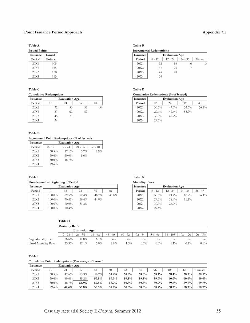
Point Issuance Period Approach Appendix 7.1
Table A Table B
Issued Points Incremental RedemptionsIssuance Issued Issuance Evaluation Age
Period Points Period 0 - 12 12 - 24 24 - 36 36 - 4820X1 105 20X1 32 18 6 320X2 125 20X2 37 25 720X3 150 20X3 45 2820X4 115 20X4 34
Table C Table D
Cumulative Redemptions Cumulative Redemptions (% of Issued)Issuance Evaluation Age Issuance Evaluation Age
Period 12 24 36 48 Period 12 24 36 4820X1 32 50 56 59 20X1 30.5% 47.6% 53.3% 56.2%20X2 37 62 69 20X2 29.6% 49.6% 55.2%20X3 45 73 20X3 30.0% 48.7%20X4 34 20X4 29.6%
Table E
Incremental Point Redemptions (% of Issued)Issuance Evaluation Age
Period 0 - 12 12 - 24 24 - 36 36 - 4820X1 30.5% 17.1% 5.7% 2.9%20X2 29.6% 20.0% 5.6%20X3 30.0% 18.7%20X4 29.6%
Table F Table G
Unredeemed at Beginning of Period Mortality RatesIssuance Evaluation Age Issuance Evaluation Age
Period 0 12 24 36 48 Period 0 - 12 12 - 24 24 - 36 36 - 4820X1 100.0% 69.5% 52.4% 46.7% 43.8% 20X1 30.5% 24.7% 10.9% 6.1%20X2 100.0% 70.4% 50.4% 44.8% 20X2 29.6% 28.4% 11.1%20X3 100.0% 70.0% 51.3% 20X3 30.0% 26.7%20X4 100.0% 70.4% 20X4 29.6%
Table H
Mortality RatesEvaluation Age
12 - 24 24 - 36 36 - 48 48 - 60 60 - 72 72 - 84 84 - 96 96 - 108 108 - 120 120 - UltAvg. Mortality Rate 26.6% 11.0% 6.1% n.a. n.a. n.a. n.a. n.a. n.a. n.a. Fitted Mortality Rate 25.3% 12.1% 5.8% 2.8% 1.3% 0.6% 0.3% 0.1% 0.1% 0.0%
Table I
Cumulative Point Redemptions (Percentage of Issued)Issuance Evaluation Age
Period 12 24 36 48 60 72 84 96 108 120 Ultimate20X1 30.5% 47.6% 53.3% 56.2% 57.4% 58.0% 58.3% 58.4% 58.4% 58.5% 58.5%20X2 29.6% 49.6% 55.2% 57.8% 59.0% 59.5% 59.8% 59.9% 60.0% 60.0% 60.0%20X3 30.0% 48.7% 54.9% 57.5% 58.7% 59.3% 59.5% 59.7% 59.7% 59.7% 59.7%20X4 29.6% 47.4% 53.8% 56.5% 57.7% 58.3% 58.5% 58.7% 58.7% 58.7% 58.7%
Casualty Actuarial Society E-Forum, Summer 2012 35

Aggregate Member Join Period Approach Appendix 7.2
Table A Table B
Cumulative Issued - Aggregate Cumulative Redemptions - AggregateJoin Evaluation Age Join Evaluation Age
Period 12 24 36 48 Period 12 24 36 4820X1 436 445 528 555 20X1 73 192 334 37920X2 525 573 609 20X2 78 214 40120X3 475 486 20X3 90 19320X4 452 20X4 84
Table C Table D
Cumulative Redemption Rates - Aggregate Projected Cumulative Redemption Rates - AggregateJoin Evaluation Age Join Evaluation Age
Period 12 24 36 48 Period 12 24 36 4820X1 16.7% 43.1% 63.3% 68.3% 20X1 16.7% 43.1% 63.3% 68.3%20X2 14.9% 37.3% 65.8% 20X2 14.9% 37.3% 65.8% 68.3%20X3 18.9% 39.7% 20X3 18.9% 39.7% 64.6% 68.3%20X4 18.6% 20X4 18.6% 40.1% 64.6% 68.3%
Casualty Actuarial Society E-Forum, Summer 2012 36

Point Issuance Period Approach Appendix 7.3Redemption Rate on Issued to Redemption Rate on Outstanding Points
Points Ultimate Cumulative Estimated Un-redeemed UltimateIssued Redemption Expected Redeemed Points Points Redemption
Issuance As of Rate On Ultimate Points As of Redeemed As of Rate OnPeriod 12/31/20X4 Issued Redemptions 12/31/20X4 In Future 12/31/20X4 Outstanding
(1) (2) (3) (4) (5) (6) (7) (8)
20X1 105 58.5% 61 59 2 46 5.2%20X2 125 60.0% 75 69 6 56 10.7%20X3 150 59.7% 90 73 17 77 21.6%20X4 115 58.7% 68 34 34 81 41.4%
Total 495 294 235 59 260 22.5%
Notes:(2), (5) From database. (6) (4) - (5).
(3) Estimated ultimate redemptions using PIP method. (7) (2) - (5).(4) (2) x (3). (8) (6) / (7).
Casualty Actuarial Society E-Forum, Summer 2012 37

Value Per Point Redemption Estimation Approaches Appendix 7.4
7.4.1: Value Per Point - Single Redemption Option - Example
Redemption Period1 2 3 4 5
(1) Redemption Pattern 35.0% 30.0% 20.0% 10.0% 5.0%
(2) Value At Time of Redemption $1.00 $0.95 $0.91 $0.86 $0.82
(3) Estimated Weighted Value of Unredeemed Points $0.94
7.4.2: Value Per Point - Multiple Redemption Option - Example
Redemption Period Utilization1 2 3 4 5 (6)
(4) Redemption Pattern 15.0% 15.0% 20.0% 25.0% 25.0%
(5) Value at Time of Redemption:Option A $1.05 $1.10 $1.16 $1.22 $1.20 50.0%
Option B $0.90 $0.99 $1.09 $1.20 $1.32 45.0%
Option C $0.25 $0.25 $0.25 $0.25 $0.25 5.0%
(7) Estimated Weighted Value of Unredeemed Points $1.10
Notes:(3) [ Sumproduct of (1) and (2) at each respective maturity ] / [ Sum of (1) at each respective maturity ]
(7) [ Sum of (4) at each respective maturity ]
[ Sumproduct of (4) and (5) at each respective maturity x (6) for each respective utilization option ]
Casualty Actuarial Society E-Forum, Summer 2012 38

Hypothetical Financial Statements Appendix 7.5¡Burrito Fresco! Page 1Balance Sheet and Statement of Income
Balance Sheet Balance SheetAccrued Cost Approach Deferred Revenue Approach
Beginning End of End of Beginning End of End ofOf Period 1 Period 1 Period 2 Of Period 1 Period 1 Period 2
Cash $0.00 $2,000.00 $4,000.00 $0.00 $2,000.00 $4,000.00Burrito Inventory $2,150.00 $1,150.00 $0.00 $2,150.00 $1,150.00 $0.00
Total Assets $2,150.00 $3,150.00 $4,000.00 $2,150.00 $3,150.00 $4,000.00
Accrued Expenses $0.00 $75.00 $0.00 n.a. n.a. n.a. Deferred Revenue n.a. n.a. n.a. $0.00 $139.53 $0.00
Equity $2,150.00 $3,075.00 $4,000.00 $2,150.00 $3,010.47 $4,000.00
Total Liabilities & Equity $2,150.00 $3,150.00 $4,000.00 $2,150.00 $3,150.00 $4,000.00
Statement of Income Statement of IncomeAccrued Cost Approach Deferred Revenue Approach
Period 1 Period 2 Cumulative Period 1 Period 2 Cumulative
Revenue $2,000.00 $2,000.00 $4,000.00 $1,860.47 $2,139.53 $4,000.00Expenses $1,075.00 $1,075.00 $2,150.00 $1,000.00 $1,150.00 $2,150.00
Net Income $925.00 $925.00 $1,850.00 $860.47 $989.53 $1,850.00
Casualty Actuarial Society E-Forum, Summer 2012 39

Appendix 7.5Page 2
Hypothetical Financial StatementsJournal Entries
Accrued Cost Method
Period 1: Sales and Burrito Point Cost AccrualsSales of Burritos and Issuance of Associated Burrito Points
Db Cash $2,000.00
Cr Revenue $2,000.00
Db Expenses (Cost of Goods Sold) $1,000.00
Cr Burrito Inventory $1,000.00
Db Expenses (Issued Burrito Points) $75.00
Cr Accrued Burrito Point Liability $75.00
Period 2: Sales and Burrito Point Accrued Expenses and Burrito Point RedemptionsSales of Burritos and Issuance of Associated Burrito Points
Db Cash $2,000.00
Cr Revenue $2,000.00
Db Expenses (Cost of Goods Sold) $1,000.00
Cr Burrito Inventory $1,000.00
Db Expenses (Issued Burrito Points) $75.00
Cr Accrued Burrito Point Liability $75.00
Redemptions of Outstanding Burrito Points
Db Accrued Burrito Point Liability $150.00
Cr Burrito Inventory $150.00
Deferred Revenue Method
Period 1: Sales and Burrito Point Deferred RevenueSales of Burritos and Issuance of Associated Burrito Points
Db Cash $2,000.00
Cr Revenue $1,860.47
Cr Deferred Revenue $139.53
Db Expenses (Cost of Goods Sold) $1,000.00
Cr Burrito Inventory $1,000.00
Period 2: Sales and Burrito Point Deferred Revenue and Burrito Point RedemptionsSales of Burritos and Issuance of Associated Burrito Points
Db Cash $2,000.00
Cr Revenue $1,860.47
Cr Deferred Revenue $139.53
Db Expenses (Cost of Goods Sold) $1,000.00
Cr Burrito Inventory $1,000.00
Redemptions of Outstanding Burrito Points
Db Deferred Revenue $279.06
Cr Revenue $279.06
Db Expenses (Cost of Goods Sold) $150.00
Cr Burrito Inventory $150.00
Casualty Actuarial Society E-Forum, Summer 2012 40

Casualty Actuarial Society E-Forum, Summer 2012
A Note on Parameter Risk
By Gary Venter, FCAS, MAAA, CERA, and Rajesh Sahasrabuddhe, FCAS, MAAA1
June 21, 2012
1 The authors wish to thank John A. Major, ASA for his thoughtful and thorough review, with the usual caveat that any errors that remain are the responsibility of the authors.

Contents
1 Introduction 21.1 Sources of Uncertainty . . . . . . . . . . . . . . . . . . . . . . . . 21.2 Principles of Diversification . . . . . . . . . . . . . . . . . . . . . 3
1.2.1 Uncertain Trend Example . . . . . . . . . . . . . . . . . . 4
2 Parameter Estimation Methods 5
3 Parameter Uncertainty Models 63.1 Uncertainty in Regression Parameters . . . . . . . . . . . . . . . 63.2 Uncertainty in Parameters Estimated by Maximum Likelihood . 8
3.2.1 Large Samples . . . . . . . . . . . . . . . . . . . . . . . . 83.2.2 Pareto Example . . . . . . . . . . . . . . . . . . . . . . . 83.2.3 Limited Samples Sizes . . . . . . . . . . . . . . . . . . . . 93.2.4 The Pareto Example . . . . . . . . . . . . . . . . . . . . . 103.2.5 Bayes Theorem . . . . . . . . . . . . . . . . . . . . . . . . 11
3.3 Uncertainty in Model Free Estimators . . . . . . . . . . . . . . . 12
4 Incorporating parameter riskin simulation models 14
5 Conclusion 14
1
A Note on Parameter Risk
Casualty Actuarial Society E-Forum, Summer 2012 1

1 Introduction
For most actuarial modeling applications, model parameters are unknown andmust be estimated. If the associated parameter estimation error is not recog-nized in the modeling, there is a good chance that a substantial portion of theadverse (and favorable) loss potential will appear to be diversified away in theaggregation process.
There is an old fable about buying eggs at 10¢ each and selling them for $1.00per dozen, making up the difference by doing high volume. The misestimationof the required price is not diversified by volume. Rather, it is a systematicrisk that has to be analyzed separately. Similarly parameter risk is a form ofsystematic risk that does not diversify with volume, although it may diversifyacross portfolios to some degree.
1.1 Sources of Uncertainty
Parameter risk is the uncertainty as to whether the parameters are appropriatefor the phenomenon that we are attempting to model. This uncertainty resultsfrom the following factors:
Sampling risk Parameters are estimated from an observed sample. Parameteruncertainty results from differences between that sample and the popula-tion.
Data bias Parameters that are used to model outcomes of events that occurduring an exposure period are estimated from observations from an expe-rience period. We often adjust these observations in an attempt to correctfor differences between the experience and exposure periods. The mostcommon such adjustment is the trending of claims amounts. This ad-justment is intended to remove this bias created by cost level differences.However, if the data are not adjusted correctly then a bias may persistor possibly even be exacerbated. Furthermore, if the amount of the ad-justment itself is uncertain, then it should be treated as an additionalparameter in the model.
The purpose of this Study Note is to demonstrate that for common approachesfor determining mean estimates of actuarial model parameters there exist asso-ciated parameter uncertainty models. These uncertainty models are intended toaddress Sampling Risk. However, this Study Note does not include details re-garding the theory and derivation of those uncertainty models. Readers shouldconsult appropriate sources for that information.
There are (at least) four additional sources of uncertainty that should be rec-ognized.
2
A Note on Parameter Risk
Casualty Actuarial Society E-Forum, Summer 2012 2

Process risk refers to the inherent uncertainty of the insurance claims process.Process risk can diversify away as discussed in Section 1.2.
Model misspecification is the risk that the wrong model is being estimatedand applied. For example, this is the risk that we use an exponentialmodel when the phenomenon follows a Pareto distribution. Insufficientparameter identification is also a type of model misspecification.
Actuarial model risk is a broad form of misspecification risk that resultsfrom the possibility that the entire actuarial modeling framework may notbe appropriate for the phenomenon being modeled. For example, we maymodel ultimate losses using a loss development model when ultimate claimamounts are not proportional to claim amounts as of the valuation date.Discussion of this risk, which may be significant, is beyond the scope ofthis Study Note.
Insufficient parameter identification results when we fail to recognize re-lationships in our models or fail to recognize that certain elements of ourmodel are subject to uncertainty. Examples include:
� Our model may not recognize correlations between development fac-tors in adjacent intervals.
� We may not recognize that relativity between the frequency for aclass and the frequency for a base class is an estimated parameter.
1.2 Principles of Diversification
One ad-hoc adjustment sometimes applied in order to capture parameter risk isto add further spread to the frequency and severity distributions. However thisapproach only adds process risk which will wash out with diversification.
To illustrate the problem, consider applying uncertain trend to the collectiverisk model. Let N be the random variable for the number of claims, and denoteamount of the jth claim as Xj , where the claims amounts are all independentand identically distributed (IID) and independent of N. We then have:
L =N∑j=1
Xj (1.1)
E(L) = E(N)E(X) (1.2)
V ar(L) = E(N)V ar(X) + E(X)2V ar(N) (1.3)
To understand the effect of diversification, consider the coefficient of variation(CV, the ratio of standard deviation to mean) of L as a proxy for model uncer-tainty. It is more convenient to calculate square of the CV s [CV (L)2] which is
3
A Note on Parameter Risk
Casualty Actuarial Society E-Forum, Summer 2012 3

the ratio of the variance divided by the mean squared = V ar(L)/E(L)2:
CV (L)2 =V ar(L)
E(L)2(1.4)
=E(N)V ar(X) + E(X)2V ar(N)
E(N)2E(X)2
=V ar(X)
E(N)E(X)2+V ar(N)
E(N)2(1.5)
Actuaries often assume that the CV is constant for severity distributions.
Likewise, for frequency distributions the ratio of variance to mean is often as-sumed to be constant. We denote that ratio as VM and offer the followingexamples:
� For a Poisson Distribution , VM is equal to 1.
� For the negative binomial distribution with parameters r and β, with meanr and variance r(1 + β), VM is 1 + β, which is often taken as a constantas volume changes.
In any case, VM is constant under the addition of IID exposure units.
By substitution, we have
CV (L)2 =CV (X)2
E(N)+
VM
E(N)(1.6)
The numerators of (1.6) are constant under increase in exposure units and infla-tion, so CV (L)2 decreases proportionally to the inverse of the expected numberof claims, and thus can get quite small as volume increases. This is the problemwith the collective risk model without parameter uncertainty. The volatility canget unrealistically low leading the actuary to believe that there is no risk in largeinsurance portfolios. This is a dangerous conclusion as it would lead the insurerto write more business. If we also consider the risk that models for X and Nmay be incorrectly specified (see the example of the eggs), we understand thatpotential financial loss actually increases with volume.
1.2.1 Uncertain Trend Example
We provide the following example to demonstrate how the aggregate claimsrandom variable is affected by uncertain trend. Including the risk of uncertaintrend or other systematic risk will put a minimum on CV (L) that cannot bereduced by diversification (i.e. it is not inversely proportional to E(N)).
Let J denote a random trend factor with mean 1.00. We then have the followingrelationships:
4
A Note on Parameter Risk
Casualty Actuarial Society E-Forum, Summer 2012 4

E(J) = 1 (1.7)
CV (J)2 =V ar(J)
E(J)2
= V ar(J) (1.8)
Our claims model and its characteristic functions for the trended claim amountK may be expressed as follows:
K = JL (1.9)
E(K) = E(JL)
= E(J)E(L)
= E(L) (1.10)
V ar(K) = V ar(JL)
= E(J)2V ar(L) + E(L)2V ar(J) + V ar(J)V ar(L)
= V ar(L) + E(L)2CV (J)2 + CV (J)2V ar(L) (1.11)
CV (K)2 =V ar(L) + E(L)2CV (J)2 + CV (J)2V ar(L)
E(L)2
= CV (L)2 + CV (J)2 + CV (L)2 × CV (J)2 (1.12)
We can now observe that CV (K) has a minimum of CV (J) even if CV (L)2
goes to zero (as E(N) is large). That is, the uncertainty in the trend parameteris not diversified away.
2 Parameter Estimation Methods
We address three common approaches of parameter estimation in this StudyNote. For the first two approaches there is a formal methodology for modelingthe distribution of parameter fitting errors. This provides quantification ofestimation risk.
Regression analysis is used to estimate the parameters of a dependency rela-tionship. Although the category of regression analysis includes non-linearapproaches, this Study Note focuses on linear approaches.
5
A Note on Parameter Risk
Casualty Actuarial Society E-Forum, Summer 2012 5

Maximum likelihood estimation is most commonly used in estimating fre-quency and severity distributions. The resulting parameters are referredto as maximum likelihood estimators (MLEs).
Although the last approach is less formal, it is no less subject to parameter riskand in fact, it may be subject to greater parameter risk.
Model free methods are commonly used by actuaries in certain applicationssuch as estimation of claim development factors.
3 Parameter Uncertainty Models
3.1 Uncertainty in Regression Parameters
When the data displays dependencies and is (approximately) normally dis-tributed after accounting for those dependencies, actuaries will often use re-gression to estimate parameters. A common example exists with the modelingof the relationship between claim amounts (X ) and time (t) which is oftenmodeled using the following relationship:
Yi = lnXi = β0 + β1ti + εi (3.1)
where β0 is often referred to as the intercept and β1 is often referred to as theslope or regression coefficient.
We observe the following about this relationship:
� Using the log-transform of claim amounts implies that claim values are log-normally distributed. This may be appropriate if the Xis are individualclaim observations but possibly not if they are averages.
It also implies that the growth in claim amounts is exponential rather thanlinear. This is a generally accepted assumption.
� Exponentiation of the regression coefficient β1 less unity (i.e. eβ1 − 1)represents an estimate of the annual rate of severity trend.
� E(Yi|ti) = β0 + β1ti, often written as µi, is the mean of the distributionof the logs of the claim amounts at time ti.
We should recognize that regression techniques not only provide estimates ofparameters such as β1 and quantities such as µi but also the uncertainty of thoseestimates. More specifically, for a regression on N data points, the estimatedstandard deviation of the regression error term, εi, of the regression may beexpressed as:
σy =
√SSE
N − 2(3.2)
6
A Note on Parameter Risk
Casualty Actuarial Society E-Forum, Summer 2012 6

We denote the sample standard deviation1 of the observed times (tis) as σt. Theestimators then have the following properties which are discussed in textbookson regression.
� The standard error of b1 (the estimator of β1) may be estimated as
σb1 =σy
σt√N − 1
. (3.3)
The residuals of b1 after subtracting β1 and scaling by the standard errorof b1 follow a Student’s t-distribution with N − 2 degrees of freedom.
� The (1− α)% confidence interval is equal to
b1 ± tN−2,1−α2σb1 (3.4)
� The standard error of mi, the estimator of µi obtained by substituting bsfor βs, is calculated as follows:
σµi = σy
√1 +
1
N+
(ti − t)2(N − 1)σ2
t
(3.5)
Similar to equation 3.3, the scaled residuals of µi also follow Student’st-distribution with N -2 degrees of freedom.
- We can observe that, as N becomes large, σµi approaches σy.
- The standard error increases as ti is further from t.
- The (1− α)% prediction interval is equal to
Yi ± tN−2,1−α2σµi (3.6)
Particularly when fitting regression models to average values, N (and, by ex-tension, (N − 2)) may be “small” which leads to a Student’s t-distribution withconsiderable dispersion. This may result in “unreasonable” parameter values forthe regression parameters at higher or lower percentile levels. Excessive disper-sion of estimators of parameters is consistent with lack of statistical significanceof regression parameters. Issues related to the significance of regression parame-ters are outside the scope of this Study Note. Readers should consult textbookson regression analysis for the derivation of the formulae above or for a morecomplete understanding of the development of the uncertainty model.
1This is the unbiased standard deviation with denominator N − 1.
7
A Note on Parameter Risk
Casualty Actuarial Society E-Forum, Summer 2012 7

3.2 Uncertainty in Parameters Estimated by MaximumLikelihood
The likelihood function (L) represents the probability that a sample is observedgiven a model and parameters. It is calculated as the product of probabilityfunctions in the discrete case or density functions in the continuous case. Asit is computationally more efficient, we generally work with the negative of thelog-likelihood (NLL) which is the negative value of the sum of the logarithmsof the probability (density) functions . Specifically for a continuous model withdensity function f , we have:
L(x; θ) =∏
f(xi) (3.7)
NLL(x; θ) = −∑
ln f(xi) (3.8)
The maximum of L occurs at the minimum of NLL. The minimum of NLL canoften be calculated by setting its derivatives with respect to the parameters ofthe probability (density) function to zero and solving for the parameters. How-ever in more complicated models the minimization must be done numerically.
3.2.1 Large Samples
As described in Loss Models [2], for large N , the distribution of the parameterestimates is asymptotically normal and the inverse of the Hessian matrix(also referred to as the Hessian and denoted H ) provides the variances andcovariances of the parameters. The Hessian is comprised of the second partialderivatives of a function of interest, in this case the NLL. The Hessian of theNLL function is also referred to as the information matrix.2
3.2.2 Pareto Example
In this section, we demonstrate the calculation for the Pareto distribution withthe following properties:
F (x) = 1− x−α (3.9)
f(x) = αx−α−1 (3.10)
ln(f(x)) = ln(α) + (−α− 1) ln(x) (3.11)
2Most optimization software will numerically calculate the information matrix.
8
A Note on Parameter Risk
Casualty Actuarial Society E-Forum, Summer 2012 8

We then calculate the NLL as follows:
NLL = −n∑i=1
ln f(xi)
= −n∑i=1
(ln(α) + (−α− 1) ln(xi))
= −n∑i=1
ln(α) + (α+ 1)n∑i=1
ln(xi)
= −nln(α) + (α+ 1)n∑i=1
ln(xi) (3.12)
To solve for the MLE of α, we taking the derivative of the NLL with respectto α and solve:
dNLL
dα=−nα
+n∑i=1
ln(xi) = 0
α =n∑n
i=1 ln(xi)(3.13)
To determine the variance of the MLE, we take second partial derivatives of theNLL as follows:
∂2NLL
∂α2=
n
α2(3.14)
With only one parameter, the H is a 1× 1 matrix.
H =[
nα2
](3.15)
H−1 =[
α2
n
](3.16)
So for large n, the maximum likelihood estimator of the Pareto parameter isnormally distributed with mean = α and estimated variance = α2/n.
�
We leave it to the reader to verify the uncertainty models for the exponentialand lognormal distributions below.
3.2.3 Limited Samples Sizes
For insurance samples the sample size is usually not asymptotic to infinity andthe normal distribution often is inappropriate. For instance, a normal distribu-tion might imply too high a probability of negative values for parameters and
9
A Note on Parameter Risk
Casualty Actuarial Society E-Forum, Summer 2012 9

Table 1: Examples
Model Lognormal(µ, σ) exponential(λ)
Mean eµ+σ2/2 1/λ
MLE µ =
∑lnxin
, λ =n∑xi
σ =
∑(lnxi − µ)2
n
H
n
σ20
02n
σ2
n
λ2
H−1
σ2
n0
0σ2
2n
λ2
n
functions of parameters that have to be positive. A reasonable alternative inthat case is to use the gamma distribution for each parameter, with the cor-relation structure of the multivariate normal. This can be implemented usingthe normal copula with gamma marginal distributions. As the sample sizes getlarger, the gamma approaches the normal, so using it is consistent with theasymptotic theory.
3.2.4 The Pareto Example
Returning to our Pareto example, we recall that the log of a Pareto variate isexponentially distributed and the sum of exponentials is gamma. From 3.13,we recognize that the Pareto variates are in the denominator of the MLE ofα. As a result, we understand that α is inverse gamma distributed with meanand variance of estimators being α and α2/n, respectively. This agrees whatwas calculated is Section 3.2.2. The associated inverse gamma shape and scaleparameters would be n+ 2 and α(n+ 1), respectively.
It would be tempting to use this inverse gamma as the distribution of the trueparameter given the fit. However it is just the opposite - that inverse gammais the distribution of the estimator given the true parameter. Especially withskewed distributions like the inverse gamma, these two distributions are not thesame.
This is a natural setup for Bayesian analysis. We know the distribution of the
10
A Note on Parameter Risk
Casualty Actuarial Society E-Forum, Summer 2012 10

estimator given the parameters but want the distribution of the parametersgiven the estimator. If the MLE were also the Bayes estimate from some priordistribution of the parameters, then Bayes Theorem would provide the posteriordistribution of the parameters given the estimate. This happens in one setting,and the resulting posterior distribution of the parameters turns out to be gammain that case.
3.2.5 Bayes Theorem
Bayes Theorem provides a formula for the posterior distribution for Y given X,using the distributions of X, Y and X given Y . That is:
f(Y |X) = f(X|Y )f(Y )
f(X)(3.17)
We can think of Y as the true parameter, which is considered a random variablesince it is not known, and X as the data. Then, the prior distribution ofY is f(Y ) and f(X|Y ) is the conditional distribution of the data given theparameter. We want to find the conditional distribution of Y given X, and inthat context f(X) in equation 3.17 can be considered as a normalizing constant(not a function of Y) needed to make the distribution integrate to unity. Assuch, Bayes Theorem can also be expressed as:
f(Y |X) ∝ f(X|Y )f(Y ) (3.18)
Where ∝ indicates proportionality - meaning equal up to factors not containingY . This formulation allows the use of so-called non-informative priors - such as,in this case f(Y ). The prior f(Y ) is thus expressed by suppressing factors notcontaining Y . This allows the prior f(Y ) itself to be expressed up to a constantfactor, and in fact does not even have to integrate to a finite number as longas f(Y |X) does. This gives the possibility of prior distributions that are veryspread out on the real line and so have little or no impact on the estimatedparameters.
Common examples are f(Y ) ∝ 1 on the whole real line, or f(Y ) ∝ 1/Y on thepositive reals. These can be expressed as limits of the same distributions on(−M,M) or (1/M,M) as M grows without limit. Thus they are very diffuse.Such non-informative priors can give insights into the estimation uncertainty.
For the Pareto, the prior is for the parameter α, and for a positive parametera useful non-informative prior is f(α) ∝ 1/α . The anti-derivative of this prioris ln(α), which slowly diverges at both ends of the positive real line. Thus ithas infinite weight at both ends of the range, and as a result does not biasthe parameter either up or down. In comparison, for a positive parameter, theprior f(α) ∝ 1 only diverges at the right end of the range, and tends to pullparameters up.
11
A Note on Parameter Risk
Casualty Actuarial Society E-Forum, Summer 2012 11

In this example f(X|α) is the distribution of the observations given α. If P isthe product of the observations, it is easy to show that
f(X|α) ∝ αn/Pα+1 (3.19)
If we substitute β = −ln1/P , we have:
f(X|α) ∝ αn exp (−βα) (3.20)
Comparing this to the gamma density shows that the distribution of the param-eter given the data is a gamma distribution with shape parameter n and mean= 1/average[lnxj ]. This mean is the MLE for α, which supports the use of thisparticular non-informative prior. This gamma distribution is thus the posteriordistribution for the true α, with mean equal to the MLE estimate.
A similar exercise for the Poisson with mean λ and n samples which have sumof observations S gives a gamma posterior distribution for λ with mean S/nand shape parameter S. This again agrees with the MLE and has a gammadistribution for the true parameter. Both examples support the idea of usinggamma distributions for the parameter uncertainty.
3.3 Uncertainty in Model Free Estimators
Development factors can be calculated within a parametric or model-free frame-work. The factors themselves are parameters, but the distinction is whether ornot a distribution is assumed for the deviation of the losses from what would beestimated by applying the factors, that is, for the distribution of the residualsof the development factor approach.
One method for quantifying the estimation errors of the factors is bootstrapping.This method resamples the residuals and uses them to create new, artificialtriangles. The factors are repeatedly estimated from these artificial triangles,and an empirical distribution of the factors is thus built up. Bootstrapping is astraightforward approach but has potential pitfalls that require some care.
� For example, it should be recognized that there are a different number ofobservations used in the estimation of successive incremental developmentfactors, so each “parameter” has its own number of degrees of freedom.The degrees of freedom is an input to the resampling process.
In nonlinear models, the degrees of freedom can be estimated by Ye’smethod of generalized degrees of freedom[3] (gdf). The gdf for an observedpoint, for an estimation procedure, is the derivative of the fitted point withrespect to the observed point. If that derivative is one, the observed pointhas the power to pull the model to it with an exact match. This wouldshow up for instance in fitting a quintic polynomial to 6 points, whichit can fit exactly, using up all the degrees of freedom. The gdf agrees
12
A Note on Parameter Risk
Casualty Actuarial Society E-Forum, Summer 2012 12

with the usual notion of degrees of freedom in linear models, and is moreappropriate in nonlinear models.
Even when using the gdf degrees of freedom for each point’s residual, how-ever, bootstrapping is regarded as unreliable in small samples (e.g., lessthan 40 observations per fitted parameter). There are too few residualsto get a representative resample. This leads to the method of parametricbootstrapping, which draws from fitted distributions instead of the ob-served residuals. This would only be applicable in the case where thereis a parametric model for the residuals. For instance, if residuals are as-sumed to be over-dispersed Poisson, resampling can be done from thisdistribution.
� The approach outlined in England and Verall (2002) uses Pearson residu-als, rp, which are calculated using the following approach:
rp =observation− estimated parameter
estimated parameter1/2(3.21)
� A technical problem is that bootstrapping gives the distribution of theestimated parameters given the true parameters, but what is needed isthe distribution of the true parameters given the estimated parameters.This difference will be important especially with asymmetric distributions.This is the same problem that was encountered in the Pareto example,and which there led to replacing the inverse gamma distribution by thegamma. This is a known problem with bootstrapping which is addressedin textbooks on the subject, but is beyond the scope of this Study Note.
� In development triangles another pitfall of resampling is that the modelmight not hold for the data.
- For instance, in slowly developing lines, the first report claim amountsmight often be near zero. The second report might then be wellmodeled as a constant (for the initial valuation of claims that aretrue IBNR at the first report) plus a factor times first report (fordevelopment of the small number of reported claims). If the modeluses just a factor, there might be some very high observed factors thatwould not apply in general but might when the first report is verylow. Resampling can generate obviously inappropriate developmentin this case - such as a large residual combined with a large initialvalue - basically because the wrong model is being used to estimateclaims at second report.
- Also if there are calendar-year effects in the data but not in themodel, bootstrapping can again be distorted because it is resamplingresiduals of a model that does not apply.
If the development factors are estimated by MLE from a parametric model,the inverse of the Hessian (information matrix) can be used to quantify the
13
A Note on Parameter Risk
Casualty Actuarial Society E-Forum, Summer 2012 13

parameter uncertainty in the factors, just as in any other MLE case. Clark(2006)[1] gives an example of this. Comparison studies have found the results of thismethod to be comparable to bootstrapping the parameter uncertainty, and usingthe information matrix in this way avoids many of the pitfalls of bootstrapping.
4 Incorporating parameter riskin simulation models
Actuaries typically use simulation to model risk and uncertainty. Parameter es-timation is easily incorporated in a simulation through a two-stage process: ineach scenario, we first simulate the parameters from the parameter-risk distribu-tions, and then simulate the process from the simulated parameters. Examplesof this approach are as follows:
� In our example of uncertain trend from Section 2, we would first simulateaggregate claims from the collective risk model, and then simulate J whichis then multiplied by the aggregate claims. This approach results in asimilar floor imposed on the simulated claims CV (K).
� In our Pareto example, we first simulate the parameter value and thensimulate claims based on that parameter.
Even if the process risk diversifies away, the parameter risk will not.
5 Conclusion
It should be noted that this approach assumes that:
Parameter risk is one of the principal elements that have to be quantified toobtain reasonable representations of risky processes. As we demonstrated, ina loss simulation environment, simulating from the collective risk model with-out recognizing parameter risk can wash out most of the actual risk. This isparticularly true for high-volume lines.
In this Study Note, we have provided an overview of approaches to estimateparameter uncertainty based on the manner in which the parameters are esti-mated. Interested readers should consult textbooks and other papers for detailsrelated to the theory on the parameter uncertainty models.
References
[1] David R. Clark. Variance and covariance due to inflation. Casualty ActuarialSociety Forum, pages 61–95, Fall 2006.
14
A Note on Parameter Risk
Casualty Actuarial Society E-Forum, Summer 2012 14

[2] Harry H. Panjer Klugman, Stuart A. and Gordon E. Willmot. Loss Models:From Data to Decisions. Wiley, third edition, 2008.
[3] Jianming Ye. On measuring and correcting the effects of data mining andmodel selection. Journal of the American Statistical Association, pages 120–131, March 1998.
15
A Note on Parameter Risk
Casualty Actuarial Society E-Forum, Summer 2012 15