Caste in Class: Evidence from Peers and Teachers
53
CENTRO DE ESTUDIOS MONETARIOS Y FINANCIEROS www.cemfi.es September 2020 working paper 2018 Casado del Alisal 5, 28014 Madrid, Spain Caste in Class: Evidence from Peers and Teachers Javier García-Brazales
Transcript of Caste in Class: Evidence from Peers and Teachers

CENTRO DE ESTUDIOSMONETARIOS Y FINANCIEROS
www.cemfi.es
September 2020
working paper2018
Casado del Alisal 5, 28014 Madrid, Spain
Caste in Class:Evidence from Peers
and Teachers
Javier García-Brazales

Keywords: Castes, peer effects, non-cognitive skills, India.
Javier García-BrazalesCEMFI
Differences in academic achievement across Indian castes are both large and persistent. I makeuse of rich individual data to explore how class caste composition affects academic progress aswell as the mechanisms in place. Benefiting from exogenous assignment of students to classesand teachers, I find that a one-percentage point increase in the proportion of low-caste class-mates leads to a fall of around 2% of a standard deviation in the mathematics score and to muchsmaller effects in English. This phenomenon is mediated through lower effort exerted by thestudents, which itself emanates from the students' worsened perception about the extent to whichtheir teachers value them. This non-cognitive channel, which has not been previously identified inthe peer effects literature, suggests that the use of a fairly malleable input such as more open andreceptive teachers among low-caste students would be an appropriate policy response.
CEMFI Working Paper No. 2018September 2020
Caste in Class: Evidence from Peers and Teachers
Abstract
JEL Codes: I24, J15, J24.

Acknowledgement
The author gratefully acknowledges the funding received from the Fundación Ramón Areces. Thedata used in this publication come from Young Lives, a 15-year study of the changing nature ofchildhood poverty in Ethiopia, India, Peru and Vietnam (www.younglives.org.uk). Young Lives isfunded by UK aid from the Department for International Development (DFID). The views expressedhere are those of the author. They are not necessarily those of Young Lives, the University ofOxford, DFID or other funders.

1 Introduction
One of the distinctive features of the Indian society is its caste system. It is a hereditary con-
struction that plays a role in about every aspect of daily life and comes hand-in-hand with large
inequalities in multiple dimensions between low and high castes (Kijima, 2006). One of them
is school achievement. Similarly to the white-black gap in the United States, sizable di↵erences
in school enrollment and test scores between high and low castes have been present for decades
and, despite a recent narrowing, remain strong nowadays (e.g. Bertrand et al., 2010). Given the
importance of understanding the roots of this gap in order to design optimal policies that can
reduce the existing academic di↵erences and the inequalities in income and wealth across castes
that perpetuate later in life, the lack of formal research on the relative academic circumstances of
low and high castes and on their dynamic evolution constitutes an important gap in the literature
(Munshi, 2019).
One such policy, launched five decades ago, consisted in putting in place the world’s largest
a�rmative action program to ensure that lower castes would have access to a fixed percentage
of reserved seats in university and in public servant positions.1 A series of recent papers shows
that this initiative has been partly successful: Bagde et al. (2016) find that these programs do
bring a higher proportion of low-caste students into college education at engineering schools while
Bhattacharjee (2016) claims that this is also true for Other Backward Castes. Khanna (2016)
shows that the beneficial e↵ects for low-caste students participating in these programs extends to
their ability to find jobs.
While these findings shed some light on the extent to which low-caste students benefit from
a�rmative action in terms of targeting and proper matching of these policies as described in Munshi
(2019), formal research around the potential catching-up experienced by low-caste students during
the course of the studies and the mechanisms through which these policies work is very scarce.
In particular, an important question remains unexplored: what is the role of classroom mix-caste
composition on academic and non-cognitive abilities of both lower and higher caste individuals, and
how do teachers play a role in moderating or exacerbating these e↵ects?2 Although some work has
postulated that positive peer e↵ects favoring disadvantaged groups should be present when mixed
with higher-caste students (Kochar et al., 2008) this is not ex-ante obvious, particularly given the
1Originally, these policies targeted the lowest castes (Scheduled Castes and Scheduled Tribes), but were subsequently ex-
panded to Other Backward Castes. This expansion was recommended by the Mandal Commission of 1980, and was implemented
in college in 2006. Since the objective of these policies is to bring the caste composition in higher education closer to the overall
one in the society, caste-reserved seats amount to around 50% of the available ones: 15% for Scheduled Castes, 7.5% for
Schedules Tribes and 27% for Other Backward Castes.2To the best of my knowledge, only two contemporaneous papers in the peer e↵ects literature have had access to changes
in teacher practices as a response to class composition: Fruehwirth and Gagete-Miranda (2019) and Gong et al. (2019). While
Fruehwirth and Gagete-Miranda (2019) focuses on a very di↵erent setting (kindergarten students in the US), Gong et al.’s
interest is in peers’ gender, which may likely operate very di↵erently from caste e↵ects.
2

existing evidence on lower performance under negative stereotypes (e.g. Hanna and Linden, 2012)
and on unequal teacher treatment of di↵erent castes (e.g. Rawal et al., 2010).
While the a�rmative action programs just described are targeted at the tertiary level, caste-
mixing is not uncommon at earlier stages. The objective of this paper is to answer the above
question by being the first one to feature classroom caste composition into an academic production
function at middle-school. I do this by exploiting the 2016 Indian School Survey module contained
within Oxford University’s Young Lives dataset. It collects cognitive and non-cognitive informa-
tion at the beginning and at the end of one academic year for all the students in all the classes in
Grade 9 within a close-to-representative set of schools in the Indian state of Andhra Pradesh. Im-
portantly, it identifies classmates and teachers and provides detailed individual socio-demographic
information of both groups. Moreover, it collects information on the procedure followed by the
schools when deciding the student composition of each section3. This wealth of information is cru-
cial for exploring potential channels as well as for overcoming the well-known di�culties in proper
identification of peer e↵ects that have plagued the literature (Manski, 1993).
Investigating the exact mechanisms is important. For example, it may be that low caste
status is correlated with lower family investments on education that can spillover to classmates,
or that teachers respond to the caste composition of their students so that there is an optimal
assignment of students to teachers based on caste. Knowing which channels are operating may
contribute to closing the achievement gap. Surprisingly, the lack of evidence on peer e↵ects and
teacher e↵ectiveness in India is not exclusive to the caste dimension - for example, although the
Government recently favored a large push to foster the presence of female teachers, nothing was
known at the time of the implementation about how matched teacher-student gender could help
females to close the existing gap in scores (Muralidharan and Sheth, 2016). This highlights the
extent to which the Indian educational context is under-researched. This paper aims at making
progress along several dimensions.
First, it focuses on the unexplored topic of caste peer e↵ects and looks into their role in cognitive
and non-cognitive performance at school. This allows me to provide novel evidence on academic
disparities across castes not only statically at a given point in time, but also dynamically over
one academic year as well as and on the factors a↵ecting the evolution of the caste gap. This is
relevant, among other reasons, because optimal class formation can make a sizable di↵erence in
the world’s largest school system - over 230 million students enrolled up to Grade 124.
Second, it complements the existing research discussed above on the e↵ectiveness of a�rmative
action programs by taking into consideration the e↵ects of caste composition on the academic
progress of the di↵erent caste subgroups within a classroom as well as teachers’ behavioral re-
3I use the terms class and section interchangeably.4Figure reported in the 2013 All India Education Survey.
3

sponses. Given that changes in class composition arise mechanically in a�rmative action pro-
grams, understanding their e↵ects on both students benefiting from these programs and those that
were not admitted through the policy is relevant when evaluating the overall e↵ectiveness of the
programs.
Third, the richness of my data allows me to carefully explore the potential channels that may
be behind caste peer e↵ects. These include, inter alia, non-cognitive responses from the students
and teachers’ changes in behavior and/or teaching style. Standard datasets for developed countries
lack this information, let alone for developing ones. This has severely limited the exploration of
the full set of potential mechanisms through which peer e↵ects operate, hence leaving room for
alternative channels to be in place even when the authors find evidence for the presence of a specific
one (e.g. Lavy and Schlosser, 2011). Providing this novel look into the student and teacher factors
that significantly contribute to the students’ human capital accumulation is important in light of
the small academic progression and the large disparities in academic trajectories observed in the
Indian context (Singh, 2016).
Fourth, my identification of peer e↵ects is arguably credible and straightforward. My data
provide information on the assignment procedure of students to classes. This allows me to work
with a subsample of classrooms to which the allocation of students is plausibly exogenous (i.e.
headmasters state that the assignment was “random” or “by gender”). I verify this through
detailed balance checks of baseline characteristics. This quasi-randomized setup that I exploit is
uncommon in educational settings across the world, particularly in middle-school5. Because class
e↵ects may be di↵erent at di↵erent ages, being among the first papers that credibly explores them
for middle school is already a relevant contribution. Importantly in terms of external validity, I
show that the qualitative results found for my preferred subsample also hold when expanding the
analysis to classrooms with other, less exogenous, allocation procedures.
By using school fixed e↵ects to account for selection into schools, and by showing that teachers
do not select into classes either, my estimation strategy overcomes the main threats to identifica-
tion. Moreover, having access to scores both at the beginning and at the end of the year allows for
estimating value-added regressions, which are more informative of the role of the current peers and
also allow to control for selection by ability or past investments on the child (Muralidharan and
Sheth, 2016). The fact that the exams are multiple-choice and externally distributed and graded
alleviates concerns of di↵erential grading across castes6. Furthermore, unlike most peer e↵ects pa-
pers that make use of random assignment to peers, which focus on a single school (e.g. Sacerdote,
5Exceptions are South Korea (Kang, 2007) and China (e.g. Carman and Zhang, 2012; Gong et al., 2018),6This avoids the need of using class fixed e↵ects to only resort to within-class variation in performance as in Fairlie et al.
(2014).
4

2001; Zimmerman, 2003), my data were originally designed to be almost representative7 of the
predominantly rural state of Andhra Pradesh. For this reason, I observe schools with di↵erent
types of ownership (e.g. governmental, private aided, private unaided...) located in both rural and
urban areas. This yields results that are arguably more externally valid.
Lastly, the dataset matches students to classmates and instructors, which allows not only to
consider teachers as a mechanism through which peer e↵ects may operate, but also for a narrower
definition of peers compared to the studies that use variation within schools in peer composition
over repeated cross-sections and that are constrained to define as peers all the students in the
same school and grade8. In my preferred specification, and following the existing evidence of close
network formation within castes (e.g. Brown, 2017; Lowe, 2018), I define peers in an even finer
manner: same-caste classmates. This choice, although potentially misclassifying some same-caste
classmates as peers, has the benefit of overcoming selection into peers conditional on students being
in the same class and also avoids the need for modelling a first stage of friendship formation. In
particular, improving on the industry-standard excessively-broad definitions of peers is important
to mitigate the downward bias arising from such measurement error (Arcidiacono et al., 2012).
My paper contributes to several strands of the literature. Most broadly, it connects with
the large literature on peer e↵ects in educational settings (e.g. Hoxby, 2000; Ammermueller and
Pischke, 2009), in particular those exploring contextual peer e↵ects arising from peers’ gender
and racial composition (e.g. Hanushek et al., 2009; Gong et al., 2019) in a (quasi-) randomized
setting (e.g. Kang, 2007; Carrell et al., 2009), and to the much more scarce literature that refers
to developing countries (e.g. De Melo, 2014; Gong et al., 2018).
Instead of the widely discussed gender and racial composition, it investigates a particular feature
of the Indian society, the caste system, that has not been previously explored in the context of
academic peer e↵ects. In this sense, it is closer to a broader literature looking into caste networks
(e.g. Banerjee et al., 2013; Lowe, 2018), interactions across castes (e.g. Munshi and Rosenzweig,
2016; Field et al., 2016), school performance under caste stereotyping (Ho↵ and Pandey, 2006), and
the e↵ect of class interactions between rich and poor children in India (Rao, 2019). Furthermore,
the availability of non-cognitive data allows not only for exploring the e↵ects of peers on non-
cognition, but also the investigation of potential mechanisms. This is important because, in spite
of the wealth of papers on peer e↵ects, these two aspects have largely been obviated due to data
limitations (as argued in, for instance, Lavy et al., 2011; Gong et al., 2018). In fact, my results
suggest a new channel in the literature of peer e↵ects: a fall in the confidence that students have
in that their teachers care for and value them (albeit the teachers do not claim to behave in this
7It is representative of the 95% non-wealthiest households in the province (pro-poor approach).8In reality one expects the majority of interactions with peers to occur at the class level and, most likely, at an even finer
level.
5

way) leads them to exert less e↵ort at school. Hence, this paper also speaks to the literature on the
education production function (a recent review can be found in Jackson et al., 2014) and on teacher
e↵ectiveness, which has been often referred to as the most important school input (e.g. Burgess,
2016). In particular, I provide novel evidence on the role of teacher practices and behaviors in
a↵ecting students’ attitudes with respect to school, especially for stereotyped students (e.g. Hanna
and Linden, 2012; Burgess and Greaves, 2013).
The main finding is that classes with a higher proportion of low-caste students progress sig-
nificantly less over one academic year, particularly in mathematics, for which a one percentage
point increase in the percentage of low-caste students is associated with a fall of 2% of a standard
deviation in the progression of scores. This e↵ect is present above and beyond those generated
by other socio-demographic characteristics correlated with caste and is robust to the inclusion
of a rich set of controls for peer characteristics featuring, among others, wealth, baseline cogni-
tion and non-cognition, health, and parental education. An exploration of the channels suggests
that these e↵ects come from behavioral responses of the students, who feel less valued by their
teachers and lower their academic aspirations. Importantly, this finding that (the perception of)
prejudices by students matters for performance may apply to contexts other than castes, such as
female performance in STEM subjects being a↵ected by lower expectations on their capabilities.
When separating the e↵ects by child’s caste, lower-caste students do not su↵er as much as higher-
caste students when mixed with a higher proportion of low-caste students, which lends support
in an outside-the-lab context to Ho↵ and Pandey (2006)’s work on performance under negative
stereotyping. Finally, while non-linearities seem to be present, other heterogeneous e↵ects are not.
The rest of the paper is organized as follows. Section 2 describes the data used and demonstrates
that there is exogenous assignment of students and teachers to classes within my restricted sample.
Section 3 describes the empirical strategy that I employ to estimate the causal impact of caste class
composition on students’ cognitive evolution, while Section 4 compiles the main results obtained
from it. Section 5 investigates potential mechanisms that may be operating behind my findings
and quantifies their relative importance. Section 6 briefly explores heterogeneous e↵ects and non-
linearities while Section 7 verifies the robustness of my results. Section 8 concludes.
2 Context and Data
2.1 Cultural and Schooling Context
Hindus’ social stratification into four hierarchical classes (varnas) intimately linked to the four
main professions has been in placed over three millennia. Within these classes there are thousands
of castes (jatis). Although being precise about an individual’s jati is crucial when exploring social
6

networks, when evaluating broader phenomena and policies (e.g. discrimination, a�rmative action
programs) the usual level of aggregation relies on a hierarchical system dating back to the British
colonial times that aimed at simplifying the system by distinguishing between: i) Scheduled Castes
(SC), Scheduled Tribes (ST), Other Backward Castes (OBC), and General Castes (GC). While the
first three classes have been traditionally disadvantaged, there are di↵erences across them. Notably,
STs are more socially and geographically isolated while OBCs constitute a more recent addition
to the classification and tend to occupy a middle-ground between SC-STs and GCs (Deshpande et
al., 2014). As conventional in the literature (e.g. Hnatkovska et al., 2013), throughout the analysis
I will use the term “low caste” to refer to individuals belonging to SC or ST.
Given the rural nature of a significant part of my sample it is important to understand castes’
geographical patterns. Data from the Rural Economic and Demographic Survey (REDS) shows
that, for the average Indian village size of 340 households, 30 of them will belong to a given
caste. In recent years there has been a governmental focus to provide a physical school within
walking distance in rural areas. This, coupled with the geographical dispersion of castes, leads to
some degree of caste segregation across schools, particularly in the mixing of GC and low-caste
students (mostly ST). However, cross-caste classroom sharing is not uncommon - and it is often
accompanied by discrimination in access to resources and treatment against low-caste students as
discussed below. Section 2.2 will quantify the extent of caste-mixing within my estimating sample.
The preceding paragraph highlights the importance of taking into account selection of students
into schools when exploring peer e↵ects. I deal with this by including school fixed e↵ects, which
also accounts for varying school quality. However, it may still be possible that there is selection
of students into classes based on unobservables. There are no country-wide regulations regarding
how headmasters should distribute students across classes. As a result, several methods are used:
by randomization, by ability, by last name, by language of instruction, etc. In the next section I
explain how I make use of a question asking headmasters about the way in which each section’s
composition was decided to ensure that my empirical analysis is performed only for the subset of
sections where such composition is plausibly exogenous. One last remark is that once individuals
are assigned to a section they remain with the same classmates for all the subjects in the current
academic year, which are usually delivered by subject-specific teachers.
2.2 Data
My data come from the Young Lives study led by Oxford University, which followed two cohorts of
children (aged 1 and 7 by the time of the first round) across five di↵erent waves from 2002 to 2016
in four countries (India, Peru, Ethiopia, and Vietnam). Apart from collecting data for this panel,
a complementary study, called “School Survey”, was conducted in 2016 to better understand the
7

importance of key educational inputs. To do so, it surveyed a subset of the Young Lives participants
as well as all the students in their same school and grade (Grade 9).9 In this paper I only make
use of the 2016 Indian School Survey.
This dataset is unique in that it not only provides information on basic socio-demographic
characteristics such as gender, age, academic history, family wealth, parental education, and caste,
but it also features rich cognitive and non-cognitive information. Mathematics and English tests
were taken both at the beginning and at the end of the academic year. This permits the estimation
of value added models (that control for baseline cognition), which have a clearer interpretation of
the role of each input over a well-defined period of time and also allow to control for ability and past
investments on the children (Singh, 2015). Importantly, since the baseline cognition is computed at
the beginning of the year (and not at the end of the previous academic year), we overcome concerns
of di↵erential extents of knowledge losses over the holidays (Borman and Boulay, 2004). Moreover,
because the exams are standardized and evaluated by objective external examiners there are less
concerns about the comparability of scores and grading criteria across schools and classes (which
would then be compounded by di↵erential grading depending on student caste as found by Hanna
and Linden, 2012). The availability of the detailed set of individual characteristics (particularly
wealth and non-cognition) is crucial for the credibility of the conditional exogeneity assumption of
caste composition (Luke and Munshi, 2011).10
Cognitive data for mathematics and English come from multiple-choice low-stakes tests of 40
and 50 questions, respectively. I standardize the first-round scores to have a mean of 500 and
a standard deviation of 100. To make round 2 scores directly comparable, I follow Moore et al.
(2017) in using round 1’s mean and standard deviation to standardize the scores from the second
round. In doing so we observe an increase of 30 points in the average mathematics score and a
much more modest one of 6 in English. For this reason, and because peer e↵ects are much weaker
in size (and not statistically significant) for English, throughout the text I focus on mathematics,
but the English results are available upon request.
Young Lives also obtained numerous measures of non-cognitive performance. In the first round
we have information about a series of questions that elicit the interest of each child in reading, her
academic aspirations, and the parental interest in the academic performance of the kid. I find their
principal component and make use of them as proxies for academic interest, both on the part of
the child and of the parents.11 These measures, often unavailable in standard datasets, will prove
9All the sampled schools are located in Andhra Pradesh. It is the tenth most populous Indian state, with an economy based
on agriculture and livestock and a relatively low Human Development Index among the Indian states (0.65 in 2018).10As mentioned before, although di↵erence across classes have traditionally been large, there has been a sizable process of
convergence along many dimensions such as consumption or income (Munshi, 2019).11Throughout the paper I obtain several variables from extracting the principal component of various survey questions
(importantly, most times only one eigenvalue greater than 1 is found). This reduces measurement error (Fruehwirth and
Gagete-Miranda, 2019). More details on the variables used are provided in Appendix C.
8

important in reinforcing the plausibility of exogenous random student assignment addressed in the
balance checks as well as the conditional exogeneity assumption in the main analysis.
In the second round a wider range of questions were asked about motivation to do well at school,
interest in mathematics and English, academic aspirations, students’ perceptions on whether the
teacher of each subject is encouraging and open with questions and doubts, cares about whether
students understand the material, how frequently the teacher revises homework, etc. Because
these questions are not directly comparable to the baseline non-cognitive measures that I use in
the balance check and as controls in the main analysis, I am not able to explore their longitudinal
evolution as I do for test scores. However, given the absence of significant di↵erences in the first-
round non-cognitive measures across individuals with di↵erent proportions of low-caste classmates,
these second-round measures should still be very informative about potential mechanisms of peer
e↵ects, as existing di↵erences at round 2 are likely to have arisen during the observed academic
year. For most of these dimensions there are several survey questions aiming at the same issue, so
I apply principal component analysis to obtain their main component (further details are provided
in section C). In section 5 I will be more specific about the exact variables that I use.
One particular focus of my paper is in exploring whether teachers can play a moderating or
exacerbating role in caste peer e↵ects. For example, they may reduce the learning speed of all the
students in the class if they were to think that low-caste students are less able to make progress. I
elaborate more on the channels and theories related to teachers in the Mechanisms section (5). For
now, I highlight that we have ample measures of socio-demographic characteristics of the teachers
such as gender, caste, age, experience as instructors, number of days involved in professional
training, and membership in a teacher association. Moreover, apart from the students’ perception
of the teacher’s behavior mentioned in the previous paragraph, the second round of the survey
also elicited direct information on how much the teachers believe that they can a↵ect students’
performance, the importance of background and gender to succeed in school, how much time they
devote to preparing their classes, whether they discuss with other faculty members how to more
e↵ectively work with students, how often they meet with students’ parents, how much time they
devote to class preparation, etc. This provides valuable information to discern among possible
channels that may be in place.
A final but crucial piece of information provided in the data is the way students were allocated
to their respective classes as reported by the schools’ faculty members. They had the possibility to
name up to three di↵erent methods12. In my main (and preferred) estimating sample, I disregard
those schools with only one section (as consistent with the inclusion of school fixed e↵ects in
12The options were: a) there is only one section; b) randomly; c) alphabetically; d) by ability; e) by language; f) by gender;
g) by date of enrollment; h) by other method.
9

the empirical approach) and those sections that were formed based on either ability or language
of instruction (which likely reflect unobserved heterogeneity across students). There are 9,820
students in the original sample (8,308 are observed in both rounds, which is needed to observe
end-of-year scores). Among the original group, 5,368 were not assigned by ability nor by language.
Imposing the presence of more than one exogenously-allocated section in the school reduces the
sample to 1,921. On the one side, this subsample has the largest potential to provide unbiased
estimates of the e↵ects of the proportion of low-caste classmates on academic achievement. On
the other hand, it comes at the expense of a significant decrease in the sample size, which might
limit the external validity of my findings. For this reason, I will show that my main qualitative
results also hold when including every school with at least two sections, irrespective of their student
assignment procedure (i.e. I include sections formed based on ability and/or language).13
Apart from ensuring the quasi-random allocation of students to classes within schools as men-
tioned in the paragraph above, I carry out the following additional sample restrictions. I focus
on students who report grades in both the first and the second round, since our interest is in the
evolution of such scores. Out of the 1,921 students in my subsample, 1,556 took both mathematics
tests (and 1,620 both English exams). They constitute my main estimating sample (but I com-
pare and discuss the findings when using less stringent definitions below). Although there is a set
of maintained controls across specifications, in some specifications additional controls or di↵erent
outcomes will be considered, which results in small variations in the number of observations.
Finally, in order to obtain peers’ characteristics I compute the average value among the peers (to
be defined below) within the class for each student, leaving herself outside (i.e. leave-out means).
I use all students whose characteristics for each variable are available in round 1, irrespective of
whether they attrite or not in round 2. One important benefit of my data is the clear linkage of
classmates and teachers. Given that there is no question of nomination of friends, I work with
two definitions of peers. The first one includes everybody else in the class, as it is standard in the
literature.14 The second (and preferred) one defines peers as only those students within the class
that share the same caste as the respondent. This is in line with existing evidence that in-caste
networks and preferences towards same-caste individuals are strong in India (e.g. Banerjee et al.,
2013; Brown, 2017). This is particularly relevant in rural areas and educational settings where SC
and ST students often do not have access to the same infrastructures and resources at school (e.g.
toilets, water, and food), are often clustered in the seating arrangement of the classroom, and are
not treated equally (and sometimes abused) by higher-caste students and teachers (e.g. Munshi,
13Relying on single-section schools, although feasible (there is still within classroom variation in the proportion of low-caste
peers), is likely inadvisable since such variation is purely mechanical. On average, the discarded one-section schools have
slightly less wealthy students (wealth index of 0.47 vs. 0.51), less educated parents (1.81 vs. 2.14 years of education) and more
low-caste students (41% vs. 33%).14Alternatively, and depending on the research design, researchers may instead use everybody else in the same grade.
10

2019).
Importantly, despite the use of two di↵erent definitions of peers, my main independent variable
is always measured as the proportion of low-caste students (SC and ST) inside the class (excluding
the student herself). This is in line with the literature on peer e↵ects, as it addresses the question
of how having a higher proportion of classmates featuring a specific pre-determined characteristics
(here, low caste status) a↵ects a student’s outcomes.
2.3 Descriptive Statistics
Table 1 compiles the main descriptive statistics about the students obtained from the baseline
survey (round 1). They are computed from the 1,921 students for whom we have identified their
class formation as exogenous. They are distributed across 58 sections in 27 schools (23 with two
sections and 4 with three). Fourteen of these schools are located in rural areas. Class size ranges
from 21 to 56 with a mean of 39 and a median of 40.15 Some key features to highlight from Table
1 are the slight over-representation of females (59% females), the ample heterogeneity in parental
education, that fathers are slightly more educated than mothers, that a sizable proportion of
students (16%) has repeated a grade, and that 42% of the students in my sample are either
SC or ST. Finally, regarding teachers’ characteristics (as displayed in Table B.1), mathematics
teachers are young (37 years on average) but with ample teaching experience (11 years) and are
slightly male-dominated (60%). They tend to be employed full-time (80%) although only 50% have
permanent contracts. Finally, they are well-qualified (98% completed tertiary studies and above
90% hold at least a bachelor’s degree in education) and their caste composition in the sample is
consistent with the distribution observed for the whole population.
Additionally to socio-demographic characteristics, it is relevant to provide descriptive informa-
tion about the cognitive performance of the students. As mentioned above, the baseline scores have
been normalized to have a mean of 500 and a standard deviation of 100 prior to sample selection.
Figure A.1 shows the clear shift to the right in the distribution of mathematical performance across
all students between the first and second rounds. Breaking down these distributions by caste in
Figures A.2 and A.3 we observe that they follow the expected ordering based on caste “highness”.
Note, however, that there are also portions of clear overlapping (e.g. the worst-performing GC
students do worse than the best-performing SC students). What is more, OBC and GC achieved
the largest increments in mathematics (both absolute and relative), hence increasing the gap with
the lower castes. In English the overall increase in scores is much smaller, and it is actually driven
15In my estimating sample there are 5 state government schools (public schools that do not impose academic fees), 9
tribal/social welfare schools, 9 private unaided schools (fully private schools that do not receive public funds and so charge
relatively large fees to their students) and 4 private aided ones (private schools where fees are much smaller since they receive
governmental funds to pay the teachers’ salary).
11

Table 1: Descriptive Statistics: Students
Variable Mean Std. Dev. Observations
Female 0.588 0.492 1,914
HH size (count) 5.187 1.889 1,911
Repeater 0.164 0.371 1,915
Enrolled before age 7 0.974 0.158 1,913
Mother education: no schooling 0.247 0.431 1,736
Mother education: primary 0.207 0.405 1,736
Mother education: upper primary 0.129 0.335 1,736
Mother education: high school 0.227 0.419 1,736
Mother education: junior college 0.101 0.301 1,736
Mother education: higher education 0.089 0.285 1,736
Father education: no schooling 0.164 0.370 1,701
Father education: primary 0.167 0.373 1,701
Father education: upper primary 0.096 0.294 1,701
Father education: high school 0.228 0.420 1,701
Father education: junior college 0.166 0.373 1,701
Father education: higher education 0.179 0.383 1,701
Wealth index (0-1 index) 0.568 0.219 1,921
SC 0.189 0.392 1,921
ST 0.238 0.426 1,921
OBC 0.372 0.484 1,921
GC 0.200 0.400 1,921
All variables are dummies unless specified otherwise
12

by a small catch-up of the lower castes.
In terms of caste-mixing, the mean proportion of low-caste students across the 58 sections in
my sample is 40%. 19 sections have students from all four caste groups and 35 have at least
one GC and one low-caste student. Traditionally, lower interactions have existed between GC
and ST students, the former due to their higher status and the latter due to their more frequent
geographical isolation. In particular, 13 sections do not have any GC student and 23 classes any
ST student. 4 and 5 sections feature only GC and ST students, respectively. These figures suggest
that, although caste-mixing in educational settings may sometimes be limited, its presence is still
frequent at the middle-school level.
3 Estimation Strategy
3.1 Basic Approach
The main empirical strategy draws from the widely used linear-in-means specification to estimate
Equation 1:
yics2 = ↵+ �0yics1 + �1Xics1 + �2X�ics1 + �3PLC�ics1 + �s + ✏ics2, (1)
where y refers to our outcome of interest (primarily test scores), ics denotes person i in class c
in school s and 1 indicates baseline information (i.e. at the beginning of the school year, while 2
denotes at the end-of-year retake).16
PLC measures the proportion of low-caste students present in the class, excluding the person
of reference. Our coe�cient of interest is hence �3, which captures the e↵ect of a higher proportion
of low-caste classmates on the gain in schooling outcomes over one academic year. It is therefore an
“exogenous” e↵ect, as it arises from background characteristics of the students, and not from their
achievement (i.e. “endogenous e↵ect”). The existing literature has focused on exogenous e↵ects
stemming from gender and race. I add to this literature by focusing on a crucial socio-economic
element of India: the caste system.
As it is well-known, estimation of exogenous e↵ects is threatened by several factors. First, direct
comparisons of students across schools is likely to yield biased results due to selection into schools.
If present, this would mean that unobserved determinants of a student’s achievement would likely
also be correlated with her classmates’ average characteristics. A common example in this respect
is parental interest for better schooling. Dealing with this issue requires the introduction of unit-
level fixed e↵ects at a higher level of aggregation than the one at which peer e↵ects are measured.
In my case, since I define peers at the classroom level, I include school fixed e↵ects17.
16Another general benefit of value-added models is that, in the absence of random assignment to peers, they can control for
unobserved inputs such as ability or family interest for school that might otherwise bias the results (Pivovarova, 2013).17Note that school fixed e↵ects are crucial in accounting for households’ sorting into geographical areas.
13

The addition of school fixed e↵ects does not, however, account for potential sorting of students
across sections. For instance, it could be the case that more involved parents lobby the school
principal to place their children into certain classes so that they can benefit from better teachers
or peers. The literature has often exploited plausibly exogenous changes in peers’ background
characteristics across cohorts within schools. This requires tracking schools over years and forces
the researchers to define peers at a rather broad level: same-grade students. Fortunately, I have
information on the way sections were formed. This will allow me to focus on the schools that
exogenously assign students to classes, which not only overcomes this concern but also allows me
to consider peers at a finer level (i.e. the classroom). This also means that identification is achieved
from variation in the percentage of low-caste classmates within schools across classes and within
classes across students.
The last identification concern, which is specific to my context, is that it may that the proportion
of low-caste students is proxying for other characteristics that are correlated with low status. To
tackle this I take advantage of the richness of my dataset to control for the most pressing concerns.
In particular, I account for wealth di↵erences (signaled as the most relevant confounder in studies
on caste by Luke and Munshi, 2011) by controlling for a wealth index18. Additional covariates are,
among others, parental education, health status and, importantly, academic aspirations of both
parents and children. These inclusions should reduce concerns about the proportion of low-caste
students potentially capturing background characteristics other than caste itself. This validity is
further reinforced by the stability of the point estimates across specifications with di↵erent sets of
controls.
To strengthen this argumentation I extend my analysis by allowing for endogenous peer e↵ects,
i.e. I include peers’ average scores at baseline. If lagged performance is a strong predictor of current
achievement (as I show to be the case below), it should account for hard-to-observe individual
characteristics such as past investments or e↵ort. One aspect to bear in mind, however, is that
baseline achievement may be correlated across students if they were classmates in the previous
academic year. Although I do not have information on the trajectory of the academic groupings,
this should not be an issue under random classroom assignment (Pivovarova, 2013). In any case, I
instrument peers’ baseline achievement with newly-arrived peers’ scores (I have information on the
exact year when each student arrived to the school and hence I can identify the newcomers in the
survey year) in the spirit of Imberman et al. (2012) and Pivovarova (2013). The relevance condition
is prone to be satisfied since these new students are part of the peer group. The exclusion restriction
is likely to hold without systematic (and unobservables-driven) placement of new students to
18I compute the wealth index as the proportion of a�rmative responses to a series of wealth-related questions to the household,
such as the ownership of a fridge or a car. This is similar in spirit to the consumer durables portion within the wealth index
constructed by YL for their main longitudinal survey (Kumra, 2008).
14

sections.
Turning back to Equation 1, X is a vector of individual controls including gender, household
size, an indicator of belonging to SC/ST, an indicator of being a repeater, another one for having
enrolled at school prior to age 719, six categories of paternal education, and the wealth index.
These are maintained controls across all regressions. X contains the leave-out-means of the same
variables so as to control for peers’ characteristics.
Importantly, computing these leave-out means requires precisely defining the set of peers within
the classroom. In the absence of friendship nominations, the literature has defined all other class-
mates (or all other students in the same grade) as peers. In my main analysis I make use of
the idiosyncrasy of the Indian caste peer groups in that castes are hereditary, well-defined, and
rule almost all aspects of social interactions, particularly in rural areas, to better identify peers
as same-caste classmates.20 One additional benefit is that the percentage of low-caste peers is
pre-determined, so its corresponding slope coe�cient should not be biased because of common
unobserved shocks (Guryan et al., 2009). Defining all classmates as peers is left as a robustness
check.
The stability of the results will also be verified by introducing additional covariates (both for
the individual and the peers - i.e. in X and in X) such as child’s interest in reading, academic
aspirations, health, and parental interest in the child’s academic performance. School fixed e↵ects,
represented by �s, are featured to account for selection into schools. ✏ is the error term. I cluster
the errors at the class level in order to account for possible correlation of the outcomes among
classmates and provide wild-bootstrapped p-values (Davidson and Flachaire, 2008) for selected
estimates.
The main specification is appealing in the sense that it provides an average e↵ect of the role of
classmates caste composition across all castes as well as for allowing for the separate identification
of �3 and the school fixed e↵ects. Having said this, it is relevant to gain more detailed insights
into potential heterogeneous e↵ects based on caste. For this I estimate:
yics2 = ↵+ ↵0yics1 + ↵1Xics1 + ↵2X�ics1 + �PLC�ics1+ (2)
+KX
k=1
✓kCasteicsk +KX
k=1
�kPLC�ics1 ⇤ Casteicsk + �s + ✏ics2,
where everything is as in Equation 1 except that now we have the additional interaction between
belonging to a low caste and the proportion of low-caste peers. In fact, Equation 2 accounts for
19The usual enrollment age in primary education is 6 years. I allow for up to one year of delay when constructing this
variable so that any first enrollment after age 7 is considered to be a delayed one.20In other words, in my preferred specification X is computed as the leave-out mean among same-caste students in the class.
In robustness exercises they are computed as the leave-out means among all classmates. PLCics is always computed as the
leave-out mean of low-caste students in the class.
15

the more general case in which, instead of separating castes into high and low ones, all four classes
are considered separately: i.e. k 2 {SC, ST,OBC,GC} and Caste are indicator variables for the
student belonging to each of the four categories.
3.2 Validating the Identification Assumption: Balance Checks
Prior to turning to our main analysis, it is important to verify the presence of exogenous assignment.
We perform balance checks of students’ class assignment by regressing a large set of individual
characteristics on the proportion of low-caste classmates (excluding the own observation). Table 2
demonstrates that, conditional on school fixed e↵ects, the proportion of low-caste peers is plausibly
as good as randomly assigned, as there are no significant statistical di↵erences across a large number
of observable characteristics featuring individual ones (age, gender, repeater and dropout status,
academic aspirations and interest in reading), family background (wealth, parental education,
number of books at home, household size), selection into the school (no di↵erence in the main
reason for attending the specific school being proximity to home, absence of academic fees nor
teaching quality), and initial mathematics score21. Finally, there are no systematic di↵erences
in terms of individual caste (point estimate of 0.000, p-value of 0.879; unreported in the table).
For this last case I include as additional control the proportion of low-caste students at the grade
level (i.e. across all sections in Grade 9, excluding the own observation) since sampling without
replacement will bias my estimates downward (Guryan et al., 2009).
Most existing peer e↵ects papers do not take into account the role of teachers in mediating the
school gains due to lack of data on their characteristics and teaching practices. However, even if one
controls for selection into schools and benefits from exogenous assignment of students to classes
within schools, it may still be the case that the headmasters assign certain teachers to classes
with a specific composition of students within a grade, or across grades. For example, schools
might try to place a female teacher in female-dominated groups, or to assign the most energetic
teachers to Grade 9 if they believe that Grade 9 students need this type of teachers the most. For
this reason, I also explore whether teachers’ observable characteristics are correlated with their
assigned students’ observed characteristics. In particular, I exploit the fact that the schools in my
estimating sample have at least two sections to follow Antecol et al. (2014) in estimating:
ycs1 = ↵+ �1Xcs1 + �s + ✏ics1, (3)
where ycs1 stands for observable teacher characteristics at baseline and Xcs1 contains average
characteristics of the students in the class (also at baseline). If there is indeed no systematic
21Table B.2 follows Kang (2007) in checking whether average peer characteristics are correlated with individual ones, which
would be a sign of a potential lack of exogenous assignment of students to peers. I do so for peers’ baseline score in mathematics.
No individual characteristic is significantly correlated with it and the null in a joint F-test is not rejected with a p-value of
0.350.
16

Table 2: Class Composition Balance Checks: Proportion of Low-Caste Students and Individual
Characteristics
Panel A
(1) (2) (3) (4) (5) (6) (7) (8) (9)
VARIABLES Age Female Ever Repeater Enrolled Before 7 Ever Dropped Out Child’s Health Wealth Index Books at Home Household Size
% SC and ST kids in class 0.001 -0.005 -0.001 -0.0004 -0.0004 -0.0005 0.001 0.004 0.010
excluding student i [0.901] [0.219] [0.597] [0.522] [0.799] [0.948] [0.302] [0.637] [0.151]
Observations 1,914 1,914 1,915 1,913 1,914 1,921 1,921 1,912 1,911
R-squared 0.132 0.481 0.115 0.055 0.053 0.564 0.472 0.089 0.106
Panel B
(1) (2) (3) (4) (5) (6) (7) (8) (9)
Paternal Maternal Parental Reason Attending: Reason Attending: Reason Attending: Child’s Child’s Math Score
Education Education Interest School School Near Home No Fees Good Teaching Reading Interest Academic Aspirations Round 1
% SC and ST kids in class 0.001 0.000 -0.009 -0.000 0.000 -0.003 0.004 -0.009 -0.884
excluding student i [0.805] [0.984] [0.250] [0.692] [0.532] [0.498] [0.388] [0.120] [0.122]
Observations 1,701 1,736 1,914 1,914 1,914 1,914 1,907 1,914 1,804
R-squared 0.137 0.165 0.498 0.129 0.298 0.330 0.101 0.109 0.475
Regressions of individual characteristics on the proportion of low-caste classmates, excluding oneself. All regressions include school fixed e↵ects with standard errors clustered at the class level.
Ordered probits are estimated when the dependent variable is parental education, number of books at home, and academic aspirations. Wild-bootstrapped p-values in brackets. *** p<0.01, **
p<0.05, * p<0.1
sorting of teachers into sections, we should not find significant correlations between the class’
characteristics and those of the teachers.
Table B.3 in the appendix shows that class composition, once school fixed e↵ects are controlled
for, is not systematically related to a large variety of mathematics teachers’ characteristics including
age (column 1), years of experience at the current school (2), gender (3), total years of experience
as a teacher in their professional career (4), an indicator of being a full-time employee (5), academic
qualification (6), and an indicator for enjoying a permanent job contract (7). The very few cases
where they do show some statistical significance it is marginally at 10% and in patterns that would
not actually suggest the presence of an strategic selection of teachers. F-tests of joint significance
of all the explanatory variables are not able to reject the null that all of them have zero e↵ect on
teacher’s characteristics.
4 Main Analysis
4.1 Overview
In this section I present the main results for the role of caste composition in academic and non-
cognitive development. Their credibility is reinforced by the exogenous assignment of students
and teachers to classes just demonstrated and by the inclusion of an extensive set of covariates
that controls for alternative peers’ characteristics that could be driving the results, such as wealth,
cognition and/or school interest and academic aspirations.
17

An initial exploratory look at the main correlates of academic performance is provided in Table
B.4. As expected, there is large persistence in scores across rounds. While individuals with more
educated fathers perform better, repeaters and children with more precarious health do worse.
Importantly, low-caste individuals obtain, on average, one fifth of a standard deviation lower score
in mathematics than their non-low-caste counterparts, while the di↵erence in English is much
smaller and not statistically significant.
4.2 The Role of Peers in the Evolution of Mathematics Scores
In this section I build upon the previous results to estimate value-added models in which I introduce
peers’ caste composition and peers’ characteristics into the regressions (i.e. I estimate Equations
1 and 2). Column 1 in Table 3 reports the results only controlling for baseline mathematics score
and school fixed e↵ects. There is a negative and very significant correlation between the proportion
of low-caste students in the section (excluding the own observation) and round 2’s mathematics
score, even after accounting for initial conditions (round 1’s score). In subsequent specifications
we will verify the robustness of this result to the inclusion of controls that account for potential
confounding sources of this correlation.
Column 2 controls for our maintained set of individual characteristics (gender, household size,
indicators for low-caste, repeater status and being enrolled before 7, parental categorical education,
wealth index, and child’s interest in reading). The point estimate remains remarkably similar, as
would be consistent with an exogenous assignment of students to classes. In column 3 I intro-
duce the following peers’ characteristics: gender, paternal education, enrollment prior to age 7,
household size, repeater status and wealth index. Wealth index has been signaled as the crucial
characteristic to control for when studying the e↵ects of caste (Munshi, 2019). Results do not
change.
In column 4 I exploit the richness of my data by including non-cognitive attributes of peers:
their parents’ interest in their child’s academics. This is important as it might be that low-caste
students systematically have parents with less interest in their performance so that the e↵ects
that we find are driven by this and not by caste itself. However, this possibility is not supported
by the data. Column 5 additionally controls for peers’ baseline mathematics score (this inclusion
will be further discussed in Table 4). The point estimate for our coe�cient of interest does not
change significantly, indicating that the results do not arise because higher proportions of low-
caste students also bring worse academic abilities that eventually generate the smaller increase in
cognition over the academic year. Finally, column 1 in Panel B further controls for peers’ reading
interest with no noticeable change. Overall, the consistency in the size of the point estimate to the
inclusion of such an extensive set of controls suggests that our initial set of maintained individual
18

controls is able to render the conditional exogeneity assumption of the proportion of low-caste
students in class credible.
In terms of economic magnitude, a one percentage point increase in the percentage of low-
caste classmates leads to a decrease in the one-year academic gains of about 1.6% of a standard
deviation. The economic size of this estimate is consistent with those found in the literature. For
example, a meta-analysis for developing countries found that a 10 percentage-point increase in the
proportion of minority students decreased the classes’ performance in 1.8% of a standard deviation
(Van Ewijk and Sleegers, 2010)22. The reasons why my findings are in the upper-end (but very
similar in size to Gong et al. (2019) who exploit a similar empirical strategy for China) probably
relate to contextual di↵erences i.e. addressing rural areas within a developing country where social
norms are particularly strong, defining peers in a finer manner than the usual grade-level one
(where e↵ects are most likely diluted), estimating di↵erent econometric models (I look at value
added), and having access to exogenous assignment of peers.
Columns 2 and 3 in Panel B present results from estimating Equation 3 when aggregating SC
and ST into a “low caste” indicator and when treating each group separately, respectively. This
allows us to see that high-caste students obtain on average higher second-round scores even after
controlling for baseline scores (negative and significant estimate for “SC or ST Caste” in column
2 and negative and significant SC and ST estimates in 3, where the omitted category is GC) and
that the uninteracted proportion of low-caste students remains significantly negative. Moreover,
a higher proportion of low-caste classmates is less detrimental for lower-caste students (positive
interaction in column 2), which is driven by SC (column 3). In the next section we will explore
potential mechanisms behind these findings.
In Column 4 I provide the results for English for completeness. As mentioned, the importance
of caste is much more limited both at the individual level and in terms of peers composition. All
the analyses presented in the text for mathematics are replicated for English and available upon
request.
4.3 Instrumental Variable Results
The analysis in Table 3 has focused on schools with multiple sections and exogenous assignment
of students and teachers to classrooms. This choice maximizes the potential to obtain an unbiased
estimate of our causal e↵ect of interest but discards a fraction of the available observations. In
order to increase the representativeness of the sample, in Table 4 I work with all multiple-section
schools: 83 schools and 189 sections23. Since for this new sample the added observations may have
22No specific analysis for the Indian case was available to the authors.23Given the larger number of clusters I do not report wild-bootstrapped standard errors.
19

been allocated based on previous academic achievement, there is potentially sorting into classrooms
within schools. One way of dealing with this is controlling for peers’ baseline scores. I do this in
columns 1 and 2, which are the counterparts of columns 3 and 5 in Table 3’s Panel A. The previous
qualitative results hold but the point estimate falls in absolute value. This finding suggests that,
if anything, in lack of exogenous assignment of students to sections there is an upwards bias in
the estimate of my main coe�cient, which runs against the idea that the negative e↵ects in my
preferred specification are driven by unobserved characteristics correlated with low-caste status.
However, as explained above, it is still possible that peers’ baseline achievement is correlated
with some determinants of current individual performance if students were already peers in the pre-
vious academic year. I therefore instrument peers’ baseline cognition with the incoming students’
average academic ability. The first stage is significant at the 1% level and yields a Kleibergen-Paap
F-statistic for weak instruments of 58.24 The unbiased estimate of the percentage of low-caste stu-
dents in column 4 remains significant and increases in (absolute) economic magnitude with respect
to the first two columns to -1.1, as expected. This local average treatment e↵ect suggests that
caste status indeed has its own-e↵ect beyond the one arising from its usual correlates and that the
results found for the restricted sample seem to have a wider external validity. For completeness,
column 3 reproduces the analysis in column 2 for the same subsample as the one used in column
4 (which has a smaller sample size due to the absence of incoming students in some sections.)
5 Mechanisms
In this section I explore potential channels through which a higher proportion of low-caste class-
mates could hinder the academic progression of the class. The richness of the data on non-cognitive
and behavioral responses of both students and teachers (featuring information on class atmosphere,
students’ behaviors and non-cognition, and teachers’ practices and perceptions) sets this dataset
apart by allowing for an ample evaluation of di↵erent mechanisms. This can speak to the role of
teacher practices as inputs in the production function of cognition (e.g. Jackson et al., 2014) and to
the importance of students’ beliefs about their teachers’ views of their abilities and life/academic
prospects and about the class environment - which are relevant factors determining schooling
choices even in developing countries25.
24The exclusion restriction requires new students’ baseline achievement to only a↵ect the second round achievement of their
peers through the overall peer quality. In Table B.5 in the Appendix I show that those individual characteristics of newcomers
that were observable to the headmasters prior to their arrival to the school (such as gender, parental education and wealth)
are not systematically related with the characteristics of the peers to which they are assigned upon arrival.2546% of the students in the survey reported that the most important reason why they chose their school was because of
good teacher quality and school care, which includes a positive school atmosphere.
20

Table 3: Caste Peer E↵ects in Academic Outcomes: Restricted Sample
Panel A
(1) (2) (3) (4) (5)
VARIABLES Math Score Round 2
Math Score, Round 1 0.526*** 0.511*** 0.507*** 0.507*** 0.506***
(0.041) (0.040) (0.041) (0.041) (0.041)
Percentage SC and ST kids in class -1.717*** -1.751*** -1.656** -1.698** -1.633**
(0.430) (0.464) (0.499) (0.511) (0.542)
[0.001] [0.005] [0.045] [0.034] [0.048]
Maintained Controls No Yes Yes Yes Yes
Main Peers’ Characteristics No No Yes Yes Yes
Peers’ Non-cognition No No No Yes Yes
Peers’ Baseline Cognition No No No No Yes
Observations 1,556 1,382 1,359 1,358 1,358
R-squared 0.658 0.670 0.675 0.676 0.676
Panel B
(1) (2) (3) (4)
Math Score Math Score Math Score English Score
VARIABLES Round 2 Round 2 Round 2 Round 2
Math Score, Round 1 0.506*** 0.503*** 0.506***
(0.041) (0.041) (0.040)
English Score, Round 1 0.431***
(0.037)
Scheduled Caste -51.285***
(12.774)
Scheduled Tribe -49.063**
(25.032)
Other Backward Class -15.924
(10.355)
Percentage SC and ST kids in class -1.552* -1.741** -2.061** 0.025
(0.555) (0.532) (0.503) (0.156)
[0.081] [0.046] [0.014] [0.901]
SC or ST Caste -16.697** -39.356*** -4.547
(7.629) (10.407) (3.900)
Low Caste*Perc. Low Caste Classmates 0.565*
(0.247)
[0.052]
SC*Perc. Low Caste Classmates 0.870**
(0.308)
[0.023]
ST*Perc. Low Caste Classmates -0.409
(0.327)
[0.243]
OBC*Perc. Low Caste Classmates 0.319
(0.320)
[0.327]
Observations 1,358 1,358 1,358 1,408
R-squared 0.676 0.677 0.679 0.768
All regressions are run on the multiple section with exogenous assignment sample and include school fixed e↵ects
with standard errors clustered at the class level. 54 classrooms (our clustering unit) are used in the estimation.
Column 1 in Panel A only controls for baseline mathematics score and the proportion of students of a di↵erent caste
with respect to the student’s one. For the remaining regressions, the maintained controls are: gender, household size,
indicators for low-caste, repeater status and being enrolled before 7, parental categorical education, wealth index, and
child’s interest in reading. Additional controls are added across columns as indicated in the text. Wild-bootstrapped
p-values in brackets. *** p<0.01, ** p<0.05, * p<0.1 (based on wild-bootstrapped p-values only for the signaled
variables)
21

5.1 Description and Presence of Potential Mechanisms
Due to the demanding data requirements, few papers have tried to uncover the mechanisms at work.
Lavy and Schlosser (2011) was the first one, and considered eight di↵erent categories pertaining to
the classroom and school environments (e.g. “transparency, fairness, and feedback”, or “instilling
of capacity for individual study”,) while more recently Gong et al. (2018) distinguishes between
teacher behavior, class behavior, and student behavior. I instead separate the possible mechanisms
according to whether they involve a change in the endogenous decisions of the agents or not, since
this will have di↵erent implications for how to best address the existing peer e↵ects in practice. In
particular, I distinguish between:
1. Purely Compositional E↵ects: It may be that di↵erent castes posses di↵erent character-
istics that, by themselves, will not a↵ect optimal choices of other individuals (i.e. e↵ort) but
that correlate with lower performance. For example, low-caste students may be less-wealthy
or may misbehave more frequently. Hence, in the latter case, a higher proportion of low-caste
students may not influence the individual behavior of other students (if bad behavior is not
imitated by other students), but instead simply mechanically increase the number of disrup-
tive peers, which results in the slower progression in classes populated by more low-caste
students.
2. Endogenous E↵ects: Class composition may instead directly a↵ect the decisions taken by
either/both, teachers and students:
• Teachers’ Practices Adaptation: Class composition may lead teachers to re-optimize
how they use inputs or change the way that they perceive their students.
• Students’ Endogenous E↵ects: The traditional view in the peer e↵ects literature is that
e↵ort decisions of the students may be a↵ected. Apart from this, I also consider whether
other endogenous outcomes such as interest in schooling or academic aspirations might
be a↵ected.
Table 5 starts by exploring whether students’ perceptions about the importance of schooling and
the extent to which their mathematics teachers have high expectations for them and facilitate their
learning are a↵ected by class composition. In all student-level regressions in this section I control for
gender, household size, low-caste, having enrolled prior to age 7 and repeater indicators, paternal
categorical education, reading interest, and wealth index of both the individual and his/her peers.
Across the board there are negative point estimates for the percentage of low-caste classmates for
the child’s drive to work hard to please the teacher (column 1), for the child’s perception about
whether the teacher has high expectations for him/herself (column 2) and encourages learning
22

Table 4: Caste Peer E↵ects in Academic Outcomes: All Multiple-sections Sample
(1) (2) (3) (4)
VARIABLES Math Score Round 2
Math Score, Round 1 0.505*** 0.506*** 0.507*** 0.530***
(0.023) (0.023) (0.028) (0.031)
Percentage SC and ST kids in class -0.752*** -0.746*** -0.964*** -1.096***
(0.215) (0.233) (0.303) (0.307)
Peers’ Math score, Round 1 1.550** 1.370* 1.756 -0.916
(0.741) (0.707) (1.068) (1.604)
All Multiple-section Schools Yes Yes No No
IV Sample No No Yes Yes
IV Estimation No No No Yes
Observations 4,391 4,367 2,808 2,808
R-squared 0.594 0.596 0.596 0.594
Columns 1 and 2 use all schools with multiple sections, irrespective of the student
assignment procedure followed. Column 2 controls additionally for peers’ baseline
cognitive and non-cognitive characteristics. Columns 3 and 4 are estimated on the
subset of multiple-section schools where new students arrive to multiple sections during
the academic year in which the survey was collected. All regressions include school
fixed e↵ects with standard errors clustered at the class level. The maintained controls
are: gender, household size, indicators for low-caste, repeater status and being enrolled
before 7, parental categorical education, wealth index, and child’s interest in reading.
Columns 2-4 additionally control for peers’: proportion of females, paternal education,
enrollment age, parental interest in schooling, household size, wealth index, interest in
reading, proportion of repeaters and health status. *** p<0.01, ** p<0.05, * p<0.1
23
through being nice with students’ questions (column 3), cares that students understand (column
4) and about what students say (column 1 in Panel B) and congratulates them when deserving it
(column 2). Given the large amount of outcomes explored, I standardize the outcomes to have a
mean of zero and a standard deviation of one and obtain their simple average for each student. The
result of using this measure as my outcome variable is reported in Column 3 in Panel B. It confirms
the finding that having a higher percentage of low-caste classmates is strongly negatively correlated
with having positive views towards teachers degree of care towards them and their learning.
The above discussion on the students’ perceptions towards the teachers’ roles and actions are
important because students are likely to act upon their views, regardless of whether they truly
reflect reality or not. I investigate whether this is the case in Table 6, where I explore changes in
students’ interest towards the subject of mathematics, in the first two principal components (PCA)
eliciting how hard the student studies for the subject, and in measures of the degree to which they
believe that hard work should be devoted to improve as a person, whether hard work will pay o↵
in the future, and how this translates into academic aspirations (years of schooling they wish to
attain). Again, negative signs for low-caste composition emerge across all these dimensions and
are condensed in the z-score provided in Panel B’s column 3.
The above results consistently suggest that students sharing the classroom with a higher pro-
portion of low-caste students tend to (negatively) change their views about the extent that math-
ematics teachers care about them and their progress (recall that there were no baseline di↵erences
in non-cognitive measures in Table 2) and that this leads them to lower their interest in schooling,
their e↵orts and their aspirations. This is consistent with abundant qualitative evidence on low-
caste students regretting the lack of attention on the part of their teachers and their putting down
of their abilities and interests towards education (e.g. Thorat et al., 2010).
However, such changes in teachers’ behaviors may simply reflect students’ perceptions and not
be actual ones. In Table 7 I explore this possibility by looking at whether class composition can
a↵ect teacher’s happiness with her life (which is likely to a↵ect her attitudes in class and teaching
quality), whether she is more likely to be above the median of my sample in minutes per day
devoted to preparing classes, whether she spends less time meeting and discussing with parents
or dealing with misbehavior. For this I regress such outcomes on the mean characteristics of the
students in the section. There are no significant di↵erences across classes with di↵erent proportions
of low-caste students. This may suggest that students’ perceptions about their teachers attitudes
do not fully correspond with reality, although these findings may also arise from teachers not
reporting accurately their own behavior under social desirability concerns. Note, however, that
lack of power arising from the relatively small number of available sections will limit our potential
to uncover conclusive results
24

Table 5: Channels I: Students’ Perceptions
Panel A
(1) (2) (3) (4)
Child Works Hard Teacher Has Teacher is Nice Teacher Cares
VARIABLES To Please Teacher High Expectations with Questions Students Understand
Percentage Low Caste -0.012 -0.003 -0.017** -0.023**
(0.006) (0.003) (0.005) (0.006)
[0.217] [0.591] [0.022] [0.029]
Observations 1,325 1,349 1,346 1,332
R-squared 0.194 0.090 0.120 0.108
Panel B
(1) (2) (3)
Teacher Cares About Teacher Congratulates z-Score
VARIABLES What Students Say Students
Percentage Low Caste 0.001 -0.019** -0.009**
(0.004) (0.005) (0.003)
[0.843] [0.025] [0.028]
Observations 1,340 1,349 1,359
R-squared 0.133 0.120 0.154
All regressions include school fixed e↵ects with standard errors clustered at the class level. All outcome variables
are individually reported by the students regarding their own behavior (whether they choose to work hard to please
their teacher in Panel A’s column 1) and their perceptions of their teachers behaviors and attitudes (columns 2-4 in
Panel A and 1-2 in Panel B). The maintained controls are: gender, household size, indicators for low-caste, repeater
status and being enrolled before 7, parental categorical education, wealth index, baseline mathematics score, child’s
interest in reading (and the peers’ values for these variables). Wild-bootstrapped p-values in brackets. *** p<0.01,
** p<0.05, * p<0.1 (based on wild-bootstrapped p-values only for the signaled variables)
25

Table 6: Channels II: Students’ Behavioral Responses
Panel A
(1) (2) (3) (4)
Child’s Interest Child Works as Hard Child Works as Hard Child Works Hard to
in Mathematics as Possible (PCA 1) as Possible (PCA 2) Improve as a Person
Percentage Low Caste -0.029** -0.012 -0.010 -0.016*
(0.009) (0.009) (0.006) (0.007)
[0.034] [0.420] [0.226] [0.094]
Observations 1,284 1,262 1,262 1,214
R-squared 0.141 0.128 0.223 0.164
Panel B
(1) (2) (3)
Child Works Hard Academic z-Score
VARIABLES for her Future Aspirations
Percentage Low Caste -0.015* -0.009 -0.008**
(0.006) (0.007) (0.002)
[0.091] [0.417] [0.013]
Observations 1,304 1,575 1,575
R-squared 0.153 0.263 0.203
All regressions include school fixed e↵ects with standard errors clustered at the class level. All outcome
variables are individually reported by the students regarding their own behavior. Columns 2 and 3 include the
first two components from a principal component analysis. The maintained controls are: gender, household
size, indicators for low-caste, repeater status and being enrolled before 7, parental categorical education, wealth
index, baseline mathematics score, child’s interest in reading (and the peers’ values for these variables). Wild-
bootstrapped p-values in brackets. *** p<0.01, ** p<0.05, * p<0.1 (based on wild-bootstrapped p-values only
for the signaled variables)
26

Table 7: Channels III: Mathematics Teachers’ Behavioral Responses
(1) (2) (3) (4)
Teacher is Happy Above Median Time Total Time Devoted Total Time Dealing
VARIABLES with her Life for Class Preparation Discussing with Parents with Student Misbehavior
Percentage Low Caste -0.017 -0.006 0.053 -0.122
(0.027) (0.006) (0.037) (0.093)
[0.603] [0.283] [0.111] [0.130]
(mean) Female 0.883* -0.017 -0.748 -7.004***
(0.525) (0.123) (0.699) (1.924)
(mean) HH Size -0.494** 0.104 -0.165 2.356**
(0.241) (0.076) (0.406) (0.935)
(mean) Repeater -0.282 0.142 -0.466 1.058
(1.076) (0.264) (2.289) (5.076)
(mean) Maternal Education -0.441 -0.357* 2.608* 0.616
(0.453) (0.194) (1.397) (3.393)
(mean) Paternal Education -0.215 0.307** -2.074 -1.302
(0.776) (0.135) (1.576) (2.132)
(mean) Wealth Index 1.706 -1.000 1.968 4.494
(2.045) (0.839) (7.883) (10.265)
Observations 57 58 57 58
R-squared 0.847 0.879 0.927 0.969
All regressions include school fixed e↵ects with standard errors clustered at the class level. All outcome variables are
mathematics teachers’ self-reported behaviors and situations. Explanatory variables are the average characteristics of the
students in the section that they teach. Wild-bootstrapped p-values in brackets. *** p<0.01, ** p<0.05, * p<0.1 (based
on wild-bootstrapped p-values only for the signaled variables)
27

We move on now to further accounting for the role of teachers. We have shown that exogenous
allocations of teachers to classes also seems to be present. Hence, if endogenous e↵ects on teachers’
behaviors were absent, the inclusion of teacher characteristics should not change our results. I
explore this avenue in Table 8 column 1. The additional teacher controls are gender, years of
experience, highest education and caste. If our main results are driven by endogenous e↵ects on
the side of the teacher (partly discarded from our discussion of Table 7) one would expect that they
are stronger for teachers who are more prone to think that a students’ background is an important
determinant of her academic progression. Columns 2 (and 3) include an indicator signaling that
the mathematics teacher agrees or strongly agrees to the statement that a student’s background
(gender) a↵ects her learning of mathematics. The addition of these controls does not change the
results.
Finally, purely compositional e↵ects have been addressed in Section 4 through the addition of a
rich set of individual and peer characteristics that significantly reduce the potential for unobserved
characteristics of low-caste students to be driving the main results. Particularly noteworthy was
the inclusion of peers’ parental care for schooling, which accounts for the idea that parents who
care more for school may have children with di↵erent characteristics along these lines and/or to
have spillovers on school workers and students’ behaviors. None of these alternative explanations
seemed to be supported by the data. In unreported results I do not observe di↵erential changes
in school absences and disruptions across varying class compositions. Overall, my main results do
not seem to be driven by purely compositional e↵ects beyond caste itself.
5.2 Mechanisms’ (and Caste Correlates’) Relative Importance
The above section has pointed at the presence of a behavioral channel. Moreover, as discussed
before, low-caste status is correlated with a series of socio-demographic characteristics. Although
I have argued that caste has a separate e↵ect above and beyond those from its correlated char-
acteristics, it is of interest to quantify the extent to which each of the channels and correlated
characteristics can account for our main e↵ects of interest.
Gelbach (2016) provides a decomposition of the relative importance of each covariate that
is independent of the order in which they are added. His approach, inspired by the standard
formula defining the population omitted variable bias arising from excluding a relevant set of
controls in an OLS regression, consists of two steps. In the first one I separately regress the two
main mechanisms found above (the two di↵erent z-scores for changes in students’ behavior and in
students’ perceptions used in column 3 of Panel B in Tables 5 and 6, respectively) on the leave-
out mean of the proportion of low-caste students in the class, a gender indicator, the baseline
mathematics score and an indicator of low caste. I proceed similarly using also as outcomes
28

Table 8: Channels IV: Teachers’ Perceptions
(1) (2) (3)
VARIABLES Math Score Round 2
Math Score, Round 1 0.490*** 0.491*** 0.494***
(0.044) (0.044) (0.045)
Percentage Low Caste -1.697* -1.730* -1.704*
(0.603) (0.635) (0.608)
[0.089] [0.075] [0.069]
Math Teacher Believes Background A↵ects Learning -12.182
(13.440)
Math Teacher Believes Gender A↵ects Learning 9.203
(6.043)
Observations 1,202 1,185 1,185
R-squared 0.667 0.668 0.668
All regressions include school fixed e↵ects. The maintained student controls are: gen-
der, household size, indicators for low-caste, repeater status and being enrolled before 7,
parental categorical education, wealth index, baseline mathematics score, child’s inter-
est in reading (and the peers’ values for these variables). The maintained mathematics
teacher controls are: gender, years of experience, highest education and caste. Column 2
additionally controls for whether the teacher agrees or strongly agrees with the statement
that a student’s background a↵ects her learning in mathematics. Column 3 proceeds simi-
larly regarding the importance of gender. Standard errors clustered at the class level. ***
p<0.01, ** p<0.05, * p<0.1 (based on wild-bootstrapped p-values only for the signaled
variables)
29

potential correlates of low-caste status: household size, repeater status, enrollment prior to age
7, paternal education, wealth index and the student’s interest in reading. I denote all these right
hand side variables as “p”. This yields, for each of these outcomes variables “j”, an estimate of
how the proportion of low-caste students shifts each of these variables (�j).
In particular, the above regressions are as follows:
pjics1 = �0 + �1yics1 + �2Xics1 + �jPLC�ics1 + �s + ✏ics1, (4)
where y is the math score at baseline and Xics1 includes gender and low caste indicators.
In the second step I run my main specification including all the above outcome variables as
controls. This will yield estimates for the separate e↵ect of each of them on second-round scores:
↵j (and one for the proportion of low-caste peers, ↵M ).
yics2 = ↵0 + ↵1yics1 + ↵2Xics1 + ↵MPLC�ics1 +X
J
↵jpjics1 + �s + ✏ics2. (5)
One can then quantify the relative importance (RI) by applying, separately for each variable j,
the following ratio: RIj = ↵j�j
↵M+P
J ↵j�j. The denominator takes into account both the direct and
indirect e↵ects of the proportion of low-caste on second-round achievement while the numerator
measures the size contributed by each of the indirect pathways considered.
The results show that all these variables can jointly explain 11% of the total e↵ect of the
proportion of low-caste classmates. While the channel of students’ behavior is the main driver
of the e↵ect (3.3 percentage points - over a third of the joint magnitude), the change in students
perceptions also accounts for a large fraction (1.1 percentage points). Among the correlates of
low-caste status, being a repeater plays an important role (2 p.p.) while parental education and
reading interest contribute 1 p.p. each. The remaining variables considered account for less than
half of a percentage point. Hence, both the large relative importance of the behavioral channel and
the relatively little importance of the correlates of low-caste status are in line with the highlighted
mechanisms uncovered in Section 5.1 and with the argument that caste status has its own separate
e↵ect beyond the one arising from its correlates, respectively.
6 Heterogeneity and Non-Linearities
Heterogeneous e↵ects might be present both in terms of the role of classmates caste composition
and also on the role of teachers as an input in the production of cognition. As part of my main
analysis I have already explored heterogeneous e↵ects by a student’s individual caste. One obvious
extension would be to see if females are di↵erently a↵ected. This is particularly relevant given
the large and persistent gender gap in education in India (Muralidharan and Sheth, 2016) and the
30

di↵erences in non-cognitive responses across genders to being exposed to di↵erent conditions (e.g.
Gong et al., 2019). In Table B.6 I explore whether this is the case by looking at heterogenous
e↵ects by gender (column 1) and by baseline cognitive ability - measured as a categorical variable
after splitting the baseline mathematics score into quintiles (column 2). No di↵erential e↵ect across
the students’ gender or initial quality is found.
In column 3 I consider potential non-linearities by (somewhat arbitrarily) defining a categorical
variable as follows26: Value 0 if low-caste make up 0%; Value 1 if low-caste make up 0-40%; Value
2 if 40-80%; Value 3 if 80-100%. As expected given our results for the continuous measure of the
proportion of low-caste classmates, compared to the omitted category (no low-caste classmates),
having higher proportions of low-caste classmates is strongly negatively correlated with second-
round performance.
7 Robustness Checks
In this section I verify the robustness of my main results to di↵erent checks. My findings hold when
modifying the definition of exogenous assignment of students to classes and when using randomly
selected subsets of schools. Moreover, a placebo analysis that randomly assigns the percentage
of low-caste classmates lends support to the conditional exogeneity assumption. Finally, I show
that attrition between the first and second round did not a↵ect di↵erently classes with varying
proportions of low-caste students.
7.1 Di↵erent Estimating Samples
In order to explore the sensitivity of my results to the sample restriction choices implemented
I have already shown the consistency in the findings when making use of every multiple-section
school in my sample, irrespective of its allocative mechanism of students to classrooms. This also
holds under the proposed instrumental variable estimation. Additionally, I follow Gong et al.
(2019) in re-running the main analyses only for randomly selected subsets of the schools in the
estimating sample (I drop two of them each time and replicate this exercise 351 times - C227). The
(unreported) distribution of point estimates is centered around the ones in Table 3, which suggests
that the main estimating sample is indeed composed of sections with exogenous selection.
7.2 Placebo Test
In order to verify that our main independent variable is not capturing the e↵ects of some omitted
variable, I conduct a placebo-like test that performs the thought experiment of assigning a contin-
26The qualitative results hold for alternative choices e.g. Alternative 1: Value 0 if 0-5%; Value 1 if 5-60%; Value 2 if 60-100%.
Alternative 2: Value 0 if 0-5%; Value 1 if 5-40%; Value 2 if 40-80%; Value 3 if 80-100%.
31

uous treatment to every student, which is unusual in that placebo tests are typically implemented
under binary treatment. This exercise has the additional benefit of delivering an empirical p-value
for my main coe�cient of interest without imposing asymptotic normality in its estimation.
I proceed as follows. I first compute the size of every section within a school’s Grade 9 and the
total number of low-caste students in them. I define the highest possible proportion of low-caste
students in a class as the ratio between the total number of low-caste students across all sections
and the size of the smallest section observed in the school (if the proportion is greater than 1, I
cap it at 1). I then randomly draw a number from a uniform (0,1) for each school. I multiply this
number times the highest possible proportion of low-caste students computed before. This will
be my counterfactual proportion of low-caste students in the largest section in the school. Mul-
tiplying this proportion times the actual size of the largest section (and rounding to the nearest
natural number) determines the total number of low-caste individuals in the counterfactual largest
section. I then turn to the second largest section in the school and operate similarly with the only
additional constraint that the number of low-caste students to distribute is the di↵erence between
the original total number of low-caste students and those that have been randomly (and counter-
factually) allocated to the largest section. I replicate this exercise 1,000 times and find negative
and statistically significant results for the parameter attached to the counterfactual proportion of
low-caste students in around 7% of the iterations. As mentioned above, this figure can be under-
stood as the p-value of the coe�cient attached to the proportion of low-caste classmates without
imposing asymptotic normality. This result reinforces our confidence that our main coe�cient of
interest is indeed conditionally exogenous.
7.3 Attrition
To check for non-random attrition within my estimating sample related to the percentage of low-
caste students in the class, I estimate linear probability models where my dependent variable takes
value 1 if the student did not take the mathematics exam in round 2 and zero otherwise. Table
B.7 shows that the percentage of low-caste students does not correlate with the attrition of the
students in the second round, regardless of whether we include controls or not (columns 2 and
3, respectively). In fact, the inclusion of key possible determinants of attrition such as wealth or
being a repeater do not significantly correlate with attrition either nor changes the point estimate
from column 2.
32

8 Conclusion
The pervasiveness of the caste system in the Indian society makes understanding cross-caste inter-
actions of crucial importance. Those arising in educational settings might arguably be the most
critical ones, as they will be pivotal in a wide range of late-life outcomes of the children. Surpris-
ingly, there is no existing research on relative academic evolution across castes over a well-defined
period of time nor on peer e↵ects arising from class caste composition, which is fundamental for
optimal grouping policies and for complementing the existing research on the widely-implemented
a�rmative action programs.
Making use of a unique dataset that provides rich information on class composition, individual
characteristics of every student and their teachers, academic evolution over a year, and the process
of class formation, I am able to more narrowly define peers and to cleanly identify caste peer e↵ects
by making use of a subset of classes where student allocation is plausibly exogenous. Moreover,
balance checks demonstrate that there was no selection of teachers into classes either.
My results show that a higher proportion of low-caste students is detrimental for academic
evolution. I uncover that this phenomenon operates through a behavioral channel on the part of
the students not previously considered in the peer e↵ects literature: students in classes with a higher
proportion of low-caste students believe that teachers value them less, which leads them to lower
their academic e↵orts. Interestingly, self-responses of the teachers in terms of their practices do
not show any di↵erences according to the caste composition of the class. This indicates that either
the teachers are not accurately reporting their behaviors or students are not correctly assessing the
teachers’ perception about them. Importantly, my findings suggest that a higher proportion of low-
caste students is not a reason to mechanically lower scores because of other characteristics across
which castes di↵er, such as wealth. Instead, academic performance falls because this worsened
perception discourages students to do well at school. Because these channels consist partly of
endogenous decisions of the students, there is room for social multiplier e↵ects.
Although my analysis is also able to describe which castes benefit more from higher proportions
of classmates from each caste based on a heterogeneous e↵ects analysis across castes, I refrain to
make claims about optimal allocations of students to classes for several reasons. First, students’
reactions to “optimal” allocations might be unexpected (Carrell et al., 2013). Moreover, fully
describing the optimal decision would require more assumptions on the educational production
and welfare functions. Finally, my analysis is mainly focused on academic outcomes, while caste
mixing might have positive e↵ects in other valuable dimensions that may overcome the negative
academic e↵ects. For example, Rao (2019) finds that mixing poor with rich students improves
social behavior while inflicting relatively small academic damage.
33

Nevertheless, my findings do suggest that a simple policy to deal with the academic downside
of caste diversity would be to assign teachers who will display less stigma concerns and more trust
in the abilities of low-caste pupils to classes with higher percentages of these students. Another
easy-to-implement policy would be to carry out informative sessions for teachers in which the equal
potential that low-caste and high-caste students have for academic performance is emphasized -
as shown in, for example, Ho↵ and Pandey (2006) for the case of Indian castes, in Dhar et al.
(2018) for gender roles also in India, or in Chetty et al. (2016) for the case of poor students
reallocating to wealthier areas in the US. This is in line with a wealth of studies suggesting that
pedagogy on the side of the teachers is a key determinant of school progression (e.g. Banerjee et
al., 2016) and that interventions focusing on pedagogy and governance tend to be more e↵ective
than simple increases in inputs (Glewwe and Muralidharan, 2016). Therefore, my paper is able
to make innovative contributions on the role of caste in academic settings in India as well as to
further explore the mechanisms of peers e↵ects in middle school in a developing country with a
credible empirical strategy that overcomes the key identification di�culties that have plagued the
peer e↵ects literature.
References
Ammermueller, Andreas and Jorn-Ste↵en Pischke, “Peer e↵ects in European primary
schools: Evidence from the progress in international reading literacy study,” Journal of Labor
Economics, 2009, 27 (3), 315–348.
Antecol, Heather, Ozkan Eren, and Serkan Ozbeklik, “The e↵ect of teacher gender on
student achievement in primary school,” Journal of Labor Economics, 2014, 33 (1), 63–89.
Arcidiacono, Peter, Gigi Foster, Natalie Goodpaster, and Josh Kinsler, “Estimating
spillovers using panel data, with an application to the classroom,” Quantitative Economics,
2012, 3 (3), 421–470.
Bagde, Surendrakumar, Dennis Epple, and Lowell Taylor, “Does a�rmative action work?
Caste, gender, college quality, and academic success in India,” American Economic Review, 2016,
106 (6), 1495–1521.
Banerjee, Abhijit, Esther Duflo, Maitreesh Ghatak, and Jeanne Lafortune, “Marry for
what? Caste and mate selection in modern India,” American Economic Journal: Microeco-
nomics, 2013, 5 (2), 33–72.
, Rukmini Banerji, James Berry, Esther Duflo, Harini Kannan, Shobhini Mukherji,
Marc Shotland, and Michael Walton, “Mainstreaming an e↵ective intervention: Evidence
34

from randomized evaluations of “Teaching at the Right Level” in India,” Technical Report,
National Bureau of Economic Research 2016.
Bertrand, Marianne, Rema Hanna, and Sendhil Mullainathan, “A�rmative action in
education: Evidence from engineering college admissions in India,” Journal of Public Economics,
2010, 94 (1-2), 16–29.
Bhattacharjee, Arpita, “Cast into Castes? Targeting persistent Caste-based inequalities with
A�rmative Action,” Unpublished Manuscript, 2016.
Borman, Geo↵rey D and Matthew Boulay, Summer learning: Research, policies, and pro-
grams, Routledge, 2004.
Brown, Caitlin, “Social Eects on Schooling in Rural India,” Unpublished Manuscript, 2017.
Burgess, Simon and Ellen Greaves, “Test scores, subjective assessment, and stereotyping of
ethnic minorities,” Journal of Labor Economics, 2013, 31 (3), 535–576.
Burgess, Simon M, “Human capital and education: The state of the art in the economics of
education,” 2016.
Carman, Katherine Grace and Lei Zhang, “Classroom peer e↵ects and academic achievement:
Evidence from a Chinese middle school,” China Economic Review, 2012, 23 (2), 223–237.
Carrell, Scott E, Bruce I Sacerdote, and James E West, “From natural variation to optimal
policy? The importance of endogenous peer group formation,” Econometrica, 2013, 81 (3), 855–
882.
, Richard L Fullerton, and James E West, “Does your cohort matter? Measuring peer
e↵ects in college achievement,” Journal of Labor Economics, 2009, 27 (3), 439–464.
Chetty, Raj, Nathaniel Hendren, and Lawrence F Katz, “The e↵ects of exposure to bet-
ter neighborhoods on children: New evidence from the Moving to Opportunity experiment,”
American Economic Review, 2016, 106 (4), 855–902.
Davidson, Russell and Emmanuel Flachaire, “The wild bootstrap, tamed at last,” Journal
of Econometrics, 2008, 146 (1), 162–169.
Deshpande, Ashwini, Rajesh Ramachandran et al., “How backward are the other backward
classes? Changing contours of caste disadvantage in India,” Centre for Development Economics,
Working Paper, 2014, (233).
35

Dhar, Diva, Tarun Jain, and Seema Jayachandran, “Reshaping Adolescents’ Gender Atti-
tudes: Evidence from a School-Based Experiment in India,” Technical Report, National Bureau
of Economic Research 2018.
Ewijk, Reyn Van and Peter Sleegers, “Peer ethnicity and achievement: A meta-analysis into
the compositional e↵ect,” School E↵ectiveness and School Improvement, 2010, 21 (3), 237–265.
Fairlie, Robert W, Florian Ho↵mann, and Philip Oreopoulos, “A community college in-
structor like me: Race and ethnicity interactions in the classroom,” American Economic Review,
2014, 104 (8), 2567–91.
Field, Erica, Seema Jayachandran, Rohini Pande, and Natalia Rigol, “Friendship at work:
Can peer e↵ects catalyze female entrepreneurship?,” American Economic Journal: Economic
Policy, 2016, 8 (2), 125–53.
Fruehwirth, Jane Cooley and Jessica Gagete-Miranda, “Your peers’ parents: Spillovers
from parental education,” Economics of Education review, 2019, 73, 101910.
Gelbach, Jonah B, “When do covariates matter? And which ones, and how much?,” Journal of
Labor Economics, 2016, 34 (2), 509–543.
Glewwe, Paul and Karthik Muralidharan, “Improving education outcomes in developing
countries: Evidence, knowledge gaps, and policy implications,” in “Handbook of the Economics
of Education,” Vol. 5, Elsevier, 2016, pp. 653–743.
Gong, Jie, Yi Lu, and Hong Song, “The e↵ect of teacher gender on students’ academic and
noncognitive outcomes,” Journal of Labor Economics, 2018, 36 (3), 743–778.
, , and , “Gender peer e↵ects on students’ academic and noncognitive outcomes: Evidence
and mechanisms,” Journal of Human Resources, 2019, pp. 0918–9736R2.
Guryan, Jonathan, Kory Kroft, and Matthew J Notowidigdo, “Peer e↵ects in the work-
place: Evidence from random groupings in professional golf tournaments,” American Economic
Journal: Applied Economics, 2009, 1 (4), 34–68.
Hanna, Rema N and Leigh L Linden, “Discrimination in grading,” American Economic
Journal: Economic Policy, 2012, 4 (4), 146–68.
Hanushek, Eric A, John F Kain, and Steven G Rivkin, “New evidence about Brown v.
Board of Education: The complex e↵ects of school racial composition on achievement,” Journal
of Labor Economics, 2009, 27 (3), 349–383.
36

Hnatkovska, Viktoria, Amartya Lahiri, and Sourabh B Paul, “Breaking the caste barrier
intergenerational mobility in india,” Journal of Human Resources, 2013, 48 (2), 435–473.
Ho↵, Karla and Priyanka Pandey, “Discrimination, social identity, and durable inequalities,”
American Economic Review, 2006, 96 (2), 206–211.
Hoxby, Caroline, “Peer e↵ects in the classroom: Learning from gender and race variation,”
Technical Report, National Bureau of Economic Research 2000.
Imberman, Scott A, Adriana D Kugler, and Bruce I Sacerdote, “Katrina’s children:
Evidence on the structure of peer e↵ects from hurricane evacuees,” American Economic Review,
2012, 102 (5), 2048–82.
Jackson, C Kirabo, Jonah E Rocko↵, and Douglas O Staiger, “Teacher e↵ects and teacher-
related policies,” Annu. Rev. Econ., 2014, 6 (1), 801–825.
Kang, Changhui, “Classroom peer e↵ects and academic achievement: Quasi-randomization evi-
dence from South Korea,” Journal of Urban Economics, 2007, 61 (3), 458–495.
Khanna, Gaurav, “Does A�rmative Action Incentivize Schooling? Evidence from India,” Review
of Economics and Statistics, 2016, pp. 1–46.
Kijima, Yoko, “Caste and tribe inequality: evidence from India, 1983–1999,” Economic Devel-
opment and Cultural Change, 2006, 54 (2), 369–404.
Kochar, Anjini et al., “Can Schooling Policies A↵ect Schooling Inequality? An Empirical Eval-
uation of School Location Policies in India,” Suman Bery Barry Bosworth Arvind Panagariya,
2008, p. 53.
Kumra, Neha, “An assessment of the Young Lives sampling approach in Andhra Pradesh, India,”
2008.
Lavy, Victor and Analia Schlosser, “Mechanisms and impacts of gender peer e↵ects at school,”
American Economic Journal: Applied Economics, 2011, 3 (2), 1–33.
, M Daniele Paserman, and Analia Schlosser, “Inside the black box of ability peer e↵ects:
Evidence from variation in the proportion of low achievers in the classroom,” The Economic
Journal, 2011, 122 (559), 208–237.
Lowe, Matt, “Types of contact: A field experiment on collaborative and adversarial caste inte-
gration,” Unpublished Manuscript, 2018.
37

Luke, Nancy and Kaivan Munshi, “Women as agents of change: Female income and mobility
in India,” Journal of Development Economics, 2011, 94 (1), 1–17.
Manski, Charles F, “Identification of endogenous social e↵ects: The reflection problem,” The
Review of Economic Studies, 1993, 60 (3), 531–542.
Melo, Gioia De, “Peer e↵ects identified through social networks: Evidence from Uruguayan
schools,” Technical Report, Working Papers 2014.
Moore, Rhiannon, Obiageri Bridget Azubuike, P Prudhvikar Reddy, Caine Rolleston,
and Renu Singh, “Young Lives School Survey 2016-17: Evidence from India,” 2017.
Munshi, Kaivan, “Caste and the Indian economy,” Journal of Economic Literature, 2019, 57
(4), 781–834.
and Mark Rosenzweig, “Networks and misallocation: Insurance, migration, and the rural-
urban wage gap,” American Economic Review, 2016, 106 (1), 46–98.
Muralidharan, Karthik and Ketki Sheth, “Bridging education gender gaps in developing
countries: The role of female teachers,” Journal of Human Resources, 2016, 51 (2), 269–297.
Pivovarova, Margarita, “Peer E↵ects in the Classroom: Evidence from New Peers.” PhD dis-
sertation 2013.
Rao, Gautam, “Familiarity does not breed contempt: Generosity, discrimination, and diversity
in Delhi schools,” American Economic Review, 2019, 109 (3), 774–809.
Rawal, Shenila, Geeta Kingdon et al., “Akin to my teacher: Does caste, religious or gender
distance between student and teacher matter? Some evidence from India,” Technical Report,
Department of Quantitative Social Science-UCL Institute of Education 2010.
Sacerdote, Bruce, “Peer e↵ects with random assignment: Results for Dartmouth roommates,”
The Quarterly Journal of Economics, 2001, 116 (2), 681–704.
Singh, Abhijeet, “Private school e↵ects in urban and rural India: Panel estimates at primary
and secondary school ages,” Journal of Development Economics, 2015, 113, 16–32.
, “Learning more with every year: School year productivity and international learning diver-
gence,” Journal of the European Economic Association, 2016.
Thorat, Sukhadeo, Nidhi Sadana Sabharwal, and Gowhar Yaqoob, Caste and Social
Exclusion: Issues Related to Concept, Indicators, and Measurement, Indian Institute of Dalit
Studies and UNICEF, 2010.
38

Zimmerman, David J, “Peer e↵ects in academic outcomes: Evidence from a natural experi-
ment,” Review of Economics and Statistics, 2003, 85 (1), 9–23.
39

A Figures
Figure A.1: Evolution in Mathematics Scores between Rounds 1 (r1) and 2 (r2)
Figure A.2: Evolution in Mathematics Scores between Rounds 1 and 2 by Caste
Figure A.3: Evolution in English Scores between Rounds 1 and 2 by Caste
40

B Appendix (For Online Publication)
Table B.1: Descriptive Statistics: Mathematics Teachers
Variable Mean Std. Dev. Observations
Age (years) 37.179 10.248 56Female 0.400 0.493 58SC 0.143 0.353 56ST 0.071 0.260 56OBC 0.464 0.503 56GC 0.321 0.471 56Tenure at school (years) 6.241 6.213 58Total tenure as teacher (years) 11.362 9.821 58Full time contract 0.810 0.395 58Permanent contract 0.534 0.503 58Highest Education: High school graduate 0.036 0.189 55Highest Education: College graduate 0.291 0.458 55Highest Education: Master and above 0.673 0.474 55Highest Qualification: Diploma in education 0.035 0.186 57Highest Qualification: Bachelor in education 0.807 0.398 57Highest Qualification: Master in education 0.123 0.331 57Member teacher association 0.407 0.496 54
All variables are dummies unless specified otherwise
41

Table B.2: Balance Check Mathematics Score
(1)Peers’ Mathematics Score Round 1
Female 0.117(0.245)
Scheduled Caste -0.452(0.535)
Scheduled Tribes -0.859(0.782)
Other Backward Classes 0.317(0.504)
Repeater 0.045(0.146)
Father Never Enrolled -0.181(0.152)
Female 0.117(0.245)
Scheduled Caste -0.452(0.535)
Scheduled Tribes -0.859(0.782)
Other Backward Classes 0.317(0.504)
Repeater 0.045(0.146)
Father’s Highest Education: Primary School 0.114(0.112)
Father’s Highest Education: Upper Primary School 0.113(0.116)
Father’s Highest Education: High School 0.040(0.124)
Father’s Highest Education: Junior College 0.144(0.168)
Father’s Highest Education: Higher Education 0.181(0.152)
Wealth Index of the child 0.470(0.314)
Parental Interest in Child’s School Performance -0.046(0.064)
Child’s Interest in Reading 0.072(0.047)
Any Health Problem -0.159(0.130)
Observations 1,585R-squared 0.894
Regression of peers’ baseline mathematics score on own characteristics of the individualrespondent. It additionally includes school fixed e↵ects. A joint F-test of all the indepen-dent variables does not reject the null with a p-value of 0.35 (and a considerably largerone when wild-bootstrapping). Standard errors clustered at the class level. *** p<0.01,** p<0.05, * p<0.1
42

Table B.3: Balance Check of Mathematics Teacher Assignment
(1) (2) (3) (4) (5) (6) (7)Age Current Tenure Female Total Tenure Full-Time Highest Education Permanent
VARIABLES (years) (years) (years) Contract (categorical) Contract
Female 0.098 0.942** 0.054 0.113 0.003 -0.002 -0.004(1.171) (0.455) (0.034) (0.778) (0.005) (0.030) (0.013)
HH Size 0.078 -0.019 -0.001 0.047 0.003 0.000 0.005*(0.053) (0.014) (0.001) (0.046) (0.002) (0.003) (0.003)
Repeaters -0.146 0.427* 0.008 -0.013 -0.020 0.019 -0.035*(0.390) (0.216) (0.012) (0.372) (0.013) (0.024) (0.018)
Enrolled Before 7 0.165 -0.731 -0.055 0.016 0.002 0.023 0.015(0.916) (0.453) (0.035) (0.661) (0.005) (0.029) (0.013)
Maternal Education 0.036 -0.031 -0.004 0.047 0.003 0.008 -0.005(0.094) (0.056) (0.004) (0.075) (0.002) (0.007) (0.007)
Paternal Education 0.027 -0.006 0.004 -0.036 -0.001 0.002 0.000(0.072) (0.059) (0.003) (0.062) (0.001) (0.005) (0.001)
Wealth Index 0.144 -0.862 -0.048 0.404 0.074 -0.004 0.092*(1.293) (0.521) (0.035) (1.144) (0.047) (0.034) (0.054)
Low Caste 0.001 0.019 -0.001 0.005 0.005 0.006 0.000(0.080) (0.021) (0.001) (0.069) (0.003) (0.005) (0.006)
p-value F-test of joint significance 0.156 0.098 0.921 0.107 0.952 0.511 0.786Observations 1,567 1,608 1,608 1,608 1,608 1,510 1,608R-squared 0.884 0.908 0.959 0.910 0.934 0.835 0.882
All regressions include school fixed e↵ects with standard errors clustered at the class level. Mathematics teacher’s individualcharacteristics are regressed on individual students’ characteristics. *** p<0.01, ** p<0.05, * p<0.1
43

Table B.4: Basic Determinants of Academic Performance
(1) (2) (3)Math Score English Score Score
VARIABLES Round 2 Round 2 Round 2
Math Score, Round 1 0.519***(0.042)[0.000]
English Score, Round 1 0.424***(0.041)[0.000]
Score Round 1 0.322***(0.075)[0.000]
Low Caste -20.528** -3.237(7.780) (3.597)[0.036] [0.380]
Female 8.698 5.948(8.912) (4.775)
HH Size -0.892 -0.423(1.359) (0.621)
Repeater -12.310* -2.764(6.158) (4.600)
Father’s Highest Education: Primary School 2.221 -2.488(6.585) (4.674)
Father’s Highest Education: Upper Primary School 16.037* 2.539(8.748) (4.942)
Father’s Highest Education: High School -1.077 -6.911(7.733) (4.577)
Father’s Highest Education: Junior College 17.526** 0.694(7.617) (5.172)
Father’s Highest Education: Higher education 27.330*** 2.183(8.920) (5.151)
Reading Interest -0.177 0.309(2.339) (1.184)
Wealth Index 2.416 12.099(12.234) (8.104)
Parental Interest Child’s School Performance 3.010* 2.340**(1.535) (1.164)
Number Health Problems -7.389** 1.581(2.967) (1.818)
Observations 1,308 1,370 2,419R-squared 0.671 0.776 0.891
Columns 1 and 2 include school fixed e↵ects. Column 3 includes individual fixed e↵ects. Standarderrors clustered at the class level. Wild-bootstrapped p-values in brackets. *** p<0.01, ** p<0.05,* p<0.1 (based on wild-bootstrapped p-values only for the signaled variables)
44

Table B.5: Determinants of New Students’ Classroom Assignment
Peer Characteristics(1) (2) (3) (4) (5) (6) (7) (8) (9)
VARIABLES Prop. Females Enrolled < 7 Maternal Educ. Health Problems Parental Interest School HH Size Interest Reading Repeater Wealth Index
Math Score, Round 1 0.000 -0.000 0.000* -0.000 -0.000 0.000 -0.000 -0.000* 0.000(0.000) (0.000) (0.000) (0.000) (0.000) (0.000) (0.000) (0.000) (0.000)
Female 0.071** -0.012 -0.036 0.016 -0.197** 0.039 -0.036 0.043* -0.015*(0.035) (0.010) (0.045) (0.033) (0.084) (0.046) (0.046) (0.025) (0.008)
HH Size) -0.006 -0.001 -0.010 -0.002 0.003 -0.002 -0.006 0.001 -0.002*(0.004) (0.001) (0.009) (0.006) (0.011) (0.007) (0.010) (0.003) (0.001)
Low Caste 0.001 0.009* -0.071 0.007 -0.104 -0.007 0.161*** 0.012 0.001(0.012) (0.005) (0.045) (0.033) (0.063) (0.034) (0.057) (0.018) (0.006)
Repeater 0.032** -0.009 -0.041 0.031 -0.058 0.008 -0.095* 0.031** -0.008(0.012) (0.008) (0.038) (0.028) (0.043) (0.046) (0.050) (0.013) (0.006)
Enrolled Before 7 -0.049 0.032** -0.210 0.076* -0.158 -0.060 0.192 0.026 -0.009(0.048) (0.014) (0.134) (0.044) (0.133) (0.095) (0.129) (0.030) (0.015)
Maternal Education: Never been to school -0.030 -0.017 -0.228 -0.023 0.197 0.081 0.096 0.056 -0.025*(0.041) (0.015) (0.147) (0.055) (0.124) (0.081) (0.165) (0.035) (0.014)
Maternal Education: Primary School -0.038 -0.019 -0.195 -0.040 0.201 0.092 0.120 0.049 -0.014(0.044) (0.015) (0.146) (0.057) (0.125) (0.083) (0.161) (0.033) (0.014)
Maternal Education: Upper Primary School -0.058 -0.013 -0.190 -0.078 0.378*** 0.074 0.107 0.025 -0.006(0.051) (0.016) (0.154) (0.061) (0.143) (0.093) (0.195) (0.034) (0.014)
Maternal Education: High School -0.006 -0.015 -0.151 -0.003 0.162 0.050 0.127 0.007 -0.009(0.034) (0.014) (0.138) (0.050) (0.117) (0.075) (0.134) (0.029) (0.014)
Maternal Education: Junior College -0.034 0.011 -0.099 -0.051 0.173 -0.036 0.122 -0.020 -0.006(0.041) (0.011) (0.105) (0.049) (0.124) (0.068) (0.120) (0.024) (0.010)
Paternal Education: Never been to school 0.037 0.013 -0.034 0.051 -0.138 -0.055 0.069 -0.011 -0.008(0.026) (0.008) (0.107) (0.059) (0.084) (0.092) (0.113) (0.023) (0.009)
Paternal Education: Primary School 0.019 0.011 -0.077 -0.009 -0.128 -0.051 0.067 -0.017 -0.020**(0.024) (0.007) (0.103) (0.052) (0.088) (0.071) (0.101) (0.018) (0.008)
Paternal Education: Upper Primary School 0.017 0.002 -0.022 -0.036 0.016 -0.063 -0.059 -0.007 -0.019**(0.030) (0.008) (0.111) (0.064) (0.109) (0.077) (0.119) (0.018) (0.009)
Paternal Education: High School 0.029 0.019*** 0.089 0.078 -0.199** 0.028 -0.023 -0.037* 0.002(0.026) (0.007) (0.093) (0.052) (0.085) (0.059) (0.106) (0.022) (0.008)
Paternal Education: Junior College 0.022 -0.020* -0.020 0.070 -0.060 0.105 0.069 0.008 -0.007(0.037) (0.011) (0.076) (0.046) (0.081) (0.094) (0.070) (0.017) (0.008)
Wealth Index 0.069 0.014 0.075 0.165** 0.006 -0.142 -0.105 0.007 0.031(0.050) (0.014) (0.145) (0.083) (0.155) (0.110) (0.188) (0.036) (0.020)
Observations 413 413 413 413 410 413 412 413 413R-squared 0.900 0.561 0.905 0.468 0.867 0.622 0.611 0.634 0.929
The average characteristics of peers are regressed on the characteristics of the incoming students. The sample is restricted to newly-arrived students in schools with multiple sections. This requirementis satisfied for 107 sections in 50 schools. Standard errors clustered at the class level. *** p<0.01, ** p<0.05, * p<0.1
45
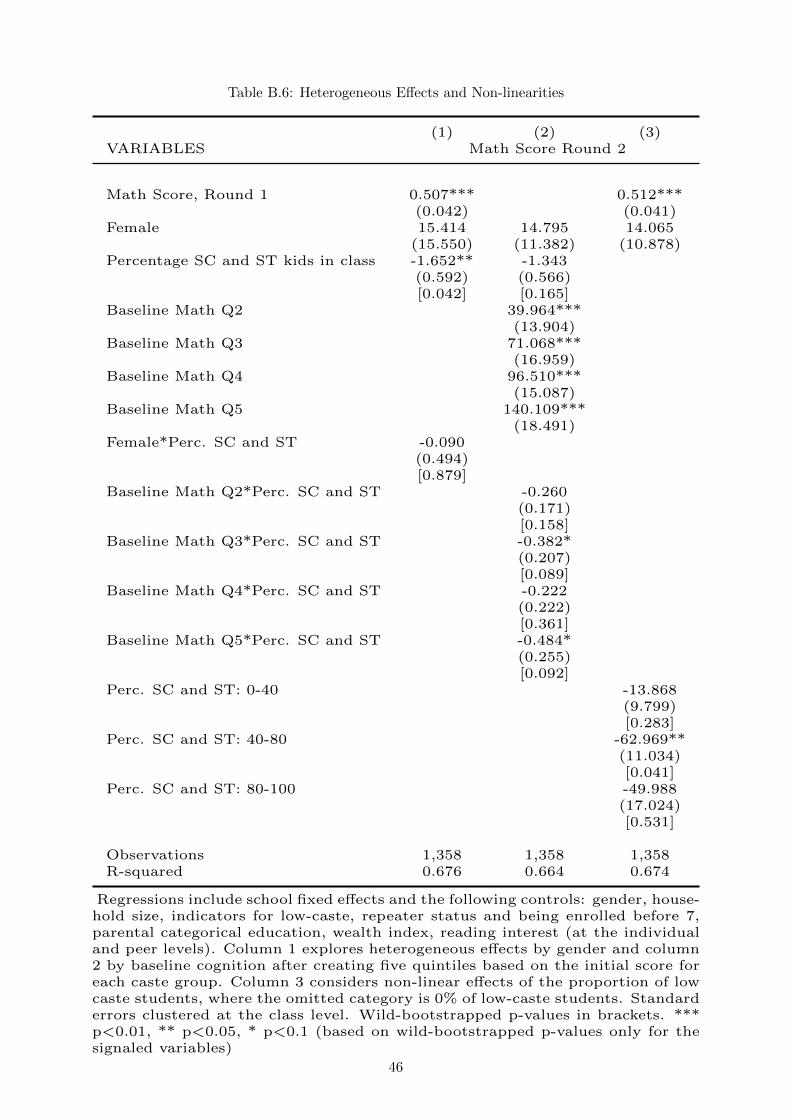
Table B.6: Heterogeneous E↵ects and Non-linearities
(1) (2) (3)
VARIABLES Math Score Round 2
Math Score, Round 1 0.507*** 0.512***
(0.042) (0.041)
Female 15.414 14.795 14.065
(15.550) (11.382) (10.878)
Percentage SC and ST kids in class -1.652** -1.343
(0.592) (0.566)
[0.042] [0.165]
Baseline Math Q2 39.964***
(13.904)
Baseline Math Q3 71.068***
(16.959)
Baseline Math Q4 96.510***
(15.087)
Baseline Math Q5 140.109***
(18.491)
Female*Perc. SC and ST -0.090
(0.494)
[0.879]
Baseline Math Q2*Perc. SC and ST -0.260
(0.171)
[0.158]
Baseline Math Q3*Perc. SC and ST -0.382*
(0.207)
[0.089]
Baseline Math Q4*Perc. SC and ST -0.222
(0.222)
[0.361]
Baseline Math Q5*Perc. SC and ST -0.484*
(0.255)
[0.092]
Perc. SC and ST: 0-40 -13.868
(9.799)
[0.283]
Perc. SC and ST: 40-80 -62.969**
(11.034)
[0.041]
Perc. SC and ST: 80-100 -49.988
(17.024)
[0.531]
Observations 1,358 1,358 1,358
R-squared 0.676 0.664 0.674
Regressions include school fixed e↵ects and the following controls: gender, house-
hold size, indicators for low-caste, repeater status and being enrolled before 7,
parental categorical education, wealth index, reading interest (at the individual
and peer levels). Column 1 explores heterogeneous e↵ects by gender and column
2 by baseline cognition after creating five quintiles based on the initial score for
each caste group. Column 3 considers non-linear e↵ects of the proportion of low
caste students, where the omitted category is 0% of low-caste students. Standard
errors clustered at the class level. Wild-bootstrapped p-values in brackets. ***
p<0.01, ** p<0.05, * p<0.1 (based on wild-bootstrapped p-values only for the
signaled variables)
46

Table B.7: Robustness: Alternative Estimating Sample and Attrition
(1) (2) (3)Math Score Attrited Attrited
VARIABLES Round 2
Percentage Low Caste Classmates -2.335*** -0.000 -0.000(0.410) (0.001) (0.001)[0.002] [0.824] [0.839]
Observations 835 1,921 1,819R-squared 0.611 0.111 0.115
All regressions include school fixed e↵ects. Column 1 is the counterpartof column 1 in Table 3’s Panel B with more strict sample restrictions.Compared to column 2 (no individual controls), column 3 additionallycontrols for gender, caste, parental education, household size, indicatorsfor repeater status and having first enrolled before age 7, wealth indexand interest in reading. Standard errors clustered at the class level. Stan-dard errors clustered at the class level. Wild-bootstrapped p-values inbrackets. *** p<0.01, ** p<0.05, * p<0.1 (based on wild-bootstrappedp-values only for the signaled variables)
47

C Variables Description
In this appendix I provide further details on the construction of certain variables.
• Wealth Index is computed as the proportion of positive answers to the questions of whether
the household owns each of the following twelve items: bicycle; motorbike; television; electric
fan; chairs; tables; telephone; fridge; car; air conditioning; computer; internet.
• The health categories considered are: sight problems; hearing problems; headaches; fever;
stomach aches; other problems.
• Reading interest is the principal component of the following three items:
– I read for fun outside the school.
– I read things that I choose myself outside of school.
– I read to find out things that I want to learn outside of school.
• Parental interest in their child’s school performance is the principal component of the degree
of agreement27 to the following four items:
– My parents (or someone else at home) asks me what I am learning at school.
– I talk about my schoolwork with someone at home.
– My parents (or someone else at home) makes sure that I set time aside for my homework.
– Someone at home checks if I do my homework.
• Student working to please her teacher is the principal component of the following three items:
– I want to do well in class to please my teacher.
– I want to do well at school so that I can get praise from my teacher.
– I do good work at school because I want to be recognised by my teacher.
• Student working hard to have better opportunities and outcomes in the future is the principal
component of the following twelve items:
– I study to increase my job opportunities for a good type of work in the future.
– I am working hard in school to ensure that my future will be financially secure.
– Making an e↵ort in my studies is worth it because it will help me in the work I want to
do later on.
27There are four possible categories: strongly disagree, disagree, agree, strongly agree. This categorical division is commonto all attitudinal questions in the survey.
48

– I want to learn as much as I can in school to help me get good work in the future.
– I want to learn as much as I can in school to help me go on to college/university.
– I am working hard in school to help me gain admission to higher studies.
– Making an e↵ort in my studies now is worthwhile because it will help me in my studies
later on.
– Learning well in school will improve my work prospects and chances in the future.
– I am working hard in school to be able to get work in the future and support my family
in the future.
– I want to do well at school to help my brothers and sisters in the future.
– Success in examinations will determine how successful I am in later life.
– Since success in the future is uncertain there is little use in learning very much.
• Student working hard to improve as a person is the principal component of the following ten
items:
– Studying gives me a lot of personal satisfaction.
– I like studying because most of my subjects are really interesting.
– I spend a lot of time working on topics I am interested in.
– Keeping up with my studies helps to develop my character.
– Learning is an important personal experience.
– Learning in school teaches me to become self-disciplined.
– I want to do well in school to show myself that I can learn new things.
– I want to do well in my studies to show myself that I can learn di�cult school work.
– I work hard at school because I am interested in what I am learning.
– Learning in school develops me as a person.
• Student works as hard as possible at school is the principal component of the following
fourteen items:
– I am willing to do my best in class.
– I study hard for my tests in school.
– If I put in enough e↵ort I can succeed in my studies.
– When studying, I work as hard as possible.
– When studying, I keep working even if the material is di�cult.
49

– When studying, I try to do my best to acquire the knowledge and skills taught.
– Setbacks in learning do not discourage me.
– I am a hard worker in school.
– I am diligent in my studies.
– I am conscientious in my studies.
– When studying, I want to do as little work as possible.
– I want to do well in my studies, but only if the work is easy.
– If the exercises in lessons are di�cult I just don’t do them.
– I choose easy options in school so that I don’t have to work too hard.
• Student math interest are the principal components of the following twelve items:
– I look forward to my maths lessons.
– I am interested in the things I learn in maths.
– The things I learn in maths will be important to me in the future.
– When I do maths, I sometimes get totally absorbed.
– Because doing maths is fun, I wouldn’t want to give it up.
– Maths is important to me personally.
– Studying maths gives me a lot of personal satisfaction.
– I do extra work in maths topics that I like.
– I find maths really boring.
– Maths is an important part of the school programme.
– I would rather spend my time on subjects other than Maths.
– Learning maths is a waste of time.
• Teacher is open with questions is the principal component of the following three items:
– If I don’t understand something, I can ask my teacher to explain again until I do
understand.
– If I need help I can always ask my teacher.
– When I ask a question my teacher will be nice to me.
• Teacher congratulates students for doing a good job is the principal component of the fol-
lowing two items:
50

– At least once a week my teacher will tell me that I have done good work.
– If I do something well, my teacher will come to me and congratulate me.
• Teacher cares about whether the students understand the material is the principal component
of the following four items:
– Every time my teacher explains something, we are asked whether we understand.
– My teacher will always notice when I don’t understand a topic and then come and help
me.
– My teacher always knows what I am doing.
– My teacher will notice immediately if I am not concentrating and tell me to focus.
• Teacher cares about students is the principal component of the following two items:
– My teacher never listens if I have something to ask or say.
– If I raise my hand to share, my teacher will always want to know what I think about a
topic.
51