Caste, Employment, and Wages in India: How do …€¦ · · 2018-01-23A Model of Wage Rate...

The views expressed in this working paper are those of the author (s) andnot necessarily endorsed by or representative of Indian Institute of Dalit Studies or the co-sponsoring or supporting organizations

Copyright ©2013 Indian Institute of Dalit Studies. All rights reserved.

I N D I A N I N S T I T U T E O F D A L I T S T U D I E S

Devoted to Studies on Social Exclusion, Marginalised Groups and Inclusive Policies

IND IAN INST I TUTE OF DAL I T S TUD IESD-ll/l, Road No. 4, Andrews Ganj, New Delhi 110 049T: +91-11-26252082 [email protected]

WORKING PAPER SERIESVolume VII Number 04, 2013

Caste, Employment, and Wages in India: How do Employees from Different Social Groups Fare in India’s Labour Market?

VAN I K BOROOAH

N IDH I SADANA SABHARWAL

A J AYA KUMAR NA I K

INDIAN

INST

ITUTE OF DALIT

STU

DIES

INDIAN

INST

ITUTE OF DALIT

STU

DIES INDIAN

INST

ITUTE OF DALIT

STUDIES

1

C a s t e , Em p l o y m e n t , a n d W a g e s i n In d i a

C a s t e , Em p l o y m e n t , a n d W a g e s i n In d i a : How do Employees from Different Social G r o u p s Fa r e i n In d i a ’ s La b o u r M a r k e t ?

V a n i K . B o r o o a hNidhi Sadana Sabharwal

Aj a y a K u m a r Na i k

W o r k i n g P a p e rIndian Institute of Dalit Studies

Ne w De l h i2 0 1 3

2

In d i a n In s t i t u t e o f Da l i t St u d i e sVolume VII, Number 04

3


Fo r e w o r d

The Indian Institute of Dalit Studies (IIDS) is among the pioneer Indian re-search organizations that focus exclusively on development concerns of mar-ginalized groups and socially excluded communities. Over the last 12 years, IIDS has carried out several studies on different aspects of social exclusion and discrimination of the historically marginalized social groups, such as Scheduled Castes, Scheduled Tribes and Religious Minorities in India and other parts of the sub-continent. The Working Paper Series disseminates empirical findings of on-going research and conceptual development on issues pertaining to the forms and nature of social exclusion and discrimination. Some of our papers also critically examine inclusive policies for the marginalized social groups.

The working paper on ‘Caste, Employment, and Wages in India: How do Em-ployees from Different Social Groups Fare in India’s Labour Market?’ attempts to quantify the effects of reserving jobs in India for people from the Sched-uled Castes (SC) and Scheduled Tribes (ST). The findings of the study explain that the two effects of positive discrimination in the public sector and negative discrimination in the private sector are ‘self-cancelling’. However, there was considerable discrimination between men from these groups in respect of re-muneration from regular salaried and wage employment. The paper suggests that the solution of identity based discrimination is to view education not just as imparting skills but also teaching norms of behaviour.

We hope the working paper will be of great help to academics, students, activ-ists, civil society organisations and policymakers.

Nidhi S. Sabharwal

Director

4


5


C o n t e n t s

Abstract 7

1. Introduction 8

2. Economic Status, Education and Community 10

3. A Multinomial Logit Model of Economic Status Outcomes 12

4. A Model of Wage Rate Determination 21

5. Conclusions 25

References 40

6


7


C a s t e , Em p l o y m e n t , a n d W a g e s i n In d i a : How do Employees from Different Social G r o u p s Fa r e i n In d i a ’ s La b o u r M a r k e t ?

V a n i K . B o r o o a h *Nidhi Sadana Sabharwal**

Aj a y K u m a r Na i k * * *

Abstract

This paper attempts to quantify the effects of reserving jobs in India for persons from the Scheduled Castes (SC) and Scheduled Tribes (ST). A major conclusion of the analysis was that there was no discrimination against SC, vis-à-vis High Caste Hindu (HCH) men in terms of their presence among those in regular salaried and wage employment (RSWE). As our results show, the two effects of positive discrimination in the public sector and negative discrimination in the private sector are self-cancelling. However, there was considerable discrimination between men from these groups in respect of remuneration from RSWE: 38% of the wage difference in RSWE was could not be explained by differences in labour market attributes.

* Vani K. Borooah, Professor of Economics, School of Economics, University of Ulster, UK. Email: [email protected]

** Nidhi Sadana Sabharwal, Director, Indian Institute of Dalit Studies Email: [email protected]

*** Ajay Kumar Naik, Associate Fellow, Indian Institute of Dalit Studies Email: [email protected]

8


1. Introduction

An important concern of public policy in India is to ensure that all persons, regardless of caste or religion, are treated fairly in the jobs market. There are two aspects to this concern. The first is whether differences in remuneration between persons fully reflect their difference in productivities or whether these differences might, wholly or in part, be due to ‘earning discrimination’. Oaxaca (1983) developed a methodology for answering this question and this has subsequently been applied to a variety of labour market situations by inter alia Reimers (1983), Neumark (1988), Oaxaca and Ransom (1994), Borooah et. al. (1995), and Harkness (1996). The second issue is concerns the different likelihoods that persons, from different social groups, will ceteris paribus attain different degrees of occupational success. The issue here is whether these differences in likelihoods are justified by differences in worker distribution or whether they are, wholly or in part, due to ‘occupational discrimination’. Smith and Strauss (1975), MacPherson and Hirsch (1995), Borooah (2001) are examples of such studies. This paper is concerned with the both issues – ‘earnings discrimination’ and ‘occupational discrimination’ – in the context of the Indian labour market.

In response to the burden of social stigma and economic backwardness borne by persons belonging to some of India’s castes, the Constitution of India allows for special provisions for members of these castes. Articles 341 and 342 include a list of castes and tribes entitled to such provisions and all those groups included in this list – and subsequent modifications to this list – are referred to as, respectively, “Scheduled Castes” (SC) and “Scheduled Tribes” (ST)1.

These special provisions have taken two main forms. The first is action against adverse discrimination towards persons from the SC and the ST. The second is compensatory discrimination in favour of persons from the SC and the ST. Compensatory discrimination has taken the form of guaranteeing seats in national and state legislatures and in village panchayats, places in educational institutions, and the reservation of a certain proportion of government jobs for the SC and the ST.

In the mind of the Indian public, however, it is jobs reservation that is seen

9


as the most important of the public concessions towards the SC and the ST and it is the one which arouses the strongest of passions.2 On the one hand, there is the demand to extend reservation to persons who are not from the SC or the ST but who, nevertheless, belong to economic and socially backward groups - the ‘other backward classes’ (OBC)3. On the other hand, there is the demand from the SC and the ST to extend reservation to private sector jobs4.

Given the fact that issues relating to occupational discrimination and unfair treatment of people belonging to certain castes and religions dominate public debate and discourse in India, it is surprising how little academic research there is on this subject (see, however, Dhesi and Singh, 1984; Esteve-Bolart, 2004; Borooah et. al., 2007; Thorat and Attewell, 2007; Ito, 2009). Are certain groups treated ‘unfairly’ treated in the jobs market in India? Unfairly treated with respect to access and/or with respect to wage rates? And, if they are indeed treated unfairly, is it possible to quantify the extent of unfair treatment?

This paper attempts to answer these questions using unit record data from the latest available round (68th: June 2011-June 2012) of the National Sample Survey (NSS) Employment Unemployment Survey. The NSS employment and unemployment data give the distribution of its respondents - who are distinguished by various characteristics, including their caste, religion, and educational levels - between different categories of economic status. Of these categories, the three which are the most important are: self-employed; regular salaried or wage employees; and casual wage employees.

Using these data, we focused on prime-age (22-45 years of age) males and estimated, using the methods of multinomial logit, the probabilities of men being in these categories of employment, after controlling for their caste/religion5 and their employment-related attributes.6 These estimates were then used, using the methodology detailed below, to decompose the observed difference between the castes in their proportions in the different categories of economic status into an ‘attributes’ and a ‘discrimination’ effect.

The NSS data also provided information on the wages/day earned by the employed respondents in their jobs. Using these data, we estimated wage data equations with a view to seeing whether ceteris paribus the caste (and religion) of the respondents played a role in determining these differences

10


or whether these differences were entirely the product of inter-respondent differences in employment-related attributes.

2. Economic Status, Education and Community

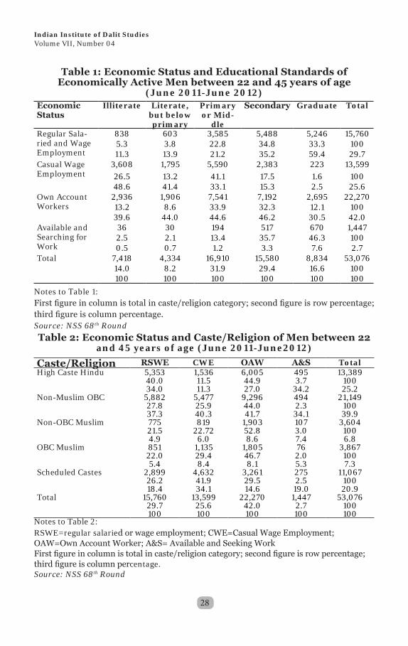
Table 1 shows, on the basis of data for the 68th round of the NSS (June 2011-June 2012), the distribution of 53,076 men, between the ages of 22 and 45 years (“prime-age” males), and living in the 16 major states of India and the Union Territories of Delhi and Chandigarh, by their educational standard, between the following categories of economic status7:

1. Regular Salaried and Wage Employment (RSWE)

1. Casual Wage Employment (CWE)

3. Own account employment (OAE)

4. Seeking and/or available for work (S&A)

Of these four categories, the first three were the main categories of economic status for prime-age men: 15,760 of the 53,076 men (30%) were in RSWE; 13,599 men (26% of the total) were in CWE; and 22,270 men (42% of the total) were in OAE. Only 1,447 men (3% of the total) were seeking and available for work.

Being in CWE or in OAE was largely the preserve of poorly educated men while those in RSWE were largely drawn from the ranks of the better educated: of the 13,599 men who were in CWE, 81% had an education standard less than secondary school and 27% were illiterate; of the 22,270 men in OAE, 56% had an education standard less than secondary school and 13% were illiterate; on the other hand, of the 15,760 men who were in RSWE, 68% were educated to secondary (or above) and 33% were graduates (or above).

This study implicitly assumes that becoming a regular salaried or wage worker was the most desirable outcome for prime-aged men and, compared to that, self-employment or casual wage worker were inferior outcomes. One can cite many justifications for this assumption. First, as referred to already, the Prime Minister of India has set up a high-powered committee to look at minority employment and, in particular, to examine why Muslims comprise only a fraction of India’s workforce. Second, this assumption is also consistent

11


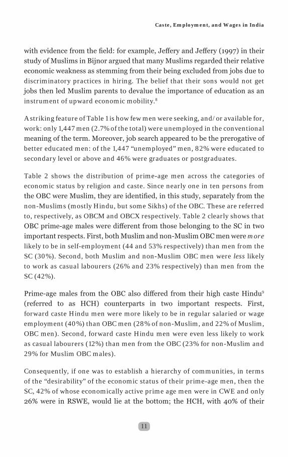
with evidence from the field: for example, Jeffery and Jeffery (1997) in their study of Muslims in Bijnor argued that many Muslims regarded their relative economic weakness as stemming from their being excluded from jobs due to discriminatory practices in hiring. The belief that their sons would not get jobs then led Muslim parents to devalue the importance of education as an instrument of upward economic mobility.8

A striking feature of Table 1 is how few men were seeking, and/or available for, work: only 1,447 men (2.7% of the total) were unemployed in the conventional meaning of the term. Moreover, job search appeared to be the prerogative of better educated men: of the 1,447 “unemployed” men, 82% were educated to secondary level or above and 46% were graduates or postgraduates.

Table 2 shows the distribution of prime-age men across the categories of economic status by religion and caste. Since nearly one in ten persons from the OBC were Muslim, they are identified, in this study, separately from the non-Muslims (mostly Hindu, but some Sikhs) of the OBC. These are referred to, respectively, as OBCM and OBCX respectively. Table 2 clearly shows that OBC prime-age males were different from those belonging to the SC in two important respects. First, both Muslim and non-Muslim OBC men were morelikely to be in self-employment (44 and 53% respectively) than men from the SC (30%). Second, both Muslim and non-Muslim OBC men were less likely to work as casual labourers (26% and 23% respectively) than men from the SC (42%).

Prime-age males from the OBC also differed from their high caste Hindu9

(referred to as HCH) counterparts in two important respects. First, forward caste Hindu men were more likely to be in regular salaried or wage employment (40%) than OBC men (28% of non-Muslim, and 22% of Muslim, OBC men). Second, forward caste Hindu men were even less likely to work as casual labourers (12%) than men from the OBC (23% for non-Muslim and 29% for Muslim OBC males).

Consequently, if one was to establish a hierarchy of communities, in terms of the “desirability” of the economic status of their prime-age men, then the SC, 42% of whose economically active prime age men were in CWE and only 26% were in RSWE, would lie at the bottom; the HCH, with 40% of their

12


economically active men in RSWE, and only 12% of their men working as casual labourers, would be at the top; and sandwiched between them would be the OBCX and OBCM (non-Muslim and Muslim Other Backward Classes).

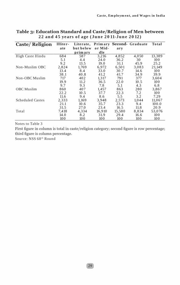
Lastly, Table 3 shows the education standards of prime-age men from the different communities. Economically active SC men, and their counterparts from OBC Muslims from the OBC, had the lowest level of educational achievement with more than one in five of them being illiterate. The best educated prime aged economically active men were from the HCH, only 5% of whom were illiterate and 30% of whom were graduates.

3. A Multinomial Logit Model of Economic Status Outcomes

The multinomial logit model has been used to analyse occupational outcomes by inter alia: Schmidt and Strauss (1975); Borooah (2001). The basic question that such a model seeks to answer is: what is the probability that a person with a particular set of characteristics, will be found in a specific category of economic status (hereafter, simply ‘status’)? These answers obtained by estimating the multinomial logit equation where the dependent variable Yi

took the values, 1, 2, or 3 depending upon whether person i is a regular salaried or wage worker; a casual wage worker ; or was self-employed (own-account worker).10 In essence, with self-employment (Yi =3) as the base category, the model consisted of two equations (Yi =1 and Yi =2) each of which took the following form:

Pr( )log (landholding, social group, education, state) + errorPr( 3)

i

i

Y j fY

== =

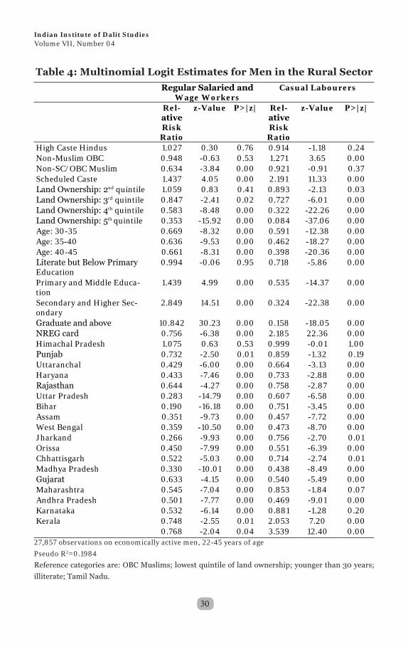
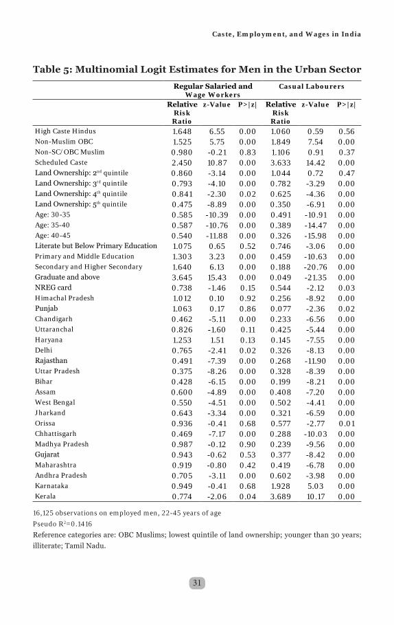
Tables 4 and 5 show estimates from the multinomial logit model estimated for, respectively, 28,532 prime-age men in the rural sector, and 16,719 prime-age men in the urban sector, who were in non-family employment, that is in one of the following (mutually exclusive) categories of economic status: regular salaried or wage employment (RSWE); casual wage employment (CWE); and own account employment (OAE). Hereafter, these employed (as employees or as self-employed) prime aged men are referred to as simply “men”. Excluded from the analysis were: 1,157 men who were employers, 8,262 men who were unpaid family workers, and the 1,447 men who were available for and seeking

work. The coefficient estimates are to be interpreted as the change in the log

13


risk-ratios,Pr( )logPr( 3)

i

i

Y jY

= =

, consequent upon a unit change in the value of the

associated variable.

Positive coefficients in Tables 4 and 5 imply that the ratio increases and negative coefficients imply that it decreases11. Because the community, the education standard, the age and the state categories in addition to being mutually exhaustive, were also collectively exhaustive, one of each category had to be omitted from the equation in order to avoid multicollinearity in the presence of the intercept term. These omitted categories were the reference categories: OBC Muslims, “illiteracy”, men under the age of 30 years, and Tamil Nadu were the reference categories for, respectively, social group, education, age, and state. The variables shown in Tables 4 and 5 are binary variables, taking the value 1 if a man belonged to that category and zero if he did not.

A New Methodology for Measuring Discrimination

The basic question that the multinomial logit model of income distribution sought to answer was: ceteris paribus what is the probability that a male, with a particular set of characteristics, will be found in a specific status: RSWE, CWE, or OAE? However, as observed earlier, the signs of the coefficient estimates associated with a variable - which, consequent upon a unit change in the value of the variable, reflect the directions of change in the risk-ratios - do not predict the directions of change in the probabilities of the outcomes.

Consequently, in order to answer these questions, we used the method of “predictive margins” to evaluate the following counterfactual scenarios:

1. We first treat all the men in the sample as high caste Hindus (HCH), with all other non-caste characteristics unchanged. In operational terms, ceteris paribus FCHi=1,OBCXi=0, MSXi=0, SCi=0, and OBCMi=0,i=1…N. where: OBCX refers to non-Muslim OBCs. Suppose that, under this scenario, HCH

jp is the average probability of a man belonging to status category j, j=0, 1, 2.

2. Next, we treat all the men in the sample as non-Muslims from the OBC,

14


with all other non-caste characteristics unchanged. In operational terms, ceteris paribus HCHi=0, OBCXi =1, MSXi=0, OBCMi=1, SCi=0, i=1…N. Suppose that, under this scenario, OBCX

jp is the average probability of a man belonging to status category j, j=1..4.

3. Next, we treat all the men in the sample as non-SC/OBC Muslims, with all other non-caste characteristics unchanged. In operational terms, ceteris paribus HCHi=0, OBCXi =0, MSXi=1, OBCMi=1, SCi=0, i=1…N. Suppose that, under this scenario, MSX


4. Next, we treat all the men in the sample as OBC Muslims, with all other non-caste characteristics unchanged. In operational terms, ceteris paribus HCHi=0, OBCXi =0, MSXi=0, OBCMi=1, SCi=0, i=1…N. Suppose that, under this scenario, OBCM


5. Lastly, we treat all the men in the sample as from the SC, with all other non-caste characteristics unchanged. In operational terms, ceteris paribusHCHi=0, OBCXi =0, MSXi=1, OBCMi=0, SCi=1, i=1…N. Suppose that, under this scenario, SC


The differences between the adjusted proportions, , , , , and HCH OBCX MSX OBCM SCj j j j jp p p p p

are entirely the result of different sets of coefficients (HCH, OBCX, MSX, OBCM, and SC) being applied to a given set of attributes. These differences may, therefore, be attributed to the unequal treatment of men who, except for their caste/religion, are identical in every respect. However, the sample proportions of men from the different caste groups – denoted,

, , , , HCH OBCX MSX OBCM SCj j j j jq q q q and q - will, in general, be different from the

adjusted proportions. This reflects the fact that men from the different social groups differ not just with respect to their caste/religious backgrounds but also with respect to their attributes. Then the overall disparity faced by (say) SC, relative to HCH, men, with respect to a “desirable” status category j (for example, RSWE), is measured by the disparity coefficient, 1- SC

jµ where:

, where: 0 1 SCjSC SC

j jHCHj

qq

µ µ= ≤ ≤ (1)

There is no disparity between males from the SC, relative to their HCH

15


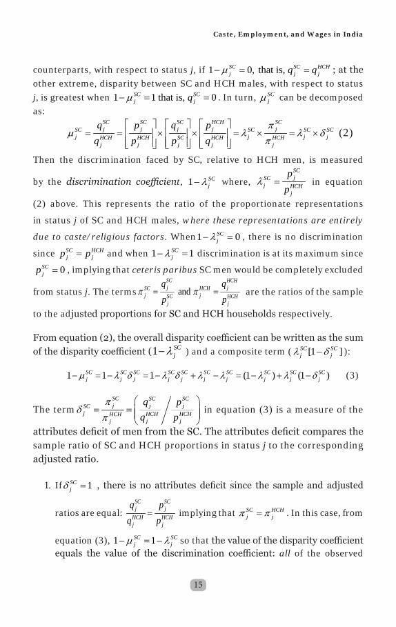
counterparts, with respect to status j, if 1 0, that is, SC SC HCHj j jq qµ− = = ; at the

other extreme, disparity between SC and HCH males, with respect to status j, is greatest when 1 1 that is, 0SC SC

j jqµ− = = . In turn, SCjµ can be decomposed

as: SC SC SC HCH SCj j j j jSC SC SC SC

j j j jHCH HCH SC HCH HCHj j j j j

q p q pq p p q

πµ λ λ δ

π

= = × × = × = ×

(2)

Then the discrimination faced by SC, relative to HCH men, is measured

by the discrimination coefficient, 1 SCjλ− where,

SCjSC

j HCHj

pp

λ = in equation

(2) above. This represents the ratio of the proportionate representations

in status j of SC and HCH males, where these representations are entirely

due to caste/religious factors. When1 0SCjλ− = , there is no discrimination

since SC HCHj jp p= and when 1 1SC

jλ− = discrimination is at its maximum since

0SCjp = , implying that ceteris paribus SC men would be completely excluded

from status j. The terms and SC HCHj jSC HCH

j jSC HCHj j

q qp p

π π= = are the ratios of the sample

to the adjusted proportions for SC and HCH households respectively.

From equation (2), the overall disparity coefficient can be written as the sum of the disparity coefficient (1 SC

jλ− ) and a composite term ( [1 ]SC SCj jλ δ− ):

1 1 1 (1 ) (1 )SC SC SC SC SC SC SC SC SC SCj j j j j j j j j jµ λ δ λ δ λ λ λ λ δ− = − = − + − = − + − (3)

The termSC SC SCj j jSC

j HCH HCHHCHj jj

q pq p

πδ

π

= =

in equation (3) is a measure of the

attributes deficit of men from the SC. The attributes deficit compares the sample ratio of SC and HCH proportions in status j to the corresponding adjusted ratio.

1. If 1SCjδ = , there is no attributes deficit since the sample and adjusted

ratios are equal: SC SCj j

HCH HCHj j

q pq p

= implying that SC HCHj jπ π= . In this case, from

equation (3), 1 1SC SCj jµ λ− = − so that the value of the disparity coefficient

equals the value of the discrimination coefficient: all of the observed

16


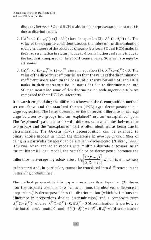
disparity between SC and HCH males in their representation in status j is due to discrimination.

2. If 1SCjδ < , (1 ) (1 )SC SC

j jµ λ− > − since, in equation (3), (1 ) 0SC SCj jλ δ− > . The

value of the disparity coefficient exceeds the value of the discrimination coefficient: some of the observed disparity between SC and HCH males in their representation in status j is due to discrimination and some is due to the fact that, compared to their HCH counterparts, SC men have inferiorattributes.

3. If 1SCjδ > , (1 ) (1 )SC SC

j jµ λ− < − since, in equation (3), (1 ) 0SC SCj jλ δ− < . The

value of the disparity coefficient is less than the value of the discrimination coefficient: more than all the observed disparity between SC and HCH males in their representation in status j is due to discrimination and SC men neutralise some of this discrimination with superior attributes compared to their HCH counterparts.

It is worth emphasising the differences between the decomposition method set out above and the standard Oaxaca (1973) type decomposition in a wage regression. The latter decomposes the observed difference in average wage between two groups into an “explained” and an “unexplained” part. The “explained” part has to do with differences in attributes between the two groups and the “unexplained” part is often identified as being due to discrimination. The Oaxaca (1973) decomposition can be extended to binary choice models in which the difference in average probabilities of being in a particular category can be similarly decomposed (Nielsen, 1998). However, when applied to models with multiple discrete outcomes, as in the multinomial logit model, the variable to be decomposed becomes the

difference in average log odds-ratios, Pr( )logPr( 3)

i

i

Y jY

= =

,which is not so easy

to interpret and, in particular, cannot be translated into differences in the underlying probabilities.

The method proposed in this paper overcomes this. Equation (3) shows how the disparity coefficient (which is 1 minus the observed difference in proportions) is decomposed into the discrimination (which is 1 minus the difference in proportions due to discrimination) and a composite term

(1 )SC SCj jλ δ− where: (1 ) 0, if 0SC SC SC

j j jλ δ λ− = = (discrimination is perfect, so attributes don’t matter) and (1 ) 1 , if 1SC SC SC SC

j j j jλ δ δ λ− = − = (discrimination

17


is absent, so observed differences depend only on attribute differences). In between these extremes, (1 ) / 1 0SC SC SC SC

j j j jλ δ λ δ∂ − ∂ = − > so attribute differences become more (less) important in explaining observed differences as discrimination becomes weaker (stronger).

Measuring Discrimination

Tables 6 and 7 show values of the disparity and discrimination coefficients, with respect to regular and salaried and wage employment, for men in the rural and urban sectors, respectively, using high caste Hindus as the comparator. Tables 6 and 7 show that the observed proportion of high caste Hindu (HCH) men in RSWE was 25.5% in the rural sector and 46.3% in the urban sector; the observed proportion of non-Muslim OBC (OBCX) men in RSWE was 18.1% in the rural sector and 35.9% in the urban sector; the observed proportion of non-OBC Muslim (MSX) men in RSWE was 13.1% in the rural sector and 26.0% in the urban sector; the observed proportion of Muslim OBC (OBCM) men in RSWE was 15.1% in the rural sector and 24.8% in the urban sector; and the observed proportion of Scheduled Caste (SC) men in RSWE was 17.2% in the rural sector and 37.8% in the urban sector.

1. If everyone in the sample (the OBCX, MSX, OBCM, and SC men) was treated as HCH (in effect, had their attributes evaluated at HCH coefficients), the proportion of men in RSWE would fall from 26.2% to 21.1% in the rural sector and from 48.7% to 43.3% in the urban sector. These falls reflect that the fact that when the entire sample of men was being treated as HCH, it had a lower quality of attributes than the HCH sub-sample. Consequently the adjusted proportions (21.1% and 41.5%) were lower than the observed proportions of HCH men (25.5% and 43.3%) in RSWE.

2. If everyone in the sample (the HCH, the MSX, OBCM, and SC men) was treated as OBCX (in effect, had their attributes evaluated at OBCX coefficients), the proportion of men in RSWE would remain unchanged at 18.5% in the rural sector and rise from 36.9% to 38.3% in the urban sector. These small changes reflect the fact that the attributes of the men in the sample, considered in its entirety, was broadly similar to the attributes of the OBCX sub-sample of men.

3. If everyone in the sample (the HCH, OBCX, the OBCM, and the SC men)

18


was treated as MSX (in effect, had their attributes evaluated at MSX coefficients), the proportion of men in RSWE would rise from 13.4% to 16% in the rural sector and rise from 26.8% to 31.6% in the urban sector. These increases reflect the fact that when the entire sample of men was being treated as MSX, it had a higher quality of attributes than the MSX sub-sample. Consequently the adjusted proportions (16% and 31.6%) were higher than the observed proportions of MSX men (13.4% and 26.8%) in RSWE.

4. If everyone in the sample (the HCH, OBCX, MSX, and SC men) was treated as OBCM (in effect, had their attributes evaluated at OBCM coefficients), the proportion of men in RSWE would rise from 15.4% to 19.3% in the rural sector and from 25.2% to 31.6% in the urban sector. These increases reflect the fact that when the entire sample of men was being treated as OBCM, it had a higher quality of attributes than the OBCM sub-sample. Consequently the adjusted proportions (19.3% and 31.6%) were higher than the observed proportions of OBCM men (15.4% and 25.2%) in RSWE.

5. Lastly, if everyone in the sample (the HCH, OBCX, MSX, and OBCM men) was treated as SC (in effect, had their attributes evaluated at SC coefficients), the proportion of men in RSWE would rise from 17.6% to 21.3% in the rural sector and from 39.1% to 44.1% in the urban sector. These increases reflect the fact that when the entire sample of men was being treated as SC, it had a higher quality of attributes than the SC sub-sample. Consequently the adjusted proportions (21.3% and 44.1%) were higher than the observed proportions of SC men (17.6% and 39.1%) in RSWE.

A feature of the results shown in Tables 5 and 6 is that when the chances of the men in the sample being in RSWE were evaluated using, in turn, the coefficients of each group, the adjusted proportions in RSWE were highest when the HCH coefficients were used. The implication of this is that Hindu coefficients were most favourable for being in RSWE or, in other words, the same group of people (that is, all the men in the sample) would have had a higher chance of being in RSWE had they all been HCH compared to all being OBCX, or MSX, or OBCM. As argued above, 1 minus the ratio of the HCH and the OBCX (or MSX or OBCM) adjusted proportions (1 /OBCX HCH

j jp p− ) is

19


the value of the discrimination coefficient against OBCX (or MSX or OBCM), vis-à-vis HCH, men and this, as Tables 6 and 7 show, was always positive. In terms of RSWE, men from the OBCX, the MSX, and the OBCM were discriminated against vis-à-vis HCH men.

The exception to this general observation arose when all the men in the sample were treated as though they were from the SC. In this case, the adjusted proportions were the same – both for the rural and urban sectors – as those which resulted from treating all the men as though they were HCH. In other words, it made no difference to the chances of the men in the sample being in RSWE whether their attributes were evaluated using HCH or SC coefficients; to put it differently, the results shown in Tables 6 and 7 imply that there was no discrimination against SC, vis-à-vis HCH, men!

The answer to this counter-intuitive result lies in the reservation of jobs for the SC instituted, as noted above, under the aegis of the Indian constitution. A major reason for jobs reservation was to combat discrimination against persons from the SC who, along with persons from the Scheduled Tribes, are arguably the most down trodden of India’s population. Jobs reservation cannot alter the employment-related attributes of the SC but, given those attributes, it can raise the proportion of persons from the SC who secure RSWE by shifting the coefficients of the employment equations in favour of persons from this group. In respect, jobs reservation for the SC has succeeded in neutralising the discrimination that they undeniably face from other sections of Indian society. For SC men who, for reasons of discrimination, are turned down for RSWE in favour of a HCH man in the private sector, where jobs reservation does not apply, positive discrimination ensures that there are HCH men who are turned down in favour of SC men in the public sector where jobs reservation does apply. As our results show, the two effects are self-cancelling: positive discrimination its favour of SC men neutralises its negative counterpart against SC men.

So, given their attributes and the advantage of jobs reservation (as reflected in the SC coefficients), SC men achieve a RSWE representation of 17.6% in rural areas and 39.1% in urban areas. If everyone was treated as a SC male, RSWE representation would rise to 21.3% in rural areas and 44.1% in urban areas – the superior attributes of the men in the sample in its entirety,

20


relative to men in the SC sub-sample, would combine with jobs reservation(as reflected in the SC coefficients) to yield the higher proportions in RSWE.

These observations then raise the counterfactual question of what the representation of SC men in RSWE would have been had they not been protected by jobs reservation? In order to see how effective jobs reservation was in raising the proportions of SC men in RSWE we consider what these proportions would have been if the attributes of these men had been evaluated using the coefficients of employment-deficit groups who did not benefit from jobs reservation: OBC and non-OBC Muslims. This was implemented by estimating the multinomial logit equations, shown in Tables 4 and 5, on the Muslim subsample (MSX+OBCM) only and then using these estimates to predict the proportion SC men in RSWE. Our results show that if SC men had been treated as Muslims, their proportion in RSWE in the rural sector would have fallen from the observed 17.6% to 16% and proportion in RSWE in the urban sector would have fallen from the observed 39.1% to 28.3%. So, on our estimates, jobs reservation added 1.6 percentage points to SC male representation in RSWE in the rural sector and added 10.8 percentage points to SC male representation in RSWE in the urban sector.

Jobs reservation is, of course, one way of raising SC representation in RSWE. Another way is to raise the educational levels of persons from the SC. For example, as Table 3 shows, 21% of SC, compared to 13% of non-Muslim OBC and 10% of non-OBC Muslim, men were illiterate. At the other end of the educational spectrum, only 9% of SC, compared to 13% of non-Muslim OBC and 11% of non-OBC Muslim, men were graduates. So, a natural question that rises is by how much would the RSWE representation of SC males improve if their educational levels rose to, say, that of non-OBC men?

Our calculations suggest that if men from the SC in the rural sector had had the education standards of rural sector non-Muslim men from the OBC, their proportion in rural RSWE would have been 22% instead of the observed 17.6% and their proportion in urban RSWE would have been 42.1% instead of the observed 39.1%: rises of 4.4 and 3 points which could be ascribed to the rise in the education standard of men from the SC to the standard of non-Muslims from the OBC.

21


Access to RSWE is one aspect of labour market welfare and, as we have argued, jobs reservation has succeeded in delivering to SC men a share in urban RSWE that is nearly 11 points more than what they might have expected in its absence. However, another aspect of labour market welfare is the quality of RSWE. Although this quality has many dimensions, the wage rate obtained in RSWE is, arguably, a good encapsulation of these. The next section turns to a discussion of issues relating to wages.

4 . A M o d e l o f W a g e R a t e De t e r m i n a t i o n

The NSS gives details of a person’s current weekly status in terms of whether in the course of a reference week a person was: in RSWE; in casual wage employment; self-employment; unemployed. The NSS also reports the intensity of work in terms of whether a person, if he was not unemployed, worked a full day (value 1) or a half day (value 0.5). The maximum and minimum number of (full) days an employed person could work was, therefore, 7 and 0.5, respectively.12 The NSS also reports on the total wages received every person who was employed during that week; dividing wages by the number of days worked then yields the daily wage rate. Hereafter, this is referred to as the wage rate.

Table 8 shows that the wage rate for HCH men in rural and urban RSWE was, respectively, 32% and 64% above the corresponding SC wage rate: HCH men earned Rs. 391 and Rs. 556 per day, while SC men earned Rs. 296 and Rs. 339 per day, in, respectively, rural and urban RSWE. The mark up of the RSWE wage rate over the wage rate for CWE was considerably higher for HCH, compared to SC, men: 2.4 and 2.8 for HCH men in the rural and urban sectors and 1.8 for SC men in both sectors. HCH males also earned 42% more in urban, compared to rural, RSWE while OBCM males earned only 2% more (Rs. 288 compared to Rs. 282) and OBCX males actually earned less in the urban, compared to the rural, sector (Rs. 361 versus Rs. 334).

Tables 9 and 10 show the results of estimating a wage equation, in which the dependent variable was the wage rate (as defined above) for, respectively, the sample of 15,902 men in rural India and the sample of 10,096 employee men in urban India. The rural and urban equations explained, respectively, 33.5% ( 2 0.335R = ) and 26.9% ( 2 0.269R = ) of the variation in wage rates among

22


men. The interpretation of the estimates in these tables is as follows. A male with all the “reference” characteristics (an OBC Muslim male in casual wage employment, below the age of 30, owning minimal or no land, illiterate, not holding a National Rural Employment Guarantee (NREG) card, and living in Tamil Nadu would earn Rs. 178 and Rs. 90 as daily wages in, respectively, the rural and urban sectors. For such a man, working in the rural sector in any other state of India (except Kerala, where he would earn Rs. 83 more) would reduce his wages for example, by Rs. 58 in Maharashtra and by Rs. 31 in Punjab. However, working in the urban sector, would raise his wage rate in several states: in Delhi by Rs. 189, in Haryana by Rs. 180, and in Kerala by Rs. 78.

By far, ceteris paribus the largest contributor to a higher wage rate was being a graduate or higher. Having this educational level would add Rs. 235 to the wage rate in rural areas and Rs. 400 to the wage rate in urban areas; in contrast, having a level of education between higher secondary and a diploma would add only Rs. 60 to the rural wage rate and Rs. 88 to the urban wage rate. The next biggest contributor was in being in regular, as opposed to casual, employment – this fact would add Rs. 72 to the rural wage rate and Rs. 59 to the urban wage rate. In rural areas, those who had a NREG card would earn Rs. 36 less in daily wages than those who did not have this card.

Not surprisingly, the wage rate increased with the wage of the employee: workers who were aged 40-45 earned more than workers aged 35-40, who earned more than workers aged 30-35 workers and who, in turn, earned more than the youngest (below 30 years) workers. In a similar fashion, the wage rate was higher for those who owned more assets by way of land: workers who were in the top quintile of land owners earned more than workers in the next quintile and so on.

Compared to rural areas, caste effects on the wage rate were significant in both rural and urban India but these were stronger in urban areas. With OBC Muslims as the reference group, ceteris paribus HCH males earned Rs. 72 more in daily wages than OBC Muslims in urban areas but only Rs. 6 more in rural areas; SC males earned Rs. 25 less in daily wages than OBC Muslims in urban areas but only Rs. 5 less in rural areas. A slightly surprising feature of the results is that ceteris paribus except for HCH males, men in all the groups

23


had a lower wage rate in the urban sector than for OBC men and, except for HCH and non-OBC Muslims, also had a lower wage rate in the rural sector than for OBC men. This can largely be explained by the high wage rate for OBC men in casual wage employment – as Table 8 shows, OBC Muslim men had the highest CWE wage rate in the rural sector (Rs. 196) and the CWE wage rate of OBC Muslim men in the urban sector (Rs. 198) was only slightly lower than that for non-OBC men (Rs. 201) and considerably higher than that for non-OBC Muslim (Rs. 164) and SC (Rs. 184) males. Excluding HCH males, of the total number of employees in the sample, 59% of were in CWE, with 41% in RSWE. In terms of the overall wage rate, therefore, this put OBC Muslim men at an advantage over men from all groups except HCH males.

The Decomposition of Wage Rates

In the previous analysis, a single regression was estimated over all the regardless of the group to which they belonged. The implicit assumption was that all the men from the different groups (HCH, OBCX, MSX, OBCM, SC) faced the same regression coefficients in the evaluation of their attributes and that the only coefficient that distinguished between them the caste/religion variable. Under this assumption, as discussed above, caste played a significant role in determining wage rates.

This assumption is relaxed by estimating separate equations between the two groups and allowing the coefficients to be different between them. This raises the following question: when we observe a difference in mean achievement between the groups how much is it due to a difference in attributes and how much is due to a difference in coefficients? So the first step is to ask what the HCH/SC difference (and the HCH/OBCX, the HCH/MSX, and the HCH/OBCM difference) would have been if both sets of attributes were evaluated at a common coefficient vector. This difference could then be entirely ascribed to a difference in attributes since coefficient differences would have been neutralised. Then the observed difference less the difference due to attributes is the residual or unexplained difference. It is this residual difference that can, subject to several caveats, be interpreted as due to discrimination.13

A recent formal exposition of the Blinder-Oaxaca (B-O) decomposition method (named after Blinder, 1973 and Oaxaca, 1973) for linear regression

24


models is to be found in Jann (2008).Suppose there are two groups, H and S with Y as an outcome variable such that E(YH)and E(YS)are the expectedvalues of the outcome variable for, respectively, groups H and S. Then:

SHkXY kkkk ,,' =+= εβ (4)

Where Y k is the vector of outcomes, X k is the matrix of observations, and ε k is the vector of error terms for persons in group k. Since, by assumption E(ε k )=0, we have:

* * * *

* * *

( ) ( ) ( ) ( )

( ) ( ) ( ) ( ) ( ) ( )

( ) ( )( ) ( )( )

H S H H S S

H H S S H H S S

H S H H S S

R E Y E Y E X E X

E X E X E X E X E X E X

E X X E X E X

U V

β β

β β β β β β

β β β β β

′ ′= − = −

′ ′ ′ ′ ′ ′= − + − + −

′ ′′= − + − + −

= + (5)

Equation (5) yields a two-fold decomposition in which the term *( )H SU E X X β′= − is the part of the outcome difference that can be explained by

the difference in attributes, and the term * *( )( ) ( )( )H H S SV E X E Xβ β β β′ ′= − + −

is the unexplained part. The latter is usually ascribed to discrimination. In general, the problem of defining β*, the non-discriminatory coefficient vector, is a big issue in the decomposition literature on discrimination. One possibility is to identify β* with the coefficients of one of the groups. Another is to regard it as the average of the two group coefficients (Reimers, 1983): * 0.5 0.5H Sβ β β= × + × . Yet another (Cotton, 1988) is to weight the coefficients by the size of the groups: *

H H S Sn nβ β β= × + × where nH and nS

are the proportions in groups H and S. The pair-wise decompositions in this paper were carried out by the pooling the observations for: HCH and SC men; HCH and OBCX men; HCH and MSX men; HCH and OBCM men. Separate pairwise decompositions were conducted by RSWE and CWE wage rates for the rural and urban sectors: (i) rural, RWSE; (ii) rural CWE; (iii) urban RWSE; (iv) urban CWE.

Tables 11-14 show the results from the decomposition analysis for RSWE in the urban sector.14 For example, Table 14 shows that that there was a difference of Rs. 231 between the HCH and SC male wage rates: Rs. 573 and Rs. 341, respectively. Of this difference, Rs. 144 (62%) was due to a difference in attributes between males from the two groups and Rs. 87 (38%) was the “unexplained” difference. Tables 12 and 13 show that for Muslim males (both

25


non-OBC and OBC), the contribution of the attributes difference was much higher – 71% for non-OBC Muslim and 77% for OBC Muslim males; lastly, Table 11 shows that the contribution of the attributes difference was smallest for 55%.

The above observations beg the question of what are the attributes that matter in explaining differences between the social groups in their male wage rates for RSWE in the urban sector. Table 15 shows the contributions that differences in the various attributes made to the overall attributes difference between of HCH males and males from the other groups in their urban RSWE wage rate. The largest contribution to the attribute difference between HCH males and males from the other groups was graduate level education. The difference in this attribute alone accounted for: 74% of the total attributes difference between HCH and non-Muslim OBC males (Rs. 75 of Rs. 106); 75% of the total attributes difference between HCH and non-OBC Muslim males (Rs. 117 of Rs. 157); 70% of the total attributes difference between HCH and OBC Muslim males (Rs. 162 of Rs. 232); and 88% of the total attribute difference between HCH and SC males (Rs. 127 of Rs. 144).

5. Conclusions

This paper attempted to quantify the effects of reserving jobs in India for persons from the SC and ST. A major conclusion of the analysis was that it made no difference to the chances of the men in the sample being in regular salaried or wage employment (RSWE) whether their attributes were evaluated using HCH or SC coefficients; to put it differently, the results showed that there was no discrimination against SC, vis-à-vis HCH, men in terms of their presence among those in RSWE!

The answer to this counter-intuitive result lies in the reservation of jobs for the SC instituted, as noted above, under the aegis of the Indian constitution. The goal of jobs reservation in India has been to bring about an improvement in the welfare of those who are, and have been for a long time, economically and socially depressed. A major reason for jobs reservation was to combat discrimination against persons from the SC who, along with persons from the Scheduled Tribes, are arguably the most down trodden of India’s population.

26


Jobs reservation cannot alter the employment-related attributes of the SC but, given those attributes, it can raise the proportion of persons from the SC who secure RSWE by shifting the coefficients of the employment equations in favour of persons from this group. In this respect, jobs reservation for the SC has succeeded in neutralising the discrimination that they undeniably face from other sections of Indian society. For SC men who, for reasons of discrimination, are turned down for RSWE in favour of a HCH man in the private sector - where jobs reservation does not apply - positive discrimination ensures that there are HCH men who are turned down in favour of SC men in the public sector where jobs reservation does apply. As our results show, the two effects are self-cancelling: positive discrimination its favour of SC men neutralises its negative counterpart against SC men. However in comparison to the other groups, Hindu coefficients were most favourable for being in RSWE or, in other words, ceteris paribus our sample of men would have had a higher chance of being in RSWE had they all been HCH compared to allbeing OBCX, or MSX, or OBCM. To put it differently, compared to HCH men, men from the OBCX, the MSX, and the OBCM were discriminated against in respect of RSWE.

Compared to an absence of discrimination, between men from the HCH and the SC, in respect of access to RSWE, there was considerable discrimination between men from these groups in respect of remuneration from RSWE. Of the difference of Rs. 231 between the HCH and SC male wage rates in RSWE (Rs. 573 and Rs. 341, respectively), 62% was due to a difference in attributesbetween males from the two groups and 38% was the result of unexplaineddifference. For Muslim males (both non-OBC and OBC), the contribution of the attributes difference was much higher – 71% for non-OBC Muslim and 77% for OBC Muslim males whereas, at 55%, the contribution of the attributes difference was smallest for OBC Hindu males.

In terms of the important attributes that influenced wage rates, the most important was graduate level education. The contribution of this attribute alone accounted for 70%-88% of the total attributes contribution to the RSWE wage rate difference between HCH and non-HCH males. If employees from the non-HCH groups could raise their performance in respect of degree level education to HCH levels then much of the difference in RSWE wage rates between them and HCH males due to attribute differences would disappear.

27


However, needless to say, differences in RSWE wages due to discrimination would continue.

The importance of education forces one to reflect on the schooling experience of Dalit and Muslim children. Thrown in as a minority group with children from the higher social groups they face discrimination, exclusion, and humiliation. Nambissan (2010) in her study of the experiences of Dalit children in schools in Jaipur district in the state of Rajasthan concluded that “social relations and the pedagogic processes fail to ensure full participation of Dalit children and they are subject to discriminatory and unequal treatment in relation to their peers” (p. 282). Ramachandran and Naorem (2013) call on policymakers in India to officially acknowledge the prevalence of exclusionary practices in schools and the urgent need to address them.

The role of social identity in shaping outcomes in work and education has been extensively discussed by Akerlof and Kranton (2010). They argued that the traditional economic model in which students, as rational decision makers, weighed the economic costs and benefits of schooling was flawed because it took no account of the constraints imposed by the social identities of the children. Using examples from the USA, they showed that the social burden of being Black or Hispanic led many children from such groups to underperform relative to their white peers even within the same school: consequently, relative to social pressures, the economic return to education in terms of more pleasant and better paid jobs could be a weak determinant of children’s efforts at school. The solution for such “identity-based” problems is to view schools not just as imparting skills but also teaching norms of behaviour and, by so doing, becoming a sanctuary from the dysfunctional world outside its walls.

28


Table 1: Economic Status and Educational Standards of Economically Active Men between 22 and 45 years of age

( J u n e 2 0 1 1 - J u n e 2 0 1 2 )Economic Status

Il l i t e r a t e Li t e r a t e , b u t b e l o w p r i m a r y

P r i m a r y o r M i d -

d l e

Secondary G r a d u a t e To t a l

Regular Sala-ried and Wage Employment

838 603 3,585 5,488 5,246 15,7605.3 3.8 22.8 34.8 33.3 10011.3 13.9 21.2 35.2 59.4 29.7

Casual Wage Employment

3,608 1,795 5,590 2,383 223 13,59926.5 13.2 41.1 17.5 1.6 10048.6 41.4 33.1 15.3 2.5 25.6

Own Account Workers

2,936 1,906 7,541 7,192 2,695 22,27013.2 8.6 33.9 32.3 12.1 10039.6 44.0 44.6 46.2 30.5 42.0

Available and Searching for Work

36 30 194 517 670 1,4472.5 2.1 13.4 35.7 46.3 1000.5 0.7 1.2 3.3 7.6 2.7

Total 7,418 4,334 16,910 15,580 8,834 53,07614.0 8.2 31.9 29.4 16.6 100100 100 100 100 100 100

Notes to Table 1:First figure in column is total in caste/religion category; second figure is row percentage; third figure is column percentage.Source: NSS 68th RoundTable 2: Economic Status and Caste/Religion of Men between 22

a n d 4 5 y e a r s o f a g e ( J u n e 2 0 1 1 - J u n e 2 0 1 2 )Caste/Religion RSWE C W E OAW A&S To t a lHigh Caste Hindu 5,353 1,536 6,005 495 13,389

40.0 11.5 44.9 3.7 10034.0 11.3 27.0 34.2 25.2

Non-Muslim OBC 5,882 5,477 9,296 494 21,14927.8 25.9 44.0 2.3 10037.3 40.3 41.7 34.1 39.9

Non-OBC Muslim 775 819 1,903 107 3,60421.5 22.72 52.8 3.0 1004.9 6.0 8.6 7.4 6.8

OBC Muslim 851 1,135 1,805 76 3,86722.0 29.4 46.7 2.0 1005.4 8.4 8.1 5.3 7.3

Scheduled Castes 2,899 4,632 3,261 275 11,06726.2 41.9 29.5 2.5 10018.4 34.1 14.6 19.0 20.9

Total 15,760 13,599 22,270 1,447 53,07629.7 25.6 42.0 2.7 100100 100 100 100 100

Notes to Table 2:RSWE=regular salaried or wage employment; CWE=Casual Wage Employment; OAW=Own Account Worker; A&S= Available and Seeking WorkFirst figure in column is total in caste/religion category; second figure is row percentage; third figure is column percentage.Source: NSS 68th Round

29


Table 3: Education Standard and Caste/Religion of Men between 2 2 a n d 4 5 y e a r s o f a g e ( J u n e 2 0 1 1 - J u n e 2 0 1 2 )

Caste/ Religion Il l i t e r -a t e

Li t e r a t e , b u t b e l o w p r i m a r y

P r i m a r y o r M i d -

d l e

Second-a r y

G r a d u a t e To t a l

High Caste Hindu 684 587 3,216 4,852 4,050 13,3895.1 4.4 24.0 36.2 30 1009.2 13.5 19.0 31.1 45.9 25.2

Non-Muslim OBC 2,824 1,769 6,972 6,501 3,083 21,14913.4 8.4 33.0 30.7 14.6 10038.1 40.8 41.2 41.7 34.9 39.9

Non-OBC Muslim 717 402 1,317 791 377 3,60419.9 11.2 36.5 22.0 10.5 1009.7 9.3 7.8 5.1 4.3 6.8

OBC Muslim 860 407 1,457 863 280 3,86722.2 10.5 37.7 22.3 7.2 10011.6 9.4 8.6 5.5 3.2 7.29

Scheduled Castes 2,333 1,169 3,948 2,573 1,044 11,06721.1 10.6 35.7 23.3 9.4 100.031.5 27.0 23.4 16.5 11.8 20.9

Total 7,418 4,334 16,910 15,580 8,834 53,07614.0 8.2 31.9 29.4 16.6 100100 100 100 100 100 100

Notes to Table 3First figure in column is total in caste/religion category; second figure is row percentage; third figure is column percentage.Source: NSS 68th Round

30


Table 4: Multinomial Logit Estimates for Men in the Rural SectorRegular Salaried and

W a g e W o r k e r sC a s u a l La b o u r e r s

R e l -ative R i s k R a t i o

z - V a l u e P > | z | R e l -ative R i s k R a t i o

z - V a l u e P > | z |

High Caste Hindus 1.027 0.30 0.76 0.914 -1.18 0.24Non-Muslim OBC 0.948 -0.63 0.53 1.271 3.65 0.00Non-SC/OBC Muslim 0.634 -3.84 0.00 0.921 -0.91 0.37Scheduled Caste 1.437 4.05 0.00 2.191 11.33 0.00Land Ownership: 2nd quintile 1.059 0.83 0.41 0.893 -2.13 0.03Land Ownership: 3rd quintile 0.847 -2.41 0.02 0.727 -6.01 0.00Land Ownership: 4th quintile 0.583 -8.48 0.00 0.322 -22.26 0.00Land Ownership: 5th quintile 0.353 -15.92 0.00 0.084 -37.06 0.00Age: 30-35 0.669 -8.32 0.00 0.591 -12.38 0.00Age: 35-40 0.636 -9.53 0.00 0.462 -18.27 0.00Age: 40-45 0.661 -8.31 0.00 0.398 -20.36 0.00Literate but Below Primary Education

0.994 -0.06 0.95 0.718 -5.86 0.00

Primary and Middle Educa-tion

1.439 4.99 0.00 0.535 -14.37 0.00

Secondary and Higher Sec-ondary

2.849 14.51 0.00 0.324 -22.38 0.00

Graduate and above 10.842 30.23 0.00 0.158 -18.05 0.00NREG card 0.756 -6.38 0.00 2.185 22.36 0.00Himachal Pradesh 1.075 0.63 0.53 0.999 -0.01 1.00Punjab 0.732 -2.50 0.01 0.859 -1.32 0.19Uttaranchal 0.429 -6.00 0.00 0.664 -3.13 0.00Haryana 0.433 -7.46 0.00 0.733 -2.88 0.00Rajasthan 0.644 -4.27 0.00 0.758 -2.87 0.00Uttar Pradesh 0.283 -14.79 0.00 0.607 -6.58 0.00Bihar 0.190 -16.18 0.00 0.751 -3.45 0.00Assam 0.351 -9.73 0.00 0.457 -7.72 0.00West Bengal 0.359 -10.50 0.00 0.473 -8.70 0.00Jharkand 0.266 -9.93 0.00 0.756 -2.70 0.01Orissa 0.450 -7.99 0.00 0.551 -6.39 0.00Chhattisgarh 0.522 -5.03 0.00 0.714 -2.74 0.01Madhya Pradesh 0.330 -10.01 0.00 0.438 -8.49 0.00Gujarat 0.633 -4.15 0.00 0.540 -5.49 0.00Maharashtra 0.545 -7.04 0.00 0.853 -1.84 0.07Andhra Pradesh 0.501 -7.77 0.00 0.469 -9.01 0.00Karnataka 0.532 -6.14 0.00 0.881 -1.28 0.20Kerala 0.748 -2.55 0.01 2.053 7.20 0.00

0.768 -2.04 0.04 3.539 12.40 0.0027,857 observations on economically active men, 22-45 years of agePseudo R2=0.1984Reference categories are: OBC Muslims; lowest quintile of land ownership; younger than 30 years; illiterate; Tamil Nadu.

31


Table 5: Multinomial Logit Estimates for Men in the Urban Sector

Regular Salaried and W a g e W o r k e r s

C a s u a l La b o u r e r s

Relative R i s k R a t i o

z - V a l u e P > | z | Relative R i s k R a t i o

z - V a l u e P > | z |

High Caste Hindus 1.648 6.55 0.00 1.060 0.59 0.56Non-Muslim OBC 1.525 5.75 0.00 1.849 7.54 0.00Non-SC/OBC Muslim 0.980 -0.21 0.83 1.106 0.91 0.37Scheduled Caste 2.450 10.87 0.00 3.633 14.42 0.00Land Ownership: 2nd quintile 0.860 -3.14 0.00 1.044 0.72 0.47Land Ownership: 3rd quintile 0.793 -4.10 0.00 0.782 -3.29 0.00Land Ownership: 4th quintile 0.841 -2.30 0.02 0.625 -4.36 0.00Land Ownership: 5th quintile 0.475 -8.89 0.00 0.350 -6.91 0.00Age: 30-35 0.585 -10.39 0.00 0.491 -10.91 0.00Age: 35-40 0.587 -10.76 0.00 0.389 -14.47 0.00Age: 40-45 0.540 -11.88 0.00 0.326 -15.98 0.00Literate but Below Primary Education 1.075 0.65 0.52 0.746 -3.06 0.00Primary and Middle Education 1.303 3.23 0.00 0.459 -10.63 0.00Secondary and Higher Secondary 1.640 6.13 0.00 0.188 -20.76 0.00Graduate and above 3.645 15.43 0.00 0.049 -21.35 0.00NREG card 0.738 -1.46 0.15 0.544 -2.12 0.03Himachal Pradesh 1.012 0.10 0.92 0.256 -8.92 0.00Punjab 1.063 0.17 0.86 0.077 -2.36 0.02Chandigarh 0.462 -5.11 0.00 0.233 -6.56 0.00Uttaranchal 0.826 -1.60 0.11 0.425 -5.44 0.00Haryana 1.253 1.51 0.13 0.145 -7.55 0.00Delhi 0.765 -2.41 0.02 0.326 -8.13 0.00Rajasthan 0.491 -7.39 0.00 0.268 -11.90 0.00Uttar Pradesh 0.375 -8.26 0.00 0.328 -8.39 0.00Bihar 0.428 -6.15 0.00 0.199 -8.21 0.00Assam 0.600 -4.89 0.00 0.408 -7.20 0.00West Bengal 0.550 -4.51 0.00 0.502 -4.41 0.00Jharkand 0.643 -3.34 0.00 0.321 -6.59 0.00Orissa 0.936 -0.41 0.68 0.577 -2.77 0.01Chhattisgarh 0.469 -7.17 0.00 0.288 -10.03 0.00Madhya Pradesh 0.987 -0.12 0.90 0.239 -9.56 0.00Gujarat 0.943 -0.62 0.53 0.377 -8.42 0.00Maharashtra 0.919 -0.80 0.42 0.419 -6.78 0.00Andhra Pradesh 0.705 -3.11 0.00 0.602 -3.98 0.00Karnataka 0.949 -0.41 0.68 1.928 5.03 0.00Kerala 0.774 -2.06 0.04 3.689 10.17 0.00

16,125 observations on employed men, 22-45 years of agePseudo R2=0.1416Reference categories are: OBC Muslims; lowest quintile of land ownership; younger than 30 years; illiterate; Tamil Nadu.

32


Table 6: Disparity and Discrimination Coefficient Values for Regular Salaried and Wage Employment in the Rural Sector, by

C a s t e a n d R e l i g i o nObserved

P r o p o r t i o nAd j u s t e d

P r o p o r t i o nDisparity Coeffi-

cient: 1 Cjµ−

Discrimination

Coefficient: 1 Cjλ−

Di s -crimi-

nation/ Di s -

p a r i t y R a t i o

High Caste Hindus

0.262 0.211 1-(0.262/0.262)=0.0

Non-Mus-lim OBC

0.185 0.185 1-(0.185/0.262)=0.29 1-(0.185/0.211)=0.12 44.8%

Non-SC/OBC Mus-lims

0.134 0.160 1-(0.134/0.262)=0.49 1-(0.160/0.211)=0.24 49.0%

OBC Mus-lims

0.154 0.193 1-(0.154/0.262)=0.41 1-(0.193/0.211)=0.09 65.9%

Scheduled Castes

0.176 0.213 1-(0.176/0.262)=0.33 1-(0.213/0.211)=0.0 0%

Table 7: Disparity and Discrimination Coefficient Values for Regular Salaried and Wage Employment in the Urban Sector,

b y C a s t e a n d R e l i g i o nObserved

P r o p o r t i o nAd -

j u s t e d P r o -p o r -t i o n

Di s p a r i t y Coeffi-

cient with respect to

H C H : 1 Cjµ−

Discrimina-tion Coeffi-cient with respect to

H C H : 1 Cjλ−

Discrimina-tion/Dispar-

i t y R a t i o

High Caste Hindus

0.487 0.433 1-(0.487/0.487)=0.0

Non-Muslim OBC 0.369 0.383 1-(0.369/0.487)=0.24 1-(0.383/0.433)=0.12 45.5%Non-SC/OBC Muslims

0.268 0.316 1-(0.268/0.487)=0.45 1-(0.316/0.433)=0.27 63.6%

OBC Muslims 0.252 0.316 1-(0.252/0.487)=0.48 1-(0.316/0.433)=0.23 56.5%Scheduled Castes 0.391 0.441 1-(0.391/0.487)=0.11 1-(0.441/0.433)=-0.02 0%

Table 8: Wage Rates by Employment Type, Rural/Urban, and Social Group

R u r a l Ur b a n % in RSWE ( R u r a l + Ur -

b a n )RSWE C W E RSWE/

C W ERSWE C W L RSWE/

C W LHigh Caste Hindus 391 165 2.4 556 208 2.7 74

Non-Muslim OBC 327 177 1.8 375 201 1.9 47

Non-OBC Muslims 361 151 2.4 334 164 2.0 43

OBC Muslims 288 196 1.5 282 198 1.4 38

Scheduled Castes 296 166 1.8 339 184 1.8 34

Sample Average 341 168 2.0 431 193 2.2 48RSWE=Regular Salaried and Wage Employment; CWE=Casual Wage EmploymentSource: NSS 68th Round

33


Ta b l e 9 : Es t i m a t e s f o r t h e W a g e Eq u a t i o n f o r Em p l o y e e s i n R u r a l Em p l o y m e n t

De p e n d e n t V a r i a b l e : W a g e R a t e p e r Da y

Coefficient Es t i m a t e

Standard Er r o r

T value P > t

Regular Salaried and Wage Em-ployment

72.06 3.68 19.59 19.59

High Caste Hindus 5.69 5.26 1.08 1.08Non-Muslim OBC -5.84 4.25 -1.37 -1.37Non-SC/OBC Muslim 2.57 8.11 0.32 0.32Scheduled Caste -4.67 4.51 -1.03 -1.03Land Ownership: 2nd quintile 6.40 4.36 1.47 1.47Land Ownership: 3rd quintile 8.68 4.75 1.83 1.83Land Ownership: 4th quintile 13.08 4.63 2.82 2.82Land Ownership: 5th quintile 43.72 5.66 7.73 7.73Age: 30-35 33.51 3.80 8.81 8.81Age: 35-40 59.05 3.83 15.41 15.41Age: 40-45 100.48 4.12 24.40 24.40Literate but Below Primary Edu-cation

9.59 5.51 1.74 1.74

Primary and Middle Education 11.72 4.23 2.77 2.77Secondary and Higher Secondary 60.26 4.88 12.35 12.35Graduate and above 235.22 6.11 38.52 38.52NREG card -36.37 3.26 -11.16 -11.16Himachal Pradesh -34.41 9.68 -3.55 -3.55Punjab -30.90 8.77 -3.52 -3.52Uttaranchal -10.73 12.77 -0.84 -0.84Haryana -0.55 9.35 -0.06 -0.06Rajasthan -35.81 8.23 -4.35 -4.35Uttar Pradesh -89.63 6.73 -13.33 -13.33Bihar -65.39 7.61 -8.59 -8.59Assam -12.41 9.37 -1.32 -1.32West Bengal -59.84 7.54 -7.94 -7.94Jharkhand -57.14 9.24 -6.18 -6.18Orissa -103.08 7.95 -12.97 -12.97Chhattisgarh -138.21 9.85 -14.04 -14.04Madhya Pradesh -103.30 8.32 -12.42 -12.42Gujarat -84.11 8.83 -9.53 -9.53Maharashtra -58.07 7.12 -8.15 -8.15Andhra Pradesh -66.12 7.18 -9.21 -9.21Karnataka -75.70 8.40 -9.01 -9.01Kerala 82.50 8.02 10.29 10.29Intercept 178.36 7.87 22.68 22.68

34


Ta b l e 1 0 : Es t i m a t e s f o r t h e W a g e Eq u a t i o n f o r Em p l o y e e s i n Ur b a n Em p l o y m e n t

De p e n d e n t V a r i a b l e : W a g e R a t e p e r Da y

Coefficient Es t i m a t e

Standard Er r o r

t value P > t

Regular Salaried and Wage Employ-ment

59.28 9.47 6.26 0.00

High Caste Hindus 71.63 12.80 5.60 0.00Non-Muslim OBC -34.36 11.91 -2.89 0.00Non-SC/OBC Muslim -14.10 18.64 -0.76 0.45Scheduled Caste -24.80 13.03 -1.90 0.06Land Ownership: 2nd quintile 35.90 9.08 3.95 0.00Land Ownership: 3rd quintile 90.93 12.58 7.23 0.00Land Ownership: 4th quintile 40.50 16.20 2.50 0.01Land Ownership: 5th quintile 62.95 19.54 3.22 0.00Age: 30-35 62.27 10.02 6.21 0.00Age: 35-40 113.60 9.84 11.55 0.00Age: 40-45 156.54 10.50 14.91 0.00Literate but Below Primary Education 11.39 18.60 0.61 0.54Primary and Middle Education 11.90 13.97 0.85 0.39Secondary and Higher Secondary 88.45 14.52 6.09 0.00Graduate and above 399.78 15.50 25.79 0.00Himachal Pradesh -42.87 42.72 -1.00 0.32Punjab -20.18 21.01 -0.96 0.34Chandigarh 84.43 73.53 1.15 0.25Uttaranchal -15.32 33.35 -0.46 0.65Haryana 180.26 22.60 7.98 0.00Delhi 189.21 26.96 7.02 0.00Rajasthan -45.59 20.97 -2.17 0.03Uttar Pradesh -38.01 18.14 -2.10 0.04Bihar -43.41 23.54 -1.84 0.07Assam -18.58 29.95 -0.62 0.54West Bengal -64.29 19.55 -3.29 0.00Jharkhand 11.32 25.47 0.44 0.66Orissa -28.52 25.42 -1.12 0.26Chhattisgarh -102.40 27.50 -3.72 0.00Madhya Pradesh -75.26 20.17 -3.73 0.00Gujarat -38.40 20.04 -1.92 0.06Maharashtra 42.61 16.92 2.52 0.01Andhra Pradesh -7.14 19.36 -0.37 0.71Karnataka 8.64 20.31 0.43 0.67Kerala 77.60 20.87 3.72 0.00Intercept 90.43 20.53 4.40 0.00

35


Table 11: The Decomposition of the Difference in Daily Wage Rate between HCH and non-Muslim OBC males: Pooled Estimates for

Urban RWSE wage rates

V a l u e Standard Er r o r

z value P > z

HCH: Mean Daily Wage Rate 573 12 47 0

Non-Muslim OBC: Mean Daily Wage Rate 379 7 54 0

Difference between HCH and SC households 193 14 14 0

Decomposition of the Difference between HCH and Non-Muslim OBC Males

Explained 106 9 12 0

Unexplained 88 11 8 0

Decomposition using equation (5) of paper: 4,461 observations

Table 12: The Decomposition of the Difference in Daily Wage Rate between HCH and non-OBC Muslim males: Pooled Estimates for



z value P > z

HCH: Mean Daily Wage Rate 573 12 47

Non-OBC Muslim: Mean Daily Wage Rate 353 33 11

Difference between HCH and OBC households 220 35 6

Decomposition of the Difference between HCH and Non-OBC Muslim Males




36


Table 13: The Decomposition of the Difference in Daily Wage Rate between HCH and OBC Muslim males: Pooled Estimates for



z value P > z


OBC Muslim: Mean Daily Wage Rate 270 15 19 0

Difference between HCH and OBC households 303 19 16 0

Decomposition of the Difference between HCH and OBC Muslim Males




Table 14: The Decomposition of the Difference in Daily Wage Rate between HCH and OBC Muslim males: Pooled Estimates for

RWSE wage rates


z value P > z


SC: Mean Daily Wage Rate 341 9 37 0

Difference between HCH and OBC households 231 15 15 0

Decomposition of the Difference between HCH and SC Males




37


Table 15: Contributions by Individual Attributes to Overall Attribute-Induced Difference in Urban RSWE Daily Wage

R a t e s f o r M a l e s

HCH vs non-Mus-lim OBC

HCH vs non-OBC M u s l i m

HCH vs OBC M u s l i m

HCH vs SC

C o n -r i b

z value

p > | z | C o n t r i z value

p > | z | C o n -t r i b

z value

p > | z | C o n -t r i b

z value

p > | z |

Land Ownership: 2nd quintile

0 -0.74 0.462 2 1.46 0.15 0 -0.28 0.78 0 -0.45 0.66

Land Ownership: 3rd quintile

2 1.69 0.09 7 2.62 0.01 2 0.72 0.47 4 2.12 0.03

Land Ownership: 4th quintile

0 -0.75 0.451 2 2.32 0.02 3 2.83 0.01 2 2.55 0.01

Land Ownership: 5th quintile

0 -0.7 0.486 3 2.74 0.01 3 2.66 0.01 3 2.78 0.01

Age: 30-35 0 0.2 0.845 -2 -0.71 0.48 1 0.26 0.79 1 1.10 0.27Age: 35-40 2 1.11 0.266 1 0.32 0.75 5 1.44 0.15 4 1.40 0.16Age: 40-45 5 1.78 0.075 17 3.66 0.00 20 4.68 0.00 7 2.07 0.04Literate but Below Primary Educa-tion

-1 -1.62 0.106 -1 -1.43 0.15 -2 -1.60 0.11 -1 -1.64 0.10

Primary and Mid-dle Education

-2 -2.06 0.039 -4 -2.06 0.04 -5 -2.10 0.04 -4 -2.13 0.03

Secondary and Higher Secondary

-5 -2.44 0.015 2 0.45 0.65 6 1.69 0.09 -5 -1.79 0.07

Graduate and above

75 10.24 0 117 9.25 0.00 162 14.38 0.00 127 14.35 0.00

Himachal Pradesh 1 0.81 0.417 1 0.81 0.42 1 0.81 0.42 0 0.78 0.44Punjab 1 1.89 0.058 3 2.13 0.03 2 2.09 0.04 -1 -1.66 0.10Chandigarh 1 1.69 0.09 1 1.78 0.08 1 1.78 0.08 0 0.48 0.63Uttaranchal 1 1.66 0.098 1 1.49 0.14 0 -0.51 0.61 0 1.12 0.26Haryana 14 4.53 0 20 4.92 0.00 19 4.93 0.00 11 3.64 0.00Delhi 9 4.59 0 9 3.25 0.00 11 4.76 0.00 -9 -2.86 0.00Rajasthan 0 -0.13 0.9 0 0.13 0.89 0 -0.14 0.89 0 0.14 0.89Uttar Pradesh 0 -0.71 0.48 -1 -0.83 0.41 -3 -0.84 0.40 0 0.25 0.80Bihar 0 0.45 0.65 0 -0.45 0.65 0 0.23 0.82 0 0.37 0.71Assam 0 0.15 0.882 0 -0.15 0.88 1 1.25 0.21 0 -0.40 0.69West Bengal 4 1.78 0.075 2 1.59 0.11 5 1.78 0.08 1 1.45 0.15Jharkhand 0 -0.16 0.871 2 2.24 0.03 0 -0.25 0.80 1 1.88 0.06Orissa 0 -0.26 0.795 0 -0.49 0.62 0 -0.52 0.60 0 0.50 0.62Chhattisgarh 1 2.22 0.027 0 0.45 0.66 -1 -2.18 0.03 0 -0.01 0.99Madhya Pradesh 0 0.58 0.561 -1 -1.11 0.27 0 0.57 0.57 0 0.91 0.37Gujarat 1 1.87 0.062 0 0.29 0.77 0 0.56 0.58 2 2.09 0.04Maharashtra 3 1.95 0.051 -21 -4.35 0.00 10 3.86 0.00 0 0.16 0.88Andhra Pradesh -2 -1.62 0.106 -2 -1.54 0.12 0 -0.81 0.42 -1 -1.25 0.21Karnataka -2 -2.03 0.042 -2 -1.48 0.14 -1 -1.47 0.14 -1 -1.20 0.23Kerala -1 -1.37 0.171 2 1.56 0.12 -8 -1.54 0.12 1 1.04 0.30Total 106 12.24 0 157 10.90 0.00 232 15.99 0.00 144 15.00 0.00

38


En d n o t e s

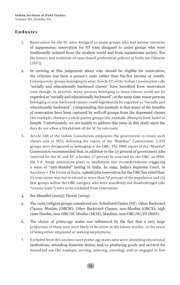
1. Reservation for the SC were designed to assist groups who had known centuries of suppression; reservation for ST were designed to assist groups who were traditionally isolated from the modern world and from mainstream society. For the history and evolution of caste-based preferential policies in India see Osborne (2001).

2. In arriving at this judgement about who should be eligible for reservation, the criterion has been a person’s caste rather than his/her income or wealth. Consequently, groups belonging to what Article 115 of the Indian Constitution calls “socially and educationally backward classes” have benefited from reservation even though, in practice, many persons belonging to these classes could not be regarded as “socially and educationally backward”; at the same time, many persons belonging to non-backward classes could legitimately be regarded as “socially and educationally backward”. Compounding this anomaly is that many of the benefits of reservation have been captured by well-off groups from the depressed classes (for example, chamars ) while poorer groups (for example, bhangis) have failed to benefit. Unfortunately, we are unable to address this issue in this study since the data do not allow a breakdown of the SC by sub-caste.

3. Article 340 of the Indian Constitution empowers the government to create such classes and in 1955, following the report of the “Kalelkar” Commission, 2,339 groups were designated as belonging to the OBC. The 1980 report of the “Mandal” Commission recommended that, in addition to the 23 percent of government jobs reserved for the SC and ST, a further 27 percent be reserved for the OBC. In 1990, the V.P. Singh announced plans to implement this recommendation triggering a wave of “anti-Mandal” rioting in India. In 1992, India’s Supreme Court, in Sawhney v The Union of India, upheld jobs reservation for the OBC but ruled that: (i) reservation was not to extend to more than 50 percent of the population and (ii) that groups within the OBC category who were manifestly not disadvantaged (the “creamy layer”) were to be excluded from reservation.

4. See Bhambri (2005); Thorat (2005).

5. The caste/religion groups considered are: Scheduled Castes (S)C; Other Backward Classes, Muslim (OBCM); Other Backward Classes, non-Muslim (OBCX); high caste Hindus, non-OBC/SC Hindus (HCH); Muslims, non-OBC/SC/ST (MSX).

6. The choice of prime-age males was influenced by the fact that a very large proportion of these men were likely to be active in the labour market, in the sense of being either employed or seeking employment.

7. Excluded from this analysis were prime-age males who were: attending educational institutions; attending domestic duties, and/or producing goods and services for household use (for example, serving, tailoring, weaving), and/or engaged in free

39


collection of goods - for example, vegetables, roots, firewood, cattle feed; rentiers, pensioners, and remittance recipients unable to work owing to a disability; beggars and prostitutes; and “others”.

8. However, there may be cases where self-employment is the preferred outcome over the available choices. We are unable to take account of such preferences because all we observe is the outcome and not the reasons for the outcome.

9. That is, Hindus who did not belong to the SC/ST or to the OBC.

10. With J mutually exclusive and collectively exhaustive outcomes, indexed 1…J, the multinomial logit model is defined by a pair of equations. The first, defines the log

odds ratio of a person i being in status j>1, relative to being in the ‘base’ status j=J,

as a linear function of { , 1... }ikX k K= =iX , the vector of values of K explanatory

variables ( 1 1iX = ) for the person: ( )( ) ∑

=

==

== K

kjijkjk

i

i XXJYJY

1PrPr

log ββ where:

Yi is an integer variable which takes the value j if, and only if, outcome j occurs

for person i, and jβ is the vector of coefficients associated with outcome j, 1jβbeing the coefficient associated with the intercept term. The second equation defines the probability of outcome j (j=1…J) occurring for individual i as:

( ) ( ) ( )ji

J

ririji XFZZjY β=

+== ∑

=1

1/expPr

11. However, the direction of change in the probability of an outcome, consequent

upon a unit change in ikX , cannot be inferred from the sign of jkβ . The reason is that, in a multinomial model, a change in the value of a variable for a person changes the probability of every outcome for him/her. Since these changes are constrained to sum to zero, whether the probability of a particular outcome goes up or down depends on what happens to the probabilities of the other outcomes.

12. By definition, an unemployed person did not work on any day of the week.

13. See Oaxaca (1973), Blinder (1973).

14. Other tables are not shown but available on request from the author.

40


References

Akerlof, G.A. and Kranton, R.E. (2010), Identity Economics: How Our Identities Shape Our Work, Wages, and Well-Being, Princeton, NJ: Princeton University Press.

Borooah, V.K., McKee, P.M., Heaton, N.E., and Collins, G. (1995), “Catholic Protestant Income Differences in Northern Ireland”, Review of Income and Wealth, 41, 1-16.Borooah, V.K. (2001), “How do Employees of Ethnic Origin Fare on Britain’s Occupational Ladder”, Scottish Journal of Political Economy, 48, 1-26.Borooah, V.K., Dubey, A., and Iyer, S. (2007), “The Effectiveness of Jobs Reservation: Caste, Religion, and Economic Status in India”, Development & Change, 38, 423-455.

Dhesi, A.S. and Singh, H. “Education, Labour Market Distortions and Relative Earnings of Different Religion-Caste Categories in India (A C ase S tudy of D elhi)”, Canadian Journal of Development Studies, 10: 75-89.

Esteve-Bolart, B (2004), Gender Discrimination and Growth: Theory and Evidence from India, Suntory and Toyota International Centres for Economics and Related Disciplines, London School of Economics and Political Science, London, UK.

Harkness, S. (1996), “The Gender Earnings Gap: Evidence from the UK”, Fiscal Studies, 17, 1-36.

Ito, T., (2009), “Caste discrimination and transaction costs in the labor market: Evidence from rural North India”, Journal of Development Economics, 88: 292–300.

Jeffery, R. and Jeffery, P. (1997), Population, Gender and Politics, Cambridge: Cambridge University Press.

Madeshwaran, S. and Attewell, P. (2007), “Caste Discrimination in the Indian Urban Market: Evidence from the National Sample Survey”, Economic and Political Weekly, 42: 4146-4153.

Nambissan, G.B. (2010), “Exclusion and Discrimination in Schools”, in S. Throat and K. S. Newman (edited), Blocked by Caste: Economic Discrimination in Modern India, New Delhi: Oxford University Press, pp. 253-286.

Neumark, D. (1988), “Employers’ Discriminatory behavior and the Estimation of Wage Discrimination”, Journal of Human Resources, 23, 279-295.

Nielsen, H.S. (1998), “Discrimination and Detailed Decomposition in a Logit Model”, Economics Letters, 61, 115-20.

Oaxaca, R. (1973), “Male-Female Wage Differentials in Urban Labor Markets”, International Economic Review, vol. 14, pp. 693-709.

Oaxaca, R. and Ransom, M.R. (1994), “On Discrimination and the Decomposition of Wage Differentials”, Journal of Econometrics, 61, 5-21.

Ramachandran, V. and Naorem, T. (2013), What it Means to be a Dalit or Tribal Child in our Schools, Economic and Political Weekly, vol XLVIII No. 44, November.

Reimers, C.W. (1983), “Labour Market Discrimination against Hispanic and Black Men”, Review of Economics and Statistics, 65, 570-579.

Schmidt, P. and Strauss, R.P. (1975), “The Prediction of Occupation Using Multiple Logit Models”, International Economic Review, 16, 570-579.

Thorat and Attewell, P. (2007) “A Legacy of Social Discrimination: A Correspondence Study of Job Discrimination in India”, Economic and Political Weekly, 42: 4141-4145.

The views expressed in this working paper are those of the author (s) andnot necessarily endorsed by or representative of Indian Institute of Dalit Studies or the co-sponsoring or supporting organizations

Copyright ©2013 Indian Institute of Dalit Studies. All rights reserved.

I N D I A N I N S T I T U T E O F D A L I T S T U D I E S

Devoted to Studies on Social Exclusion, Marginalised Groups and Inclusive Policies

IND IAN INST I TUTE OF DAL I T S TUD IESD-ll/l, Road No. 4, Andrews Ganj, New Delhi 110 049T: +91-11-26252082 [email protected]

WORKING PAPER SERIESVolume VII Number 04, 2013

Caste, Employment, and Wages in India: How do Employees from Different Social Groups Fare in India’s Labour Market?

VAN I K BOROOAH

N IDH I SADANA SABHARWAL

A J AYA KUMAR NA I K

INDIAN

INST

ITUTE OF DALIT

STU

DIES

INDIAN

INST

ITUTE OF DALIT

STU

DIES INDIAN

INST

ITUTE OF DALIT

STU

DIES

Caste, Employment, and Wages in India: How do …€¦ · · 2018-01-23A Model of Wage Rate...

Documents

Transcript of Caste, Employment, and Wages in India: How do …€¦ · · 2018-01-23A Model of Wage Rate...