Case Study: Generalized Lasso Problems

Ryan TibshiraniConvex Optimization 10-725/36-725

1

Last time: review of optimization toolbox

So far we’ve learned about:

• First-order methods

• Newton/quasi-Newton methods

• Interior point methods

These comprise a good part of the core tools in optimization, andare a big focus in this field

(Still, there’s a lot more out there. Before the course is over we’llcover dual methods and ADMM, coordinate descent, proximal andprojected Newton ...)

Given the number of available tools, it may seem overwhelming tochoose a method in practice. A fair question: how to know whatto use when?

2

It’s not possible to give a complete answer to this question. Butthe big algorithms table from last time gave guidelines. It covered:

• Assumptions on criterion function

• Assumptions on constraint functions/set

• Ease of implementation (how to choose parameters?)

• Cost of each iteration

• Number of iterations needed

Other important aspects, that it didn’t consider: parallelization,data storage issues, statistical interplay

Here, as any example, we walk through some of the high-levelreasoning for related but distinct generalized lasso problem cases

3

Generalized lasso problems

Consider the problem

minβ

f(β) + λ‖Dβ‖1

where f : Rn → R is a smooth, convex function and D ∈ Rm×n isa penalty matrix. This is called a generalized lasso problem

The usual lasso, D = I, encodes sparsity in solution β, while thegeneralized lasso encodes sparsity in

Dβ =

D1β...

Dmβ

where D1, . . . Dm are the rows of D. This can result in interestingstructure in β, depending on choice of D

4

Outline

Today:

• Notable examples

• Algorithmic considerations

• Back to examples

• Implementation tips

5

Fused lasso or total variation denoising, 1d

Special case: fused lasso or total variation denoising in 1d, where

D =

−1 1 0 . . . 0 00 −1 1 . . . 0 0...0 0 0 . . . −1 1

, so ‖Dβ‖1 =n−1∑i=1

|βi − βi+1|

Now we obtain sparsity in adjacent differences βi − βi+1, i.e., weobtain βi = βi+1 at many locations i

Hence, plotted in order of the locations i = 1, . . . n, the solution βappears piecewise constant

6

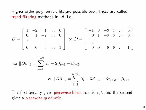
Examples:

Gaussian loss Logistic lossf(β) = 1

2

∑ni=1(yi − βi)2 f(β) =

∑ni=1(−yiβi + log(1 + eβi))

●

●

●

●

●●●

●

●

●

●

●

●

●●

●●●

●●

●

●

●

●●

●

●

●

●

●

●

●

●

●●

●

●

●

●●

●●

●●

●

●

●

●

●

●

●

●

●

●

●

●

●

●

●

●

●

●

●

●

●

●

●

●

●

●

●

●

●

●

●

●●

●●

●

●

●

●●

●

●

●●

●

●●

●

●

●

●

●

●

●●

●

0 20 40 60 80 100

−2

−1

01

2

●

●●●

●

●

●●

●●●●●●●●●●

●

●

●●●●●●●

●

●●●●●●●●●●●●●●●●●●●

●

●●●●●●

●●●●

●●

●●●●●●●●●●●●●●●●●●●●

●●●●●●●●●●●●

●

●●●●●●●

0 20 40 60 80 100

0.0

0.2

0.4

0.6

0.8

1.0

7

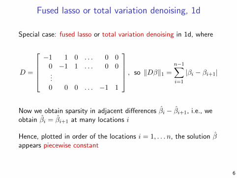
Higher order polynomials fits are possible too. These are calledtrend filtering methods in 1d, i.e.,

D =

1 −2 1 . . . 00 1 −2 . . . 0...0 0 0 . . . 1

or D =

−1 3 −3 1 . . . 00 1 −3 3 . . . 0...0 0 0 0 . . . 1

so ‖Dβ‖1 =n−2∑i=1

|βi − 2βi+1 + βi+2|

or ‖Dβ‖1 =n−3∑i=1

|βi − 3βi+1 + 3βi+2 − βi+3|

The first penalty gives piecewise linear solution β, and the secondgives a piecewise quadratic

8

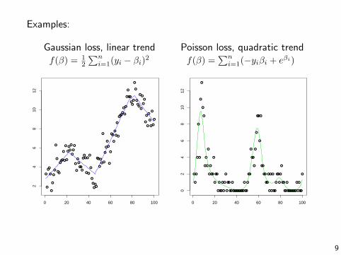
Examples:

Gaussian loss, linear trend Poisson loss, quadratic trendf(β) = 1

2

∑ni=1(yi − βi)2 f(β) =

∑ni=1(−yiβi + eβi)

●

●

●●

●

●

●

●

●

●

●

●●

●●●

●

●

●

●

●

●

●

●

●

●

●

●

●

●

●

●●

●

●●●

●

●

●

●

●

●

●

●

●●

●●

●

●

●

●

●

●

●

●

●

●

●

●●

●

●

●

●

●

●●●

●

●

●

●

●

●

●●

●●

●

●

●

●

●●

●

●

●

●

●

●

●

●

●

●

●

●

●

●

0 20 40 60 80 100

24

68

1012

●

●

●

●

●

●

●

●

●

●

●

●

●

●

●

●

●●

●

●

●●

●

●

●●

●

●

●

●

●

●●

●●

●

●●●●●●●●●●

●

●●

●

●●

●

●●

●

●

●

●●

●

●

●●

●●

●●

●

●

●

●

●

●●

●

●●

●

●

●

●●

●●

●

●●●●●●●●

●

●

●

●●

●

0 20 40 60 80 100

02

46

810

12

9

Fused lasso or total variation denoising, graphs

Special case: fused lasso or total variation denoising over a graph,G = ({1, . . . n}, E). Here D is |E| × n, and if e` = (i, j), then Dhas `th row

D` = (0, . . .−1↑i

, . . . 1↑j

, . . . 0)

so‖Dβ‖1 =

∑(i,j)∈E

|βi − βj |

Now at the solution, we get βi = βjacross many edges (i, j) ∈ E, so β ispiecewise constant over the graph G

10

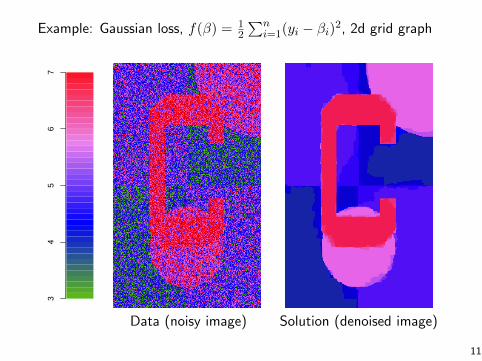
Example: Gaussian loss, f(β) = 12

∑ni=1(yi − βi)2, 2d grid graph

34

56

7

Data (noisy image) Solution (denoised image)

11

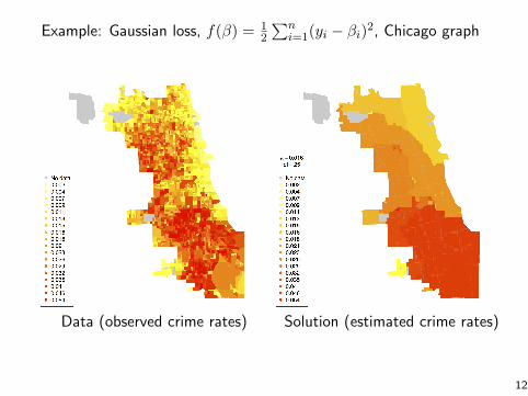
Example: Gaussian loss, f(β) = 12

∑ni=1(yi − βi)2, Chicago graph

Data (observed crime rates) Solution (estimated crime rates)

12

Problems with a big dense D

Special case: in some problems we encounter a big dense operatorD, whose structure might as well be considered arbitrary

E.g., we might have collected measurements that we know shouldlie mostly orthogonal to the desired estimate β, and we stack thesealong the rows of D, known as analyzing operator in this setup

E.g., equality-constrained lasso problems also fit into this case, as

minβ

f(β) + λ‖β‖1 subject to Aβ = 0

can be reparametrized by letting D ∈ Rn×r have columns to spannull(A). Then Aβ = 0 ⇐⇒ β = Dθ for some θ ∈ Rr, and theabove is equivalent to

minθ

f(Dθ) + λ‖Dθ‖1

13

Generalized lasso algorithms

Let’s go through our toolset, to figure out how to solve

minβ

f(β) + λ‖Dβ‖1

Subgradient method: subgradient of criterion is

g = ∇f(β) + λDTγ

where γ ∈ ∂‖x‖1 evaluated at x = Dβ, i.e.,

γi ∈

{{sign

((Dβ)i

)} if (Dβ)i 6= 0

[−1, 1] if (Dβ)i = 0, i = 1, . . .m

Downside (as usual) is that convergence is slow. Upside is that g iseasy to compute (provided ∇f is): if S = supp(Dβ), then we let

g = ∇f(β) + λ∑i∈S

sign((Dβ)i

)·Di

14

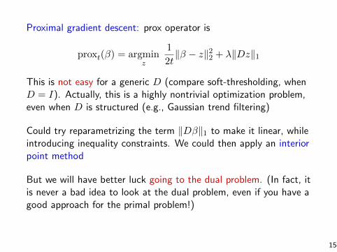
Proximal gradient descent: prox operator is

proxt(β) = argminz

1

2t‖β − z‖22 + λ‖Dz‖1

This is not easy for a generic D (compare soft-thresholding, whenD = I). Actually, this is a highly nontrivial optimization problem,even when D is structured (e.g., Gaussian trend filtering)

Could try reparametrizing the term ‖Dβ‖1 to make it linear, whileintroducing inequality constraints. We could then apply an interiorpoint method

But we will have better luck going to the dual problem. (In fact, itis never a bad idea to look at the dual problem, even if you have agood approach for the primal problem!)

15

Generalized lasso dualOur problems are

Primal : minβ

f(β) + λ‖Dβ‖1

Dual : minu

f∗(−DTu) subject to ‖u‖∞ ≤ λ

Here f∗ is the conjugate of f . Note that u ∈ Rm (where m is thenumber of rows of D) while β ∈ Rn

The primal and dual solutions β, u are linked by KKT conditions:

∇f(β) +DT u = 0, and

ui ∈

{λ} if (Dβ)i > 0

{−λ} if (Dβ)i < 0

[−λ, λ] if (Dβ)i = 0

, i = 1, . . .m

Second property implies that: ui ∈ (−λ, λ) =⇒ (Dβ)i = 0

16

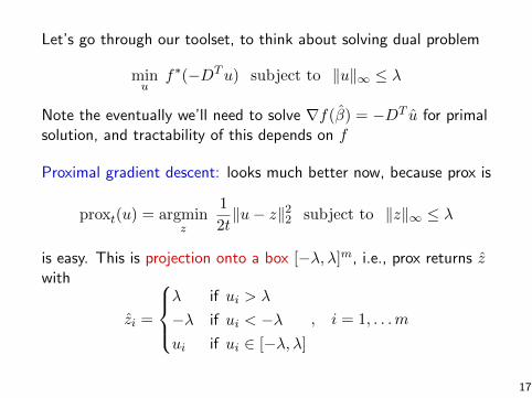
Let’s go through our toolset, to think about solving dual problem

minu

f∗(−DTu) subject to ‖u‖∞ ≤ λ

Note the eventually we’ll need to solve ∇f(β) = −DT u for primalsolution, and tractability of this depends on f

Proximal gradient descent: looks much better now, because prox is

proxt(u) = argminz

1

2t‖u− z‖22 subject to ‖z‖∞ ≤ λ

is easy. This is projection onto a box [−λ, λ]m, i.e., prox returns zwith

zi =

λ if ui > λ

−λ if ui < −λui if ui ∈ [−λ, λ]

, i = 1, . . .m

17

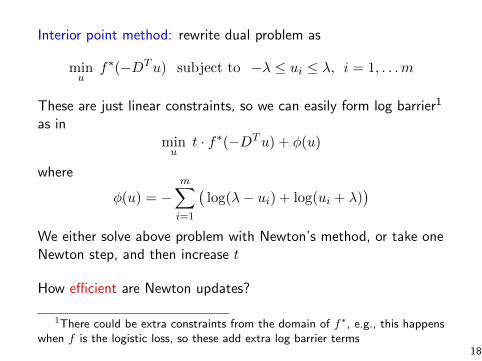
Interior point method: rewrite dual problem as

minu

f∗(−DTu) subject to −λ ≤ ui ≤ λ, i = 1, . . .m

These are just linear constraints, so we can easily form log barrier1

as inminu

t · f∗(−DTu) + φ(u)

where

φ(u) = −m∑i=1

(log(λ− ui) + log(ui + λ)

)We either solve above problem with Newton’s method, or take oneNewton step, and then increase t

How efficient are Newton updates?

1There could be extra constraints from the domain of f∗, e.g., this happenswhen f is the logistic loss, so these add extra log barrier terms

18

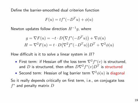
Define the barrier-smoothed dual criterion function

F (u) = tf∗(−DTu) + φ(u)

Newton updates follow direction H−1g, where

g = ∇F (u) = −t ·D(∇f∗(−DTu)

)+∇φ(u)

H = ∇2F (u) = t ·D(∇2f∗(−DTu)

)DT +∇2φ(u)

How difficult is it to solve a linear system in H?

• First term: if Hessian off the loss term ∇2f∗(v) is structured,and D is structured, then often D∇2f∗(v)DT is structured

• Second term: Hessian of log barrier term ∇2φ(u) is diagonal

So it really depends critically on first term, i.e., on conjugate lossf∗ and penalty matrix D

19

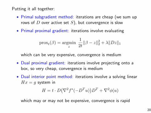
Putting it all together:

• Primal subgradient method: iterations are cheap (we sum uprows of D over active set S), but convergence is slow

• Primal proximal gradient: iterations involve evaluating

proxt(β) = argminz

1

2t‖β − z‖22 + λ‖Dz‖1

which can be very expensive, convergence is medium

• Dual proximal gradient: iterations involve projecting onto abox, so very cheap, convergence is medium

• Dual interior point method: iterations involve a solving linearHx = g system in

H = t ·D(∇2f∗(−DTu)

)DT +∇2φ(u)

which may or may not be expensive, convergence is rapid

20

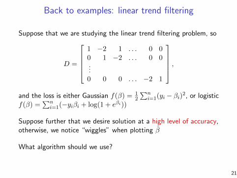
Back to examples: linear trend filtering

Suppose that we are studying the linear trend filtering problem, so

D =

1 −2 1 . . . 0 00 1 −2 . . . 0 0...0 0 0 . . . −2 1

,and the loss is either Gaussian f(β) = 1

2

∑ni=1(yi − βi)2, or logistic

f(β) =∑n

i=1(−yiβi + log(1 + eβi))

Suppose further that we desire solution at a high level of accuracy,otherwise, we notice “wiggles” when plotting β

What algorithm should we use?

21

Primal subgradient and primal proximal gradient are out (slow andintractable, respectively)

As for dual algorithms, one can check that the conjugate f∗ has aclosed-form for both the Gaussian and logistic cases:

f∗(v) =1

2

n∑i=1

y2i −1

2

n∑i=1

(yi + vi)2 and

f∗(v) =

n∑i=1

((vi + yi) log(vi + yi) + (1− vi − yi) log(1− vi − yi)

)respectively. We also the have expressions for primal solutions

β = y −DT u and

βi = −yi log(yi(D

T u)i)+ yi log

(1− yi(DT u)i

), i = 1, . . . n

respectively

22

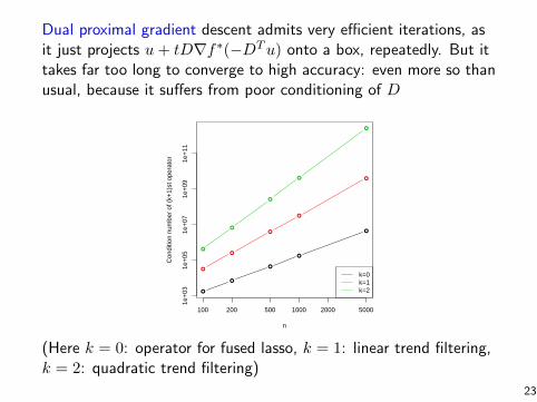
Dual proximal gradient descent admits very efficient iterations, asit just projects u+ tD∇f∗(−DTu) onto a box, repeatedly. But ittakes far too long to converge to high accuracy: even more so thanusual, because it suffers from poor conditioning of D

●

●

●

●

●

100 200 500 1000 2000 5000

1e+

031e

+05

1e+

071e

+09

1e+

11

n

Con

ditio

n nu

mbe

r of

(k+

1)st

ope

rato

r

●

●

●

●

●

●

●

●

●

●

k=0k=1k=2

(Here k = 0: operator for fused lasso, k = 1: linear trend filtering,k = 2: quadratic trend filtering)

23

Importantly, ∇2f∗(v) is a diagonal matrix in both the Gaussianand logistic cases:

∇2f∗(v) = I and

∇2f∗(v) = diag

(1

vi + yi+

1

1− vi − yi, i = 1, . . .m

)respectively. Therefore the Newton steps in a dual interior pointmethod involve solving a linear system Hx = g in

H = DA(u)DT +B(u)

where A(u), B(u) are both diagonal. This is a banded matrix, andso these systems can be solved very efficiently, in O(n) flops

Hence, an interior point method on the dual problem is the way togo: cheap iterations, and convergence to high accuracy is very fast

24

Recall example from our first lecture:

●

●

●●

●

●

●

●●

●

●

●●

●●●

●

●

●

●

●

●●

●

●

●

●

●

●

●●●●●

●

●●

●

●

●

●

●

●●●●

●

●●

●

●

●

●

●

●●●

●

●

●

●●

●

●

●

●

●

●●●●●

●

●

●

●

●●

●

●

●

●●

●●●

●

●

●

●

●

●

●

●

●●●

●

●

●●

●●

●

●

●

●

●

●

●

●

●

●●

●

●

●

●●●●●

●●●

●●

●

●

●

●

●

●

●

●

●●●●●

●

●●

●●●●

●

●

●

●

●

●

●

●

●

●

●

●●

●

●

●

●

●●

●

●

●

●

●

●

●●●

●

●

●●

●

●●●

●●

●●

●

●

●

●●

●

●

●

●

●

●●●

●●

●

●●

●

●

●

●

●

●

●

●

●

●●

●

●

●

●

●

●

●

●

●

●

●

●

●

●

●

●●

●

●

●

●

●

●

●

●

●

●

●

●

●

●

●

●●

●

●●

●

●

●●

●

●

●●●

●

●

●

●

●

●

●

●

●

●

●

●

●

●

●

●

●

●

●

●

●●●

●

●

●

●●

●

●

●

●●●

●

●●

●●

●

●

●

●

●

●

●●●

●

●●

●●

●

●

●

●

●

●

●●●

●●

●

●

●

●

●●

●●

●

●●●●

●

●

●

●●●

●

●●●

●

●

●

●

●

●●

●

●

●

●

●

●●

●

●

●

●

●

●

●

●

●

●●

●

●

●

●●●

●

●●●

●●●

●

●

●

●

●

●

●●

●●

●

●●●

●

●●

●

●

●

●

●

●

●●

●

●

●

●

●

●

●

●

●

●

●●

●

●

●

●

●

●

●●

●

●

●

●

●

●

●

●

●

●●●●

●

●

●

●

●

●

●

●

●

●

●

●

●

●

●

●

●

●

●

●●

●

●

●

●●

●

●●

●●

●

●

●●

●

●

●

●

●

●

●

●

●

●

●

●

●●●

●●

●

●

●●

●

●

●

●●●

●

●

●●

●●●

●

●

●

●

●

●

●●

●●●

●

●

●

●

●

●

●

●

●

●

●

●

●●

●

●●

●

●

●

●

●

●

●

●

●

●

●

●

●●

●●●

●●●●●

●●

●

●

●

●

●●●

●

●

●●

●

●●

●●●●●

●

●

●

●

●

●

●●

●

●

●

●

●

●

●

●

●●

●●

●●

●

●

●●

●

●

●

●

●

●

●

●

●

●

●

●

●

●

●●

●

●

●

●

●●

●

●

●●

●

●●

●

●●

●

●

●

●

●●●

●

●

●

●

●●●

●●

●

●

●

●

●

●

●●

●●

●

●●●●●

●

●

●●

●

●●

●

●●

●

●

●

●●

●●

●●

●

●

●

●

●

●

●●

●

●

●

●

●●●●●

●

●

●

●

●●

●●

●

●

●

●

●●

●

●

●

●

●

●

●●●

●

●

●

●

●●

●

●

●●

●

●

●

●●

●

●

●

●●

●●●

●

●●●

●

●

●●

●

●

●●

●●

●

●

●●

●

●

●

●

●

●●

●

●●

●

●

●

●

●

●●

●

●

●●

●

●●

●

●●

●

●●

●

●●

●

●

●

●

●

●●

●

●

●

●

●

●

●

●●●

●

●

●

●●

●

●●

●

●

●

●

●

●

●

●

●

●●●●

●

●●

●

●

●

●●

●

●●●

●

●

●

●

●

●

●

●

●

●●

●

●

●

●

●

●

●

●

●

●

●

●

●●●●

●●●

●●

●●●

●●

●

●●●

●●●

●●

●

●●

●

●

●

●

●

●●●

●

●

●

●●

●

●

●

●

●

●●

●●

●

●

●

●

●

●

●●

●

●●

●

●

●●●●

●

●

●

●

●

●

●

●

●

●●

●

●

●

●

●

●

●

●●

●●

●

●

●

●

●●

●

●●

●

●●

●

●

●●

●

●

●

●

●

●

●●

●●●

●

●

●●

●

0 200 400 600 800 1000

05

10

Timepoint

Act

ivat

ion

leve

l

●

●

●●

●

●

●

●●

●

●

●●

●●●

●

●

●

●

●

●●

●

●

●

●

●

●

●●●●●

●

●●

●

●

●

●

●

●●●●

●

●●

●

●

●

●

●

●●●

●

●

●

●●

●

●

●

●

●

●●●●●

●

●

●

●

●●

●

●

●

●●

●●●

●

●

●

●

●

●

●

●

●●●

●

●

●●

●●

●

●

●

●

●

●

●

●

●

●●

●

●

●

●●●●●

●●●

●●

●

●

●

●

●

●

●

●

●●●●●

●

●●

●●●●

●

●

●

●

●

●

●

●

●

●

●

●●

●

●

●

●

●●

●

●

●

●

●

●

●●●

●

●

●●

●

●●●

●●

●●

●

●

●

●●

●

●

●

●

●

●●●

●●

●

●●

●

●

●

●

●

●

●

●

●

●●

●

●

●

●

●

●

●

●

●

●

●

●

●

●

●

●●

●

●

●

●

●

●

●

●

●

●

●

●

●

●

●

●●

●

●●

●

●

●●

●

●

●●●

●

●

●

●

●

●

●

●

●

●

●

●

●

●

●

●

●

●

●

●

●●●

●

●

●

●●

●

●

●

●●●

●

●●

●●

●

●

●

●

●

●

●●●

●

●●

●●

●

●

●

●

●

●

●●●

●●

●

●

●

●

●●

●●

●

●●●●

●

●

●

●●●

●

●●●

●

●

●

●

●

●●

●

●

●

●

●

●●

●

●

●

●

●

●

●

●

●

●●

●

●

●

●●●

●

●●●

●●●

●

●

●

●

●

●

●●

●●

●

●●●

●

●●

●

●

●

●

●

●

●●

●

●

●

●

●

●

●

●

●

●

●●

●

●

●

●

●

●

●●

●

●

●

●

●

●

●

●

●

●●●●

●

●

●

●

●

●

●

●

●

●

●

●

●

●

●

●

●

●

●

●●

●

●

●

●●

●

●●

●●

●

●

●●

●

●

●

●

●

●

●

●

●

●

●

●

●●●

●●

●

●

●●

●

●

●

●●●

●

●

●●

●●●

●

●

●

●

●

●

●●

●●●

●

●

●

●

●

●

●

●

●

●

●

●

●●

●

●●

●

●

●

●

●

●

●

●

●

●

●

●

●●

●●●

●●●●●

●●

●

●

●

●

●●●

●

●

●●

●

●●

●●●●●

●

●

●

●

●

●

●●

●

●

●

●

●

●

●

●

●●

●●

●●

●

●

●●

●

●

●

●

●

●

●

●

●

●

●

●

●

●

●●

●

●

●

●

●●

●

●

●●

●

●●

●

●●

●

●

●

●

●●●

●

●

●

●

●●●

●●

●

●

●

●

●

●

●●

●●

●

●●●●●

●

●

●●

●

●●

●

●●

●

●

●

●●

●●

●●

●

●

●

●

●

●

●●

●

●

●

●

●●●●●

●

●

●

●

●●

●●

●

●

●

●

●●

●

●

●

●

●

●

●●●

●

●

●

●

●●

●

●

●●

●

●

●

●●

●

●

●

●●

●●●

●

●●●

●

●

●●

●

●

●●

●●

●

●

●●

●

●

●

●

●

●●

●

●●

●

●

●

●

●

●●

●

●

●●

●

●●

●

●●

●

●●

●

●●

●

●

●

●

●

●●

●

●

●

●

●

●

●

●●●

●

●

●

●●

●

●●

●

●

●

●

●

●

●

●

●

●●●●

●

●●

●

●

●

●●

●

●●●

●

●

●

●

●

●

●

●

●

●●

●

●

●

●

●

●

●

●

●

●

●

●

●●●●

●●●

●●

●●●

●●

●

●●●

●●●

●●

●

●●

●

●

●

●

●

●●●

●

●

●

●●

●

●

●

●

●

●●

●●

●

●

●

●

●

●

●●

●

●●

●

●

●●●●

●

●

●

●

●

●

●

●

●

●●

●

●

●

●

●

●

●

●●

●●

●

●

●

●

●●

●

●●

●

●●

●

●

●●

●

●

●

●

●

●

●●

●●●

●

●

●●

●

0 200 400 600 800 1000

05

10Timepoint

Act

ivat

ion

leve

l

Dual interior point method20 iterations

Dual proximal gradient10,000 iterations

25

Back to examples: graph fused lasso

Essentially the same story holds when D is the fused lasso operatoron an arbitrary graph:

• Primal subgradient is slow, primal prox is intractable

• Dual prox is cheap to iterate, but slow to converge

• Dual interior point method solves structured linear systems, soits iterations are efficient, and is preferred

Dual interior point method repeatedly solves Hx = g, where

H = DA(u)DT +B(u)

and A(u), B(u) are both diagonal. This no longer banded, but it ishighly structured: D is the edge incidence matrix of the graph, andL = DTD the graph Laplacian

But the story can suddenly change, with a tweak to the problem!

26

Back to examples: regression problems

Consider the same D, and the same Gaussian and logistic losses,but with regressors or predictors xi ∈ Rp, i = 1, . . . n,

f(β) =1

2

n∑i=1

(yi − xTi β)2 and

f(β) =

n∑i=1

(− yixTi β + log(1 + exp(xTi β)

)respectively. E.g., if the predictors are connected over a graph, andD is the graph fused lasso matrix, then the estimated coefficientswill be constant over regions of the graph

Assume that the predictors values are arbitrary. Everything in thedual is more complicated now

27

Denote X ∈ Rn×p as the predictor matrix (rows xi, i = 1, . . . n),and f(β) = h(Xβ) as the loss. Our problems are

Primal : minβ

h(Xβ) + λ‖Dβ‖1

Dual : minu,v

h∗(v)

subject to XT v +DTu = 0, ‖u‖∞ ≤ λ

Here h∗ is the conjugate of h. Note that we have u ∈ Rm, v ∈ Rp.Furthermore, the primal and dual solutions β and u, v satisfy

∇h(Xβ)− v = 0 or equivalently

XT∇h(Xβ) +DT u = 0

Computing β from the dual requires solving a linear system in X,very expensive for generic X

28

Dual proximal gradient descent has become intractable, becausethe prox operator is

proxt(u, v) = argminXTw+DT z=0

1

2t‖u− z‖22 +

1

2t‖v − w‖22 + ‖u‖∞

This is finding the projection of (u, v) onto the intersection of aplane and a (lower-dimensional) box

Dual interior point methods also don’t look nearly as favorable asbefore, because the equality constraint

XT v +DTu = 0

must be maintained, so we augment the inner linear systems, andthis ruins their structure, since X is assumed to be dense

Primal subgradient method is still very slow. Must we use it?

29

In fact, for large and dense X, our best option is probably to useprimal proximal gradient descent. The gradient

∇f(β) = XT∇h(Xβ)

is easily computed via the chain rule, and the prox operator

proxt(β) = argminz

1

2t‖β − z‖22 + λ‖Dz‖1

is not evaluable in closed-form, but it is precisely the same problemwe considered solving before: graph fused lasso with Gaussian loss,and without regressors

Hence to (approximately) evaluate the prox, we run a dual interiorpoint method until convergence. We have freed ourselves entirelyfrom solving linear systems in X

30

(a) fold 1 (b) fold 3 (c) fold 5 (d) fold 7 (e) fold 9 (f) overlap

Figure 4: Consistency of selected voxels in different trials of cross-validations. The results of 5 different folds of cross-validations are shownin (a)-(e) and the overlapping voxels in all 10 folds are shown in (f). The top row shows the results for GFL and the bottom row shows theresults for L1. The percentages of the overlapping voxels were: GFL(66%) vs. L1(22%).

Table 1: Comparison of the accuracy of AD classification.

Task LR SVM LR+L1 LR+GFLAD/NC 80.45% 82.71% 81.20% 84.21%

MCI 63.83% 67.38% 68.79% 70.92%

We compared GFL to logistic regression (LR), supportvector machine (SVM), and logistic regression with anL1 regularizer. The classification accuracies obtained basedon a 10-fold cross validation (CV) are shown in Table 1,which shows that GFL yields the highest accuracy in bothtasks. Furthermore, compared with other reported results,our performance are comparable with the state-of-the-art.In (Cheng, Zhang, and Shen 2012), the best performancewith MCI tasks is 69.4% but our method reached 70.92%.In (Chu et al. 2012), a similar sample size is used as in ourexperiments, the performance of our method with ADNCtasks is comparable to or better than their reported results(84.21% vs. 81-84%) whereas our performance with MCItasks is much better (70.92% vs. 65%).

We applied GFL to all the samples where the optimal pa-rameter settings were determined by cross-validation. Figure5 compares the selected voxels with non-structured sparsity(i.e. L1), which shows that the voxels selected by GFL clus-tered into several spatially connected regions, whereas thevoxels selected by L1 were more scattered. We consideredthe voxels that corresponded to the top 50 negative �i’s asthe most atrophied voxels and projected them onto a slice.The results show that the voxels selected by GFL were con-centrated in hippocampus, parahippocampal gyrus, whichare believed to be the regions with early damage that areassociated with AD. By contrast, L1 selected either less crit-ical voxels or noisy voxels, which were not in the regionswith early damage (see Figure 5(b) and 5(c) for details).The voxels selected by GFL were also much more consistentthan those selected by L1, where the percentages of overlap-ping voxels according to the 10-fold cross-validation were:

(a) (b) (c)

Figure 5: Comparison of GFL and L1. The top row shows theselected voxels in a 3D brain model, the middle row shows thetop 50 atrophied voxels, and the bottom row shows the projec-tion onto a brain slice. (a) GFL (accuracy=84.21%); (b) L1 (ac-curacy=81.20%); (c) L1 (similar number of voxels as in GFL).

GFL=66% vs. L1=22%, as shown in Figure 4.

ConclusionsIn this study, we proposed an efficient and scalable algo-rithm for GFL. We demonstrated that the proposed algo-rithm performs significantly better than existing algorithms.By exploiting the efficiency and scalability of the proposedalgorithm, we formulated the diagnosis of AD as GFL. Ourevaluations showed that GFL delivered state-of-the-art clas-sification accuracy and the selected critical voxels were wellstructured.

2168

(From Xin et al. (2014), “Efficient generalized fused lasso and itsapplication to the diagnosis of Alzheimer’s disease”)

31

Relative importance: dementia vs normal

0 20 40 60 80 100

trust03.3

digcor

sick03.2

grpsym09.1

pulse21

orthos27

race01.1

hctz06

gend01

early39

fear05.1

estrop39

newthg68.1

cdays59

race01.2

β..1: dementia vs normal

65 70 75 80 85 90 95 100

−0.

2−

0.1

0.0

0.1

0.2

fear05.1sick03.2newthg68.1early39hctz06grpsym09.1orthos27race01.1gend01trust03.3pulse21digcorcdays59estrop39race01.2

Coe

ffici

ents

Age

Relative importance: death vs normal

0 20 40 60 80 100

whmile09.2

ltaai

anyone

diabada.3

nomeds06

exer59

hlth159.1

smoke.3

dig06

numcig59

hurry59.2

cis42

gend01

ctime27

digcor

β..2: death vs normal

65 70 75 80 85 90 95 100

−0.

2−

0.1

0.0

0.1

0.2

ctime27numcig59cis42diabada.3hlth159.1dig06whmile09.2nomeds06anyoneexer59ltaaihurry59.2smoke.3gend01digcor

Coe

ffici

ents

Age

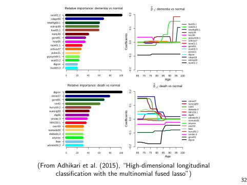
(From Adhikari et al. (2015), “High-dimensional longitudinalclassification with the multinomial fused lasso”)

32

Back to examples: 1d fused lasso

Let’s turn to the special case of the fused lasso in 1d, recall

D =

−1 1 0 . . . 0 00 −1 1 . . . 0 0...0 0 0 . . . −1 1

The prox function in the primal is

proxt(β) = argminz

1

2t‖β − z‖22 + λ

n∑i=1

|zi − zi+1|

This can be directly computed using specialized approaches such asdynamic programming2 or taut-string methods3 in O(n) operations

2Johnson (2013), “A dynamic programming algorithm for the fused lassoand L0-segmentation”

3Davies and Kovac (2001), “Local extremes, runs, strings, multiresolution”33

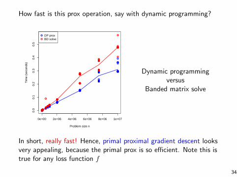
How fast is this prox operation, say with dynamic programming?

●●●●●●●●●●●●●●●●●●●●●●●●●●●●●●●●●●●●●●●●●●●●●●●●●●●●●●●●●●●●●●●●●●●●●●●●●●●●●●●●●●●●●●●●●●●●●●●●●●●●

●●●●●●●●●●●●●●●●●●●●●●●●●●●●●●●●●●●●●●●●●●●●●●●●●●

●●●●●●●●●●●●●●●●●●●●●●●●●

●●●●●●●●●●●●●●●●●●●●●●●●●

●●●●●●●●●●●●●●●●●●●●●●●●●

●●●

●

●

●

●

●

●

●

●

●

●

●

●

●

●

●

●

●

●

●

●

●

●

●

●

●●●

●

●

●●●●●●●●●●●●●●●●●●

0e+00 2e+06 4e+06 6e+06 8e+06 1e+07

0.0

0.1

0.2

0.3

0.4

0.5

Problem size n

Tim

e (s

econ

ds)

●●●●●●●●●●●●●●●●●●●●●●●●●●●●●●●●●●●●●●●●●●●●●●●●●●●●●●●●●●●●●●●●●●●●●●●●●●●●●●●●●●●●●●●●●●●●●●●●●●●●

●●●●●●●●●

●

●●●●●●●●●●●●●●●●●●●●●●●●●●●●●●●●●●●●●●●●

●●●●●●●●●●●●●●●●●●●●●●●●●

●●●●●●●●●●●●●●●●●●●●●●●●●

●●●●●

●●●●●●●●●●●●●●●●●●●●

●●

●

●

●

●

●

●

●

●

●

●

●

●

●

●

●

●

●

●

●

●

●

●

●

●

●●●

●

●●●●●●●●●●●●●●●●●●●●

●

●

DP proxBD solve

Dynamic programmingversus

Banded matrix solve

In short, really fast! Hence, primal proximal gradient descent looksvery appealing, because the primal prox is so efficient. Note this istrue for any loss function f

34

When f is the Gaussian or logistic losses, without predictors, bothprimal proximal gradient and dual interior point method are strongchoices. How do they compare? Logistic loss example, n = 2000:

●●●●●●●●●●●●●●●●●

●

●

●

●

●

●

●

●

●

●

●

●●●●●●●●●●●●●●●●●●●●●●●●●●●●●●●●●●●●●●●●●●●●●●●●●●●●

1e−03 1e−01 1e+01

020

040

060

080

010

00

lambda

prox

cou

nt

●●●●

●

●

●

●

●

●

●

●

●

●

●

●●●●●●●●●●●●●●●●●●●●●●●●●●●●●●●●●●●●●●●●●●●●●●●●●●●●●●●●●●●●●●●●●

●

●

coldwarm

●●●

●●

●

●

●

●

●●

●

●●●

●●

●

●●●●●

●

●●●●

●

●

●●

●●

●

●●

●●●

●

●●

●

●

●●

●

●

●

●●

●●

●

●

●

●

●

●

●●●

●●

●

●

●●

●●●

●●

●

●

●●

●●

1e−03 1e−01 1e+0140

6080

100

lambda

New

ton

coun

t

●

●●

●●●●

●

●

●●

●

●●●

●●

●

●●●●●

●

●●●●

●

●●

●●●

●

●●

●

●●

●

●

●

●

●

●●

●

●

●●●

●●

●

●

●

●

●

●

●●●

●●

●

●

●

●

●●●

●●

●●

●●

●●

●

●

coldwarm

Primal prox gradient is better for large λ, dual interior point betterfor small λ. Why this direction?

35

Primal : minβ

f(β) + λ‖Dβ‖1

Dual : minu

f∗(−DTu) subject to ‖u‖∞ ≤ λ

Observe:

• Large λ: many components (Dβ)i = 0 in primal, and manycomponents ui ∈ (−λ, λ) in dual

• Small λ: many components (Dβ)i 6= 0 in primal, and manycomponents |ui| = λ in dual

When many (Dβ)i = 0, there are fewer “effective parameters” inthe primal optimization; when many |ui| = λ, the same is true inthe dual

Hence, generally:

• Large λ: easier for primal algorithms

• Small λ: easier for dual algorithms

36

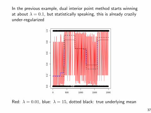
In the previous example, dual interior point method starts winningat about λ = 0.1, but statistically speaking, this is already crazilyunder-regularized

●●●●●●●●●●

●

●

●

●●●●●●●●●●●

●

●●

●

●●●●●●●●●●

●

●●●●●●●●

●

●●●●●●●

●●

●●●●●●●●●●●●

●

●●●●●●●●●●●●●●●●●●

●

●

●

●

●

●●●●●●●●●●●●●●

●

●●●●●●●

●●

●

●

●●●●●

●

●●●●●●●

●●

●●●●●●●●●●●●●

●

●

●

●●●●●●

●

●

●

●●●●●●●●

●

●●●●●●●●●●●●●●●●●●●●●●●●●

●

●●●

●

●●●●●●●

●

●●

●

●●●

●

●●●●●●●●●

●

●●●●●

●

●●●

●

●●●●●●●●●●●

●

●●●

●

●●●●●●●

●

●●●●●●●●●

●●

●●

●●●

●

●

●●●

●

●●

●

●●●

●●

●

●●

●●

●

●●●●

●●●

●●

●

●●●●

●

●

●

●

●

●●●●●

●

●●●●●●●●●●●●●●●●●

●

●●

●

●●●

●

●●●●●

●

●●●

●

●●●●●

●

●●

●

●●●●●

●

●●●●●●●●●●●

●

●●●●●●●●●

●

●

●●

●●

●

●●●●

●●●

●

●

●

●●●●

●●

●●●●●●●●●●●●●●●●

●

●●

●

●●●●●●●●●●●●●●●●

●

●●

●

●●●●●●

●

●●●●●●●

●

●●●●●

●

●●●●●●●●●●●

●

●●●●●●●

●

●●●●●●●●●●●●●

●

●●●●●●●●●●●●●●●●●●●

●

●●

●●

●●●●●●●●●●●

●

●●●●

●

●●●●●●●●●●●●●●●●●●●●●●

●

●●●●●●●●●●●

●

●●●●●●

●

●●●●●●●●●●●●

●

●●

●●

●●

●

●

●

●●●●●●●●●●●●●●●●●●

●

●●●●●●●●●●●●

●

●●●●●●

●

●●●●●●●●●●●●●●●●●●●●●●●●●●●●●●●●●●●●●●●●●●●●●●●●

●

●

●

●●●●●●●

●

●●●●●●●●●●●●●●●●●●●●●●●●●●●●●●●●●●●●●●●●●●●●●●●●●

●

●●●●●●●●●●●●●●

●

●●●●●

●

●●●●●●●●●●●●

●

●●●●●●●

●

●

●●

●●●

●

●●●●●

●

●●

●●

●

●

●●

●●●

●●●●

●●●●●

●●●

●●

●

●

●●●●●●●

●

●

●●

●

●

●●●

●

●●●●

●

●●●●●

●

●●

●●

●●●●●

●●

●

●●●

●

●●

●●●●●●●●●●●●●

●●

●●●●●●●●●

●●

●●●●

●●●

●

●●

●

●●●

●●●●

●

●●

●●●

●

●

●●

●

●●●●●

●●●

●●●

●

●●

●

●●●●●●●●●●

●●●●

●●

●

●●●●

●●

●●

●

●●●●●

●

●●●●●●

●

●●●●●

●

●

●

●●●●

●

●

●

●●

●

●

●●

●●●●

●

●

●

●

●

●●●

●

●●●

●

●●●●

●

●●●●●●●●●●

●

●●●

●●

●

●

●●●●

●●

●●

●

●●

●

●●●●●

●

●

●

●●●●●●●

●●

●●

●

●●

●

●●

●●

●●●

●●

●●●●●●●

●

●●

●

●

●●

●●

●

●

●

●

●

●

●●●

●●●●

●

●●●●●●●

●

●●●

●

●

●

●●●

●

●

●

●

●●●

●●●●●●●●●

●

●

●

●

●

●

●●

●●

●

●●

●

●●●●●●

●

●●●●●

●●

●●●

●●●

●●

●●●●●●●●●●

●

●

●●

●●●

●

●

●

●

●

●●●

●●

●●●●●●

●●

●●●●●●●

●●

●●●●●

●●●

●●●

●

●●●

●●

●

●

●

●

●●●

●●●

●●●●●

●

●●●

●

●●●●

●●

●●●

●

●●●

●

●●●●

●

●

●●

●●●

●

●●●

●

●●●●●

●●

●●●

●

●●

●

●

●●●

●●●

●

●●●●●●

●●●

●

●●●●●

●●

●●●

●

●

●●

●●

●●●

●●

●●●●

●

●●

●●

●●●●●

●

●●●●

●●

●

●

●●●●

●●

●●

●

●●●●

●

●●●●●●

●●●●

●

●

●●●●●●●●●●

●

●

●●

●●●

●

●●●●●●●●

●

●●

●

●●

●

●●

●

●●

●●

●●

●

●

●

●●●●●●

●●●

●●

●

●●●

●

●●●●●●

●●●

●●●●●

●

●

●●

●●

●

●●●●●

●

●

●

●

●

●●●

●

●

●

●●●●●●●

●

●●●●●

●

●●●●●●

●

●

●

●

●

●●

●

●●

●●

●●●●●●●

●●

●

●

●●●●●●

●

●●

●●

●●●●●

●

●●●●●●

●●

●●●●●●●●●●●

●

●●

●●●●●

●

●●●●

●

●●●●●●●●●●●

●

●●●

●

●●●●●●●

●

●●

●

●●●●●●●●●●●●●●●●●●

●

●●●●

●

●●●●●●●

●

●●

●

●●●●●

●●

●●●●

●

●●

●

●●●

●

●●

●

●

●

●●●●●●●●●●●●●●●●●●●●●●●●●

●

●●●●●●●

●

●●●

●

●●

●

●●●●●●●●●

●●

●●●●●

●

●●●●●●●●●●●●●●●●●●●●●●

●

●●●

●

●●●●●●●●●

●

●●●●

●

●●●●

●

●●●●●●●●●●●●

●

●●●●●●●●●

●

●●●●●●●●●●

●

●●

●

●●●●●●

●

●●●

●●

●●●●●●●●●●●●●

●

●●●●●●●●●●●●

●

●●●●●●●●●●●●●●●●●●●●●

●

●

●

●●●●●

●

●●

●

●●●●●●●●●●●●●

●

●●●

●

●●●●

●

●●●●●

●

●●

●

●●●●●●●●●●●

●

●●●●●●●●

●

●●●●●●●●●●●●

●

●

●

●●●●●●●●●●●●

●

●●●●●●●●●●●●●●

0 500 1000 1500 2000

0.0

0.2

0.4

0.6

0.8

1.0

Red: λ = 0.01, blue: λ = 15, dotted black: true underlying mean

37

Back to examples: big dense D

Consider a problem with a dense, generic D, e.g., as an observedanalyzing operator, or stemming from an equality-constrained lassoproblem

Primal prox is intractable, and a dual interior point method hasextremely costly Newton steps

But, provided that we can form f∗ (and relate the primal and dualsolutions), dual proximal gradient still features efficient iterations:the gradient computation D∇f∗(−DTu) is more expensive than itwould be if D were sparse and structured, but still not anywhere asexpensive as solving a linear system in D

Its iterations simply repeat projecting u+ tD∇f∗(−DTu) onto thebox [−λ, λ]m, hence, especially if we do not need a highly accuratesolution, dual proximal gradient is the best method

38

Finally, consider a twist on this problem in which D is dense andso massive that even fitting it in memory is a burden

Depending on f and its gradient, primal subgradient method mightbe the only feasible algorithm; recall the subgradient calculation

g = ∇f(β) + λ∑i∈S

sign((Dβ)i

)·Di

where S is the set of all i such that (Dβ)i 6= 0

If λ is large enough so that many (Dβ)i = 0, then we only need tofit a small part of D in memory (or, read a small part of D from afile) to perform subgradient updates

Combined with perhaps a stochastic trick in evaluating either partof g above, this could be effective at large scale

39

What did we learn from this?

From generalized lasso study (really, these are general principles):

• There is no single best method: performance depends greatlystructure of penalty, conjugate of loss, desired accuracy level,sought regularization level

• Duality is your friend: dual approaches offer complementarystrengths, move linear transformation from nonsmooth penaltyinto smooth loss, and strive in different regularization regime

• Regressors complicate duality: presence of predictor variablesin the loss complicate dual relationship, but proximal gradientwill reduce this to a problem without predictors

• Recognizing easy subproblems: if there is a subproblem that isspecialized and efficiently solvable, then work around it

• Limited memory at scale: for large problems, active set and/orstochastic methods may be only option

40

Your toolbox will only get bigger

There are still many algorithms to be learned. E.g., for generalizedlasso problems, depending on the setting, we may instead use:

• Alternating direction method of multipliers

• Proximal Newton’s method

• Projected Newton’s method

• Exact path-following methods

Remember, you don’t have to find/design the perfect optimizationalgorithm, just one that will work well for your problem!

For completeness, recall tools like cvx4 and tfocs5, if performanceis not a concern, or you don’t want to expend programming effort

4Grant and Boyd (2008), “Graph implementations for nonsmooth convexproblems”, http://cvxr.com/cvx/

5Beckter et al. (2011), “Templates for convex cone problems withapplications to sparse signal recovery”, http://cvxr.com/tfocs/

41

Implementation tips

Implementation details are not typically the focus of optimizationcourses, because in a sense, implementation skills are under-valued

Still an extremely important part of optimization. Considerations:

• Speed

• Robustness

• Simplicity

• Portability

First point doesn’t need to be explained. Robustness refers to thestability of implementation across various use cases. E.g., supposeour graph fused lasso solver supported edge weights. It performswell when weights are all close to uniform, but what happens underhighly nonuniform weights? Huge and small weights, mixed?

42

Simplicity and portability are often ignored. An implementationwith 20K lines of code may run fast, but what happens when a bugpops up? What happens when you pass it on to a friend? Tips:

• A constant-factor speedup is probably not worth a much morecomplicated implementation, especially if the latter is hard tomaintain, hard to extend

• Speed of convergence to higher accuracy may be worth a lossof simplicity

• Write the code bulk in a low-level language (like C or C++),so that it can port to R, Matlab, Python, Julia, etc.

• Don’t re-implement standard routines, this is often not worthyour time, and prone to bugs. Especially true for numericallinear algebra routines!

43

References

Some algorithms for generalized lasso problems:

• T. Arnold and R. Tibshirani (2014), “Efficientimplementations of the generalized lasso dual path algorithm”

• A. Barbero and S. Sra (2014), “Modular proximal optimizationfor multidimensional total-variation regularization”

• S.-J. Kim, K. Koh, S. Boyd, and D. Gorinevsky (2009), “`1trend filtering”

• A. Ramdas and R. Tibshirani (2014), “Fast and flexiblealgorithms for trend filtering”

• Y.-X. Wang, J. Sharpnack, A. Smola, and R. Tibshirani(2014), “Trend filtering on graphs”

44

Some implementations of generalized lasso algorithms:

• T. Arnold, V. Sadhanala, and R. Tibshirani (2015), glmgen,https://github.com/statsmaths/glmgen

• T. Arnold and Ryan Tibshirani, genlasso,http://cran.r-project.org/package=genlasso

• A. Barbero and S. Sra (2015), proxTV,https://github.com/albarji/proxTV

• J. Friedman, T. Hastie, and R. Tibshirani (2008), glmnet,http://cran.r-project.org/web/packages/glmnet

45