CAS Exam 5 Seminar Style Slides 2019...
131
CAS Exam 5 Seminar Style Slides 2019 Edition prepared by Howard C. Mahler, FCAS Copyright 2019 by Howard C. Mahler. Howard Mahler [email protected] www.howardmahler.com/Teaching
Transcript of CAS Exam 5 Seminar Style Slides 2019...

CAS Exam 5
Seminar Style Slides2019 Edition
prepared byHoward C. Mahler, FCAS
Copyright 2019 by Howard C. Mahler.
Howard [email protected]/Teaching

These are slides that I have presented at a seminar.
Covered is the ratemaking portion of CAS Exam 5.Not covered are the reserving topics on CAS Exam 5 which are covered in:“Estimating Unpaid Claims Using Basic Techniques,” by Jacqueline F. Friedland,Statement of Principles Regarding Property and Casualty Unpaid Claim Estimates, Casualty Actuarial Society, November 2014,and Actuarial Standard of Practice No. 43: Property/Casualty Unpaid Claim Estimates, American Academy of Actuaries, 2007 and Updated for Deviation Effective May 2011.
Use the bookmarks in the Navigation Panel in order to help you find what you want.
This provides another way to study the material. Some of you will find it helpful to go through a few sections at a time, either alone or with a someone else, pausing to do each of the problems included.Estimated time to go through all of the slides is about 35 hours.
Some of the problems were written by me and some are past exam questions so labeled.
All the material, problems, and solutions are in my study guide, sold separately. These slides are a useful supplement to my study guide, but are self-contained.There are references to page and problem numbers in the latest edition of my study guide, which you can ignore if you do not have my study guide.
The slides are in the same order as the sections of my study guide.At the end, there are some additional questions for study.
Section # Section NameA 1 Introduction
2 Rating Manuals3 Ratemaking Data
B 4 Exposures5 Premium
6 Losses and LAEC 7 Other Expenses and Profit
8 Overall Indication9 Traditional Risk Classification10 Multivariate Risk Classification
11 Special ClassificationD 12 Credibility
13 Other Considerations14 Implementation15 Commercial Lines Rating Mechanisms
E16 Claims-Made Ratemaking17 CAS Principles of Ratemaking 18 Trending Procedures in Property/Casualty Insurance Ratemaking
F 19 ASOP 12: Risk Classification20 Lifetime Value Analysis

Recent Exam Questions by Section
Section 2010 2011 2012 Spring 2013 Fall 20131 11, 12 8234 16, 17 2, 3 2, 3 1 15 18, 19 4, 5 4, 5, 6 2 2
6 20, 21, 23, 24 6, 7, 17 7 7, 8 3, 67 25 78 26, 27 9, 10 9 3, 4, 5, 9 4, 5, 89 29 11 13, 14 11 1010 36 13 11 12
11 30, 31, 32 14, 15, 16 12, 15 11, 131213 1214 28 18 14 915 33, 34 19 13, 15
16 22 8 617 10181920 35 20 10
Questions on the ISO P.P. Auto Manual, no longer on the syllabus: 2011 Q 1, 2012 Q.1.Question on AAA “Risk Classification” no longer on the syllabus: 2011 Q.12.
Starting in Spring 2011, Basic Ratemaking and Basic Reserving were put on the same exam.Prior to that, Basic Reserving was on Exam 6 rather than Exam 5.
Starting in 2013, Exam 5 was given in both the Spring and Fall.

Section Spring 2014 Fall 2014 Spring 2015 Fall 2015 Spring 2016 Fall 20161 623 64 3 1 2, 3 2 15 1 2, 3 4, 5 1, 4 2 2
6 4, 5 8, 15 5 1, 4 4, 57 6 9 7 6, 78 2, 4 7 11 7 6, 8 8, 99 6, 8 9, 11 13 1310 9 10 10 10 12
11 14 12 11, 1412 5, 7 8 3 111314 10 10 9, 11 12 1315 11 13 9 15
16 7 5 3171819 3 1020 12 8
Question on the ISO P.P. Auto Manual, no longer on the syllabus: Spring 2015 Q.1. Question on AAA “Risk Classification” no longer on the syllabus: 5/15 Q.12.
For the 2015 exams, “Personal Automobile Premiums: An Asset Share Pricing Approach for Property-Casualty Insurance,” by Sholom Feldblum, was dropped from the syllabus.
For the 2016 exams: the I.S.O. P.P. Auto Manual and Chapter 2 of Basic Ratemaking were dropped from the syllabus. AAA Committee on Risk Classification, “Risk Classification Statement of Principles,” June 1980, was replaced by Actuarial Standard of Practice No. 12: Risk Classification (for all Practice Areas), American Academy of Actuaries, 2005.

Makeup ExamSection Spring 2017 Fall 2017 Spring 2018 Spring 2018 Fall 2018
1234 1 1 15 1, 3 1 36 3 6 3, 5, 16 2, 3, 4 2, 57 2, 4 7 7 5 68 5, 13 2, 5, 15 8 6, 13 79 10, 11 ,12 7, 8, 11 1210 8 10 13 911 11 14 10, 12 10, 1312 9 2, 4 91314 6, 7, 10 13 815 12 15 1116 4 6 417181920 9 9
Both the original and makeup exams for Spring 2018 were via computer based testing using Excel.For Fall 2018, the CAS went back to the traditional paper exam, using a calculator.
For Spring 2019, Exam 5 will use the paper-and-pencil format of exam administration.
The CAS hopes to use an improved version of computer based testing at some point in the future.Be sure to check the CAS webpage for any developing news on this issue.
Read the CAS pdf on Bloomʼs Taxonomy of Question Writing
There is no firm dividing line between levels.The CAS, particularly on the Fellowship Exams,has been testing at the higher levels.

Since 2007 the total number of “points” on the exam has decreased from 100.
For example, Fall 2013 had 58.5 points.
Thus the point value of older exam questions is not directly comparable to your exam.
For example, a 3 point question in 2007 was 3% of the 4 hour exam, while a 3 point question in Fall 2013 was about 5% of the 4 hour exam.

“Introduction”
Chapter 1 of Basic Ratemaking
Howard Mahler
Exam 5

Rating ManualsChapter 2
Ratemaking DataChapter 3
ExposuresChapter 4
PremiumsChapter 5
Other Expenses and ProfitChapter 7
Losses & LAEChapter 6
Overall IndicationChapter 8
Appendices A to D
2019-CAS5 Presentation, §1 Introduction HCM 2/2/19, Page 1

Rating ManualsChapter 2
Overall IndicationChapter 8
Traditional Risk ClassificationChapter 9
Multivariate ClassificationChapter 10
Special ClassificationChapter 11
Commercial Lines Rating MechanismsChapter 15
Appendix E
Appendix F
2019-CAS5 Presentation, §1 Introduction HCM 2/2/19, Page 2

1.9 (1 point) Given the following information:
Calendar Year 2015 Written premium $550 million Earned premium $580 million Commissions $44 million Taxes, licenses and fees $12 million General expenses $31 millionOther Acquisition Expenses $18 millionLAE ratio (to loss) 12% Combined ratio 106% Calculate the 2015 operating expense ratio.
2019-CAS5 Presentation, §1 Introduction HCM 2/2/19, Page 3

1.9. Take the ratio of General Expense to Earned premium: 31 / 580 = 5.34%.Take the ratio of Commissions, Other Acquisition plus Taxes, licenses and fees to Written premiums: (44 + 12 + 18) / 550 = 13.45%.Underwriting Expense Ratio:
5.34% + 13.45% = 18.79%.
Combined Ratio = Loss & LAE Ratio + UW Expense Ratio.
⇒ 106% = (1.12) (Loss Ratio) + 18.79%. ⇒ Loss Ratio = 77.87%. ⇒ Ratio of LAE to Earned Premium:
(12%)(77.87%) = 9.34%.
Operating expense ratio = LAE / Earned Premium + UW Expense Ratio
= 9.34% + 18.79% = 28.13%.
Comment: Similar to 5, 5/11, Q.8.
2019-CAS5 Presentation, §1 Introduction HCM 2/2/19, Page 4

“Rating Manuals”
Chapter 2 of Basic Ratemaking
Howard Mahler
Exam 5

While no longer on the syllabus, Section 2 of Basic Ratemaking contains some useful background material.
I suggest that you look at one example of a rating algorithm.
2019-CAS5 Presentation, §2 Rating Manual HCM 2/2/19, Page 1

Rating Manuals are used by insurers to determine the premium that will be charged a particular insured for a particular policy.
The information in a rating manual can be divided into three pieces: Rules Rate Pagesthe Rating Algorithm.
In addition, the insurer will have Underwriting Guidelines which help determine how the rating manual is used.
2019-CAS5 Presentation, §2 Rating Manual HCM 2/2/19, Page 2

P.32. Rating Algorithm for Homeowners Example:
R1 = Amount of Insurance Relativity R2 = Territory RelativityR3 = Protection Class / Construction Type Rel.R4 = UnderWriting Tier RelativityC1 = Deductible Credit FactorC2 = 1 - (New Home Discount)
- (Claims-Free Discount). C3 = 1 - Multi-Policy Discount
Premium = (Base Rate) R1 R2 R3 R4 C1 C2 C3 + Increased Jewelry Coverage Rate + Increased Liability / Medical Coverage Rate + Policy Fee.
2019-CAS5 Presentation, §2 Rating Manual HCM 2/2/19, Page 3

“Ratemaking Data”
Chapter 3 of Basic Ratemaking
Howard Mahler
Exam 5

Data is used by actuaries for many purposes including ratemaking.
For indications of the overall rate level, summarized data on:exposures premiumsLosses ALAE
2019-CAS5 Presentation, §3 Ratemaking Data HCM 2/2/19, Page 1

Data on ULAE and underwriting expenses is usually from the insurerʼs accounting system.
An aggregate amount may be allocated to line of insurance and/or state.
2019-CAS5 Presentation, §3 Ratemaking Data HCM 2/2/19, Page 2

For classification and territory ratemaking, more detailed data on exposures, premiums, losses, and ALAE is used, broken down by class and territory.
For individual risk rating, data from a particular insured is used.
Actuaries also use detailed information for special studies.
2019-CAS5 Presentation, §3 Ratemaking Data HCM 2/2/19, Page 3
Ratemaking data is usually aggregated into years, as discussed below.
An insurerʼs data is often contained in a policy data base with exposures and premiums, and a separate claims data base with losses and alae.
Actuaries and underwriters rely on information besides the exposure, premium, loss, and expense data from their own insurer.
2019-CAS5 Presentation, §3 Ratemaking Data HCM 2/2/19, Page 4

Data Quality:
Any analysis performed by an actuary is no better than the quality of the data that goes into that analysis.
For example, assume that under the Workers Compensation Statistical Plan one insurer mistakenly reports $500 million of payroll in a class for an employer rather than $5 million.
Assume that this results in about twice as much reported exposure in total for that class as was actually the case.
Then the reported pure premium will be half of the actual pure premium.
Unless this mistake is caught and corrected, the class relativity that results from any actuarial analysis will be erroneous!
2019-CAS5 Presentation, §3 Ratemaking Data HCM 2/2/19, Page 5

Years of Data:
Premiums and losses can be organized in different ways.
Calendar Year: All premiums and losses related to a given calendar year.
Calendar year data might be used for ratemaking on lines on insurance where claims are reported and settled quickly, such as Automobile Collision.
2019-CAS5 Presentation, §3 Ratemaking Data HCM 2/2/19, Page 6

Accident Year: All the losses with accident dates during a given year.
For example, an accident occurs on March 15, 2003. All payments related to claims resulting from this accident, are part of Accident Year 2003, regardless of when those payments are made.
Calendar/Accident Year 2003 would consist of premiums for Calendar Year 2003 and losses for Accident Year 2003.
2019-CAS5 Presentation, §3 Ratemaking Data HCM 2/2/19, Page 7

Policy Year: All premiums and losses related to policies with effective dates during a given year.
For example, an accident occurs on March 15, 2003. If the policy providing coverage was written effective November 1, 2002, then all payments related to claims resulting from this accident, are part of Policy Year 2002, regardless of when those payments are made.
2019-CAS5 Presentation, §3 Ratemaking Data HCM 2/2/19, Page 8

Policy Year data has the best match of losses to premiums, with Accident Year next, and Calendar Year worst.
Calendar Year data is available quickest, with Accident Year next, and Policy Year slowest.
2019-CAS5 Presentation, §3 Ratemaking Data HCM 2/2/19, Page 9

Report Date: the date the insurer receives notice of the claim.
Report Year: All the losses on claims for which the insurer first receives notice during a given year.
An accident occurs on March 15, 2003. If on June 5, 2004 the insurer first receives notice of a claim resulting from this accident, then all payments related to this claim, are part of Report Year 2004, regardless of when those payments are made.
Report Year data can be used for ratemaking for lines of insurance with a long reporting lag for claims, such as Medical Malpractice Insurance.
Such lines of insurance are often written on a claims-made rather than occurrence basis.
2019-CAS5 Presentation, §3 Ratemaking Data HCM 2/2/19, Page 10

Page 55 Policy Database:
Detailed information on exposures and premiums.
Each data element is reported in its own “field”. A group of fields is called a “record”.
A very simplified example of a record:Field 1: Policy Number.Filed 2: Policy Effective Date.Field 3: State.Field 4: Premium.
2019-CAS5 Presentation, §3 Ratemaking Data HCM 2/2/19, Page 11

Typical fields for each record on the policy database:• Policy identifier• Risk identifier(s)• Relevant dates• Premium • Exposure• Characteristics: rating variables,
underwriting variables, etc.
2019-CAS5 Presentation, §3 Ratemaking Data HCM 2/2/19, Page 12

For use in ratemaking, records would usually be combined to create the form of the data to be used by the actuary.
For example, if a policy were canceled midterm one would need to combine records to get the net premium and exposure for that policy.
2019-CAS5 Presentation, §3 Ratemaking Data HCM 2/2/19, Page 13

Page 56 Claims Database:
Detailed information on the losses and alae.
Typical fields for each record: • Policy identifier• The risk identifier(s)• Claim identifier. • Claimant identifier. • Relevant loss dates: the date of loss,
the report date, and the transaction date. • Claim status: open, closed, or reopened. • Reopen date.• Claim count.• Paid loss.• Event identifier: for example a catastrophe.• Case reserve. • Allocated loss adjustment expense.• Salvage/subrogation.• Characteristics.
2019-CAS5 Presentation, §3 Ratemaking Data HCM 2/2/19, Page 14

Accounting Information:
Underwriting expenses and unallocated loss adjustment expenses (ULAE) are not collected in either the policy or claims databases; they are collected in the insurerʼs accounting system.
2019-CAS5 Presentation, §3 Ratemaking Data HCM 2/2/19, Page 15

Data from Outside Sources:
Actuaries working at an insurer use many sources of information other than data from inside the insurer, called as “external data”.
Statistical agents such as ISO and NCCI collect information from many insurers within a given state. In some cases, one can obtain this data totaled across all the reporting insurers.
The “Fast Track Monitoring System” tracks quarterly industry data for personal lines.
2019-CAS5 Presentation, §3 Ratemaking Data HCM 2/2/19, Page 16

Other sources of aggregated data or reports:
A.M. Best
Highway Loss Data Institute (HLDI)
Insurance Research Council (IRC),
Institute for Business and Home Safety (IBHS)
National Insurance Crime Bureau (NICB)
Workers Compensation Research Institute (WCRI)
2019-CAS5 Presentation, §3 Ratemaking Data HCM 2/2/19, Page 17

Insurers can often obtain competitor's rate filings and rate manuals from insurance departments.
Sometimes Consumer Price Indices (CPIs) are used to help estimate trends.
The U.S. Census has lots of potentially valuable information, for example: population density, weather, thefts, and annual miles driven.
Credit scores of insureds, purchased from a firm that specializing in this, can be used for classification and/or underwriting.
2019-CAS5 Presentation, §3 Ratemaking Data HCM 2/2/19, Page 18
Additional information that may be used:
• Personal automobile insurance: vehicle characteristics, department of motor vehicle records
• Homeowners insurance: distance to fire station
• Earthquake insurance: type of soil
• Workersʼ compensation: OSHA inspection data
2019-CAS5 Presentation, §3 Ratemaking Data HCM 2/2/19, Page 19

3.1 (2 points) Briefly define each of the following:Calendar YearAccident YearPolicy YearReport Year
2019-CAS5 Presentation, §3 Ratemaking Data HCM 2/2/19, Page 20

3.1. Calendar Year: All premiums and losses related to a given calendar year.
Accident Year: All the losses with accident dates during a given year. Premiums are those for the corresponding Calendar year.
Policy Year: All premiums and losses related to policies with effective dates during a given year.
Report Year: All the losses on claims for which the insurer first receives notice during a given year.
2019-CAS5 Presentation, §3 Ratemaking Data HCM 2/2/19, Page 21

Page 61 MASS. WORKERS COMP.Unit Statistical Plan Data (Including Large Deductible Policies)
Composite Policy Year 1999/2000 (Policies with effective dates 7/1/99 to 6/30/00)
at First Report (18 months after policy effective date, there are 5 reports)
Class Code: 5, Farm: Nursery Employees & DriversIndustry Group: Goods & Services Hazard Group: 2
Payroll $12,761,866Manual Premium $456,751Standard Premium $471,494Total Losses $202,093
Loss Ratio to Manual Premium 44.2%Loss Ratio to Standard Premium 42.9%Pure Premium (per $100 payroll) $1.58
2019-CAS5 Presentation, §3 Ratemaking Data HCM 2/2/19, Page 22

Class Code: 5, First Report
Indemnity Losses 133,030 Medical Losses 69,063Claim Count 60
Fatal: Claim Count 0
Permanent Total: Claim Count 0
Major Partial Disability:Indemnity 36,690 Medical 3,335 Claim Count 1
Minor Partial Disability: Indemnity 16,717 Medical 4,986 Claim Count 1
Temporary Total: Indemnity 79,623 Medical 48,629 Claim Count 11
Medical Only: Losses 12113 Claim Count 47
2019-CAS5 Presentation, §3 Ratemaking Data HCM 2/2/19, Page 23

MASSACHUSETTS WORKERS COMP.Annual Financial Call Data Accident Year Data
Indemnity Plus Medical Losses ($ million)
Paid Plus Case Reserves
ReportAY 1 2 3 4 51993 319 404 434 446 4471994 263 349 378 3941995 240 344 3771996 252 3471997 231
1st report for AY93 is as of 12/31/93.2nd report for AY93 is as of 12/31/94.Older years would have perhaps 20 reports.
2019-CAS5 Presentation, §3 Ratemaking Data HCM 2/2/19, Page 24

Can separate Indemnity and Medical.Can separate Paid or can have Total Incurred (including Bulk plus IBNR.)
ALAE is reported (separately) for years 1994 and subsequent.
2019-CAS5 Presentation, §3 Ratemaking Data HCM 2/2/19, Page 25

“Exposures”
Chapter 4 of Basic Ratemaking
Howard Mahler
Exam 5

Some Examples of Exposure Bases:
Automobile: car-years or car-months.
Workers Compensation: $100 of payroll.
Homeowners: House Years.
General Liability: Sales (mercantile or manufacturing) or payroll (contracting).
2019-CAS5 Presentation, §4 Exposures HCM 2/2/19, Page 1

Desirable Properties of an Exposure Base:
1. Proportional to Expected Loss
2. Practical
3. Historical Precedence
2019-CAS5 Presentation, §4 Exposures HCM 2/2/19, Page 2

4.48b (5, 5/05, Q.36b) (1 point)"Miles driven" is a potential exposure base for Personal Auto Liability Insurance. Give one reason for and one reason against its use as an exposure base.
2019-CAS5 Presentation, §4 Exposures HCM 2/2/19, Page 3

5, 5/05, Q.36b Possible reasons for using miles driven:The more miles driven, the larger the probability of an accident and therefore claims costs to the insurer. The exposure to loss is approximately proportional to the miles driven.Miles driven is responsive to changes in the exposure to loss, while car years is not.Possible reasons for not using miles driven:Miles driven could be difficult and costly to verify.Miles driven is subject to manipulation by either the insured or agent.Car years are currently used, and one should avoid changing exposure bases due to problems caused by transitioning.Comment: If the exposure was changed from car years to miles driven, the class/territory relativities would change. For example, part of the reason senior citizens are charged less than average per car-year, is because on average they drive less. It is likely that the expected losses per mile driven, as opposed to per car-year, are higher than average for senior citizens.
2019-CAS5 Presentation, §4 Exposures HCM 2/2/19, Page 4

Page 74 Written Exposures:
Written Exposures are the exposures insured by a policy.
An annual automobile policy that insures one car, has one car year.
A six-month automobile policy that insures one car, has a half of a car year.
A six-month automobile policy that insures three cars, has one and a half car years.
All of the exposures written on a policy go into the calendar year, calendar quarter, or policy year in which the policy effective date falls.
2019-CAS5 Presentation, §4 Exposures HCM 2/2/19, Page 5

Earned Exposures:
Coverage is provided under an insurance policy for a period of time. For an annual policy written December 1, at the end of the year only 1/12 of the coverage was provided. If this policy covers one car, then at the end of the year 1/12 of a car year has been earned.
Earned Exposures are the portion of exposures for which coverage has been provided by a certain date.
2019-CAS5 Presentation, §4 Exposures HCM 2/2/19, Page 6

Exercise: An annual policy covering one home is written with effective date March 1, 2008.What does it contribute in written and earned exposures to different Calendar Years?
1 written house year to Calendar Year 2008, and no written house years to Calendar Year 2009. 5/6 earned house year to Calendar Year 2008, and 1/6 earned house years to Calendar Year 2009.
2019-CAS5 Presentation, §4 Exposures HCM 2/2/19, Page 7

While for Calendar Years of data written and earned differ, for Policy Years of data they are the same at ultimate.
Exercise: An annual policy covering one home is written with effective date March 1, 2008.What are the Policy Year written and earned exposures as of December 31, 2008?What are the Policy Year written and earned exposures as of December 31, 2009?
As of December 31, 2008, 1 written house year to Policy Year 2008.
As of December 31, 2008, 5/6 earned house year to Policy Year 2008.
As of December 31, 2009, 1 written house year to Policy Year 2008.
As of December 31, 2009, 1 earned house year to Policy Year 2008.
2019-CAS5 Presentation, §4 Exposures HCM 2/2/19, Page 8

One can add up the contributions of many policies.
For example, one might aggregate the exposures for all of an insurerʼs policies for a certain line of insurance in certain given state.
One might aggregate the exposures separately by class and territory.
2019-CAS5 Presentation, §4 Exposures HCM 2/2/19, Page 9

Unearned Exposures:
Unearned Exposures are the portion of exposures for which coverage has not been provided by a certain date.
Exercise: An annual policy covering one home is written with effective date March 1, 2008.What are the unearned exposures as of December 31, 2008?What are the unearned exposures as of December 31, 2009?
1/6 unearned house year as of 12/31/2008.No unearned house years as of 12/31/2009.
For an individual policy at any given point in time:Written Exposures = Earned Exposures + Unearned Exposures.
2019-CAS5 Presentation, §4 Exposures HCM 2/2/19, Page 10

Inforce Exposures:
Inforce Exposures are the number of exposures for which coverage is being provided at a given point in time.
The 19th Century Insurance Company provides homeowners insurance.
On July 23, 2009, if all the homes they insure in a certain state were destroyed, they would have to pay to replace 10,000 homes.
Then, as of July 23, 2009, they have 10,000 inforce exposures in this state.
This would be 10,000 inforce homes; inforce exposures have no time duration attached to them.
Inforce exposures represent a snapshot of the insurerʼs book of business at a given point in time.
2019-CAS5 Presentation, §4 Exposures HCM 2/2/19, Page 11

Sometimes in-force exposures will be given as for example car-years rather than cars.See for example 5, 11/16, Q.1b.
2019-CAS5 Presentation, §4 Exposures HCM 2/2/19, Page 12

4.13 (3 points) The following 6 policies are written:Policy Number of Effective Policy Automobiles Date Term CoveredSeptember 1, 2004 6 months 1October 1, 2004 12 months 2January 1, 2005 12 months 3June 1, 2005 6 months 1August 1, 2005 6 months 2December 1, 2005 12 months 1As of December 31, 2005, determine the following: Calendar Year 2005 Written Exposures,Calendar Year 2005 Earned Exposures, Unearned Exposures, and the Inforce Exposures.
2019-CAS5 Presentation, §4 Exposures HCM 2/2/19, Page 13

4.13. The four policies written during 2005, contribute all of their exposures to the written exposures for Calendar Year 2005.
The written exposures for Calendar Year 2005 are: 3 + 1/2 + 2/2 + 1 = 5.5 cars years.
2019-CAS5 Presentation, §4 Exposures HCM 2/2/19, Page 14

For the first policy written Sept. 1, 2004, a 6 month policy which expires February 28, 2005, 1/3 of its exposures are during Calendar Year 2005.For the second policy written Oct. 1, 2004, an annual policy that expires on Sept. 30, 2005,3/4 of its exposures are during Cal. Year 2005.For the third policy written Jan. 1, 2005, an annual policy that expires on Dec. 31, 2005, all of its exposures are during Cal. Year 2005.For the fourth policy written June 1, 2005, a 6 month policy which expires Nov. 30, 2005, all of its exposures are during Cal. Year 2005.For the fifth policy written Aug. 1, 2005, a 6 month policy which expires Jan. 31, 2006, 5/6 of its exposures are during Cal. Year 2005.For the sixth policy written Dec. 1, 2005, an annual policy that expires on Nov. 30, 2006, 1/12 of its exposures are during Cal. Year 2005.
2019-CAS5 Presentation, §4 Exposures HCM 2/2/19, Page 15
Calendar Year 2005 Earned Exposures are: (1/3)(1/2) + (3/4)(2) + (1)(3) + (1)(1/2) + (5/6)(2/2) + (1/12)(1) = 6.083 car years.
On December 31, 2005, only the last two policies have Unearned Exposures: (1 - 5/6)(2/2) + (1 - 1/12)(1) = 1.083 car years.
2019-CAS5 Presentation, §4 Exposures HCM 2/2/19, Page 16

Alternately, for the four policies written in 2005, their Calendar Year 2005 earned exposures are:(1)(3) + (1)(1/2) + (5/6)(2/2) + (1/12)(1) = 4.416 car years.The written exposures for Calendar Year 2005 are: 3 + 1/2 + 2/2 + 1 = 5.5 car years.Therefore, the unearned exposures at the end of 2005 are: 5.5 - 4.416 = 1.083 car years.
On December 31, 2005, the 3rd, 5th, and 6th policies are providing coverage for a total of six automobiles; the Inforce Exposures are 6 cars.
Comment: Similar to 5, 5/05, Q.14.Note that inforce exposures do not have any time duration associated with them.
2019-CAS5 Presentation, §4 Exposures HCM 2/2/19, Page 17
Page 76 Cancelations:
An annual policy covering one car is written with effective date September 1, 2009.
If the policy is canceled on December 1, 2009, then only 3 months of coverage was provided, and there is 1/4 car year contributed to both written and earned exposures for Calendar Year 2009.
2019-CAS5 Presentation, §4 Exposures HCM 2/2/19, Page 18
If instead the policy is canceled on March 1, 2010, then only 6 months of coverage was provided.
At the end of 2009 we would not know that the policy would be canceled.
There would be 1 car year contributed to Calendar Year 2009 written exposures and -1/2 car year contributed to Calendar Year 2010 written exposures.
The total written exposures add up to the correct 1/2 car year.
1/3 of a car year is contributed to the earned exposures for Calendar Year 2009, and 1/6 of a car year is contributed to the earned exposures for Calendar Year 2010, for a total of 1/2 car year.
2019-CAS5 Presentation, §4 Exposures HCM 2/2/19, Page 19

Endorsements:
An annual policy covering one car is written with effective date September 1, 2009.
If the policy is endorsed on March 1, 2010 to add another car, then the second car will be provided with only 6 months of coverage.
As of the end of 2009 we would not know that this policy would be endorsed.
This policy contributes 1 car year to Calendar Year 2009 written exposures and 1/2 car year to Calendar Year 2010 written exposures.
From the first car, there are 4/12 car years earned in CY09 and 8/12 car years earned in CY10.
From the second car, there are 6/12 car years earned in CY10.
This policy contributes 4/12 car years to CY09 earned exposures and 14/12 car years to CY10 earned exposures, for a total of 1.5 car years.
2019-CAS5 Presentation, §4 Exposures HCM 2/2/19, Page 20

Diagrams:
One can draw diagrams to represent exposures and premium.
Such diagrams are the basis of the parallelogram method of putting premiums on-level.
Some people will find them helpful for dealing with exposures.
2019-CAS5 Presentation, §4 Exposures HCM 2/2/19, Page 21

Exposure Trend:
Certain exposure bases are inflation sensitive.
For example, sales or payroll are expected to increase with inflation.
Therefore, prior to being used to get an overall rate indication for General Liability Insurance or Workers Compensation, such exposures bases are adjusted from the past inflation level to the inflation level expected in the future.
An exposure trend factor will be applied to the historical premiums.
2019-CAS5 Presentation, §4 Exposures HCM 2/2/19, Page 22

Assume that Workers Compensation Policy Year 2010 payrolls were $100 million.
We are trying to be make new rates to be effective during Policy Year 2013.
We think that exposures will increase due to inflation by 2% per year.
Then we project the reported payrolls for three years of inflation: ($100 million) (1.023) = $106.1 million.
2019-CAS5 Presentation, §4 Exposures HCM 2/2/19, Page 23

Audits:
Certain exposure bases such as sales or payroll are usually subject to audit.
When written a certain Commercial General Liability policy assumed $80 million in sales for purposes of determining the preliminary premium.
Sometime after expiration of the policy the actual sales during the policy period are determined and used to calculate the final premium.
The actual sales will turn out to be different than $80 million.
Such audits can have a number of effects on exposures.
2019-CAS5 Presentation, §4 Exposures HCM 2/2/19, Page 24

A policy written in one year can contribute to the Calendar Year written exposures for the next year.
A policy is written March 1, 2010, with an initial estimate of sales of $80 million.
At final audit on July 1, 2011, the sales are determined to be $82 million.
Then $2 million of written exposures are contributed to Calendar Year 2011.
If instead the audited sales were $77 million, then this policy would contribute -$3 million of written exposures to Calendar Year 2011.
See for example 5, 11/14, Q.2.
2019-CAS5 Presentation, §4 Exposures HCM 2/2/19, Page 25

Policy Year written exposures take a while to be final; they develop.
For example, the audits of the policies written late in 2010 will not have been completed until sometime in early 2012.
Thus Policy Year 2010 written exposures will not be final until then.
2019-CAS5 Presentation, §4 Exposures HCM 2/2/19, Page 26

“Premiums”
Chapter 5 of Basic Ratemaking
Howard Mahler
Exam 5

Premium is the amount the insured pays for insurance coverage.Written premiums: those dollars of premiums on policies written during the period in question. Written premium ⇔ written exposures.
Premiums are earned as coverage is provided throughout the policy term. Normally, premium is earned at a constant rate over the policy effective period. Earned premium ⇔ earned exposures.
2019-CAS5 Presentation, §5 Premiums HCM 2/2/19, Page 1

Unearned Premiums are the portion of premiums for which coverage has not been provided by a certain date.
Unearned premium ⇔ unearned exposures.
For an individual policy at any given point in time:
Written Premiums = Earned Premiums + Unearned Premiums.
2019-CAS5 Presentation, §5 Premiums HCM 2/2/19, Page 2

Calendar Year Earned Premium: CY Written Premium minus the change in unearnedpremium reserves during a given year.
Exercise: Premium Written in CY 2016: 400 million.Unearned Premium as of December 31, 2015:
210 million.Unearned Premium as of December 31, 2016:
190 million.Determine the earned premium for CY 2016.
400 - (190 - 210) = 420 million.
Comment: Unearned premium reserve decreased, and thus the earned premium increased.
2019-CAS5 Presentation, §5 Premiums HCM 2/2/19, Page 3

Calendar Year Data:
2006 Calendar Year Written Premium:Premium on policies with effective dates from 1/1/06 to 12/31/06.
2006 Calendar Year Earned Premium: Premiums earned during 2006.Includes for example 1/4 of the premium for an annual policy with effective date 4/1/05, and 1/2 of the premium for an annual policy with effective date 7/1/06. For any policy, the average date of earning is the midpoint of the period for which the policy provides coverage: the date of writing plus (policy term)/2.
2019-CAS5 Presentation, §5 Premiums HCM 2/2/19, Page 4
For CY 2006 written premiums, the average date of writing is 7/1/06.⇒ For CY 2006 written premiums, the average date of earning is: 7/1/06 + (policy term)/2.
For CY 2006 earned premiums, the average date of earning is 7/1/06.⇒ For CY 2006 earned premiums, the average date of writing is: 7/1/06 - (policy term)/2.
2019-CAS5 Presentation, §5 Premiums HCM 2/2/19, Page 5

Policy Year Data:
2006 Policy Year Written Premium:Premium on policies with effective dates from 1/1/06 to 12/31/06.
2006 Policy Year Earned Premium:Premiums earned on policies with effective dates from 1/1/06 to 12/31/06.As of 12/31/06, only 3/4 of the premium for an annual policy with effective date 4/1/06 has been earned.
For any policy, the average date of earning is the midpoint of the period for which the policy provides coverage: the date of writing plus (policy term)/2.⇒ For PY 2006 premiums, the average date of earning is: 7/1/06 + (policy term)/2.
2019-CAS5 Presentation, §5 Premiums HCM 2/2/19, Page 6

For annual policies, the average date of earning for Policy 2006 is: 7/1/06 + 6 months = 1/1/07.
Average Date of Writing7/1/06
1/1/06 1/1/07
12/31/07
Average Date of Earning
2019-CAS5 Presentation, §5 Premiums HCM 2/2/19, Page 7

For 6-month policies, the average date of earning for Policy 2006 is: 7/1/06 + 3 months = 10/1/06.
Average Date of Writing7/1/06
1/1/06 1/1/07
7/1/07
Average Date of Earning10/1/06
2019-CAS5 Presentation, §5 Premiums HCM 2/2/19, Page 8

Premium Development:
Policy Year Earned Premiums develop as they become more mature. At ultimate, Policy Year Earned Premiums are equal to Policy Year Written Premiums.
For example, for a line of insurance without audits, we might have for PY 2010 Premiums:
@12/31/10 @12/31/11Written: 500 500
Earned: 250 500
PY2010 as of 12/31/11 would be referred to as first report.
2019-CAS5 Presentation, §5 Premiums HCM 2/2/19, Page 9

As discussed previously, certain exposure bases such as sales or payroll are usually subject to audit.
Therefore, Policy Year written exposures take a while to be final, and therefore so do Policy Year written premiums. Policy Year written premiums develop either upwards or downwards.
For example, the audits of the policies written late in 2010 will not have been completed until sometime in early 2012.
Thus Policy Year 2010 written exposures will not be final until then.
2019-CAS5 Presentation, §5 Premiums HCM 2/2/19, Page 10

For example, for a line of insurance with premium audits, we might have for PY 2010 Premiums:
@12/31/10 @6/30/11 @12/31/11 @6/30/12Written: 500 510 520 525Earned: 250 380 520 525
Actuaries determine premium development factors based on past historical data.
2019-CAS5 Presentation, §5 Premiums HCM 2/2/19, Page 11

For example, here is a triangle of Workers Compensation Earned Premium by Policy Year:
Report 1 Report 2 Report 3 PY 1 1,413 1,440 1,445PY 2 1,238 1,263 1,262PY 3 1,267 1,275 1,274PY 4 1,134 1,145 1,156PY 5 1,067 1,085PY 6 1,014
We calculate a triangle of link ratios:
1 to 2 2 to 3Policy Year 1 1.019 1.003Policy Year 2 1.021 0.999Policy Year 3 1.006 0.999Policy Year 4 1.010 1.010Policy Year 5 1.017
2019-CAS5 Presentation, §5 Premiums HCM 2/2/19, Page 12

While the pattern is somewhat stable, there is variation from year to year and over time. The actuary needs to select factors to use to develop immature years to ultimate. Often this involves taking an average or weighted average of recent factors.
2019-CAS5 Presentation, §5 Premiums HCM 2/2/19, Page 13

For illustration, let us use the average of the latest two factors:
1 to 2 2 to 32-year average 1.014 1.004
Premium development factors to ultimate, assuming third report is ultimate:
Report 1 to Ultimate: (1.014)(1.004) = 1.018.Report 2 to Ultimate: 1.004.
We use these development factors to estimate the ultimate earned premiums for the immature Policy Years:
Policy Year 5: (1.004)(1,085.465) = 1,090.Policy Year 6: (1.018)(1,014.239) = 1,032.
2019-CAS5 Presentation, §5 Premiums HCM 2/2/19, Page 14

Inforce Premiums:
Inforce premium is the total amount of full-term premium for all policies in effect at a given date. Inforce premiums ⇔ inforce exposures
Care must be taken with the interpretation of inforce premiums. If an insurer were to switch from annual policies to six-month policies, then its premium inforce at any given point in time would be half of what it was.
2019-CAS5 Presentation, §5 Premiums HCM 2/2/19, Page 15

5.71 (5, 5/03, Q.10) (1 point) A 12-month policy is written on March 1, 2002 for a premium of $900. As of December 31, 2002, which of the following is true?
Calendar Year Calendar Year 2002 Written 2002 Earned Inforce
Premium Premium PremiumA. $900 $900 $900B. $750 $750 $900C. $900 $750 $750D. $750 $750 $750E. $900 $750 $900
2019-CAS5 Presentation, §5 Premiums HCM 2/2/19, Page 16

5, 5/03, Q.10. E. All of written premium is assigned to the calendar year in which the policy was written, so there is $900 in CY 02 written premium.
The earned premium is apportioned to calendar years based on the coverage provided.
10/12 of the 12 month effective period is during 2002, so there is: (10/12)($900) = $750 in CY 02 earned premium.
At 12/31/02, the policy is still in force, so there is $900 in inforce premium.
Comment: Eventually, this policy will have: (2/12)($900) = $150 in CY 03 earned premium.
2019-CAS5 Presentation, §5 Premiums HCM 2/2/19, Page 17

Page 153 Extension of Exposures:
In order to be used in a rate indication, the historical premiums must be brought to the current rate level. There are two different techniques: extension of exposures parallelogram method.
Using Extension of Exposures, each policy is rerated using the current rates.
2019-CAS5 Presentation, §5 Premiums HCM 2/2/19, Page 18

5.27. (2 points) Given the following information: • All policies have six-month terms. • Policies are written uniformly during each six-month period
and cannot be cancelled. • The rating algorithm is:
(base rate) (class factor) + (expense fee).
Effective Date Base Rate Class Factor Expense Fee of Rates Per Exposure A B Per Exposure Jan. 1, 2015 $400 1.00 1.30 $40 Jan. 1, 2016 $420 1.00 1.25 $45 Jan. 1, 2017 $450 1.00 1.20 $50
Written Exposures (000) Policy Effective Dates Class A Class B January 1, 2015 - June 30, 2015 200 100 July 1, 2015 - December 31, 2015 250 150 January 1, 2016 - June 30, 2016 300 200 July 1, 2016 - December 31, 2016 400 300
Using the extension of exposures method, calculate the calendar year 2016 earned premium at current rate level.
2019-CAS5 Presentation, §5 Premiums HCM 2/2/19, Page 19

5.27. All policies are 6-month, so policies effective January 1, 2015 - June 30, 2015 contribute nothing to the calendar year 2016 earned exposures, policies effective July 1, 2015 - Dec. 31, 2015 contribute on average half their exposures, policies effective January 1, 2016 - June 30, 2016 contribute all of their exposures, and policies effective July 1, 2016 - December 31, 2016 contribute on average half their exposures.
At the current rate level, class A pays: ($450)(1.00) + $50 = $500, while class B pays: ($450)(1.20) + $50 = $590.
CY 2016 earned premium at current rate level is:($500) (250/2 + 300 + 400/2) (1000) + ($590) (150/2 + 200 + 300/2) (1000) = $563.25 million.
Comment: Similar to 5, 11/13, Q.2.The expense constant is earned over time, just as with any other premium.
2019-CAS5 Presentation, §5 Premiums HCM 2/2/19, Page 20
Page 153 Parallelogram Method:
When an actuary is using data from his insurer, extension of exposures can usually be used. When the actuary is acting as a consultant or is using data for the entire insurance industry, extension of exposures may not be feasible. Where extension of exposures is not practical, the actuary will use the Parallelogram Method.
2019-CAS5 Presentation, §5 Premiums HCM 2/2/19, Page 21

The Parallelogram Method uses approximate assumptions to calculate an “on-level factor” to be multiplied by the historical premiums for a Calendar Year or Policy Year in order to bring them on-level. It is assumed that exposures are written at a constant rate.
2019-CAS5 Presentation, §5 Premiums HCM 2/2/19, Page 22

1. Determine the timing and amount of the overall rate changes.
2. Calculate the cumulative rate level index for each different rate level.
3. Calculate the weight for each group of policies written at different rate levels.
4. Calculate the average rate level index for the appropriate Calendar Year or Policy Year.
5. Calculate the on-level factor as the ratio of the current cumulative rate level index and the average cumulative rate level index for the appropriate year.
2019-CAS5 Presentation, §5 Premiums HCM 2/2/19, Page 23
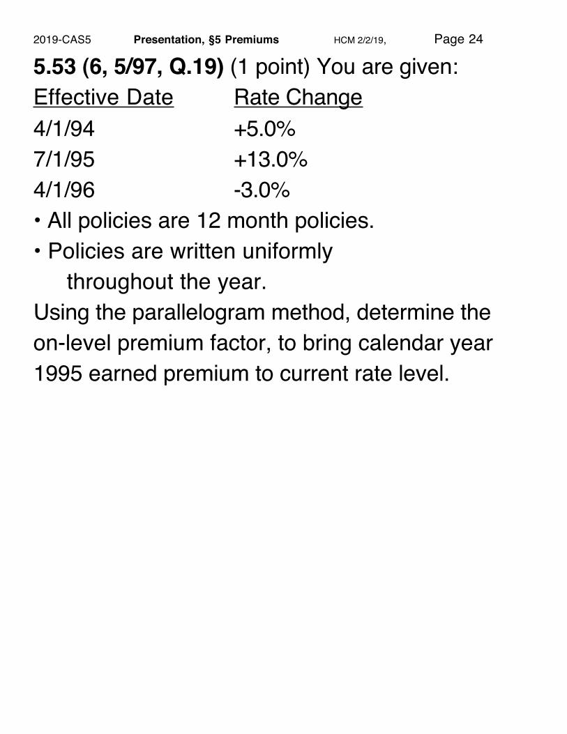
5.53 (6, 5/97, Q.19) (1 point) You are given:Effective Date Rate Change4/1/94 +5.0%7/1/95 +13.0%4/1/96 -3.0%• All policies are 12 month policies.• Policies are written uniformly
throughout the year.Using the parallelogram method, determine the on-level premium factor, to bring calendar year 1995 earned premium to current rate level.
2019-CAS5 Presentation, §5 Premiums HCM 2/2/19, Page 24

6, 5/97, Q.19. Effective Rate Level Rate LevelDate Change Factor (1/1/94 taken as = 1)1/1/94 1.0004/1/94 1.050 1.0507/1/95 1.130 1.18654/1/96 .970 1.1509
Area A = (1/4)2/2 = 1/32 = 0.03125.Area C = (1/2)2/2 = 1/8 = 0.125.Area B = 1 - (Area A + Area C) = 0.84375.
A
B
C
1/1/94 1/1/95 1/1/96
4/1/94 7/1/95
Average rate for calendar year 1995 earned prem. = (0.03125)(1) + (0.84375)(1.050) + (0.125)(1.1865) = 1.0655.
2019-CAS5 Presentation, §5 Premiums HCM 2/2/19, Page 25

On level Factor = Current Rate Level / Average Rate Level C.Y. 95 Earned Premium = 1.1509 / 1.0655 = 1.080.
Comment: Basic calculation you must know how to do! If for example, the 1995 Earned Premium were $100 million, then brought onto the current rate level 1995 Earned Premium would be:(1.080) ($100 million) = $108 million.
2019-CAS5 Presentation, §5 Premiums HCM 2/2/19, Page 26

Effective Date Rate Change4/1/94 +5.0%7/1/95 +13.0%4/1/96 -3.0%
5.54 (1 point) Using the information from 6, 5/97, Q.19, determine the on-level premium factor, in order to bring calendar year 1995 written premium to current rate level.
2019-CAS5 Presentation, §5 Premiums HCM 2/2/19, Page 27

5.54. The rate level index computation is the same.However, the diagram for written premium uses vertical lines rather than sloped lines.
B
1/1/94 1/1/95 1/1/96
4/1/94 7/1/95
A
Area A = Area B = 1/2.
Average rate for calendar year 1995 written prem. = (0.5)(1.050) + (0.5)(1.1865) = 1.11825.
On level Factor = Current Rate Level / Average Rate Level C.Y. 95 Written Premium = 1.1509 / 1.11825 = 1.029.
Comment: Many of use would not have to draw a diagram. One makes no use of the policy length.
2019-CAS5 Presentation, §5 Premiums HCM 2/2/19, Page 28

Effective Date Rate Change4/1/94 +5.0%7/1/95 +13.0%4/1/96 -3.0%
5.55 (1 point) Using the information from 6, 5/97, Q.19, except with 6-month policies, determine the on-level premium factor, in order to bring calendar year 1995 earned premium to current rate level.
2019-CAS5 Presentation, §5 Premiums HCM 2/2/19, Page 29

5.55. The rate level index computation is the same.However, in the diagram the lines have slope of1 / (1/2) = 2, rather than 1.
A
B
1/1/94 1/1/95 1/1/96
4/1/94 7/1/95
10/1/94
Area B = (1/2)(1/2)(1) = 1/4. Area A = 3/4.
Average rate for calendar year 1995 earned prem. = (3/4) (1.050) + (1/4) (1.1865) = 1.0841.On level Factor = Current Rate Level / Average Rate Level C.Y. 95 Earned Premium = 1.1509 / 1.0841 = 1.062.Comment: On level factor is less than when there were annual policies, since here more of the premium is earned under the new higher rates.See 6, 5/98, Q. 41.
2019-CAS5 Presentation, §5 Premiums HCM 2/2/19, Page 30
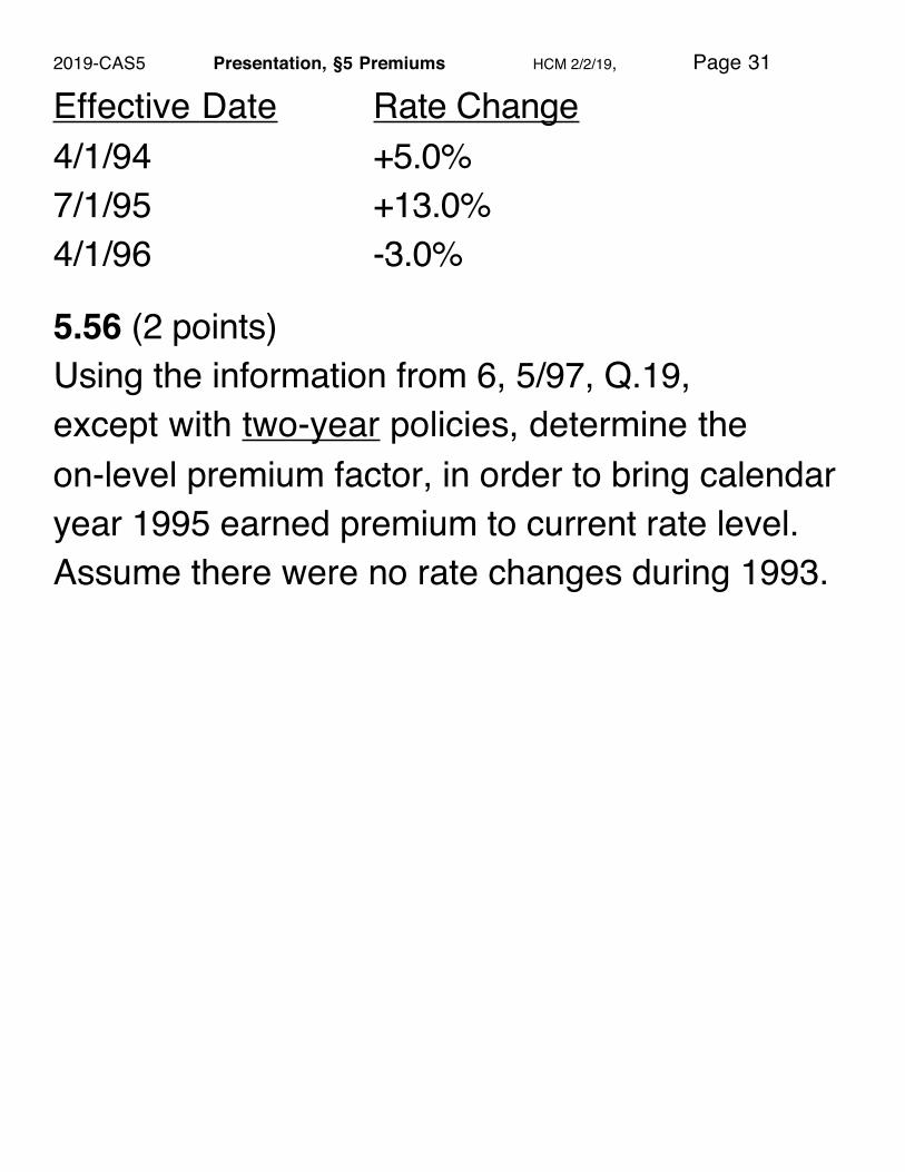
Effective Date Rate Change4/1/94 +5.0%7/1/95 +13.0%4/1/96 -3.0%
5.56 (2 points) Using the information from 6, 5/97, Q.19, except with two-year policies, determine the on-level premium factor, in order to bring calendar year 1995 earned premium to current rate level.Assume there were no rate changes during 1993.
2019-CAS5 Presentation, §5 Premiums HCM 2/2/19, Page 31

5.56. The rate level index computation is the same.However, in the diagram the lines have slope 1/2.
1/1/94 1/1/95 1/1/96 1/1/97
4/1/94
4/1/96
7/1/95
A
B
C
Area C = (1/2)(1/2)(1/4) = 1/16 = .0625.
Area A = difference of two triangles = (1/2)(5/4)(5/8) - (1/2)(1/4)(1/8) = 0.375.
Area B = 1 - 0.0625 - 0.375 = 0.5625.
Average rate for calendar year 1995 earned prem. = (0.375)(1) + (0.5625)(1.050) + (0.0625)(1.1865) = 1.0398.
On level Factor = 1.1509/1.0398 = 1.107.
Comment: See 5, 5/01, Q. 38.
2019-CAS5 Presentation, §5 Premiums HCM 2/2/19, Page 32
Effective Date Rate Change4/1/94 +5.0%7/1/95 +13.0%4/1/96 -3.0%
5.57 (1 point) Using the information from 6, 5/97, Q.19, determine the on-level premium factor, in order to bring Policy Year 1995 premium to the current rate level.
2019-CAS5 Presentation, §5 Premiums HCM 2/2/19, Page 33

5.57. The rate level index computation is the same.However, Policy Year 1995 (policies written during 1995) is represented by a parallelogram:
A B
7/1/95
1/1/95 1/1/96 1/1/977/1/96
Area A = Area B = 1/2.
Average rate for Policy Year 1995 premium = (0.5)(1.050) + (0.5)(1.1865) = 1.11825.
On level Factor = 1.1509/1.11825 = 1.029.
Comment: Many of us would not have to draw a diagram. It makes no difference in this case whether the premium is written or earned.
2019-CAS5 Presentation, §5 Premiums HCM 2/2/19, Page 34

page 161 Law Amendments:
When the Workers Compensation Law in a state is changed, either increasing or decreasing benefits paid to injured workers, or when the medical fee schedule is revised, actuaries estimate the average overall effect on losses.
Then usually a corresponding change is made to the rates based on the impact of this “law amendment.”
While rate changes normally apply to new and renewal business, often rate changes due to law amendments apply to all outstanding policies.
2019-CAS5 Presentation, §5 Premiums HCM 2/2/19, Page 35
For example, new higher benefits will be paid to workers injured in workplace accidents that occur on or after 7/1/10.
Therefore, Workers Compensation rates were increased by 10% on 7/1/10 in order to reflect this increase in benefits.
An annual policy written on 4/1/10, will cover accidents from 4/1/10 to 6/30/10, and from 7/1/10 to 3/31/11.
2019-CAS5 Presentation, §5 Premiums HCM 2/2/19, Page 36

The lower benefit level applies to the first group of accidents, while the new higher benefit level applies to the second group of accidents.
Therefore, the rates that were in effect when this policy was written on 4/1/10 are inadequate for the coverage provided from 7/1/10 to 3/31/11.
The rate for this policy will be increased mid-term on 7/1/10. The lower rate will apply to the first 1/4 of the policy period, and the new higher rate will apply to last 3/4 of the policy period.
Thus this policy will pay (10%)(3/4) = 7.5% more due to the law amendment.
2019-CAS5 Presentation, §5 Premiums HCM 2/2/19, Page 37
This differs from an ordinary rate change. If an insurer changed its rates after 4/1/10 for other than a law amendment, this policy would continue to use the rates in effect on 4/1/10.
⇒ Determining on-level factors for rate changes due to law amendments is somewhat different.
The law amendment rate change on all outstanding policies is represented by a vertical line.
2019-CAS5 Presentation, §5 Premiums HCM 2/2/19, Page 38

5.80b (5, 5/04, Q.31b) (2 points) Given the following information, answer the questions below. Show all work. • Policies are written uniformly throughout the year.• Policies have a term of 12 months.• The law amendment change affects all policies in
force. Assume the following rate changes: • Experience rate change on October 1, 2001 = +7%• Experience rate change on July 1, 2002 = +10%• Law amendment change on July 1, 2003 = -5% Calculate the factor needed to adjust policy year 2002 earned premium to current level.
2019-CAS5 Presentation, §5 Premiums HCM 2/2/19, Page 39

5, 5/04, Q.31b. Assume the rate level prior to 10/1/01 is 1.Policy Year 2002 earned premiums:
1/1/02 1/1/037/1/02
1/1/047/1/0310/1/01
A B
C
Area Rate LevelArea A 1/2 1.07Area B 1/2 - 1/8 = 3/8 (1.07)(1.1) = 1.177Area C 1/8 (1.07)(1.1)(0.95) = 1.118Average rate level for Policy Year 2002 earned premiums:(1.07) (1/2) + (1.177) (3/8) + (1.118) (1/8) = 1.116.Current rate level: (1.07) (1.1) (0.95) = 1.118.On-Level Factor: 1.118 / 1.116 = 1.002.
2019-CAS5 Presentation, §5 Premiums HCM 2/2/19, Page 40

Page 166 Premium Trend:
For some lines of insurance, even if the rate manual is kept the same, premiums will increase due to inflation.
For example, for Workers Compensation, even if the insured workers stay the same, the average weekly wages will increase with inflation, increasing payrolls, in turn increasing premiums.
For Homeowners Insurance, even if the set of insured homes remains constant, the value of insured homes will (usually) increase with inflation, in turn increasing premiums.
Even lines of insurance not affected by inflation can have their average premiums increase.
2019-CAS5 Presentation, §5 Premiums HCM 2/2/19, Page 41

When computing loss ratios for use in a rate indication, we would want to adjust both the numerator, losses, and the denominator, premiums, for the same effects. The changes in losses over time will be adjusted for via loss trend.
The corresponding changes in premiums over time will be adjusted for via premium trend. We will discuss the “one-step” and “two-step” methods.
We need to put the average premiums in the trend series on the same level.
If a change has a one time effect on premium level, one should make a direct adjustment. If a change occurs over time, then premium trend may be more appropriate.
2019-CAS5 Presentation, §5 Premiums HCM 2/2/19, Page 42

Written Premium Trend Series Example:
You are performing a rate indication, with a proposed effective date of January 1, 2008.
The proposed rates will be in effect for one year.12 month policies are written.
2019-CAS5 Presentation, §5 Premiums HCM 2/2/19, Page 43

You have the following data on premiums written, that is already adjusted for one-time, abrupt and measurable changes such as rate changes:
Ending Quarterly Average Written AnnualDate Premium at Current Rate Level Change
9/31/02 39312/31/02 3953/31/03 3966/30/03 3979/30/03 402 2.3%12/31/03 405 2.5%3/31/04 403 1.8%6/30/04 401 1.0%9/30/04 398 -1.0%12/31/04 399 -1.5%3/31/05 400 -0.7%6/30/05 404 0.7%9/30/05 409 2.8%12/31/05 413 3.5%3/31/06 416 4.0%6/30/06 415 2.7%9/30/06 413 1.0%12/31/06 417 1.0%3/31/07 416 0.0%6/30/07 418 0.7%
2019-CAS5 Presentation, §5 Premiums HCM 2/2/19, Page 44

You also have premiums and losses by Calendar/Accident Year:
Calendar Average Earned Incurred LossAccident Earned Prem. Premiums Losses Ratio
Year at Current at Current Developed Rate Level Rate Level to Ultimate
2002 392.11 5,234,501 4,346,582 83.0%2003 398.72 6,528,923 4,234,733 64.9%2004 401.04 6,030,067 4,863,410 80.7%2005 403.37 5,810,650 3,989,632 68.7%2006 413.93 5,620,354 3,689,457 65.6%
2019-CAS5 Presentation, §5 Premiums HCM 2/2/19, Page 45

A 3% annual loss trend has been selected.Using the simpler one-piece premium trend method, a 1% annual premium trend is selected. Determine the projected loss ratio for each calendar/accident year.
For policies to be written from 1/1/08 to 12/31/08, the average date of writing is 7/1/08, and the average accident date is 6 months later, or 1/1/09.
The loss trend factors are computed as follows:Accident Average Loss Trend Annual Loss Trend
Year Acc. Date Period Loss Trend Factor2002 7/1/02 6.5 years 3.0% 1.2122003 7/1/03 5.5 years 3.0% 1.1772004 7/1/04 4.5 years 3.0% 1.1422005 7/1/05 3.5 years 3.0% 1.1092006 7/1/06 2.5 years 3.0% 1.077
For example, 1.032.5 = 1.077.
2019-CAS5 Presentation, §5 Premiums HCM 2/2/19, Page 46

Calendar Year 2002 earned premiums, have an average data of earning of 7/1/02, and an average date of writing 6 months earlier, or 1/1/02.
We trend to an average date of writing of 7/1/08.
The one-step premium trend factors to be applied to earned premiums are computed as follows:
Calendar Average Premium Annual PremiumYear Written Trend Premium Trend
Date Period Trend Factor2002 1/1/02 6.5 years 1.0% 1.0672003 1/1/03 5.5 years 1.0% 1.0562004 1/1/04 4.5 years 1.0% 1.0462005 1/1/05 3.5 years 1.0% 1.0352006 1/1/06 2.5 years 1.0% 1.025
For example, 1.016.5 = 1.067.
2019-CAS5 Presentation, §5 Premiums HCM 2/2/19, Page 47
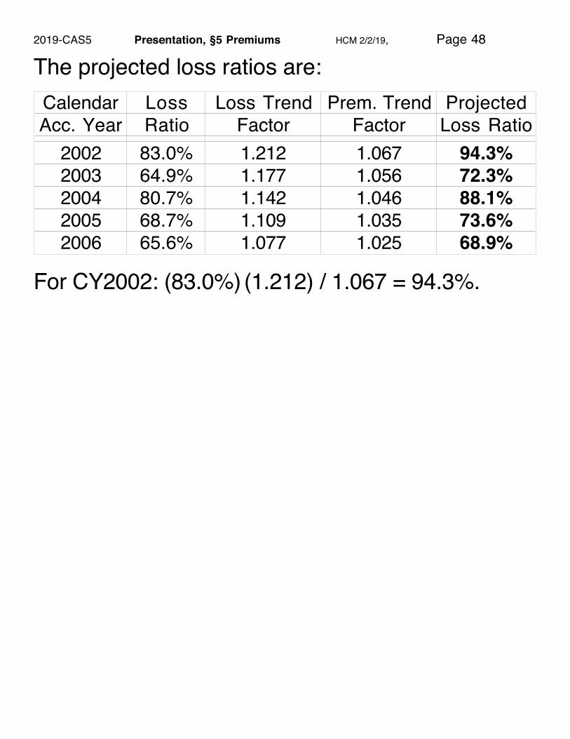
The projected loss ratios are:Calendar Loss Loss Trend Prem. Trend ProjectedAcc. Year Ratio Factor Factor Loss Ratio
2002 83.0% 1.212 1.067 94.3%2003 64.9% 1.177 1.056 72.3%2004 80.7% 1.142 1.046 88.1%2005 68.7% 1.109 1.035 73.6%2006 65.6% 1.077 1.025 68.9%
For CY2002: (83.0%) (1.212) / 1.067 = 94.3%.
2019-CAS5 Presentation, §5 Premiums HCM 2/2/19, Page 48

Rather than trying to compromise on the selection of a single long-term trend, the more complicated two-step trending method, as its first step, divides the latest average written premium at current rate level by the average earned premium at current rate level for each year in the experience period.
Step 1 Premium Trend Factor =
�
Latest Year Written Premium in Trend SeriesCalendar Year Earned Premium .
Where all premiums are at the current rate level.
2019-CAS5 Presentation, §5 Premiums HCM 2/2/19, Page 49

Using the two-piece premium trend method, in the second step a 1% annual premium trend is selected. Determine the projected loss ratio for each calendar/accident year.
Calendar Average Latest Step 1Year Earned Prem. Avg. W. P. Trend Factor2002 392.11 418 1.0662003 398.72 418 1.0482004 401.04 418 1.0422005 403.37 418 1.0362006 413.93 418 1.010
2019-CAS5 Presentation, §5 Premiums HCM 2/2/19, Page 50

In the two-piece premium trend method, for the second step an annual premium trend is selected.
The second step goes from the average date of the last point in the premium trend series to the midpoint of the proposed effective period of the new rates.
Based on the observed annual changes in the premium trend series, for example, a 1% annual premium trend is selected for the second step.
2019-CAS5 Presentation, §5 Premiums HCM 2/2/19, Page 51

The average written premium at current rate level for the quarter ending 6/30/07, the last period shown in the trend series, is given as 418. The quarter of written premiums ending 6/30/07 has an average data of writing of 5/15/07.
For policies to be written from 1/1/08 to 12/31/08, the average date of writing is 7/1/08.
CY06E.P.
Average WrittenDate 1/1/06
Average Date of Latest Value in the Trend Series 5/15/07
Eff. Date 1/1/08
Average WrittenDate 7/1/08
Step 1 Step 2
Annual Policies
2019-CAS5 Presentation, §5 Premiums HCM 2/2/19, Page 52

Thus the projection period is from 5/15/07 to 7/1/08, or 1.125 years.
The projection factor for premiums is: 1.011.125 = 1.011.
2019-CAS5 Presentation, §5 Premiums HCM 2/2/19, Page 53

The projected loss ratios are:
Cal. Loss Loss Step 1 Step 2 Proj.Acc. Ratio Trend Premium Premium Loss Year Factor Trend Trend Ratio
Factor Factor2002 83.0% 1.212 1.066 1.011 93.3%2003 64.9% 1.177 1.048 1.011 72.1%2004 80.7% 1.142 1.042 1.011 87.5%2005 68.7% 1.109 1.036 1.011 72.7%2006 65.6% 1.077 1.010 1.011 69.2%
For example:
�
(83.0%) (1.212)(1.066) (1.011)
= 93.3%.
2019-CAS5 Presentation, §5 Premiums HCM 2/2/19, Page 54

Use of Written Premium vs. Earned Premiumin order to compute Premium Trend:
Since these trends will apply to historical earned premium at current rate level, it makes some sense to evaluate trends based on shifts in average earned premium.
On the other hand, written premium data is more recent; premium for a given policy is not earned until well after it is written.
2019-CAS5 Presentation, §5 Premiums HCM 2/2/19, Page 55

5.39. (3 points) You are given the following information. Using a two-step trending procedure, answer the questions below. Show all work. • The premium trend series consists of quarterly values
from January 1, 2010 through December 31, 2013:1st Q 2010, 2nd Q 2010, ..., 3rd Q 2013, 4th Q 2013.
• Planned effective date is July 1, 2015.
• Rates are reviewed annually.
• Policies have a 6-month term.
• The trend will apply to calendar-accident year 2012 earned premium at current rate level.
a. (1 point) Calculate the beginning and ending dates for each of the Step 1 and Step 2 trend periods, assuming that the trend series consists of average written premium. b. (1 point) Calculate the beginning and ending dates for each of the Step 1 and Step 2 trend periods, assuming that the trend series consists of average earned premium. c. (1 point) Describe a situation when it may be more appropriate to use a two-step trending procedure, rather than a one-step trending procedure.
2019-CAS5 Presentation, §5 Premiums HCM 2/2/19, Page 56

5.39. a. Average date of earning CY12 Premiums is 7/1/12, with an average date of writing 3 months earlier (6 month policies) or 4/1/12.
The last average written premium in the series is for the quarter ending 12/31/13; this has average date of writing of 11/15/13.
Thus the first step goes from 4/1/12 to 11/15/13.
The average date of writing for the effective period is six months past 7/1/15 or 1/1/16.
�
⇒ The second step goes from 11/15/13 to 1/1/16.
2019-CAS5 Presentation, §5 Premiums HCM 2/2/19, Page 57
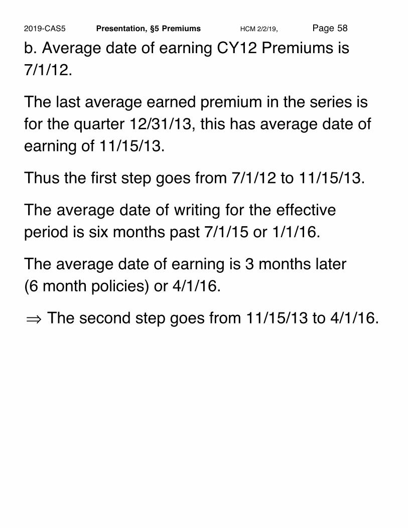
b. Average date of earning CY12 Premiums is 7/1/12.
The last average earned premium in the series is for the quarter 12/31/13, this has average date of earning of 11/15/13.
Thus the first step goes from 7/1/12 to 11/15/13.
The average date of writing for the effective period is six months past 7/1/15 or 1/1/16.
The average date of earning is 3 months later (6 month policies) or 4/1/16.
�
⇒ The second step goes from 11/15/13 to 4/1/16.
2019-CAS5 Presentation, §5 Premiums HCM 2/2/19, Page 58

6 Month Policies.
b. Earned Premium:Step 1: from 7/1/12 to 11/15/13.Step 2: from 11/15/13 to 4/1/16.
CY12E.P.
AverageWrittenDate 4/1/12
Average EarnedDate 7/1/12
Average Date of Latest Value in the Trend Series 11/15/13 Eff.
Date 7/1/15
Average WrittenDate 1/1/16
AverageEarnedDate 4/1/16
Written:Step 1 Step 2
Earned:Step 1 Step 2
a. Written Premium:Step 1: from 4/1/12 to 11/15/13.Step 2: from 11/15/13 to 1/1/16.
See Figure 5.28 in Basic Ratemaking.
2019-CAS5 Presentation, §5 Premiums HCM 2/2/19, Page 59

c. The two-step method would be more appropriate when there have been significantly different premium trends over the different periods of time involved.
The advantage of two-step trending is that it recognizes that there are situations where a single annual premium trend may not be appropriate for each year in the experience period.
Comment: Similar to 5, 5/04, Q.35.
2019-CAS5 Presentation, §5 Premiums HCM 2/2/19, Page 60