Career Women and the Durability of Marriage

Career Women and the Durability of Marriage∗

Andrew F. Newman† Claudia Olivetti‡

September 2015

Abstract

We study the relationship between divorce rates and female labor force attachment

in the US. Recent cross-sectional evidence from US states displays a robust negative

correlation between divorce and the rate of married female labor force participation.

We suggest that this pattern can be explained at least partly by increased bargaining

flexibility within two-earner as against one-earner households. Two-earner households

can use cash rather than less efficient in-kind or promised transfers to re-adjust intra-

household allocations when compensating for preference shocks or changes in outside

opportunities, rendering their marriages more durable. Using retrospective and longi-

tudinal data, we show that all else equal, there is a lower propensity to divorce among

families in which the wife is a “career woman,” i.e. has a higher labor force attach-

ment, though these families seem to display no lower incidence of marital difficulties.

We discuss policy implications of our findings.

Keywords: divorce, bargaining, nontransferable utility, marital instability, female labor

force participation

JEL codes: J12, D13, J21

1 Introduction

Many people believe that families with a working wife are more prone to divorce than those

with a stay-at-home wife. Indeed, as women entered the labor force in great numbers during

the 1960s and 1970s, divorce rates increased significantly, which helped to cement the notion

that marital instability and dissolution are costs of a gender-balanced workforce.1 A look

∗Thanks to Daron Acemoglu, Claudia Goldin, Georg Kirchsteiger, Victor-Rios-Rull, Dana Rotz, Alessan-dra Voena, Randy Wright and audiences at the NBER Summer Institute, Boston University, ECARES,Southampton, and the Barcelona Summer Forum for useful discussion. Deborah Goldschmidt providedoutstanding research assistance. We are grateful to our spouses for contributing to variation in the data.†Boston University and CEPR‡Boston College and NBER1An example in the popular press is Noer (2006). We discuss scholarship on the question below.

1

WV

AZ UT

TX

AL

NM

KY

ID

OK

NV

TNFLMS

GA

WA

AR

SC

OR

NY

MI

NC

IL

NJ

VA

COAK

PA

HIMO

OH

DE

MT

WY

CT

ME

MD

KS

MA

RI

NH

DC

WI

VT

MNNE

IA

NDSD

Correlation= -.5242

34

56

7D

ivorc

e R

ate

(per

1000 p

opula

tion)

0.60 0.65 0.70 0.75 0.80

LFP Married Women

LFP is from the American Community Survey 5-year sample- 2005-2009.Divorce rate is from the U.S. National Center for Health Statistics- National Vital Statistics Reports. We use the average over 2005-2009. Missing observations on divorce rate for CA, IN and LA. For GA, HI and MN, divorce rate used is from 2000.

LFP rates of married women and divorce rates by state - 2005-2009

Figure 1: Divorce and married women’s labor supply, ACS 2005-2009

at more current evidence, however, suggests that this view needs to be reconsidered. For

example, as displayed in Figure 1, there is actually a negative relationship between the

divorce rate and the rate of married female labor force participation (MFLP) across U.S.

states. This pattern is opposite to what would be expected if working wives were contributing

on net to marital fragility. What then has the conventional wisdom missed? Could it be

that working women are good for marriage?

Economic theory provides a simple answer. It predicts that households with two perma-

nent earners will behave differently from those with only one because of differences in the

degree of transferability among household members. An earner can compensate with money,

or what is the same thing, a balanced basket of market-procured and household-produced

goods, while a non-earner must compensate only with household-produced goods. Thus,

compared to a one-earner household with the same income, a two-earner household will be

better able to make the frequent adjustments to consumption needed to keep both partners

happy in the face of preference changes, new outside opportunities, or other vicissitudes. Un-

der mild assumptions about the distribution of these “shocks,” the result is a marriage for

the two earner household that is less likely to dissolve; more generally, this marital durability

is increasing in the equality of partners’ earnings.

In this paper, we illustrate the theoretical argument for this “transferability effect” and

then provide evidence that it is operative in US households. To that end, we show first that

2

the cross-state negative correlation in Figure 1 is robust to various controls, in particular

the state-level median age at first marriage and the mean level of female education, both

of which have been shown to be negatively correlated with divorce (Lehrer, 2008; Isen and

Stevenson, 2010; Rotz, 2011; Lehrer and Chen, 2013).2

We then turn to micro-level evidence, which lets us confront two challenges to empiri-

cal identification of the transferability effect. First, in some households, causality may be

running from the state of the marriage to the labor supply decision, rather than the other

way around. In particular, there may be households where the marriage is unstable, and the

woman is therefore working either as a precaution (divorce is expected and she is investing in

human capital or labor market contacts) or to compensate for losses in husband’s income.3

Such “remedial earners” would tend to generate a positive correlation between working and

divorce, obscuring the negative relation predicted by the transferability effect. Indeed, in

the conclusion we discuss how the presence of remedial earners may confound interpretation

of the cross-sectional evidence on female labor force participation and divorce and the policy

implications to be drawn.

We address this problem in two ways. First, we focus on “career women,” measured

variously, but basically defined as those who are in the labor force a substantial fraction of

the time both before and during marriage.4 Compared to remedial earners, career earners

have lower costs of generating cash and current incomes that are more closely tied to their

permanent incomes, both of which are attributes that facilitate the operation of the trans-

ferability mechanism. Second, we use panel data, particularly the distribution of earnings

within households, to follow couples over time and help tease out the remedial from the

career earners.

The second difficulty comes from possible selection effects – a woman’s propensity to have

a career may be correlated with other attributes that lead her to have a higher quality and

therefore more durable marriage. We have already mentioned age at marriage and education

as examples, but there could be unobserved ones as well, such as character traits or match

quality that are correlated with career orientation. We handle this concern by exploiting a

battery of quality-of-marriage questions in our data that allow us to assess whether career

women in fact select into better marriages.5

We find that all else equal, those couples in which the women are more attached to

2Age at marriage and education are obviously correlated with labor force participation, but could haveindependent effects on marital stability. Couples who are older when they marry may be more informed andtherefore make better choices. Education, particularly college, may reduce marital search costs.

3Much of the literature, especially outside economics, refers to marriages that are unmarked by strife,conflict, appeal to outside counseling and other indicators of low marriage quality as being highly “stable”;we shall follow suit and reserve the term “durable” for marriages that have a low probability of divorce.

4This is close to the notion of career woman as one who works regardless of marital status (e.g. Goldin,1995); in 2000, over 85% of single women 25 to 34 were working, while only 70% of married women were.

5Our information on both earnings and quality of marriage come from the Marital Instability over theLife Course panel, which follows married couples over a twenty-year span and records information aboutlabor force participation, earnings, and other economic and demographic characteristics, as well as a rich setof indicators of marital happiness.

3

the labor force are less likely to divorce. Moreover, female labor force attachment has the

strongest stabilizing effect in couples in which the woman earns close to 50% of family income.

However, we do not find that these families have lower rates of marital disagreement. Taken

together, our results suggest that it is the flexibility to accommodate disagreement, rather

than a reduction in its incidence, that is keeping two-career marriages together.

Literature

Existing explanations connecting divorce and MFLP are varied, but all suggest that MFLP

and divorce rates should covary. Most find causality running from MFLP to divorce rates:

career women are more independent and therefore willing to divorce, (Nock, 2001); the

incomes of husbands and wives are substitutes, making marriage between equals less valuable

(Becker, Landes, and Micael, 1977); there is increased marital conflict within career couples

(Mincer, 1985; Spitz and South, 1985), etc. As already mentioned in conjunction with

remedial earners, there is a possibility that causality runs the other way, and there is indeed a

significant set of papers that explore this possiblity. In the face of high divorce rates, married

women have increased incentives to invest in careers, as a kind of self insurance (Greene and

Quester, 1982; Johnson and Skinner, 1986). Relatedly, if divorce is likely, women spend less

of their adult life in marriage, which reduces the returns from specializing in the home, and

increases the incentives to invest in labor marketable skills (Stevenson, 2007). Finally, some

authors have suggested that the two trends reflect a spurious correlation: improvements

in home production technology, which both lowers the opportunity cost of working and

reduces the value of a marriage, have contributed to increased MFLP and to increases in

divorce (Ogburn and Nimkoff, 1955; Greenwood and Guner, 2004). In recent work, Stevenson

and Wolfers (2007) suggest that other technological factors, such as the contraceptive pill,

and changes in the wage structure, that have been found to be important determinant for

the increase in labor force participation of married women might also be responsible for a

concurrent increase in divorce rates.6

In addition to re-examining the relationship between divorce and MFLP, this paper con-

tributes to a literature that seeks to distinguish empirically the effects of varying degrees

of transferability within households and other institutions. It has long been understood

theoretically that the non- or imperfectly-transferable-utility case differs radically from the

transferable-utility one in terms of both predicted behavior (intra-household allocations,

choice of organizational design in firms, sorting patterns, or investment behavior) and wel-

fare (Becker, 1973; Legros-Newman 1996, 2007; Peters and Siow, 2002). There has been

rather less work that derives practically testable implications of these differences (e.g., Cher-

chye, deRock and Vermuelen, 2015) or that implements them empirically (Udry, 1996).

6Rasul (2006) suggests that changes in divorce law would have led to temporary increases in divorce thatwould then have fallen back to trend levels, which have in fact been falling over the past twenty years; seealso Wolfers (2006). It is not clear whether this “pipeline” effect can account for the whole trend over fortyyears, and in any case it makes no connection between divorce and MFLP.

4

The rest of the paper proceeds as follows: in the next section we present a simple model

of the transferability effect. Section 3 begins our empirical analysis with aggregate as well as

retrospective micro-level evidence that broadly supports the view that career women enhance

marital durability. The main empirical analysis based on longitudinal data is presented in

Section 4. Section 5 offers concluding remarks, with some discussion of trends and policy

implications.

2 Conceptual Framework

The purpose of this section is to provide a simple reduced form model that isolates the

transferability effect in order to show how it affects marriage durability. In the empirical

section we will, of course, have to take account of other effects (some of which we have

already mentioned) that may effect durability but whose logic is already well established in

the literature.

We employ the standard household bargaining framework in which the two decision

makers derive utility from private goods and a local public good that is enjoyed if and only if

they remain together. Assume that preferences can be represented by an additively separable

utility of the form ui(c)+φ, where c is a vector of private good consumption and φ represents

the utility of “local public goods” (LPG) derived from the marriage (companionship, children,

possible scale economies in housing or other private goods), representing the net benefit of

remaining married.7 Assume that preferences are monotone and that the indirect utilities

corresponding to u(c)i are linear in income.8 If the couple were to divorce, they would

each obtain an autarky payoff represented by the indirect utilities (v, I − v), where v is the

monetary earnings of one partner, and I − v that of the other.

Money facilitates transferability. There are several possible reasons for this. One is

that money enables the purchases of balanced bundles of consumption goods that may

be transferred between partners. In-kind transfers are less efficient means of transferring

utility. The second reason, inspired by contract theory, is that money can be transferred

now, whereas in-kind payments may have to be transferred in the future. The monetary

transfers are thus less subject to moral hazard and other commitment problems than are

other means of intrahousehold transfers. Third, money enables an aggrieved party to directly

purchase a suitable good that may compensate for a loss of LPG utility rather than engaging

in costly bargaining to get the partner to do so.

7Though φ might depend on income in some of these interpretations, we suppress that dependence here,as we control for household income in both the theoretical and empirical analyses.

8There is a significant literature (e.g. Bergstrom and Varian, 1985) that studies restrictions on preferenceslead to such utility functions and to transferable utility possibility frontiers assuming that there is frictionlesstrade between the partners in all goods. It is worth emphasizing that we are not so much concerned with thisissue as with money’s role in diminishing frictions such as transaction costs or moral hazard that would turna linear frontier into a nonlinear one; our basic point would remain valid even if preferences did not satisfythe Bergstrom-Varian restrictions, though the computations would naturally be rather more complex.

5

Thus, utility transfers can be made one-for-one transfers with money. Beyond the limit

of monetary means, utility transfers are accomplished less efficiently: along the frontier, the

utility given up by one partner exceeds that gained by the other. Thus when one partner’s

utility is less than φ, the slope of the frontier is less than 1 in magnitude, while above φ+ I,

the slope exceeds one. We assume these non-monetary means of making utility transfers are

equally effective on the margin, given their level, for each partner: the frontier is symmetric

about the 45-line.

Figure 2 illustrates the basic logic. Two households, 1 and 2, with equal incomes I and

equal initial realizations φ of the payoffs from the LPG, share a utility possibility frontier

(W0). There is perfect transferability achieved by sharing earned income (so that the indirect

utilities are given by (y1 +φ, y2 +φ), where yi is the income used by by partner i to purchase

private consumption. The frontier illustrates the extreme case of no transferability beyond

the household earned income I. The households differ only in the way in which earned

income is initially distributed. Household 1 has one earner: this is reflected by the utility

distribution that would occur if the household were to divorce, which is represented by the

autarky point A1. Household 2 has two (equal) earners, with autarky payoffs represented

by A2. Suppose that the households have reached an equilibrium allocation of private goods

— we make no particular assumptions about the bargaining protocol they use except that

it does lead them to some point on their Pareto frontier.

Now let each partner experience a “shock” to the payoff from the LPG, indicated by the

dashed arrow 1 in the diagram. This could represent such things as a change in how they feel

about each other, the unexpected pleasure (or stress) from an additional child, or since the

LPG simply represents the partners’ net benefits of being married to each other, a change

in outside opportunities. Following the shocks, there is a new utility possibility frontier W1.

Shocks could be positive or negative; in this case W1 reflects a mild negative shock for partner

1 and a distressingly large one for partner 2. The partners may be induced to renegotiate

the allocation of private goods following the change in LPG. As long as the autarky payoff

vector is Pareto dominated by some point on the frontier, the couple will remain married

and settle on a payoff allocation on the new frontier. But should the autarky payoff now lie

“outside” the frontier, there are now no realizable net gains from trade, and the couple will

divorce. In the figure, the one-earner household 1 divorces, but following the same shock,

the two-earner household 2 remains married.

There are of course shock realizations that could result in divorce for Household 2 but not

for Household 1 (shock 2 in the figure). But under mild restrictions on the distribution of

shock values (roughly, that large ones are less probable than small ones), this is a less likely

outcome, and the result is that the 2-earner household’s marriage is more durable. Though

our focus in the empirical analysis is on the difference between egalitarian households like the

two-earner Household 2, and rather less egalitarian ones like Household 1, it turns out that

these same properties of shock distributions imply that the relationship between earnings

equality and marriage durability is monotonically increasing.

To be a bit more formal, represent the household utility possibility frontier by (x,W (x)),

6

W0

W1

U2

U1 0

A2

W2 A1

1

2

I I+ϕ

Figure 2: Bargaining sets before (W0) and after (W1,W2) shocks to the LPG of one- andtwo-earner households. At W1 Household 1 divorces, Household 2 remains married. The lesslikely large shock leading to W2 has the opposite effect.

where W (x) is a continuous, strictly decreasing (therefore a.e.-differentiable), self-inverse

function on R, with W (x) = I + 2φ− x for x ∈ [φ, φ+ I]. Elsewhere,

0 ≥ W ′(x) > −1 a.e. on (−∞, φ) and W ′(x) < −1 a.e. on (I + φ,∞).

The self-inverse property W (W (x)) ≡ x captures the symmetry of the partners in their

(ex-ante) tastes for the LPG and for their ability to make utility transfers beyond those

effectuated with monetary earnings. One partner earns v, the other earns u = I − v, where

0 ≤ v ≤ I. Thus v = I/2 is the egalitarian two-earner household, and v = 0 (or v = I) is

the one-earner household.

The value of the local public good is subject to a shock for each partner, after which

they renegotiate the intra-household allocation. Shocks are drawn independently from the

same distribution F (·) with support (−∞,∞) and density f(·). The density f is log concave,

though this can be relaxed.9

9The density f is log-concave if log f is concave; this implies f(x)f(y)− f(x− δ)f(y + δ) ≥ 0 for x < yand δ > 0, among other things; many commonly used distributions (including the uniform, normal, logistic,and Laplace) have log-concave densities. See e.g., Bagnoli and Bergstrom (2005).

7

If the household divorces, each member gets an autarky payoff equal to the indirect utility of earnings, i.e., the autarky payoff is (v, u). It is convenient to think of the shocks as being added to the autarky payoffs rather than subtracted from the value of the public good. As long as the shocks (ε, η) added to the autarky payoffs remain inside the frontier, that is, u+η ≤ W (v+ε), the marriage continues. Given ε, this happens with probability F (W (v + ε) − u), and the marriage’s durability – the probability that it stays together – is then

D(v) =

∫ ∞−∞

f(ε)F (W (ε+ v)− u)dε

One special case is worth noting. When W (x) = I + 2φ − x everywhere (full transfer-

ability), then the argument of F (·) is just 2φ− ε, i.e. the distribution of earnings within the

household, as well as their aggregate level, are irrelevant.

We now state and prove the main theoretical result.

Proposition 1 Suppose the household has income I and the value of local public good is φ

for each partner. Assume

(1) The household utility possibility frontier is symmetric, transferable on [I, I + φ] and

imperfectly transferable outside of [I, I + φ];

(2) Preference shocks are i.i.d. with log-concave density.

Then the durability of marriage is increasing in the equality of household earnings.

Proof We show that D(·) is increasing below I/2 and decreasing above I/2. Now,

D′(v) =

∫ ∞−∞

f(ε)f(W (ε+ v)− u)(W ′(ε+ v) + 1)dε.

Make the change of variable x ≡ ε+ v; then

D′(v) =

∫ ∞−∞

f(x− v)f(W (x)− u)(W ′(x) + 1)dx.

Since W ′(x) + 1 = 0 for x ∈ (φ, φ+ I),

D′(v) =

∫ φ

−∞f(x− v)f(W (x)− u)(W ′(x) + 1)dx+

∫ ∞φ+I

f(x− v)f(W (x)− u)(W ′(x) + 1)dx.

Use the change of variable x̂ = W (x) in the second term, and note that W (x̂) = x, x = φ+I

implies x̂ = φ, and x→∞ implies x̂→ −∞, to rewrite this as

D′(v) =

∫ φ

−∞[f(x− v)f(W (x)− u)− f(x− u)f(W (x)− v)](W ′(x) + 1)dx. (1)

Since x−min{u, v} < W (x)−max{u, v} on (−∞, φ] and (x−v)−(x−u) = (W−v)−(W−u),

log-concavity of f implies f(x− v)f(W (x)− u)− f(x− u)f(W (x)− v) ≥ 0 iff v ≤ u, with

8

strict inequality on a non-null set. Moreover, W ′(x) + 1 > 0 a.e. on (−∞, φ]. Thus, D′ > 0

when v < u and D′ < 0 when v > u, as claimed. 2

Remark 1. Symmetry is a natural benchmark. But in the asymmetric case in which

one partner values the marriage more than the other, durability will tend to be maximized

at a point where that partner has a higher monetary income. A leading example of such

preferences is when one partner dislikes being in the labor force relative to remaining in

the home. If marriage allows this partner to remain at home, the distribution of earnings

is opposite to what it needs to be to maximize durability, reinforcing our contention that

marriages in equitable two-career households are the most durable.

Remark 2. Although reasonably innocuous, log concavity is unnecessarily restrictive,

largely because it imposes structure on the “good” shocks that do not affect durability;

only the “bad” shocks matter. If the frontier is concave, it is enough that the density f

is decreasing on [φ,∞): among shocks that that are big enough to completely wipe out

a partner’s gains to marriage, larger shocks are less likely than smaller ones.Details are in

Appendix 2.

Remark 3. It is not necessary that autarky payoffs equal the (indirect utility of) within-

marriage earnings: what matters is that the autarky payoffs corresponding to equal earnings

are equal and that the difference in the autarky payoffs is monotonically increasing in the

earnings difference.

Remark 4. The result is not merely about the role of inequality; transferability is also

important. Indeed, if the autarky frontier T (and therefore W (x) on [φ, 2I + φ]) is concave

“enough,” it is easy to find examples where D′ = 0 when v = u, but D′′ > 0 there, so

that equality is a (local) minimum for durability. This is obvious if one thinks of the case

of strictly non-transferable utility; then conditional on a shock for one partner smaller than

φ (else the marriage breaks up), it is clear that moving the autarky point toward equal

payoffs minimizes the chance that the other partner’s shock is small enough to preserve the

marriage. Thus it is appropriate to interpret the result as saying that equality of earnings is

good for marriage not because equality per se is durability maximizing, but because equality

maximizes transferability within the household for the most relevant shock distributions.

3 The relationship between married women’s labor force

participation and divorce

We now show that the negative relationship between the divorce and MFLP depicted in

Figure 1 is robust to a number of state-level controls.10 Table 1 presents the results, where

we progressively add other factors.11 Column 1 reports the regression coefficient for the basic

10In an earlier version of the paper we showed that the same negative correlation across US states isobserved based on Census 2000 data.

11See Data Appendix for a detailed discussion of data sources and variable definitions. In all the regressionsthe state level variables are population-weighted.

9

regression (this corresponds to the correlation coefficient reported in Figure 1). According to

our estimate, which is significant at the 1% level, a state that has a 10% higher MFLP has

0.86 fewer divorces per 1000 people per year. Since the average divorce rate is 3.6 per 1,000,

this corresponds to a 25% reduction in the divorce rate. Column 2 adds the marriage rate.

The coefficient is positive, reflecting the greater per capita stock of marriages that can end in

divorce. Nevertheless, the negative correlation between divorce and labor force participation

is unaffected, so it is not driven by hypothetically lower marriage rates in states where more

women work.

A number of state-level characteristics might be driving this correlation. For example,

it has been shown that more educated women are less likely to divorce than less educated

women (Martin, 2005; Isen and Stevenson, 2010), as well as more likely to work, so that

as the average level of female education increases, the divorce rate should fall. In addition,

Rotz (2013) shows that age at first marriage has an independent negative effect on divorce.

However, controlling for the mean level of female education in the state and for age at first

marriage, the negative correlation between divorce and MFLP survives (column 3). MFLP,

marriage rate, age at first marriage and education are all important: taken together they

can explain 61 percent of the overall cross-state variation in divorce rates.

Our results are robust to the inclusion of a number of additional explanatory variables.

For example, it has been suggested that higher male income inequality increases the option

value of a searching for a mate, which could result in higher quality marriages (Loughran,

2002; Gould and Paserman, 2003). Another possibility is that lower occupational sex-

segregation increases the meeting rate with opposite sex co-workers, which could lead to

lower marital durability (McKinnish, 2004). Moreover, there is evidence that women in uni-

lateral divorce states with common property laws are less likely to work and more likely to

divorce (Voena 2014). As shown in column 4, the correlation between divorce and MFLP

retains its sign and significance even after having controlled for all these factors.12

The evidence across US states displays a negative correlation between the fraction of

married women who work in a state and the prevalence of divorce there. While this is

certainly consistent with the prediction of our model, the correlation could be driven by

other factors. To identify the transferability effect requires that we turn to micro-level data.

In keeping with our theoretical analysis, we want to use an indicator of a woman’s

attachment to the labor force during marriage, rather than her current labor supply. This

approach is essential if we are to examine our hypothesis correctly. Not only is the theory

best interpreted in terms of transfers of permanent rather than transitory income, but there is

a crucial inference problem that arises in cross-section or short-panel data. In a cross-section

of women we might observe that working women are more likely to be divorced, but this

could simply reflect their need to make up for lost income from the break up. Similarly, in a

12Column 5 omits Nevada, which leaves the results unchanged. We have experimented with alternativemeasures of married women labor force participation, such as full- and part-time participation, labor forceparticipation of white women and labor force participation of 25-54 year old women. For all specificationswe obtain results similar to the ones reported here.

10

short panel in which data are collected at only two dates, women who happen to anticipate a

divorce in the near future may be (temporarily) working at the first date and be divorced at

the second date. This could make it appear as though working women contribute to marital

fragility when in fact it reflects precautionary or remedial working. We are led therefore to

examine evidence from retrospective and, more important, longitudinal data.

Evidence based on retrospective data

We first use the 2008 Survey of Income and Program Participation (SIPP). This is a large

cross-section that has retrospective information on both work history (from Topical Module

1) and marriage history (from Topical Module 2).13 This data set has been prominently used

in this literature. For example, Isen and Stevenson (2010) use the retrospective information

on marital status to document trends in marriage formation and dissolution by race and

education over the past few decades. We add to their work by showing that, all else equal, a

“career” woman, i.e. with higher labor force attachment, has a lower propensity to divorce.

Our measure of labor force attachment during marriage is obtained by matching informa-

tion on labor market interruptions (from the employment history module) with information

on marriage spells (from the marital history module). Unfortunately, the questionnaire does

not give any indication of when the time off was taken, making it difficult to determine

whether a spell of non-employment occurred before, during, or after marriage, especially for

women whose first marriage dissolved before the survey. In addition, it is not clear whether

time off is considered separately from time off spent caregiving, and one needs to avoid

double-counting any time off. Because of this limitation of the data, we exploit informa-

tion on start and end dates of employment and marriage to construct a binary indicator

of whether a woman worked at all during her first marriage rather than more continuous

estimates of time spent working. This indicator takes a value of one if a woman started,

but didn’t stop, working before entering her first marriage, or if she first started working

after her first marriage started but before it ended (if it ended). It takes a value of zero if

she never worked; if she worked, but stopped working before her first marriage began; if she

started working only after her first marriage ended; or if her time caregiving spanned her

entire marriage. While this indicator does not capture the intensity of labor force attachment

during marriage, it does not rely on ‘ad hoc’ assumptions and is relatively clean.

At the same time it seems to capture the essence of being a ‘career’ woman. As shown

in Table A.3, our measure of work during marriage is positively correlated with age at first

marriage and at first birth, conditional on having children during first marriage, full-time

work and earnings (three alternative measures). ‘Career’ women are also more likely to have

a college or post-graduate degree, and to work in professional occupations.14

13See Appendix 1 for details.14Details about the construction of this variable can be find in section 5. We have also experimented with

alternative classifications. For example, we exploit all the available information on spells of non-employmentto refine our measure of labor force attachment. In this case our binary indicator equals one if a woman

11

We consider the sample of all women age 25-54, who are either in their first or second

marriage, or separated/divorced by the time of the survey.15 We include in our sample

only marriages that occurred in the 1990s or later. This is to minimize the bias due to the

retrospective nature of our data and to make our sample as comparable as possible to that

used in our state cross section. Summary statistics for the sample are reported in appendix

table 2. Women in our sample are 37 years old, on average, 81% of then are white, 11%

are blacks and 6% asian, 57% of the women in our sample have at least a four-year college

degree. The entered their first marriage when they were about 26 years old, on average, and

they have, on average, 1.94 children. Approximately thirty percent of all marriages in our

sample end in divorce; of these, the average marriage lasts five years, and 60% of divorces

occur by year 5.

We report the regression results in Table 2. The dependent variable is the probability

that a marriage dissolves by year 5. Column 1 shows that there is a negative and significant

correlation between whether a woman worked during her marriage and the probability of

a dissolution within the first 5 years of marriage.16 According to our estimate, a marriage

involving a career women is approximately 8 percentage points less likely to end in divorce

within the first 5 years. Since the average rate of divorce by year 5 is 18%, this reduction is

sizable (corresponding to 45% of the probability to divorce within the first 5 years of (first)

marriage). We worry that this finding might be driven by education. College educated

women are both more likely to work and less likely to divorce than women with lower levels

of education. Thus in column 2 we add a high education dummy that equals one for women

with a bachelors degree or higher and 0 otherwise. We find that the coefficient on our labor

attachment variable does not change substantially. Its magnitude drops from 0.08 in column

1 to approximately 0.06 in column 2. Consistent with the results reported by Isen and

Stevenson (2010) we find that divorce rates are lower, by approximately 4 percentage points,

for highly educated women. As shown in column 3, the negative association between divorce

and labor force attachment stands even after having added controls for race, age at first

marriage, marriage duration, an indicator of whether the couple had a child under the age

of 6, an indicator of property division laws in the current state of residence which is equal to

one if the states has community property (that is, is characterized by an equal distribution of

property upon divorce independent on title ownership) and a dummy equal to one if the state

of residence has unilateral divorce (as opposed to mutual consent).17 Consistent with Rotz

(2013) we find a strong negative correlation between age at marriage and divorce. Consistent

worked 1 to 100% of her first marriage and zero otherwise. The results obtained under this alternativeclassification scheme are basically identical to those reported in the paper.

15Restricting the data analysis to first marriages is a common assumption when studying marital outcomes.See for example Isen and Stevenson (2010).

16We also ran regressions looking at the probability of dissolution by year 7 and 10 as well as a Coxproportional hazard model and found very similar results.

17Obviously assigning divorce law by current state of residence rather than state of residence at timemarriage or divorce is not ideal. However, SIPP does not report this information so this is the most we cando.

12

with Isen and Stevenson (2010) we find that blacks are more likely to divorce. Finally, we

find that women who reside in states with community property (who, except for Louisiana,

also have unilateral divorce) are less likely to divorce, while residing in a unilateral divorce

state does not seem to affect the probability of divorce one way or another. This is consistent

with findings by Wolfers (2006). The overall finding is that all else equal, a marriage to a

career woman is about 6 percentage points less likely to end in divorce, which corresponds

to a 34% decline in the 5-year divorce probability.

Although the SIPP provides further evidence of a negative correlation between labor

force attachment and divorce, it is not ideal for our purposes. The measure of labor force

attachment during marriage that can be constructed from SIPP is very noisy. And although

it includes information on the current spouse, any information about past spouses and mar-

riages to them is absent for women who divorced before the survey year. Finally, it lacks

information pertinent to identifying the transferability effect, such as the share of household

income earned by the wife or the quality of the match.

The Marital Instability over the Life Course (MILC) data set discussed in the next

section provides a relatively long panel of marriages, thus mitigating the issue of measuring

attachment and pre-divorce characteristics. It also contains a rich battery of qualitative

questions on marital happiness or marital problems that can be used to tease out alternative

explanations.

4 Longitudinal Analysis

The starting point of this exercise is to construct marital and employment histories for a

cohort of married couples and study how, all else equal, wives’ employment status or change

thereof affect the stability of the couple’s marriage over time. This requires the use of a panel

data set where we can follow the couple over a reasonable period of time and distinguish

women who are temporarily working from those who are permanently working (hence labor

force attachment) as well as observe whether the marriage ultimately ends in divorce.

We draw on the Marital Instability over the Life Course (MILC) data set that follows

married couples over a 20-year span.18 This data set is very useful for our purposes as it

was designed in order to examine the causes of marital instability of a group of married

individuals.19 It consists of a national probability sample of 2,034 married men and women

under 55 who were interviewed by telephone for the first time in the fall of 1980. They were

re-interviewed five times, which generated a total of six waves of data, collected in 1980,

18Booth, Johnson, Amato, and Rogers (2003), ICPSR Study No.: 3812: Marital Instability Over the LifeCourse [United States]: A Six-Wave Panel Study, 1980, 1983, 1988, 1992-1994, 1997, 2000.

19The paper most closely related to our study is Booth, Johnson, White and Edwards (1984). In thispaper the first two waves of the survey are used to analyze the impact of wives’ employment on maritalinstability (broadly defined as the set of all divorce-related activities: from thinking about it to filing forseparation/divorce). They find a positive but small effect of a wife’s hours of market work on maritalinstability. But as suggested above, this is likely the result of the confounding effects that a short panelcannot distinguish.

13

1983, 1988, 1992-1994, 1997 and 2000. The characteristics of the sample were compared

with estimates made by the U.S. Census Bureau, and the 1980 sample was found to be

nationally representative with respect to age, race, household size, presence of children,

region, and female participation to the labor market.

We select only couples who are in their first marriages in 1980 and in which both spouses

are older than 18. We obtain a sample of 827 marriages of which 627 are still intact in year

2000, that is, 24% of the couples in our sample divorced by the end of the survey. Summary

statistics for the sample are reported in Table A.4.

In order to investigate our hypotheses we run a linear probability model where the de-

pendent variable is equal to one if the couple divorced any time between 1980 and 1997 and

is equal to zero otherwise.

The main dependent variable in our benchmark specification HighAttachment is an

indicator function equal to one if the wife was highly attached to the labor force over this

period (definitions provided below). We also include the same set of controls included in

the regressions discussed in Table 1 and 2.20 These include, among others, age at marriage,

marriage duration, number of children and, for both spouses, race, educational attainment

and its change over the course of the current marriage. We also include average family

income and an indicator of intra-household ’earnings equality’ over the period.

Since we follow a set of couples over time we need to update all the relevant time-varying

variables. Specifically, wife’s time spent working, husband’s full time work participation,

years of marriage, and the number of children are updated. The main difficulty, however,

is in updating the information about amount of wife’s time spent working. This is done by

combining the information about whether the wife worked after marriage and in between

each round of the survey.21

Our baseline labor attachment construct is a dummy equal to 1 if a wife worked more

than 75% of the time since marriage, and zero otherwise. Approximately 68% of the wives

in our sample are classified as being high labor force attachment according to this definition.

As shown in Table A5, “High Attachment” women are more likely to have a college degree

and to earn more. However, their husbands are not statistically different, except for having

had a working mom while growing up.

As an alternative we use Career = 1 if a respondent said that “pretty important” or “very

important” reasons for wife working were having a career, for a sense of accomplishment, for

contact with other people and for financial independence. According to this definition 64%

of wives in our sample are career women. The correlation between “high attachment” and

“Career” is relatively high (0.6, p-value=0.001).

20In this case we cannot control for state-level divorce law. This is because the information on state ofresidence is only recorded in 1997. However, by 1997 most of the ever divorced couples in our sample havealready split.

21The main construct excludes wife’s labor force participation before marriage. Column 1 and 2 in Table4 show that our results are unchanged if we include pre-marital work experience to estimate wife’s laborforce attachment.

14

The results using our benchmark measure of labor force attachment are reported in

Table 3. We find that couples where the wife has a stronger attachment to the labor market

are significantly less likely to divorce than couples where the wife has a more intermittent

participation to the labor force. Across all specifications (column 1 to 6), having a wife with

high labor force attachment decreases the probability that the marriage ends in a divorce

by 8 to 10 percentage points. Given that 25% of the couples in our sample are divorced

by year 2000, this is a sizable number. This finding (its sign and significance) is robust

to the inclusion of an array of control variables including measures of household’s wealth

and measures of the likelihood that the wife is in contact with male coworkers. The control

variables that are statistically significant have the expected sign. For example, we find that

divorce is less likely the longer the marriage, the higher the husband’s age at (first) marriage,

if the husband works full-time, if there are children in the household and the lower the family

income.

As shown in Table 4 these results are robust to using alternative definitions of labor force

attachment. Having a high attachment wife is associated with a 10 to 17 percentage points

lower probability of divorce (column 1 to 4). Based on the qualitative “career” variable,

working women have a 5 to 6 percentage point lower probability of divorce. Interestingly,

the larger effect is found if the wife responded to the career-related questions (column 5 to

8).

We also run a regression where we add an indicator variable that is equal to 1 if the

wife earns at least 40% of the total family income, and its interaction with wife’s labor force

attachment. The results are reported in Table 5. We find that households in which the wife

earns at least 40% of total family income are even more stable than couples characterized

by a more unequal intra-household pay distribution.

Summarizing the results from Table 3 to 5, we find that high female labor force attach-

ment reduces the probability of divorce by about half, particularly when she earns close to

half of the total family income.

So far we have shown that career women’s marriages are more durable and argued that

this is due to the greater transferability in a two-earner marriage. However, one can think

about alternative mechanisms that could be driving this results. For example, it could be

the case that career women are generally more ‘stable,’ they are better at compromising,

care more about kids etc., both in their jobs and in their marriages. Alternatively, career

women could be choosier, take longer to marry and have higher quality matches. Finally,

the greater marriage stability could be due to sorting considerations whereby egalitarian

households might somehow reflect better matching. These alternative explanations all imply

that we should observe higher marriage quality in households where the wife is a career

woman.

In order to tease out whether these alternative mechanisms can explain our findings, we

use MILC’s subjective indicators of marital happiness/stability. The results of this analysis

are reported in Table 6 to 9. We find that high attachment women do not seem to have

better marriages (Table 6 and 7), irrespective of the wife’s share of household income (Table

15

8). As expected, marriages that run into trouble are more likely to end in divorce, but

controlling for marital trouble high labor force attachment is still negatively correlated with

divorce (Table 9).

5 Conclusion

Economic theory predicts that two-earner households, particularly those with two career

workers with relatively equal incomes, ought to have the most durable marriages; we have

provided evidence that this prediction is borne out in practice. The basic mechanism is that

earners bring money – the most efficient mode of utility transfer – into the household, which

maximizes the flexibility to find compensatory intra-household re-allocations in the face of

changes in preferences or outside opportunities.

We face two chief empirical challenges in trying to identify the transferability effect

on divorce. One is to control for selection effects, which we do with measures of number

of observable traits, as well as controls that measure marriage quality. The second is to

separate the effect we are interested in, in which causality runs from female labor supply

to divorce, from the confounding effect of divorce and marital instability on female labor

supply. This is accomplished by using a number of measures of female career attachment

that help distinguish wives who are permanent earners from those are remedial earners.

Once we do this we find that all else equal, career women have 5-6 percent lower divorce

rate than non-career woman, that the effect is strongest when women earn nearly the same

as their husbands, but that there is no evidence that career women select into higher quality

marriages.

The effects of increased transferability, as well as the distinction between career and

remedial earning, has both positive and normative implications. On the positive side, it may

explain recent trends in divorce and MFLP. Since the mid 1980’s, U.S. divorce rates have

been declining. Meanwhile, MFLP has been increasing, leveling off with the 2008 financial

crisis. This contrasts with the positive trend in both variables that lasted from the early

1960s to the mid 1980s and which no doubt helped spawn the large literature on female labor

and divorce. Could the transferability effect account for the trend reversal? In principle it

might (see Neeman, Newman and Olivetti, 2007 for a theoretical attempt); moreover four

documented trends may have contributed to its increasing importance over time.

First, the gender wage gap has been closing, which corresponds to increased equality of

household earnings in our model. Second, the fraction of female workers who are career rather

than remedial earners has increased. As we have already pointed out, simply observing in

a cross section that a woman works could reflect remedial earning/marital instability rather

than career status: to the extent that the former is relatively less common now than in

the past, the rate of divorce should now be lower. Third, to the extent that the variety of

private goods enjoyed by household members can only be produced within the household

rather than purchased on the market, monetary earnings will be less effective instruments of

16

utility transfer. It seems likely that over the period in question, there has been an increase in

the market availability of goods that are close substitutes for those produced in households

(for evidence on this “marketization” trend, see Freeman and Schettkat, 2005). Finally,

divorce laws, particularly those having to do with property division and alimony, evidently

affect the post-divorce autarky payoff, and therefore the durability of marriage. Greater

egalitarianism in these laws over the years may also have contributed to the trend reversal.

In short, for a variety of reasons, the transferability mechanism has likely strengthened over

the years, eventually overwhelming the countervailing effects of MFLP on divorce that had

been the subject of other scholarship. Further research is needed to examine the extent to

which this conjecture is borne out quantitatively.

On the normative side, failing to control for the difference between career and remedial

earnings may confound inference about the effects of female labor supply on divorce. Indeed,

the policy ramifications depend crucially on this distinction. For the woman who is contem-

plating joining the labor force after years of non-participation, the decision to enter is likely

a predictor of impending divorce. But for the young woman concerned about the impact of

working on her future family life, the best strategy for ensuring a durable marriage may be

to invest in a career.

Appendix 1. Data

Data for cross-state analysis.

We use the following data sources:

Labor force participation, education, race, income, occupation, industry : 2005-2009 Amer-

ican Community Survey (ACS). The sample is restricted to working-age population (16-64

years old), not living in group quarters (GK=1). All state-levels averages and medians (for

income) are population-weighted. The “gender concentration” in industries/occupations is

computed as the percentage of working women in industries, occupations, and industry-

occupation cells where the state-level ratio of women to men is less than 50%. We use the

1950-adjusted industry and occupation codes from the Census.

Marriage and divorce rates : U.S. National Center for Health Statistics, National Vital

Statistics Reports (NVSR), Births, Marriages, Divorces, and Deaths: Provisional Data for

2009, Vol. 58, No. 25, August 2010; and prior reports. Marriage and divorce rates used

for most states are for 2009 (the most recent). For states that didnt report divorce rates in

2009 we use the most recent available. That is, Georgia (2003); Hawaii (2002); Louisiana

(2003); Minnesota (2004). Since data for California are from 1990 and data from Indiana

are not available after 1980, we drop these two states from the main analysis. However, in

robustness checks we use the 1980s figure and we also use 2009 ACS data to estimate both

marriage and divorce rates.

Age at first marriage: U.S. Census Bureau’s American Community Survey 2009, 1-year

estimates (from factfinder.census.gov).

17

Religion: 2007 ARDA (Association of Religion Data Archives) survey www.thearda.com.

According to the site, “data [was] collected by representatives of the Association of Statis-

ticians of American Religious Bodies (ASARB).” Note that “While quite comprehensive,

this data excludes most of the historically African-American denominations and some other

major groups.” The ARDA survey reports missing values for Alaska, Hawaii and DC. For

these states, the information comes from Pew’s “U.S. Religious Landscape Survey” (2007)

http://religions.pewforum.org/maps and http://religions.pewforum.org/reports.

Population density : Census 2010 - http://www.census.gov/geo/www/guidestloc/select data.html.

Construction of labor force attachment indicator for SIPP 2008

The SIPP provides the year that the respondent first worked at a job for 6+ months (tmakm-

nyr), as well as several variables that give an indication of when the respondent last worked

if she hasn’t been working continuously; the year she last worked, if not currently working

(tlstwrky); and the year she last worked if she started her current job relatively recently

(tprvjbyr and twk1lsjb). The SIPP also provides information on the cumulative number of

months the respondent has ever been out of work for 6 months at a time or more (etimeoff ).

They provide more detailed information on the time spent out of work to be a caregiver,

giving the start and end years of the first and most recent caregiving spells (most recent:

tnowrkfr - tnoworkto; first: tfstyrfr - tfstyrto). Using these variables, as well as information

on the year the respondent’s first marriage started and ended (if it ended due to divorce or

separations), we construct the labor force attachment variables. We constructed workMar,

which indicates whether a woman worked at all during her first marriage. It takes a value

of zero if she never worked; if worked, but stopped working before her first marriage began;

if she started working only after her first marriage ended; or if her time caregiving spanned

her entire marriage. It takes a value of one if she started but didn’t stop working before

entering her first marriage, or if she first started working after her 1st marriage started but

before it ended (if it ended). This variable is relatively clean. The only errors in creating it

came from observations for which the working end date comes before the working start date

– these observations have a missing value of workMar, but there are relatively few of them

(189 in the full data set, and only 41 in our main sample of interest black and white women

age 25-55, married once or twice with first marriage on or after 1990).

With m1 lfshare, which is a continuous variable taking values from zero to one, we

attempt to quantify a woman’s labor force attachment, particularly around her first marriage,

in a more detailed way than a simple 0/1 indicator. It takes into account her work start/end

dates, marriage start/end dates, time spent caregiving instead of working, and other time

off (etimeoff), if possible. This variable is a bit messier. It is not clear whether etimeoff

measures the same time off as the caregiving variables, or if etimeoff is considered separate

from time off spent caregiving (sometimes the time spent off caregiving is greater than the

time off given by etimeoff, and sometimes it is smaller). When etimeoff and caregiving time

are both considered, we use the maximum of the two variables to avoid double-counting any

18

time off. Another problem is that etimeoff does not give any indication of when the time

was taken off, making it impossible to allocate in the time of working/marriage for some

women. For women whose first marriage has ended, we dont have enough information to

know whether the time off indicated in etimeoff came before or after the marriage ended; for

these women, etimeoff is ignored and only time spent caregiving is considered. In an effort

to be conservative, we omitted women for whom there were inconsistencies in their story,

e.g., those who showed up as working for 100% of their marriage, but who had a substantial

number of months out of work (etimeoff > 0).

Appendix 2. Decreasing shock densities

If the frontierW is concave, the conclusion of Proposition 1 can be established by substituting

log-concavity of f with the hypothesis that f is decreasing on [φ,∞). To see this, observe

from (1) that D′(v) = 0 when v = u. Then the result follows if D′′ < 0 on [0, I]. Differentiate

(1) (recall u = I − v) to obtain

D′′(v) =

∫ φ

−∞[f(x− v)f ′(W (x)− u)− f ′(x− v)f(W (x)− u)](W ′(x) + 1)dx

+

∫ φ

−∞[f(x− u)f ′(W (x)− v)− f ′(x− u)f(W (x)− v)](W ′(x) + 1)dx (2)

Use integration by parts to rewrite (2) as (perform the operation on the second terms in each

integral, using f(x−v) and f(W (x)−u)(W ′(x)+1) as the parts in the first case and f(x−u)

and f(W (x) − v)(W ′(x) + 1) in the second; then use limz→±∞f(z) = 0 and W (φ) = φ + I

and regroup terms):

D′′(v) = −f(φ− v)f(φ+ v)(W ′(φ) + 1)− f(φ− u)f(φ+ u)(W ′(φ) + 1)

+

∫ φ

−∞f(x− v)f ′(W (x)− u)(W ′(x) + 1)2dx+

∫ φ

−∞f(x− u)f ′(W (x)− v)(W ′(x) + 1)2dx

+

∫ φ

−∞f(x− v)f(W (x)− u)W ′′(x)dx+

∫ φ

−∞f(x− u)f(W (x)− v)W ′′(x)dx

Since 1+W ′(φ) ≥ 0, the first two terms are non-positive. Moreover, x < φ implies W (x)−vand W (x)−u exceed φ, and since the density is decreasing on [φ,∞), the second pair of terms

are negative. Finally, concavity of W (·) implies W ′′ ≤ 0 a.e., and we conclude D′′(v) < 0.

19

References

[1] Bagnoli, Mark, and Ted Bergstrom (2005), “Log-concave probability and its applica-

tions,” Economic Theory 26:445-469.

[2] Bergstrom, Ted and Hal Varian (1985), ”When Do Market Games Have Transferable

Utility?” Journal of Economic Theory 35: 222-233.

[3] Becker, Gary S (1973), “A Theory of Marriage: Part I,” Journal of Political Economy

81: 813-846.

[4] Becker, Gary S., Elisabeth M. Landes, and Robert T. Michael (1977), “An Economic

Analysis of Marital Instability,” Journal of Political Economy, 85(6): 1141-1188.

[5] Bougheas, Spiros and Yannis Georgellis (1999), “The effect of divorce costs on marriage

formation and dissolution,” Journal of Population Economics, 12(3): 489-498.

[6] Cherchye, Laurens, Thomas Demuynck, and Bram De Rock (2015), “Is utility transfer-

able? a revealed preference analysis”, Theoretical Economics, 10(1): 51-65.

[7] Freeman, Richard B. and Ronald Schettkat (2005), Marketization of Production and

the EU-US Gap in Work (Jobs and Home Work: Time Use Evidence),” Economic

Policy 20(41): 5-50.

[8] Goldin, Claudia (1995), “The U-Shaped Female Labor Force Function in Economic De-

velopment and Economic History,” in T. Paul Schultz, ed., Investment in Women’s

Human Capital and Economic Development. Chicago, IL: University of Chicago

Press, pp. 61-90.

[9] Gould, Eric D. and M. Daniele Paserman (2003), “Waiting for Mr. Right: rising inequal-

ity and declining marriage rates,” Journal of Urban Economics, 53(2): 257-281.

[10] Greene, William and Aline Quester (1982), “Divorce Risk and Wives’ Labor Supply

Behavior,” Social Science Quarterly 63(1): 16-27.

[11] Greenwood, Jeremy, and Nezih Guner (2004), “Marriage and Divorce Since World War

II: Analyzing the Role of Technological Progress on the Formation of Households,”

NBER Working Paper #10772.

[12] Gray, Jeffrey S. (1998), “Divorce-Law Changes, Household Bargaining, and Married

Women’s Labor Supply,” American Economic Review, 88 (3): 628-642

[13] Hakim, Danny (2006), “Panel Asks New York to Join the Era of No-fault Divorce,”

New York Times, Febraury 6.

[14] Isen, Adam and Betsey Stevenson (2010), “Women’s Education and Family Behavior:

Trends in Marriage, Divorce and Fertility,” http://www.nber.org/papers/w15725

Adam Isen, Betsey Stevenson

[15] Johnson, John H. (2004), “Do Long Work Hours Contribute To Divorce?,” John H.

Johnson, Topics in Economic Analysis and Policy.

20

[16] Johnson, William R., and Jonathan Skinner (1986), “Labor Supply and Marital Sepa-

ration,” American Economic Review 76: 455-469.

[17] Jovanovic, Boyan (1984), “Matching, Turnover, and Unemployment,” Journal of Polit-

ical Economy, 92(1): 108-22.

[18] Legros, Patrick, and Andrew F. Newman (2007), “Beauty is a Beast, Frog is a Prince:

Assortative Matching with Nontransferabilities,” Econometrica 75(4): 1073-1102.

[19] Lehrer, Evelyn (2008), “Age at Marriage and Marital Instability: The Becker-Landes-

Michael Hypothesis Revisited” Journal of Population Economics 21(2): 463-484.

[20] Lehrer, Evelyn and Yu Chen (2013), “Delayed Entry into First Marriage and Marital

Stability: Further Evidence on the Becker- Landes-Michael Hypothesis,? Demo-

graphic Research 29(20):521-542.

[21] Martin, Steven P. (2005), ”Growing Evidence for a “Divorce Divide”? Education and

Marital Dissolution Rates in the U.S. since the 1970s.” Russel Sage Foundation

Working Papers.

[22] McKinnish, Terra G. (2004), “Occupation, Sex-Integration and Divorce,” The American

Economic Review, 94 (2): 322-325.

[23] Michael, Robert T. (1985), “Consequences of the Rise in Female Labor Force Partici-

pation Rates: Questions and Probes,” Journal of Labor Economics 3: s117-s146.

[24] Mincer, Jacob (1985), “Intercountry Comparisons of Labor Force Trends and Related

Developments: An Overview,” Journal of Labor Economics, 3(1), pt. 2: S1-32.

[25] Neeman , Zvika, Andrew F. Newman, and Claudia Olivetti (2007), “Are Working

Women Good for Marriage?: Notes on a Search and Bargaining Model with En-

dogenous Offers” mimeo, Boston University.

[26] Nock, Steven L. (2001) “The Marriage of Equally Dependent Spouses,” Journal of

Family Issues 22(6): 755-775.

[27] Noer, Michael (2006), “Don’t marry a career woman,”

http://www.forbes.com/2006/08/23Marriage-Careers-Divorce cx mn land.html.

[28] Ogburn, William F. and Meyer F. Nimkoff, (1955) Technology and the Changing Family,

Boston: Houghton Mifflin Company.

[29] Parkman, Allen M. (1992) “Unilateral Divorce and the Labor-Force Participation Rate

of Married Women, Revisited,” American Economic Review, 82 (3): 671-678.

[30] Peters, Michael, and Aloysius Siow (2002), “Competing pre-Marital Investments” Jour-

nal of Political Economy 110:592-608.

[31] Rasul, Imran (2006), “Marriage Markets and Divorce Laws,” Journal of Law, Economics

and Organization, 22 (November): 30-69.

21

[32] Rotz, Dana (2011), “Why Have Divorce Rates Fallen? The Role of Women’s Age at

Marriage,” http://papers.ssrn.com/sol3/papers.cfm?abstract id=1960017

[33] Spitze, Glenna, and Scott South (1985), “Women’s Employment, Time Expenditure,

and Divorce,” Journal of Family Issues, 6(3): 307-329.

[34] Stevenson, Betsey (2007), ”Divorce-Law Changes, Household Bargaining, and Married

Women’s Labor Supply Revisited,” Manuscript, University of Pennsylvania.

[35] Stevenson, Betsey (2007), “The Impact of Divorce Laws on Investment in Marriage-

Specific Capital,” Journal of Labor Economics, 25(1): 75-94.

[36] Stevenson, Betsey and Justin, Wolfers (2007), “Marriage and Divorce: Changes and

their Driving Forces” Journal of Economic Perspectives, 21(2): 27-52.

[37] Udry, Christopher (1996), “Gender, Agricultural Production, and the Theory of the

Household,” The Journal of Political Economy 104(5): 1010-1046.

[38] Wolfers, Justin (2006), “Did Unilateral Divorce Raise Divorce Rates? A Reconciliation

and New Results,” American Economic Review, 96(5): 1802-1820.

22

(1) (2) (3) (4) (5)

Married Woman LFP -0.0859*** -0.0706** -0.0901** -0.0890** -0.0931**[0.0305] [0.0277] [0.0385] [0.0424] [0.0413]

Marriage Rate per 1,000 population 0.0902*** 0.0742*** 0.0655*** 0.105*[0.0175] [0.00952] [0.0138] [0.0530]

Female Age at First Marriage -0.295* -0.631*** -0.578**[0.150] [0.191] [0.210]

% Less HS -0.114 -0.134** -0.150**[0.0735] [0.0658] [0.0700]

% High School 0.0101 -0.0215 -0.0243[0.0507] [0.0482] [0.0490]

% College -0.031 -0.0721 -0.0711[0.0505] [0.0472] [0.0467]

Number of Children -7.887*** -7.420***[1.890] [1.952]

Unilateral -0.0404 -0.0371[0.164] [0.160]

Community property*Unilateral -0.269 -0.211[0.159] [0.174]

Male Income Sdt Dev 5.02e-05*** 4.98e-05***[1.64e-05] [1.58e-05]

Wage Gap 2.232 2.074[3.310] [3.304]

-0.0801* -0.0802*[0.0420] [0.0419]

Observations 48 48 48 48 47Adjusted R-squared 0.146 0.39 0.602 0.823 0.789

Notes: Robust standard errors reported in brackets. *** p<0.01, ** p<0.05, * p<0.1. Missing observations ondivorce rate for California, Indiana & Louisiana. For Georgia, Hawaii & Minnesota divorce rate used is from 2000.Column (4) & (5) also includes race and religion dummies. Column (5) excludes Nevada. Data Sources:

Protestant and Catholic share are from the Association of Religion Data Archives and are as of 2007.The remaining variables are calculated from data in the 2005-2009 American Community Survey.States with community property and uniateral divorce are: Arizona, California, Idaho. Louisiana, Nevada, New Mexico, Texas, Washington, Wisconsin. States that do not have unilateral divorce are: Arkansas, DC, Louisiana, Maryland, Mississippi, Missouri, New Jersey, New York, Pennsylvania, North Carolina, South Carolina, Vermont, Virginia, Tennessee.

Divorce rate and marriage rate are from the U.S. National Center for Health Statistics- National Vital Statistics Reports. We use the average rate over 2005-2009.

Table 1. Divorce rates and labor force participation of married women: Evidence across US states, 2005-2009

Dependent Variable: Divorce Rate per 1,000 population

% Working Women in Ind-Occ with State Ind-Occ W/M share<50%

(1) (2) (3) (4) (5)

Worked During Marriage -0.0791*** -0.0588*** -0.0542*** -0.0457** -0.0565***[0.0155] [0.0159] [0.0159] [0.0197] [0.0159]

High Education -0.0358*** -0.0328*** -0.0328*** -0.0337***[0.0101] [0.0100] [0.0100] [0.0100]

Age at 1st marriage -0.00714*** -0.00826*** -0.00826*** -0.00828***[0.000885] [0.000871] [0.000871] [0.000870]

-0.0816*** -0.0601** -0.0815***[0.00957] [0.0303] [0.00956]

Any children * Worked During Marriage -0.0247[0.0317]

Married in decade 1990 -0.0718*** -0.0717*** -0.0719***[0.0109] [0.0109] [0.0109]

Black 0.0772*** 0.0770*** 0.0756***[0.0177] [0.0177] [0.0177]

Other Race -0.0630*** -0.0630*** -0.0597***[0.0129] [0.0129] [0.0129]

Community Property -0.0279**[0.0112]

Unilateral 0.00375[0.0111]

Constant 0.242*** 0.431*** 0.531*** 0.523*** 0.539***[0.0147] [0.0273] [0.0291] [0.0310] [0.0299]

Observations 7,160 7,160 7,160 7,160 7,160R-squared 0.005 0.02 0.042 0.042 0.043Adj/Pseudo R-squared 0.00491 0.0196 0.041 0.041 0.0417

Notes: Robust standard errors in brackets. *** p<0.01, ** p<0.05, * p<0.1

Sample: all women age 25-54; married once or twice; 1st Marriage>=1990

Omitted categories: Low education; Married in decade 2000, Didn't work during 1st marriage.

Source: SIPP 2008. Regressions are weighted according to weights provided by SIPP.

The labor attachment variable is calculated using the work start/end dates and marriage start/end dates, and equals zero if the woman did not work at all during her first marriage, and one if she worked for at least some of her first marriage. Education variable is defined as Low (<HS, HS degree, or some college classes) and High (post-college degree, including Vocational, Associates, Bachelors and higher).

Dependendent Variable: First marriage ended in divorce by year 5

Table 2. Women's work behavior during marriage and divorce Evidence from the Survey of Income and Program Participants, 2008

Any children under age 6 in year 5 or year of divorce (if earlier)

(1) (2) (3) (4) (5)

High Attachment -0.0812*** -0.121*** -0.119*** -0.124*** -0.107***[0.0285] [0.0340] [0.0339] [0.0347] [0.0354]

Years married -0.0174*** -0.0216*** -0.0218*** -0.0224*** -0.0213***[0.00147] [0.00198] [0.00197] [0.00197] [0.00203]

Wife's age at marriage -0.0136** -0.0118 -0.0116 -0.0112 -0.0106[0.00686] [0.00733] [0.00732] [0.00747] [0.00751]

Husband's age at marriage -0.00439 -0.00739 -0.00786 -0.00802 -0.00764[0.00542] [0.00559] [0.00559] [0.00563] [0.00565]

Wife >HS in 1980 0.0167 0.0114 0.0171 0.0108[0.0316] [0.0321] [0.0322] [0.0316]

Husband >HS in 1980 -0.0631* -0.0620* -0.0719** -0.0727**[0.0340] [0.0340] [0.0348] [0.0346]

-0.0674*** -0.0655*** -0.0694*** -0.0684***[0.0202] [0.0202] [0.0205] [0.0204]

Wife worked before marriage -0.0196 -0.0173 -0.0196 -0.0095[0.0328] [0.0326] [0.0335] [0.0342]

Avg log real family income 0.0379 0.0261 0.046 0.0297[0.0312] [0.0328] [0.0317] [0.0344]

0.00210** 0.00223** 0.00206** 0.00218**[0.000994] [0.00100] [0.00102] [0.00101]

Other Factors: Assets: joint property + home value

Wife's and husband's mom

worked full time

Wife's occupation gender ratio

Observations 750 731 731 711 703R-squared 0.206 0.251 0.253 0.257 0.25*** p<0.01, ** p<0.05, * p<0.1 Robust standard errors in brackets. Weighted with weights provided by MILC.

Labor Force attachment is calculated using wife's work start/end dates during the marriage; attachment is low if the wife worked during 0%-75% of the marriage, and high if she worked 76% or more.Share of wife's coworkers who are female in 1980: Based on survey question which asked what share of wife's coworkers are female. Responses were All/Most/Half/Some/None; converted to 1.0/0.75/0.5/0.25/0.Wife's occupation gender ratio: Uses wife's occupation in each survey year, and calculates F/M ratios by occupation/survey year using CPS data (includes employed females and males age 25-55, not living in group quarters). Regressions use the average value throughout marriage (through 1997).Assets = (joint property value) + (value of home if owned), average value over marriage (through 1997)

Table 3. Wife's labor force attachment and divorce:Evidence from the survey of Marital Instability over the Life Cycle

Dependent variable is Divorce by End of Survey

Avg wife's % contrib to family income

All regressions include controls for: Husband's and wife's race, percentage of marriage time the husband worked FT, whether acquired education after 1980 (both husband and wife), religion dummies (omitted category Protestant). Omitted categories: Low Attachment; White; <HS.Sample includes relationships where wife was age 18+ in 1980; marriage didn't end in widowhood; without missing information; race known (except in column that specifies including race unknown).Dependent variable is marital status as of the end of the interview period. Labor force, income, and number of children in HH are averages during the marriage, through 1997.

Avg # of children<18 in HH during marriage

(1) (2) (3) (4) (5) (6) (7) (8)

High attachment/Career -0.0950*** -0.138*** -0.145** -0.178*** -0.0443* -0.0518* -0.0656** -0.0565*[0.0294] [0.0345] [0.0673] [0.0689] [0.0234] [0.0273] [0.0299] [0.0329]

Years married -0.0176*** -0.0217*** -0.0168*** -0.0215*** -0.0115*** -0.0161*** -0.0117*** -0.0134***[0.00148] [0.00197] [0.00143] [0.00201] [0.00163] [0.00227] [0.00214] [0.00279]

Wife's age at marriage -0.0138** -0.0135* -0.0140** -0.0115 -0.00530 -0.00341 -0.00826 -0.00763[0.00686] [0.00692] [0.00681] [0.00733] [0.00590] [0.00639] [0.00736] [0.00800]

Husband's age at marriage -0.00406 -0.00633 -0.00359 -0.00696 -0.00774* -0.0105** -0.00357 -0.00211[0.00543] [0.00555] [0.00531] [0.00548] [0.00445] [0.00464] [0.00504] [0.00565]

Wife >HS in 1980 0.0177 0.0112 -0.00278 0.00492[0.0316] [0.0322] [0.0248] [0.0321]

Husband >HS in 1980 -0.0650* -0.0610* -0.0184 0.0101[0.0338] [0.0346] [0.0283] [0.0348]

-0.0662*** -0.0683*** -0.0785*** -0.0346[0.0201] [0.0201] [0.0190] [0.0236]

Wife worked before marriage -0.0180 -0.00178 -0.0293[0.0337] [0.0278] [0.0343]

Log average real family income 0.0392 0.0248 -0.00618 -0.0253[0.0311] [0.0314] [0.0261] [0.0338]

0.00223** 0.000968 0.000607 -0.000632[0.000979] [0.000901] [0.000755] [0.000850]

Constant 1.129*** 1.012*** 1.170*** 1.316*** 0.745*** 1.126*** 0.716*** 1.101***[0.134] [0.336] [0.146] [0.357] [0.132] [0.307] [0.164] [0.408]

Observations 750 731 750 731 669 652 407 393R-squared 0.209 0.254 0.201 0.242 0.149 0.220 0.160 0.232

*** p<0.01, ** p<0.05, * p<0.1 Robust standard errors in brackets. Weighted with weights provided by MILC.

In columns (1) and (2), the labor attachment variable is calculated using the wife's work start/end dates before and during the marriage. Attachment is low if the wife worked 0-75% of the time, and high if she worked more than 75% of the time. In columns (3) and (4), attachment is calculated using work start/end dates during the marriage; attachment is low if the wife didn't work at all during the marriage, and high if she worked at all. In columns (5)-(8), a woman is considerd a "career woman" if she answered that any of the following reasons for working were "Very important" or "Pretty important": wants a career, for a feeling of accomplishment, because she likes contact with people, or for financial independence.

Dependent variable is marital status as of the end of the interview period. Labor force, income, and number of children in HH are averages during the marriage, through 1997.

Table 4. Alternative definitions of wife's labor force attachment and divorce: Evidence from the survey of Marital Instability over the Life Cycle


Labor Market Attachment `Career'Include wife's work before

marriage 0/100% All Wife is Respondent

Source: MILC (Marital Instability Over the Life Course Survey). Sample includes relationships where wife was age 18+ in 1980; marriage didn't end in widowhood; without missing information; race known


Avg wife's % contrib to family income

All regressions include controls for: Husband's and wife's race, percentage of marriage time the husband worked FT, whether acquired education after 1980 (both husband and wife), religion dummies (omitted category Protestant). Omitted categories: Low Attachment; White; <HS.

(1) (2) (3)

High Attachment -0.0847*** -0.0883*** -0.0665**[0.0287] [0.0297] [0.0304]

(High Attachment) * (Wife Contribution >=40%) -0.242**[0.123]

Wife Contribution >=40% 0.0211 0.225*[0.0394] [0.119]

Years married -0.0224*** -0.0223*** -0.0222***[0.00187] [0.00194] [0.00193]

Wife's age at marriage -0.0128* -0.0136* -0.0131*[0.00732] [0.00739] [0.00735]

Avg # of children<18 in HH during marriage -0.0757*** -0.0752*** -0.0755***[0.0191] [0.0193] [0.0190]

% time Husband worked FT -0.118* -0.113 -0.0703[0.0669] [0.0693] [0.0699]

Constant 1.234*** 1.268*** 1.199***[0.317] [0.318] [0.305]

Observations 742 732 732R-squared 0.236 0.236 0.245

Dependent variable is marital status as of the end of the interview period. Labor force, income, and number of children in HH are averages during the marriage, through 1997.Labor Force attachment is calculated using wife's work start/end dates during the marriage; attachment is low if the wife worked during 0%-75% of the marriage, and high if she worked 76% or more."Wife's Contribution >=40%" is an indicator that equals one if the wife contributes more than 40% to family income on average during the marriage and 0 otherwise.Omitted categories: Low Attachment; White.

Table 5. Wife's labor force attachment, earned share of family income and divorce: Evidence from the survey of Marital Instability over the Life Cycle


*** p<0.01, ** p<0.05, * p<0.1 Robust standard errors in brackets. Weighted with weights provided by MILC.Source: MILC (Marital Instability Over the Life Course Survey). Sample includes relationships where wife was age 18+ in 1980; marriage didn't end in widowhood; without missing information; race knownAll regressions include controls for: Husband's and wife's race, husband's age at marriage, whether wife worked before marriages, log average household income during marriage.

(1) (2) (3) (4) (5) (6)

High Attachment -0.0551 -0.00440 -0.0189 -0.125 0.0491** 0.0259[0.306] [0.367] [0.173] [0.196] [0.0226] [0.0260]

Years married 0.0346** 0.0188 -0.0426*** -0.0500*** -0.0107*** -0.0110***[0.0148] [0.0191] [0.00861] [0.0113] [0.00109] [0.00146]

Wife's age at marriage -0.0144 -0.0299 -0.0205 -0.00827 0.00113 0.000152[0.0747] [0.0860] [0.0431] [0.0444] [0.00587] [0.00626]

Husband's age at marriage -0.0482 -0.0451 0.00356 -0.0255 0.00222 -0.00164[0.0630] [0.0638] [0.0348] [0.0344] [0.00505] [0.00477]

Wife's education: >HS 0.0973 -0.0785 0.0429*[0.328] [0.207] [0.0257]

Husband's education: >HS 0.359 -0.136 -0.0416[0.353] [0.230] [0.0278]

Avg# kids<18 in HH during marriage -0.221 -0.00196 0.000936[0.210] [0.124] [0.0173]

Wife worked before marriage 0.218 -0.0669 -0.0407[0.343] [0.197] [0.0262]

Log average real family income 0.0175 0.249 0.0757***[0.397] [0.216] [0.0269]

Avg. Wife's Contribution to family income -0.00642 0.00800 0.000600[0.0113] [0.00672] [0.000815]

Constant 28.51*** 29.53*** 4.135*** 3.161 0.497*** -0.114[1.328] [4.433] [0.810] [2.331] [0.101] [0.301]

Observations 713 696 721 703 734 715R-squared 0.015 0.037 0.042 0.093 0.155 0.213



Marital indices are calculated by the MILC survey. The value used in regressions is the average of the index during marriage, through 1997. Marital happiness index uses eleven items reflecting amount of happiness in the marriage, with higher values indicating more happiness; scores range from 11-34. The marital instability index is based on multiple questions asked of married couples; higher scores indicate greater marital instability. The marital instability was logged (by MILC), and scores range from 0 to 1.5. Marital problems index is composed of 13 items indicating the presence of marital problems, with higher scores indicating greater problems; score range is 0-13.

Source: MILC (Marital Instability Over the Life Course Survey). See table 4 for sample selection rules and variable definitions.

Table 6. Wife's labor force attachment and marital indexes: Evidence from the survey of Marital Instability over the Life Cycle

Dependent variable is Index of:

Marital Happiness Marital Problems Marital Instability

(1) (2) (3) (4) (5) (6)

High Attachment 0.0505 0.00852 0.0442 0.0306 0.0542 0.0417[0.0330] [0.0404] [0.0419] [0.0467] [0.0442] [0.0510]

Years married -0.00927*** -0.00816*** -0.00581*** -0.00557** -0.0113*** -0.0106***[0.00157] [0.00224] [0.00195] [0.00229] [0.00213] [0.00250]

Wife's age at marriage -0.00257 -0.00436 -0.00421 -0.00565 -0.00274 -0.00983[0.00897] [0.00999] [0.00894] [0.00943] [0.00995] [0.0109]

Husband's age at marriage -0.00133 -0.00226 -0.00608 -0.00904 -0.000961 -0.00226[0.00766] [0.00766] [0.00733] [0.00755] [0.00795] [0.00805]

Wife's education: >HS 0.0333 0.0431 0.0588[0.0388] [0.0465] [0.0505]

Husband's education: >HS -0.0315 -0.0419 0.0203[0.0390] [0.0464] [0.0514]

Avg# kids<18 in HH during marriage 0.0215 0.0126 0.0213[0.0255] [0.0224] [0.0252]

Wife worked before marriage -0.0202 0.00440 -0.0165[0.0394] [0.0429] [0.0476]

Log average real family income 0.0600 0.119** 0.0517[0.0385] [0.0544] [0.0553]

Avg. Wife's Contribution to family income 0.00193 0.000282 0.000491[0.00126] [0.00121] [0.00139]

Constant 0.543*** -0.100 1.138*** 0.0443 1.020*** 0.615[0.152] [0.407] [0.168] [0.565] [0.191] [0.597]

Observations 750 731 750 731 750 731R-squared 0.059 0.080 0.027 0.058 0.063 0.089



Dependent variables come from questions asked of married couples in the MILC survey. In columns (1) and (2), the dependent variable takes a value of 1 if the respondent reported that either spouse had ever suggested a divorce during the marriage, and 0 otherwise. In columns (3) and (4), it takes a value of 1 if the respondent said that either spouse ever thought the marriage was in trouble, and 0 otherwise, while in columns (5) and (6), it takes a value of 1 if the respondent said that either spouse had ever spoken to somebody (such as a counselor, clergy, etc) about marital problems.

Table 7. Wife's labor force attachment and marital trouble: Evidence from the survey of Marital Instability over the Life Cycle

Dependent variable: Indicator variable equal 1 if:

Either Spouse ever suggested divorce

Either spouse thought marriage in trouble

Either spouse ever talked about marital problems with clergy,

counselors etc.


(1) (2) (3) (4)

Marital Instability Index

Marital Happiness Index

Either Spouse ever suggested divorce

Either spouse ever talked about marital

problems with clergy, counselors etc.

High Attachment 0.0405* -0.135 0.0468 0.0694[0.0244] [0.323] [0.0359] [0.0466]-0.0518 1.609 -0.140 -0.224[0.0716] [1.125] [0.135] [0.151]

Wife Contribution >=40% 0.0656 -1.768* 0.172 0.248*[0.0643] [1.032] [0.127] [0.144]


All regressions control for years married, husband and wife age at marriage, whether wife worked before marriage, percent of time during marriage that husband worked fulltime, number of children under 18 in the household,log average family income during the marriage, and husband and wife's race. See Tables 6 and 7 for descriptions of dependent variables. "Wife's Contribution >=40%" is an indicator that equals one if the wife contributes more than 40% to family income on average during the marriage and 0 otherwise.

Table 8. Wife's labor force attachment and marital indexes+interaction: Evidence from the survey of Marital Instability over the Life Cycle

Dependent variable:

(High Attachment) * (Wife Contribution >=40%)


(1) (2) (3) (4) (5) (6)

Marital Index 0.367*** 0.377*** 0.375*** 0.115*** 0.168* 0.181**[0.0554] [0.107] [0.109] [0.0404] [0.0904] [0.0904]

High attachment -0.0942*** -0.0910*** -0.120*** -0.0870*** -0.0746*** -0.105***[0.0274] [0.0306] [0.0368] [0.0285] [0.0281] [0.0335]

Marital Index * High Attachment -0.0131 -0.00245 -0.0696 -0.0863[0.120] [0.119] [0.0988] [0.0986]

Years of marriage -0.0138*** -0.0138*** -0.0182*** -0.0164*** -0.0163*** -0.0207***[0.00153] [0.00153] [0.00202] [0.00154] [0.00154] [0.00203]

Wife's age at marriage -0.0118* -0.0117* -0.00942 -0.0133* -0.0132* -0.0113[0.00671] [0.00673] [0.00722] [0.00680] [0.00685] [0.00739]

Husband's age at marriage -0.00647 -0.00653 -0.00846 -0.00424 -0.00463 -0.00764[0.00542] [0.00541] [0.00540] [0.00548] [0.00551] [0.00561]

Wife >HS in 1980 0.00834 0.0133[0.0302] [0.0314]

Husband >HS in 1980 -0.0494 -0.0627*[0.0319] [0.0336]

-0.0731*** -0.0706***[0.0193] [0.0201]

Wife worked before marriage -0.00616 -0.0137[0.0314] [0.0325]

Log avg real family income 0.0239 0.0322[0.0288] [0.0301]

Avg wife's % contrib to family income 0.00127 0.00183**[0.000851] [0.000933]

Constant 0.916*** 0.914*** 0.961*** 1.051*** 1.049*** 1.031***[0.138] [0.139] [0.319] [0.136] [0.137] [0.333]

Observations 734 734 715 750 750 731R-squared 0.288 0.288 0.330 0.222 0.223 0.267*** p<0.01, ** p<0.05, * p<0.1 Robust standard errors in brackets. Weighted with weights provided by MILC.


Table 9. Divorce, marital trouble and wife's labor force attachment: Evidence from the survey of Marital Instability over the Life Cycle


Dependent variable is marital status as of the end of the interview period. Labor Force attachment is calculated using wife's work start/end dates during the marriage; attachment is low if the wife worked during 0%-75% of the marriage, and high if she worked 76% or more. Marital index used in each regression is indicated at the top of the columns.


Marital Index = Marital Instability Marital Index = Whether either Spouse ever suggested divorce


Variable Mean Std. Dev. Obs Min MaxDivorce Rate per 1000 population 3.558 0.819 48 2.2 6.8Marriage Rate per 1000 population 7.29 4.237 51 4.2 49.4Divorce Rate / Marriage Rate 0.506 0.095 48 0.14 0.8Married Woman LFP 69.001 3.915 51 61.67 80.33Female Age at First Marriage 26.12 0.993 51 23.04 29.7% Less HS 14.964 2.979 51 9.04 20.46% High School 35.912 3.767 51 25.82 46.39% Some College (<4yrs) 23.258 2.067 51 14.19 32.8% College (4+yrs) 25.866 4.387 51 16.82 46.62% White 74.893 10.249 51 28.66 96.54% Black 12.097 8.087 51 0.48 52.22% Asian 4.884 4.775 51 0.67 47.43Number of Children 0.764 0.056 51 0.43 1.05Male Income Std Dev 41971.133 6912.583 51 28839 66297.01Wage Gap 0.775 0.039 51 0.63 0.91% of Working Women in Ind-Occ where State Ind-Occ ratio of W/M <50% 22.682 2.406 51 14.88 26.07State Protestant Share 48.678 15.242 51 11.5 81.4State Catholic Share 24.376 9.913 51 5.1 44.3State Density 262.605 490.905 51 1.2 9742.92

Missing observations on divorce rate for California & Indiana & Louisiana. For Georgia & Hawaii & Minnesota divorce rate used is from 2000. Sources: Divorce rate & marriage rate are from the U.S. National Center for Health Statistics- National Vital Statistics Reports. We use the average rate over 2005-2009. Protestant and Catholic share are from the Association of Religion Data Archives and are as of 2007. State density is from the U.S. Census Bureau- Population Division as of 2007. LFP & Education & Race & Number of chldren & Age at first marriage & Wage Gap & Gender Concentration by Industry and Occupation are from the 2005-2009 American Community Survey.

Table A.1: Summary Statistics, Census Analysis

Variable Mean Std. Dev. Obs

Age 37.21 6.50 7,160White 0.81 0.40 7,160Black 0.11 0.31 7,160Asian 0.06 0.23 7,160Low education 0.43 0.50 7,160High education 0.57 0.50 7,160Age at 1st Marriage 25.98 5.75 7,160Total number of children 1.94 1.27 7,1601st marriage ended in divorce within 5 years 0.17 0.38 7,1601st marriage ever ended in divorce 0.29 0.45 7,160Years to divorce of 1st marriage, if ended in divorce 5.27 3.97 2,058Number of times married 1.10 0.30 7,160Worked during 1st marriage 0.87 0.34 7,160Share of 1st marriage spent working 0.73 0.37 6,601Earnings 3,119.62 2,889.20 5,012

Table A.2: Summary Statistics, SIPP Sample

Source: SIPP2008. Weighted according to weights provided by SIPP.

Earnings = person's total earned income for the reference month.

Sample: women age 25-54; married once or twice; 1st Marriage>=1990; includes only women we have both work & marriage information for.Education categories refers to Final Education at time of survey. <=HS includes women with some college, but no Post-HS degree/diploma; Post-HS Degree includes women who earned a vocational, associates, bachelors or higher degree/diploma/certificate. "Worked during 1st marriage" is calculated using the work start/end dates and marriage start/end dates, and equals zero if the woman did not work at all during her first marriage, and one if she worked for at least some of her first marriage."Share of 1st marriage spent working" is calculated using the work start/end dates, marriage start/end dates, and information on time off of work and time spent caregiving provided in the SIPP. This information is not complete or perfect for all individuals, and may have some errors.

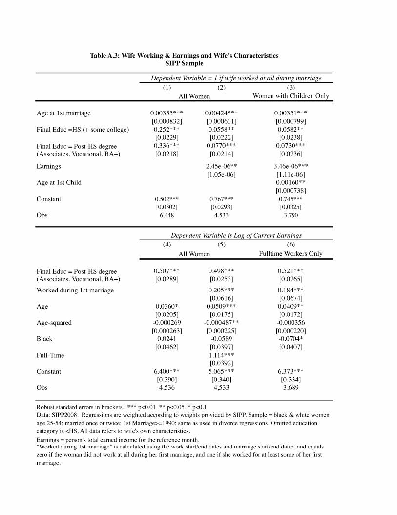
(1) (2) (3)Women with Children Only

Age at 1st marriage 0.00355*** 0.00424*** 0.00351***[0.000832] [0.000631] [0.000799]

Final Educ =HS (+ some college) 0.252*** 0.0558** 0.0582**[0.0229] [0.0222] [0.0238]0.336*** 0.0770*** 0.0730***[0.0218] [0.0214] [0.0236]

Earnings 2.45e-06** 3.46e-06***[1.05e-06] [1.11e-06]

Age at 1st Child 0.00160**[0.000738]

Constant 0.502*** 0.767*** 0.745***[0.0302] [0.0293] [0.0325]

Obs 6,448 4,533 3,790

(4) (5) (6)Fulltime Workers Only

0.507*** 0.498*** 0.521***[0.0289] [0.0253] [0.0265]

Worked during 1st marriage 0.205*** 0.184***[0.0616] [0.0674]

Age 0.0360* 0.0509*** 0.0409**[0.0205] [0.0175] [0.0172]

Age-squared -0.000269 -0.000487** -0.000356[0.000263] [0.000225] [0.000220]

Black 0.0241 -0.0589 -0.0704*[0.0462] [0.0397] [0.0407]

Full-Time 1.114***[0.0392]

Constant 6.400*** 5.065*** 6.373***[0.390] [0.340] [0.334]

Obs 4,536 4,533 3,689

Table A.3: Wife Working & Earnings and Wife's CharacteristicsSIPP Sample

Final Educ = Post-HS degree (Associates, Vocational, BA+)

Final Educ = Post-HS degree (Associates, Vocational, BA+)

Robust standard errors in brackets. *** p<0.01, ** p<0.05, * p<0.1Data: SIPP2008. Regressions are weighted according to weights provided by SIPP. Sample = black & white women age 25-54; married once or twice; 1st Marriage>=1990; same as used in divorce regressions. Omitted education category is <HS. All data refers to wife's own characteristics.Earnings = person's total earned income for the reference month."Worked during 1st marriage" is calculated using the work start/end dates and marriage start/end dates, and equals zero if the woman did not work at all during her first marriage, and one if she worked for at least some of her first marriage.

Dependent Variable = 1 if wife worked at all during marriage

Dependent Variable is Log of Current Earnings

All Women

All Women

Variables Mean Std. Dev. Obs.

Marriage intact at end of survey 0.76 0.43 827Divorced at end of survey 0.25 0.43 827Wife's age in 1980 33.87 9.15 826Husband's age in 1980 35.84 9.27 826Wife's race = white 0.89 0.32 827Wife's race = non-white 0.06 0.24 827Husband's race = white 0.89 0.32 827Husband's race = non-white 0.07 0.25 827Wife's education >HS in 1980 0.46 0.50 827Wife's education changes since 1980 0.11 0.31 827Husband's education >HS in 1980 0.55 0.50 827Husband's education changed since 1980 0.08 0.27 827Wife's religion = Protestant 0.58 0.50 827Wife's religion = Catholic 0.30 0.46 827Husband's religion = Protestant 0.55 0.50 827Husband's religion = Catholic 0.27 0.44 827Years married 28.10 11.12 827Avg # of children <18 living in HH during marriage 1.12 0.90 827Wife's age at marriage 20.39 2.77 827Husband's age at marriage 22.35 3.25 827Husband's avg % of time worked full-time during marriage 0.85 0.22 827Avg real family income 32,534.9 11,560.6 816Wife in school in 1980 0.03 0.16 826Wife worked before marriage 0.75 0.44 827*Wife's % of time worked 0.79 0.29 827High Attachment = Wife worked >75% of the time 0.68 0.47 827Wife's avg % contribution to family income 22.49 17.55 813**Wife is a "Career Woman" 0.64 0.48 697Marital Instability Index 0.32 0.33 810Marital Problems Index 2.68 2.21 797Marital Happiness Index 27.82 3.69 789Spousal Disagreement Index 3.97 1.97 738Either spouse ever talked about marital problems with others 0.64 0.48 827Either spouse ever thought marriage was in trouble 0.77 0.42 827Either spouse ever suggested divorce 0.23 0.42 827Wife was the survey respondent 0.51 0.50 827

Marital/Spousal Index values are calculated as the average value over the course of the marriage, through 1997. Marital Instability Index: Range = 0 - 1.4; higher score = more unstable. Marital Instability Index: Range = 0 - 1.4; higher score = more unstable. Spousal Disagreement Index: Range = 0-12; higher score = greater disagreement. Marital Problems Index: Range = 0-13; higher score = more marital problems.

Table A.4: Summary Statistics, MILC Sample

Sample as used in baseline regressions - includes couples where wife was at least age 18 in 1980, whose marriage did not end in widowhood. Variables are updated through 1997.* % of time worked:includes work after marriage, and during/between surveys, through 1997 (calculated during marriage only)** Career Woman: when asked, in 1997, why the wife worked, respondent said that either 'career', 'for a sense of accomplishment', 'for contact with other people', or 'for financial independence' were pretty or very important reasons.

Source: MILC (Marital Instability Over the Life Course Survey). Weighted using weights provided by MILC.

(1) (2) (3) (4)

Only wives with children

Only husbands with children

Age at marriage -0.0101 -0.00615 -0.00579 -0.000709[0.00642] [0.00848] [0.00580] [0.00841]

Educ = HS in 1980 0.0922 0.0802 0.0101 0.0313[0.0825] [0.0840] [0.0946] [0.0999]

Educ > HS in 1980 0.149* 0.152* 0.100 0.155[0.0870] [0.0896] [0.0920] [0.0967]

Education changed since 1980 0.105** 0.0937* 0.0279 0.0300[0.0483] [0.0506] [0.0667] [0.0651]

Log average real income during marriage 0.167*** 0.161*** 0.0123[0.0161] [0.0168] [0.0439]

Wife's mom worked half the time -0.0377 -0.0599 0.109***[0.0349] [0.0371] [0.0385]

Age at 1st child -0.00408 -0.00869[0.00517] [0.00562]

Constant -0.598*** -0.509** 0.595 0.821***[0.183] [0.198] [0.457] [0.167]

Observations 730 658 791 743R-squared 0.217 0.214 0.022 0.021


Omitted education category: <HS in 1980.

Table A.5 Wife's labor force attachment and Characteristics of Wife and Husband Evidence from the survey of Marital Instability over the Life Cycle

Source: MILC (Marital Instability Over the Life Course Survey). Sample includes relationships where wife was age 18+ in 1980; marriage didn't end in widowhood; without missing information; race knownDependent variable is wife's labor force attachment; attachment is calculated using wife's work start/end dates during the marriage. Attachment is low if the wife worked during 0%-75% of the marriage, and high if she worked 76% or more.Avg real income is calculated through 1997, during marriage only. Age at first child is inferred from information on other people living in HH in each survey year; survey provides age & relation to respondent of each resident.

Wife's characteristics Husband's characteristics

Dependent variable is Wife's labor force attachment

(1) (2)

Lagged Wife Work Status 0.0263 0.0234[0.0253] [0.0276]

Years married -0.0150*** -0.0193***[0.00152] [0.00209]

Wife's age at marriage -0.0129* -0.0086[0.00675] [0.00719]

Husband's age at marriage -0.0048 -0.00779[0.00522] [0.00541]

Wife >HS in 1980 0.00254[0.0319]

Husband >HS in 1980 -0.0657*[0.0344]

-0.0653***[0.0203]

Wife worked before marriage -0.0301[0.0333]

Log avg real family income 0.0355[0.0311]

Avg wife's % contrib to family income 0.000116[0.000947]

Constant 0.949*** 0.900***[0.136] [0.341]

Observations 731 712R-squared 0.185 0.221

Lagged work status is an indicator variable that equals 1 if the wife worked in the survey period prior to divorce, and 0 if she did not (it is missing if there was no information). For couples that were still married in the last survey period, the wife's work status in the previous period was used.

Table A.6: Wife's lagged work status and divorce:Evidence from the survey of Marital Instability over the Life Cycle

*** p<0.01, ** p<0.05, * p<0.1 Robust standard errors in brackets. Weighted with weights provided by MILC.Source: MILC (Marital Instability Over the Life Course Survey). Sample includes relationships where wife was age 18+ in 1980; marriage didn't end in widowhood; without missing information; race known.All regressions include controls for: Husband's and wife's race, percentage of marriage time the husband worked FT, whether acquired education after 1980 (both husband and wife), religion dummies (omitted category Protestant). Omitted categories: Low Attachment; White; <HS.Dependent variable is marital status as of the end of the interview period. Labor force, income, and number of children in HH are averages during the marriage, through 1997.



0.5

1de

nsity

0 .5 1 1.5 2 2.5Coefficient of Variation

High Attachment Low AttachmentUses regression sample as of 1997.

Figure A.1: Distribution of Coefficient of Variation ofWife’s Contribution to HH Income During Marriage

®

0.2

.4.6

.81

dens

ity

0 .5 1 1.5 2 2.5Coefficient of Variation

Career Woman Non Career WomanUses regression sample as of 1997.

Figure A.2: Distribution of Coefficient of Variation ofWife’s Contribution to HH Income During Marriage

®

Career Women and the Durability of Marriage

Documents

Transcript of Career Women and the Durability of Marriage