Cardinal Welfarism

Welfarism

■ Welfarist postulate: distribution of individual welfare across agents is only legitimate yardstick to compare states of the world

■ In cardinal version individual welfare measured by an index of utility and comparisons of utilities between individuals is meaningful

Welfarism

■ The most basic concept of welfarism is efficiency-fitness (Pareto optimality)

■ State y is Pareto superior to x if the move from x to y is by unanimous consent.

■ A state x is Pareto optimal (efficient) if there is no feasible state y Pareto superior to x

■ The task of cardinal welfarism is to pick among the feasible utility profiles one of the Pareto optimal ones.

Welfarism

■ The task of the welfarist benevolent dictator is to compare normatively any two utility profiles [(ui),(ui’)] and decide which one is best.

■ Key idea is that the comparison should follow the rationality principles of individual decision-making: completeness and transitivity

Welfarism

■ The preference relation is called a social welfare ordering, and the definition and comparison of various swo’s is the object of cardinal welfarism

■ The two most prominent instances of swo’s are the classical utilitarian and the egalitarian one.

WelfarismClassical utilitarian

Egalitarian

The classical utilitarian expresses the sum fitness principle and the egalitarian expresses the compensation principles

Welfarism

■ We will focus on “micro” versions of welfarism, e.g., problem of locating a facility where utility measures distance from facility

■ The context dictates the interpretation of utility, and in turn, influences the choice of the swo

■ The ability to objectively measure and compare utilities can be more or less convincing (distance, vitamins vs. pleasure from eating cake, or observing art)

Welfarism

■ Microwelfarist viewpoint separates the allocation problem at stake from the rest of our agent’s characteristics

Assumes my utility level measured independently of unconcerned agents Separapility property is the basis of the additive representation

■ From this axiomatic analysis three paramount swo’s emerge: classical utilitarianism, egalitarianism, Nash collective utility function

Additive Collective Utility Function

■ Two basic requirements of swo. ■ Monotonicity:

Additive Collective Utility Functions

■ Most swo’s of importance are represented by a collective utility function, namely a real-valued function W(u1,…un) with the utility profile for argument and the level of collective utility for value.

Additive Collective Utility Functions

■ A key property of welfarist rationality is independence of unconcerned agents. It means that an agent who has no vested interest in the choice between u and u’ because his utility is the same in both profiles, can be ignored.

Additive Collective Utility Functions

■ Theorem: the SWO is continuous and IUAs iff it is represented by an additive CUF, where g is an increasing and continuous function.

( ) ( )iiW u g u=∑

Additive Collective Utility Functions

■ The Pigou-Dalton transfer principle (fairness property) expresses an aversion for “pure” inequality

■ Say that u1<u2 at profile u and consider a transfer of utility from 2 to 1 where u1’ ,u2’ are the utilities after the transfer st:

■ u1< u1’ ,u2’ <u2 and u1’ +u2’ =u1+u2 ■ The P-D transfer principle requires that swo

increases in a move reducing inequality between agents {for additive g(u1)+g(u2) ≤ g(u1’ )+g(u2’ ) which is equivalent to concavity of g}

Additive Collective Utility Functions

■ An invariance property: independence of common scale (ICS) requires us to restrict attention to positive utilities, and states that a simultaneous rescaling of every individual utility function does not affect the underlying swo.

Additive Collective Utility Functions

■ For an additive cuf the ICS property holds true for a very specific family of power functions.

g(z)=zp for a positive p g(z)=log(z) g(z) = -z-q for a positive q

Additive Collective Utility Functions

■ The corresponding cuf W take the form

Comparing Classical Utilitarianism, Nash, and Leximin■ The central tension between classical utilitarian

and egalitarian welfarist objectives is that in the former the welfare of a single agent may be sacrificed for the sake of improving total welfare (the slavery of the talented) while in the latter large amounts of joint welfare may be forfeited in order to improve the lot of the worst of individual

■ Examples follow:

Egalitarianism and the Leximin Social Welfare Ordering■ We focus on the welfarist formulation of the compensation

principle as the equalization of individual utilities ■ Example 3.1 Pure Lifeboat Problem suppose five agents

labelled {1,2,3,4,5} and feasible subsets (less dramatic software program, background music with 6 programs to choose from):

■ {1,2} {1,3} {1,4} {2,3,5} {3,4,5} {2,4,5}All outcomes Pareto optimalSuppose utility of staying on boat is 10, swimming 1

■ Utilitarian and egalitarian arbitrator make same choice ■ Subsets of 3 equally good but better than subsets of 2 utilitarian

30>20, lexicographic (1,1,10,10,10) preferred to (1,1,1,10,10)

19

Agent 1 2 3 4 5Utility g 10 6 6 5 3Utility b 0 1 1 1 0

Now assume individual utilities vary across individuals, e.g., tastes for radio programs

■ {1,2}=18, {1,3}=18, {1,4} =16, {2,3,5}=16, {3,4,5}=15, {2,4,5}=15

⇒ {1,2} ∼ {1,3} ≻ {1,4} ≻ {2,3,5} ≻ {3,4,5} ∼ {2,4,5}

Utilitarian calculus:

Example 3.1 Pure Lifeboat Problem (different utilities)

(note numbers different from text)

20

Example 3.1 Pure Lifeboat Problem (different utilities)

The egalitarian arbitrator, by contrast, prefers any three-person subset over any two person one; his ranking follows:

Agent 1 2 3 4 5Utility g 10 6 6 5 3Utility b 0 1 1 1 0

Leximin swo

■ Also called egalitarian swo and sometimes “practical egalitarianism”

■ Given two feasible utility profiles u and u’ we arrange them first in increasing order, from the lowest to highest utility, and denote the new profiles u* and u’*:

* * * '* '* '*1 2 1 2... ...n nu u u and u u u≤ ≤ ≤ ≤ ≤ ≤

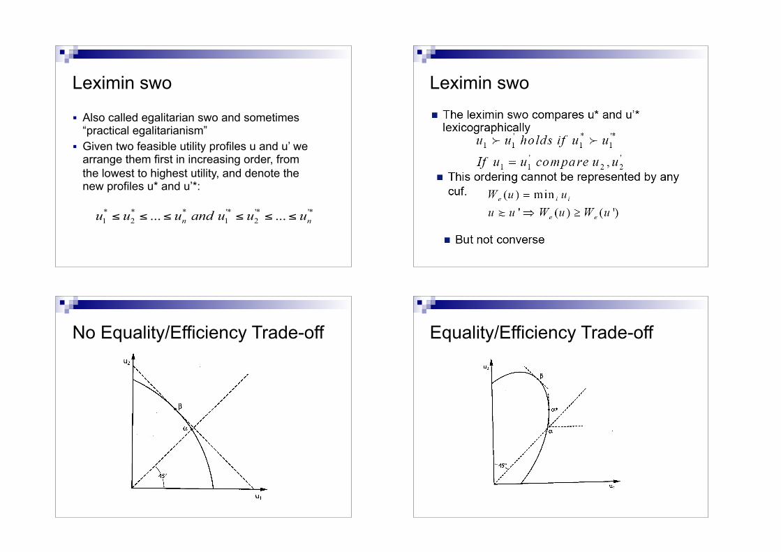
Leximin swo

Νο Equality/Efficiency Trade-off Equality/Efficiency Trade-off

No equality/efficiency trade-off Equality/efficiency trade-off

Leximin

■ The leximin ordering is preserved under a common arbitrary (nonlinear) rescaling of the utilities. Thus the comparison of u versus u’ is the same as that of v=(u)2 versus v’=(u’)2, or of (eui+Sqrt[ui]) verus (eui’+Sqrt[ui’]), etc.

■ This property is called independence of the common utility pace

■ Leximin is not the only swo icup, but it is the only one that also respects the Pigou-Dalton transfer principle.

Example: Location of a facility

■ A desirable facility must be located somewhere in the interval [0,1], representing a “linear” city

■ Each agent lives at a specific location xi in [0,1]; if the facility is located at y, agent I’s disutility is the distance |y-xi|.

■ The agents are spread arbitrarily along interval [0,1] and the problem is to find a fair compromise location

Example: Location of a facility

■ The unique egalitarian optimum is the midpoint of the range of our agents.

■ Classical utilitarianism chooses the median of the distribution of agents, namely the point yu st at most half of the agents live strictly to the left of yu and at most half of them strictly to the right

■ The interpretation of the facility has much to do with the choice between the two solutions

Information booth, swimming pool =>clas. util Post office, police station (basic needs)=>egal

Example: Location of a facility

■ The Nash collective utility function is not easy to use in this example because the natural zero of individual utilities is when the facility is located precisely where the agent in question lives, say xi: then we set ui(y)=-|y-xi| if the facility is located at y.

■ The Nash utility is not defined when some utilities are negative; therefore we must adjust the zero of each agent.

■ The choice of one or another normalization will affect the optimal location for the Nash collective utility.

Example: Location of a facility

■ The great advantage of the classical utilitarian utility is to be independent of individual zeros of utilities

■ If we replace utility ui=-|y-xi| by u1i or u2i for any number of agents, the optimal utilitarian location remains the median of the distribution and the preference ranking between any two locations does not change

■ This independence property uniquely characterizes the classical utilitarian among all cufs.

u1i (y) = 1− y − xiu2i (y) = xi − y − xi if xi ≥1/ 2

u2 j (y) = 1− x j − y − x j if x j ≤1/ 2

Example 3.6a Time-Sharing

■ n agents work in a common space (gym) where the radio must be turned on one of five available stations

■ As their tastes differ greatly they ask the manager to share the time fairly between the five stations

■ Each agent likes some stations and dislikes some; if we set her utility at 0 or 1 for a station she dislikes or likes we have a pure lifeboat problem

■ The difference is that we allow mixing of timeshares xk (k=1,...,5) st x1+…+x5=1

33

Example 3.6a Time-Sharing■ Classical utilitarian chooses “tyranny of the

majority”: station with largest support played all the time

■ Egalitarian manager exactly opposite: pays no attention to size of support and plays each station 1/5th of the time (provided each station has at least one fan)

■ Nash collective utility picks an appealing compromise between the two extremist solutions:

34

Example 3.6a Time-Sharing■ The relative size of nk matter and everyone

is guaranteed some share of her favourite station

maxxk

L = nk ln xk + λ(1− xx )∑∑⇒ xk =

nkn

Example 3.6b Time-Sharing

A B C D E1 1 0 0 0 02 0 1 0 0 03 0 0 1 1 04 0 0 0 1 15 0 0 1 0 1

Five agents share a radio and the preferences of 3 of them are somewhat flexible in the sense that they like two of the five stations according to the following pattern

36

Example 3.6b Time-Sharing■ Utilitarian manager shares the time

between the three stations c, d, and e but never plays stations a and b

A B C D E1 1 0 0 0 02 0 1 0 0 03 0 0 1 1 04 0 0 0 1 15 0 0 1 0 1

37

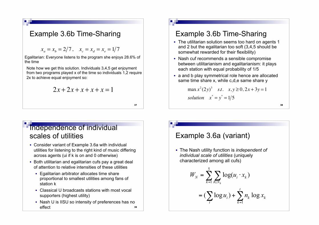
Example 3.6b Time-Sharing

xa = xb = 2 7, xc = xd = xe = 1 7

2x + 2x + x + x + x = 1

Note how we get this solution. Individuals 3,4,5 get enjoyment from two programs played x of the time so individuals 1,2 require 2x to achieve equal enjoyment so:

Egalitarian: Everyone listens to the program she enjoys 28.6% of the time

38

Example 3.6b Time-Sharing■ The utilitarian solution seems too hard on agents 1

and 2 but the egalitarian too soft (3,4,5 should be somewhat rewarded for their flexibility)

■ Nash cuf recommends a sensible compromise between utilitarianism and egalitarianism: it plays each station with equal probability of 1/5

■ a and b play symmetrical role hence are allocated same time share x, while c,d,e same share y

max x2 (2y)3 s.t. x, y ≥ 0, 2x + 3y = 1solution x* = y* = 1 5

39

Independence of individual scales of utilities■ Consider variant of Example 3.6a with individual

utilities for listening to the right kind of music differing across agents (ui if k is on and 0 otherwise)

■ Both utilitarian and egalitarian cufs pay a great deal of attention to relative intensities of these utilities ■ Egalitarian arbitrator allocates time share

proportional to smallest utilities among fans of station k

■ Classical U broadcasts stations with most vocal supporters (highest utility)

■ Nash U is IISU so intensity of preferences has no effect

Example 3.6a (variant)

■ The Nash utility function is independent of individual scale of utilities (uniquely characterized among all cufs)

5

1

1

log( )

( log ) log

k

N i kk i N

t

i k ki k

W u x

u n x

= ∈

=

= ⋅

= +

∑∑

∑ ∑

Bargaining Compromise■ Bargaining compromise places bounds on individual utilities

that depend on physical outcomes of the allocation problem (thus moves a step away form strict welfarism)

■ The choice of the zero and/or the scale of individual utilities is crucial whenever a swo picks the solution (exception is clas u. that is ind of zeros, Nash ind of utility scales)

■ The bargaining version of welfarism incorporates an objective definition of the zero of individual utilities (which corresponds to the worst outcome from the point of view of the agent).

■ The bargaining approach then applies the scale invariant solution to the zero normalized problem, which in turn ensures that the solution is independent of both individual zeros and scales of utilities (Nash and Kalai-Smorodinsky two prominent methods)

Example 3.11

A B CAnn 60 50 30Bob 80 110 150

■ Two companies (Ann, Bob) selling related yet different products and share retail outlet

■ Can set up outlet in three different modes denoted a,b,c that bring following volumes of sales (000s $)

Example 3.11

A B CAnn 60 50 30Bob 80 110 150

■ Only interested in maximising volume of sales (not same as profits) and transfers not allowed

■ Only tool for compromise is time-sharing among three modes: over years season they can mix them in arbitrary proportions st x+y+z=1

Example 3.11

A B CAnn 60 50 30Bob 80 110 150

■ Applying welfarist solutions to raw utilities makes little sense, e.g., egalitarian would pick outcome where Ann’s u is highest but the fact that her business yields smaller volumes of sales should not matter

■ Issue is to find a compromise between three feasible outcomes over which agents have oposite preferences

Example 3.11

A B CAnn 30 20 0Bob 0 30 70

■ Total u in class util is similarly irrelevant ■ Need to find a fair compromise that

depends neither on scale nor on the zero of both individuals

■ For minimal u of either player we pick the lowest feasible volume of sales: 30K for Ann and 80K for Bob. This yields…

Example 3.11

A B CAnn 30 20 0Bob 0 30 70Time shares x y z

■ The idea of random ordering suggests letting Ann and Bob each have their way 50% of the time x=z=1/2 that would lead to a normalized utility vector of (15,35)

■ However, y’=0.8, z’=2 yields (16,38) hence Pareto superior

47

Example 3.11

max log(30 20 ) log(30 70 )1, , , 0

30 20 30 70max

30 701, , , 0

x y y zunder x y z x y z

x y y z

under x y z x y z

+ + +

+ + = ≥

+ +=

+ + = ≥

Nash Eq. (8)

Kalai-Smorodinksy Eq. (9)

The KS solution equalizes the relative gains (fraction of maximal feasible gains) of all agents

49

Example 3.11

maxln(20y)+ ln(30y + 70(1− y))= maxln(20)+ log y + ln(70 − 40y))∂∂y: 1y− 4070 − 40y

= 0⇒ 40y = 70 − 40y⇒ y = 7 / 8

Nash solution:

In this case since the feasibility set is a kinked line we know it will be either on segment CB or segment BA. Need to check where highest utility achieved. In this case it turns out to be on segment CB (x=0 and z=1-y)

50

Example 3.11 K-S solution:

max 30x + 20y30

= 30y + 70z70

st x + y + z = 1

AB : z = 0⇒ y = 1− x10x + 2030

= 30 − 30x70

⇒ x = − 516

Can’t have negative so KS must lie on BC

BC : x = 0⇒ z = 1− y20y30

= 70 − 40y70

⇒ y = 2126

Example 3.11

■ Nash sol: y=7/8, z=1/8 => u1=17.5, u2=35 ■ KS sol: y=21/26, z=5/26=>u1=16.1,u2=37.7

■ Note that both solutions are superior to the random dictator outcome a/2+c/2 (with associated utilities 15,35). This is a general property of our two bargaining solutions.