CARDIAC SIGNAL PROCESSING FOR CLASSIFICATION OF ...

1

CARDIAC SIGNAL PROCESSING FOR CLASSIFICATION OF

SUPRAVENTRICULAR TACHYCARDIA USING INTRACARDIAC SIGNALS

By

NAUMAN RAZZAQ

A DISSERTATION

Submitted to

National University of Sciences and Technology

in partial fulfillment of the requirements for the degree of

DOCTOR OF PHILOSOPHY

Supervised by

DR SYED MUHAMMAD TAHIR ZAIDI

College of Electrical and Mechanical Engineering

National University of Sciences and Technology, Pakistan

2017

2

In the name of Allah, the most Merciful and the most Beneficent

3

ABSTRACT

CARDIAC SIGNAL PROCESSING FOR CLASSIFICATION OF

SUPRAVENTRICULAR TACHYCARDIA USING INTRACARDIAC SIGNALS

By

NAUMAN RAZZAQ

Electrophysiology study (EPS), a minimal invasive procedure, is performed in Cath

lab for investigation and therapeutic treatment of abnormality in cardiac rhythm using

Intracardiac Electrogram (IEGM) and Electrocardiogram (ECG) signals. IEGM signals

are acquired via catheters placed inside heart, and ECG signals are collected using

surface catheters. The complex patterns of IEGM signals are studied with different

protocols for identification of cardiac abnormalities. Study is carried out visually by

Electro physiologists using the monitor screens to determine key features and their

intervals, which is time consuming and highly dependent on individual expertise.

In this work, IEGM signals have been used to design an automated Supraventricular

Tachycardia (SVT) differentiation system during EPS. The system will assist the

electrophysiologist by reducing the manual working and time involved in diagnosis of

SVT arrhythmia. The research has been conducted in three phases. In Phase I,

preprocessing of the IEGMs have been undertaken for removal of power line interference

and electromyographic noises. In Phase II, classification of Atrioventricular Node

4

Reentrant Tachycardia and Atrioventricular Reentrant Tachycardia have been carried out

in time domain. In Phase III, non-parametric spectral estimation of IEGM signals have

been used for differentiation between Normal Sinus Rhythm, Atrial Tachycardia, Atrial

Flutter and Atrial Fibrillation.

5

To

Islamic Republic of Pakistan

6

ACKNOWLEDGEMENTS

I praise Almighty Allah Subhanahu wa Ta’ala for all his mercy and grace, the strength

that he gave me strength to accomplish this research and complete my PhD.

I would like to express my sincerest gratefulness for the guidance and support of all

my teachers whose intense efforts have made possible the efficacious completion of this

work. The knowledge that I obtained from them proved advantageous throughout the

path of my studies. I would like to express gratitude to my supervisor, Dr Syed

Muhammad Tahir Zaidi, both for accommodating me as his PhD student and for

imparting beneficial guidance, counseling and support over the years leading towards the

completion of this thesis. I would like to express my sincere gratitude to my GEC

members Dr Qaiser Chaudhry, Dr Hamid Mehmood Kamboh, Dr Imran Akhtar for their

precious time and guidance that I have received from them. I would address special

thanks to Dr Muhammad Salman who as a senior always selflessly helped and supported

me in my research work. I would like to convey my earnest appreciation to Col Nasir

Rasheed, Dr Umer Shabaz, Dr. Nauman Anwar, Dr Muhammad Khurram and Dr Atif

Ali, for their valuable time, consideration and encouragement. I gratefully acknowledge

the assistance I received from Lt Col Shafaat al Sheikh, Lt Col Rahat Ali, Dr Khalid

Munawar, Maj Dr Nauman and all colleagues with me in EME College.

I am obligated to my wife and children who have been very compliant / supportive and

have shown remarkable patience all the way along. I am also obliged to my family elders

7

and my sister who have been sources of encouragement for me and their prayers have

complemented me throughout my life.

I would also like to thankfully acknowledge National University of

Sciences and Technology (NUST) for the financial assistance they provided for my

studies and research.

8

TABLE OF CONTENTS

Abstract .................................................................................................................. 3

Acknowledgements ............................................................................................................. 6

Table of contents ................................................................................................................. 8

List of figures ................................................................................................................ 11

CHAPTER 1 INTRODUCTION

1.1 Choosing the Research in Intracardiac Signals ...................................................20

1.2 Problem Statement ........................................................................................22

1.3 Research Approach ........................................................................................22

1.4 Thesis layout ........................................................................................23

CHAPTER 2 CARDIAC ELECTROPHYSIOLOGY

2.1 Anatomy of Heart ........................................................................................27

2.2 Cardiac Conduction System ................................................................................28

2.3 Normal Sinus Rhythm ........................................................................................37

2.4 Arrhythmia ........................................................................................38

2.5 The Origins of Arrhythmia .................................................................................40

2.6 Supraventricular Tachycardia .............................................................................46

CHAPTER 3 ACQUISITION OF CARDIAC ELECTRIC SIGNALS

3.1 Electrocardiogram ........................................................................................53

3.2 The Intracardiac Electrogram .............................................................................62

3.3 Cardiac Catheterization for EP Study .................................................................64

9

CHAPTER 4 PRE-PROCESSING OF INTRACARDIAC SIGNALS

4.1 Scope of Pre-Processing .....................................................................................73

4.2 Power Line Interference ......................................................................................76

4.3 Base Line Wander ......................................................................................114

4.4 Electromyographic Noise ..................................................................................115

CHAPTER 5 TEMPORAL FEATURES OF INTRACARDIAC SIGNALS

5.1 Literature Review ......................................................................................122

5.2 Data Collection ......................................................................................123

5.3 Methodology ......................................................................................125

5.4 Feature Detection ......................................................................................135

5.5 Results ......................................................................................143

5.6 Summary ......................................................................................143

CHAPTER 6 IDENTIFICATION OF REENTRANT TACHYCARDIA


6.2 Dataset ......................................................................................145

6.3 Methodology ......................................................................................146

6.4 Identification of AVNRT ..................................................................................150

6.5 Identification of AVRT .....................................................................................154

6.6 Classification Algorithm between AVRT and AVNRT ...................................156

6.7 Summary ......................................................................................159

CHAPTER 7 FREQUENCY ANALYSIS FOR IDENTIFICATION OF AT


7.2 Dataset ......................................................................................163

10

7.3 Methodology ......................................................................................165

7.4 IEGM Pre- Processing ......................................................................................167

7.5 PSD Estimation ......................................................................................167

7.6 Extraction of Spectral Parameters from PSD....................................................169

7.7 Algorithm for Discrimination of Atrial Arrhythmias .......................................175

7.8 Results and Discussion .....................................................................................176

7.9 Accuracy Analysis .....................................................................................182

7.10 Summary ......................................................................................184

Conclusion and future Work

Conclusion ......................................................................................185

Future Recommendations ......................................................................................186

Acknowledgement ......................................................................................188

11

LIST OF FIGURES

Figure 1-1 Research approach and outcomes .......................................................... 24

Figure 2-1 The valves and chambers inside heart ................................................... 28

Figure 2-2 Cells of Electric Conduction System of Heart ....................................... 29

Figure 2-3 Phases of a cardiac AP. ......................................................................... 31

Figure 2-4 Phases of a AP of cardiac pacemaker cells. .......................................... 32

Figure 2-5 The AP patterns of various cardiac cells ............................................... 33

Figure 2-6 Depolarization –polarization cycle of Pacemaker Cell ......................... 33

Figure 2-7 Intrinsic Conduction system of the heart ............................................... 34

Figure 2-8 The sequence of electric excitation ........................................................ 36

Figure 2-9 Extrinsic conduction system controlled by ANS ................................... 38

Figure 2-10 Ventricular ectopic foci.......................................................................... 41

Figure 2-11 Right sided, septal and left sided APs ................................................... 42

Figure 2-12 Local and global reentry ........................................................................ 43

Figure 2-13 Normal versus reentry mechanism......................................................... 43

Figure 2-14 (a) AVNRT case, (b) AVRT case .......................................................... 45

Figure 2-15 Normal cardiac cycle versus pre-excited cycle ...................................... 46

Figure 2-16 Normal atrial activation versus Atrial Fibrillation ................................. 48

Figure 2-17 Normal cardiac conduction and AVNRT case....................................... 50

Figure 2-18 Orthodromic AVRT .............................................................................. 51

Figure 3-1 Accumulative effect of AP of various cardiac conduction cells ............ 54

Figure 3-2 Complete rhythm of depolarization/repolarization ................................ 55

12

Figure 3-3 The waveform/segment description of an ECG signal .......................... 56

Figure 3-4 Scheme of 10 electrodes placement (12 leads ECG) ............................. 57

Figure 3-5 The combination of limb leads .............................................................. 58

Figure 3-6 The combination of augmented limb leads ............................................ 59

Figure 3-7 The view angles in vertical plane .......................................................... 59

Figure 3-8 The view angles by six precordial leads in horizontal plane ................. 61

Figure 3-9 The complete three dimensional view by 12 leads ECG ....................... 61

Figure 3-10 Catheter placement procedure................................................................ 63

Figure 3-11 EP catheter electrode.............................................................................. 64

Figure 3-12 Bi-polar catheter configuration .............................................................. 65

Figure 3-13 Basic configuration of HRA, His, RVA and CS catheters .................... 66

Figure 3-14 Correlation between IEGM and ECG features ...................................... 67

Figure 3-15 Layout of EP study layout containing ECG and IEGM leads ............... 68

Figure 3-16 Propagation of ‘A’ wave sequentially from RA to CS leads ................. 69

Figure 3-17 Appearance of ‘A’-wave and ‘V’-wave ................................................. 70

Figure 3-18 Antegrade Versus Retrograde Pacing .................................................... 71

Figure 4-1 Stages of Arrhythmia Classification Algorithm ..................................... 73

Figure 4-2 Effect of inappropriate frequency band selection. ................................. 75

Figure 4-3 Effects of a notch filter for removal of PLI........................................... 75

Figure 4-4 IEGM data sampled at 2 kHz ................................................................. 80

Figure 4-5 Frequency spectrum of Raw IEGM signal............................................. 81

Figure 4-6 Proposed layout for elimination of PLI and its harmonics .................... 84

Figure 4-7 Intelligent DFT - Flow chart. ................................................................. 87

13

Figure 4-8 Working of intelligent DFT. .................................................................. 88

Figure 4-9 (a) Non-overlapping window (b) Half window overlapping ................. 91

Figure 4-10 Sliding window DFT and delay caused. ................................................ 92

Figure 4-11 Working of SSRLS. ............................................................................... 95

Figure 4-12. IEGM Test signal with sampling rate of 2000 samples/sec. ................. 96

Figure 4-13 Frequency spectrum of IEGM Test signal ............................................ 97

Figure 4-14 The composite test signal ....................................................................... 98

Figure 4-15 PLI corrupted IEGM signal ................................................................... 99

Figure 4-16 Frequency spectrum of PLI corrupted IEGM signal.............................. 99

Figure 4-17 PLI frequency estimation in stages ...................................................... 100

Figure 4-18 Frequency estimation through proposed scheme.. ............................... 101

Figure 4-19 Tracking of SSRLS adaptive filter during initialization period .......... 103

Figure 4-20 Filtered IEGM signal after initialization .............................................. 103

Figure 4-21 Frequency spectrum of tracked/filtered signals.. ................................. 104

Figure 4-22 Raw IEGM signal corrupted with PLI. ................................................ 105

Figure 4-23 Frequency spectrum of raw IEGM signal. ........................................... 105

Figure 4-24 Frequency spectrum of filtered IEGM. ................................................ 106

Figure 4-25 Filtration quality of SSRLS adaptive filter and notch filter. ............... 108

Figure 4-26 The filtered output with step change in PLI......................................... 109

Figure 4-27 The filtered outputs with ramp change in PLI. .................................... 110

Figure 4-28 Comparison of proposed system and notch filter with ramp change. .. 111

Figure 4-29 Frequency estimation by intelligent DFT ............................................ 112

Figure 4-30 Comparison of proposed system & notch filter with frequency shift. . 113

14

Figure 4-31 Filtered IEGM signal from proposed method. ..................................... 117

Figure 4-32 Preservation of ‘H’ feature with SG filter............................................ 118

Figure 4-33 EMG removal from IEGM through MA filter ..................................... 119

Figure 4-34 EMG removal from IEGM through IIR Filter ..................................... 120

Figure 4-35 EMG removal from IEGM through Median Filter .............................. 121

Figure 5-1 AFIC dataset containing 3xECGs and 9xIEGMs ................................ 124

Figure 5-2 MIT dataset containing 3xECGs and 5xIEGMs .................................. 125

Figure 5-3 Catheters arrangement for SVT arrhythmia detection ......................... 126

Figure 5-4 Proposed system for feature detection ................................................. 127

Figure 5-5 Straight Pacing. .................................................................................... 128

Figure 5-6 Extra Stimuli Pacing. ........................................................................... 129

Figure 5-7 Algorithm for detection of PES protocol ............................................. 131

Figure 5-8 HisP with pacing artifact ...................................................................... 132

Figure 5-9 HisP with pacing artifact removed. ...................................................... 133

Figure 5-10 IEGM of His catheter without envelop ................................................ 134

Figure 5-11 IEGM of His catheter after applying envelop detect ........................... 134

Figure 5-12 IEGM signals of His distal and proximal ............................................ 135

Figure 5-13 Onset of VRVA ...................................................................................... 136

Figure 5-14 Onset of AHRA ...................................................................................... 137

Figure 5-15 Earmarking of VHis-on and VHis-off ......................................................... 139

Figure 5-16 Marking of HHis-on on His IEGM......................................................... 140

Figure 5-17 Feature detection algorithm ................................................................. 142

Figure 6-1 Proposed methodology for detection of AVNRT/AVRT .................... 146

15

Figure 6-2 Extra stimulus pacing at HRA. ............................................................ 147

Figure 6-3 Correlation of electric activity in different electrodes. ......................... 149

Figure 6-4 Interval measurements. ........................................................................ 150

Figure 6-5 Slow-fast AVNRT and observation during EP study. ......................... 151

Figure 6-6 Presence of AH jump with extra stimulus pacing protocol. ................ 152

Figure 6-7 AH jump............................................................................................... 153

Figure 6-8 AH Interval and AH Jump measurement ............................................. 154

Figure 6-9 (a) Orthodromic AVRT (b) Antidromic AVRT................................... 155

Figure 6-10 Reentrant arrhythmia detection algorithm ........................................... 156

Figure 7-1 Pre-processing steps HRA-IEGM ........................................................ 166

Figure 7-2 Signal segment and Sub Segment for Estimation of PSD. .................. 168

Figure 7-3 Calculation of RI for reliability of DF ................................................. 170

Figure 7-4 PSD comparison of regular and irregular arrhythmias ....................... 171

Figure 7-5 The Description of APSR. ................................................................... 173

Figure 7-6 Differentiation Algorithm based on DF and APSR. ............................ 175

Figure 7-7 NSR case: DF is at 1.46 Hz and APSR value is 0.903. ....................... 177

Figure 7-8 AT Case: DF is at 2.68 Hz and APSR value is 0.993. ........................ 178

Figure 7-9 AT Differentiation from AF (3~4 Hz). ................................................ 178

Figure 7-10 AFL Differentiation from AF (4~5 Hz). .............................................. 179

Figure 7-11 AF Differentiation from AT (3~4 Hz). ................................................ 180

Figure 7-12 AF Differentiation from AFL (4~5 Hz). .............................................. 180

Figure 7-13 AF Detection (5~12 Hz) ...................................................................... 181

16

LIST OF TABLES

Table 4-1. Filtration requirement for ECG/IEGM signals ............................................ 74

Table 4-2 FFT, DFT and intelligent DFT comparison ................................................. 89

Table 5-1 Result of Feature Detection Algorithm .................................................... 143

Table 6-1 Result of Arrhythmia Detection ............................................................... 157

Table 6-2 Sensitivity, Specificity, PPV and NPV Results ....................................... 158

Table 7-1 ECG and IEGM Data – AFIC/NIHD ....................................................... 163

Table 7-2 ECG and IEGM Data – MIT Physiobank ................................................ 164

Table 7-3 IEGM Dataset (Verified Rhythms) .......................................................... 165

Table 7-4 RI and APSR comparison ........................................................................ 175

Table 7-5 Rhythm detection results by proposed method ....................................... 182

Table 7-6 Sensitivity, Specificity, PPV and NPV Results ....................................... 183

17

LIST OF ABBREVIATIONS

AP Action Potential

APs Accessory Pathways

AVNRT Atrioventricular Node Reentrant Tachycardia

AVRT Atrioventricular Reentrant Tachycardia

AT Atrial Tachycardia

AFL Atrial Flutter

AF Atrial Fibrillation

AV Atrio Ventricular

A wave Atrial Wave

ANS Autonomic Nervous System

APSR Average Power Spectral Ratio

AFIC Armed Forces Institute of Cardiology

ANC Adaptive noise cancellation

BLW Base Line Wander

bpm beats per minute

CS Coronary Sinus catheter

DF Dominant frequency

Dst Distal

DFT Discrete Fourier Transform

EPS Electrophysiology study

ECG Electrocardiography

18

EMG Electromyographic

FIR Finite Impulse Response

HRA High Right Atrium Catheter

His His bundle catheter

H wave His Bundle wave

IEGM Intracardiac Signals

ICD Implantable Cardioverter Defibrillator

IIR Infinite Impulse Response

ISSAD Intracardiac Signal Analysis And Display

LA Left Atrium

LV Left Ventricle

LBB Left Bundle Branch

LMS Least Mean Square

NIHD National Institute of Heart Diseases

NSR Normal Sinus Rhythm

PLI Power Line Interference

Prx Proximal

PES Programmed Electrical Stimulation

PSD Power Spectral Density

RI Regularity Index

RA Right Atrium

RV Right Ventricle

RVA Right Ventricular Apex Catheter

19

RLS Recursive Least Square

RBB Right Bundle Branch

SVT Supraventricular Tachycardia

SA Sinoatrial

SG Savitzky–Golay

SVC Superior Vena Cava

SSRLS State Space Recursive Least Square

V wave Ventricular wave

VT Ventricular Tachycardia

WHO World Health Organization

20

CHAPTER 1

INTRODUCTION

1.1 Choosing the Research in Intracardiac Signals

As per survey report held by World Health Organization (WHO), major cause of human

deaths are because of heart diseases [1, 2]. In 2013, deaths because of cardiac issues,

represented 31% of global deaths affecting about 17.3 million people [2]. Keeping in

view this trend, it is expected that the cardiac related deaths may touch the figure of 23.6

million in 2030 [3, 4]. Cardiac problem can be related to cardiovascular or arrhythmia

(abnormality in rhythm). If we take into account the arrhythmia’s statistics, approx 1 in

18 (or 5.30%) are affected from arrhythmia related disorders. In US, more than 850,000

people are hospitalized for a problem related to arrhythmia each year and 100,000

American have an implantable Defibrillator (ICD) [5].

Electrocardiogram (ECG) is the recording of cardiac signals from surface of patient’s

body and commonly used to gauge heart’s rhythm related problem however, sometimes

ECG does not fulfill the purpose. As an alternate, the invasive method is adopted known

as Electrophysiology (EP) study (named as EPS), in which heart‘s electric signals are

procured directly by inserting catheter electrodes inside the heart. The signals recorded

through EPS are known as Intracardiac Electrograms (IEGM). EPS has made a noticeable

evolution in the last three decades and has emerged as a major specialty in cardiology.

EPS is comparatively complicated field and it requires in depth understanding of several

21

diagnostic procedures and pacing protocols of IEGMs. That is why a very few

cardiologists opt to specialize in this field.

I am an electrical engineer and I did several specialization courses related to biomedical

field during my services in armed forces. When I joined for PhD, I was serving in Armed

Forces Institute of Cardiology (AFIC) as Biomed Engineer and being directly involved

with the Cardiac related equipment, I developed my interest to undertake research in this

field.

In Pakistan, the EPS setups are very few. One of major issue related to EPS is the non-

standardization of EPS protocols across the world and the heart is stimulated externally at

different loci under various protocols to study its behavior.

At present, the EP study is based on manual measurements on screen by the

electrophysiologist, that is a time consuming procedure because of manual marking of

features and their interval measurement and the procedure may prolong to many hours in

some cases.. It is highly desired that automated arrhythmia detection based on IEGMs be

developed, which will facilitate the electrophysiologist.

EPS is highly demanding field and has lot of potential for research in this area. Because

of technical in nature, EP study demands the involvement of an engineer in this field who

can investigate the IEGM signals and new methods can be explored with application of

different analysis tools. Lot of work can be found in literature for automated arrhythmia

detection based on ECG, however very few or no published material is available in the

field of automated arrhythmia classification based on IEGMs. Moreover, it has been

observed that the EP study is mostly based on time domain analysis by defining temporal

22

relationship between different features of IEGMs manually. The application of frequency

domain analysis for differentiation among different arrhythmias has vast room of

exploration in EP study.

1.2 Problem Statement

SVT encompasses all arrhythmias which are above ventricular, this includes arrhythmias

related to atrium, SA node and atrioventricular (AV) node [6]. SVT is a commonly found

arrhythmia, which affects over 570,000 people each year [7]. The SVT prevalence in the

general population is 0.229% of total human population [7, 8]. The vast majority of SVTs

are one of three types; atrioventricular nodal re-entrant tachycardia (AVNRT) which is

responsible for approximately 65% of cases, atrioventricular reentrant tachycardia

(AVRT) which is responsible for approximately 30% of cases, and atrial tachycardia

(AT) responsible for approximately 5% of cases [9-11].

In this research work, I choose SVT arrhythmias for differentiation of its various types by

analyzing IEGM signals. This research work intends to develop an automated arrhythmia

differentiator based on time and frequency domain analysis, to be applied on IEGMs

acquired during clinical EPS, designed specifically to focus on Supraventricular

Tachycardia (SVT).

1.3 Research Approach

The overall research aimed to develop a project named as “Intracardiac Signal Analysis

And Display” (ISSAD) which acquire, pre-process and classify among various

arrhythmias of SVT in first phase and to classify ventricular tachycardia (VT) as future

23

target (in next phase). For this purpose a research group headed by me as PhD Scholar

and 4~5 Master students, was formulated to cover the scope of this research. The

research approach and outcomes from this research are shown in Figure 1-1. Since this

field is quite complex, therefore the involvement of electrophysiologist and acquiring

sufficient medical related knowledge was the base line to move fwd. ECG databank of

various arrhythmias can be found at MIT Physiobank, however databank of IEGM

signals is rarely found.

The acquisition of SVT arrhythmia relevant IEGM dataset was a difficult task because

the complete range of gold standard dataset was not available on Physionet or any other

authentic resource. Therefore, the majority of required Patient’s dataset was collected

from AFIC/NIHD Pakistan and few from MIT Physionet database as available [12]..

These dataset was verified from expert electrophysiologist for the specific type of

arrhythmias and then it was referred as gold standard for research work.

Overall, research was focused on SVT and it conducted undertaken sequentially in three

main fields, 1) Pre-processing of IEGMs, 2) The classification of reentrant tachycardia in

time domain & 3) The classification of atrial tachycardias in frequency domain. As the

outcome of this research, the project ISAAD was successfully developed.

1.4 Thesis layout

The overall thesis can be grouped into two parts. Part I consist of chapters 1, 2 and 3

which generally cover the motivation, database acquisition and background knowledge

related to this topic. Part II consist of chapters 4, 5, 6 and 7 which present the proposed

methods, worked out of this research work. Since this thesis dissertation covers the

diverse fields including pre-processing and classification of IEGMs in time domain and

24

frequency domains, the related literature review have not been grouped together rather it

has been covered prior to related field.

Figure 1-1 Research approach and outcomes

The background knowledge and research work undertaken has been grouped into seven

chapters. The first chapter elaborates the brief background of the selected topic along

with motivation for its selection. The research problem has been formulated and its

objectives are defined in this chapter. The resource database has also been declared.

25

In second chapter, the anatomy of heart and role of electric conduction system in cardiac

functioning has been described. Different components of electric circuit and their

function/response are discussed with the aim to understand abnormalities associated with

conduction system. The normal and abnormal (arrhythmia) rhythms of heart are

explained. The mechanism, causes and types of different arrhythmias are defined. At the

end of this chapter, the different types of SVT have been elaborated in detail.

Third chapter describes the basic techniques developed for monitoring and recording of

cardiac electric activities. The concept, methodology, the outcomes of cardiac electric

signals recordings from body surface in form of ECG and its features have been briefly

explained. Thereafter the purpose and methodology of EP study in which electric signals

are recorded directly from catheters placed inside heart’s chambers have been introduced.

Different types of IEGM signals and its features have also been elaborated.

The fourth chapter deals with pre-processing of IEGMs for removal of Power Line

Interference (PLI) and Electromyographic Noise (EMG). In order to avoid loss of useful

information in IEGM signals and accurate extraction of ECG/IEGM features, the

adaptive filter design have been proposed in this chapter.

The fifth chapter deals with temporal feature detection of IEGM signals. Here, an

algorithm for accurate detection of IEGM’s feature and their validation has been

proposed. The pacing protocols and their automated identification has also been

presented in this chapter.

In sixth chapter, two major types of reentrant tachycardia that include AVRT and

AVNRT, are differentiated using IEGM signals in time domain. For analyzing reentrant

tachycardia, extra stimulus pacing of heart is done under a specific protocol and heart is

26

enforced to enter in tachycardia state. The foremost requirement is the IEGM feature

extraction and then determines the time gaps between different features.

In seventh chapter, the frequency domain analysis has been devised for differentiation of

atrial IEGMs. Non parametric estimation technique using Welch method is applied to

find Dominant frequency (DF) which represents atrial activation rate during various atrial

tachycardia. A new spectral parameter, Average Power Spectral Ratio (APSR), has been

identified for ensuring reliability of DF (for AF detection) as well as to differentiate AF

from other atrial arrhythmias.

Finally, the conclusions arising from this research work has been presented and the future

research work has been proposed to further improve this work and devise new algorithms

for detection of other arrhythmias.

27

CHAPTER 2

CARDIAC ELECTROPHYSIOLOGY

In this chapter, the anatomy of heart and role of electric conduction system in cardiac

functioning has been introduced briefly. Different components of electric circuit and

their function/response have also been discussed with the aim to understand

abnormalities associated with conduction system. The importance of electric pulses,

their sequence and timing relationship with cardiac output have also been

elaborated. With all these, the intrinsic and extrinsic conduction system of the heart

have been described.

2.1 Anatomy of Heart

The heart is a muscular organ, function as blood pump which circulate blood throughout

body. It can be considered as combination of two parallel circulatory pumps (right and

left pumps); right sided pump collects deoxygenated blood from the complete body

through veins and deliver it to lungs, the left sided pump collects oxygenated blood from

lungs and deliver it to whole body. Each pump (side) has further divided in two portions

i.e. the upper chamber (known as ‘Atria’) and the lower chamber (known as

‘Ventricle’)[13]. The atria can be considered as pre-pump and ventricle can be considered

as main pump. Therefore, there are total four chambers inside heart named as Right

Atrium (RA), Right Ventricle (RV), Left Atrium (RA) and Left Ventricle (RV) as shown

in Figure 2-1. Each chamber has a one way valve at its output named as Tricuspid,

Pulmonary, Mitral and Aortic valves [14].

28

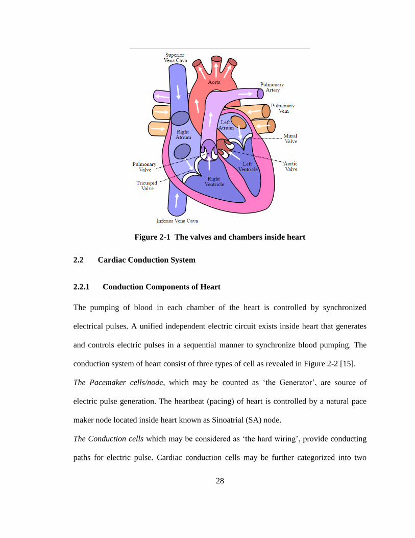
Figure 2-1 The valves and chambers inside heart

2.2 Cardiac Conduction System

2.2.1 Conduction Components of Heart

The pumping of blood in each chamber of the heart is controlled by synchronized

electrical pulses. A unified independent electric circuit exists inside heart that generates

and controls electric pulses in a sequential manner to synchronize blood pumping. The

conduction system of heart consist of three types of cell as revealed in Figure 2-2 [15].

The Pacemaker cells/node, which may be counted as ‘the Generator’, are source of

electric pulse generation. The heartbeat (pacing) of heart is controlled by a natural pace

maker node located inside heart known as Sinoatrial (SA) node.

The Conduction cells which may be considered as ‘the hard wiring’, provide conducting

paths for electric pulse. Cardiac conduction cells may be further categorized into two

29

basic parts as atrial and ventricle conducting cells depending upon their function as

shown in [16].

The Myocardial cells act as actuators, are muscle cells of heart which contract on

receiving electric pulses thus cause the blood pumping action.

Figure 2-2 Cells of Electric Conduction System of Heart [15]

2.2.2 Cardiac Electricity (Action Potential)

First, it is important to understand, how electricity is generated and flow inside heart. The

flow of electric pulse in heart is because of action potential (AP) generated in heart’s

conduction cells. The AP is biological electricity and is not like a normal electric current

that is because of flow of electrons. The AP can be defined as the rapid sequence of

changes in polarity of the excitable cell due to movement of sodium and potassium ions

across the cell membrane when triggered by an electric pulse [17]. In pacemaker cells,

30

this cyclic sequence is automatically self repeated and a pulse is generated after a specific

interval, which defines the heart rate. The AP sequence consists of different

distinguishing stages.

In normal or resting stage, the cardiac cells are polarized in a way that they are more

negatively charged from inside in relation to their outside surface. This polarization is

because of difference in concentration of mainly potassium, sodium, chloride and

calcium ions, however these ions can cross the membrane through channels in it. The

resting AP of cardiac cells is around -80 ~ -90 mV.

Because of some external (or automatic) electric stimulation, the negative ions from the

cardiac cell will flow out and will change polarization of cardiac cell. This process is

known as depolarization. A depolarized cardiac cell can stimulate its neighboring cell to

depolarize and when a row of cell are depolarized sequentially, it cause flow of electric

charge. When cardiac cell is depolarized, it’s potential reaches +10 ~ +30 mV.

Once depolarization is reached, the peak AP (around 30mv) and thereafter the cardiac

cell starts restoring to its rest (normal) state. This process is known as Repolarization.

Plateau is unique for contractile cardiac cell, in which AP is sustained around 0-10 mV

for considerable time duration before start of repolarization.

In some cases, on the termination of repolarization stage, the AP of the cell overshoots

the resting state becoming more negative than the normal polarity. This stage is known as

hyper polarization.

31

2.2.3 The AP Patterns

Contractile cardiac cells are Sodium dependant channel. Sodium channels are voltage

gated channels and are characterized with a Plateau just after repolarization has

started[18]. Plateau of ventricle AP has a longer duration as compared to atrial AP. A

complete cycle of change in AP of contractile cardiac cell is shown in Figure 2-3.

Figure 2-3 Phases of a cardiac AP. "0" (sharp rise in voltage) corresponds to

depolarization, “1” correspond to early repolarization, “2” is plateau, “3”

corresponds to repolarization and “4” is quite (resting) stage

Pacemaker cardiac cells are Calcium channel dependant and have ability to generate

impulsive AP without external trigger thus initiate a rhythmic depolarization/

repolarization cycle automatically[19]. A complete cycle of change in AP of pacemaker

cardiac cell is shown in Figure 2-4 which resembles to a sinusoidal wave.

The AP patterns of various cardiac cells are shown in Figure 2-5. Variations in these

pattern are because of difference in the properties of the cardiac cells and slope/duration

of different phases of these patterns define responses of each type of cardiac cell.

32

Figure 2-4 Phases of a AP of cardiac pacemaker cells. Phase "0" corresponds to

slow diastolic depolarization, Phases “1” and “2” corresponds to termination of

depolarization cycle and plateau, Phase “3” corresponds to slow repolarization and

Phase“4” is termination of depolarization (quite stage)

2.2.4 Refractory Period

The transient period when the cardiac cell is entering from depolarization stage to

repolarization stage, the cardiac cell is in refractory i.e. it cannot respond to new

stimulation and this period is known as Refractory Period. The initial portion of

refractory period is absolute refractory and former portion is relative refractory i.e. a

stronger stimulus if applied can reinitiate the depolarization. In contractile cardiac cell,

phase 1 and 2 are absolute refractory, whereas phase 3 is partial refractory and a strong

signal can initiate depolarization process. A complete cycle of change in AP of

contractile cardiac cell is shown in Figure 2-6.

33

Figure 2-5 The AP patterns of various cardiac cells [15]

Figure 2-6 Depolarization –polarization cycle of Pacemaker Cell

34

2.2.5 Intrinsic Conduction System

The overall conduction system of heart can be grouped into two main categories i.e.

intrinsic and extrinsic conduction system. The intrinsic conduction system of the

heart is an autonomous system which is a combination of different bioelectric

components (cardiac cells) including the Pacemaker node (The Generator), the

conduction cells (the hard wire) and myocardial cells (The actuators). The complete

picture of intrinsic conduction system is shown in

Figure 2-7. Following are major components of intrinsic conduction system.

Figure 2-7 Intrinsic Conduction system of the heart

35

The SA Node. The SA is located in upper right atrium at the verge of

SuperiorVenaCava (SVC) and it plays role of primary pacemaker of the heart. It

initiate the electric stimulus in a rhythm which determines the heart rate (60 beats

per minute under normal conditions).

Inter-nodal and Inter-atrial Pathways. Inter-nodal pathways are links between

SA node and AV node. These pathways spread out through right atrium and cause

the contraction of right atrium. Through these pathways, the electric pulse reaches

the AV node. Inter-atrial pathway is link between SA node and left atrium. This

pathway extends from right atrium to left atrium and carry the electric pulse to left

atrium for its contraction.

AV Node. The AV node is a specialized bundle of tissues that is located between

atrium and ventricular boundary. In a healthy heart, this is the only passage of

stimulus from atrium (upper portion) to ventricle (lower portion). Main role of

AV node is to delay the passage of electric pulse from atrium to ventricle so that

contraction of atrium may be completed before start of ventricle depolarization. It

also plays role of a secondary pacemaker that can initiate a small size electric

pulse (at the rate lower than the initiated by SA node), if pulse from SA node is

blocked.

Bundle of His. Bundle of His is a combination of conduction cells which carries

electric pulse from AV node to the apex of ventricular. It is further divided into

36

two branches for two sides of ventricles; one is right bundle branch (RBB) and

other is left bundle branch (LBB).

Purkinje Fibers. The right/left bundles branches are divided into many thin

pathways known as Purkinje Fibers. These fibers connect electric pulse to the

ventricle muscles and cause depolarization for contraction.

Figure 2-8 The sequence of electric excitation

The stimulus is initiated from SA node, distributed to right/left atrium and causes both

atria to depolarize (contract). After depolarization of both atria, the pulse reaches the AV

node and a conduction delay is enforced in AV node. After a specific delay caused in AV

node, the electric pulse enters the bundle of His and divided into two branches

RBB/LBB. Finally, the electric pulse reaches the Purkinje fibers and depolarizes both the

ventricles. The sequence of electrical excitation of heart is shown in Figure 2-8.

37

2.2.6 Extrinsic Conduction System

The intrinsic conduction system is self autonomous however autonomic nervous system

(ANS) has capability to modify the heartbeat in various circumstances to vary the blood

pumping rate and strength. The external control of heartrate by ANS is known as

extrinsic conduction system as shown in Figure 2-9. It has two subsystem named as

sympathetic and parasympathetic conduction stimulation which, are regulated by the

medulla oblongata. The extrinsic control is the result of a balance between both the

parasympathetic and the sympathetic stimulation system.

Sympathetic conduction stimulation enhances the heart rate under those circumstances in

which fast blood pumping is required e.g. physical fatigue, emotional stress etc. The

functioning of sympathetic stimulation involves thoracolumbar and sympathetic chain

neurons. It simultaneously influence the SA node, AV node and Purkinje

fibers/myocardium as depicted in Figure 2-9.

Parasympathetic conduction stimulation decreases the heart rate via Vagus nerve. It

controls mainly SA node to relax the action potential.

2.3 Normal Sinus Rhythm

If the intrinsic conduction system of the heart remains normal then AP of cardiac cells

follow a sequential rhythm which is initiated and controlled by primary pacemaker of

heart that is sinus node. Under normal conditions, heart rate remains 60-100 bpms and

further change in heart rate is controlled by extrinsic conduction system (regulated by

ANS) as per demand of the body. This rhythmic rise or decrease in heart beat if follow a

regular rhythm then it is also counted as normal. A rhythm is defined as Normal Sinus

38

Rhythm (NSR) if rhythm initiated by SA node, remains regular and heart rate is between

60 to 100 bpm [13, 20-23].

Figure 2-9 Extrinsic conduction system controlled by ANS

2.4 Arrhythmia

If heart rate is not 60-100 bpm (under normal condition) or rhythm is not solely

controlled by sinus node causing irregularity in rhythmic sequence, it is counted as

arrhythmia (abnormal rhythm)[16]. Arrhythmia is categorized in further types based on

location, heart rate and rhythm regularity etc.

2.4.1 Arrhythmia Based on Heart Rate

Based on heart rate, the abnormality is of two types as following.

39

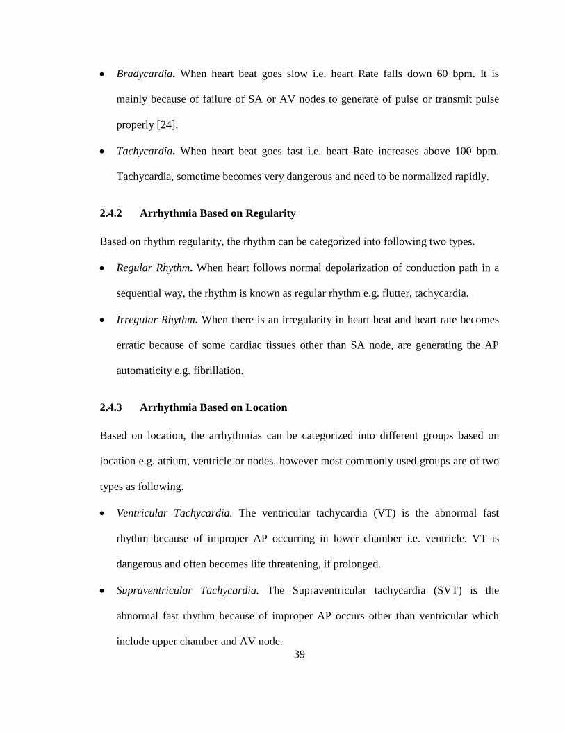
Bradycardia. When heart beat goes slow i.e. heart Rate falls down 60 bpm. It is

mainly because of failure of SA or AV nodes to generate of pulse or transmit pulse

properly [24].

Tachycardia. When heart beat goes fast i.e. heart Rate increases above 100 bpm.

Tachycardia, sometime becomes very dangerous and need to be normalized rapidly.

2.4.2 Arrhythmia Based on Regularity

Based on rhythm regularity, the rhythm can be categorized into following two types.

Regular Rhythm. When heart follows normal depolarization of conduction path in a

sequential way, the rhythm is known as regular rhythm e.g. flutter, tachycardia.

Irregular Rhythm. When there is an irregularity in heart beat and heart rate becomes

erratic because of some cardiac tissues other than SA node, are generating the AP

automaticity e.g. fibrillation.

2.4.3 Arrhythmia Based on Location

Based on location, the arrhythmias can be categorized into different groups based on

location e.g. atrium, ventricle or nodes, however most commonly used groups are of two

types as following.

Ventricular Tachycardia. The ventricular tachycardia (VT) is the abnormal fast

rhythm because of improper AP occurring in lower chamber i.e. ventricle. VT is

dangerous and often becomes life threatening, if prolonged.

Supraventricular Tachycardia. The Supraventricular tachycardia (SVT) is the

abnormal fast rhythm because of improper AP occurs other than ventricular which

include upper chamber and AV node.

40

2.4.4 Arrhythmia Based on QRS Duration (ECG)

One of the popular differentiation of tachycardia is on basis of QRS duration i.e. width of

QRS is narrow or wide.

Narrow QRS. For a normal case, the QRS width remains below 120ms and are

differentiated as ‘Narrow QRS’[25].

Wide QRS. The cases in which QRS width is above 120ms are differentiated as

‘Wide QRS’[26].

2.5 The Origins of Arrhythmia

Once our focus is to classify different arrhythmias, then it is necessary to understand

origin/cause of arrhythmia especially when dealing with IEGMs, which are mostly

localized electric signals. The cause/source behind an abnormality in cardiac rhythm can

be categorized in following basic groups as under [16].

2.5.1 The Pacemaker Problem

The primary pacemaker of heart’s intrinsic system is SA node and secondary is AV node.

Both nodes are further regulated by extrinsic conduction system (ANS). Sometime SA

node generates electric pulse that either is too slow/fast or may not be regular; therefore,

sinus node is responsible for initiating an arrhythmia. Following arrhythmias may be due

to SA node issue.

Sinus rhythm

Sinus bradycardia

Sinus tachycardia

Sick sinus syndrome

41

Figure 2-10 Ventricular ectopic foci

2.5.2 Ectopic Beat

If some cardiac tissues other than the sinus node also achieve AP automaticity and start

generating an electrical activity (usually higher than SA node), will override the sinus

rhythm. Such cases are known as ectopic rhythms. Ectopic foci may be in atrium or

ventricle. Ventricular ectopic foci is depicted in Figure 2-10 and it causes prolongation of

QRS duration in ECG.

2.5.3 Accessory Pathway

The accessory pathway (APs) is undesired conduction path between any of two heart’s

chamber, it may be between atrium to atrium, ventricular to ventricular or atrium to

ventricular. AV node is only one conduction point between atria and ventricle, however

some time an APs is generated which creates abnormality in the rhythmic conduction

cycle.

42

Figure 2-11 Right sided, septal and left sided APs (from left to right) [27]

Based on location of APs, these are further categorized as right sided (from RA to RV),

septal (middle, bypasses AV node) and left sided (from LA to LV) as shown in Figure

2-11. Some of APs are capable of conducting only one way, based on the direction of

conduction these may be further defined as Antegrade APs (conduct from atrium to

ventricle) or Retrograde APs (conduct from ventricle to atrium) [27].

2.5.4 Reentry Mechanism

Reentry is the mechanism, which occurs when a propagating APs wave front does not

terminate after a sequential activation in cardiac conduction path and enter in a loop to re-

excite a portion of cardiac cells in the conduction path (once these cells are out of

refractory period). The majority of arrhythmias are because of Reentry mechanism. In a

reentry mechanism, refractory period of cardiac cells and multiple conduction pathways

are two important factors.

43

Figure 2-12 Local and global reentry

Re-entry tachycardia only occurs when, 1) when there exist dual pathways that is linked

with each other at both sides, 2) the conduction of APs through one pathway is faster as

compared to the other, 3) the faster pathway have longer refractory period as compared to

other pathway. The reentry can be distributed into two sub categories as local reentry and

global reentry as shown in Figure 2-12 [28].

(a) (b)

Figure 2-13 Normal versus reentry mechanism.

44

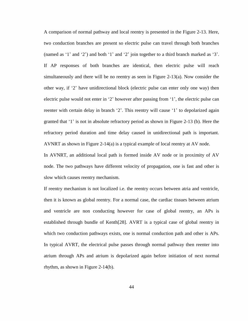
A comparison of normal pathway and local reentry is presented in the Figure 2-13. Here,

two conduction branches are present so electric pulse can travel through both branches

(named as ‘1’ and ‘2’) and both ‘1’ and ‘2’ join together to a third branch marked as ‘3’.

If AP responses of both branches are identical, then electric pulse will reach

simultaneously and there will be no reentry as seen in Figure 2-13(a). Now consider the

other way, if ‘2’ have unidirectional block (electric pulse can enter only one way) then

electric pulse would not enter in ‘2’ however after passing from ‘1’, the electric pulse can

reenter with certain delay in branch ‘2’. This reentry will cause ‘1’ to depolarized again

granted that ‘1’ is not in absolute refractory period as shown in Figure 2-13 (b). Here the

refractory period duration and time delay caused in unidirectional path is important.

AVNRT as shown in Figure 2-14(a) is a typical example of local reentry at AV node.

In AVNRT, an additional local path is formed inside AV node or in proximity of AV

node. The two pathways have different velocity of propagation, one is fast and other is

slow which causes reentry mechanism.

If reentry mechanism is not localized i.e. the reentry occurs between atria and ventricle,

then it is known as global reentry. For a normal case, the cardiac tissues between atrium

and ventricle are non conducting however for case of global reentry, an APs is

established through bundle of Kenth[28]. AVRT is a typical case of global reentry in

which two conduction pathways exists, one is normal conduction path and other is APs.

In typical AVRT, the electrical pulse passes through normal pathway then reenter into

atrium through APs and atrium is depolarized again before initiation of next normal

rhythm, as shown in Figure 2-14(b).

45

(a) (b)

Figure 2-14 (a) AVNRT case through additional local pathway, (b) AVRT case

through accessory pathway [28]

2.5.5 Conduction Blockade

Sometimes undesired delays and hindrance in the flow of AP in intrinsic/extrinsic

conduction system is generated which is referred as blockade in conduction of electric

pulse. The conduction blockade may be partial or complete and can occur anywhere in

the conduction path. Following are main types of conduction block.

SA node block. If SA node is functioning but AP is not able to reach atrial

myocardium and AV node, it is described as sinus block.

AV node block. Any blockade between AV node and right/left bundle branches is

defined as AV block. Different levels of AV blocks are categorized as 1st degree, 2

nd

degree and 3rd

degree Heart Block.

Bundle branch block (BBB). Blockade in any of right or left bundle branches is

referred as left bundle branch block (LBBB) and right bundle branch block (RBBB).

46

2.5.6 Pre-Excitation Syndrome

In pre-excitation syndrome, the electric pulse reaches from atrium to ventricular through

an APs before that the electric pulse reaches through normal conduction path, thus

ventricular gets excited prematurely known as pre-excitation syndrome. Wolff-

Parkinson-White (WPW) and Lown-Ganong-Levine (LGL) syndrome are types of the

pre-excitation syndrome. The comparison between a normal conduction cycle and pre-

excitation case is shown in Figure 2-15; where left sided figure shows a normal cycle and

right side shows pre-excitation syndrome.

Figure 2-15 Normal cardiac cycle on left side versus pre-excited cycle on right side

2.6 Supraventricular Tachycardia

The main focus of this research work is to classify the major arrhythmia related to SVT

therefore, different types of SVT arrhythmia are further elaborated here. SVT

encompasses all arrhythmias which are above ventricular, this includes arrhythmias

47

related to Atrium/SA node and AV node [6]. SVT is a commonly found arrhythmia that

affects over 570,000 people each year. Considering ECG, SVTs are mostly regular and

narrow QRS tachycardia. Majority of the SVTs cases are AVNRT (around 60-70%

cases), AVRT (around 25-30% cases) and AT (5-15% cases) [11]. SVT can be further

grouped into two main categories as under.

2.6.1 Tachycardia from atria

All tachycardia whose source is lying in upper chambers are grouped in this category; it

includes tachycardia related to SA node and both atriums. Following are major

tachycardia rising from atria.

Atrial Tachycardia

In Atrial tachycardia (AT), the rhythm is not fully controlled by SA node rather electric

pulse is initiated within atrium from some other source. The cause may be some ectopic

atrial tissues, which start generating electrical pulses at higher rate than pulse rate

(automaticity) of SA node, thus override the sinus rhythm. In case of AT, the atrial rate

remains between 100-250 bpm [20, 23, 29-31]. In ECG, it is characterized by abnormal

P-wave, regular ventricle rhythm however, ventricular rate may vary from atrial rate [6].

AT may be divided into further categories. For example, focal AT in which, only one

ectopic source of pulses exists whereas in multifocal AT, more ectopic sources exists

which generate pulses. If source of abnormal impulse generation is near or inside AV

which directly conduct to bundle of His without delay however, it is not linked with

reentry mechanism, it is known as junctional ectopic tachycardia [32].

48

Atrial Flutter

In Atrial Flutter (AFL), the tachycardia occurs because of local reentrant circuit

generated inside atria. The local reentry continuously self excites atrial tissues and bring

atria in tachycardia state however, these pulses are not transmitted at the same rate in

ventricle because of refractory period of AV node. Usually pulse reaching ventricles are

in A:V ratio of 2:1 or 3:1. In ECG, it is characterized by saw-toothed F wave, regular

atrial/ventricle rhythm and AV block causing lower ventricular activation rate which may

reach 4:1 [6]. In AFL, the atrial contractions are regular and activation rate remains in

between 230~430 bpm [20, 29, 33-35].

Figure 2-16 Normal atrial activation (regular) versus Atrial Fibrillation (irregular)

Atrial Fibrillations

Atrial Fibrillation (AF) is the type of atrial arrhythmia in which atrial activation rate is

rapid and completely irregular. Difference between a regular rhythm and irregular rhythm

is illustrated in Figure 2-16. Because of irregular atrial rate, the ventricular rate also

49

becomes irregular and sometimes it may become life threatening too. During AF, the

atrial rate can go beyond 600 bpm [36, 37]. In ECG, it is distinguished with the absence

of P-wave, instead of P-wave an vibrating base line is visible, irregular ventricle rhythm

and ventricular activation rate is increased between 100-180 bpm [6].

2.6.2 Tachycardia from AV Node

Mostly arrhythmias related to AV nodes are reentrant tachycardia and two most

commonly observed types are AVNRT and AVRT. Both of these tachycardia have

regular rhythm and narrow QRS complex in majority cases. Description of these

tachycardia is as under.

Atrial-Ventricular Nodal Reentry Tachycardia

AVNRT is because of local reentry and it is one of the most common (60-70% of SVT)

arrhythmia [11]. In a normal conduction system, AV node is the only point of conduction

between atria and ventricle. The significant role of AV node is to impose certain delay in

passing electric pulse from atria to ventricle and only one path should exists, from which

electric pulse passes. In AVNRT case, an abnormality appears in form of two pathways

in AV node as shown in Figure 2-17 and conduction velocity (time delay caused) of both

pathway is not same. One pathway is faster with longer refractory period than the second

pathway, which is slow with smaller refractory period. Out of these two pathways, is

used for normal antegrade conduction whereas the other provides retrograde conduction

and thus a reentry circuit is established. The most (80-90%) common type of AVNRT is

Slow-Fast AVNRT (also known as typical AVNRT) in which slow pathway provides

antegrade conduction and fast pathway provides retrograded conduction as shown in

50

Figure 2-17. In ECG, it is characterized by regular QRS with heart rate increased between

140-250 bpm. In most of cases (typical AVNRT, 90-95%), the P-wave is not visible

because atrial activation occurs almost simultaneously with ventricular activation thus P-

wave hides under the QRS. In some rare cases (atypical AVNRT, 5-10%), P-wave can

also be seen just prior or subsequent of QRS complex [11, 38, 39].

(a) (b)

Figure 2-17 Normal cardiac conduction and AVNRT case

Figure 2-17(a) shows a normal case in which the electric pulse passes early from left side

(fast) pathway and reaches bundle of His early and slow pathway (right) is blocked.

Figure 2-17(b) shows a case of AVNRT in which the left side (fast) pathway is still in

refractory period and blocks the passage of electric pulse; the pulse passes through slow

pathway (right) and reaches bundle of His. The moment the pulse reaches bundle of His,

the refractory period of left side (fast) pathway is over, the pulse reenter through left side

(fast) pathway and reaches RA (known as “echo”) causing atrial tachycardia. In this way,

51

a recurring loop is established which maintains state of tachycardia. The other type of

AVNRT is Fast-Slow AVNRT, which is relatively uncommon (10-20%) [18].

(a) (b)

Figure 2-18 (a) Orthodromic AVRT (retrograde conduction through APs)

(b) Antidromic AVRT (antigrade conduction through APs)

Atrioventricular Reentrant Tachycardia

Another common type of reentrant arrhythmia is AVRT (25-30% of SVT) [23]. The

cause of AVRT is linked with Wolff-Parkinson-White (WPW) Syndrome in which two

separate pathways exist between atria and ventricle; one is the normal pathway through

AV node whereas the other is APs usually generated through bundle of Kenth. The

presence of two pathways provide a reentry mechanism in which electric pulse passes

52

through fastest pathway from atria to ventricle and then reenter from slow pathway back

into atria hence cause tachycardia. Usual heart rate during AVRT remains between 200-

300 bpm. The AVRT can be divided into two main types, orthodromic/antidromic as

shown in Figure 2-18. In Orthodromic AVRT, the conduction occurs antegrade through

AV node and retrograde through APs. In ECG it is characterized by narrow (<120ms)

QRS. It is very common type of AVRT also known as typical AVRT. In Antidromic

AVRT, the conduction occurs antegrade through APs and retrograde through AV node. It

is uncommon type also known as atypical AVRT. In ECG, it is characterized by wide

QRS.

53

CHAPTER 3

ACQUISITION OF CARDIAC ELECTRIC SIGNALS

This chapter describes the basic techniques developed for monitoring and

recording of cardiac electric activity. In a basic clinical diagnosis, cardiac

electric activity is picked from body surface through electrodes and this method is

known as ECG. Although ECG is good enough to observe different types of

abnormality in cardiac conduction system still many characteristics are not

examined by ECG, therefore invasive method is opted as an alternative. In

invasive method, cardiac electric signals are picked directly from inside heart

through electrodes mounted on catheter. The acquired signals are known as

IEGM. IEGM provides complete depth for observation as well as facilitates the

treatment against abnormality. The invasive recording of electrical pulses is

known as EPS. The EPS is done under special protocols that require external

pacing to bring heart in tachycardia state. The key features of both ECG and

IEGM and their relationship with intrinsic conduction system are discussed in

detail in this chapter.

3.1 Electrocardiogram

ECG is recording of heart’s electric activity from body surface of a person. For

monitoring of electric excitation inside the heart, electrodes are placed at various points

in a predefined pattern. A cyclic wave of depolarization initiates from SA node and

culminates at myocardium, passes through conduction pathway that generates relative

positive/negative deflections on surface electrodes. The recorded ECG pattern having

positive/negative deflection is an accumulative effect of heart’s electrical activity as

shown in Figure 3-1.

54

.

Figure 3-1 Accumulative effect of AP of various cardiac conduction cells in a

rhythm

55

Figure 3-2 Complete rhythm of depolarization/repolarization of atrium and

ventricular

The fiducial points observed in an ECG pattern, are given specific names as P, Q, R, S, T

and U waves. The depolarization of atrial muscle (myocardial cells) is deflected as P

wave and depolarization of ventricular muscle are deflected as R wave. Repolarization of

ventricular muscle is deflected as T wave whereas the repolarization of atrial muscles has

small magnitude and overlaps with R wave so it is not visible in ECG. The complete

cycle of depolarization/ repolarization on time scale for a normal heartbeat is shown in

Figure 3-2. The various features/ waveforms description of an ECG signal is given in

Figure 3-3.

Since heart is a three dimensional organ which contains various types of conduction cells

so the exact reflection of electric activity can be understood with combination of many

electrodes (covering three dimensions). Multiple electrodes are required to be placed at

different location on body to depict different views of electrical activity inside the heart.

56

Figure 3-3 The waveform/segment description of an ECG signal

No of electrodes varies depending upon number of views required e.g. 3 leads ECG

(requires 3 or 4 ECG electrodes), 5 leads ECG (require 4 electrodes) and 12 leads ECG

(require 10 electrodes). It can be observed that lead is not same as an electrode; electrode

is a physical contact point from where electrical signals are picked through wires whereas

a lead is a specific view which may be a combination of more than two electrodes makes

a vector measurements [40].

Leads combination may be further categorized as unipolar and biopolar leads. Bipolar

leads are the standard leads that require two electrodes (one considered as positive and

other as negative/reference) to measure an electrical signal variations between them.

Unipolar lead provides additional view of electrical activity, in which signal from an

electrode is picked with reference to a complex negative/reference point that is

combination of two or more electrodes.

57

12 leads ECG is most popular diagnostic ECG combination being followed worldwide.

12 leads have total 12 view combinations made from 10 electrodes. Out of 10 electrodes,

four are limb electrodes named in relation their relative position close to four limbs as

RA (right arm), LA (left arm), RL (right leg) and LL (left leg); six electrodes are the

chest electrodes named as V1-V6 (precordial). The electrode placement on the body is


Figure 3-4 Scheme of 10 electrodes placement (12 leads ECG)

These 12 leads may be categorized into following three sets i.e. limb, augmented limb

and precordial leads. Limb leads are bipolar combination produced from four limb

electrodes (RA, LA, RL and LL). Out of these four electrodes, LL serve as

reference/negative electrode and rest three generate ECG leads with reference to LL.

These leads are named as ‘I’, ‘II’ and ‘III’ as shown in Figure 3-5. Three limb leads

58

provides three different views of the heart in a vertical (frontal) plane. The bipolar limb

lead combinations are produced as following.

I LA RA (3-1)

II LL RA (3-2)

LIII LL A (3-3)

Figure 3-5 The combination of limb leads

Augmented limb leads are unipolar combinations produced from three limb electrodes

(RA, LA and LL). Here one electrode is taken as positive point and combination of

remaining two electrodes makes the reference/negative point. The augmented leads are

named as ‘aVR’, ‘aVL’ and ‘aVF’. This arrangement adds new view angles (vectors) in a

vertical (front) plane as shown in Figure 3-6.

The unipolar augmented limb lead combinations are produced as following. Combining

three limb leads and three augmented limb leads, total six view angles are generated in

vertical plane as shown in Figure 3-7.

59

R2

(LA+LL)aVR A (3-4)

L2

(RA+LL)aVL A (3-5)

LL2

(RA+LA)aVF (3-6)

Figure 3-6 The combination of augmented limb leads

Figure 3-7 The view angles in vertical plane

60

The precordial leads are also unipolar and these covers the horizontal (transverse) plane

meaning that their view angle is perpendicular to vertical (frontal) plane. Each pericardial

electrode is taken as positive terminal to provide six horizontal views whereas the

reference/negative point is generated by averaging the three limb leads RA, LA and LL

(1

3(RA+LA+LL) ) as the center of Wilson triangle. The six unipolar precordial lead

combinations are generated as following.

1V1

3V1 (RA+LA+LL)

(3-7)

1V2

3V2 (RA+LA+LL)

(3-8)

1V3

3V3 (RA+LA+LL)

(3-9)

1V4

3V4 (RA+LA+LL)

(3-10)

1V5

3V5 (RA+LA+LL)

(3-11)

1V6

3V6 (RA+LA+LL)

(3-12)

The six view angles that are generated in horizontal plane from six precordial leads as

shown in Figure 3-8. The complete picture (views) by 12 leads in three-dimensional

domain is shown in Figure 3-9.

61

Figure 3-8 The view angles by six precordial leads in horizontal plane

Figure 3-9 The complete three dimensional view by 12 leads ECG

62

3.2 The Intracardiac Electrogram

The IEGM signals are the localized electrical activity recorded by the electrode catheter

placed directly inside the heart contrary to the ECG in which signals are picked from the

surface of body. ECG represents the vector analysis of electric pulse from different

angles in three domains however, these vectors are sometime unable to provide complete

picture. Therefore, we need to pick localized depolarization being occurred at different

locations of the heart’s conduction circuit. The ECG provides the superimposed picture

of all AP, whereas the IEGM records a timed depolarization/repolarization process for

desired portion of the conduction path. The IEGMs are recorded and analyzed in an EPS

to detect and treat the loci that are source of cardiac arrhythmia [24].

In EP study, specialized electrode catheter is inserted inside the body through some vein

(mostly femoral vein), then catheter is maneuvered to be placed inside the heart at

specific location as shown in Figure 3-10. Usually four catheters are inserted depending

upon the requirement of observation points. The signal from catheters are pre-processed,

amplified and recorded on a computer-based system.

During procedure, it is also required to change the heart-beating rate so an external

stimulus is provided at specific location inside the heart through catheter, under some

special protocols to observe cardiac response. This process is known as Pacing or

Stimulation.

Vital signs such as ECG, blood pressure (BP) and pulse oximetery are also monitored on

independent equipment so that patient safety can be ensured simultaneously. Defibrillator

equipment is also made readily available during EPS to counter abruptly induced

fibrillation state of the heart.

63

Figure 3-10 Catheter placement procedure

Mapping of AP at multiple points inside specific chamber can also be done through

specialized catheter e.g basket catheter, circular catheter etc. The purpose of mapping is

to correlate the electric activities simultaneously at different foci inside the heart.

After determining the cause of problem, it is required to burn the tissues that are

providing undesired conductivity and giving abnormality in heart rhythm. For this

purpose, RF (300-750 kHz) is delivered to the desired locus through the catheter that

produces heat and burn the desired tissues. This process is known as Ablation.

64

Figure 3-11 EP catheter electrode

3.3 Cardiac Catheterization for EP Study

3.3.1 IEGM Catheters

Catheter is a flexible insulated thin cable that is inserted into the heart. Catheters are of

different types and shapes. It has a handle/control at its rear end that is used to maneuver

it through blood veins and heart’s chamber, as shown in Figure 3-11. First role of catheter

is diagnostic however, these are also used for pacing and ablation purpose [41].

Multiple electrodes are mounted on a catheter. Catheter may be configured in unipolar or

bipolar mode. In bipolar mode, two adjacent electrodes are used as a pair as shown in

Figure 3-12. Bipolar electrodes are preferred for recording of localized AP activity. Inter

electrode spacing between two electrodes as well as between two pair of electrodes are a

design feature specified for different applications; a 2-5-2mm electrode spacing means

that gap between two +/- pair of electrodes is 2mm whereas gap between a pair to another

pair is 5mm.

65

Figure 3-12 Bi-polar catheter configuration

3.3.2 Basic Catheter Configuration

During an EP study, multiple catheters are placed simultaneously however, the basic EP

procedure requires following standard catheter configuration. These catheters are named

on basis of their location of employment as shown in Figure 3-13.

HRA Catheter. HRA (high right atrium) catheter is placed with the right atrium wall

near the SVA to record atrial activity initiated by SA node. Usually it is a quadripolar

type (contains 4 electrodes).

RVA Catheter. RVA (right ventricular apex) catheter is placed as close as possible

with the apex of right atrium. It records the electric activity of purkinje fibers and

myocardium of right ventricle. Usually it is also quadripolar type.

CS Catheter. CS (coronary sinus) catheter is placed in coronary sinus vein. It is used

to record the AP of the left side (LA and LV) of the heart. A steerable decapolar

catheter (contains 10 electrodes) is preferred.

66

HIS Catheter. His catheter is located near His bundle (located superior side of

tricusipid annalus) to record AP activity of AV node and of His bundle. A curved tip

steerable quadripolar catheter is preferred.

http://www.theeplab.com/B-The-Members-Center/E000-EP-Procedures/B-Catheter-Placement/EB00-Catheter-

Placement.php

Figure 3-13 Basic configuration of HRA, His, RVA and CS catheters and their

fluroscopic view in left anterior oblique (LAO) position

3.3.3 Basic Features of IEGMs

In one rhythm of ECG, ‘P’, ‘QRS’ and ‘T’ etc waves are taken as feature that reflects

accumulative depolarization/repolarization of atria/ventricle. In IEGMs, we record

localized depolarization near the electrode catheter (in bipolar configuration) so we get an

http://www.theeplab.com/B-The-Members-Center/E000-EP-Procedures/B-Catheter-Placement/EB00-Catheter-Placement.php

http://www.theeplab.com/B-The-Members-Center/E000-EP-Procedures/B-Catheter-Placement/EB00-Catheter-Placement.php

67

electric pulse when a depolarization wave front passes near the electrode catheter. In

IEGM, we have three distinct features named as following:

A-wave. It represent atrial depolarization and can be seen good in HRA catheter and

small amplitude A-wave can also be seen on His and CS catheters.

H-wave. It represent the depolarization in bundle of His. It is a small amplitude signal

and can be seen only in His catheter.

V-wave. It represent ventricular depolarization and posses a strong amplitude in RVA

catheter and it can also be seen good in His catheter.

Correlation between IEGM waves and ECG feature is shown in Figure 3-14 which

illustrate ‘A’,’V’ and ‘H’ waves in relation to normal ECG signal. In IEGM, the ‘A’ and

‘V’ wave features are observed on more than one pair of electrodes (bipolar) which

depicts the time gaps/durations of the electric pulse traveling from one point to other. The

sequence/time gap of a feature at different locations provides the evidence of conduction

path being followed and thus depicts the abnormality if any.

Figure 3-14 Correlation between IEGM and ECG features

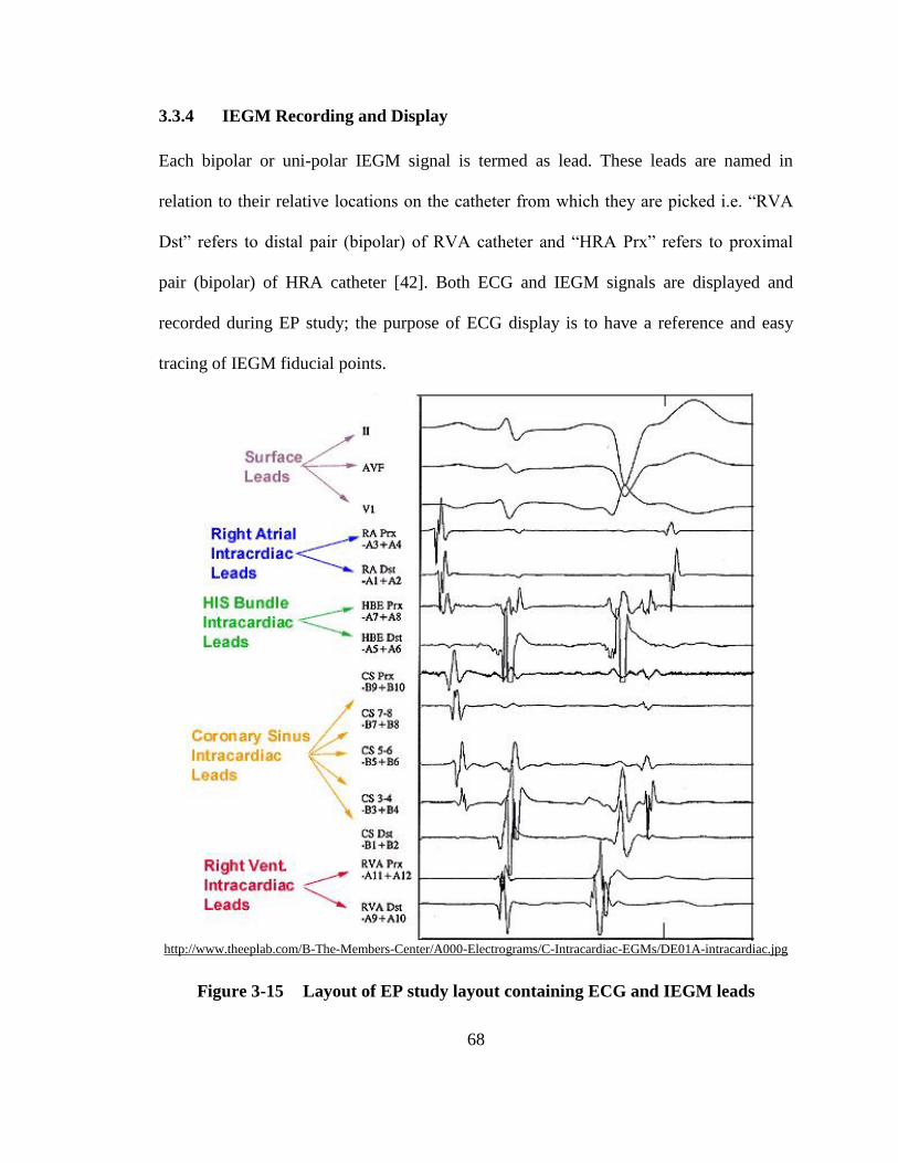
68

3.3.4 IEGM Recording and Display

Each bipolar or uni-polar IEGM signal is termed as lead. These leads are named in

relation to their relative locations on the catheter from which they are picked i.e. “RVA

Dst” refers to distal pair (bipolar) of RVA catheter and “HRA Prx” refers to proximal

pair (bipolar) of HRA catheter [42]. Both ECG and IEGM signals are displayed and

recorded during EP study; the purpose of ECG display is to have a reference and easy

tracing of IEGM fiducial points.

http://www.theeplab.com/B-The-Members-Center/A000-Electrograms/C-Intracardiac-EGMs/DE01A-intracardiac.jpg

Figure 3-15 Layout of EP study layout containing ECG and IEGM leads

http://www.theeplab.com/B-The-Members-Center/A000-Electrograms/C-Intracardiac-EGMs/DE01A-intracardiac.jpg

69

http://www.theeplab.com/B-The-Members-Center/A000-Electrograms/C-Intracardiac-EGMs/DE01G-intracardiac4.jpg

Figure 3-16 Propagation of ‘A’ wave sequentially from RA to CS leads

Usually 2-3 different ECG leads selected by electrophysiologist, are displayed at the top

and then 8-12 different IEGM leads are displayed subsequently. It is preferred that order

of leads display is in a sequence in which electric pulse flow in normal conduction path.

The preferred layout contains first ECG leads, then HRA leads, His leads, CS leads and

http://www.theeplab.com/B-The-Members-Center/A000-Electrograms/C-Intracardiac-EGMs/DE01G-intracardiac4.jpg

70

RVA leads are displayed as shown in Figure 3-15. This figure shows the complete set of

waveforms that is available during basic EP study. This sequence facilitates to correlate

different features. For example, we can locate ‘A’ wave first in HRA catheter prior to ‘P’

wave in ECG, then it is progressively visible in His and CS catheter with delayed in time

axis because of natural conduction sequence; however ‘A’ is not visible in RVA catheter

as shown in Figure 3-16. ‘H’ wave is very small and is visible between A & V in HIS

catheter only.

Figure 3-17 Appearance of ‘A’-wave and ‘V’-wave

71

The V signal is most dominating and can easily first identified in RVA distal prior to R

wave in ECG, and progressively appear (delayed in time axis) in the other leads from

bottom to top as can be seen in Figure 3-17.

3.3.5 Programmed Electrical Stimulation

To observe the AP properties of the heart, external pacing (stimulation) at faster rate is

carried out and corresponding response is observed. In programmed electrical stimulation

(PES), a sequence of electric pulses are given in a specific pattern that overdrives the

natural pacing sequence of heart and tachycardia is induced. Activation pattern in

tachycardia, its initiation/termination and response to extra stimuli is observed closely.

The rate of pacing is also increased gradually under a specific protocol to study the

conduction and refractoriness of cardiac cells.

Figure 3-18 Antegrade Versus Retrograde Pacing

Stimuli are given in a combination of multiple stimulus (typically 6-8 pulses) in a

sequence known as drive train. Amplitude of stimulus should be typically 2-4 times of

72

diastolic threshold and have width 1-3ms (millisecond). Based on the location , pacing is

done in following two ways, as shown in Figure 3-18 [18].

Antegrade pacing. Pacing in atrium is carried out close to SA node (but not at SA

node) through HRA catheter.

Retrograde pacing. Pacing in ventricular is carried out through RVA catheter or

sometime His catheter. It provides insight of bottom up electrical conduction paths.

73

CHAPTER 4

PRE-PROCESSING OF INTRACARDIAC SIGNALS

Heart’s electrical activity when picked through invasive or non-invasive

electrodes have very low amplitude, thus IEGM/ECG is highly vulnerable to

noise. For accurate extraction of ECG/IEGM features, the noise removal is very

important, however removing noise from the IEGM/ECG signal may also distort

valuable contents therefore, optimal filter designing is required to avoid loss of

vital signal information. In this chapter, noise removal of PLI and EMG noises

are taken care off.

4.1 Scope of Pre-Processing

During EP study, the onset of IEGM features i.e. A, H and V waves are used to classify

the arrhythmia. The classification accuracy greatly depends upon signal to noise ratio

(SNR) of the IEGM. Therefore it is required to pre-process an IEGM signal such that

fiducial points remain preserved as much as possible. The pre-processing of an IEGM

includes removal of PLI, EMG and in some cases BLW as well. This is followed by

marking of fiducial points to extract features and finally arrhythmia classification as


Figure 4-1 Stages of Arrhythmia Classification Algorithm

74

Filtration requirement of different kind of cardiac signal for an EP study is as shown in

Table 4-1 [42].

Table 4-1. Filtration requirement for ECG/IEGM signals

ECG/IEGM High Pass Filter Low Pass Filter

Surface ECG 0.1Hz 100 Hz

Bi-polar IEGM 30 Hz 300 Hz

Uni-polar IEGM 1Hz 300 Hz

Uni-polar IEGM

(unfiltered) 0.1 Hz 400 Hz

Filtration requirement for bipolar signal is from 30-300 Hz and for unipolar signal is 1-

300 Hz [15, 42]. The useful features of ECG/IEGM may be spoiled if proper frequency

ranges are not taken care while performing pre-processing[43]. In most of cases, bipolar

IEGM configuration is used, so frequency range should be applied accordingly. Figure

4-2 illustrates the importance of inappropriate frequency ranges. In Figure 4-2(a),

ECG/IEGM both signals are filtered with the frequency range of 0.5-300 Hz which is not

suitable for a bipolar IEGM lead and will distort/override the small H wave. In Figure

4-2(b), ECG/IEGM both signals are filtered with the frequency range of 30-300 Hz which

is good for IEGM but inappropriate for ECG signal thus compromise the ECG features.

Figure 4-2(c) shows the appropriate way of pre-processing in which ECG signal is

filtered with 0.5-300 Hz and IEGM signal is filtered with 30-300 Hz and feature

information remains preserved.

75

(a) (b) (c)

Figure 4-2 Effect of inappropriate frequency band selection during pre-

processing [15].

Similarly if a notch filter is employed for removal of PLI, the ringing effect is generated

which distort the valuable information present in IEGMs as shown in Figure 4-3.

Figure 4-3 Effects of a notch filter for removal of PLI [15].

76

4.2 Power Line Interference

PLI and its harmonics is the most devastating noise even if the IEGM/ECG equipment is

operated on battery. The problem is further complicated when frequency of PLI is not

static, making the conventional notch filter completely ineffective. IEGM signals are

further complicated with presence of harmonics of PLI as well. The frequent variations in

PLI frequency poses a serious problem and it is further enhanced because of involvement

of multiple power sources being used in health care centers (in Pakistan), which include

1) the electric power provided from main grid, 2) the uninterruptable power supply (UPS)

and 3) generator power sources. Moreover, the frequency of main grid also varies largely

because of fluctuation of load on main grid. In this section, an intelligent adaptive noise

rejection filter has been proposed which tracks and eliminates PLI as well as its

harmonics. The proposed system can estimate the frequency of PLI and tune the adaptive

filter for precise elimination of PLI as well as its harmonics without requirement of an

auxiliary reference input. The proposed system is based on recursive state space model,

inherited with less computational complexity and performs well in a non-stationary

environment. The proposed system responds well to the ongoing variations in amplitude

and frequency of PLI present in IEGM signals. The proposed system does not require any

reference signal for tracking the PLI and its harmonics, it is capable to self adjust its

tracking frequency.

4.2.1 Literature Review - PLI

IEGM having a wider frequency band of interest (1-300 Hz) is more sensitive to various

kinds of noises; out of which PLI is most disruptive disturbance. For the case of IEGM

77

signals, the filtration of PLI and its harmonics should be more accurate and precise. An

electrocardiogram signal is considered to be high quality if it contains PLI noise below

0.5% of the electrocardiogram’s peak amplitude [44].

A variety of methods has been used for removal of PLI from the cardiac signals. The

most conventional methods is the use of a notch filter. The notch filter are implemented

into two configurations i.e. finite impulse response (FIR) or infinite impulse response

(IIR), however IIR notch filters are preferred because their filter order is much smaller as

compared to counterpart FIR. The notch filter has constrain of ringing effects and large

transient response and it cannot perform well when power system has large variations in

PLI frequency [45].

As an alternate of notch filter, many authors have proposed different adaptive filtration

techniques. Concept of adaptive noise cancellation (ANC) was introduced by Widrow et

al. and was applied by J.R. Glover for PLI cancellation [46, 47]. ANC requires PLI as a

reference signal for adaptation by the adaptive filters like Least Mean Square (LMS) and

Recursive Least Square (RLS) [48], [49]. Moreover, the coupling of reference input also

cause increase in the cost of medical devices and is not always available especially in

portable equipments.

Later on, a technique known as Adaptive Sinusoidal Interference Canceller (ASIC) was

proposed, in which frequency of PLI is presumed to be a fixed whereas amplitude and

phase are two adaptive parameters of the system [50], [51]. Another approach is proposed

by Bazhyna in which he isolates the linear/ non-linear segments in electrocardiogram and

then linear segment is used to estimate the interference [52]. A limitation of this approach

is that non linear segments and linear segments need to be identified prior to PLI

78

detection thus makes the system more complex. Koseeyaporn et al. use geometric

representation and PLI as a combination of sine and cosine waves [53]. They adjust the

amplitude of reference signal by varying the amplitude/phase of sine and cosine waves

using LMS algorithm. Islam S. Badreldin et al. presented the adaptive removal of PLI

noise and its harmonics from cardiac signal without sampling an external power line

reference [54], [55].

In this work, an adaptive configuration is applied which does not require a reference

signal to track and eliminate the PLI present in the IEGM signal effectively [56]. While

dealing with IEGM signals, we need to filter out PLI interference as well as its

harmonics. To cater for the PLI frequency variation, an online frequency estimation

technique is implemented which dynamically tunes adaptive filter with ongoing changes

in frequency thus making its functioning highly effective.

4.2.2 Problem Formulation

The desired frequency spectrum of a standard bipolar IEGM lead is 30-300 Hz and in

some cases electrophysiologist may prefer frequency band 0.1-400 Hz therefore,

sampling frequency of IEGM signal must be 1 kHz or greater [57, 58].

Ideally, a 50 Hz AC power system contains only fundamental frequency component of 50

Hz but practically, integral multiples of fundamental frequency known as harmonics are

also present. Generally only odd harmonics are present in the power system because of

half wave symmetry property [59]. For a standard ECG signal, we are interested in

frequency band of 1-80Hz, therefore we need to tackle only the 1st harmonic i.e.,

fundamental frequency however, for an IEGM signal, we need to take care of 3rd

and 5th

79

harmonics of PLI as well. Therefore, in case of 50 Hz power system, we need to track

and eliminate 50, 150, and 250 Hz frequency components simultaneously. In case larger

frequency band of IEGM lead is desired, the higher odd harmonics of PLI (i.e. 350, 450

Hz etc) may be taken into account.

As a case study, a raw IEGM signal recorded at National Institute of Heart Diseases

(NIHD) Pakistan, which is sampled at 2000 samples/sec, is selected as shown in Figure

4-4. The IEGM waveform shown in Figure 4-4 is in raw form i.e. it contains PLI along

with its harmonics and other noises as well. To observe frequency components of this

raw IEGM, its frequency spectrum is shown in Figure 4-5. The frequency spectrum

shown in Figure 4-5 clearly depicts the presence of fundamental frequency and odd

harmonics of PLI; it is also evident that there is no presence of even harmonics. For

IEGM, we apply low pass filter at 300 Hz which means that we need to tackle 1st

(fundamental frequency), 3rd

, and 5th

harmonics only.

IEGM signal corrupted with PLI and its harmonics can be represented by

[ [[ ] ] ] IEGM PLIy n x n x n (4-1)

where [ ]y n is IEGM signal corrupted by PLI, [ ]IEGM

nx is the pure IEGM signal and

[ ]PLI nx is the PLI noise consisting of 1st, 3

rd, and 5

th harmonics of PLI and can be

represented by

1 1 3 3 5 5[ ] sin( ) sin(3 ) sin(5 )

PLIx n n n n (4-2)

80

Where n is the discrete time index, ω is the normalized PLI frequency defined as

L s= 2 f / f ; Lf is the fundamental PLI frequency, sf is sampling frequency. 1α , 3α , 5α

are amplitudes of the 1st , 3

rd, and 5

th PLI harmonics respectively. 1φ , 3φ , and 5φ are phases

of the 1st , 3

rd, and 5

th PLI harmonics respectively.

0 0.5 1 1.5 2 2.5 3 3.5 4

-1

-0.8

-0.6

-0.4

-0.2

0

0.2

0.4

0.6

0.8

1Corrupted IEGM Signal

Time (seconds)

No

rmali

zed

Am

pli

tud

e

Figure 4-4 IEGM data sampled at 2 kHz (No signal filtration/processing applied)

The state space model encompassing 1st, 3

rd, and 5

th harmonics of PLI is derived as

following:

Let the 1st harmonic i.e. 1 1

sin( )n be the first state of a sixth order state space

system and the second state is also 1st harmonic with a phase shift of / 2 as following.

81

2

1 1 1

1 1

sin( )

cos( )

[ ]

][

n

n

x n

x n

(4-3)

0 100 200 300 400

-60

-40

-20

0

20

40

60

80

100

120Frequency Spectrum of HRECG

Frequency (Hz)

Ma

gn

itu

de

(d

B)

Fundamental power frequency

3rd harmonic5th harmonic

7th harmonic

Figure 4-5 Frequency spectrum of Raw IEGM signal

Similarly, the 3rd

and 4th

states represent 3rd

harmonic of PLI.

4

3 3 3

3 3

sin(3 )

cos(3 )

[ ]

[ ]

n

n

x

x

n

n

(4-4)

And the 5th

and 6th

states represent 5th

harmonic of PLI.

6

5 5 5

5 5

sin(5 )

cos(5 )

]

]

[

[

n

n

x n

x n

(4-5)

82

Using trigonometric identities, we may rewrite the six states as

1 1 1

1 1 1

3 3 3

3 3 3

5 5 5

5 5 5

1

2

3

4

5

6

[ ]

[ ]

[ ] 3 3

[ ] 3 3

[ ] 5 5

[ ] 5 5

sin cos cos sin

(cos cos -sin sin )

sin cos cos sin

(cos cos -sin sin )

sin cos cos sin

(cos cos -sin sin )

n

n

n

n

n

n

x n n

x n n

x n n

x n n

x n n

x n n

(4-6)

Equation (6) may be rewritten as

1 1

1 1

3 3

3 3

5 5

5 5

1

2

3

4

5

6

cos sin

cos

3 3

3 3

5 5

5 5

sin

cos-sin

sincos sin

cos-sin cos

sincos sin

cos-sin cos

0 0 0 0[ ]

[ ] 0 0 0 0

[ ] 0 0 0 0

[ ] 0 0 0 0

[ ] 0 0 0 0

[ ] 0 0 0 0

x

x

x

x

x

x

n

n

n

n

n

n

(4-7)

Defining initial condition at n = 0, we have

1 1 1 1 3 31 2 3

4 3 3 5 5 5 55 6

[0] [0] [0]

[0] [0] [0]

x = α sinφ , x = α cosφ , x = α sinφ

x = α cosφ , x = α sinφ , x = α cosφ (4-8)

Putting initial conditions and considering states at n = 1 in (7) we get

1 1

2 2

3 3

4 4

5 5

6 6

cos sin

cos

3 3

3 3

5 5

5 5

-sin

cos sin

-sin cos

cos sin

-sin cos

0 0 0 0[1] [0]

[1] [0]0 0 0 0

[1] [0]0 0 0 0

[1] [0]0 0 0 0

[1] [0]0 0 0 0

[1] [0]0 0 0 0

x x

x x

x x

x x

x x

x x

(4-9)

83

Similarly, starting with initial states, we can recursively update states at any time

0n > .

The generalized form of (4-9) can be re-written as:

1 1

2 2

3 3

4 4

5 5

6 6

cos sin

cos

3 3

3 3

5 5

5 5

1]

1] -sin

1] cos sin

1] -sin cos

1] cos sin

1] -sin cos

0 0 0 0[ [ ]

[ [ ]0 0 0 0

[ [ ]0 0 0 0

[ [ ]0 0 0 0

[ [ ]0 0 0 0

[ [ ]0 0 0 0

x n x

x n x

x n x

x n x

x n x

x n x

n

n

n

n

n

n

(4-10)

Here

cos sin

cos

3 3

3 3

5 5

5 5

-sin

cos sin

-sin cos

cos sin

-sin cos

0 0 0 0

0 0 0 0

0 0 0 0

0 0 0 0

0 0 0 0

0 0 0 0

is state

transition matrix, which is marginally stable i.e. all its eigen values lie on the unit circle.

This transition matrix represents the state space model of 1st, 3

rd, and 5

th harmonics of

PLI, which is dependent on only one parameter i.e. normalized fundamental PLI

frequency.

4.2.3 Methodology

A state space recursive least square (SSRLS) adaptive filter configuration as shown in

Figure 4-6 is proposed for elimination of PLI from IEGM signal.

84

Proposed layout suggests the use of SSRLS as adaptive noise canceller, in which 1st, 3

rd,

and 5th

harmonics of PLI are adaptively tracked by SSRLS filter and then subtracted from

corrupted IEGM signal to get pure IEGM. The overall filtration performance depends

upon the tracking accuracy of the SSRLS filter. The performance of tracking depends on

the selection of frequency for tracking whereas the frequency of PLI is not constant

therefore, we need to estimate the fundamental frequency of PLI and tune the SSRLS

filter accordingly. For monitoring the frequency of PLI, an intelligent DFT (Discrete

Fourier Transform) is applied. A batch of data is processed to estimate fundamental PLI

frequency and the estimated frequency is fed to adaptive filter. The signal is fed to

adaptive filter through a delay block because of inherent delay involved in frequency

estimation process.

Figure 4-6 Proposed layout for elimination of PLI and its harmonics

85

The proposed combination allows us to adaptively adjust itself to any change in

frequency and tracks the amplitude/phase of 1st, 3

rd, and 5

th harmonics of PLI for

selective filtration without distorting the other frequency components of IEGM signal.

The description of each block is given in subsequent sections.

4.2.4 Frequency Estimation

Fundamental frequency of PLI is estimated prior to SSRLS filtration which is used for

tracking 1st, 3

rd, and 5

th harmonics by the SSRLS filter. For estimation of power line

fundamental frequency, an intelligent DFT algorithm is employed which provides high

resolution frequency estimation [56]. Intelligent DFT works on the assumption that

fundamental frequency of PLI dominates in the frequency band of 45-55 Hz of PSD

(Power Spectral Density) of a PLI corrupted IEGM. This assumption meets the criteria of

a good quality electrogram to have PLI component less than 0.5% of its peak amplitude

[44]. The intelligent DFT algorithm is intelligent in a sense that it provides high

resolution frequency estimation with less number of operation counts as well as performs

well with small data window size which makes it feasible for online frequency

estimation. DFT of N points sequence is calculated as.

1 2 /.

0

N j kn NX x enk n

(4-11)

where N defines the size of data window selected for DFT and xn refers to nth discrete

signal entity of selected window. k is the discrete frequency index defined by

( / ) sk N f f , where f is the frequency in hertz and sf is sampling frequency.

86

For the case of diverging PLI frequency, our requirement is to observe online PLI

frequency changes precisely. Since maximum variation in PLI frequency is limited to

10% , we need to focus on the frequency band of 45-55Hz (for 50 Hz power system) to

search for fundamental PLI frequency. Fast Fourier Transform (FFT) is commonly

employed method for PSD estimation, which transforms the complete frequency

spectrum (i.e. 2

sf), thus makes it inefficient for our requirement. Moreover FFT cannot

provide high resolution frequency estimation without zero padding when smaller window

size is selected for transformation into frequency domain as discussed in detail in [56].

On the other hand we can calculate DFT against desired discrete frequencies lying in

frequency band of 45-55Hz by direct application of (11). The frequency resolution

achieved through DFT can be calculated by

/df f (4-12)

where df is the frequency resolution, f is the desired frequency band and is the

number of frequency bins. If we increase the frequency resolution, we need to increase

the number of frequency bins thus require more computations to perform. Our desired

f is 45-55 Hz. To have frequency resolution of 0.01Hz through basic DFT algorithm,

we require 1,000 frequency bins.

In intelligent DFT algorithm, the frequency resolution is enhanced with less cumulative

number of the frequency bins. Here df is gradually increased by narrowing down f

gradually. Resultantly we achieve higher frequency resolution with much reduced

computational effort. No zero padding is used for enhancement of frequency resolution.

87

Application of Hanning windowing is useful in order to overcome the spectral leakage

issues. Functioning of intelligent DFT algorithm is depicted in flow chart shown in

Figure 4-7.

Figure 4-7 Intelligent DFT - Flow chart.

88

The search of 49.36 Hz frequency in three stages by the proposed algorithm is shown in

Figure 4-8, where frequency resolution of 0.01 Hz is achieved with only 30 frequency

bins (in 45-55 Hz frequency band) in three stages. In first stage, we select 10 frequency

bins, it will provide frequency resolution ( df ) of 1 Hz and out of these 10 frequency

bins, only two bins with highest magnitude are chosen to select a frequency band for next

stage. In next stage, we have to deal with bandwidth of 1 Hz and recalculate the DFT

with 10 frequency bins thus we achieve frequency resolution of 0.1 Hz. Therefore, df is

enhanced 10 times in each stage by just doubling the computation. Resultantly the df of

0.01 Hz is achieved in three stages with 30 frequency bins instead of 103 frequency bins

hence computational complexity is reduced manifolds.

Figure 4-8 Working of intelligent DFT: The resolution of PLI frequency

estimation is gradually enhanced in each subsequent stage and a resolution of

0.01Hz is achieved by performing DFT of 30 frequency bins only in three stages.

Enhancement of frequency estimation resolution in three stages.

89

A comparison between FFT, DFT and proposed intelligent DFT techniques has been

carried out in order to compare operation counts and time lag (delay caused because of

samples, if no zero padding is applied). Let 2sf KHz and desired 0.01df Hz . The

computational complexity and number of samples required to estimate the PLI signal in

the band of 45-55 Hz, through each technique, are given in Table 4-2. Proposed

algorithm achieves a explicit reduction in operation counts as compared to DFT and FFT.

Table 4-2 FFT, DFT and intelligent DFT comparison for PLI frequency search

with 0 01.df Hz

Parameters FFT DFT Intelligent DFT

No of samples

required (N)

/ sN f df

=2x105

10 cycles of 50Hz

PLI = 400

10 cycles of 50 Hz PLI

= 400

Delay involved 100 seconds 0.2 seconds 0.2 seconds

Frequency

selection range

( f )

f =1000

Hz

(by default

/ 2sf )

f =10 Hz

110Hzf (1

st iteration)

21Hzf (2

nd iteration)

30.1Hzf (3

rd iteration)

No of

frequency bins

( )

N =

2x105

/f df =103

110 (1

st iteration),

210 (2

nd iteration),

310 (3

rd iteration)

1 2 330

No of

operation count

(Computation

complexity)

22 log ( )N N

=7.05X106

N

= 4.0X105

N

=1.2X104

90

The high resolution frequency estimation is achieved with a small batch of data without

any zero padding. However to ensure a consistent outcome of intelligent DFT, minimum

size of data batch (N) is restricted to contain at least 10 cycles of the frequency to be

observed. For the case of PLI (50 Hz) frequency estimation with sampling frequency of 2

kHz, a batch of 500-1000 samples is an appropriate choice. Having a larger batch size

will cause lesser variation in outcome however, at the cost of delay incurred for

collection of complete batch.

For online monitoring of variations in PLI frequency, the intelligent DFT can be

implemented on successive data segments as sliding DFT [60]. If the selection of next

data window is done with a jump (gap) by number of samples equal to length of window,

the connective windows are non-overlapping.

Use of non-overlapping windows technique requires less number of windows over the

entire data length; renders minimum computational effort however, observation delay of

full window length is faced. To reduce observation time delay, the consecutive windows

can be overlapped; resultantly total numbers of windows over entire data length will

increase. Since computational effort of intelligent DFT algorithm is much reduced

therefore for each new window, intelligent DFT is reapplied without using the results of

previous (partially overlapped) window. The increase in computational cost will be only

in term of increased number of windows; conversely observation delay will also be

reduced in same proportion. Using the half window overlap configuration is an

appropriate choice.

91

Figure 4-9 (a) Non-overlapping window with observation delay of N samples, (b)

Half window overlapping with observation delay of N/2 samples

Suppose at discrete time instance n, a batch of data ( )x n consisting of N samples is

selected as following

- 1 - 2 -1( ) { , ,...., , }

n N n N n nx n x x x x (4-13)

For the case of half window overlap configuration means that the connective data

window slides by N/2 samples and is defined as

2 2 2 22 - 1 - 2 -1

( ) { , ,...., , }

N N N N

N

n n n nnx x x x x

(4-14)

The observation delays for the case of non overlapping window as well as half window

overlapping cases are shown in Figure 4-9.

92

Figure 4-10 Sliding window DFT and delay caused.

4.2.5 Delay Block

To counter the delay caused because of batch processing of DFT algorithm, a delay

block is used before adaptive filtration system as shown in Figure 4-6. The initial delay

caused is equal to size of the data window; thereafter the amount of delay (D) depends on

the number of samples we slide between two consecutive windows (overlap). The delay

caused by half window overlap configuration is shown in Figure 4-10. For example if

window size is the 500 samples and half window overlap configuration is used, the initial

delay will be 500 samples and thereafter delay will be 250 samples. The ongoing delay

can be reduced by increasing window overlap i.e. if window size of 500 samples is in ¾

overlap configuration, the delay will be of 125 samples.

93

4.2.6 SSRLS Adaptive Filter

The SSRLS is an adaptive filter which works in state space framework [61]. Let the

unforced discrete time state space system be described as follows.

[ 1] [ ] [ ]

[ ] [ ] [ ] [ ]

x n A n x n

y n C n x n v n (4-15)

where [ ]x n is the state vector at time index n and [ ]A n is the system matrix. [ ]y n is the

desired output vector, [ ]C n is output matrix and [ ]nv is output disturbance vector which

may be considered as observation noise.

Comparing (4-10) and (4-15), we have

1 2 3 4 5 6[ ] [ ] [ ] [ ] [ ] [ ][ ] T

x n x n x n x n x n x nx n (4-16)

and

cos sin

cos

3 3

3 3

5 5

5 5

-sin

cos sin

-sin cos

cos sin

-sin cos

0 0 0 0

0 0 0 0

0 0 0 0

0 0 0 0

0 0 0 0

0 0 0 0

A

(4-17)

SSRLS filter estimates the states ˆ[ ]x n on each observation [ ]y n . The working of

SSRLS algorithm is summarized here.

The estimated state vector and estimated output is given by

ˆ[ ] [ ] [ ] [ ]

ˆ ˆ[ ] [ ]

x n x n K n n

y n Cx n (4-18)

94

where ˆ[ ]x n is a posteriori state estimate and [ ]x n is the a priori state estimate,

defined as

ˆ[ ] [ -1]x n Ax n (4-19)

[ ] n is the prediction error, taken as

[ ] [ ] - [ ] n y n y n (4-20)

[ ]y n is the predicted output state defined as

ˆ[ ] [ -1]y n CAx n (4-21)

[ ]K n is the observer gain defined as

-1

[ ] [ ] T

K n n C (4-22)

[ ] n is recursively updated by

- -1

[ ] [ -1] T T

n A n A C C (4-23)

where λ is the forgetting factor which defines the selectivity of adaptive filter

and its value lies in the range of 0 < λ < 1 . The value of λ close to 1 means highly

selective filter i.e. it have narrow bandwidth.

Working of SSRLS adaptive filter is shown in Figure 4-11. The tracking of 1st,

3rd

, and 5th

harmonics of PLI are desired, therefore we choose C vector in (14) as

1 0 1 0 1 0C (4-24)

With this C vector, the estimated output ˆ( )y n will be as follows.

[ ] [ ] [ ]1 3 5

ˆ[ ] n n ny n x x x (4-25)

95

Figure 4-11 Working of SSRLS.

Comparing (4-3), (4-4), (4-5), and (4-25) we have

1 1 3 3 5 5sin( ) sin(3 ) sin(5 )ˆ[ ] n n ny n (4-26)

The output ˆ[ ]y n is the estimated PLI noise [ ]PLI

nx as defined in (4-2). Subtracting

ˆ[ ]y n from corrupted IEGM signal [ ]y n gives us pure IEGM signal [ ]IEGM

x n .

[ [] [ ] ] IEGM

x n y n y n (4-27)

For initialization, regularization or delayed recursion techniques are the choices; we

choose the delayed recursion technique because of superior convergence properties[61].

In order to start the recursion of SSRLS, we need to define the initial estimate of states

x̂[0] and initial observer gain K[0] at time k = 0 . The SSRLS filter starts with these

arbitrary values and then adaptively estimates the states of the system.

96

During the initial period, the selectivity of proposed adaptive filter is not taken very high

i.e. λ 0.95 because the value of is not certain. During the initial period, is also

estimated simultaneously by intelligent DFT. After the initial period, the SSRLS is tuned

with correct value of and thereafter λ is enhanced for highly selective narrow band

tracking. The wider band tracking during initialization, allows us to track the surrounding

frequency components of arbitrary for initial period.

4.2.7 Results

For testing /demonstration of proposed algorithm, an IEGM signal acquired from

National Institute of Heart Diseases (NIHD) at sampling rate of 2000 samples/second is

selected as test signal. This test signal is then normalized. Pure sample IEGM signal is


0 0.2 0.4 0.6 0.8 1

-1

-0.8

-0.6

-0.4

-0.2

0

0.2

0.4

0.6

0.8

1IEGM Test Signal

Time (seconds)

No

rmali

zed

Am

pli

tud

e

Figure 4-12. IEGM Test signal with sampling rate of 2000 samples/sec.

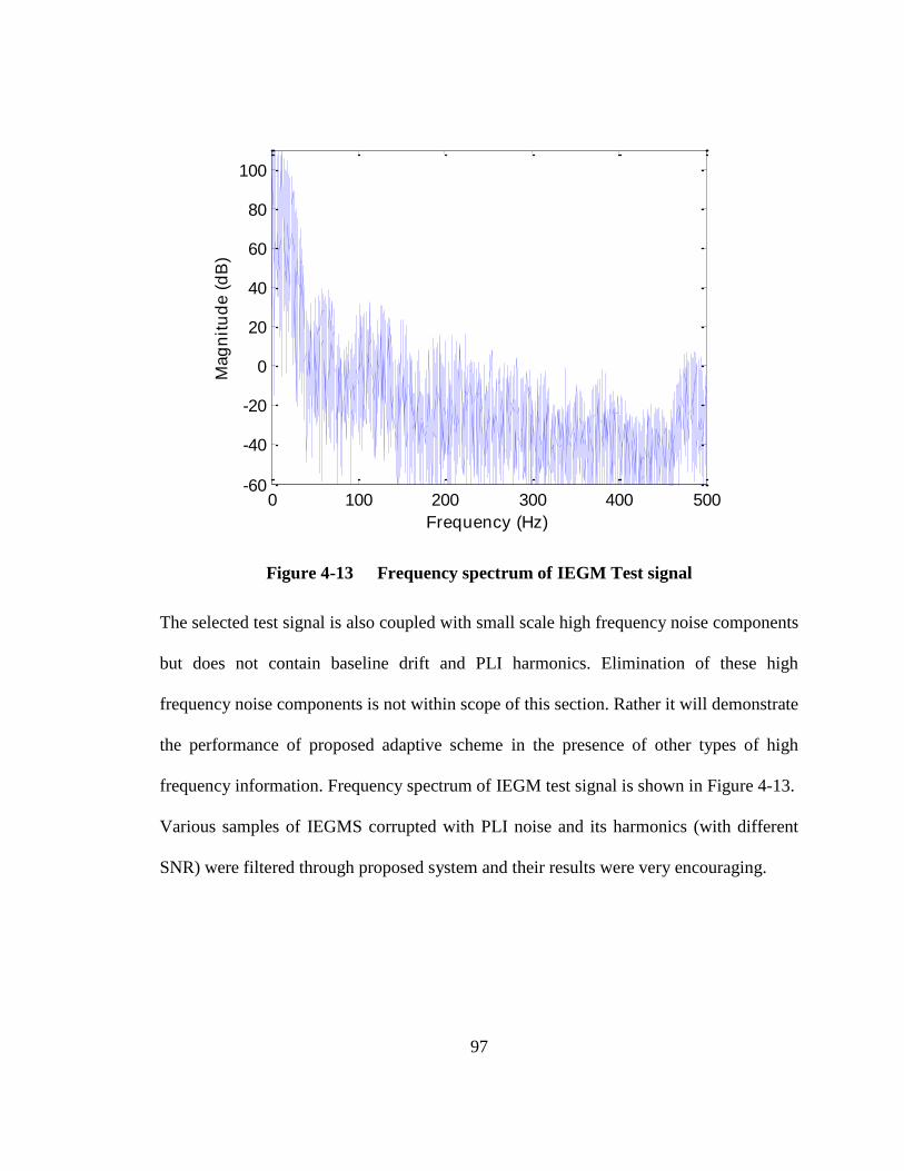
97

0 100 200 300 400 500-60

-40

-20

0

20

40

60

80

100

Frequency Spectrum of HRECG Test Signal

Frequency (Hz)

Mag

nit

ud

e (

dB

)

Figure 4-13 Frequency spectrum of IEGM Test signal

The selected test signal is also coupled with small scale high frequency noise components

but does not contain baseline drift and PLI harmonics. Elimination of these high

frequency noise components is not within scope of this section. Rather it will demonstrate

the performance of proposed adaptive scheme in the presence of other types of high

frequency information. Frequency spectrum of IEGM test signal is shown in Figure 4-13.

Various samples of IEGMS corrupted with PLI noise and its harmonics (with different

SNR) were filtered through proposed system and their results were very encouraging.

98

0 5 10 15 20 25 30 35 40 45

-0.1

-0.05

0

0.05

0.1

0.15

PLI Harmonic Components and Composite Signal

Time (mil iseconds)

No

rmali

zed

Am

pli

tud

e

1st Harmonic

3rd Harmonic

5th Harmonic

Composite PLI

Figure 4-14 The scale of 1st, 3

rd, and 5

th Harmonics of PLI in composite test signal

For a case study, PLI noise having fundamental frequency L

f = 50.38 Hz and its odd

harmonics is formulated with following proportion.

1 1 1sin 3 5

10 50 100sin sin

PLIx (4-28)

where L s= 2 f / f and 2sf KHz .

Relative amplitudes of 1st, 3

rd, and 5

th harmonics of PLI and resulting composite PLI

signal PLIx are shown in Figure 4-14.

99

0 0.5 1 1.5

-1

-0.5

0

0.5


Time (seconds)

No

rmali

zed

Am

pli

tud

e

Figure 4-15 PLI corrupted IEGM signal

0 100 200 300 400 500

-50

0

50

100

Frequency Spectrum of Simulated IEGM

Frequency (Hz)

Mag

nit

ud

e (

dB

)

Figure 4-16 Frequency spectrum of IEGM signal corrupted with 1st, 3

rd, and 5

th

harmonics of PLI.

The composite PLI is mixed with pure IEGM signal to construct a PLI corrupted IEGM

signal as defined in (1) and its SNR value is 7.46 dB (decibels). The corrupted IEGM

signal is shown in Figure 4-15. The frequency spectrum of corrupted IEGM signal is

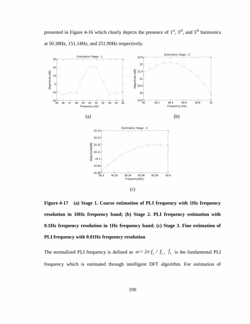
100

presented in Figure 4-16 which clearly depicts the presence of 1st, 3

rd, and 5

th harmonics

at 50.38Hz, 151.14Hz, and 251.90Hz respectively.

45 46 47 48 49 50 51 52 53 54 55-20

-10

0

10

20

30

Frequency (Hz)

Mag

nit

ud

e (

dB

)

Estimation Stage - 1

50 50.2 50.4 50.6 50.8 51

19.5

20

20.5

21

21.5

22

22.5

Frequency (Hz)

Mag

nit

ud

e (

dB

)


(a) (b)

50.3 50.32 50.34 50.36 50.38 50.422.08

22.09

22.1

22.11

22.12

22.13

22.14

Frequency(Hz)

Mag

nit

ud

e(d

B)


(c)

Figure 4-17 (a) Stage 1. Coarse estimation of PLI frequency with 1Hz frequency

resolution in 10Hz frequency band; (b) Stage 2. PLI frequency estimation with

0.1Hz frequency resolution in 1Hz frequency band; (c) Stage 3. Fine estimation of

PLI frequency with 0.01Hz frequency resolution

The normalized PLI frequency is defined as L s= 2 f / f , Lf is the fundamental PLI

frequency which is estimated through intelligent DFT algorithm. For estimation of

101

fundamental frequency of PLI, window size of 500 samples is selected and Hanning

windowing is applied to reduce spectral leakage.

0 1 2 3 4 5 6 7 8 950

50.1

50.2

50.3

50.4

50.5

50.6

50.7

50.8

50.9

51

Time (seconds)

Fre

qu

en

cy (

Hz)

Online Frequency Estimation

Actual fundamental frequency of PLI

Frequency estimation by intell igent DFT

Figure 4-18 Frequency estimation through proposed scheme. Maximum frequency

deviation remains within ±0.02 Hz of actual frequency.

Intelligent DFT algorithm is implemented with selection of 10 frequency bins ( ) in each

stage and starting with frequency band ( )f of 45-55Hz, we achieve frequency resolution

( )df of 0.01Hz in three stages. Results of first three stages are shown in Figure 4-17.

Estimation of fundamental frequency of PLI through intelligent DFT is shown in Figure

4-18. The frequency is estimated in range of 50.36 ~ 50.40 Hz against actual frequency of

50.38Hz and the maximum deviation from actual frequency remains within ±0.02 Hz.

102

For initialization of SSRLS adaptive filter, delayed recursion technique is

selected. SSRLS is a recursive filter, therefore we need to start with arbitrary values of

certain parameters which include , λ , ˆ[0]x and [0] . Initial values of these

parameters are set as λ =0.95, 0.1= rad/sample, ˆ[0] [0 0 0 0 0 0]T

x , and

[0] 0.1T

CI C which is equivalent as

1.1 0 1 0 1 0

0 0.1 0 0 0 0

1 0 1.1 0 1 0

0 0 0 0.1 0 0

1 0 1 0 1.1 0

0 0 0 0 0 0.1

[0]

Initial observer gain [0]K is determined by [0] . Tracking of composite PLI signal by

SSRLS filter during initialization period is shown in Figure 4-19. After the initial period,

the SSRLS is tuned with correct value of estimated by intelligent DFT and the state

transition matrix is modified. Simultaneously value of λ is also raised to 0.99 to enhance

tracking performance. Filtration error calculated as the difference between clean IEGM

signal and Filtered IEGM signal is shown in Figure 4-20, which is negligible after

initialization period.

103

0.15 0.2 0.25 0.3 0.35 0.4 0.45 0.5

-0.4

-0.2

0

0.2

0.4

0.6

Time (seconds)

No

rmali

zed

Am

pli

tud

e

PLI tracking during initial ization

Actual PLI component

PLI tracked by SSRLS

IEGM signal without PLI

Figure 4-19 Tracking of SSRLS adaptive filter during initialization period

0 0.1 0.2 0.3 0.4 0.5 0.6 0.7 0.8 0.9 1 1.1 1.2

-0.3

-0.2

-0.1

0

0.1

0.2

0.3

0.4

0.5

0.6

Time (seconds)

No

rmali

zed

Am

pli

tud

e

Fi l tered IEGM Signal

Fil tered IEGM Signal

Error

Initial ization Period

Figure 4-20 Filtered IEGM signal after initialization

104

50 100 150 200 250 300-50

0

50

100

Frequency (Hz)

Ma

gn

itu

de

(d

B)

Frequency Spectrum of tracked signal

Frequency spectrum of tracked signal

Frequency spectrum of corrupted HRECG

(a)

50 100 150 200 250 300-50

0

50

100

Frequency (Hz)

Ma

gn

itu

de

(d

B)

Frequency Spectrum of Filtered Signal

Frequency spectrum of filter output

Frequency spectrum of clean signal

(b)

Figure 4-21 (a) Frequency spectrum of tracked signal. (b) Frequency spectrum of

filtered IEGM signal with comparison to a clean IEGM signal.

105

0 2 4 6 8 10

-1

-0.8

-0.6

-0.4

-0.2

0

0.2

0.4

0.6

0.8


Time (seconds)

No

rmali

zed

Am

pli

tud

e

Figure 4-22 Raw IEGM signal corrupted with PLI harmonics and other noises.

0 100 200 300 400 500

-50

0

50

100

Frequency Spectrum of Raw HRECG

Frequency (Hz)

Ma

gn

itu

de

(d

B)

Figure 4-23 Frequency spectrum of raw IEGM signal showing presence of 1st, 3

rd,

5th

, 7th

and 9th

harmonics of PLI.

106

0 100 200 300 400 500-100

-50

0

50

100

Frequency Spectrum of Filtered HRECG

Frequency (Hz)

Ma

gn

itu

de

(d

B)

Figure 4-24 Frequency spectrum of filtered IEGM, only 1st, 3

rd and 5

th harmonics

are eliminated.

The frequency spectrum of PLI tracking signal is shown in Figure 4-21 (a) which reflects

precise tracking of 1st, 3

rd, and 5

th harmonics of PLI by proposed system. The frequency

spectrum of 10,000 samples (5 sec) of filtered IEGM signal is shown in Figure 4-21 (b)

which shows complete elimination of 1st, 3

rd, and 5

th harmonics of PLI frequency.

To ascertain the functioning of proposed filter in real situation, IEGM signals which

contains PLI harmonics were also tested and output performance was same as was

observed with simulated test signal. A case of 10 seconds segment of IEGM signal

corrupted with PLI along with its harmonics and other noises is shown in Figure 4-22.

The frequency spectrum of corrupted signal is shown in Figure 4-23 which clearly

depicts the presence of PLI and its harmonics. Since the scope of this section is limited to

elimination of 1st, 3

rd, and 5

th harmonics of PLI only, the filtration of harmonic

107

components of PLI above 300 Hz and other noises are not handled during testing. The

frequency spectrum of filtered IEGM signal is shown in Figure 4-24. It can be observed

that 1st, 3

rd, and 5

th harmonics of PLI are completely eliminated whereas higher harmonic

components are still present. All frequency components above 300 Hz including PLI

harmonics can be filtered out through low pass filter in another stage.

4.2.8 Performance Analysis

Performance of proposed filter is compared with the notch filter. For our case study we

need three cascaded 2nd

order IIR notch filters for elimination of 1st, 3

rd, and 5

th

harmonics of PLI. First of all, it is assumed that PLI frequency is known and remains

fixed at 50.38 Hz. Therefore notch filters are tuned at Lf (50.38 Hz), 3x

Lf (151.14 Hz),

and 5xLf (251.90 Hz) to eliminate 1

st, 3

rd, and 5

th harmonic of PLI respectively. The

quality factor of these notch filters is taken as 100 for better characteristics. The clean

IEGM signal, corrupted IEGM signal, the output of notch filter and the output of

proposed filter are presented in Figure 4-25. It is evident that transition period of notch

filter is much greater than of the SSRLS adaptive filter.

Having the input SNR level of 7.46 dB, the output of proposed system achieves SNR

level of 31.46 dB whereas output of notch filter has the SNR level of 18.55 dB. The

performances of both filters were checked at various SNRs and difference in the output

SNRs of both filters was akin. For a case of high SNR where input SNR is 27.46 dB,

output SNRs of proposed system and notch filter are 49.72 dB and 37.73 dB respectively.

Similarly, for a case of low SNR where input SNR is 1.434 dB, the output of proposed

system and notch filter have SNRs 24.56 dB and 12.75 dB respectively.

108

-1

-0.5

0

0.5

1

No

rmali

zed

Am

pli

tud

e

0.5 1 1.5 2 2.5 3 3.5 4 4.5-1

-0.5

0

0.5

1

Time (seconds)

-1

-0.5

0

0.5

1Filtration comparison

Clean IEGM

-1

-0.5

0

0.5

1

PLI corrupted signal

SSRLS fi l ter output

Notch fi l ter output

Figure 4-25 Filtration quality of SSRLS adaptive filter and notch filter.

Let us now compare the performance of both the filters when there is a step change in

amplitude of PLI. The effect of step change in amplitude of PLI is produced by abruptly

increasing the amplitudes of 1st, 3

rd, and 5

th harmonics of PLI then it is mixed with pure

IEGM. The results of step change in PLI amplitude are shown in Figure 4-26 which

shows that SSRLS filter quickly adapt to track changes in amplitude and thus filter it out

109

from IEGM where as notch filter combination is unable to handle it fast and IEGM signal

remains corrupted for long duration. With this configuration, the SNR level of input

signal is 2.52 dB and the output of proposed system achieves SNR level of 27.81 dB

whereas output of notch filter has the SNR level of 17.07 dB.

-1

-0.5

0

0.5


Clean IEGM

-1

-0.5

0

0.5

1


-1

-0.5

0

0.5

1

No

rmali

zed

Am

pli

tud

e


0.5 1 1.5 2 2.5 3 3.5 4 4.5 5 5.5-1

-0.5

0

0.5

1

Time (seconds)


Step Change

Figure 4-26 The filtered outputs of proposed system and notch filters with step

change in amplitude of PLI disturbances.

110

-0.5

0

0.5


Clean IEGM

-0.5

0

0.5

1


-0.5

0

0.5

1

No

rmali

zed

Am

pli

tud

e


0.5 1 1.5 2 2.5 3 3.5 4 4.5-1

-0.5

0

0.5

1

Time (seconds)


Figure 4-27 The filtered outputs of proposed system and notch filter with ramp

change in amplitude of PLI disturbances.

To observe ongoing continuous change in amplitude of PLI, effect of ramp

increase in amplitude of composite PLI signal is produced and results are presented in

Figure 4-27. In this case, the SNR level of input signal is 3.13 dB and the output of

111

proposed system achieves SNR level of 37.56 dB whereas output of notch filter has the

SNR level of 22.48 dB. The zoomed-in view of filtered outputs of SSRLS adaptive filter

and notch filter are presented in Figure 4-28. Note the variations in clean IEGM signal

are because of presence of high frequency components. Regardless of changing

amplitude of PLI, the output of proposed system matches with the minor variations of

pure IEGM signal whereas notch filter exhibits greater error.

5.08 5.1 5.12 5.14 5.16 5.18-0.06

-0.04

-0.02

0

0.02

0.04

0.06

0.08

Time (seconds)

No

rmali

zed

Am

pli

tud

e

Fi l tered Signal Comparison

Clean IEGM signal



Figure 4-28 The zoomed-in output comparison of proposed system and notch filter

with ramp change in amplitude of PLI disturbances.

Now let us compare the response of both the filters when PLI frequency variation occurs.

For simulation of frequency variation, fundamental frequency of PLI is changed from

50.38Hz to 51.75Hz at 5.3 seconds of IEGM data. The result of intelligent DFT algorithm

applied with 50% sliding window configuration is shown in Figure 4-29.

112

SSRLS adaptive filter is instantly tuned with the updated frequency estimation by

intelligent DFT. For having comparison of notch filter with SSRLS adaptive filter, notch

filter is also run in adaptive manner with continuous update of notch frequencies. The

results of both SSRLS adaptive filter and notch filter are shown in Figure 4-30 and it is

observed that SSRLS adaptive filter swiftly converge to change in frequency whereas

transition time of notch filter is much larger as compared to SSRLS adaptive filter. In this

case the SNR level of input signal is 7.46 dB and the output of proposed system achieves

SNR level of 22.14 dB whereas output of notch filter has the SNR level of 15.95 dB.

0 1 2 3 4 5 6 7 8 9 1049

49.5

50

50.5

51

51.5

52

52.5

53Estimated Frequency

Time (seconds)

Fre

qu

en

cy (

Hz)

Actual fundamental frequency of PLI

Frequency estimated by Sliding window DFT

Initial ization Period

Figure 4-29 Frequency estimation by intelligent DFT with sliding window

configuration

Comparing the results of SSRLS adaptive filter and notch filter, it can be straight way

concluded that performance of SSRLS adaptive filter is much better than the notch filter

combination. However, computational complexity of SSRLS adaptive filter is high as

113

compared to IIR notch filter because of involvement of matrices operation in state space

model therefore execution speed of SSRLS adaptive filter is less as compared to notch

filter.

-0.5

0

0.5

1

Filtration comparison

Clean IEGM

-0.5

0

0.5

1


-0.5

0

0.5

1

No

rmali

zed

Am

pli

tud

e


0.5 1 1.5 2 2.5 3 3.5 4 4.5-1

-0.5

0

0.5

1

Time (seconds)


Change in PLI frequency

Figure 4-30 The filtered outputs of proposed system and notch filters with change

in frequency of PLI.

114

The proposed system can be extended to filter 7th

and 9th

harmonics of PLI from

corrupted IEGM signals if we need frequency band is up to 500 Hz.

4.2.9 Summary – PLI Noise Removal

This research section implements a state space based adaptive filter for tracking and

elimination of PLI and its harmonics from IEGM signal. The SSRLS adaptive filter is

used which is recursive in nature. Unlike Kalman filter, SSRLS filter does not require

process/observation noise covariance for accurate tracking of PLI and its harmonics. The

PLI tracking accuracy of proposed filter depends on two parameters only; first is tuning

frequency and the second parameter is forgetting factor, which effects the bandwidth of

the tracking signal. For high selectivity, we can choose a higher value of forgetting factor

but at the same time, the high selectivity can affect the performance if tuning frequency is

not accurate. Power line frequency remains fluctuating therefore continuous update of the

tuning frequency is desired. For estimation of ongoing power line frequency, an

intelligent DFT based system has been incorporated which continuously estimates and

updates the adaptive filter’s tuning frequency. The proposed system does not require any

reference signal for tracking the PLI and its harmonics; it is capable to self adjust its

tuning frequency for highly precise filtration of 1st, 3

rd and 5

th harmonics of PLI. Separate

tracking of all harmonic components enables the proposed system to work well in non-

stationary environment without distorting underlying IEGM signal.

4.3 Base Line Wander

Base line wandering (BLW) is a low frequency noise (0.15 – 0.3 Hz) produced by

respiration, perspiration, body movements or poor electrode contact and distort ECG

115

interpretation [62]. Presence of BLW in ECG imposes problems in identification of

isoelectric line, wrong ST segment analysis, misreading of T peak as R peak, and

merging of P waves in BLW noise. It is normally represented as an additive sinusoidal

component (0.15 - 0.3 Hz) to ECG signal [57]. Many researchers have used AHA

standards and applied high pass digital FIR/IIR filters to remove BLW from ECG [63-

69]. Also a wide range of other BLW removal techniques are available in literature

including Moving Average filters [70-72], Median filter [73, 74], wavelet transform [75-

78], empirical mode decomposition [79] and adaptive filtering [80-83]. Since BLW can

be represented in term of a sinusoidal signal, so the same technique as discussed in

previous section (i.e. removal of PLI) can also be applied successfully for removal of

BLW. The overall scheme does not require reference signal for ECG de-noising.

While dealing with IEGMs, filtration requirement for bipolar signal is from 30-300 Hz

and for unipolar signal is 1-300 Hz [15, 42]; BLW being a low frequency noise (0.15 ~

0.3 Hz), does not distort the IEGM signals. Therefore, removal of BLW has not been

presented in this research work.

4.4 Electromyographic Noise

Electromyographic Noise (EMG) is a broad spectrum, randomized noise, which is

commonly observed in both ECG and IEGM [84, 85]. The EMG noise generally

considered as high frequency noise and its frequency range varies in between 1~10000

Hz and possesses 0.1~10 mV magnitude depending upon rate of movement and strength

of muscle activity [86]. In some literature the lower frequency range of EMG noise has

been taken above 10 Hz [87, 88]. Accuracy of classification algorithms is directly related

116

to the extent of noise removed from these signals. In clinical EPS, suitable selection of

high frequency noise removal technique during preprocessing of IEGMs is vital so that

most of the noise is removed without loss of signal characteristics.

4.4.1 Literature Review - EMG

In clinical EPS, one encounters signal subjected to various types of noise. Since ECG and

IEGMs both represent electrical activity of the heart, filtering techniques applied on the

ECG signals can be adapted and applied to the IEGMs while taking care of the desired

frequency ranges [89]. Noise sources that corrupt the clinical EP signals are similar to

those affecting the ECG signals. EMG noise removal techniques for electrical signals of

the heart range from simple FIR filters to IIR filters, moving average filters to windowing

methods and median filters [63, 90, 91]. Adaptive filtration has also been applied for

removal of EMG noises [92, 93]. Wavelet filters and Savitzky-Golay (S-G) filters have

also been employed for the purpose of noise removal [94-96].

The amplitude of some of IEGM features are very small and while filtration of high

frequency noise, there is chance of losing such features. For high frequency filtration, S-

G filter provides us a suitable choice to be applied on ECG and IEGM signals [94].

4.4.2 Proposed Method

The acquired IEGMs are first processed for removal of PLI distortion as discussed in

previous section thereafter, EMG noise is taken care off. For removal of EMG noise, S-G

filter is proposed [97]. The S-G filter is a type of FIR filter that performs smoothing

operation by using least-square polynomial fitting technique. For pre-processing of

IEGMs, S-G filter is advantageous because it retains the height and width of the

117

waveform peaks and its impulse response is symmetric so frequency response is purely

real [97]. In essence, they perform a least squares fit of the signal in such a way that

computing the fitting polynomial) of degree N at a central point in the data batch is

equivalent to convolving the input with a fixed impulse response. The fitting polynomial

is given as,

0

( )

N

k

k

k

p n a n (4-29)

where k

a are the polynomial coefficients. The luxury of using S-G filters is that the fitting

polynomial depends on the size of the data batch (2M+1) and degree (N) of the

polynomial but is independent of the actual values of input signal. This eliminates the

need for calculating the polynomial for each new data set and the polynomial is

calculated just once at the beginning of the smoothing operation [97].

Figure 4-31 Filtered IEGM signal from proposed method.

118

The proposed method was tested for noise removal from EMG corrupted IEGMs

acquired from AFIC/NIHD databank and results were successful. The S-G filter designed

for smoothing of IEGMs in this approach had M=7 and N=2. Figure 4-31 represents the

input and output of the S-G filter implemented on an IEGM signal. The magnified graph

of the result is presented in Figure 4-32. It shows how S-G filters preserve the height of

the H wave which is most critical in all characteristic features of IEGMs (i.e. A, H and V

waves). The result shows that the filtered output does not contain EMG noise whereas the

H wave is preserved for clear identification.

Figure 4-32 Zoomed view of S-G Filtered IEGM signal shows preservation of ‘H’

feature.

119

4.4.3 Comparison with other Filtering Techniques

The basic requirement of an ideal EMG filter suitable for IEGMs, can be defined as

following.

Size of characteristic waves in term of its peak and width are retained in the data.

The cutoff frequency of EMG filter ( as a low pass filter) must be above 400 Hz to

preserve genuine data content[27].

Taking into account these desired properties, the performance of S-G filter has been

compared with various filters on the same set of IEGMs data. Comparison is given as

following:

Figure 4-33 EMG removal from IEGM through Moving Average filter

4.4.3.1 Moving Average Filter

The moving average (MA) filter is a simple, fast processing, FIR low pass filter which is

commonly used for smoothing of a data array. Seventh order MA filter has been selected

120

for comparison purpose. The result of the filtered signal is shown in Figure 4-33. It shows

that MA filter removes the high frequency noise however, H waves has been

compromised such that the H wave in IEGM signal has been expanded in time which will

produce inaccuracy in temporal relationship of characteristic waves. Hence, MA filter is

not an appropriate option.

Figure 4-34 EMG removal from IEGM through IIR Filter

4.4.3.2 IIR Filter

Unlike FIR filter, an IIR filter has infinite response i.e. its impulse response does not

become exactly zero after passing a certain time. Although IIR filter is computationally

simple because of its lower order in comparison of FIR filter for same specifications of

filter however, on the other hand it also has stability and phase distortion issues. In our

comparison, a Butterworth low pass IIR filter is applied for removal of EMG noise from

121

IEGMs. Results are shown in Figure 4-34 and it shows that ringing effect are generated in

the filtered output where sharps transitions were present and did not perform satisfactory

smoothing.

4.4.3.3 Median Filter

The median filter determines the output value as the median of the data array. The

outcome of the median filter are shown in Figure 4-35 and it shows that it completely

overwhelm the small amplitude H wave, hence it is also not a suitable option as well.

Figure 4-35 EMG removal from IEGM through Median Filter

4.4.4 Summary – EMG noise

Having comparison of S-G filter with other filters, it can be easily concluded that S-G

filter removes the EMG noise and smoothens the IEGMs with minimum distortion in

height and width of characteristic waves as compared to other filtration options.

122

CHAPTER 5

TEMPORAL FEATURES OF INTRACARDIAC SIGNALS

In conventional clinical EPS, the key concept behind arrhythmia detection

algorithms is the temporal relationships of the feature points within the

electrograms under consideration. Classification of arrhythmias based on IEGMs

requires the analysis of the onsets of characteristics waves i.e. Atrial

depolarization wave (A), His bundle depolarization wave (H) and Ventricular

depolarization wave (V). Accuracy of arrhythmia detection depends upon

accurate detection of the feature points.

5.1 Literature Review

After pre-processing, the next phase of arrhythmia detection algorithm is the feature

detection. The automated feature detection and classification of IEGM signals is rarely

found in literature, however one may refer to different techniques applied on ECG signals

for feature detection [98-100]. Feature detection may be based on morphological,

template, statistical, time domain, frequency domain or hybrid technique (i.e.

combination of two or more methods). Morphological/template features are commonly

used in ECG signals [101-105]. The ECG signal is a superimposed signal of multiple AP

happening simultaneously at different locations of the heart whereas the IEGMs represent

mainly the localized AP and the shape of the characteristic waves in IEGMs differs

largely from one patient to another, so morphological analysis on these signals is not a

suitable method. ECG feature-point detection methods extract the P, QRS, and T wave

features. QRS complex detection methods involving slope of the complex, pattern

123

recognition method and pole-zero models with certain modifications may bear fruitful

results in feature detection for IEGMs [106-108]. Envelope detection can be used for the

purpose of feature point detection [100]. Arrhythmia classifiers have been developed

which make use of the properties of the cardiac signals defined in time-domain and

frequency-domain [109]. In clinical EPS, doctors use timing information of the

characteristic A, H and V waves to manually diagnose the disease and that is why time-

domain analysis forms the foundation of this research. This approach uses adaptive

thresholding techniques in combination with envelope detection for the localized

detection of feature points.

5.2 Data Collection

The acquisition of SVT arrhythmia relevant IEGM dataset was a difficult task because

the complete range of gold standard dataset was not available on Physionet or any other

authentic resource. Therefore, the majority of required Patient’s dataset was collected

from AFIC/NIHD Pakistan and few from MIT Physionet database as available [12].

These dataset was verified from expert electrophysiologist for the specific type of

arrhythmias and then it was referred as gold standard for research work.

The AFIC/NIHD dataset was recorded in bipolar configuration through 2-5-2 mm

catheters to avoid far field ventricular activity. It consists of 3 x ECG leads and 9 x

IEGMs bipolar signals as depicted in Figure 5-1. The recorded IEGMs are in the range of

-5mV to +5mV, which are digitized at 2 KHz sampling rate with 16 bits precision.

The MIT dataset was recorded in bipolar configuration from different positions of the

right atrium using 2-5-2 mm catheters sampled at 1000 samples/sec. The MIT dataset

consist of 3 x ECG leads and 5 x IEGMs bipolar signals, as depicted in Figure 5-2.

124

I

AFIC/NIHD Patients Dataset

aVF

V1

HRA

HISD

HISP

CS 9-10

CS 7-8

CS 5-6

CS 3-4

CS 1-2

0 1 2 3 4 5

RVA-D

Time(sec)

Figure 5-1 5 sec segment of AFIC dataset containing 3xECGs and 9xIEGMs

125

II

Physionet Patients Dataset

V1

aVF

CS 1-2

CS 3-4

CS 5-6

CS 7-8

0 1 2 3 4 5

CS 9-10

Time(sec)

Figure 5-2 The MIT dataset containing 3xECGs and 5xIEGMs

5.3 Methodology

Multiple catheters are inserted in the human heart for EP studies. For the scope of this

research, the focus remains mainly on the recordings from three catheters labeled as the

HRA, His and RVA as shown in Figure 5-3. Further, the IEGMs of CS catheter can be

used as reference for locating the side of APs, which has been recommended as future

126

work. While dealing with IEGMs, the A, V and H waves, their temporal relationship and

inter feature intervals helps to differentiate among arrhythmias [18]. The automated

differentiate among various SVT through IEGM signals can be done by marking A, V

and H waves. Out of all IEGM leads, the His lead is the only lead where we can mark all

the three features i.e. A,V and H waves on single lead directly. However, the marking of

H-wave is crucial and difficult as well as need extra caution.

External stimulation/pacing is applied to drive the heart at faster rate so as to observe the

cardiac response under specific protocols. The scheme of temporal features detection

from IEGMs is illustrated in Figure 5-4.

Figure 5-3 Catheters Arrangement for SVT arrhythmia detection

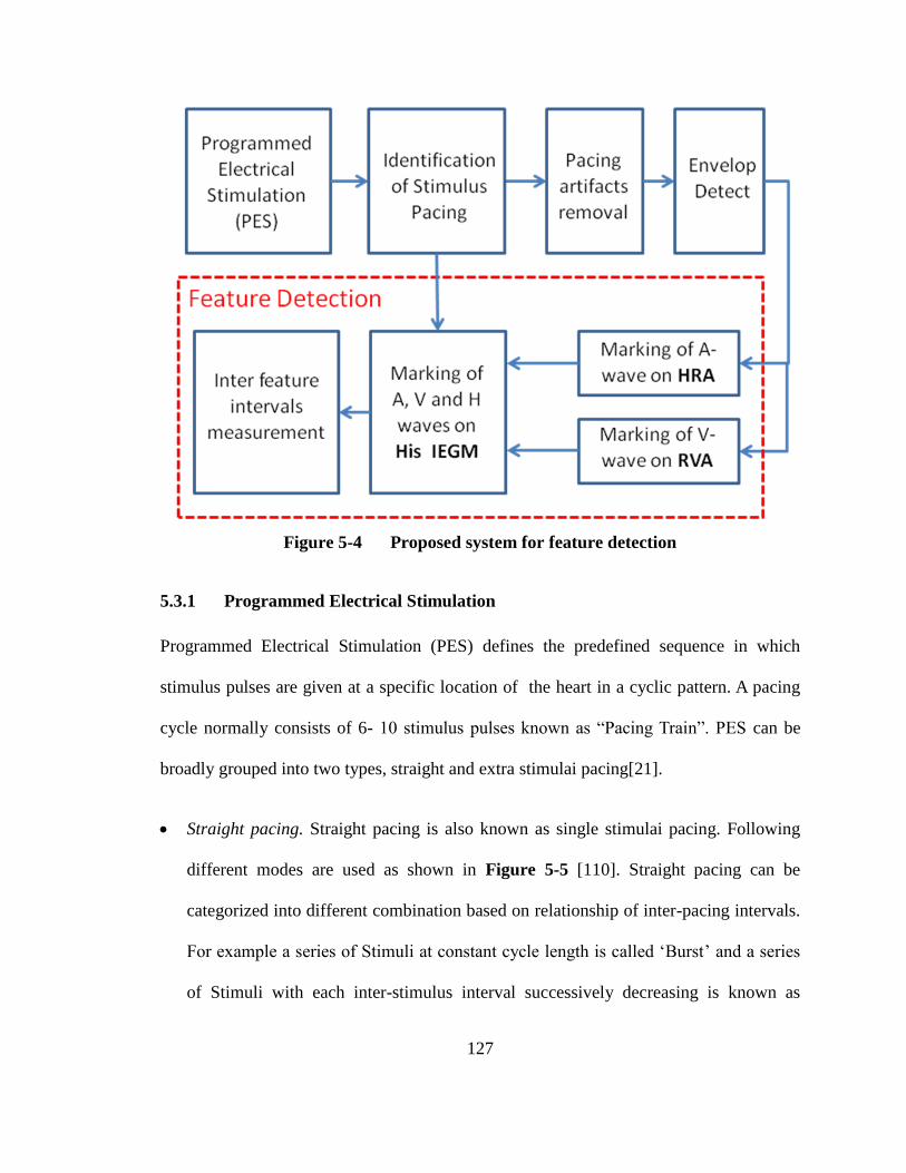
127

Figure 5-4 Proposed system for feature detection

5.3.1 Programmed Electrical Stimulation

Programmed Electrical Stimulation (PES) defines the predefined sequence in which

stimulus pulses are given at a specific location of the heart in a cyclic pattern. A pacing

cycle normally consists of 6- 10 stimulus pulses known as “Pacing Train”. PES can be

broadly grouped into two types, straight and extra stimulai pacing[21].

Straight pacing. Straight pacing is also known as single stimulai pacing. Following

different modes are used as shown in Figure 5-5 [110]. Straight pacing can be

categorized into different combination based on relationship of inter-pacing intervals.

For example a series of Stimuli at constant cycle length is called ‘Burst’ and a series

of Stimuli with each inter-stimulus interval successively decreasing is known as

128

‘Ramp’ as shown in Figure 5-5. In incremental pacing, pacing cycle length of each

Stimuli drive train is shortened by 10-50 msec from previous whereas in decremental

case it is vice versa.

Figure 5-5 Straight Pacing [110].

Extra stimuli pacing. In Extra stimuli pacing, additional pulses (extra stimuli) are

delivered at the end of a drive train [18]. It is useful especially for checking of

refractory period. Figure 5-6 shows a baseline drive of eight beats, which is delivered

at a constant cycle length (S1S1) by a stimulator. Another stimulus (S2) known as

extra stimulus is placed in succession to basic drive however, with reduced inter-

stimuli interval (S1S2); extra stimuli can be single, double or triple which are

designated as S2, S3, and S4, respectively. Generally, the extra stimuli are initiated at

80% to 90% of the drive cycle length. With the addition of each extra pulse, the

intervals are made shorter and shorter.

129

Figure 5-6 Extra Stimuli Pacing [110].

In this chapter, AVNRT and AVRT (reentrant tachycardia) have been focused to be

differentiated through time domain analysis. In reentrant tachycardia, the refractory

periods of dual/accessory pathways in AV conduction system are key factors. For

monitoring of refractory periods, the extra-stimulus (premature) pacing method can be

applied effectively [111]. For identification of AVNRT (typical) tachycardia, the most

suitable option is to apply extra-stimulus pacing through HRA catheter however, pacing

from other catheters can also be used for further confirmation of the APs location [8]. In

this study, extra-stimulus pacing is applied at HRA catheter for evaluation of AVNRT

(typical) with the PES protocol consisting of a basic drive train of eight stimuli (S1) with

pulse width of 2.0ms, followed by single extra-stimulus (S2). The protocol starts at

600/400ms (S1S1/S1S2) inter-stimuli/extra stimulus interval and S1S2 is decreased by

10ms in each subsequent pacing train.

130

5.3.2 Identification of Stimuli Pacing Train

Identification of stimuli pacing is required for four main reasons:

The timing of stimulus pulses are required to be determined,

The protocol of pacing has to be determined,

The pacing artifacts induced in other IEGM leads is required to be removed,

The location of pacing has to be verified as the reference while determining features

in other IEGMs e.g. stimuli in HRA IEGM are required to be used as reference for

identification of ‘A’ in His IEGM.

When pacing is carried out through any of catheter, the stimuli contain maximum

amplitude on a normalized IEGM and pulses can be easily identified and marked by

thresholding method. After identification of first pulse, the successive pulses are looked

within 800ms window from the preceding pulse as straight pacing always start with pulse

to pulse gap normally less than 700ms. The routine extra-stimulus pacing protocol

usually start at 600/400ms (S1S1/S1S2). The gap between first and second stimulus pulse

determines S1. When gap between two successive pulses is less than (S1S1-100ms), the

next pulse is counted as extra stimulus and gap between them is marked as S2. After

marking of 1st extra stimulus, 2

nd extra stimulus is looked within window having span of

(S1S2 - 50ms) and if found, it is marked as S3. For validation of identified stimuli pulse

train, some verification checks are performed e.g. the duration of each identified stimulus

should be less than 5ms to be counted as valid because usual stimulus pulses applied have

1-2ms pulse width (PW). Similarly, if number of detected stimuli in a pulse train is less

than six then it is taken as some artifact and are rejected to be a valid pulse train. The

algorithm for detection of pacing stimulus protocol is shown in Figure 5-7. The algorithm

131

can be extended for detection of further extra stimuli pulses, in the same way as applied

for detection of 1st and 2

nd extra stimulus pulses.

Figure 5-7 Algorithm for detection of PES protocol

132

5.3.3 Pacing Artifact Removal

In EP procedures, pacing is usually carried out through a single IEGM lead, however the

influence of this pulse is seen on other leads which, causes distortion known as pacing

artifacts [111]. Pacing artifacts are observed in all leads, therefore it is necessary to mark

the duration of stimulus and remove pacing artifacts from all leads especially, His IEGM.

For example, if pacing is done through HRA catheter, pacing pulses are marked in HRA

IEGM and pacing artifacts are eliminated successfully in His catheter by introducing a

10ms blanking interval in recorded His IEGM [98].

0 0.5 1 1.5 2

0

0.2

0.4

0.6

0.8

1

Time

Am

pli

tud

e

HisP with pacing arti fact

Pacing Artifact

Figure 5-8 HisP with pacing artifact

The detection of stimulus in HRA catheter is done with thresholding method. The pacing

artifacts are clearly visible in Figure 5-8 and in presence of these pacing artifacts, there is

likely chance of wrong detection of ‘A’ and ‘H’ waves. Therefore, the pacing artifacts are

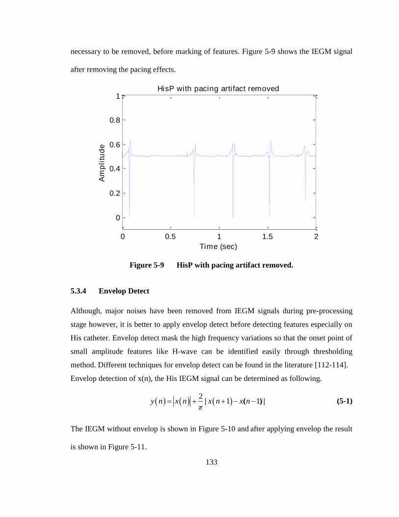
133

necessary to be removed, before marking of features. Figure 5-9 shows the IEGM signal

after removing the pacing effects.

0 0.5 1 1.5 2

0

0.2

0.4

0.6

0.8

1

Time (sec)

Am

pli

tud

e

HisP with pacing arti fact removed

Figure 5-9 HisP with pacing artifact removed.

5.3.4 Envelop Detect

Although, major noises have been removed from IEGM signals during pre-processing

stage however, it is better to apply envelop detect before detecting features especially on

His catheter. Envelop detect mask the high frequency variations so that the onset point of

small amplitude features like H-wave can be identified easily through thresholding

method. Different techniques for envelop detect can be found in the literature [112-114].

Envelop detection of x(n), the His IEGM signal can be determined as following.

2

1 1| ( ) | y n x n x n x nπ

(5-1)

The IEGM without envelop is shown in Figure 5-10 and after applying envelop the result

is shown in Figure 5-11.

134

Figure 5-10 IEGM of His catheter without envelop

Figure 5-11 IEGM of His catheter after applying envelop detect

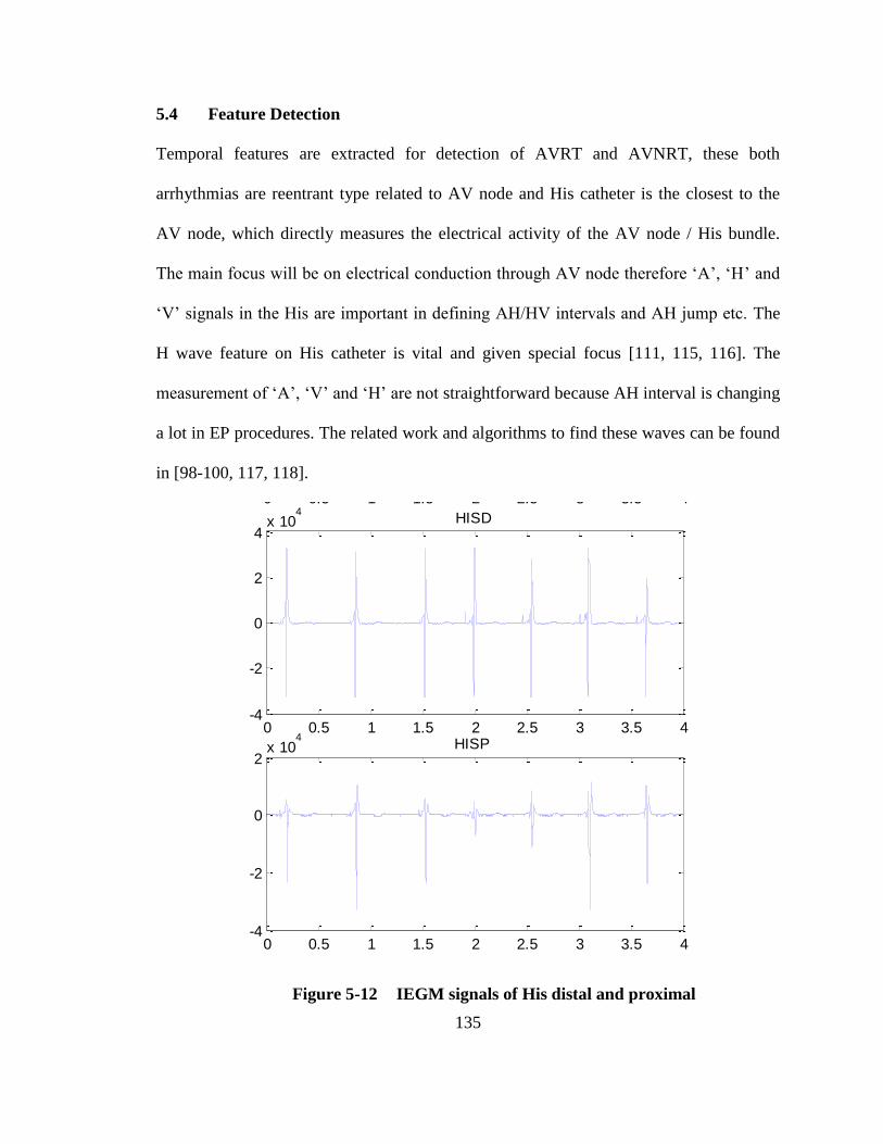
135

5.4 Feature Detection

Temporal features are extracted for detection of AVRT and AVNRT, these both

arrhythmias are reentrant type related to AV node and His catheter is the closest to the

AV node, which directly measures the electrical activity of the AV node / His bundle.

The main focus will be on electrical conduction through AV node therefore ‘A’, ‘H’ and

‘V’ signals in the His are important in defining AH/HV intervals and AH jump etc. The

H wave feature on His catheter is vital and given special focus [111, 115, 116]. The

measurement of ‘A’, ‘V’ and ‘H’ are not straightforward because AH interval is changing

a lot in EP procedures. The related work and algorithms to find these waves can be found

in [98-100, 117, 118].

0 0.5 1 1.5 2 2.5 3 3.5 4-5000

0

5000

10000lead I

0 0.5 1 1.5 2 2.5 3 3.5 4-4

-2

0

2

4x 10

4HISD

0 0.5 1 1.5 2 2.5 3 3.5 4-4

-2

0

2x 10

4HISP

Figure 5-12 IEGM signals of His distal and proximal

136

Figure 5-12, shows the real His_P and His_D IEGM signals. It is evident that HisP and

HisD show clear ‘V’ wave while ‘A’ and ‘H’ are not clearly visible in their waveform at

this scaling because ‘A’ and ‘H’ have very low threshold as compared to ‘V’. For

marking of A, V and H wave on His catheter, first we have to mark the A wave on HRA

catheter and V wave on RVA catheter.

0 0.5 1 1.5 2 2.5 3-0.5

-0.4

-0.3

-0.2

-0.1

0

0.1

0.2

0.3

0.4

0.5

RVA

Time (sec)

No

rmali

zed

Am

pli

tud

e

RVA-D

V-wave

Figure 5-13 Onset of VRVA

5.4.1 “V” on RVA Catheter

Since the amplitude of VRVA (V wave on RVA catheter) is much larger than the actual

baseline, the onset of V wave is easiest to find as following.

137

Peak detection of VRVA. The peak of the V wave is marked on a normalized RVA

IEGM by empirically defined threshold, which is generally selected as 1/3 of

maximum value of RVA IEGM (VRVA-max) [111].

Marking onset of VRVA. The VRVA-on (onset of the VRVA) is searched within a 30ms

window prior to VRVA-max, such that onset is marked when VRVA crosses a threshold of

1/15 of VRVA-max [100, 111, 119]. The results are shown in Figure 5-13.

0 0.5 1 1.5 2 2.5 3 3.5 4-0.5

0

0.5HRA

Time (sec)

No

rmali

zed

Am

pli

tud

e

HRA-P

A(onset)

Figure 5-14 Onset of AHRA

5.4.2 “A” on HRA Catheter

Similarly, AHRA (A wave on HRA) and stimulus pulses dominates the HRA IEGM and

can be marked through thresholding technique as following.

138

Peak detection of AHRA. The AHRA-max (peak of A wave) is located on a normalized

HRA IEGM with reference to threshold level defined as 1/3 of maximum value of

HRA IEGM [111].

Marking onset of AHRA. The AHRA-on (onset of the AHRA) is searched prior to AHRA

within a 30ms window prior from the peak with reference to a threshold of 1/15 of

AHRA-max [100, 111, 119]. The results are shown in Figure 5-14.

5.4.3 “A”, “V” and “H” on His Catheter

Next, locate the onset of characteristic waves on the His catheter. The crucial step is the

measurement of ‘A’, ‘V’ and ‘H’ from the His channel which contains varying in time

pulses in consecutive heart beats and sometimes the thresholds of pulses are very low and

sometimes the pulses are even mixed into each other. His catheter recording contains the

AHis (A wave on His), HHis (H wave on His) and VHis (V wave on His) [120]. In His

channel, it is understood that in between every VV interval two important pulses are

present during a normal conduction system, one is ‘H’ and other is ‘A’. Out of A, H and

V waves, V wave has normally highest amplitude and H wave is smallest feature just

before the onset of V wave. Therefore it is preferred option to first detect ‘V’ on His

IEGM followed by ‘A’ and ‘H’ in sequence under certain criteria.

Once the ‘A’ pulse is detected, the only left item is the ‘H’ wave, which is present

between ‘A’ and ‘V’ waves. The identification of ‘H’ wave is most difficult especially in

presence of noise therefore some extra measures have to be taken for foolproof detection

of ‘H’ wave onset point. For a valid ‘H’ wave, the His catheter must be appropriately

139

placed and IEGM signal should be acquired such that it contains minimum noise.

Following features are marked on preprocessed (including envelop detection) His IEGM.

0 0.5 1 1.5 2-0.5

0

0.5

1RVA

Time (sec)

No

rmali

zed

Am

pli

tud

e

RVA-D

V-wave

0 0.5 1 1.5 2-0.5

0

0.5

1HISD

His-D

V-onset

V-offset

Figure 5-15 Earmarking of VHis-on and VHis-off

Marking VHis. ‘V’ appears first in RVA IEGM and then reflected in HRA IEGM,

therefore, VHis-max (the peak of V-wave on the His catheter) is searched within a

100ms window after VRVA-on [111]. The VHis-on (the onset of the VHis) is searched

within a 30ms window prior from its peak and is marked when VHis crosses a

threshold of 1/15 of VHis-max and the offset of the VHis (VHis-off) is searched after VHis-

140

max, when VHis crosses a threshold of 1/12 of VHis-max [111, 119]. Result is shown in

Figure 5-15.

Marking AHis. After marking of VHis-on, AHis-max (the peak of ‘A’ on the His catheter) is

marked as highest peak within a window starting 40ms after S2 (or AHRA-max) to 40ms

before VHis-on and AHis-on (the onset of the AHis) is marked prior to AHis when it crosses

a threshold of 1/12 of AHis-max [111]. Similarly, AHis-off (the offset of the AHis) is

marked after AHis-max, when AHis crosses a threshold of 1/12 of AHis-max [111].

2.55 2.6 2.65 2.7 2.75 2.8 2.85 2.9

-0.4

-0.3

-0.2

-0.1

0

0.1

0.2

0.3

0.4

HISD

Time (sec)

No

rmali

zed

Am

pli

tud

e

HisD

V-on

V-off

H-on

Figure 5-16 Marking of HHis-on on His IEGM

Marking HHis. Detection of H wave is the most difficult and requires higher-level

precautions to avoid any false detection. The onset of H (HHis-on) is searched in the

window between the AHis-off and VHis-on [100]. First, peak of ‘H’ (HHis-max) is searched

in the window having span from (AHis-off + 50ms) to (VHis-on - 30ms) and HHis-on is

141

marked prior to HHis-max when it crosses a threshold of 1/12 of HHis-max [111]. The

marking of HHis-on is shown in Figure 5-16.

5.4.4 Validation of HHis-on

Since HHis is a small amplitude feature and normal ‘H’ wave is 10-25ms wide [120].

Validation of HHis-on is required to minimize the possibility of false detection. Following

checks are performed for validation of HHis-on.

HV interval. The first check disregards any H wave onset detected too near or too far

from the His on

V

location. HV interval ranges from 35-55ms therefore HHis-on which

correspond to an HV interval outside the range 35–55msec are rejected [27, 120].

Variance of His IEGM. The second check is associated with the variance of the

signal. Here the main idea is same as that used by doctors, i.e. if the recording is too

noisy then proper decisions cannot be made based on that; so that particular recording

is discarded and a new recording has to be acquired. Likewise, we say that if the

signal contains too much noise, then it is very likely that the detected onset point of

the H wave is faulty.

To incorporate this theme into our algorithm, HIS IEGM within the local search

window is divided into n parts. It is assumed that the HHis-on lies in the nth part of this

window and variance of this part is greater than other n-1 parts. If variance of the

region not containing HHis-on is found to be higher than the region detected to contain

HHis-on, then there is possibility of wrong detection. Therefore detection of HHis-on is

rejected for this activation. Feature detection algorithm is summarized in Figure 5-17.

142

Figure 5-17 Feature detection algorithm

143

5.5 Results

Table 5-1 shows the results of the feature detection algorithm. The algorithm developed

was tested against database of 20 patients collected from EP lab of AFIC/NIHD Pakistan.

The data contained more than 4500 useful activations. The percentage accuracy of V, A

and H waves found to be 95.06%, 89.93% and 98.33% respectively.

Table 5-1 Result of Feature Detection Algorithm

Feature

Points

Total

Activations

Correct

Detections

Wrong

Detections

Missed

Detections

Accuracy

(%)

A Wave 1230 1202 0 28 97.72

H Wave 1192 1148 8 36 96.31

V Wave 2156 2149 0 7 99.63

4578 4499 8 71 98.27

5.6 Summary

For automated arrhythmia detection during an EP study, the most important aspect is

accurate marking of ‘A’, ‘V’ and ‘H’ features on different IEGMs. These features have

different widths and amplitudes on different catheters. For accuracy of inter feature time

intervals, the selection onset of features is the best criteria. Moreover, the ‘H’ feature is

most sensitive to be identified because of its minute amplitude. In this chapter, the

method for marking of onset points of all features has been defined and to ensure

validation of ‘H’ feature, special checks are introduced to prevent false detection.

144

CHAPTER 6

IDENTIFICATION OF REENTRANT TACHYCARDIA

In this chapter, reentrant tachycardia, which include AVRT and AVNRT, are

analyzed using IEGM signals in time domain. For analyzing reentrant

tachycardia, extra stimuli pacing of heart is done under a specific protocol and

heart is enforced to enter in tachycardia state. The foremost requirement is the

IEGM feature detection and then determine the time gaps between different

features. Based on the outcomes of the induced tachycardia, the type of

arrhythmia can be verified. The feature detection has been covered in previous

chapter and those features and their time intervals are analyzed to differentiate

AVNRT and AVRT arrhythmia. The sequence of this chapter is as follow, first of

all different steps involved for EP evaluation are discussed, key features detection

method defined, proposed algorithms for classification of AVRT/AVNRT are

presented and then results of proposed method are discussed.


Automated arrhythmia detection algorithms have been developed extensively for surface

electrocardiograms (ECG) [121, 122]. The existing literature also includes algorithms

based on IEGMs developed for usage in Implantable Cardioverter Defibrillators (ICD)

[123]. However, programming routines specifically meant for clinical EPS are very

limited.

Among several types of tachycardia and bradycardia, the most common arrhythmia faced

by electrophysiologist is AVNRT. It is a type of reentry tachycardia which occurs due to

145

problem in Atrio-ventricular (AV) node in which 2 pathways exist instead of normal

single fast pathway which creates a loop and initiates tachycardia [15, 27]. The AVNRT

has conventionally divided into two types named as typical AVNRT (slow-fast) and

atypical AVNRT (fast slow) however majority cases (80-90%) belongs to typical

AVNRT and that’s why typical AVNRT has been focused in this work [124-126]. For

differentiation of AVNRT, no unanimously accepted method has been adopted [124].

Electrophysiologists apply various protocols for identification of AVNRT during an EP

study [127-129]. For AVNRT, one of criteria most commonly used is to observe AH

jump [126-128].

AVRT is considered as second most common type of reentrant tachycardia [23]. The

AVRT are of two types named as Orthodromic (typical) AVRT and Antidromic

(atypical) AVRT. Differentiation maneuvers between orthodromic and antidromic AVRT

have been defined well by K. Tanka et. al [130]. For initiation and persistence of AVRT,

the presence of APs between atria and ventricle is a compulsory criteria [131]. During

AVRT, the atria and ventricles contract sequentially and the parameters used to

distinguish AVRT from other tachycardias can be found in [18, 20, 27]. For AVRT case,

one criteria is that the A-V interval must be greater than V-A interval and second criteria

is that V-A interval must be greater than 35-65ms for a diagnosis in favour of AVRT [20,

118].

6.2 Dataset

20xPatient’s dataset has been collected from AFIC/NIHD Pakistan and MIT Physionet

database [12]. AFIC/NIHD dataset includes the verified cases of both AVRT and

AVNRT. The dataset contains IEGMs recorded from 2-5-2 mm quadripolar HRA, RVA

146

& His catheters and 2-5-2 mm decapolar CS catheter. For identification of AVRT and

AVNRT, primarily the data from HRA, RVA and His IEGMs are used; however, the CS

IEGM can be used in secondary stage to confirm the location of APs. The recorded

IEGMs are in the range of -5mV to +5mV, which are digitized at sampling rate of 2K

with 16 bit precision.

6.3 Methodology

Proposed methodology comprises multiple stages as shown in Figure 6-1 to detect

AVNRT/AVRT arrhythmia from pre-processed IEGM signal during EP study. The

description of these steps is as following.

Figure 6-1 Proposed methodology for detection of AVNRT/AVRT

147

6.3.1 Extra Stimuli Pacing

For identification of typical AVNRT, the extra-stimulai pacing in anti-grade mode at

HRA catheter have been used and ‘A’, ‘H’ and ‘V’ are marked on His IEGM as shown in

Figure 6-2. The pacing protocol starts with an S1S1 interval of 600ms and an S1S2 (extra

stimulus gap) is at least 60ms higher than the documented wenckebach interval. It is very

common to start at 600/400ms (S1S1/S1S2). If the patient heart rate is above 100bpm

(100bpm = 600ms), you will need to start at a faster cycle length for S1. Once stimulation

has begun, the S1S2 interval is gradually decreased by 10-20ms for each new pacing

train. The process is continued until the presence of AVNRT tachycardia is either verified

or ruled out.

Figure 6-2 Extra stimulus pacing at HRA and marking of A, H and V waves on

His catheter [120].

6.3.2 Atrial/Ventricle Activation Rate/Regularity

Depolarization/activation rate of both atria and ventricle is important to decide the type of

arrhythmia. Moreover, it is also important to observe that activation rate of both atria and

ventricle is same or different. For example, in AVNRT/AVRT, the A:V conduction is

148

usually 1:1 and in case of variations, the possibility of AVNRT/AVRT is declined.

Regularity of tachycardia is required to be checked. As in ECG signal, the R-R interval

determines beat-to-beat regularity, similarly in IEGM, the A-A interval extracted from

HRA and the V-V interval extracted from the RVA can be used to confirm regularity of

the rhythm.

6.3.3 Inter Feature Time Duration

The time intervals between A, V and H fudicial points are important features to be used

for detection of many arrhythmias as shown in Figure 6-3. AH interval measurement on

His catheter provides time gap between atrial wave appeared at inter-atrial tissues to first

depolarization at His bundle. The AH interval (equivalent to PR interval observed on

ECG) defines the propagation delay occurred at AV node and normal range of AH

interval is 60-125ms [120]. HV interval gives us the time gap of passing wave front from

bundle of His to Purkinje fibers. AH intervals (AHis-on to HHis-on) and HV intervals (HHis-on

to VHis-on) are measured and count as a feature for decision of arrhythmia classification.

AA or A1-A2 interval (time gap between AHis-on of 1st activation to AHis-on of 2

nd

activation) and HH or H1-H2 interval (time gap between HHis-on of 1st activation to HHis-on

of 2nd

activation) also counts as features.

6.3.4 Special Characteristic Verification

Once the electrophysiologist identify an arrhythmia then some special characteristic

related to that arrhythmia is verified/located. For AVNRT, AH interval provide us

information of AH jump. AA and VV interval tell us about atrial and ventricle rate

regularity as well as AV block. Also for the case of AVNRT, the measurement of VA

149

interval and AH/HA ratio facilitates us to differentiated between typical and atypical

AVNRT. For AVRT case, one criteria is that the A-V interval must be greater than V-A

interval [20, 118]. For the case of AVRT, the location of APs can also be verified with

the help of timings sequence in different IEGMs.

Figure 6-3 Importance/correlation of electric activity in different electrodes [18].

150

Figure 6-4 Interval measurements [18].

6.4 Identification of AVNRT

In AVNRT, two pathways exist in or around AV node, out of which one is faster as

compared to other. Typical AVNRT is characterized by regular rhythm, 1:1 atrial to

ventricle activation ratio and narrow QRS (QRS < 120ms) in ECG [125, 132, 133]. In

typical AVNRT, VA interval is lesser than 60ms and vice versa for atypical AVNRT

[134, 135]. AH/HA ratio of a typical AVNRT must be greater than unity [124]. AH jump

151

is the key feature which is used to classify AVNRT [136]. AH interval is the time

difference between AHis(On) and H His(On) and is measured for all the beats on His IEGM.

AH jump is basically an increase of time measurement between two successive AH

intervals when HRA catheter is stimulated with extra-stimulus technique in which each

time S1S2 interval is reduced gradually by 10–20ms. The effect of extra stimulus pulse

reflects on the ‘H’ wave in same proportion. There comes a stage when the AH interval

does not appear to be in proportion to extra stimulus rather it becomes significantly larger

than its previous one indicating the AH jump because of the reason that fast pathway has

become refractory and pulse is being passed though slow path as shown in Figure 6-5.

Figure 6-5 Slow-fast AVNRT and observation during EP study [125].

152

(a)

(b)

http://www.theeplab.com/B-The-Members-Center/F000-Cardiac-Arrhythmias/G-AVNRT/FG00-AVNRT.php

Figure 6-6 Presence of AH jump with extra stimulus pacing protocol change over

from (a) 600/300ms to (b) 600/290ms.

http://www.theeplab.com/B-The-Members-Center/F000-Cardiac-Arrhythmias/G-AVNRT/FG00-AVNRT.php

153

The AH interval is counted as valid AH jump if AH interval is increased by 50ms or

more with a 10ms (or 20ms) decrement in S1S2 interval. Figure 6-6 demonstrate the AH

jump, an extra stimulus pacing 600/300 is applied in Figure 6-6(a) which gives 146ms

AH interval. However in the next series of pacing when S1S2 has been decreased by

10ms i.e. with 600/290ms extra stimulus pacing protocol, we notice that AH interval

becomes 211ms which means 65ms (211-146) AH jump is achieved and AVNRT is

verified.

2.2 2.4 2.6 2.8 3 3.2 3.4

0.2

0.4

0.6

0.8

1

Time (sec)

Am

pli

tud

e

His with A, V and H measured

His

H

A

AH Jump

Figure 6-7 AH jump is clearly visible at third instance of the figure. In first two

instances, the AH interval is normal whereas at 3rd

instance AH interval is large

AH jump is clearly visible in simulation result as shown in Figure 6-7. The AH intervals

are drawn separately in Figure 6-8. This figure shows the presence of the AH jump at

instance #38. A simple classifier is used to check if AH jump is greater than 50ms or not.

154

33 34 35 36 37 38 390

100

200

AH

in

terv

al

(ms)

AH Interval Measurement

33 34 35 36 37 38 39-100

-50

0

50

100

150

Instance Number

A2H

2 -

A1H

1 (

ms)

AH Jump

AH Jump

Figure 6-8 AH Interval and AH Jump measurement

6.5 Identification of AVRT

In AVRT, an APs exists between atria and ventricle in addition to AV node. The

direction of electric pulse through APs can be antidromic (atypical) or orthodromic

(typical) based on which AVRT are further categorized as shown in Figure 6-9. Typical

AVRT is most common between two types. AVRT is usually verified through

constant/decremental retrograde pacing through RVA catheter and Antegrade pacing at

HRA catheter as shown in Figure 6-9 [137-139]. Typical AVRT is characterized by

regular rhythm, 1:1 atrial to ventricle activation ratio and narrow QRS (VA/AV < 1) in

ECG [132, 133]. Some additional criteria define that the VA interval in case of typical

AVRT should be greater than 60ms but must be lesser than AV interval [124, 126]. The

location of APs can be determined by monitoring the earliest reentrant activation

155

appearance at different locations of catheter. For the case of AVRT, following three

criteria can be defined

Right sided APs. If the earliest reentrant activation appears in the HRA catheter

Left sided APs. If the earliest reentrant activation appears in the CS catheter.

Septal (center) APs. If the earliest reentrant activation appears in the His catheter

(a) (b)

(c)

Figure 6-9 (a) Orthodromic AVRT (b) Antidromic AVRT (c) Antegrade versus

retrograde pacing for AVRT verification [137].

156

Figure 6-10 Reentrant arrhythmia detection algorithm

6.6 Classification Algorithm between AVRT and AVNRT

The proposed algorithm uses the basic features 'V’, ‘A’ and ‘H’ waves and determines

AVRT and AVNRT specific features i.e. AH jump, A-V interval and V-A intervals etc.

AH jump is the key feature to classify AVNRT and AV & VA intervals are key features

related AVRT. The structure of the algorithm is shown in Figure 6-10. Table 6-1 shows

the result of arrhythmia detection.

157

Table 6-1 Result of Arrhythmia Detection

Dataset of

Verified

Arrhythmia

Arrhythmia AVRT AVNRT

NSR & Misc

SVT

(except AV

node

reentrant)

Total events

No of Events 436 559 1133 2128

Arrhythmia

Detection

Result

AVRT 408 4 4 416

AVNRT 7 542 3 552

NSR & Misc

SVT

(except

reentrant)

9 5 1121 1135

Discarded

Events

12 8 5 25

The confusion matrix is defined as under to determine sensitivity, specificity, positive

prediction value (PPV) and negative prediction value (NPV) of an arrhythmia [140].

Gold-standard

arrhythmia present

Gold-standard

arrhythmia absent

Detection

positive True Positive (TP) False Positive (FP)

TP

TP FPPPV

Detection

negative False Negative (FN) True Negative (TN)

TN

TN FNNPV

TP

TP FNSensitivity

TN

TN FPSpecificity

Confusion matrices and determined sensitivity, specificity and PPV against AVRT and

AVNRT are as under.

158

AVRT AVRT arrhythmia Non-AVRT arrhythmia

AVRT

detected 408 8

PPV=

98.08%

AVRT not

detected 28 1684

NPV=

98.36%

Sensitivity=

93.58%

Specificity=

99.53%

AVNRT AVNRT arrhythmia Non-AVNRT

arrhythmia

AVNRT

detected 542 10

PPV=

98.19%

AVNRT not

detected 17 1157

NPV=

98.55%

Sensitivity=

96.96%

Specificity=

99.14%

Table 6-2 shows the accuracy of the proposed system in term of sensitivity, specificity

and PPV and NPV.

Table 6-2 Sensitivity, Specificity, PPV and NPV Results

Cardiac

arrhythmia

Sensitivity (%) Specificity (%) PPV (%) NPV (%)

AVRT 93.58 99.53 98.08 98.36

AVNRT 96.96 99.14 98.19 98.55

159

The results show that performance of the proposed algorithm for arrhythmia detection in

clinical EPS is comparable to manual diagnostic procedures.

6.7 Summary

Real patient data having AVNRT and AVRT events have been acquired from

AFIC/NIHD and events are verified by cardiologist to be used as gold standard for

checking accuracy of proposed work. An algorithm is presented for detection of AVNRT

and AVRT using IEGM features during an EP study. The proposed algorithm performs

well and gives sensitivity 96.96% for AVNRT and 93.58% for AVRT. The specificity

remained 99.14% for AVNRT and 99.53% for AVRT. The main significance to develop

this system is to reduce the time required by electrophysiologist for manual calculations

to find the different features and their time intervals for detection of AVNRT and AVRT

arrhythmias.

160

CHAPTER 7

FREQUENCY DOMAIN ANALYSIS FOR IDENTIFICATION OF

ATRIAL TACHYCARDIAS

Cardiac Electrophysiology (EP) encompasses study of the IEGM to analyze

different types of arrhythmias. Arrhythmias are investigated by pacing the heart

under a specific protocol and studying the response in return. The IEGM are

studied by the Electro physiologist visually (using the monitor screens), which is

time consuming and highly dependent on individual expertise. However, it has

also been observed that during an EP stimulation process, a patient may develop

Atrial Fibrillation (AF). In order to proceed further with the diagnosis /automated

detection of an arrhythmia, the patient has to be taken out of AF. Although

Electro physiologist, based on their expertise can identify AF by visual

monitoring of atrial IEGM, a need was felt for real time automated detection of

AF as well as its differentiation from AFL, AT and NSR.

To fulfill the requirement, a system (algorithm) is required to be designed with

consideration of following basic decisions.

The selection of time/statistical/frequency domain for the desired system.

The base of differentiation among NSR, AT, AFL and AF

Pre-processing requirement for extraction of atrial activity.

Suitable Location of IEGM catheter for monitoring of AF activity.

Baseline frequency range selection of atrial activations of NSR, AT, AFL and

AF.

161

PSD estimation response against activations of NSR, AT, AFL and AF.

Suitability of conventional PSD features (DF, RI, etc) for desired task.

Considering all above design parameters, frequency domain has been selected for

differentiation of atrial IEGMs in this work. Dominant frequency (DF) is estimated

using Welch method to find out atrial activation rate during NSR, AT, AFL and AF. A

new spectral parameter, Average Power Spectral Ratio (APSR), has been identified

for ensuring reliability of DF for AF detection as well as differentiation of AF from

other atrial arrhythmias. The proposed algorithm successfully detects and

differentiates between NSR, AT, AFL and AF with an accuracy of 99.53 %..


The atrial rate can be used for detection of AF as well as its differentiation from other

arrhythmias. Atrial rate for NSR normally ranges from 60- 100 bpm (beat per minute).

For AT, atrial rate has the range from 100- 240 bpm, however, in AFL the heart beats

goes up to 300 bpm [34]. During AF, the atrial rate can go beyond 300 bpms [36]. Atrial

rate calculation in time domain for NSR, AT, and AFL, being regular and periodic

signals is quite simple. However automated detection of AF, being an irregular signal

involves application of frequency/ time frequency/ statistical domain techniques [141-

151].

Using spectral estimation technique, Jason Ng et al and Rakesh et al have explained the

concept of DF to estimate the atrial activation rate [152, 153]. The DF is defined as the

frequency containing maximum power in frequency domain; Vassil et al. has indicated

that “it can be easily applied to estimate the local atrial activation rate in AF” [154]. This

162

concept has been employed in this section to find atrial activation rate for detection and

differentiation between NSR, AT, AFL and AF.

For periodic activations, like NSR, AT, and AFL, DF gives the robust estimation of

activation rate however, for irregular activation like AF, the estimation may not be as

robust. Therefore, DF analysis for AF is built upon selection of the lowest-noise signal.

An index, known as Regularity index (RI), has been frequently used to ensure the

reliability of DF [155-160]. Mostly, DF with RI > 0.2 has been considered reliable for AF

detection and its further analysis [157-160]. Millet J et al. used a set of 8 x spectral

parameters for differentiation of NSR, AFL and AF [150]. Later, Rieta J. et al. shortlisted

the set of parameters from 8 to 5 [161].

Based on atrial activation rate, DF ranges for NSR and regular atrial arrhythmias can be

well defined i.e. 1~1.7 Hz for NSR, 1.7~4 Hz for AT and 4~7 Hz for AFL. However for

AF, different researchers have come up with different DF ranges and the most accepted

range has been identified as 3~12 Hz [147, 150, 158-160, 162]. On closer examination of

these DF ranges, it can be observed that DF range of AF overlaps with AT in DF range of

3~4 Hz and with AFL in DF range of 4~7 Hz. These overlapping frequency ranges

restrict DF to be used as a single parameter for differentiation among AT, AFL and AF.

In this chapter, an algorithm has been proposed for detection of AF and its

differentiation from NSR, AT and AFL during an EP study using DF. For reliability of

DF, the RI parameter is used conventionally. As for as reliability of DF is concerned, RI

parameter works good but does not assist to differentiate AF from AT and AFL in their

overlapping frequency ranges therefore, we need another parameter for differentiation. A

new spectral parameter named as “Average Power Spectral Ratio” (APSR) has been

163

introduced which differentiates among AT, AFL and AF in their overlapping ranges as

well as determines the reliability of DF. This new parameter is less complex to be

calculated and provides more robust result as compared to RI thus eliminates the

requirement of RI for determining the reliability of DF.

Table 7-1 ECG and IEGM Data – AFIC/NIHD

CHANNEL NO LABEL DESCRIPTION

1 I ECG

2

3

4

5

6

7

8

9

10

11

12

aVF

V1

HRAD

HisD

HisP

CS 9-10

CS 7-8

CS 5-6

CS 3-4

CS 1-2

RVAD

“

“

HRA distal

His distal

His proximal

CS catheter

“

“

“

“

RV distal

7.2 Dataset

The majority of Patient’s dataset has been collected from AFIC/NIHD Pakistan and few

from MIT Physionet database as available [12]. AFIC/NIHD dataset includes the verified

164

episodes of NSR, AT, AFL and AF recorded from HRA of 20 patients. To avoid far field

ventricular activity, IEGMs are obtained through 2-5-2 mm catheters employing

electrode pairs in bipolar configuration as shown in Table 7-1. The recorded IEGMs are

in the range of -5mV to +5mV, which are digitized at 2000 Hz sampling rate with 16 bit

precision.

MIT Physionet dataset contains the IEGMs of 8 x patients for cases of AF and AFL. The

MIT dataset was recorded in bipolar configuration from different positions of the right

atrium using 2-5-2 mm catheters sampled at 1000 samples/sec. The MIT dataset consist

of 3 x ECG leads and 5 x IEGMs bipolar signals as depicted in Table 7-2. For this study,

the electrode pair (CS 1-2) which is placed close to the annulus of SVC, has been

selected. Although this configuration is not a standard EP setup, however the selected

electrode pair (CS 1-2) provides localized atrial activity in lieu of HRA catheter.

Table 7-2 ECG and IEGM Data – MIT Physiobank

CHANNEL NO LABEL DESCRIPTION

1 II ECG

2

3

4

5

6

7

8

V1

aVF

CS 1-2

CS 3-4

CS 5-6

CS 7-8

CS 9-10

“

“

CS catheter

“

“

“

“

165

The dataset used for the proposed algorithm consist of 4000 events of verified NSR, AT,

AFL and AF cases as shown in Table 7-3.

Table 7-3 IEGM Dataset (Verified Rhythms)

Atrial Rhythm Number of events

NSR 550

AT 700

AFL 350

AF 1400

Total 4000

7.3 Methodology

In this work, atrial IEGMs from High Right Atrium (HRA) and Superior Vena Cava

(SVC) have been used for differentiation of different SVT. In order to avoid far field

ventricular activity, IEGM are recorded using catheters with minimum inter electrode

spacing (IES) in bipolar configuration [163]. Pre-processing steps as suggested by

Botteron and Jason are applied to IEGM [164, 165]. Welch method is implemented on

pre-processed IEGM for PSD estimation as highlighted by Shafa-at [166, 167]. Spectral

parameters including DF, RI and APSR have been calculated from estimated PSD.

Patterns of DF in estimated PSD of NSR, AT, AFL and AF have been analyzed. APSR

and RI have been compared for regular and irregular arrhythmias. Lastly, an algorithm

has been evolved using DF and APSR parameters to differentiate between NSR, AT,

AFL and AF.

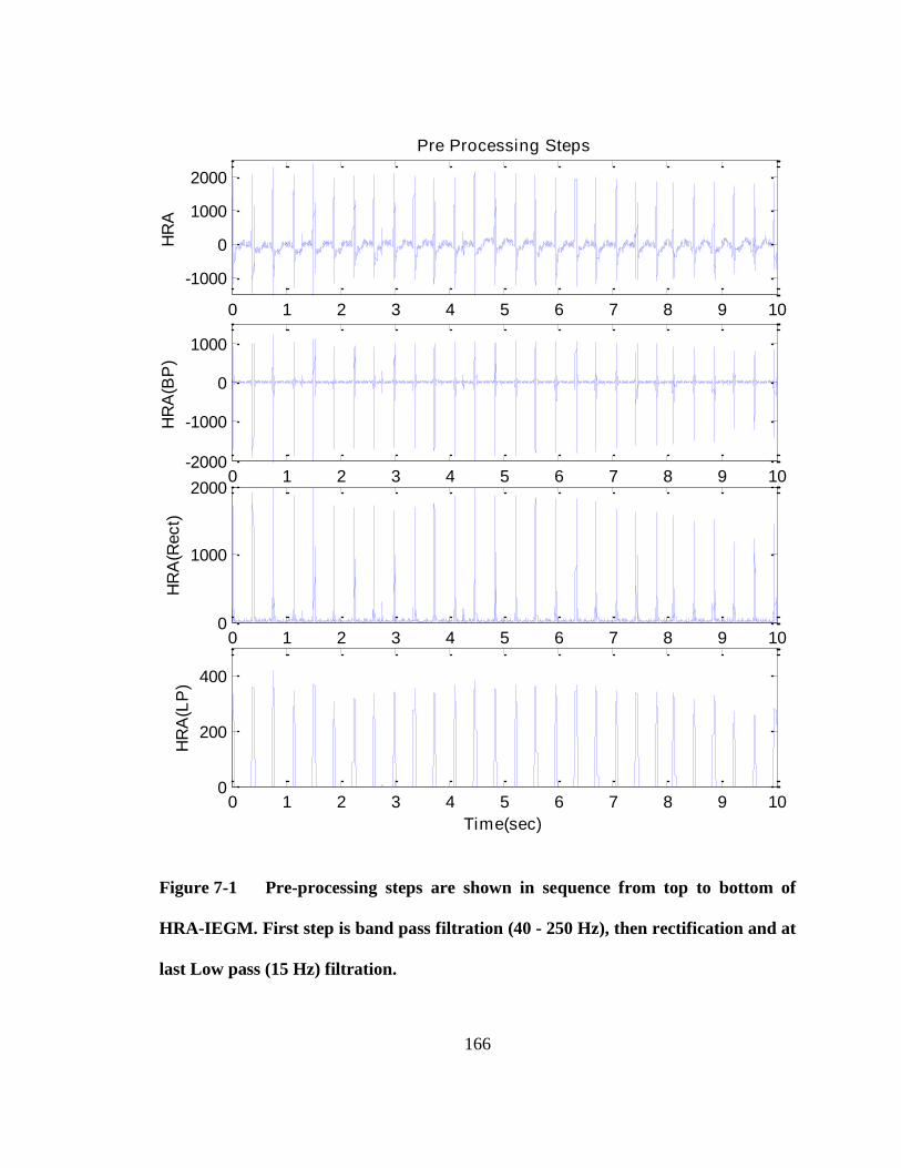
166

0 1 2 3 4 5 6 7 8 9 10

-1000

0

1000

2000H

RA

Pre Processing Steps

0 1 2 3 4 5 6 7 8 9 10-2000

-1000

0

1000

HR

A(B

P)

0 1 2 3 4 5 6 7 8 9 100

1000

2000

HR

A(R

ect)

0 1 2 3 4 5 6 7 8 9 100

200

400

HR

A(L

P)

Time(sec)

Figure 7-1 Pre-processing steps are shown in sequence from top to bottom of

HRA-IEGM. First step is band pass filtration (40 - 250 Hz), then rectification and at

last Low pass (15 Hz) filtration.

167

7.4 IEGM Pre- Processing

Pre-processing of IEGMs is carried out to obtain the signal corresponding to the local

depolarization and to restrict the frequency spectrum to physiological range [164, 168].

These include:

Band pass (40 - 250 Hz) filtering using 3rd order Butterworth filter,

Obtaining monophasic waveform by rectification and

Low pass filtering (15 Hz) using 3rd order Butterworth filter [167].

Pre-processing steps of an IEGM signal acquired from HRA catheter are shown step by

step in Figure 7-1.

7.5 PSD Estimation

For PSD estimation, a number of PSD estimation techniques have been applied in

literature; out of which Bartlett, Welch and Circular Welch method has been applied to

pre-processed IEGM for PSD estimation [166, 169, 170]. A comparison of these methods

has been performed and attached as Annexure ‘A’. Iit has been observed that Welch

method is found most suitable on the basis of the results accuracy.

In the Welch method, the signal segment is divided into P sub segments, with each sub

segment having length L. The sub segments are overlapped and modified periodograms

are computed from the overlapped P sub segments. Also, the periodogram are normalized

by the factor N to compensate for the loss of signal energy owing to the windowing

procedure [171]. Mathematically, it is calculated as

1

0

21

0

)()(1

)(ˆP

i

jnL

n

j

B eiCnxnhPLN

eP (7-1)

168

where P is no of sub segments, L is length of each sub segment, C is the overlap

between two consecutive sub segments, h(n) is windowing function and N is given by

L-1

2

n=0

1N = h(n)

L (7-2)

Length of the signal segment and sub segments has to be kept long enough to provide

the requisite frequency information however frequency resolution should be sufficiently

maintained while averaging the DFs [172]. With the experimentation, the optimum

results have been obtained for signal segment of 10 seconds duration which is divided

into nine sub segments of 2 seconds duration such that each sub segment have 50%

overlap with its consecutive sub segment.

Figure 7-2 Signal segment and Sub Segment for Estimation of PSD through

Welch method.

Modified periodogram of each sub segment with Hanning window, is taken. The average

of these nine spectral estimates gives Welch spectral estimate. Frequency resolution of

PSD is kept to be 0.1221 Hz. For real time monitoring, the signal segment is updated

169

after each second such that one new sub segment is included and one oldest sub segment

is excluded, keeping the same proportion of segment/sub segments. Figure 7-2 depicts the

signal segment and sub segments for estimation of PSD using Welch method.

7.6 Extraction of Spectral Parameters from PSD

7.6.1 Dominant Frequency

DF is referred as the frequency containing maximum PSD in frequency domain and it is

used to estimate of the local atrial activation rate [154, 173]. Usual atrial activation rate

of NSR remains within 60~100 bpm, AT within 100~240 bpm and AFL within 240~420

bpm [13, 20-23, 29-31, 33, 34]. Having estimation of PSD, the DF is determined as the

frequency having highest peak in estimated PSD in 1~12 Hz [152, 153]. For AF, the DF

range is considered 3~12 Hz. Following DF ranges are taken as the baseline of proposed

work, which also commensurate with bpm as indicated above.

NSR - 1~1.7 Hz

AT - 1.7~ 4 Hz

AFL - 4~7 Hz

AF - 3~12 Hz

It is important to note that DF range of AF overlaps with the DF ranges of AFL and AT,

therefore DF parameter alone cannot differentiate between AT, AFL and AF in their

overlapping ranges.

170

7.6.2 Regularity Index

In previous literature, RI parameter is used to establish the reliability of DF. In this work,

RI is calculated only for comparison with APSR. RI is calculated as the ratio of PSD area

under DF/harmonics (1 Hz base) to total PSD area between 1~12Hz as depicted in Figure

7-3[152]. RI is computed numerically using Simpson 3/8 and Trapezoidal rule [167].

Figure 7-3 Calculation of RI for reliability of DF

171

1 2 3 4 5 6 7 8 9 10 11 120

2

4

6

8

10

12

14

15x 10

9

Frequency (Hz)

PS

D

(a)

1 2 3 4 5 6 7 8 9 10 11 120

2

4

6

8

10

12

14

15x 10

8

Frequency (Hz)

PS

D

(b)

Figure 7-4 PSD comparison of regular and irregular arrhythmias with same DF

range:. (a) Case of AT having DF in 3 ~ 4 Hz. (b) Case of AF having DF in 3 ~4 Hz.

172

7.6.3 Average Power Spectral Ratio

The concept underlying APSR surfaced from observation of consistent DF patterns in

range of 3 ~ 7 Hz for the cases of regular arrhythmia (AT, AFL) and irregular arrhythmia

(AF). DF patterns of regular and irregular arrhythmia in their DF overlapping region are


It is obvious from this figure that for AT case (DF range 3~4 Hz) and AFL case (DF

range 4~5 Hz), the respective DFs manifest themselves in form of distinct peaks;

however for the case of AF (DF range 3 ~7 Hz), the DF is like a small mound. Taking

into account these specific patterns, the Power Spectral Ratio (PSR) has been defined as

( ) DF V

DF

PSD PSDPSR

PSD (7-3)

Where DFPSD is the PSD value of DF peak and

VPSD is the PSD value of the valley

with DF peak. APSR is defined as the average of two PSR linked with both valleys

astride DF peak i.e. 1 2( ) / 2V VPSR PSR and can be represented by.

1 2(1 )2

v v

DF

PSD PSDAPSR

PSD (7-4)

where 1vPSD and 2vPSD are the PSD values of two valleys astride DF. Peak and valleys of

a DF are depicted in Figure 7-5.

7.6.4 Comparison between RI and APSR

As already discussed, RI has been used to establish the reliability of DF for irregular

activations like AF, however reliable DF alone does not help to differentiate between AT,

AFL and AF in their overlapping DF ranges. APSR has been introduced in this work to

differentiate between NSR, AT, AFL & AF and ensures the reliability of DF as well.

173

To compare performance of RI and APSR, PSDs of verified events of regular (AT and

AFL) and irregular arrhythmias (AF) in the range of 3~7 Hz have been analyzed to find

out the values of RI and APSR for AT, AFL and AF events. The spread of RI and APSR

values against the verified dataset is summarized in Table 7-4 which, clearly shows that

the APSR value for a regular event, is always greater than 0.9 and for an irregular event,

APSR value remain within 0.20 ~ 0.81. Contrary to this, RI values of regular and

irregular arrhythmia overlap with each other. This indicates a clear isolation between

clusters of regular and irregular arrhythmias in APSR domain whereas these cluster

overlaps in RI domain which reflects that APSR is more suitable for differentiation

between regular and irregular arrhythmias as compared to RI.

1 2 3 4 5 6 7 8 9 10 11 120

5

10

15x 10

8

Frequency (Hz)

PS

D

PSD

Peaks

ValleysDFp

DFv1

DFv2

Figure 7-5 The Description of APSR showing the DF peak “ pDF ” at 3.54Hz and

its two valleys on the both sides of DF.

174

Table 7-4 RI and APSR feature extraction from regular/irregular tachycardia

in DF overlapping ranges

No of Events

RI APSR

Min Mean Max Min Mean Max

Regular

AT 1150 0.34 0.58 0.95 0.969 0.994 0.999

AFL 375 0.6 0.69 0.9 0.921 0.978 0.998

Irregular AF 1200 0.21 0.29 0.44 0.211 0.571 0.812

It can be learnt from the Table 4-1 that APSR with values greater than 0.20 (20%) can

also be used to ensure the reliability of DF. Also the isolated clusters of irregular and

regular arrhythmias for APSR indicates that APSR can be used for differentiation of

irregular arrhythmia (AF) from regular arrhythmia (AT and AFL) in frequency range of

3~7 Hz. Another advantage of APSR over RI is that it does not require finding and

eliminating the harmonics of DF as it is essentially required while calculating RI

parameter. Moreover numerical computations involved in calculation of spectral areas for

RI, makes RI more complex. Therefore, APSR presents less complex and more robust

solution for validation of DF as well as differentiation of regular and irregular

arrhythmias.

175

Figure 7-6 Differentiation Algorithm based on two parameters, DF and APSR.

7.7 Algorithm for Discrimination of Atrial Arrhythmias

DF along with APSR has been used to discriminate amongst NSR and various atrial

arrhythmias as indicated in Figure 7-6. DF is the principal decision making parameter

where as APSR validates the DF and also differentiates between a regular and irregular

arrhythmia in DF overlapping frequency ranges. Keeping in view, the result of Table 7-4,

176

APSR value of 0.85 is marked as threshold criteria between regular and irregular

arrhythmia.

PSD is estimated using Welch method for frequencies between 1~12 Hz. Reliability of

DF is ensured by discarding the events, with APSR < 0.20. Events with reliable DF

within range of 1~1.7 Hz are detected as NSR and within range of 1.7~4 Hz are detected

as AT. To differentiate between AT and AF in DF range of 3~4 Hz, APSR has been

analyzed and events are differentiated as AT if APSR is greater than 0.85.

Similarly, APSR has been used to differentiate between AFL and AF in DF range of 4~7

Hz and the events having APSR greater than 0.85 are differentiated as AFL. The events

having DF less than 0.85 in DF range of 4~7 Hz are differentiated as AF. The events

having DF between 7 Hz and 12 Hz, are differentiated as AF.

7.8 Results and Discussion

7.8.1 Case 1 – NSR detection (1~1.7 Hz)

Figure 7-7 shows the time domain HRA signal as well as estimated PSD acquired

through proposed algorithm for a verified case of NSR with a heart rate of 88 bpm. In this

case, DF is 1.46 Hz and APSR is 0.903. Since the value of APSR is greater than 0.2, the

DF is considered reliable and DF being less than 1.7 Hz, this case is differentiated as

NSR.

7.8.2 Case 2 – AT Detection (1.7~3 Hz)

Time domain representation of atrial IEGM for verified AT case and its estimated PSD is

shown in Figure 7-8. This event has the heart rate of 160 bpm with DF at 2.68 Hz and

177

value of APSR is 0.993. Since the DF lies in the range of 2~3 Hz and APSR > 0.2. This

event has been declared as AT.

0 1 2 3 4 5-5000

0

5000

10000

Normal Sinus Rhythm Case

HR

A

Time (secs)

1 2 3 4 5 6 7 8 9 10 11 120

5

10x 10

9

Frequency (Hz)

PS

D

PSD

DF

Figure 7-7 NSR case: DF is at 1.46 Hz and APSR value is 0.903; declared as NSR.

7.8.3 Case 3 – AT Differentiation from AF (3~4 Hz)

Figure 7-9 indicates the time domain ICEGM and estimated PSD of a verified AT case.

The atrial rate in this event is 230 bpm, the DF is observed at 3.78 Hz and value of APSR

is 0.998. DF is ascertained to be reliable because APSR is greater than 0.2. The DF lies in

the range of 3~4 Hz which is also shared by AF (DF range 3~12 Hz) however, the value

of APSR is greater than 0.85 so the event has been differentiated as AT.

178

0 1 2 3 4 5 6 7 8 9 10-2000

0

2000

4000

HR

A

Time(sec)

Atrial Tachycardia Case

1 2 3 4 5 6 7 8 9 10 11 120

2

4

6x 10

9

Frequency(Hz)

PS

D

PSD

DF

Figure 7-8 AT Case: DF is at 2.68 Hz and APSR value is 0.993; declared as AT.

0 1 2 3 4 5 6 7 8 9 10-2000

0

2000

4000

Artial Tachycardia Case

HR

A

Time (secs)

1 2 3 4 5 6 7 8 9 10 11 120

2

4x 10

10

Frequency (Hz)

PS

D

PSD

DF

Figure 7-9 AT Differentiation from AF (3~4 Hz): DF is at 3.78 Hz and APSR

value is 0.998; since APSR value is greater than 0.85, event is declared as AT.

179

7.8.4 Case – 4: AFL Differentiation from AF (4~7 Hz)

Time domain HRA signal and estimated PSD for verified event of AFL are shown in

Figure 7-10. In this case, DF is observed at 4.13 Hz and the value of APSR is 0.977.

Having DF in frequency range of 4~7 Hz could be the case of either AFL or AF; but in

this case APSR is greater than 0.85, therefore it is differentiated as case of AFL.

7.8.5 Case 5: AF Differentiation from AT (3~4 Hz)

Figure 7-11 indicates the time domain IEGM and estimated PSD of a verified AF event.

In this event, the DF is at 3.78 Hz and value of APSR is 0.731. However, DF lies in range

of 3~4 Hz which is common range of AT also. This event is declared as AF because

APSR lies between 0.2 and 0.85.

0 1 2 3 4 5 6 7 8 9 10-1

0

1

2

Atrial Flutter Case

HR

A

Time (secs)

1 2 3 4 5 6 7 8 9 10 11 120

500

1000

Frequency (Hz)

PS

D

PSD

DF

Figure 7-10 AFL Differentiation from AF (4~5 Hz): DF at 4.13 Hz and APSR

value of 0.977; since APSR value is greater than 0.85, event is declared as AFL.

180

0 1 2 3 4 5 6 7 8 9 10-2000

0

2000

Atrial Fibrillation Case

HR

A

Time (secs)

1 2 3 4 5 6 7 8 9 10 11 120

5

10

15x 10

8

Frequency (Hz)

PS

D

PSD

DF

Figure 7-11 AF Differentiation from AT (3~4 Hz): DF is at 3.78 Hz and APSR

value is 0.731; since APSR value is lesser than 0.85, event is declared as AF.

0 1 2 3 4 5 6 7 8 9 10-5000

0

5000


HR

A

Time (secs)

1 2 3 4 5 6 7 8 9 10 11 120

1

2x 10

9

Frequency (Hz)

PS

D

PSD

DF

Figure 7-12 AF Differentiation from AFL (4~5 Hz): DF is at 4.27 Hz and APSR

value is 0.646; since APSR value is lesser than 0.85, event is declared as AF.

181

7.8.6 Case 6: AF Differentiation from AFL (>4 Hz)

Figure 7-12 depicts the time domain ICEGM and estimated PSD of a verified AF event.

Here DF is at 4.27 Hz and it is required to be differentiated from AFL. As APSR value

for this case is 0.646 (0.2< APSR < 0.85), therefore the case is confirmed as AF..

7.8.7 Case 7: AF Detection (5~12 Hz)

Figure 7-13 shows a case of AF where DF is observed at 6.47 Hz and value of APSR is

0.517 (0.2< APSR < 0.85) therefore this case is declared as AF.

0 1 2 3 4 5 6 7 8 9 10-5000

0

5000

10000


HR

A

Time (secs)

1 2 3 4 5 6 7 8 9 10 11 120

2

4

6x 10

9

Frequency (Hz)

PS

D

PSD

DF

Figure 7-13 AF Detection (5~12 Hz): DF is at 6.47 Hz and APSR value is 0.517,

declared as AF.

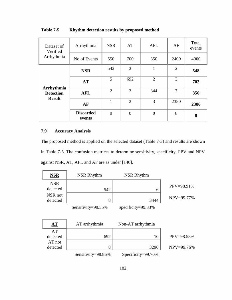
182

Table 7-5 Rhythm detection results by proposed method

Dataset of

Verified

Arrhythmia

Arrhythmia NSR AT AFL AF Total

events

No of Events 550 700 350 2400 4000

Arrhythmia

Detection

Result

NSR 542 3 1 2

548

AT 5 692 2 3

702

AFL 2 3 344 7

356

AF 1 2 3 2380

2386

Discarded

events 0 0 0 8

8

7.9 Accuracy Analysis

The proposed method is applied on the selected dataset (Table 7-3) and results are shown

in Table 7-5. The confusion matrices to determine sensitivity, specificity, PPV and NPV

against NSR, AT, AFL and AF are as under [140].

NSR NSR Rhythm NSR Rhythm

NSR

detected 542 6 PPV=98.91%

NSR not

detected 8 3444 NPV=99.77%

Sensitivity=98.55% Specificity=99.83%

AT AT arrhythmia Non-AT arrhythmia

AT


AT not



183

AFL AFL arrhythmia Non-AFL arrhythmia

AFL


AFL not



AF AF arrhythmia Non-AF arrhythmia

AF


AF not



Table 7-6 shows the accuracy of the proposed system in term of sensitivity, specificity

and PPV and NPV [140].

Table 7-6 Sensitivity, Specificity, PPV and NPV Results

Cardiac

arrhythmia Sensitivity (%) Specificity (%) PPV (%) NPV (%)

NSR 98.55 99.83 98.91 99.77

AT 98.86 99.70 98.58 99.76

AFL 98.29 99.67 96.63 99.84

AF 99.17 99.63 99.75 98.76

184

7.10 Summary

The work presented in this chapter is the continuation of a project aimed at automated

detection of cardiac arrhythmias during an EP study. This work specifically detects and

differentiates among NSR, AT, AFL and AF using atrial IEGMs recorded from HRA and

SVC. After pre-processing of atrial IEGM, Welch spectral estimation method has been

used to estimate DF. A new spectral parameter, APSR has been introduced in this work.

It has been found that APSR can replace RI for ensuring the reliability of DF. Also,

APSR helps in differentiating between AT and AFL in DF range 3~4 Hz and between

AFL and AF in DF range 4~7 Hz. An automated arrhythmia differentiation can facilitate

the patient monitoring during EP study as well as it can be effectively used for additional

therapeutic application by implantable cardioverter defibrillators. The proposed algorithm

has been tested on 4000 verified events and achieved an accuracy of 99.53%.

185

CONCLUSION AND FUTURE WORK

Conclusion

Cardiac Electrophysiology (EP) study is a medical procedure to identify and treat

different types of arrhythmias. The objective of this thesis work was to automate the

detection process for major types of SVT. Both time domain analysis under special

protocols and frequency domain analysis have been applied for differentiation of various

types of SVTs. Real-world IEGM signals were used to check performance of proposed

algorithm. Pre-processing stage is very important for accurate extraction of critical

features. First, IEGMs are passed through noise removal stages, which removes the major

interferences like PLI and EMG noises. The removal of PLI noise is done through an

adaptive state space filter, which has capability to accurately filter out PLI noise. For

removal of EMG noise, Savitzky-golay filter is applied.

After noise removal, the SVT arrhythmia classification has been carried out through two

techniques. First technique is based on temporal features, in which special pacing

protocols are applied and changes in IEGMs are observed to detect reentrant tachycardia,

which include AVNRT and AVRT. Here marking of temporal features is critical; the

onset points of A, H & V waves on selected IEGMs are located to calculate their

temporal relationships. Special attention has been paid for reduction of false positives in

the feature extraction process. The results show that performance of the proposed

algorithm for arrhythmia detection in clinical EPS is comparable to manual diagnostic

procedures. Using the automated detection algorithm in a practical environment can

greatly reduce the manual work done by doctors. The main significance to develop this

186

system is to reduce or minimize the time required by electro physiologist for manual

calculations to find A, V and H waves feature when dealing in time domain.

The second technique is based on non parametric analysis (frequency domain analysis).

While applying frequency domain analysis, the proposed system is able to differentiate

between NSR, AT, AFL and AF. Real-world IEGM signals were used to test the

algorithm. An algorithm has been proposed in which modified Welch method is used for

PSD estimation and a new parameter named as APSR has been introduced which

confirms the reliability of DF and also assist to differentiate among different SVT

arrhythmia. For validation of classification result, the database of AFIC/NIHD and

physionet has been taken as reference and the results were verified by EP specialists.

Future Recommendations

For future researchers in this field, I would like to suggest the following:

1. Atypical AVNRT detection

Features detection in intracardiac domain has been successfully implemented which is

pre-requisite to any arrhythmia detection using temporal relationship of these features

and suitable pacing protocols. Algorithm has been developed for detection of

AVNRT/AVRT using temporal features. AVNRT can be divide into two main types,

which includes typical AVNRT (slow-fast) and atypical AVNRT (fast-slow and slow-

slow). Typical AVNRT is most common of all SVT arrhythmia and its database is easily

available, therefore its algorithm is tested successfully. However database of atypical

AVNRT (fast-slow) was not sufficient to be tested; It is recommended that sufficient

database of atypical AVNRT cases may be collected for detailed testing.

187

2. Sub categorization of AVRT arrhythmia

AVRT arrhythmia is further divided into two main types named as orthdromic (typical)

and antidromic (atypical) AVRT. Atypical AVRT needs to be further explored for

availability of large database and its testing by automated detection algorithm.

3. Hybrid combination of arrhythmia

Sometime it happens that two or more types of arrhythmias are also present whose

signature may be different from individual arrhythmia. Although such combinations are

rare, however these hybrid combinations needs to be further studied in depth for different

possibilities and their automated detection. AVNRT with bystanding accessory pathway

is one such type which often mixed up with antidromic AVRT.

4. Uncommon AV junction related arrhythmia

Algorithm for detection of other types of arrhythmias related to AV junction is required

to be developed. These include Non-paroxysmal junctional tachycardia, focal junctional

tachycardia, junctional tachycardia and WPW.

5. Algorithm to locate accessory pathway

The treatment/cure of AVRT is done by ablating the accessory pathway. Therefore, an

algorithm can be developed for mapping of the accessory pathway in the heart.

6. Sub categories of main SVT arrhythmias

In this work, the major categories of SVT arrhythmia have been differentiated. However,

it can be further extended to differentiate the sub categories of these arrhythmias.

188

7. Algorithm to detect VT arrhythmias

This thesis has laid the ground work for arrhythmia detection algorithm. The work

presented in this research can be modified to design detectors for ventricular Tachycardia

(VT) and its related types.

Acknowledgement

I would like to acknowledge the help and support extended to me for this research work

by

1. EP team of AFIC especially Lt Gen Imran Majeed and Col Azmat

2. Biomedical Dept, AFIC especially Lt Col (R) Mubashar

3. Cardiology Dept, Shifa International hospital especially Dr Habib

189

References

[1] W. H. Organization, "Cardiovascular diseases (CVDs): Fact sheet No. 317. 2011,"

Geneva: World Health Organization Google Scholar, 2011.

[2] E. J. Benjamin, M. J. Blaha, S. E. Chiuve, M. Cushman, S. R. Das, R. Deo, et al.,

"Heart disease and stroke statistics—2017 update: a report from the American

Heart Association," Circulation, vol. 135, pp. e146-e603, 2017.

[3] W. H. Organization, Global status report on noncommunicable diseases 2010:

Geneva: World Health Organization, 2011.

[4] C. D. Mathers and D. Loncar, "Projections of global mortality and burden of

disease from 2002 to 2030," Plos med, vol. 3, p. e442, 2006.

[5] T. F. Luescher and L. van den Berghe, "Circulation: Arrhythmia and

electrophysiology," ed: LIPPINCOTT WILLIAMS & WILKINS 530 WALNUT

ST, PHILADELPHIA, PA 19106-3621 USA, 2008.

[6] S. Goodacre and R. Irons, "Atrial arrhythmias.(ABC of Clinical

Electrocardiography)," British Medical Journal, vol. 324, pp. 594-598, 2002.

[7] R. L. Page, J. A. Joglar, M. A. Caldwell, H. Calkins, J. B. Conti, B. J. Deal, et al.,

"2015 ACC/AHA/HRS guideline for the management of adult patients with

supraventricular tachycardia," Circulation, vol. 133, pp. e506-e574, 2016.

[8] D. G. Katritsis, B. J. Gersh, and A. J. Camm, Clinical cardiology: Current

practice guidelines: OUP Oxford, 2013.

[9] K. W. Lee, N. Badhwar, and M. M. Scheinman, "Supraventricular tachycardia—

part II: history, presentation, mechanism, and treatment," Current problems in

cardiology, vol. 33, pp. 557-622, 2008.

[10] K. W. Lee, N. Badhwar, and M. M. Scheinman, "Supraventricular tachycardia—

part I," Current problems in cardiology, vol. 33, pp. 467-546, 2008.

[11] H. J. Wellens and M. B. Conover, The ECG in emergency decision making: WB

Saunders Company, 2006.

[12] A. L. Goldberger, L. A. Amaral, L. Glass, J. M. Hausdorff, P. C. Ivanov, R. G.

Mark, et al., "Physiobank, physiotoolkit, and physionet components of a new

research resource for complex physiologic signals," Circulation, vol. 101, pp.

e215-e220, 2000.

[13] K. Chatterjee, Cardiology : an illustrated textbook. New Delhi: Jaypee Brothers

Medical Publisher, 2013.

[14] 30 Mar2017). Heart. Available: http://www.innerbody.com/image/card01.html

[15] P. A. Iaizzo, Handbook of cardiac anatomy, physiology, and devices: Springer

Science & Business Media, 2009.

[16] M. S. Thaler, The only EKG book you'll ever need: Lippincott Williams &

Wilkins, 2010.

[17] "action potential," in The American Heritage® New Dictionary of Cultural

Literacy, 3rd ed. Houghton: Houghton Mifflin Company, 2005.

[18] A. Natale and O. Wazni, Handbook of Cardiac Electrophysiology: CRC Press,

2007.

http://www.innerbody.com/image/card01.html

190

[19] R. N. Fogoros. (2013). Electrophysiologic testing. Available:

http://www.dawsonera.com/depp/reader/protected/external/AbstractView/S97811

18399637

[20] P. J. Zimetbaum and M. E. Josephson, Practical clinical electrophysiology:

Lippincott Williams & Wilkins, 2009.

[21] K. Chatterjee, Manual of electrophysiology, 2015.

[22] M. A. Syed, S. V. Raman, and O. P. Simonetti. (2015). Basic principles of

cardiovascular MRI : physics and imaging technique. Available:

http://search.ebscohost.com/login.aspx?direct=true&scope=site&db=nlebk&db=n

labk&AN=1088855

[23] A. E. Buxton, H. Calkins, D. J. Callans, J. P. DiMarco, J. D. Fisher, H. L. Greene,

et al., "ACC/AHA/HRS 2006 key data elements and definitions for

electrophysiological studies and procedures: a report of the American College of

Cardiology/American Heart Association Task Force on Clinical Data Standards

(ACC/AHA/HRS Writing Committee to Develop Data Standards on

Electrophysiology)," Journal of the American College of Cardiology, vol. 48, pp.

2360-2396, 2006.

[24] R. N. Fogoros, Electrophysiologic testing: John Wiley & Sons, 2012.

[25] D. Bosen, "Narrow‐complex tachycardia," Nursing2016, vol. 33, p. 96, 2003.

[26] L. Weinberger, "Wide complex tachycardia," MedEdPORTAL Publications, vol.

7, p. 8499, 2011.

[27] F. D. Murgatroyd, Handbook of cardiac electrophysiology: a practical guide to

invasive EP studies and catheter ablation: Remedica, 2002.

[28] R. Klabunde, Cardiovascular physiology concepts: Lippincott Williams &

Wilkins, 2011.

[29] S. I. Goodacre, R. , "Atrial arrhythmias," British Medical Journal, pp. 594 - 597, 9 Mar

2002.

[30] A. S. Budzikowski. Atrial Tachycardia. Available:

http://emedicine.medscape.com/article/151456-

overview?pa=Yds7%2FnthyijjS35XFzhTe1ExvPR27BmI7vUOKGvDGDU0Ns5

bbFSO18%2Bbe1DtzeTD43mU9jD%2B1DtnxY47OmyybA%3D%3D#a2

[31] V. E. Friedewald, Supraventricular Tachycardia:(SVT/Paroxysmal

Supraventicular Tachycardia/PSVT): Springer, 2016.

[32] A. S. Batra and N. Mohari, "Junctional ectopic tachycardia: current strategies for

diagnosis and management," Progress in Pediatric Cardiology, vol. 35, pp. 49-

54, 2013.

[33] D. McGraw-Hill, "Concise Dictionary of Modern Medicine," ed: The McGraw-

Hill Companies, Inc,. http://medical-dictionary. thefreedictionary. com/(Stand

08.2016), 2002.

[34] M. Boyer and B. A. Koplan, "Atrial flutter," Circulation, vol. 112, pp. e334-e336,

2005.

[35] N. Saoudi, F. COSIO, A. WALDO, S. A. CHEN, Y. Iesaka, M. LESH, et al.,

"Classification of atrial flutter and regular atrial tachycardia according to

electrophysiologic mechanism and anatomic bases: a statement from a joint expert

group from the Working Group of Arrhythmias of the European Society of



http://search.ebscohost.com/login.aspx?direct=true&scope=site&db=nlebk&db=nlabk&AN=1088855

http://search.ebscohost.com/login.aspx?direct=true&scope=site&db=nlebk&db=nlabk&AN=1088855

http://emedicine.medscape.com/article/151456-overview?pa=Yds7%2FnthyijjS35XFzhTe1ExvPR27BmI7vUOKGvDGDU0Ns5bbFSO18%2Bbe1DtzeTD43mU9jD%2B1DtnxY47OmyybA%3D%3D#a2



http://medical-dictionary/

191

Cardiology and the North American Society of Pacing and Electrophysiology,"

Journal of cardiovascular electrophysiology, vol. 12, pp. 852-866, 2001.

[36] A. J. Camm, P. Kirchhof, G. Y. Lip, U. Schotten, I. Savelieva, S. Ernst, et al.,

"Guidelines for the management of atrial fibrillation," European heart journal,

vol. 31, pp. 2369-2429, 2010.

[37] J. E. P. Waktare, "Atrial Fibrillation," Circulation, vol. 106, pp. 14-16, 2002.

[38] C. Tomasi, R. De Ponti, M. Tritto, A. L. Barilli, N. Bottoni, M. Zardini, et al.,

"Simultaneous dual fast and slow pathway conduction upon induction of typical

atrioventricular nodal reentrant tachycardia: electrophysiologic characteristics in a

series of patients," Journal of cardiovascular electrophysiology, vol. 16, pp. 594-

600, 2005.

[39] N. J. Kertesz, R. I. Fogel, and E. N. Prystowsky, "Mechanism of induction of

atrioventricular node reentry by simultaneous anterograde conduction over the

fast and slow pathways," Journal of cardiovascular electrophysiology, vol. 16,

pp. 251-255, 2005.

[40] wikipedia, "Electrocardiography," in wikipedia, ed. (2017, April 10): Wikipedia,

2017.

[41] C. M. Tracy, M. Akhtar, J. P. DiMarco, D. L. Packer, H. H. Weitz, W. L. Winters,

et al., "American College of Cardiology/American Heart Association Clinical

Competence Statement on invasive electrophysiology studies, catheter ablation,

and cardioversion," Circulation, vol. 102, pp. 2309-2320, 2000.

[42] H. Richard. Intro to Intracardiac [Online].

[43] K. Venkatachalam, J. E. Herbrandson, and S. J. Asirvatham, "Signals and signal

processing for the electrophysiologist," Circulation: Arrhythmia and

Electrophysiology, vol. 4, pp. 965-973, 2011.

[44] A. C. Metting van Rijn, A. Peper, and C. A. Grimbergen, "High-quality recording

of bioelectric events," Medical and Biological Engineering and Computing, vol.

28, pp. 389-397, 1990/09/01 1990.

[45] J. Piskorowski, "Digital Q-Varying Notch IIR Filter With Transient Suppression,"

Instrumentation and Measurement, IEEE Transactions on, vol. 59, pp. 866-872,

2010.

[46] B. Widrow, J. R. Glover, Jr., J. M. McCool, J. Kaunitz, C. S. Williams, R. H.

Hearn, et al., "Adaptive noise cancelling: Principles and applications,"

Proceedings of the IEEE, vol. 63, pp. 1692-1716, 1975.

[47] J. Glover, Jr., "Adaptive noise canceling applied to sinusoidal interferences,"

Acoustics, Speech and Signal Processing, IEEE Transactions on, vol. 25, pp. 484-

491, 1977.

[48] C. Chandrakar and M. Kowar, "Denoising ECG signals using adaptive filter

algorithm," International Journal of Soft Computing and Engineering (IJSCE),

vol. 2, pp. 120-123, 2012.

[49] M. Maniruzzaman, K. M. S. Billah, U. Biswas, and B. Gain, "Least-Mean-Square

algorithm based adaptive filters for removing power line interference from ECG

signal," in Informatics, Electronics & Vision (ICIEV), 2012 International

Conference on, 2012, pp. 737-740.

192

[50] H. So, "Adaptive algorithm for sinusoidal interference cancellation," Electronics

Letters, vol. 33, pp. 1910-1912, 1997.

[51] S. M. Martens, M. Mischi, S. G. Oei, and J. W. Bergmans, "An improved

adaptive power line interference canceller for electrocardiography," Biomedical

Engineering, IEEE Transactions on, vol. 53, pp. 2220-2231, 2006.

[52] A. Bazhyna, I. Christov, A. Gotchev, I. Daskalov, and K. Egiazarian, "Powerline

interference suppression in high-resolution ECG," in Computers in Cardiology,

2003, 2003, pp. 561-564.

[53] P. Koseeyaporn, J. Koseeyaporn, and P. Wardkein, "An enhanced adaptive

algorithm for PLI cancellation in ECG signals," in Information, Communications

and Signal Processing, 2009. ICICS 2009. 7th International Conference on, 2009,

pp. 1-5.

[54] I. Badreldin, D. El-Kholy, and A. El-Wakil, "A modified adaptive noise canceler

for electrocardiography with no power-line reference," in Biomedical Engineering

Conference (CIBEC), 2010 5th Cairo International, 2010, pp. 13-16.

[55] I. Badreldin, D. El-Kholy, and A. Elwakil, "Harmonic adaptive noise canceler for

electrocardiography with no power-line reference," in Electrotechnical

Conference (MELECON), 2012 16th IEEE Mediterranean, 2012, pp. 1017-1020.

[56] N. Razzaq, M. Butt, M. Salman, R. Ali, I. Sadiq, K. Munawar, et al., "An

intelligent adaptive filter for fast tracking and elimination of power line

interference from ECG signal," in Computer-Based Medical Systems (CBMS),

2013 IEEE 26th International Symposium on, 2013, pp. 251-256.

[57] R. Acharya, S. M. Krishnan, J. A. Spaan, and J. S. Suri, Advances in cardiac

signal processing: Springer, 2007.

[58] S. M. Alessio, Digital Signal Processing and Spectral Analysis for Scientists:

Concepts and Applications: Springer, 2015.

[59] F. De la Rosa, Harmonics and power systems: CRC Press, 2006.

[60] E. Jacobsen and R. Lyons, "The sliding DFT," Signal Processing Magazine,

IEEE, vol. 20, pp. 74-80, 2003.

[61] M. B. Malik, "State-space recursive least-squares: part I," Signal processing, vol.

84, pp. 1709-1718, 2004.

[62] L. Sörnmo and P. Laguna, Bioelectrical signal processing in cardiac and

neurological applications vol. 8: Academic Press, 2005.

[63] Y.-W. Bai, W.-Y. Chu, C.-Y. Chen, Y.-T. Lee, Y.-C. Tsai, and C.-H. Tsai, "The

combination of Kaiser window and moving average for the low-pass filtering of

the remote ECG signals," in Computer-Based Medical Systems, 2004. CBMS

2004. Proceedings. 17th IEEE Symposium on, 2004, pp. 273-278.

[64] S. Hargittai, "Efficient and fast ECG baseline wander reduction without distortion

of important clinical information," in Computers in Cardiology, 2008, 2008, pp.

841-844.

[65] M. Kaur, B. Singh, J. Ubhi, and S. Rani, "Digital filteration of ecg signals for

removal of baseline drift," in Proceedings of International Conference on

Computer Communication and Management (ICCCM 2011), 2011.

[66] R. Lakhwani, S. Ayub, and J. Saini, "Design and comparison of digital filters for

removal of baseline wandering from ECG signal," in Computational Intelligence

193

and Communication Networks (CICN), 2013 5th International Conference on,

2013, pp. 186-191.

[67] S. Luo and P. Johnston, "A review of electrocardiogram filtering," Journal of

Electrocardiology, vol. 43, pp. 486-496, 2010.

[68] P. Shetty and S. Bhat, "Analysis of various filter configurations on noise

reduction in ECG waveform," International Journal of Computing,

Communications & Instrumentation Engg.(IJCCIE), vol. 1, pp. 88-91, 2014.

[69] J. Van Alste and T. Schilder, "Removal of base-line wander and power-line

interference from the ECG by an efficient FIR filter with a reduced number of

taps," IEEE Transactions on Biomedical Engineering, pp. 1052-1060, 1985.

[70] A. D. BAKHSHI, A. AHMED, S. M. GULFAM, A. KHAQAN, A. YASIN, S.

IQBAL, et al., "Estimation of Baseline Wander Characteristics in ECG Signals

Using Adaptive Transversal Filter and Lomb’s Periodogram Analysis," Przegląd

Elektrotechniczny, vol. 89, pp. 107-110, 2013.

[71] J. R. Gradwohl, E. W. Pottala, M. R. Horton, and J. J. Bailey, "Comparison of two

methods for removing baseline wander in the ECG," in Computers in Cardiology,

1988. Proceedings., 1988, pp. 493-496.

[72] M. Kaur and B. Singh, "Comparison of different approaches for removal of

baseline wander from ECG signal," in Proceedings of the International

Conference & Workshop on Emerging Trends in Technology, 2011, pp. 1290-

1294.

[73] A. Fasano and V. Villani, "ECG baseline wander removal and impact on beat

morphology: A comparative analysis," in Computing in Cardiology Conference

(CinC), 2013, 2013, pp. 1167-1170.

[74] A. Hiasat, M. Al-Ibrahim, and K. Gharaibeh, "Design and implementation of a

new efficient median filtering algorithm," IEE Proceedings-Vision, Image and

Signal Processing, vol. 146, pp. 273-278, 1999.

[75] B. Arvinti, D. Toader, M. Costache, and A. Isar, "Electrocardiogram baseline

wander removal using stationary wavelet approximations," in Optimization of

Electrical and Electronic Equipment (OPTIM), 2010 12th International


[76] M. Dai and S.-L. Lian, "Removal of baseline wander from dynamic

electrocardiogram signals," in Image and Signal Processing, 2009. CISP'09. 2nd

International Congress on, 2009, pp. 1-4.

[77] P. B. Patil and M. S. Chavan, "A wavelet based method for denoising of

biomedical signal," in Pattern Recognition, Informatics and Medical Engineering

(PRIME), 2012 International Conference on, 2012, pp. 278-283.

[78] D. Zhang, "Wavelet approach for ECG baseline wander correction and noise

reduction," in Engineering in Medicine and Biology Society, 2005. IEEE-EMBS

2005. 27th Annual International Conference of the, 2005, pp. 1212-1215.

[79] J. Tang, Q. Zou, Y. Tang, B. Liu, and X.-k. Zhang, "Hilbert-Huang transform for

ECG de-noising," in Bioinformatics and Biomedical Engineering, 2007. ICBBE

2007. The 1st International Conference on, 2007, pp. 664-667.

[80] U. Biswas, A. Das, S. Debnath, and I. Oishee, "ECG signal denoising by using

least-mean-square and normalised-least-mean-square algorithm based adaptive

194

filter," in Informatics, Electronics & Vision (ICIEV), 2014 International


[81] M. Mneimneh, E. Yaz, M. Johnson, and R. Povinelli, "An adaptive Kalman filter

for removing baseline wandering in ECG signals," in Computers in Cardiology,

2006, 2006, pp. 253-256.

[82] A. C. Mugdha, F. S. Rawnaque, and M. U. Ahmed, "A study of recursive least

squares (RLS) adaptive filter algorithm in noise removal from ECG signals," in

Informatics, Electronics & Vision (ICIEV), 2015 International Conference on,

2015, pp. 1-6.

[83] B. Singh, P. Singh, and S. Budhiraja, "Various approaches to minimise noises in

ECG signal: A survey," in Advanced Computing & Communication Technologies

(ACCT), 2015 Fifth International Conference on, 2015, pp. 131-137.

[84] P. Tikkanen, Characterization and application of analysis methods for ECG and

time interval variability data: Oulun yliopisto, 1999.

[85] M. H. Limaye and M. V. Deshmukh, "ECG Noise Sources and Various Noise

Removal Techniques: A Survey."

[86] P. Bhaskar and M. Uplane, "High Frequency Electromyogram Noise Removal

from Electrocardiogram Using FIR Low Pass Filter Based on FPGA," Procedia

Technology, vol. 25, pp. 497-504, 2016.

[87] W. Rose, "Electromyogram analysis," Online course material. University of

Delaware. Retrieved July, vol. 5, p. 2016, 2011.

[88] P. W. Hodges and B. H. Bui, "A comparison of computer-based methods for the

determination of onset of muscle contraction using electromyography,"

Electroencephalography and Clinical Neurophysiology/Electromyography and

Motor Control, vol. 101, pp. 511-519, 1996.

[89] S. L. Joshi, R. A. Vatti, and R. V. Tornekar, "A survey on ECG signal denoising

techniques," in Communication Systems and Network Technologies (CSNT), 2013

International Conference on, 2013, pp. 60-64.

[90] S. Rani, A. Kaur, and J. Ubhi, "Comparative study of FIR and IIR filters for the

removal of Baseline noises from ECG signal," 2011.

[91] W.-h. Lin, M. Y.-M. Wong, L.-n. Pu, and Y.-t. Zhang, "Comparison of median

filter and discrete dyadic wavelet transform for noise cancellation in

electrocardiogram," in Engineering in Medicine and Biology Society (EMBC),

2010 Annual International Conference of the IEEE, 2010, pp. 2395-2398.

[92] M. Z. U. Rahman, R. A. Shaik, and D. Reddy, "Noise cancellation in ECG signals

using computationally simplified adaptive filtering techniques: Application to

biotelemetry," Signal Processing: An International Journal (SPIJ), vol. 3, pp. 1-

12, 2009.

[93] C.-H. Chang, H.-J. Ko, and K.-M. Chang, "Cancellation of high-frequency noise

in ECG signals using adaptive filter without external reference," in Biomedical

Engineering and Informatics (BMEI), 2010 3rd International Conference on,

2010, pp. 787-790.

[94] S. Hargittai, "Savitzky-Golay least-squares polynomial filters in ECG signal

processing," in Computers in Cardiology, 2005, 2005, pp. 763-766.

195

[95] J. S. Sørensen, L. Johannesen, U. S. L. Grove, K. Lundhus, J.-P. Couderc, and C.

Graff, "A comparison of IIR and wavelet filtering for noise reduction of the

ECG," in Computing in Cardiology, 2010, 2010, pp. 489-492.

[96] M. Khan, F. Aslam, T. Zaidi, and S. A. Khan, "Wavelet based ecg denoising

using signal-noise residue method," in Bioinformatics and Biomedical

Engineering,(iCBBE) 2011 5th International Conference on, 2011, pp. 1-4.

[97] R. W. Schafer, "What is a Savitzky-Golay filter?[lecture notes]," IEEE Signal

processing magazine, vol. 28, pp. 111-117, 2011.

[98] R. MacDonald, J. Jenkins, R. Arzbaecher, and R. Throne, "A software trigger for

intracardiac waveform detection with automatic threshold adjustment," in

Computers in Cardiology 1989, Proceedings., 1989, pp. 167-170.

[99] S. Greenhut, R. MacDonald, J. Jenkins, and R. Arzbaecher, "Real-time computer

acquisition, analysis, and display of electrophysiology studies," in Computers in

Cardiology 1990, Proceedings., 1990, pp. 573-576.

[100] L. Pang, K. Danehorn, I. Tchoudovski, and A. Bolz, "Automatic identification of

cardiac activations in the multi-channel Intracardiac ECGs," 2006.

[101] P. De Chazal, M. O'Dwyer, and R. B. Reilly, "Automatic classification of

heartbeats using ECG morphology and heartbeat interval features," IEEE

Transactions on Biomedical Engineering, vol. 51, pp. 1196-1206, 2004.

[102] P. de Chazal and R. B. Reilly, "A patient-adapting heartbeat classifier using ECG

morphology and heartbeat interval features," IEEE Transactions on Biomedical

Engineering, vol. 53, pp. 2535-2543, 2006.

[103] C. Ye, B. V. Kumar, and M. T. Coimbra, "Heartbeat classification using

morphological and dynamic features of ECG signals," IEEE Transactions on

Biomedical Engineering, vol. 59, pp. 2930-2941, 2012.

[104] P. de Chazal and R. B. Reilly, "Automatic classification of ECG beats using

waveform shape and heart beat interval features," in Acoustics, Speech, and

Signal Processing, 2003. Proceedings.(ICASSP'03). 2003 IEEE International

Conference on, 2003, pp. II-269.

[105] S. Raj, K. Maurya, and K. C. Ray, "A knowledge-based real time embedded

platform for arrhythmia beat classification," Biomedical Engineering Letters, vol.

5, pp. 271-280, 2015.

[106] I. Murthy and G. D. Prasad, "Analysis of ECG from pole-zero models," IEEE

transactions on biomedical engineering, vol. 39, pp. 741-751, 1992.

[107] S. Mehta, S. Saxena, and H. Verma, "Computer-aided interpretation of ECG for

diagnostics," International journal of systems science, vol. 27, pp. 43-58, 1996.

[108] M. L. Ahlstrom and W. J. Tompkins, "Automated high-speed analysis of Holter

tapes with microcomputers," IEEE Transactions on Biomedical Engineering, pp.

651-657, 1983.

[109] A. D. Bakhshi, M. A. Maud, K. M. Aamir, and A. Loan, "Aggregate spectrogram

based classification of Holter ECG signals for wireless sensor networks," in

Emerging Technologies (ICET), 2012 International Conference on, 2012, pp. 1-6.

[110] S. Saksena and A. J. Camm, Electrophysiological Disorders of the Heart: Expert

Consult: Elsevier Health Sciences, 2011.

196

[111] H. Vänttinen, J. Nousiainen, P. Mäkynen, and J. Malmivuo, "Windows software

for cardiac electrophysiology studies and ablation monitoring," Computer

methods and programs in biomedicine, vol. 61, pp. 221-231, 2000.

[112] S. Choi and Z. Jiang, "Comparison of envelope extraction algorithms for cardiac

sound signal segmentation," Expert Systems with Applications, vol. 34, pp. 1056-

1069, 2008.

[113] J. Liu, W. Liu, H. Wang, T. Tao, and J. Zhang, "A novel envelope extraction

method for multichannel heart sounds signal detection," in 2011 International

conference on computer science and information technology, IPCSIT, 2012, pp.

630-638.

[114] C. Jarne, "Simple empirical algorithm to obtain signal envelope in three steps,"

arXiv preprint arXiv:1703.06812, 2017.

[115] L. A. Borowitz and W. J. Combs, "Implantable medical device with his-purkinje

activity detection," ed: Google Patents, 2010.

[116] P. W. Macfarlane and T. D. V. Lawrie, Comprehensive electrocardiology: theory

and practice in health and disease vol. 2: Pergamon, 1989.

[117] A.-R. LeBlanc and A. Mokrane, "Improved beat-to-beat timing measurements of

His-bundle signal," IEEE transactions on biomedical engineering, vol. 41, pp.

1168-1177, 1994.

[118] F. Kusumoto, "Procedural Issues for Electrophysiologic Studies: Vascular Access,

Cardiac Chamber Access, and Catheters," Understanding Intracardiac EGMs and

ECGs, pp. 1-14.

[119] W. Nafees, B. Riaz, N. Razzaq, W. Iftikhar, and T. Zaidi, "Classification of Atrio-

Ventricular Reentrant Tachycardia using intracardiac signals," in Bioinformatics

and Bioengineering (BIBE), 2013 IEEE 13th International Conference on, 2013,

pp. 1-5.

[120] A. C. Rankin, F. R. Quinn, and A. P. Rae, "Clinical cardiac electrophysiology," in

Comprehensive Electrocardiology, ed: Springer, 2010, pp. 1133-1161.

[121] S. Z. Mahmoodabadi, A. Ahmadian, M. Abolhassani, J. Alireazie, and P. Babyn,

"ECG arrhythmia detection using fuzzy classifiers," in Fuzzy Information

Processing Society, 2007. NAFIPS'07. Annual Meeting of the North American,

2007, pp. 48-53.

[122] B. Raghavendra, D. Bera, A. S. Bopardikar, and R. Narayanan, "Cardiac

arrhythmia detection using dynamic time warping of ECG beats in e-healthcare

systems," in World of Wireless, Mobile and Multimedia Networks (WoWMoM),

2011 IEEE International Symposium on a, 2011, pp. 1-6.

[123] B. Kamousi, B. Lin, A. Al-Ahmad, H. Hsia, P. Zei, A. Natale, et al., "A

covariance-based algorithm: a novel technique for rhythm discrimination in

ICDs," in Engineering in Medicine and Biology Society, 2008. EMBS 2008. 30th

Annual International Conference of the IEEE, 2008, pp. 5478-5481.

[124] D. G. Katritsis and A. J. Camm, "Classification and differential diagnosis of

atrioventricular nodal re-entrant tachycardia," Europace, vol. 8, pp. 29-36, 2006.

[125] D. G. Katritsis and A. J. Camm, "Atrioventricular nodal reentrant tachycardia,"

Circulation, vol. 122, pp. 831-840, 2010.

197

[126] M. Al Mehairi, S. Al Ghamdi, K. Dagriri, and A. Al Fagih, "Simultaneous

antegrade dual AV node conduction initiates AV nodal re-entrant tachycardia (a

rare initiation mechanism)," Journal of the Saudi Heart Association, vol. 25, pp.

35-37, 2013.

[127] Y. I. Alihanoglu, B. S. Yildiz, D. I. Kilic, H. Evrengul, and S. Kose, "Clinical and

Electrophysiological Characteristics of Typical Atrioventricular Nodal Reentrant

Tachycardia in the Elderly–Changing of Slow Pathway Location With Aging–,"

Circulation Journal, vol. 79, pp. 1031-1036, 2015.

[128] S. Dora, N. Namboodiri, A. Valaparambil, and J. Tharakan, "Induction of

atrioventricular nodal reentry tachycardia with intravenous adenosine," Singapore

medical journal, vol. 48, pp. e130-2, 2007.

[129] P. Weismüller, S. Kuly, B. Brandts, K. Kattenbeck, C. Ranke, and H. J. Trappe,

"Is electrical stimulation during administration of catecholamines required for the

evaluation of success after ablation of atrioventricular node re-entrant

tachycardias?," Journal of the American College of Cardiology, vol. 39, pp. 689-

694, 2002.

[130] K. Tanaka and Y. Watanabe, "Type A Wolff-Parkinson-White Syndrome

Generating an Antidromic Atrioventricular (AV) Reentrant Tachycardia (AVRT)

and an Orthodromic AVRT with a Long RP Interval Initiated only after

Incomplete Impairment of an AV Accessory Pathway," Journal of Arrhythmia,

vol. 27, pp. 137-144, 2011.

[131] M. E. Josephson, Clinical cardiac electrophysiology: techniques and

interpretations: Lippincott Williams & Wilkins, 2008.

[132] C. Buttà, A. Tuttolomondo, D. Di Raimondo, G. Milio, S. Miceli, M. T. Attanzio,

et al., "The supraventricular tachycardias: Proposal of a diagnostic algorithm for

the narrow complex tachycardias," Journal of cardiology, vol. 61, pp. 247-255,

2013.

[133] U. N. Kumar, R. K. Rao, and M. M. Scheinman, "The 12-lead electrocardiogram

in supraventricular tachycardia," Cardiology clinics, vol. 24, pp. 427-437, 2006.

[134] G. D. Veenhuyzen, F. R. Quinn, S. B. Wilton, R. Clegg, and L. B. Mitchell,

"Diagnostic pacing maneuvers for supraventricular tachycardias: Part 2," Pacing

and Clinical Electrophysiology, vol. 35, pp. 757-769, 2012.

[135] G. D. Veenhuyzen, F. R. Quinn, S. B. Wilton, R. Clegg, and L. B. Mitchell,

"Diagnostic pacing maneuvers for supraventricular tachycardia: part 1," Pacing

and Clinical Electrophysiology, vol. 34, pp. 767-782, 2011.

[136] H. Richard, Arrhythmias, 2007.

[137] D. A. Pijnappels, J. van Tuyn, T. A. de Vries, A. van der Laarse, E. E. van der

Wall, M. J. Schalij, et al., "Electrophysiology: Basic."

[138] N. Varma, "Left ventricular conduction delays induced by right ventricular apical

pacing: effect of left ventricular dysfunction and bundle branch block," Journal of

cardiovascular electrophysiology, vol. 19, pp. 114-122, 2008.

[139] H. Calkins, J. Sousa, R. El-Atassi, S. Rosenheck, M. De Buitleir, W. H. Kou, et

al., "Diagnosis and cure of the Wolff-Parkinson-White syndrome or paroxysmal

supraventricular tachycardias during a single electrophysiologic test," New

England Journal of Medicine, vol. 324, pp. 1612-1618, 1991.

198

[140] M. Sokolova and G. Lapalme, "A systematic analysis of performance measures

for classification tasks," Information Processing & Management, vol. 45, pp. 427-

437, 2009.

[141] S. Hargittai, "Is it possible to detect atrial fibrillation by simply using RR

intervals?," in Computing in Cardiology Conference (CinC), 2014, 2014, pp. 897-

900.

[142] G. Hayes and P. D. Teal, "Real-time detection of atrial fibrillation using a low-

power ECG monitor," in Computing in Cardiology Conference (CinC), 2013,

2013, pp. 743-746.

[143] J. R. Schaefer, D. Leussler, L. Rosin, D. Pittrow, and T. Hepp, "Improved

detection of paroxysmal atrial fibrillation utilizing a software-assisted

electrocardiogram approach," PloS one, vol. 9, p. e89328, 2014.

[144] J. F. Martin-Garcia, I. Mora-Jiménez, A. Garcia-Alberola, and J. L. Rojo-Alvarez,

"Cardiac arrhythmia discrimination using evolutionary computation," in

Computing in Cardiology Conference (CinC), 2014, 2014, pp. 121-124.

[145] J. SLOCUM, A. SAHAKIAN, and S. SWIRYN, "Computer Discrimination of

Atrial Fibrillation and Regular Atrial Rhythms from Intra‐Atrial Electrograms,"

Pacing and Clinical Electrophysiology, vol. 11, pp. 610-621, 1988.

[146] K. M. Ropella, A. V. Sahakian, J. Baerman, and S. Swiryn, "Effects of

procainamide on intra-atrial [corrected] electrograms during atrial fibrillation:

implications [corrected] for detection algorithms," Circulation, vol. 77, pp. 1047-

1054, 1988.

[147] J. Slocum, A. Sahakian, and S. Swiryn, "Diagnosis of atrial fibrillation from

surface electrocardiograms based on computer-detected atrial activity," Journal of

electrocardiology, vol. 25, pp. 1-8, 1992.

[148] M. A. Wood, P. Moskovljevic, B. S. Stambler, and K. A. Ellenbogen,

"Comparison of bipolar atrial electrogram amplitude in sinus rhythm, atrial

fibrillation, and atrial flutter," Pacing and Clinical Electrophysiology, vol. 19, pp.

150-156, 1996.

[149] K. Tateno and L. Glass, "Automatic detection of atrial fibrillation using the

coefficient of variation and density histograms of RR and ΔRR intervals,"

Medical and Biological Engineering and Computing, vol. 39, pp. 664-671, 2001.

[150] J. Millet-Roig, J. Rieta, V. Zarzoso, A. Cebrian, F. Castells, C. Sanchez, et al.,

"Surface-ECG atrial activity extraction via blind source separation: spectral

validation," in Computers in Cardiology, 2002, 2002, pp. 605-608.

[151] R. JJ, J. Millet-Roig, V. Zarzoso, F. Castells, С. Sánchez, R. García-Civera, et al.,

"Atrial Fibrillation, Atrial Flutter and Normal Sinus Rhythm Discrimination by

Means of Blind Source Separation and Spectral Parameters Extraction."

[152] J. Ng and J. J. Goldberger, "Understanding and interpreting dominant frequency

analysis of AF electrograms," Journal of cardiovascular electrophysiology, vol.

18, pp. 680-685, 2007.

[153] R. Latchamsetty and A. G. Kocheril, "Review of dominant frequency analysis in

atrial fibrillation," Arbor, vol. 1001, p. 48103, 2009.

199

[154] V. B. Traykov, R. Pap, and L. Sághy, "Frequency domain mapping of atrial

fibrillation-methodology, experimental data and clinical implications," Current

cardiology reviews, vol. 8, p. 231, 2012.

[155] T. H. Everett IV, L.-C. Kok, R. H. Vaughn, J. R. Moorman, and D. E. Haines,

"Frequency domain algorithm for quantifying atrial fibrillation organization to

increase defibrillation efficacy," Biomedical Engineering, IEEE Transactions on,

vol. 48, pp. 969-978, 2001.

[156] T. H. Everett, J. G. Akar, L.-C. Kok, J. R. Moorman, and D. E. Haines, "Use of

global atrial fibrillation organization to optimize the success of burst pace

termination," Journal of the American College of Cardiology, vol. 40, pp. 1831-

1840, 2002.

[157] P. Sanders, O. Berenfeld, M. Hocini, P. Jaïs, R. Vaidyanathan, L.-F. Hsu, et al.,

"Spectral analysis identifies sites of high-frequency activity maintaining atrial

fibrillation in humans," Circulation, vol. 112, pp. 789-797, 2005.

[158] A. Arenal, T. Datino, L. Atea, F. Atienza, E. González-Torrecilla, J. Almendral, et

al., "Dominant frequency differences in atrial fibrillation patients with and

without left ventricular systolic dysfunction," Europace, vol. 11, pp. 450-457,

2009.

[159] W.-C. Tsai and Y.-J. Lin, "The Frequency Analysis and the Atrial Fibrillation," J

Biocatal Biotransformation 1: 2. doi: 10.4172/2324-9099.1000 e108, 2012.

[160] Y.-J. Lin, C.-T. Tai, T. Kao, H.-W. Tso, S. Higa, H.-M. Tsao, et al., "Frequency

analysis in different types of paroxysmal atrial fibrillation," Journal of the

American College of Cardiology, vol. 47, pp. 1401-1407, 2006.

[161] J. J. Rieta, F. Castells, C. Sánchez, V. Zarzoso, and J. Millet, "Atrial activity

extraction for atrial fibrillation analysis using blind source separation," IEEE

Transactions on Biomedical Engineering, vol. 51, pp. 1176-1186, 2004.

[162] A. J. Camm, P. Kirchhof, G. Y. Lip, U. Schotten, I. Savelieva, S. Ernst, et al.

(2010). Guidelines for the management of atrial fibrillation. 31.

[163] K. Nagashima, Y. Okumura, I. Watanabe, T. Nakai, K. Ohkubo, T. Kofune, et al.,

"Effects of inter-electrode spacing on complex fractionated atrial electrograms

and dominant frequency detection," Journal of interventional cardiac

electrophysiology, vol. 34, pp. 51-57, 2012.

[164] G. W. Botteron and J. M. Smith, "A technique for measurement of the extent of

spatial organization of atrial activation during atrial fibrillation in the intact

human heart," Biomedical Engineering, IEEE Transactions on, vol. 42, pp. 579-

586, 1995.

[165] J. Ng, A. H. Kadish, and J. J. Goldberger, "Technical considerations for dominant

frequency analysis," Journal of cardiovascular electrophysiology, vol. 18, pp.

757-764, 2007.

[166] P. D. Welch, "The use of fast Fourier transform for the estimation of power

spectra: A method based on time averaging over short, modified periodograms,"

IEEE Transactions on audio and electroacoustics, vol. 15, pp. 70-73, 1967.

[167] S.-a. A. Sheikh, A. Z. Majoka, K. U. Rehman, N. Razzaq, and T. Zaidi,

"Nonparametric Spectral Estimation Technique to Estimate Dominant Frequency

200

for Atrial Fibrillation Detection," Journal of Signal and Information Processing,

vol. 6, p. 266, 2015.

[168] W. Li, C. Yang, Y. Wang, D. Wang, Y. Chen, and Z. Wu, "Several insights into

the preprocessing of electrograms in atrial fibrillation for dominant frequency

analysis," BioMedical Engineering OnLine, vol. 15, p. 1, 2016.

[169] M. S. Bartlett, "Smoothing periodograms from time series with continuous

spectra," Nature, vol. 161, pp. 686-687, 1948.

[170] K. Barbe, R. Pintelon, and J. Schoukens, "Welch method revisited: nonparametric

power spectrum estimation via circular overlap," IEEE Transactions on signal

processing, vol. 58, pp. 553-565, 2010.

[171] E. C. Ifeachor and B. W. Jervis, Digital signal processing: a practical approach:

Pearson Education, 2002.

[172] K. J. Blinowska and J. Zygierewicz, Practical Biomedical Signal Analysis Using

MATLAB®: CRC Press, 2011.

[173] A. V. Panfilov and A. V. Holden, Computational biology of the heart: Wiley,

1997.

201

All Praises and Thanks be to Allah

CARDIAC SIGNAL PROCESSING FOR CLASSIFICATION OF ...

Documents

Transcript of CARDIAC SIGNAL PROCESSING FOR CLASSIFICATION OF ...