2Students graph data to examine seasonal and long-term atmospheric carbon dioxide trends over the past 45 years. They will predict future carbon dioxide emissions based on the graph. Students also examine graphs of historical temperature and carbon dioxide data. The activity closes with a discussion of ways to reduce carbon dioxide emissions.

Carbon Dioxide Trends

19clim

ate chan

ge

Inquiry/Critical Thinking Questions

What are some activities that emit car-•bon dioxide into Earth’s atmosphere?What have been the major trends in •atmospheric carbon dioxide levels?How is carbon dioxide related to tem-•peratures on Earth?How can we reduce future carbon diox-•ide emissions?

Objectives

Students will:Identify processes that contribute to •carbon dioxide emissionsGraph carbon dioxide emissions•Predict future carbon dioxide trends•Assess the relationship between at-•mospheric carbon dioxide and global surface temperaturesBrainstorm ways to reduce carbon diox-•ide emissions

Time Required

50 minutes

Key Concepts

Carbon dioxide emissions•Greenhouse effect•

Subject Areas

Science (Life, Environmental, Physical, •Earth)Mathematics•

National Standards Alignment

National Science Education Standards (NSES)

Standard A: Science as Inquiry •Standard C: Life Science•Standard D: Earth and Space Science •Standard F: Science in Personal and •Social Perspectives

Materials/Preparation

Graph paper, 1 sheet per student pair •(alternately, use a graphing program such as Microsoft Excel)Handout: CO• 2 Dataset, 1 per student pairOverhead: long-term carbon dioxide •and temperature trends

C A R B O N D I OX I D E T R E N D S

20

faci

ng

th

e fu

ture

ActivityIntroduction

Ask students to recall which gases 1. are involved in the greenhouse effect. (water vapor, carbon dioxide, methane, and nitrous oxide, along with man-made gases) Tell students that today they’ll be exploring historical trends in carbon dioxide emissions. Explain that carbon dioxide (CO2) is an important greenhouse gas that has been linked to many human activities.Ask students if they can name some 2. activities, human or otherwise, that might add CO2 to our atmosphere. (burning fossil fuels, cutting trees, burning wood, and cellular respiration all release CO2)

Steps

Divide the class into pairs. 1. Give each pair 1 sheet of graph paper 2. and 1 CO2 dataset.

Note: This dataset from Mauna Loa is the most complete and accurate CO2 dataset in the world. CO2 is measured in parts per million; 316 parts per million means that for every 1 million particles in the atmosphere, 316 of those are carbon dioxide molecules.

Have students graph the data. (Year 3. should be on the x-axis and CO2 emissions on the y-axis. The scale should be appropriate for the data.) Students

can use a computer graphing program as an alternative to graphing by hand.

Lesson Variation: To shorten this activ-ity, have students only graph the num-bers for May.

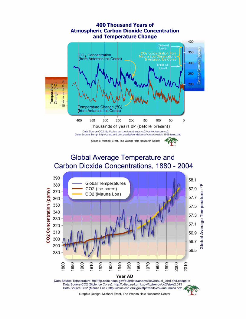
Ask students to predict an average 4. carbon dioxide concentration for the year 2020 and put a star on their graph to represent that number on their graph.Reconvene the class to view and 5. discuss the graphs from the Woods Hole Research Center on historical temperature and CO2 trends. Ask students to explain what they see in these graphs. Where is the Mauna Loa data shown in these graphs? When does the most recent warming trend begin?Bring the class together for a discussion 6. using the following reflection questions.

Reflection

What might account for differences in 1. the CO2 concentrations measured in May and October of each year? (Lower values represent increased CO2 uptake during the summer when plants are photosynthesizing more; high values represent decreased photosynthesis during the winter.) How could we take advantage of those 2. natural periods of increased CO2

C A R B O N D I OX I D E T R E N D S21

climate ch

ang

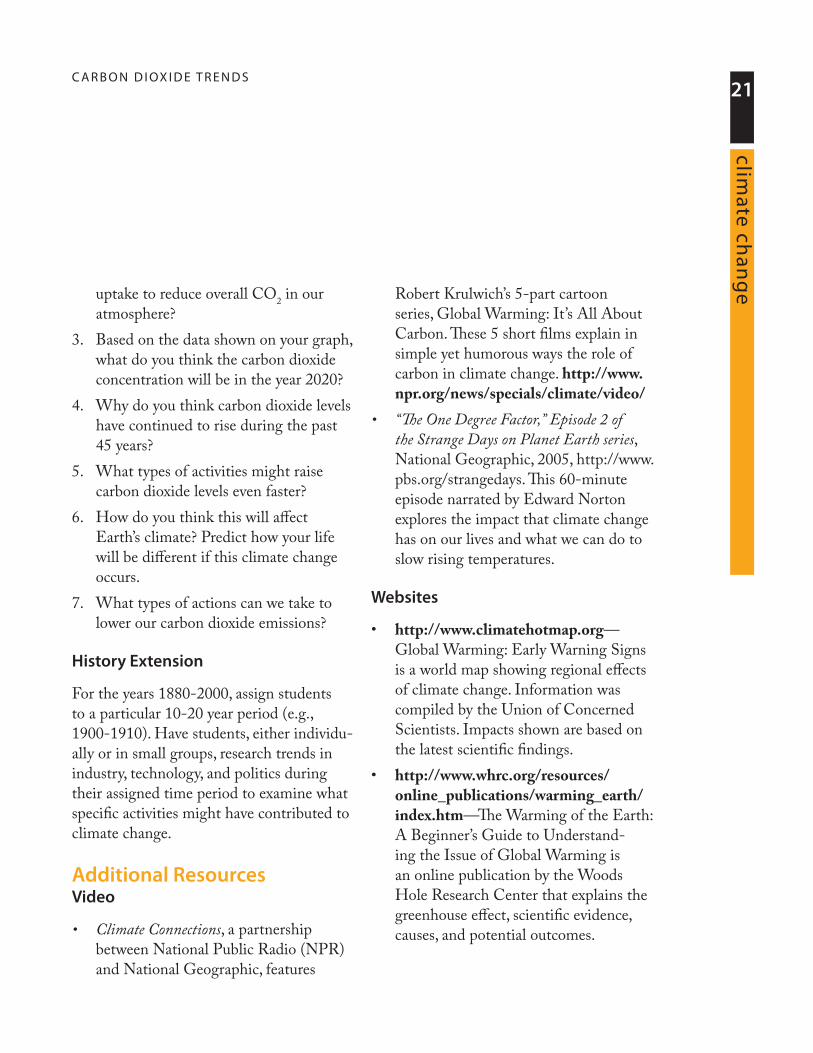
euptake to reduce overall CO2 in our atmosphere?Based on the data shown on your graph, 3. what do you think the carbon dioxide concentration will be in the year 2020? Why do you think carbon dioxide levels 4. have continued to rise during the past 45 years?What types of activities might raise 5. carbon dioxide levels even faster? How do you think this will affect 6. Earth’s climate? Predict how your life will be different if this climate change occurs.What types of actions can we take to 7. lower our carbon dioxide emissions?

History Extension

For the years 1880-2000, assign students to a particular 10-20 year period (e.g., 1900-1910). Have students, either individu-ally or in small groups, research trends in industry, technology, and politics during their assigned time period to examine what specific activities might have contributed to climate change.

Additional ResourcesVideo

Climate Connections• , a partnership between National Public Radio (NPR) and National Geographic, features

Robert Krulwich’s 5-part cartoon series, Global Warming: It’s All About Carbon. These 5 short films explain in simple yet humorous ways the role of carbon in climate change. http://www.npr.org/news/specials/climate/video/ “The One Degree Factor,” Episode 2 of •the Strange Days on Planet Earth series, National Geographic, 2005, http://www.pbs.org/strangedays. This 60-minute episode narrated by Edward Norton explores the impact that climate change has on our lives and what we can do to slow rising temperatures.

Websites

http://www.climatehotmap.org• —Global Warming: Early Warning Signs is a world map showing regional effects of climate change. Information was compiled by the Union of Concerned Scientists. Impacts shown are based on the latest scientific findings. http://www.whrc.org/resources/ •online_publications/warming_earth/index.htm—The Warming of the Earth: A Beginner’s Guide to Understand-ing the Issue of Global Warming is an online publication by the Woods Hole Research Center that explains the greenhouse effect, scientific evidence, causes, and potential outcomes.

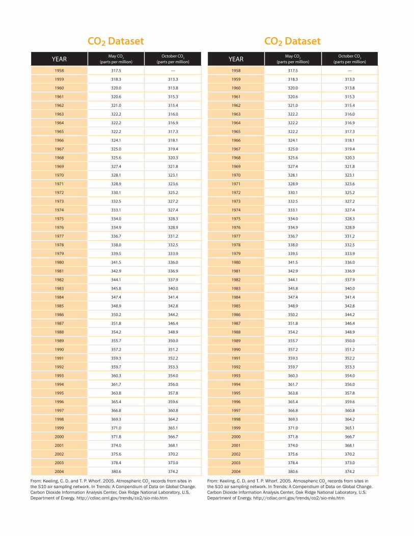
CO2 Dataset CO2 Dataset

From: Keeling, C. D. and T. P. Whorf. 2005. Atmospheric CO2 records from sites in the S10 air sampling network. In Trends: A Compendium of Data on Global Change. Carbon Dioxide Information Analysis Center, Oak Ridge National Laboratory, U.S. Department of Energy. http://cdiac.ornl.gov/trends/co2/sio-mlo.htm

YEAR May CO2 (parts per million)

October CO2

(parts per million)

1958 317.5 ---

1959 318.3 313.3

1960 320.0 313.8

1961 320.6 315.3

1962 321.0 315.4

1963 322.2 316.0

1964 322.2 316.9

1965 322.2 317.3

1966 324.1 318.1

1967 325.0 319.4

1968 325.6 320.3

1969 327.4 321.8

1970 328.1 323.1

1971 328.9 323.6

1972 330.1 325.2

1973 332.5 327.2

1974 333.1 327.4

1975 334.0 328.3

1976 334.9 328.9

1977 336.7 331.2

1978 338.0 332.5

1979 339.5 333.9

1980 341.5 336.0

1981 342.9 336.9

1982 344.1 337.9

1983 345.8 340.0

1984 347.4 341.4

1985 348.9 342.8

1986 350.2 344.2

1987 351.8 346.4

1988 354.2 348.9

1989 355.7 350.0

1990 357.2 351.2

1991 359.3 352.2

1992 359.7 353.3

1993 360.3 354.0

1994 361.7 356.0

1995 363.8 357.8

1996 365.4 359.6

1997 366.8 360.8

1998 369.3 364.2

1999 371.0 365.1

2000 371.8 366.7

2001 374.0 368.1

2002 375.6 370.2

2003 378.4 373.0

2004 380.6 374.2

From: Keeling, C. D. and T. P. Whorf. 2005. Atmospheric CO2 records from sites in the S10 air sampling network. In Trends: A Compendium of Data on Global Change. Carbon Dioxide Information Analysis Center, Oak Ridge National Laboratory, U.S. Department of Energy. http://cdiac.ornl.gov/trends/co2/sio-mlo.htm

YEAR May CO2 (parts per million)

October CO2

(parts per million)

1958 317.5 ---

1959 318.3 313.3

1960 320.0 313.8

1961 320.6 315.3

1962 321.0 315.4

1963 322.2 316.0

1964 322.2 316.9

1965 322.2 317.3

1966 324.1 318.1

1967 325.0 319.4

1968 325.6 320.3

1969 327.4 321.8

1970 328.1 323.1

1971 328.9 323.6

1972 330.1 325.2

1973 332.5 327.2

1974 333.1 327.4

1975 334.0 328.3

1976 334.9 328.9

1977 336.7 331.2

1978 338.0 332.5

1979 339.5 333.9

1980 341.5 336.0

1981 342.9 336.9

1982 344.1 337.9

1983 345.8 340.0

1984 347.4 341.4

1985 348.9 342.8

1986 350.2 344.2

1987 351.8 346.4

1988 354.2 348.9

1989 355.7 350.0

1990 357.2 351.2

1991 359.3 352.2

1992 359.7 353.3

1993 360.3 354.0

1994 361.7 356.0

1995 363.8 357.8

1996 365.4 359.6

1997 366.8 360.8

1998 369.3 364.2

1999 371.0 365.1

2000 371.8 366.7

2001 374.0 368.1

2002 375.6 370.2

2003 378.4 373.0

2004 380.6 374.2