CapturingFlexibleHeterogeneousUtility Curves ...s-space.snu.ac.kr/bitstream/10371/67972/1/Capturing...

MANAGEMENT SCIENCEVol. 53, No. 2, February 2007, pp. 340–354issn 0025-1909 �eissn 1526-5501 �07 �5302 �0340

informs ®

doi 10.1287/mnsc.1060.0616©2007 INFORMS

Capturing Flexible Heterogeneous UtilityCurves: A Bayesian Spline Approach

Jin Gyo KimCollege of Business Administration, Seoul National University, Gwanak-Gu, Shillim 9 Dong,

Seoul 151-742, Korea, [email protected]

Ulrich MenzefrickeJoseph L. Rotman School of Management, University of Toronto, 105 St. George Street,

Toronto, Ontario, Canada, M5S 3E6, [email protected]

Fred M. FeinbergStephen M. Ross School of Business, University of Michigan, 701 Tappan Street,

Ann Arbor, Michigan 48109, [email protected]

Empirical evidence suggests that decision makers often weight successive additional units of a valuedattribute or monetary endowment unequally, so that their utility functions are intrinsically nonlinear or irreg-

ularly shaped. Although the analyst may impose various functional specifications exogenously, this approach isad hoc, tedious, and reliant on various metrics to decide which specification is “best.” In this paper, we developa method that yields individual-level, flexibly shaped utility functions for use in choice models. This flexibilityat the individual level is accomplished through splines of the truncated power basis type in a general additiveregression framework for latent utility. Because the number and location of spline knots are unknown, we usethe birth-death process of Denison et al. (1998) and Green’s (1995) reversible jump method. We further showhow exogenous constraints suggested by theory, such as monotonicity of price response, can be accommodated.Our formulation is particularly suited to estimating reaction to pricing, where individual-level monotonicityis justified theoretically and empirically, but linearity is typically not. The method is illustrated in a conjointapplication in which all covariates are splined simultaneously and in three panel data sets, each of which hasa single price spline. Empirical results indicate that piecewise linear splines with a modest number of knots fitthese data well, substantially better than heterogeneous linear and log-linear a priori specifications. In termsof price response specifically, we find that although aggregate market-level curves can be nearly linear or log-linear, individuals often deviate widely from either. Using splines, hold-out prediction improvement over thestandard heterogeneous probit model ranges from 6% to 14% in the scanner applications and exceeds 20% inthe conjoint study. Moreover, “optimal” profiles in conjoint and aggregate price response curves in the scannerapplications can differ markedly under the standard and the spline-based models.

Key words : choice models; utility theory; heterogeneity; splines; Bayesian methods; Markov chain Monte CarloHistory : Accepted by Jagmohan S. Raju, marketing; received August 29, 2002. This paper was with the authors32 months for 3 revisions.

1. Heterogenous Utility and FlexibleFunctional Forms

Previous studies of choice models have typically as-sumed that utility can be linked to covariates lin-early, usually via a fixed functional form exogenouslyimposed by the analyst. These assumptions are moti-vated largely by methodological convenience in termsof model structure and estimation, as well as post hocinterpretability of the underlying parameterization.There is, however, substantial theoretical and empir-ical justification from several disciplines in favor ofutility functions of various, often irregular, shapes. Inthe economics literature, many studies on “flexible”functional forms (Wales 1977, Caves and Christensen

1980) in demand systems have supported utility non-linearity at the aggregate level. Such flexibility iscrucial in gauging response to price, in particular,a finding echoed in marketing (Abe 1998, Bell andLattin 2000) and psychology (Wu and Gonzalez 1996,Gonzalez and Wu 1999).The estimation of flexible individual-specific func-

tions in empirical studies using choice models haslargely been neglected, hampered by methodologi-cal difficulties. One difficulty—of needing to exoge-nously impose a particular functional specificationfor latent utility—raises a number of problems ofits own. The first such problem is ordinarily theory-dependent: Which particular specification should beimposed? Because utility itself is unobserved, there is

340

Kim, Menzefricke, and Feinberg: Capturing Flexible Heterogeneous Utility Curves: Bayesian Spline ApproachManagement Science 53(2), pp. 340–354, © 2007 INFORMS 341

seldom any overriding theoretical justification for onefunctional specification over another, other than pureparsimony. This may be, in part, why linear specifi-cations have come to assume something of a defaultrole. A second problem follows from the first: Whentheory fails to suggest a particular functional speci-fication, which should be explored? A trial-and-errorapproach is time consuming and raises questionsof overfitting; it also requires specification of func-tional families from which one might reasonably drawcandidates. A final problem concerns how the ana-lyst might choose among various candidate specifica-tions; that is, which test procedures should be used?Because different empirical applications favor dif-ferent parameterizations, theoretical generalizationsacross studies may be difficult to come by.In this paper, we propose a nonparametric, spline-

based model to investigate flexible utility functions forchoice models, with a particular empirical emphasison capturing price response. The presented methodallows one to (1) model utility functions at the indi-vidual rather than at the aggregate level, (2) exam-ine the degree of cross-sectional variation in utilityfunction shape, and (3) better understand the truerelationship among specific covariates (particularly,price), observed choice probabilities, and market-levelresponse. Throughout, we stress that it is not strictlinearity, per se, that our approach is meant to relax.Rather, it is the need to prespecify a particular func-tional form for individual-level utility.We test the proposed formulation against those

commonly applied in prior literature in a varietyof settings: a conjoint application for the design ofa small durable and three scanner panel data setsof varying characteristics. The conjoint application,although stemming from a design with fixed within-attribute levels, allows each of six input variables tobe splined simultaneously. The scanner applicationsallow for the assessment of individual-level priceresponse curves, where the spline “knots” are house-hold-specific. In all applications, we find that piece-wise-linear splines give rise to curves that appear tocapture covariate effects well, particularly for price.Gains from the application of splines are substan-tial, not only in terms of Bayesian measures of modelfit but in the managerially critical metric of predic-tive accuracy in hold-out samples. Moreover, responseestimates systematically differ when strict assump-tions of price response linearity are relaxed to mono-tonicity, as we do here.The remainder of this paper is organized as fol-

lows. Section 2 reviews key literature that bears onthe assessment of latent utility, with particular regardto individual-level specifications and price response

linearity. Section 3 incorporates truncated power basistype splines into a heterogeneous probit choice frame-work, and describes specification issues, identifica-tion, and Bayesian estimation. Section 4 presents fourapplications and the comparative results of a vari-ety of utility specifications on the assessment of priceresponse. Finally, §5 discusses both theoretical andmanagerial implications of our suggested approach,as well as avenues for future research.

2. Modeling Flexible Utility andPricing Effects

Choice models typically assume that multiattributesystems link observed choices to covariates (e.g.,prices or environmental variables). However, the ex-tant literature has been largely silent on estimatingconsumer-specific, flexible functions for latent utility.Gonzalez and Wu (1999) found substantial evidencefor complex utility shapes at both the aggregate andindividual levels; moreover, they detailed the substan-tial methodological problems in measuring them atthe individual level, even in a controlled setting andusing parametric representations. To our knowledge,obtaining such measurements using field data notsubject to experimental controls is an open question.Marketing studies provide consistent evidence that

response to environmental variables, particularlyprice, can be nonlinear, with substantial individual-level variation. For example, Kalyanaram and Little(1989) demonstrated the existence of a range ofprices in which consumers are very nearly insensi-tive to price changes, and Gupta and Cooper (1992)reported a similar effect for price discounts. Account-ing for complex pricing effects has been among areasto which splines have been successfully applied.Kalyanam and Shively (1998) applied a stochasticspline methodology to weekly unit sales for multiplebrands and categories, finding wide shape variation,although their model was not designed to account forhousehold-level effects.A number of studies have addressed nonlinear util-

ity formulations nonparametrically. Abe (1998) pro-posed a nonparametric additive model to estimatea binary logit model utility function, albeit only atthe aggregate level, finding it to be nonlinear. Brieschet al. (2002) used a nonparametric representation tostudy whether consumers react differently to pricereductions versus larger deal discounts, discoveringdeviations from linearity in deal effects across fourcategories. Shively et al. (2000) proposed a nonpara-metric model for the relationship between consumerpreference and a set of explanatory covariates andfound that several such relationships (four in 24)in their study were decidedly nonlinear. In conjoint

Kim, Menzefricke, and Feinberg: Capturing Flexible Heterogeneous Utility Curves: Bayesian Spline Approach342 Management Science 53(2), pp. 340–354, © 2007 INFORMS

modeling, the use of piecewise linear, heterogeneousutility functions of multiple attributes is quite com-mon (Lenk et al. 1996, Andrews et al. 2002).In this paper, we conflate the objectives of these var-

ious studies, allowing for complex functional shapesat the individual level, where utilities themselves arelatent. This goal is analogous to that of Bell andLattin (2000), who found that unless response hetero-geneity is appropriately accounted for, measurementsof important aspects of consumer behavior—in theircase, reliance on reference prices—could go dramat-ically awry. Our empirical applications will examinewhether presumptions about the shape of individual-level price response may be altering inferences aboutmarket-level strategy. In this way, we seek to freemanagerial decisions, specifically regarding optimalpricing strategy, from artifacts of specific functionalassumptions about how individuals translate productattributes and prices into relative preference. In thenext section, we present a spline-based model formu-lated with this specific goal in mind.

3. Model Specification3.1. Multinomial Probit ModelLet yht = j denote the event that individual h (h =1� � � � �H� chooses alternative j j = 1� � � � � J � on choiceoccasion t t = 1� � � � � Th�. Let xhjt denote individual h’sk-dimensional vector of discrete explanatory vari-ables (e.g., feature, display) for alternative j on choiceoccasion t. Throughout, we use “choice occasion”as a generic label for purchase occasion (in scannerpanel data) or choice task (in conjoint data). Supposethat there are M continuous explanatory variablesvhjt = vhjt�1� � � � � vhjt�M�′. Then, individual h’s utilityfor alternative j on choice occasion t is assumed to fol-low an additive regression specification (Hastie andTibshirani 1990),

uhjt = x′hjt�h +M∑

m=1f h

mvhjtm�+ �hjt� (1)

where f hm•� is an unknown, possibly nonlinear, func-

tion of vhjtm and �hjt is an error term. A more detaileddiscussion of our specification for f h

m is given in §3.2.To complete the model specification, let uht =

uh1t� � � � �uhJt�′ denote a J -dimensional vector of latent

utilities, let xht = xh1t� � � � � xhJt�′ denote a J ×k covariate

matrix, define �hjt = ∑Mm=1 f

hmvhjtm�, �ht = �h1t� � � � �

�hJt�′, and let �ht = �h1t� � � � � �hJt�

′ be a J -dimensionalnormal random vector with mean vector 0 and covari-ance matrix �u. Summarizing, our model is

yht = j if uhjt =maxuh1t� � � � �uhJt�� such that

uht = xht�h +�ht + �ht� �ht ∼NJ 0��u��(2)

where NJ �� denotes a J -dimensional normal dis-tribution with mean vector � and covariance matrix �.The resulting choice probabilities for the multinomialprobit model are given by the J -fold integral,

phjt = pyht = j � �h��ht��u�

=∫Ah1t

· · ·∫AhJt

nJ uht � xht�h +�ht��u� duht�

j = 1� � � � � J � (3)

where nJ u �� denotes a J -variate normal densityfor the vector u with mean vector � and covariancematrix �. Furthermore, Ahit is the interval −�uhjt�if i = j and −�� if i = j . This specification suffersfrom two well-known identification problems: loca-tion invariance and scale invariance. Our approach toresolving these identification problems is slightly dif-ferent for the conjoint and scanner panel data appli-cations that we describe in §4.In the conjoint data application, we let the last op-

tion, J , be a “no-choice” option. We set the utility ofthe no-choice option to uhJt ≡ 0; therefore, we mustintroduce an intercept for each individual, �h0, thatmeasures the individual’s intrinsic utility preferenceof choice versus no choice. Thus, we have

uhjt = �h0+ x′hjt�h1+�hjt + �hjt�

j = 1� � � � � J − 1� and (4)

uhJt ≡ 0�

where x′hjt and �hjt are described after (1) and before(2), and where the covariance matrix for the J − 1�-dimensional error term, �ht = �h1t� � � � � �h� J−1� t�

′, is aJ − 1�-dimensional identity matrix, denoted IJ−1.In the scanner data applications, we suppose that

there are alternative-specific intercepts for the J alter-natives and also a number of additional binary vari-ables; we will include two such in our applications:feature advertising and display. The portion of theresulting J × J + 2� matrix xht that corresponds tothe alternative-specific intercepts is a J × J � iden-tity matrix. To deal with the location identificationproblem, we arbitrarily pick one of the alternatives(say, J ) and drop the J th column of this identitymatrix; the corresponding alternative-specific inter-cept is therefore unnecessary, and thus the other J −1alternative-specific intercepts are measured relative toalternative J . We note that this will affect interpreta-tions of alternative-specific intercepts across models,as both the intercept in question and the “base” usedfor identification must jointly be taken into account.There are several methods available to handle thescale invariance problem in the scanner data applica-tions. Chib and Greenberg (1998) and McCulloch et al.(2000) provide thorough discussions.


3.2. Incorporating Splines into the ModelIn this section, we first describe our use of splines toapproximate the function f h

m in (1) and then some esti-mation issues related to splines. To incorporate flexi-bly shaped utility functions, we use a nonparametricapproach without strong functional assumptions tomodel f h

m. It is well known that a continuous functionmay be arbitrarily well approximated by a piecewisepolynomial function with a sufficiently large numberof knots (cf. Wegman and Wright 1983). Specifically,we let each f h

m•� be a spline function with a truncatedpower basis (Denison et al. 1998, Lindstrom 2002),also known as a “one-sided basis” (Schumaker 1981,p. 112),

f hmvhjtm� =

lm∑n=1

�hmnvhjtm − shm0�n+

+qhm∑i=1

�hm� l+ivhjtm − shmi�lm+ (5)

for vhjtm ∈ shm�0� shm�qhm+1!, where w+ = max0�w�,w0

+ = Iw ≥ 0�, qhm is the number of interior knotsfor individual h for the mth spline function, lm isthe order of the spline, $�hmi% are individual-specificspline coefficients, and $shmi%, arranged in ascend-ing order, are individual-specific interior knot pointswith boundary knots, shm�0 and shm�qhm+1, for the mthspline. Here, Ia� is the usual indicator function forthe event a.In our applications, we found linear splines to per-

form better than splines of higher order, andwe restrictour discussion here to linear splines.1 Thus, we use

f hmvhjtm� = �hm1vhjtm − shm0�+

+qhm∑i=1

�hm�1+ivhjtm − shmi�+� (6)

Note that, for identification purposes, we do notinclude an intercept term in (5) or (6), accommodatingone as needed through �h in (1).Let us now turn to some estimation issues related

to the spline functions. Because the uhjt are unknownlatent variables, it is very difficult to choose a rea-sonable knot configuration for each individual inadvance. A key feature of our model is that it endoge-nously settles on an appropriate knot configuration,leading to the difficult problem of spline estimationwith varying knots (see Wegman and Wright 1983

1 Details of the MCMC sampler for linear and higher order splines,various prior settings, and all full conditionals are included inthe online appendix to this paper (provided in the e-companion),and in Kim et al. (2007). The electronic companion to this paperis available as part of the online version that can be found athttp://mansci.journal.informs.org/.

for a review). The linear spline function model in (6)requires the estimation of two sets of parameters:(1) the knot configuration, that is, the number andlocation of knots, qhm and shm�1� � � � � shm�qhm

; and (2) thespline coefficients, �hm�1� � � � � �hm�1+qhm

.We use Markov chain Monte Carlo (MCMC) simu-

lation to estimate the spline functions. Our notationfor the parameters that describe the household-specific knot configurations is as follows:• qhm ∈ $0�1� � � � �Qm% denotes the possible number

of interior knots for f hm•� given Qm candidate knots,

• �hm = $Dhm1� � � � �DhmQm% denotes a set of Qm can-

didate interior knots, and• )hm = $shm�1� � � � � shm�qhm

% denotes a set of qhm inte-rior knots chosen from �hm.The appendix describes the hierarchical structure

for the regression coefficients �h in (1) and �h =�h0��

′h1�

′ in (4), and the prior distributions for allparameters.

3.2.1. Monotonicity and Knot Configuration. Re-searchers often seek to place constraints on individual-specific utility shapes. These can come about for avariety of reasons, including those imposed by theory,rationality, or previous findings. For example, eco-nomic theory suggests that the spline reflecting theeffect of price be monotonically decreasing. In ourapplications, we will thus require

f hmvhjtm�≥ f h

mv∗hjtm� if vhjtm ≤ v∗

hjtm� (7)

Note that (7) leads to several separate inequality con-straints that must be jointly satisfied. The multivariatenormal random-effects probit, by contrast, allows forthe possibility that some individual-level “draws” arenonmonotonic or even nondecreasing.The knot configuration for each individual at each

MCMC iteration is sampled from a collection of pre-specified candidate knot points; we take up how toarrive at this candidate set in our applications. We usea special discrete version of Green’s (1995) reversible-jump Metropolis-Hastings algorithm in our MCMCsimulation. Green’s method allows the number andlocation of knots to vary across iterations by allowing“births” and “deaths” among them, a critical featureto which we will return in our applications.

4. Empirical ApplicationsThe proposed model is illustrated for two widelypopular applications of choice models in marketing:choice-based conjoint and scanner panel data. Theconjoint application is chosen to demonstrate howto estimate multiple spline functions simultaneously.The three scanner data applications are pursued toshow how to solve the varying knot problem forindividual-level utility splines where there is a rela-tively large number of candidate knots.


The conjoint data set contains six attributes, eachwith five levels, thus limiting the number of pos-sible knots and predetermining their potential loca-tions. We estimate the spline-based model on threeseparate scanner data sets, comparing fit and hold-out performance to that of the standard multinomialprobit (MNP) model for both linear and log-linearprice specifications. We note that the log-price formis directly suggested by economic theory, given opti-mal consumer budget allocation (Allenby and Rossi1991). For both types of application, we focus mainlyon parameter estimates relevant to, and implicationsof, splines. Because our empirical results supportedlinear splines in all four applications, we present onlythose results; all others are available in the onlineappendix.

4.1. Application I: Choice-Based ConjointWe model conjoint choice data for bathroom scalescollected by the Optimal Design Engineering Labora-tory at the University of Michigan (see Michalek et al.2005 for further details regarding study design andmaterials). The design consisted of six attributes—weight capacity, platform aspect ratio, platform area,interval gap between one-pound markings, size ofprinted numbers, and price—each with five levels.Specific levels for each of these attributes appear inTable 1. Each of 184 subjects completed an onlineseries of 50 fixed tasks, each including three productprofiles and a no-choice option; thus, H = 184 andJ = 4. For the purpose of out-of-sample validation, wedivided the full data set into training, y, and predic-tion data sets, �y. The prediction data consisted of thelast 10 choice observations for each subject, so thatthe number of observations in the training data set isTh = 40 ∀h.Because none of the six attributes is purely cate-

gorical, we introduced a separate spline for each, soM = 6 in (1). To aid in graphical comparability, wedivided by the lowest value for each attribute, leav-ing the transformed largest values distinct; see the lastcolumn in Table 1. Splines were then introduced overthese rescaled levels.

4.1.1. Model Comparison. We estimated severaldifferent models. First, we estimated a baseline model,M0, the random effects probit commonly applied in

Table 1 Attributes and Their Levels in the Conjoint Study

m Attributes Unit Levels Rescaled levels

1 Weight capacity lbs. 200; 250; 300; 350; 400 1; 1.25; 1.50; 1.75; 2.002 Platform aspect ratio length/width 6/8; 7/8; 1; 8/7; 8/6 1; 1.17; 1.33; 1.52; 1.783 Platform area in.2 100; 110; 120; 130; 140 1; 1.10; 1.20; 1.30; 1.404 Interval mark gap in. 0.063; 0.094; 0.125; 0.156; 0.188 1; 1.49; 1.98; 2.45; 2.985 Size of number in. 0.75; 1.00; 1.25; 1.50; 1.75 1; 1.33; 1.66; 2.00; 2.336 Price $ 10; 15; 20; 25; 30 1; 1.50; 2.00; 2.50; 3.00

choice-based conjoint:

uhjt = �h0+ x′hjt�h1+ �hjt�

j = 1� � � � � J − 1� and (8)

uhJt ≡ 0�

where �ht = �h1t� � � � � �h� J−1� t�′ ∼ NJ−10� I�. Note that

M0 is actually less restrictive than a spline model, asit allows any sort of relationship between the part-worths for a particular attribute. We will examineempirically whether this flexibility helps or hampershold-out performance.Because uhJt ≡ 0 and �h0 is included in the spec-

ification for uhjt , we define xhjt so that the “effect”of the first level of each attribute is zero. Therefore,xhjt was a 24-dimensional vector, consisting of fourdummy variables for the second to the fifth levels foreach attribute. Thus, �h0 measures the utility of thechoice option at the lowest values for all attributesover the no-choice option. The parameters of the base-line model are �h0 and �h1. The relevant hierarchicalstructure and prior distributions are as in item (1) inthe appendix; the chosen values of the priors for M0were g0 = 0, c0 = 20, a0 = b0 = 0�5, g1 = 024, C1 =W1 =20I24, and r1 = 2. We also estimated the linear splinemodel S described after (6):

uhjt = �h0+6∑

m=1f h

mvhjtm�+ �hjt�

j = 1� � � � � J − 1� and (9)

uhJt ≡ 0�

where �ht = �h1t� � � � � �h� J−1� t�′ ∼ NJ−10� I�, as de-

scribed previously.The set �hm of candidate knots for the mth spline

(m = 1� � � � �6) consisted of the three interior levelsof the corresponding attribute. The exterior levels(here, the first and the fifth) serve as boundary knots.Because the profile stimuli sets were identical acrosssubjects, so are these candidate knots. Thus, the num-ber of interior knots qhm ∈ $0�1�2�3% ∀h�m. In addi-tion, the monotonicity constraint was imposed on theprice spline, f h

6 •�, although the other splines wereunconstrained.


Table 2 Model Performance in the Conjoint Study

Training data Prediction data

Log of integrated log of Log of posterior Correctly predicted:Model likelihood BFM0 � • predictive distribution hit rate (%)

M0 (Heterogeneous traditional probit) −5�828�70 0 −2�361�80 48.08S (Heterogeneous linear spline probit) −4�451�67 1�377�03 −1�895�57 59.42

The parameters for our spline model in the conjointapplication are �h0 and the parameters characterizingthe splines. The appendix describes the hierarchicalstructure for these parameters and the prior distri-butions. We chose the prior parameter values g0 = 0,c0 = 20, and a0 = b0 = 0�5; these are identical to thosefor M0. Furthermore, the prior distributions for thespline coefficients �

qhm�)hm�

hm� i had parameters am = 0 andbm = 10 m = 1� � � � �6�. Finally, the distribution forthe number of internal knots qhm was Poisson (withparameter /m = 3) truncated at 3, the maximum num-ber of internal knots. Empirically, we observed littlesubstantive dependence on /m for nearby values orrelative to a uniform prior.After 10,000 iterations, all models seemed to con-

verge; the proportion of sampled quantities thatpassed the Geweke convergence statistics rangedfrom 77.6% to 100%. Parameter inferences were basedon an additional 30,000 iterations. For all spline mod-els, the subject-specific knot configurations were wellmixed, as indicated by examining individual-leveltrace plots.2 To choose between two models, B1 andB2, we calculate the Bayes factor, BFB1�B2

, the ratio ofthe two respective integrated likelihoods. For suchcomputations, we applied Genz’ (1992, 1993) adaptiveMonte Carlo and Lattice Rule methods. Fortran codesfor these methods are available from Genz.To assess the relative performance of the spline

models for the prediction data set, we computed twoquantities:1. The predictive density at the observed values �y

of the prediction data set, p�y � y� = ∫p�y � ��p� �

y� d�, where � denotes all unknown parameters ofthe given model, p�y � �� denotes the density of �ygiven the parameters �, and p� � y� denotes the pos-terior distribution for � given the training data set y.2. The proportion of correctly predicted purchases

for the given model, this so-called “hit rate” wasobtained by first sampling latent utilities for eachpurchase observation in �y, given �, at each MCMCiteration, computing the proportion of all purchasesfor which the chosen alternative was the one with

2 As an informal check on convergence, we recomputed all reportedquantities using the first and last third of the iterations used forinference; this was done for all four included applications. Differ-ences were substantively minor and never significant.

maximal utility and then averaging these proportionsacross iterations.Table 2 presents the integrated likelihoods and pre-

dictive inferences. By either measure, the linear splinemodel S was decisively preferred to the traditionalheterogeneous probit model. This result may seemsurprising, given the great improvement—23.6%—inhold-out hit rate for the spline-based models. How-ever, we believe that it may be explained as follows.Note that the prediction data set relied on part-worthvalues that were deliberately included in the trainingset. However, this was relatively less “informative”for some respondents than others because they tendedto select the no-choice option or simply avoided cer-tain attribute levels among their choices. In suchcases, the spline model could leverage informationon other attribute levels for that particular respondent,whereas the traditional heterogeneous probit (M0)could do so only for other respondents (through theacross-subjects attribute correlation). In other words,the spline model provides an explicit mechanism fora “smoothing” of part-worths so that the values ofpoorly estimated attribute levels can be improved viainterpolation across MCMC runs; M0, although lessrestricted, lacks such a mechanism.An extreme case—avoided in our study by de-

sign—is one in which the prediction stimuli includelevels never tested in the training data. In such acase, M0 might have to resort to ad hoc (linear) inter-polation using adjacent values only, whereas spline-based models can interpolate based on all levelsfor that attribute. We speculate that a spline-basedmodel might perform well as an update mechanismfor adaptive conjoint studies, although we have notexplored that possibility here.Because the linear spline model performed best, we

examine it in greater detail in the following section.

4.1.2. Estimation Results for the Linear SplineModel, S. It is instructive to examine estimates result-ing from S, relative to those from M0, and their rel-ative implications. For brevity, we consider variationin knot configuration, function shape, and optimaldesign using various summary measures and tests.

Interior Knot Configurations. The knot configurationwas quite varied across subjects, and we explore thisissue in greater depth in our scanner applications.Let us temporarily set aside the posterior uncertainty


Figure 1 Conjoint Data—Histogram of Modal Number of Interior KnotsAcross Subjects

0.8

0.7

0.6

0.5

0.4

0.3

0.2

0.1

00 1 2 3

Number of interior knots

Prop

ortio

n of

sub

ject

s

Weight capacityPlatform aspect ratioPlatform areaInterval mark gapNumber sizePrice

about the number of knots and focus instead onthe modal number of interior knots for each subjectand attribute. Figure 1 presents a histogram of thesesubject-specific modal numbers for each of the sixattributes.First, consider attributes m = 4 and m = 6, inter-

val mark gap, and price. The modal number was 0for 1.6% and 25% of subjects, respectively; for thelinear spline model S, this lack of knots implies lin-ear (increasing or decreasing) part-worth curves forrelatively few subjects. Conversely, the modal num-ber was greater than zero for a sizable proportion ofsubjects, 98.4% and 75.0%; these subjects thus appearto have nonlinear part-worth curves for these twoattributes. For the other four attributes, there wasnot even a single subject whose modal number ofinterior knots was zero, suggesting that all subjectsexhibited some degree of nonlinearity for these fourattributes. Intriguingly, of all six attributes, price hadby far the largest proportion of modal knot zeros, asper Figure 1; for these individuals, a linear specifica-tion would apparently be most appropriate for priceamong the six attributes.Summarizing, Model S suggests considerable vari-

ation in the number of interior knots across subjects,and it provides very strong evidence in favor of non-linearity in part-worth curves for all attributes (withthe possible exception of price for about one quarterof respondents). Of course, M0 also does not presumelinearity, so the superior performance of S cannot beattributed directly to allowing for nonlinear response.But M0 imposes a sort of foundational nonlinearity:Each attribute level is estimated separately, so near-linear relations across them occur only by happen-stance, not as a built-in feature of the model of whichthe estimation can avail. In practice, the analyst usingM0 is likely to interpolate between adjacent levelswhen necessary, but not between nonadjacent levelsbecause a distinct utility value is indicated at each

level. Under the linear spline model S, however, aslong as the number of internal knots is not at itsmaximum value (here, three), the utility values atsome of these fixed levels would, in fact, be the lin-ear interpolant of its adjacent values. The estimatedpart-worth curves may thus be smoother under S thanunderM0. Let us now examine this possibility and theshapes of individual part-worth curves under variousmodels.

Disaggregate Spline Part-Worth Curves. It is straight-forward to use the MCMC output to estimate in-dividual-specific splines. Because knot number andlocation can change from one iteration to another, theresulting curve of posterior means is not necessarilya linear spline curve; it is likely smoother. Using thelinear spline model, Figure 2 presents posterior meanpart-worth curves for two randomly selected subjectsfor weight capacity and price. The solid and the thinlines in Figure 2 represent the posterior mean part-worth curves under S and M0, respectively; dottedlines enveloping the part-worth curves indicate pos-terior 5th and 95th percentile part-worth curves. Atthe lowest (base) level of each attribute, the poste-rior variance of the part-worth curve is zero because,

Figure 2 Conjoint Data—Individual-Level Spline �S� and Benchmark�M0� Part-Worth Curves

Weight capacity

–2

–1

0

1

2

3

4

200 lb 250 lb 300 lb 350 lb 400 lb

h = 6

SplineBenchmark[5 percentile, 95 percentile]

Price

Part

-wor

thPa

rt-w

orth

–3

–2

–1

0

1

$10 $15 $20 $25 $30

h = 3


for identification purposes, the curve measures differ-ences relative to this base.As conjectured, each of the posterior mean part-

worth curves under S appears smoother than theanalogous curves under M0, which often tend tozigzag across attribute levels, as evidenced by h= 6for weight capacity. Except for the price spline underS, no constraints were imposed, so this differencein smoothness (and, on occasion, monotonicity) is agenuine substantive difference between the two mod-els’ individual-level part-worth predictions. We reportinformally that a similar pattern is evident through-out the subject pool.Whereas it is not meaningful to compare the ver-

tical distances between the two posterior mean part-worth curves in Figure 2 at different levels of anattribute, we can compare the shapes of the two poste-rior mean part-worth curves: It is smoother under thespline model than model M0. One must bear in mindthat the posterior variation around such curves canbe large, even with many observations per subject. Assuch, the analyst should make individual-level infer-ences with caution, perhaps eschewing them entirelyin favor of aggregate inferences, which we take upnext.

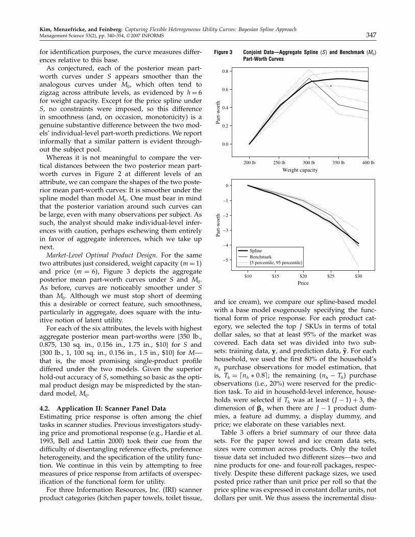
Market-Level Optimal Product Design. For the sametwo attributes just considered, weight capacity m= 1�and price m = 6�, Figure 3 depicts the aggregateposterior mean part-worth curves under S and M0.As before, curves are noticeably smoother under Sthan M0. Although we must stop short of deemingthis a desirable or correct feature, such smoothness,particularly in aggregate, does square with the intu-itive notion of latent utility.For each of the six attributes, the levels with highest

aggregate posterior mean part-worths were {350 lb.,0.875, 130 sq. in., 0.156 in., 1.75 in., $10} for S and{300 lb., 1, 100 sq. in., 0.156 in., 1.5 in., $10} for M—that is, the most promising single-product profilediffered under the two models. Given the superiorhold-out accuracy of S, something so basic as the opti-mal product design may be mispredicted by the stan-dard model, M0.

4.2. Application II: Scanner Panel DataEstimating price response is often among the chieftasks in scanner studies. Previous investigators study-ing price and promotional response (e.g., Hardie et al.1993, Bell and Lattin 2000) took their cue from thedifficulty of disentangling reference effects, preferenceheterogeneity, and the specification of the utility func-tion. We continue in this vein by attempting to freemeasures of price response from artifacts of overspec-ification of the functional form for utility.For three Information Resources, Inc. (IRI) scanner

product categories (kitchen paper towels, toilet tissue,

Figure 3 Conjoint Data—Aggregate Spline �S� and Benchmark �M0�

Part-Worth Curves

Weight capacity

Part

-wor

thPa

rt-w

orth

0.0

0.2

0.4

0.6

0.8

200 lb 250 lb 300 lb 350 lb 400 lb

Price

–5

–4

–3

–2

–1

0

$10 $15 $20 $25 $30

SplineBenchmark[5 percentile, 95 percentile]

and ice cream), we compare our spline-based modelwith a base model exogenously specifying the func-tional form of price response. For each product cat-egory, we selected the top J SKUs in terms of totaldollar sales, so that at least 95% of the market wascovered. Each data set was divided into two sub-sets: training data, y, and prediction data, �y. For eachhousehold, we used the first 80% of the household’snh purchase observations for model estimation, thatis, Th = �nh ∗ 0�8�; the remaining nh − Th� purchaseobservations (i.e., 20%) were reserved for the predic-tion task. To aid in household-level inference, house-holds were selected if Th was at least J − 1�+ 3, thedimension of �h when there are J − 1 product dum-mies, a feature ad dummy, a display dummy, andprice; we elaborate on these variables next.Table 3 offers a brief summary of our three data

sets. For the paper towel and ice cream data sets,sizes were common across products. Only the toilettissue data set included two different sizes—two andnine products for one- and four-roll packages, respec-tively. Despite these different package sizes, we usedposted price rather than unit price per roll so that theprice spline was expressed in constant dollar units, notdollars per unit. We thus assess the incremental disu-


Table 3 Summary of IRI Scanner Panel Data Sets

Total number ofpurchase observations

ObservedCategory Product size J H price range Training data Prediction data

Paper towels 1 roll 6 133 $0.33, $1.32 2,131 479Toilet tissue 1 and 4 rolls 11 198 $0.38, $2.45 5,123 1�197Ice cream 64 oz 7 81 $0.49, $4.49 1,159 252

tility of each additional monetary unit, size differ-ences being at least partially mitigated via productdummies.3

4.2.1. Model Comparison. We compared severalmodels for the three scanner data sets, with pricebeing the focal and only continuous variable; thus,M = 1. Furthermore, we imposed monotonicity onall spline-based price response curves. The predictorvariable vector xhjt needed for the spline model in (1)was a vector of J − 1 product dummies, a featuread dummy, and a display dummy. To ensure iden-tifiability, we did not introduce a dummy variablefor the last product, J . The dimension of the designmatrix xht , required in (2), was (J × k), with k = J + 1.For simplicity, as in the conjoint application, each dataset had a common spline order for all households,that is, lh1 = l. We again estimated the proposed splinemodels, Sl, for increasing l until there was no furtherimprovement in fit.As benchmarks, we estimated two models popular

in the literature: the linear, M0, and log-linear, Mlog,price response models. As in our conjoint applica-tion, M0 was the standard probit model, where xhjt

consisted of J − 1 product dummies, one feature addummy, one display dummy, and price. For both M0

and Mlog, the dimension of the regression coefficientvector was k = J + 2.As noted before, using the approach of McCulloch

et al. (2000) and an unrestricted covariance matrix �u,the MCMC simulation did not always converge for allour models (i.e., M0, Mlog, and S), particularly for theproduct dummy elements in ��. Because most house-holds in the data sets purchased a sharply restrictedsubset of the available products, �� and �u for infre-quently purchased products may have been weaklyidentified. As there were no convergence problemsfor �� when �u was specified to be a correlation

3 There were empirical justifications for this choice as well. First,prices across the two different sizes did overlap: Price ranges were$0.38–$0.63 and $0.48–$2.45 for one- and four-roll products, respec-tively; standard tests using the individual prices as inputs did notshow means to differ significantly p > 0�1� across the two sizes.Second, all models subsequently reported fit better when actualposted prices were used instead of unit prices: BFactual price, unit priceranged from 304.9 to 365.1 across all models.

matrix, we use the correlation form for �u in all modelcomparisons.4

The relevant hierarchical structure and the priordistributions are given in the appendix. The prior dis-tributions for ��, ��, and �u had the following values:

g� = 0k� C� = 20Ik� r� = 2�W� = 20Ik� m= 5� and C= 4IJ �

Note that the values for m and C led to a prior distri-bution for �u centered at IJ , with reasonably diffusepriors for the off-diagonal entries of �u; specifically,the [mean± 2× std. dev.] interval for the off-diagonalelements under the prior was −1�26�1�26!, coveringthe range −1�1� of possible correlation values.To determine the prior distribution for a house-

hold’s knot locations, we first obtained a household-specific set of candidate knots for the price splines,�h1, based on the household’s observed prices in thetraining data: After listing the distinct prices for allalternatives and all purchase occasions, we selectedQh1 candidate knots by subdividing the distinct pricesinto Qh1 + 1 equal parts. By doing so, all intervalsbounded by two adjacent interior knots had at leastone price observation; this was important, as it isimpossible to make inferences regarding intervalsdevoid of observations. Discretizing the set of can-didate knot locations resulted in a discrete proposaldistribution for knot locations, simplifying the appli-cation of the birth-death steps in our reversible-jumpalgorithm.For simplicity, we set the number of candidate

knots Qh1 to be the same for all households in agiven data set: 9, 11, and 10 for the paper towel, toi-let tissue, and ice cream data sets, respectively. Asa practical complication, price ranges differed in thetraining and prediction data sets, even for a givenhousehold. To ensure that predictions could be madefor the prediction data set under the monotonicityconstraint across the relevant price range, we let shm�0and shm�qh+1 be the minimal and maximal observedprices in the whole data set, as opposed to the training

4 We do not believe the correlation matrix to be an especially severerestriction as �u allows for correlated utilities, and does not imposeIIA; see, for example, Chib and Greenberg (1998).


data alone. These minimal and maximal values wereused only for the prediction tasks; inferences on pricesplines should be made only in the range of pricesobserved in the training data set.The prior distribution for a household’s interior

knot number was Poisson with parameter /1 = 3,implying a reasonably diffuse prior. Simulations sug-gested that inferences were not very sensitive tochoice of /1, nor to using a flat prior. Given a valuefor the interior number of knots, qh1, the prior fora household’s knot locations was a random samplefrom the

(Qh1qh1

)possible knot configurations from �h1.

Finally, the prior distribution for each spline coeffi-cient �

qh1� )h1�

h1� i was normal with mean a1 = 0 and vari-ance b1 = 10.For all models, the first 20,000 iterations of the

MCMC simulation were a burn-in period; parametricinferences were based on an additional 20,000 itera-tions. The proportion of parameters among �� and ��

that passed the Geweke convergence statistics rangedfrom 82.9% to 91.1% for spline models; the household-specific knot configurations were well mixed.Table 4 presents model comparison results for the

training and prediction data. Two of our modelscould capture nonlinear price response curves: thelog-linear price model Mlog and the spline model, S.Model Mlog captures the exogenously specified log-linear response curve suggested by economic theory(Allenby and Rossi 1991), whereas the spline model isconsiderably more flexible. Across the three data sets,both the linear and quadratic spline models were pre-ferred to the linear price model,M0 (estimation resultsfor quadratic and higher order splines are availablefrom the authors). The relative performance of thelog-linear price model, Mlog, was not as clear cut.Although Mlog did indeed perform better than thelinear price model in the two paper products datasets (although not ice cream), it was inferior to lin-ear spline models for all three data sets, as assessedby both the predictive density for the prediction data

Table 4 Scanner Data—Model Comparisons

Training data Prediction data

Log of integrated Log of Log of posterior Correctly predicted:Category Model likelihood BFM0 � • predictive distribution hit rate (%)

Paper towels M0 −3�260�2 0 −891�7 27.3Mlog −3�173�6 86�6 −791�4 27.8S −2�922�1 338�1 −718�0 31.2

Toilet tissue M0 −8�650�7 0 −2�100�2 25.8Mlog −8�499�1 151�6 −2�051�2 27.1S −8�315�6 335�2 −2�032�1 27.6

Ice cream M0 −1�713�0 0 −366�2 30.5Mlog −1�751�3 −38�3 −402�3 28.0S −1�567�4 145�7 −360�3 32.3

set and the hit rate. Among exogenously specifiedprice response curves, this offers limited evidence infavor of a log-price formulation over a linear one. Yetboth were handily outperformed by the linear splinemodel. Given that M0 and Mlog are ordinarily consid-ered fairly general model formulations, that the lin-ear spline model improves hold-out hit rate as muchas 14.3% is persuasive evidence in its favor (e.g., forpaper towels and Mlog versus S, 31�2− 27�3�/27�3 =14�3%�.In summary, the linear spline, S, was the best-per-

forming model across all data sets in terms of Bayesfactors and both prediction measures. We examinethis model and its implications in greater detail in thenext section.

4.2.2. Estimation Results for the Linear SplineModel, S. We first consider linear spline model re-sults for the discrete covariates and for the error cor-relation matrix. The hierarchical model coefficient forfeature ad (that is, the relevant element of ��) showedthe expected sign in all three data sets, as did thatfor display (with the exception of the ice cream dataset). Display activities were rarely observed for icecream products, which may explain this finding. Theestimates of �u showed strong error correlations: Pos-terior means for off-diagonal elements in �u rangedfrom −0�783 to 0�912, −0�632 to 0�572, and −0�912 to0�914 for the paper towel, toilet tissue, and ice creamdata sets, respectively. Clearly, these data would havebeen poorly served by a standard logit or an uncor-related probit specification.To gauge the prevalence of nonlinearities, we ob-

tained the modal numbers of interior knots for allhouseholds in each data set. The most commonhousehold-specific modal numbers were 2, 0, and 0for the paper towel, toilet tissue, and ice cream datasets, respectively. The proportions of households forwhich these modal numbers were greater than zerowere 90.2%, 44.4%, and 42.0%, suggesting that a largeproportion of households appears to exhibit some


degree of price response nonlinearity. Although wedid not systematically study drivers of nonlinearityor “kinkedness,” price response curves for the papertowel data required, on average, significantly p <0�01� more interior knots than either the toilet tissueor ice cream data.This raises the issue of how the spline shapes vary

across households. The MCMC output readily allowsthe calculation of household-level response curves,although we must note that posterior variation aroundthese is large for many of them. We report informallythat, in spite of the monotonicity constraint, the pos-terior price splines displayed a remarkable variety offunctional shapes, both in terms of concavity versusconvexity and degree of kinkedness. Although mostindividual-level curves appeared to be consistent witha logarithmic or linear specification, many were not,a subject to which we next turn our attention.

Estimated Household-Specific and Aggregate Price SplineCurves. As discussed, we found the shape of theprice spline to be quite heterogeneous across house-holds (albeit “noisy”). This finding says little aboutthe market-level price response, as described by anaggregate price spline curve. It is entirely possiblethat a large proportion of the consumer pool has ahousehold-level price spline curve that is not consis-tent with either linearity or log-linearity, but that theaggregate price response is well described by one ofthese functional forms. To investigate this, we calcu-lated the posterior distribution for this aggregate pricespline by averaging the H individual price splinesat each MCMC iteration. For each of 100 evenlyspaced price grid points, Figure 4 presents the pos-terior means of the average price splines and theirassociated 90% posterior interval for both the splinemodel S and under the better fitting of the standardheterogeneous probit models, Mlog.Regardless of the data set, the posterior mean curve

for the average price spline does not appear to bewell described by linearity or log-linearity. For thepaper towel data set, the aggregate price spline curveis clearly concave. For the toilet tissue data, on theother hand, it is consistent with linearity throughoutmost of its range, with what appear to be inflectionsfor low and high prices. For the ice cream data, thecurve based on S is of a very different shape than thatbased on Mlog. Note that these curves are all of thesame form under Mlog; they are literally restricted tobe as such, even if they accord with certain a prioritheories of price response. By contrast, the far moreflexible linear spline model, S, allows for rather dif-ferent aggregate shapes for each of the three data sets.Based on Figure 4 and the superior hold-out perfor-mance of S, one might argue that the imposed shapeunderMlog could well be a misspecification for at leasttwo of these data sets.

Figure 4 Scanner Data—Aggregate Price Splines

(a) Kitchen paper towel

0.2 0.4 0.6 0.8 1.0 1.2 1.4

–1.0

–1.5

–2.0

–0.5

0.0

0.5

1.0

–1.0

–1.5

–2.0

–0.5

0.0

0.5

1.0

–1.0

–1.5

–0.5

0.0

0.5

1.0

(b) Toilet tissue

Price

Price

Price

Mar

gina

l util

ityM

argi

nal u

tility

Mar

gina

l util

ity

0.5 1.0 1.5 2.0 2.5

0.5 1.0 1.5 2.0 2.5 2.0 2.5

(c) Ice cream

Spline (S)Log-linear (Mlog)

[5 percentile, 95 percentile]

We consider these aggregate results telling indica-tions of the power of the nonparametric approach torepresenting utility at the individual level. However,such aggregate functions provide practitioners withno guidance with regard to effective pricing segmen-tation schemes. Thus, one might question whether,and how, individual-level price spline results caninform pricing decisions.

Disaggregate and Aggregate Price Response. Hetero-geneity in nonlinear price response raises questionsof appropriate pricing practice. Managers would like


to optimize pricing on the “finest” basis possible,that is, on the household level or, failing that, for eachof a set of well-delineated segments. Although trulyindividual-level pricing/promotion is not currentlypracticable in a traditional supermarket environment,it is becoming increasingly common in electronictransactions. In such settings, managers would wishto know whether there are systematic differences be-tween aggregate- and household-level “optimal” pric-ing strategies.Given the price splines, it is straightforward to ex-

amine the impact of various sorts of pricing policies.5

Doing so requires that household-level price responsecurves be calculated and averaged across any groupor segment of interest. For example, let us considerfor illustration household h = 9 in the paper toweldata, which had a total of T9 = 33 purchase occasionsin the training data and a highly kinked posteriorprice spline, as in Figure 5(a). Given the regressioncoefficient vector for this household �9�, the correla-tion matrix �u�, and the household’s price splines,we can readily obtain choice probabilities for all prod-ucts as a function of product A’s price. For boththe linear spline model and model M0, Figures 5(b)and 5(c) plots these choice probabilities for six prod-ucts. Under M0, the posterior mean of the price coeffi-cient for h= 9 was −0�0996, so the household appearsto be rather insensitive to price changes. That is, priceresponse (i.e., choice probability curves) are nearlyflat as a function of the price for product A. Thus,model M0 might well suggest a high price for h= 9.Under Model S, the household’s choice probabili-ties also appeared rather insensitive over the pricerange $0�40�$0�90!, but they became considerablymore sensitive for higher prices, calling into questionthe conclusion of M0. Such an analysis is, of course,informal, as it sidesteps implementation issues andunintended consequences of targeted pricing policies(Feinberg et al. 2002). Still, group-based pricing couldbe implemented whenever households can be identi-fied and segmented based on, for example, geodemo-graphics. It would then be a simple matter to estimatesegment- or market-level response curves by combin-ing individual-level curves.Among a store manager’s major decisions is finding

the best single price for a product at a given time, thatis, at the aggregate level. As in the previous section,one can simply view the entire market as a single seg-ment, aggregating across the respondent pool usingdraws for �h, �u, and �ht . As before, we used our

5 Exploring this issue rigorously requires detailed data on wholesalecosts, as well as a model of promotional response, purchase tim-ing, and stockpiling behavior (e.g., Montgomery 1997, Montgomeryand Bradlow 1999). In principle, splines can supplement any suchmodel in the manner pursued here, so that household- or segment-level profit calculations follow directly from price response curves.

Figure 5 Paper Towels Data—Marginal Utility and Choice Probabili-ties as a Function of the Price for Product A

(a) Individual price spline curve

Price

Mar

gina

l util

ity

0.2 0.4 0.6 0.8 1.0 1.2 1.4

0.2 0.4 0.6 0.8 1.0 1.2 1.4

–4

–3

–2

–1

0

Estimate[5 percentile, 95 percentile]

(b) Choice probabilities under spline (S)

Price of product A

0.2 0.4 0.6 0.8 1.0 1.2 1.4

Price of product A

Product A

Product B

Product CProduct D

Product E

Product F

(c) Choice probabilities under base model (M0)

Cho

ice

prob

abili

ty

0.0

0.1

0.2

0.3

0.4

Cho

ice

prob

abili

ty

0.0

0.1

0.2

0.3

0.4

Product A

Product B

Product C

Product DProduct E

Product F

paper towel training data set to compute the choiceshares of products given different prices for a focalbrand. Figure 6 presents a plot of these choice sharesfor product A. Note that choice probabilities basedon the spline model are more sensitive (i.e., steeper)than under the traditional MNP formulation. More-over, the choice probability for product A displays anotable nonlinearity under S not apparent under M0.


Figure 6 Paper Towels Data—Aggregate Choice Shares as a Functionof the Price for Product A

Under spline (S)

Price of product A

Cho

ice

shar

eC

hoic

esh

are

0.2 0.4 0.6 0.8 1.0 1.2 1.4

Price of product A0.2 0.4 0.6 0.8 1.0 1.2 1.4

0.0

0.1

0.2

0.3

0.4

0.5Product A

Product A

Product B

Product B

Product C

Product C

Product D

Product D

Product E

Product E

Product F

Product F

Under base model (M0)

0.0

0.1

0.2

0.3

0.4

0.5

Given the substantially better hold-out performanceof the spline models, one might question pricing sug-gestions arising from M0. In short, the spline modeloffers systematically and substantively distinct esti-mates of market-level price response. In turn, the twomodels would suggest rather different optimal pric-ing policies, regardless of what else the analyst buildsinto an optimization model (e.g., wholesale costs andother retailer data). We thus believe that splines mayoffer a useful method through which to assess priceoptimization frameworks proposed in marketing, asprice splines invoke monotonicity only, as opposed tostrict linearity, at the household level.

5. DiscussionIn this paper, we present a new approach to estimat-ing utility functions of various shapes at the consumerlevel. Applying splines, under an additive modelingstructure, to a variety of data sets yielded severalconclusions:1. The proposed model performed substantially

better than the traditional linear or log-linear specifi-cations. This improvement was apparent in terms of

both Bayes factors and, more important, proportionof correctly predicted hold-out choices.2. Despite a linear or log-linear appearance to some

aggregate utility curves (for price), many individualshad utility curves consistent with neither specifica-tion. Moreover, there existed a great deal of hetero-geneity in the functional shapes of the splines, withvarying degrees of concavity.3. Market-level response to price differed nontriv-

ially under the traditional log-linear and the linearspline specifications.The first finding suggests that, all else equal, there

is reason to believe that splines can be profitablyapplied in settings for which the functional natureof the response variable to continuous covariates isunknown. We believe this to be of both theoreticaland practical importance. In the vast majority of priorstudies, nonlinearities in the utility valuation functionhave been imposed exogenously and, therefore, mustbe of a known, prespecified form. Splines can elimi-nate the sort of guesswork such an approach requires,as well as its attendant biases. Surprisingly, splinesoffered the greatest incremental value, in terms ofhold-out predictive accuracy, in our conjoint applica-tion. Although more work is needed to address thisissue fully, we believe that the spline model offersa key benefit in being able to “smooth” part-worthsacross all of a respondent’s levels (for a particularattribute), in addition to the shrinkage afforded bytraditional (Bayesian) random-effects conjoint models.The second finding suggests that even when price

response may appear linear or log-linear at the aggre-gate level, this should not be taken as evidence thatindividual-level curves are of the same form. Notonly did most households have decidedly nonlinearprice response, but the shape—both the slope andconcavity—of such response varied widely through-out the respondent pool for each of our data sets.One caveat here is that posterior intervals about thesecurves are often wide enough to call into question any“shapes” based on posterior means alone.The final finding is especially important: Market-

level response was tightly determined in each of ourscanner applications, and a rather different functionalshape was in evidence across them, in stark contrastto the traditional model, which imposes its shapeexogenously. Because optimization frameworks relyon rendering choice share as a function of marketingmix inputs, biases stemming from traditional utilityfunctional forms can lead to costly errors in settingmarketing policies.We do not wish to suggest that “simple” functional

specifications have little to recommend them. Indeed,such functions are easier to interpret, their estima-tors are more efficient, and they are often more accu-rate when extrapolating outside the range of observed


prices. As general as our modeling framework was,it nevertheless invoked a number of limitations andassumptions. For example, our splines were of thetruncated power basis type; more general, althoughless parsimonious, forms do exist (Schumaker 1981).Although splines do allow flexibility in utility shape,they do not help researchers with another sort of flex-ibility, that of assessing possible interactions betweencovariates. In addition, our splines presume continu-ity; in some applications (far removed from prod-uct choice), nonlinear utility functions may exhibitnotable jumps, which might potentially be capturedthrough general polynomial splines (Denison et al.1998). We believe this to be a fertile basis for futureinvestigations, particularly those involving gambles,threshold effects, and reservation prices, all of whichhave been broadly validated in experimental contexts.An online supplement to this paper is available on

the Management Science website (http://mansci.pubs.informs.org/ecompanion.html).

6. Electronic CompanionAn electronic companion to this paper is available aspart of the online version that can be found at http://mansci.journal.informs.org/.

AcknowledgmentsThe authors thank John D. C. Little, Greg Allenby, PeterLenk, John Liechty, and Michel Wedel for their suggestions.

Appendix. Prior and Posterior DistributionsTo conserve space, this appendix gives only a brief sum-mary of the prior distributions for the various parametersin our models. The order of the spline in (5), lm, is assumedto be given. Because it is unknown, we first consider lm = 1and increase lm by one in sequence, determining an appro-priate value for lm by comparing Bayes factors.To complete the model specification, prior distributions

for the two application types are as follows. The individ-ual regression coefficients in both applications are modeledthrough a hierarchical random-effects specification.1. Choice-based conjoint application: We assume that

�h0 ∼N40�520 � ∀h, with 40 ∼Ng0� c0� and 52

0 ∼ IGa0� b0�,and that �h1 ∼ Nk�1��1� ∀h, with �1 ∼ Nkg1�C1� and�1 ∼ IWkr1�W1�. Here, N4�52� denotes a univariate nor-mal distribution with mean 4 and variance 52; IGa� b�denotes an inverted gamma distribution with shape param-eter a and scale parameter b; and IWkr�W� denotes ak-dimensional inverted Wishart distribution with parame-ters r and W, where r > 0 and W is nonsingular.2. Scanner panel data application: We assume that �h ∼

Nk�� ∀h, with �� ∼Nkg��C�� and �� ∼ IWkr��W��.The prior distribution for the unknown covariance matrix�u is IWJ m�C�, but �u is restricted to be a correlationmatrix.The parameters related to the spline function are de-

scribed after (6). Their prior distributions are as follows:

3. We use the same prior distribution for the knot con-figuration for each individual. Their prior distributions areas follows. The prior distribution for the number of interiorknots, qhm, is Poisson with known mean /m, truncated atQm, the number of all candidate knots in �hm. In our scan-ner data applications, we chose /1 = 3. A limited simulationanalysis suggested that the results are not really sensitive todepartures from this prior distribution.4. Given the number of interior knots, the prior distribu-

tion for the knot locations )hm is constant.5. Given the number of interior knots qhm and the knot

locations )hm, the prior distribution for the lm + qhm�-di-mensional spline coefficient vector �qhm�)hm�

hm = �qhm�)hm�hm�1 � � � � �

�qhm�)hm�hm� lm+qhm

�′ is such that �qhm�)hm�hm� i ∼ Nam� bm� for i = 1� � � � �

lm + qhm ∀h, possibly subject to constraints like (7).We use MCMC methods to evaluate the posterior distri-

butions resulting from these prior distributions and the like-lihoods for the models described in this paper. More detailon the prior distributions and the MCMC simulation can beobtained in the online appendix and in Kim et al. (2007).

ReferencesAbe, M. 1998. Measuring consumers’ nonlinear alternative choice

response to price. J. Retailing 74(4) 541–568.Allenby, G. M., P. E. Rossi. 1991. Quality perceptions and asymmet-

ric switching between brands. Marketing Sci. 10(3) 185–204.Andrews, R. L., A. Ansari, I. S. Currim. 2002. Hierarchical Bayes

versus finite mixture conjoint analysis models: A comparisonof fit, prediction, and partworth recovery. J. Marketing Res. 39(1)87–98.

Bell, D. R., J. M. Lattin. 2000. Looking for loss aversion in scannerpanel data: The confounding effect of price response hetero-geneity. Marketing Sci. 19(2) 185–200.

Briesch, R. A., P. K. Chintagunta, R. L. Matzkin. 2002. Semiparamet-ric estimation of brand choice behavior. J. Amer. Statist. Assoc.97 973–982.

Caves, D. W., L. R. Christensen. 1980. Global properties of flexiblefunctional forms. Amer. Econom. Rev. 70(3) 422–432.

Chib, S., E. Greenberg. 1998. Analysis of multivariate probit models.Biometrika 85(2) 347–361.

Denison, D. G. T., B. K. Mallick, A. F. M. Smith. 1998. AutomaticBayesian curve fitting. J. Roy. Statist. Soc. Ser. B 60 333–350.

Feinberg, F. M., A. Krishna, Z. J. Zhang. 2002. Do we care what oth-ers get? A behaviorist approach to targeted promotions. J. Mar-keting Res. 39 277–291.

Genz, A. 1992. Numerical computation of multivariate normalprobabilities. J. Computational Graphical Statist. 1 141–149.

Genz, A. 1993. Comparison of methods for the computation of mul-tivariate normal probabilities. Comput. Sci. Statist. 25 400–405.

Gonzalez, R., G. Wu. 1999. On the shape of the probability weight-ing function. Cognitive Psych. 38 129–166.

Green, P. J. 1995. Reversible jump Markov chain Monte Carlocomputation and Bayesian model determination. Biometrika 82711–732.

Gupta, S., L. G. Cooper. 1992. The discounting of discounts and pro-motion thresholds (by consumers). J. Consumer Res. 19 401–411.

Hardie, B. G. S., E. J. Johnson, P. S. Fader. 1993. Modeling loss aver-sion and reference dependence effects on brand choice. Mar-keting Sci. 12 378–394.

Hastie, T. J., R. J. Tibshirani. 1990. Generalized Additive Models.Chapman and Hall, London, UK.


Kalyanam, K., T. S. Shively. 1998. Estimating irregular pricingeffects: A stochastic spline regression approach. J. MarketingRes. 35 16–29.

Kalyanaram, G., J. D. C. Little. 1989. An empirical analysis of lat-itude of price acceptance in consumer package goods. J. Con-sumer Res. 21 408–418.

Kim, J. G., U. Menzefricke, F. M. Feinberg. 2007. A Bayesianspline approach to capturing heterogeneous utility curves: The-ory. Working paper, Ross School of Business, University ofMichigan, Ann Arbor, MI.

Lenk, P. J., W. S. DeSarbo, P. E. Green, M. R. Young. 1996. Hier-archical Bayes conjoint analysis: Recovery of partworth het-erogeneity from reduced experimental designs. Marketing Sci.15(2) 173–191.

Lindstrom, M. J. 2002. Bayesian estimation of free-knot splinesusing reversible jumps. Computational Statist. Data Anal. 41255–269.

McCulloch, R. E., N. G. Polson, P. E. Rossi. 2000. A Bayesiananalysis of the multinomial probit model with fully identifiedparameters. J. Econometrics 99(1) 173–193.

Michalek, J. J., F. M. Feinberg, P. Y. Papalambros. 2005. Linkingmarketing and engineering product design decisions via ana-lytical target cascading. J. Product Innovation Management 22(1)42–62.

Montgomery, A. L. 1997. Creating micro-marketing pricing strate-gies using supermarket scanner data. Marketing Sci. 16(4)315–337.

Montgomery, A. L., E. T. Bradlow. 1999. Why analyst overconfi-dence about the functional form of demand models can leadto overpricing. Marketing Sci. 18(4) 485–503.

Schumaker, L. L. 1981. Spline Functions: Basic Theory. John Wiley &Sons, New York.

Shively, T. S., G. M. Allenby, R. Kohn. 2000. A nonparametricapproach to identifying latent relationships in hierarchicalmodels. Marketing Sci. 19(2) 149–162.

Wales, T. J. 1977. On the flexibility of flexible functional forms: Anempirical approach. J. Econometrics 5 183–193.

Wegman, E. J., I. W. Wright. 1983. Splines in statistics. J. Amer.Statist. Assoc. 78(382) 351–365.

Wu, G., R. Gonzalez. 1996. Curvature of the probability weightingfunction. Management Sci. 42 1676–1690.

MANAGEMENT SCIENCEdoi 10.1287/mnsc.1060.0616ecpp. ec1–ec4

informs ®

©2007 INFORMS

e - c o m p a n i o nONLY AVAILABLE IN ELECTRONIC FORM

Electronic Companion—“Capturing Flexible HeterogeneousUtility Curves: A Bayesian Spline Approach” by

Jin Gyo Kim, Ulrich Menzefricke, and Fred M. Feinberg,Management Science 2007, 53(2) 340–354.

Online AppendixThis appendix presents the Markov chain Monte Carlo (MCMC) sampler utilized in the main paper.Details on prior literature, set up of the various spline and benchmark models, descriptions of datasets, and all empirical details are included in the main paper.

EC.1. Evaluation of the Posterior Distribution with an MCMC SamplerGiven lm, the MCMC sampler is designed to estimate individual-specific spline functions with varyingknot configuration. Let:• yh = �yh1� � � � � yhTh

, y= �y1� � � � �yH′,• �= ��′

1� � � � ��′H′,

• uh = �uh1� � � � �uhTh and u= �u1� � � � �uH,

• �qh��h��h= ��qhm� hm��qhm� hm

hm �Mm=1 and �q��= ��q1��1��1� � � � � �qH� ��H��H�,• �

�qh��h��hh = ��

�qh��h��hh1 � � � � ��

�qh��h��h

hTh′ denote effects of �vhjt�m� for individual h depending on

qh��h��h, and �ht as in the main paper, and• ��q�� = ��

�q1� 1��11 � � � � ��

�qH � H ��H H ′.

Then, the full posterior distribution is

p�u��u�q�� y ∝ p�y � up�u � ��u��q��

× p�� p�q��p��p��p��u� (EC1)

where

p�y � up�u � ��u��q��∝

H∏h=1

Th∏t=1

(NJ

(uht � xht�h +�

�qh� h��h

ht ��u

)I�uht ∈Aht

)�

and Aht =Ah1t × · · ·×AhJt is the sample space of uht . Furthermore,

p�q��=H∏

h=1

M∏m=1

p(�

�qhm� hm

hm � qhm� hm

)p� hm � qhmp�qhm�

To evaluate (EC1), we use Markov chain Monte Carlo methods, sampling all unknown quantitiesin sequence.

EC.1.1. Sampling from p�u��u � q��y

1. Sample uht from p�uht � �h��u��qh��h��hht �y = NJ �uht � xht�h + �

�qh� ��h��hht ��uI�uht ∈ Aht for each

individual h and choice occasion t. As J increases, rejection sampling becomes very inefficient. Wetherefore sample uht under the constraint I�uht ∈Aht by the multivariate slice sampling method (Neal2003), which allows one to sample multiple quantities simultaneously with only one auxiliary randomvariable (see Figure 8 on p. 723 of Neal’s paper). In order to implement the multivariate slice sampler,it is important to set the width of slices to be sufficiently large. We set the slice width to be 10.

ec1

Kim, Menzefricke, and Feinberg: Capturing Flexible Heterogeneous Utility Curves: A Bayesian Spline Approachec2 pp. ec1–ec4; suppl. to Management Sci. 53(2) 340–354, © 2007 INFORMS

2. Sample a correlation matrix �u = ��ij � from p��u � u��q�� = IWJ �m� C by using the slicesampler for off-diagonal elements in sequence given the constraints �ij = 1 and ��ij � < 1, where m =m+∑H

h=1 Th and

C=C+H∑

h=1

Th∑t=1

(uht − xht�h −�

�qh��h��h

ht

)(uht − xht�h −�

�qh��h��hht

)′�

3. Sample �h from p��h � uh��u��qh��h��hht �� = N�� for each household h, where �� =

��−1� �� +

∑Tht=1 x

′ht�

−1u �uht −�

�qh��h��hht � and �� = ��−1

� +∑Tht=1 x

′ht�

−1u xht

−1.4. Sample �� from p�� =N�� , a multivariate normal density with �� = ��C

−1� m� +

�−1�

∑Hh=1 �h

and �� = �C−1� +H�−1

� −1.5. Sample �� from p�� = IW�r�� W�, an inverse Wishart density with r� = r� + H and

W� =W� +∑H

h=1��h −��h −��′.

EC.1.2. Sampling from p�q�� u��u�yFor each household and each spline, we have:

p(qhm� hm��

�qhm� hm

hm � uh��h��u��qh��h��hh

)

∝ p(uh � �h��u��

��qh��h��hh

)p(�

�qhm� hm

hm � qhm� hm

)× p� hm � qhmp�qhm�

It is necessary to allow the dimension of �qhm� hm��hm to change across iterations. So, as discussedpreviously, we use the reversible jump MCMC method (Green 1995), which is designed to movearound a countable union of subspaces ! =⋃�

i=0 !i by making random transitions between !i and !k.To implement it, we consider four possible transitions: (a) a birth step (addition of a knot), (b) adeath step (deletion of a knot), (c) movement of a knot, and (d) update of �hm without changes in qhm

and hm. Thus, the set of possible moves is w ∈ �U�M�0�1�2� � � ��, where U means an update of �hm

without changes in qhm, hm, M means a random movement of a knot, and m = 0�1�2� � � � refers toincreasing the number of interior knots from qhm =m to qh =m+ 1 or decreasing from qhm =m+ 1 toqhm =m.We let the probabilities for these four possible transitions be

%qhm= amin

(1�

p�qhm + 1p�qhm

)for a birth step, (EC2)

'qhm= amin

(1�

p�qhm − 1p�qhm

)for a death step, (EC3)

(qhm= b�1− %qhm

− 'qhm for a move step, and (EC4)

*qhm= 1− %qhm

− 'qhm− (qhm

for an update step. (EC5)

The positive constant a should be as large as possible subject to %qh+'qh

≤ 0�9 for all qhm = 0�1� � � � �Qm.Note that this has the practical consequence of bounding the move and update step probabilitiesbelow by 1− 2a. It is easy to find the constant a by examining �%qh

+ 'qh over all values of qhm ≤Qm.

Note that a should fall in the interval ,0�0�5-; otherwise, if a > 0�5, the sum of the probabilities %qhand

'qhcould be greater than one for some values of qhm. We take a= 0�45, but other values are also valid.

Because qhm should be in the interval ,0�Qm-, we use '0 = (0 = 0 and %Qm= (Qm

= 0. Note that the ratiop�qhm ± 1/p�qhm is not affected by this truncation because p�qhmI�qhm ≤ Qm = �1/

∑Qmi=0 Po�qim � 0m ·

Po�qhm � 0m. In addition, we let b = 0�5, but other nonnegative values from the interval �0�1 are alsovalid.

EC.1.2.1 Update Step. In the update step, only �hm = ��qhm� hm

hm is updated, qhm and hm beingunchanged. Let the scalar uhjtm = uhjt − x′

hjt�h − ∑Mi=1� i �=m f h

i �vhjt� i, let uhtm = �uh1tm� � � � � uhJtm′, a

Kim, Menzefricke, and Feinberg: Capturing Flexible Heterogeneous Utility Curves: A Bayesian Spline Approachpp. ec1–ec4; suppl. to Management Sci. 53(2) 340–354, © 2007 INFORMS ec3

J -dimensional vector, and let uhm = �uh1m� � � � � uhThm. Furthermore, let the �lm+qhm-dimensional vector

zhjtm collect the coefficients of �hm, that is,

zhjtm =

�vhjtm − shm01+

�vhjtm − shm02+

��

�vhjtm − shm0lm+

�vhjtm − shm1lm+

��

�vhjtm − shmqhmlm+

�

and let zhtm = �zh1tm� � � � �zhJtm′ be a J × �lm + qhm matrix. Thus, uhtm = zhtm��qhm� hm

hm +�ht . We then have

p��hm � uhm��u�qh��h=1

chm

p�uhm � �hm��up��hm � qh� hm�

with normalizing constant

chm = c�qhm� hm= exp{− 1

2

[∑Tht=1 u

′htm�

−1u uhtm + �lm + qhm a2m

bm+g′

hmG−1hmghm

]}

�2�JTh/2��u�Th/2∣∣Ilm+qhm

+ bm

∑Tht=1 z

′htm�

−1u zhtm

∣∣1/2 � (EC6)

where ghm = Ghm��am/bm1lm+qhm+∑Th

t=1 z′htm�

−1u uhtm�, Ghm = ��1/bmIlm+qhm

+∑Tht=1 z

′htm�

−1u zhtm�−1, 1q is a

vector of q ones, and the prior parameters am and bm are defined as in the main paper, that is, theconditional posterior distribution for �hm given �uhtm��u��

�qh��h��hh �qh��h is

�hm ∼Nlm+qhm�ghm�Ghm� (EC7)

When a constraint is imposed on the splines, for example, monotonicity, then �hm must be sampledfrom Nlm+qhm

�ghm�GhmI��hm ∈ B, where B denotes the space of �hm under the imposed constraint.It is thus necessary to multiply the normalizing constant in (EC6) by a correction factor involving5�qhm� hm= ∫

�hm∈Bp��hm � ghm�Ghmd�hm so that the normalizing constant is

c∗hm = c∗�qhm� hm= 15�qhm� hm

c�qhm� hm�

In this case, we can use the single variable slice sampler (cf., Neal 2003) to sample �hm.

EC.1.2.2. Birth, Death, and Move Steps. In the birth, death, and move steps, the transition prob-abilities in (EC2) to (EC4) yield a proposed new value for qhm = qhm + r , where r = −1�0, 1. Givenqhm, we must then propose a new value for hm, hm. To add a new knot or move/delete one of theknots currently present, we have a set of candidate knots, �hm = �Dhm1� � � � �DhmQm

�, which can be, forexample, a set of prespecified grid points or a subset of �vhjt�m� for all j and t. Then, for each iteration,a newly proposed value of hm, given qhm, is generated as follows:1. Birth step: Add a knot uniformly chosen from one of the Qm−qhm candidate grid points from �hm.2. Death step: Delete a knot uniformly chosen from the qhm knots currently present.3. Move step: Choose one of the currently present qh knots uniformly and change its location to a

value uniformly chosen from the currently nonpresent knots.Given the newly proposed knot configuration �qhm� hm, we must finally propose a value for the

spline coefficients for each household and each spline, �hm = ��qhm� hm

hm , where we drop the superscriptfor expository convenience. Our proposal distribution for these spline coefficients, �hm, is their con-ditional posterior distribution, that is, �hm ∼ Nlm+qhm

�ghm� Ghm, where ghm and Ghm are defined justbefore (EC7). Note that we have changed the notation from ghm and Ghm in (EC7) to ghm and Ghm tomake explicit that these quantities are computed for the newly proposed knot configuration �qhm� hm.

Kim, Menzefricke, and Feinberg: Capturing Flexible Heterogeneous Utility Curves: A Bayesian Spline Approachec4 pp. ec1–ec4; suppl. to Management Sci. 53(2) 340–354, © 2007 INFORMS

Given the proposal �qhm� hm� ��qhm� hm

hm generated above, we must now decide whether or not toaccept it. Using the notation in Green (1995), the acceptance probability for each move type is

8=min��1� (likelihood ratio)× (prior ratio)× (proposal ratio)× Jacobian��

The Jacobian is needed for the steps in which the dimension is changing: It does not matter for themove step, but it does for the birth and death steps. In both these steps, the Jacobian term is onebecause the new knot configuration, qh and �

�qhh , and the spline coefficients, ��qhm� hm

hm , are generatedindependently of the previous values.Concentrating first on the pair �qhm�

�qhm

hm and a birth step, the prior ratio is

p�qhm + 1p�qhm

1/(

Qm

qhm+1

)

1/(

Qm

qhm

) = p�qhm + 1p�qhm

qhm + 1Qm − qhm

�

and the proposal ratio is

P�death � qhm + 1 1qhm+1

P�birth � qhm 1Qm−qhm

= p�qhm

p�qhm + 1Qm − qhm

qhm + 1�

where we have used the fact that P�death � qhm + 1 = amin�1� p�qhm/p�qhm + 1� and P�birth � qhm =amin�1� p�qhm + 1/p�qhm�. Combining prior and proposal ratios for the pair �qhm�

�qhm

hm , we find theproduct to be one. For a death step the ratio is the inverse, that is, one, and for a move step, it isalso one.Let us now concentrate on the likelihood ratio, and on the prior ratio and proposal ratio contributed

by the spline coefficients. Because the proposal distribution for the spline coefficient vector is its con-ditional posterior distribution as given in (EC7), the product of likelihood ratio, prior ratio, and pro-posal ratio is just the corresponding ratio of the normalizing constants in (EC6), c�qhm� hm/c�qhm� hm,where c�qhm� hm indicates that the normalizing constant is computed for the newly proposed knotconfiguration.The acceptance probability is thus

8=min{1�

c�qhm� hm

c�qhm� hm

}� (EC8)

with

c�qhm� hm

c�qhm� hm=

∣∣Ilm+qhm+ bm

∑Tht=1 z

′htm�

−1u zhtm

∣∣1/2∣∣Ilm+qhm

+ bm

∑Tht=1 z

′htm�

−1u zhtm

∣∣1/2

×exp{12

[�qhm − qhm

a2mbm

+g′hmG−1

hmghm − g′hm

G−1hmghm

]}�

where the term �qhm − qhm equals 1�0, and −1 for a death, move, and birth step, respectively.When there is a constraint on the spline coefficient vector such that �hm ∈ B, each of the normalizing

constants in (EC8) must be multiplied by its appropriate correction factor involving 5�• as discussedbefore and we must sample the newly proposed value for the spline coefficient vector, �hm, from thisregion. We found rejection sampling to be very inefficient for this purpose, and so used a slice samplerinstead.

ReferencesSee references list in the main paper.Neal, R. M. 2003. Slice sampling (with discussion). Ann. Statist. 31 705–767.

CapturingFlexibleHeterogeneousUtility Curves ...s-space.snu.ac.kr/bitstream/10371/67972/1/Capturing...

Documents

Transcript of CapturingFlexibleHeterogeneousUtility Curves ...s-space.snu.ac.kr/bitstream/10371/67972/1/Capturing...