CAPITAL BUDGETING: PROBS. & SOLUTIONS copyright © 2021 ...
62
Trefzger/FIL 240 & 404 Topic 6 Problems & Solutions: Capital Budgeting Analysis 1 CAPITAL BUDGETING: PROBS. & SOLUTIONS (copyright © 2021 Joseph W. Trefzger) This problem set covers all of our capital budgeting situations. The problems progress in a building-block fashion, with concepts presented in an order designed to provide a coherent coverage of the applications. Thus some of the later problems may actually be easier, computationally, than some earlier problems. But you are encouraged to work the earlier problems before moving ahead, to facilitate understanding. Problems 17 – 20 allow for extra practice with the concepts covered in key earlier problems 1 – 6 and 12. 1. The managers of Charles Mound Company, a publishing firm, just paid author Christina Redbird $200,000 in royalties for the rights, for one year, to distribute her tell-all book about her controlling father, Reggie Dearest. They expect to sell thousands of copies, after which they expect to have a year-end net cash flow (money left for Charles Mound’s lenders and owners after all production and distribution costs, along with income taxes, have been paid) of $230,000. What is this investment project’s expected internal rate of return (IRR) in annual terms? What if that single cash flow at the end of year 1 instead were expected to be only $184,000, or $200,000? What if Charles Mound instead had the rights to distribute the book for two years, and it expected net cash flows of $120,000 in year 1 and $113,220 in year 2; vs. $120,000 in year 1 and $80,000 in year 2? What if instead it had the rights to produce and distribute the book for three years, with expected net cash flows of $80,000 at the ends of each of years 1 – 3? Type: Internal Rate of Return (IRR). The internal rate of return is the percentage rate of return earned each period if a specified investment is made, and then the indicated dollar returns are received. It is called “internal” because it is based only on the project’s own expected cash flows (vs. the Modified Internal Rate of Return or MIRR, in which reinvesting the internal cash flows through some process external to the project itself also is considered). The basic IRR idea is not difficult; if someone gives up $100 and then receives $104 a year later the annual IRR is 4%. More typical examples are more complicated to compute because in a “capital budgeting” (suggesting long-term investment) project we must discount dollar returns that are expected to come in over multiple periods, and most people can not take complex roots in their heads. If someone gives up $100 and then receives, in return, $27 each year for the following 4 years we can tell that the IRR is positive because the investor expects to get back more than is given up; $27 + $27 + $27 + $27 > $100. But we can not compute that IRR just by eyeballing the numbers. (It turns out to be 3.15% per year.) The amounts we expect to spend and receive each period are called “net cash flows.” A capital investment project’s net cash flows are the cash amounts expected to remain from revenues, after each year’s cash-based operating expenses have been paid, for the lenders and owners who provide the money to make the investment. These amounts are “cash flows” because we consider only cash we actually expect to spend or collect in each specified period (not depreciation or other accrual- accounting figures). They are “net” because, except for period 0 when equipment is purchased and other big up-front costs are met, cash typically is expected to come in from revenues and go out for costs each period, so a period’s cash activities must be expected to net out to be either positive or negative. In a “normal” capital investment project, net cash flows are predicted to be negative initially, then positive (with more cash coming in than goes out) in all subsequent periods. Indeed, if cash collections were not predicted to exceed cash payments in most periods, for positive net cash flows predominating once the project is up and running, it is unlikely that the investment would be predicted to be a financial success. But not all acceptable capital investment projects are “normal;” we might predict cash flows that would net out to be negative in one or more later periods if, for example, we expected to see large expenses for retooling in a particular mid-project period. A few more points on net cash flows. First, in capital budgeting analysis we are predicting cash amounts to be paid and received in future time periods, so that we can decide whether to make an investment in “capital” (typically long-lived) assets; we evaluate the project based on these expected net cash flows, and hope our predictions do not turn out to have been overly optimistic (such that a project that looked good on paper turns out to be bad after-the-fact). Second, for convenience we may refer to expected net cash flows more simply as “net cash flows” or just “cash
Transcript of CAPITAL BUDGETING: PROBS. & SOLUTIONS copyright © 2021 ...
Trefzger/FIL 240 & 404 Topic 6 Problems & Solutions: Capital Budgeting Analysis 1
CAPITAL BUDGETING: PROBS. & SOLUTIONS (copyright © 2021 Joseph W. Trefzger) This problem set covers all of our capital budgeting situations. The problems progress in a building-block fashion,
with concepts presented in an order designed to provide a coherent coverage of the applications. Thus some of the
later problems may actually be easier, computationally, than some earlier problems. But you are encouraged to
work the earlier problems before moving ahead, to facilitate understanding. Problems 17 – 20 allow for extra
practice with the concepts covered in key earlier problems 1 – 6 and 12.
1. The managers of Charles Mound Company, a publishing firm, just paid author Christina Redbird $200,000 in
royalties for the rights, for one year, to distribute her tell-all book about her controlling father, Reggie Dearest.
They expect to sell thousands of copies, after which they expect to have a year-end net cash flow (money left for
Charles Mound’s lenders and owners after all production and distribution costs, along with income taxes, have been
paid) of $230,000. What is this investment project’s expected internal rate of return (IRR) in annual terms? What if
that single cash flow at the end of year 1 instead were expected to be only $184,000, or $200,000? What if Charles
Mound instead had the rights to distribute the book for two years, and it expected net cash flows of $120,000 in year
1 and $113,220 in year 2; vs. $120,000 in year 1 and $80,000 in year 2? What if instead it had the rights to produce
and distribute the book for three years, with expected net cash flows of $80,000 at the ends of each of years 1 – 3?
Type: Internal Rate of Return (IRR). The internal rate of return is the percentage rate of return earned
each period if a specified investment is made, and then the indicated dollar returns are received.
It is called “internal” because it is based only on the project’s own expected cash flows (vs. the
Modified Internal Rate of Return or MIRR, in which reinvesting the internal cash flows through
some process external to the project itself also is considered). The basic IRR idea is not difficult;
if someone gives up $100 and then receives $104 a year later the annual IRR is 4%. More typical
examples are more complicated to compute because in a “capital budgeting” (suggesting long-term
investment) project we must discount dollar returns that are expected to come in over multiple
periods, and most people can not take complex roots in their heads. If someone gives up $100 and
then receives, in return, $27 each year for the following 4 years we can tell that the IRR is positive
because the investor expects to get back more than is given up; $27 + $27 + $27 + $27 > $100. But
we can not compute that IRR just by eyeballing the numbers. (It turns out to be 3.15% per year.)
The amounts we expect to spend and receive each period are called “net cash flows.” A capital
investment project’s net cash flows are the cash amounts expected to remain from revenues, after
each year’s cash-based operating expenses have been paid, for the lenders and owners who provide
the money to make the investment. These amounts are “cash flows” because we consider only cash
we actually expect to spend or collect in each specified period (not depreciation or other accrual-
accounting figures). They are “net” because, except for period 0 when equipment is purchased and
other big up-front costs are met, cash typically is expected to come in from revenues and go out
for costs each period, so a period’s cash activities must be expected to net out to be either positive
or negative. In a “normal” capital investment project, net cash flows are predicted to be negative
initially, then positive (with more cash coming in than goes out) in all subsequent periods. Indeed, if
cash collections were not predicted to exceed cash payments in most periods, for positive net cash
flows predominating once the project is up and running, it is unlikely that the investment would be
predicted to be a financial success. But not all acceptable capital investment projects are “normal;”
we might predict cash flows that would net out to be negative in one or more later periods if, for
example, we expected to see large expenses for retooling in a particular mid-project period.
A few more points on net cash flows. First, in capital budgeting analysis we are predicting cash
amounts to be paid and received in future time periods, so that we can decide whether to make
an investment in “capital” (typically long-lived) assets; we evaluate the project based on these
expected net cash flows, and hope our predictions do not turn out to have been overly optimistic
(such that a project that looked good on paper turns out to be bad after-the-fact). Second, for
convenience we may refer to expected net cash flows more simply as “net cash flows” or just “cash

Trefzger/FIL 240 & 404 Topic 6 Problems & Solutions: Capital Budgeting Analysis 2
flows.” Third, in our introductory capital budgeting analysis examples the time periods are always
full years, because capital investment projects’ net cash flows are extremely difficult to predict
and thus we don’t try to be more precise than an annual generalization. Finally, for computational
ease we treat each expected net cash flow as being realized at the end of the designated year,
even though capital projects typically would have money coming in and going out continuously.
Now to IRR: getting back more in total than you invest in a “normal” project indicates a positive
IRR; getting back less in total than you invest gives a negative IRR; and getting back exactly the
amount invested indicates a 0% IRR. In a one-year case (not what we usually deal with in a “capital,”
or long-term, investment analysis) the IRR is fairly easy to compute. It should be intuitively clear
that if you give up $200 (leaving off the thousands for quicker computing; the proportions are the
same) today and get back $230 a year later, the extra $30 received on $200 invested represents a
$30/$200 = 15% IRR for the year. If you gave up $200 today and then got back only $184 a year
later, the loss of $16 relative to the $200 invested would represent a -$16/$200 = -8% annual IRR.
And if you gave up $200 today and then got back the same $200 a year later, the fact that you
expected to get back nothing extra would tell us you expected to earn a $0/$200 = 0% annual IRR.
Another way to explain the internal rate of return concept is that the IRR is the discount rate that
equates the PV of the expected net cash inflows to the PV of the expected net cash outflows, thus
causing the difference between the PV of the inflows and PV of the outflows to equal $0. (In the
first case above, the IRR is 15% because $200 = $230 (1
1.15)
1
, such that $200 – $230 (1
1.15)
1
= $0.
The second example’s IRR is -8% because $200 = $184 (1
1 − .08)
1
, such that $200 – $184 (1
1 − .08)
1
=
$0.) Or stated yet one more way, the IRR is the discount rate that causes the sum of the present
values of all expected net positive and net negative cash flows to equal $0. The sum of the PVs of
all expected net cash flows, as we will see later, is called the net present value, or NPV. Thus the
IRR is the rate at which we would discount all expected net cash flows to give us an NPV of $0.
The general NPV equation, which we use in solving for either NPV or IRR, is
NPV = CF0 (1
1 + r)
0
+ CF1 (1
1 + r)
1
+ CF2 (1
1 + r)
2
+ CF3 (1
1 + r)
3
+ … + CFn (1
1 + r)
n
,
which can be restated in a form that sometimes is slightly more convenient-to-use as
NPV = CF0
(1 + r)0 +
CF1
(1 + r)1 +
CF2
(1 + r)2 +
CF3
(1 + r)3 + … +
CFn
(1 + r)n
Here CF0 is the initial investment (made today, at the end of year 0 that just ended), and thus is a
negative amount in a “normal” project. Since it is discounted for zero periods, and anything taken
to the 0 power is simply 1, we could restate 𝐶𝐹0
(1 + r)0 as CF0/1 = the negative amount CF0 (but it can
be helpful to show that the discounting pattern is the same for all cash flows, even the initial
outlay). In IRR analysis we solve for r in this NPV equation, with NPV set equal to $0 (since IRR is
the rate that equates the PV of the net cash inflows to that of the net cash outflows). We would
set up the three earlier examples as
$0 = −$200,000
(1 + r)0 +
$230,000
(1 + r)1 and $0 =
−$200,000
(1 + r)0 +
$184,000
(1 + r)1 and $0 =
−$200,000
(1 + r)0 +
$200,000
(1 + r)1

Trefzger/FIL 240 & 404 Topic 6 Problems & Solutions: Capital Budgeting Analysis 3
If the total of a normal investment project’s annual or other periodic cash flow figures (including
the negative amount representing the initial investment) is positive, such that more cash is
expected to be collected than initially is spent, the IRR is positive; if that cash flow total is
negative, with more cash expected to be initially spent than will ever be collected in return, IRR
is negative. But as we will see, simply having a “positive” IRR does not assure a good investment.
As indicated earlier, in a multi-period case we can not solve easily by looking at dollars collected
relative to dollars invested (getting back more than is invested still indicates a positive IRR, but we
can not find the specific answer doing the math in our heads, as we could with simple numbers in the
1-year case). In a multi-year case our equation will contain r raised to the first power and also to
one or more additional powers, so finding the solution will involve trial and error. Plugging the values
for the first two-year case into the general NPV equation, we get:
$0 = −$200,000
(1 + r)0 +
$120,000
(1 + r)1 +
$113,220
(1 + r)2
It should be clear that giving up $200, while getting back $120 + $113.2 = $233.2, has to represent
a positive rate of return (in total and on average per year). Solving with trial and error, we would
choose a starting point; let’s try 9%:
−$200,000
(1.09)0 +
$120,000
(1.09)1 +
$113,220
(1.09)2 = -$200,000 + $110,092 + $95,295 = $5,387 >$0
If money cost the firm 9% there would be a positive NPV, so the IRR has to be greater than 9%
(only if the cash flows represent an annual return greater than 9% can Charles Mound deliver a
return to its investors that costs 9% per year, and have something left over). If 9% is too low, try
13%: −$200,000
(1.13)0 +
$120,000
(1.13)1 +
$113,220
(1.13)2 = -$200,000 + $106,195 + $88,868 = – $5,137 <$0
If money cost the firm 13% annually there would be a negative NPV, so the annual IRR has to be
less than 13% (only if the cash flows represent an annual return less than 13% does Charles Mound
incur a deficit in trying to deliver a return to its investors that costs 13% per year). But if we next
tried 11% we would find that the equation holds true:
−$200,000
(1.11)0 +
$120,000
(1.11)1 +
$113,220
(1.11)2 = -$200,000 + $108,108 + $91,892 = $0 ✓
Thus the average annual rate of return an investor gets by spending $200,000 and then getting
back $120,000 and $113,220 is an IRR of 11% per year. But in the second two-year case:
$0 = −$200,000
(1 + r)0 +
$120,000
(1 + r)1 +
$80,000
(1 + r)2 ,
we solve for r with trial and error and find that r = an annual IRR of 0%. Double-check:
−$200,000
(1.00)0 +
$120,000
(1.00)1 +
$80,000
(1.00)2 = -$200,000 + $120,000 + $80,000 = $0 ✓

Trefzger/FIL 240 & 404 Topic 6 Problems & Solutions: Capital Budgeting Analysis 4
It should make sense that giving up $200 and getting back $120 + $80 = $200 represents a 0%
rate of return (in total and on average per year). Getting back only what was invested represents
a 0% IRR, whether the receipts are spread over one or multiple periods (giving up $200 and then
getting back $10 each year for 20 years also would represent a 0% annual IRR). Finally, in the
three-year case:
$0 = −$200,000
(1 + r)0 +
$80,000
(1 + r)1 +
$80,000
(1 + r)2 +
$80,000
(1 + r)3 OR $0 =
−$200,000
(1 + r)0 + $80,000 (
1−(1
1 + r)
3
r)
Solving for r with trial and error (we just keep trying different r’s until we find the rate that
makes the equation equal to $0), we find that r = an annual IRR of 9.701%. Double-check:
−$200,000
(1.09701)0 +
$80,000
(1.09701)1 +
$80,000
(1.09701)2 +
$80,000
(1.09701)3 =
−$200,000
(1.09701)0 + $80,000 (
1−(1
1.09701)
3
.09701)
= -$200,000 + $80,000 (2.5000) = $0 ✓
(we can treat the three $80,000 cash flows separately, or lump them together as an annuity). The
trial and error process could take considerable time, so for exam purposes you should just know how
to set up, or be able to identify, the equation we would use in solving with trial & error. Of course, financial calculators are programmed to do trial and error quickly. The simplest way to
solve for IRR on the popular Texas Instruments BA II Plus financial calculator, in this problem with
equal expected period 1 – 3 cash flows, is to enter 200000 and hit the +/- key and PV ($200,000
comes out of the investor’s pocket today, in the present), 0 FV (no large future amount will change
hands), 80000 PMT (establishes $80,000 as the regular repeated payment), 3 N (because that
regular payment is made/received 3 times), and CPT I/Y (to compute the “interest rate per year,”
although it is not an interest rate per se and the period over which that rate is earned would not
necessarily be a year). The screen should go blank for a couple of seconds as the calculator carries
out its trial and error activities, and then it should show 9.701026, the full percentage annual IRR
figure. (If post-investment cash flows are expected to differ from period to period then a more
complex process using the CF key is required; it will be shown in some later examples. Remember
that you do not need a financial calculator for our class, and even if you have one you are not
encouraged to rely on the financial function keys until you really understand the underlying ideas –
financial calculators are useful computing tools but their rote steps make them poor learning tools.) A final point: are the various IRRs seen above “good? Whether a percentage return is good
depends on the percentage cost that the return must cover. The 9.701% above would be a
favorable rate of return if it were high enough to deliver fair compensation to the firm’s lenders
and owners who, as a group, provided the $200,000 to invest. If the weighted average cost of
capital – the cost of delivering fair, risk-based returns to the money providers – is 8.5% per year,
earning 9.7% per year on the $200,000 lets the company managers spend 8.5% compensating the
money providers, and still have something left over (with that extra serving to increase the wealth
of the company’s owners). But it is not possible to deliver fair returns to money providers if the
money costs 10.5% per year and the investment earns a lower 9.7% annually.
2. Ms. McKinley, owner of Denali Art Gallery, just bought a painting done by a critically-acclaimed, but not yet
famous, artist, for $250,000. Experience as an art dealer tells her that if she waits 20 years the artist will be famous,
and she will be able to sell the painting for $8,000,000. She expects no other costs; Denali is already insured, for
example. Because Ms. McKinley would require a 15% annual rate of return on an equally-risky investment, we
view her cost of capital for the painting purchase as 15%/year. What are the net present value (NPV), profitability
index (PI), internal rate of return (IRR), and modified internal rate of return (MIRR) for this investment?
Trefzger/FIL 240 & 404 Topic 6 Problems & Solutions: Capital Budgeting Analysis 5
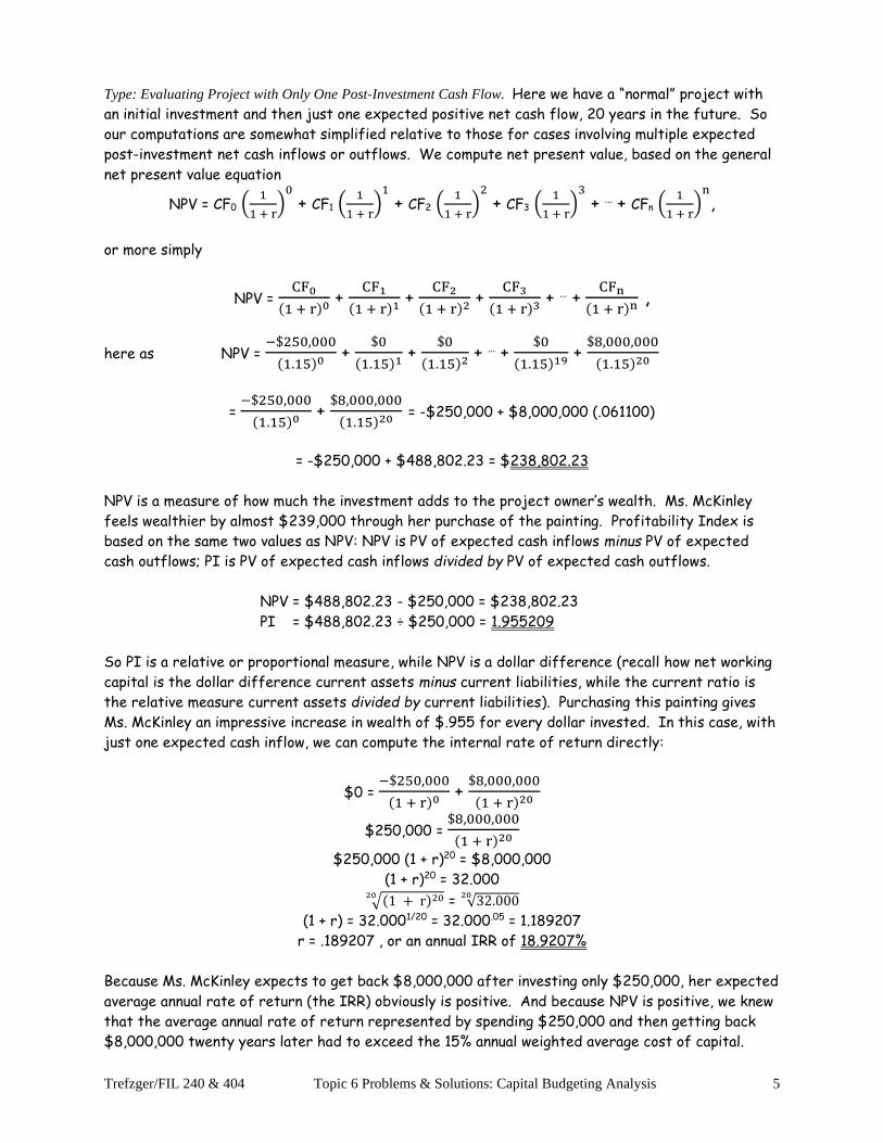
Type: Evaluating Project with Only One Post-Investment Cash Flow. Here we have a “normal” project with
an initial investment and then just one expected positive net cash flow, 20 years in the future. So
our computations are somewhat simplified relative to those for cases involving multiple expected
post-investment net cash inflows or outflows. We compute net present value, based on the general
net present value equation
NPV = CF0 (1
1 + r)
0
+ CF1 (1
1 + r)
1
+ CF2 (1
1 + r)
2
+ CF3 (1
1 + r)
3
+ … + CFn (1
1 + r)
n
,
or more simply
NPV = CF0
(1 + r)0 +
CF1
(1 + r)1 +
CF2
(1 + r)2 +
CF3
(1 + r)3 + … +
CFn
(1 + r)n ,
here as NPV = −$250,000
(1.15)0 +
$0
(1.15)1 +
$0
(1.15)2 + … +
$0
(1.15)19 +
$8,000,000
(1.15)20
= −$250,000
(1.15)0 +
$8,000,000
(1.15)20 = -$250,000 + $8,000,000 (.061100)
= -$250,000 + $488,802.23 = $238,802.23
NPV is a measure of how much the investment adds to the project owner’s wealth. Ms. McKinley
feels wealthier by almost $239,000 through her purchase of the painting. Profitability Index is
based on the same two values as NPV: NPV is PV of expected cash inflows minus PV of expected
cash outflows; PI is PV of expected cash inflows divided by PV of expected cash outflows.
NPV = $488,802.23 - $250,000 = $238,802.23
PI = $488,802.23 ÷ $250,000 = 1.955209
So PI is a relative or proportional measure, while NPV is a dollar difference (recall how net working
capital is the dollar difference current assets minus current liabilities, while the current ratio is
the relative measure current assets divided by current liabilities). Purchasing this painting gives
Ms. McKinley an impressive increase in wealth of $.955 for every dollar invested. In this case, with
just one expected cash inflow, we can compute the internal rate of return directly:
$0 = −$250,000
(1 + r)0 +
$8,000,000
(1 + r)20
$250,000 = $8,000,000
(1 + r)20
$250,000 (1 + r)20 = $8,000,000
(1 + r)20 = 32.000
√(1 + r)2020 = √32.00020
(1 + r) = 32.0001/20 = 32.000.05 = 1.189207
r = .189207 , or an annual IRR of 18.9207%
Because Ms. McKinley expects to get back $8,000,000 after investing only $250,000, her expected
average annual rate of return (the IRR) obviously is positive. And because NPV is positive, we knew
that the average annual rate of return represented by spending $250,000 and then getting back
$8,000,000 twenty years later had to exceed the 15% annual weighted average cost of capital.

Trefzger/FIL 240 & 404 Topic 6 Problems & Solutions: Capital Budgeting Analysis 6
Since there are no intermediate-period cash flows to reinvest, the MIRR – which reflects an
expected reinvesting of cash flows to be received before the investment’s life ends – is the same as
the IRR. (MIRR is a blend of the IRR and the rate earned when the internally generated cash flows
are reinvested in some manner external to the project.) And with no cash expected to be received
until the end of year 20 when the project ends, the payback and discounted payback periods (which
measure how long it takes for the initial investment to be recouped) both are simply 20 years.
3. Everest Steel Fabricating Company plans to pay $4,000,000 for equipment to expand its productive capacity.
The project is expected to generate $800,000 in net cash flows each year of its expected 10-year life. What is the
expected payback period? If the annual weighted average cost of capital for a project such as this one is 12.5%,
what is the expected discounted payback period?
Type: Payback, Discounted Payback. Any “payback” measure predicts how many years it will take for a
capital investment project’s initial investment to be recouped through subsequent net cash flows.
(In our examples we forecast capital investment projects’ cash flows on a total annual basis, since
the uncertainty does not merit using more precise quarterly or monthly figures, although in more
advanced or specialized courses you might see capital budgeting analysis based on quarterly or
monthly cash flow projections.) Payback’s focus is on getting the lenders’ and owners’ money back
fairly quickly, on the logic that unforeseen problems could prevent far distant future expected cash
flows (which would contribute to a higher expected IRR or NPV) from ever actually being received.
When a payback measure is used as an evaluation tool, the project is rejected if it is expected to
take longer than management’s accepted cutoff point to recoup, or pay back, the investment.
A major criticism of payback as a decision criterion is that any such cutoff management chooses is
arbitrary, based on consensus or company history or gut feeling, with no logical or theoretical basis
(why is 3 years the accepted limit, and not 4 or 7 years, for example?). But a defense of payback
is that it stresses the nearer-term future, which managers might feel they have more ability to
foresee. A firm might use a payback measure as a decision tool along with net present value (NPV)
or another more systematic approach; for example, to be accepted a proposed project might have
to have a positive NPV and a measured payback period less than 5 years.
Another criticism of the traditional payback approach (the oldest capital budgeting tool) is that it
treats all future cash flows as being equally valuable, whereas in reality we place greater value on
payments to be received sooner. Using the present values of the expected cash flows in computing
a payback measure allows us to properly penalize cash flows expected to be received farther in the
future. So cash flows we base a payback measure on can be either the stated amounts predicted,
or else their present values. Let’s list both:
“Column 1” “Column 2”
Year Expected Cash Flows 12.5% Present Value Factor PV of Expected Cash Flows
0 ($4,000,000) (1/1.125)0 = 1.0000 ($4,000,000)
1 $800,000 (1/1.125)1 = .8889 $711,111
2 $800,000 (1/1.125)2 = .7901 $632,099
3 $800,000 (1/1.125)3 = .7023 $561,866
4 $800,000 (1/1.125)4 = .6243 $499,436
5 $800,000 (1/1.125)5 = .5549 $443,943
6 $800,000 (1/1.125)6 = .4933 $394,616
7 $800,000 (1/1.125)7 = .4385 $350,770
8 $800,000 (1/1.125)8 = .3897 $311,795

Trefzger/FIL 240 & 404 Topic 6 Problems & Solutions: Capital Budgeting Analysis 7
9 $800,000 (1/1.125)9 = .3464 $277,152
10 $800,000 (1/1.125)10 = .3079 $246,357
Let’s think of the unadjusted cash flow estimates as being “column 1” and their present values,
discounted at the investment project’s 12.5% annual weighted average cost of capital, as being
“column 2.” Our first question is: how many of column 1’s year 1 – 10 positive expected net cash
flows does it take to pay back the $4,000,000 investment? Here we can compute the traditional
“payback period” by keeping a running total in our heads: $800,000 + $800,000 + $800,000 +
$800,000 + $800,000 = $4,000,000 , so it takes 5 of the $800,000 cash flows to pay back the
$4,000,000 investment, and therefore the traditional payback period is 5 years. (If all the
predicted year 1 – n cash flows are the same, we need merely divide year 0’s investment by that
expected annual positive net cash flow: here $4,000,000 ÷ $800,000 = 5.)
Our second question is: how many of column 2’s year 1 – 10 cash flows does it take to pay back the
$4,000,000 year 0 investment, plus fair annual returns to the money providers? We also might
compute this “discounted payback period” by keeping a running total, but can not work the numbers
in our heads because the present values of nice, round $800,000 cash flow estimates are not nice,
round values. But we have a starting point: discounted payback is always longer than traditional
payback (it takes more of the smaller, discounted dollar measures to repay the $4,000,000
investment, or takes longer to pay back the original investment plus appropriate returns to the
money providers than it takes just to pay back the original investment).
So let’s total the first 7 of the positive “column 2” cash flows (the PVs of the cash flows
predicted): $711,111 + $632,099 + $561,866 + $499,436 + $443,943 +$394,616 + $350,770 =
$3,593,841. We have to account for $4,000,000 , so we are not quite there. Add in year 8’s
$311,795 and we are pretty close at $3,905,636. At this stage we are short of the target by only
$4,000,000 – $3,905,636 = $94,364, which is less than the year 9 “column 2” figure. So to pay
back the $4,000,000 investment we need the PVs of the first 8 years’ cash flows, plus $94,364 of
year 9’s $277,152 , for 8 + $94,364/$277,152 = 8.3405 years as the discounted payback period.
A more direct way to compute discounted payback, if the estimated year 1 – n cash flows are equal,
is to set the problem up as a present value of a level ordinary annuity and solve for n:
PMT x FAC = TOT
$800,000 (1−(
1
1.125)
n
.125) = $4,000,000
(1−(
1
1.125)
n
.125) = 5.000
1 − (1
1.125)
n = .625
-(1
1.125)
n = -.375 so (.888889)n = .375
ln [(.888889)n] = ln .375
n (ln .888889) = ln .375
n (– .117783) = – .980829
n = 8.3274 years
Trefzger/FIL 240 & 404 Topic 6 Problems & Solutions: Capital Budgeting Analysis 8
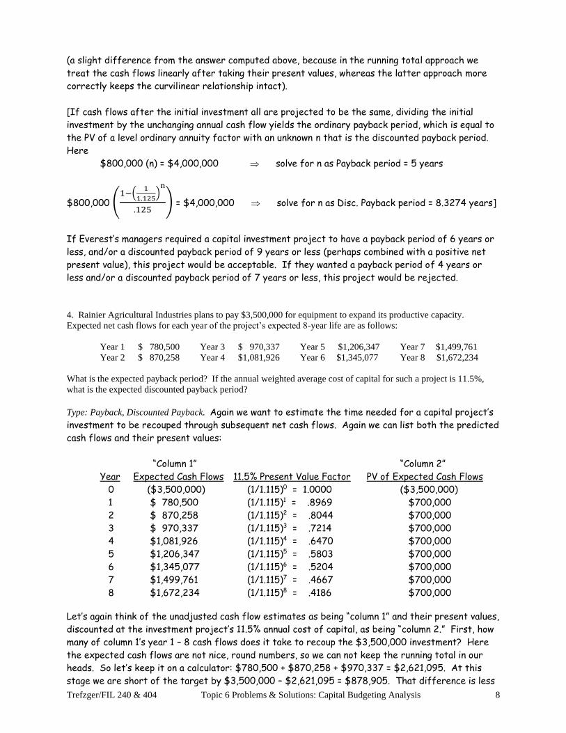
(a slight difference from the answer computed above, because in the running total approach we
treat the cash flows linearly after taking their present values, whereas the latter approach more
correctly keeps the curvilinear relationship intact).
[If cash flows after the initial investment all are projected to be the same, dividing the initial
investment by the unchanging annual cash flow yields the ordinary payback period, which is equal to
the PV of a level ordinary annuity factor with an unknown n that is the discounted payback period.
Here
$800,000 (n) = $4,000,000 solve for n as Payback period = 5 years
$800,000 (1−(
1
1.125)
n
.125) = $4,000,000 solve for n as Disc. Payback period = 8.3274 years]
If Everest’s managers required a capital investment project to have a payback period of 6 years or
less, and/or a discounted payback period of 9 years or less (perhaps combined with a positive net
present value), this project would be acceptable. If they wanted a payback period of 4 years or
less and/or a discounted payback period of 7 years or less, this project would be rejected.
4. Rainier Agricultural Industries plans to pay $3,500,000 for equipment to expand its productive capacity.
Expected net cash flows for each year of the project’s expected 8-year life are as follows:
Year 1 $ 780,500 Year 3 $ 970,337 Year 5 $1,206,347 Year 7 $1,499,761
Year 2 $ 870,258 Year 4 $1,081,926 Year 6 $1,345,077 Year 8 $1,672,234
What is the expected payback period? If the annual weighted average cost of capital for such a project is 11.5%,
what is the expected discounted payback period?
Type: Payback, Discounted Payback. Again we want to estimate the time needed for a capital project’s
investment to be recouped through subsequent net cash flows. Again we can list both the predicted
cash flows and their present values:
“Column 1” “Column 2”
Year Expected Cash Flows 11.5% Present Value Factor PV of Expected Cash Flows
0 ($3,500,000) (1/1.115)0 = 1.0000 ($3,500,000)
1 $ 780,500 (1/1.115)1 = .8969 $700,000
2 $ 870,258 (1/1.115)2 = .8044 $700,000
3 $ 970,337 (1/1.115)3 = .7214 $700,000
4 $1,081,926 (1/1.115)4 = .6470 $700,000
5 $1,206,347 (1/1.115)5 = .5803 $700,000
6 $1,345,077 (1/1.115)6 = .5204 $700,000
7 $1,499,761 (1/1.115)7 = .4667 $700,000
8 $1,672,234 (1/1.115)8 = .4186 $700,000
Let’s again think of the unadjusted cash flow estimates as being “column 1” and their present values,
discounted at the investment project’s 11.5% annual cost of capital, as being “column 2.” First, how
many of column 1’s year 1 – 8 cash flows does it take to recoup the $3,500,000 investment? Here
the expected cash flows are not nice, round numbers, so we can not keep the running total in our
heads. So let’s keep it on a calculator: $780,500 + $870,258 + $970,337 = $2,621,095. At this
stage we are short of the target by $3,500,000 – $2,621,095 = $878,905. That difference is less

Trefzger/FIL 240 & 404 Topic 6 Problems & Solutions: Capital Budgeting Analysis 9
than the year 4 expected cash flow, so we need the first 3 years’ cash flows, plus $878,905 of year
4’s $1,081,926, for a traditional payback period of 3 + $878,905/$1,081,926 = 3.8124 years.
In this (admittedly contrived) example it is the present values of the cash flows that are nice,
round numbers. So in computing the discounted payback period we can keep the running total in our
heads: $700,000 + $700,000 + $700,000 + $700,000 + $700,000 = $3,500,000, so it takes 5 of
the $700,000 present values of expected cash flows to pay back the $3,500,000 investment, and
thus the discounted payback period is 5 years. Here, with the present values of the predicted cash
flows (strangely) equal, we can just divide the $3,500,000 investment by the $700,000 discounted
cash flow per year = 5 years. Note that, as must always be the outcome if the periodic cost of
capital is positive (which it always should be), the discounted payback period is longer than the
traditional payback period. It takes longer to pay the money providers back their money plus a fair
average annual rate of return on their money than it takes merely to pay back their investment.
5. Whitney Specialty Foods, which produces frozen pizzas sold under private brand labels, wants to increase its
manufacturing capacity. Its sales representatives consistently hear from grocery industry executives that a Whitney-
produced frozen lasagna, sold under stores’ own brand names, would create strong consumer interest. As a result,
Whitney’s managers plan to invest $3,200,000 in lasagna processing machinery, which has a 6-year expected life.
The project is expected to create added net cash flows (i.e., beyond what the current money providers get from the
current Whitney business lines) of $650,000 in year 1; $750,000 in year 2; $850,000 in year 3; $950,000 in year 4;
$1,100,000 in year 5; and back to a lower $750,000 in year 6 (as aging equipment and new competition cause
problems). If the annual weighted average cost of capital for a project of this type would be 10.75%, should
Whitney’s managers purchase the new processing machinery? (Include the NPV, PI, IRR, and MIRR criteria.)
Type: Evaluating Expansion Project with Uneven Expected Cash Flows. Our systematic methods for
evaluating a proposed capital investment project are net present value (NPV), profitability index
(PI), internal rate of return (IRR), and modified internal rate of return (MIRR). The general net
present value equation is
NPV = CF0 (1
1 + r)
0
+ CF1 (1
1 + r)
1
+ CF2 (1
1 + r)
2
+ CF3 (1
1 + r)
3
+ … + CFn (1
1 + r)
n
,
or the slightly more convenient version (dividing by a value instead of multiplying by its reciprocal)
NPV = CF0
(1 + r)0 +
CF1
(1 + r)1 +
CF2
(1 + r)2 +
CF3
(1 + r)3 + … +
CFn
(1 + r)n
If the net cash flows for years 1 – n are expected to be equal, we can treat them as an annuity and
save on computational effort. Here, however, net cash flows are expected to differ from year to
year over the project’s expected life, so we must treat each one separately. Thus NPV is computed
as
NPV = -$3,200,000 (1
1.1075)
0
+ $650,000 (1
1.1075)
1
+ $750,000 (1
1.1075)
2
+ $850,000 (1
1.1075)
3
+ $950,000 (1
1.1075)
4
+ $1,100,000 (1
1.1075)
5
+ $750,000 (1
1.1075)
6
= −$3,200,000
(1.1075)0 +
$650,000
(1.1075)1 +
$750,000
(1.1075)2 +
$850,000
(1.1075)3 +
$950,000
(1.1075)4 +
$1,100,000
(1.1075)5 +
$750,000
(1.1075)6
= -$3,200,000 + $586,907 + $611,468 + $625,731 + $631,464 + $660,198 + $406,442
= -$3,200,000 + $3,522,210 = $322,210

Trefzger/FIL 240 & 404 Topic 6 Problems & Solutions: Capital Budgeting Analysis 10
With a positive measured net present value (NPV), the project should be accepted. If Whitney
decides to make frozen lasagna, it expects to be able to pay its workers, material suppliers, power
bills, and other operating costs, along with income taxes, as evidenced by the positive cash flow
projections for years 1 – 6. Recall that cash flow is the money expected to remain, after operating
costs have been covered, for the lenders (in the form of interest) and owners (as dividends and
retained earnings) who pay for the capital equipment. But simply expecting positive net cash flows
does not assure a good investment project; those net cash flows have to be positive enough.
Specifically, they must be enough to repay the lenders’ and owners’ money, plus a fair periodic rate
of return on that money. A $0 NPV indicates that the project will, if expectations prove correct,
provide for the lenders and owners to be repaid, along with a fair rate of return, but with nothing
left over. [In a competitive environment, a $0 NPV – which gives everyone a fair financial return,
though nothing extra – might not be too shabby.] A positive NPV project is expected to provide
for the lenders and owners to be repaid, along with a fair average periodic rate of return, and with
extra money left over (which will belong to the owners, increasing the value of the company they
own, and thus of their common stock, and thus of their wealth). Here a $322,210 NPV means that
if the project is accepted all money providers can expect to be repaid, with fair rates of return in
addition, and the total value of the company’s common stock also should rise by $322,210.
Whereas NPV is the present value of the expected net cash inflows minus the present value of the
net cash outflows (in a simple project, that is the initial investment), profitability index (PI) is the
present value of the expected net cash inflows divided by the PV of the net cash outflows. So here
we have not NPV = $3,522,210 – $3,200,000; but rather PI = $3,522,210 ÷ $3,200,000, or
PI = $3,522,210
$3,200,000 = 1.1007
Profitability index is a relative NPV measure, telling how much NPV is generated per dollar invested.
If NPV is positive, PI is greater than 1.0. Here every dollar invested generates about $.10 in NPV.
IRR is based on the same equation as NPV, but with a different unknown. In NPV analysis we know
the discount rate (the periodic weighted average cost of capital) and must compute the project’s
contribution to the company owners’ wealth. In IRR analysis we set the NPV strategically equal to
$0, and then determine (with trial and error if cash flows are expected to be received in more than
one of the periods beyond year 0) what discount rate makes the equation true. Here we have:
$0 = NPV = −$3,200,000
(1 + r)0 +
$650,000
(1 + r)1 +
$750,000
(1 + r)2 +
$850,000
(1 + r)3 +
$950,000
(1 + r)4 +
$1,100,000
(1 + r)5 +
$750,000
(1 + r)6
With trial and error we would find the rate that solves the equation – the annual IRR – to be
13.9621%; let’s double-check:
−$3,200,000
(1.139621)0 + $650,000
(1.139621)1 + $750,000
(1.139621)2 + $850,000
(1.139621)3 + $950,000
(1.139621)4 + $1,100,000
(1.139621)5 + $750,000
(1.139621)6
= -$3,200,000 + $570,365 + $577,485 + $574,298 + $563,225 + $572,256 + $342,372
= -$3,200,000 + $3,200,000 = $0 ✓
Trefzger/FIL 240 & 404 Topic 6 Problems & Solutions: Capital Budgeting Analysis 11
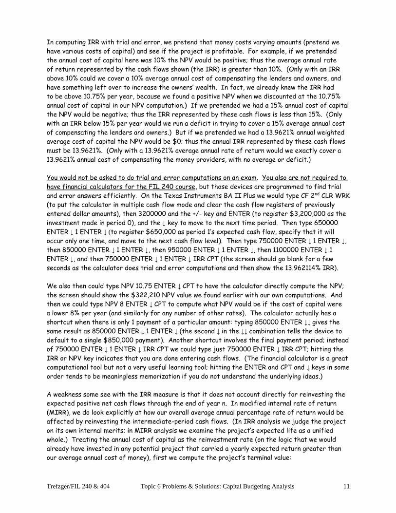
In computing IRR with trial and error, we pretend that money costs varying amounts (pretend we
have various costs of capital) and see if the project is profitable. For example, if we pretended
the annual cost of capital here was 10% the NPV would be positive; thus the average annual rate
of return represented by the cash flows shown (the IRR) is greater than 10%. (Only with an IRR
above 10% could we cover a 10% average annual cost of compensating the lenders and owners, and
have something left over to increase the owners’ wealth. In fact, we already knew the IRR had
to be above 10.75% per year, because we found a positive NPV when we discounted at the 10.75%
annual cost of capital in our NPV computation.) If we pretended we had a 15% annual cost of capital
the NPV would be negative; thus the IRR represented by these cash flows is less than 15%. (Only
with an IRR below 15% per year would we run a deficit in trying to cover a 15% average annual cost
of compensating the lenders and owners.) But if we pretended we had a 13.9621% annual weighted
average cost of capital the NPV would be $0; thus the annual IRR represented by these cash flows
must be 13.9621%. (Only with a 13.9621% average annual rate of return would we exactly cover a
13.9621% annual cost of compensating the money providers, with no overage or deficit.)
You would not be asked to do trial and error computations on an exam. You also are not required to
have financial calculators for the FIL 240 course, but those devices are programmed to find trial
and error answers efficiently. On the Texas Instruments BA II Plus we would type CF 2nd CLR WRK
(to put the calculator in multiple cash flow mode and clear the cash flow registers of previously
entered dollar amounts), then 3200000 and the +/- key and ENTER (to register $3,200,000 as the
investment made in period 0), and the ↓ key to move to the next time period. Then type 650000
ENTER ↓ 1 ENTER ↓ (to register $650,000 as period 1’s expected cash flow, specify that it will
occur only one time, and move to the next cash flow level). Then type 750000 ENTER ↓ 1 ENTER ↓,
then 850000 ENTER ↓ 1 ENTER ↓, then 950000 ENTER ↓ 1 ENTER ↓, then 1100000 ENTER ↓ 1
ENTER ↓, and then 750000 ENTER ↓ 1 ENTER ↓ IRR CPT (the screen should go blank for a few
seconds as the calculator does trial and error computations and then show the 13.962114% IRR).
We also then could type NPV 10.75 ENTER ↓ CPT to have the calculator directly compute the NPV;
the screen should show the $322,210 NPV value we found earlier with our own computations. And
then we could type NPV 8 ENTER ↓ CPT to compute what NPV would be if the cost of capital were
a lower 8% per year (and similarly for any number of other rates). The calculator actually has a
shortcut when there is only 1 payment of a particular amount: typing 850000 ENTER ↓↓ gives the
same result as 850000 ENTER ↓ 1 ENTER ↓ (the second ↓ in the ↓↓ combination tells the device to
default to a single $850,000 payment). Another shortcut involves the final payment period; instead
of 750000 ENTER ↓ 1 ENTER ↓ IRR CPT we could type just 750000 ENTER ↓ IRR CPT; hitting the
IRR or NPV key indicates that you are done entering cash flows. (The financial calculator is a great
computational tool but not a very useful learning tool; hitting the ENTER and CPT and ↓ keys in some
order tends to be meaningless memorization if you do not understand the underlying ideas.)
A weakness some see with the IRR measure is that it does not account directly for reinvesting the
expected positive net cash flows through the end of year n. In modified internal rate of return
(MIRR), we do look explicitly at how our overall average annual percentage rate of return would be
affected by reinvesting the intermediate-period cash flows. (In IRR analysis we judge the project
on its own internal merits; in MIRR analysis we examine the project’s expected life as a unified
whole.) Treating the annual cost of capital as the reinvestment rate (on the logic that we would
already have invested in any potential project that carried a yearly expected return greater than
our average annual cost of money), first we compute the project’s terminal value:

Trefzger/FIL 240 & 404 Topic 6 Problems & Solutions: Capital Budgeting Analysis 12
Year Expected Year-End Cash Flow Reinvestment Factor Terminal Value
1 $ 650,000 (1.1075)5 $1,083,009
2 $ 750,000 (1.1075)4 $1,128,330
3 $ 850,000 (1.1075)3 $1,154,649
4 $ 950,000 (1.1075)2 $1,165,228
5 $1,100,000 (1.1075)1 $1,218,250
6 $ 750,000 (1.1075)0 $ 750,000
Total $6,499,466
If the managers could reinvest each of the year 1 – 6 net cash flows to earn a 10.75% compounded
average annual rate, they would expect to end up, by the end of year 6, with a grand total of
$6,499,466 for the lenders and owners that provided the $3,200,000. (For computational ease or
practicality we treat cash flows as being expected at the end of each year, so by that logic year 1’s
cash flow could be reinvested for 5 years by the end of year 6, while the end-of-year 6 cash flow
could not be reinvested at all.) So a $3,200,000 cash investment is expected to result, 6 years
later, in Whitney’s having $6,499,466 in cash for its money providers. Finding the overall average
periodic return represented by these dollar figures is a simple rate of return problem:
BAMT (1 + r)n = EAMT
$3,200,000 (1 + r)6 = $6,499,466
(1 + r)6 = 2.031083
√(1 + r)66 = √2.0310836
(1 + r) = 2.0310831/6 = 2.031083.166667 = 1.125351
r = .125351 , or an annual MIRR of 12.5351%
MIRR blends the IRR with the assumed reinvestment rate, so its magnitude should be somewhere
between those two values (12.5351% per year is between the 13.9621% annual IRR and the 10.75%
annual weighted average cost of capital).
So, in summary, should the project be accepted? Yes, based on all decision criteria: the NPV is
positive (thus the PI is greater than 1), and the annual IRR and MIRR measures both exceed the
annual cost of capital. Thus the project is expected to create wealth for the company’s owners, by
delivering a rate of return that exceeds the weighted average annual cost of providing fair returns
to the lenders and owners (with the extra, which creates a positive NPV, belonging to the owners).
6. Managers of Eaux Arcs Ice Cream are considering the purchase of new mixing and freezing equipment so they
can produce new flavors and expand their output. The total cost of acquiring the equipment and related items is
expected to be $5,750,000. This type of equipment is expected to have a six-year productive life. Net cash flows
(the money remaining for Eaux Arcs’ lenders and owners, after all operating costs and income taxes have been paid)
are expected to be $1,500,000 in each of years 1 – 6. a. If Eaux Arcs estimates its annual weighted average cost of
capital for an expansion project of this type to be 9.5% per year, should the new ice cream equipment be purchased?
b. What if the annual cost of capital instead were 17%? c. What if the WACC were 14% and a net salvage value of
$1,000,000 could be expected at the end of year 6? (Include the NPV, PI, IRR, and MIRR criteria in your analysis.)
Type: Evaluating Expansion Project with Equal Expected Cash Flows. Again we will evaluate a proposed
capital investment project using the net present value (NPV), profitability index (PI), internal rate
of return (IRR), and modified internal rate of return (MIRR) criteria. And again we can begin with
our general NPV equation:

Trefzger/FIL 240 & 404 Topic 6 Problems & Solutions: Capital Budgeting Analysis 13
NPV = CF0 (1
1 + r)
0
+ CF1 (1
1 + r)
1
+ CF2 (1
1 + r)
2
+ CF3 (1
1 + r)
3
+ … + CFn (1
1 + r)
n
,
although it tends to be easier to compute with the slightly more convenient representation
NPV = CF0
(1 + r)0 +
CF1
(1 + r)1 +
CF2
(1 + r)2 +
CF3
(1 + r)3 + … +
CFn
(1 + r)n
a. If the net cash flows for years 1 – n were expected to differ erratically, we would have to
proceed on a line-by-line, year-by-year basis as we did in the previous problem. And indeed it
is fine to use the same approach even if the year 1 – n cash flows are expected to be equal:
NPV = -$5,750,000 (1
1.095)
0
+ $1,500,000 (1
1.095)
1
+ $1,500,000 (1
1.095)
2
+ $1,500,000 (1
1.095)
3
+ $1,500,000 (1
1.095)
4
+ $1,500,000 (1
1.095)
5
+ $1,500,000 (1
1.095)
6
= −$5,750,000
(1.095)0 +
$1,500,000
(1.095)1 +
$1,500,000
(1.095)2 +
$1,500,000
(1.095)3 +
$1,500,000
(1.095)4 +
$1,500,000
(1.095)5 +
$1,500,000
(1.095)6
= -$5,750,000 + $1,369,863 + $1,251,016 + $1,142,481 + $1,043,361 + $952,841 + $870,175
= -$5,750,000 + $6,629,737 = $879,737
But if we expect net cash flows in a “normal” project all to be the same after the initial investment,
we can compute more quickly by treating the equal amounts as an annuity:
NPV = −$5,750,000
(1.095)0 + $1,500,000 (
1−(1
1.095)
6
.095)
= -$5,750,000 + $1,500,000 (4.419825)
= -$5,750,000 + $6,629,738 = $879,738
(a $1 rounding difference). So it appears that Eaux Arcs should expand its ice cream line. Positive
net cash flow projections show that the firm expects to be able to meet all year 1 – 6 operating
expenses and income tax obligations, and to have $1,500,000 remaining each year for the investors
(lenders and owners) whose money would be used to pay for the $5,750,000 in equipment. But that
alone does not justify going forward; a capital investment project should be accepted only if the
expected cash flows are sufficiently positive to give the investors a return of their money, plus
a fair average periodic rate of return on their investment. Here the weighted average cost of
delivering a fair return to the lenders and owners (the cost of capital) is 9.5% per year. If we
discount the expected net cash flows at a 9.5% annual rate and find a positive NPV, it means the
project is expected to give the investors their money back, plus a fair rate of return (which it costs
the company managers 9.5% yearly to deliver), and also increase the value of the owners’ equity
investment (their common stock) by $879,738. A positive measured NPV, based on the most
careful analysis we can do, therefore tells us to accept the project.
With an NPV computed here as $6,629,738 – $5,750,000 (PV of expected net cash inflows minus
PV of expected net cash outflows), we compute the profitability index as $6,629,738 ÷ $5,750,000:

Trefzger/FIL 240 & 404 Topic 6 Problems & Solutions: Capital Budgeting Analysis 14
PI = $6,629,738
$5,750,000 = 1.1530
Again, with NPV positive the PI is greater than 1.0. Here every dollar invested generates about
$.15 in NPV. In IRR analysis we again set the NPV strategically equal to $0, and use trial and error
to find the discount rate that makes the equation true. Here we have:
$0 = −$5,750,000
(1 + r)0 +
$1,500,000
(1 + r)1 +
$1,500,000
(1 + r)2 +
$1,500,000
(1 + r)3 +
$1,500,000
(1 + r)4 +
$1,500,000
(1 + r)5 +
$1,500,000
(1 + r)6 ,
which can be represented more conveniently as
$0 = −$5,750,000
(1 + r)0 + $1,500,000 (
1−(1
1 + r)
6
r)
With trial and error we would find the rate that solves the equation – the IRR – to be 14.5257%;
let’s double-check:
$0 = −$5,750,000
(1.145257)0 + $1,500,000 (
1−(1
1.145257)
6
.145257)
= -$5,750,000 + $1,500,000 (3.833329)
= -$5,750,000 + $5,750,000 = $0 ✓
In computing IRR with trial and error, we pretend that money costs varying amounts (pretend we
have various annual costs of capital). After presumably trying other cost of capital possibilities,
when we pretend that money costs 14.5257% per year we get an indicated NPV of $0. Only with an
IRR of 14.5257% per year would we exactly cover a 14.5257% annual cost of delivering fair returns
to the money providers, with no overage or deficit. (With the TI BA II Plus financial calculator
we could solve this simple example by entering 5750000 +/- PV, 0 FV, 1500000 PMT, 6 N; CPT I/Y;
the screen would go blank as the device did trial and error computations and then show 14.5257.)
Finally, we could compute the modified internal rate of return as we did with differing year 1 – 6
cash flows. Using the 9.5% annual weighted average cost of capital as an explicit reinvestment rate
(since Eaux Arcs managers already should have invested in any potential project with an expected
average annual return greater than its 9.5% annual cost of money), we proceed as follows:
Year Expected Year-End Cash Flow Reinvestment Factor Terminal Value
1 $1,500,000 (1.095)5 $2,361,358
2 $1,500,000 (1.095)4 $2,156,491
3 $1,500,000 (1.095)3 $1,969,399
4 $1,500,000 (1.095)2 $1,798,538
5 $1,500,000 (1.095)1 $1,642,500
6 $1,500,000 (1.095)0 $1,500,000
Total $11,428,286
But with equal expected year 1 – 6 net cash flows, we can more quickly compute the expected
terminal value by computing the future value of an annuity of $1,500,000 invested at the end
of each year for six years at a 9.5% average annual reinvestment rate:

Trefzger/FIL 240 & 404 Topic 6 Problems & Solutions: Capital Budgeting Analysis 15
PMT x FAC = TOT
$1,500,000 [(1.095)5 + (1.095)4 + (1.095)3 + (1.095)2 + (1.095)1 + (1.095)0] = TOT
$1,500,000 ((1.095)6−1
.095) = TOT
$1,500,000 (7.618857) = $11,428,286
Either way, we see that a $5,750,000 cash investment is expected to result, 6 years later, in the
company managers’ having $11,428,286 in cash for the money providers. Finding the overall average
annual return represented by these dollar figures is a simple rate of return computation:
BAMT (1 + r)n = EAMT
$5,750,000 (1 + r)6 = $11,428,286
(1 + r)6 = 1.987528
√(1 + r)66 = √1.9875286
(1 + r) = 1.9875281/6 = 1.987528.166667 = 1.121293
r = .121293 , or an annual MIRR of 12.1293%
Because MIRR blends the IRR with the assumed periodic reinvestment rate, its 12.1293% annual
magnitude should be somewhere between the 14.5257% yearly IRR and the 9.5% per year cost of
capital (which, in MIRR analysis, we usually treat as the annual reinvestment rate).
Based on all four decision criteria, the project should be accepted if the annual cost of capital is
9.5%. NPV is positive (so of course the PI is greater than 1), and the annual IRR and MIRR measures
both exceed the annual weighted average cost of capital. So the project is expected to create
wealth for the company’s owners, by delivering an average annual rate of return that exceeds the
9.5% annual weighted average cost of providing fair returns to the lenders and owners (with the
extra wealth, in the form of the NPV, belonging to the owners and showing in the form of an
$879,738 increase in the combined value of the existing shares of common stock).
[Textbooks sometimes state that NPV analysis is based on an implicit assumption that cash flows 1
through (n – 1) are reinvested to earn a periodic rate of return equal to the weighted average cost
of capital, while IRR analysis reflects an implicit assumption that cash flows are reinvested to earn
a periodic return equal to the IRR. What such a statement means is that MIRR is equal to IRR, in a
case involving multiple cash flows after the initial investment, only if the reinvestment rate equals
the IRR. Note how the MIRR computation above would change if we used the 14.5257% per year
IRR rather than 9.5% annual cost of capital as the periodic reinvestment rate:
$1,500,000 ((1.145257)6−1
.0145257) = TOT
$1,500,000 (8.649546) = $12,974,319.25; then
$5,750,000 (1 + r)6 = $12,974,319.25
(1 + r)6 = 2.256403 so √(1 + r)66 = √2.2564036
(1 + r) = 2.2564031/6 = 2.256403.166667 = 1.145257; annual MIRR = IRR of 14.5257%]
b. But what if the annual weighted average cost of capital instead were 17%? It is less likely that
a given set of expected net cash flows can return the investors’ money, plus a fair return on that
investment, if the cost of delivering that return (the cost of capital) is higher. Any higher cost –
including the cost of money – leaves a project creating less wealth. For example, NPV now becomes

Trefzger/FIL 240 & 404 Topic 6 Problems & Solutions: Capital Budgeting Analysis 16
NPV = −$5,750,000
(1.17)0 + $1,500,000 (
1−(1
1.17)
6
.17)
= -$5,750,000 + $1,500,000 (3.589185)
= -$5,750,000 + $5,383,777 = -$366,223
If the Eaux Arcs managers committed to doing the project they would cause the total market value
of the company’s existing shares of common stock to decline by $366,223.
While their ability to do trial & error makes financial calculators especially useful in finding IRRs,
we also can use them to solve for NPVs. On the TI BA II Plus we would type CF 2nd CLR WRK (to
put the calculator in cash flow mode and clear the cash flow registers of previously entered dollar
amounts), then 5750000 and the +/- key and ENTER and ↓, then 1500000 and ENTER to register
$1,500,000 as the cash flow expected for the next period and ↓ and 6 and ENTER and ↓ to specify
that the $1,500,000 regular payment is to occur 6 times, then NPV 9.5 ENTER ↓ CPT. The screen
should show the $879,738 net present value based on a 9.5% periodic cost of capital; then NPV 17
ENTER ↓ CPT, the screen should show the -$366,223 NPV based on a 17% periodic cost of capital.
Since the appropriate cash flows all have been entered we also then could type IRR CPT to have the
calculator compute IRR; the screen should go blank briefly while using trial and error to find the
14.5257% internal rate of return we found manually with trial and error earlier. Note that here we
had to type 1500000 ENTER ↓ 6 ENTER ↓ to enter $1,500,000 six times, whereas in earlier problem
5 we could type either 850000 ENTER ↓ 1 ENTER ↓ or the simpler 850000 ENTER ↓↓ to enter
$850,000 one time; the double down arrows ↓↓ tells the calculator to use the default number of
payments of the specified amount, which is 1. (As stated earlier, financial calculators are nice for
computing answers quickly, especially those requiring trial and error. But it is far more important
to know time value of money fundamentals than to memorize sequences of calculator keystrokes.
You are not expected to have a financial calculator for our class, and will never be asked to compute
an IRR for a project with multiple cash flows expected after the initial investment. But you should
be able to write out or identify the equation you would use in solving for such a project’s IRR.)
Eaux Arcs should not expand its ice cream line if the cost of capital is 17% per year; the expected
net cash flows ($1,500,000 x 6 = $9,000,000 total) are not high enough to give the investors their
$5,750,000 back plus provide returns on their remaining investment that cost 17% per year for the
managers to deliver. In fact, taking on this project would reduce the common stockholders’ equity
value by $366,223. A negative NPV tells us not to do the project.
With NPV computed as $5,383,777 – $5,750,000 (PV of expected net cash inflows minus PV of
expected net cash outflows), the profitability index is $5,383,777 ÷ $5,750,000:
PI = $5,383,777
$5,750,000 = .9363
Since NPV is negative the PI is less than 1.0. Here every dollar invested destroys $.0637 in NPV.
IRR is computed based on the expected net cash flows, with no reference to the cost of capital.
We simply view the project as good if the annual IRR (here 14.5257%, as computed earlier based
only on the project’s expected internal cash flows) is greater than the annual weighted average cost

Trefzger/FIL 240 & 404 Topic 6 Problems & Solutions: Capital Budgeting Analysis 17
of capital, bad if the annual cost of capital is greater than the annual IRR. The firm’s managers
certainly could not expect to deliver fair returns to investors at an annual cost of 17% when they
earn only 14.5257% each year on the money those investors provided.
Finally, with a 17% assumed annual reinvestment rate we would compute the modified internal rate
of return as follows:
PMT x FAC = TOT
$1,500,000 [(1.17)5 + (1.17)4 + (1.17)3 + (1.17)2 + (1.17)1 + (1.17)0] = TOT
$1,500,000 ((1.17)6−1
.17) = TOT
$1,500,000 (9.206848) = $13,810,272
is the terminal value, such that a $5,750,000 cash investment is expected to result, 6 years later,
in the company managers’ having $13,810,272 for the lenders and owners that provided the
$5,750,000. The overall average annual rate of return represented by these dollar figures is:
BAMT (1 + r)n = EAMT
$5,750,000 (1 + r)6 = $13,810,272
(1 + r)6 = 2.401786
√(1 + r)66 = √2.4017866
(1 + r) = 2.4017861/6 = 2.401786.166667 = 1.157237
r = .157237 , or an annual MIRR of 15.7237%
MIRR blends the IRR with the assumed reinvestment rate, so here its 15.7237% annual magnitude
should be somewhere between the 14.5257% annual IRR and the 17% annual weighted average cost
of capital. But even if we can accept the logic that we could reinvest at a high 17% average annual
rate, we have to note that the annual MIRR, like the annual IRR, expected from the project is less
than the average annual cost of getting money to invest in the equipment.
Based on all four decision criteria, the project should not be accepted if the annual cost of capital
is 17%. NPV is negative (thus the PI is less than 1), and the cost of capital exceeds both the IRR
and MIRR, so the project is expected to destroy wealth of the company’s owners, by delivering an
annual rate of return less than the 17% weighted average yearly cost of providing fair returns to
the lenders and owners as a group (with the shortfall reducing the owners’ wealth).
c. If Eaux Arcs managers expect to sell the used equipment for $1,000,000 at the end of year 6
(we assume that amount is net of any tax consequences), we could combine that additional expected
year-6 cash flow with the other $1,500,000, or else could leave the group of six $1,500,000 cash
flows as it is and treat the $1,000,000 as a separate amount expected at the end of year 6:
NPV = −$5,750,000
(1.14)0 +
$1,500,000
(1.14)1 +
$1,500,000
(1.14)2 +
$1,500,000
(1.14)3 +
$1,500,000
(1.14)4 +
$1,500,000
(1.14)5 +
$2,500,000
(1.14)6
OR −$5,750,000
(1.14)0 + $1,500,000 (
1−(1
1.14)
5
.14) + $2,500,000 (
1
1.14)
6
Trefzger/FIL 240 & 404 Topic 6 Problems & Solutions: Capital Budgeting Analysis 18
OR −$5,750,000
(1.14)0 + $1,500,000 (
1−(1
1.14)
6
.14) + $1,000,000 (
1
1.14)
6
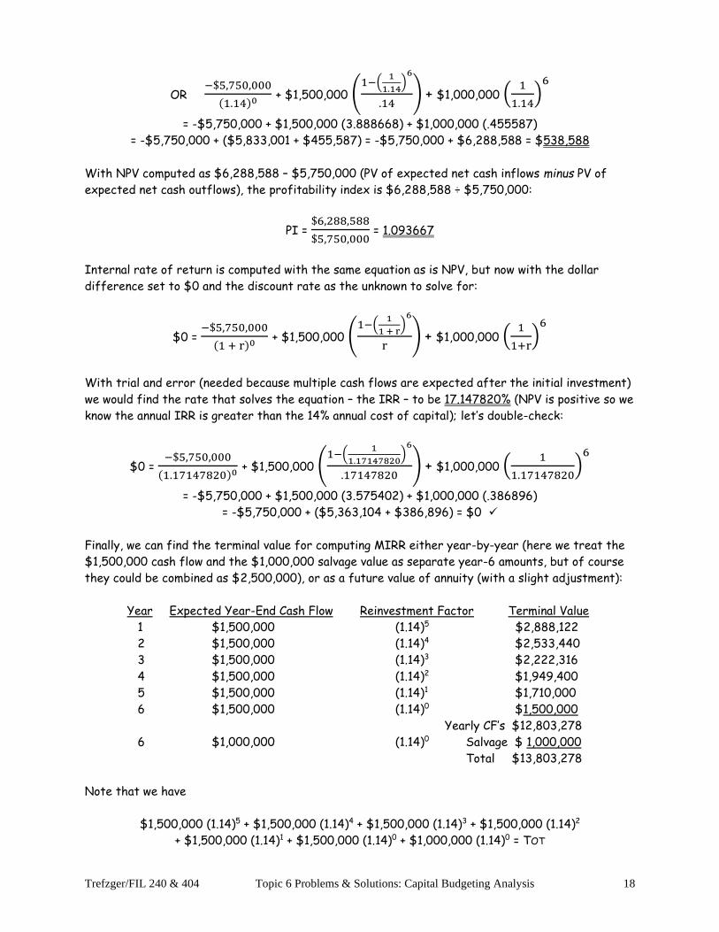
= -$5,750,000 + $1,500,000 (3.888668) + $1,000,000 (.455587)
= -$5,750,000 + ($5,833,001 + $455,587) = -$5,750,000 + $6,288,588 = $538,588
With NPV computed as $6,288,588 – $5,750,000 (PV of expected net cash inflows minus PV of
expected net cash outflows), the profitability index is $6,288,588 ÷ $5,750,000:
PI = $6,288,588
$5,750,000 = 1.093667
Internal rate of return is computed with the same equation as is NPV, but now with the dollar
difference set to $0 and the discount rate as the unknown to solve for:
$0 = −$5,750,000
(1 + r)0 + $1,500,000 (
1−(1
1 + r)
6
r) + $1,000,000 (
1
1+r)
6
With trial and error (needed because multiple cash flows are expected after the initial investment)
we would find the rate that solves the equation – the IRR – to be 17.147820% (NPV is positive so we
know the annual IRR is greater than the 14% annual cost of capital); let’s double-check:
$0 = −$5,750,000
(1.17147820)0 + $1,500,000 (
1−(1
1.17147820)
6
.17147820) + $1,000,000 (
1
1.17147820)
6
= -$5,750,000 + $1,500,000 (3.575402) + $1,000,000 (.386896)
= -$5,750,000 + ($5,363,104 + $386,896) = $0 ✓
Finally, we can find the terminal value for computing MIRR either year-by-year (here we treat the
$1,500,000 cash flow and the $1,000,000 salvage value as separate year-6 amounts, but of course
they could be combined as $2,500,000), or as a future value of annuity (with a slight adjustment):
Year Expected Year-End Cash Flow Reinvestment Factor Terminal Value
1 $1,500,000 (1.14)5 $2,888,122
2 $1,500,000 (1.14)4 $2,533,440
3 $1,500,000 (1.14)3 $2,222,316
4 $1,500,000 (1.14)2 $1,949,400
5 $1,500,000 (1.14)1 $1,710,000
6 $1,500,000 (1.14)0 $1,500,000
Yearly CF’s $12,803,278
6 $1,000,000 (1.14)0 Salvage $ 1,000,000
Total $13,803,278
Note that we have
$1,500,000 (1.14)5 + $1,500,000 (1.14)4 + $1,500,000 (1.14)3 + $1,500,000 (1.14)2
+ $1,500,000 (1.14)1 + $1,500,000 (1.14)0 + $1,000,000 (1.14)0 = TOT

Trefzger/FIL 240 & 404 Topic 6 Problems & Solutions: Capital Budgeting Analysis 19
or, using the distributive property and grouping the unchanging $1,500,000 amounts with the future
value of annuity factor:
$1,500,000 ((1.14)6−1
.14) + $1,000,000 (1.14)0 = Total
$1,500,000 (8.535519) + $1,000,000 (1.00) = $12,803,278 + $1,000,000 = $13,803,278
(or just compute the $1,500,000 (8.535519) = $12,803,278 future value of annuity value and add
the $1,000,000 salvage value to get the combined $13,803,278 terminal value).
So the slight adjustment needed, relative to parts a and b above, is adding the $1,000,000 salvage
value anticipated at the end of year 6 to year 6’s final $1,500,000 regular expected cash flow.
(Since salvage comes at the end of the project’s life there is no opportunity to reinvest between
the date received and the end of the project’s life, so the amount added to the annuity total is just
the unadjusted $1,000,000 salvage value.) The MIRR is found as
BAMT (1 + r)n = EAMT
$5,750,000 (1 + r)6 = $13,803,278
(1 + r)6 = 2.400570
√(1 + r)66 = √2.4005706
(1 + r) = 2.4005701/6 = 2.400570.166667 = 1.157140
r = .157140 , or an annual MIRR of 15.7140%
(again falling somewhere between the 17.15% IRR and the 14% presumed reinvestment rate). Part
c was included in this problem as a preview of computations we will do in the Topic 10 coverage of
bonds. Here for NPV and IRR we combined the present value of an annuity (the equal annual cash
flows) with the present value of a single dollar amount (the anticipated salvage value); in computing
a bond’s value (NPV) or its “yield to maturity” (IRR) we combine the present value of an annuity
(the stream of equal “coupon” interest payments) with the present value of a single dollar amount
(the principal returned at maturity). In computing the MIRR here we had to include the expected
salvage value as part of the terminal value; in computing a bond’s “realized compound yield” (MIRR)
we will have to include the return of the principal at maturity as part of the terminal value; we do
that by adding the par value to the future value of annuity consisting of the reinvested interest
receipts. We may want to refer back to this example during our Topic 10 coverage.
7. Kilimanjaro Manufacturing needs to update its technological equipment. Improved technology is not expected to
bring about higher sales (customers do not care how modern the factory is if the output is of acceptable price and
quality), but would create financial benefits by reducing operating costs. Specifically, if $22,000,000 were invested
in a new company-wide computer network, the firm would expect to realize increased cash flows (through better
hardware compatibility, fewer repair outlays, and reduced general information management costs) of $6 million per
year for 5 years. If Kilimanjaro feels that the cost of capital for a low-risk replacement project of this type is 8.25%
per year, should the new high-tech equipment be purchased? What if the annual cost of capital instead were 16.5%?
Type: Evaluating Replacement Project with Equal Expected Cash Flows. The only conceptual difference
between this question and #6 above is that here the basis for expecting positive net cash flows for
the company’s money providers is cost savings, rather than expanded output. We could compute the
NPV by discounting the five individual year 1 – 5 expected net cash flows:
NPV = −$22,000,000
(1.0825)0 +
$6,000,000
(1.0825)1 +
$6,000,000
(1.0825)2 +
$6,000,000
(1.0825)3 +
$6,000,000
(1.0825)4 +
$6,000,000
(1.0825)5

Trefzger/FIL 240 & 404 Topic 6 Problems & Solutions: Capital Budgeting Analysis 20
But since they are projected to be equal we can save computational time and effort by grouping
them as an annuity:
NPV = −$22,000,000
(1.0825)0 + $6,000,000 (
1−(1
1.0825)
5
.0825)
= -$22,000,000 + $6,000,000 (3.966540)
= -$22,000,000 + $23,799,237 = $1,799,237
(or on the BA II Plus we could enter CF 2nd CLR WRK 22000000 +/- ENTER ↓, 6000000 ENTER ↓ 5
ENTER ↓, NPV 8.25 ENTER ↓ CPT; the screen should show the $1,799,237 net present value). The
net cash flows are expected to be high enough to give the investors their $22,000,000 back plus
returns on their remaining investment that cost the company managers 8.25% per year to deliver,
plus something extra to increase the value of the owners’ common stock, so Kilimanjaro should go
ahead with the project. (Even a $0 NPV would be minimally acceptable, as it would allow all involved
parties – the workers, material suppliers, service providers, tax authorities, and money providers –
to receive fair financial returns, even though if NPV were $0 the value of the firm’s common stock
would be expected to remain the same rather than to increase.)
With NPV computed as PV of expected net cash inflows minus PV of expected net cash outflows
($23,799,237 – $22,000,000), the profitability index is PV of expected net cash inflows divided by
PV of expected net cash outflows ($23,799,237 ÷ $22,000,000):
PI = $23,799,237
$22,000,000 = 1.081784
With NPV positive the PI exceeds 1.0; here every dollar invested leads to about $1.081784 – $1.00
= $.08 in NPV, or wealth for the company’s owners.
In IRR analysis we set the NPV strategically equal to $0, and use trial and error to find the
discount rate that makes the equation true. Here we have:
$0 = −$22,000,000
(1 + r)0 + $6,000,000 (
1−(1
1 + r)
5
r)
With trial and error we would find the annual IRR rate that solves the equation to be 11.3164%;
let’s double-check:
NPV = −$22,000,000
(1.113164)0 + $6,000,000 (
1−(1
1.113164)
5
.113164)
= -$22,000,000 + $6,000,000 (3.666667)
= -$22,000,000 + $22,000,000 = $0 ✓
In computing IRR with trial and error, we pretend that money costs varying amounts (pretend we
have various costs of capital). After presumably trying other periodic weighted average cost of
capital possibilities, when we pretend that money costs 11.3164% per year we get an indicated NPV
of $0. The investment project would exactly cover the cost of providing fair returns to the money
providers, with no overage or deficit, only if that cost were 11.3164% per year, so the average
annual rate of return the project generates must be an IRR of 11.3164%. If all the values remain

Trefzger/FIL 240 & 404 Topic 6 Problems & Solutions: Capital Budgeting Analysis 21
entered in the BA II Plus from the NPV computation above, we can simply hit IRR CPT, and the
screen will go blank for a couple of seconds while the calculator tries and errs and comes up with
the 11.3164% periodic IRR (here it is an annual IRR because of the yearly frequency of the cash
flows). Or, since the year 1 – n cash flows are expected to be equal, we can just enter 22000000
and the +/- key and PV; 0 FV; 6000000 PMT; 5 N; CPT (compute) I/Y; the screen should go blank
briefly and then show 11.3164.
Finally, with an 8.25% assumed annual reinvestment rate we would compute the modified internal
rate of return (MIRR) as follows: the terminal value is projected to be
PMT x FAC = TOT
$6,000,000 ((1.0825)5−1
.0825) = TOT
$6,000,000 (5.895916) = $35,375,498
such that a $22,000,000 cash investment is expected to result, 5 years later, in Kilimanjaro’s
managers having $35,375,498 for the lenders and owners who contributed the $22,000,000.
The overall compounded average annual rate of return represented by these dollar figures is:
BAMT (1 + r)n = EAMT
$22,000,000 (1 + r)5 = $35,375,498
(1 + r)5 = 1.607977
√(1 + r)55 = √1.607977
5
(1 + r) = 1.6079771/5 = 1.607977.2 = 1.099654
r = .099654 , or an annual MIRR of 9.9654%
MIRR blends the IRR with the assumed reinvestment rate; note that the 9.9654% annual MIRR lies
somewhere between the 11.3164% annual IRR and 8.25% per year cost of capital/reinvestment rate.
Based on all four decision criteria, the project should be accepted if the annual cost of capital is
8.25%. NPV is positive (and the PI is greater than 1), and both the annual IRR and MIRR measures
exceed the annual cost of capital. The project is expected to enhance the wealth of the company’s
owners by $1,799,237 (in addition to giving the lenders and owners back their $22 million plus a fair
return on their investment, which here we assume it costs the managers 8.25% annually to deliver).
If the cost of capital were 16.5% per year, however, the project would not provide a positive NPV:
NPV = −$22,000,000
(1.165)0 + $6,000,000 (
1−(1
1.165)
5
.165)
= -$22,000,000 + $6,000,000 (3.236465)
= -$22,000,000 + $19,418,788 = -$2,581,212
(or on the BA II Plus enter CF 2nd CLR WRK 22000000 +/- ENTER ↓, 6000000 ENTER ↓ 5 ENTER ↓,
NPV 16.5 ENTER ↓ CPT; the screen should show the -$2,581,212 net present value). Kilimanjaro
should not upgrade if the annual weighted average cost of capital is 16.5%; expected net cash flows
($6,000,000 x 5 = $30,000,000 total) are not high enough to give the investors their $22,000,000
back, plus returns from year to year on their remaining investment that cost the managers 16.5%
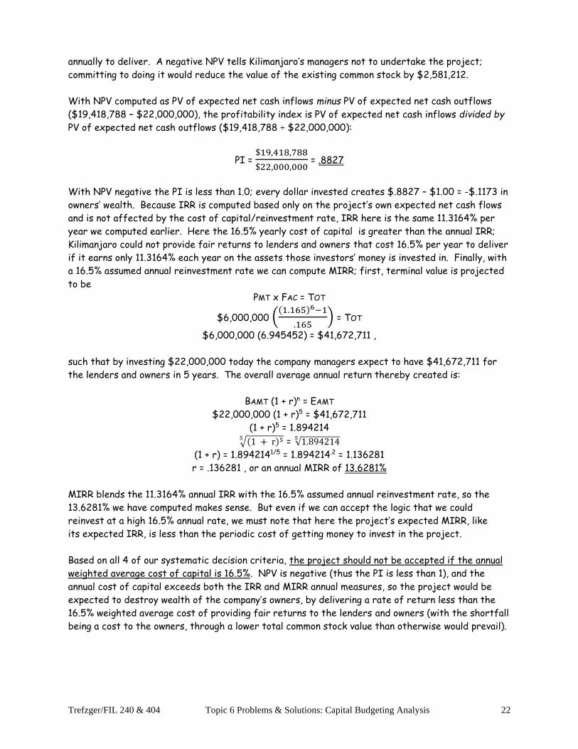
Trefzger/FIL 240 & 404 Topic 6 Problems & Solutions: Capital Budgeting Analysis 22
annually to deliver. A negative NPV tells Kilimanjaro’s managers not to undertake the project;
committing to doing it would reduce the value of the existing common stock by $2,581,212.
With NPV computed as PV of expected net cash inflows minus PV of expected net cash outflows
($19,418,788 – $22,000,000), the profitability index is PV of expected net cash inflows divided by
PV of expected net cash outflows ($19,418,788 ÷ $22,000,000):
PI = $19,418,788
$22,000,000 = .8827
With NPV negative the PI is less than 1.0; every dollar invested creates $.8827 – $1.00 = -$.1173 in
owners’ wealth. Because IRR is computed based only on the project’s own expected net cash flows
and is not affected by the cost of capital/reinvestment rate, IRR here is the same 11.3164% per
year we computed earlier. Here the 16.5% yearly cost of capital is greater than the annual IRR;
Kilimanjaro could not provide fair returns to lenders and owners that cost 16.5% per year to deliver
if it earns only 11.3164% each year on the assets those investors’ money is invested in. Finally, with
a 16.5% assumed annual reinvestment rate we can compute MIRR; first, terminal value is projected
to be
PMT x FAC = TOT
$6,000,000 ((1.165)6−1
.165) = TOT
$6,000,000 (6.945452) = $41,672,711 ,
such that by investing $22,000,000 today the company managers expect to have $41,672,711 for
the lenders and owners in 5 years. The overall average annual return thereby created is:
BAMT (1 + r)n = EAMT
$22,000,000 (1 + r)5 = $41,672,711
(1 + r)5 = 1.894214
√(1 + r)55 = √1.894214
5
(1 + r) = 1.8942141/5 = 1.894214.2 = 1.136281
r = .136281 , or an annual MIRR of 13.6281%
MIRR blends the 11.3164% annual IRR with the 16.5% assumed annual reinvestment rate, so the
13.6281% we have computed makes sense. But even if we can accept the logic that we could
reinvest at a high 16.5% annual rate, we must note that here the project’s expected MIRR, like
its expected IRR, is less than the periodic cost of getting money to invest in the project.
Based on all 4 of our systematic decision criteria, the project should not be accepted if the annual
weighted average cost of capital is 16.5%. NPV is negative (thus the PI is less than 1), and the
annual cost of capital exceeds both the IRR and MIRR annual measures, so the project would be
expected to destroy wealth of the company’s owners, by delivering a rate of return less than the
16.5% weighted average cost of providing fair returns to the lenders and owners (with the shortfall
being a cost to the owners, through a lower total common stock value than otherwise would prevail).

Trefzger/FIL 240 & 404 Topic 6 Problems & Solutions: Capital Budgeting Analysis 23
8. Vesuvius Airways is seeking a long-term supplier for air-sickness “barf” bags. It wants to buy 12 million bags
per year in cases of 600, with each case containing 200 high quality bags (heavy plastic liner, for use in first class),
300 medium quality (thin plastic liner, for use in coach), and 100 low quality (no plastic liner, for college student
fares). The airline is seeking bids from potential suppliers; and will sign a 9-year contract to buy from whichever
supplier submits the lowest bid (i.e., offers to sell for the lowest price). Pike’s Peak Paper Products, which has not
made air-sickness bags in the past, wants to win the Vesuvius account. If Pike’s Peak bought specialized bag-
making machinery with a 9-year expected life, it would cost $4,500,000. Expected material, labor, and other cash-
based variable production costs would be $.05 per bag for the bare-bones model that Pike’s Peak will call the Hurl
Holder, $.10 per bag for its mid-quality Vomit Vault, and $.14 per bag for the top-of-the-line Cookie Catcher. If
Pike’s Peak attributes a 13.75% annual weighted average cost of capital to a project of this type, and if we ignore
income tax effects, for what price should Pike’s Peak bid to sell its 600-bag “Puke-Pak”?
Type: Computing a Bid Price. This problem demonstrates another application of net present value:
determining the price to bid. Under competitive bidding, if a firm’s asking price is too high it loses
the contract to a competitor, while if it bids too low a price it wins the contract but loses money by
failing to cover all costs. An NPV of $0 indicates that the cash flows will be just enough to cover
all expected costs, including a fair rate of return to the firm’s money providers (which includes a
fair “net income” or “accounting profit” for the company’s owners), but nothing more (there would
be no “economic profit”). Indeed, in a competitive environment we would not expect that a business
could do more than cover its costs, including a fair, risk-based, competitive financial return to the
owners.
Because we expect the net cash flows to be the same in each of the 9 years, our general NPV
equation
NPV = CFo
(1 + r)0 +
CF1
(1 + r)1 +
CF2
(1 + r)2 +
CF3
(1 + r)3 + … +
CFn
(1 + r)n ,
can be represented as
NPV = CFo
(1 + r)0 + CF1-n (
1−(1
1 + r)
n
r)
Plugging in the specific values given, we find:
NPV = −$4,500,000
(1.1375)0 + CF1-9 (
1−(1
1.1375)
9
.1375) = $0
-$4,500,000 + CF1 – 9 (4.991678) = $0
$4,500,000 = CF1 – 9 (4.991678)
CF1 – 9 = $901,500
Thus $901,500 is the amount of cash that should remain for the company’s money providers in each
of years 1 – 9, after all other costs have been met, to generate a $0 NPV. How do we begin with
total expected revenues and reach a $901,500 net cash flow level? First consider the expected
cash-based production costs. The average per-bag cost for labor, materials, etc. (a weighted
average, since Pike’s Peak will not make equal numbers of each type) is [100/600 ($.05) + 300/600
($.10) + 200/600 ($.14)] = $.105, or 10.5 cents per bag. With 600 bags in a pack, that totals to
$.105 x 600 = $63 per case for labor, materials, and other per-Puke-Pak variable costs. [We cover
the fixed cost, which presumably consists of having the machinery in place and being used up, by
discounting to a $0 NPV that covers what is to be paid for the machinery.]

Trefzger/FIL 240 & 404 Topic 6 Problems & Solutions: Capital Budgeting Analysis 24
If it will produce 12,000,000 ÷ 600 = 20,000 cases per year, then (ignoring income tax issues) we
can solve for price P as:
20,000 P – 20,000 ($63) = $901,500
20,000 P – $1,260,000 = $901,500
20,000 P = $2,161,500
P = $108.08
It appears that Pikes Peak would want to bid a price of $108.08 per 600-bag Puke-Pak. Of course,
in this analysis we ignored income taxes, the intent being to keep the main ideas simpler to follow.
But by ignoring income tax, which is a significant cost, we actually have computed a price too low
to truly cover all expected costs. If the company were in a 34% marginal income tax bracket, and
wanted (correctly) to charge a price that would cover income tax in addition to all other expected
costs, we could estimate the price it would want to bid to sell each 600-bag Puke-Pak as:
[20,000 P – 20,000 ($63)] (1 – .34) = $901,500
(20,000 P – $1,260,000) (.66) = $901,500
20,000 P (.66) – $831,600 = $901,500
13,200 P = $1,733,100
P = $131.30
9. Fuji Pet Foods is considering two different capital investment projects. One possibility is to make a new product
that would be called Tapir Twinkies; another is to make a new product to be called Muskrat Munchies. Because the
new activity will be handled in a small empty section of Fuji’s current production facility, only one of the projects
can be undertaken. Equipment for either would have a 5-year expected life and a cost of $675,000. Expected net
cash flows (money left for Fuji’s lenders and owners after operating costs and income taxes have been paid) are:
Year Tapir Twinkies Muskrat Munchies
0 ($675,000) ($675,000)
1 $230,000 $180,000
2 $220,000 $190,000
3 $210,000 $200,000
4 $200,000 $210,000
5 $190,000 $220,000
(Fuji analysts expect tapirs to become less popular as pets, while they expect muskrats to grow in popularity,
over the next few years.) Fuji uses a 14% annual cost of capital assumption in evaluating all potential pet food
projects. Compute the net present value (NPV) and modified internal rate of return (MIRR) for each project, and
determine which of the two should be accepted. Should the superior project’s identity actually be readily apparent?
Type: Evaluating Two Equal-Sized Investments. Because net cash flows are expected to differ from year
to year for each project, we can not use the distributive property/annuity shortcut to facilitate
computations. We compute the net present value for each project working year-by-year through
the general NPV equation:
NPV = CFo
(1 + r)0 +
CF1
(1 + r)1 +
CF2
(1 + r)2 +
CF3
(1 + r)3 + … +
CFn
(1 + r)n
For Tapir Twinkies, we compute
NPVTapir Twinkies = −$675,000
(1.14)0 +
$230,000
(1.14)1 +
$220,000
(1.14)2 +
$210,000
(1.14)3 +
$200,000
(1.14)4 +
$190,000
(1.14)5

Trefzger/FIL 240 & 404 Topic 6 Problems & Solutions: Capital Budgeting Analysis 25
= -$675,000 + $201,754 + $169,283 + $141,744 + $118,416 + $98,680
= -$675,000 + $729,877 = $54,877
You are not required to have a financial calculator for our class, and in fact are discouraged from
using such a device’s automated functions until you truly understand what those functions are doing.
But just to show how the sequence of key steps works: on the BA II Plus calculator, type CF 2nd CLR
WRK 675000 and the +/- key and ENTER; that clears any values entered in previous problems done
and registers $675,000 as the investment made in period 0. Then hit the ↓ key and 230000 and
ENTER to register $230,000 as the cash flow expected for period 1, and hit the ↓ key twice (the
first time indicates that the $230,000 occurs only once and the second time moves the process
to the next cash flow level). Then type 220000 ENTER ↓↓, then 210000 ENTER ↓↓, then 200000
ENTER ↓↓, and then 190000 ENTER ↓ NPV 14 ENTER ↓ CPT (it should show the NPV of $54,877.36)
and then go ahead and hit IRR CPT (it should go blank briefly to do trial and error computations
and then show the IRR of 17.45306%, a value we were not asked to compute but with the financial
calculator it is easy enough to find when the cash flow figures already have been entered.)
For Muskrat Munchies, we compute
NPVMuskrat Munchies = −$675,000
(1.14)0 +
$180,000
(1.14)1 +
$190,000
(1.14)2 +
$200,000
(1.14)3 +
$210,000
(1.14)4 +
$220,000
(1.14)5
= -$675,000 + $157,895 + $146,199 + $134,994 + $124,337 + $114,261
= -$675,000 + $677,686 = $2,686
(On the BA II Plus: type CF 2nd CLR WRK 675000 +/- and ENTER and ↓, then 180000 and ENTER
and ↓↓, then 190000 ENTER ↓↓, then 200000 ENTER ↓↓, then 210000 ENTER ↓↓, and then 220000
ENTER ↓ NPV 14 ENTER ↓ CPT (should show the NPV of $2,685.83) and then IRR CPT (should go
blank momentarily and then show the 14.15965% IRR.)
Each project has positive NPV, so each would be accepted if judged on a stand-alone basis. Indeed,
if these projects were “independent” – such that Fuji could conceivably take on both – then the
company would want to make both pet foods, because making each would contribute to the owners’
wealth (although the Muskrat Munchies project would be expected to add only $2,686 to the total
value of Fuji’s common stock, while the Tapir Twinkies project would be expected to raise the
common stock’s total value by $54,877). But in this case the two possible projects are “mutually
exclusive,” meaning that doing one effectively prevents the company from doing the other. So
Tapir Twinkies, with the higher NPV, is the project we would select if NPV were our decision tool.
To compute the modified internal rate of return (MIRR) for Tapir Twinkies, first find the terminal
value to which the reinvested net cash flows would be expected to grow by the end of year 5:
Year Expected Year-End Cash Flow Reinvestment Factor Terminal Value
1 $230,000 (1.14)4 $388,461
2 $220,000 (1.14)3 $325,940
3 $210,000 (1.14)2 $272,916
4 $200,000 (1.14)1 $228,000
5 $190,000 (1.14)0 $190,000
Total $1,405,317

Trefzger/FIL 240 & 404 Topic 6 Problems & Solutions: Capital Budgeting Analysis 26
If each of the year 1 – 5 net cash flows could be reinvested to earn 14% annually, Fuji would expect
to end up with $1,405,317 for the money providers by the end of year 5. So a $675,000 cash
investment is expected to result, 5 years later, in the company managers’ having $1,405,317 in cash
for the lenders and owners that provided the $675,000. The overall annualized return represented
by these dollar figures is computed as:
BAMT (1 + r)n = EAMT
$675,000 (1 + r)5 = $1,405,317
(1 + r)5 = 2.081951
√(1 + r)55 = √2.081951
5
(1 + r) = 2.0819511/5 = 2.081951.2 = 1.157961
r = .157961 , or an annual MIRRTapir Twinkies of 15.7961%
The MIRR for Muskrat Munchies is computed as follows; first compute the terminal value:
Year Expected Year-End Cash Flow Reinvestment Factor Terminal Value
1 $180,000 (1.14)4 $304,013
2 $190,000 (1.14)3 $281,493
3 $200,000 (1.14)2 $259,920
4 $210,000 (1.14)1 $239,400
5 $220,000 (1.14)0 $220,000
Total $1,304,826
With a $675,000 cash investment expected to result, 5 years later, in Fuji’s managers having
$1,304,826 in cash for the lenders and owners who put up the $675,000, we compute the overall
average annual rate of return represented by these dollar figures as:
BAMT (1 + r)n = EAMT
$675,000 (1 + r)5 = $1,304,826
(1 + r)5 = 1.933075
√(1 + r)55 = √1.933075
5
(1 + r) = 1.9330751/5 = 1.933075.2 = 1.140906
r = .140906 , or an annual MIRRMuskrat Munchies of 14.0906%
Because this problem involves two “mutually exclusive” projects, Fuji would want to produce Tapir
Twinkies, with the higher MIRR, if MIRR were its decision tool (as we found using NPV also).
Thus while making Muskrat Munchies would be an acceptable project on a stand-alone basis, in that
its measured NPV is positive and its measured annual MIRR is slightly above the 14% annual cost of
capital, it is not as good a project as Tapir Twinkies when measured either on an NPV standard or
on an MIRR standard; Tapir Twinkies has the higher NPV and the higher MIRR. (And the BA II
Plus financial calculator computations showed that Tapir Twinkies also has the higher IRR, although
finding the IRR here was not required, and you are not expected to have a financial calculator.)
We actually did not have to do much computing to see that Tapir Twinkies is the superior project.
One feature that can make a project more financially attractive than an equally costly alternative
is if its net cash flows are expected to have a higher overall total (although it can depend on the
discount rate). Another feature that can make a project more attractive than an equally costly
alternative is if it is expected to deliver higher net cash flows in the earlier years (which are more
important from a time value perspective, though again it can depend on the discount rate used).

Trefzger/FIL 240 & 404 Topic 6 Problems & Solutions: Capital Budgeting Analysis 27
But here Tapir Twinkies is better than Muskrat Munchies on both counts: the total of its expected
positive cash flows is greater ($1,050,000 vs. $1,000,000 for Muskrat Munchies), and its larger
cash flows are expected in the earlier years (whereas Muskrat Munchies’ earlier, higher-impact
expected cash flows are the smaller ones). With equal project costs and Tapir Twinkies’ expected
net cash flows better than those of Muskrat Munchies in both size and timing we say that Tapir
Twinkies “dominates” Muskrat Munchies. So Tapir Twinkies has to be judged the better project, no
matter what the periodic cost of capital is (even if it is zero) or what type of decision criterion is
used. (Even a payback measure would favor Tapir Twinkies, with higher cash flows expected in the
early years.) Thus, if the two projects are mutually exclusive, Fuji should pursue the production of
Tapir Twinkies.
10. Grand Teton Building Products wants to manufacture pre-cut shelves to sell in large home improvement stores.
One possibility is to make traditional plywood shelves, for which net cash flows would be expected to start strong
but then decline over time as younger people, who often prefer new synthetic materials, become home owners in
greater numbers. The other approach would be to make shelves out of a laminated plastic material, for which net
cash flows would be expected to start out lower but then rise over time. The equipment for producing either type
of shelving would have a 7-year expected life, and a cost today of $258,000. Net cash flows (money left for Grand
Teton’s lenders and owners, after all operating costs and income taxes have been paid) are expected to be as follows:
Year Plywood Plastic
0 ($258,000) ($258,000)
1 $85,000 $45,000
2 $75,000 $50,000
3 $65,000 $55,000
4 $55,000 $65,000
5 $50,000 $75,000
6 $45,000 $85,000
7 $40,000 $95,000
If the two possibilities are mutually exclusive, such that only one type of shelving would be produced, and if Grand
Teton uses an 8% annual cost of capital assumption in evaluating all potential building materials projects, which
type of shelving should it produce? What if the annual cost of capital instead were 15%? In making your decision,
compute the modified internal rate of return (MIRR) for each project, and compile a brief net present value (NPV)
profile for each project. Why is the identity of the superior project not readily apparent in this example?
Type: Evaluating Two Equal-Sized Investments. Let’s briefly address the last part of the question first.
Here the Plywood project has the advantage of higher expected cash flows in the early years. But
Plastic has the advantage of a higher expected cash flow total over the 7-year expected life that
the projects share. So unlike the situation in earlier problem 9 neither project “dominates” the
other; the preferred choice will depend on the assumption we make regarding the annual weighted
average cost of capital. And again as in problem 9 the net cash flows are expected to differ from
year to year for each project, so we can not use the distributive property/annuity shortcut to
facilitate computations. To find the MIRR for the Plywood shelving project, with an 8% annual cost
of capital, first we compute the terminal value of the reinvested cash flows:
Year Expected Year-End Cash Flow Reinvestment Factor Terminal Value
1 $85,000 (1.08)6 $134,884
2 $75,000 (1.08)5 $110,200
3 $65,000 (1.08)4 $ 88,432
4 $55,000 (1.08)3 $ 69,284
5 $50,000 (1.08)2 $ 58,320
6 $45,000 (1.08)1 $ 48,600

Trefzger/FIL 240 & 404 Topic 6 Problems & Solutions: Capital Budgeting Analysis 28
7 $40,000 (1.08)0 $ 40,000
Total $549,720
If Grand Teton could reinvest the year 1 – 7 net cash flows to earn 8% annually, it would expect to
end up with $549,720 by the end of year 7. So a $258,000 cash investment is expected to result
7 years later in the company managers’ having $549,720 in cash for the lenders and owners who
provided the $258,000, for an overall average annual rate of return computed as:
BAMT (1 + r)n = EAMT
$258,000 (1 + r)7 = $549,720
(1 + r)7 = 2.130698
√(1 + r)77 = √2.1306987
(1 + r) = 2.1306981/7 = 2.130698.142857 = 1.114119
r = .114119 , or annual MIRRPlywood of 11.4119%
The terminal value for the Plastic shelving project, with an 8% annual cost of capital, is
Year Expected Year-End Cash Flow Reinvestment Factor Terminal Value
1 $45,000 (1.08)6 $ 71,409
2 $50,000 (1.08)5 $ 73,466
3 $55,000 (1.08)4 $ 74,827
4 $65,000 (1.08)3 $ 81,881
5 $75,000 (1.08)2 $ 87,480
6 $85,000 (1.08)1 $ 91,800
7 $95,000 (1.08)0 $ 95,000
Total $575,863
With a $258,000 cash investment expected to result in Grand Teton’s having $575,863 in cash
for its lenders and owners 7 years later, the average annual overall rate of return, the MIRR, is:
BAMT (1 + r)n = EAMT
$258,000 (1 + r)7 = $575,863
(1 + r)7 = 2.232027
√(1 + r)77 = √2.2320277
(1 + r) = 2.2320271/7 = 2.232027.142857 = 1.121538
r = .121538 , or an annual MIRRPlastic of 12.1538%
With a fairly low cost of capital, the Plastic shelving project is preferred, as measured by a higher
annual MIRR (if the opportunity cost of waiting is low then the project that ultimately delivers
more dollars is better). But with a higher cost of capital the ranking is reversed; the Plywood
shelving project is preferred (if the opportunity cost of waiting is high then the project that
delivers more dollars sooner is better). Note that at a 15% annual cost of capital the MIRRs are:
Year Expected Year-End Cash Flow Reinvestment Factor Terminal Value
1 $85,000 (1.15)6 $196,610
2 $75,000 (1.15)5 $150,852
3 $65,000 (1.15)4 $113,685
4 $55,000 (1.15)3 $ 83,648
5 $50,000 (1.15)2 $ 66,125

Trefzger/FIL 240 & 404 Topic 6 Problems & Solutions: Capital Budgeting Analysis 29
6 $45,000 (1.15)1 $ 51,750
7 $40,000 (1.15)0 $ 40,000
Total $702,670
BAMT (1 + r)n = EAMT
$258,000 (1 + r)7 = $702,670
(1 + r)7 = 2.723528
√(1 + r)77 = √2.7235287
(1 + r) = 2.7235281/7 = 2.723528.142857 = 1.153883
r = .153883 , or an annual MIRRPlywood of 15.3883%
for the Plywood shelving project, but a lower MIRR for the Plastic shelving project of
Year Expected Year-End Cash Flow Reinvestment Factor Terminal Value
1 $45,000 (1.15)6 $104,088
2 $50,000 (1.15)5 $100,568
3 $55,000 (1.15)4 $ 96,195
4 $65,000 (1.15)3 $ 98,857
5 $75,000 (1.15)2 $ 99,188
6 $85,000 (1.15)1 $ 97,750
7 $95,000 (1.15)0 $ 95,000
Total $691,646
BAMT (1 + r)n = EAMT
$258,000 (1 + r)7 = $691,646
(1 + r)7 = 2.680798
√(1 + r)77 = √2.6807987
(1 + r) = 2.6807981/7 = 2.680798.142857 = 1.151279
r = .151279 , or an annual MIRRPlastic of 15.1279%
Thus under the MIRR criterion the Plastic project is slightly better at an 8% annual cost of money,
but Plywood is slightly better at a 15% annual cost of money. Does net present value show the same
ranking? We compute for each project working year-by-year through the general net present value
equation:
NPV = CF0
(1 + r)0 +
CF1
(1 + r)1 +
CF2
(1 + r)2 +
CF3
(1 + r)3 + … +
CFn
(1 + r)n
For the Plywood shelving, we compute NPV at an 8% annual cost of capital as
NPV = −$258,000
(1.08)0 +
$85,000
(1.08)1 +
$75,000
(1.08)2 +
$65,000
(1.08)3 +
$55,000
(1.08)4 +
$50,000
(1.08)5 +
$45,000
(1.08)6 +
$40,000
(1.08)7
= -$258,000 + $78,704 + $64,300 + $51,599 + $40,427 + $34,029 + $28,358 + $23,340
= -$258,000 + $320,757 = $62,757 NPVPlywood
For the Plastic shelving, at an 8% annual cost of capital we compute
NPV = −$258,000
(1.08)0 +
$45,000
(1.08)1 +
$50,000
(1.08)2 +
$55,000
(1.08)3 +
$65,000
(1.08)4 +
$75,000
(1.08)5 +
$85,000
(1.08)6 +
$95,000
(1.08)7
= -$258,000 + $41,667 + $42,867 + $43,661 + $47,777 + $51,044 + $53,564 + $55,432
= -$258,000 + $336,012 = $78,012 NPVPlastic

Trefzger/FIL 240 & 404 Topic 6 Problems & Solutions: Capital Budgeting Analysis 30
Each project has a positive NPV, and thus each would be expected to generate enough cash to give
the lenders and owners back their $258,000 investment, plus financial returns on their $258,000
investment that cost the managers 8% per year to deliver, plus something extra to increase the
total value of the owners’ common stock. But at an 8% annual cost of capital, making Plastic shelving
contributes more to the owners’ wealth, and thus Grand Teton should select it under the NPV
criterion since the two projects are “mutually exclusive.” So the Plastic shelving project is chosen
under either the MIRR or the NPV criterion, if the annual weighted average cost of capital is 8%.
What if the yearly weighted average cost of capital is 15%? The computed net present values are:
NPV = −$258,000
(1.15)0 +
$85,000
(1.15)1 +
$75,000
(1.15)2 +
$65,000
(1.15)3 +
$55,000
(1.15)4 +
$50,000
(1.15)5 +
$45,000
(1.15)6 +
$40,000
(1.15)7
= -$258,000 + $73,913 + $56,711 + $42,739 + $31,446 + $24,859 + $19,455 + $15,037
= -$258,000 + $264,160 = $6,160 NPVPlywood, and a lower
NPV = −$258,000
(1.15)0 +
$45,000
(1.15)1 +
$50,000
(1.15)2 +
$55,000
(1.15)3 +
$65,000
(1.15)4 +
$75,000
(1.15)5 +
$85,000
(1.15)6 +
$95,000
(1.15)7
= -$258,000 + $39,130 + $37,807 + $36,163 + $37,164 + $37,288 + $36,748 + $35,714
= -$258,000 + $260,014 = $2,014 NPVPlastic
Thus the Plywood shelving project is chosen under either the MIRR or the NPV criterion, if the
annual cost of capital is 15%. So NPV and MIRR give the same rankings under both cost of capital
assumptions. For two normal capital investment projects (negative initial cash flows, positive
expected net cash flows thereafter) with equal sized year 0 investment outlays, the NPV and
IRR or MIRR criteria will always give the same rankings. But recall that here we do not have one
project whose expected net cash flows clearly dominate the other’s, so which project is judged
superior can depend on the periodic discount rate (cost of capital). Plastic shelving offers an
advantage in one general sense: the total expected to be received in years 1 – 7, after $258,000 is
invested in year 0, is higher ($470,000 , vs. $415,000 for Plywood shelves). But Plywood offers a
different general advantage: its bigger cash flows are expected to be received earlier ($85,000 in
year 1, vs. $45,000 for Plastic shelves).
So each project is better on an important dimension: getting more cash is better, but getting cash
sooner also is better. Which project is judged better overall ends up depending on the periodic
cost of getting money from investors. If it is only 8% per year the company feels little pain in
having to wait several years to get the Plastic shelf project’s larger cash flows; after all, money
that remains tied up in the project is fairly cheap (or viewed slightly differently, if the company
collected the money sooner the managers could not invest it to earn more than a fairly low 8% per
year). But at 15% per year, it is very costly to have to wait to get the larger expected inflows, but
not that painful to sacrifice small amounts if they would be received farther off in the future. So
if you had to wait a long time to get money, it would be better if the amount you were waiting for
were small.
In summary, at a higher periodic cost of money both projects are less profitable, in time value-
adjusted terms, than with a lower periodic cost of capital (less is left as an NPV if more must be
taken from the cash flows to provide a higher basic rate of return to the investors). But for an

Trefzger/FIL 240 & 404 Topic 6 Problems & Solutions: Capital Budgeting Analysis 31
annual weighted average cost of capital higher than about 13.16% the Plywood project is better
(where the larger cash flows are discounted at a high periodic rate but not for too many periods),
while for a cost of capital below that figure the Plastic project is better (where the larger cash
flows are discounted for many periods but not at a high periodic rate). [We get this 13.16%
“crossover rate” by computing the IRR for a project whose cash flows are the difference between
the Plywood and Plastic shelving projects’ cash flows; we also could just try different discount rates
until the two projects’ NPVs were the same.]
An “NPV profile” shows net present values based on a range of assumed periodic costs of capital.
Note that at a 0% annual weighted average cost of capital (the lowest we would typically think of
as being possible) the NPVs would be:
NPV = −$258,000
(1.00)0 +
$85,000
(1.00)1 +
$75,000
(1.00)2 +
$65,000
(1.00)3 +
$55,000
(1.00)4 +
$50,000
(1.00)5 +
$45,000
(1.00)6 +
$40,000
(1.00)7
= -$258,000 + $85,000 + $75,000 + $65,000 + $55,000 + $50,000 + $45,000 + $40,000
= -$258,000 + $415,000 = $157,000 for the Plywood shelving project, and a higher
NPV = −$258,000
(1.00)0 +
$45,000
(1.00)1 +
$50,000
(1.00)2 +
$55,000
(1.00)3 +
$65,000
(1.00)4 +
$75,000
(1.00)5 +
$85,000
(1.00)6 +
$95,000
(1.00)7
= -$258,000 + $45,000 + $50,000 + $55,000 + $65,000 + $75,000 + $85,000 + $95,000
= -$258,000 + $470,000 = $212,000 for the Plastic shelving project.
A 0% periodic discount rate gives the highest possible NPV figures. The other extreme is the
infinite periodic cost of capital (the highest that possibly could exist), which gives the lowest
possible NPV for a project. If the annual discount rate is infinitely high, the present value of
any cash flow expected today is its full (negative) unadjusted value, while the PV of any cash flow
expected after today is $0, so the NPVs would be:
NPV = −$258,000
(1 + )0 +
$85,000
(1 + )1 +
$75,000
(1 + )2 +
$65,000
(1 + )3 +
$55,000
(1 + )4 +
$50,000
(1 + )5 +
$45,000
(1 + )6 +
$40,000
(1 + )7
= -$258,000 + $0 + $0 + $0 + $0 + $0 + $0 + $0
= -$258,000 for the Plywood shelving project, and also
NPV = −$258,000
(1 + )0 +
$45,000
(1 + )1 +
$50,000
(1 + )2 +
$55,000
(1 + )3 +
$65,000
(1 + )4 +
$75,000
(1 + )5 +
$85,000
(1 + )6 +
$95,000
(1 + )7
= -$258,000 + $0 + $0 + $0 + $0 + $0 + $0 + $0
= -$258,000 for the Plastic shelving project.
(Thus at an infinite discount rate the project’s NPV is simply the year 0 cash investment.) At a
13.16% annual weighted average cost of capital (crossover point noted above), the NPVs would be:
NPV = −$258,000
(1.1316)0 +
$85,000
(1.1316)1 +
$75,000
(1.1316)2 +
$65,000
(1.1316)3 +
$55,000
(1.1316)4 +
$50,000
(1.1316)5 +
$45,000
(1.1316)6 +
$40,000
(1.1316)7
= -$258,000 + $75,115 + $58,570 + $44,857 + $33,542 + $26,947 + $21,432 + $16,835
= –$258,000 + $277,298 = $19,298 for the Plywood shelving project, and also
NPV = −$258,000
(1.1316)0 +
$45,000
(1.1316)1 +
$50,000
(1.1316)2 +
$55,000
(1.1316)3 +
$65,000
(1.1316)4 +
$75,000
(1.1316)5 +
$85,000
(1.1316)6 +
$95,000
(1.1316)7
= -$258,000 + $39,767 + $39,047 + $37,956 + $39,641 + $40,420 + $40,482 + $39,983
= -$258,000 + $277,296 = $19,296 ($2 rounding difference) for the Plastic shelving project.

Trefzger/FIL 240 & 404 Topic 6 Problems & Solutions: Capital Budgeting Analysis 32
Finally, at a 15.92% annual weighted average cost of capital, the Plywood project’s NPV would be:
NPV = −$258,000
(1.1592)0 +
$85,000
(1.1592)1 +
$75,000
(1.1592)2 +
$65,000
(1.1592)3 +
$55,000
(1.1592)4 +
$50,000
(1.1592)5 +
$45,000
(1.1592)6 +
$40,000
(1.1592)7
= -$258,000 + $73,326 + $55,814 + $41,729 + $30,460 + $23,888 + $18,547 + $14,222
= –$258,000 + $258,000 = $0 (so 15.92%, actually 15.917826%, is the Plywood project’s IRR),
while at a 15.23% annual weighted average cost of capital the Plastic project’s NPV would be:
NPV = −$258,000
(1.1523)0 +
$45,000
(1.1523)1 +
$50,000
(1.1523)2 +
$55,000
(1.1523)3 +
$65,000
(1.1523)4 +
$75,000
(1.1523)5 +
$85,000
(1.1523)6 +
$95,000
(1.1523)7
= -$258,000 + $39,052 + $37,656 + $35,947 + $36,868 + $36,918 + $36,310 + $35,218
= –$258,000 + $258,000 = $0 (so 15.23%, actually 15.226571%, is the Plastic project’s IRR).
Thus we have a range of NPV measures, depending on the assumed periodic weighted average cost
of capital. A brief representation of an NPV profile would be:
Discount Rate Plywood Shelving NPV Plastic Shelving NPV
0% (Plastic higher) $157,000 $212,000
8% (Plastic higher) $62,757 $78,012
13.16% (Crossover) $19,298 $19,298
15% (Plywood higher) $6,160 $2,014
15.23% (Plywood higher) $4,593 $0
15.92% (Plywood higher) $0 -$6,023
Infinite -$258,000 -$258,000
We sometimes think of NPV as a very straightforward idea, but in reality the NPV we compute is
entirely dependent on the cost of capital figure we use – and there could be cases, such as when a
company enters a new line of business, in which it is hard to estimate the returns the company’s
lenders and owners would require. Thus we might like to create an NPV profile. One benefit of
being able to use a financial calculator is that once the cash flows have been entered we can easily
change the discount rate (whatever we assume the cost of capital is) and get a new NPV figure,
toward putting together an NPV profile. For the plywood shelving project, on the BA II Plus we
would type CF 2nd CLR WRK, then 258000 and the +/- key and ENTER. Then hit the ↓ key to move
to the next time period, and type 85000 and hit ENTER and hit the ↓ key twice (to specify the
default condition of a single payment at that level and move to the next period). Then type 75000
ENTER ↓↓, 65000 ENTER ↓↓, 55000 ENTER ↓↓, 50000 ENTER ↓↓, 45000 ENTER ↓↓, and 40000
ENTER ↓ NPV 8 ENTER ↓ CPT; screen should show the $62,756 NPV value we found earlier with our
own computations. Then NPV 15 ENTER ↓ CPT, it should show $6,160; then NPV 0 ENTER ↓ CPT, it
should show $157,000; finally NPV 15.917826 ENTER ↓ CPT, it should show a small amount close to
$0 with a very tiny rounding difference (using the IRR as the discount rate yields a $0 NPV).
11. St. Helens Corporation wants to begin making pens. One possibility is to make low-priced disposables; another
is to make high-end models selling for several hundred dollars each. Because high-end buyers would not purchase
expensive pens from a company also known for cheap throw-aways, it would be impractical to produce both types.
Equipment for producing the low-priced model would cost $450,000 and result in expected net cash flows (money
left for St. Helens’s investors after all operating costs and income taxes had been paid) of $94,500 in each of the 8
years the equipment would be expected to last. Equipment for the high-priced model would cost $685,500, with
expected net cash flows of $142,750 in each of the 8 years of the equipment’s expected life. St. Helens uses an

Trefzger/FIL 240 & 404 Topic 6 Problems & Solutions: Capital Budgeting Analysis 33
11.75% annual cost of capital assumption in evaluating investment projects. Compute the net present value (NPV)
and modified internal rate of return (MIRR) for each project, and determine which one St. Helens should accept.
Type: Evaluating Two Unequal-Sized Investments. Here each potential project’s net cash flows are
expected to be unchanging after the initial investment has been made. Thus we can achieve the
result of the general net present value equation:
NPV = CF0
(1 + r)0 +
CF1
(1 + r)1 +
CF2
(1 + r)2 +
CF3
(1 + r)3 + … +
CFn
(1 + r)n ,
with the more abbreviated format we can use with cash flows 1 through 8 projected to be equal:
NPVLow-Priced = −$450,000
(1.1175)0 + $94,500 (
1−(1
1.1175)
8
.1175)
= -$450,000 + $94,500 (5.011333)
= -$450,000 + $473,571 = $23,571 for the low-priced pen project and
NPVHigh-Priced = −$685,500
(1.1175)0 + $142,750 (
1−(1
1.1175)
8
.1175)
= -$685,500 + $142,750 (5.011333)
= -$685,500 + $715,368 = $29,868 for the high-priced pen project.
Each project has a positive NPV, and thus each would be expected to generate enough cash to give
the lenders and owners back their investment, plus annual returns on their remaining outstanding
investment that cost 11.75% per year to deliver, plus something extra to increase the total value of
the existing shares of the owners’ common stock. But making expensive pens contributes more to
the owners’ wealth than does making cheap ones, and thus the NPV decision tool tells the company
to produce expensive pens. Now let’s consider the two proposed projects’ MIRRs. For the low-
priced pen project we compute a terminal value of
PMT x FAC = TOT
$94,500 ((1.1175)8−1
.1175) = TOT
$94,500 (12.188029) = $1,151,769 Terminal Value
If St. Helens could reinvest the year 1 – 8 net cash flows to earn 11.75% annually, the managers
would expect to have $1,151,769 by the end of year 8. So a $450,000 cash investment is expected
to result in the company’s having $1,151,769 in cash for the lenders and owners 8 years later, for an
overall average annual rate of return computed as:
BAMT (1 + r)n = EAMT
$450,000 (1 + r)8 = $1,151,769
(1 + r)8 = 2.559487
√(1 + r)88 = √2.5594878
(1 + r) = 2.5594871/8 = 2.559487.125 = 1.124654
r = .124654 , or an annual MIRRLow-Priced of 12.4654%
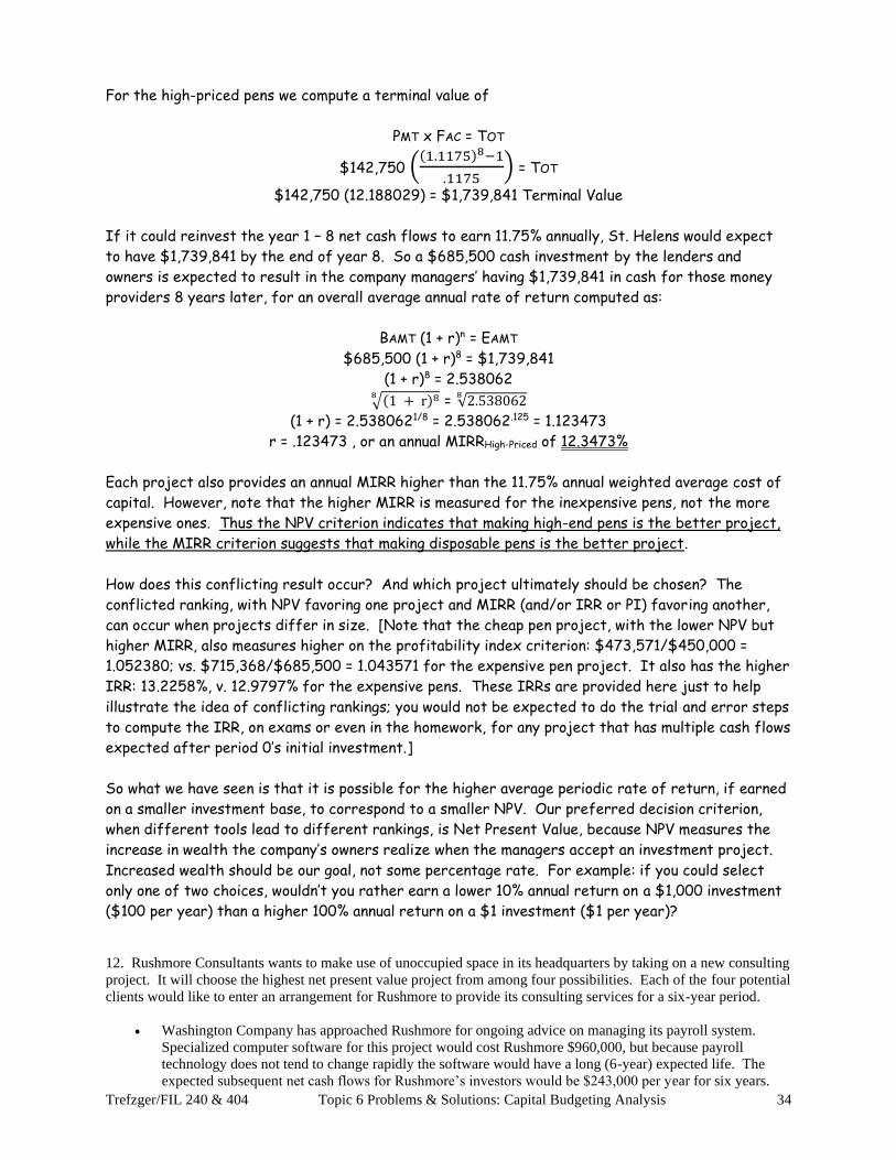
Trefzger/FIL 240 & 404 Topic 6 Problems & Solutions: Capital Budgeting Analysis 34
For the high-priced pens we compute a terminal value of
PMT x FAC = TOT
$142,750 ((1.1175)8−1
.1175) = TOT
$142,750 (12.188029) = $1,739,841 Terminal Value
If it could reinvest the year 1 – 8 net cash flows to earn 11.75% annually, St. Helens would expect
to have $1,739,841 by the end of year 8. So a $685,500 cash investment by the lenders and
owners is expected to result in the company managers’ having $1,739,841 in cash for those money
providers 8 years later, for an overall average annual rate of return computed as:
BAMT (1 + r)n = EAMT
$685,500 (1 + r)8 = $1,739,841
(1 + r)8 = 2.538062
√(1 + r)88 = √2.5380628
(1 + r) = 2.5380621/8 = 2.538062.125 = 1.123473
r = .123473 , or an annual MIRRHigh-Priced of 12.3473%
Each project also provides an annual MIRR higher than the 11.75% annual weighted average cost of
capital. However, note that the higher MIRR is measured for the inexpensive pens, not the more
expensive ones. Thus the NPV criterion indicates that making high-end pens is the better project,
while the MIRR criterion suggests that making disposable pens is the better project.
How does this conflicting result occur? And which project ultimately should be chosen? The
conflicted ranking, with NPV favoring one project and MIRR (and/or IRR or PI) favoring another,
can occur when projects differ in size. [Note that the cheap pen project, with the lower NPV but
higher MIRR, also measures higher on the profitability index criterion: $473,571/$450,000 =
1.052380; vs. $715,368/$685,500 = 1.043571 for the expensive pen project. It also has the higher
IRR: 13.2258%, v. 12.9797% for the expensive pens. These IRRs are provided here just to help
illustrate the idea of conflicting rankings; you would not be expected to do the trial and error steps
to compute the IRR, on exams or even in the homework, for any project that has multiple cash flows
expected after period 0’s initial investment.]
So what we have seen is that it is possible for the higher average periodic rate of return, if earned
on a smaller investment base, to correspond to a smaller NPV. Our preferred decision criterion,
when different tools lead to different rankings, is Net Present Value, because NPV measures the
increase in wealth the company’s owners realize when the managers accept an investment project.
Increased wealth should be our goal, not some percentage rate. For example: if you could select
only one of two choices, wouldn’t you rather earn a lower 10% annual return on a $1,000 investment
($100 per year) than a higher 100% annual return on a $1 investment ($1 per year)?
12. Rushmore Consultants wants to make use of unoccupied space in its headquarters by taking on a new consulting
project. It will choose the highest net present value project from among four possibilities. Each of the four potential
clients would like to enter an arrangement for Rushmore to provide its consulting services for a six-year period.
• Washington Company has approached Rushmore for ongoing advice on managing its payroll system.
Specialized computer software for this project would cost Rushmore $960,000, but because payroll
technology does not tend to change rapidly the software would have a long (6-year) expected life. The
expected subsequent net cash flows for Rushmore’s investors would be $243,000 per year for six years.

Trefzger/FIL 240 & 404 Topic 6 Problems & Solutions: Capital Budgeting Analysis 35
• Jefferson, Inc. has asked Rushmore to upgrade and maintain its inventory control system. The needed
software costs a lower $658,000, but would have only a 3-year expected life, with associated annual net
cash flows of $290,000 per year for 3 years. If Rushmore agreed to do this project, it would have to buy
new inventory software at the end of year 3, although because software costs generally have not risen over
time the improved software would be expected to have the same $658,000 cost, while expected annual net
cash flows would be the same $290,000 in each of years 4 – 6 as in each of years 1 – 3.
• Lincoln Bank wants Rushmore to help it develop and maintain a personal identity protection system.
Software would cost only $422,000, with associated net cash flows expected to total $265,000 each year,
but the software likely would be obsolete and have to be replaced after just two years. Thus if Rushmore
agreed to do this project, it would have to buy new personal identity software at the end of year 2 and then
again at the end of year 4, with each later purchase expected also to cost $422,000. Expected annual net
cash flows would be $265,000 in years 3 – 4 and 5 – 6, just as in years 1 – 2.
• Finally, Roosevelt Packaging seeks Rushmore’s help in protecting against computer viruses. Needed
software would cost only $191,000, but new software surely would have to be purchased every year,
although the cost would not be expected to change over time. Doing this project would be expected to
generate a net cash flow of $227,500 in each of the six years for Roosevelt’s lenders and owners.
If Rushmore treats any consulting project as having a 10.85% annual weighted average cost of capital, which of the
four jobs should be accepted? Make your determination using the replacement chain approach.
Type: Computing NPVs for Projects with Different Lives Using Replacement Chain Approach. In this problem
we are comparing four competing projects with four different lives. First we can compute the NPV
for each project separately:
NPVWashington Done Once = −$960,000
(1.1085)0 + $243,000 (
1−(1
1.1085)
6
.1085)
= -$960,000 + $243,000 (4.248882)
= -$960,000 + $1,032,478 = $72,478
NPVJefferson Done Once = −$658,000
(1.1085)0 + $290,000 (
1−(1
1.1085)
3
.1085)
= -$658,000 + $290,000 (2.450104)
= -$658,000 + $710,530 = $52,530
NPVLincoln Done Once = −$422,000
(1.1085)0 + $265,000 (
1−(1
1.1085)
2
.1085)
= -$422,000 + $265,000 (1.715940)
= -$422,000 + $454,724 = $32,724
NPVRoosevelt Done Once = −$191,000
(1.1085)0 + $227,500 (
1
1.1085)
1
= -$191,000 + $227,500 (.902120)
= -$191,000 + $205,232 = $14,232
If none of the projects were expected to be repeatable, then the relevant NPV comparison figure
for each would be the value computed above, with the rankings as follows: Washington ranked best
at a $72,478 NPV; Jefferson second with a $52,530 NPV; Lincoln third with a $32,724 NPV; and
Roosevelt last with only a $14,232 NPV. And with no expectation of repeating any of the four,
Rushmore managers’ agreeing to do the payroll project for Washington would add the greatest
possible amount to the company owners’ wealth.
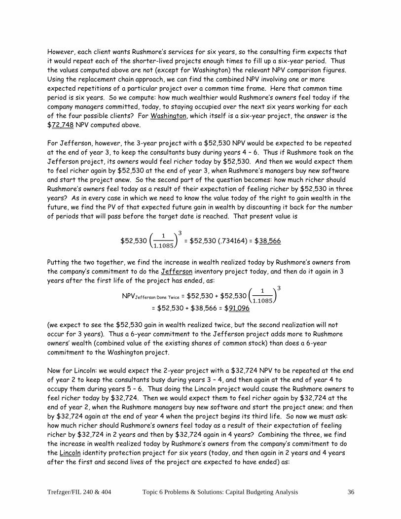
Trefzger/FIL 240 & 404 Topic 6 Problems & Solutions: Capital Budgeting Analysis 36
However, each client wants Rushmore’s services for six years, so the consulting firm expects that
it would repeat each of the shorter-lived projects enough times to fill up a six-year period. Thus
the values computed above are not (except for Washington) the relevant NPV comparison figures.
Using the replacement chain approach, we can find the combined NPV involving one or more
expected repetitions of a particular project over a common time frame. Here that common time
period is six years. So we compute: how much wealthier would Rushmore’s owners feel today if the
company managers committed, today, to staying occupied over the next six years working for each
of the four possible clients? For Washington, which itself is a six-year project, the answer is the
$72,748 NPV computed above.
For Jefferson, however, the 3-year project with a $52,530 NPV would be expected to be repeated
at the end of year 3, to keep the consultants busy during years 4 – 6. Thus if Rushmore took on the
Jefferson project, its owners would feel richer today by $52,530. And then we would expect them
to feel richer again by $52,530 at the end of year 3, when Rushmore’s managers buy new software
and start the project anew. So the second part of the question becomes: how much richer should
Rushmore’s owners feel today as a result of their expectation of feeling richer by $52,530 in three
years? As in every case in which we need to know the value today of the right to gain wealth in the
future, we find the PV of that expected future gain in wealth by discounting it back for the number
of periods that will pass before the target date is reached. That present value is
$52,530 (1
1.1085)
3 = $52,530 (.734164) = $38,566
Putting the two together, we find the increase in wealth realized today by Rushmore’s owners from
the company’s commitment to do the Jefferson inventory project today, and then do it again in 3
years after the first life of the project has ended, as:
NPVJefferson Done Twice = $52,530 + $52,530 (1
1.1085)
3
= $52,530 + $38,566 = $91,096
(we expect to see the $52,530 gain in wealth realized twice, but the second realization will not
occur for 3 years). Thus a 6-year commitment to the Jefferson project adds more to Rushmore
owners’ wealth (combined value of the existing shares of common stock) than does a 6-year
commitment to the Washington project.
Now for Lincoln: we would expect the 2-year project with a $32,724 NPV to be repeated at the end
of year 2 to keep the consultants busy during years 3 – 4, and then again at the end of year 4 to
occupy them during years 5 – 6. Thus doing the Lincoln project would cause the Rushmore owners to
feel richer today by $32,724. Then we would expect them to feel richer again by $32,724 at the
end of year 2, when the Rushmore managers buy new software and start the project anew; and then
by $32,724 again at the end of year 4 when the project begins its third life. So now we must ask:
how much richer should Rushmore’s owners feel today as a result of their expectation of feeling
richer by $32,724 in 2 years and then by $32,724 again in 4 years? Combining the three, we find
the increase in wealth realized today by Rushmore’s owners from the company’s commitment to do
the Lincoln identity protection project for six years (today, and then again in 2 years and 4 years
after the first and second lives of the project are expected to have ended) as:

Trefzger/FIL 240 & 404 Topic 6 Problems & Solutions: Capital Budgeting Analysis 37
NPVLincoln Done Three Times = $32,724 + $32,724 (1
1.1085)
2+ $32,724 (
1
1.1085)
4
= $32,724 + $26,631 + $21,673 = $81,028
So a 6-year commitment to the Lincoln project adds more to the owners’ wealth than does a 6-year
commitment to Washington, but less than would a 6-year commitment to Jefferson. Finally for
Roosevelt: we would expect the 1-year project with a $14,232 NPV to be repeated at the end of
each year to keep the consultants busy on an ongoing basis for six years. Thus committing to doing
the Roosevelt project would cause Rushmore’s owners to feel richer today by $14,232. Then we
would expect them to feel richer again by $14,232 at the end of each of years 1 – 5 (or think of it
as the start of years 2 – 6), when Rushmore starts the project again after each previous 1-year life
ends. So we ask: how much richer should Rushmore’s owners feel today through their expectation
of feeling richer by $14,232 today and also in 1, 2, 3, 4, and 5 years? Combining the six, the gain
in wealth they feel today from the commitment to do the Roosevelt virus project today (the end
of year 0), and then again at the ends of years 1 – 5 as each successive life of the project ends, is:
NPVRoosevelt Done Six Times = $14,232 + $14,232 (1
1.1085)
1
+ $14,232 (1
1.1085)
2
+ $14,232 (1
1.1085)
3 + $14,232 (
1
1.1085)
4+ $14,232 (
1
1.1085)
5
= $14,232 + $12,839 + $11,582 + $10,449 + $9,426 + $8,503 = $67,031
Now that we have considered each project over six years, with the expected repetitions factored
in, the four projects’ ranking is as follows: Jefferson ranked best at a $91,096 combined NPV;
Lincoln second with an $81,028 combined NPV; Washington third with a $72,478 combined NPV; and
Roosevelt last with a $67,031 combined NPV. Thus Rushmore will increase its owners’ wealth by the
highest possible amount by committing today to doing the 3-year Jefferson inventory project, with
the expectation that it will begin the whole process again at the end of year 3/start of year 4.
13. Aconcagua Fabricating is building a new production facility on its current factory site. During the two years it
will take to construct the new facility, Aconcagua will conduct many of its activities from temporary quarters 35
miles away. The company needs access to 5 passenger vans to move workers, as needed, between the two locations
during the three-year construction period. One option is to buy the vans, with expected net cash flows (all costs
paid in advance) of -$110,000 in year 0 (the purchase), -$12,500 in year 1 (for maintenance), and -$2,500 in year 2
(maintenance costs, net of the present value of a small resale price). The other possibility is to lease the vans, with
each year’s expected net cash flow totaling -$46,000 (an amount paid at the start of each year that includes all
maintenance). Based on net present value (NPV) analysis, with an 8.75% assumed annual weighted average cost of
capital, which choice should Aconcagua’s managers make? What is each option’s internal rate of return (IRR)?
Type: Computing NPVs for Projects with Negative Cash Flows Only. There are no expected revenues;
the firm’s customers make purchases based on product features and do not know or care where
the operations occur. Here we compare two projects based on the present values of their costs.
Buying the vans has different expected year-to-year cash flows, so we must use the general
NPV = CF0
(1 + r)0 +
CF1
(1 + r)1 +
CF2
(1 + r)2 +
CF3
(1 + r)3 + … +
CFn
(1 + r)n
form of the NPV equation: NPVBuying = −$110,000
(1.0875)0 +
−$12,500
(1.0875)1 +
−$2,500
(1.0875)2
= -$110,000 – $11,494 – $2,114 = –$123,608

Trefzger/FIL 240 & 404 Topic 6 Problems & Solutions: Capital Budgeting Analysis 38
With level expected cash flows at the start of each year for the leasing situation, we can more
efficiently compute the PV of the expected cash flow stream as the PV of a level annuity due:
NPVLeasing = -$46,000 [(1−(
1
1.0875)
3
.0875) (1.0875)] = -$46,000 (2.765094) = –$127,194
We always want to select the project with the highest expected net present value. In this case the
higher total means the NPV with the lower negative magnitude, which is associated with buying the
vans. (The need to operate temporarily over longer distances is a necessary cost that comes out of
the owners’ pockets, accepted in return for the wealth-enhancing features of the facility upgrade.)
[In fact the cost of having the vans might simply be viewed as component cash flows in the bigger
project of building the new facility.] What about the IRR? The average periodic rate of return
represented by a series of cash outflows, with no accompanying net inflows, is infinitely negative.
(In a similar manner, a series of cash inflows, with no accompanying net outflows, represents a
positively infinite average periodic rate of return; if you invest nothing and get even a penny back a
year later it is an infinitely high annual percentage return.) The cash flows must change directions
at least once for us to be able to compute a meaningful periodic percentage rate of return or cost.
14. Matterhorn Appliances is deciding whether to build a new, state-of-the-art production facility. The project
would involve making an initial investment today (at the end of year 0) and then require two more full years to
build, and thus would not be up and running (and generating sales revenues and resulting positive cash flows) until
year 3. Expected net cash flows would be as follows: -$17,750,000 in year 0; -$9,500,000 in year 1; -$8,000,000 in
year 2; and then $7,350,000 in each of years 3 through 17. If Matterhorn managers assume that the cost of capital
for this type investment is 13.25% per year, should they go ahead with the project? Compute the net present value
(NPV), profitability index (PI), internal rate of return (IRR), and modified internal rate of return (MIRR) in
determining your answer.
Type: Evaluating Project with Multiple Outlays. The unusual feature of this example is the series of
up-front negative cash flows before a series of positive cash flows is expected. We compute net
present value, based on the general net present value equation
NPV = CF0
(1 + r)0 +
CF1
(1 + r)1 +
CF2
(1 + r)2 +
CF3
(1 + r)3 + … +
CFn
(1 + r)n ,
as NPV = −$17,750,000
(1.1325)0 +
−$9,500,000
(1.1325)1 +
−$8,000,000
(1.1325)2 +
$7.300,000
(1.1325)3 + … +
$7,300,000
(1.1325)17
= −$17,750,000
(1.1325)0 +
−$9,500,000
(1.1325)1 +
−$8,000,000
(1.1325)2 + $7,350,000 (
1−(1
1.1325)
15
.1325) (
1
1.1325)
2
= -$17,750,000 – $8,388,521 – $6,237,543 + $7,350,000 (6.379793) (.779693)
= -$32,376,064 + $36,560,954 = $4,184,890
This project, if accepted, would be expected to increase the value of the owners’ common stock
by just over $4 million. We use the same two numbers in computing the profitability index, but
instead of subtracting the PV of the expected net inflows minus the PV of the expected net
outflows we divide the PV of the expected net inflows by the PV of the expected net outflows:
PI = $36,560,954
$32,376,064 = 1.129259 ;

Trefzger/FIL 240 & 404 Topic 6 Problems & Solutions: Capital Budgeting Analysis 39
the project is expected to generate $1.129259 – $1.00 = approximately $.13 in wealth for every
dollar invested. We would compute the internal rate of return with the equation:
= −$17,750,000
(1 + r)0 +
−$9,500,000
(1 + r)1 +
−$8,000,000
(1 + r)2 + $7,350,000 (
1−(1
1 + r)
15
r) (
1
1 + r)
2
With trial and error we would find the answer to be 15.2257%; let’s double-check:
= −$17,750,000
(1.152257)0 +
−$9,500,000
(1.152257)1 +
−$8,000,000
(1.152257)2 + $7,350,000 (
1−(1
1.152257)
15
.152257) (
1
1.152257)
2
= -$17,750,000 – $8,244,688 - $6,025,475 + $7,350,000 (5.784084) (.753184)
= -$32,020,163 + $32,020,163 = $0 ✓
With a positive NPV we knew that the IRR would have to be greater than the 13.25% annual cost of
capital. Note that this is a special case of a “normal” project, with the net cash outlays occurring
up-front, and with only one change in the direction of expected net cash flows, going from negative
in years 0 – 2 to positive in years 3 – 17. Note also that a financial calculator can greatly speed
up some of the computations, although it is difficult to see how anyone can understand what the
calculator is doing without first having learned the underlying relationships by setting up problems
manually. On the BA II Plus we would type CF 2nd CLR WRK, then 17750000 and the +/- key and
ENTER. Then hit the ↓ key to move to the next time period, and type 9500000 and the +/- key and
ENTER and hit the ↓ key twice. Then type 8000000 +/- ENTER ↓↓, 7350000 ENTER ↓ 15 ENTER ↓
NPV 13.25 ENTER ↓ CPT (screen should show the $4,184,890 NPV found earlier with our own
computations) and then IRR CPT (should show 15.225687 as the annual IRR percentage).
In computing the MIRR, we make an explicit assumption regarding managers’ reinvestment of
the positive expected net cash flows through the end of the project’s life. There are no special
computational steps needed here, because once the positive cash flows start we expect to simply
have a series of 15 end-of-period investments at a 13.25% annual rate of return:
PMT x FAC = TOT
$7,350,000 ((1.1325)15−1
.1325) = TOT
= $7,350,000 (41.245803) = $303,156,654 Terminal Value
Then we simply compute the indicated average annual rate of return, using the $32,376,064
present value of the year 0 – 2 expected outlays as the initial investment. But bear in mind that
even though there are only 15 years of expected $7,350,000 cash flows, 17 years are expected
to pass between the initial investment and the receipt of the last of those 15 positive amounts:
BAMT (1 + r)n = EAMT
$32,376,064 (1 + r)17 = $303,156,654
(1 + r)17 = 9.363604
√(1 + r)1717 = √9.36360417
(1 + r) = 9.3636041/17 = 9.363604.058824 = 1.140627
r = .140627 , or an annual MIRR of 14.0627%

Trefzger/FIL 240 & 404 Topic 6 Problems & Solutions: Capital Budgeting Analysis 40
We know that the annual MIRR (here, 14.0627%) should fall between the 13.25% annual cost of
capital and the 15.2257% annual IRR. In summary, building the new factory would seem to be
profitable in time value-adjusted terms. The positive NPV (with PI greater than 1) indicates that
the positive net cash flows would be high enough to pay back the initial 3-stage investment, plus
returns to the investors who supplied the money for the investment that cost 13.25% annually to
deliver, plus something extra to increase the value of the existing shares of common stock held by
the company’s owners). The annual IRR and MIRR exceeding the annual cost of capital indicates
that the project would earn an periodic rate of return that is more than would be needed to deliver
fair returns to the investors.
15. K2 Assurity sells multi-year insurance policies to owners of small commercial buildings. It typically charges
$18,000 in return for coverage over the subsequent four years. Experience with these kinds of policies indicates that
K2’s average financial-plus-administrative cost of paying claims on a building (when fires or other perils occur) will
be $5,150 per year. If the annual cost of capital is 7% (here we can think of it as the average annual rate of return
earned on the investment of premium dollars received), what NPV and IRR does K2 realize, on average, on these
policies (an insurance company must deal with large numbers of policies to have predictable outcomes)?
Type: Evaluating Non-Normal Project (Positive, then Negative, Cash Flows). This situation is somewhat
unusual, in that the company expects to realize a net cash inflow today and then incur its net cash
outflows at later dates. K2 may seem to be losing money on each contract; after all, the $5,150
x 4 = $20,600 it expects to spend paying claims exceeds the $18,000 received for providing the
insurance service. However, the NPV of a contract actually turns out to be slightly positive:
NPV = CF0
(1 + r)0 +
CF1
(1 + r)1 +
CF2
(1 + r)2 +
CF3
(1 + r)3 + … +
CFn
(1 + r)n
= $18,000
(1.07)0 +
−$5,150
(1.07)1 +
−$5,150
(1.07)2 +
−$5,150
(1.07)3 +
−$5,150
(1.07)4
= $18,000
(1.07)0 - $5,150 (
1−(1
1.07)
4
.07)
= $18,000 – $5,150 (3.387211) = $18,000 – $17,444 = $556
Thus K2’s owners realize a $556 increase in wealth every time a new policy is sold. As insurance
companies often do, K2 “loses” money on its direct insurance (so-called “underwriting”) activities,
while earning enough by reinvesting the premiums that it makes money overall. Because it does not
expect to pay claims until a later date, it can start with less today than it expects to pay out and
still end up covering all its costs, including a fair rate of return to K2’s money providers. (Note that
the $18,000 it receives today has a present value of $18,000, whereas the $5,150 it expects to pay
in year 4 has a present value of only -$3,929.) Trial and error would show the IRR to be 5.6240%
per year; let’s double-check:
NPV = $18,000
(1.056240)0 - $5,150 (
1−(1
1.056240)
4
.056240)
= $18,000 – $5,150 (3.495149) = $18,000 – $18,000 = $0 ✓
You are not expected to have a financial calculator for our class or to do trial & error computations;
just be able to set up or recognize the equation we would use in solving for IRR if there are multiple
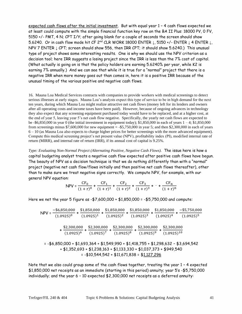
Trefzger/FIL 240 & 404 Topic 6 Problems & Solutions: Capital Budgeting Analysis 41
expected cash flows after the initial investment. But with equal year 1 – 4 cash flows expected we
at least could compute with the simple financial function key row on the BA II Plus: 18000 PV, 0 FV,
5150 +/- PMT, 4 N; CPT I/Y; after going blank for a couple of seconds the screen should show
5.6240. Or in cash flow mode hit CF 2nd CLR WORK 18000 ENTER ↓, 5150 +/- ENTER ↓ 4 ENTER ↓,
NPV 7 ENTER ↓ CPT; screen should show 556, then IRR CPT; it should show 5.6240.) This unusual
type of project shows some interesting results. One is why we should use the NPV criterion as a
decision tool; here IRR suggests a losing project since the IRR is less than the 7% cost of capital.
(What actually is going on is that the policy holders are earning 5.6240% per year, while K2 is
earning 7% annually.) And we can see that while it is true for a “normal” project that there is a
negative IRR when more money goes out than comes in, here it is a positive IRR because of the
unusual timing of the various positive and negative cash flows.
16. Mauna Loa Medical Services contracts with companies to provide workers with medical screenings to detect
serious illnesses at early stages. Mauna Loa’s analysts expect this type of service to be in high demand for the next
ten years, during which Mauna Loa might realize attractive net cash flows (money left for its lenders and owners
after all operating costs and income taxes have been paid). However, because of ongoing advances in technology
they also expect that any screening equipment purchased today would have to be replaced, and at a higher cost, at
the end of year 5, leaving year 5’s net cash flow negative. Specifically, the yearly net cash flows are expected to
be -$6,850,000 in year 0 (the initial investment in equipment today); $1,850,000 in each of years 1 – 4; $1,850,000
from screenings minus $7,600,000 for new equipment = -$5,750,000 in year 5; and then $2,300,000 in each of years
6 – 10 (as Mauna Loa also expects to charge higher prices for better screenings with the more advanced equipment).
Compute this medical screening project’s net present value (NPV), profitability index (PI), modified internal rate of
return (MIRR), and internal rate of return (IRR), if its annual cost of capital is 9.25%.
Type: Evaluating Non-Normal Project (Alternating Positive, Negative Cash Flows). The issue here is how a
capital budgeting analyst treats a negative cash flow expected after positive cash flows have begun.
The beauty of NPV as a decision technique is that we do nothing differently than with a “normal”
project (negative net cash flow/flows initially and then positive net cash flows thereafter), other
than to make sure we treat negative signs correctly. We compute NPV, for example, with our
general NPV equation:
NPV = CF0
(1 + r)0 +
CF1
(1 + r)1 +
CF2
(1 + r)2 +
CF3
(1 + r)3 + … +
CFn
(1 + r)n
Here we net the year 5 figure as -$7,600,000 + $1,850,000 = -$5,750,000 and compute:
NPV = −$6,850,000
(1.0925)0 +
$1,850,000
(1.0925)1 +
$1,850,000
(1.0925)2 +
$1,850,000
(1.0925)3 +
$1,850,000
(1.0925)4 +
−$5,750,000
(1.0925)5
+ $2,300,000
(1.0925)6 +
$2,300,000
(1.0925)7 +
$2,300,000
(1.0925)8 +
$2,300,000
(1.0925)9 +
$2,300,000
(1.0925)10
= -$6,850,000 + $1,693,364 + $1,549,990 + $1,418,755 + $1,298,632 – $3,694,542
+ $1,352,693 + $1,238,163 + $1,133,330 + $1,037,373 + $949,540
= -$10,544,542 + $11,671,838 = $1,127,296
Note that we also could group some of the cash flows together, treating the year 1 – 4 expected
$1,850,000 net receipts as an immediate (starting in this period) annuity; year 5’s -$5,750,000
individually; and the year 6 – 10 expected $2,300,000 net receipts as a deferred annuity:

Trefzger/FIL 240 & 404 Topic 6 Problems & Solutions: Capital Budgeting Analysis 42
NPV = −$6,850,000
(1.0925)0 + $1,850,000 (
1−(1
1.0925)
4
.0925) +
−$5,750,000
(1.0925)5
+ $2,300,000 (1−(
1
1.0925)
5
.0925) (
1
1.0925)
5 = -$10,544,542 + $11,671,838 = $1,127,296
(Mauna Loa expects to net $2,300,000 in each of years 6 – 10, which is a 5-year period starting
after 5 years have passed). We can get the same NPV answer by breaking the year 5 expected
cash flows into the outflow for the new equipment and the inflow from the ongoing sale of screening
services:
NPV = [−$6,850,000
(1.0925)0 +
−$7,600,000
(1.0925)5] + $1,850,000 (
1−(1
1.0925)
5
.0925)
+ $2,300,000 (1−(
1
1.0925)
5
.0925) (
1
1.0925)
5 = -$11,733,221 + $12,860,517 = $1,127,296
With NPV analysis it does not matter whether we treat the positive and negative expected year 5
cash flows as two separate figures or a net amount. So the changing directions on expected net
cash flows do not cause difficulty in computing NPV, as long as we keep the negative signs straight.
And with a positive NPV we know that the project appears profitable in a time value-adjusted
sense: it would be expected to return lenders’ and owners’ invested money, plus returns on that
investment that cost the managers 9.25% per year to deliver, and also increase the value of Mauna
Loa owners’ existing shares of common stock by a combined $1,127,296.
But the other techniques might leave us with less certain outcomes. For profitability index we get
slightly different answers depending on whether we treat the year 5 result as one net figure or two
separate amounts (although either way PI comes out to be approximately 1.10, which is greater than
1 as should occur since NPV is positive):
PI = $11,671,838
$10,544,542 = 1.106908 (or PI =
$12,860,517
$11,733,221 = 1.096077)
With modified internal rate of return, we also get different answers depending on the year 5
treatment. If we net out the positive and negative year 5 cash flow figures the initial investment
is seen as $10,544,542, and the terminal value of the reinvested positive cash flows is found with
year-by-year compounding (with year 5’s cash flow already having been accounted for) as:
Year Expected Year-End Cash Flow Reinvestment Factor Terminal Value
1 $1,850,000 (1.0925)9 $ 4,101,708
2 $1,850,000 (1.0925)8 $ 3,754,424
3 $1,850,000 (1.0925)7 $ 3,436,544
4 $1,850,000 (1.0925)6 $ 3,145,578
6 $2,300,000 (1.0925)4 $ 3,276,526
7 $2,300,000 (1.0925)3 $ 2,999,108
8 $2,300,000 (1.0925)2 $ 2,745,179
9 $2,300,000 (1.0925)1 $ 2,512,750
10 $2,300,000 (1.0925)0 $ 2,300,000
Total $28,271,817

Trefzger/FIL 240 & 404 Topic 6 Problems & Solutions: Capital Budgeting Analysis 43
or, as the future value of an annuity added to the FV of a “truncated annuity” as we called it in our
basic time value coverage:
$1,850,000 [((1.0925)
4−1
.0925) (1.0925)
6] + $2,300,000 (
(1.0925)5−1
.0925)
= $1,850,000 (7.804461) + $2,300,000 (6.014593)
= $14,438,253 + $13,833,564 = $28,271,817 Terminal Value
Then we simply compute the indicated average annual rate of return, as we always do:
BAMT (1 + r)n = EAMT
$10,544,542 (1 + r)10 = $28,271,817
(1 + r)10 = 2.681180
√(1 + r)1010 = √2.68118010
(1 + r) = 2.6811801/10 = 2.681180.10 = 1.103653
So r = annual MIRR = 10.3653%
(NPV is positive, so we would expect MIRR to be above the 9.25% annual cost of capital. However,
if we separate the two year 5 cash flow components then the initial investment is treated as the
slightly higher $11,733,721 combined PV of the two negative expected cash flows, and the terminal
value is the $28,271,817 computed above plus $1,850,000 (1.0925)5 = $2,879,247 = $31,151,064,
for a slightly lower computed MIRR:
$11,733,221 (1 + r)10 = $31,151,064
(1 + r)10 = 2.654946 so √(1 + r)1010 = √2.65494610
(1 + r) = 2.6549461/10 = 2.654946.10 = 1.102568
So r = annual MIRR = 10.2568%
We would tend to view the initial approach, with a year 5 cash flow that nets positive and negative
components to a -$5,750,000 total, as computationally correct for finding PIs and MIRRs. (Note
that the BA II Plus financial calculator and Microsoft Excel’s automated NPV/IRR/MIRR functions
allow only one net cash flow figure to be entered for any time period. 10.3653% is the MIRR figure
generated by Excel for this problem; the BA II Plus does not have an automated MIRR capability.)
But the truly unusual result is seen in computing internal rate of return. Recall the potential for
there to be one solution to the IRR equation for every directional change in the expected net cash
flows. Here the flows go from negative in year 0 to positive in years 1 – 4, then to negative again in
year 5 and back to positive in years 6 – 10. With three directional changes there potentially could
be three solutions, although here there happen to be only two, 12.7242% and -202.5884%. (You
could find them by creating an NPV profile and seeing what discount rates caused NPV to be $0.)
Double-check:
NPV = −$6,850,000
(1.127242)0 + $1,850,000 (
1−(1
1.127242)
4
.127242) +
−$5,750,000
(1.127242)5
+ $2,300,000 (1−(
1
1.127242)
5
.127242) (
1
1.127242)
5 = $ 0 ✓ and

Trefzger/FIL 240 & 404 Topic 6 Problems & Solutions: Capital Budgeting Analysis 44
NPV = −$6,850,000
(−1.025884)0 + $1,850,000 (
1−(1
−1.025884)
4
−2.025884) +
−$5,750,000
(−1.025884)5
+ $2,300,000 (1−(
1
−1.025884)
5
−2.025884) (
1
−1.025884)
5 = $ 0 ✓
The latter equation might look strange, but note that -202.5884% is -2.025884, such that (1 + r)
in this case is 1 – 2.025884 = -1.025884. Which of the two rates is the “correct” one? Both are
correct in a technical sense, though with a positive NPV we might feel more confident believing the
12.7242% (which would make sense as a number combined with a 9.25% reinvestment rate to give
an MIRR of 10.3653% per year). The reason why -202% also solves the equation is that with a big
negative discount rate the year 5 net expenditure actually has a positive present value, which helps
offset the negative value of the year 0 cash flow.
17. Return to the story of Ms. McKinley in earlier problem 2. The Denali Art Gallery owner just paid $250,000
for a painting that she expects to hold for 20 years and then sell for $8,000,000, and she attributes a 15% annual
weighted average cost of capital to this type of investment. We computed the net present value, profitability index,
internal rate of return, and modified internal rate of return based on an assumption that no other cash flows would
be relevant to the analysis – for example, she had not considered a differential annual security cost for holding
this painting because her gallery already is insured. But now Ms. McKinley learns that unusual features of this
particular art work would lead to an extra annual cost for insurance, maintenance, and secure storage, expected to be
$25,000 paid at the start of each of years 1 through 20. Taking this new information into account, what would we
compute her NPV, PI, IRR, and MIRR for this investment to be? What would these values be if the security costs
related to holding the painting were expected to be $35,000 per year?
Type: Evaluating Project with Multiple Expected Negative and One Expected Positive Cash Flows. One of the
many attractive features of NPV as a tool for analysis is that unusual patterns in the directions of
the cash flows cause no problems; we need merely keep the negative signs straight. Here we have
an initial investment of $250,000 at the end of year 0 and a separate payment, at the same time,
of $25,000 as the first year’s security cost (for a total period 0 cash flow of -$275,000). Then
at the end of each of years 1 through 19 (equivalent to the start of years 2 through 20) there is
another $25,000 expected outlay, and then a sole inflow of $8,000,000 is projected for the end
of year 20. Net present value, computed with the general NPV equation, is
NPV = -$275,000 (1
1.15)
0
+ -$25,000 (1
1.15)
1
+ … + -$25,000 (1
1.15)
19
+ $8,000,000 (1
1.15)
20
NPV = −$275,000
(1.15)0 +
−$25,000
(1.15)1 +
−$25,000
(1.15)2 + … +
−$25,000
(1.15)18 +
−$25,000
(1.15)19 +
$8,000,000
(1.15)20
= −$275,000
(1.15)0 + (-$25,000) (
1−(1
1.15)
19
.15) +
$8,000,000
(1.15)20
= -$275,000 + (-$25,000) (6.198231) + $8,000,000 (.061100)
= -$275,000 - $154,955.78 + $488,802.23 = -$429,955.78 + $488,802.23 = $58,846.45
NPV is a measure of how much the investment adds to the project owner’s wealth. After taking
into account the previously ignored holding costs Ms. McKinley feels wealthier, as a result of buying
the painting, by a little less than $59,000 (vs. a roughly $239,000 measured wealth gain before the

Trefzger/FIL 240 & 404 Topic 6 Problems & Solutions: Capital Budgeting Analysis 45
holding costs were considered). The project is not as good as originally had been thought, because
now we recognize greater ongoing costs with no accompanying increase in benefits. Profitability
Index is a proportional measure based on the same two summary values as NPV: PV of expected
cash inflows divided by PV of expected cash outflows (vs. NPV’s PV of expected cash inflows minus
PV of expected cash outflows).
NPV = $488,802.23 - $404,955.78 = $58,846.45
PI = $488,802.23 ÷ $404,955.78 = 1.207051
Purchasing the painting gives Ms. McKinley an increase in wealth of just $.207 for every dollar
invested – not too bad, but not as good as the $.955 in NPV for every dollar invested that had been
computed when yearly holding costs were not included in the computations. Incidentally, with no
cash expected to be received until the end of year 20 when the project ends, the payback and
discounted payback periods both remain at 20 years, as they were found to be in problem 2.
Internal rate of return is computed with the same equation used in solving for NPV, but with NPV
set strategically equal to $0 and the discount rate as the unknown to solve for:
$0 = −$275,000
(1+𝑟)0 + (-$25,000) (
1−(1
1+r)
19
r) +
$8,000,000
(1+𝑟)20
The rate that solves is 15.83109819% (thanks to Excel for handling the messy trial and error steps
painlessly for us); note when that percentage rate is plugged in as the discount rate we get
−$275,000
(1.1583109819)0 + (-$25,000) (
1−(1
1.1583109819)
19
.1583109819) +
$8,000,000
(1.1583109819)20
= -$275,000 + (-$25,000) (5.929592) + $8,000,000 (.052905)
= -$275,000 + (-$148,239.81) + $423,239.82
= -$423,239.81 + $423,239.81 = $0 ✓
Because Ms. McKinley expects to get back $8,000,000 after investing only $250,000 + (20)
($25,000) or $275,000 + (19) ($25,000) = $750,000, her expected average annual rate of return
(the IRR) obviously is positive. And because NPV is positive, we knew that the average annual rate
of return represented by this cash flow series had to exceed the 15% annual weighted average cost
of capital. But now it is only a small percentage higher than the cost of capital, not the much higher
18.9207% represented by simply spending $250,000 and getting $8,000,000 back 20 years later.
And now that there are intermediate-period cash flows to consider, MIRR is not equal to IRR as it
was in problem 2. MIRR reflects a direct analysis of reinvestment experience between the date
when a cash flow is expected and the end of the project’s life. But in this situation the impact is
the opposite of reinvesting; we consider the present value benefit of not having to pay the various
$25,000 outlays in years 1 to 19 until some investment earnings have accumulated. So we compute
the indicated average annual rate of return, using $8,000,000 as the terminal value and the
$429,955.78 present value of the year 0 – 19 expected outlays as the initial investment (recall that
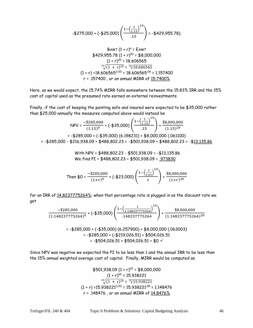
Trefzger/FIL 240 & 404 Topic 6 Problems & Solutions: Capital Budgeting Analysis 46
-$275,000 + (-$25,000) (1−(
1
1.15)
19
.15) = -$429,955.78).
BAMT (1 + r)n = EAMT
$429,955.78 (1 + r)20 = $8,000,000
(1 + r)20 = 18.606565
√(1 + r)2020 = √18.60656520
(1 + r) =18.6065651/20 = 18.606565.05 = 1.157400
r = .157400 , or an annual MIRR of 15.7400%
Here, as we would expect, the 15.74% MIRR falls somewhere between the 15.83% IRR and the 15%
cost of capital used as the presumed rate earned on external reinvestments.
Finally, if the cost of keeping the painting safe and insured were expected to be $35,000 rather
than $25,000 annually the measures computed above would instead be
NPV = −$285,000
(1.15)0 + (-$35,000) (
1−(1
1.15)
19
.15) +
$8,000,000
(1.15)20
= -$285,000 + (-$35,000) (6.198231) + $8,000,000 (.061100)
= -$285,000 - $216,938.09 + $488,802.23 = -$501,938.09 + $488,802.23 = -$13,135.86
With NPV = $488,802.23 - $501,938.09 = -$13,135.86
We find PI = $488,802.23 ÷ $501,938.09 = .973830
Then $0 = −$285,000
(1+𝑟)0 + (-$23,000) (
1−(1
1+r)
19
r) +
$8,000,000
(1+𝑟)20
for an IRR of 14.8237775264%; when that percentage rate is plugged in as the discount rate we
get
−$285,000
(1.148237775264)0 + (-$35,000) (
1−(1
1.148237775264)
19
.148237775264) +
$8,000,000
(1.148237775264)20
= -$285,000 + (-$35,000) (6.257900) + $8,000,000 (.063003)
= -$285,000 + (-$219,026.51) + $504,026.51
= -$504,026.51 + $504,026.51 = $0 ✓
Since NPV was negative we expected the PI to be less than 1 and the annual IRR to be less than
the 15% annual weighted average cost of capital. Finally, MIRR would be computed as
$501,938.09 (1 + r)20 = $8,000,000
(1 + r)20 = 15.938221
√(1 + r)2020 = √15.93822120
(1 + r) =15.9382211/20 = 15.938221.05 = 1.148476
r = .148476 , or an annual MIRR of 14.8476%
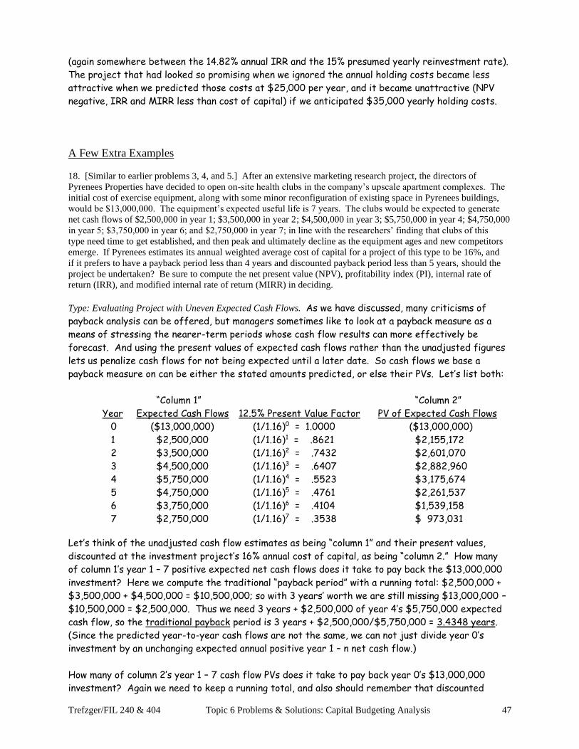
Trefzger/FIL 240 & 404 Topic 6 Problems & Solutions: Capital Budgeting Analysis 47
(again somewhere between the 14.82% annual IRR and the 15% presumed yearly reinvestment rate).
The project that had looked so promising when we ignored the annual holding costs became less
attractive when we predicted those costs at $25,000 per year, and it became unattractive (NPV
negative, IRR and MIRR less than cost of capital) if we anticipated $35,000 yearly holding costs.
A Few Extra Examples
18. [Similar to earlier problems 3, 4, and 5.] After an extensive marketing research project, the directors of
Pyrenees Properties have decided to open on-site health clubs in the company’s upscale apartment complexes. The
initial cost of exercise equipment, along with some minor reconfiguration of existing space in Pyrenees buildings,
would be $13,000,000. The equipment’s expected useful life is 7 years. The clubs would be expected to generate
net cash flows of $2,500,000 in year 1; $3,500,000 in year 2; $4,500,000 in year 3; $5,750,000 in year 4; $4,750,000
in year 5; $3,750,000 in year 6; and $2,750,000 in year 7; in line with the researchers’ finding that clubs of this
type need time to get established, and then peak and ultimately decline as the equipment ages and new competitors
emerge. If Pyrenees estimates its annual weighted average cost of capital for a project of this type to be 16%, and
if it prefers to have a payback period less than 4 years and discounted payback period less than 5 years, should the
project be undertaken? Be sure to compute the net present value (NPV), profitability index (PI), internal rate of
return (IRR), and modified internal rate of return (MIRR) in deciding.
Type: Evaluating Project with Uneven Expected Cash Flows. As we have discussed, many criticisms of
payback analysis can be offered, but managers sometimes like to look at a payback measure as a
means of stressing the nearer-term periods whose cash flow results can more effectively be
forecast. And using the present values of expected cash flows rather than the unadjusted figures
lets us penalize cash flows for not being expected until a later date. So cash flows we base a
payback measure on can be either the stated amounts predicted, or else their PVs. Let’s list both:
“Column 1” “Column 2”
Year Expected Cash Flows 12.5% Present Value Factor PV of Expected Cash Flows
0 ($13,000,000) (1/1.16)0 = 1.0000 ($13,000,000)
1 $2,500,000 (1/1.16)1 = .8621 $2,155,172
2 $3,500,000 (1/1.16)2 = .7432 $2,601,070
3 $4,500,000 (1/1.16)3 = .6407 $2,882,960
4 $5,750,000 (1/1.16)4 = .5523 $3,175,674
5 $4,750,000 (1/1.16)5 = .4761 $2,261,537
6 $3,750,000 (1/1.16)6 = .4104 $1,539,158
7 $2,750,000 (1/1.16)7 = .3538 $ 973,031
Let’s think of the unadjusted cash flow estimates as being “column 1” and their present values,
discounted at the investment project’s 16% annual cost of capital, as being “column 2.” How many
of column 1’s year 1 – 7 positive expected net cash flows does it take to pay back the $13,000,000
investment? Here we compute the traditional “payback period” with a running total: $2,500,000 +
$3,500,000 + $4,500,000 = $10,500,000; so with 3 years’ worth we are still missing $13,000,000 –
$10,500,000 = $2,500,000. Thus we need 3 years + $2,500,000 of year 4’s $5,750,000 expected
cash flow, so the traditional payback period is 3 years + $2,500,000/$5,750,000 = 3.4348 years.
(Since the predicted year-to-year cash flows are not the same, we can not just divide year 0’s
investment by an unchanging expected annual positive year 1 – n net cash flow.)
How many of column 2’s year 1 – 7 cash flow PVs does it take to pay back year 0’s $13,000,000
investment? Again we need to keep a running total, and also should remember that discounted

Trefzger/FIL 240 & 404 Topic 6 Problems & Solutions: Capital Budgeting Analysis 48
payback always is longer than traditional payback (it takes more of the smaller, discounted dollar
measures to repay the original investment, meaning that it takes longer to give the lenders and
owners back their original investment plus fair returns on that investment than it takes to repay
the investment alone). So we might expect to total 4 or 5 of the discounted cash flows before
getting close to the $13,000,000 target. $2,155,172 + $2,601,070 + $2,882,960 + $3,175,674 =
$10,814,876, short of the target by $13,000,000 – $10,814,876 = $2,185,124. That amount is
slightly less than year 5’s $2,261,537, so discounted payback period is 4 + $2,185,124/$2,261,537 =
4.9662 years. Thus the project is acceptable under the company’s expressed (and, critics would
say, arbitrary; there is no theoretical basis for the 4 and 5 year limits) payback guidelines.
Our more systematic methods for evaluating a proposed capital investment project are net present
value (NPV), profitability index (PI), internal rate of return (IRR), and modified internal rate of
return (MIRR). Recall that our general net present value equation is
NPV = CF0
(1 + r)0 +
CF1
(1 + r)1 +
CF2
(1 + r)2 +
CF3
(1 + r)3 + … +
CFn
(1 + r)n
Here the post-period 0 net cash flows are not expected to be the same from year to year over the
project’s life, so we must treat each one separately in our computations. Thus the NPV is computed
(leaving off the 000s for computational ease) as:
NPV = −$13,000
(1.16)0 +
$2,500
(1.16)1 +
$3,500
(1.16)2 +
$4,500
(1.16)3 +
$5,750
(1.16)4 +
$4,750
(1.16)5 +
$3,750
(1.16)6 +
$2,750
(1.16)7
= -$13,000 + $2,155.172 + $2,601.070 + $2,882.960 + $3,175.674 + $2,261.537
+ $1,539.158 + $973.031 = -$13,000 + $15,588.602 = $2,588.602 ,
which now we can translate back to full dollar figures as $2,588,602. With a positive measured
NPV the project should be accepted. If Pyrenees decides to open the health clubs in its apartment
buildings, it expects to have positive year 1 – 7 net cash flows, which means it should be able to
pay the clubs’ operating expenses, along with income taxes, and have money left for the company’s
lenders and owners. But simply expecting to have money left for the money providers (positive
net cash flows) does not mean the investment project is a good one. The net cash flows must be
positive enough in years 1 – n to repay the lenders and owners for making the year 0 investment,
plus a fair (here, costing 16% per year for the managers to deliver) annual rate of return on that
money. That amount would result in a $0 NPV, which is just enough that management could expect
to provide everyone involved in the operation (from workers to vendors to providers of government
services to providers of money) with fair financial returns. A positive NPV goes a step farther,
providing not just a minimally acceptable return to all, but an increase in the owners’ wealth (any
extra belongs to the owners). The $2,588,602 NPV means that Pyrenees expects to provide a fair
basic return to the lenders and owners at a 16% average yearly cost, and also to increase the total
value of the existing shares of Pyrenees common stock by $2,588,602. If there were 1 million
shares outstanding, we would expect the value of each to rise by about $2.59 once the market
learns that the company has committed to this new, wealth-enhancing project.
Whereas NPV is the present value of the expected net cash inflows minus the present value of the
expected net cash outflows (in a simple project, the initial investment), profitability index (PI) is
the present value of the expected net cash inflows divided by the present value of the net cash
outflows. So here we have not $15,588,602 – $13,000,000, but rather $15,588,602 ÷ $13,000,000:

Trefzger/FIL 240 & 404 Topic 6 Problems & Solutions: Capital Budgeting Analysis 49
PI = $15,588,602
$13,000,000 = 1.1991
Every dollar invested is expected to generate $1.1991 – $1.00 = almost $.20 in NPV. PI is a relative
NPV measure, telling how much NPV is generated per dollar invested. (If NPV is positive then PI is
greater than 1.0.) We might expect a large project to have a large NPV and a small project a small
NPV, but how well does each do proportionally in creating wealth for the owners? (Some analysts
view PI as a pointless measure, since owners should care about wealth, not proportional wealth.)
We compute IRR with that same NPV equation, setting NPV strategically equal to $0 and using trial
and error to solve for r (instead of using a known r, the periodic cost of capital, and solving directly
for NPV). So to solve for IRR we find the discount rate that makes the NPV = $0 equation hold
true (in other words, we find the discount rate that sets PV of cash inflows = PV of cash outflows).
[With NPV we know the discount rate and solve for the dollar value; with IRR we know the dollar
value ($0) and solve for the discount rate.] Here we have:
$0 = −$13,000
(1 + r)0 +
$2,500
(1 + r)1 +
$3,500
(1 + r)2 +
$4,500
(1 + r)3 +
$5,750
(1 + r)4 +
$4,750
(1 + r)5 +
$3,750
(1 + r)6 +
$2,750
(1 + r)7
With trial and error we would find that 22.144% is the IRR that solves the equation:
NPV = −$13,000
(1.22144)0 + $2,500
(1.22144)1 + $3,500
(1.22144)2 + $4,500
(1.22144)3 + $5,750
(1.22144)4 + $4,750
(1.22144)5 + $3,750
(1.22144)6 + $2,750
(1.22144)7
= -$13,000 + $2,046.764 + $2,345.977 + $2,469.426 + $2,583.326 + $1,747.161
+ $1,129.272 + $677.997 = -$13,000 + $13,000 = $0 ✓
Only by earning a rate of return greater than the cost of the money could the company managers
deliver fair returns to the money providers and have something left over to increase the value of
the firm’s common equity. So with a positive NPV we knew that the annual IRR had to exceed the
16% annual cost of capital. In our trial and error computations, when we pretend that money costs
22.144% we get a $0 NPV, suggesting that the rate of return present in these expected cash flows
is 22.144%: only with a 22.144% annual return on the investment could the managers deliver returns
to the investors that cost 22.144% each year to deliver, and have no money over and no shortage.
(With the BA II Plus we would type CF 2nd CLR WORK, 13000 +/- ENTER ↓, 2500 ENTER ↓↓, 3500
ENTER ↓↓, 4500 ENTER ↓↓, 5750 ENTER ↓↓, 4750 ENTER ↓↓, 3750 ENTER ↓↓, 2750 ENTER ↓, IRR
CPT, screen should go blank briefly and then show 22.143793; then could also type NPV 16 ENTER ↓
CPT, screen should quickly show 2,588.602398 in keeping with the NPV we computed above.)
Some analysts criticize the IRR measure because it does not account directly for reinvesting the
expected positive net cash flows through the end of year n. With modified internal rate of return
(MIRR) we do look directly at how expected reinvesting affects the measured overall percentage
rate of return (we treat the project’s life as a unified whole). Treating the 16% annual cost of
capital as the reinvestment rate (on the logic that the company already would have invested in any
project with a periodic rate of return greater than its periodic cost of money), we compute:

Trefzger/FIL 240 & 404 Topic 6 Problems & Solutions: Capital Budgeting Analysis 50
Year Expected Year-End Cash Flow Reinvestment Factor Terminal Value
1 $2,500,000 (1.16)6 $6,090,991
2 $3,500,000 (1.16)5 $7,351,196
3 $4,500,000 (1.16)4 $8,147,877
4 $5,750,000 (1.16)3 $8,975,152
5 $4,750,000 (1.16)2 $6,391,600
6 $3,750,000 (1.16)1 $4,350,000
7 $2,750,000 (1.16)0 $2,750,000
Total $44,056,816
Reinvesting each of the year 1 – 7 net cash flows at a 16% annual rate, we would expect to have a
year 7 ending balance of $44,056,816. (Because in our computations we treat the cash flows as
being available at the end of each year, year 7’s expected $2,750,000 can not be reinvested for
even one period.) So a $13,000,000 initial cash investment is expected to result, 6 years later, in
Pyrenees having $44,056,816 for its lenders and owners. The overall average annual rate of return
represented by these dollar figures can be computed as a simple annual rate of return:
BAMT (1 + r)n = EAMT
$13,000,000 (1 + r)7 = $44,056,816
(1 + r)7 = 3.388986
√(1 + r)77 = √3.3889867
(1 + r) = 3.3889861/7 = 3.388986.142857 = 1.190486
r = .190486 , or an annual MIRR of 19.0486%
MIRR blends the IRR with the assumed reinvestment rate, so its magnitude should be somewhere
between those two values (19.0486% is between the 16% annual cost of capital and the 22.144%
annual IRR).
Based on all 6 of the decision rules we considered, the Pyrenees managers should commit to doing
the project. NPV is positive (and therefore the PI is greater than 1), and the annual IRR and MIRR
both exceed the annual cost of capital. Thus the project is expected to create wealth for the
company’s owners, by delivering a periodic rate of return that exceeds the periodic weighted
average cost of providing acceptable financial returns to the lenders and owners (with anything
extra belonging to the owners), and that also is expected to provide for recouping the $13,000,000
in an acceptably short time based on payback measures.
19. [Combines aspects of earlier problems 3, 4, and 6.] The managers of Olympus Greenhouses foresee increased
demand for hydroponically-grown tomatoes and other vegetables, and therefore wants to develop a hydroponics
operation. The total cost of building specialized new facilities and obtaining all needed equipment and related items
is expected to be $18,500,000. The buildings and equipment are expected to be productive for 12 years. Net cash
flows (money remaining for the company’s lenders and owners, after all other parties including the applicable
government taxing bodies have been paid) is expected to be $3,395,000 in each year of the project’s expected 12-
year life. If Olympus managers prefer projects with a payback period of less than 5 years and a discounted payback
less than 7.5 years, and if they feel that the annual weighted average cost of capital for an expansion project of this
type is 11.25%, should the new equipment be purchased? What if instead the annual cost of capital were 18.25%?
Type: Evaluating Expansion Project with Equal Expected Cash Flows. To compute either traditional payback
or discounted payback, we determine how many of the year 1 – n expected net cash flow measures
will be needed to repay the initial year 0 investment in long-lived assets. But recall we can choose
as our year 1 – n measure either the unadjusted cash flows or their present values. Here:

Trefzger/FIL 240 & 404 Topic 6 Problems & Solutions: Capital Budgeting Analysis 51
“Column 1” “Column 2”
Year Expected Cash Flows 12.5% Present Value Factor PV of Expected Cash Flows
0 ($18,500,000) (1/1.1125)0 = 1.0000 ($18,500,000)
1 $3,395,000 (1/1.1125)1 = .8989 $3,051,685
2 $3,395,000 (1/1.1125)2 = .8080 $2,743,088
3 $3,395,000 (1/1.1125)3 = .7263 $2,465,697
4 $3,395,000 (1/1.1125)4 = .6528 $2,216,357
5 $3,395,000 (1/1.1125)5 = .5868 $1,992,231
6 $3,395,000 (1/1.1125)6 = .5275 $1,790,769
7 $3,395,000 (1/1.1125)7 = .4741 $1,609,680
8 $3,395,000 (1/1.1125)8 = .4262 $1,446,904
9 $3,395,000 (1/1.1125)9 = .3831 $1,300,588
10 $3,395,000 (1/1.1125)10 = .3443 $1,169,067
11 $3,395,000 (1/1.1125)11 = .3095 $1,050,847
12 $3,395,000 (1/1.1125)12 = .2782 $ 944,582
Again we can think of the unadjusted cash flow estimates as being in “column 1” and their present
values in “column 2.” In computing the traditional payback period we ask: how many of column 1’s
$3,395,000 expected net cash flows does it take to repay an $18,500,000 investment? Running
total: $3,395,000 + $3,395,000 + $3,395,000 + $3,395,000 + $3,395,000 = $16,975,000, short of
the target by $18,500,000 – $16,975,000 = $1,525,000. It takes 5 full years plus $1,525,000 of
the $3,395,000 year 6 figure, or 5 + $1,525/$3,395 = 5.4492 years. Or with all the post-year 0
cash flows expected to be equal, we can simply divide $18,500,000 ÷ $3,395,000 = 5.4492 years.
In computing the discounted payback period we ask: how many of column 2’s PVs of expected net
cash flows does it take to pay back the $18,500,000 investment? We know that the answer will
exceed the 5.4492-year traditional payback measure; it takes more of the small “Column 2” values
to repay $18,500,000 than it takes of the larger “Column 1” values. (Stated slightly differently:
it takes longer to provide the lenders and owners with a return of their investment plus acceptable
annual returns on that investment than it takes to repay the investment alone.) Running total: the
first 8 PVs sum to $3,051,685 + $2,743,088 + $2,465,697 + $2,216,357 + $1,992,231 + $1,790,769
+ $1,609,680 + $1,446,904 = $17,316,411. That value is $18,500,000 – $17,316,411 = $1,183,589
short of the target. So it takes 8 full years plus $1,183,589 of the year 9 $1,300,588 present
value, or 9 + $1,183,589/$1,300,588 = 8.9100 years as the discounted payback period. Or with
all expected post year 0 cash flows equal, we can set the problem up as a present value of a level
ordinary annuity and solve for n:
PMT x FAC = TOT
$3,395,000 (1−(
1
1.1125)
n
.1125) = $18,500,000
(1−(
1
1.1125)
n
.1125) = 5.44919
1 − (1
1.1125)
n= .613034 so 1 – (.898876)n = .613034
(.898876)n = .386966
n (ln .898876) = ln .386966
n (– .106610) = – .949418
n = 8.9055 years

Trefzger/FIL 240 & 404 Topic 6 Problems & Solutions: Capital Budgeting Analysis 52
(a slight difference from the answer above, because the latter approach keeps the curvilinear
relationship intact while the running total treats the cash flows linearly after we take their present
values). So if the post-year 0 cash flows all are projected to be the same, dividing the initial
investment by the unchanging annual cash flow yields the ordinary payback period, which is equal to
the PV of a level ordinary annuity factor with an unknown n that is the discounted payback period.
We see that on both the traditional payback and discounted payback measures the project violates
the standard that management prefers to meet. However, as this standard is only a preference
in this instance the project still might be considered if it appears sound under other criteria.
What do those other criteria suggest? With equal expected net cash flows after the initial
investment has been made, we can achieve the general net present value equation’s result of
NPV = CF0
(1 + r)0 +
CF1
(1 + r)1 +
CF2
(1 + r)2 +
CF3
(1 + r)3 + … +
CFn
(1 + r)n
simply by computing
NPV = −$18,500,000
(1.1125)0 + $3,395,000 (
1−(1
1.1125)
12
.1125)
= -$18,500,000 + $3,395,000 (6.415757)
= -$18,500,000 + $21,781,496 = $3,281,496
With NPV computed here as $21,781,496 minus $18,500,000 (PV of expected net cash inflows
minus PV of expected net cash outflows), we compute the profitability index as $21,781,496 divided
by $18,500,000:
PI = $21,781,496
$18,500,000 = 1.1774
We find that every dollar invested generates almost $.18 in NPV. We knew that with NPV positive
the PI would exceed 1.0. At this point we know that, with an 11.25% annual cost of capital, the
project produces profits in time value-adjusted terms: the expected net cash inflows exceed the
initial investment by enough to repay the $18,500,000 invested by the firm’s lenders and owners,
plus the 11.25% annual cost of providing a fair return on the investment portion that remains
outstanding from period to period, with an extra $3,281,496 left over to increase the total value
of the existing shares of common stock. Thus the IRR also should be higher than the 11.25% annual
cost of capital; we compute it by solving for r in the equation
$0 = −$18,500,000
(1 + r)0 + $3,395,000 (
1−(1
1 + r)
12
r)
With trial and error we would find the rate that solves the equation – the IRR – to be 14.8770% per
year; let’s double-check:
$0 = −$18,500,000
(1.148770)0 + $3,395,000 (
1−(1
1.148770)
12
.148770)
= -$18,500,000 + $3,395,000 (5.449198)
= -$18,500,000 + $18,500,000 = $0 ✓
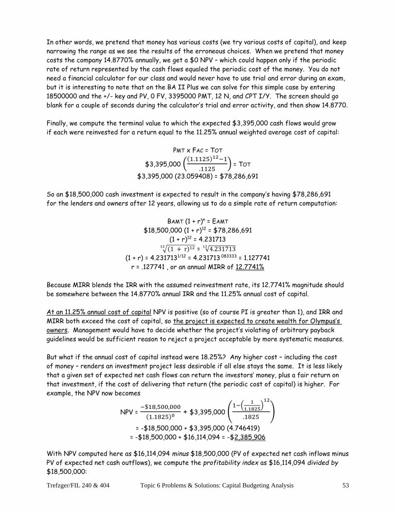
Trefzger/FIL 240 & 404 Topic 6 Problems & Solutions: Capital Budgeting Analysis 53
In other words, we pretend that money has various costs (we try various costs of capital), and keep
narrowing the range as we see the results of the erroneous choices. When we pretend that money
costs the company 14.8770% annually, we get a $0 NPV – which could happen only if the periodic
rate of return represented by the cash flows equaled the periodic cost of the money. You do not
need a financial calculator for our class and would never have to use trial and error during an exam,
but it is interesting to note that on the BA II Plus we can solve for this simple case by entering
18500000 and the +/- key and PV, 0 FV, 3395000 PMT, 12 N, and CPT I/Y. The screen should go
blank for a couple of seconds during the calculator’s trial and error activity, and then show 14.8770.
Finally, we compute the terminal value to which the expected $3,395,000 cash flows would grow
if each were reinvested for a return equal to the 11.25% annual weighted average cost of capital:
PMT x FAC = TOT
$3,395,000 ((1.1125)12−1
.1125) = TOT
$3,395,000 (23.059408) = $78,286,691
So an $18,500,000 cash investment is expected to result in the company’s having $78,286,691
for the lenders and owners after 12 years, allowing us to do a simple rate of return computation:
BAMT (1 + r)n = EAMT
$18,500,000 (1 + r)12 = $78,286,691
(1 + r)12 = 4.231713
√(1 + r)1212 = √4.23171312
(1 + r) = 4.2317131/12 = 4.231713.083333 = 1.127741
r = .127741 , or an annual MIRR of 12.7741%
Because MIRR blends the IRR with the assumed reinvestment rate, its 12.7741% magnitude should
be somewhere between the 14.8770% annual IRR and the 11.25% annual cost of capital.
At an 11.25% annual cost of capital NPV is positive (so of course PI is greater than 1), and IRR and
MIRR both exceed the cost of capital, so the project is expected to create wealth for Olympus’s
owners. Management would have to decide whether the project’s violating of arbitrary payback
guidelines would be sufficient reason to reject a project acceptable by more systematic measures.
But what if the annual cost of capital instead were 18.25%? Any higher cost – including the cost
of money – renders an investment project less desirable if all else stays the same. It is less likely
that a given set of expected net cash flows can return the investors’ money, plus a fair return on
that investment, if the cost of delivering that return (the periodic cost of capital) is higher. For
example, the NPV now becomes
NPV = −$18,500,000
(1.1825)0 + $3,395,000 (
1−(1
1.1825)
12
.1825)
= -$18,500,000 + $3,395,000 (4.746419)
= -$18,500,000 + $16,114,094 = -$2,385,906
With NPV computed here as $16,114,094 minus $18,500,000 (PV of expected net cash inflows minus
PV of expected net cash outflows), we compute the profitability index as $16,114,094 divided by
$18,500,000:
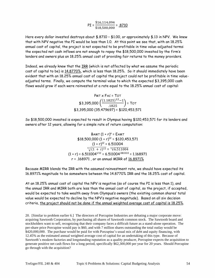
Trefzger/FIL 240 & 404 Topic 6 Problems & Solutions: Capital Budgeting Analysis 54
PI = $16,114,094
$18,500,000 = .8710
Here every dollar invested destroys about $.8710 – $1.00, or approximately $.13 in NPV. We knew
that with NPV negative the PI would be less than 1.0. At this point we see that, with an 18.25%
annual cost of capital, the project is not expected to be profitable in time value-adjusted terms:
the expected net cash inflows are not enough to repay the $18,500,000 invested by the firm’s
lenders and owners plus an 18.25% annual cost of providing fair returns to the money providers.
Indeed, we already knew that the IRR (which is not affected by what we assume the periodic
cost of capital to be) is 14.8770%, which is less than 18.25%. So it should immediately have been
evident that with an 18.25% annual cost of capital the project could not be profitable in time value-
adjusted terms. Finally, we compute the terminal value to which the expected $3,395,000 cash
flows would grow if each were reinvested at a rate equal to the 18.25% annual cost of capital:
PMT x FAC = TOT
$3,395,000 ((1.1825)12−1
.1825) = TOT
$3,395,000 (35.479697) = $120,453,571
So $18,500,000 invested is expected to result in Olympus having $120,453,571 for its lenders and
owners after 12 years, allowing for a simple rate of return computation:
BAMT (1 + r)n = EAMT
$18,500,000 (1 + r)12 = $120,453,571
(1 + r)12 = 6.511004
√(1 + r)1212 = √6.51100412
(1 + r) = 6.5110041/12 = 6.511004.083333 = 1.168971
r = .168971 , or an annual MIRR of 16.8971%
Because MIRR blends the IRR with the assumed reinvestment rate, we should have expected its
16.8971% magnitude to be somewhere between the 14.8770% IRR and the 18.25% cost of capital.
At an 18.25% annual cost of capital the NPV is negative (so of course the PI is less than 1), and
the annual IRR and MIRR both are less than the annual cost of capital, so the project, if accepted,
would be expected to take wealth away from Olympus’s owners (the existing common shares’ total
value would be expected to decline by the NPV’s negative magnitude). Based on all six decision
criteria, the project should not be done if the annual weighted average cost of capital is 18.25%.
20. [Similar to problem earlier 6.] The directors of Porcupine Industries are debating a major corporate move:
acquiring Sawtooth Corporation, by purchasing all shares of Sawtooth common stock. The Sawtooth board and
stockholders want to sell, recognizing that their company faces a difficult future as a stand-alone operation. The
per-share price Porcupine would pay is $60, and with 7 million shares outstanding the total outlay would be
$420,000,000. The purchase would be paid for with Porcupine’s usual mix of debt and equity financing, with
12.45% as the estimated annual weighted average cost of capital for an undertaking of this type. Because of
Sawtooth’s modern factories and longstanding reputation as a quality producer, Porcupine expects the acquisition to
generate positive net cash flows for a long period, specifically $62,300,000 per year for 20 years. Should Porcupine
go through with the acquisition?

Trefzger/FIL 240 & 404 Topic 6 Problems & Solutions: Capital Budgeting Analysis 55
Type: Evaluating Expansion Project with Equal Expected Cash Flows. Our systematic evaluation criteria
are the net present value (NPV), profitability index (PI), internal rate of return (IRR), and modified
internal rate of return (MIRR) methods. Foremost among them is NPV, the standard equation for
which is
NPV = CF0
(1 + r)0 +
CF1
(1 + r)1 +
CF2
(1 + r)2 +
CF3
(1 + r)3 + … +
CFn
(1 + r)n
= −$420,000,000
(1.1245)0 +
$62,300,000
(1.1245)1 +
$62,300,000
(1.1245)2 +
$62,300,000
(1.1245)3 + … +
$62,300,000
(1.1245)19 +
$62,300,000
(1.1245)20
With equal cash flows expected in years 1 through 20, we can get the same result with a shortened
form of the equation based on the PV of a level ordinary annuity factor for n = 20 periods:
NPV = −$420,000,000
(1.1245)0 + $62,300,000 (
1−(1
1.1245)
20
.1245)
= -$420,000,000 + $62,300,000 (7.263633)
= -$420,000,000 + $452,524,323 = $32,524,323
We compute the profitability index with the same two final values (PV of expected net cash inflows
and PV of expected net cash outflows) that determine NPV, but to find PI we compute not
$452,524,323 minus $420,000,000 but rather $452,524,323 divided by $420,000,000:
PI = $452,524,323
$420,000,000 = 1.0774
Because NPV is positive we know that the PI has to be greater than 1.0. And at this point we know
that the purchase is expected to be profitable in time value-adjusted terms: the expected net cash
inflows exceed the initial investment by enough to repay the Porcupine investors’ $420,000,000;
and also meet the 12.45% annual cost of providing fair returns to these lenders and owners; and
also increase the total value of the firm’s existing common stock by $32,524,323. The PI measure
tells us that every dollar invested generates about $.077 in NPV. And we also know that IRR should
exceed the 12.45% annual cost of capital; we compute it by solving for r in the equation
NPV = −$420,000,000
(1 + r)0 + $62,300,000 (
1−(1
1 + r)
20
r)
With trial and error we would find r, the IRR, to be 13.6945%; let’s double-check:
NPV = −$420,000,000
(1.136945)0 + $62,300,000 (
1−(1
1.136945)
20
.136945)
= -$420,000,000 + $62,300,000 (6.741587)
= -$420,000,000 + $420,000,000 = $0 ✓
(On an exam you would be expected to set up, or at lest recognize, the equation we would use in the
trial and error computations, but would not be asked to do the tedious trial and error computing.
The BA II Plus financial calculator, which we do not encourage you to use until you are sure that you

Trefzger/FIL 240 & 404 Topic 6 Problems & Solutions: Capital Budgeting Analysis 56
understand the underlying ideas, could do the trial & error for us: type 420000000 and the +/- key
and PV, 0 FV, 62300000 PMT, 20 N, CPT I/Y; the screen should go blank during the trial and error
attempts and then show 13.6945. Or in cash flow mode type CF 2nd CLR WORK 420000000 +/-
ENTER ↓, 62300000 ENTER ↓ 20 ENTER ↓ IRR CPT, the screen should go blank briefly and then
show 13.6945; then go ahead and type NPV 12.15 ENTER ↓ CPT, screen should quickly show the
$32,524,323 NPV we computed manually above.) In the trial and error process we pretend that
money has various costs (i.e., we try various costs of capital), and see which one results in a $0 NPV.
When we pretend money costs the company 13.6945% per year, we get a $0 NPV – which could
happen only if the return represented by the cash flows also were an annual 13.6945%.
Finally, we find the terminal value to which the expected $62,300,000 yearly cash flows would grow
if each were reinvested until the end of the project’s life at a rate equal to the 12.45% annual cost
of capital:
PMT x FAC = TOT
$62,300,000 ((1.1245)20−1
.1245) = TOT
$62,300,000 (75.917706) = $4,729,673,079
A $420,000,000 cash investment is expected to result in Porcupine’s having more than $4 billion
for its lenders and owners 20 years later. A simple rate of return computation shows these figures
to represent a compounded average annual rate of return (MIRR) of:
BAMT (1 + r)n = EAMT
$420,000,000 (1 + r)20 = $4,729,673,079
(1 + r)20 = 11.261126
√(1 + r)2020 = √11.26112620
(1 + r) = 11.2611261/20 = 11.261126.05 = 1.128701
r = .128701 , or an annual MIRR of 12.8701%
Here the 12.8701% annual MIRR is a blend of the 13.6945% annual IRR and the 12.45% annual cost
of capital (which we treat as the expected reinvestment rate in MIRR analysis).
In this case, with a positive NPV, PI exceeding 1, and IRR and MIRR both greater than the 12.45%
yearly cost of capital, the project is profitable in time value-adjusted terms. It is expected to give
the lenders and owners back their $420,000,000, plus returns to the lenders and owners that cost
the company 12.45% per year to deliver, and also increase the market value of the existing shares
of Porcupine common stock. The acquisition of Sawtooth would seem to be a good financial move.
21. [Similar to earlier problem 12.] After years of turning down snow removal jobs because of inadequate plowing
equipment, the managers of Mesabi Lawn & Lot have decided to buy ten top-quality Alpine Tyrannosaurus snow
plows. They are choosing from among three options:
Type Equipment Cost for Ten Expected Life Expected Annual Net Cash Flow
New $640,000 8 Years $175,000
Factory Reconditioned $384,000 4 Years $170,000
Used $205,000 2 Years $160,000
Expected annual cash flows are slightly lower for the reconditioned or used equipment due to higher expected
maintenance/repair costs. Because it plans to be in business indefinitely into the future, Mesabi will evaluate the
three possibilities based on a common 8-year investment period. Costs of reconditioned or used equipment, and

Trefzger/FIL 240 & 404 Topic 6 Problems & Solutions: Capital Budgeting Analysis 57
the net yearly cash flows from snow removal activities, are expected to remain largely unchanged over the next
eight years. Based on their experience, Mesabi managers feel that the resale value of any equipment at the end
of its expected life will be negligible. The company assigns a 14.25% annual cost of capital to all its equipment
purchases. Using the replacement chain method, determine which purchase option provides the highest net present
value (NPV). How does the equivalent annual annuity (EAA) method rank the three possibilities?
Type: Computing NPVs for Projects with Different Lives using Replacement Chain Approach. Here we compare
three competing projects with different expected lives. First we can compute the NPV for each
project separately:
NPVNew Equipment = −$640,000
(1.1425)0 + $175,000 (
1−(1
1.1425)
8
.1425)
= -$640,000 + $175,000 (4.600217) = -$640,000 + $805,038 = $165,038
NPVReconditioned Equipment = −$384,000
(1.1425)0 + $170,000 (
1−(1
1.1425)
4
.1425)
= -$384,000 + $170,000 (2.898843) = -$384,000 + $492,803 = $108,803
NPVUsed Equipment = −$205,000
(1.1425)0 + $160,000 (
1−(1
1.1425)
2
.1425)
= -$205,000 + $160,000 (1.641377) = -$205,000 + $262,620 = $57,620
If none of the projects were expected to be repeatable, the relevant comparison figure for each
would be the NPV value computed above, ranked as New Equipment best at a $165,038 NPV; then
reconditioned with a $108,803 NPV; and Used last with a $57,620 NPV. And with no expectation of
repeating any of the three, Mesabi would add the greatest possible amount to its owners’ wealth by
purchasing new equipment.
However, if Mesabi does not buy new plows it will want to keep reconditioned or used equipment in
operation for the same eight years that new models would be expected to last. Thus relevant NPV
comparison figures would have to involve eight years no matter what type of equipment the company
buys. We can use the replacement chain approach to compute combined NPVs over the eight-year
common time frame. We want to determine how much wealthier Mesabi’s owners would feel today
if the firm committed, today, to some means of having snow plowing equipment in place for the next
eight years. If it buys new plows, with their 8-year expected lives, the answer is the NPV of
$165,038 computed above.
If it opted for reconditioned plows, however, Mesabi would be expected to repeat this $108,803
NPV project at the end of year 4. The company’s owners would feel wealthier by $108,803 today,
and then we would expect them to feel richer again by $108,803 at the end of year 4, when a
new round of reconditioned plows would be procured to provide service in years 5 – 8. So we want
to measure how much wealthier they should feel today as a result of expecting to feel richer
by $108,803 twice: today and again in four years. We compute the latter value by discounting
$108,803 to a PV for the four periods expected to pass before the reconditioned equipment would
have to be replaced:
$108,803 (1
1.1425)
4
= $108,803 (.586915) = $63,858

Trefzger/FIL 240 & 404 Topic 6 Problems & Solutions: Capital Budgeting Analysis 58
The two together show the increase in wealth Mesabi’s owners would realize today from a decision
to purchase ten reconditioned plows today, and then buy ten reconditioned plows again 4 years
later, when the first reconditioned units need to be replaced:
NPVReconditioned Equipment Purchased Twice = $108,803 + $108,803 (1
1.1425)
4
= $108,803 + $63,858 = $172,661
Thus planning to plow with reconditioned equipment over the next 8 years adds more to the wealth
of Mesabi’s owners (the combined value of the existing common stock) than does buying new snow
plows. What about used equipment? If Mesabi bought used plows, it would expect to replace them
after two years, and then again every two subsequent years. So going with the used plows would
give Mesabi’s owners a $57,620 increase in wealth today. Then we would expect them to feel richer
again by $57,620 at the end of year 2, when ten “new” used plows are bought as replacements.
Then they would feel wealthier again by $57,620 at the ends of years 4 and 6. So how much richer
should these owners feel today as a result of their expectation of feeling richer by $57,620 in 2
years, and then by $57,620 again in 4 years, and then by $57,620 again in 6 years? Combining the
four, we compute:
NPVUsed Equip. Purch. 4 Times = $57,620 + $57,620 (1
1.1425)
2
+ $57,620(1
1.1425)
4+ $57,620(
1
1.1425)
6
= $57,620 + $44,143 +$33,818 + $25,908 = $161,489
If it is to be committed to having snow plowing equipment in place for eight years, the option that
adds the most to the owners’ wealth is buying the reconditioned equipment and replacing it after
4 years; that project offers the greatest ($172,661) contribution to the owners’ wealth. [If the
current owners of Mesabi were to sell all their common stock to a new group of owners, we would
expect the total price paid to be $172,661 more than it would have been before the managers had
committed to expanding their snow removal capabilities with the reconditioned plowing equipment.]
Buying new equipment has a lower NPV of $165,038, while used equipment has a combined NPV of
an even lower $161,489.
Another way to rank the projects would be with the equivalent annual annuity (EAA) method,
in which we annualize the NPV computed above for each project on a time value-adjusted basis.
New equipment’s $165,038 NPV annualized over an 8-year period is computed as:
PMT x FAC = TOT
PMT (1−(
1
1.1425)
8
.1425) = $165,038 so PMT (4.600217) = $165,038
PMT = $165,038 ÷ 4.600217 = $35,876.14 EAANew
Reconditioned equipment’s $108,803 NPV annualized over a 4-year period is computed as:
PMT x FAC = TOT
PMT (1−(
1
1.1425)
4
.1425) = $108,803 so PMT (2.898843) = $108,803
PMT = $108,803 ÷ 2.898843 = $37,533.26 EAAReconditioned

Trefzger/FIL 240 & 404 Topic 6 Problems & Solutions: Capital Budgeting Analysis 59
Finally, the used equipment’s $57,620 NPV annualized over a 2-year period is computed as:
PMT (1−(
1
1.1425)
2
.1425) = $57,620 so PMT (1.641377) = $57,620
PMT = $57,620 ÷ 1.641377 = $35,104.67 EAAUsed
We might think of EAA as the increase in wealth a project would continue to provide for the
firm’s owners every year if it were kept in ongoing operation. EAA should give the same ranking
as replacement chain: Reconditioned highest (EAA of $37,533.26); New second (EAA $35,876,14);
and Used last (EAA $35,104.67). An advantage of EAA analysis over replacement chain is that we
are not restricted to finding a common multiple of the various projects’ lives; with EAA we could
compare a 7-year project with a 9-year project without having to go out 7 x 9 = 63 years with our
cash flow estimates.
22. [Somewhat similar to earlier problem 8.] Andes Apparel is negotiating with Carpathian Cartoons for the rights
to produce children’s clothing featuring Carpathian character logos. Andes would pay $562,700 for licensing rights
to the cartoon figures for an 11-year period. If the internal rate of return (IRR) for the project is measured to be
13.25%, what additional net cash flow does Andes expect to generate each year by putting the Carpathian characters
on its products? If the cost of capital is 10.45% per year, what are the project’s modified internal rate of return
(MIRR) and net present value (NPV)? For how many years would that annual net cash flow have to persist to
provide Andes with an NPV of $150,000?
Type: Computing Cash Flows, MIRR, NPV, Number of Periods. Here the unknown we first solve for is the
extra net cash flow Andes expects to generate each year by having cartoon images on its children’s
wear. Recall that the IRR is the discount rate that causes the sum of the present values of all
expected net cash flows to be $0; thus:
$0 = −$562,700
(1.1325)0 + CF (
1−(1
1.1325)
11
.1325)
$0 = -$562,700 + CF (5.626893)
$562,700 = CF (5.626893)
CF = $562,700 ÷ 5.626893 = $100,002 ,
or about $100,000 per year. Now, knowing the expected stream of net cash flows and the annual
cost of capital (which we typically use as our reinvestment rate in MIRR analysis), we can compute
MIRR finding
PMT x FAC = TOT
$100,000 ((1.1045)11−1
.1045) = TOT
$100,000 (18.987231) = $1,898,723
as the terminal value, and then solving the simple rate of return problem:
BAMT (1+r)n = EAMT
$562,700 (1 + r)11 = $1,898,723
(1 +r)11 = 3.374308
√(1 + r)1111 = √3.37430811
(1 + r) = 3.3743081/11 = 3.374308.090909 = 1.116906
r = .116906 , or an annual MIRR of 11.6906%

Trefzger/FIL 240 & 404 Topic 6 Problems & Solutions: Capital Budgeting Analysis 60
(We should expect the 11.6906% annual MIRR to be between the 10.45% annual cost of capital and
the 13.25% annual IRR.) NPV based on a 10.45% annual weighted average cost of capital is simply
NPV = −$562,700
(1.1045)0 + $100,000 (
1−(1
1.1045)
11
.1045)
= –$562,700 + $100,000 (6.362660) = –$562,700 + $636,266 = $73,566
For the NPV instead to be a higher $150,000 the series of $100,000 net cash flows would have to
last for a longer time period:
$150,000 = −$562,700
(1.1045)0 + $100,000 (
1−(1
1.1045)
n
.1045) = – $562,700 + $100,000 (
1−(1
1.1045)
n
.1045)
$712,700 = $956,938[1 − (1
1.1045)
n]
$712,700 = $956,938 [1 − (. 905387)n]
$712,700 = $956,938 – $956,938 (.905837)n
$244,238 = $956,938 (.905837)n
.255229 = (.905837)n
ln .255229 = ln [(.905837)n]
ln .255229 = n ln .905837
-1.365595 = n (-.099393)
n = 13.739388 ,
or almost 14 years. Double-check:
−$562,700
(1.1045)0 + $100,000 (
1−(1
1.1045)
13.739388
.1045)
= – $562,700 + $100,000 (7.127000) =
= – $562,700 + $712,700 = $150,000 ✓
23. [FIL 404 only] Adirondack Music Stores is considering buying all the buildings and inventory (while taking
responsibility for the liabilities) of High Sierra Music Marts, a small but profitable family-owned chain whose
owners want to retire. The price that High Sierra’s owners are asking Adirondack to pay is $3,900,000.
Adirondack’s managers would expect the High Sierra locations to generate attractive net cash flows over an 18-year
period. The year 1 figure is expected to be $465,000, with subsequent years’ net cash flows expected to grow by
an average rate of 4% per year. Adirondack uses a 13.5% annual cost of capital assumption when evaluating store
acquisitions. Determine whether this project should be accepted, based on the net present value (NPV), profitability
index (PI), internal rate of return (IRR), and modified internal rate of return (MIRR) decision criteria.
Type: Evaluating Expansion Project with Changing Expected Cash Flows. The twist in this example is that
the cash flows are expected to change by a steady percentage from year to year. As always, we
start by computing NPV with the general equation
NPV = CF0
(1 + r)0 +
CF1
(1 + r)1 +
CF2
(1 + r)2 +
CF3
(1 + r)3 + … +
CFn
(1 + r)n
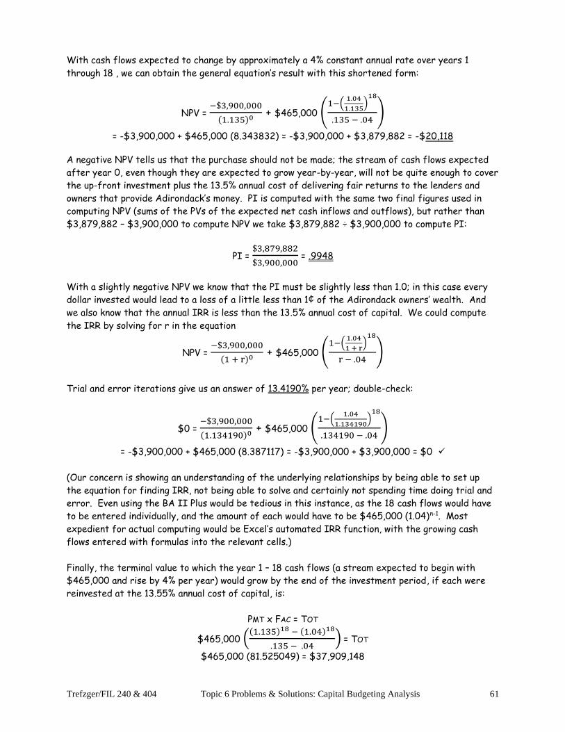
Trefzger/FIL 240 & 404 Topic 6 Problems & Solutions: Capital Budgeting Analysis 61
With cash flows expected to change by approximately a 4% constant annual rate over years 1
through 18 , we can obtain the general equation’s result with this shortened form:
NPV = −$3,900,000
(1.135)0 + $465,000 (
1−(1.04
1.135)
18
.135 − .04)
= -$3,900,000 + $465,000 (8.343832) = -$3,900,000 + $3,879,882 = -$20,118
A negative NPV tells us that the purchase should not be made; the stream of cash flows expected
after year 0, even though they are expected to grow year-by-year, will not be quite enough to cover
the up-front investment plus the 13.5% annual cost of delivering fair returns to the lenders and
owners that provide Adirondack’s money. PI is computed with the same two final figures used in
computing NPV (sums of the PVs of the expected net cash inflows and outflows), but rather than
$3,879,882 – $3,900,000 to compute NPV we take $3,879,882 ÷ $3,900,000 to compute PI:
PI = $3,879,882
$3,900,000 = .9948
With a slightly negative NPV we know that the PI must be slightly less than 1.0; in this case every
dollar invested would lead to a loss of a little less than 1¢ of the Adirondack owners’ wealth. And
we also know that the annual IRR is less than the 13.5% annual cost of capital. We could compute
the IRR by solving for r in the equation
NPV = −$3,900,000
(1 + r)0 + $465,000 (
1−(1.04
1 + r)
18
r − .04)
Trial and error iterations give us an answer of 13.4190% per year; double-check:
$0 = −$3,900,000
(1.134190)0 + $465,000 (
1−(1.04
1.134190)
18
.134190 − .04)
= -$3,900,000 + $465,000 (8.387117) = -$3,900,000 + $3,900,000 = $0 ✓
(Our concern is showing an understanding of the underlying relationships by being able to set up
the equation for finding IRR, not being able to solve and certainly not spending time doing trial and
error. Even using the BA II Plus would be tedious in this instance, as the 18 cash flows would have
to be entered individually, and the amount of each would have to be $465,000 (1.04)n-1. Most
expedient for actual computing would be Excel’s automated IRR function, with the growing cash
flows entered with formulas into the relevant cells.)
Finally, the terminal value to which the year 1 – 18 cash flows (a stream expected to begin with
$465,000 and rise by 4% per year) would grow by the end of the investment period, if each were
reinvested at the 13.55% annual cost of capital, is:
PMT x FAC = TOT
$465,000 ((1.135)18 − (1.04)18
.135 − .04) = TOT
$465,000 (81.525049) = $37,909,148

Trefzger/FIL 240 & 404 Topic 6 Problems & Solutions: Capital Budgeting Analysis 62
A $3,900,000 cash investment is expected to result in Adirondack’s having $37,909,148 for its
lenders and owners after 18 years. We then compute the indicated MIRR as a simple rate of return
computation:
BAMT (1 + r)n = EAMT
$3,900,000 (1 + r)18 = $37,909,148
(1 + r)18 = 9.720294
√(1 + r)1818 = √9.72029418
(1 + r) = 9.7202941/18 = 9.720294.055556 = 1.134674
r = .134674 , or an annual MIRR of 13.4674%
Here the 13.4674% annual MIRR is a blend of the 13.4190% annual IRR and the 13.5% annual cost
of capital that is treated as the expected reinvestment rate in MIRR analysis.
In this case, with a slightly negative NPV, PI less than 1, and annual IRR and MIRR percentages
both slightly less than the 13.5% annual cost of capital, Adirondack should not complete the
purchase of High Sierras’ assets. Doing so would not be profitable in time value-adjusted terms;
the company would not generate enough in cash flows (despite the expected growth in the receipts)
to recoup the $3,900,000 investment plus the 13.5% annual percentage cost of providing fair
returns to the company’s money providers. The investment would make sense only if the sellers of
High Sierras would accept an offering price of $3,879,882 (or less); that price would result in an
NPV of $3,879,882 - $3,879,882 = $0, which is the minimum acceptable NPV for an investment
project. ●