Tests of the CAPM and the

Fama-French Methodology

1

Testing the CAPM: The Basics

• The most commonly quoted equation for the CAPM is

E (Ri ) = Rf + βi [E (Rm)− Rf ]

• So the CAPM states that the expected return on any stock i isequal to the risk-free rate of interest, Rf , plus a risk premium.

• This risk premium is equal to the risk premium per unit ofrisk, also known as the market risk premium, [E (Rm)− Rf ],multiplied by the measure of how risky the stock is, known as‘beta’, βi

• Beta is not observable from the market and must becalculated, and hence tests of the CAPM are usually done intwo steps:

– Estimating the stock betas– Actually testing the model

• If the CAPM is a good model, then it should hold ’onaverage’.

2

Testing the CAPM: Calculating Betas

• A stock’s beta can be calculated in two ways:

1. Calculate it directly as the covariance between the stock’sexcess return and the excess return on the market portfolio,divided by the variance of the excess returns on the marketportfolio:

βi =Cov(Re

i ,Rem)

Var(Rem)

where the e superscript denotes excess return

2. Equivalently, we can run a simple time-series regression of theexcess stock returns on the excess returns to the marketportfolio separately for each stock, and the slope estimate willbe the beta:

Rei ,t = αi + βiR

em,t + ui ,t

3

Testing the CAPM: The Second Stage Regression

• Example:

• Suppose that we had a sample of 100 stocks (N=100) andtheir returns using five years of monthly data (T=60)

• The first step would be to run 100 time-series regressions (onefor each individual stock), the regressions being run with the60 monthly data points

• The second stage involves a single cross-sectional regressionof the average (over time) of the stock returns on a constantand the betas:

R̄i = λ0 + λ1βi + vi

where R̄i is the return for stock i averaged over the 60 months

4

Testing the CAPM: The Second Stage Regression(Cont’d)

• Essentially, the CAPM says that stocks with higher betas aremore risky and therefore should command higher averagereturns to compensate investors for that risk

• If the CAPM is a valid model, two key predictions arise whichcan be tested using this second stage regression:

1. λ0 = Rf ;

2. λ1 = [Rm − Rf ].

5

Testing the CAPM: Further Implications

• Two further implications of the CAPM being valid:– There is a linear relationship between a stock’s return and its

beta– No other variables should help to explain the cross-sectional

variation in returns

• We could run the augmented regression:

R̄i = λ0 + λ1βi + λ2β2i + λ3σ

2i + vi

where β2i is the squared beta for stock i and σ2

i is the varianceof the residuals from the first stage regression, a measure ofidiosyncratic risk

• The squared beta can capture non-linearities in therelationship between systematic risk and return

• If the CAPM is a valid and complete model, then we shouldsee that λ2 = 0 and λ3 = 0.

6

Testing the CAPM: A Different Second-StageRegression

• It has been found that returns are systematically higher forsmall capitalisation stocks and are systematically higher for‘value’ stocks than the CAPM would predict.

• We can test this directly using a different augmented secondstage regression:

R̄i = α+ λ1βi + λ2MVi + λ3BTMi + vi

where MVi is the market capitalisation for stock i and BTMi

is the ratio of its book value to its market value of equity

• Again, if the CAPM is a valid and complete model, then weshould see that λ2 = 0 and λ3 = 0.

7

Problems in Testing the CAPM

• Problems are numerous, and include:

– Heteroscedasticity – some recent research has used GMM oranother robust technique to deal with this

– Measurement errors since the betas used as explanatoryvariables in the second stage are estimated – in order tominimise such measurement errors, the beta estimates can bebased on portfolios rather than individual securities

8

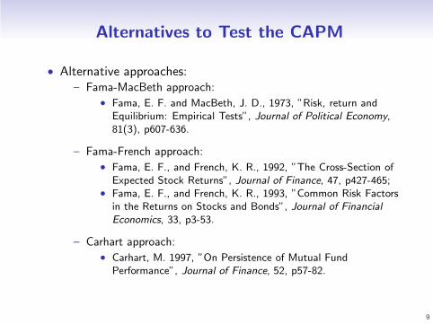
Alternatives to Test the CAPM

• Alternative approaches:– Fama-MacBeth approach:

• Fama, E. F. and MacBeth, J. D., 1973, ”Risk, return andEquilibrium: Empirical Tests”, Journal of Political Economy,81(3), p607-636.

– Fama-French approach:

• Fama, E. F., and French, K. R., 1992, ”The Cross-Section ofExpected Stock Returns”, Journal of Finance, 47, p427-465;

• Fama, E. F., and French, K. R., 1993, ”Common Risk Factorsin the Returns on Stocks and Bonds”, Journal of FinancialEconomics, 33, p3-53.

– Carhart approach:

• Carhart, M. 1997, ”On Persistence of Mutual FundPerformance”, Journal of Finance, 52, p57-82.

9

The Fama-MacBeth Approach

• Fama and MacBeth (1973) used the two stage approach totesting the CAPM outlined above, but using a time series ofcross-sections

• Instead of running a single time-series regression for eachstock and then a single cross-sectional one, the estimation isconducted with a rolling window

• They use five years of observations to estimate the CAPMbetas and the other risk measures (the standard deviation andsquared beta) and these are used as the explanatory variablesin a set of cross-sectional regressions each month for thefollowing four years

10

The Fama-MacBeth Approach (Cont’d)• The estimation is then rolled forward four years and theprocess continues until the end of the sample is reached

• Since we will have one estimate of the lambdas for each timeperiod, we can form a t-ratio as the average over t divided byits standard error (the standard deviation over time divided bythe square root of the number of time-series estimates of thelambdas).

• The average value of each lambda over t can be calculatedusing:

λ̂j =1

TFMB

TFMB∑

t=1

λ̂j ,t , j = 1, 2, 3, 4

where TFMB is the number of cross-sectional regressions usedin the second stage of the test, the j are the four different

11

The Fama-MacBeth Approach (Cont’d)

parameters (the intercept, the coefficient on beta, etc.) andthe standard deviation is

σ̂j =

√

√

√

√

1

TFMB − 1

TFMB∑

t=1

(λ̂j ,t − λ̂j)2

• The test statistic is then simply√TFMB λ̂j/σ̂j , which is

asymptotically standard normal, or follows a t-distributionwith TFMB − 1 degrees of freedom in finite samples.

12

The Fama-French Methodology

• The ‘Fama-French methodology’ is a family of relatedapproaches based on the notion that market risk is insufficientto explain the cross-section of stock returns

• The Fama-French and Carhart models seek to measureabnormal returns after allowing for the impact of thecharacteristics of the firms or portfolios under consideration

• It is widely believed that small stocks, value stocks, andmomentum stocks, outperform the market as a whole

• If we wanted to evaluate the performance of a fund manager,it would be important to take the characteristics of theseportfolios into account to avoid incorrectly labelling amanager as having stock-picking skills.

13

The Fama-French (1992) Approach• The Fama-French (1992) approach, like Fama and MacBeth(1973), is based on a time-series of cross-sections model

• A set of cross-sectional regressions are run of the form

Ri ,t = α0,t + α1,tβi ,t + α2,tMVi ,t + α3,tBTMi ,t + ui ,t

where Ri ,t are again the monthly returns, βi ,t are the CAPMbetas, MVi ,t are the market capitalisations, and BTMi ,t arethe book-to-price ratios, each for firm i and month t

• So the explanatory variables in the regressions are the firmcharacteristics themselves

• Fama and French show that size and book-to-market arehighly significantly related to returns

• They also show that market beta is not significant in theregression (and has the wrong sign), providing very strongevidence against the CAPM.

14

The Fama-French (1993) Approach

• Fama and French (1993) use a factor-based model in thecontext of a time-series regression which is run separately oneach portfolio i

Ri ,t = αi + βi ,MRMRFt + βi ,SSMBt + βi ,VHMLt + ǫi ,t

where R i,t is the return on stock or portfolio i at time t,RMRF, SMB, and HML are the factor mimicking portfolioreturns for market excess returns, firm size, and valuerespectively

• The excess market return is measured as the difference inreturns between the S&P 500 index and the yield on Treasurybills (RMRF)

15

The Fama-French (1993) Approach (Cont’d)

• SMB is the difference in returns between a portfolio of smallstocks and a portfolio of large stocks, termed ‘Small MinusBig

• HML is the difference in returns between a portfolio of valuestocks and a portfolio of growth stocks, termed ‘High MinusLow’.

• Check Ken French webpage for more details on the”Fama-French factors”.

16

The Fama-French (1993) Approach 2

• These time-series regressions are run on portfolios of stocksthat have been two-way sorted according to theirbook-to-market ratios and their market capitalisations

• It is then possible to compare the parameter estimatesqualitatively across the portfolios i

• The parameter estimates from these time-series regressionsare factor loadings that measure the sensitivity of eachindividual portfolio to the factors

• The second stage in this approach is to use the factor loadingsfrom the first stage as explanatory variables in across-sectional regression:

R̄i = α+ λMβi ,M + λSβi ,S + λVβi ,V + ei

17

The Fama-French (1993) Approach 2 (Cont’d)

• We can interpret the second stage regression parameters asfactor risk premia that show the amount of extra returngenerated from taking on an additional unit of that source ofrisk.

18

The Carhart (1997) Approach

• It has become customary to add a fourth factor to theequations above based on momentum

• This is measured as the difference between the returns on thebest performing stocks over the past year and the worstperforming stocks – this factor is known as UMD –‘up-minus-down’

• The first and second stage regressions then becomerespectively:

Ri ,t = αi + βi ,MRMRFt + βi ,SSMBt + βi ,VHMLt

+βi ,UUMDt + ǫi ,t

R̄i = α+ λMβi ,M + λSβi ,S + λVβi ,V + λUβi ,U + ei

19

The Carhart (1997) Approach (Cont’d)

• Carhart forms decile portfolios of mutual funds based on theirone-year lagged performance and runs the time-seriesregression on each of them

• He finds that the mutual funds which performed best last year(in the top decile) also had positive exposure to themomentum factor (UMD) while those which performed worsthad negative exposure.

20

More recently

• Researchers develop their own factors:

• Lettau and Ludvigson’s (2001) conditional version of theconsumption CAPM (CC-CAY);

• Lustig and Van Nieuwerburgh’s (2005) conditional version ofthe consumption CAPM (CC-MY);

• Santos and Veronesi’s (2006) conditional version of the CAPM(C-SW);

• Li, Vassalou, and Xing’s (2006) investment growth model(IGM);

• Petkova’s (2006) empirical implementation of Merton’s (1973)intertemporal extension of the CAPM (ICAPM) based onCampbell (1996);

• Yogo’s (2006) (D-CCAPM) is due to and highlights thecyclical role of durable consumption in asset pricing;

• · · ·

21

More recently (Cont’d)

Model Number of factors List of factors

CC-CAY 4 1, cayt−1, cnd,t , cnd,t · cayt−1

CC-MY 4 1, myt−1, cnd,t , cnd,t ·myt−1

C-SW 3 1, rmkt,t , rmkt,t · swt−1

IGM 6 1, ihh,t , icorp,t , incorp,t , ifcorp,t , ifm,t

ICAPM 6 1, rmkt,t , termt , deft , divt , rftCCAPM 4 1, rmkt,t , cnd,t , cd,t

22

Description of the factors:cnd growth rate in real per capita nondurable consumption (seasonally adjusted at annual rates) from BEAcay consumption-aggregate wealth ratio of Lettau and Ludvigson (2001) from Martin Lettau’s websitemy housing collateral ratiormkt excess return (in excess of the one-month T-bill rate) on the value-weighted stock market index

(NYSE-AMEX-NASDAQ) from Kenneth French’s websitesw labor income-consumption ratioihh log (gross fixed) investment growth rates for householdsicorp log (gross fixed) investment growth rates for non-financial corporationsincorp log (gross fixed) investment growth rates for non-corporate sectorifcorp log (gross fixed) investment growth rates for financial corporationsifm log (gross fixed) investment growth rates for farm sectorterm difference between the yields of ten-year and one-year government bonds (from the Board

of Governors of the Federal Reserve System)def difference between the yields of long-term corporate Baa bonds (from the Board of

Governors of the Federal Reserve System) and long-term government bonds (from Ibbotson Associates)div dividend yield on the Center for Research in Security Prices (CRSP) value-weighted stock market portfoliorf one-month T-bill yield (from CRSP, Fama Risk Free Rates)cd growth rate in real per capita durable consumption (seasonally adjusted at annual rates) from BEA

• New econometric issues arise:• identification• misspecification• · · ·

23