Capacity Analysis of the Union Station Rail Corridor using...
78
Capacity Analysis of the Union Station Rail Corridor using Integrated Rail and Pedestrian Simulation Yishu Pu MASc Student Department of Civil Engineering University of Toronto
Transcript of Capacity Analysis of the Union Station Rail Corridor using...
Capacity Analysis of the Union Station Rail Corridor using Integrated Rail and Pedestrian Simulation
Yishu PuMASc Student
Department of Civil Engineering
University of Toronto

Presentation Outline
Introduction
Railway Capacity Approaches
Toronto Union Station Rail Corridor
Data
Analytical Capacity Methods
Railway Simulation
Integrated Rail and Pedestrian Simulation – Nexus
Scenario Tests and Results
Conclusion
2

Introduction
3
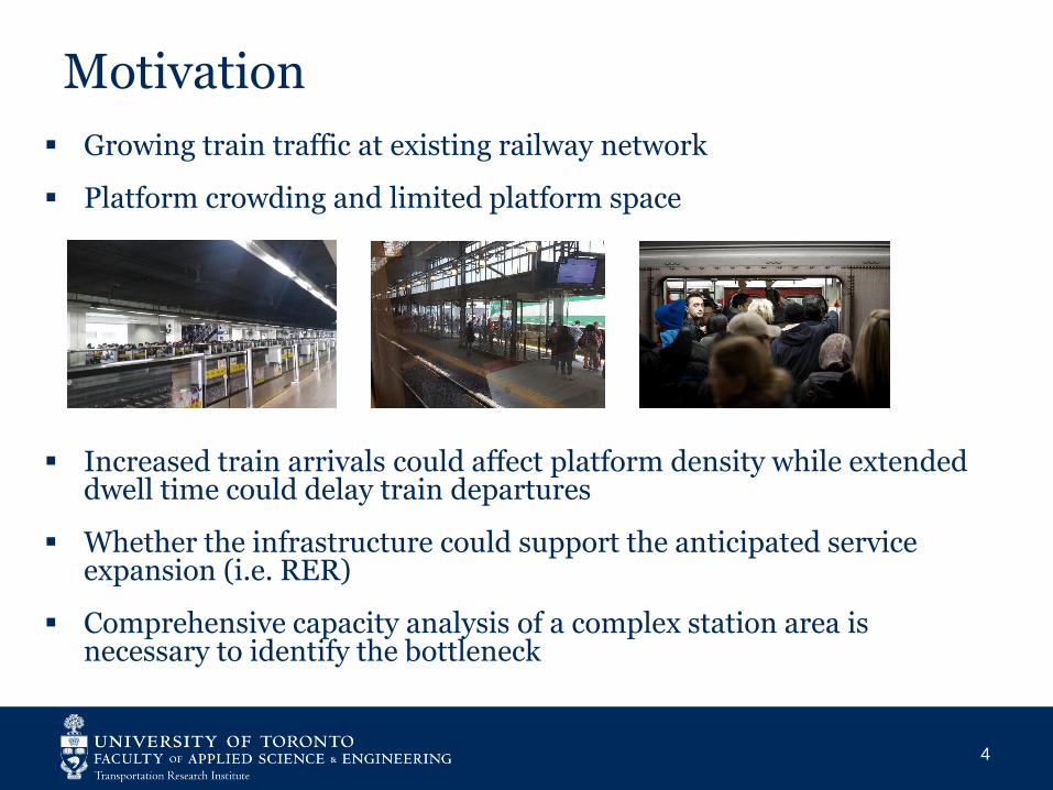
Motivation
Growing train traffic at existing railway network
Platform crowding and limited platform space
Increased train arrivals could affect platform density while extended dwell time could delay train departures
Whether the infrastructure could support the anticipated service expansion (i.e. RER)
Comprehensive capacity analysis of a complex station area is necessary to identify the bottleneck
4

Railway Capacity Approaches
5

6
Railway Passenger
Maximum number of trains
for a specified time period
over a defined section/area
under certain service quality
Maximum number of passengers
for a specified time period
over a defined section/area
under certain service quality
Railway System Capacity

Railway Capacity
Problem:– Results could vary largely due to different assumptions– Few studies compared methods in different categories– Virtually all dwell time is fixed (TCQSM, 2013)
Article Name Author Year Type
An analytical approach for the analysis of railway nodes
extending the Schwanhäußer’s method to railway stations and
junctions
De Kort et al. 1999
UIC Code 406 1st edition International Union of Railways 2004
Techniques for absolute capacity determination in railways Burdett and Kozan 2006
Development of Base Train Equivalents to Standardize Trains
for Capacity AnalysisLai et al. 2012
Transit Capacity and Quality of Service Manual Kittelson & Associates, Inc. et al. 2013
A synthetic approach to the evaluation of the carrying capacity
of complex railway nodeMalavasi et al. 2014
A Model, Algorithms and Strategy for Train Pathing Carey & Lockwood 1995
Optimal scheduling of trains on a single line track Higgins et al. 1996
A Job-Shop Scheduling Model for the Single-Track Railway
Scheduling ProblemOliveira and Smith 2000
UIC Code 406 2nd edition International Union of Railways 2013
An assessment of railway capacity Abril et al. 2008
US & USRC Track Capacity Study AECOM 2011
Evaluation of ETCS on railway capacity in congested area : a
case study within the network of Stockholm: A case study within
the network of Stockholm
Nelladal et al. 2011
Simulation Study Based on OpenTrack on Carrying Capacity in
District of Beijing-Shanghai High-Speed RailwayChen and Han 2014
Railway capacity analysis: methods for simulation and evaluation
of timetables, delays and infrastructureLindfeldt 2015
Analytical
Optimization
Simulation
7

Platform
Pedestrian Movements
Traditional dwell time modeling– Boarding/Alighting/Through passengers,
Regression models (San & Masirin, 2016)
Pedestrian Modelling– Analytical modelling– Simulation
Problem– Traditional dwell time models can not show
the platform density, or reflect the flow complication due to infrastructure layout
– Transit vehicle arrival/departure time is fixed
8
Train CarArticle Name Author Year Simulation
Pedestrian planning and design Fruin 1971
Social force model for pedestrian dynamics Helbing & Molnár 1995
The Flow of Human Crowds Hughes 2003
Autonomous Pedestrians Shao and Terzopoulos 2007
Pedestrian Simulation Research of Subway
Station in Special EventsZhao et al. 2009 Legion
Using Simulation to Analyze Crowd Congestion
and Mitigation at Canadian Subway
Interchanges
King et al. 2014 MassMotion
Use of Agent-Based Crowd Simulation to
Investigate the Performance of Large-Scale
Intermodal Facilities
Hoy et al. 2016 MassMotion

Integrated Simulation
Key assumptions for individual simulators:
– Fixed dwell time
– Fixed train arrival/departure time
Current models:
– Rail simulation with mathematical dwell time model (Jiang et al., 2015) (D’Acierno et al., 2017)
– Rail simulation with pedestrian simulation model (Srikukenthiran & Shalaby, 2017)
9

Problem Statement
Few studies compared methods in different categories
Interactive effects of pedestrian and train movements are not well captured by individual simulator
Train
Movements
Passenger
Movements
?
10

Study approach
Analytical Capacity Analysis(TCQSM, Potthoff method, DB method, Compression method)
Railway SimulationOpenTrack
Railway and Pedestrian SimulationNexus Platform – OpenTrack and MassMotion
11

Case Study - Toronto Union Station Rail Corridor (USRC)
12

Union Station Rail Corridor (USRC)
Built and opened in 1927 760,000 square feet of total floor space 14 track depots, 23 platforms, 350m long and 5m wide on average Toronto’s transportation hub for GO Transit, VIA Rail and UP
Express; as well as TTC Canada’s busiest transportation facility: 200,000 passengers pass
through Union Station on most business day
13
155,000 GO Train passengers and 10,000 bus passengers on a typical business day
208 daily GO Train trips
43 million annual passengers for GO train and bus
20 million annual passengers for TTC
2.4 million annual passengers for VIA

Scope
Study time period: 8am to 9am
One station away on any rail service
Assume unlimited capacity at yards and through movements at the station
Focus on maximum number of GO train trips during peak hour
14

Data
15

Required Data
Infrastructure data– Track layout– Signal location– Station layout
Operational data– Speed limit– Train profile and configuration– Schedule– Delay data– Ridership– Passenger flow
16

Manual Data Collection
Train Speed (GPS) Commonly-used Train Path Identification (Video
Recording) Entry Delay at prior stations and Arrival Delay at Union
Station (gotracker.ca)
17

Manual Data Collection
Platform Staircase Passenger Volume Count
Passenger Flow Count at Train Door
Dwell Time
18

Analytical Capacity Methods
19

Analytical Methods
– Transit Capacity and Quality of Service Manual (TCQSM)
– Potthoff method
– Deutsche Bahn (DB) method
– UIC Compression Method
20

TCQSM
Min. headway at Mainline– minimum train separation + operating margin
𝑡𝑐𝑠 =2(𝐿𝑡 + 𝑑𝑒𝑏)
𝑎 + 𝑎𝑔𝐺0+𝐿𝑡𝑣𝑎
+1
𝑓𝑏𝑟+ 𝑏
𝑣𝑎
2 𝑑 + 𝑎𝑔𝐺𝑖+
𝑎 + 𝑎𝑔𝐺0 𝑙𝑣2𝑡𝑜𝑠
2
2𝑣𝑎1 −
𝑣𝑎𝑣𝑚𝑎𝑥
+ 𝑡𝑜𝑠 + 𝑡𝑗𝑙 + 𝑡𝑏𝑟
ℎ𝑛𝑖 = 𝑡𝑐𝑠 + 𝑡𝑜𝑚
Min. headway at Station Area
– minimum train separation + critical station dwell time + operating marginℎ𝑛𝑖 = 𝑡𝑐𝑠 + 𝑡𝑑,𝑐𝑟𝑖𝑡 + 𝑡𝑜𝑚
Min. headway at Mainline with switches– if a train is encountered with a switch blocking when traveling at main line
ℎ𝑗 = 𝑡𝑐𝑠 +2(𝐿𝑡 + 𝑛 ∙ 𝑓𝑠𝑎𝑑𝑡𝑠)
𝑎+𝑣𝑚𝑎𝑥
𝑎 + 𝑑+ 𝑡𝑠𝑤 + 𝑡𝑜𝑚
21

TCQSM
TCQSM – Detailed calculation for line capacity, simple junction capacity calculation
Need for methods calculating node capacity
Station Area East Ladders/InterlockingWest Ladders/InterlockingW. M. Line E. M. Line
22

Potthoff method and Deutsche Bahn (DB) method
Assume trains could arrive at any instant of an assigned time period with the same probability
Timetable not required
Input:
• Identify all possible train paths in a system
• Summarize number of movements concerning each path (𝑛𝑖)
• Matrix of occupancy time for conflicting movements (𝑡𝑖𝑗)
• Priority Matrix (DB method, Optional)
Path 1-I 1-II 1-IV 4-III 4-IV III-2 IV-2 I-3 II-3 IV-3
# of movements 56 55 7 112 8 112 8 56 55 7
Path 1-I 1-II 1-IV 4-III 4-IV III-2 IV-2 I-3 II-3 IV-3
1-I 3.8 1.55 0.97 0 0 0 0 0 0 0
1-II 0.9 1.95 0.61 0 0 0 0 0 0 0
1-IV 1.45 1.45 4.03 0 4.21 1.47 0 0 0 0
4-III 0 0 0 1.67 0.61 0 0 0 0 0.61
4-IV 0 0 3.7 1.54 3.44 0 0 0 0 0
III-2 0 0 1.22 1.06 0 1.56 1.56 0 0 0
IV-2 0 0 2.16 0 1.9 2.93 2.93 0 0 0
I-3 2.74 0 0 0 0 0 0 3.17 3.17 3.17
II-3 0 1.2 0 0 0 0 0 1.54 1.54 1.54
IV-3 0 0 2.56 2.74 2.74 0 0 3.17 3.17 3.17

Capacity indicator
Potthoff method𝐵+𝑅
𝑇≤ 1 (𝑜𝑣𝑒𝑟 𝑐𝑎𝑝𝑎𝑐𝑖𝑡𝑦 𝑖𝑓 𝑏𝑖𝑔𝑔𝑒𝑟 𝑡ℎ𝑎𝑛 1)
𝐵: Total time of occupation
𝑅: Average delay
𝑇: Study period
Deutsche Bahn (DB) method𝐿𝑧 =
𝑘 ∙ 𝑃𝑏 ∙ 𝑥2
𝑇 − 𝑥 ∙ 𝐵𝑢𝑠𝑢𝑎𝑙𝑙𝑦 = 0.6 ;
𝑥 ≥ 1 (𝑜𝑣𝑒𝑟 𝑐𝑎𝑝𝑎𝑐𝑖𝑡𝑦 𝑖𝑓 𝑠𝑚𝑎𝑙𝑙𝑒𝑟 𝑡ℎ𝑎𝑛 1)
𝐿𝑧 : average number of trains in the waiting queue (to evaluate operation quality)
𝑘: Probability with which the movements relating to the complex node are mutually exclusive
𝑃𝑏: Occupancy time considering priority
𝑥: Scale factor

Union Station Case
Two complex interlocking areas located at west and east of the station
Possible combination of routes could add up to 4000
30 and 24 identified commonly used train paths for west interlocking and east interlocking areas respectively
Train paths shared by GO trains, VIA rail trains, and UP Express trains
Some paths might be affected by the station dwell time

Matrices of occupancy time for conflicting movements
Path # - Excluded 1 2 3 4 5 6 7 8 9 10 11 12 13 14 15 16 17 18 19 20 21 22 23 24 25 26 27 28 29 30
Path # - Actual (min) D2-SL2-UD14 D2-SL2-UD13 D1-SL2-UD13 D1-SL2-UD14 C2-NL2-UD12 C2-NL2-UD7 A1-NL2-UD7 C1-NL2-UD12 C1-NL2-UD7 C1-SL2-UD12 C2-SL2-UD12 C1-SL1-UD4 C1-NL2-UD6 A1-NL1-UPXS C2-NL1-UPXS UPXS-NL1-B D1-NL2-UD11 D1-NL2-UD10 UD11-NL2-A3 UD10-NL2-A3 UD2-SL1-NL1-B UD2-SL1-A2 UD1-NL1-A2 UD1-NL1-B UD3-SL1-A2 UD3-SL1-A2-NL2-B UD4-SL1-NL1-A2 UD4-A2-NL2-B UD5-A3-NL2-B UD5-A3-NL2-A2
1 D2-SL2-UD14 6.5 2 2 6.5 2 2
2 D2-SL2-UD13 2 6.5 6.5 2 3 3 2 2
3 D1-SL2-UD13 2 6.5 6.5 2 3 3 2 2 1.5 1.5
4 D1-SL2-UD14 6.5 2 2 6.5 2 2 1.5 1.5
5 C2-NL2-UD12 2 2 6.5 2 2 6.5 1.5 7 7 1.5 1.5 2 2 2.5 2.5
6 C2-NL2-UD7 2 6.5 6.5 2 6.5 1.5 1.5 1.5 1.5 2 2 1.5 1.5
7 A1-NL2-UD7 2 7 6.5 2 7 1.5 1.5 1.5 2 2 2 2 2 0 0 0 0 0 0 0 0
8 C1-NL2-UD12 2 2 6.5 2 2 6.5 1.5 7 7 1.5 1.5 1.5 2 2 2.5 2.5
9 C1-NL2-UD7 2 6.5 6.5 2 6.5 1.5 1.5 1.5 1.5 2 2 1.5 1.5
10 C1-SL2-UD12 2 2 2 2 6.5 1.5 6.5 1.5 6.5 6.5 1.5 1.5 1.5 1.5 1.5
11 C2-SL2-UD12 1.5 2 2 1.5 6.5 1.5 6.5 6.5 6.5 1.5 1.5 1.5
12 C1-SL1-UD4 1.5 1.5 1.5 1.5 7.5 1.5 2 1 1 2.5 2 2 8.5 8.5 1.5 1.5
13 C1-NL2-UD6 1.5 1.5 1.5 1.5 1.5 1.5 1.5 6.5 1.5 1.5 1.5
14 A1-NL1-UPXS 1 6 6 6 2 6 6 2 0 0
15 C2-NL1-UPXS 1 1 1 1 1 1 1 1 1 6 6 7 0.5 0.5 1.5 1.5 7 7 1.5 1.5 0.5 0.5 0.5 0.5
16 UPXS-NL1-B 0 1 1.5 1 0.5 1 0 0 0
17 D1-NL2-UD11 1.5 1.5 2 2 2 2 2 1.5 1.5 23 2 23 2.5
18 D1-NL2-UD10 1.5 1.5 2 2 2 2 2 1.5 1.5 2 23 2.5 23
19 UD11-NL2-A3 2.5 2.5 2.5 2.5 2 2 2 2.5 2.5 2.5 1.5 1.5 0.5 0.5
20 UD10-NL2-A3 2.5 2.5 2.5 2.5 2 2 2 2.5 2.5 2.5 1.5 1.5 0.5 0.5
21 UD2-SL1-NL1-B 1 2 2.5 2.5 1.5 1.5 2.5 1.5 0.5 1
22 UD2-SL1-A2 0 1.5 2.5 1.5 2 2 2 2 2 2 1 1
23 UD1-NL1-A2 2.5 1 2.5 2 2 1.5 2 2 2 2 1.5 1.5 0.5 0.5
24 UD1-NL1-B 0 1 1.5 1.5 1 1.5 0.5 0.5 0.5 0
25 UD3-SL1-A2 0 1.5 2.5 2 2 2 2 2 2 1 1
26 UD3-SL1-A2-NL2-B 0 1.5 2.5 2.5 2 1.5 2 2 2 2 2 2 2 1 1
27 UD4-SL1-NL1-A2 0 1.5 2.5 2 2 2 2 2 2 1 1
28 UD4-A2-NL2-B 0 1.5 0 2.5 0 1.5 2 3 2 2 2 2 2 1 1
29 UD5-A3-NL2-B 0 1.5 0 2.5 2 2.5 2.5 1.5 1 1 1.5 1 1 1 1 2 2
30 UD5-A3-NL2-A2 0 1.5 2.5 2 2 1 1 0 0 0.5 0.5 2 2
Path # - Excluded 1 2 3 4 5 6 7 8 9 10 11 12 13 14 15 16 17 18 19 20 21 22 23 24
Path # - Actual (min) E1-NL1-UD3 E1-NL1-UD4 E1-NL1-UD2 E1-NL1-UD1 E2-NL1-UD3 E4-NL1-UD3 E3-NL1-UD3 E3-NL1-UD5 E3-NL1-UD2 E3-NL1-UD4 E4-NL1-UD2 UD13-JL-E5 UD14-JL-E5 UD12-JL-E5 UD12-JL-E6 UD7-SL1-E5 UD7-SL1-E6 UD6-SL1-E5 UD6-SL1-E6 UD13-JL-E6 UD14-JL-E6 E4-SL2-UD11 UD11-SL2-E5 E4-NL1-UD4
1 E1-NL1-UD3 7 2 2 2 7 7 7 2 2 2 2 2
2 E1-NL1-UD4 2 7.5 2 2 2 2 2 2 2 7.5 2 7.5
3 E1-NL1-UD2 2 2 6.5 2 2 2 2 2 6.5 2 6.5 2
4 E1-NL1-UD1 2 2 2 6.5 2 2 2 2 2 2 2 2
5 E2-NL1-UD3 7 2 2 2 7 7 7 2 2 2 2 2
6 E4-NL1-UD3 7 2 2 2 7 7 7 2 2 2 2 2 2
7 E3-NL1-UD3 7 2 2 2 7 7 7 2 2 2 2 2
8 E3-NL1-UD5 2.5 2.5 2.5 2.5 2.5 3 2.5 7 2.5 2.5 3 3
9 E3-NL1-UD2 2 2 6.5 2 2 2 2 2 6.5 2 6.5 2
10 E3-NL1-UD4 2 7.5 2 2 2 2 2 2 2 7.5 2 7.5
11 E4-NL1-UD2 2 2 6.5 2 2 2 2 2 6.5 2 6.5 2 2
12 UD13-JL-E5 2 2 2 1.5 2 1.5 2 1.5 2.5 2 0 2
13 UD14-JL-E5 2 2.5 2 1.5 2 1.5 2 1.5 1.5 2.5 0 2
14 UD12-JL-E5 2 2 2.5 2.5 2 1.5 2 1.5 1.5 1.5 0 2
15 UD12-JL-E6 1.5 2 2.5 2.5 2 2 2 2
16 UD7-SL1-E5 2 2 2 2 2 2 2 1.5 2
17 UD7-SL1-E6 1.5 2 2 2 2 2 2 2 2 2 1.5 1.5
18 UD6-SL1-E5 2 2 2 2 1.5 2 2 1.5 2
19 UD6-SL1-E6 1.5 2 2 2 1.5 2 2 2 2 2 1.5 1.5
20 UD13-JL-E6 2.5 2 2 2 2 2 2.5 2
21 UD14-JL-E6 1.5 2.5 2 2 2 2 2 2.5
22 E4-SL2-UD11 1.5 1.5 0 0 0 1.5 1.5 1.5 1.5 21.5 24 1.5
23 UD11-SL2-E5 1.5 1.5 1.5 1.5 1 1.5 1 0 2
24 E4-NL1-UD4 2 7.5 2 2 2 2 2 2 2 7.5 2 2 7.5
West Interlocking (30 x 30)
East Interlocking (24 x 24)

Potthoff method and Deutsche Bahn method
Result for at capacity:
– Capacity parameters:
• Potthoff Method:
• Deutsche Bahn Method:
– # of GO trains:Method Total LSW LSW_E LSE LSE_E MI KI RH BA ST
Potthoff 31 3 5 3 4 5 3 3 3 2
DB 26 3 4 3 3 5 2 2 2 2
DB K E(t) B h Er Lz T Pb x
W.I. 0.30 2.86 33.32 0.56 2.29 0.60 60.00 53.62 1.00
E.I. 0.54 2.32 33.94 0.57 1.78 0.60 60.00 27.17 1.02
Potthoff n_med T t_med B(min) U20h Sum of Rij R (Sum of Rij/n_med) (B+R)/T
W.I. 3.34 60 2.78 36.69 0.61 68.81 20.61 0.96
E.I. 1.86 60 2.33 40.25 0.67 37.03 19.96 1.00

Compression Method
Introduction
Blocking Time Model
Compression Method on a uni-directional track section before and after compression

Procedure Identify all possible train paths in an interlocking area
A full 𝑛 × 𝑛 matrix is set up by listing the actual path against all excluded paths. The value in the specific cell means how long the train that is taking the excluded train path has to wait when the actual train path is being taken (Matrix of occupation time for conflicting paths)
Provide a sequence of paths as in the timetable
Calculate the occupancy time based on the path sequence and exclusion matrix
(min) pA pB aP aF fB fA bF bP
pA 1.7 1.4 1.7
pB 1.4 1.7 1.4 1.4 1.7 1.4
aP 1.5 1.8 1.3 1.3 1.8
aF 2.4 2.2 2.9 2.4 2.4 2.9 2.4
fB 2.4 2 2.4 2 2
fA 2.4 2 2.1 2.1 2 2.4 2
bF 2.3 2.3 1.7
bP 1.8 1.5 1.5 1.5 1.5 1.8
Act
ual
Tri
p i
min 3 6 6
Route pB pA fB
Order 1 2 3
Order TripBegin of
occupationpA pB aP aF fB fA bF bP
1 pB 0 1.4 1.7 1.4 1.4 1.7 1.4
=1.4+1.7 =1.4+1.4 =1.4+1.7
=3.1 =2.8 =3.1
=1.7+2.4 =1.7+2 =1.7+2.4 =1.7+2.4 =1.7+2
=4.1 =3.7 =4.1 =3.7 =3.7
*/0 */0
3 fB 1.7 */3.1 */1.4 */0
2 pA 1.4 */1.4 */1.4 */1.4
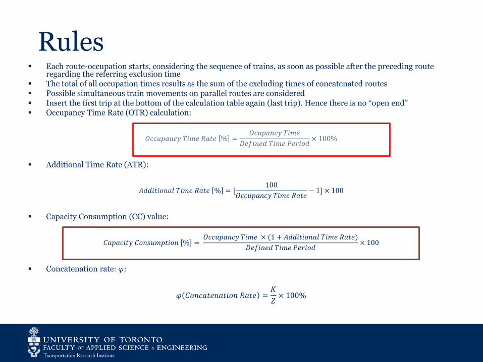
Rules Each route-occupation starts, considering the sequence of trains, as soon as possible after the preceding route
regarding the referring exclusion time The total of all occupation times results as the sum of the excluding times of concatenated routes Possible simultaneous train movements on parallel routes are considered Insert the first trip at the bottom of the calculation table again (last trip). Hence there is no “open end” Occupancy Time Rate (OTR) calculation:
𝑂𝑐𝑐𝑢𝑝𝑎𝑛𝑐𝑦 𝑇𝑖𝑚𝑒 𝑅𝑎𝑡𝑒 % =𝑂𝑐𝑢𝑝𝑎𝑛𝑐𝑦 𝑇𝑖𝑚𝑒
𝐷𝑒𝑓𝑖𝑛𝑒𝑑 𝑇𝑖𝑚𝑒 𝑃𝑒𝑟𝑖𝑜𝑑× 100%
Additional Time Rate (ATR):
𝐴𝑑𝑑𝑖𝑡𝑖𝑜𝑛𝑎𝑙 𝑇𝑖𝑚𝑒 𝑅𝑎𝑡𝑒 % = [100
𝑂𝑐𝑐𝑢𝑝𝑎𝑛𝑐𝑦 𝑇𝑖𝑚𝑒 𝑅𝑎𝑡𝑒− 1] × 100
Capacity Consumption (CC) value:
𝐶𝑎𝑝𝑎𝑐𝑖𝑡𝑦 𝐶𝑜𝑛𝑠𝑢𝑚𝑝𝑡𝑖𝑜𝑛 % =𝑂𝑐𝑐𝑢𝑝𝑎𝑛𝑐𝑦 𝑇𝑖𝑚𝑒 × (1 + 𝐴𝑑𝑑𝑖𝑡𝑖𝑜𝑛𝑎𝑙 𝑇𝑖𝑚𝑒 𝑅𝑎𝑡𝑒)
𝐷𝑒𝑓𝑖𝑛𝑒𝑑 𝑇𝑖𝑚𝑒 𝑃𝑒𝑟𝑖𝑜𝑑× 100
Concatenation rate: 𝜑:
𝜑 𝐶𝑜𝑛𝑐𝑎𝑡𝑒𝑛𝑎𝑡𝑖𝑜𝑛 𝑅𝑎𝑡𝑒 =𝐾
𝑍× 100%

Procedure to insert trains Main assumptions:
– All trains have through movements
– Uniform headway at every depot
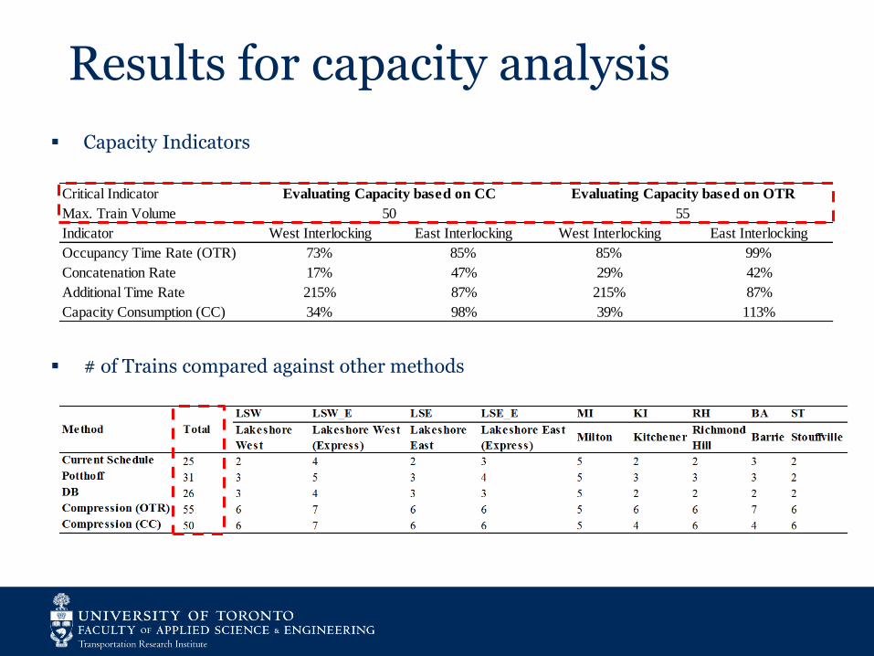
Results for capacity analysis
Capacity Indicators
# of Trains compared against other methods
Critical Indicator
Max. Train Volume
Indicator West Interlocking East Interlocking West Interlocking East Interlocking
Occupancy Time Rate (OTR) 73% 85% 85% 99%
Concatenation Rate 17% 47% 29% 42%
Additional Time Rate 215% 87% 215% 87%
Capacity Consumption (CC) 34% 98% 39% 113%
50 55
Evaluating Capacity based on CC Evaluating Capacity based on OTR

Effect of adding 1 trip
MethodCapacity
Indicator
West
Interlocking
East
Interlocking
Potthoff (B+R)/T 0.85 0.81
DB x 1.00 1.02
CompressionOTR 73% 85%
CC 34% 98%
West
Interlocking
East
Interlocking
0.90 0.96
0.97 0.8873% 85%34% 98%
Add 1 VIA trip
*Threshold for exceeding capacity:
(B+R)/T>=1 (Potthoff);
x <=1 (DB)

Discussion Potthoff and DB:
– timetable not required; – highly averaged results
Compression Method: – timetable required; – determined by the maximum occupancy of all train paths
within the same section; – possible to maximize the capacity with careful scheduling on
a timetable
Both require a matrix of occupancy time for conflicting paths:– only a pair of paths needs to be evaluated for conflicts– size of the matrix grows exponentially with the increase of
possible train paths
System stochasticity not considered

Railway Simulation
35

Railway Simulation
Simulation tools are recommended to analyze complex railway infrastructure
General procedure for simulation:
– Data collection
– Model construction
– Model calibration
– Model validation
OpenTrack was selected as the railway simulator
36

Model Construction
Main network (including maintenance yards) Expansion network including express stations
37

Model Input
Infrastructure layout
Speed limits
Train configurations (locomotive, rolling stock)
Schedules
Entry delay distributions
38

Entry Delay Distribution
Gotracker.ca
Weibull Lognormal Exponential Normal
Lognormal Exponential Lognormal Lognormal

Simulation Flow Chart

Performance Evaluation
Result evaluation:– Simulated On-time Performance (SOTP)
𝑆𝑂𝑇𝑃 =# 𝑜𝑓 𝑡𝑟𝑖𝑝𝑠 𝑎𝑟𝑟𝑖𝑣𝑒 𝑤𝑖𝑡ℎ𝑖𝑛 𝑎 𝑠𝑝𝑒𝑐𝑖𝑓𝑖𝑒𝑑 𝑟𝑎𝑛𝑔𝑒 𝑜𝑓 𝑠𝑐ℎ𝑒𝑑𝑢𝑙𝑒 𝑡𝑖𝑚𝑒
𝑡𝑜𝑡𝑎𝑙 # 𝑜𝑓 𝑡𝑟𝑖𝑝𝑠 𝑠𝑐ℎ𝑒𝑑𝑢𝑙𝑒𝑑× 100%
– Simulated Average Delay
GO Transit’s target On-time performance (OTP): 95%
OTP from data collection: 96.4%

Base model calibration and validation

Sensitivity Result
-5
0
5
10
15
20
25
30
20%
30%
40%
50%
60%
70%
80%
90%
100%
25 30 35 40 45 50 55 60 65 70
Avera
ged A
rriv
al D
ela
y at
Unio
n (
min
)
SO
TP
Total Train Volume
SOTP 95% Threshold Simulated Average Arrival Delay
Method Total # of Trains LSW LSW_E LSE LSE_E KI MI BA RH ST
OpenTrack 39 4 5 4 4 4 5 4 4 5
LSW: Lakeshore West Line
LSW_E: Lakeshore West Express
LSE: Lakeshore East Line
LSE_E: Lakeshore East Express
KI: Kitchener Line
MI: Milton Line
BA: Barrie Line
RH: Richmond Hill Line
ST: Stouffville Line

Discussion
OpenTrack offers a more realistic result by taking the stochasticity into consideration as it attempts to simulate the real-world operation
The result of between OpenTrack and Compression Method with OTR confirms that practical capacity is around 60% to 75% of the theoretical capacity from the previous research (Kraft, 1982)
LSW LSW_E LSE LSE_E MI KI RH BA ST
Lakeshore WestLakeshore West
(Express)Lakeshore East
Lakeshore East
(Express)Milton Kitchener
Richmond
HillBarrie Stouffville
Current Schedule 25 2 4 2 3 5 2 2 3 2
Potthoff 31 3 5 3 4 5 3 3 3 2
DB 26 3 4 3 3 5 2 2 2 2
Compression (OTR) 55 6 7 6 6 5 6 6 7 6
Compression (CC) 50 6 7 6 6 5 4 6 4 6
OpenTrack 39 4 5 4 4 5 4 4 4 5
TotalMethod
Method Total Trains LSW LSW_E LSE LSE_E KI MI BA RH ST
Compression (OTR) 55 6 7 6 6 5 6 6 7 6
OpenTrack 39 4 5 4 4 4 5 4 4 5
Ratio (%) 71% 67% 71% 67% 67% 80% 83% 67% 57% 83%

Problems
Dwell time was fixed at 5 minutes
Only focus on train movements on the railway
Pedestrian flow on the platform level could be complicated due to the platform layout and barriers
The interactive effect between train and pedestrian movements was not captured
45

Integrated Rail and Pedestrian Simulation- Nexus
46

Nexus
47
√

Dwell Time Components
Arrival Time Departure Time
Dwell Time
Doors
Open
Last
Passenger
Exits
Doors
Close
Segment
1
Segment
2
Segment
3Segment
4
Lost Time
Statistical Analysis
Lost TimeMassMotion
Internal Departure
Schedule
Assume a fixed value of 2 minutes
Passenger Flow Time
48

Alighting Behavior – Observation at Union
49

Problem Statement
The unique behavior would influence the density and crowding on the platform differently
The time that last passenger exit the train would affect the departure time of the train, especially for trains that become out of service after they arrive at Union, as trains cannot leave if passengers are still on board
Traditional Passenger flow time modeling cannot represent both effects properly (Total passenger flow time and density)
50

Method
Variables Extracted:
– Total passengers: 𝑇𝑃
– Turning point (%): 𝜌
– Passengers in segment a: 𝑇𝑃𝑎
– Flow rate in segment a: 𝑓𝑎
– Passengers in segment b: 𝑇𝑃𝑏
– Flow rate in segment b: 𝑓𝑏
Main Idea: represent the observed alighting curve with two linear lines with different flow rates
Each record of train door passenger count is studied, break point is selected based on visual inspection; linear regression is performed on the resulting segment a and segment b respectively; 𝑅2 values for the slopes of both lines are examined
𝑓𝑎
𝜌
𝑓𝑏

Data Analysis
Statistical analysis for 𝜌, 𝑓𝑎, 𝑓𝑏
• Correlation analysisTotal_Psg Total_Psg_seg_a Turning_Point Seg_a_Flow_Rate Psg_seg_b Seg_b_Flow_Rate
Total_Psg 1
Total_Psg_seg_a 0.911666804 1
Turning_Point -0.037696351 0.354965918 1
Seg_a_Flow_Rate 0.239571138 0.200437577 -0.068153854 1
Psg_seg_b 0.715672756 0.367111995 -0.678531836 0.197095319 1
Seg_b_Flow_Rate 0.578958678 0.347539801 -0.391475978 0.349225841 0.726731882 1

Model Proposed
Cumulative passenger volume
Time
𝑇𝑃
𝜌
𝑓𝑎
(Distribution)
(Input)
(Distribution)
𝑓𝑏 (Linear relationship) 𝑓𝑏 = 𝑇𝑃𝑏 ∙ 0.807 − 0.525= 𝑇𝑃 ∙ (1 − 𝜌) ∙ 0.807 − 0.525
𝑇
Alternative Observed Model
Avg. total time (sec) 104.1 107.1
Max. Total time (sec) 211.0 221.1

Pedestrian Simulation
MassMotion
54
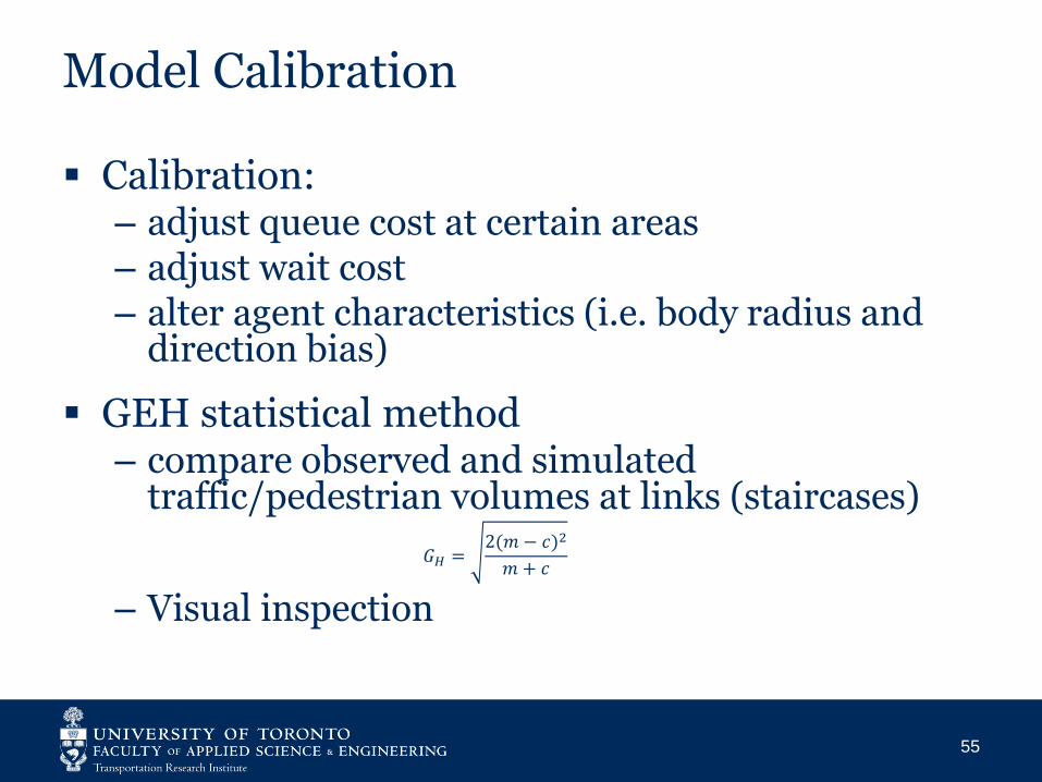
Model Calibration
Calibration:– adjust queue cost at certain areas– adjust wait cost– alter agent characteristics (i.e. body radius and
direction bias)
GEH statistical method– compare observed and simulated
traffic/pedestrian volumes at links (staircases)
𝐺𝐻 =2(𝑚 − 𝑐)2
𝑚+ 𝑐
– Visual inspection
55

Model Calibration and Validation
Validation
56

Nexus
57
√
√

Model Input
Individual simulation models (MassMotion, OpenTrack)
General Transit Feed Specification dataset (GTFS)
Complete list of agents with OD itinerary
58

Simulation Flow Chart
59

Model calibration and validation
60

Evaluating System Performance
Simulated On-time Performance (SOTP, %)
Simulate average arrival delay at Union (min)
Average dwell time (min)
Hourly inbound and outbound passenger volume (Person)
Average percentage of inbound and outbound passengers per second at LOS F (%)
Average duration at LOS F for each inbound and outbound passenger (Sec)
61
LOS Platforms (queueing) Stairways
Density (𝒑𝒆𝒓𝒔𝒐𝒏/𝒎𝟐) Space (𝒎𝟐/𝒑𝒆𝒓𝒔𝒐𝒏) Density (𝒑𝒆𝒓𝒔𝒐𝒏/𝒎𝟐) Space (𝒎𝟐/𝒑𝒆𝒓𝒔𝒐𝒏)
A x<=0.826 x>1.21 x<=0.541 x>=1.85
B 0.826<x<=1.075 1.21>x>=0.93 0.541<x<=0.719 1.85>x>=1.39
C 1.075<x<=1.538 0.93>x>=0.65 0.719<x<=1.076 1.39>x>=0.93
D 1.538<x<=3.571 0.65>x>=0.28 1.076<x<=1.539 0.93>x>=0.65
E 3.571<x<=5.263 0.28>x>=0.19 1.539<x<=2.702 0.65>x>=0.37
F 5.263<x 0.19>x 2.702<x 0.37>x

Scenario Tests
62

Scenario Tests
NEXUS
OpenTrack Model
MassMotion Model
Train Schedule
Population File
OpenTrack Sensitivity Test:
39 trains, 5 min dwell time
Person Capacity:
Peak Hour Factor (PHF))𝑃 = 𝑇 ∙ 𝑁𝑐 ∙ 𝑃𝑐 ∙ (𝑃𝐻𝐹
39 trains/h 12 Cars/Train 162 seats + 256 standees/car
63

Scenario Tests
Current schedule and
passenger volume
OpenTrack Sensitivity Test final schedule and
current level of train load
Train load increased by
adjusting the PHF to 0.49
PHF increased by 0.1 or
0.05 stepwise
Remove 2-minute buffer
time (segment 3 and 4)
Remove terminal passenger
alighting behavior
Assume a fixed value of 2 minutes
64
Base Model
Scenario 1
Scenario 2-5
Scenario 5A
Scenario 5B

Scenario Tests Results
65

Scenario Tests Results
9%
2 min
66

Scenario Tests Results
67

Scenario Tests Results
68
*total delay time (𝑛𝑢𝑚𝑏𝑒𝑟 𝑜𝑓 𝑝𝑎𝑠𝑠𝑒𝑛𝑔𝑒𝑟𝑠 × 𝑑𝑒𝑙𝑎𝑦)
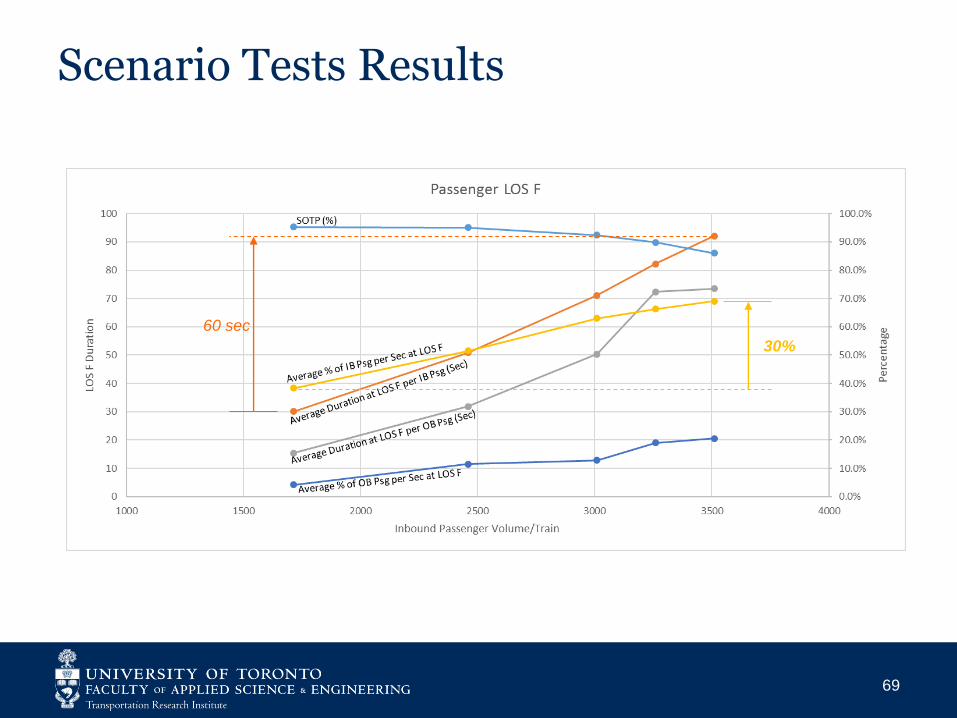
Scenario Tests Results
30%
60 sec
69

Scenario Tests Results
70
Inbound Outbound

Scenario Tests Results
Base Model
Scenario 5
71
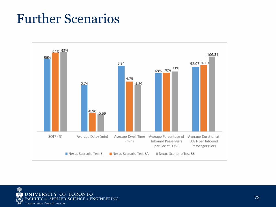
Further Scenarios
72

Conclusion
73

Conclusions
Analytical methods are not sufficient to capture the stochasticity of a complex area
Railway simulation fails to account for the impact of pedestrian movements
Both pedestrian movements and train movements have interactive effect on the total capacity of a complex station area
74

Contribution
Performed a comprehensive comparative analysis among various analytical and simulation methods on the capacity of a node area
Affirmed that practical capacity is around 60% to 75% of the theoretical capacity
Observed unique terminal passenger alighting behavior, proposed a simple initial model
Identified the benefit of using integrated simulation model
75

Future Work
Apply Nexus for new service concepts like RER
Study optimization methods
Consider the capacity of maintenance yards, turn-back movements at the Union Station
Further develop the alighting behavior model for the terminal station by considering other factors
Apply Nexus in other complex transit systems which are sensitive to delays
76

Acknowledgements
77

Thank you


![Mainline 1 [1]](https://static.fdocuments.us/doc/165x107/577d35831a28ab3a6b90a590/mainline-1-1.jpg)