CANONICAL QUANTIZATION OF SU(3) TOPOLOGICAL SOLITONS

VILNIUS UNIVERSITYINSTITUTE OF THEORETICAL PHYSICS AND ASTRONOMY

Darius Jurciukonis

CANONICAL QUANTIZATION OF SU(3)TOPOLOGICAL SOLITONS

Doctoral Dissertation

Physical Sciences, physics (02 P), mathematical and general theoretical physics,classical mechanics, quantum mechanics, relativity, gravitation, statistical physics,

thermodynamics (190 P)

Vilnius, 2008

The dissertation has been accomplished in 2003–2007 at the Vilnius University Institute of The-oretical Physics and Astronomy, Vilnius, Lithuania.

Scientific supervisor

Prof. Dr. Egidijus NORVAIŠAS, (Vilnius University Institute of Theoretical Physics andAstronomy, Physical Sciences, Physics – 02 P, mathematical and general theoretical phy-sics, classical mechanics, quantum mechanics, relativity, gravitation, statistical physics,thermodynamics – 190 P)

VILNIAUS UNIVERSITETOTEORINES FIZIKOS IR ASTRONOMIJOS INSTITUTAS

Darius Jurciukonis

SU(3) TOPOLOGINIU SOLITONUKANONINIS KVANTAVIMAS

Daktaro disertacija

Fiziniai mokslai, fizika (02 P), matematine ir bendroji teorine fizika, klasikinemechanika, kvantine mechanika, reliatyvizmas, gravitacija, statistine fizika,

termodinamika (190 P)

Vilnius, 2008

Disertacija rengta 2003–2007 metais Vilniaus universiteto teorines fizikos ir astronomijos insti-tute.

Mokslinis vadovas

prof. dr. Egidijus NORVAIŠAS (Teorines fizikos ir astronomijos institutas, fiziniai moks-lai, fizika – 02 P, matematine ir bendroji teorine fizika, klasikine mechanika, kvantinemechanika, reliatyvizmas, gravitacija, statistine fizika, termodinamika – 190 P)

Contents

Notations and conventions 7

List of publications 9

Preface 11

I. Introduction to Skyrme model 151. Historical remarks . . . . . . . . . . . . . . . . . . . . . . . . . . . . . . . . . 152. Nonlinear sigma model . . . . . . . . . . . . . . . . . . . . . . . . . . . . . . 173. The Skyrme model . . . . . . . . . . . . . . . . . . . . . . . . . . . . . . . . 204. The rational map approximation . . . . . . . . . . . . . . . . . . . . . . . . . 275. Generalization of the Skyrme model . . . . . . . . . . . . . . . . . . . . . . . 336. The Wess-Zumino term . . . . . . . . . . . . . . . . . . . . . . . . . . . . . . 357. Quantization of model . . . . . . . . . . . . . . . . . . . . . . . . . . . . . . 39

II. Canonical quantization of the SU(3) Skyrme model in a general represen-tation 431. Definitions for the unitary SU(3) soliton field . . . . . . . . . . . . . . . . . . 432. The Classical SU(3) Skyrme model . . . . . . . . . . . . . . . . . . . . . . . 463. Quantization of the skyrmion . . . . . . . . . . . . . . . . . . . . . . . . . . . 484. Structure of the Lagrangian and the Hamiltonian . . . . . . . . . . . . . . . . . 525. The symmetry breaking mass term . . . . . . . . . . . . . . . . . . . . . . . . 566. Summary . . . . . . . . . . . . . . . . . . . . . . . . . . . . . . . . . . . . . 57

III. Quantum SU(3) Skyrme model with the noncanonically embedded SO(3)soliton 591. Definitions for a soliton in the noncanonical SU(3) bases . . . . . . . . . . . . 592. Soliton quantization on the SU(3) manifold . . . . . . . . . . . . . . . . . . . 613. The structure of the Hamiltonian density and the symmetry breaking term . . . 644. Summary . . . . . . . . . . . . . . . . . . . . . . . . . . . . . . . . . . . . . 65

IV. Noncanonically embedded rational map soliton in the quantum SU(3) Skyrmemodel 671. Noncanonical embedding of the rational map soliton . . . . . . . . . . . . . . 672. Canonical quantization of the Soliton . . . . . . . . . . . . . . . . . . . . . . . 683. Summary . . . . . . . . . . . . . . . . . . . . . . . . . . . . . . . . . . . . . 73

Concluding statements 75

5

Appendix A. Definitions for the SU(2) soliton 77

Appendix B. Definitions for the SU(3) soliton 83

Appendix C. Definitions for the noncanonical SU(3) soliton 91

Appendix D. Calculations with computer algebra system 93

Santrauka 103

6

Notations and conventions

• Bold letters indicate multiple quantity structure, which may vary from case to case. Forexample, τ denotes a triple of Pauli matrices (τ1, τ2, τ3), r denotes the spatial vector ~r andU denotes the unitary field. Note that sometimes we do not follow this convention for thecoordinate q, momentum p and the variables α or κ in order to keep expressions morecompact.

• Calligraphic letters likeL,M,V ,H, etc. (with the exception of I andO) denote densities.

• The appearance of carets (R, L, J , etc.) indicate an operator or its component. Note thatwe do not follow this convention for the coordinate q and momentum p operators in orderto keep notations simpler. This is also true for operators which are functions of q only.

• The dot over a symbol (q, α, etc.) denotes the full time derivative.

• The metric tensor gµν is g00 = 1, g0,i = 0, gi,j = −δi,j for spatial indices i, j = 1, 2, 3.The derivative ∂µ ≡ ∂

∂xµhas components (∂/∂t,−∇). The sign of totally anti-symmetric

tensors (Levi-Cevita symbols) εijk and εµνσγ are fixed by ε123 = −ε123 = 1 and ε0123 =−ε0123 = 1, respectively.

• The isovector of Pauli isospin matrices τ in Cartesian coordinates have a form τ1 =(

0 11 0

),

τ2 =(

0 −ii 0

), τ3 =

(1 00 −1

).

• The symbol ∗ is a complex conjugation mark.

• The cross over some operators+

A denotes hermitically conjugate functions and is equiva-lent to notation A†.

• SU(2), SU(3), SO(3), SU(N), etc. denotes the symmetry groups.

• Greek letters α, β, γ . . . are the summation indices when used as upper indices. Theyalso represent Euler angles. The middle Greek letters λ, µ indicate representation of theSU(3) group, whereas θ, ϕ represent angles of the spherical coordinates. The Latin lettersa, b, c, d . . . are the summation indices usually. Minuscule letters j, l, m, n . . . indicateparameters of SU(2) group, whereas capital letters L, I, M,Z . . . represent parameters ofSU(3) or SO(3) groups. The index t denotes the time component.

• The symbol 1 denotes the unit matrix.

• The curly brackets{

,}

and the square brackets[,

]denote the anti-commutator and the

commutator, respectively.

7

8 Notations and conventions

• There is the assumed summation convention under the repeated (dummy) indices. The

symbol(λ,µ)∑

indicates summation over SU(2) group representations, which are included in(λ, µ) irreducible representation.

List of publications

1. D. Jurciukonis and E. Norvaišas, Quantum SU(3) Skyrme model with noncanonical em-bedded SO(3) soliton, J. Math. Phys., 48, 052101 (2007).

2. D. Jurciukonis and E. Norvaišas, Quantum SU(3) Skyrme model for arbitrary representa-tion, Bulg. J. Phys., 33 (s1b), 933 (2006).

3. D. Jurciukonis, E. Norvaišas and D.O. Riska, Canonical quantization of SU(3) Skyrmemodel in a general representation, J. Math. Phys., 46, 072103 (2005).

Contributions related to the dissertation at the following conferences:

• “V. International Symposium Quantum Theory and Symmetries (QTS-5)”, Valladolid,July 22–28, 2007.

• “37th Lithuanian National Conference of Physics”, Vilnius, June 11–13, 2007.

• “26th International Colloquium on Group Theoretical Methods in Physics”, New York,June 26–30, 2006.

• “IV. International Symposium Quantum Theory and Symmetries (QTS-4)”, Varna, August15–21, 2005.

• “6th Nordic Summer School in Nuclear Physics”, Copenhagen, August 8–19, 2005.


• “Physics in Warsaw 2004”, Summer School, Warsaw, September 20 – October 02, 2004.

• “Conference on Computational Physics 2004 (CCP-2004)”, Genoa, September 01–04,2004.


9

10 List of publications

PrefaceThe first suggestion that the ordinary proton and neutron might be viewed as topological solitonswas made by British physicist T.H.R. Skyrme in the sixties of last century. In his papers [1, 2]he has described nucleons as a liquid of pions by using a Lagrangian in which only two phe-nomenological constants were incorporated. The technology of the quantum field theory in thesixties was not sufficiently advanced to treat solitons and it took almost twenty years before theideas of Skyrme were revived by Witten [3] and Balachandran et al. [4]. The first demonstra-tion that the Skyrme model could fit the observed properties of the baryons to an accuracy ofabout 30% was made by Adkins et al. [5]. The model was subsequently refined and extendedin many ways. From phenomenological applications in elementary particle and nuclear physicsthe Skyrme model was applied to study the quantum Hall effect [6] and Bose-Einstein conden-sates [7] as well as in cosmology [8].

The equations of solitons are highly nonlinear and almost always are not solvable analytically,while the direct quantization of the solitonic solutions leads to rather complicated equations. Inour work we use the quantization in “zero modes” or “collective coordinate” approach [5, 9],which leads to a consistent quantum description. Using the canonical quantization we considerthe Skyrme Lagrangian quantum mechanically ab initio. In this case the generalized coordinatesand velocities do not commute. The canonical quantization leads to quantum corrections, whichstabilize the soliton solutions. To obtain Euler-Lagrange equations, that are consistent with thecanonical equation of motion of the Hamiltonian, the general method of quantization on a curvedspace developed by Sugano et al. [10] is employed.

The Skyrme model is usually formulated in the fundamental representation of SU(2) group,where the field is a unitary 2 × 2 matrix. The model can also be generalized to unitary fields,that belong to general representations of the SU(2) [11–13], along with a demonstration that thequantum corrections are representation dependent.

The quantum SU(3) Skyrme model was generalized to arbitrary representation as well [14].The algebraic structure of the SU(3) group is more plentiful, consequently it is possible to usevarious classical solutions for the quantization. The choice of the noncanonically embeddedsoliton is explored in Ref. [15]. The formalism of the noncanonical embedded soliton can beexpanded for the description of multisolitonic states by using rational map approximation. Thesequestions are considered in this dissertation.

The main goals of the research work

1. To investigate representation dependence of the canonically quantized SU(3) Skyrme model.

2. To explore the SU(3) Skyrme model with a noncanonically embedded SU(3) ⊃ SO(3)soliton.

3. To investigate the SU(3) Skyrme model with the noncanonically embedded SU(3) ⊃SO(3) soliton by using the rational map approximation with the baryon number B ≥ 2.

11

12 Preface

Scientific novelty

This work exposes new possibilities of the extended basic SU(3) Skyrme model to general ir-reducible representations (λ, µ). The strict canonical quantization of the model yields fromrepresentation depended Lagrangian density, which can be treated as different solitons, conside-ring different representations. The classical limit of these quantum Lagrangian densities is theusual SU(3) Skyrme Lagrangian density. A new, nontrivial dependence in Wess-Zumino and thesymmetry breaking terms on the representation was observed.

The new ansatz for the Skyrme model is introduced. It is defined in the noncanonical SU(3) ⊃SO(3) bases. Quantization of the soliton leads to new expressions of the soliton momenta ofinertia and quantum mass corrections. The rational map approximation for the Skyrme modelwith noncanonically embedded ansatz is applied. This leads to five different quantum momentsof inertia and new quantum mass corrections. The explored ansatz can be used in nuclear physicsto describe a light nucleus.

Generalizations considered in the work are significant and can be extended to other modelsand theories.

Thesis statements

1. Different Lagrangian and Hamiltonian operators of the quantum SU(3) Skyrme modelfor different representations (λ, µ) were found. The explicit dependence on the repre-sentation of the Wess-Zumino term, the symmetry breaking term and the quantum masscorrections were derived in the framework of the canonical quantization. The dependenceon the irreducible representation (λ, µ) of the SU(3) group can be treated as a new discretephenomenological parameter of the model.

2. A new version of the Skyrme model is obtained introducing the new ansatz, which is de-fined in the noncanonical SU(3) ⊃ SO(3) base. This is confirmed by the new expressionsof the soliton momenta of inertia and the quantum mass corrections.

3. The topological solitons carrying baryon number B ≥ 2 can be described using the ra-tional map approximation ansatz, which is a noncanonically embedded SU(3) ⊃ SO(3)soliton. The canonical quantization leads to five different quantum moments of inertia andnew quantum mass corrections.

Approbation of the results

Main results of the research described in this dissertation have been published in 3 scientificpapers and a few talks in the international conferences. A detailed list of publications is given inprevious section.

Personal contribution of the author

The author of the thesis performed many analytical derivations of the equations (shown in chap-ters II – IV and the appendices) by using “pencil” and majority calculations by using computeralgebra system MATHEMATICA.

Preface 13

Manuscript organization

The manuscript is organized into four chapters and four appendices, containing some auxiliaryexpressions connected with the analyzed problems in the dissertation. The chapters have shortintroductions in the beginning, research of the problem and summaries at the end. It is useful todescribe the purpose of each chapter. Chapter I contains the mathematical formulation and thephysical motivation of the Skyrme model at the background level. This chapter contains no newresults. Chapter II describes the representation dependence of the canonically quantized SU(3)Skyrmion. This chapter includes results of Ref. [14]. The formulation of the SU(3) Skyrmemodel with the noncanonically embedded SU(3) ⊃ SO(3) soliton is presented in Chapter IIIfollowing Ref. [15]. The rational map approximation for the Skyrme model with the noncano-nically embedded ansatz is explored in Chapter IV.

Acknowledgements

First of all I would like to thank my supervisor and collaborator Egidijus NORVAIŠAS, forhis patient, friendly and unfailing guidance and support over the past five years. Many thanksto Arturas ACUS for careful reading of the manuscript and help with MATHEMATICA. I amgrateful to Sigitas ALIŠAUSKAS, Andrius JUODAGALVIS and Vidas REGELSKIS from theDepartment of the Theory of Nucleus for support and friendship. Also many thanks to JuliusRUSECKAS for assistance and interesting discussions. Finally I would like to thank manyothers at Institute of Theoretical Physics and Astronomy of Vilnius University, and especially toAlicija KUPLIAUSKIENE and Gintaras MERKELIS for consultations and support connectedto PhD studies.

14 Preface

I. Introduction to Skyrme model

1. Historical remarksWhile deep inelastic electron-scattering experiments at high energy show the baryons to consistof quarks, no such simplicity is revealed by the low energy observables of the baryons. In fact thelow energy structure of the baryons appears to represent the full complexity of the “vacuum” ofquantum chromodynamics (QCD), a description of which is entirely outside of the realm of theextant perturbative methods of QCD. On the other hand, description of the baryon structure andinteractions on the basis of effective chiral meson models has been developed. The challengehas therefore been to find a sound basis in QCD for this effective mesonic description. Themain task was to develop non-perturbative approaches to QCD, which could replace the basicdynamical quark and gluon degrees of freedom by observable meson fields.

When the original fermion theory (QCD) is replaced by an effective boson theory, the fermions(baryons) have to be described as soliton solutions, which are topologically stable, with a con-served integer quantum number that is to be interpreted as the baryon number [3, 16]. The onlyfundamental symmetry that survives the procedure of replacing the fundamental fields by theeffective meson fields is the chiral symmetry of QCD. Various models were created based onthe nonlinear chiral meson field theory. Their topological soliton solutions can be quantised asfermions. The simplest of these models is the Skyrme model proposed by T.H.R. Skyrme in thesixties of last century [1].

The Skyrme model is the simplest extension of the nonlinear σ-model [17] that has stablesoliton solutions with an integral baryon number. It represents a theory for an interacting pionfield, in which the interactions are introduced through a chirally symmetric constraint involvingan auxiliary scalar meson field, σ. Although a bosonic representation of QCD should involveinfinitely many meson fields, one expects only the lightest mesons to be of quantitative signi-ficance for the low energy properties of the baryons (and nuclei in general). Hence a naturalstarting point for the description of the low energy behaviour of the baryons is to use the Skyrmemodel and its immediate generalizations, which incorporate vector meson fields [18–20]. Thesmall number of parameters of the Lagrangian model are in principle obtainable from QCD, butin practice they have to be chosen to fit some of the observables.

The technology of the quantum field theory in the sixties was not sufficiently advanced to treatsolitons, so it took almost twenty years before the ideas of Skyrme were revived by Witten [3]and Balachandran et al. [4]. The first demonstration that the Skyrme model, in spite of itssimplicity with only two parameters in the Lagrangian density, can provide a description ofthe static properties of the non-strange baryons was made by Adkins et al. [5]. The predictedobservables were found to differ from their empirical values by less than 30%. The modelwas subsequently refined in many ways. The correct asymptotic behaviour of the soliton fieldwas achieved by an introduction of a chiral symmetry breaking mass term [21]. Alternativeand augmented forms for the basic Lagrangian density have been studied [22, 23]. In addition,different generalizations of the Skyrme model that contain explicit vector meson fields have

15

16 I. Introduction to Skyrme model

been developed [18–20] and applied to the analysis of baryon structure [24]. In general therefinements of the topological soliton model have led to improved predictions of the low energybaryon observables, although certain systematic discrepancies remain, among them the constantunderprediction of the axial-vector coupling constant.

One way of looking at these systematic quantitative shortcomings of the topological solitonmodel is to view the model as the zero-size limit of the chiral bag with an external mesonfield [25]. By replacing the central region by an explicit quark bag, which is stabilised by theexternal soliton field, the quark colour number Nc appears in the formulae as a parameter. Thenit becomes obvious that the pure soliton model can be viewed as a large-Nc limit of the chiral bagmodel. In particular, it becomes clear that a factor 5/3 in the axial coupling constant is lost in thepure soliton limit, which is probably the main reason for the underprediction of this observablein the soliton model [26].

The study of the static baryon observables in the two-phase chiral bag model has also provento be very useful because it has led to the conclusion that these observables are insensitive to thebag size [27]. This is sometimes referred to as the “Cheshire cat” principle, the essential contentof which is that the low energy properties of the baryons can be described in equivalent ways interms of quarks and gluons or meson fields, making the choice of language one of conveniencerather than one of essence. In practice, the consistent treatment of the complete chiral bag modelis rather subtle. Once the baryon number is divided, with a fraction carried by the soliton field,the sea quark contributions must be included as the valence quarks alone always give an integerbaryon number [28]. A further complication is due to the need to rotate the soliton field and thequark bag in a consistent way for the projection onto states of good spin and isospin [27].

These and other difficulties associated with the use of the complete chiral bag model makesit natural to lean heavily on the Cheshire cat principle and to exploit all reasonable possibilitiesof refining the pure topological soliton model before resorting to the two-phase model. This ap-proach has in fact been fairly successful. Using versions of the model that contain explicit vectormeson fields one obtains a fairly good description not only of the static baryon observables, butof the baryon form factors as well [24].

The application of the topological soliton model to the interacting two-nucleon system wasalso proven to be extremely fruitful. While the need for mathematical approximations has ham-pered the study of the interaction operators at short distances, sufficiently accurate approxima-tion methods have permitted the study of their long-range behaviours. Thus, many importantfeatures of the nucleon-nucleon interaction are predicted by the simplest original version of themodel. Among these are the one-pion-exchange interaction [2], the short-range repulsion [26]and the isospin-dependent spin-orbit interaction [29].

The Skyrme model can also be used to study elementary particle dynamics, e.g. pion-nucleonscattering. To describe pion-nucleon scattering in the Skyrme model, an external pion field has tobe coupled to the soliton field. This can be done in several formally different ways [30–32]. Thesimplest method is that of Schnitzer [30,33], which leads to the usual Weinberg Lagrangian [34]for the pion-nucleon system in the quadratic approximation. Studies of pion-nucleon scatteringamplitudes using the Skyrme model have led to interesting relations between different partialwave amplitudes, which appear to be satisfied empirically [31, 32].

The generalization of the Skyrme model from the SU(2) to the SU(3) flavor symmetry for a de-scription of the strange hyperons was proven to be very interesting. The straightforward methodof incorporation of strange hyperons to the model corresponds in the quark-model language totreating the strange (s) quark on the same footing as the non-strange (u, d) quarks. This leads to a

2. Nonlinear sigma model 17

description of the hyperons in terms of the SU(3) collective coordinates, in which both the kaonsand the pions are massless in the first approximation. Although first attempts along these linesseemed to be successful [35, 36] but it latter appeared that the direct extension of the model,in which the isospin group is enlarged and the strangeness is treated in the same way as theisospin, does not give a quantitatively acceptable description of the hyperon spectrum [37, 38].An alternative approach is the bound-state model due to Callan and Klebanov [39], in whichthe strange hyperons are described as bound states of the SU(2) solitons (skyrmions) and thestrangeness-carrying kaons. This approach leads to an acceptable description of the spectrumof the stable hyperons [40, 41], and to the values of their magnetic moments that differ from theempirical ones by less than 20% [42, 43]. This model for the hyperons has intrinsic interest aswell, as it corresponds to an exotic atom where bosonic kaons with a half-integer charge andspin are in the bound-state orbits.

A new feature in all SU(3) extensions of the Skyrme model is the fact that the Wess–Zuminointeraction [3,44,45] contributes to the energy. As this interaction is linear in its time derivative,it can distinguish positive and negative frequencies in such a way that for a positive baryonnumber only the states of the negative strangeness are bound. In the SU(2) Skyrme model, theWess–Zumino interaction is (for the same reason) essential in that it, causes the state vector ofthe system to change its sign under a spatial rotation by 360◦ if the number of colours is odd [3].However there is no contribution to the energy in this case.

The extension of the model to the SU(N) group [46] represents the common structure of theSkyrme Lagrangian. Most of the studies involving the Skyrme model have concentrated on theSU(2) version of the model and its embeddings into the SU(N). However, considering SU(N)for N ≥ 3, one has to bear in mind that the Skyrme model is not unique. In fact, there are twopossible versions of the fourth-order Skyrme term. Another way is to be studied model based onthe alternative form of the fourth-order Skyrme term [47].

Very little attention has been paid to field configurations describing many skyrmions in theSU(N) models which were not embeddings of the SU(2) skyrmions. Although some work hasbeen done earlier [4, 48] the real progress has only been made since Houghton, Manton andSutcliffe had produced their harmonic map antsatz [49]. This ansatz, when generalized to theSU(N) models [50], has lead to the construction of whole families of solutions of the SU(N)Skyrme models having spherically symmetric energy densities [51]. Moreover, it also presentsfield configurations, which although are not solutions of the equations, are close to them – thusproviding us with good approximates to other solutions [50].

2. Nonlinear sigma model

The low energy properties of QCD mostly relevant to nuclear physics are dominated by the lightquarks u, d and s. The masses of the u- and d-quarks (∼ 10 MeV) are small compared to the QCDcutoff (∼ 200 MeV). If these masses are neglected, the QCD Lagrangian becomes invariant un-der SU(2)L ⊗ SU(2)R chiral transformations. The absence of the parity doublets in the physicalspectrum suggests that this symmetry is spontaneously broken to the SU(2)V vector symmetryvia the Nambu-Goldstone mechanism, with the appearance of 3 massless pseudoscalar excita-tions: π0, π±. In other words the QCD ground state carries an axial charge. As a result pionscan decay into the vacuum.

In the absence of the quantitative understanding of non-perturbative QCD an alternative is


provided at low energy by effective chiral descriptions of which the nonlinear σ-model consti-tutes the starting point. While QCD is undoubtedly a fundamental theory of hadrons, the chiralfield models are specifically designed approximations to hadron dynamics, suited for low energytreatment.

The essence of chiral symmetry and the relative success of current algebra lies in the fact thatthe vacuum state in QCD spontaneously breaks the chiral symmetry. If we denote a pion stateof momentum p by |πi(p)〉 and the axial-vector current by Ai

µ(x) then

〈0|Aiµ(x)

∣∣πj(p)⟩

= ifπpµeipxδij, (I.2.1)

where fπ = 130.7 MeV is the observed pion decay constant and i =√−1.

Due to the non-perturbative character of QCD in the long wavelength approximation verylittle is known about the pion decay constant fπ and the nucleon axial form factor gA from firstprinciples. There is no doubt that ultimately, lattice gauge calculations will provide a quantitativeunderstanding of these low energy parameters. Meanwhile, the large Nc limit as advocated by’t Hooft [52] and Witten [53] is suggestive of an effective mesonic description involving thedominant chiral degrees of freedom π0, π±, as a substitute to QCD at low energy. AlthoughNc = 3 and not infinity, one hopes that this approach will provide the relevant starting lines fordiscussing low energy phenomenology. In this spirit the nonlinear σ-model provides a pertinentscript for chiral symmetry breaking, consistent with soft-pion threshold theorems. If we denotethe scalar meson field by σ(x) and the pseudoscalar pion field by π, then the resulting dynamics,described by

Lσ =1

2(∂µσ)2 +

1

2(∂µπ)2 , σ2 + π2 = f 2

π , (I.2.2)

is manifestly chiral invariant since(

σπ

)corresponds to the (1, 0) representation of

SU(2)L ⊗ SU(2)R ∼ SO(4).In the trivial vacuum the nonlinear condition (I.2.2) translates into 〈0|σ |0〉 = fπ, which is the

expected limit if one uses the linear σ-model with an infinitely heavy scalar particle (mσ →∞).To account for the small but non vanishing mass of the pion field in nature, one adds an explicitchiral breaking term in the form LCb = −cσ. In the trivial vacuum, the pion can be understoodas fluctuations of the σ-field along the valley of the tilted Mexican hat,

LCb = −cσ = −c√

f 2π − π2 = −cfπ +

c

2

π2

fπ

+O(

1

f 3π

). (I.2.3)

Already at this stage we can see that the nonlinear σ model satisfies the basic low energyrequirements solely on the basis of chiral symmetry. It embodies an underlying topologicalstructure that yields non-perturbative field configurations reminiscent of classical baryons.

To grasp the geometrical intricacies of the nonlinear σ-model, it is instructive to recast it inthe Sugawara form [1, 2]. For that, lets define the unitary 2× 2 quaternion field U(x)

U(x) =1

fπ

(σ + iτ · π) , (I.2.4)

that transforms as the(

12, 1

2

)representation of SU(2)L × SU(2)R,

U(x) → exp(iQL)U exp(−iQR); QL ∈ SU(2)L; QR ∈ SU(2)R. (I.2.5)

2. Nonlinear sigma model 19

In the quark picture the analogue of U ij is the complex 2 × 2 matrix q−i[(1 − γ5)/2]qj corres-ponding to pseudoscalar mesons [54]. U(x) ∈ SU(2) whose group manifold is isomorphic toS3. The left and right currents on S3 are defined to be

Rµ = ∂µUU † → exp(iQL)Rµ exp(iQL), (I.2.6a)

Lµ = U †∂µU → exp(iQR)Lµ exp(−iQR), (I.2.6b)

which show that Rµ (Lµ) is invariant under right (left) chiral transformations. Since det U = 1,it follows that

∂µ det U = ∂µ exp Tr(ln U

)= Tr

(Lµ

)= Tr

(Rµ

)= 0. (I.2.7)

It is instructive to note that for a weak pion field Lµ and Rµ reduce to

Lµ ∼ −Rµ ∼ i

fπ

τ · ∂µπ. (I.2.8)

At any fixed time, the 2 × 2 field U(x) defines a map from the three dimensional space R3

onto the group manifold S3, with the natural boundary condition that U(x) goes to the trivialvacuum 〈0|σ |0〉 = fπ at asymptotically large distances. This ensures that the energy of thecorresponding field configuration is finite and

U(|x| → ∞) = 1 (I.2.9)

implies that R3 is compactified to S3 as all points at infinity in R3 are mapped into one fixedpoint in S3. The set of static maps subject to (I.2.9),

U(x) : S3 → S3, (I.2.10)

is known to be non trivial. In other words, at a given time, it is possible to split the set of allmaps into homotopically distinct classes not continuously deformable into each other. Theseclasses are called the homotopy or Chern-Pontryagin classes. In this case, they constitute thethird homotopy group π3(S3) ∼ Z, where Z is the additive group of integers. It is these integersthat are referred to as winding numbers of the mapping U(x). Since a continuous evolution intime can be understood as a homotopy transformation, the corresponding winding numbers areconserved by definition independently of the details of the underlying dynamics.

In order to construct an explicit form of the topological charge B0 in the nonlinear σ-model:

B0 : π3(S3) → Z, (I.2.11)

it is convenient to use the vector representation (1, 0) of SU(2)L ⊗ SU(2)R,

φ0 =σ

fπ

, φi =πi

fπ

. (I.2.12)

An elementary surface element in the group manifold is characterized by

d3Σ = εijklφi∂1φj∂2φ

k∂3φldx1dx2dx3, (I.2.13)

where (x1, x2, x3) are the corresponding coordinates onR3 obtained by stereographic projectionfrom S3. Equation (I.2.13) is just the Jacobian associated to the affine transformation S3 → S3.Hence, the normalized topological density reads

B0 =1

3!A3

εijklεναβφi∂νφj∂αφk∂βφl, (I.2.14)


where A3 = 2π2 is the surface of S3 in R4 . To rewrite the equation (I.2.14) in terms of (I.2.6),notice that for a weak pion field, i.e. φ0 ∼ 1/fπ and φi ∼ πi/fπ. We have

B0 =(−i)3

24π2εναβ Tr

(∂ν

(iτ · π

fπ

)∂α

(iτ · π

fπ

)∂β

(iτ · π

fπ

))+O

(1

f 4π

)

=− i

24π2ε0ναβ Tr

(RνRαRβ

). (I.2.15)

This equation follows from the chiral invariance. Notice that B does not vanish if and only if the3 pion degrees of freedom, π0, π±, are excited. It is rather obvious from the above constructionthat

B =

∫

R3

B0dx = winding number. (I.2.16)

The covariant current associated to the topological charge (I.2.15) is given by

Bµ = − i

24π2εµνβγ Tr

(RνRβRγ

), (I.2.17)

and is conserved almost everywhere in R3 independently of the equations of motion,i.e. ∂µBµ = 0.

The topological charge (I.2.15) bears some similarities with the monopole and instantoncharges. It follows from the underlying Riemannian structure of the group manifold and isconserved regardless of the equations of motion. Its form is obtained by an explicit construc-tion of the isomorphism: π3(S3) ∼ Z . The topological charge has no dual charge, and can belocalized arbitrarily in space since (I.2.15) is not a total divergence.

3. The Skyrme model

So far the nonlinear σ-model has provided a rather economical framework for discussing lowenergy phenomenology. Its finite energy configuration space exhibits a nontrivial topologicalstructure due to the underlying Riemannian geometry of the coset space. As a consequence, thereexist static and finite field configurations other than the trivial vacuum, that are characterized byconserved topological charges. Unfortunately, these configurations are not energetically stablein 3 dimensional space according to Derrick’s theorem [55, 56]. Indeed, if U(x) is a static fieldconfiguration solution to the Euler-Lagrange equations associated to

Lσ = −f 2π

4Tr

(RµR

µ), (I.3.18)

which is the Sugawara’s form of (I.2.2), then

E =

∫dDx

f 2π

4Tr

(∂iU †∂iU

). (I.3.19)

A simple rescaling of U(x) in space, i.e. U(x) → U(λx), yields

Eλ = λ2−DE. (I.3.20)

3. The Skyrme model 21

Equation (I.3.20) clearly shows that for D = 3, the energetically favorable configurations havezero energy. In other words the finite energy solutions of the nonlinear σ-model are unstableagainst scale transformations.

To avoid this collapse, Skyrme added to (I.3.18) a quartic term in the currents Rµ (the Skyrmeterm),

LSk = −f 2π

4Tr

(RµR

µ)

+1

32e2Tr

([Rµ, Rν ][R

µ, Rν ]). (I.3.21)

Here e is a dimensionless parameter that characterizes the size of the finite energy configurations.The values of parameters fπ and e are fixed by comparison with the experimental data.

The Euler-Lagrange equation which follows from (I.3.21) is the Skyrme field equation

∂µ

(Rµ +

1

8f 2πe2

[Rν , [Rν , R

µ]])

= 0, (I.3.22)

which is a nonlinear wave equation for U(x). The Bogomolny construction to simplify (I.3.22)via saturation mechanism to obtain analytical solutions (a well known procedure for instantons)cannot be used in this case. A numerical treatment of (I.3.22) is required.

Since the Skyrme term scales like r−4 in the three dimensional space it will prevent the Skyrmesolitons from collapsing to zero size. Indeed, a rescaling in space of any finite energy solutionof (I.3.21) translates to a rescaling in the ground state energy in the form

Eλ = λ2−DE(2) + λ4−DE(4). (I.3.23)

It is straightforward to show that Eλ exhibits a true minimum for D ≥ 3, i.e.,

dEλ

dλ= 0 → E(2)

E(4)

= −D − 4

D − 2, (I.3.24a)

d2Eλ

dλ2> 0 → 2(D − 2)E(2) > 0 . (I.3.24b)

In particular for D = 3 the equation (I.3.24a) shows that E(2) = E(4), as expected from the virialtheorem. Due to the underlying geometry, the energy is bounded from below by the topologicalcharge. Indeed, for a static configuration

E =

∫d3x

(−f 2

π

4Tr

(R2

i

)− 1

32e2Tr

([Ri, Rj]

2))

. (I.3.25)

A lower bound to (I.3.25) can be obtained using the following inequality,∫

d3x Tr

(f 2

π

2R2

i +1

8e2εijk[Rj, Rk]

)2

≤ 0. (I.3.26)

where this facts are used that the Ri’s are anti-Hermitian matrices and that for any anti-Hermitianmatrix G, Tr

(G2

) ≤ 0. In terms of the topological charge B, this becomes

E ≥ 6π2fπ

e|B| . (I.3.27)

Equation (I.3.27) is sometimes referred to as the Bogomolny bound [57]. Since there are noself dual chiral fields, the energy is strictly larger than the estimate (I.3.27). For skyrmions


the Bogomolny bound cannot be saturated. Equation (I.3.27) illustrates in a striking way themechanism by which geometry induces local stability at the classical level.

The Skyrme term can be understood as a higher-order correction to the nonlinear σ-modelwhen cast in the general framework of an effective chiral description as advocated by Weinberg[58]. While the quadratic term (I.3.18) in the nonlinear σ-model is only one chirally invariantterm of the second order, the fourth order term is not unique to order chirally invariance. Indeed,under the general assumptions of locality, the Lorentz invariance, the chiral symmetry, the parityand the G-parity there are 3 independent terms to order chirally invariance, i.e.

L(4) = a Tr(RµR

µRνRν)

+ b Tr(RµRνR

µRν)

+ c Tr(∂µRν∂

µRν), (I.3.28)

where a, b, c are some constants. Other combinations can be eliminated by the Maurer-Cartanequation for the right current on S3

∂µRν − ∂νRµ + [Rµ, Rν ] = 0, (I.3.29)

which follows trivially from the definitions (I.2.6). To this order, the combination:

L(4) = Tr(RµR

µRνRν)− Tr

(RµRνR

µRν)

= −1

2Tr

([Rµ, Rν ][R

µ, Rν ]), (I.3.30)

is the unique term with four derivatives that leads to a Hamiltonian having the second orderin time derivatives. (I.3.30) is exactly the term suggested by T. H. R. Skyrme [59]. This isimportant because there are problems with the stability of the classical solution, once higherorder terms in the time derivatives are included.

After the baryon number and energy, the most significant characteristic of the static solutionof the Skyrme equation is its asymptotic field, which satisfies the linearized form of the equation.To the leading order, each of the three components of the pion field π obey Laplace’s equation,and σ can be taken to be unity. More precisely, π has a multipole expansion, in which each termis an inverse power of r = |x|, say r−(l+1), times a triplet of angular functions. The leadingterm, with the smallest l, obeys Laplace’s equation, whereas subleading terms may not, becauseof the nonlinear aspect of the Skyrme equation. For the leading term, therefore, the angularfunctions are a triplet of the linear combinations of the spherical harmonics Yl,m(θ, ϕ), with mtaking integer values in the range−l ≤ m ≤ l. These spherical harmonics can also be expressedin the Cartesian coordinates, which often gives more convenient and elegant formulae for theasymptotic fields.

One of the few precise results concerning the Skyrme equation (I.3.22) is that this multipoleexpansion can not lead with a monopole term, having l = 0. The leading term is a dipole orhigher multipole [60].

Recently, it has been rigorously proven [61] that for any non-vacuum soliton of the Skyrmeequation, the multipole expansion is non-trivial. In other words, the pion field does not vanishto all orders in l, and the leading term is a multipole satisfying the Laplace equation.

The skyrmionIn his pioneering work Skyrme [1] believed that the field configurations of the winding numberone (B = 1) were fermions. He conjectured that the topological current (I.2.17) should beidentified with the baryon current, suggesting that skyrmions were classical baryons.


The classical Skyrme model is formulated in the arbitrary irreducible SU(2) representationj [11]. The Euler angles α(x, t) become the functions of the space-time point (x, t) and formthe dynamical variables of the theory. Model is formulated in terms of a unitary field

U(x, t) = Dj(α(x, t)

), (I.3.31)

where symbol Dj denotes the SU(2) Wigner matrices.By using definitions from Appendix A allow us to express the Lagrangian density (I.3.21) in

terms of the Euler angles

LSk =1

3j(j + 1)(2j + 1)

(f 2

π

4

(∂µα

i∂µαi + 2 cos α2 ∂µα1 ∂µα3

)

− 1

16e2

(∂µα

2∂µα2(∂να1∂να1 + ∂να

3∂να3)− (∂µα1∂µα2)2

− (∂µα2∂µα3)2 + sin2α2(∂µα

1∂µα1 ∂να3∂να3 − (∂µα

1∂µα3)2)

+ 2 cos α2(∂µα2∂µα2 ∂να

1∂να3 − ∂µα1∂µα2∂να

2∂να3)))

. (I.3.32)

The only dependence on the dimension of the representation is in the overall factorj(j + 1)(2j + 1) as it could be expected from the inner product of two SU(2) generators. Thisimplies that the equation of motion for the dynamical variable α is independent of the dimensionof the representation.

In terms of the Euler angles α the baryon current density takes the form

Bµ =1

24Nπ2εµνβγ Tr

(RνRβRγ

)

=− 1

24 · 6Nπ2j(j + 1)(2j + 1) sin α2 εµνβγ εikl ∂να

i∂βαk∂γαl. (I.3.33)

The normalization factor N depends on the dimension of the representation and has the value 1in the fundamental (j = 1/2) representation. As the dimensionality of the representation appearsin this expression in the same overall factor as in the Lagrangian density (I.3.32) it follows thatall calculated dynamical observables will be independent of the dimension of the representationat the classical level.

The equation of motion (I.3.22), which follows from the variation of the Lagrangian (I.3.21),are highly nonlinear and so far can only be handled under the assumption of maximal symmetryas suggested by Skyrme’s static hedgehog ansatz [2]

U(x) = exp (iτ · rF (r))

= cos F (r) + iτ · r sin F (r). (I.3.34)

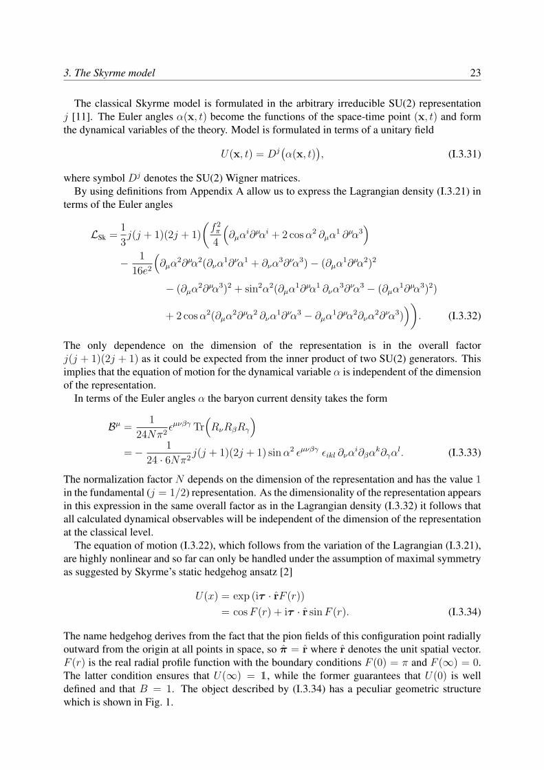
The name hedgehog derives from the fact that the pion fields of this configuration point radiallyoutward from the origin at all points in space, so π = r where r denotes the unit spatial vector.F (r) is the real radial profile function with the boundary conditions F (0) = π and F (∞) = 0.The latter condition ensures that U(∞) = 1, while the former guarantees that U(0) is welldefined and that B = 1. The object described by (I.3.34) has a peculiar geometric structurewhich is shown in Fig. 1.


Figure 1: The hedgehog configuration [62].

The Equation (I.3.34) follows from the fact that in a given topological sector, the maximalcompact symmetry group of the configuration space is

diag (SU(2)L ⊗ SU(2)R) ∼ diag (SO(2)I ⊗ SO(3)J) , (I.3.35)

where SO(3)J and SO(3)I refer to the orthogonal group of rotations in space and isospace re-spectively. In the ansatz (I.3.34 ), the isospin (I) and the angular momentum (J) are correlatedin a way that neither of them is good quantum number, but their sum is

K = J + I ≡ (L + S) + I. (I.3.36)

U(x) is left invariant under rotations in K-space, i.e.

[K, U(x)

]= i sin F

([(r× ∇

i

), τ · r

]+

[τ/2, τ · r]

)

= i sin F (−i (τ × r)− i (r× τ )) ≡ 0, (I.3.37)

suggesting that hedgehog skyrmions are scalar in K-space (K = 0). Since parity is definedthrough

πopU(x, t)π−1op = U †(−x, t), (I.3.38)

one concludes that the ansatz (I.3.34) is parity invariant. Here πop is the parity operator. Con-sequently, hedgehog skyrmions carry Kπ = 0+ and can be viewed as a mixture of states withI = J and the positive parity.

The substitution of the hedgehog ansatz (I.3.34) into the Lagrangian density (I.3.21) leads tothe following form:

LSk = −4

3j(j + 1)(2j + 1)

(f 2

π

4

(F ′2 +

2

r2sin2F

)

+1

4e2

sin2F

r2

(2F ′2 +

sin2F

r2

)). (I.3.39)


0 1 2 3 4 5r�

1

2

Π

F

Figure 2: A classical solution of the profile function F (r) forthe B = 1 skyrmion.

For the case of j = 1/2 this reduces to the result of [5]. The corresponding mass density isobtained by reverting the sign of LSk, as the hedgehog ansatz is a static solution.

The requirement that the soliton mass is stationary yields the following nonlinear ordinarydifferential equation:

f 2π

(F ′′ +

2

rF ′ − sin 2F

r2

)− 1

e2

(1

r4sin2F sin 2F

− 1

r2

(F ′2 sin 2F + 2F ′′ sin2F

))= 0. (I.3.40)

It is independent of the dimension of the representation. Note that the differential equation isnonsingular only if F (0) = nπ, n ∈ Z.

Indeed, the baryon density for the hedgehog configuration becomes

B0 = − 1

3Nπ2j(j + 1)(2j + 1)

sin2 F

r2F ′, (I.3.41)

leading to the baryon number of the form

B =

∫d3rB0 =

2

3Nπ2j(j + 1)(2j + 1)

(F (0)− 1

2sin 2F (0)

). (I.3.42)

A combination of the requirement that F (0) is an integer multiple of π and the requirement thatthe lowest nonvanishing baryon number is 1, gives a general expression for the normalizationfactor N as

N =2

3j(j + 1)(2j + 1). (I.3.43)

The equation of motion for the profile function in the form of (I.3.40) depends on the param-eter fπ and e values. It is convenient to introduce a dimensionless variable r = efπr in which


(I.3.40) takes the form

F ′′(r)(

1 +2 sin2F (r)

r2

)+ F ′2(r)

sin 2F (r)

r2+

2

rF ′(r)

− sin 2F (r)

r2− sin 2F (r) sin2F (r)

r4= 0. (I.3.44)

The solution of this equation, satisfying the boundary conditions, can not be obtained in closedform but it is a simple task to compute it numerically. A numerical investigation of this equationleads to the classical profile function solution F (r) shown in Fig. 2, when boundary conditionsare F (0) = π and F (∞) = 0, and the baryon number B = 1.

Skyrme model involving higher order derivativesThe Skyrme model can be generalized by adding terms involving higher order derivatives inthe Lagrangian (I.3.21) [23, 63, 64]. By doing this, one introduces extra parameters that can betuned to increase the quality of the Skyrme model as an effective low energy limit of QCD (via1

Ncexpansion [53], chiral bozonization [65], etc.) and that all parameters could be determined

from it. On the other hand, it serves no practical purpose if we need to fit a large numbersof parameters fixed by experiment measurements since the model would loose much of all itspredictive power.

A large-Nc analysis suggests that the bosonization of QCD would most likely involve aninfinite number of mesons. And if this is the case, then taking the appropriate decoupling limits(or large-mass limits) for higher spin mesons leads to an all-orders Lagrangian for pions. Fromthe point of view of the QCD perturbation theory, one can also expect such terms in hadroninteractions since they are connected to higher twist effects. One example of higher order termsis the piece proposed by Jackson et al. [23]:

L6 = c6 εµν1ν2ν3 εµλ1λ2λ3 Tr(Rν1Rν2Rν3R

λ1Rλ2Rλ3

). (I.3.45)

As in the case of the quartic term one can construct an alternative sixth order term, which isequivalent to (I.3.45) in the case of the fundamental representation

L6 = c′6 Tr([Rµ, R

ν ][Rν , Rλ][Rλ, R

µ]). (I.3.46)

The unknown coefficients c6 and c′6 denote the strength of those terms and are free parametersof the model. This sixth-order term preserves the Lorentz invariance and the SU(N) symmetryof the model and leads to an equation of motion that does not involve derivatives of the orderhigher than two.

In terms of the Euler angles α this Lagrangian density takes the form [11]

L6 = −c′6j(j + 1)(2j + 1)

6εi1i2i5 εi3i4i6 sin2α2

× ∂µαi1 ∂ναi2 ∂να

i3∂λαi4 ∂λαi5 ∂µαi6 . (I.3.47)

This result reveals that the dependence on the dimension of the representation of this term iscontained in the same overall factor j(j+1)(2j+1) as in the Skyrme model Lagrangian (I.3.21).

4. The rational map approximation 27

Hence the addition of the term L6 maintains the simple overall dimension dependent factor ofthe original Skyrme model.

Studies of the Skyrme model by adding a sixth-order term (I.3.46) to the Lagrangian haveshown that the multi-skyrmion solutions of the extended model have the same symmetry as thepure Skyrme model [66]. Also that the addition of the sixth-order term makes the multi-skyrmionsolution more bound than in the pure Skyrme model and that it also reduces the solution radius.If used in the extended model, the harmonic map ansatz for the multi-skyrmions works as wellor even better, than for the pure Skyrme model.

On the other hand, several attempts were made to incorporate vector mesons in the Skyrmepicture. These procedures are characterized by the addition of a piece to the Lagrangian des-cribing free vector mesons, typically of the form of an SU(2) gauge Lagrangian Tr (FµνF

µν)and the substitution of the derivative by a covariant derivative to account for scalar-vector in-teractions. In the large-mass limit of the vector mesons, they decouple and an effective self-interaction for scalar mesons is induced as Fµν → fµν ≡ [Rµ, Rν ].

Following this approach Marleau studied the model where a large number of higher orderterms were included in the Lagrangian [63, 64]. He has shown that an infinite class of alternatestabilizing terms for the Lagrangian density exists. They involve all orders in the derivatives ofthe pion field, but their energy densities are only second order in the derivative of the profilefunction F (r). Summing to all orders, the mass of the static solution takes a general form

Mcl = 8π

∫r2dr

∞∑m=1

cm

(sin2 F

r2

)(3sin2 F

r2+ m

(F ′2 − sin2 F

r2

)), (I.3.48)

where cm are free parameters of the model and cm = 0 for any odd m ≥ 5. The differentialequation for the profile function then reads

∞∑m=1

m cm

(sin2 F

r2

)m−1(F ′′ + 2(2−m)

F ′

r+ (m− 1)F ′2 cos F

sin F

− (3−m)sin F cos F

r2

)= 0. (I.3.49)

4. The rational map approximationIt has been found that many solutions of the Skyrme equation, and particularly those of lowenergy, look like monopoles, with the baryon number B being identified with the monopolenumber N. Of course, it is not expected that an exact correspondence exists, since the Yang-Mills-Higgs and Skyrme models have a number of very different properties and the fields arenot really the same, but the energy density has equivalent symmetries and approximately thesame spatial distribution. As yet, there is no known direct transformation between the fields ofa monopole and those of a skyrmion, but there is an indirect transformation via rational mapsbetween the Riemann spheres.

A rational map is a holomorphic function from S2 7→ S2. If we treat each S2 as a Riemannsphere, the first having a coordinate z, a rational map of degree N is a function R : S2 7→ S2

where

R(z) =p(z)

q(z)(I.4.1)


and p and q are polynomials of degree at most N . Either p or q must have its degree preciselyN , and p and q must have no common roots, otherwise factors can be cancelled between them.q can be a non-zero constant, in this case R is just a polynomial. For finite z, R(z) may haveany complex value, including infinity. The value is infinity where q vanishes. R(∞) is the limitof p(z)/q(z) as z 7→ ∞ and can be either finite or infinite.

Rational maps are maps from S2 7→ S2, whereas skyrmions are maps from R3 7→ S3. Themain idea behind the rational map ansatz, introduced in [49], is to identify the domain S2 of therational map with the concentric spheres in R3, and the target S2 with the spheres of latitude onS3.

It is convenient to use the Cartesian notation to present the ansatz. Recall that via a stereogra-phic projection, the complex coordinate z on a sphere can be identified with conventional polarcoordinates by z = tan(θ/2)eiϕ. Equivalently, the point z corresponds to the unit vector

nz =1

1 + |z|2{

2<(z), 2=(z), 1− |z|2}

. (I.4.2)

Similarly the value of the rational map R(z) is associated with the unit vector

nR =1

1 + |R|2{

2<(R), 2=(R), 1− |R|2}

. (I.4.3)

Let us denote a point in R3 by its coordinates (r, z) where r is the radial distance from theorigin and z specifies the direction from the origin. The ansatz for the Skyrme field depends ona rational map R(z) and a profile function F (r). The ansatz is

U(r, z) = exp(iF (r) nR · τ ) (I.4.4)

where τ = (τ1, τ2, τ3) denotes the Pauli matrices. U(r, z) is well-defined at the origin, if F (0) =kπ, for some integer k. The boundary value U = 1 at r = ∞ requires that F (∞) = 0. It isstraightforward to verify that the baryon number of this field is B = Nk, where N is the degreeof R. In the remainder of this section we shall consider only the case k = 1, and consequentlyB = N .

An SU(2) Möbius transformation on the domain S2 of the rational map corresponds to a spatialrotation

R(z) 7→ αR(z) + β

−βR(z) + α, where |α|2 + |β|2 = 1, (I.4.5)

whereas an SU(2) Möbius transformation on the target S2 corresponds to a rotation of nR, andhence to an isospin rotation of the Skyrme field. Thus if a rational map R : S2 7→ S2 is symmetric(i.e. a rotation of the domain can be compensated by a rotation of the target), then the resultingSkyrme field is symmetric (i.e. a spatial rotation can be compensated by an isospin rotation).

In the case of N = 1, the basic map is R(z) = z, which is spherically symmetric, and (I.4.4)reduces to Skyrme’s hedgehog field

U(r, θ, ϕ) = cos F + i sin F (sin θ cos ϕ τ1 + sin θ sin ϕ τ2 + cos θ τ3). (I.4.6)

As in nonlinear elasticity theory, the energy density of a Skyrme field depends on the localstretching associated with the map U : R3 7→ S3. The Riemannian geometry of R3 (flat) and of


S3 (a unit radius 3-sphere) are necessary to define this stretching. Consider the strain tensor at apoint in R3

Dij = −1

2Tr

(RiRj

)= −1

2Tr

((∂iUU−1)(∂jUU−1)

). (I.4.7)

It is symmetric and positive semi-definite as Ri is antihermitian. Let its eigenvalues be λ21, λ2

2

and λ23. The Skyrme energy can be reexpressed as

E =

∫(λ2

1 + λ22 + λ2

3 + λ21λ

22 + λ2

2λ23 + λ2

1λ23) d3x, (I.4.8)

and the baryon density as λ1λ2λ3/2π2. For the ansatz (I.4.4), the strain in the radial direction

is orthogonal to the strain in the angular directions. Moreover, because R(z) is conformal, theangular strains are isotropic. If we identify λ2

1 with the radial strain and λ22 and λ2

3 with theangular strains, we can compute that

λ1 = −F ′(r), λ2 = λ3 =sin F

r

1 + |z|21 + |R|2

∣∣∣∣dR

dz

∣∣∣∣. (I.4.9)

Therefore the energy is

E =

∫ (F ′2 + 2(F ′2 + 1)

sin2 F

r2

(1 + |z|21 + |R|2

∣∣∣∣dR

dz

∣∣∣∣)2

+sin4 F

r4

(1 + |z|21 + |R|2

∣∣∣∣dR

dz

∣∣∣∣)4)

2idzdzr2dr

(1 + |z|2)2, (I.4.10)

where 2idzdz/(1 + |z|2)2 is equivalent to the usual area element on a 2-sphere sinθdθdϕ. Nowthe part of the integrand (

1 + |z|21 + |R|2

∣∣∣∣dR

dz

∣∣∣∣)2

2idzdz

(1 + |z|2)2(I.4.11)

is precisely the pull-back of the area form 2idRdR/(1+|R|2)2 on the target sphere of the rationalmap R; therefore its integral is 4π times the degree N of R. So the energy simplifies to

E = 4π

∫ (r2F ′2 + 2N(F ′2 + 1) sin2 F + I sin4 F

r2

)dr (I.4.12)

where I denotes the integral

I =1

4π

∫ (1 + |z|21 + |R|2

∣∣∣∣dR

dz

∣∣∣∣)4

2idzdz

(1 + |z|2)2. (I.4.13)

I depends only on the rational map R. It appears that I is a “proper” Morse function, that is,the set of rational maps, and hence monopoles, for which I has any particular finite value iscompact.

To minimize E for maps of a given degree N , one should first minimize I over all mapsof degree N . Then, the profile function F (r) minimizing the energy (I.4.12) may be found bysolving a second order differential equation with N and I as parameters.

An important quantity associated with a rational map R(z) is the Wronskian

W (z) = p′(z)q(z)− q′(z)p(z) (I.4.14)


or more precisely, the zeros of W , which are the branch points of the map. If R is of degree N ,then generically, W is a polynomial of degree 2N − 2. The zeros of W are invariant under anyMöbius transformation of R, which replaces p by αp + βq and q by γq + δp and hence simplymultiplies W by (αγ−βδ). Occasionally, W is a polynomial of degree less than 2N−2, but onethen interprets the missing zeros as being at z = ∞. The symmetries of the map R are capturedby the symmetries of the Wronskian W . Sometimes W has more symmetries than the rationalmap R.

The zeros of the Wronskian W (z) of a rational map R(z) give interesting information aboutthe shape of the Skyrme field which is constructed from R using the ansatz (I.4.4). Where Wis zero, the derivative dR/dz is also zero, so the strain eigenvalues in the angular directions,λ2 and λ3, vanish. The baryon density, being proportional to λ1λ2λ3, vanishes along the entireradial line in the direction specified by any zero of W . The energy density will also be low alongsuch a radial line, since there will only be the contribution λ2

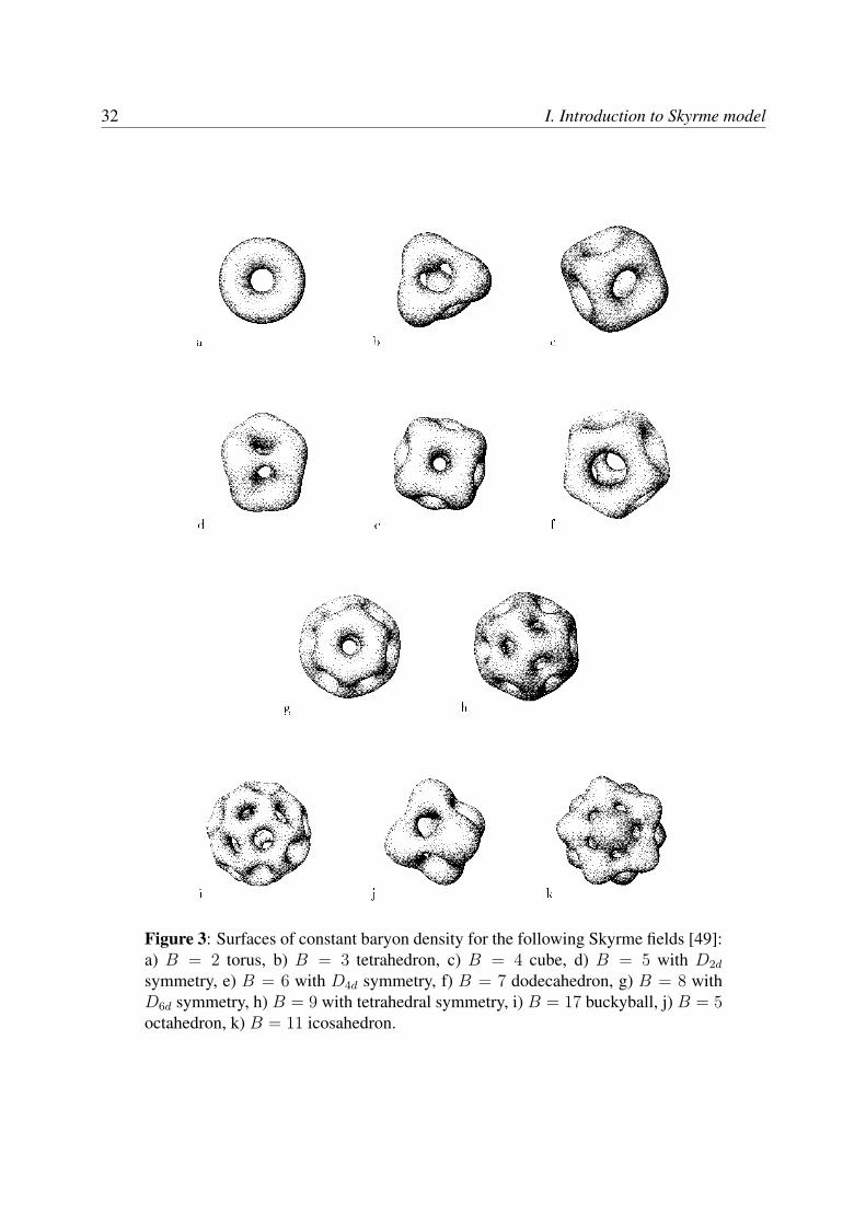
1 from the radial strain eigenvalue.The Skyrme field baryon density contours will therefore look like a polyhedron with holes inthe directions given by the zeros of W , and there will be 2N − 2 of such holes. This structureis seen in all the plots shown in Fig. 3. For example, the B = 7 skyrmion having twelve holesarranged at the face centres of a dodecahedron.

A rational map, R : S2 7→ S2, is invariant (or symmetric) under a subgroup G ⊂ SO(3) ifthere is a set of Möbius transformation pairs {g, Dg} with g ∈ G acting on the domain S2 andDg acting on the target S2, such that

R(g(z)) = DgR(z). (I.4.15)

The transformations Dg should represent G in the sense that Dg1Dg2 = Dg1g2 . Both g and Dg

will in practice be SU(2) matrices. For example, g(z) can be expressed as g(z) = (αz +β)/(−βz + α) with |α|2 + |β|2 = 1. Replacing (α, β) by (−α,−β) has no effect, so g iseffectively in SO(3). The same is true for Dg.

Some rational maps possess an additional symmetry of reflection or inversion. The transfor-mation z 7→ z is a reflection, whereas z 7→ −1/z is the antipodal map on S2, or inversion.

For N = 1 the hedgehog map is R(z) = z. It is fully O(3) invariant, since R(g(z)) = g(z)for any g ∈ SU(2) and R(−1/z) = −1/R(z). This map gives the standard exact hedgehogskyrmion solution (I.3.34) with the usual profile function F (r) .

A general map of degree two is of the form

R(z) =αz2 + βz + γ

λz2 + µz + ν. (I.4.16)

Lets impose the twoZ2 symmetries z 7→ −z and z 7→ 1/z which generate the viergruppe of 180◦

rotations about all three Cartesian axes. The conditions R(−z) = R(z) and R(1/z) = 1/R(z)restrict R to the form

R(z) =z2 − a

−az2 + 1. (I.4.17)

By a target space Möbius transformation, we can bring a to lie in the interval −1 ≤ a ≤ 1,with the map degenerating at the endpoints. Further, a 90◦ rotation, z 7→ iz, reverses the sign ofa. The maps (I.4.17) have three reflection symmetries in the Cartesian axes, which are manifestwhen a is real. For example, R(z) = R(z) when a is real. A baryon density plot for thisconfiguration is shown in Fig. 3a.


A subset of the degree three rational maps N = 3 has symmetry Z2 × Z2, realized by therequirements R(−z) = −R(z) and R(1/z) = 1/R(z). The first condition implies that thenumerator of R is even in z and the denominator is odd, or vice versa. Imposing the secondcondition as well gives maps of the form

R(z) =

√3az2 − 1

z(z2 −√3a)(I.4.18)

with a complex. The inclusion of the factor√

3 is for a convenience. The parameter space ofthese maps should be thought of as a Riemann sphere with a complex coordinate a. The rationalmap degenerates for three values of a, namely a = ∞ and a = ±1/

√3. A slightly subtler

symmetry occurs if a is imaginary.The Wronskian of maps having form (I.4.18) is

W (z) = −√

3a(z4 +√

3(a− a−1)z2 + 1). (I.4.19)

Note that for a = ±i, W is proportional to a tetrahedral Klein polynomial [67]. If a = 1, W hasa square symmetry, but the rational map does not have as much symmetry as this (see Fig. 3b).

The minimal energy skyrmion with B = 4 has octahedral symmetry, and there is a uniqueoctahedrally symmetric N = 4 monopole. The octahedrally symmetric rational map of degreefour can be embedded in a one parameter family of tetrahedrally symmetric maps

R(z) = cz4 + 2

√3iz2 + 1

z4 − 2√

3iz2 + 1, (I.4.20)

where c is real. The numerator and the denominator are tetrahedrally symmetric Klein poly-nomials, so R is invariant up to a constant factor under any transformation in the tetrahedralgroup.

The Wronskian of the map (I.4.20) is proportional to z(z4 − 1) for all values of c. This is theface polynomial of a cube, with faces in the directions 0, 1, i,−1,−i,∞ (i.e. the directions ofthe Cartesian axes). It allows to understand why the baryon density vanishes in these directions,and hence why the skyrmion has a cubic shape, with its energy concentrated on the vertices andthe edges of a cube (see Fig. 3c).

For N = 5 there is a family of rational maps with two real parameters, with the generic maphaving the D2d symmetry, but having higher symmetry at special parameter values [68].

The family of these maps is

R(z) =z(z4 + bz2 + a)

az4 − bz2 + 1(I.4.21)

with a and b real. The two generators of the D2d symmetry are realized as R(i/z) = i/R(z) andR(−z) = −R(z).

The map R(z) = z(z4 − 5)/(−5z4 + 1) has the Wronskian

W (z) = −5(z8 + 14z4 + 1), (I.4.22)

which is proportional to the face polynomial of an octahedron. N = 5 baryon density plot isshown in Fig. 3d.


a b cd e f

g hi j k

Figure 3: Surfaces of constant baryon density for the following Skyrme fields [49]:a) B = 2 torus, b) B = 3 tetrahedron, c) B = 4 cube, d) B = 5 with D2d

symmetry, e) B = 6 with D4d symmetry, f) B = 7 dodecahedron, g) B = 8 withD6d symmetry, h) B = 9 with tetrahedral symmetry, i) B = 17 buckyball, j) B = 5octahedron, k) B = 11 icosahedron.

5. Generalization of the Skyrme model 33

The skyrmions with B = 6 and B = 8 both have extended cyclic symmetry. For B = 6, thedesired symmetry is D4d. D4 is generated by z 7→ iz and z 7→ 1/z. The rational maps

R(z) =z4 + ia

z2(iaz4 + 1)(I.4.23)

have this symmetry, since R(iz) = −R(z) and R(1/z) = 1/R(z). If a is real R(eiπ/4z) = iR(z)and the rational maps have D4d symmetry. The Skyrme field has a polyhedral shape consistingof a ring of eight pentagons capped by squares above and below (see Fig. 3e).

For B = 8, the symmetry is D6d. D6 is generated by z 7→ eiπ/3z and z 7→ i/z. The rationalmaps

R(z) =z6 − a

z2(az6 + 1)(I.4.24)

have this symmetry. If a is real they have D6d symmetry. The polyhedral shape is now a ring oftwelve pentagons capped by hexagons above and below (see Fig. 3g).

The N = 7 case is similar to the cases N = 6 and N = 8, but the skyrmion has a dodecahedralshape (see Fig. 3f). A dodecahedron is a ring of ten pentagons capped by pentagons above andbelow.

Imposing the tetrahedral symmetry on degree nine maps they obtains the one real parameterfamily. The Skyrme field has a polyhedral shape consisting of four hexagons centered on thevertices of a tetrahedron, linked by four triples of pentagons (see Fig. 3h).

The skyrmion with B = 11 have the icosahedral symmetry. This icosahedral configuration isshown in Fig. 3k.

A highly symmetric configuration case is at B = 17, where it has been conjectured that theskyrmion has the icosahedrally symmetric, buckyball structure of carbon 60. The polyhedrondoes indeed have the buckyball form (see Fig. 3i), consisting of twelve pentagons, each sur-rounded by five hexagons, making a total of 32 polygons.

5. Generalization of the Skyrme model

By looking at the Skyrme model as a low energy effective theory from QCD in the limit in whichthe number of colours Nc is large, one finds that the Skyrme field takes values in SU(Nf), whereNf is the number of flavours of light quarks. In previous sections we have only considered thecase of Nf = 2, which is physically the most relevant since the up and down quarks are almostmassless, and the SU(2) flavour symmetry between up and down quarks is only weakly brokenin nature. A model with the SU(3) flavour symmetry, allowing for the strange quark, shouldhave appropriate additional symmetry breaking terms to take into account the higher mass ofthe strange quark. This model is also a reasonable approximation. It allows to study the strangebaryons and nuclei within the Skyrme model. The basic fields now describe pions, kaons, andthe eta meson. There is still just one topological charge, identified as the baryon number. In theabsence of any symmetry breaking mass terms, the three flavour Skyrme Lagrangian is given bythe usual expression (I.3.21), however U ∈ SU(3). There is also a Wess-Zumino term, whichwill be discussed in next section. It is important only in the quantization of skyrmions.

Solutions of the SU(3) model can be obtained by embedding the SU(2) skyrmions, and currentevidence suggests that these are the minimal energy solutions at each charge. However, there are


also solutions which do not correspond to the SU(2) embeddings. Although they have energiesslightly higher than the embedded skyrmions, they are still low energy configurations. Thissymmetries are very different from the SU(2) solutions.

An example of a non-embedded solution is the dibaryon of Balachandran et al. [4], which isa spherically symmetric solution with B = 2. Explicitly, the Skyrme field is given by

U(x) = exp

{iF1(r)Λ · x + iF2(r)

((Λ · x)2 − 2

3· 13

)}, (I.5.25)

where Λ is a triplet of SU(3) matrices generating SO(3) and F1(r), F2(r) are real profile func-tions satisfying the boundary conditions F1(0) = F2(0) = π and F1(∞) = F2(∞) = 0.Substituting this ansatz into the Skyrme Lagrangian density (I.3.21) leads to two coupled ordi-nary differential equations for F1(r) and F2(r). Solving these numerically yields an energy littlehigher than the energy of the embedded SU(2) rational map ansatz (I.4.17) of charge 2.

A different generalization of model is the Skyrme model constructed on a 3-sphere, in whichthe domain R3 is replaced by S3

L, the 3-sphere of radius L, but the Skyrme field is still a mapto the target space SU(2). The baryon number is the degree of U . This generalization has beenstudied in Ref. [69], and in a more geometrical context in Ref. [70]. By taking the limit L →∞the Euclidean model is recovered, but it is possible to gain some additional understanding ofskyrmions by first considering finite values of L.

Let µ, z be coordinates on S3L, with µ being the polar angle (the co-latitude) and z denoting the

Riemann sphere coordinate on the 2-sphere at polar angle µ. Take F , R to be similar coordinateson the unit 3-sphere S3

1, which we identify with the target manifold SU(2).In general, a static field is given by functions F (µ, z, z) and R(µ, z, z). To find the B = 1

skyrmion we consider an analogue of the hedgehog field, an SO(3)-symmetric map of the form

F = F (µ), R = z, (I.5.26)

whose energy is

E =1

3π

∫ π

0

(L sin2 µ

(F ′2 +

2 sin2 F

sin2 µ

)+

sin2 F

L

(sin2 F

sin2 µ+ 2F ′2

))dµ. (I.5.27)

Among these maps there is the 1-parameter family of degree 1 conformal maps defined by

tanF

2= ea tan

µ

2, (I.5.28)

where a is a real constant. These may be pictured as a stereographic projection from S3L to R3,

followed by a rescaling by ea, and then by an inverse stereographic projection from R3 to S31.

Substituting the expression (I.5.28) into the energy (I.5.27), and performing the integral gives

E =L

1 + cosh a+

cosh a

2L. (I.5.29)

If a = 0 then (I.5.28) is the identity map with energy

E =1

2

(L +

1

L

). (I.5.30)

6. The Wess-Zumino term 35

Note that if L = 1 then E = 1, so the Bogomolny bound is attained.In the Euclidean limit L →∞ the radial variable should be identified as the combination r =

Lµ, in which case the expression for the energy (I.5.27) takes the form of the standard energyexpression of the classical Skyrme model (I.3.39). On a small 3-sphere the energy density of aB = 1 skyrmion is uniformly distributed over S3

L and the unbroken symmetry group is SO(4).However as the radius of the 3-sphere is increased beyond the critical value of L =

√2 there is

a bifurcation to a skyrmion localized around a point and the chiral symmetry is broken. Thus aphase transition occurs, when one moves from high to low baryon density, with a correspondingbreaking of the chiral symmetry. This may have relevance to the physical issue of whether thequark confinement occurs at the same time as the chiral symmetry breaks when very dense quarkmatter becomes less dense.

If the charge B > 1 the rational map ansatz can be applied again to produce low energySkyrme fields which approximate the minimal energy skyrmions on S3

L [71,72], by taking R(z)to be a degree B rational map and F (µ) is the associated energy minimizing profile function.This produces fields which tend to those of the Euclidean model as L → ∞ and for all cases,this ansatz produces the good energy configurations.

The substitution of the field expressed in terms of pion fields (I.2.4) into the Lagrangian(I.3.21) reveals that the pions are massless. They are Goldstone bosons of the spontaneouslybroken chiraly symmetry. An additional term

Lmass = m2π

∫Tr

(U − 1

)d3x, (I.5.31)

can be included in the Lagrangian of the Skyrme model to make the pions have a mass mπ.After the inclusion of (I.5.31) the skyrmion becomes exponentially localized, in contrast to thealgebraic asymptotic behaviour of the Skyrme field in the massless pion model. This is becausethe modified equation of the hedgehog F (r) function,

F ′′(r)(

1 +2 sin2F (r)

r2

)+ F ′2(r)

sin 2F (r)

r2+

2

rF ′(r)

− sin 2F (r)

r2− sin 2F (r) sin2F (r)

r4−m2

πr sin F = 0. (I.5.32)

has the asymptotic Yukawa-type solution

F (r) ∼ A

re−mπ r. (I.5.33)

Clearly the energy of a single skyrmion with mπ > 0 will be slightly higher than that withmπ = 0, because the pion mass term is positive for all fields.

For higher charge skyrmions, the rational map approach works as before, but the profile func-tion will again be slightly modified, leading to slightly higher energies.

6. The Wess-Zumino term

The three flavor QCD Lagrangian in the chiral limit ( mu = md = ms = 0) is globally invariantunder U(3)L × U(3)R. By Noether’s theorem there are nine conserved vector and axial vector


currents at the classical level [54]. Because of the Adler-Bell-Jackiw anomaly [73,74] the U(l)Asymmetry is explicitly broken at the quantum level. So aside from the anomaly it is believed thatthe chiral symmetry is spontaneously broken through

U(3)L ⊗ U(3)R/U(1)A ≡ SU(3)L ⊗ SU(3)R ⊗ U(1)V → SU(3)V ⊗ U(1)V, (I.6.1)

with the appearance of eight massless Goldstone bosons, that corresponds to the pseudoscalaroctet mesons: π0, π±, η,K0, K0, K±. In the spirit of the large Nc limit, the dynamics of themassless pseudoscalar mesons is dictated by a nonlinear σ-model Lagrangian such as (I.3.18) toleading order where U(x) is an SU(3)-valued field of the form

U(x, t) = exp i

(λa πa(x, t)

fπ

). (I.6.2)

There the λ’s are the ordinary Gell-Mann matrices with the normalization condition Tr(λaλb

)=

2δa,b. Under U(3)L × U(3)R, U(x, t) transforms as follows:

exp(iQL)U(x, t) exp(−iQR), (I.6.3)

where QL,R are the fundamental generators of U(3). Under parity, U(x, t) transforms accordingto (I.3.38), respectively the pseudoscalar character of the octet mesons transforms:

πop πa(x, t)π−1op = πa(−x, t). (I.6.4)

Witten observed [75] that while the nonlinear σ-model (I.3.18) is invariant under globalU(3)L×U(3)R and even under the QCD parity (I.3.38), it exhibits two discrete symmetries whichare redundant with QCD namely

U(x, t) → U(−x, t), (I.6.5a)U(x, t) → U †(x, t). (I.6.5b)

The latters forbid anomalous processes in which an even number of pseudoscalar mesons decayinto an odd number and vice versa. As a remedy Witten proposed to modify the classical equa-tions of motion in the nonlinear σ-model by adding explicitly a U(3)L ⊗ U(3)R invariant termthat breaks the redundant symmetries (I.6.5a) and (I.6.5b) separately while preserving their com-bination i.e. the QCD parity operation (I.3.38). To break explicitly (I.6.5a) while maintainingLorentz invariance requires the totally anti-symmetric Levi-Cevita tensor

1

2f 2

π∂µRµ + λεµναβRµRνRαRβ = 0. (I.6.6)

Under x → −x, we have εµναβ → −εµναβ , ∂µ → ∂µ and Rµ → Rµ, hence

1

2f 2

π∂µRµ − λεµναβRµRνRαRβ = 0. (I.6.7)

Under πa → −πa, we have U(x) → U †(x) and Rµ → Lµ = −URµU†. Since ∂µLµ +

U∂µRµU† = 0, we obtain

1

2f 2

π∂µRµ + λεµναβRµRνRαRβ = 0. (I.6.8)

6. The Wess-Zumino term 37

In other words the redundant symmetries are lifted while their combination (QCD parity) ispreserved.

To proceed to a quantum description starting from the classical field equations (I.6.6) we needthe corresponding action functional. To do that is non trivial since the obvious candidate for theadded term εµναβ Tr (RµRνRαRβ) vanishes identically in (3 + 1) dimensions due to the cyclicproperty of the trace. In fact, the pertinent action functional involves the Wess-Zumino (WZ)term [44] of current algebra, and turns out to be non local in (3 + 1) dimensions.

The solution of the problem raised by Witten [75] is suggested by the solution of a muchsimpler problem of an electron moving on the surface of a unit sphere surrounding a Diracmagnetic monopole [76] . The analogy of the preceding example with the SU(3)L ⊗ SU(3)Rnonlinear σ-model is striking if we notice that for the vanishing magnetic field, the constrainedequation on S2 is invariant under r → −r and t → −t separately. The additional Lorentz forcecreated by the magnetic monopole preserves only the combination r → −r and t → −t. TheLorentz force is the analogue of the anomaly term in (I.6.6), while the geometrical analogue ofthe one-dimensional closed path S1 on S2 is a four-dimensional quasi-sphere S3×S1on S3×S2.

To elucidate these statements it is best to work in the Euclidean space with a compactified timedirection, i.e. R4 = R3×R1 → R3× S1. Finite field configurations yield a compactification ofR3 into S3 and endow the space-time with the topology of a quasi sphere S3×S1. The latter canbe thought of as the boundary of a five-dimensional manifold D5

D+5 = S3 × S1 × [0, 1], (I.6.9a)

D−5 = S3 × S1 × [−1, 0], (I.6.9b)

where we have used a decomposition of S3. The SU(3) field U(x) acts as a mapping from S3×S1

onto SU(3) whose group manifold is isomorphic to S5 × S3 by Bott’s theorem [77]. In analogywith the U(1) monopole where the action associated to the Lorentz force is a U(1) invariant onthe boundaries D±

2 , the action functional corresponding to the anomaly term in (I.6.6) shouldbe sought as an SU(3)L × SU(3)R invariant on D±

5 . To achieve this the SU(3) map U(x) fromS3 × S1 onto SU(3) should be extended to a map U(x) from D±

5 onto SU(3). Since

(S3 × S2, S5 × S3

) ∼ (S5, S5) ∼ π5(S5) ∼ Z, (I.6.10)

by De-Rham’s theorem [78] there must exist a topologically invariant and closed 5-form ω05 on

S5, such that ∫

S5

ω05 =

∫

S5

d5xQ05 = 2π. (I.6.11)

There Q05 is the Chern-Pontryagin density associated to π5(S5) ∼ Z. To construct an explicit

form of the pertinent isomorphism: π5(S5) → Z, we can use a straightforward generalization ofthe proper construction that led to (I.3.21). In particular, we have

Q05 =

i

240π2ε0µαβγδ Tr

(RµRαRβRγRδ

). (I.6.12)

Its corresponding closed 5-form ω05 is exact. The normalization in (I.6.12) is obtained by first

using a polar parametrization of S5 which yields 2π/5!A5, with A5 = π3 being the surface of


S5 and then making the substitution φ0 = 1 and ∂µφk ∼ iRk

µ, k = 1, 2, 3, 4, 5 for any subset ofSU(3). Indeed, if we define the 1-form α = Rµdxµ, then

ω05 =

i

240π2Tr

(α5

), (I.6.13)

where the wedge product has been omitted for convenience.The Wess-Zumino Lagrangian associated to the anomaly term in (I.6.6) can be cast in the

formLWZ = +λ

∫

D+5

ω05 = −λ

∫

D−5

ω05, λ ∈ R, (I.6.14)

where D±5 are the complementary discs defined in (I.6.9). To summarize:

• LWZ is SU(3)L ⊗ SU(3)R invariant.

• LWZ is topologically invariant, since ω05 is closed.

• LWZ depends only on the space-time boundary ∂µD5 = S3 × S1, since ω05 is locally exact.

In terms of (I.6.14), the modified nonlinear σ-model action is

S± = −f 2π

4d4x Tr

(RµRµ

)± iλ

240π2

∫

D±5

d5xεµαβγδ Tr(RµRαRβRγRδ

). (I.6.15)

The contour ambiguity in (I.6.15) can be resolved if one requires the generating functional (andhence the exponential factors exp(iS±)) to be contour independent. This is fulfilled if and onlyif exp(iS+) = exp(iS−), i.e.

λ

(∫

D+5

ω05 +

∫

D−5

ω05

)= λ

∫

D+5 ∪D−5

ω05 = λ

∫

S3×S2

ω05 ≡ 2πλ ≡ 2πn, λ = n = integer. (I.6.16)

This shows that λ is topologically quantized. When analyzed in the context of QCD, this quan-tization is of fundamental relevance to the skyrmion.

The action (I.6.15) can be expresed in a non local form in the ordinary space-time. Indeed, tothe leading order in the pseudoscalar fields φ(x) = λaπa/fπ, the Wess-Zumino term in (I.6.15)becomes

LWZ =± n

240π2

∫

D±5

d5xεµναβγ Tr(∂µφ∂νφ∂αφ∂βφ∂γφ

)+ ...

=n

240π2

∫

∂D5=S3×S1

dΣµεµναβγ Tr

(∂µφ∂νφ∂αφ∂βφ∂γφ

)+ ..., (I.6.17)

where Stoke’s theorem was used. The expression (I.6.17) was originally investigated by Wessand Zumino [44] in the context of the effective Lagrangians.

The phenomenological implications of the topological quantization of the WZ term LWZ arerelevant to low energy observables. At low energy, it provides the canonical link between QCD

7. Quantization of model 39

and chiral effective descriptions based on the nonlinear σ-model (see I.2. section). In the contextof the QCD, the number n is identified with the number of colors, i.e. n ≡ Nc. Finally, theWess-Zumino action can be written as

SWZ(U(x)) = − Nc

240π2

∫

D5

d5xεµναβγ Tr(RµRνRαRβRγ

). (I.6.18)

In this equation it is understood that the pion field U(x) is continued without singularities fromthe physical 4-dim space-time to a fifth dimension, so that the physical space-time serves as bor-der of the 5-dim disk. Actually, it can be shown that the integrand in (I.6.18) is a full derivative,consequently the Wess-Zumino action (I.6.18) does not depend on a concrete way one continuesthe pion field inside the disk [79].

The Wess-Zumino term does not contribute to the classical energy, but it plays an importantrole in the quantum theory. Its introduction breaks the time reversal and parity symmetries ofthe model down to the combined symmetry operation: t → −t, x → −x, U → U †, whichappears to be realized in nature, unlike these individual symmetry operations.

7. Quantization of modelQuantization is a vital issue for skyrmions. It is more important than for the other solitons, be-cause skyrmions are supposed to model physical baryons and nuclei, and a single baryon is aspin half fermion. Quantization of skyrmions may raise some questions, because the Skyrmemodel it is not a fundamental field theory, but rather a classical model that results from takingthe limit of such a theory, including only some degrees of freedom of the original theory. Ne-vertheless, there is a rich experience from the nonrelativistic many-body problems, for example,from nuclear physics [80], suggesting the validity of such an approach for the study of collectiveproperties at low energies.

To determine whether a skyrmion should be quantized as a fermion we can compare theamplitudes for the processes in which a skyrmion remains at rest for some long time t, and inwhich the skyrmion is slowly rotated through an angle 2π during this time. The sigma model andthe Skyrme terms in the action do not distinguish between these two processes, since they involvetwo or more time derivatives. Since the Wess-Zumino term is only linear in time derivatives, itcan distinguish them. In fact it results in the amplitudes for these two processes differing by afactor (−1)Nc , which shows that the skyrmion should be quantized as a fermion when Nc is odd,and in particular, in the physical case Nc = 3 [3, 75].

For Nc = 2 the above analysis does not apply, since the Wess-Zumino term vanishes foran SU(2)-valued field. To determine the appropriate quantization of an SU(2) skyrmion onemay follow the approach of Finkelstein and Rubinstein [81], who showed that it is possible toquantize a soliton as a fermion by lifting the classical configuration space to its simply connectedcovering space. In the SU(2) Skyrme model, this is a double cover for any value of B.

A practical, approximate quantum theory of skyrmions is achieved by a rigid body quanti-zation of the spin and isospin rotations. Vibrational modes whose excited states usually haveconsiderably higher energy are ignored. For the B = 1 skyrmion, this quantization was carriedout by Adkins, Nappi and Witten [5], who showed that the lowest energy states (compatiblewith the Finkelstein-Rubinstein constraints) have spin half and isospin half, and may be identi-fied with the states of a proton or neutron.


The quantization of the B = 2 skyrmion was first discussed by Braaten and Carson [82], usinga rigid body quantization. Their analysis was extended by Leese, Manton and Schroers [83], whoalso allowed the toroidal skyrmion to break up in the direction of the lowest vibrational mode,which corresponds to the attractive channel. Both calculations found that the lowest energyquantum state has isospin zero and spin 1, as expected for the deuteron. The second calculationgets closer to the usual physical picture of the deuteron as a rather loose proton-neutron boundstate.

The quantization for higher charge skyrmions has been performed [82, 84–88] for chargesB ≤ 8, and gives the correct quantum numbers (spin, isospin and parity) for the experimentallyobserved ground states of nuclei in all cases except B = 5 and B = 7. A further study, makinguse of the topological properties of the space of rational maps, has allowed an extension of thisanalysis up to B = 22 [89]. The fact that some results do not agree with the experimental datais probably due to the restricted zero mode quantization, which does not allow any vibrationalor deformation modes.

In our work we use the quantization in the “zero modes” or “collective coordinate” ap-proach [5, 9]. As general, the construction of quantum theory passes three steps: the classicalLagrangian leads to the classical Hamiltonian which is modified to the quantum Hamiltonian.The quantization in the collective coordinate approach slightly modifies this sequence. It startsfrom the quantum Lagrangian from the outset. By the quantum Lagrangian we mean that thedynamical coordinates qi and their time derivatives (velocities) qi do not commute. The explicitcommutation relations are not defined in the begining. These relations are extracted from thestandard commutation relations [qi, pj] after we pass to the quantum Hamiltonian (and definethe canonical momenta pj). It can be shown that this modified formalism [90–92] leads to aconsistent quantum description.

The results of the modified and usual quantization sequences are usually different. Non-commuting quantum variables will generate additional terms while passing from the quantumLagrangian to the quantum Hamiltonian. These terms are lost when we impose the canonicalcommutation relations after the Hamiltonian is obtained. This problem is similar to the operatorordering problem.

Following [93] we utilize the following detailed quantization sequence:1. Introduce the quantum collective coordinates matrix A

(q(t)

)(I.7.1). They are quantum in

the sense that the dynamical variables q(t) and the time derivatives q(t) do not commute.2. Make the Lagrangian quantum.3. Following the method described in [90–96] pass to the quantum Hamiltonian.4. Solve the integro-differential equation for the quantum profile function F (r).Another important point is symmetry properties of the classical Lagrangian and the quantum

Hamiltonian derived from it. There are quantization methods (for example, the general covariantHamiltonian method [97]) preserving original classical Lagrangian symmetries. The symmetricWeyl ordering of the operators q and p (used in the work), however, cannot avoid a risk that thequantum Hamiltonian has a chiral symmetry breaking term [98] .

According to G.S. Adkins et al. [5] we employ the collective rotational coordinates to separatethe variables which depend on the time and spatial coordinates

U(x, q(t)

)= A

(q(t)

)Ucl(x)A†(q(t)), A

(q(t)

) ∈ SU(Nc). (I.7.1)

The real independent parameters q(t) =(q1(t), q2(t), ..., qk(t)

), where k = dim(SU(Nc)), are

the dynamical quantum variables – the skyrmion rotation (Euler) angles in the internal space

7. Quantization of model 41

SU(Nc) = diag(SU(Nc)L ⊗ SU(Nc)R

)but not in the geometric space. The skyrmion remains

static in the geometric space.Quantum fluctuations near the classical solution can be put into two different classes. Namely,

the fluctuation modes which are generated by the action or the Hamiltonian symmetries and themodes orthogonal to the symmetric one. Symmetric fluctuation modes are of primary impor-tance in the quantum description because the infinitely small energy perturbation can lead toreasonable deviations from the classical solution. As a consequence, the collective rotation ma-trices A(t) and A†(t) in (I.7.1) are not required to be small (i.e. close to the identity matrix) [62].

We shall consider the Skyrme Lagrangian quantum mechanically ab initio [9, 93]. The gene-ralized coordinates q(t) and velocities q(t) then satisfy the commutation relations

[qk, ql

]= −igkl(q). (I.7.2)

Here the tensor gkl(q) is a function of the generalized coordinates q only. Its explicit form isdetermined after the quantization condition has been imposed. The tensor gkl is symmetric withrespect to an interchange of the indices k and l as a consequence of the commutation relation[qk, ql] = 0. Indeed, differentiation of the relation gives [qk, ql] = [ql, qk], from what it followsthat gkl is symmetric. The commutation relation between a generalized velocity component qk

and an arbitrary function G(q) is given by

[qk, G(q)

]= −i

∑r

gkl(q)∂

∂qlG(q). (I.7.3)

We shall employ the Weyl ordering for the noncommuting operators q and G(q) through

(∂tG(q))W =1

2

{ql,

∂G(q)

∂ql

}, (I.7.4)

which is a consequence of application of the Newton-Leibnitz rule to the Taylor series expansionof the arbitrary function G(q):

G(q) = G(q0) + G′(q)∣∣∣q=q0

q +1

2G′′(q)

∣∣∣q=q0

q2 + · · · . (I.7.5)

Indeed,

(∂tq2)W = ∂t(q q) = qq + qq =

1

2

{q,

d(q2)

dq

}, (I.7.6a)

(∂tq3)W = ∂t(q q q) = qq2 + qqq + q2q =

3

2(qq2 + q2q) =

1

2

{q,

d(q3)

dq

}, (I.7.6b)

. . . . . . . . . . . . . . . .

(∂tqn)W = ∂t (q . . . q)︸︷︷︸

n

= qqn−1 + · · ·+ qn−1q =1

2

{q,

dqn

dq

}. (I.7.6c)

The operator ordering is fixed by the form of the classical Lagrangian and no further ambiguityassociated with it appears at the level of the Hamiltonian. In order to find the explicit form ofgkl(q) one can substitute (I.7.1) into the expression of the Lagrangian density (I.3.21) and keeponly the terms quadratic in velocities


L(q, q, F ) =1

N

∫L(

x, q(t), q(t), F (r))r2d3r

=1

2qkgkl(q)q

l +[(q)0– order term

], (I.7.7)

where a normalization factor N is introduced in the Lagrangian in order to ensure the baryonnumber 1 for the spherically symmetric skyrmion case. After the determination of the metrictensor gkl(q), we find the soliton moments of inertia and the explicit expression of the collectivecoordinates A†A. By using these expressions and a set of auxiliary expressions which shownin appendices A, B and C, the complete expression of the Skyrme model Lagrangian density isobtained. Later special techniques are applied to construct the effective Hamiltonian.

II. Canonical quantization of the SU(3)Skyrme model in a generalrepresentation

Both the SU(2) and SU(3) Skyrme versions of the model have been quantized canonically inRefs. [9, 93, 99] in the collective coordinate formalism. The canonical quantization procedureleads to quantum corrections to the skyrmion mass, which restore the stability of the soliton so-lutions that is lost in the semiclassical quantization. This method has subsequently been genera-lized to the unitary fields U(x,t) that belong to the general representations of the SU(2) [11–13],along with a demonstration that the quantum corrections, which stabilize the soliton solutions,are representation dependent.

The aim of this chapter is to extend the canonically quantized Skyrme model to the generalirreducible representations (irrep) of SU(3). The motivation is the absence of any a priori reasonto restrict the collective chiral models to the fundamental representation of the group. The focushere is on the mathematical aspects of the model, and on the derivation of both the Hamiltoniandensity and the Hamiltonian, in order to elucidate their representation dependence. The possiblephenomenological applications both in hyperon and hypernuclear phenomenology as well as inthe Skyrme model description of the quantum Hall effect [6] and Bose-Einstein condensates [7],are not elaborated.

Similarly to the SU(2) case, the solutions to the SU(3) Skyrme model depend in an essentialway on the dimension. Remarkably the Wess-Zumino term vanishes in all self-adjoint irrepsof SU(3), as it is proportional to the cubic Casimir operator CSU(3)

3 in the collective coordinatemethod of separation of the dependence on space and time variables. In the self adjoint irrepsthe symmetry breaking mass term in the model reduces to the SU(2) form.

1. Definitions for the unitary SU(3) soliton field

The unitary field U(x, t) is defined for general irreps (λ, µ) of SU(3) in addition to the fundamen-tal representation (1, 0). The related Young tableaux are denoted [λ1, λ2, λ3], where λ = λ1−λ2,µ = λ2− λ3. A group element is specified by eight real parameters αi(x, t). The unitary field isexpressed in the form of the Wigner D matrices for SU(3) in (λ, µ) irrep as

U(x, t) = D(λ,µ)(αi(x, t)). (II.1.1)

The one-form of the unitary field belongs to the Lie algebra of SU(3). The one-forms may bedetermined by the functions C

(Z,I,M)i (α) and C

′(Z,I,M)i (α). Their explicit expressions depend on

43

44 II. Canonical quantization of the SU(3) Skyrme model in a general representation

the specific group parametrization

∂iUU † =

(∂

∂αiU

)U † = C

(Z,I,M)i (α)

⟨ ∣∣∣ J(1,1)(Z,I,M)

∣∣∣⟩

,

U †∂iU = U † ∂

∂αiU = C

′(Z,I,M)i (α)

⟨ ∣∣∣ J(1,1)(Z,I,M)

∣∣∣⟩

, (II.1.2)

The basis states of irrep (1,1) are specified by the parameters isospin I , and its projections Mand Z, which is related to the hypercharge as Y = −2Z.

The parametrization for the SU(3) model, and the expressions of the differential Casimiroperator in terms of the Euler angles, have been proposed by Yabu and Ando [100]. In contrastto their approach, for simplicity, we do not determine the specific parametrization and use thegeneral properties of the functions C

(Z,I,M)i (α) (see B.1). The SU(3) generators are defined as

components of the irreducible tensors (1, 1) and may be expanded in terms of the Gell-Mangenerators Λk:

Λ1 =√

2(J

(1,1)0,1,−1 − J

(1,1)0,1,1

); J

(1,1)0,1,1 =− 1

2√

2(Λ1 + iΛ2) ;

Λ2 = i√

2(J

(1,1)0,1,−1 + J

(1,1)0,1,1

); J

(1,1)0,1,−1 =

1

2√

2(Λ1 − iΛ2) ;

Λ3 = 2J(1,1)0,1,0 ; J

(1,1)0,1,0 =

1

2Λ3;

Λ4 =√

2(J

(1,1)

− 12, 12, 12

+ J(1,1)12, 12,− 1

2

); J

(1,1)

− 12, 12, 12

=1

2√

2(Λ4 + iΛ5) ;

Λ5 =− i√

2(J

(1,1)

− 12, 12, 12

− J(1,1)12, 12,− 1

2

); J

(1,1)12, 12,− 1

2

=1

2√

2(Λ4 − iΛ5) ;

Λ6 =√

2(J

(1,1)

− 12, 12,− 1

2

− J(1,1)12, 12, 12

); J

(1,1)

− 12, 12,− 1

2

=1

2√

2(Λ6 + iΛ7) ;

Λ7 =− i√

2(J

(1,1)

− 12, 12,− 1

2

+ J(1,1)12, 12, 12

); J

(1,1)12, 12, 12

=− 1

2√

2(Λ6 − iΛ7) ;

Λ8 =− 2J(1,1)0,0,0 ; J

(1,1)0,0,0 =− 1

2Λ8. (II.1.3)

The Λi matrices are hermitian Λ†i = Λi. Although the generators (II.1.3) are non-hermitian(J

(1,1)(Z,I,M)

)†= (−1)Z+MJ

(1,1)(−Z,I,−M), their commutation relations nevertheless have a simple form

[J

(1,1)(Z′,I′,M ′), J

(1,1)(Z′′,I′′,M ′′)

]= −

∑

(Z,I,M)

√3[

(1,1) (1,1) (1,1)a

(Z′,I′,M ′) (Z′′,I′′,M ′′) (Z,I,M)

]J

(1,1)(Z,I,M) . (II.1.4)

For the specification of the basis states in a general irrep (λ, µ) the parameters (z, j, m) areemployed. The hypercharge is y = 2

3(µ − λ) − 2z. The basis state parameters satisfy these

inequalities:

j −m ≥0 , j − z ≥ 0 ,

j + m ≥0 , j + z ≥ 0 ,

λ + z − j ≥0 , µ− z − j ≥ 0 , (II.1.5)

1. Definitions for the unitary SU(3) soliton field 45

where the values on the left hand sides are integers. The generators (II.1.3) act on the basis statesas follows:

J(1,1)(0,0,0)

∣∣∣∣(λ, µ)

z, j,m

⟩= −

√3

2y

∣∣∣∣(λ, µ)

z, j, m

⟩, J

(1,1)(0,1,−1)

∣∣∣∣(λ, µ)

z, j,m

⟩=

√12(j+m)(j−m+1)

∣∣∣∣(λ, µ)

z, j, m− 1

⟩,

J(1,1)(0,1,0)

∣∣∣∣(λ, µ)

z, j,m

⟩= m

∣∣∣∣(λ, µ)

z, j,m

⟩, J

(1,1)(0,1,1)

∣∣∣∣(λ, µ)

z, j,m

⟩= −√

12(j−m)(j+m+1)

∣∣∣∣(λ, µ)

z, j, m + 1

⟩,

J(1,1)

(− 12, 12, 12)

∣∣∣∣(λ, µ)

z, j, m

⟩=

√(λ+z−j)(µ−z+j+2)(j−z+1)(j+m+1)

2(2j+1)(2j+2)

∣∣∣∣(λ, µ)

z − 12, j + 1

2,m + 1

2

⟩

−√

(λ+z+j+1)(µ−z−j+1)(j+z)(j−m)4j(2j+1)

∣∣∣∣(λ, µ)

z − 12, j − 1

2,m + 1

2

⟩,

J(1,1)

( 12, 12,− 1

2)

∣∣∣∣(λ, µ)

z, j, m

⟩= −

√(λ+z+j+2)(µ−z−j)(z+j+1)(j−m+1)

2(2j+1)(2j+2)

∣∣∣∣(λ, µ)

z + 12, j + 1

2,m− 1

2

⟩

+√

(λ+z−j+1)(µ−z+j+1)(j−z)(j+m)4j(2j+1)

∣∣∣∣(λ, µ)

z + 12, j − 1

2,m− 1

2

⟩,

J(1,1)

(− 12, 12,− 1

2)

∣∣∣∣(λ, µ)

z, j, m

⟩=

√(λ+z−j)(µ−z+j+2)(j−z+1)(j−m+1)

2(2j+1)(2j+2)

∣∣∣∣(λ, µ)

z − 12, j + 1

2,m− 1

2

⟩

+√

(λ+z+j+1)(µ−z−j+1)(j+z)(j+m)4j(2j+1)

∣∣∣∣(λ, µ)

z − 12, j − 1

2,m− 1

2

⟩,

J(1,1)

( 12, 12, 12)

∣∣∣∣(λ, µ)

z, j, m

⟩= −

√(λ+z+j+2)(µ−z−j)(j+z+1)(j+m+1)

2(2j+1)(2j+2)

∣∣∣∣(λ, µ)

z + 12, j + 1

2,m + 1

2

⟩

−√

(λ+z−j+1)(µ−z+j+1)(j−z)(j−m)4j(2j+1)

∣∣∣∣(λ, µ)

z + 12, j − 1

2,m + 1

2

⟩.

(II.1.6)

The basis states are chosen such that the generators J(1,1)(0,1,0) and J

(1,1)(0,0,0), as well as the Casimir

operator of the SU(2) subgroup CSU(2) =∑

(−1)MJ(1,1)(0,1,M)J

(1,1)(0,1,−M), are diagonal and thus pro-

vide a labelling of the basis states

CSU(2)

∣∣∣∣(λ, µ)

z, j, m

⟩= j(j + 1)

∣∣∣∣(λ, µ)

z, j, m

⟩. (II.1.7)

The calculation method of the Clebsch-Gordan (CG) coefficients of SU(3), which were usedfor derivation of the SU(3) Skyrme model in a general representation, was used from the workof J.G. Kuriyan et al. [101]. An algebraic tabulation of the CG coefficients which occur in thereduction of the direct product (λ, µ)⊗(1, 1) into irreducible representations is made. The phaseconvention is an explicitly stated generalization of the well-known Condon and Shortley phaseconvention for SU(3).

The CG coefficients factorize [102, 103] according to[

(1,1) (1,1) (1,1)γ

Z′,I′,M ′ Z′′,I′′,M ′′ Z,I,M

]=

[(1,1) (1,1) (1,1)γ

(Y ′)Z′,I′ (Y ′′)Z′′,I′′ (Y )Z,I

] [I′ I′′ I

M ′ M ′′ M

], (II.1.8)

where the second factor on right hand side of the equation refers to the isospin SU(2) subgroupof SU(3), and the first factor (isoscalar factor) is independent of M ′, M ′′ and M . The label γ in


the CG coefficient takes two values γ = 1 and 2. The first value denotes the antisymmetrical CGcoefficient (sometimes it is labelled by index a) while the second value denotes the symmetricalCG coefficient (sometimes it is labelled by the index s). Hence, the CG coefficient of SU(2)being well-known, we need to tabulate only the isoscalar factors. Some isoscalar factors both forthe symmetrical and antisymmetrical representation, and their properties are shown in AppendixB.

2. The Classical SU(3) Skyrme model

The action of the Skyrme model in SU(3) is taken to have the form

S =

∫d4x(LSk + LSB) + SWZ , (II.2.1)

where LSk is the chirally symmetric Lagrangian density (I.3.21) in which the right chiral currentis defined as

Rµ = (∂µU) U † = ∂µαiC

(Z,I,M)i (α)

⟨ ∣∣∣ J(1,1)(Z,I,M)

∣∣∣⟩

. (II.2.2)

The Greek characters indicate differentiation with respect to the spacetime variables ∂µ ≡ ∂/∂xµ

in the metric diag(ηαβ) = (1,−1,−1,−1). The symmetry breaking term LSB and the Wess-Zumino action SWZ are specified below.

Upon substitution of (II.2.2) into the Skyrme Lagrangian (I.3.21) the classical Lagrangiandensity may be expressed in terms of the group parameters αi as

LSk =3

32Ndim(λ, µ)CSU(3)

2 (λ, µ)

{−f 2

π(−1)A∂µαiC

(A)i (α)∂µαi′C

(−A)i′ (α)

+3

8e2(−1)A∂µα

iC(A1)i (α)∂να

i′C(A2)i′ (α)

× ∂µαi′′C(A3)i′′ (α)∂ναi′′′C

(A4)i′′′ (α)

[(1,1) (1,1) (1,1)a

(A1) (A2) (A)

] [(1,1) (1,1) (1,1)a

(A3) (A4) (−A)

]}. (II.2.3)

At the end of equation (II.2.3), only the SU(3) Clebsch-Gordan coefficients with the antisymmet-ric irrep coupling are included and there is no summation over the irrep multiplicity. The capitalLatin character indices (A) denote the state label (Z, I, M). (−A) denotes (−Z, I,−M) and(−1)A = (−1)Z+M . The dependence on the group irrep appears as an overall factor becauseof the calculation of trace (B.17) where the dimension of the irrep and the quadratic Casimiroperator of SU(3) are included.

The time component of the conserved topological current in the Skyrme model represents thebaryon number density which in terms of the variables αi(x, t) takes the form

B0(x) =1

24π2Nε0ikl Tr

((∂iU) U † (∂kU) U † (∂lU) U †

)

=(−1)A

27√

3π2Ndim(λ, µ)CSU(3)

2 (λ, µ)εabc∂aαiC

(A)i (α)

× ∂bαi′C

(A′)i′ (α)∂cα

i′′C(A′′)i′′ (α)

[(1,1) (1,1) (1,1)a

(A′) (A′′) (−A)

]. (II.2.4)

2. The Classical SU(3) Skyrme model 47

For the classical chiral symmetric Skyrme model the dependence on the irrep is contained inthe overall factor N . The normalization factor

N =1

4dim(λ, µ)CSU(3)

2 (λ, µ) , (II.2.5)

is chosen requiring that the smallest non trivial baryon number equals unity: B =∫

d3xB0(x) =1. The dynamics of the system is independent of the overall factor in the Lagrangian. Thereforein the classical case the Skyrme model defined in an arbitrary irrep is equivalent to the Skyrmemodel in the fundamental representation (1, 0), for which N = 1 .

The classical soliton solution of the hedgehog type for the (λ, µ) irrep of the SU(3) groupmay be expressed as a direct sum of the hedgehog ansatz in the SU(2) irreps [12]. The SU(2)representations embedded in the (λ, µ) irrep are defined by the canonical SU(3) ⊃ SU(2) chain.The hedgehog generalization takes the form

exp i(τ · x)

F (r) → U0

(x, F (r)

)= exp i2

(J

(1,1)(0,1,·) · x

)F (r) =

(λ,µ)∑z,j

⊕Dj(α) , (II.2.6)

where τ are the Pauli matrices and x is the unit vector. The expressions of the Euler angles αof the SU(2) subgroup are shown in (A.12). The normalization factor (II.2.5) ensures that thebaryon number density for the hedgehog skyrmion in a general irrep has the usual form

B0(x) =1

24π2Nε0ikl Tr

((∂iU0) U †

0 (∂kU0) U †0 (∂lU0) U †

0

)

=− 1

2π2

sin2 F (r)

r2F ′(r) . (II.2.7)

With the hedgehog ansatz (II.2.6), and after the renormalization with the factor (II.2.5), theLagrangian density (I.3.21) reduces to the following simple form

Lcl(F (r)

)=−Mcl(F (r)) = −

{f 2

π

2

(F ′2 +

2

r2sin2F

)

+1

2e2

sin2F

r2

(2F ′2 +

sin2F

r2

)}. (II.2.8)

Variation of the classical hedgehog soliton mass leads to standard differential equation for theprofile function F (r).

The SU(3) chiral symmetry breaking term of the Lagrangian density is defined here as

LSB = −MSB = − 1

N

f 2π

4

(m2

0 Tr(U + U † − 2 · 1

)− 2m2

8 Tr((

U + U †) J(1,1)(0,0,0)

)). (II.2.9)

This form is chosen so that it reduces to the mass term of the π, K, η mesons when the unitaryfield U(x, t) = exp{ i

fπϕkΛk} is expanded around the classical vacuum U = 1 :

LSB = −1

2m2

π

(ϕ2

1 + ϕ22 + ϕ2

3

)− 1

2m2

K

(ϕ2

4 + ϕ25 + ϕ2

6 + ϕ27

)− 1

2m2

ηϕ28 + ... . (II.2.10)

For arbitrary irrep the coefficients in the symmetry breaking term can be readily obtained as

m20 =

1

3

(m2

π + 2m2K

), m2

8 =10

3√

3

CSU(3)2 (λ, µ)

CSU(3)3 (λ, µ)

(m2

π −m2K

), (II.2.11)


whereCSU(3)

3 (λ, µ) =1

9(λ− µ)(2λ + µ + 3)(2µ + λ + 3) , (II.2.12)

is the eigenvalue of the cubic Casimir operator of SU(3).For the self adjoint irreps λ = µ the symmetry breaking part of the Lagrangian (II.2.9) is

proportional to m20 = 1

4m2

π only. The Gell-Mann-Okubo mass formula

m2π + 3m2

η − 4m2K = 0 , (II.2.13)

is satisfied in all but the self adjoint irreps.

3. Quantization of the skyrmion

The direct quantization of the Skyrme model leads to rather complicated equations [11] evenin the case of SU(2). Here the collective coordinates for the unitary field U in the (λ, µ) irrepare employed for the separation of the variables, which depend on the temporal and spatialcoordinates

U(x, F (r), q(t)

)= A

(q(t)

)U0

(x, F (r)

)A†(q(t)), A

(q(t)

) ∈ SU(3). (II.3.1)

Because of the form of the ansatz U0 (II.2.6), the unitary field U is invariant under the right U(1)transformation of the A

(q(t)

)= D(λ,µ)(q(t)) matrix, defined as

A(q(t)

) → A(q(t)

)exp βJ

(1,1)(0,0,0) . (II.3.2)

Thus the seven-dimensional homogeneous space SU(3)/U(1), which is specified by seven real,independent parameters qk(t), has to be considered. The mathematical structure of the Skyrmemodel and its quantization problems on the coset space SU(3)/U(1) have been examined by seve-ral authors [35,75,104,105]. The canonical quantization procedure for the SU(3) Skyrme modelin the fundamental representation has been considered by Fujii et al. [99]. Here the attention ison the representation dependence of the model. The Lagrangian (I.3.21) is considered quantummechanically ab initio. The generalized coordinates qk(t) and velocities (d/dt)qk(t) = qk(t)satisfy the commutation relations

[qk, ql

]= −igkl(q) , (II.3.3)

where gkl(q) are functions of qk only. Their form will be determined below. The commutationrelation between a velocity component qk and an arbitrary function of q is given by (I.7.3). Forthe time derivative the usual Weyl ordering (I.7.4) is adopted and the operator ordering is fixedby the form of the Lagrangian (I.3.21).

For the purpose of defining the metric tensor in the Lagrangian we use approximate expres-sions

AA† ≈1

2

{qi, C

(Z,I,M)i (q)

}⟨ ∣∣∣ J(1,1)(Z,I,M)

∣∣∣⟩

, (II.3.4a)

A†A ≈1

2

{qi, C

′(Z,I,M)i (q)

}⟨ ∣∣∣ J(1,1)(Z,I,M)

∣∣∣⟩

. (II.3.4b)

3. Quantization of the skyrmion 49

The ansatz (II.3.1) is then substituted in the Skyrme Lagrangian (I.3.21) following by an inte-gration over the spatial coordinates. The Lagrangian is then obtained in terms of the collectivecoordinates and velocities. For the derivation of the canonical momenta it is sufficient to re-strict the consideration to terms of the second order in the velocities (the terms of the first ordervanish). This leads to

LSk ≈ −∫

drr2

{∑M

(−1)M{

qi, C′(0,1,M)i (q)

}{qi′ , C

′(0,1,−M)i′ (q)

}

× π

3sin2 F

(f 2

π +1

e2

(F ′2 +

1

r2sin2 F

))

+∑Z,M

(−1)Z+M{

qi, C′(Z, 1

2,M)

i (q)}{

qi′ , C′(−Z, 1

2,−M)

i′ (q)}

× π

4(1− cos F )

(f 2

π +1

4e2

(F ′2 +

2

r2sin2 F

))}

≈ 1

2qαgαβ(q, F )qβ +

[(q)0– order terms

]

≈ 1

8

{qα, C ′(A)

α (q)}

E(A)(B)(F ){

qβ, C′(B)β (q)

}+

[(q)0– order terms

], (II.3.5)

the derivation of which is shown in (B.21–B.23).The Lagrangian (II.3.5) is normalized by the factor (II.2.5). The metric tensor takes the form

gαβ(q, F ) = C ′(A)α (q)E(A)(B)(F )C

′(B)β (q), (II.3.6)

whereE(Z,I,M)(Z′,I′,M ′)(F ) = −(−1)Z+MaI(F )δZ,−Z′δI,I′δM,−M ′ . (II.3.7)

Here the soliton moments of inertia are given as integrals over the dimensionless variable r =efπr:

a0(F ) = 0, (II.3.8a)

a 12(F ) =

1

e3fπ

a 12(F ) =

1

e3fπ

2π

∫drr2 (1− cos F )

(1 +

1

4F ′2 +

1

2r2sin2 F

), (II.3.8b)

a1(F ) =1

e3fπ

a1(F ) =1

e3fπ

8π

3

∫drr2 sin2 F

(1 + F ′2 +

1

r2sin2 F

). (II.3.8c)

The canonical momentum, which is conjugate to qβ , is defined as

p(0)β =

∂LSk

∂qβ=

1

2{qα, gαβ} . (II.3.9)

The canonical commutation relations[qα, qβ

]=

[p(0)

α , p(0)β

]= 0, (II.3.10a)

[p

(0)β , qα

]=− iδαβ , (II.3.10b)


then yield the following explicit form for the functions gαβ(q):

gαβ(q) = (gαβ)−1 = C ′α(A)(q)E

(A)(B)(F )C ′β(B)

(q) , (II.3.11)

whereE(Z,I,M)(Z′,I′,M ′)(F ) = −(−1)Z+M 1

aI(F )δZ,−Z′δI,I′δM,−M ′ . (II.3.12)

Note that here E(0)(0)(F ) is left undefined. The summation over the indices (A) denotes sum-mation over the basis states (Z, I, M) of the irrep (1, 1), excluding the state (0, 0, 0). It provesconvenient to introduce the reciprocal function matrix C ′α

(A)(q), the properties of which are de-

scribed in Appendix B. The commutation relations of the momenta (II.3.10b) ensure the choiceof the parameters qα on the manifold SU(3)/U(1) (see [9, 93] ). There is no need for an explicitparameterization of qα at this moment.

Having determined the function gαβ(q) the following explicit expression of A†A is obtained:

A†A =1

2D(λ,µ)(−q)

{qα, ∂αD(λ,µ)(q)

}

=1

2

{qα, C ′(A)

α (q)}⟨ ∣∣∣ J

(1,1)(A)

∣∣∣⟩

− 1

2iC ′α

(A)(q)E(A)(B)(F )C ′β

(B)(q)C

′(K)β (q)C ′(K′)

α (q)⟨ ∣∣∣ J

(1,1)(K) J

(1,1)(K′)

∣∣∣⟩

=1

2

{qα, C ′(A)

α (q)}⟨ ∣∣∣ J

(1,1)(A)

∣∣∣⟩

− 1

2iE(A)(B)(F )C ′β

(B)(q)C

′(0)β (q)

(⟨ ∣∣∣ J(1,1)(0) J

(1,1)

(A)

∣∣∣⟩

+⟨ ∣∣∣ J

(1,1)

(A)J

(1,1)(0)

∣∣∣⟩)

− 3

8iE(A)(B)(F )C ′α

(A)(q)C′(0)α (q)C ′β

(B)(q)C

′(0)β (q)

(λ,µ)∑z,j

⊕ y2 · 1z,j

+i

2a 12(F )

CSU(3)2 (λ, µ) · 1λ,µ + i

(λ,µ)∑z,j

⊕(

CSU(2)(j)

2a1(F )− CSU(2)(j) + 3

4y2

2a 12(F )

)· 1z,j.

(II.3.13)

Here 1λ,µ is the unit matrix in the (λ, µ) irrep of SU(3) and 1z,j are unit matrices in the SU(2)irreps. Note that the inverse of the rotation represented by D(λ,µ)(q) is denoted as D(λ,µ)(−q).

The field expression (II.3.1) is substituted in the Lagrangian density (I.3.21) in order to obtainthe explicit expression in terms of the collective coordinates and space coordinates. The explicitexpression of A†A (II.3.13) and expressions with the SU(3) group generators (B.24–B.30) areemployed as well. After a lengthy manipulation the complete expression of the Skyrme modelLagrangian density is obtained:

LSk =1

4dim(λ, µ)CSU(3)

2 (λ, µ)

×{−(1− cos F )

16

[f 2

π +1

4e2

(F ′2 +

2

r2sin2 F

)]

×∑Z,M

(−1)Z+M{

qα, C′(Z, 1

2,M)

α (q)}{

qβ, C′(Z, 1

2,M)

β (q)}−

3. Quantization of the skyrmion 51

− sin2 F

8

[f 2

π +1

e2

(F ′2 +

1

r2sin2 F

)]

×∑Z,M

[(−1)M

{qα, C ′(0,1,M)

α (q)}{

qα′ , C′(0,1,M)α′ (q)

}

−({

qα, C ′(0,1,·)α (q)

}· x

)({qα′ , C

′(0,1,·)α′ (q)

}· x

) ]

−Mcl −∆M1 −∆M2 −∆M3 −∆M′(q)

}. (II.3.14)

Here the following notation has been introduced:

∆M1(F ) = − sin2 F

30a21(F )

{f 2

π

(12 sin2 F · CSU(3)

2 (λ, µ)− 16 sin2 F + 15)

+1

2e2

(2F ′2 (

12 cos2 F · CSU(3)2 (λ, µ) + 16 sin2 F − 1

)

+sin2 F

r2

(6CSU(3)

2 (λ, µ) + 7))}

;

(II.3.15a)

∆M2(F ) = −(1− cos F )

20a212

(F )

{f 2

π

(6 (1− cos F ) · CSU(3)

2 (λ, µ) + 3 cos F + 2)

+1

4e2

(F ′2 (

6 (1 + cos F ) · CSU(3)2 (λ, µ)− 3 cos F + 2

)+ 10

sin2 F

r2

)};

(II.3.15b)

∆M3(F ) = − sin2 F

30a1(F ) a 12(F )

{f 2

π

(12 (1− cos F ) · CSU(3)

2 (λ, µ) + 16 cos F − 1)

+1

2e2

(F ′2 (

4 cos F · (3CSU(3)2 (λ, µ)− 4

)+ 15

)+ 15

sin2 F

r2

)};

(II.3.15c)

∆M′(F, q) = −3(1− cos F )

16a212

(F )

{f 2

π +1

4e2

(F ′2 +

2

r2sin2 F

)}

×((−1)

¯AC ′α( ¯A)

(q)C ′(0)α (q)C ′β

(− ¯A)(q)C

′(0)β (q) + 4

).

(II.3.15d)

[The “4” in the last bracket on the last row is missing in the corresponding expression in ref. [99],the consequence of which is the appearance of a spurious term −3/8a1/2(F ) in eq. (69b) of thatpaper (there are some minor misprints in that equation as well)]. The notation ( ¯A) indicatesthat only the states for which I = 1

2and Z = ±1

2are included. The ∆Mk(F ) terms may

be interpreted as quantum mass corrections to the Lagrangian density. The ∆M′(F, q) termdepends on the quantum variables qi and is an operator on the configuration space.

The integration of (II.3.14) over the space variables and normalization by the factor of (II.2.5)


gives the Lagrangian

LSk =

∫LSkd

3x =1

8

{qi, C

′(A)i (q)

}E(A)(B)

{qi′ , C

′(B)i′ (q)

}

−Mcl −∆M1 −∆M2 −∆M3 −∆M ′(q)

= − 1

8a 12(F )

(−1)A{

qi, C′(A)i (q)

} {qi′ , C

′(−A)i′ (q)

}

− 1

8

(1

a1(F )− 1

a 12(F )

)(−1)M

{qi, C

′(0,1,M)i (q)

}{qi′ , C

′(0,1,−M)i′ (q)

}

−Mcl −∆M1 −∆M2 −∆M3 −∆M ′(q). (II.3.16)

Here Mcl = fπ

eMcl =

∫d3xMcl(F ), ∆Mk = e3fπ∆Mk =

∫d3x∆Mk(F ), ∆M ′(q) =∫

d3x∆M′(q). The tilde placed over a letters mark integration over the dimensionless variable.

4. Structure of the Lagrangian and the HamiltonianThe standard form of the Wess-Zumino action (I.6.18) is updated by a normalization factor N ′:

SWZ(U(x)

)= − iNc

240π2N ′

∫

D5

d5x εµνλρσ Tr(RµRνRλRρRσ

). (II.4.1)

The derivation of the contribution of the Wess-Zumino term to the effective Lagrangian in theframework of the collective coordinate formalism is given in Ref. [106]. Application of Stoke’stheorem leads to the following form

LWZ(q, q) =− iNc

24π2N ′

∫

D3

d3x εmjk Tr((∂mU0) U †

0 (∂jU0) U †0 (∂kU0) U †

0J(1,1)(0,0,0)

)

× 1

2

{qα, C ′(0)

α (q)}

=− iNc

4√

3π2N ′

∫

D3

d3xsin2 F (r)

r2F ′(r)

(λ,µ)∑z,j

yj(j + 1)(2j + 1){

qα, C ′(0)α (q)

}

=− λ′i

2

{qα, C ′(0)

α (q)}

. (II.4.2)

Here

λ′ =

√3NcB

40N ′ dim(λ, µ)CSU(3)3 (λ, µ) . (II.4.3)

The coefficient λ′ depends on the representation (λ, µ) . Following Witten [3] the normalizationfactor is chosen to be N ′ = dim(λ, µ)CSU(3)

3 (λ, µ)/20 so that λ′ = NcB/2√

3 . In the caseof the fundamental representation N ′ = 1. Here the coefficient λ′ only constrains the statesof the system. Since the cubic Casimir operator CSU(3)

3 (II.2.12) vanishes in the self-adjointrepresentations λ = µ, the WZ term (II.4.2) also vanishes in those representations.

The Lagrangian of the system with the inclusion of the WZ term is

L′ = LSk + LWZ . (II.4.4)

4. Structure of the Lagrangian and the Hamiltonian 53

There are seven collective coordinates. The momenta pα, that are canonically conjugate to qα,are defined as

pα =∂L′

∂qα=

1

2

{qβ, gβα

}− iλ′C ′(0)α (q) . (II.4.5)

These satisfy the canonical commutation relations (II.3.10b). The WZ term may be consideredas an external potential in the system [35, 104, 105]. Seven right transformation generators maybe defined as

R(A) =i

2

{pα + iλ′C ′(0)

α (q), C ′α(A)(q)

}=

i

2

{qβ, C

′(B)β (q)

}E(B)(A). (II.4.6)

They satisfy the following commutation relations[R(A′), R(A′′)

]= −

√3[

(1,1) (1,1) (1,1)a

(A′) (A′′) (A)

]R(A)

+√

3z′′{

C ′α(A′)(q)C

′(0)α (q), R(A′′)

}

−√

3z′{

C ′α(A′′)(q)C

′(0)α (q), R(A′)

}, (II.4.7)

and the right transformation rules for the irrep matrices are

[R(K), D

(λ,µ)(A)(A′)(q)

]= D

(λ,µ)(A)(A′′)(q)

⟨(λ, µ)

A′′

∣∣∣∣ J(1,1)

(K)

∣∣∣∣(λ, µ)

A′

⟩

−√

3

2y′C ′α

(K)(q)C′(0)α (q)D

(λ,µ)(A)(A′)(q) . (II.4.8)

It is convenient to define the eighth transformation generator formally as [99]

R(0) = −λ′ . (II.4.9)

The SU(2) subalgebra of the generators R(0,1,M) satisfies the standard SU(2) commutation rela-tions. These may be interpreted as spin operators because their acting on the unitary field (II.3.1)can be realized as a spatial rotation of the skyrmion only

[R(0,1,M), A(q)U0(x)A†(q)

]= A(q)

[J

(1,1)(0,1,M), U0(x)

]A†(q). (II.4.10)

Eight left transformation generators are defined as

L(B) =1

2

{R(A), D

(1,1)(A)(B)(−q)

}

=i

2

{pβ + iλ′C ′(0)

β (q), Kβ(B)(q)

}+ λ′D(1,1)

(0)(B)(−q), (II.4.11)

whereKβ

(B)(q) = C ′β(A)

(q)D(1,1)

(A)(B)(−q) , (II.4.12)

the properties of which follow from (B.3)

Kβ′′(B′′)(q)∂β′′K

β′(B′)(q)−Kβ′′

(B′)(q)∂β′′Kβ′(B′′)(q) =

√3[

(1,1) (1,1) (1,1)a

(B′′) (B′) (B)

]Kβ′

(B)(q). (II.4.13)


By making use of (II.4.7) it may be proven that

[L(B′), L(B′′)

]=√

3[(1,1) (1,1) (1,1)a

(B′) (B′′) (B)

]L(B) . (II.4.14)

Three right transformation generators or spin operators R(0,1,M) commute with the left transfor-mation generators [

R(0,1,M), L(B)

]= 0 . (II.4.15)

The left transformation rules for the irrep matrices are

[L(B), D

(λ,µ)(A′)(A)(q)

]=

⟨A′

∣∣∣ J(1,1)(B)

∣∣∣ A′′⟩

D(λ,µ)(A′′)(A)(q)−

√3

2yA D

(1,1)(0)(B)(−q)D

(λ,µ)(A′)(A)(q)

−√

3

2yA C ′(0)

α (q)C ′α(B′)(q)D

(1,1)

(B′)(B)(−q)D

(λ,µ)(A′)(A)(q). (II.4.16)

It is straightforward to derive the following result

(−1)BL(B)L(−B) = (−1)AR(A)R(−A) + λ′2 − 3

4

− 3

16(−1)

¯AC ′(0)α (q)C ′α

( ¯A)(q)C

′(0)β (q)C ′β

(− ¯A)(q) . (II.4.17)

The effective Lagrangian, which includes the WZ term takes the form:

Leff =1

2a 12(F )

(−1)AR(A)R(−A) +

(1

2a1(F )− 1

2a 12(F )

)(R(0,1,·) · R(0,1,·)

)

− λ′i

2

{qα, C ′(0)

α (q)}−Mcl −∆M1 −∆M2 −∆M3 −∆M ′(q)

=1

2a 12(F )

((−1)AL(A)L(−A) − λ′2

)+

(1

2a1(F )− 1

2a 12(F )

)(R(0,1,·) · R(0,1,·)

)

− λ′i

2

{qα, C ′(0)

α (q)}−Mcl −∆M1 −∆M2 −∆M3. (II.4.18)

Note that the ∆M ′(q) term which depends on the quantum variables vanishes due to the intro-duction of the left translation generators in the Lagrangian expression (II.4.18).

For the purpose of obtaining the Euler-Lagrange equations that are consistent with the canoni-cal equation of motion of the Hamiltonian, the general method of quantization on a curved spaceis employed. Sugano et al. [10, 90–92] suggested to introduce the following auxiliary function

Z(q) = − 1

16fabf cdf ek (∂agcd) (∂bgek)− 1

4∂a

(fabf cd∂bgcd

)− 1

4∂a∂bf

ab

= −1

4∂bC

′a(A)(q)E

(A)(B)∂aC′b(B)(q)

+3

16a 12(F )

((−1)

¯AC ′(0)a (q)C ′a

( ¯A)(q)C ′b

(− ¯A)(q)C

′(0)b (q) + 4

). (II.4.19)

4. Structure of the Lagrangian and the Hamiltonian 55

Using it, the covariant kinetic term may be defined as

2K =1

2

{pα + iλ′C ′(0)

α (q), qα}− Z(q)

=1

a 12(F )

((−1)AL(A)L(−A) − λ′2

)+

(1

a1(F )− 1

a 12(F )

)(R(0,1,·) · R(0,1,·)

). (II.4.20)

According to the prescription [10,90–92] the effective Hamiltonian (with the constraint (II.4.9))is constructed in the standard form as

H =1

2{pα, qα} − Leff − Z(q) = K + ∆M1 + ∆M2 + ∆M3 + Mcl . (II.4.21)

Upon renormalization the Lagrangian density (II.3.14) may be reexpressed in terms of theleft and right transformation generators. In turn the effective Hamiltonian density without thesymmetry breaking term takes the form

HSk =1− cos F

4a212

(F )

(f 2

π +1

4e2

(F ′2 +

2

r2sin2 F

))

×((−1)AL(A)L(−A) −

(R(0,1,·) · R(0,1,·)

)− λ′2

)

+sin2 F

2a21(F )

(f 2

π +1

e2

(F ′2 +

1

r2sin2 F

))

×((

R(0,1,·) · R(0,1,·))−

(R(0,1,·) · x

) (R(0,1,·) · x

))

+ ∆M1 + ∆M2 + ∆M3 +Mcl . (II.4.22)

The products of the spin operators R(0,1,M) may be separated into the scalar and tensorialterms as

(R(0,1,·) · R(0,1,·)

)−

(R(0,1,·) · x

)(R(0,1,·) · x

)=

=2

3

(R(0,1,·) · R(0,1,·)

)− 4π

3Y ∗

2,M+M ′(ϑ, ϕ)[

1 1 2

M M ′ M+M ′

]R(0,1,M)R(0,1,M ′). (II.4.23)

The covariant kinetic term (II.4.20) is a differential operator constructed from the SU(3) leftand the SU(2) right transformation generators. The eigenstates of the Hamiltonian (II.4.21) are

∣∣∣∣(Λ,M)

Y, T, MT ; Y ′, S, MS

⟩=

√dim(Λ,M)D

∗(Λ,M)(Y,T,MT )(Y ′,S,MS)(q) |0〉 . (II.4.24)

Here the quantities D on the right-hand side are the complex conjugate Wigner matrix elementsof the (Λ,M) irrep of SU(3) in terms of the quantum variables qk. The topology of the eigen-states can be nontrivial and the quantum states contain the eighth “unphysical” quantum variableq0.

Due to tensorial part (II.4.23) the matrix elements of the Hamiltonian density (II.4.22) forstates with the spin S > 1

2have quadrupole moments. In the case of S = 1

2the matrix element

of the second rank operator on the right hand side of (II.4.23) vanishes.


5. The symmetry breaking mass termThe chiral symmetry breaking mass term for the SU(3) soliton was defined in (II.2.9). With theansatz (II.3.1) in (II.2.9), the symmetry breaking density operator for the general irrep (λ, µ)becomes

LSB = −MSB =− 1

N

f 2π

4

(m2

0 Tr(U0+U †

0 − 2 · 1)

− 2m28 Tr

((U0+U †

0

)J

(1,1)(0,0,0)

)D

(1,1)(0)(0)(−q)

). (II.5.1)

The operator (II.5.1) contains the matrix elements D(1,1), which depend on the quantum vari-ables qα. In this form the LSB operator mixes the representations (Λ,M) of the eigenstates ofthe Hamiltonian [107]. Therefore the physical states of the system have to be calculated by adiagonalisation of the Hamiltonian. Since the mass term is a minor part of the Lagrangian it mayconsidered as a perturbation in the SU(3) representation (Λ, M).

For a given irrep (λ, µ), using symbolical summation (see Appendix D), the symmetry break-ing term depends on the profile function F (r) as

Tr(U0+U †

0 − 2 · 1)

= 2

(λ,µ)∑z,j

(j∑

m=−j

cos 2mF (r)

)− 2 dim(λ, µ)

= 2sin(1 + λ)F (r) + sin(1 + µ)F (r)− sin(λ + µ + 2)F (r)

2 sin F (r)− sin 2F (r)

− 2 dim(λ, µ) . (II.5.2)

Further development of the expression (II.5.1) leads to:

Tr((

U0+U †0

)J

(1,1)(0,0,0)

)= 2

(λ,µ)∑z,j

2√

3

(1

3(λ− µ) + z

)( j∑m=−j

cos 2mF (r)

)

=2√

3

2 sin F (r)− sin 2F (r)

×{

1

2(1 + µ) (sin(1 + µ)F (r)− sin(λ + µ + 2)F (r))

+1

3(λ− µ) (sin(1 + λ)F (r) + sin(1 + µ)F (r)− sin(λ + µ + 2)F (r))

+1

2(1 + λ)

((sin F (r)− sin(2 + µ)F (r)) cos λF (r)

− (cos F (r)− cos(2 + µ)F (r)) sin λF (r))}

. (II.5.3)

For high irrep (λ, µ) the dependence of the symmetry breaking term on the profile functionF (r) differs from that in the fundamental representation (1, 0) significantly. In the latter repre-sentation the symmetry breaking term takes the standard form

MSB = f 2π (1− cos F )

(m2

0 +m2

8√3

D(1,1)(0)(0)(−q)

). (II.5.4)

6. Summary 57

In the case of the representation (2, 0) the expression is:

MSB =f 2

π

5

(m2

0(1− cos F + 2 sin2 F )− m28√3

(1− cos F − 4 sin2 F )D(1,1)(0)(0)(−q)

). (II.5.5)

Note that in both cases the asymptotical behavior of the symmetry breaking terms at large dis-tance are different.

6. SummaryThe SU(3) Skyrme model was quantized canonically in the framework of the collective coordi-nate formalism in the representations of an arbitrary dimension. This lead to the complete quan-tum mechanical structure of the model on the homogeneous space of SU(3)/U(1). The derivationextended previuos studies made in the fundamental representation for SU(2) and SU(3) [9,93,99]and those of general representations of SU(2) [11–13]. The explicit representation dependenceof the quantum corrections to the Skyrme model Lagrangian was derived. This dependence isnontrivial, especially for the Wess-Zumino and the symmetry breaking terms. The operators thatform the Hamiltonian were shown to have well defined group-theoretical properties.

In general the choice of the irrep that is used for the unitary field depends on the phenomeno-logical aspects of the physical system to which the model is applied. Formally the variation ofthe irrep can be interpreted as a modification of the Skyrme model. The representation depen-dence of the Wess-Zumino term was shown to be absorbable into the normalization factor, withan exception of the self adjoint irreps in which this case term vanishes. The symmetry breakingterm has different functional dependence on the profile function F (r) in different irreps. In thecase of the self adjoint representations the symmetry breaking term, which is proportional to thecoefficient m2

8 also vanishes.The effective Hamiltonian (II.4.21) commutes with the left transformation generators L(A)

and the right transformation (spin) generators R(0,1,M)

[L(A), H

]=

[R(0,1,M), H

]= 0 , (II.6.1)

which ensures that the states (II.4.24) are the eigenstates of the effective Hamiltonian.The symmetry breaking term does, however, not commute with the left generators

[L(Z, 1

2,M), MSB

]6= 0 , (II.6.2)

and therefore this term mixes the states in different representations (Λ,M).A new result of this investigation is the tensor term (II.4.23) in the Hamiltonian density ope-

rator (II.4.22). Because of the tensor operator the states with the spin S > 12

have quadrupolemoments.

Lets Consider the energy functional of the quantum skyrmion in the states of the (Λ,M) irrep.The problem is simplified if the symmetry breaking term that leads to the representation mixingis dropped

E(F ) =CSU(3)

2 (Λ, M)− λ′2

a 12(F )

+

(1

a1(F )− 1

a 12(F )

)S(S + 1)

+ ∆M1 + ∆M2 + ∆M3 + Mcl. (II.6.3)


The variational condition for the energy is

δE(F )

δF= 0 , (II.6.4)

with the usual boundary conditions F (0) = π, F (∞) = 0. At large distances this equationreduces to the asymptotic form

r2F ′′ + 2rF ′ − (2 + m2r2)F = 0, (II.6.5)

where the quantity m2 is defined as

m2 = −e4

(1

4a212

(F )

(CSU(3)

2 (Λ, M)− S(S + 1)− λ′2 + 1)

+2 S(S + 1) + 3

3 a21(F )

+8∆M1 + 4∆M3

3 a1(F )+

∆M3 + 2∆M2

2 a 12(F )

+1

a1(F )a 12(F )

). (II.6.6)

The corresponding asymptotic solution takes the form

F (r) = k

(m

r+

1

r2

)exp(−mr), k = const. (II.6.7)

The quantum corrections depends on the irrep (λ, µ) to which the unitary field U(x, t) belongsas well as on the state irrep (Λ,M ) and the spin S. This bears on the stability of the quantumskyrmion, which is stable if the integrals (II.3.8b, II.3.8c) and ∆Mk converge. This requirementis satisfied only if m2 > 0, which is true only in the presence of the negative quantum masscorrections ∆Mk. It is the absence of this term that leads to the instability of the skyrmion in thesemiclassical approach [13] in the SU(2) case. Note that in the quantum treatment the profilefunction F (r) has the asymptotic exponential behavior (II.6.7) even in the chiral limit.

III. Quantum SU(3) Skyrme model withthe noncanonically embeddedSO(3) soliton

The aim of this chapter is to discuss the group-theoretical aspects of the canonical quantizationof the SU(3) Skyrme model with a new SO(3) ansatz which differs from the one proposed byA.P. Balachandran et al. [106]. The ansatz is defined in the noncanonical SU(3) ⊃ SO(3) bases.These bases were developed by J.P. Elliott to consider the collective motion of nuclei [108]. Thecanonical quantization of the soliton leads to new expressions of the moments of inertia and thenegative quantum corrections.

1. Definitions for a soliton in the noncanonical SU(3)bases

The unitary field U(x,t) is defined for the SU(3) group in the arbitrary irrep (λ, µ). The modifiedSkyrme model is based on the standard Lagrangian density (I.3.21) where the “right” and “left”chiral currents are defined as

Rµ = (∂µU) U † = ∂µαiC

(L,M)i (α)

⟨ ∣∣∣ J(1,1)(L,M)

∣∣∣⟩

, (III.1.1a)

Lµ = U † (∂µU) = ∂µαiC

′(L,M)i (α)

⟨ ∣∣∣ J(1,1)(L,M)

∣∣∣⟩

. (III.1.1b)

They have values on the SU(3) algebra [14]. The explicit expressions of functions C(L,M)i (α)

and C′(L,M)i (α) depend on fixing of eight parameters αi of the group. J

(1,1)(L,M) are the generators

of the group in the irrep (λ, µ). We will consider here the unitary field U(x, t) in the fundamentalrepresentation (1, 0) based on the modified ansatz.

We suggest the generalization of the usual hedgehog ansatz for any irrep j of the SU(2) group[11]

exp i(τ · x)F (r) → exp i2(J · x)F (r) = U0

(x, F (r)

)= Dj

(x, F (r)

), (III.1.2)

here J is a generator of the SU(2) group in the irrep j. The particular Wigner Dj matrix elements,which represent the hedgehog ansatz for the irrep j, are

Dja,a′

(x, F (r)

)=

2√

π

2j + 1wj

l (F )[

j l j

a m a′

]Yl,m(θ, ϕ). (III.1.3)

The boundary conditions F (0) = π and F (∞) = 0 ensure the winding (baryon) number B = 1for all irreps j due to the reason that the classical Lagrangian and the winding number have

59

60 III. Quantum SU(3) Skyrme model with the noncanonically embedded SO(3) soliton

the same factor N = 23j(j + 1)(2j + 1) which can be reduced [13]. In this work we chose

the ansatz in the three dimensional SU(2) group representation which is also the fundamentalrepresentation of the SO(3) group. The radial functions in (III.1.3) for this ansatz are as follows:

w10(F ) =

√2(3− 4 sin2 F

), w2

0(F ) =(5− 20 sin2 F + 16 sin4 F

),

w11(F ) = i2

√3 sin 2F, w2

1(F ) = i√

2 (sin 2F + 2 sin 4F ) ,

w12(F ) =− 4 sin2 F, w2

2(F ) =− 2√

2 · 5√7

(7− 8 sin2 F

)sin2 F,

w23(F ) =− i 4

√2 sin2 F sin 2F,

w24(F ) =

8√

2√7

sin4 F. (III.1.4)

It is convenient to define the noncanonical bases of the SU(3) irrep state vectors by a reductionchain on the subgroup SU(3) ⊃ SO(3). As we shall see later the structure of the quantumskyrmion depends on a choice of the bases for the ansatz. For general SU(3) irreps (λ, µ) theSO(3) subgroup parameters (L,M) and their multiplicity can be sorted out by different methods,see [109, 110]. Here considered the fundamental (1, 0) and the adjoint (1, 1) representationsof the SU(3) group are multiplicity free. The relations between the canonical basis vectors∣∣ (1,0)z,j,m

⟩where hypercharge y = 2

3(µ − λ) − 2z (the reduction chain SU(3) ⊃ SU(2)), and the

noncanonical basis state vectors∣∣(1,0)L,M

⟩are straightforward in the fundamental representation:

∣∣∣∣(1, 0)12, 1

2, 1

2

⟩=

∣∣∣∣(1, 0)

1, 1

⟩;

∣∣∣∣(1, 0)

0, 0, 0

⟩=

∣∣∣∣(1, 0)

1, 0

⟩;

∣∣∣∣(1, 0)

12, 1

2,−1

2

⟩=

∣∣∣∣(1, 0)

1,−1

⟩. (III.1.5)

The relations between the canonical basis vectors and the noncanonical basis state vectors of theadjoint (1, 1) representation are following:

∣∣∣∣(1, 1)

0, 1, 1

⟩= −

∣∣∣∣(1, 1)

2, 2

⟩;

∣∣∣∣(1, 1)

0, 0, 0

⟩= −

∣∣∣∣(1, 1)

2, 0

⟩;

∣∣∣∣(1, 1)

0, 1, 0

⟩=

∣∣∣∣(1, 1)

1, 0

⟩;

∣∣∣∣(1, 1)

0, 1,−1

⟩=

∣∣∣∣(1, 1)

2,−2

⟩;

∣∣∣∣(1, 1)12, 1

2, 1

2

⟩= − 1√

2

∣∣∣∣(1, 1)

2, 1

⟩+

∣∣∣∣(1, 1)

1, 1

⟩;

∣∣∣∣(1, 1)

12, 1

2,−1

2

⟩=

1√2

∣∣∣∣(1, 1)

2,−1

⟩+

∣∣∣∣(1, 1)

1,−1

⟩;

∣∣∣∣(1, 1)

−12, 1

2,−1

2

⟩= − 1√

2

∣∣∣∣(1, 1)

2,−1

⟩+

∣∣∣∣(1, 1)

1,−1

⟩;

∣∣∣∣(1, 1)

−12, 1

2, 1

2

⟩= − 1√

2

∣∣∣∣(1, 1)

2, 1

⟩− 1√

2

∣∣∣∣(1, 1)

1, 1

⟩. (III.1.6)

The system of the noncanonical SU(3) generator in terms of the canonical generators J(1,1)(Z,I,M),

2. Soliton quantization on the SU(3) manifold 61

which are defined in (II.1.3), can be expressed as follows:

J(1,1) =√

2(J

(1,1)

( 12, 12, 12)− J

(1,1)

(− 12, 12, 12)

), J(1,0) = 2J

(1,1)(0,1,0) ,

J(1,−1) =√

2(J

(1,1)

(− 12, 12,− 1

2)+ J

(1,1)

( 12, 12,− 1

2)

), J(2,2) = −2J

(1,1)(0,1,1) ,

J(2,1) = −√

2(J

(1,1)

( 12, 12, 12)+ J

(1,1)

(− 12, 12, 12)

), J(2,0) = −2J

(1,1)(0,0,0) ,

J(2,−1) = −√

2(J

(1,1)

(− 12, 12,− 1

2)− J

(1,1)

( 12, 12,− 1

2)

), J(2,−2) = 2J

(1,1)(0,1,−1) . (III.1.7)

They satisfy the commutation relations

[J(L′,M ′), J(L′′,M ′′)

]= −2

√3[

(1,1) (1,1) (1,1)a

L′,M ′ L′′,M ′′ L,M

]J(L,M). (III.1.8)

The coefficient on the right hand side of (III.1.8) are the SU(3) noncanonical Clebsch-Gordancoefficient. The relations between the noncanonical basis state vectors and the canonical statevectors for the adjoint representation (1, 1) are similar to the relations of the generators (III.1.7),with the only difference in the normalization factor of 1/2 to keep the state vectors normalized.

The noncanonical Clebsch-Gordan coefficients of SU(3) which are used for the calculation ofthe SU(3) Skyrme model with the SO(3) soliton are factorized according to

[(1,1) (1,1) (1,1)γ

L′,M ′ L′′,M ′′ L,M

]=

[(1,1) (1,1) (1,1)γ

L′ L′′ L

] [L′ L′′ L

M ′ M ′′ M

], (III.1.9)

where the second factor on the right hand side of equation (III.1.9) refers to the well-known CGcoefficient of SO(3), and the first factor (the noncanonical isoscalar factor) is independent of M ′,M ′′ and M , and differs from the SU(3) isoscalar factors defined in (II.1.8). The label γ in theCG coefficient takes two values γ = 1 and 2 for antisymmetrical and symmetrical cases. Someisoscalar factors for the symmetrical and antisymmetrical representation are given in AppendixC respectively.

2. Soliton quantization on the SU(3) manifold

We take the SO(3) skyrmion (III.1.3) with j = 1 as the classical ground state U0 for the ansatz.The quantization of the Skyrme model can be achieved by means of the collective coordinatesqα(t)

U(x, F (r), q(t)

)= A

(q(t)

)U0

(x, F (r)

)A†(q(t)), A

(q(t)

) ∈ SU(3). (III.2.10)

Like before we shall consider the Skyrme Lagrangian quantum mechanically ab initio and eightunconstraint angles qα(t) to be the quantum variables. Because the ansatz U0 does not commutewith all SU(3) generators the quantization is realized on the eight parameter group manifold.That is to the contrary of the usual seven-dimensional homogeneous space SU(3)/U(1) in thecanonical embedded soliton case [75]. The generalized coordinates qβ(t) and the velocitiesqα (t) satisfy the commutation relations

[qα, qβ

]= −igαβ(q), (III.2.11)


where the explicit form of the symmetric tensor gαβ(q) is determined after the quantizationcondition has been imposed.

For the purpose of defining the metric tensor in the Lagrangian we use an approximate ex-pression

A†A ≈1

2

{qα, C ′(L,M)

α (q)} ⟨ ∣∣ J(L,M)

∣∣ ⟩+ ... (III.2.12)

which will be specified later.After substitution of the ansatz (III.1.3) into the model Lagrangian density (I.3.21), it takes a

form (I.7.7) which is quadratic in the velocities qα. The metric tensor is

gαβ(q, F ) = C ′(L,M)α (q)E(L,M)(L′,M ′)(F )C

′(L′,M ′)β (q), (III.2.13)

withE(L,M)(L′,M ′)(F ) = −(−1)MaL(F )δL,L′δM,−M ′ . (III.2.14)

The soliton moments of inertia are given as integrals over the dimensionless variable r = efπr

a1(F ) =1

e3fπ

8π

3

∫drr2 sin2 F

(1 + F ′2 +

1

r2sin2 F

), (III.2.15a)

a2(F ) =1

e3fπ

8π

5

∫drr2

(sin2 F

(3 + 2 cos 2F + (9 + 8 cos 2F ) F ′2

)

+ (9 + 4 cos 2F )sin2 F

r2

). (III.2.15b)

The first moment of inertia a1(F ) coincides with the SU(2) soliton moment of inertia, howeverthe second moment of inertia a2(F ) differs from the second soliton momenta of inertia (II.3.8c)in the usual SU(3) ⊃ SU(2) ansatz case. The employment of the noncanonical SU(3) basis leadsto the moments (III.2.15) which do not agree with the SO(3) soliton moments of inertia definedin [106].

The canonical momenta are defined as

pβ =∂L

∂qβ=

1

2{qα, gαβ} . (III.2.16)

They are conjugate to the coordinates and satisfy the commutation relations [pβ, qα] = −iδαβ .These relations and the equation (III.2.16) fix the explicit expressions of the functions introducedin (III.2.11)

gαβ(q) = (gαβ)−1 = C ′α(L,M)(q)E

(L,M)(L′,M ′)(F )C ′β(L′,M ′)(q), (III.2.17)

whereE(L,M)(L′,M ′)(F ) = −(−1)M 1

a(L)(F )δL,L′δM,−M ′ . (III.2.18)

Having determined the function gαβ(q) we can obtain an explicit expression of A†A:

A†A = A† {qα, A}=

1

2

{qα, C ′(LM)

α (q)} ⟨ ∣∣ J(LM)

∣∣ ⟩

− i

2E(L1M1)(L2M2)

⟨ ∣∣ J(L1M1)J(L2M2)

∣∣ ⟩. (III.2.19)

2. Soliton quantization on the SU(3) manifold 63

Eight right transformation generators are defined as

R(L,M) =i

2

{pα, C ′α

(L,M)(q)}

=i

2

{qβ, C

′(L′,M ′)β (q)

}E(L′,M ′)(L,M). (III.2.20)

They satisfy the commutation relations (III.1.8). Here the functions C ′α(L,M)(q) are dual to the

functions defined in (III.1.1)∑

α

C ′α(L,M)(q)C

′(L′,M ′)α (q) = δ(L,M)(L′,M ′) , (III.2.21a)

∑L,M

C ′α(L,M)(q)C

′(L,M)α′ (q) = δα,α′ . (III.2.21b)

The action of the right transformation generators on the Wigner matrix of the SU(3) irrep iswell defined:

[R(L,M), D

(λ,µ)(α,L′,M ′)(β,L′′,M ′′)(q)

]=

⟨(λ, µ)

α,L′, M ′

∣∣∣∣J(L,M)

∣∣∣∣(λ, µ)

α0, L0,M0

⟩

×D(λ,µ)(α0,L0,M0)(β,L′′,M ′′)(q). (III.2.22)

The indices α and β label the multiplets of (L,M). The substitution of the ansatz (III.2.10) intothe model Lagrangian density (I.3.21) and integration over the spatial coordinates leads to theeffective Lagrangian of the form

Leff =1

2a2(F )(−1)M R(L,M)R(L,−M) +

(1

2a1(F )− 1

2a2(F )

)

× (−1)m(R(1,m) · R(1,−m)

)−Mcl −∆M1 −∆M2 −∆M3, (III.2.23)

where Mcl is the classical skyrmion mass, and ∆Mk =∫

d3x∆Mk(F ) are the quantum correc-tions to the Lagrangian:

∆M1 =− 2 sin2 F

a21(F )

(f 2

π (2− cos 2F ) +3

e2

(F ′2 (2 + cos 2F ) +

sin2 F

r2

)); (III.2.24a)

∆M2 =− 2 sin2 F

a22(F )

(f 2

π (14 + 11 cos 2F ) +3

e2

(F ′2 (42 + 41 cos 2F )

+ (25 + 12 cos 2F )sin2 F

r2

));

(III.2.24b)

∆M3 =− 4 sin2 F

a1(F ) a2(F )

(f 2

π (4 + cos 2F ) +3

e2

(F ′2 (6 + 5 cos 2F )

+ (1− cos 2F )sin2 F

r2

)).

(III.2.24c)

Two operators in (III.2.23) are the quadratic Casimir operators of the SU(3) and SO(3) groups:

CSU(3)2 = (−1)AJ

(1,1)(A) J

(1,1)(−A) =

1

4(−1)mR(1,m)R(1,−m) +

1

4(−1)MR(2,M)R(2,−M),

CSO(3)2 = (−1)mR(1,m)R(1,−m) 6= CSU(2)

2 . (III.2.25)

A simple structure of the operators permits to write down the eigenfunctions in the next section.


3. The structure of the Hamiltonian density and thesymmetry breaking term

To find the explicit expression of the Lagrangian and the Hamiltonian density of the quantumskyrmion we take into account the explicit commutation relations (III.2.11) and (III.2.17). Alengthy manipulation with the ansatz yields the expression of the Lagrangian density

LSk = K −Mcl −∆M1 −∆M2 −∆M3, (III.3.26)

where the kinetic (operator) part of the Lagrangian density is as follows

K =4

a2L(F )

(−1)M R(L,M)R(L,M ′)

{f 2

π

4

(δ−M,M ′ −DL

−M,M ′(x, F (r)))

+3

e2

(δ−M,M ′ −DL

−M,M ′(x, F (r))) {(

F ′2 − 1

r2sin2 F

)

×2√

π(2L + 1)√

12l + 1

√3(5− 2L)

√2l + 1

(−1)L+M+ 12l+1

{1 1 l

L L L

}

×[

L L l

M M ′ m

]Yl,m(θ, ϕ) +

1

r2sin2 F

1

(5− 2L)δ−M,M ′

}}. (III.3.27)

Here the Wigner DLM,M ′(x, F (r)) matrices are used which in fact are the hedgehog anzatz for

the irrep L = 1 and 2 in (III.1.3). The maximal l of the spherical functions Yl,m(θ, ϕ) whichappear in (III.3.27) are l = 4.

We define the momentum density as Pβ = ∂L∂qβ . The kinetic energy density is defined as

2K = 12

{Pβ, qβ}

. Thus the Skyrme model Hamiltonian density takes the form

H =1

2

{Pβ, qβ}− LSk = K +Mcl + ∆M1 + ∆M2 + ∆M3. (III.3.28)

The operator (kinetic) part of the Lagrangian (III.2.23) and the kinetic part of the correspon-ding Hamiltonian depend on the quadratic Casimir operators of the SU(3) and SO(3) groupswhich are constructed using the right transformation generators (III.2.20). The eigenstates ofthe Hamiltonian H =

∫d3xH are

∣∣∣∣(Λ, Θ)

α, S,N ; β, S ′, N ′

⟩=

√dim(Λ, Θ)D

∗(Λ,Θ)(α,S,N)(β,S′,N ′)(q) |0〉 , (III.3.29)

where the complex conjugate Wigner matrix elements of the (Λ, Θ) representation depend oneight quantum variables qβ . The indices α and β label the multiplets of the SO(3) group. |0〉denotes the vacuum state. Due to the structure of the density operator (III.3.27), the noncanonicalsoliton mass distribution has a complex but well defined tensorial structure which depends onradial functions F (r) and the spherical harmonics Yl,m(θ, ϕ) of order l = 1, 2, 3, 4.

The mass or energy functional of the equation state is following

M =2

3a2(F )

(Λ2 + Θ2 + ΛΘ + 3Λ + 3Θ

)

+

(1

2a1(F )− 1

2a2(F )

)S(S + 1) + Mcl + ∆M1 + ∆M2 + ∆M3 . (III.3.30)

4. Summary 65

In contrast to the positive impact of the Casimir operators (quantum rotation) to the classicalmass Mcl, the quantum corrections ∆M which appear from the commutation relations are nega-tive.

We take into account the chiral symmetry breaking effects by introducing a term

MSB =1

4Nfπm2

0 Tr(U + U † − 2

), (III.3.31)

which takes an explicit form

MSB =1

2fπm2

0 sin2 F. (III.3.32)

In (III.3.31) we used the same normalization factor N = 4 which is defined for the SO(3)classical soliton j = 1.

A direct calculation shows that the Wess-Zumino term LWZ is equal to zero for the noncano-nically embedded SO(3) soliton.

4. SummaryIn this chapter we have considered a new ansatz for the Skyrme model which is the nonca-nonically embedded SU(3) ⊃ SO(3) soliton. The strict canonical quantization of the solitonleads to new expressions of the moments of inertia and the negative quantum corrections ∆M .The quantum corrections which appear from the commutation relations compensate the effectof the positive SU(3) and SO(3) “rotation” kinetic energy. The variation of the quantum energyfunctional (III.3.30) allow to find the stable solutions of quantum skyrmions even without thesymmetry breaking term. The shape of the quantum skyrmion is not fixed like in the semiclas-sical “rigid body” case and the infinite tower of solutions for the higher representations (Λ, Θ)is absent. It means that the “fast rotation” destroys the quantum skyrmion. The unitary fieldU(x, t) for the SU(3) Skyrme model can be defined in an arbitrary irrep (λ, µ). The SU(2) andSO(3) ansatzes can be constructed as the reducible representations of the SU(2) embedded intothe SU(3) irrep (λ, µ) in different ways. It can generate different types of quantum skyrmions.

IV. Noncanonically embedded rationalmap soliton in the quantum SU(3)Skyrme model

The aim of this chapter is to discuss the group-theoretical aspects of the canonical quantizationof the SU(3) Skyrme model in the rational map antsatz approximation with the baryon numberB ≥ 2. The ansatz is defined in the noncanonical SU(3) ⊃ SO(3) bases as an SO(3) solitonicsolution. The canonical quantization generates five different moments of inertia. The proposedansatz can be used to describe light nuclei as special skyrmions.

1. Noncanonical embedding of the rational map solitonThe Skyrme model is a Lagrangian density for a unitary field U(x,t) that belongs to the generalrepresentation of the SU(3) group [14]. We consider the unitary field in the fundamental repre-sentation (1,0) of the SU(3) group. The chirally symmetric Lagrangian density has the standardform (I.3.21), where the “right” and “left” chiral currents are defined as in (III.1.1) and have thevalues on the SU(3) algebra. Explicit expressions of functions C

(L,M)i (α) and C

′(L,M)i (α) de-

pend on the group parametrization αi. The noncanonical SU(3) generators may be expressed interms of the canonical generators J

(1,1)(Z,I,M) defined in (III.1.7). The canonical generators satisfy

(III.1.8) commutation relations. The state vectors for the canonical bases SU(3) ⊃ SU(2) andthe non canonical bases SU(3) ⊃ SO(3) are equivalent in fundamental representation.

We suggest to use the rational map antsatz in the SO(3) case as a matrix

(UR)M,M ′ = D1M,M ′(κ) =

(exp

(2inaJ(1,a)F (r)

))M,M ′

= 2 sin2 F (−1)M n−M nM ′ + i√

2 sin 2F[

1 1 1

M u M ′

]nu

+ cos 2F δM,M ′ , (IV.1.1)

where the unit vector n is defined [49] in terms of a rational complex function R(z) (I.4.3).The triplet κ of the Euler angles is defined by n and F (r). By differentiation of n we get anexpression which gives the advantage of the following calculations

(−1)s(∇−srnm)(∇srnm′) = nmnm′ + I((−1)mδ−m,m′ − nmnm′

)(IV.1.2)

where the symbol I is previously mentioned function (I.4.13) that solely depends on the anglesθ and ϕ.

The baryon charge density for the rational map skyrmion is expressed as

B(r, θ, ϕ) =1

24Nπ2ε0k`m Tr

(RkR`Rm

)= −2I (θ, ϕ)

Nπ2

F ′(r) sin2 F

r2. (IV.1.3)

67

68 IV. Noncanonically embedded rational map soliton in the quantum SU(3) Skyrme model

Since this expression contains the I function, there is no need to modify the usual boundaryconditions F (0) = π and F (∞) = 0 to account for the profile function. The integral by thespatial angles of I is proportional to the baryon number [88]

∫ 2π

0

dϕ

∫ π

0

dθ I sin θ = 4πB . (IV.1.4)

With the ansatz (IV.1.1) the Lagrangian density (I.3.21) reduces to the classical Skyrme La-grangian for any baryon number B

Lcl(r, θ, ϕ) =−Mcl = −N

(f 2

π

(F ′2(r)

2+I sin2 F

r2

)

− 1

e2

I sin2 F

r2

(F ′2(r) +

I sin2 F

2r2

)), (IV.1.5)

which describes the skyrmion mass density. The normalization factor N = 4 is chosen requiringthat in the fundamental representation of SO(3) group for the spherically symmetric skyrmioncase the baryon number equals unity.

After introduction of the dimensionless coordinate r = efπr, the variation of the Lagrangianyields the following differential equation for the profile function

F ′′(r)(1 +

2B sin2 F (r)

r2

)+

2F ′(r)r

+F ′2(r)B sin 2F (r)

r2

− B sin 2F (r)

r2− I2 sin2 F (r) sin 2F (r)

r4= 0 . (IV.1.6)

Here an abbreviation is used:

I2 =1

4π

∫ 2π

0

dϕ

∫ π

0

dθI2 sin θ . (IV.1.7)

In the limit of r →∞, the equation (IV.1.6) reduces to a simple asymptotic form

F ′′(r) +2F ′(r)

r− 2BF (r)

r2= 0 . (IV.1.8)

From this the asymptotic large distance solution, which satisfies physical boundary conditions,can be easily obtained as

F (r) = C1r− 1+

√1+8B2 . (IV.1.9)

Here C1 is a constant that is determined by a continuous joining of the numerical small distancesolution onto the analytic asymptotic solution. Equations (IV.1.5–IV.1.9) are valid for all B,provided that the corresponding function I is used.

2. Canonical quantization of the SolitonIn this work the quantization of the model is performed by the analogous quantization methodicdescribed in chapter III. The collective coordinates are employed for the separation of the vari-ables in the unitary field UR (IV.1.1), which depend on the temporal and spatial coordinates

U(n, F (r), q(t)

)= A

(q(t)

)UR

(n, F (r)

)A†(q(t)), A

(q(t)

) ∈ SU(3). (IV.2.1)

2. Canonical quantization of the Soliton 69

The same as previously, the Skyrme Lagrangian is considered quantum mechanically ab initioin contrast to the conventional semiclassical quantization of the soliton as a rigid body. The ge-neralized coordinates qi(t) and the corresponding velocities qi (t) satisfy commutation relations(III.2.11). Due to the Weyl operator ordering (I.7.4) no further ordering ambiguity appears in theLagrangian or the Hamiltonian. The differentiation of the arbitrary q-dependent unitary matrixG(q) is expressed in terms of functions C

′(L,M)α and the matrix elements of the group generator

J(L,M)

∂

∂qαG

(λ,µ)(A)(B)(q) = C ′(L,M)

α (q)G(λ,µ)(A)(A′)(q)

⟨(λ, µ)

A′

∣∣∣∣J(L,M)

∣∣∣∣(λ, µ)

(B)

⟩. (IV.2.2)

After substitution of the ansatz (IV.2.1) into the model Lagrangian density (I.3.21) and inte-gration over spatial coordinates, the Lagrangian has this form:

L =1

2qαgαβ(q, F )qβ + a0 1

2

{qα, C ′(2,0)

α (q)}

+[(q)0 – order terms

], (IV.2.3)

where the metric tensor gαβ(q, F ) and the intermediate function E(L,M)(L′,M ′) is defined as in eq.(III.2.13) and eq. (III.2.14). Note that the exact expression of the coefficient a0 is not importantfor the calculation of gαβ . There are five different quantum moments of inertia in (IV.2.3):

a(1,0)(F ) =1

e3fπ

∫d3rr2 sin2 F

(n2

0 − 1) (

1 + F ′2 +Ir2

sin2 F

); (IV.2.4a)

a(1,1)(F ) = a(1,−1)(F ) =1

2e3fπ

∫d3rr2 sin2 F

(n2

0 + 1) (

1 + F ′2 +Ir2

sin2 F

); (IV.2.4b)

a(2,0)(F ) =1

e3fπ

∫d3rr2 sin2 F

(n2

0 − 1) (

cos2 F + n20 sin2 F

− (n2

0 − 4 cos2 F + 2n20 cos 2F

)F ′2

+Ir2

sin2 F(2 cos2 F + n2

0(4− cos 2F )))

; (IV.2.4c)

a(2,1)(F ) = a(2,−1)(F ) =1

2e3fπ

∫d3rr2 sin2 F

(3 + 2 cos 2F − 3n2

0 + 4n40 sin2 F

+(9 + 8 cos 2F − 3n2

0 − 4n40(1 + 2 cos 2F )

)F ′2

+Ir2

sin2 F(9 + 4 cos 2F − 15n2

0 + 4n40(4− cos 2F )

)); (IV.2.4d)

a(2,2)(F ) = a(2,−2)(F ) =1

4e3fπ

∫d3rr2 sin2 F

(−3− cos 2F − 12n2

0 cos2 F + 2n40 sin2 F

− 2(3 + 2 cos 2F − 24n2

0 cos2 F + n40(1 + 2 cos 2F )

)F ′2

− 2Ir2

sin2 F(6 + cos 2F − 12n2

0 cos2 F − n40(4− cos 2F )

)); (IV.2.4e)

where d3r = sin θdθdϕdr. These quantum moments depend on the profile function F (r), onecomponent of the rational map vector n0 and the function I(θ, ϕ).

The canonical momenta are defined as

pβ =∂L

∂qβ=

1

2{qα, gαβ}+ a0C

′(2,0)β (q). (IV.2.5)


Note that the momenta do not commute and have terms which do not contain velocity. Theparametrization qα of the group manifold is significant for the definition of the canonical mo-menta. For the time being we do not require [pα, pβ] = 0. The momenta and the conjugatecoordinates satisfy the commutation relations [pβ, qα] = −iδαβ . These commutation relationsdetermine the explicit expressions of the functions gαβ(q) = (gαβ)−1.

Determination of functions gαβ(q) allows us to obtain an explicit expression of (III.2.12):

A†A = A† {qα, A}=

1

2

{qα, C ′(L,M)

α (q)} ⟨ ∣∣ J(L,M)

∣∣ ⟩− i

2E(L1,M1)(L2,M2)

⟨ ∣∣ J(L1,M1)J(L2,M2)

∣∣ ⟩

=1

2

{qα, C ′(L,M)

α (q)} ⟨ ∣∣ J(L,M)

∣∣ ⟩+

i

2a0

· 1− i

2a2

⟨ ∣∣ J(2,0)

∣∣ ⟩, (IV.2.6)

where a0 and a2 are constructed from the quantum moments of inertia:

1

a0

=1

3

(2

a(1,0)

+4

a(1,1)

+2

a(2,0)

+4

a(2,1)

+4

a(2,2)

); (IV.2.7a)

1

a2

=1√3

(− 1

a(1,0)

+1

a(1,1)

+1

a(2,0)

+1

a(2,1)

− 2

a(2,2)

). (IV.2.7b)

The field (IV.2.1) is substituted in the Lagrangian density (I.3.21) in order to obtain the ex-plicit expression in terms of the collective coordinates and the space coordinates. After longcalculation by using (IV.2.6) and the commutation relation (III.2.11), we get a complete explicitexpression of the Skyrme model Lagrangian density

L(q, q,κ) ={

qα, C ′(L,M1)α (q)

}{qβ, C

′(L,M2)β (q)

}V1(κ)

+ i{

qα, C ′(L,M1)α (q)

}V2(κ) + V3(κ)−Mcl. (IV.2.8)

The function V1 in first term results from the trace of two group generators (see (C.4) below)

V1(κ) =f 2

π

4(−1)M1

(DL−M1,M2

(κ) ++

DL−M,M ′(κ)− 2δ−M1,M2

)

+1

16e2(−1)M ′

Bm,m′(κ)3

5− 2L

[L 1 L

M ′1 m M ′

] [L 1 L

M ′2 m′ −M ′

]

×(

2δM1,M ′1DL

M2,M ′2(κ)− δM1,M ′

1δM2,M ′

2−DL

M1,M ′1(κ)DL

M2,M ′2(κ)

). (IV.2.9)

The function V2 results from the trace containing three group generators (see (C.5))

V2(κ) =f 2

π

4

((−1)M2+M1

a(L,M2)

√2√3

√L2 + L + 1

[L L 2

M2 −M ′2 M1

]

×(

DLM ′

2,M2(κ)−

+

DLM ′

2,M2(κ)

)− 1

a2

(D2

0,M1(κ)−

+

D20,M1

(κ)

))

+1

4e2(−1)M ′

1+M2

√2 · 3

a(L,M2)

√L2 + L + 1√

5− 2LBm,m′(κ)

[2 1 2

M ′′1 m M ′

1

]×

2. Canonical quantization of the Soliton 71

×[

L 1 L

M ′′2 m′ M ′

2

] [L L 2

M ′2 M ′′′

2 −M ′1

](δM1,M ′′

1δM2,M ′′

2

+

DLM ′′′

2 ,−M ′2(κ)

− δM1,M ′′1δM2,M ′′

2δ−M2,M ′′′

2− δM1,M ′′

1δ−M2,M ′′′

2DL

M ′′2 ,M2

(κ)

+ δM2,M ′′2δ−M2,M ′′′

2

+

D2M ′′

1 ,M1(κ)

). (IV.2.10)

And the function V3 results from the trace containing four group generators (C.6)

V3(κ) =f 2

π

4

4(2L1 + 1)(2L2 + 1)

a(L1,M1)a(L2,M2)

{L1 L2 k

1 1 1

}2 [L1 L2 k

M1 M2 u

]2

Dku,u(κ) +

3

a20

+1

a22

(1 +

+

D20,0(κ)

)− 4

a(L,M)

(1

a0

DLM,M(κ)− (−1)M 1

a2

√L2 + L + 1√

2 · 3

×[

L L 2

M −M 0

]DL

M,M(κ)

)

− 3

2e2

(2L1 + 1)(2L2 + 1)√(5− 2L1) (5− 2L2)

(−1)M1+M2+uBm,m′(κ){

L1 L1 k

1 1 1

}

×{

L2 L2 k

1 1 1

}[L1 1 L1

M ′1 m M ′′

1

] [L2 1 L2

M ′2 m′ M ′′

2

] [L1 L1 k

M1 −M ′′1 u

]

×[

L2 L2 k

−M2 M ′′2 u

] (1

a(L1,M1)a(L2,M2)

(δM2,M ′

2DL1

M ′1,M1

(κ)(1− (−1)k

)

− δM1,M ′1δM2,M ′

2−DL1

M ′1,M1

(κ)DL2

M ′2,M2

(κ)

)

+1

a(L1,M ′1)a(L2,M2)

δM2,M ′2DL1

M ′1,M1

(κ)(1 + (−1)k

))

. (IV.2.11)

Here Bm,m′(κ) are

Bm,m′(κ) = 8(−1)m+m′n−mn−m′

(1

r2I sin2 F − F ′2

)

− (−1)mδm,−m′8

r2I sin2 F. (IV.2.12)

The terms with functions V2 and V3 are absent in the semiclassical quantization.Integration of (IV.2.8) over the space variables gives the Lagrangian

L =1

8

{qα, C ′(L1,M1)

α (q)}

E(L1,M1)(L2,M2)

{qβ, C

′(L2,M2)β (q)

}

+ i{

qα, C ′(2,0)α (q)

}V2 + V3 −Mcl, (IV.2.13)

where Vi =∫

d3xVi(κ).The canonical momenta pβ and velocities qα satisfy the following relations:

1

2

{pβ, fαβ

}= qα + 2iE(2,0)(L,M)C ′α

(L,M)(q)V2

= qα − i2

a(2,0)

C ′α(2,0)(q). (IV.2.14)


1

2

{qα, C ′(L,M)

α (q)}

= E(L,M)(L′,M ′) 1

2

{pβ, C ′β

(L′,M ′)(q)}− 2iE(2,0)(L,M)V2

= E(L,M)(L′,M ′) 1

2

{pβ, C ′β

(L′,M ′)(q)}

+ i2

a(2,0)

V2. (IV.2.15)

It is possible to choose the parametrization on the SU(3) group manifold so that the eightoperators

R(L,M) =i

2

{pβ, C ′β

(L,M)(q)}

=i

2E(L,M)(L′,M ′)

{qα, C ′(L′,M ′)

α (q)}− 2δ(2,0)(L,M)V2, (IV.2.16)

are defined as the group generators satisfying the commutation relations[R(L1,M1), R(L2,M2)

]= −2

√3[

(1,1) (1,1) (1,1)a

(L1,M1) (L2,M2) (L,M)

]R(L,M). (IV.2.17)

It is easy to check that because of the choice (IV.2.16) the requirement [pα, pβ] = 0 is satisfiedfor certain. The proof for the SU(2) group can be found in [93]. The generators (IV.2.16) act onthe Wigner matrix of the SU(3) irreducible representation as right transformation generators:

[R(L,M), D

(λ,µ)(α1L1M1)(α2L2M2)(q)

]= D

(λ,µ)(α1L1M1)(α2L2M2)(q)

⟨(λ,µ)

(α′2L′2M ′2)

∣∣∣J(L,M)

∣∣∣ (λ,µ)

(α2L2M2)

⟩;

[R(L,M),

+

D(λ,µ)(α1L1M1)(α2L2M2)(q)

]=−

⟨(λ,µ)

(α1L1M1)

∣∣∣J(L,M)

∣∣∣ (λ,µ)

(α′1L′1M ′1)

⟩ +

D(λ,µ)

(α′1L′1M ′1)(α2L2M2)(q).

(IV.2.18)

The indices α1 and α2 label the multiplets of (L,M). The right transformation generators satisfythe relation

E(L,M)(L′,M ′)R(L,M)R(L′,M ′) =1

a(1,0)

R(1,0)R(1,0) +1

a(2,0)

R(2,0)R(2,0)

− 1

a(1,1)

(R(1,1)R(1,−1) + R(1,−1)R(1,1)

)− 1

a(2,1)

(R(2,1)R(2,−1) + R(2,−1)R(2,1)

)

+1

a(2,2)

(R(2,2)R(2,−2) + R(2,−2)R(2,2)

). (IV.2.19)

The left transformation generators are defined as

L(L,M) =i

2

{pβ, Cβ

(L,M)(q)}

. (IV.2.20)

From (IV.2.13) we specify the coefficient a0 = 2iV2 that was undetermined in (IV.2.5) andderive the Hamiltonian in a form

H =1

8

{qα, C ′(L1,M1)

α (q)}

E(L1,M1)(L2,M2)

{qβ, C

′(L2,M2)β (q)

}− V3 + Mcl

=− 1

2R(L1,M1)E

(L1,M1)(L2,M2)R(L2,M2) − 2V2

a(2,0)

R(2,0) − 2

(V2

a(2,0)

)2

− V3 + Mcl. (IV.2.21)

3. Summary 73

We define the state vectors as the complex conjugate Wigner matrix elements of the (Λ, Θ)representation depending on eight quantum variables qα:

∣∣∣∣(Λ, Θ)

α, S, N ; β, S ′, N ′

⟩=

√dim(Λ, Θ)D

∗(Λ,Θ)(α,S,N)(β,S′,N ′)(q) |0〉 . (IV.2.22)

The indices α and β label the multiplets of the SO(3) group. |0〉 denotes the vacuum state.Because of five different moments of inertia the vectors (IV.2.22) are not the eigenstates of theHamiltonian (IV.2.21). The action of the Hamiltonian on vectors (IV.2.22) following (IV.2.18)can be expressed in terms of the moments of inertia a(L,M) and the SU(3) group Clebsch-Gordancoefficients.

The chiral symmetry breaking term (III.3.31) for the rational map soliton takes an explicitform like in the B = 1 case (III.3.32).

3. SummaryWe considered a new rational map approximation ansatz for the Skyrme model which is thenoncanonical embedded SU(3) ⊃ SO(3) soliton with the baryon number B ≥ 2. The SU(2)rational map ansatz is not spherically symmetric. The canonical quantization leads to five diffe-rent quantum moments of inertia in the Hamiltonian and the negative quantum mass corrections.The state vectors are defined as the SU(3) group representation (Λ, Θ) matrix depending on eightquantum variables qi because the ansatz does not commute with any generator of the group. Thevectors (IV.2.22) are not the eigenvectors of the Hamiltonian for higher representations. Themixing is small. To find the eigenstate vectors, the Hamiltonian matrix must be diagonalized inevery (Λ, Θ) representation. If the baryon number B = 1 and n = x, we get a soliton with twodifferent moments of inertia which was considered in previous chapter.

Concluding statements

• The canonically quantized Skyrme model is extended to general irreducible representa-tions (λ, µ) of SU(3), which can be treated as new discrete phenomenological parameters.In the classical case the representation dependence is a common factor in the Lagrangian,while the quantum corrections essentialy depend on the representation in the quantumcase.

• The representation dependence of the Wess-Zumino term arises into an factor, which isproportional to the cubic Casimir operator value, with an exception of the self adjointirreducible representations in when this term vanishes.

• The symmetry breaking term has a diverse functional dependence on the profile functionF (r) in different irreducible representations (λ, µ). In the case of self adjoint representa-tions the symmetry breaking term reduces to the SU(2) form.

• The new ansatz for the Skyrme model, which is defined in the noncanonical SU(3) ⊃SO(3) bases, is introduced. The canonical quantization of the soliton leads to two momentsof inertia one of which coincides with the SU(2) soliton moments of inertia, and newexpressions of the quantum mass corrections. For the noncanonically embedded SO(3)soliton the Wess-Zumino term is equal to zero.

• The rational map approximation ansatz for the Skyrme model, of the noncanonically em-bedded SU(3) ⊃ SO(3) soliton with the baryon number B ≥ 2, is investigated. Fivedifferent quantum moments of inertia and new quantum mass corrections follow from thecanonical quantization. Because of five different moments of inertia the state vectors arenot the eigenvectors of the Hamiltonian for higher representations. The explored ansatzcan be used to describe light nuclei as special skyrmions.

75

76 Concluding statements

Appendix A. Definitions for the SU(2)solitonThe Wigner Dj function parametrization in the form [111]

Djm,m′(α, β, γ) = 〈j, m|e−iαJ3e−iβJ2e−iγJ3|j, m′〉, (A.1)

allows to obtain the following relations:

∂

∂αi

Djm,n(α1, α2, α3) = ∂iD

jm,n(α) =− 1√

2C

(a)i (α)

⟨j, m

∣∣Ja

∣∣j,m′⟩Dj

m′,n(α), (A.2a)

∂iDjm,n(−α) =

1√2

C(a)i (α) Dj

m,n′(−α)⟨j, n′

∣∣Ja

∣∣j, n⟩, (A.2b)

∂iDjm,n(α) =− 1√

2C′(a)i (α) Dj

m,m′(α)⟨j,m′∣∣Ja

∣∣j, n⟩, (A.2c)

∂iDjm,n(−α) =

1√2

C′(a)i (α)

⟨j, m

∣∣Ja

∣∣j, n′⟩Dj

n′n(−α). (A.2d)

The coefficients Cai (α) and the Wigner matrix satisfy the relations

C′(a)i (α) = D1

a,a′(−α) C(a′)i (α), (A.3a)

C(a)i (α) = D1

a,a′(α) C′(a′)i (α), (A.3b)

Their the explicit forms [11] are listed below:

D1mm′(α, β, γ) m′ = 1 m′ = 0 m′ = −1

m = 1 e−iα (1+cos β)2

e−iγ e−iα − sin β√2

e−iα (1−cos β)2

eiγ

m = 0 sin β√2

e−iγ cos β − sin β√2

eiγ

m = −1 eiα (1−cos β)2

e−iγ eiα sin β√2

eiα (1+cos β)2

eiγ

(A.4)

C(a)i (α) i = 1 i = 2 i = 3

a = + 0 −e−iα1 −i sin α2e−iα1

a = 0 i√

2 0 i√

2 cos α2

a = − 0 −eiα1 i sin α2eiα1

(A.5)

77

78 Appendix A. Definitions for the SU(2) soliton

Ci(a)(α) a = + a = 0 a = −

i = 1 − i2cot α2e

iα1 − i√2

i2cot α2e

−iα1

i = 2 −12eiα1 0 −1

2e−iα1

i = 3 i2

1sin α2

eiα1 0 − i2

1sin α2

e−iα1

(A.6)

The coefficients Cai (α) also satisfy the orthogonality relations

C(a)i (α) C i

(b)(α) = C′(a)i (α) C ′i

(b)(α) = δa,b, (A.7a)

C(a)l (α) Ck

(a)(α) = C′(a)l (α) C ′k

(a)(α) = δl,k. (A.7b)

The Wigner inverse function D−1 can be denoted in several ways:(D−1(α, β, γ)

)j

m,m′= D†j

m,m′(α, β, γ) = D∗jm′,m(α, β, γ) = Dj

m,m′(−γ,−β,−α). (A.8)

Some differential forms of the SU(2) Wigner matrices do not depend on parametrization (A.1)but preserve orthogonality relations (A.3) and (A.7), and are useful in calculations:

( ∂

∂xk

Djm,n(α)

)Dj

n,m′(−α) = − 1√2

∂

∂xk

αi · C(a)i (α)

⟨j, m

∣∣Ja

∣∣j, m′⟩

= −√12j(j+1)

∂

∂xk

αi · C(a)i (α)

[j 1 j

m′ a m

]; (A.9a)

Djm,n(−α)

( ∂

∂xk

Djn,m′(α)

)= − 1√

2

∂

∂xk

αi · C ′(a)i (α)

⟨j,m

∣∣Ja

∣∣j, m′⟩

= −√12j(j+1)

∂

∂xk

αi · C ′(a)i (α)

[j 1 j

m′ a m

]; (A.9b)

( ∂

∂xk

Djm,n(α)

)Dj

n,m′(−α) =√

12j(j+1)

( ∂

∂xk

D1n,n′′(α)

)D1

n′′,n′(−α)[

1 1 1

n′ a n

][j 1 j

m′ a m

]

=( ∂

∂xk

D1n,n′′(α)

)D1

n′′,n′(−α)[

1 1 1

n′ a n

]⟨j,m

∣∣Ja

∣∣j, m′⟩. (A.9c)

The unit vector x = xr

in the contravariant circular coordinates is defined in respect to theCartesian, spherical and circular covariant coordinate systems as

x+1=− 1√2(x1 − ix2) =− 1√

2sin ϑe−iϕ =− x−1, (A.10a)

x0 =x3 = cos ϑ =x0, (A.10b)

x−1=1√2(x1 + ix2) =

1√2

sin ϑeiϕ =− x+1, (A.10c)

respectively. The unit vector can also be expressed by spherical harmonics

xa =2√

π√3

Y1,a(ϑ, ϕ), (A.11)


where the angles θ and ϕ are the polar angles that define the direction of the unit vector x in thespherical coordinates.

The Euler angles of the D(α) Wigner matrix are expresed in terms of the profile function F (r)

α1(x) = ϕ− arctan(cos ϑ tan F (r))− π

2, (A.12a)

α2(x) = −2 arcsin(sin ϑ sin F (r)), (A.12b)

α3(x) = −ϕ− arctan(cos ϑ tan F (r)) +π

2. (A.12c)

The differential operators in the spherical coordinates is defined as [111]

∂

∂x= sin ϑ cos ϕ

∂

∂r+

1

rcos ϑ cos ϕ

∂

∂ϑ− sin ϕ

r sin ϑ

∂

∂ϕ, (A.13a)

∂

∂y= sin ϑ sin ϕ

∂

∂r+

1

rcos ϑ sin ϕ

∂

∂ϑ+

cos ϕ

r sin ϑ

∂

∂ϕ, (A.13b)

∂

∂z= cos ϑ

∂

∂r− 1

rsin ϑ

∂

∂ϑ. (A.13c)

The circular components of the differential operator are:

∇+1=− 1√2

( ∂

∂x+ i

∂

∂y

)=− 1√

2eiϕ

(sin ϑ

∂

∂r+

1

rcos ϑ

∂

∂ϑ+

i

r sin ϑ

∂

∂ϕ

), (A.14a)

∇0 =∂

∂z= cos ϑ

∂

∂r− 1

rsin ϑ

∂

∂ϑ, (A.14b)

∇−1=1√2

( ∂

∂x− i

∂

∂y

)=

1√2e−iϕ

(sin ϑ

∂

∂r+

1

rcos ϑ

∂

∂ϑ− i

r sin ϑ

∂

∂ϕ

). (A.14c)

The actions of the differential operator are:

∇b r = xb, ∇b F (r) = xb F ′(r), ∇b xa =1

r

((−1)b δ−b,a − xb xa

),

∇b xa = δb,a, ∇b xa = (−1)b δ−b,a. (A.15)

In the rational map case it is useful to use the modified differential operator ∇a, which is definedin coordinate system with the unit vectors na of the rational map representations:

∇a = ba,a′∇a′ , ∇a′(r na) = δa,a′ , ba,a′ = ∇a

(r na′) = (−1)a′∇a

(r n−a′

),

(−1)s b−s,m bs,m′ = (−1)s(∇−sr nm)(∇sr nm′) = nmnm′ + I((−1)mδ−m,m′ − nmnm′

).

(A.16)

The SU(2) Wigner matrix expressions in the circular coordinates:

D1a,a′(α) = 2 sin2 F (−1)ax−axa′

+ i√

2 sin 2F[

1 1 1

a u a′

]xu

+ cos 2F δa,a′

;

D1a,a′(−α) = 2 sin2 F (−1)ax−axa′

− i√

2 sin 2F[

1 1 1

a u a′

]xu

+ cos 2F δa,a′ .

(A.17)


Here the inverses matrices D(−α) are obtained from D(α) by changing the sign of F .The differential forms of the SU(2) Wigner matrices

∇bD1a,a′(α) = 2

(sin 2F · F ′ − 2

rsin2 F

)(−1)axbx−axa′

+ i√

2(2 cos 2F · F ′ − 1

rsin 2F

)[1 1 1

a u a′

]xuxb

+2

rsin2 F

(δb,axa′ + (−1)a+bδ−b,a′x−a

)− 2 sin 2F · F ′ δa,a′xb

+ i√

21

rsin 2F

[1 1 1

a′ b a

], (A.18a)

and their combinations of two, three and four Wigner matrices:

(∇bD1a,a′′(α)

)D1

a′′,a′(−α) = i√

2(2F ′ − 1

rsin 2F

)[1 1 1

a u a′

]xuxb

+2

rsin2 F

(δa,b xa′ − (−1)a+bδb,−a′ x−a

)

+ i

√2

rsin 2F

[1 1 1

a′ b a

], (A.18b)

(−1)b(∇bD

1a,a1

(α))D1

a1,a2(−α)

(∇−bD

1a2,a′(α)

)=

= 4(F ′2 cos 2F − 1

r2sin2 F (1 + 2 sin2 F )

)(−1)ax−axa′

− i 4√

2 sin 2F(F ′2 +

1

r2sin2 F

)[1 1 1

a u a′

]xu

− 4 cos 2F(F ′2 +

1

r2sin2 F

)δa,a′ , (A.18c)

(−1)bD1a,a1

(−α)(∇bD

1a1,a2

(α))D1

a2,a3(−α)

(∇−bD

1a3,a′(α)

)=

(−1)b(∇bD

1a,a1

(α))D1

a1,a2(−α)

(∇−bD

1a2,a3

(α))D1

a3,a′(−α) =

= 4(F ′2 − 1

r2sin2 F

)(−1)ax−axa′

− 4(F ′2 +

1

r2sin2 F

)δa,a′ . (A.18d)

Integrals of the Wigner D matrices:∫ 2π

0

∫ π

0

DI1m1,m′

1(α)DI2

m2,m′2(α) sin θ dθdϕ =

=

I1+I2∑

I=|I1−I2|

∑

m,m′

[I1 I2 I

m1 m2 m

][I1 I2 I

m′1 m′

2 m′

] ∫ 2π

0

∫ π

0

DIm,m′(α) sin θ dθdϕ

=

I1+I2∑

I=|I1−I2|

∑m

[I1 I2 I

m1 m2 m

][I1 I2 I

m′1 m′

2 m

]dI , (A.19)


where dI :

d0 = 4π;

d 12

= 4π cos F ;

d1 = 4π(1− 4

3sin2 F );

d 32

= 4π cos F (1− 2 sin2 F );

d2 = 4π(1− 4

5(sin2 F + sin2 2F )). (A.20)

The SU(2) C(α) matrices can be expressed in terms of the Wigner matrices:

∂kαiC

(a)i (α) = − 3

√2√

j(j+1)(2j+1)2

[j 1 j

m′ a m

]∂kD

jm,n(α)Dj

n,m′(−α); (A.21a)

∂kαiC

′(a)i (α) = − 3

√2√

j(j+1)(2j+1)2

[j 1 j

m′ a m

]Dj

m,n(−α)∂kDjn,m′(α). (A.21b)

Expressions of the SU(2) C(α) matrices in terms of the functions F and the vectors x:

−√

2∇bαiC

′(0,1,a)i (α) = ∇bα

iC(a)i (α) = −i2

√2

(F ′ − 1

2rsin 2F

)(−1)ax−axb

+4

rsin2 F

[1 1 1

u a b

]xu − i

√2

rsin 2F δa,b; (A.22a)

−√

2∇bαiC

(0,1,a)i (α) = ∇bα

iC′(a)i (α) = −i2

√2

(F ′ − 1

2rsin 2F

)(−1)ax−axb

− 4

rsin2 F

[1 1 1

u a b

]xu − i

√2

rsin 2F δa,b. (A.22b)

Some combinations of the C(α) matrices used in calculations:

(−1)b∇bαiC

(d)i (α)∇−bα

i′C(d′)i′ (α) =

= 8

(1

r2sin2 F − F ′2

)(−1)d+d′ x−dx−d′ − 8

r2sin2 F (−1)d δd,−d′ ; (A.23a)

(−1)b∇bαiC

(d)i (α)∇−bα

i′C′(d′)i′ (α) =

= 8

(1

r2cos 2F sin2 F − F ′2

)(−1)d+d′x−dx−d′ − 8

r2cos 2F sin2 F (−1)d δd,−d′

+ i16√

2

r2cos F sin3 F (−1)d′

[1 1 1

u d −d′

]xu; (A.23b)

(−1)b∇bαiC

′(d)i (α)∇−bα

i′C(d′)i′ (α) =

= 8

(1

r2cos 2F sin2 F − F ′2

)(−1)d+d′x−dx−d′ − 8

r2cos 2F sin2 F (−1)d′ δd′,−d

+ i16√

2

r2cos F sin3 F (−1)d

[1 1 1

u d′ −d

]xu. (A.23c)

Appendix B. Definitions for the SU(3)solitonThe functions C

′(A)α (q) defined in (II.1.2) constitute nonsingular 7×7 matrices. We can introduce

the reciprocal functions C ′α(B)

(q) by∑

A

C ′(A)α (q) · C ′β

(A)(q) = δα,β , (B.1a)

∑α

C ′(A)α (q) · C ′α

(B)(q) = δ(A)(B) . (B.1b)

Here (A) and (B) denote the basis of the irrep (1, 1), with an exception of the state (0, 0, 0).The functions C ′α

(0)(q) are not defined.

The properties of the functions C′(K)α (q) follow from ∂α∂βD(λ,µ) = ∂β∂αD(λ,µ):

∂βC ′(K)α (q)− ∂αC

′(K)β (q)−

√3[

(1,1) (1,1) (1,1)a

(K′) (K′′) (K)

]C′(K′)β (q)C ′(K′′)

α (q) = 0 , (B.2)

and are correct for all states (K) including (0, 0, 0). The following properties of the functionsC ′α

(K)(q) are useful:

C ′α(K′)(q)∂αC ′β

(K′′)(q)− C ′α(K′′)(q)∂αC ′β

(K′)(q) +√

3[(1,1) (1,1) (1,1)a

(K′) (K′′) (K)

]C ′β

(K)(q)

=√

3z′′C ′(0)α (q)C ′α

(K′)(q)C′β(K′′)(q)−

√3z′C ′(0)

α (q)C ′α(K′′)(q)C

′β(K′)(q). (B.3)

The second order term of the Skyrme Lagrangian (I.3.21)

Tr(U

+

UU+

U)

= Tr(A

+

AA+

AA+

A)

+ Tr(AU0

+

AA+

AA+

U0

+

A)

− Tr(A

+

AAU0

+

AA+

U0

+

A)− Tr

(AU0

+

AA+

U0

+

AA+

A), (B.4)

and the fourth order term

Tr

([U

+

U, (∂kU)+

U][

U+

U,(∂kU

) +

U])

= −(−1)c Tr

([U

+

U, (∇cU)+

U][

U+

U, (∇−cU)+

U])

=− (−1)c Tr

(A

[ +

AA, (∇cU0)+

U0

][ +

AA, (∇−cU0)+

U0

] +

A

)

− (−1)c Tr

(AU0

[ +

AA,+

U0 (∇cU0)][ +

AA,+

U0 (∇−cU0)] +

U0

+

A

)

+ (−1)c Tr

(A

[ +

AA, (∇cU0)+

U0

]U0

[ +

AA,+

U0 (∇−cU0)] +

U0

+

A

)

+ (−1)c Tr

(AU0

[ +

AA,+

U0 (∇cU0)] +

U0

[ +

AA, (∇−cU0)+

U0

] +

A

), (B.5)

83

84 Appendix B. Definitions for the SU(3) soliton

are expressed in more usable form for quantization procedure.In the case of the fundamental representation the Λk matrix generators (II.1.3) reduce to the

standard Gell–Mann matrices λi:

〈(1, 0)| J (1,1)0,0,0 |(1, 0)〉 =

⟨z=− 1

2 ,j=12 ,m=1

2

∣∣⟨− 1

2 , 12 ,− 12

∣∣⟨

0,0,0

∣∣

|z=− 12 ,j=1

2 ,m=12〉 |− 1

2 , 12 ,− 12〉

∣∣0,0,0⟩

∣∣∣∣∣∣∣∣∣∣∣

− 1

2√

30 0

0 − 1

2√

30

0 01√3

〈(1, 0)| J (1,1)0,1,0 |(1, 0)〉 =

12

0 00 −1

20

0 0 0

〈(1, 0)| J (1,1)0,1,1 |(1, 0)〉 =

0 − 1√2

0

0 0 00 0 0

〈(1, 0)| J (1,1)

0,1,−1 |(1, 0)〉 =

0 0 01√2

0 0

0 0 0

〈(1, 0)| J (1,1)

− 12, 12, 12

|(1, 0)〉 =

0 0 1√2

0 0 00 0 0

〈(1, 0)| J (1,1)

− 12, 12,− 1

2

|(1, 0)〉 =

0 0 00 0 1√

2

0 0 0

〈(1, 0)| J (1,1)12, 12, 12

|(1, 0)〉 =

0 0 00 0 00 − 1√

20

〈(1, 0)| J (1,1)

12, 12,− 1

2

|(1, 0)〉 =

0 0 00 0 01√2

0 0

(B.6)

Symbols by the first matrix denote the basis functions⟨z, j, m

∣∣.The antisymmetrical isoscalar factors are:

[(1,1) (1,1) (1,1)γ=1

(Y )Z,I (1)− 12, 12

(Y +1)Z− 12,I+ 1

2

]=

[(I−Z+1)(Z−I+1)(I−Z+3)

3·4(I+1)

] 12

;

[(1,1) (1,1) (1,1)γ=1

(Y )Z,I (1)− 12, 12

(Y +1)Z− 12,I− 1

2

]=

[(I+Z)(I+Z+2)(−I−Z+2)

3·4·I

] 12

;

[(1,1) (1,1) (1,1)γ=1

(Y )Z,I (−1)12, 12

(Y−1)Z+ 12,I+ 1

2

]=−

[(I+Z+1)(I+Z+3)(−I−Z+1)

3·4(I+1)

] 12

;

[(1,1) (1,1) (1,1)γ=1

(Y )Z,I (−1)12, 12

(Y−1)Z+ 12,I− 1

2

]=

[(I−Z)(I−Z+2)(Z−I+2)

3·4·I

] 12

;[

(1,1) (1,1) (1,1)γ=1

(Y )Z,I (0)0,1 (Y )Z,I±1

]= 0;

[(1,1) (1,1) (1,1)γ=1

(Y )Z,I (0)0,1 (Y )Z,I

]=

[I(I+1)

3

] 12

;[

(1,1) (1,1) (1,1)γ=1

(Y )Z,I (0)0,0 (Y )Z,I

]= Z. (B.7)


The symmetrical isoscalar factors are:

[(1,1) (1,1) (1,1)γ=2

(Y )Z,I (1)− 12, 12

(Y +1)Z− 12,I+ 1

2

]=−

[(I−Z+1)(Z−I+1)(I−Z+3)

3·5(I+1)

] 12

×(I+Z+ 12);

[(1,1) (1,1) (1,1)γ=2

(Y )Z,I (1)− 12, 12

(Y +1)Z− 12,I− 1

2

]=

[(I+Z)(I+Z+2)(−I−Z+2)

3·5·I

] 12

×(I−Z+ 12);

[(1,1) (1,1) (1,1)γ=2

(Y )Z,I (−1)12, 12

(Y−1)Z+ 12,I+ 1

2

]=−

[(I+Z+1)(I+Z+3)(−I−Z+1)

3·5(I+1)

] 12

×(I−Z+ 12);

[(1,1) (1,1) (1,1)γ=2

(Y )Z,I (−1)12, 12

(Y−1)Z+ 12,I− 1

2

]=−

[(I−Z)(I−Z+2)(Z−I+2)

3·5·I

] 12

×(I+Z+ 12);

[(1,1) (1,1) (1,1)γ=2

(Y )Z,I (0)0,1 (Y )Z,I+1

]=

[(I+Z+1)(I+Z−1)(I−Z+1)(I−Z−1)(I+Z+3)(I−Z+3)

3·5(I+1)(2I+3)

] 12

;

[(1,1) (1,1) (1,1)γ=2

(Y )Z,I (0)0,1 (Y )Z,I−1

]=−

[(I+Z)(I−Z)(I+Z+2)(I+Z−2)(I−Z+2)(I−Z−2)

3·5·I(2I−1)

] 12

;

[(1,1) (1,1) (1,1)γ=2

(Y )Z,I (0)0,1 (Y )Z,I

]= [3·5·I(I+1)]−

12 × (Z(I2+I−Z2+4)) ;

[(1,1) (1,1) (1,1)γ=2

(Y )Z,I (0)0,0 (Y )Z,I

]= 5−

12×(I2+I−Z2−1). (B.8)

The isoscalar factors and the Clebsch–Gordan coefficients for the representation (0,0) are[112]:

[(λ,µ) (µ,λ) (0,0)

Z,I Z′,I′ 0,0

]=− (−1)Z+I

[2(2I+1)

(λ+1)(µ+1)(λ+µ+2)

] 12δ−Z,Z′δI,I′ ; (B.9a)

[(λ,µ) (µ,λ) (0,0)

Z,I,M Z′,I′,M ′ 0,0,0

]=− (−1)Z+M

[2

(λ+1)(µ+1)(λ+µ+2)

] 12δ−Z,Z′δI,I′δ−M,M ′ . (B.9b)

For easier manipulation with expressions we group some symmetry properties of the isoscalarfactors

[(1,1) (1,1) (1,1)γ

(Y ′)Z′,I′ (Y ′′)Z′′,I′′ (Y )Z,I

]=

= (−1)I′+I′′−I+γ[

(1,1) (1,1) (1,1)γ

(Y ′′)Z′′,I′′ (Y ′)Z′,I′ (Y )Z,I

]=

= (−1)I′+I′′−I+γ[

(1,1) (1,1) (1,1)γ

(−Y ′)−Z′,I′ (−Y ′′)−Z′′,I′′ (−Y )−Z,I

]=

= (−1)I′′−I+Z′[

2I′′+1

2I+1

] 12 [

(1,1) (1,1) (1,1)γ

(−Y ′)−Z′,I′ (Y )Z,I (Y ′′)Z′′,I′′

]=

= (−1)I′+Z′+γ

[2I′′+1

2I+1

] 12 [

(1,1) (1,1) (1,1)γ

(Y ′)Z′,I′ (−Y )−Z,I (−Y ′′)−Z′′,I′′

]=

= (−1)I′−I−Z′′[

2I′+1

2I+1

] 12 [

(1,1) (1,1) (1,1)γ

(Y )Z,I (−Y ′′)−Z′′,I′′ (Y ′)Z′,I′

]=

= (−1)I′′−Z′′+γ

[2I′+1

2I+1

] 12 [

(1,1) (1,1) (1,1)γ

(−Y )−Z,I (Y ′′)Z′′,I′′ (−Y ′)−Z′,I′

], (B.10)


and the SU(3) Clebsch–Gordan coefficients

[(1,1) (1,1) (1,1)γ

Z′,I′,M ′ Z′′,I′′,M ′′ Z,I,M

]=

= (−1)γ[

(1,1) (1,1) (1,1)γ

Z′′,I′′,M ′′ Z′,I′,M ′ Z,I,M

]=

(−1)γ[

(1,1) (1,1) (1,1)γ

−Z′,I′,−M ′ −Z′′,I′′,−M ′′ −Z,I,−M

]=

= (−1)Z′+M ′[

(1,1) (1,1) (1,1)γ

−Z′,I′,−M ′ Z,I,M Z′′,I′′,M ′′

]=

(−1)Z′+M ′+γ[

(1,1) (1,1) (1,1)γ

Z′,I′,M ′ −Z,I,−M −Z′′,I′′,−M ′′

]=

= (−1)Z′′+M ′′[

(1,1) (1,1) (1,1)γ

Z,I,M −Z′′,I′′,−M ′′ Z′,I′,M ′

]=

(−1)Z′′+M ′′+γ[

(1,1) (1,1) (1,1)γ

−Z,I,−M Z′′,I′′,M ′′ −Z′,I′,−M ′

]. (B.11)

The series of the Clebsch–Gordan coefficients

J(1,1)(A) J

(1,1)(B) =

[(1,1) (1,1) (0,0)

(A) (B) (0)

]J

(0,0)(0) +

[(1,1) (1,1) (1,1)γ=1

(A) (B) (C)

]J′(1,1)(C)

+[

(1,1) (1,1) (1,1)γ=2

(A) (B) (C)

]J′′(1,1)(C) +

[(1,1) (1,1) (3,0)

(A) (B) (C)

]J

(3,0)(C)

+[

(1,1) (1,1) (0,3)

(A) (B) (C)

]J

(0,3)(C) +

[(1,1) (1,1) (2,2)

(A) (B) (C)

]J

(2,2)(C) . (B.12)

The submatrix elements are expressed by using a series of the Clebsch–Gordan coefficients(B.12)

[(1,1) (1,1) (0,0)

(A) (B) (0)

]⟨(λ,µ)

(D)

∣∣∣ J(1,1)(A) J

(1,1)(B)

∣∣∣ (λ,µ)

(D)

⟩=

⟨(λ,µ)

(D)

∣∣∣ J(0,0)(0)

∣∣∣ (λ,µ)

(D)

⟩

=⟨(λ, µ)

∥∥ J (0,0)∥∥ (λ, µ)

⟩ [(λ,µ) (0,0) (λ,µ)

(D) (0) (D)

]; (B.13a)

[(1,1) (1,1) (1,1)γ=1

(A) (B) (C)

]⟨(λ,µ)

(D′)

∣∣∣ J(1,1)(A) J

(1,1)(B)

∣∣∣ (λ,µ)

(D)

⟩=

⟨(λ,µ)

(D′)

∣∣∣ J′(1,1)(C)

∣∣∣ (λ,µ)

(D)

⟩

=⟨(λ, µ)

∥∥ J ′(1,1)∥∥ (λ, µ)

⟩ [(λ,µ) (1,1) (λ,µ)γ=1

(D) (C) (D′)

]; (B.13b)

[(1,1) (1,1) (1,1)γ=2

(A) (B) (C)

]⟨(λ,µ)

(D′)

∣∣∣ J(1,1)(A) J

(1,1)(B)

∣∣∣ (λ,µ)

(D)

⟩=

⟨(λ,µ)

(D′)

∣∣∣ J′′(1,1)(C)

∣∣∣ (λ,µ)

(D)

⟩

=⟨(λ, µ)

∥∥ J ′′(1,1)∥∥ (λ, µ)γ=1

⟩ [(λ,µ) (1,1) (λ,µ)γ=1

(D) (C) (D′)

]

+⟨(λ, µ)

∥∥ J ′′(1,1)∥∥ (λ, µ)γ=2

⟩ [(λ,µ) (1,1) (λ,µ)γ=2

(D) (C) (D′)

]. (B.13c)

Here we choose⟨(λ, µ)

∥∥ J ′(1,1)∥∥ (λ, µ)γ=2

⟩= 0.


The exact expressions of the submatrix elements follow from the equations (B.13):

⟨(λ, µ)

∥∥ J (0,0)∥∥ (λ, µ)

⟩=− 1

2√

2CSU(3)

2 (λ, µ); (B.14a)

⟨(λ, µ)

∥∥ J (1,1)∥∥ (λ, µ)

⟩=

√CSU(3)

2 (λ, µ); (B.14b)

⟨(λ, µ)

∥∥ J ′(1,1)∥∥ (λ, µ)

⟩=−

√3

2

√CSU(3)

2 (λ, µ); (B.14c)

⟨(λ, µ)

∥∥ J ′′(1,1)∥∥ (λ, µ)γ=1

⟩=−

√3

2√

5

CSU(3)3 (λ, µ)√CSU(3)

2 (λ, µ); (B.14d)

⟨(λ, µ)

∥∥ J ′′(1,1)∥∥ (λ, µ)γ=2

⟩=

1

2√

5

(λµ(2 + λ)(2 + µ)(1 + λ + µ)(3 + λ + µ)

CSU(3)2 (λ, µ)

) 12

; (B.14e)

where CSU(3)2 (λ, µ) and CSU(3)

3 (λ, µ) are the eigenvalues of the quadratic and cubic Casimir op-erators of SU(3):

CSU(3)2 (λ, µ) =

1

3

(λ2 + µ2 + λµ + 3λ + 3µ

); (B.15)

CSU(3)3 (λ, µ) =

1

9(λ− µ)(2λ + µ + 3)(2µ + λ + 3). (B.16)

The trace of two group generators is expressed by the formula

Tr⟨

(λ,µ)

(D)

∣∣∣ J(1,1)(A) J

(1,1)(B)

∣∣∣ (λ,µ)

(D)

⟩= (−1)A 1

8dim(λ, µ)CSU(3)

2 (λ, µ)δ(A)(−B), (B.17)

where dim(λ, µ) = 12(λ + 1)µ + 1)(λ + µ + 2) is the dimension of the irrep.

The trace of three group generators is calculated by using the series of CG coefficients (B.12)and the expressions of the submatrix elements (B.14)

Tr⟨

(λ,µ)

(D)

∣∣∣ J(1,1)(A) J

(1,1)(B) J

(1,1)(C)

∣∣∣ (λ,µ)

(D)

⟩= −(−1)ZC+MC

√3

16dim(λ, µ)

×{[

(1,1) (1,1) (1,1)γ=1

(A) (B) (−C)

]CSU(3)

2 (λ, µ) +[

(1,1) (1,1) (1,1)γ=2

(A) (B) (−C)

] 1√5

CSU(3)3 (λ, µ)

}. (B.18)

The properties of the wave functions of the SU(3) group and the transformations of the matri-ces are similar to the SU(2) case

∣∣∣∣(λ, µ)

Z, I,M

⟩†= (−1)Z+M

∣∣∣∣(µ, λ)

−Z, I,−M

⟩, (B.19a)

D(λ,µ)(Z,I,M)(Z′,I′,M ′)(α) = (−1)Z+M−Z′−M ′

+

D(µ,λ)(−Z′,I′,−M ′)(−Z,I,−M)(α). (B.19b)


According to the Wigner–Eckart theorem the differential forms of the SU(3) Wigner matricesare expressed as follows:

∂iD(λ,µ)(z,j,m)(z′,j′,m′)(q) =

∂

∂qiD

(λ,µ)(z,j,m)(z′,j′,m′)(q)

= C(Z,I,M)i (q)

⟨(λ, µ)

z, j,m

∣∣∣∣J(1,1)(Z,I,M)

∣∣∣∣(λ, µ)

z′′, j′′,m′′

⟩D

(λ,µ)(z′′,j′′,m′′)(z′,j′,m′)(q)

= C′(Z,I,M)i (q)D

(λ,µ)(z,j,m)(z′′,j′′,m′′)(q)

⟨(λ, µ)

z′′, j′′, m′′

∣∣∣∣J(1,1)(Z,I,M)

∣∣∣∣(λ, µ)

z′, j′,m′

⟩;

(B.20a)

∂iD(λ,µ)(z,j,m)(z′,j′,m′)(−q) =

∂

∂qiD

(λ,µ)(z,j,m)(z′,j′,m′)(−q)

=− C(Z,I,M)i (q)D

(λ,µ)(z,j,m)(z′′,j′′,m′′)(−q)

⟨(λ, µ)

z′′, j′′,m′′

∣∣∣∣J(1,1)(Z,I,M)

∣∣∣∣(λ, µ)

z′, j′,m′

⟩

=− C′(Z,I,M)i (q)

⟨(λ, µ)

z, j, m

∣∣∣∣J(1,1)(Z,I,M)

∣∣∣∣(λ, µ)

z′′, j′′,m′′

⟩D

(λ,µ)(z′′,j′′,m′′)(z′,j′,m′)(−q);

(B.20b)(∂iD

(λ,µ)(z,j,m)(z′′,j′′,m′′)(q)

)D

(λ,µ)(z′′,j′′,m′′)(z′,j′,m′)(−q) =

= C(Z,I,M)i (q)

⟨(λ, µ)

z, j,m

∣∣∣∣J(1,1)(Z,I,M)

∣∣∣∣(λ, µ)

z′, j′,m′

⟩; (B.20c)

D(λ,µ)(z,j,m)(z′′,j′′,m′′)(−q)

(∂iD

(λ,µ)(z′′,j′′,m′′)(z′,j′,m′)(q)

)=

= C′(Z,I,M)i (q)

⟨(λ, µ)

z, j, m

∣∣∣∣J(1,1)(Z,I,M)

∣∣∣∣(λ, µ)

z′, j′,m′

⟩. (B.20d)

For the derivation of the canonical momenta it is sufficient to restrict the consideration to theterms of second order in the velocities:

∫sin θdθdϕ Tr

(U

+

UU+

U)≈

=π

4dim(λ, µ)CSU(3)

2 (λ, µ)

(4

3

∑M

(−1)M{

qi, C′(0,1,M)i (q)

}{qi′ , C

′(0,1,−M)i′ (q)

}sin2 F

+∑Z,M

(−1)Z+M{

qi, C′(Z, 1

2,M)

i (q)}{

qi′ , C′(−Z, 1

2,−M)

i′ (q)}

(1− cos F )

); (B.21)

∫sin θdθdϕ Tr

(A

[ +

AA, ∂kU0

+

U0

][ +

AA, ∂kU0

+

U0

] +

A

)≈

≈∫

sin θdθdϕ Tr

(AU0

[ +

AA,+

U0∂kU0

][ +

AA,+

U0∂kU0

] +

U0

+

A

)

≈3

26dim(λ, µ)CSU(3)

2 (λ, µ)(−1)Z−M ′+1{

ql, C′(Z,I,M)l (q)

}{ql′ , C

′(−Z,I,M ′)l′ (q)

}

× 2

3

∫sin θdθdϕDI

−M ′,m′(−α)(∂kD

I−m′,m′′(α)

)DI−m′′,m(−α)

(∂kDI

m,M(α))

=


= −π

8dim(λ, µ)CSU(3)

2 (λ, µ)

×(

8

3

∑M

(−1)M{

qi, C′(0,1,M)i (q)

}{qi′ , C

′(0,1,−M)i′ (q)

} (F ′2 +

2

r2sin2 F

)

+∑Z,M

(−1)Z+M{

qi, C′(Z, 1

2,M)

i (q)} {

qi′ , C′(−Z, 1

2,−M)

i′ (q)} (

F ′2 +2

r2sin2 F

) ); (B.22)

∫sin θdθdϕ Tr

(A

[ +

AA, ∂kU0

+

U0

]U0

[ +

AA,+

U0∂kU0

] +

U0

+

A

)≈

≈∫

sin θdθdϕ Tr

(AU0

[ +

AA,+

U0∂kU0

] +

U0

[ +

AA, ∂kU0

+

U0

] +

A

)

≈ −π

8dim(λ, µ)CSU(3)

2 (λ, µ)

×(

8

3

∑M

(−1)M{

qi, C′(0,1,M)i (q)

}{qi′ , C

′(0,1,−M)i′ (q)

} (cos 2F · F ′2 +

2

r2sin2 F cos2 F

)

+∑Z,M

(−1)Z+M{

qi, C′(Z, 1

2,M)

i (q)}{

qi′ , C′(−Z, 1

2,−M)

i′ (q)} (

cos F · F ′2 +1

r2sin 2F sin F

)).

(B.23)

For the derivation of the Lagrangian density the following expressions are needed:

∑M

(−1)12−M

{J

(1,1)

( 12, 12,M)

, J(1,1)

(− 12, 12,−M)

}= −CSU(3)

2 + CSU(2) +(J

(1,1)(0,0,0)

)2

, (B.24)

∑

M,M ′

[1 1 1

M M ′ u

]J

(1,1)(0,1,M)J

(1,1)(0,1,M ′) = − 1√

2J

(1,1)(0,1,u), (B.25)

[[J

(1,1)(0,1,·) × x

]u,(J

(1,1)(0,1,·) · x

)]= 2i

(J

(1,1)(0,1,u) − xu

(J

(1,1)(0,1,·) · x

)), (B.26)

E(A)(B)(F ) J(1,1)

(A)J

(1,1)

(B)=

= − 1

a 12(F )

CSU(3)2 +

(1

a 12(F )

− 1

a1(F )

)CSU(2) +

1

a 12(F )

(J

(1,1)(0,0,0)

)2

, (B.27)

E(A)(B)(F )DI(B′)(B)(x, F (r)) J

(1,1)

(A)J

(1,1)

(B′) =

= − cos F

a 12(F )

CSU(3)2 +

(cos F

a 12(F )

− cos 2F

a1(F )

)CSU(2) +

cos F

a 12(F )

(J

(1,1)(0,0,0)

)2

+ i

(sin 2F

a1(F )+

sin F

a 12(F )

)(J

(1,1)(0,1,·) · x

)− 2

sin2 F

a1(F )

(J

(1,1)(0,1,·) · x

)(J

(1,1)(0,1,·) · x

). (B.28)


Here DI(B′)(B)

(x, F (r)) is a Wigner matrix of the SU(2). The summation is over the SU(2)representations I = 1

2and 1, and the corresponding bases

E(A)(B)(F )[(1,1) (1,1) (1,1)a

(A) (0,1,u) (C)

]J

(1,1)

(B)J

(1,1)

(C)=

1√3

(1

2a 12(F )

+1

a1(F )

)J

(1,1)(0,1,u), (B.29)

E(A)(B)(F )[(1,1) (1,1) (1,1)a

(A) (0,1,u) (C)

]DI

(C′)(C)(x, F (r))J(1,1)

(B)J

(1,1)

(C′) =

=1√3

{−

[J

(1,1)(0,1,·) × x

]u

(sin F

2a 12(F )

+ i2 sin2 F

a1(F )

(J

(1,1)(0,1,·) · x

))

− i

(sin F

2a 12(F )

CSU(3)2 −

(sin F

2a 12(F )

− sin 2F

a1(F )

)CSU(2) − sin F

2a 12(F )

(J

(1,1)(0,0,0)

)2)

xu

+

(cos 2F

a1(F )+

cos F

2a 12(F )

+ isin 2F

a1(F )

(J

(1,1)(0,1,·) · x

))J

(1,1)(0,1,u)

}. (B.30)

Appendix C. Definitions for thenoncanonical SU(3) soliton

The antisymmetrical isoscalar factors are:

[(1,1) (1,1) (1,1)γ=1

1 1 1

]=

1√2 · 3;

[(1,1) (1,1) (1,1)γ=1

2 2 1

]= −

√5√

2 · 3;

[(1,1) (1,1) (1,1)γ=1

2 1 2

]=

1√2;

[(1,1) (1,1) (1,1)γ=1

1 2 2

]=

1√2. (C.1)

The symmetrical isoscalar are:

[(1,1) (1,1) (1,1)γ=2

2 2 2

]= −

√7√

2 · 5;[

(1,1) (1,1) (1,1)γ=2

1 1 2

]= −

√3√

2 · 5;

[(1,1) (1,1) (1,1)γ=2

1 2 1

]=

1√2;

[(1,1) (1,1) (1,1)γ=2

2 1 1

]=

1√2. (C.2)

The submatrix elements are expressed by using a series of the Clebsch-Gordan coefficients(B.12), some of which have exact values:

⟨(1, 0)

∥∥∥ J(0,0)SO(3)

∥∥∥ (1, 0)⟩

=8

3√

2;

⟨(1, 0)

∥∥∥ J(1,1)SO(3)

∥∥∥ (1, 0)⟩

=4√3;

⟨(1, 0)

∥∥∥ J′(1,1)SO(3)

∥∥∥ (1, 0)⟩

=− 4;

⟨(1, 0)

∥∥∥ J′′(1,1)SO(3)

∥∥∥ (1, 0)⟩

=− 4√

5

3. (C.3)

The trace of two group generators is expressed by the formula

Tr⟨

(1,0)

(D)

∣∣∣J(L1,M1)J(L2,M2)

∣∣∣(1,0)

(D)

⟩= (−1)M12 δL1,L2δM1,−M2 . (C.4)

The trace of three group generators is expressed by the formula

Tr⟨

(1,0)

(D)

∣∣∣J(A)J(B)J(C)

∣∣∣(1,0)

(D)

⟩= (−1)MC+12

√3

{ [(1,1) (1,1) (1,1)γ=1

(A) (B) (−C)

]

+

√5

3

[(1,1) (1,1) (1,1)γ=2

(A) (B) (−C)

] }. (C.5)

91

92 Appendix C. Definitions for the noncanonical SU(3) soliton

The trace of four group generators is expressed by the formula

Tr⟨

(1,0)

(D)

∣∣∣J(L1,M1)J(L2,M2)J(L3,M3)J(L4,M4)

∣∣∣(1,0)

(D)

⟩= 4

[(2L1 + 1)(2L2 + 1)

× (2L3 + 1)(2L4 + 1)] 1

2∑

k

(−1)u{

L1 L2 k

1 1 1

}{L3 L4 k

1 1 1

}

×[

L1 L2 k

M1 M2 −u

] [L3 L4 k

M3 M4 u

]. (C.6)

Appendix D. Calculations withcomputer algebra system

The basis states in a general SU(3) irrep (λ, µ) are specified by the parameters (Z, I, M), wherethe hypercharge is Y = 2

3(µ − λ) − 2Z. However expressions with sums over the parameters

(Z, I, M) are inconvenient for consideration. All basis vectors of SU(3) are distributed in thegrating which is restricted by ABCDEF hexagon, and the sides of which are described only bythe parameters λ and µ (see Fig. 4).

Figure 4: The space of the basis vectors of the SU(3) representation.The concentric circles indicate the number of independent basis vec-tors with the same Y and M but different isospin I [112, 113].

To fulfil a symbolic summation over all basis vectors inside the hexagon for our expressionswe use the computer algebra system MATHEMATICA. The algorithm of summation was createdconsidering inequalities (II.1.5), which are satisfied by the basis state parameters. Summationfrom the minimal to maximal isospin and hypercharge values is performed by the followingalgorithm:

(Expression)/.{I→ x+y

2 ,Z→ y–x2

};

Sum[%,{x,0,µ},{y,0,λ},

{M,x+y

2 ,–x+y2

}]//Fullsimplify.

These above simple commands lead to the correct sum in the expressions without denomina-tors. Using partial summation it is possible to calculate the expressions with denominators:

Function[ x−,Z−,M− ] :=((Expression)/.

{I→ x

2

});(

Sum[Function[ x,Z,M ],{x,µ,λ + µ},

{Z,x

2 – λ,µ – x2

},{M,–x

2,x2

}]

93

94 Appendix D. Calculations with computer algebra system

Sum[Function[ x,Z,M ],{x,λ + 1,µ – 1},

{Z,x

2 – λ,x2

},{M,–x

2,x2

}]

Sum[Function[ x,Z,M ],{x,0,λ},

{Z,–x

2,x2

},{M,–x

2,x2

}])//Fullsimplify.

By using the actions (II.1.6) of the generators on the basis states, we use the MATHEMATICAto find the matrix elements of the SU(3) group generators in any representation. The expressionsof group generators traces are derived from the actions (II.1.6) by using the appropriate permu-tations.

0 1 2 3 4 5r�

1

2

Π

F

HΛ, ΜL = H2, 1L

HΛ, ΜL = H1, 1L

HΛ, ΜL = H1, 0L

Classicalsolution

Figure 5: Solutions of the profile function F (r) for the B = 1skyrmion in various SU(3) representations.

Numerical calculations of the integro-differential equation (II.6.3) can be performed in thefollowing way.

1. Using the classical profile function (see Fig. 2) and any pair of empirical baryonobservables, for example, the nucleon mass (II.2.8) and the isoscalar radius⟨r2

⟩= − 2

πe2f2π

∫r2F ′ sin2Fdr, we fit two model parameters fπ and e and calculate all

required integrals in the quantum equation (II.6.3).

2. Using the known asymptotic solution (II.6.7) (and its derivative) we can adopt a simpleprocedure solving the differential equation and find the first approximation of the quantumsolution F1(r) and the constant k1 in (II.6.7).

3. The obtained function F1(r) can be used to recalculate fπ, e and the integrals. The proce-dure described in item 2 can be used again to get the second approximation to the quantumsolution F2(r) and the constant k2.

4. This procedure can be iterated until the convergent solution and the parameters fπ, e aswell as stable values of Mcl(F ), ∆Mk(F ), ak(F ), m(F ) are obtained. The self-consistentset then can be used to calculate numerous phenomenologically interesting quantities.

Quantum profile function solutions with the model parameters determined from the nucleonmass and the isoscalar radius are shown in Fig. 5. A successful in initial guess requires only10–20 iterations to get 5–6 fixed digits in all integrals and fπ, e values.

Bibliography[1] T. H. R. Skyrme, A non-linear field theory, Proc. Roy. Soc. A 260, 127 (1961).

[2] T. H. R. Skyrme, A unified field theory of mesons and baryons, Nucl. Phys. 31, 556(1962).

[3] E. Witten, Current algebra, baryons, and quark confinement, Nucl. Phys. B 223, 433(1983).

[4] A. P. Balachandran, A. Barrducci, F. Lizzi, V. G. J. Rodgers, and A. Stern, Doubly StrangeDibaryon in the Chiral Model, Phys. Rev. Lett. 52, 887 (1984).

[5] G. S. Adkins, C. R. Nappi, and E. Witten, Static properties of nucleons in the Skyrmemodel, Nucl. Phys. B 228, 552 (1983).

[6] S. L. Sondhi, A. Karlhede, S. A. Kivelson, and E. H. Rezayi, Skyrmions and the crossoverfrom the integer to fractional quantum Hall effect at small Zeeman energies, Phys. Rev.B 47, 16419 (1993).

[7] U. A. Khawaja and H. Stoof, Skyrmions in Ferromagnetic Bose-Einstein Condensate,Nature 411, 918 (2001).

[8] N. Shiiki and N. Sawado, Black hole Skyrmions with a negative cosmological constant,Phys. Rev. D 71, 104031 (2005).

[9] K. Fujii, A. Kobushkin, K. Sato, and N. Toyota, Quantum-mechanical treatment of theSkyrme Lagrangean, and a new mass term, Phys. Rev. Lett. 58, 651 (1987).

[10] T. Ohtani and R. Sugano, Q-Number Variational Method for Non-Linear Lagrangian inQuantum Mechanics, Prog. Theor. Phys. 50, 1715 (1973).

[11] E. Norvaišas and D. O. Riska, Representations of General Dimension for the Skyrmemodel, Physica Scripta 50, 634 (1994).

[12] A. Acus, E. Norvaišas, and D. O. Riska, The quantum skyrmion in representations ofgeneral dimension, Nucl. Phys. A 614, 361 (1997).

[13] A. Acus, E. Norvaišas, and D. Riska, Stability and Representation Dependence of theQuantum Skyrmion, Phys. Rev. C 57, 2597 (1998).

[14] D. Jurciukonis, E. Norvaišas, and D. O. Riska, Canonical quantization of SU(3) Skyrmemodel in a general representation, J. Math. Phys. 46, 072103 (2005).

[15] D. Jurciukonis and E. Norvaišas, Quantum SU(3) Skyrme model with noncanonical em-bedded SO(3) soliton, J. Math. Phys. 48, 052101 (2007).

95

96 Bibliography

[16] E. Witten, Supersymmetry algebras that include topological charges, Physics Letters B78, 97 (1978).

[17] M. Gell-Mann and M. Levy, The axial vector current in beta decay, Nuovo Cimento 16,705 (1960).

[18] M. Bando, T. Kugo, S. Uehara, K. Yamawaki, and T. Yanagida, Is the ρ Meson a Dynam-ical Gauge Boson of Hidden Local Symmetry?, Phys. Rev. Lett. 54, 1215 (1985).

[19] O. Kaymakcalan, S. Rajeev, and J. Schechter, Non-Abelian anomaly and vector-mesondecays, Phys. Rev. D 30, 594 (1984).

[20] O. Kaymakcalan and J. Schechter, Chiral Lagrangian of pseudoscalars and vectors, Phys.Rev. D 31, 1109 (1985).

[21] G. Adkins and C. Nappi, The Skyrme model with pion masses, Nucl. Phys. B 233, 109(1984).

[22] G. S. Adkins and C. R. Nappi, Stabilization of chiral solitons via vector mesons, Phys.Lett. B 137, 251 (1984).

[23] A. Jackson, A. D. Jackson, A. S. Goldhaber, G. E. Brown, and L. C. Castillejo, A modifiedskyrmion, Phys. Lett. B 154, 101 (1985).

[24] U. G. Meissner, N. Kaiser, and W. Weise, Nucleons as skyrme solitons with vectormesons: Electromagnetic and axial properties, Nucl. Phys. A 466, 685 (1987).

[25] G. E. Brown and M. Rho, The little bag, Phys. Lett. B 82, 178 (1979).

[26] A. Jackson, A. Jackson, and V. Pasquier, The skyrmion-skyrmion interaction, Nucl. Phys.A 432, 567 (1984).

[27] A. Jackson, A. Kahana, and L. Vepstas, Baryon observables in the chiral bag model, Nucl.Phys. A 462, 661 (1987).

[28] J. Goldstone and R. L. Jaffe, Baryon Number in Chiral Bag Models, Phys. Rev. Lett. 51,1518 (1983).

[29] D. O. Riska and E. M. Nyman, Spin-orbit interaction in the Skyrme model, Phys. Lett. B183, 7 (1987).

[30] H. J. Schnitzer, The soft-pion skyrmion lagrangian and strong CP-violation, Phys. Lett. B139, 217 (1984).

[31] M. P. Mattis and M. Karliner, Baryon spectrum of the Skyrme model, Phys. Rev. D 31,2833 (1985).

[32] M. P. Mattis and M. E. Peskin, Systematics of πN scattering in chiral soliton models,Phys. Rev. D 32, 58 (1985).

[33] H. J. Schnitzer, Chiral perturbation theory for the pion-skyrmion system, Nucl. Phys. B261, 546 (1985).

Bibliography 97

[34] S. Weinberg, Dynamical Approach to Current Algebra, Phys. Rev. Lett. 18, 188 (1967).

[35] E. Guadagnini, Baryons as solitons and mass formulae, Nucl. Phys. B 236, 35 (1984).

[36] G. S. Adkins and C. R. Nappi, Model independent relations for baryons as solitons inmesonic theories, Nucl. Phys. B 249, 507 (1985).

[37] M. Praszalowicz, A comment on the phenomenology of the SU(3) Skymre model, Phys.Lett. B 158, 264 (1985).

[38] M. Chemtob, Skyrme model of baryon octet and decuplet, Nucl. Phys. B 256, 600 (1985).

[39] C. G. Callan and I. Klebanov, Bound-state approach to strangeness in the Skyrme model,Nucl. Phys. B 262, 365 (1984).

[40] C. G. Callan, K. Hornbostel, and I. Klebanov, Baryon masses in the bound state approachto strangeness in the skyrme model, Phys. Lett. B 202, 269 (1988).

[41] N. Scoccola, H. Nadeau, M. Novak, and M. Rho, The hyperons as skyrmions with vectormesons, Phys. Lett. B 201, 425 (1988).

[42] E. M. Nyman and D. O. Riska, Magnetic moments of the hyperons in the topologicalsoliton model, Nucl. Phys. B 325, 593 (1988).

[43] J. Kunz and P. J. Mulders, Magnetic moments of hyperons in the bound state approach tothe skyrme model, Phys. Lett. B 231, 335 (1989).

[44] J. Wess and B. Zumino, Consequences of anomalous Ward identities, Phys. Lett. B 37,95 (1971).

[45] S. P. Novikov, Multivalued functions and functionals, An analogue of Morse Theory,Soviet Math. Doklady 24, 222 (1981).

[46] H. Walliser, The SU(n) Skyrme model, Nucl. Phys. A 548, 649 (1992).

[47] H. J. Wospakrik and W. J. Zakrzewski, Alternative SU(N) Skyrme models and their solu-tions, J. Math. Phys. 42, 1066 (2001).

[48] V. B. Kopeliovich, B. E. Schwesinger, and B. E. Stern, SU(3)-skyrmion with B = 2 andlarge strangeness content, JETP Lett. 62, 177 (1995).

[49] C. Houghton, N. Manton, and P. Sutcliff, Rational maps, monopoles and skyrmions, Nucl.Phys. B 510, 507 (1998).

[50] T. Ioannidou, B. Piette, and W. J. Zakrzewski, SU(N) skyrmions and harmonic maps, J.Math. Phys. 40, 6353 (1999).

[51] T. Ioannidou, B. Piette, and W. J. Zakrzewski, Spherically symmetric solutions of theSU(N) Skyrme models, J. Math. Phys. 40, 6223 (1999).

[52] G. ‘t Hooft, A planar diagram theory for strong interactions, Nucl. Phys. B 72, 461(1974).

98 Bibliography

[53] E. Witten, Baryons in the 1/N expansion, Nucl. Phys. B 160, 57 (1979).

[54] I. Zahed and G. E. Brown, The Skyrme Model, Physics Reports (Review Section of Phy-sics Letters) 142, 1 (1986).

[55] R. Hobart, On the Instability of a Class of Unitary Field Models, Proc. Roy. Soc. London82, 201 (1963).

[56] G. H. Derrick, Comments on Nonlinear Wave Equations as Models for Elementary Par-ticles, J. Math. Phys. 5, 1252 (1964).

[57] E. Bogomolny, The stability of classical solutions, Sov. J. Nucl. Phys. 24, 449 (1976).

[58] S. Weinberg, Phenomenological Lagrangians, Physica A 96, 327 (1979).

[59] V. G. Mahan~kov, �. P. Rybakov, V.I. San�k, Model~ Skirma iSolitony v Fizike Adronov (Ob~edineny$i institut �dernyh issle-dovani$i, Dubna, 1989).

[60] N. S. Manton, Skyrmions and their pion multipole moments, Acta Phys. Pol. B 25, 1757(1994).

[61] N. S. Manton, B. J. Schroers, and M. A. Singer, The Interaction Energy of Well-SeparatedSkyrme Solitons, Commun. Math. Phys. 245, 123 (2004).

[62] A. Acus, Baryons as Solitons in Quantum SU(2) Skyrme Model, (Institute of theoreticalphysics and astronomy, Ph.D. thesis, Vilnius, 1998).

[63] L. Marleau, The Skyrme model and higher order terms, Phys. Lett. B 235, 141 (1990).

[64] L. Marleau, All-orders Skyrmions, Phys. Rev. D 45, 1776 (1992).

[65] A. A. Andrianov and Y. Novozhilov, Chiral bosonization in non-abelian gauge theories,Phys. Lett. B 153, 422 (1985).

[66] I. Floratos and B. Piette, Multi-Skyrmion solutions for the sixth order Skyrme model,Phys. Rev. D 64, 045009 (2001).

[67] F. Klein, Lectures on the icosahedron (Kegan Paul, London, 1993).

[68] R. A. Battye and P. M. Sutcliffe, Symmetric Skyrmions, Phys. Rev. Lett. 79, 363 (1997).

[69] N. S. Manton and P. J. Ruback, Skyrmions in flat space and curved space, Phys. Lett. B181, 137 (1986).

[70] N. S. Manton, Geometry of Skyrmions, Commun. Math. Phys. 111, 469 (1987).

[71] S. Krusch, S3 Skyrmions and the rational map ansatz, Nonlinearity 13, 2163 (2000).

[72] A. D. Jackson, N. S. Manton, and A. Wirzba, New Skyrmion solutions on a 3-sphere,Nucl. Phys. A 495, 499 (1989).

[73] S. Adler, Axial-Vector Vertex in Spinor Electrodynamics, Phys. Rev. 177, 2426 (1969).

Bibliography 99

[74] J. Bell and R. Jackiw, A PCAC puzzle: π0 → γγ in the σ-model, Nuovo Cimento 60A,47 (1968).

[75] E. Witten, Global aspects of current algebra, Nucl. Phys. B 223, 422 (1983).

[76] P. A. M. Dirac, A Theory of Electrons and Protons, Proc. Roy. Soc. London A 126, 360(1930).

[77] R. Bott, Nondegenerate critical manifold, Ann. Math (2) 60, 248 (1954).

[78] G. D. Rham, Sur l’analysis situs des variétés à n dimensions, J. Math. Pures Appl. (9) 10,115 (1931).

[79] D. I. Diakonov and V. Y. Petrov, Nucleons as chiral solitons, hep-ph/0009006.

[80] N. R. Walet, G. DoDang, and A. Klein, Theory of large-amplitude collective motionapplied to the structure of 28Si, Phys. Rev. C 43, 2254 (1991).

[81] D. Finkelstein and J. Rubenstein, Connections between spin, statistics and kinks, J. Mat.Phys. 9, 1762 (1968).

[82] E. Braaten and L. Carson, Deuteron as a toroidal Skyrmion, Phys. Rev. D 38, 3525(1988).

[83] R. A. Leese, N. S. Manton, and B. J. Schroers, Attractive channel Skyrmions and thedeuteron, Nucl. Phys. B 442, 228 (1995).

[84] L. Carson, B = 3 nuclei as quantized multi-Skyrmions, Phys. Rev. Lett. 66, 1406 (1991).

[85] T. S. Walhout, Quantizing the four-baryon Skyrmion, Nucl. Phys. A 547, 423 (1992).

[86] P. Irwin, Zero mode quantization of multi-Skyrmions, Phys. Rev. D 61, 114024 (2000).

[87] A. Acus, J. Matuzas, E. Norvaisas, and D. O. Riska, The Deuteron as a CanonicallyQuantized Biskyrmion, Phys. Scr. 69, 260 (2004).

[88] A. Acus, E. Norvaišas, and D. O. Riska, The α particle as a canonically quantized multi-skyrmion, Phys. Rev. C 74, 025203 (2006).

[89] S. Krusch, Homotopy of rational maps and the quantization of Skyrmions, Ann. Phys.304, 103 (2003).

[90] R. Sugano, On Consistency between Lagrange and Hamilton Formalisms in QuantumMechanics (Case of Non-Relativistic Velocity-Dependent Potential), Prog. Theor. Phys.46, 297 (1971).

[91] T. Kimura and R. Sugano, On Consistency between Lagrangian and Hamiltonian For-malisms in Quantum Mechanics. II, Prog. Theor. Phys. 47, 1004 (1972).

[92] T. Kimura, T. Ohtani, and R. Sugano, On the Consistency between Lagrangian and Hamil-tonian Formalisms in Quantum Mechanics. III, Prog. Theor. Phys. 48, 1395 (1972).

100 Bibliography

[93] K. Fujii, A. Kobushkin, K. Sato, and N. Toyota, Skyrme-model Lagrangian in quantummechanics: SU(2) case, Phys. Rev. D 35, 1896 (1987).

[94] T. Kimura, On the Quantization in Non-Linear Theories, Prog. Theor. Phys. 46, 1261(1971).

[95] T. Ohtani and R. Sugano, Variation Principle for Non-Linear Lagrangian in QuantumMechanics, Prog. Theor. Phys. 47, 1704 (1972).

[96] R. Sugano, Schwinger’s Variation Principle by Means of Q-Number Variation for Non-Linear Lagrangian, Prog. Theor. Phys. 49, 1352 (1973).

[97] B. S. DeWitt, Dynamical Theory in Curved Spaces. I. A Review of the Classical andQuantum Action Principles, Rev. Mod. Phys. 29, 377 (1957).

[98] H. Asano, H. Kanada, and H. So, Quantization of the Non-linear Sigma Model and theSkyrme Model, Phys. Rev. D 44, 277 (1991).

[99] K. Fujii, K. Sato, and N. Toyota, Quantum-mechanical aspects of SU(3) Skyrme modelin collective-coordinate quantization, Phys. Rev. D 37, 3663 (1988). See errata notes onp. 52.

[100] H. Yabu and K. Ando, A new approach to the SU(3) Skyrme model : Exact treatment ofthe SU(3) symmetry breaking, Nucl. Phys. B 301, 601 (1988).

[101] J. G. Kuriyan, D. Lurie, and A. J. Macfarlane, Algebraic Tabulation of Clebsch-GordanCoefficients of SU(3) for the Product (λ, µ)⊗ (1, 1) of Representations of SU(3), J. Math.Phys. 6, 722 (1965).

[102] G. Racah, Theory of Complex Spectra. IV, Phys. Rev. 76, 1352 (1949).

[103] A. R. Edmonds, Unitary Symmetry in Theories of Elementary Particles: The Reductionof Products of Representations of the Groups U(3) and SU(3), Proc. Phys. Soc. LondonA 268, 567 (1962).

[104] P. O. Mazur, M. A. Nowak, and M. Praszalowicz, SU(3) extension of the skyrme model,Phys. Lett. B 147, 137 (1984).

[105] L. C. Biedenharn, Y. Dothan, and A. Stern, Baryons as quarks in a skyrmion bubble, Phys.Lett. B 146, 289 (1983).

[106] A. P. Balachandran, F. Lizzi, and V. G. J. Rodgers, Dibaryons as chiral solitons, Nucl.Phys. B 256, 525 (1985).

[107] N. W. Park, J. Schechter, and H. Weigel, Higher order perturbation theory for the SU(3)skyrme model, Phys. Lett. B 224, 171 (1989).

[108] J. P. Elliott, Collective motion in the nuclear shell model, I, Proc. Phys. Soc. A 245, 128(1958).

[109] V. N. Tolstoy, SU(3) symmetry for orbital angular momentum and method of extremalprojection operators, Phys. Atom. Nucl. 69, 1058 (2006).

Bibliography 101

[110] S. Ališauskas, Biorthogonal systems for SU4⊃SU2×SU2, SUn⊃SOn and Sp4⊃U2 andanalytical inversion symmetry, J. Phys. A: Math. Gen. 20, 1045 (1987).

[111] D. A. Varxaloviq, A. N. Moskalev i V. K. Hersonski$i, Kvantova�teori� uglovogo momenta (Nauka, Leningrad, 1975).

[112] S. Ališauskas, Kai kurie tolydiniu grupiu vaizdavimu teorijos, taikytinos fizikoje, klausi-mai (kandidatine daktaro disertacija) (Lietuvos TSR mokslu akademija, fizikos ir mate-matikos institutas, Vilnius, 1968).

[113] D�. �lliot, P. Dober, Simmetri� v fizike (Mir, Moskva, 1983).

102 Bibliography

Santrauka

Disertacija sudaro disertanto moksliniu darbu sarašas, ivadas, nagrinejamo modelio teorine ap-žvalga, trys pagrindiniai skyriai, išvados, keturi priedai, kuriuose pateikiamos skaiciavimuosenaudotos pagalbines išraiškos ir cituojamos literaturos sarašas.

Ivade trumpai supažindinama su nagrinejamu modeliu, pagrindžiamas darbo aktualumas, su-formuluojami darbo tikslai ir mokslinis naujumas, pristatomi disertacijos ginamieji teiginiai irpateikiama darbo rezultatu aprobacija.

Pirmo skyriaus pradžioje pateikiama trumpa Skyrme’os modelio istorine apžvalga. Toliauaprašomas netiesinis sigma modelis, kurio pagrindu buvo sukonstruotas Skyrme’os modelis.Pateikiamas klasikinio Skyrme’os modelio formalizmas ir jo prapletimas ivedant aukštesniolaipsnio lagranžiano narius. Toliau skyriuje aprašomas racionalaus atvaizdžio artinio forma-lizmas ir ivairus Skyrme’os modelio apibendrinimo metodai. Šiame skyriuje taip pat aprašomasWess-Zumino demens matematinis aparatas ir Skyrme’os modelio kvantavimas.

Antrame skyriuje pateikiamas Skyrme’os modelio apibendrinimas bet kuriam SU(3) grupesneredukuotiniam ivaizdžiui (λ, µ). Skyriaus pradžioje apibrežiamas modelio unitarusis laukas,sukonstruojami SU(3) grupes generatoriai ir užrašomas ju veikimas i bazines busenas. Toliaupateikiamas SU(3) klasikinio Skyrme’os modelio formalizmas ir kanoninio kvantavimo pro-cedura. Kvantuojant ivedamos kvantines kolektyvines koordinates, išvedamos metrinio tenzo-riaus ir solitono inercijos momentu išraiškos. Užrašomas kvantinis lagranžianas ir nuo ivaizdžiopriklausancios kvantines mases pataisos. Apskaiciuojamas Wess-Zumino narys ir užrašomahamiltoniano išraiška. Skyriaus pabaigoje pateikiamas chiralines simetrijos pažeidimo narys.

Treciame skyriuje ivedamas Skyrme’os modelio solitoninis sprendinys, kuris apibrežtas ne-kanonineje SU(3) ⊃ SO(3) bazeje. Skyriaus pradžioje pateikiamas klasikinis sprendinys, ka-noniniu ir nekanoniniu baziniu vektoriu saryšiai bei nekanoniniu generatoriu išraiškos. Toliaunagrinejamas modelio kvantavimas, užrašomos solitono inercijos momentu, efektyvaus lagran-žiano ir kvantiniu pataisu išraiškos. Skyriaus pabaigoje pateikiamos hamiltoniano tankio ir chi-ralines simetrijos pažeidimo nario išraiškos.

Ketvirtame skyriuje nagrinejamas SU(3) Skyrme’os modelio nekanoniškai idetas solitonasracionalaus atvaizdžio artinyje, kai barioninis kruvis B ≥ 2. Skyriaus pradžioje pateikiamasracionalaus atvaizdžio solitoninis sprendinys, barioninio kruvio tankio išraiška ir klasikiniomodelio formalizmas racionalaus atvaizdžio artinyje. Toliau, po kanoninio kvantavimo, už-rašomi solitono inercijos momentai, lagranžiano tankio išraiška ir naujos kvantines pataisos.Skyriaus pabaigoje pateikiamos hamiltoniano ir chiralines simetrijos pažeidimo nario išraiškos.

Pagrindiniai rezultatai ir išvados:

1. Topologinis Skyrme’os modelis apibendrintas bet kuriam SU(3) grupes neredukuotiniamivaizdžiui (λ, µ). Jeigu klasikiniam modelyje priklausomybe nuo ivaizdžio išreiškiamabendru daugikliu prieš Lagrange’o funkcija, tai kanoniškai kvantuojant kvantines pataisosesminiai priklauso nuo ivaizdžio. Ivaizdi (λ, µ) galima traktuoti kaip nauja diskretinimodelio fenomenologini parametra.

103

104 Santrauka

2. Wess-Zumino nario priklausomybe nuo neredukuotinio ivaizdžio (λ, µ) išreiškiama dau-gikliu, proporcingu SU(3) grupes treciojo laipsnio Casimir’o operatoriaus tikrinei vertei.Del to sau sujungtiniams ivaizdžiams (λ = µ) Wess-Zumino narys išnyksta.

3. Simetrija pažeidžiancio nario Lagrange’o operatoriaus funkcine priklausomybe nuo funk-cijos F (r) ivairuoja skirtingiems ivaizdžiams. Sau sujungtiniams ivaizdžiams simetrijapažeidžiantis narys supaprasteja iki SU(2) Skyrme’os modeliui iprastos formos.

4. Ivestas naujas Skyrme’os modelio solitoninis sprendinys, kuris apibrežtas nekanoninejeSU(3) ⊃ SO(3) bazeje. Kanoniškai kvantuojant gaunamos naujos kvantiniu pataisu išraiš-kos ir du skirtingi solitono inercijos momentai, iš kuriu vienas sutampa su SU(2) solitonomomentu. Wess-Zumino narys nekanoniškai idetam SO(3) solitonui visada lygus nuliui.

5. Išnagrinetas Skyrme’os modelio nekanoniškai idetas solitonas racionalaus atvaizdžio ar-tinyje, kai barioninis kruvis B ≥ 2. Kanoniškai kvantuojant gaunami penki skirtingisolitono inercijos momentai ir kvantines pataisos. Aukštesniems ivaizdžiams Hamiltonooperatorius nera diagonalus nekanonines bazes busenu atžvilgiu. Šis artinys gali butipanaudotas aprašant lengvuosius branduolius kaip specialius solitonus.

Darius Jurciukonis

SU(3) TOPOLOGINIU SOLITONUKANONINIS KVANTAVIMAS

Daktaro disertacijaFiziniai mokslai, fizika (02 P), matematine ir bendroji teorine fizika, klasikine mechanika, kvantine

mechanika, reliatyvizmas, gravitacija, statistine fizika, termodinamika (190 P)

Spausdino Vilniaus universiteto leidyklos spaustuveUniversiteto g. 1, LT–01122 Vilnius

http://www.leidykla.vu.lt

CANONICAL QUANTIZATION OF SU(3) TOPOLOGICAL SOLITONS

Documents

Transcript of CANONICAL QUANTIZATION OF SU(3) TOPOLOGICAL SOLITONS