Can There Be a General Theory

of Fourier Integral Operators?

Allan GreenleafUniversity of Rochester

Conference on Inverse Problems

in Honor of Gunther Uhlmann

UC, Irvine

June 21, 2012

How I started working with Gunther

What is (should be) a ‘theory of FIOs’ ?

Subject: oscillatory integral operators

↪→ phase functions and amplitudes

•A symbol calculus

•Composition of operators and parametrices

•Estimates: L2 Sobolev ...

•Examples and applications

What is (should be) a ‘theory of FIOs’ ?

Subject: oscillatory integral operators

↪→ phase functions and amplitudes

•A symbol calculus

•Composition of operators and parametrices

•Estimates: L2 Sobolev ...

•Examples and applications

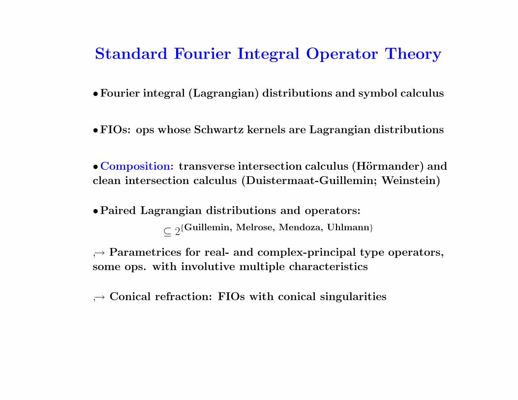
Standard Fourier Integral Operator Theory

•Fourier integral (Lagrangian) distributions and symbol calculus

•FIOs: ops whose Schwartz kernels are Lagrangian distributions

•Composition: transverse intersection calculus (Hormander) and

clean intersection calculus (Duistermaat-Guillemin; Weinstein)

•Paired Lagrangian distributions and operators:

⊆ 2{Guillemin, Melrose, Mendoza, Uhlmann}

↪→ Parametrices for real- and complex-principal type operators,

some ops. with involutive multiple characteristics

↪→ Conical refraction: FIOs with conical singularities

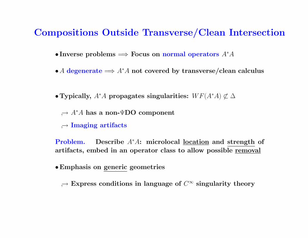
Compositions Outside Transverse/Clean Intersection

• Inverse problems =⇒ Focus on normal operators A∗A

•A degenerate =⇒ A∗A not covered by transverse/clean calculus

•Typically, A∗A propagates singularities: WF (A∗A) 6⊂ ∆

↪→ A∗A has a non-ΨDO component

↪→ Imaging artifacts

Problem. Describe A∗A: microlocal location and strength of

artifacts, embed in an operator class to allow possible removal

•Emphasis on generic geometries

↪→ Express conditions in language of C∞ singularity theory

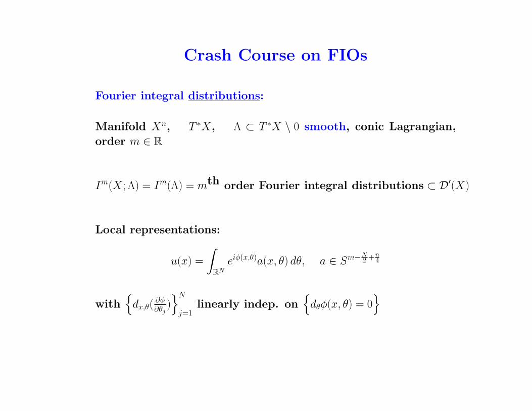
Crash Course on FIOs

Fourier integral distributions:

Manifold Xn, T ∗X, Λ ⊂ T ∗X \ 0 smooth, conic Lagrangian,

order m ∈ R

Im(X ; Λ) = Im(Λ) = mth order Fourier integral distributions ⊂ D′(X)

Local representations:

u(x) =

∫RNeiφ(x,θ)a(x, θ) dθ, a ∈ Sm−

N2 +n

4

with{dx,θ(

∂φ∂θj

)}Nj=1

linearly indep. on{dθφ(x, θ) = 0

}

Fourier integral operators:

X × Y , C ⊂ (T ∗X \ 0)× (T ∗Y \ 0) a canonical relation

Im(C) = Im(X, Y ;C) = {A : D(Y ) −→ E(Y ) |KA ∈ Im(X × Y ;C ′)}

• Inherits symbol calculus from Im(C ′)

•X = Y, C = ∆T ∗Y =⇒ Im(∆T ∗Y ) = Ψm(Y )

•Compositions. Transverse/clean intersection calculus: if

(C1 × C2) ∩ (T ∗X ×∆T ∗Y × T ∗Z) cleanly with excess e ∈ Z+

then C1 ◦ C2 ⊂ T ∗X × T ∗Z is a smooth canonical relation and

A ∈ Im1(X, Y ;C1), B ∈ Im2(Y, Z;C2) =⇒ AB ∈ Im1+m2+e2(X,Z;C1 ◦ C2)

Nondegenerate FIOs

Suppose dimX = nX ≥ dimY = nY , C ⊂ (T ∗X \ 0)× (T ∗Y \ 0)

C ↪→ T ∗X × T ∗YπL↙

πR↘

T ∗X T ∗Y

Projections: πL : C −→ T ∗X, πR : C −→ T ∗Y

Note: dimT ∗Y = 2nY ≤ dimC = nX + nY ≤ dimT ∗X = 2nX

Def. Say that C is a nondegenerate canonical relation if

(*) πR a submersion ⇐⇒ πL an immersion

C nondegenerate =⇒ Ct ◦ C covered by clean intersection

calculus, with excess e = nX − nY

If strengthen (*) to

(**) πL is an injective immersion,

then Ct ◦ C ⊂ ∆T ∗Y and

A ∈ Im1−e4(C), B ∈ Im2−e4(C) =⇒ A∗B ∈ Im1+m2(∆T ∗Y ) = Ψm1+m2(Y )

• Integral geometry: For a generalized Radon transform

R : D(Y ) −→ E(X), (**) is the Bolker condition of Guillemin,

R∗R ∈ Ψ(Y ) =⇒ parametrices and local injectivity

• Seismology: For the linearized scattering map F , under var-

ious acquisition geometries, (**) is the traveltime injectivity

condition (Beylkin, Rakesh, ten Kroode-Smit-Verdel, Nolan-

Symes),

F ∗F ∈ Ψ(Y ) =⇒ singularities of sound speed

are determined by singularities of pressure measurements

———————

Q: What happens if Bolker/T.I.C. are violated?

A: Artifacts

Problem. (1) Describe structure and strength of the artifacts

(2) Remove (if possible)

Q. A general theory of FIOs?

In general, if C ⊂ T ∗X × T ∗Y , A ∈ Im1(C), B ∈ Im2(C), then

WF (KA∗B) ⊆ Ct ◦ C ⊂ T ∗Y × T ∗Y

is some kind of Lagrangian variety, containing points in ∆T ∗Y ,

but other points as well.

A general theory of FIOs would have to:

(1) describe such Lagrangian varieties,

(2) associate classes of Fourier integral-like distributions,

(3) describe the composition of operators whose Schwartz

kernels are such, and

(4) give L2 Sobolev estimates for these.

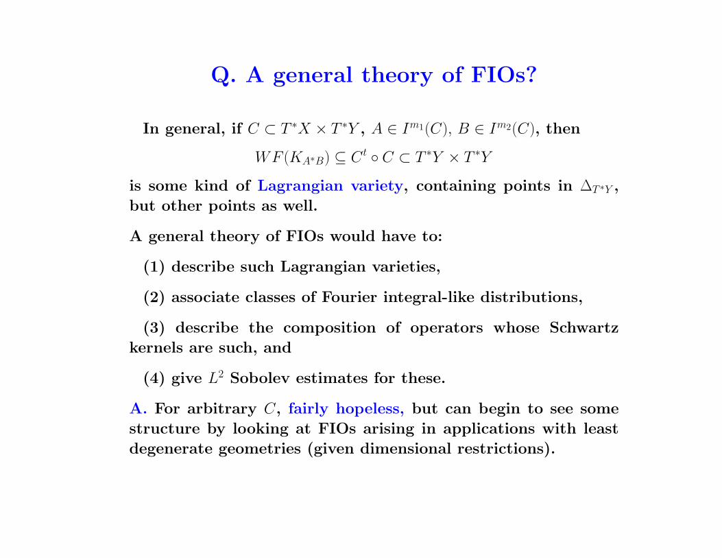
Q. A general theory of FIOs?

In general, if C ⊂ T ∗X × T ∗Y , A ∈ Im1(C), B ∈ Im2(C), then

WF (KA∗B) ⊆ Ct ◦ C ⊂ T ∗Y × T ∗Y

is some kind of Lagrangian variety, containing points in ∆T ∗Y ,

but other points as well.

A general theory of FIOs would have to:

(1) describe such Lagrangian varieties,

(2) associate classes of Fourier integral-like distributions,

(3) describe the composition of operators whose Schwartz

kernels are such, and

(4) give L2 Sobolev estimates for these.

A. For arbitrary C, fairly hopeless, but can begin to see some

structure by looking at FIOs arising in applications with least

degenerate geometries (given dimensional restrictions).

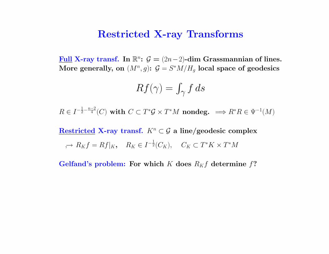
Restricted X-ray Transforms

Full X-ray transf. In Rn: G = (2n−2)-dim Grassmannian of lines.

More generally, on (Mn, g): G = S∗M/Hg local space of geodesics

Rf (γ) =∫γ f ds

R ∈ I−12−

n−24 (C) with C ⊂ T ∗G × T ∗M nondeg. =⇒ R∗R ∈ Ψ−1(M)

Restricted X-ray transf. Kn ⊂ G a line/geodesic complex

↪→ RKf = Rf |K, RK ∈ I−12(CK), CK ⊂ T ∗K × T ∗M

Gelfand’s problem: For which K does RKf determine f?

G. - Uhlmann: K well-curved =⇒ πR : CK −→ T ∗M is a fold

Gelfand cone condition =⇒ πL : CK −→ T ∗G is a blow-down

Form general class of canonical relations C ⊂ T ∗X × T ∗Y with

this blowdown-fold structure, cf. Guillemin; Melrose.

Ct ◦ C not covered by clean intersection calculus

Theorem. (i) Ct ◦ C ⊂ ∆T ∗Y ∪ C, with C the (smooth) flowout

generated by the image in T ∗Y of the fold points of C.

Furthermore, ∆ ∩ C cleanly in codimension 1.

(ii) A ∈ Im1(C), B ∈ Im2(C) =⇒ A∗B ∈ Im1+m2,0(∆, C) (paired

Lagrangian class of Melrose-Uhlmann-Guillemin)

————————

A union of two cleanly intersecting canonical relations, such as

∆ ∪ C, should be thought of as a Lagrangian variety.

Inverse problem of exploration seismology

• Earth = Y = R3+ = {y3 > 0}, c(y) = unknown sound speed

↪→ �c =1

c(y)2∂2t −∆y on Y × R

Problem: Determine c(y) from seismic experiments

• Fix source s ∈ ∂Y ∼ R2 and solve

�cp(y, t) = δ(y − s)δ(t), p ≡ 0 for t < 0

• Record pressure (solution) at receivers r ∈ ∂Y, 0 < t < T

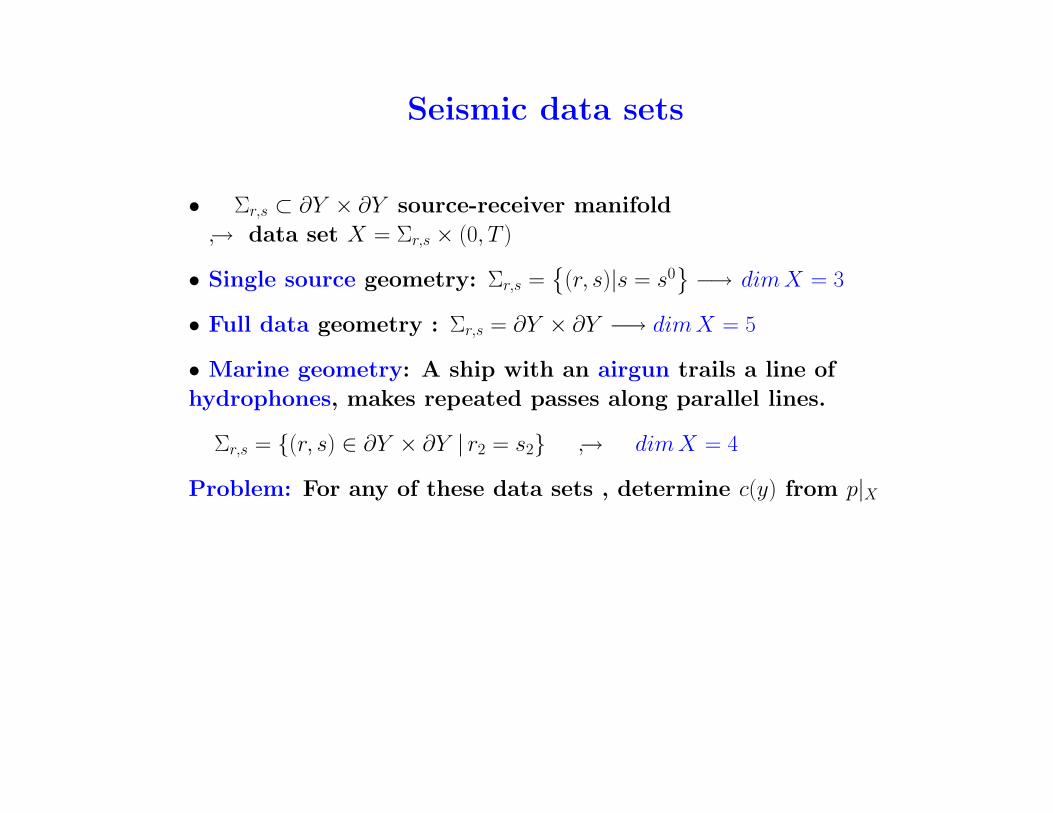
Seismic data sets

• Σr,s ⊂ ∂Y × ∂Y source-receiver manifold

↪→ data set X = Σr,s × (0, T )

• Single source geometry: Σr,s ={

(r, s)|s = s0}−→ dimX = 3

• Full data geometry : Σr,s = ∂Y × ∂Y −→ dimX = 5

• Marine geometry: A ship with an airgun trails a line of

hydrophones, makes repeated passes along parallel lines.

Σr,s = {(r, s) ∈ ∂Y × ∂Y | r2 = s2} ↪→ dimX = 4

Problem: For any of these data sets , determine c(y) from p|X

Linearized Problem

• Assume c(y) = c0(y) + (δc) (y), background c0 smooth and known

• δc small, singular, unknown ↪→ p ∼ p0 + δp

where p0 = Green’s function for �c0

Goal: (1) Determine δc from δp|X, or at least

(2) Singularities of δc from singularities of δp|X

High frequency linearized seismic inversion

Microlocal analysis

δp induced by δc satisfies

�c0(δp) =2

(c0)3· ∂

2p0

∂t2· δc, δp ≡ 0, t < 0,

Linearized scattering operator F : δc −→ δp|X

• For single source, no caustics for background c0(y) =⇒

F ∈ I1(C), C a local canonical graph, F ∗F ∈ Ψ2(Y ) (Beylkin)

• Mild assumptions =⇒ F is an FIO (Rakesh)

Traveltime Injectivity Condition =⇒ F ∈ Im(C), C nondeg.

=⇒ F ∗F ∈ Ψ(Y ) (ten Kroode - Smit -Verdel; Nolan - Symes)

• TIC can be weakened to just: πL an immersion, and then

F ∗F = ΨDO + smoother FIOs (Stolk)

But: TIC unrealistic - need to deal with caustics.

• Low velocity lens =⇒ F ∗F doesn’t satisfy expected estimates

and can’t be a ΨDO (Nolan–Symes)

• Problem. Study F for different data sets and for backgrounds

with generic and nonremovable caustics (conjugate points,

multipathing): folds, cusps, swallowtails, ...

(1) What is the structure of C?

(2) What can one say about F ∗F? Where are the artifacts and

how strong are they?

(3) Can F ∗F be embedded in a calculus?

(4) Can the artifacts be removed?

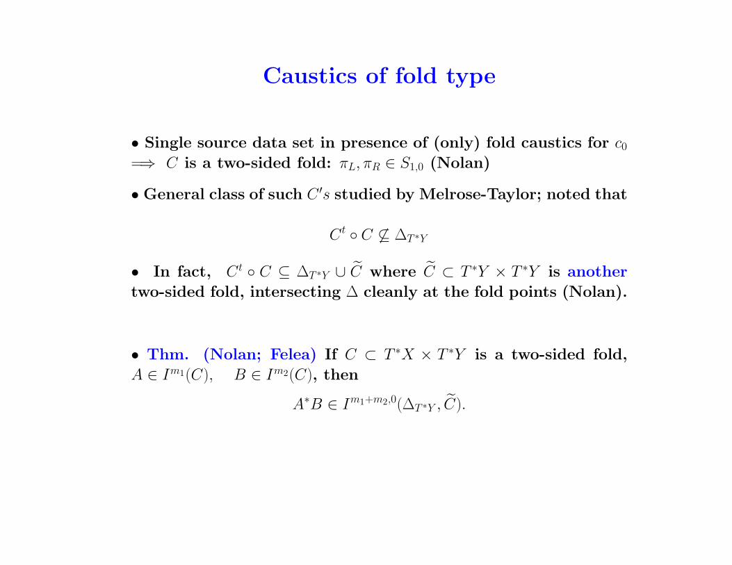
Caustics of fold type

• Single source data set in presence of (only) fold caustics for c0

=⇒ C is a two-sided fold: πL, πR ∈ S1,0 (Nolan)

• General class of such C ′s studied by Melrose-Taylor; noted that

Ct ◦ C 6⊆ ∆T ∗Y

• In fact, Ct ◦ C ⊆ ∆T ∗Y ∪ C where C ⊂ T ∗Y × T ∗Y is another

two-sided fold, intersecting ∆ cleanly at the fold points (Nolan).

• Thm. (Nolan; Felea) If C ⊂ T ∗X × T ∗Y is a two-sided fold,

A ∈ Im1(C), B ∈ Im2(C), then

A∗B ∈ Im1+m2,0(∆T ∗Y , C).

• For 3D linearized single source seismic problem, the presence

of fold caustics thus results in strong, nonremovable artifacts:

F ∗F ∈ I2,0(∆, C) ↪→ I2(∆ \ C) + I2(C \∆)

Caustics of fold type - Marine data set

(Felea-G.) Now use 4-dim. marine data set X, and suitable

interpretation of fold caustics. Then:

• For C ⊂ T ∗X × T ∗Y , πR : C −→ T ∗Y is a submersion with folds

and πL : C −→ T ∗X is a cross-cap (or Whitney/Cayley umbrella)

• Define a general class of folded cross-cap canonical relations

C2n+1 ⊂ T ∗Xn+1 × T ∗Y n

• For these Ct ◦ C ⊆ ∆T ∗Y ∪ C where C ⊂ T ∗Y × T ∗Y is another

two-sided fold, intersecting ∆ cleanly at the fold points.

• If A ∈ Im1(C), B ∈ Im2(C), then A∗B ∈ Im1+m2−12 ,

12(∆T ∗Y , C)

• N.B. Need to establish, work with a weak normal form for C.

• For the seismology problem,

F ∗F ∈ I32 ,

12(∆, C) ↪→ I2(∆ \ C) + I

32(C \∆)

• The artifact is formally 1/2 order smoother,

but actually removing it seems to be very challenging!

Problem. Develop an effective functional calculus for Ip,l(∆, C).

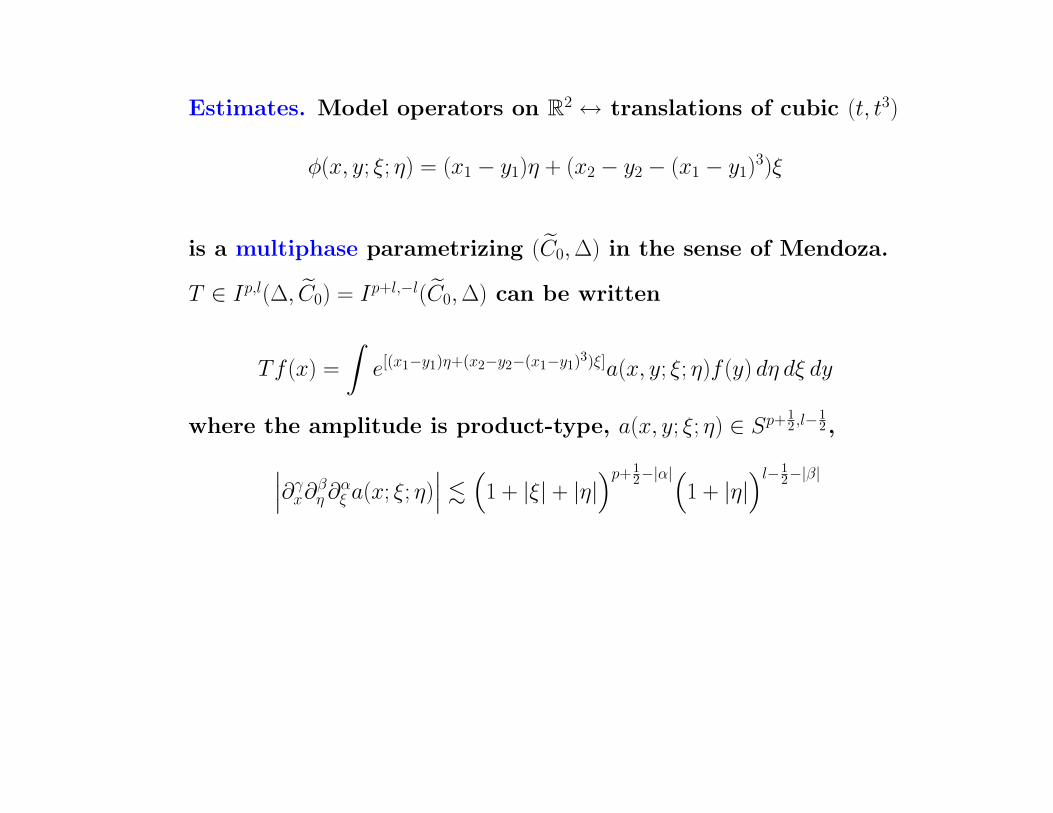
Estimates. Model operators on R2 ↔ translations of cubic (t, t3)

φ(x, y; ξ; η) = (x1 − y1)η + (x2 − y2 − (x1 − y1)3)ξ

is a multiphase parametrizing (C0,∆) in the sense of Mendoza.

T ∈ Ip,l(∆, C0) = Ip+l,−l(C0,∆) can be written

Tf (x) =

∫e[(x1−y1)η+(x2−y2−(x1−y1)3)ξ]a(x, y; ξ; η)f (y) dη dξ dy

where the amplitude is product-type, a(x, y; ξ; η) ∈ Sp+12 ,l−

12 ,∣∣∣∂γx∂βη ∂αξ a(x; ξ; η)

∣∣∣ . (1 + |ξ| + |η|)p+1

2−|α|(1 + |η|

)l−12−|β|

Thm. (Felea-G.-Pramanik) If T ∈ Ip,l(∆, C), C = C0, Css or Cmar,

then T : Hs −→ Hs−r for

r = p +1

6, l < −1

2

= p + 1/6 + ε, l = −1

2, ∀ε > 0

= p + (l + 1)/3, −1

2< l <

1

2

= p + l, l ≥ 1

2.

Idea of proof: Combine parabolic cutoff with Phong-Stein-Cuccagna

decomposition. Pick 13 ≤ δ ≤ 1

2. Localize to |ξ| ∼ 2j, |η| ∼ 2k:

T = T0 +

∞∑j=0

j∑k=δj

Tjk + T∞

where T0 ∈ Imδ(C), T∞ ∈ Ip+l(∆) and Tjk can be shown to satisfy

almost orthogonality. Optimize over δ.

Caustics of cusp type

(G.-Felea) Single source geometry, but now assume that rays

from source form a cusp caustic in Y . The F ∈ I1(C) with C

having the following structure.

Def. If X and Y are manifolds of dimension n ≥ 3, then a canon-

ical relation C ⊂ (T ∗X \ 0) × (T ∗Y \ 0) is a flat two-sided cusp if

(i) both πL : C −→ T ∗X and πR : C −→ T ∗Y have at most cusp

singularities;

(ii) the left- and right-cusp points are equal:

Σ1,1(πL) = Σ1,1(πR) := Σ1,1; and

(iii) πL(Σ1,1) ⊂ T ∗X and πR(Σ1,1) ⊂ T ∗Y are coisotropic (involutive)

nonradial submanifolds.

Model operators. Translations of cubic (t, t2, t4) in R3 ↪→

A ∈ Im(Cmod) can be written

Af (x) =

∫R2eiφmod(x,y,θ)a(x, y, θ)f (y)dθ, a ∈ S0

φmod(x, y, θ) =(x2 − y2 − (x1 − y1)2)

)θ2 +

(x3 − y3 − (x1 − y1)4

)θ3

For A ∈ Im(Cmod),

KA∗A(x, y) =

∫R3eiφ a dθ2 dθ3 dτ with

φ = (x2− y2 +τ

θ3(x1− y1))θ2 + (x3− y3 +

1

2(x1− y1)(

τ

θ3)3 +

1

2

τ

θ3(x1− y1)3)θ3

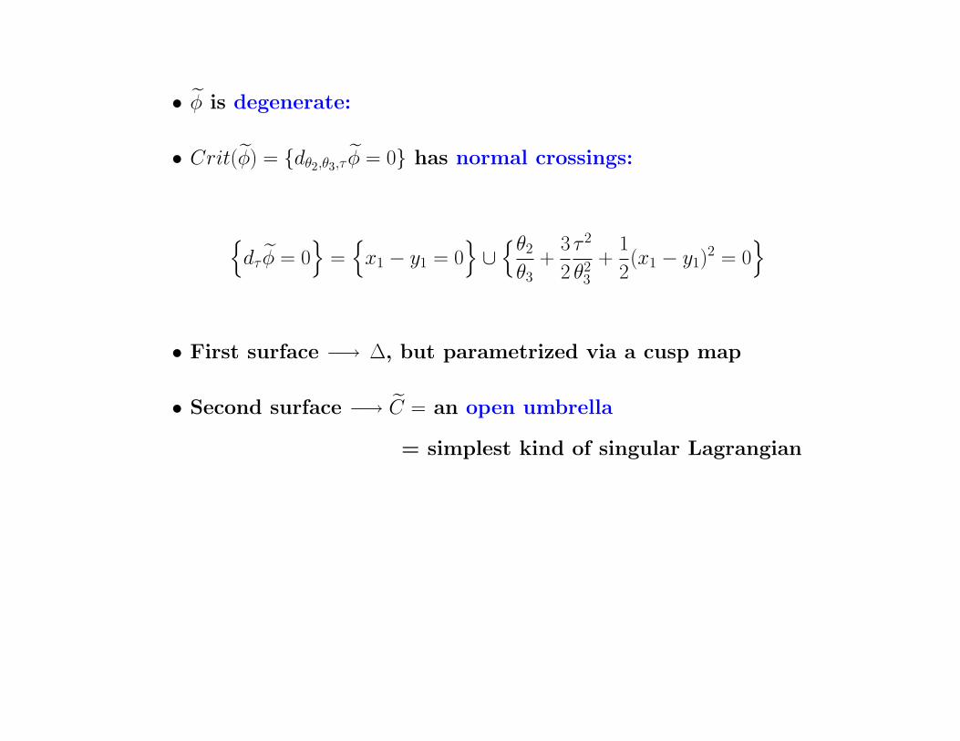
• φ is degenerate:

• Crit(φ) = {dθ2,θ3,τ φ = 0} has normal crossings:

{dτ φ = 0

}={x1 − y1 = 0

}∪{θ2

θ3+

3

2

τ 2

θ23

+1

2(x1 − y1)2 = 0

}

• First surface −→ ∆, but parametrized via a cusp map

• Second surface −→ C = an open umbrella

= simplest kind of singular Lagrangian

Open umbrellas

• Closed umbrella (Whitney-Cayley, crosscap) f : R2 −→ R3

f (x, y) = (x2, y, xy) = (u, v, w) with image {w2 = uv2}

• Immersion away from origin, rank(df (0)) = 1

Embedding off of {y = 0}, where 2-1

• Lift to Lagrangian map g : R2 −→ (R4, ω), ω = dξ1 ∧ dx1 + dξ2 ∧ dx2

g(x, y) = (x2, y;xy, 23x

3) = (x1, x2; ξ1, ξ2)

• Image is a smooth Lagrangian ( g∗ω = 0) away from the non-

removable isolated singularity at origin (Givental)

• General Λn ⊂ (M 2n, ω), umbrella tip Σ1 is codim 2

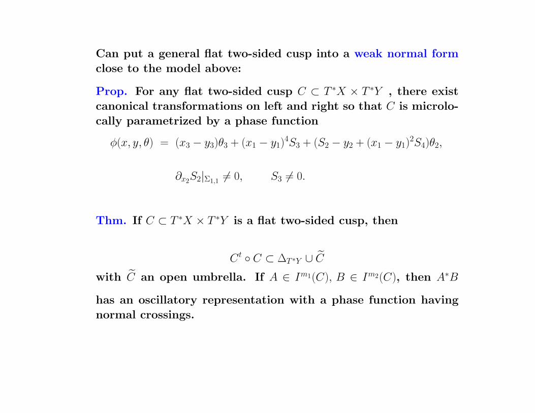
Can put a general flat two-sided cusp into a weak normal form

close to the model above:

Prop. For any flat two-sided cusp C ⊂ T ∗X × T ∗Y , there exist

canonical transformations on left and right so that C is microlo-

cally parametrized by a phase function

φ(x, y, θ) = (x3 − y3)θ3 + (x1 − y1)4S3 + (S2 − y2 + (x1 − y1)2S4)θ2,

∂x2S2|Σ1,1 6= 0, S3 6= 0.

Thm. If C ⊂ T ∗X × T ∗Y is a flat two-sided cusp, then

Ct ◦ C ⊂ ∆T ∗Y ∪ Cwith C an open umbrella. If A ∈ Im1(C), B ∈ Im2(C), then A∗B

has an oscillatory representation with a phase function having

normal crossings.

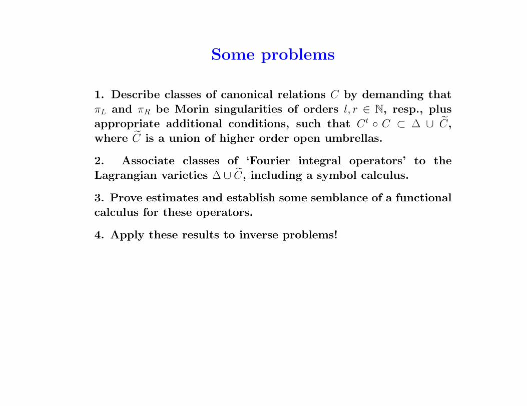
Some problems

1. Describe classes of canonical relations C by demanding that

πL and πR be Morin singularities of orders l, r ∈ N, resp., plus

appropriate additional conditions, such that Ct ◦ C ⊂ ∆ ∪ C,

where C is a union of higher order open umbrellas.

2. Associate classes of ‘Fourier integral operators’ to the

Lagrangian varieties ∆ ∪ C, including a symbol calculus.

3. Prove estimates and establish some semblance of a functional

calculus for these operators.

4. Apply these results to inverse problems!

Thank you, and

Happy Birthday, Gunther !