Can the Dynamics of Petroleum Futures be Forecasted? Evidence from Major Markets

Thalia Chantziara1 & George Skiadopoulos2

¹ Independent

² Dept. of Banking and Financial Management, University of Piraeus &

Financial Options Research Centre, University of Warwick

Commodities 200717 January, 2007 – Birkbeck College

2

Background - Motivation

• Futures on various petroleum products have become very popular.

• The whole term structure of futures prices is of interest.

• The term structure evolves stochastically.

• The trading and hedging of petroleum futures is challenging.

• Can we forecast the daily evolution of the petroleum term structure per se?

3

This paper - Contributions

• What will be the forecasting variables?

• Principal Components Analysis (PCA) is used to this end (Stock & Watson, 2002a, JASA/ 2002b, JBES, Artis et al., 2005, JF). Let the data speak themselves. The PCs subsume all the available information. Spillover effects may also be detected.

• Rich data set of petroleum futures.

4

Related Literature

• PCA & Petroleum Markets.

Cortazar & Schwartz (JoD, 1994), Tolmasky & Hindanov (JFM, 2002).

Clewlow and Strickland (1999).

Järvinen (2003).

• Forecasting the prices of petroleum futures.

Sadorsky (EE, 2002).

Cabbibo & Fiorenzani (Energy Risk, 2004).

5

Outline• Background – Motivation.

• This paper – Contributions – Related Literature.

• The Data.

• Principal Components Analysis (PCA): Results.

• PCA & Forecasting Power.

• Autoregressions.

• Conclusions – Implications – Future research.

6

The Data Set

• Daily settlement futures prices on the: WTI NYMEX Crude oil (CL). IPE Brent Crude Oil (CO). Heating Oil (HO). Gasoline (HU).

• The Bloomberg generic series are used. Filtering constraints. CL1-CL9, CO1-CO7, HO1-HO7, HU1-HU7.

• The sample is chosen over 1/1/1993 – 31/12/2003.

7

Evolution of the WTI Term Structure

-6.00

-3.00

0.00

3.00

6.00

9.00

$/B

arre

l

First minus Second First minus Longest

8

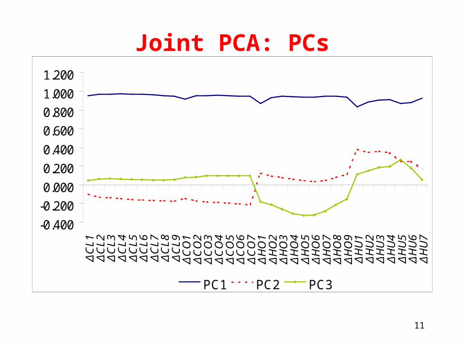
PCA: Results

• Separate PCA & Joint PCA.

• PCA has been applied to the daily changes.

• Three principal components (PCs) are retained.

• Stability of the results has been checked.

9

Percentage of Variance Explained by PCs

NYMEX IPE Heating Oil

Gasoline

Separate PCA

1st 97.21 96.66 93.56 88.11

2nd 99.58 99.23 97.74 95.08

3rd 99.9 99.73 99.31 96.9

4rth 99.96 99.88 99.81 98.18

Joint PCA

1st 87.12

90.79

93.6

95.23

2nd

3rd

4rth

10

NYMEX Crude Oil Futures

-0.400

-0.200

0.000

0.200

0.400

0.600

0.800

1.000

1.200

ΔCL1 ΔCL2 ΔCL3 ΔCL4 ΔCL5 ΔCL6 ΔCL7 ΔCL8 ΔCL9

PC1 PC2 PC3

Gasoline Futures

-0.400

-0.200

0.000

0.200

0.400

0.600

0.800

1.000

1.200

ΔHU1 ΔHU2 ΔHU3 ΔHU4 ΔHU5 ΔHU6 ΔHU7

PC1 PC2 PC3

11

Joint PCA: PCs

-0.400

-0.200

0.000

0.200

0.400

0.600

0.800

1.000

1.200Δ

CL1

ΔC

L2Δ

CL3

ΔC

L4Δ

CL5

ΔC

L6Δ

CL7

ΔC

L8Δ

CL9

ΔC

O1

ΔC

O2

ΔC

O3

ΔC

O4

ΔC

O5

ΔC

O6

ΔC

O7

ΔH

O1

ΔH

O2

ΔH

O3

ΔH

O4

ΔH

O5

ΔH

O6

ΔH

O7

ΔH

O8

ΔH

O9

ΔH

U1

ΔH

U2

ΔH

U3

ΔH

U4

ΔH

U5

ΔH

U6

ΔH

U7

PC1 PC2 PC3

12

PCA and Forecasting Power: Setting

• Let be the j-maturity series measured at time t, j=CL1,…, CL9, CO1,…, CO7, HO1,…, HO9, HU1,…, HU7.

jtF

• Separate PCA:3 3 3 3

, 1 , 1 , 1 , 11 1 1 1

,jt k k t k k t k k t k k t t

k k k k

F c a CLPC b COPC c HOPC d HUPC u j

• Joint PCA:

1 1, 1 2 2, 1 3 3, 1 , .jt t t t tF c a PC a PC a PC u j

• The regressors are stationary, non-normal though.

• General to specific approach is followed.

13

PCA and Forecasting Power: Results

14

Separate PCA: NYMEX Crude Oilc a 1 a 2 a 3 b 1 b 2 b 3 c 1 c 2 c 3 d 1 d 2 d 3

(t -stat)

(t -stat)

(t -stat)

(t -stat)

(t -stat)

(t -stat)

(t -stat)

(t -stat)

(t -stat)

(t -stat)

(t -stat)

(t -stat)

(t -stat)

CL1 - - - - - - - - - - - - - - -- - - - - - - - - - - - - -

CL2 - - - - - - - - - - - - - - -- - - - - - - - - - - - - -

CL3 - - - - - - 0.029 - - - - - - 0.004 6.629- - - - - - (2.2) - - - - - - (0.01)

CL4 - - - - - - 0.026 - - - - - - 0.004 6.285- - - - - - (2.2) - - - - - - (0.01)

CL5 - - - - - - 0.024 - - - - - - 0.004 6.052- - - - - - (2.2) - - - - - - (0.01)

CL6 - - - - - - - - - - - - - - -- - - - - - - - - - - - - -

CL7 - - - - - - - - - - - - - - -- - - - - - - - - - - - - -

CL8 - - - - - - - - - - - - - - -- - - - - - - - - - - - - -

CL9 - - - - - - - - - - - - - - -- - - - - - - - - - - - - -

j R 2 F -stat (prob)

15

Separate PCA: IPE Crude Oil

c a 1 b 1 b 2 b 3 c 1 d 1

(t -stat) (t -stat) (t -stat) (t -stat) (t -stat) (t -stat) (t -stat)CO1 - 0.176 -0.203 - - - - 0.02 13.293

- (3.7) (-3.7) - - - - (0.00)CO2 - 0.145 -0.178 - 0.041 - - 0.03 12.145

- (3.5) (-3.8) - (2.7) - - (0.00)CO3 - 0.143 -0.169 - 0.036 - - 0.03 12.721

- (3.9) (-4.2) - (2.8) - - (0.00)CO4 - 0.133 -0.164 - - - - 0.02 15.666

- (4.1) (-4.6) - - - - (0.00)CO5 - 0.125 -0.162 - - - - 0.03 18.108

- (4.2) (-4.9) - - - - (0.00)CO6 - 0.114 -0.155 - - - - 0.03 18.859

- (4) (-4.8) - - - - (0.00)CO7 - 0.105 -0.149 - - - - 0.03 19.581

- (3.7) (-4.7) - - - - (0.00)

j R 2 F -stat (prob)

16

Separate PCA: Heating Oilc a 1 a 2 a 3 b 1 b 2 b 3 c 1 c 2 c 3 d 1 d 2 d 3

(t -stat)

(t -stat)

(t -stat)

(t -stat)

(t -stat)

(t -stat)

(t -stat)

(t -stat)

(t -stat)

(t -stat)

(t -stat)

(t -stat)

(t -stat)

HO1 - - - - - - 0.091 - - - - - - 0.003 4.796- - - - - - (2.3) - - - - - - (0.03)

HO2 - - - - - - 0.095 - - - - - - 0.005 7.039- - - - - - (2.5) - - - - - - (0.01)

HO3 - - - - - - 0.096 - - - - - - 0.006 8.697- - - - - - (2.8) - - - - - - (0.00)

HO4 - - - - - - 0.088 - - - - - - 0.006 8.563- - - - - - (2.5) - - - - - - (0.00)

HO5 - - - - - - 0.087 - - - - - - 0.006 9.315- - - - - - (2.7) - - - - - - (0.00)

HO6 - - - - - - 0.094 - - - - - - 0.008 11.852- - - - - - (3.0) - - - - - - (0.00)

HO7 - - - - - - 0.086 - - - - - - 0.007 10.821- - - - - - (2.8) - - - - - - (0.00)

HO8 - - - - - - 0.075 - - - - - - 0.006 8.843- - - - - - (2.5) - - - - - - (0.00)

HO9 - - - - - - - - - - -0.084 - 0.008 8.941- - - - - - - - - - - (-3.0) - (0.00)

j R 2 F -stat (prob)

17

Separate PCA: Gasolinec a 1 a 2 a 3 b 1 b 2 b 3 c 1 c 2 c 3 d 1 d 2 d 3

(t -stat)

(t -stat)

(t -stat)

(t -stat)

(t -stat)

(t -stat)

(t -stat)

(t -stat)

(t -stat)

(t -stat)

(t -stat)

(t -stat)

(t -stat)

HU1 - - - - - - - - -0.087 - - - - 0.002 3.817- - - - - - - - (-2.0) - - - - (0.05)

HU2 - - - - - - - - - - - - - - -- - - - - - - - - - - - - -

HU3 - - - - - - - - - - - - - - -- - - - - - - - - - - - - -

HU4 - - - - - - - - - - - - - - -- - - - - - - - - - - - - -

HU5 - - - - - - - - - - - - - - -- - - - - - - - - - - - - -

HU6 - - - - - - 0.083 - - - -0.131 - - 0.021 8.852- - - - - - (2.1) - - - (-2.6) - - (0.00)

HU7 - 0.283 - - - - - - - - -0.353 - - 0.025 14.033- (3.9) - - - - - - - - (-5.1) - - (0.00)

j R 2 F -stat (prob)

18

Joint PCA: Results• The joint PCs have no predictive power in the case of NYMEX & IPE

crude oil. c a 1 a 2 a 3

(t -stat)

(t -stat)

(t -stat)

(t -stat)

HO1 - - - - -- - - -

HO2 - - -0.17 - 0.01- - (-2.4) -

HO3 - - -0.18 - 0.02- - (-2.7) -

HO4 - - -0.18 - 0.02- - (-3.0) -

HO5 - - -0.17 - 0.02- - (-2.9) -

HO6 - - -0.16 - 0.02- - (-2.9) -

HO7 - - -0.15 - 0.02- - (-2.6) -

HO8 - - -0.13 - 0.01- - (-2.5) -

HO9 - - -0.12 - 0.01- - (-2.2) -

HU1 - - - - -- - - -

HU2 - - - - -- - - -

HU3 - - -0.15 - 0.01- - (-2.3) -

HU4 - - -0.17 - 0.01- - (-2.7) -

HU5 - - -0.17 - 0.01- - (-2.7) -

HU6 - - -0.24 - 0.03- - (-3.8) -

HU7 - - -0.21 - 0.03- - (-3.6) -

Heating Oil

Gasoline

j R 2

19

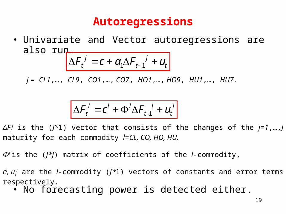
Autoregressions

• Univariate and Vector autoregressions are also run.

1 1j jt t tF c a F u

-1l l l l lt t tF c F u

j = CL1,…, CL9, CO1,…, CO7, HO1,…, HO9, HU1,…, HU7.

ΔFtl is the (J*1) vector that consists of the changes of the j=1,…,J maturity for each

commodity l=CL, CO, HO, HU,

Φl is the (J*J) matrix of coefficients of the l-commodity,

cl, utl are the l-commodity (J*1) vectors of constants and error terms respectively.

• No forecasting power is detected either.

20

Conclusions• Can we forecast the term structure of petroleum futures?

PCA has been used (separately & jointly). A rich data set has been employed.

• Three factors govern the dynamics of the petroleum futures prices.

• Some of the factors are significant but the R2’s are very small.

• Results are corroborated by univariate and vector autoregressions.

21

Implications – Future Research• The dynamics of petroleum futures can not be forecasted.

• The dynamics of petroleum futures prices are stable over time.

• Spillover effects are detected between the four markets (also Lin & Tamvakis, 2001, EE; Girma and Paulson,1999, JFM).

• Future research: Alternative variants of the PCA model may be useful. GARCH-type effects. Non-linear PCA models.

22

Thank you for listening!

gskiado@unipi.gr

http://iweb.xrh.unipi.gr/~gskiado/index.htm