Can Natural Experiments Measure Behavioral Responses...

Can Natural Experiments Measure Behavioral

Responses to Environmental Risks?

JARED C. CARBONE, DANIEL G. HALLSTROMand V. KERRY SMITH*Department of Agricult. and Resource Econ., North Carolina State University, Box 8109,Raleigh, North Carolina, 27695-8109, USA; *Author for correspondence (e-mail: kerry_

[email protected])

Accepted 15 May 2005

Abstract. Efforts to measure people’s responses to spatially delineated risks confront the

potential for correlation between these risks and other, unobserved characteristics of theselocations. The possibility of correlation arises in part because individuals observe otherlocational attributes that can be expected to influence the hedonic equilibrium. One responseto this problem is to use events from nature to exploit both temporal and spatial variation in

the behavioral responses of interest. This paper evaluates the use of hurricanes as a source ofnew risk information to households in coastal counties potentially subject to the effects ofthese storms. We study the extent to which housing prices before and after hurricane Andrew,

a hurricane with unprecedented property loss, reveal how Floridians responded to the riskinformation provided by the storm. Two counties are selected – one without and another withdamage from the hurricane. To evaluate the plausibility of using quasi-random experiments

for locations not directly affected by natural events, we compare Lee County’s results to thoseof Dade County, where the majority of the damage occurred. Our findings suggest, aftercontrolling for ex post storm damage and changes in insurance markets, there is a reasonably

high level of consistency in a repeat sales model’s ability to estimate the effects of the riskinformation conveyed by the storm for both counties.

Key words: hurricane risk, repeat sales, hedonic models

JEL classification: Q51, Q54

* Department of Economics, Williams College, Affiliated Economist, CEnREP, North

Carolina State University and University Distinguished Professor, North Carolina StateUniversity, and Resources for the Future University Fellow, respectively. Senior authorship isnot assigned. Thanks are due to Shelby Gerking and two anonymous reviewers for careful andconstructive comments that substantially improved the paper. Michael Darden and Jaren

Pope provided excellent research assistance and Alex Boutaud and Susan Hinton helped tomake sense out of numerous drafts of this work. Smith’s contribution was partially supportedby the United States Department of Homeland Security through the Center for Risk and

Economic Analysis of Terrorism Events (CREATE), grant number EMW-2004-GR-0112.However, any opinion, findings, and conclusions or recommendations in this document arethose of the author(s) and do not necessarily reflect views of the U.S. Department of

Homeland Security.

Environmental & Resource Economics (2006) 33: 273–297 � Springer 2006DOI 10.1007/s10640-005-3610-4

1. Introduction

An ideal test of any factor hypothesized to influence behavior would ran-domly vary it among a sample of the people who are expected to respond.Economic tests rarely meet this standard. As a rule, we must be satisfied withquasi-random experiments, where control is not guaranteed to meet thestandards of a completely random assignment. Often, these experiments arisefrom natural events or exogenous changes that provide clear-cut sources ofvariation in the effect of interest. As Meyer (1995) observes, the careful logicdeveloped as part of these quasi-experiments usually documents why thevariation in a treatment can be considered to be exogenous. It emphasizes theimportance of understanding how measured effects are identified. Recent usesof this logic in environmental economics have relied on differences due topolicy decisions (Chay and Greenstone 2005), variations in aggregate eco-nomic conditions (Chay and Greenstone 2003), and natural events (see Beronet al. 1997 for the case of earthquakes). In each case the unanticipated changeserves to designate who receives a variation in the treatment. As a result, it isargued that the analyst can be reasonably confident assuming the effectexperienced was not the result of a separate behavioral choice that is relatedto the tradeoff estimates (or the tests) derived from the analysis.

When these analyses involve economic outcomes such as housing valuesand treatments that arise from differences in non-market environmentalamenities, two assumptions are important to the chain of logic that assuresthe experiment isolates the effect being measured. The first concerns thehypothesis that is usually of direct interest. People are assumed to recognizethe ‘‘amount’’ of the amenity and respond to it. Second, the analysis requiressome phenomenon to provide a consistent and recognizable variation in theamenity (or disamenity) of interest.

This paper summarizes the finding of an ongoing research program onhurricanes as a source of risk information to coastal residents.1 Our objectivehere is to describe how this second assumption can be important. In our casethe exogenous source of variation in information is a hurricane. Before ithappens, people who live or wish to live along the coast have one set of riskbeliefs. After, they have another. Our question is simple – what is the spatialextent of the new information provided by a large storm? Do we assume it islimited to the area directly affected by the hurricane or does it extend beyondthese locations?

To investigate these questions we use the largest hurricane (in terms ofinsurance industry losses) in U.S. history, Hurricane Andrew. We considertwo counties in Florida: the one that was hit (Dade County) and experiencedabout 20 billion 2004 dollars in insured losses, and a second where the countywas close to the hurricane’s landfall path in Florida (Lee County) but farenough that residents did not experience structural damage.2 We use a repeat

JARED C. CARBONE ET AL.274

sales model for each county separately as well as the spatial location ofprivate homes that sold twice between 1983 and 2000. Our test considerswhether the new risk information we attribute to Andrew influenced thechange in housing prices for those sales that bracket Andrew and were inflood hazard zones versus those that did not satisfy both conditions. Acomparison of separate models for each county provides a plausibility checkon our research strategy. While each analysis faces specialized considerations,a comparison of our estimates of the effects of the hurricane, as new infor-mation, after these added controls are taken into account, provides onemeans to confirm the general logic.

In contrast to many other sources of environmental risk, insurance isavailable for the property losses due to a number of natural hazards,including flood and hurricane damage. Our analysis of the effects of riskinformation controls for the effects of changes in insurance terms. Finally, inthe case of Dade County, to assure we can separate the effects of damagefrom new information, a unique database is used to control for the effects ofstorm damage. That is, homes damaged by the storm may have includedmodernization and structural upgrades in the repairs. Thus, price differencesmeasured for sales that bracket the storm reflect both the effects of riskinformation and any structural changes arising from how repairs wereundertaken.

The analyses in both counties confirm that Andrew appears to havealtered households’ perceptions of the risks of living in coastal locations. Theestimated effect of Andrew is remarkably consistent for the two counties,ranging from about 20 to 30 percent reduction in the pace of increase ofhousing prices for the highest flood risk locations. Efforts to control for theeffects of insurance have a large impact on the estimated effect of the riskinformation in Dade County, but not in Lee County.

Section 2 outlines a simple expected utility model for describing how riskpreferences can be deduced from a hedonic price function. Section 3 reviewsthe basic framework for our natural experiment and describes how it isimplemented in a repeat sales hedonic model. Section 4 discusses our dataand Section 5 summarizes the findings. We conclude with some discussion ofthe implications of our overall research program.

2. Behavioral Responses to Risk

Economic models of behavioral risk adjustments hypothesize that peoplehave incentives to respond to risks they know about. The nature of theirresponse will depend on the costs and benefits of averting the source of therisk or mitigating its potential impact. If these behaviors influence housingprices, then the analyst may have sufficient information to measure howpeople tradeoff money for risk.

CAN NATURAL EXPERIMENTS MEASURE BEHAVIORAL RESPONSES 275

The hedonic property value model is one of the earliest economicframeworks to offer a way to include location with its summary of behav-ioral choices among different types of houses. Early discussions of the modelsought to describe the price function as a reduced form relationship for amatching equilibrium. A key concern has been the ability to recover mea-sures for individual tradeoffs among attributes from the derivatives ofhedonic price equations (see Rosen (1974) and Ekeland et al. (2004)). Whenthe attributes associated with a house are ‘‘attached’’ because of its location,there may be other reasons for questioning our ability to estimate theireffects on price without bias. Rosenzweig and Wolpin’s (2000) review makesthe problem’s source clear. Suppose property values, R, are related to therisk, p, of an undesirable outcome. This risk is conveyed by the location ofeach home. The hedonic price function assumes the relationship betweenprices and spatially differentiated risks is the result of an equilibriummatching of buyers and sellers. The risk is likely to be correlated withimportant, but unknown, sources of variation in the attributes of theproperty as well as the characteristics of both the buyers and the sellers.Attitudes towards risk, differences in households’ ability to respond to risk,and variation in their knowledge are all good candidates for the source ofthis unobserved heterogeneity.3 As a result, ordinary least squares (OLS)estimates of this equilibrium relationship may not provide unbiased mea-sures of the marginal value of a risk reduction to each participant in amatched exchange.4

It is also reasonable to expect in some cases that the locations which areassociated with higher risk may have other desirable attributes. Forexample, homes on or near the ocean have improved access for recreation,can have better views of ocean vistas, and may even have better airquality. Risks of storm damage and flooding are higher for these locationsas well. When there are opposite effects correlated with distance to thecoast, additional information is required to recover an estimate of theeffect of risk. Of course, it is important to recognize that the interpretationof the estimated marginal effect depends in part on the identifying infor-mation.

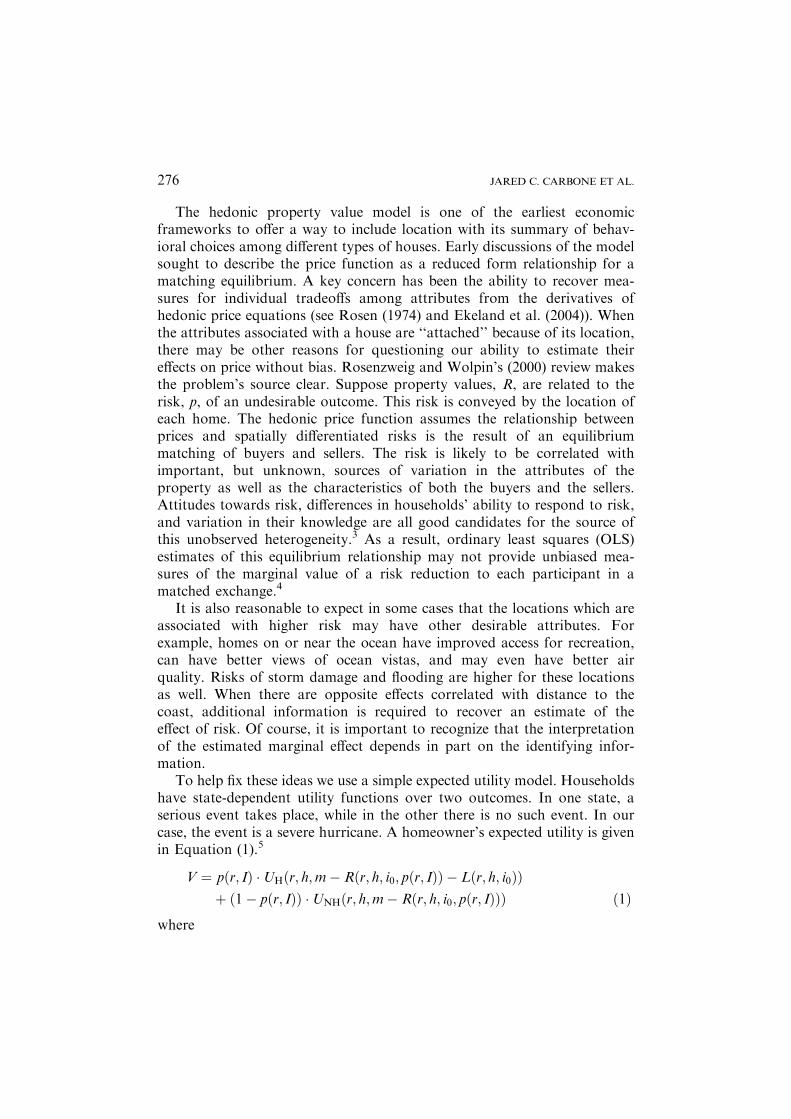
To help fix these ideas we use a simple expected utility model. Householdshave state-dependent utility functions over two outcomes. In one state, aserious event takes place, while in the other there is no such event. In ourcase, the event is a severe hurricane. A homeowner’s expected utility is givenin Equation (1).5

V ¼ pðr; IÞ �UHðr; h;m� Rðr; h; i0; pðr; IÞÞ � Lðr; h; i0ÞÞþ ð1� pðr; IÞÞ �UNHðr; h;m� Rðr; h; i0; pðr; IÞÞÞ ð1Þ

where


m=income (or wealth) less any hazard insurance expectationsh=housing characteristicsr=site attributes that can relate to both the risk of storm hazards and coastal

amenities (e.g. on the coast or a canal)R(.)=hedonic price function (measured in annual terms if m is annual

income)i0=insurance rate per dollar of coverageL(.)=monetary loss due to stormp(r,I)=household’s subjective probability of hurricanes at a given location

and with specific information set (I)Uj (.) = utility for state j, j = H and NH

H labels the utility realized with a case of a hurricane and NH no storm. Boththe level of utility and the marginal utility of income may change with thestate. We assume that households maximize expected utility by selecting r andh conditional on the information (I), insurance rates (i0), and their income.

Assuming an equilibrium that matches buyers and sellers with each fullyinformed, the marginal price of the attribute r is:

Rr ¼pUHr þ ð1� pÞUNHr

pUHm þ ð1� pÞUNHm� pUHm � Lr

pUHm þ ð1� pÞUNHm

þ prðUH �UNHÞpUHm þ ð1� pÞUNHm

ð2Þ

where UHi indicates partial derivative of UH with respect to i. This equationillustrates part of the difficulty with interpreting marginal prices (Rr) withrespect to locational influences (r) on risk. If we interpret r as a locationalattribute, such as distance to the coast, then we would expect that changes inr would lead to a change in hurricane risk. However, the behavioral inter-pretation for this partial derivative is more complex. It can reflect a com-posite of any risk changes along with any other contributions that coastalamenities make to individual well-being aside from risk (the first term). Theremay also be aspects of a location that contribute to losses from a storm (thesecond term). Moreover, in this simple interpretation we are implicitlyassuming that the ‘‘correct’’ equilibrium hedonic price function is known.

To meet our overall objectives, we would like to recover an estimate of Rp,the ex ante incremental option price for a risk change. As noted, spatialdifferences in prices in relation to a measure of distance from the coast areunlikely to provide a reliable basis for gauging behavioral response to risk.Hurricanes as a source of new risk information offer an opportunity to usethe logic of natural experiments to measure RI = RpÆ pI.

Combining temporal variation in risk perceptions with spatial variation inrisk characteristics can also help in avoiding the endogeneity problemsdiscussed earlier. Suppose an exogenous event occurs that provides new


information about a location’s risk. In equilibrium, the marginal impact ofthat new information on the hedonic price is:

RI ¼pI � ðUH �UNHÞ

pUHm þ ð1� pÞUNHmð3Þ

Dividing both sides of Equation (3) by pI provides RI/pI. This relationshipmeasures the incremental option price an individual would be willing to payas an ex ante premium for a home that is located so as to reduce the risk ofdamage and disruption from severe coastal storms. This incremental value isrevealed through the response of housing values to information. It alsorequires an external estimate for how p changes with new information. Hence,a composite of spatial attributes and changes in information about risk (usingthe framework in Equation (3)), along with a measure of pI offer the elementsneeded to measure the ex ante incremental value of risk reductions.

In the context of severe hurricanes it is important to acknowledge thatinsurance terms may also change.6 Thus, the effect we describe in Equation (3)as exclusively associated with information may also lead to changes in i0. Inthis case, the measurement of the incremental option price for a risk changewould require taking into account these insurance related effects as separateinfluences on price. In simple terms, if i0 also responds to I and we ignorechanges in insurance coverage, then Equation (4) would replace (3) as thedescription of the information effect. This process assumes that the appro-priate interpretation of the housing price change is a response to both thestorm as information and as a stimulus for adjustment in the insurancemarket.

RI ¼pI � ðUH �UNHÞ

pUHm þ ð1� pÞUNHm� pUHmLi0 i0IpUHm þ ð1� pÞUNHm

� Ri0 i0I ð4Þ

In the absence of considerable background on the insurance market, thebest we can hope for is to ‘‘take account’’ of the last two terms on the right sideof Equation (4) as a composite but not necessarily tomeasure them separately.7

We hypothesize that residents of a coastal community will learn andupdate their risk perceptions from hurricanes as ‘‘new’’ events. This prospectis especially relevant to situations when there has been a recent history of fewstorms.8 Nonetheless, this proposal has several important qualifications. Thefirst requires that we use the storm to isolate new information about risk ofthese extreme weather events. This treatment cannot be confounded with thedamage due to the actual storm. This concern is one of the issues motivatingthe comparison in this paper. In the first of our efforts in this area, Hallstromand Smith (2005), we selected a ‘‘near miss’’ – a housing market with pre-existing, known risk of hurricanes that was close to, but not hit by, a severestorm. This strategy seeks to avoid the effects of storm related damages onthe models for property values. It implicitly maintains that the selection of a


location generally at risk of storm damage, but that has not been ‘‘hit’’,serves to identify a group of individuals who should be aware of the possi-bility of hurricanes. They may not, depending on past history in relation totheir location choices, have accurate perceptions of the probabilities ofstorms. Under these circumstances, a storm that is ‘‘noticed’’ but that doesnot directly affect them provides new information.

To play this role, Hallstrom and Smith select hurricane Andrew, theglobal insurance industry’s natural event of record, and the responses ofhousing prices in the Special Flood Hazard Areas (SFHA) for Lee County,Florida. In the 20 years prior to August 1992 (when Andrew made landfall)no major hurricanes had passed within 150 miles of Lee County. Andrewmade landfall in Dade County and progressed westward toward the GulfCoast. At its closest point, the hurricane was 75 miles south of Fort Myers.This proximity (along with the assurance that no physical damage occurredin the area) is what Hallstrom and Smith use to characterize the county as a‘‘near miss’’.

This strategy, of course, is simply one ‘‘informational story’’. There areother possibilities, each with important implications for the design of publicdisaster policy. For example, an alternative hypothesis is that markets havealready perfectly capitalized risk characteristics into property prices. In thiscase, the occurrence of a near miss storm is simply a realization from aknown probability distribution with no actual effects. The storm conveys nonew information for the residential housing market. Under these conditionsthere would be no change in the equilibrium prices. In addition, locationspecific characteristics such as past hurricane history and extent of the coastalhazard area might be expected to affect how much new information a seriousstorm conveys. It seems reasonable to ask how we might test the ‘‘near miss’’strategy.

There is no decisive test. As noted at the outset, we propose to evaluate itby considering what happened to housing prices in the county that wasdirectly hit by Andrew. This alternative analysis of the storm’s informationadds a new consideration. It must control for the effects of renovations thatmight take place as part of repairing the hurricane’s damage. It does havesome advantages. The spatial risk designations available to homeownersthrough the FEMA flood maps in Dade County use the same basic scale as inLee County. Both areas experienced a relative lull in activity prior to Andrew.Thus, households in each area might have fairly comparable storm risk beliefs.

3. Using Natural Quasi-Experiment for Environmental Applications

To introduce the logic for our model for uncovering the effect of informa-tion on risk preferences, consider a simple regression version of the modelused in difference-in-differences studies.9 Assume there are two dimensions


distinguishing the structure of the quasi-experiment – the group assignment(j) for each entity in the study and the timing (t) of the outcome that isobserved for each entity. Translating the vocabulary used in the quasi-random experiment to our hedonic model, the price (in annualized terms) Rdesignates the outcome we observe for each entity. An entity in our appli-cation will be a house. A group will be a location and the timing will be thedate of the sale in relation to an external natural event – a hurricane. Thesimplest form of a difference-in-differences framework assumes a linearspecification (in parameters) with effects due to the time (a1), the group (a1),the treatment response (e.g. requiring the simultaneous presence of bothtime and group effects) (b), and the observable and unobservable sources ofheterogeneity (z jit for the observable features and ejit for the unobservable).

lnR jit ¼ a0 þ a1dt þ a1d j þ bd j

t þ cz jit þ e j

it ð5ÞIn Equation (5) dt, d

j are dummy variables equal to one if the group or timedesignation is satisfied and zero otherwise. d j

t is the interaction effect of thetwo conditions (i.e. dtÆ d

j).If we assume, as is often the case in hedonic models, that we do not

completely observe all the attributes of a home and its location that con-tribute to its market price, then we will have incomplete knowledge of zjit. Acommon response (see Palmquist (1982) for the first application), and onethat is consistent with the basic logic of quasi-experiments, is to use a repeatsales model and focus the analysis on the change in prices for the same housesover time. To illustrate, suppose there are two sales periods, t and s. If we usethe difference in sales prices for the same homes (ln Rt)ln Rs), then thistransformation is written in Equation (6).

ðlnRjit� lnRj

isÞ¼ a1ðdt�dsÞþbðdjt�dj

sÞþcðz jit� z jisÞþðejit� e jisÞ ð6Þ

b is the estimate of the incremental price paid to acquire the conditionrepresented by the group and time designations. We see from Equation (7)that it assumes the difference in the logs of the annualized prices before (s=0)and after (t=1) the hypothesized outcome causing the new information forthe group of interest (j=1) compared to the baseline group is constant.

b ¼ lnR1

1 � lnR1

0

� �� lnR

0

1 � lnR0

0

� �ð7Þ

For the repeat sales to capture this difference in mean effects, there must beno other change in observable variables (z j

it = z jis), that contribute to

housing price differences and the unobservables represented by the differencein the errors, (e j

it � e jis), should not be correlated with the effect being mea-

sured.Linking estimates of b to individual risk preferences, as envisioned in

Equation (3), requires that we consider the connections between the price


equation and our model. This connection will be somewhat different for ourtwo counties. In the case of Lee County (i.e. the near miss) there was nodamage from the storm, but the information is nonetheless hypothesized toaffect properties in the FEMA flood hazard zones differently from thoseoutside them.

In addition, Andrew led to substantial turmoil throughout the state in theinsurance market. Florida’s overall response to the insurance crisis Andrewcreated involved the development of two state-run property and casualtyunderwriting associations. However, popular descriptions of the program(see Longman (1994)) indicate that property insurance remained under-priced and did not adequately signal the risks posed to structures in coastalareas. Others note that after Andrew, some companies left the market forcoastal properties completely.10 These events imply that the storm/marketinsurance response described in general terms in Equation (4) needs to beconsidered in modeling price changes for both counties.

In the case of Dade County there is the added concern raised by therequirement to control for whether a property was damaged by the hurri-cane. Commercial data sets available for estimating hedonic models usuallydo not include this type of information. We used two strategies for con-trolling for damages. The first relies on a unique database published by theMiami Herald in December 1992. These data correspond to a damageassessment by housing subdivision conducted by the National Oceanic andAtmospheric Administration (NOAA) after the storm. This survey reportsthe percentage of homes in a neighborhood judged to be uninhabitable afterthe storm. The second uses a geo-coded map of the storm’s path and the windmaps prepared by Wakimoto and Black (1994) for Andrew to estimate aband where storm damage was most likely.11 Each of these effects is repre-sented by a series of interaction terms linking an attribute (i.e., in the FEMAflood zone or in a zone with hurricane damage if the analysis is for DadeCounty) with the timing of the housing sales.

To illustrate this point consider the risk and information relationshipwhich is hypothesized to be relevant for both counties. Re-writing Equation(5) we identify a different perceived risk of hurricane damage based onlocation in the FEMA Special Flood Hazard Zones (SFHA). We begin byassuming that only the designation for being in the zone versus outside it isrelevant. In our final model we investigate whether a more detailed resolutionof sub-zones is possible. Equation (8) describes this single destination –perceived risk based on being inside or outside the SFHA.

lnRit¼Xk

ckzkþFiðbtþbptþgiþ eitÞþð1�FiÞðctþb/tþgiþeitÞ: ð8Þ

Notice we replace ejit with gi+eit. The subscript i identifies the property and tthe date of the sale. gi is idiosyncratic unobserved heterogeneity. bt and ct are


time effects for properties inside and outside an SFHA, respectively, Fi is aqualitative variable identifying the location of properties inside (=1) andoutside (=0) an SFHA and eit is an iid error term. Homeowners’ subjectiverisk assessments of hazards at time t are pt for properties within an SFHAand /t for properties outside.

Our model assumes that information from a major hurricane causeshouseholds to update risk assessments from their baseline levels by zone.Thus, if pt=p0 is the baseline risk assessment inside an SFHA before theinformation and pt=p1 after, and if we use the same convention for /t, wecan augment the model to reflect this change. Define At=1 if Andrewoccurred and At=0 otherwise, recognizing our hypothesized discrete changein risks for the two locations using Equations (9a) and (9b), respectively, andsubstituting, we have our revised model in (10).

pt ¼ Atp1 þ ð1� AtÞp0 ð9aÞ

/t ¼ At/1 þ ð1� AtÞ/0 ð9bÞ

lnRit ¼Xk

ckzki þ Fiðbt þ bðAtp1 þ ð1� AtÞp0Þ þ gi þ eitÞ

þ ð1� FiÞðct þ bðAt/1 þ ð1� AtÞ/0Þ þ gi þ eitÞ: ð10ÞDifferencing the models for RiT when T=t and T=s for the same property i,we have Equation (11).

ln Rit=Risð Þ ¼Xk

ckðzkit� zkisÞþ ðct� csÞþFiððbt� bsÞ� ðct� csÞÞ

þbð/1�/0ÞðAt�AsÞþb � ððp1� p0Þ� ð/1�/0ÞÞFi � ðAt�AsÞþ ðeit� eisÞ ð11Þ

Equation (11) allows for a change in housing attributes between sales thatspan Andrew. The identifying restrictions required to estimate a pureinformation effect in this simple case are that: (a) there are no significantchanges in attributes between the two time periods (e.g. the zj’s remain thesame); (b) the partial effects of structural attributes on the log of the saleprices are constant (i.e. the cj’s do not change); and (c) the unobserved het-erogeneity is not differentially influenced by the event or the group. Thus, ourre-formulation simply adds more context to Meyer’s simplified expression.The interaction term indicating the sales bracketed Andrew and that aproperty is in a SFHA measures b[(p1 ) p0))(/1 ) /0)], the incrementaloption price scaled by the differential risk, for the areas with significanthazard compared to those without. Notice our model assumes that the effectof subjective risks is the same in both areas as in the Meyer basic formulation.


To introduce insurance effects we must consider whether they are differ-entially relevant to homes in the SFHA zones. Our analysis assumes they are.We do not have property specific insurance rates. Our primary basis foraccounting for the effects of insurance is through the requirement, in 1994legislation, that mortgage lenders assure flood insurance policies are in placefor all home sales requiring financing. Thus, sales that bracket Andrew andhave their most recent sale after the implementation period (1995–1996) areassumed to be differentially impacted by the hurricane. To consider a simpletreatment of this effect we write bt and ct as follows,

bt ¼ At � B1 �Dt þ ð1� AtÞB0 �Dt ð12aÞ

ct ¼ At � c1 �Dt þ ð1� AtÞc0 �Dt ð12bÞwith B1 and B0 designating the effect for the new insurance inside the SFHAzone before and after Andrew and the same for c1 and c0 for homes outsidean SFHA zone. Dt=1 if the most recent sale was after 1996 and 0 otherwise.Considering the difference ln Rit)ln Ris we add another interaction term.

ððB1 � B0Þ � ðc1 � c0ÞÞ � Fi � ðAt � AsÞ �Dt ð13ÞThis term measures the differential effect on insurance on the SFHA prop-erties if they bracket Andrew and were sold after the flood insurance changes.

Finally when we introduce damage effects for Dade County these add adifferent spatial unit. In addition to the Special Flood Hazard Area we musttake account of the prospects for storm damage. Two strategies are used totake account of whether a property is located where hurricane damage tookplace – the Miami Herald database versus a band using the estimates forAndrew’s wind speeds. The basic logic is comparable to what is used for theflood hazard – suppose di measures either the proportion uninhabitable basedon the Miami Herald data or a fixed effect if a property is in the zone withhigh winds likely to cause damage and zero otherwise.12 We hypothesize thatthose within the damage zone that have sales bracketing Andrew are morelikely to have price adjustments due to repairs of that damage. Those witheither both sales before or both sales after Andrew are assumed to havecharacteristics that are not changed by the hurricane. Thus, this alteration isnot a factor in sales price changes.

4. Data

We purchased information on all the sales of residential homes in both LeeCounty and Dade County between 1980 and 2000 from a commercial vendor(First American Real Estate Solutions, FARES). These data include detailedrecords on the characteristics of properties at the time of sale, the date ofeach sale (year, month, and day), the sales price, the latitude and longitude


coordinates, and a variety of other variables describing the properties.13 Thespatial coordinates for each property allowed them to be merged with theFederal Emergency Management Agency’s G3 flood maps.

The housing sales data for our analysis were also cleaned to removeseveral types of transactions, including: properties that sold for less than$100; properties that were bought and sold within a period of several monthsand had a price difference exceeding $500,000; and properties where the firstsale was for land only and the second sale included land and a structure.Finally, the National Flood Insurance Program includes several provisions –two were important to limiting our sample. The first of these relates toproperties built before 1974, making them eligible for subsidized floodinsurance. The second is due to the Coastal Barrier Resources Act of 1982. Itprovided the first specific requirement that lenders notify borrowers that ahome was in a Special Flood Hazard Area. At the same time, there was asharp change in flood insurance rates. These two factors together imply largedifferences (for distinct reasons) in the homes built prior to 1982 from thosebuilt later. As a result, we limited our attention to properties built after 1982.

Using the transactions with current sales records from 1993 to 2000 andthe immediate past sales for these properties, we reconstruct a set of pricedifferences. We can also identify the timing of sales in relation to the hurri-cane in August 1992. When the model is applied to repeat sales for LeeCounty, there is no need to consider the prospect for storm related damage.Properties with two sales isolating changes in risk perceptions about theirlocations satisfy two conditions. They must be located in a SFHA and havethe two sales bracket Hurricane Andrew. This interaction of the two quali-tative variables corresponds to the interaction term Fi(At ) As) in Equation(11). The parameter for this variable bÆ((p1 ) p0))(/1 ) /0)) is our difference-in-differences estimate of the effects of information about the risks of stormsfor these locations. The term for Andrew without the SFHA designationisolates b(/1 ) /0). The sum of these terms then yields b(p1 ) p0).

The model for Dade County takes several forms depending on how weattempt to account for the effects of storm damage. Our preferred specifi-cation includes the Miami Herald summary of the NOAA survey.

Table I decomposes the sample for each county based on whether a repeatsale is within the SFHA and whether it brackets the date of HurricaneAndrew. For Lee County there is a fairly even split in sales by area and time.The decomposition for Dade County is not as even, partially due to thespatial distribution of homes in this area. To provide some gauge of thesample coverage due to hurricane damage, in the table we use a bandapproximately 18 miles wide centered at the path of the eye of the storm.Most of the damage to residential properties was north of the path of the eye.Our wind damage zone includes properties with a distance from the eye of thestorm that is within 9 miles. The resulting distribution of our sample suggests


we have reasonably good sized samples in damaged areas. It also indicatesthat SFHA may not be a good proxy indicator for this storm damage if it isdue to wind.

Table II considers whether this conjecture is reasonable for Dade County.Here we report the distributions of our repeat sales sample in two ways. Thefirst decomposition describes how homes classified based on the NOAAdamage survey would be rated using the risk classification implied by theSpecial Flood Hazard Areas. Three SFHA sub-areas varying in risk areseparated – the most risky (AE), next most hazardous (AH), and areasdesignated as having little risk (X500). Homes are also included that areoutside the flood zones. As the more coarse wind standard (i.e., in the storm’swind zone or not) suggested, the detailed flood risk classification does notappear to be especially effective in judging the likely damage from Andrewbased on these ex post estimates. In this case statistical tests are not especiallyhelpful in judging whether the FEMA zones are good indicators for ex postdamage. The intermediate risk area (AH) seems to have a greater proportionof extensively damaged properties than the highest risk. The categories ofdamage above the point where 50% are uninhabitable do not fall dispro-portionately in the higher risk area (AE). If we relax the requirement for adetailed level of risk resolution and aggregate AE and AH together andcompare them to X500 areas, then the risk zones would appear to be moreinformative.

Table I. Spatial and temporal dimensions of the natural experimentsa

Spatial

dimensions

of natural

experiments

Temporal dimensions of natural experiments

Total Lee County

Bracket Andrew

Don’t Total Dade County

Bracket Andrew

Don’t

Special Flood Hazard Area

Out (sum of

sub categories)

2,805 1,136 1,669 2,342 837 1,505

d < 9 439 982

Other 398 523

In (sum of

sub-categories)

2,407 983 1,424 7,587 3,038 4,549

d < 9 811 1,236

Other 2,227 3,613

Total 5,212 2,119 3,093 9,929 3,875 6,054

a‘‘In’’ and ‘‘Out’’ refer to whether the property is inside or outside a Special Flood HazardArea. d is the shortcut distance between the property and the path of the eye of Andrew.‘‘Other’’ designates properties greater than 9 miles of the eye and north of the path.


Table

II.DadeCounty:Andrew

damageandFEMA

flooddesignation–specialfloodhazard

areas

NOAA/M

iami

Herald

Percentage

Uninhabitable

after

Andrew

Notin

one

ofthreehigh

riskszones

Specialfloodhazard

areas

Wakim

oto–Black

AE:area

inundatedby

100yearflooding–

BFEsnotdetermined

a

AH:area

inundatedby

100yearflooding–

BFEs1–3feet

X500:area

inundatedby500

yearflooding–

minim

alhazard

Outsidewind

damagezone

Insidewind

damagezone

None

1,099

2,103

3,803

274

6,275

1,004

0–10

97

272

19

32

145

275

10–20

25

644

10

76

20–30

85

65

310

10

153

30–40

72

56

55

519

169

40–50

72

39

193

60

310

50–60

20

758

012

73

60–70

74

18

28

00

120

70–80

54

33

00

60

80–90

73

11

11

00

95

90–100

328

198

586

21

01,133

Total

1,999

2,778

4,803

349

6,461

3,468

aBFE

designatesBase

FloodElevation.


Table

III.

Repeatsalesmodel

resultswithoneaggregate

FEMA

floodhazard

zonea

Lee

County

DadeCounty

NoTim

eTim

eNOAA/M

iamiHerald

Wind

NoTim

eTim

eNoTim

eTim

e

Effectofrisk

inform

ation

)0.228

(0.00)

)0.255

(0.00)

)0.601

(0.00)

)0.450

(0.00)

)0.539

(0.00)

)0.397

(0.00)

Andrew*SFHA

)0.203

()2.92)

)0.159

()1.64)

)0.105

()1.62)

)0.216

()2.91)

)0.160

()2.58)

)0.263

()3.07)

Andrew

)0.025

()0.53)

)0.028

()0.59)

)0.496

()8.13)

)0.473

()7.68)

)0.379

()6.61)

)0.359

()6.19)

SFHA

0.018

(0.36)

0.009

(0.17)

)0.105

()2.26)

)0.045

()0.90)

)0.107

( )2.33)

)0.050

()1.02)

Tim

ebetweenSales(t-s)

0.003

(4.10)

0.003

(3.91)

0.009

(10.63)

0.009

(11.35)

0.008

(10.69)

0.009

(11.34)

SFHA*(t-s)

0.005

(4.35)

0.005

(4.36)

0.002

(2.35)

0.001

(0.53)

0.002

(2.44)

0.001

(0.68)

NationalFloodInsurance

Change*SFHA

)0.295

()5.95)

)0.286

()5.67)

)0.234

()6.92)

)0.220

()6.52)

)0.229

()6.76)

)0.216

()6.39)

NationalFloodInsurance

Change*Andrew

0.070

(1.57)

0.086

(1.65)

0.135

(3.86)

)0.006

()0.013)

0.130

(3.70)

)0.004

()0.08)

Andrew*SFHA*time

–)0.001

()0.69)

–0.0004

(4.15)

–0.004

(3.92)

Wind*Andrew

––

––

)0.358

()10.76)

)0.354

()10.70)


Table

III.Continued

Lee

County

DadeCounty

NoTim

eTim

eNOAA/M

iamiHerald

Wind

NoTim

eTim

eNoTim

eTim

e

NOAA*Andrew

––

)0.357

()8.17)

)0.353

()8.13)

––

Inverse

MillsRatio

)0.765

()8.91)

)0.764

()8.88)

)1.149

()33.66)

)1.149

()33.74)

)1.134

()33.51)

)1.135

()33.59)

Intercept

0.977

(10.12)

0.979

(10.16)

0.740

(14.83)

0.711

(14.06)

0.733

(14.84)

0.706

(14.07)

Number

ofobservations

5,212

5,212

9,929

9,929

9,929

9,929

R2

0.052

0.052

0.201

0.202

0.206

0.207

aThenumbersin

parentheses

fortheindividualcoeffi

cients

referto

theratiooftheestimatedparameter

totherobust

(Huber

1967)estimate

of

thestandard

error.Theestimatedeff

ectoftherisk

inform

ationforthe‘‘notime’’modelsumsthecoeffi

cientforAndrewandAndrew*SFHA.For

the‘‘time’’model

italsoincludes

Andrew*SFHA*timewithtimeevaluatedatthesample

meanandtreatedasnon-stochastic.In

thiscase,the

firstrow,thenumbersin

parentheses

report

thep-values

forthetest

ofnoassociation.


The second classification compares the NOAA/Miami Herald records toour estimated band of wind damage based on Wakimoto and Black (1994)and AIRS (2002) estimates. Here the consistency is greater. The wind banddoes capture areas with the damage. Unfortunately from an ex ante per-spective a homebuyer would not be able to anticipate the areas most likely toexperience high winds. By contrast, she is likely to know where a home islocated in relation to the flood hazard zones. These are fixed boundariesdefined by FEMA and lenders are required to tell prospective homeownersabout them.

Overall, then, the Lee County analysis seems to have fewer threats tointernal validity. It does rely on an assumption that Andrew was big enoughand close enough to get noticed. Dade County’s analysis is definitely moreproblematic, due to both the issues with accounting for damage and the factthat informal reports suggest insurance changes had a greater effect on Dade.Finally both efforts must face the issue that repeat sales properties may wellbe ‘‘special’’, independent of any locational features related to flood hazardsor (in Dade’s case) hurricane damage. We take account of this selection effectassociated with using repeated sales using Heckman’s (1979) two-step logic.Our probit selection equation assumes the probability of being a repeat salesas a function of sixteen fixed effects (e.g. 1983–1999) identifying the year inwhich a home was built. This approach avoids the issues that can arise inidentifying the selection effect as distinctive from the factors that would entera hedonic model (the estimates are reported in Appendix A).

5. Results

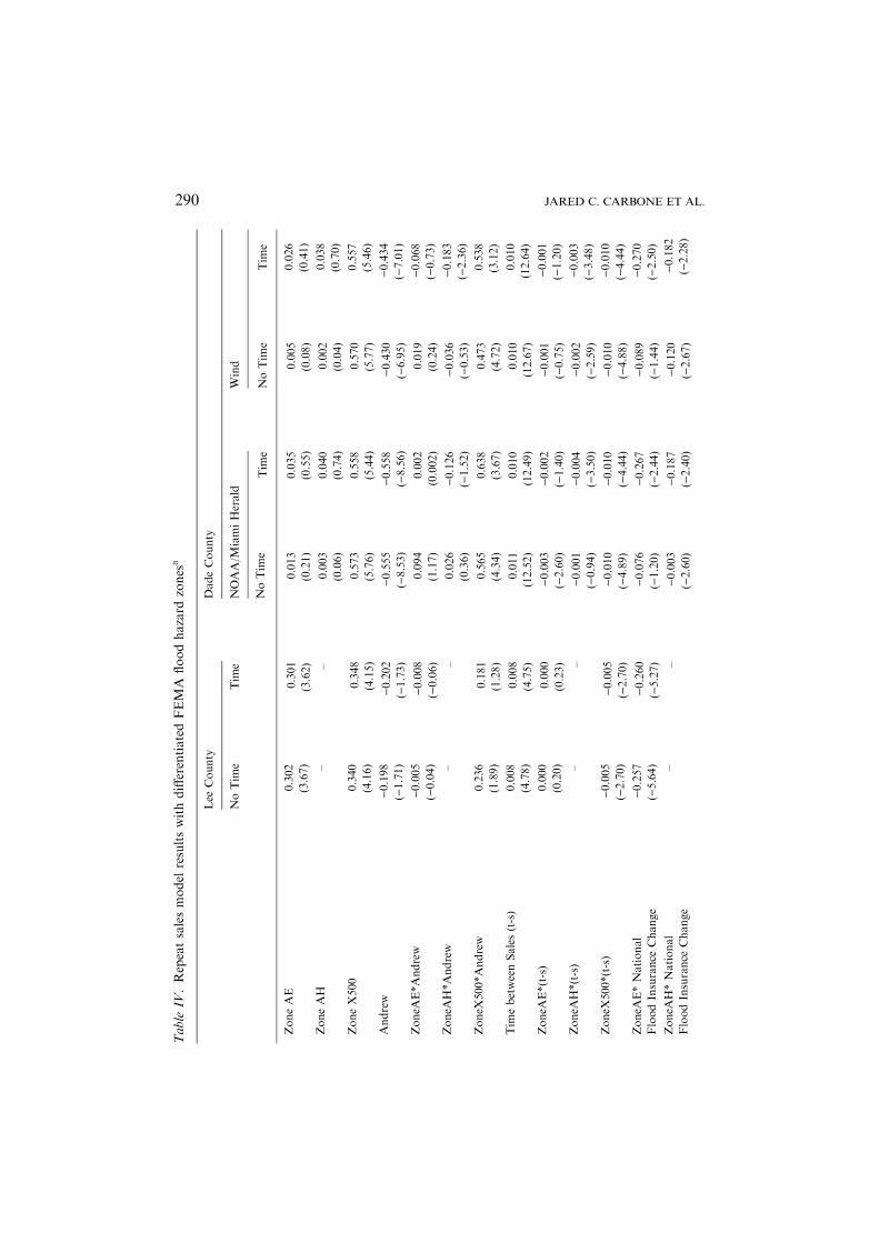
Table III reports our the results with the simplest characterization for theFEMA flood risk zones. Two repeat models are given for Lee County andfour for Dade. The Lee County models are distinguished by whether weallow the effect of Andrew to vary with the months since the hurricane(labeled ‘‘time’’) versus assuming the effect is invariant over time (‘‘no-time’’).These models add to the findings in Hallstrom and Smith (2005), a variablethat evaluates whether the effects of flood insurance are influenced byAndrew. The Dade County models are also distinguished by the treatment oftime and include a further distinction based on how we control for thestorm’s damage. The first two columns repeat the no time/time models usingthe NOAA/Miami Herald damage measure. If the sales bracket Andrew, ithas a value of the proportion of homes designated uninhabitable (zerootherwise) and the last two Dade models used the fixed effect describedearlier to identify areas with high winds for sales that bracket Andrew. Alongthe top of the table we report the estimated DND (difference-in-differences)measure of the effect of Andrew as risk information. For the models allowing


Table

IV.Repeatsalesmodel

resultswithdifferentiatedFEMA

floodhazard

zones

a

Lee

County

DadeCounty

NoTim

eTim

eNOAA/M

iamiHerald

Wind

NoTim

eTim

eNoTim

eTim

e

ZoneAE

0.302

(3.67)

0.301

(3.62)

0.013

(0.21)

0.035

(0.55)

0.005

(0.08)

0.026

(0.41)

ZoneAH

––

0.003

(0.06)

0.040

(0.74)

0.002

(0.04)

0.038

(0.70)

ZoneX500

0.340

(4.16)

0.348

(4.15)

0.573

(5.76)

0.558

(5.44)

0.570

(5.77)

0.557

(5.46)

Andrew

)0.198

()1.71)

)0.202

()1.73)

)0.555

()8.53)

)0.558

()8.56)

)0.430

()6.95)

)0.434

()7.01)

ZoneA

E*Andrew

)0.005

()0.04)

)0.008

()0.06)

0.094

(1.17)

0.002

(0.002)

0.019

(0.24)

)0.068

()0.73)

ZoneA

H*Andrew

––

0.026

(0.36)

)0.126

()1.52)

)0.036

( )0.53)

)0.183

()2.36)

ZoneX

500*Andrew

0.236

(1.89)

0.181

(1.28)

0.565

(4.34)

0.638

(3.67)

0.473

(4.72)

0.538

(3.12)

Tim

ebetweenSales(t-s)

0.008

(4.78)

0.008

(4.75)

0.011

(12.52)

0.010

(12.49)

0.010

(12.67)

0.010

(12.64)

ZoneA

E*(t-s)

0.000

(0.20)

0.000

(0.23)

)0.003

()2.60)

)0.002

()1.40)

)0.001

()0.75)

)0.001

()1.20)

ZoneA

H*(t-s)

––

)0.001

()0.94)

)0.004

()3.50)

)0.002

()2.59)

)0.003

()3.48)

ZoneX

500*(t-s)

)0.005

()2.70)

)0.005

()2.70)

)0.010

()4.89)

)0.010

()4.44)

)0.010

( )4.88)

)0.010

()4.44)

ZoneA

E*National

FloodInsurance

Change

)0.257

()5.64)

)0.260

()5.27)

)0.076

()1.20)

)0.267

()2.44)

)0.089

()1.44)

)0.270

()2.50)

ZoneA

H*National

FloodInsurance

Change

––

)0.003

()2.60)

)0.187

()2.40)

)0.120

()2.67)

)0.182

()2.28)


ZoneX

500*National

FloodInsurance

Change

)0.052

()1.07)

)0.072

()1.53)

)0.010

()4.89)

0.242

(1.18)

0.133

(0.92)

0.234

(1.15)

Andrew*time

–0.002

(0.65)

–0.010

(5.56)

–0.010

(16.02)

ZoneA

E*time*Andrew

–)0.002

()0.57)

–)0.005

()2.15)

–)0.006

()3.06)

ZoneA

H*time*Andrew

––

–)0.003

()1.35)

–)0.003

()2.31)

ZoneX

500*time*Andrew

–0.001

()0.57)

–)0.003

()0.065)

–)0.002

()0.56)

NOAA/M

iamiHearld*Andrew

––

)0.342

()7.78)

)0.336

()7.70)

––

WindBand*Andrew

––

––

)0.345

()10.32)

)0.340

()10.24)

Inverse

MillsRatio

)0.746

()8.73)

)0.745

()8.70)

)1.154

()33.59)

)1.155

()33.70)

)1.140

()33.42)

)1.141

()33.53)

Intercept

0.673

(5.46)

0.674

(5.48)

0.656

(12.42)

0.658

(12.47)

0.650

(12.46)

0.052

(12.48)

Number

ofObservations

5,212

5,212

9,929

9,929

9,929

9,929

R2

0.057

0.057

0.203

0.205

0.208

0.210

ZoneA

E)0.204

(0.00)

)0.201

(0.00)

)0.461

(0.00)

)0.293

(0.00)

)0.411

(0.00)

)0.252

(0.00)

ZoneA

H–

–)0.529

(0.00)

)0.260

(0.00)

)0.466

(0.00)

)0.204

(0.00)

ZoneX

500

0.037

(0.44)

0.065

(0.26)

0.009

(0.94)

0.517

(0.02)

0.043

(0.70)

0.586

(0.00)

aThenumbersin

parentheses

fortheindividiualcoeffi

cientsreferto

theratiooftheestimatedparameter

totherobust(H

uber

1967)estimate

ofthestandard

error.In

thecase

oftestsforrisk

zones

(thelastthreerows)thenumbersin

parentheses

are

p-values

forthetestofnoassociation.Theestimatedeff

ectoftherisk

inform

ation

forthe‘‘notime’’modelsumsthecoeffi

cientforAndrewandAndrew*SFHA.Forthe‘‘time’’modelitalsoincludes

Andrew*SFHA*timewithtimeevaluatedatthe

samplemeanandtreatedasnon-stochastic.ForthemodelsestimatedwiththeDadeCounty

samplethedefinitionsoftheFederalfloodinsurance

variablesinteracted

withthefloodzonefixed

effectsalsoincludeanother

interactionwithavariableidentifyingwhether

thesalesbracket

Andrew.When

theseterm

swereconsidered

for

Lee

county,theindividualparameter

estimatesfortheinsurance

relatedvariableswereinsignificantandtheestimatedeff

ects

attributedto

thestorm

’sinform

ation

wereinsignificant,confirm

ingpopularaccounts

oftheim

mediate

insurance

changes

flowingAndrew

inDadecounty

ascomparedto

other

counties.


the effect to change over time we use the mean number of months betweenAndrew and the most recent sale date.

The hurricane was a statistically significant factor in reducing the rate ofincrease in housing prices in both counties. The effects imply about a 23 to 26percent reduction for Lee County.14 Our findings for this county are con-sistent with interpreting areas with a higher risk of flooding as a proxy forhow homeowners used Andrew as ‘‘news’’ about the risks they faced. Thereare reasons for being cautious because our control for insurance changes islimited. The effects are larger in Dade County. They range from about a 40percent to a 60 percent reduction depending on whether the model controlsfor the time since the sale and how it controls for the storm’s damage. Thus,there is a greater ‘‘weight of evidence’’ supporting the conclusion thathouseholds interpreted the hurricane as an informational signal. Regardlessof how we take account of damage (using the data from the NOAA/MiamiHerald survey or our fixed effect defined by the band associated withAndrew’s path and the locations with the highest wind speeds), the estimatedeffects of the storm on the pace of price changes remain large and statisticallysignificant.

Because the estimated effect of the risk information is especially large forDade County, we may be capturing other changes. Some of this reductionmay be due to insurance changes that popular accounts suggest were pro-nounced in Dade County. We have two variables included to reflect insur-ance changes. The first considers whether the requirement for insurancedifferentially affected properties in SFHA locations. The estimates for bothcounties confirm it did reduce the pace of increase in housing prices. Thesecond term considers whether Andrew impacted this response for allproperties. This effect is insignificant for Lee County but significant andpositive for the Dade County model assuming risk information has a con-stant impact on price changes. This later effect would imply the changes inthe insurance market after Andrew enhanced the appreciation in housingvalues. Given the popular accounts of the insurance changes this conclusionseems unlikely. We are more inclined to conclude our characterization of thiseffect is inadequate. That is, the proxy variable used to control for the effectsof insurance changes is likely to depend on the rating system used to gaugerisks within the special flood hazard areas. To evaluate whether our logic canbe used to recover a differential effect by risk zone within the SFHA sectionsof each county, we re-estimated the model and allowed the hurricane’sinformation to differentially affect each of these zones. These findings aregiven in Table IV.

These models make two changes in the basic specification. Theydecompose the SFHA into zones based on the extent of flood risk with AEthe highest, AH intermediate, and X500 with negligible risk. A fixed effectfor each zone identifies the location of each home. Homes outside any of


these zones provide the control. The second change is to assume that theinsurance change has differential impacts by zone because the insurancerates do vary by zone. There are not sufficient sales in the AH category forLee County to separate this effect so only two risk zones are included inthese models. There are sufficient observations for all three zones to bedistinguished in Dade County. For Dade county, we hypothesize that thezone/insurance change effect is only for homes whose sales bracket Andrewdue to popular accounts suggesting disruption in the insurance marketfollowing the hurricane.

The composite effects of Andrew as risk information are grouped at thebottom of Table IV and they indicate how insurance changes help to explainthe large effects attributed to Andrew for Dade County. When we allow therisk information to vary with time and allow this discrimination in the effectsof the hurricane on insurance, as was implied by our model (see Equation (4))the estimated effects of Andrew in Dade County align more closely with thosefor Lee County in the range of 20–30 percent reduction for the highest riskareas. Moreover, the treatment of the effects of storm damage, whether usingthe Miami Herald measure or the fixed effect for areas with high winds, doesnot change this conclusion.

There was certainly judgment required in formulating our final specifi-cation. As a result, we do not think it is appropriate to cite a simple t-test ofthe difference in measured effects for the two models as confirmation ofapparent consistency in our final estimates. Instead, we believe that theoverall set of findings included in Tables III and IV and support a ‘‘weight ofthe evidence’’ judgment that Hurricane Andrew was a source of new riskinformation for residential housing markets.15

6. Implications

There are a number of reasons for investigating how natural hazards affectpeople’s risk perceptions and behavior. We emphasize their role in providingexogenous risk information to people as quasi-random experiments. In thiscapacity, they can offer analysts the ability to recover estimates of the mar-ginal household’s incremental value for reductions in serious risks of damageand disruption in coastal areas. This extreme event helps in separating riskperception and risk mitigation with a reasonably simple reduced form model.

Nothing ‘‘that good’’ comes without assumptions. In the case of naturalexperiments used for environmental applications, it is often the identificationofa spatially differentiated group that is assumed to experience or notice anoutcome while for others it is either irrelevant or not noticed. This maintainedassumption is difficult to evaluate. Our analysis of Hurricane Andrew in twocounties with a repeat sales framework allowed this assumption to be evalu-ated. One county had no damage from Andrew but was assumed to be close


enough for the residents (and prospective homebuyers) to notice. The other,Dade County, was ‘‘too close’’. It was the site for the worst natural disaster,from the insurance industry’s perspective, in U.S. history. Using extensiverecords on the damage as well as on the path for the storm, we delineate a set ofcontrols that attempt to establish a statistical counterpart to the Lee Countyanalysis.Our findings support the conclusion that households appear to updaterisk perceptions in response to the information provided by the hurricane andthe market effects in proportionate terms are comparable.

Another reason for interest in this type of analysis stems from the eventitself. Severe storms create impacts that can overwhelm local infrastructureand lead to significant disruptions in people’s lives. The time path ofadjustment to the incremental value of the information about storm risk mayoffer indirect evidence of the duration of these adjustment costs and theirmagnitude. Separating these effects will require more information and,potentially, a structural model. The preliminary evidence from Dade Countysuggests models that included a specific treatment of the temporal change inthe effect of Andrew implied a smaller (in absolute magnitude) incrementaleffect. That is, as the date of the most recent sale is further from the date ofthe storm, the absolute size of the composite terms reflecting risk updatingand incremental option price was smaller. These estimates suggest that fur-ther research on this adjustment process is warranted.

Notes

1. Our other research is reported in Hallstrom and Smith (2005) and Smith et al. (2005). Ourframing of the issues discussed in this paper is due in part to comments of the referees and

of Jaren Pope.2. Hurricane Gordon also made landfall in south Florida on November 16, 1994. However,

at the time it crossed the southwest coast of Florida near Fort Myers, it was a tropical

storm. Most of the storm’s damage was due to freshwater flooding of agricultural areas inDade and Collier counties (source: http://www.nhc.noaa.gov/1994gordon.html).

3. Shogren and Crocker (1991, 1999) discuss the prospects for self-protection and self-insurance as influences to the actual risks agents experience. In their framework, the

analyst needs information about the mitigation behaviors jointly adopted with theselocational choices. Smith et al. (2005) use 1990 and 2000 Censuses to offer evidence forDade County that the highest income households seem to be adjusting to storm risk

through insurance and self protection. Middle income households with the economiccapacity to afford relocation seem to take this approach for adjusting.

4. Chay and Greenstone (2005) suggest that the site-specific measures used as sources of

amenities (or risk) in environmental economics are not safely assumed to be exogenous.Endogeneity in the selection of a location can arise from the specific features of uses oractivities that some households may undertake that are unlikely to be known to the

analyst.Their paper is not the first one that has implicitly used a quasi-experimental design to

estimate tradeoffs for environmental amenities and risks. Without using the vocabulary of


quasi-experiments and program evaluation, a number of studies have investigated theeffects of information, policy actions, and time as source of quasi-experimental treatmentsto recover unbiased estimates of these types of tradeoffs. See, for example, Beron et al.

(1997) for the case of earthquakes and Mendelsohn et al. (1992) for hazardous waste sites.In another example of potential problems, Timmins (2003) has argued the rental price

for agricultural land in each use is the maximum of the bid functions and should, inprinciple, reflect the selection process among the alternative uses of each site. His analysis

can be formalized using a random utility model with type one extreme value error todescribe unobserved heterogeneity. In this case, the expected value of the bid, derived asthe maximum of the bids for a given location, will be defined as the log sum rule for a

linear specification of indirect utility. This expression is the approximation he used. As wenote below we assume these effects are avoided with a repeat sales analysis where the focusis on the differential in perceived attributes of a location due to the event. We do not

attempt to measure the factors that caused initial location choices.There is, however, the potential for another type of selection effect due to any special

features of homes that sell more than once. As discussed below we use a sample selectionterm to control for this effect in the models for each county.

5. This development is partially based on a framework discussed in more detail in Hallstromand Smith (2005).

6. Thanks are due to Wally Milon and Richard Ready for calling our attention to this point

as well as for providing some first hand information on the insurance market changes.7. The full expression is actually more complex because a change in insurance rates alters m,

income net insurance expenditures. The details are sufficiently complex to illustrate our

basic point. We cannot separate these components without a structural model so weassumed expenditures were constant.

8. The timing of Andrew is consistent with this premise. It occurred during a lull in hurricane

activity. For much of the preceding decade hurricane activity was at a lower level thanhistory averages (see Goldenberg et al. (2001) and Knutson et al. (1998) for discussion).

9. This formulation adapts Meyer’s (1995) review of the logic of quasi-random experiments.10. See Lewis (2005).

11. We are grateful to Dr. Wakimoto for providing copies of the original maps they preparedto track the storm and helping us to understand them.

12. It was not possible to match the exact subdivision names. To link the Miami Herald data

an ArcView script was developed using a map prepared for the newspaper’s report thatallowed alignment of identified roadways with a GIS map of the country road system. Aset of 306 grids was defined to match damage records to the locations of each property.

Each parcel has a latitude and longitude so once the Miami Herald map was linked to anArcView map of the county these were used to link each property. Thanks are due to JarenPope for implementing this process.

13. The extent to which each record offers complete data varies by county because the data are

derived from county tax records on housing sales. Different counties devote more or lessresources to maintaining the full characteristics of the properties involved in thetransactions.

14. This is approximately comparable to Hallstrom and Smith’s results with a more limitedspecification.

15. We do need to add the caveat that the Lee County results are not necessarily the ‘‘true’’

responses. Local circumstance should be expected to influence responses to riskinformation.


References

AIR Worldwide Corporation, 2002, �Ten Years after Andrew: What Should We Be Preparingfor Now?� AIR Special Report, Technical Document_HASR_0208, August.

Beron, K. J., C. M. James, M. A. Thayer and W. P. M. Vijverberg (1997), ‘An Analysis of the

Housing Market Before and After the 1989 Loma Prieta Earthquake’, Land Economics73(1), 101–113(February).

Chay, K. Y. and M. Greenstone (2003), ‘The Impact of Air Pollution on Infant Mortality:

Evidence from Geographic Variation in Pollution Shocks Induced by a Recession’,Quarterly Journal of Economics 118(August), 1121–1167.

Chay, K. Y. and M. Greenstone (2005), ‘Does Air Quality Matter? Evidence from the HousingMarket’, Journal of Political Economy 113(April), 376–424.

Chivers, J. and N. E. Flores (2002), ‘Market Failure in Information: The National FloodInsurance Program’, Land Economics 78(4), 515–521(November).

Ekeland, I., J. J. Heckman and L. Nesheim (2004), ‘Identification and Estimation of Hedonic

Models’, Journal of Political Economy 112(February), (Part 2)S60–S109.Goldenberg, S. B., C. W. Landsea, A. M. Mestas-Nunez and W. M. Gray (2001), ‘The Recent

Increase in Atlantic Hurricane Activity: Causes and Implications’, Science 293(July), 475–

479.Hallstrom Daniel G. and V. Kerry Smith (2005), ‘Market Responses to Hurricanes’. Journal

of Environmental Economics and Management 50 (November) 541–562.Heckman, J. J. (1979), ‘Sample Selection Bias as a Specification Error’, Econometrica

47(January), 153–161.Huber P. J. (1967), ‘The Behavior of Maximum Likelihood Estimates under Non-Standard

Conditions’, in: Proceedings of the Fifth Symposium on Mathematical Statistics and

Probability. Berkeley. CA: University of California Press.Knutson, T. R., R. E. Tuleya and Y. Kurihara (1998), ‘Simulated Increase of Hurricane

Intensities in a CO2-Warmed Climate’, Science 279(February), 1018–1020.

Lewis R. C. (2005), ‘Insurers drop coastal homes: Hurricane Andrew a key – its claims were 4times higher than other storms’. News & Observer, (March 27).

Longman, P. (1994), ‘The Politics of Wind’, Florida Trend 37(5), 30–39.

Mendelsohn, R., D. Hellerstein, M. Huguenin, R. Unsworth and R. Brayee (1992),‘Measuring Hazardous Waste Damages with Panel Models’, Journal of EnvironmentalEconomics and Management 22(May), 259–271.

Meyer, B. D. (1995), ‘Natural and Quasi-Experiments in Economics’, Journal of Business and

Economic Statistics 12(April), 151–161.Palmquist, R. B. (1982), ‘Measuring Environmental Effects on Property Values without

Hedonic Regressions’, Journal of Urban Economics 11(3), 333–347.

Rappaport (ed.) (1993). Hurricane Andrew 16–28 August, 1992. Preliminary Report, NationalHurricane Center, December.

Rosen, S. (1974), ‘Hedonic Prices and Implicit Markets: Product Differentiation in Perfect

Competition’, Journal of Political Economy 82(February),34–55.Rosenzweig, M. R. and K. I. Wolpin (2000), ‘Natural ‘‘Natural Experiments’’ in Economics’,

Journal of Economic Literature 38(December), 827–874.

Shogren, J. F. and T. D. Crocker (1991), ‘Risk, Self-Protection, and Ex Ante EconomicValue’, Journal of Environmental Economics and Management 20(January), 1–15.

Shogren, J. F. and T. D. Crocker (1999), ‘Risk and Its Consequences’, Journal ofEnvironmental Economics and Management 37(January), 44–51.

Smith V. K., J. C. Carbone, D. G. Hallstrom, J. C. Pope and M. E. Darden (2005), ‘Adjustingto Natural Disasters’, unpublished CEnREP working paper, March 1.


Timmins, C. (2003), ‘Endogenous Land Use and the Ricardian Valuation of Climate Change’,Unpublished Paper, Department of Economics, Yale University, March.

Wakimoto, R. M. and P. G. Black (1994), ‘Damage Survey of Hurricane Andrew and Its

Relationship to the Eyewall’, Bulletin of the American Meteorological Society 75(February),189–200.

Appendix

Appendix A. Probit selection models for housing sales

Year Built Fixed Effect Estimated Parameter

Lee County Dade County

1983 )0.081()0.73)

0.101

(0.87)1984 )0.078

()0.72))0.010()0.09)

1985 )0.298()2.72)

)0.078()0.70)

1986 )0.155()1.47)

)0.055()0.50)

1987 )0.199()1.97)

)0.186()1.73)

1988 )0.240()2.40)

)0.179()1.68)

1989 )0.387()3.92)

)0.303()2.91)

1990 )0.361()3.60)

)0.236()227)

1991 )0.332()3.17)

)0.290()2.71)

1992 )0.308()2.87)

)0.450()4.01)

1993 )0.158()1.54)

)0.864()8.26)

1994 0.165()1.68)

)0.884()8.36)

1995 0.303()3.05)

)0.916()8.42)

1996 0.388

()3.83))0.952()8.77)

1997 0.319()2.95)

)1.237()10.78)

1998 0.079

()0.72))1.118()9.85)

1999 0.013()0.08)

–

Intercept )0.163()1.90)

0.320(3.36)

Number of Observations 8,320 10,534

Pseudo R2 0.0300 0.0712


Can Natural Experiments Measure Behavioral Responses...

Documents

Transcript of Can Natural Experiments Measure Behavioral Responses...