Can Minimum Wages Cause a Big Push? Evidencefrom Indonesia

Jeremy R. Magruder∗

March 16, 2011

Abstract

PRELIMINARY AND INCOMPLETE: PLEASE DO NOT CITEBig Push models suggest that local product demand can create multiple labor mar-

ket equilibria: one featuring high wages, formalization, and high demand and onewith low wages, informality, and low demand. I demonstrate that minimum wagesmay coordinate development at the high wage equilibrium. Using data from 1990sIndonesia, where minimum wages increased in a varied way, I develop a difference inspatial differences estimator which weakens the common trend assumption of differ-ence in differences. Estimation reveals strong trends in support of a big push: formalemployment increases and informal employment decreases in response to the mini-mum wage. Local product demand also increases, and this formalization occurs onlyin the non-tradable, industrializable industries suggested by the model (while em-ployment in tradable and non-industrializable industry also conform to model pre-dictions).

1 Introduction

Wage floors traditionally play a simple role in partial equilibrium models of firm behav-

ior: higher wages imply higher marginal costs, lower labor demand, and lower prof-

its. This simple but powerful intuition has guided a great deal of economic analysis and

intuition regarding the likely effects of externally imposing higher wages, for example

∗University of California, Berkeley. e-mail jmagruder@berkeley.edu. I think Paul Gertler, Ann Harrison,Marieke Kleemans, Alex Rothenberg, and John Strauss for help with various aspects of the data and MichaelAnderson, Alain de Janvry, Ted Miguel, and Elisabeth Sadoulet for several useful discussions. All mistakesare naturally my own.

1

through legal minima. However, if local consumption is an important component of

product demand, then the story quickly becomes much more nuanced. In that event,

higher wages still remain a cost borne by firms; however, they may also increase the size

of the local market which, in turn, can increase either quantities sold or prices and posi-

tively influence profitability and labor demand.

This insight is at the core of classical big push modelling. For example, Rosenstein-

Rodan (1943) suggests that "if... one million unemployed workers were taken from the

land and put... into a whole series of industries which produce the bulk of the goods on

which the workers would spend their wages.... it would create its own additional market,

thus realizing an expansion of world output." Rosenstein-Rodan clarifies: because of this

potential of market formation, wages paid by local firms have the externality of boost-

ing local product demand. The same intuition is formalized in more recent big-push

modelling, such as Murphy, Schleifer, and Vishny (1989; henceforth MSV). MSV demon-

strate that, if workers require a wage premium to supply labor to the formal sector, than

multiple equilibria are possible with industrializing and non-industrializing equilibria

coexisting for some parameter values. In other words, if firm profits are tied to local con-

sumption, then firms create an externality by paying high wages: the size of the market

for other firms increases with worker wages and wealth.

In popular culture, this insight is usually attributed to Henry Ford, who famously

doubled wages at his auto plants to five dollars a day in January 1914. Ford wrote "our

own sales depend on the wages we pay. If we can distribute high wages, then that money

is going to be spent and it will serve to make... workers in other lines more prosperous

and their prosperity is going to be reflected in our sales" (Ford 1922 p. 124-127). The

idea that a firm could unilaterally use wages to increase demand for its own product

enough to offset wage cost seems unlikely and is dismissed by Rosenstein-Rodan (1943),

and Ford’s own statements on the matter were inconsistent (Taylor 2003). As a result,

economists have traditionally interpreted Ford’s wage innovations as an efficiency wage

2

(e.g. Raff and Summers 1989) . However, while it may be not be in a firm’s private in-

terest to pay higher wages, a key intuition of coordinated development is that a firm’s

profits may depend on the wages paid by local firms more generally. This insight was

dubbed the "high wage doctrine" and endorsed by policy makers and economists dur-

ing the great depression, who saw stimulating consumer demand through wages as an

important policy vector to combat the economic downturn (Taylor 2003 extensively doc-

uments the policy discussion). That is, this high wage doctrine reemphasizes this wage

externality. While profits may be decreasing in a firm’s own wages, they may in fact be

increasing in the wages of other nearby firms, which can happen so long as prices do

not fully adjust1. In the MSV modelling, this is achieved through a bisected market of

industrialized high productivity monopolists with prices bounded by a low-productivity

informal fringe, though one can also describe insufficient price adjustment if some goods

are tradable and hence have prices which are unaffected by innovations in local wages2.

In this paper, I add a minimum wage to the MSV big push model, and show that it can

change a multiple-equilibrium setting to one where only the industrialized equilibrium

remains as long as some firms are constrained by the minimum wage. To my knowl-

edge, this is the first paper to explore the consequences of minimum wages in a big push

framework3. I then argue that 1990s Indonesia presents an appropriate case study, as real

minimum wages rose rapidly in a varied way and then dropped quickly with the inflation

rate in the South East Asian financial crash. These changes combine with flexible gov-

ernment policy to create substantial spatial and intertemporal variation in the wage rate.

I develop a difference in spatial differences estimator based on the spatial fixed effects

in Conley and Udry (2010) and Goldstein and Udry (2009) which weakens the standard

1A critique of the high wage doctrine involving the quantity theory of money is presented in Taylor andSelgin (1999). This critique is not relevant to the subnational analysis below.

2Though not pursued here, if consumers have CES utility over tradables and non-tradables, and firmsare competitive with cobb-douglass production, then one can show that so long as tradable and non-tradable goods are sufficiently complementary, the price of tradable goods rises enough in the presenceof minimum wages to motivate increased employment.

3A search of the keywords "minimum wage" and "big push" on econlit turns up zero hits as of 3/1/2011.

3

difference-in-difference identification assumption of similar trends to allow trends to be

non-parametric over time but spatially local. This estimation procedure reveals several

surprising trends which are congruent with a Big Push in Indonesia. First, formal sector

work increases with the minimum wage, while informal sector work decreases, which is

predicted by the MSV model but is the opposite of the prediction a partial equilibrium

analysis would achieve. I also document that local real demand increases, particularly

for non-food items, suggesting that minimum wages are boosting demand, the causal

channel highlighted in the model. The big push model also has strongly heterogeneous

predictions across industries, depending on tradability and industrialization potential.

I look at tradable and non-tradable, formal and informal manufacturing firms to docu-

ment that while the expansion of the formal sector and retraction of the informal sector

are powerful enough trends to be statistically significant for the labor force on average,

they are observed in non-tradable manufacturing but not tradable manufacturing, con-

sistent with model predictions. In contrast, in services (where industrialization potential

is minimal) there is an expansion of informal work, while retail consolidates in response

to rising minimum wages. Finally, I document that trends seem unlikely to be created

through reverse causality or migration and I close by suggesting some explanations for

why these policies may have been successful in 1990s Indonesia, but were widely consid-

ered failures in depression-era America.

2 Model

The model is a straightforward adaptation of Murphy, Schleifer, and Vishny (1989). There

are Q goods, each produced by a distinct industry. A representative consumer has Cobb-

Douglass Utility over these goods, U (x) = ∑Qx=1 ln (x) . In MSV’s original case, each

good could be produced by two production technologies: an informal fringe, which pro-

duces and remunerates at unity, and an industrializing, increasing returns to scale tech-

4

nology which requires an input of F units of labor to access but then can produce α > 1

units with each additional unit of labor. Because the informal fringe will compete away

any prices above unity, prices are fixed at that level.

Finally, MSV suppose that industries feed local demand. With Cobb-Douglass util-

ity, the consumer will spend y/Q on each good; at unit prices this is the production

amount which requires either yQ units of fringe labor or y

αQ + F units of industrialized

labor. Therefore, if the monopolist pays wage w, she earns π profits

π =yQ

(α− w

α

)− Fw (1)

For our purposes, suppose that y is wage income (very similar results are achieved if

y is the sum of wage income and profits). Then, if all firms industrialize,

y =wyα+QFw+ L− y

α−QF (2)

or, solving for y,

y =L+QF (w− 1)(

1−(

w−1α

))Thus, industrialization is profitable for the last firm, if

L+QF (w− 1)

Q(

1−(

w−1α

)) (α− wα

)− Fw > 0 (3)

orLQ

(α− w

α

)> F (4)

If no one industrializes, y = L; thus industrialization is unprofitable for the first firm

ifLQ

(α− w

wα

)< F (5)

5

Which suggests that for certain values of F, there can be multiple equilibria whenever

w > 1.

2.1 Minimum wages and the Big Push

MSV motivate the potential for multiple equilibria from the possibility that workers will

require a wage premium to sell labor to industrializing firms, perhaps because of worse

working conditions or perhaps because of needs related to urbanization. A key point is

that in this model, minimum wages can encourage development. There are two obvious

channels for this to take place:

First, if the equilibrium with no minimum wage is selected, the presence of a minimum

wage may allow coordination at the superior industrializing equilibria. The idea behind

this is simple, and motivated by MSV’s observation that expectations of development

become self-fulfilling in a model like this. Both equilibrium in this model are ex ante

equally sensible. The minimum wage may make formal the expectation that other firms

will pay higher wages, which would push firms towards the industrialized equilibrium.

While I don’t formally develop this equilibrium selection rule here, one might think it

would particularly credible in a time of internationally financed economic growth like

1990s Indonesia.

Second, if the minimum wage can be enforced on some workers in the undeveloped

equilibrium (perhaps because some industries are owned by monopolists but able to op-

erate at low wages, for example, if the wage premium that workers need is heteroge-

neous), then a minimum wage can rule out the undeveloped equilibrium in some para-

meter spaces. Specifically, suppose δL earn the minimum wage, w̄, w̄ ≥ w . As a result,

when the next firm (after the first δ) is considering paying a higher wage, it observes

wage income

δw̄L+ (1− δ) L (6)

6

and is willing to invest if

δw̄L+ (1− δ) LQ

(α− w̄

αw̄

)> F (7)

It is easily verified that there are levels of F such that there would be undeveloped

equilibria without a minimum wage but that there is none with the minimum wage if

δw̄+ (1− δ) >

(α− wα− w̄

)(w̄w

)(8)

So that if the minimum wage successfully binds on at least some workers, then it is

possible for the economy to only allow industrializing equilibria. This is certainly true

locally at w̄ ∼= w, and it is easy to verify that a similar result holds for w̄ < w.

2.2 Industry Heterogeneity

The MSV model, above, assumes that industries are homogeneous. They have two at-

tributes which are important to demand-driven development. First, they are untradable

and their product is consumed locally (that is, they are "articulated" in the language of

de Janvry and Sadoulet (1983). Second, they all have the potential for industrialization.

Homogeneity in these assumptions makes the model transparent and tractable; however,

to develop a broader number of empirical restrictions it is necessary to loosen them. Sup-

pose, therefore, that the MSV modelling assumptions of untradability and potential for

industrialization are relevant for fraction η of industries. Fraction γ are tradable (and all

industrializable). For these firms, demand is not related to local income, thus, they re-

ceive some return R from using γ̃L units of labor which they demand inelastically so long

as they are profitable. 1− γ− η are neither industrializable nor tradable (for example,

services). These industries can only be produced through the informal fringe, and thus

their labor demand is always equal to y/Q.

7

In this scenario, non-tradable, industrializable firms behave very similarly: we now

have two equilibria if

L (1+ γ̃ (w− 1))Qw

(α− w

α

)< F <

L (1+ γ̃ (w− 1))Q (w− η (w− 1))

(α− w

α

)(9)

where the non-industrializable equilibrium can again be ruled out by minimum wages

if there is some compliance. Tradable firms, whose product demand is not subject to local

demand, behave differently: minimum wages evoke either a zero or a negative employ-

ment response. Since the industrialized equilibrium is associated with a higher y than

the non-industrialized firms, this model would suggest that untradable industries which

cannot industrialize increase their labor demand.

2.3 Empirical Predictions

The modelling above highlights the potential of a labor standard to produce demand-

driven development. It also highlights that a broad number of conditions are necessary

for this potential to be realized, including the presence of unutilized technological poten-

tial, the articulation of local firms with consumer demand, and that minimum wages be

appropriately set (one can easily verify that very high minimum wages can serve to elimi-

nate the industrializing equilibrium, as well). In the empirical analysis, I will take several

predictions to the data. First, if minimum wages are inducing big-push-style develop-

ment motivated by local demand, we should observe that formal sector employment in

untradable industries with the potential for industrialization increases while informal sec-

tor employment in these industries decrease in response to an increased minimum wage.

Examining untradable industries with no potential for industrialization, such as services,

we should observe informal sector employment to increase when minimum wages in-

crease. Third, examining tradable industries, we should observe no increase, and poten-

tially a decrease, in formal sector employment in response to minimum wages. Finally,

8

an additional prediction of this modelling is that minimum wages are associated with

growth in local product demand: indeed, this is precisely the mechanism which drives

this model, and one that I will test below.

3 Minimum Wages in Indonesia

The first half of the 1990s was a time of rapid economic expansion in Indonesia. Along-

side this economic expansion, minimum wages grew very quickly in 1990s Indonesia in a

varied way. Commentators suggest that there were two primary pressures which caused

this rise in minimum wages: pressure from the US government, associated with concur-

rent anti-sweatshop activism; and a desire to enforce a national minimum wage which

could purchase a better-than-substistence consumption bundle (see Rama 2001 for a more

extensive discussion). The schedule and timing of these minimum wage increases was

determined by regional tripartite local councils, including representatives of the ministry

of manpower as well as local employers and employees; this procedure led to a varied

growth in minimum wages with 32 different minimum wage regimes countrywide. The

regimes are either provinces or collections of districts within a province. Real minimum

wages (averaged across the country) are presented in figure 1; this graph makes clear that

minimum wages doubled in real terms between 1990 and 1997 before falling as prices

rose alongside the financial crisis. Other studies of these minimum wages (Alatas and

Cameron 2008; Harrison and Scorce 2010; Rama 2001) have used difference-in-differences

or control function approaches and found that these minimum wages reduced employ-

ment, though sometimes only for a subset of firms, and all using data prior to the crisis.

Most similar to this study, Alatas and Cameron (2008) completed a matched difference-

in-differences on firms inside or outside of Jakarta, and found that small firms reduced

employment in response to minimum wages but that there was no effect on large firms.

If these minimum wages fundamentally changed labor markets in Indonesia, it seems

9

necessary that they affected the wage distribution. Given the high level of informality,

we may be concerned about whether minimum wages were in fact enforceable in 1990s

Indonesia. In particular, before turning to employment effects of minimum wages, it is

useful to construct wage histograms to verify both that the minimum wage did distort

the wage distribution, and that this minimum wage was sufficiently high to evoke cred-

ible demand responses. Figure 2 presents the log wage histogram for across years and

Indonesia, where wages are normalized so that 0 indicates a log wage equal to the log

minimum wage in that wage group. Clearly, enforcement is far from perfect, as about a

third of full-time wage workers earn below the minimum in their district. However, there

is also a clear jump in wage densities at the minimum wage, indicating that for some jobs

at least, the minimum wage does affect wages. Analysis below will focus on differences

between nearby districts. Figure 3a and 3b presents minimum wage histograms for indi-

viduals who live within 25 miles of a minimum wage boundary. In Figure 3a, wages are

normalized relative to the minimum in the higher wage regime. In Figure 3b, they are

normalized relative to the minimum in the lower wage regime. As the reader can see,

there is a clear jump in density at the minimum in the own-regime in all cases which is

not present in the alternate wage regime. In other words, people who live nearby each

other but under different minimum wage laws have wages distorted according to their

own laws, so that laws are enforced discontinuously at the border.

4 Empirical Strategy

Employment effects of labor regulation are a traditional topic in economics, and are sur-

veyed in Blau and Kahn (1999); Nickell and Layard (1999); and Freeman (2009) in devel-

oping countries. The majority of these estimates are constructed through either difference-

in-difference style estimators (e.g. Besley and Burgess 2004, Bertrand and Kramarz 2002;

Neumark and Wascher 1992), comparisons across small regions of space (e.g. Dube,

10

Lester, and Reich 2010), or some combination of these two approaches (e.g. Card and

Krueger 1994; Magruder 2010). Dube, Lester, and Reich (2010) summarize the distinc-

tions between these two approaches, which in minimum wage studies in the US have

tended to find small or positive employment effects of minimum wages under close

spatial comparisons and negative employment effects using the difference-in-differences

strategy.

Identification by spatial discontinuity and difference in differences posit two alternate

forms for endogeneity. In either case, the concern is that minimum wage laws are different

in different districts because of some underlying characteristics of the labor market. In

the case of Indonesia, we may be most concerned that the tripartite councils succeeded in

their explicit goals of maintaining similar real wages and that the differences in nominal

minimum wages focus on underlying differences in the price paths of different districts.

Given that local inflation rates seem likely to be related to economic activity, this could

lead to bias in estimation which presumes common trends across treatment and control

areas. A spatial regression discontinuity approach would take advantage of economic

theory suggesting that the capability to trade should render prices and other economic

conditions similar across nearby districts. In this case, nearby labor markets would make

good comparison groups if policy makers target minimum wage policy in response to ag-

gregate labor market characteristics rather than specific characteristics of labor markets

at the borders. The assumption on targeting at the aggregate (policy group) level rather

than the level of individual districts seems appealing and will be tested in the robust-

ness section4. That said, a spatial discontinuity strategy is vulnerable to any differences

4Moreover, since the hypothesized difference is one of local product markets and consumption demand,such an approach also requires that consumption demand is more localized than the confounding marketcharacteristics which minimum wages may be targeted on. Of course, product markets will vary in their lo-calization depending on their tradability, and below empirical restrictions based on this fact are developed.Nonetheless, there is good reason to expect that product markets are sufficiently local, at least for somegoods. The literature has documented that the markets for consumer goods and restaurant are tremen-dously local (with large market shares within five miles) even in the US, where infrastructure is strong andaccess to transport is good (e.g. Anderson and Matsa 2010 for restaurants, Holmes 2009 and Jia 2005 forconsumer goods).

11

between nearby districts, including differences in legislative environments. Difference-

in-difference identification relies on the familiar assumption that trends would remain the

same in the absence of changes in minimum wage law. This assumption seems likely to

hold in Indonesia if the changing time paths of minimum wage are due more to external

pressure or the somewhat arbitrary exercise of bureaucratic power, but is less tenable if

these time paths of policy are indeed the result of careful planning and targeting.

This paper will estimate the effects of minimum wages on employment in three ways.

First, I consider a standard difference-in-difference specification,

yit = αi + δt + β (minwageit) + γXit + εit (10)

where yit is employment in district i in year t, minwageit is the real minimum wage,

and Xit is a vector of controls. As discussed above, this approach will yield consis-

tent estimates of the effects of minimum wages on employment if changes in the mini-

mum wage are unrelated to changes in local labor market conditions. Following, I use

spatial-temporal fixed effects to estimate a spatial discontinuity, following Conley and

Udry (2010), Goldstein and Udry (2009), and Magruder (2010). This procedure allows

minimum wages to be related endogenously to observations, but requires that the endo-

geneity is similar among spatially proximate districts. More specifically, it specifies that

the "true" underlying structural equation is

yit = δt + βminwageit + γXit + νit + εit (11)

where νit is unobserved but related to minwageit and εit is exogenous. The idea behind

this specification is that labor market characteristics at time t are related to the level of the

minimum wage. However, because of the potential for local trade, those characteristics

are similar at time t for other districts within some radius R, so that if we call this set

of districts R (i), then E [νi′t|i′ ∈ R (i) , Xit, minwage] = E [νit|Xit, minwage]. Since every

12

district-year will have a unique radius and unique labor market effect, it is not possible to

represent these effects as a matrix of dummy variables as is conventionally done in fixed

effects analysis. However, we can still treat the spatial effects as nuisance parameters and

estimate the within estimator,

yit − ∑i′∈R(i)

yi′tnR(i)

= β

minwageit − ∑i′∈R(i)

minwagei′tnR(i)

+ γ

Xit − ∑i′∈R(i)

Xi′tnR(i)

(12)

νit − ∑i′∈R(i)

νi′tnR(i)

+ εit − ∑i′∈R(i)

εi′tnR(i)

where nR(i) is the number of district-year observations within radius R of district i.

Since E [νi′t|i′ ∈ R (i) , Xit, minwage] = E [νit|Xit, minwage] , the endogenous component

of the error term disappears in expectation and so if we make an assumption of strict exo-

geneity similar to those used elsewhere in fixed effects analyses (E [εi′t|minwagei′′t, Xi′′t] =

0 ∀i′, i′′ ∈ R (i)), then equation 12 will consistently estimate the effects of minimum wage

law.

Of course, there may be some circumstances in which spatial discontinuity may not

hold. For example, provincial boundaries may be correlated with other legal differences

which affect local labor markets in a discontinuous way, or infrastructure may imperfectly

link two (physically proximate) differences. For this reason, I also estimate a difference

in spatial differences (hence DSD), which loosens the assumptions of both difference-in-

differences and spatial discontinuity estimation. Specifically, I estimate

yit − ∑i′∈R(i)

yi′t =

αi − ∑i′∈R(i)

αι′

+ β

minwageit − ∑i′∈R(i)

minwagei′tnR(i)

(13)

+γ

Xit − ∑i′∈R(i)

Xi′tnR(i)

+ νit − ∑i′∈R(i)

νi′tnR(i)

+ εit − ∑i′∈R(i)

εi′tnR(i)

This approach will be consistent under either the assumptions of difference-in-difference

estimation or the assumptions in spatial discontinuity estimation, and can be understood

13

as a generalization of either. From the perspective of spatial discontinuity, this approach

asks how labor market characteristics are discontinuously different between nearby dis-

tricts in year t as a function of sharp differences in the minimum wage in that year, but

controls nonparametrically for differences between nearby districts which persist over

the length of the panel. From the perspective of difference-in-differences, this approach

loosens the assumption on symmetric trends: rather than requiring districts to have labor

market trends which are unrelated to the presence of minimum wage law (except through

causal mechanisms), this approach allows observations to have non-parametric trends, so

long as those trends are shared among nearby districts (as theory would suggest). Since

this estimation strategy will be consistent whenever either a spatial discontinuity or a dif-

ference in differences produces consistent estimates, these will be my preferred results.

4.1 Standard Errors

The discussion of estimation strategies emphasizes two dimensions of correlation within

observations. First, observations of districts seem likely to be characterized by a seri-

ally correlated component of the error term, which suggests the need for clustering at the

observation level (e.g. Bertrand, Duflo, and Mullainathan 2002). In practice, conven-

tion normally clusters at the level of policy groups. Secondly, the theoretical discussion

suggests that labor markets are similar across small regions of space, suggesting the desir-

ability of spatial clustering (Conley 1999). Moreover, the spatial demeaning will generate

such a correlation even in the absence of an underlying one. Thus, it is important to

cluster over space as well. In practice, I allow observations which are physically close

(with 0.5 degrees latitude and longitude) or in the same policy group in any year to be

related. This is a special case of the Conley (1999) errors, where observations are de-

fined as economically close if they are either physically close or in the same policy group,

and also can be understood as the more computationally intensive procedure outlined in

Cameron, Gelbach, and Miller (2009). Small cluster numbers may be an issue as well,

14

particularly in one of the data sets; I return to this possibility in the Data section.

5 Data

Two data sets are used in this exercise, and summary statistics of the main variables from

each are provided in Table 1. The first data set is waves 1, 2, and 3 of the Indonesia Fam-

ily Life Survey (IFLS), a panel data set which began in 1993 with 7,224 households and

grew to include all a large number of split-off households so that 10,435 households were

interviewed in 2000. Sample selection was completed so that baseline households are rep-

resentative of 83 % of Indonesia’s population. Waves 1, 2, and 3 take place in 1993, 1997,

and 2000. The IFLS is further notable for it’s low attrition rate, with 95% of original house-

holds recontacted in 2000, and over 90% surveyed in all three years. Individual level data

allowed the construction of wage histograms used above, and population-level data will

be useful in allowing measurement of informal economic activity as well as controlling for

demographic changes. Moreover, it will allow control for endogenous migration effects;

thus, we will be able to answer whether individual outcomes change as a result of changes

in minimum wage policy. The second dataset, Statistics Industry, is an annual census of

all manufacturing firms in Indonesia with at least 20 employees collected by the Indone-

sian government statistical agency. Data are aggregated to the district (Kabupaten) level;

coverage includes 209 districts annually for 10 years (1990-2000, with 1997 omitted due to

data unavailability). The manufacturing census has two primary strengths: first, it fully

characterizes formal employment in manufactures over the ten years of coverage. Thus,

we can directly examine formal sector employment using that data. Second, it allows

a great deal of firm-specific data, allowing us to disentangle, for example, employment

in exporting firms from those which serve domestic markets. Employment numbers of

firms in a particular category from these data are therefore the sum of employment across

firms in that category in that district in that year, with zeros imputed for districts where

15

zero firms register with the census. Given that manufacturing firms with greater than 20

workers are legally obligated to register with the census, this imputation seems reason-

able; results which use only the (endogenously changing) sample of districts with positive

employment numbers are available from the author. Interestingly, spatial discontinuity

approaches remain broadly similar using this approach, but difference-in-difference ap-

proaches reveal different estimates, as one would expect if the intertemporal attrition of

districts is representing economically meaningful information. The IFLS sampling proce-

dure excludes some minimum wage groups, so rather than 32 groups of coverage, 21 are

represented in these data. Thirty-two is probably sufficient for cluster asymptotics to rep-

resent reasonable approximations; however, twenty one is small enough that we may be

somewhat concerned. There is an active debate on the robustness of a variety of measures

to prevent overrejection of the null hypothesis in the event of small numbers of clusters,

with Cameron, Gelbach, and Miller (2009) finding simulation evidence that a wild cluster

bootstrap-t test performs best. However, these methods are not extraordinarily familiar,

and haven’t been adapted for multiple non-nested clusters which I argue above are neces-

sary; moreover, Kline and Santos (2011) find less optimistic results for wild bootstraps in

the presence of specification error. I treat this approach as a robustness test and present

p-values from these tests in appendix table 1; most of the primary results are slightly

noisier but still pass conventional statistical significance thresholds. Cameron, Gelbach

and Miller (2009) also find that an ad-hoc approach of using critical values from a tG−2

distribution (where G is the number of clusters) works reasonably well in the range of

20 clusters5. The 1%, 5%, and 10% critical values for a t19 are about 2.87, 2.1, 1.73; as the

reader can verify, the main results of this paper are robust to using these more conserva-

tive critical values. Moreover, the SI, a full coverage census, is not subject to this concern,

and reports similar results.

IFLS and SI geographical locations were determined from actual coordinates of IFLS

5This distribution recalls the results of Donald and Lang (2007), who derive that the tG−2 distribution isin fact the correct distribution under a few specific assumptions.

16

sample communities and internet resources; these are averaged to find district level coor-

dinates. District codes which changed overtime are mapped using the IFLS documenta-

tion supplemented with Olken (2009).

6 Results

The theoretical modelling suggested a number of strong predictions for expected results.

First, and potentially most striking, is that formal sector employment could increase in

response to minimum wage increases, at least for firms which create products which are

not tradable, and which have the potential for industrialization. Nearly as striking, the

big push modelling suggests that these firms should see a reduction in informal employ-

ment, as the formal sector crowds out lower productivity informal work. Here, I under-

take several forms of analysis to test these hypotheses. First, I examine average trends

in formalization and employment; next, I verify that the causal channel of increased local

expenditures does respond to minimum wages; and then I explore industry heterogene-

ity suggested by the model, which provides a set of strong restrictions and requires some

heterogeneity in the nature of labor market evolutions if the big push model is to be be-

lieved.

Both data sets have strengths and weaknesses in terms of trying to identify how the

minimum wage affects the formal and informal sectors. The IFLS, as a population survey,

presents better evidence on what most people are doing in all sectors, including informal

work. While the data do not include identifiers for the legal classification of work,

we can divide workers into full-time wage-earners, part-time wage-earners, and the self-

employed. It seems reasonable to expect that the self-employed are primarily engaged

in informal work, while a greater proportion of full-time workers should be engaged in

formal sector work. Part-time wage-workers may be formally or informally employed.

Thus, we can get some good evidence of the effects of the minimum wage on the informal

17

sector by examining the effects of minimum wages on entrepreneurship, and some less

precise estimates of the effects of minimum wages on formal employment by examining

the effects of minimum wages on full-time wage work, though we will be unsure to the

extent to which this wage work is truly in the formal sector. In contrast, the SI presents a

complete picture of large (greater than 20 employees) manufacturing firms. This includes

some firms which are not legally registered, and thus can provide some evidence on the

informal sector as well. However, the large firm manufacturing sector is likely a very

incomplete picture of informal employment, and so we may view this survey as best po-

sitioned to answer questions about formal employment. Moreover, some manufacturing

products are highly tradable, suggesting that they may not satisfy the assumptions of

untradability where we expected to see these trends.

6.1 Employment Trends

Table 2 presents regressions of various categories of employment on minimum wages us-

ing the IFLS and all three estimation strategies, difference-in-difference (DD), spatial dif-

ference (SD), and difference-in-spatial differences (DSD). For each estimation, I repeat the

spatial estimators at 15, 25, and 50 mile bandwidths to document how estimates change

as we change these (somewhat ad hoc) assumptions. The DSD estimator, which was

the most robust to underlying heterogeneity, shows large positive effects of minimum

wages on full time wage work whenever bandwidths are sufficiently large (and, given

that this procedure does ask a great deal of the data, 25 miles may seem reasonable). The

DSD estimator suggests that a 100% increase in real minimum wages is associated with

approximately a 10% increase in full time waged employment. The SD estimator finds

effects which are similar in sign, though often larger in magnitude as the DSD estimator,

a trend which continues throughout most of the analysis in this paper.

Self Employment provides an opposite trend. The DSD estimator reveals that there is

10-20% less self employment in response to a 100% increase in the minimum wage. Once

18

again, the SD estimates are similar. In contrast, the DD estimates are the opposite sign

and statistically significant. Given that the difference in spatial differences loosens the

difference-in-difference identification assumption, we can infer that the common trends

assumption is inappropriate in this case and that a difference in difference approach could

lead to mistake inference.

The divergence of results between a conventional difference-in-difference strategy and

the difference-in-spatial-differences strategy warrants additional comments. First, it

highlights why results in this study are different from those of previous studies of the

Indonesian minimum wage. Under a common trends assumption, it appears that min-

imum wages are either unchanging or are shrinking formal economic activity, while in-

formal activity is increased (in fact, if samples are restricted to the SI data in the years

considered in Harrison and Scorce (2010), Rama (2001) and Alatas and Cameron (2009),

then the DD estimation reveals negative significant results in formal employment, as it

does in those studies, while DSD estimates are similar to those here). In contrast, when

trends are allowed to differ non-parametrically subject to the restriction that they are spa-

tially local as in the DSD estimation, there is a clear positive effect of the minimum wage

on formal employment and negative effect on informal employment. Given that the DSD

trends assumption is strictly weaker than the DD assumption, so that whenever the DD

estimation is valid, the DSD is as well, we must prefer the DSD estimates. Second,

and more importantly, this divergence speaks directly to whether reverse causality may

be important. Reverse causality in this case would happen if the minimum wage was

carefully targeted at regions with higher secular trends in economic growth. Obviously,

both the DD and the DSD estimates would be robust to targeting on the level of economic

development. Given that the same wage profile is applied to a large regions, if regional

trends were affecting the regional evolution of the minimum wage, we would expect the

positive relationship to show up in the DD estimates most strongly since the DD estimates

reflect the average trends in the purview of the tripartite council. The fact that they show

19

up only in the DSD estimates suggests that if reverse causality is important, it means that

minimum wage profiles are being established for entire regions based on labor market

trends in border districts and not the trends elsewhere in the region, which requires some

specific and curious incentives of politicians. This is strong prima facia evidence that the

effects of the minimum wage documented in this paper are not being driven by reverse

causality, which will be developed further below.

Table 2 suggests that minimum wages are inducing a shift towards formalization of

labor contracts, and potentially a shift towards formalization of economic activity. There

are some limitations to using the IFLS to directly infer whether these new full time work-

ers are employed in the large, formal firms modelled above. Most notably, firm size data

is only available in two of the three survey years, and only coarse (two-digit) occupation

data has been provided to this point (with no industry data provided). Below I’ll use the

fact that some of these occupations do correspond closely to one-digit industries; how-

ever it would be nice to observe whether the new full time wage jobs which are being

created are the sort of job which takes place in formal firms. Here, I use the 1997 and

2000 firm size data to predict the distribution of firm sizes that employ people who work

in each occupation. I then divide these into occupations which tend to work in small firm

occupations (where less than 10% are employed in firms with more than 20 workers), and

large firm occupations with greater than 10% employed in these larger firms. According

to this definition, 57% of workers work in small firm occupations and 43% work in large

firm occupations, and these estimates are robust to alternate sensible definitions. Table

3 presents the results of estimating equation 13 where the dependent variable is work-

ing in a small firm or large firm occupation. The SD and DSD estimates are consistent in

demonstrating that employment is dropping in the types of occupations which work in

small firms and increasing rapidly in the types of occupations which work in large firms

in response to the minimum wage distribution, consistent with a formalization response

to minimum wages.

20

6.2 Market Expansion

The analysis above suggested that employment in the formal sector is increasing in re-

sponse to minimum wage growth. The model suggests that one mechanism for this shift

could be local product demand. Under the big push story, firms internalize local demand,

so that if nearby firms are paying higher wages, then local product markets expand which

provides the impetus for industrial growth. This mechanism is testable. That is, if local

demand is the sponsor for growth, we would expect local consumption to be increasing

along with minimum wages, as well. Here, I use real consumption data from the IFLS.

In particular, I test whether total real expenditures and expenditures on foods or nonfood

products increases in response to minimum wages, where non-food products are defined

as household durables and clothing, products that would be consumed even by relatively

low income wage workers. As a placebo test, I also examine whether food production

changes in response to minimum wages, as local food production is presumably not as-

sociated with demand for the product of local industries.

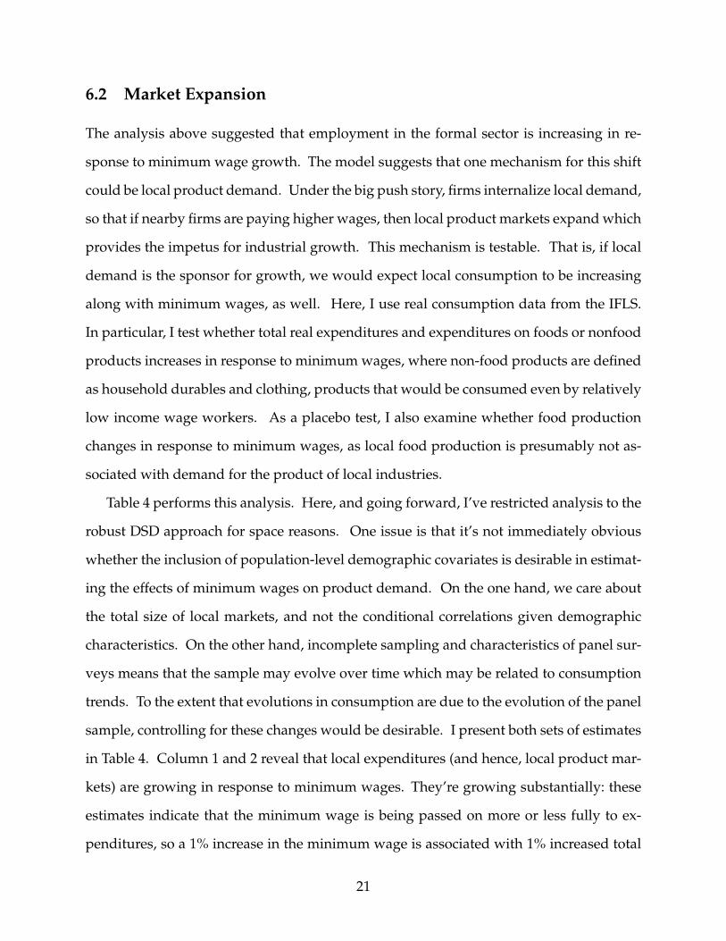
Table 4 performs this analysis. Here, and going forward, I’ve restricted analysis to the

robust DSD approach for space reasons. One issue is that it’s not immediately obvious

whether the inclusion of population-level demographic covariates is desirable in estimat-

ing the effects of minimum wages on product demand. On the one hand, we care about

the total size of local markets, and not the conditional correlations given demographic

characteristics. On the other hand, incomplete sampling and characteristics of panel sur-

veys means that the sample may evolve over time which may be related to consumption

trends. To the extent that evolutions in consumption are due to the evolution of the panel

sample, controlling for these changes would be desirable. I present both sets of estimates

in Table 4. Column 1 and 2 reveal that local expenditures (and hence, local product mar-

kets) are growing in response to minimum wages. They’re growing substantially: these

estimates indicate that the minimum wage is being passed on more or less fully to ex-

penditures, so a 1% increase in the minimum wage is associated with 1% increased total

21

expenditures. Columns (3) and (4) present some weaker evidence that food expenditures

are growing. Without controlling for covariates, we do see a large increase in food expen-

ditures, though in most specifications this increase loses precision once we control for the

population, age, gender distribution, and mean education levels in the district. Columns

(5) and (6) reveal that there is a large increase in non-food consumption which is robust to

the inclusion of covariates. This is reassuring, and strong evidence which speaks to the

plausibility of a big-push: Most industrializable, non-tradable industries produce non-

food goods, and these estimates suggest that their market is indeed expanding6. Finally,

Columns (7) and (8) present a placebo test, looking at food production. Food production

may be reduced in response to minimum wages if workers leave agriculture, but it seems

unlikely that food production would increase with industrialization and better formal

sector labor market opportunities. Reassuringly, the data passes this test, and there is no

statistical relationship between food production and minimum wages.

6.3 Industry Heterogeneity

The model suggested a number of dimensions by which different industries would re-

spond differently to minimum wage law. The primary intuition of the big push model,

that demand creates an externality which can increase formal sector employment which

in turn crowds out the informal sector, is applicable only to industries which were both

untradable (or at least with high costs of trade) and which have the potential for formal-

ization. In contrast, industries which are tradable should experience zero or negative

employment effects from minimum wages. For these firms, there is no externality pro-

duced by other workers increasing the market share, as their product does not specifically

feed the local market. Employment effects may be small if fixed costs are substantial, but

they should not be positive. The second condition, that the potential for formalization

6This trend in non-food consumption recalls the multiplier effects described in Rosenstein-Rodan (1943)and Murphy, Shleifer, and Vishny (1989).

22

exists, was necessary for formal employment to "crowd out" informal employment. Oth-

erwise, if the product is untradable, the externality of increased demand remains, sug-

gesting an increase in labor demand. In industries with low potential for formalization,

that growth will be consigned to the informal sector. These differences amount to strong

empirical restrictions on the data. In principle, comparing across industries is similar to

adding another level of differencing across industries within the data, except that theory

provides stronger predictions on employment patterns than simply that one industry is a

control for another. Here I consider three sectors in turn, for which the model has differ-

ent empirical predictions: Manufacturing, Retail, and Services. In this section, to allow a

number of analyses, I continue to focus on the difference in spatial differences estimator.

6.3.1 Manufacturing

Manufacturing is a sector which includes some tradable and untradable industries (or, at

least, industries where the extent to which markets are local are highly variable). We also

have more complete data about employment trends in manufacturing available in the SI.

The model had few predictions for overall employment trends in an industry like man-

ufacturing which is almost fully industrializable but very heterogeneous in tradability.

Table 5 examines the effects on overall employment in manufacturing and on employ-

ment in registered firms and employment in unregistered firms, using the SI. Though

not shown for space limitations, the SD estimator finds large differences in manufactur-

ing employment. That is, districts with higher minimum wages than their neighbors

tend to have much more manufacturing employment than their neighbors . However,

these effects are not sufficiently robust to survive the DSD procedure, presented in panel

1, suggesting that some of this difference is fixed over time (though the signs are still the

same). Overall, the evidence on an overall effect of minimum wages on manufactur-

ing is similar to the overall trends of increased formal employment, but not very robust

or usually conventionally significant. Similar results are presented in column 2, which

23

examines the probability that there is zero manufacturing employment in a given district.

The SI however contains a tremendous amount of detail about industrial production

and output which can help examine whether these fairly weak estimates are masking

some heterogeneous impacts. Theory would suggest that heterogeneity should be quite

important in an industry like manufacturing: we should see positive employment ef-

fects of minimum wages on non-tradable formal firms, negative employment effects on

non-tradable informal firms, and zero or negative employment effects on tradable firms.

Of course, it is difficult to precisely capture the importance of a local market in a firm’s

output, and as a census of large manufacturing firms, the SI is bound to undersample in-

formal firms. Nonetheless, we can develop proxies for each of these. Here, I suggest that

firms who do not export any of their product are likely to be less tradable and that firms

who export at least some of their production are more likely to be tradable. Moreover, the

SI does include a number of firms (about 25%) who report having no legal status. While

there is likely some misreporting here, we can at least suspect that firms that report no

legal status are more likely to be informal, and that firms who report some legal status

are more likely to be formal. As it turns out, nearly all firms without legal status do not

export, so by these definitions we would conclude that they are not tradable, echoing the

modelling assumptions.

Columns (3) through (5) of Table 5 analyzes the effects of minimum wags on regulated

firms which produce for domestic production, unregulated firms which produce for do-

mestic production, and firms which export (who are nearly all regulated; very similar

estimates are obtained excluding the few unregulated firms who export). The differ-

ence in spatial differences estimator reveals a clear pattern which lines up strongly with

theory: regulated, domestic firms see an increase in employment in response to the mini-

mum wage; unregulated, domestic firms decrease employment; and there is no effect on

exporting firms. Once again, the manufacturing census is revealing a clear pattern: in

response to the minimum wage, formal firms are advantaged relative to informal firms,

24

but only in the case where their product is consumed locally.

Table 6 conducts a similar analysis using the IFLS data. Column (1) finds weak pos-

itive overall effects, as were documented in the SI, and columns (2) and (4) demonstrate

similar patterns to the SI, though they are less precisely estimated. Minimum wages

are increasing the likelihood that individuals are manufacturing wage workers, which is

significant provided the bandwidth is large enough. They are also less likely to be self

employed in manufacturing, though point estimates are small in magnitude and not dis-

tinguishable from zero. Taken together these results are again supportive of an increase in

the formal sector relative to the informal. Columns (3) and (5) of panel (B) looks at wages

and profits in manufacturing. Mean wages are increasing in response to the minimum

wage, as one might anticipate from an industry where much of wage work would be for-

mal (though significance is only marginal). However, profits are not changing among the

individuals who remain entrepreneurs in manufacturing7.

6.3.2 Services

Services are an industry for which industrialization potential is minimal at best. Ser-

vices are also fully untradable. The model suggests therefore that there should be an

increase in labor demand in services. However, that increase in demand should be felt

across the board, not just in the formal sector. That is, since services cannot industrialize,

we shouldn’t observe the crowding out of informal employment that was demonstrated

overall and in manufacturing. Table 7 examines sensitivities of several aspects of services

to minimum wages using data from the IFLS. Column (1) reveals that employment in ser-

vices expands when minimum wages grow, so that a 100% increase in minimum wages

causes approximately 10% greater employment in services. Columns (2) and (4) reveal

that this increase in employment is felt similarly in waged employment and self employ-

ment. In services, both of these are likely informal, though the IFLS does not allow us to

7It is difficult to look at wages in the SI as we only observe total wage bills rather than wages per worker.As such, such analysis is not completed here.

25

determine carefully what fraction of wageworkers and entrepreneurs are formal versus

informal. However, column (3) shows that wages aren’t increasing in services. This is

consistent with the idea that services are fundamentally an informal industry, with little

potential for industrialization and ultimate enforcement (and hence little wage gains in

response to the law). Moreover, column (5) reveals that service profits are growing with

the minimum wage. Along with the growth in service entrepreneurs, this is further evi-

dence that the overall service sector is expanding as entrepreneurs earn greater income.

6.3.3 Retail

It is somewhat less clear what kinds of effects we should anticipate for retail. Clearly, re-

tail is untradable, which means we have a clear prediction that the overall sector should

be growing. However, the extent to which it can be industrialized is much less clear and

with that employment predictions are ambiguous. On the one hand, the retail sector is

clearly different from some manufacturing industries, where one can easily envision the

returns to establishing a large factory. On the other hand, there are clear gains to consoli-

dation in the retail sector, as it is quite clear that the very micro retail establishments which

are commonplace in developing countries are less profitable than the large, horizontally

and vertically integrated retail sector which characterizes much retail in developed coun-

tries. Given this ambiguity, the results presents in table 8 are quite striking. Increased

minimum wages are causing retail employment to contract sharply overall in Indonesia.

Columns (2) and (3) demonstrate that the contraction is largest for self employment, but

still evident for wage work. Of course, the IFLS data can allow only imperfect separation

of formal and informal wage work, and so while it’s fairly clear that informal retail is con-

tracting (since the self employment should be virtually all informal), it is less clear what

is happening to formal retail employment. At the same time, Column (5) reveals that

the total profit bill of retail employment is increasing. Thus, while entrepreneurship in

retail is contracting in response to the minimum wage, the total profits of entrepreneurs

26

are increasing. In other words, the retail sector is consolidating in response to minimum

wages, which is consistent with the formalization results in the other sectors if there are

available returns to scale in retail. Consistent with formalization within retail, Column

(3) documents a growth in wages per worker in response to minimum wages, as well.

7 Robustness

In the analysis above, I identify that local labor markets changed in Indonesia in a way

consistent with the hypothesis that minimum wages were causing a big push. In partic-

ular, formal sector employment increased while informal sector employment decreased.

While this trend is true on average, it is only present (in a statistical sense) in non-tradable,

industrializable industries, while tradable and non-industrializable industries had dif-

ferent trends consistent with the modelling. I also document that local product de-

mand does increase in response to minimum wages, the hypothesized mechanism for

this model. Here, I verify that results are robust to three potential confounders: reverse

causation, prices, and migration.

7.1 Reverse Causation

The primary endogeneity concern in this study is that minimum wages were set accord-

ing to secular trends in labor markets. Of course, the DSD estimation is robust to the

possibility that more developed labor markets received higher minimum wages, but may

be affected if areas are targeted for high minimum wage growth because there is knowl-

edge that they are on a positive growth trend. The fact that a standard difference-in-

difference estimator does not yield the same patterns is a first piece of evidence against

this hypothesis as discussed above: if the tripartite councils are setting real minimum

wages to be the same, and those price differences are correlated with a variety of labor

market characteristics, the trends should be strongest on the raw difference-in-differences

27

which identifies average trends across minimum wage regions rather than the local spa-

tial identification since the councils should be concerned with average outcomes within

their purview. However, it remains possible that border regions are somehow different

from the interior of minimum wages, possibly due to some spurious correlation or some

endogeneity in the chosen minimum wage boundaries, and therefore analysis which fo-

cuses on local comparisons at the border could be affected by reverse causation without

a similar affect being yielded in the raw difference in differences. If this hypothesis were

true, then we would expect to see that minimum wages are closely and differentially re-

lated to employment trends in the border regions. This suggests a simple specification:

yit = αi + δt + β1 (minwageit) + β2 (minwageit ∗ borderi) + γXit + εit (14)

where borderi is an indicator for being within 25 miles of a minimum wage group

border. If the preceding trends of formalization and growth are being driven by reverse

causation, then we should expect that β2 is different from zero and has the same sign as

the DSD estimates above. Table 9 performs this analysis for the key results of tables 2

through 4: the effects of minimum wages on full time wage work, self employment, firm

size, and expenditures. This specification tests whether trends in minimum wages are

correlated with trends in labor market characteristics differentially in border regions.

Column (1) and (2) reveal that there is no statistical difference in minimum wages

based on either general trends in wage work or self employment or any differential re-

lationship with trends in the border regions. In fact, the β2 estimates are opposite in

sign from the preceding estimates, suggesting that if border areas are being targeted in a

differential way, it should go against estimating the striking employment results above.

Column (3) has β2 marginally significant: minimum wages are more positively correlated

with trends in small firm employment in border areas than in interior areas; once again,

this is the opposite sign of the main result and suggests that if we want to interpret this

28

seriously, we should conclude that systematic wage setting is yielding conservative esti-

mates of the effects of minimum wages on small firm growth. Columns (4), (5), and (6)

show no significance in β2, and all columns show no significance in β1. There is therefore

no evidence to suggest that minimum wages are being set in response to labor market

trends, and even less evidence that they are being set differentially at borders in a way

which could yield the estimates contained in this paper. Therefore, if reverse causation is

important in the results presented in this paper, minimum wages are being targeted in a

specific way which is tough to reconcile with sensible policy making: they must be being

targeted at places which have advancing trends relative to their neighbors, but not places

with advancing overall trends. This both requires a great deal of sophistication on the

part of policy makers, and a confusing and hard to identify objective function.

7.2 Prices

As discussed in section 3, one of the key motivations for the variation in minimum wages

was to maintain a constant real wage. This suggests that a concern in analyzing these

minimum wages is whether the estimation strategy does not identify systematic differ-

ences in prices. While it’s not immediately clear what relationship local inflation rates

should have with employment growth in particular sectors, it is clear that if there were

differential inflation associated with the minimum wage, this could lead to misestimates

in the local product demand specification. Since this was the prime support of the

model’s main mechanism, it is important to verify that the DSD technique is not picking

up systematic differences in prices. The presence of trade suggests that prices should be

locally similar which motivated the DSD strategy. However, both of these suggestions

are theoretical rather than empirical, and some evidence would be helpful.

One limitation of the data is that we do not observe the full universe of prices and so

cannot ask how prices of services or non-food items change. However, the IFLS does have

data on food prices for a subset of districts, though these price data are quite variable. In

29

Appendix Table 2, I normalize price data into z-scores and test whether rice, sugar, salt,

and cooking oil prices are associated with real minimum wages8. As the reader can verify,

none have a statistically significant association, and in most specifications point estimates

are actually negative (though standard errors are sometimes large). This is consistent

with the retail sector becoming more efficient as discussed above, and inconsistent with

the idea that the DSD estimation does not adequately control for the relationship between

higher minimum wages and higher inflation. Interestingly, the coefficients on a raw

difference-in-differences (which does not account for spatial trends) are always positive,

though they also do not achieve significance.

7.3 Migration

A second concern with the IFLS is that migration could skew statistics. As a panel

study, the IFLS will reflect trends in the population who were initially surveyed. If in-

dividuals who are well-suited for formal sector work respond to the presence of higher

minimum wages by systematically migrating to high minimum-wage districts, that could

skew employment results (though the presence of jobs for them is still an interesting phe-

nomenon). The first column of table 10 illustrates that individuals do indeed respond to

changes in minimum wage rates by migrating. The dependent variable in this column

is the fraction of individuals in that district-year who entered the panel in a different dis-

trict. At least at the larger bandwidths, there is strong evidence that a larger fraction of

surveyed individuals are migrants when wages are higher than in nearby districts. Im-

mediately, this suggest the potential for bias in estimates due to migration. Fortunately,

it is very possible to perform a robustness analysis. In particular, rather than using a

person’s present location and minimum wage in constructing employment statistics we

can always use the samples’ original districts. That is, we can ignore the information

8The IFLS also has consistent data on fish and beef prices; however, these are frequently non-reported.There are not, any significant relationships between fish and beef prices and minimum wages in the DSDestimator.

30

on their current location and test whether individuals experience changes in type of em-

ployment or overall expenditures based on the minimum wages in the district that they

began the sample in, rather than the district that they currently are in. Column (2) repeats

the migration analysis, but asks this time whether people are more likely to migrate from

their home district based on the home districts minimum wages. If minimum wages are

producing economic opportunities as the analysis above has suggested, we would not

expect an increase in out-migration due to higher minimum wages. Indeed, Column

(2) finds zero effects on outmigration as a result of minimum wage growth, and taken

together, these two columns represent strong evidence that individuals are migrating to

places with higher minimum wages.

The remaining columns of table 10 repeat the analysis of tables 2 and 3, using the

origin-province minimum wages rather than those of the the current province. As the

reader can verify, no results change. That is, even though there is a systematic migration

response to higher minimum wages, this response isn’t the variation that drove analysis

in the previous section. The origin analysis shows that if an individual resides in a district

which expects a future wage profile which is better than nearby neighbors, that individual

can anticipate engaging in the labor force in a more formal way.

8 Discussion and Conclusions

The early 1990s were a time of massive foreign investment and rapid economic growth

for Indonesia. During that time period, the government quickly raised minimum wages.

According to a Big Push Model, if 1990s Indonesia was characterized by the potential

for higher productivity industrial structures, and if the minimum wages were designed

appropriately, then they could achieve a big push - a movement from a low wage, low

consumption, informal labor market to a high wage, high consumption, formal labor mar-

ket. This paper has presented evidence that such a shift did indeed take place. When

31

minimum wages rose in one district relative to their neighbors, that district observed an

increase in formal sector employment and a decrease in informal employment. It also

observed an increase in local expenditures, which is consistent with the hypothesized

mechanism of the big push: that local product demand increases labor demand. More-

over, this increase was only observed in local industries which can be industrialized and

do supply local demand, supporting the model further. Tradable manufacturing firms

saw no growth in employment, and untradable, but non-industrializable services saw an

increase in informal employment.

These trends were identified through a difference in spatial differences analysis, an

approach which weakens the identification assumptions of both difference-in-differences

and spatial discontinuities. This weakening of assumptions was important: a raw difference-

in-differences would have missed these connections. This suggests two things: first, in a

context where labor law is varied, the underlying identification assumptions may be quite

important. In this case, assuming average trends to be the same across districts with dif-

ferent minimum wage profiles would have underestimated employment effects. Second,

it suggests that reverse causality is unlikely to be the explanation for these controver-

sial findings. Minimum wage laws were established for entire regions. If governments

were establishing these varied laws due to variation in the secular trends present in these

regions, then they should have been responding to the average trend present in those

regions, rather than local trends at the borders. Since the raw difference-in-differences

suggests that average trends in employment are not strongly related to the minimum

wage profiles, the potential for reverse causality to be creating these positive estimates is

minimized, and I confirm also that trends at the border are not differentially associated

with minimum wage trends.

This big push discussion strongly recalls much older economic thought which has

been widely discredited within the profession. Few economists today argue as 1920s and

1930s economists did, that increasing wages and local demand could be a motor for eco-

32

nomic growth. One reason is the limited (and potentially negative) effect these policies

had on depression-era America. There are of course many differences between 1990s

Indonesia and 1930s America. One, as a less-developed country receiving substantial

foreign investment, Indonesia may have had new access to potential, unadopted, and

profitable technologies that simply needed a market. A second is that much of the 1990s

were a time of growth in Indonesia, when sticky wages may have limited wage growth

(the opposite of conditions in the depression). Finally, Harrison and Scorce (2010) show

that anti-sweatshop activism also raised labor standards in foreign firms without an ac-

companying drop in employment. This indicates that wages may have indeed been

below marginal products in the 1990s, reducing coordination and creating an opening for

policy. Of course, the analysis employed in this paper cannot determine whether any of

these conditions were important for these results. Further research, both empirical and

theoretical is needed in considering the role of labor standards throughout the business

cycle in modern less developed countries.

References

ALATAS, V., AND L. A. CAMERON (2008): “The Effect of Minimum Wages on Employ-ment in a Low-Income Country: A Quasi-Natural Experiment in Indonesia,” Industrialand Labor Relations Review, 61(2), 201–223.

ANDERSON, M. L., AND D. A. MATSA (2011): “Are Restaurants Really Supersizing Amer-ica?,” AEJ: Applied Economics, 3(1), 152–88.

BERTRAND, M., E. DUFLO, AND S. MULLAINATHAN (2004): “How Much Should We TrustDifference-in-Differences Estimates?,” Quarterly Journal of Economics, 119(1), 249–275.

BERTRAND, M., AND F. KRAMARZ (2002): “Does Entry Regulation Hinder Job Creation?Evidence From the French Retail Industry,” The Quarterly Journal of Economics, 117(4),1369–1413.

BESLEY, T., AND R. BURGESS (2004): “Can Labor Regulation Hinder Economic Perfor-mance? Evidence from India,” The Quarterly Journal of Economics, 119(1), 91–134.

BLAU, F. D., AND L. M. KAHN (1999): “Institutions and Laws in the Labor Market,” inHandbook of Labor Economics, Volume 3, chap. 25, pp. 1399–1461. Elsevier-North Holland.

33

CAMERON, A. C., J. B. GELBACH, AND D. L. MILLER (2006): “Robust Inference withMulti-Way Clustering,” mimeo, University of California, Davis.

CAMERON, C. A., J. GELBACH, AND D. MILLER (2008): “Bootstrap-Based Improvementsfor Inference with Clustered Errors,” Review of Economics and Statistics, 90(3), 414–427.

CARD, D., AND A. B. KRUEGER (1994): “Minimum Wages and Employment: A CaseStudy of the Fast-Food Industry in New Jersey and Pennsylvania,” The American Eco-nomic Review, 84(4), 772–793.

CONLEY, T. G. (1999): “GMM Estimation with Cross-Sectional Dependence,” Journal ofEconometrics, 92(1), 1–45.

CONLEY, T. G., AND C. R. UDRY (2008): “Learning About a New Technology: Pineapplein Ghana,” The American Economic Review, forthcoming.

DE JANVRY, A., AND E. SADOULET (1983): “Social Articulation as a Condition for Equi-table Growth,” Journal of Development Economics, 13(3), 275–303.

DONALD, S. G., AND K. LANG (2007): “Inference with Difference-in-Differences andOther Panel Data,” The Review of Economics and Statistics, 89(2), 221–223.

DUBE, A., T. W. LESTER, AND M. REICH (2010): “Minimum Wage Effects Across StateBorders: Estimates Using Contiguous Counties,” Review of Economics and Statistics,92(4), 945–964.

FORD, H. (1922): My Life and Work. Doubleday, Page, Garden City, NY.

FREEMAN, R. B. (2009): “Labor Regulations, Unions, and Social Protection in DevelopingCountries: Market Distortions or Efficient Institutions?,” NBER Working Paper No.14789.

GOLDSTEIN, M., AND C. UDRY (2008): “The Profits of Power: Land Rights and Agricul-tural Investment in Ghana,” The Journal of Political Economy, forthcoming.

HARRISON, A., AND J. SCORCE (2008): “Multinationals and Anti-Sweatshop Activism,”The American Economic Review, forthcoming.

HOLMES, T. J. (2008): “The Diffusion of Wal-Mart and Economies of Density,” NBERworking paper No. 13783.

JIA, P. (2008): “What Happens When Wal-Mart Comes to Town: An Empirical Analysisof the Discount Industry,” Econometrica, 76(6), 1263–1316.

KLINE, P., AND A. SANTOS (2011): “Higher Order Properties of the Wild Bootstrap UnderMisspecification,” mimeo, Univeristy of California, Berkeley.

MAGRUDER, J. R. (2009): “High Unemployment Yet Few Small Firms: The Role of Cen-tralized Bargaining in South Africa,” mimeo, University of California, Berkeley.

34

MURPHY, K. M., A. SHLEIFER, AND R. W. VISHNY (1989): “Industrialization and the BigPush,” The Journal of Political Economy, 97(5), 1003–1026.

NEUMARK, D., AND W. WASCHER (1992): “Employment Effects of Minimum and Sub-minimum Wages: Panel Data on State Minimum Wage Laws,” Industrial and Labor Re-lations Review, 46(1), 55–81.

NICKELL, S., AND R. LAYARD (1999): “Labor Market Institutions and Economic Perfor-mance,” in Handbook of Labor Economics, Volume 3c, ed. by O. Ashenfelter, and D. Card,pp. 3029–3084. Elselvier-North Holland.

OLKEN, B. A. (2009): “Merged Indonesian Kecamatan Codes,” National Bureau of Eco-nomic Research, electronic data set.

RAFF, D. M. G., AND L. H. SUMMERS (1987): “Did Henry Ford Pay Efficiency Wages?,”Journal of Labor Economics, 5(4, Part 2), S57–S86.

RAMA, M. (2001): “The Consequences of Doubling the Minimum Wage: The Case ofIndonesia,” Industrial and Labor Relations Review, 54(4), 864–881.

ROSENSTEIN-RODAN, P. N. (1943): “Problems of Industrialization of Eastern and South-Eastern Europe,” The Economic Journal, 53(210/211), 202–211.

TAYLOR, J., AND G. SELGIN (1999): “By Our Bootstraps: Origins and Effects of the High-Wage Doctrine and the Minimum Wage,” Journal of Labor Research, 20(4), 447–462.

TAYLOR, J. E. (2003): “Did Henry Ford Mean to Pay Efficiency Wages?,” Journal of LaborResearch, 24(4), 683–94.

35

Variable Obs Mean Std. Dev. Min Max(1) (2) (3) (4) (5)

IFLSMean Full Time Wage Workers 447 0.173 0.100 0.008 0.576Mean Part Time Wage Workers 447 0.037 0.031 0.000 0.216Mean Self Employed 447 0.302 0.111 0.049 0.681

Log Real Minimum Wage (in 1000 Rs) 447 1.196 0.210 0.702 1.672

Mean Workers in Small Firm Occupations 447 0.388 0.183 0.065 0.926Mean Workers in Large Frim Occupations 447 0.270 0.120 0.011 0.722

Mean Workers in Service 447 0.059 0.053 0.000 0.271Mean Wage Workers in Service 447 0.026 0.029 0.000 0.137Mean Self Employed in Service 447 0.022 0.025 0.000 0.123

Mean Workers in Retail 447 0.123 0.068 0.000 0.362Mean Wage Workers in Retail 447 0.029 0.038 0.000 0.286Mean Self Employed in Retail 447 0.146 0.089 0.000 0.565

Mean Workers in Manufacturing 447 0.076 0.059 0.000 0.333Mean Wage Workers in Manufacturing 447 0.043 0.046 0.000 0.242Mean Self Employed in Manufacturing 447 0.026 0.028 0.000 0.200

log Sum Total Expenditures 447 4.786 0.821 2.872 7.250Log Sum Food Purchases 447 4.073 0.748 2.495 6.296Log Sum Non‐Food Purchases 447 4.125 0.892 2.021 6.766Log Sum Food Produced 447 2.106 0.923 0.000 4.584

SILog Production Workers 2090 6.860 2.947 0.000 12.300Indicator for zero workers 2090 0.089 0.285 0.000 1.000Log Registered, Domestic Prod. Workers 2090 6.171 2.942 0.000 11.961Log Unregistered, Domestic Prod. Workers 2090 2.609 2.976 0.000 9.523Log Exporting Workers 2090 1.282 1.353 0.000 5.236

Table 1: Summary Statistics

36

(1)

(2)

(3)

(4)

(5)

(6)

(7)

(8)

(9)

0.03

10.34

6*0.06

40.00

0‐0.008

0.04

60.10

1**

‐0.311

‐0.267

***

(0.043

)(0.198

)(0.079

)(0.013

)(0.057

)(0.049

)(0.044

)(0.122

)(0.046

)

0.27

4***

0.12

7**

‐0.043

**0.01

4‐0.180

***

‐0.206

***

(0.090

)(0.052

)(0.009

)(0.033

)(0.068

)(0.045

)

0.22

2***

0.10

4**

‐0.020

0.00

2‐0.145

**‐0.090

***

(0.078

)(0.048

)(0.019

)(0.028

)(0.058

)(0.029

)

DD

SDDSD

DD

SDDSD

DD

SDDSD

447

447

447

447

447

447

447

447

447

151

151

151

151

151

151

151

151

151

Notes 1

All estim

ates are coe

fficients on

 log real m

inim

um wages whe

re th

e de

pend

ent v

ariable is th

e prop

ortio

n of 

adults who

 work in th

e category given

 in th

e column he

ading

2DD estim

ates present a differen

ce‐in

‐differen

ces; SD estim

ates present a spatia

l discontinuity, and

 DSD

 

estim

ates present a Differen

ce in

 Spatia

l Differen

ces

3Standard  Errors are clustered over space and

 with

in policy grou

ps

4Spatial distances are presumed

 larger th

an bandw

idths for provinces on

 differen

t islands

5Estim

ates con

trol fo

r tim

e tren

ds, urbanization, pop

ulation surveyed

, and

 mean gend

er, age, and

 edu

catio

n

Metho

dN Uniqu

e Districts

Table 2: Employmen

t Effects of M

inim

um W

ages

50 m

iles

Band

width

15 m

iles

25 m

iles

Full Time Wage Work

Part Tim

e Wage Work

Self Em

ploymen

t

37

Table 3: Minimum Wage Effects on Small and Large Firm Occupations

Small Firm Occupations Large Firm Occupations(1) (2) (3) (4) (5) (6)

‐0.026 ‐0.478*** ‐0.458*** 0.125** 0.288** 0.311***(0.069) (0.161) (0.031) (0.062) (0.136) (0.060)

‐0.182 ‐0.438*** 0.095 0.310***(0.170) (0.059) (0.122) (0.073)

25 miles

Small Firm Occupations Large Firm OccupationsBandwidth15 miles

‐0.168 ‐0.360*** 0.123 0.230**(0.137) (0.061) (0.120) (0.099)

DD SD DSD DD SD DSD447 447 447 447 447 447151 151 151 151 151 151

MethodNUnique Districts

50 miles

151 151 151 151 151 151Notes

1 All estimates are coefficients on log real minimum wages where the dependent variable

is the proportion of adults who work in the category in the column heading

2 DD estimates present a difference‐in‐differences; SD estimates present a spatial

discontinuity, and DSD  estimates present a difference in spatial differences

3 Standard Errors are clustered over space and within policy groups

Unique Districts

p p y g p

4 Spatial distances are presumed larger than bandwidths for provinces on different islands

5 Small Firm occupations have fewer than 10% of employees working in firms 

with at least 20 employees, large firm occupations have more than 10%

6 Estimates control for time trends, urbanization, population surveyed, and mean gender

age, and education

38

Table 4: M

inim

um W

ages and

 Expen

ditures

TotalExpen

diture

Food

Purchases

Food

Prod

uctio

nNon

‐Foo

dPu

rchases

(1)

(2)

(3)

(4)

(5)

(6)

(7)

(8)

1.00

8***

0.91

1***

0.72

8**

0.59

41.16

5***

1.15

9***

0.46

31.68

0(0.272

)(0.341

)(0.352

)(0.370

)(0.366

)(0.371

)(2.433

)(2.896

)

1.14

8***

0.79

9***

0.99

3**

0.68

8*1.27

7***

0.95

5***

‐0.544

‐0.207

(0.306

)(0.272

)(0.452

)(0.385

)(0.222

)(0.225

)(2.371

)(2.392

)25

 miles

Band

width

15 m

iles

Total Expen

diture

Food

 Purchases

Food

 Produ

ction

Non

‐Foo

d Pu

rchases

0.58

4*0.31

50.58

9*0.39

30.61

0*0.29

90.40

60.23

6(0.322

)(0.342

)(0.329

)(0.322

)(0.367

)(0.403

)(1.691

)(1.621

)

No

Yes

No

Yes

No

Yes

No

Yes

DSD

DSD

DSD

DSD

DSD

DSD

DSD

DSD

447

447

447

447

447

447

447

447

N50 m

iles

Covariates?

Metho

d44

744

744

744

744

744

744

744

715

115

115

115

115

115

115

115

1Notes 1

All estim

ates are coe

fficients on

 log real m

inim

um wages whe

re th

e de

pend

ent v

ariable is to

tal

log expe

nditu

res in th

e category given

 in th

e column he

ading

2All estim

ates are iden

tified by

 Differen

ce in

 Spatia

l Differen

ces (DSD

)

3Standard Errors are clustered over space and

 with

in policy grou

ps

N Uniqu

e Districts

pp

yg

p

4Spatial distances are presumed

 larger th

an bandw

idths for provinces on

 differen

t islands

5Specificatio

ns includ

ing covariates includ

e mean gend

er, ag, edu

catio

n, and

 the po

pulatio

n surveyed

39

Table 5: Manufacturing Results, SI Data

Log Workers Zero ExportingManufacturing Registered Unregistered

(1) (2) (3) (4) (5)

6.425** ‐0.687*** 7.201*** ‐3.985* 1.584(2.752) (0.204) (2.396) (2.161) (1.340)

Bandwidth

15 miles

Domestic 

0.420 ‐0.304 3.864** ‐2.004** 0.420(0.940) (0.195) (1.825) (0.905) (0.940)

1.128 ‐0.148 1.631* ‐0.300 0.334(1.090) (0.095) (0.948) (0.643) (0.412)

25 miles

50 miles

DSD DSD DSD DSD DSD2090 2090 2090 2090 2090209 209 209 209 209SI SI SI SI SI

Notes

1 All estimates are coefficients on log real minimum wages where the dependent

variable is either log emplyoment in the given category or an indicator for no employment

MethodNUnique DistrictsData

variable is either log emplyoment in the given category or an indicator for no employment

2 All estimates are identified by Difference in Spatial Differences (DSD)

3 Standard Errors are clustered over space and within policy groups

4 Spatial distances are presumed larger than bandwidths for provinces on different islands

40

l f

Table 6: Manufacturing Results, IFLS data

W W k S lf E lTotal Manf.Employment Employment Wages Employment Profits

(1) (2) (3) (4) (5)0.086 0.095 ‐0.091 ‐0.018 0.028(0.057) (0.060) (0.100) (0.043) (0.153)

0.073* 0.085** 0.091* ‐0.011 ‐0.194

Wage Work Self Employment

Bandwidth15 miles

25 miles 0.073 0.085 0.091 ‐0.011 ‐0.194(0.040) (0.034) (0.050) (0.021) (0.142)

0.044 0.070** 0.081* ‐0.018 0.013(0.038) (0.033) (0.047) (0.017) (0.180)

DSD DSD DSD DSD DSDMethod

25 miles

50 miles

447 447 341 447 351151 151 139 151 141IFLS IFLS IFLS IFLS IFLS

Notes

1 All estimates are coefficients on log real minimum wages where the dependent variable

 is either the proportion workingin the given category or log payments

2 All estimates are identified by Difference in Spatial Differences (DSD)

NUnique DistrictsData

2 All estimates are identified by Difference in Spatial Differences (DSD)

3 Standard Errors are clustered over space and within policy groups

4 Spatial distances are presumed larger than bandwidths for provinces on different islands

5 Estimates control for population surveyed, and mean gender, age, and education

41

Employment Employment Wages Employment Profits(1) (2) (3) (4) (5)

0.028 0.083 ‐0.140 0.052 0.806***(0.085) (0.074) (0.122) (0.056) (0.196)

0.096*** 0.0460*** ‐0.080 0.053* 0.878***(0.033) (0.018) (0.096) (0.032) (0.214)

0.096** 0.0348** ‐0.048 0.038* 0.034(0.041) (0.016) (0.064) (0.023) (0.146)

DSD DSD DSD DSD DSD447 447 325 447 279151 151 137 151 146

Notes

1 All estimates are coefficients on log real minimum wages where the dependent variable

 is either the proportion workingin the given category or log payments

2 All estimates are identified by Difference in Spatial Differences (DSD)

3 Standard Errors are clustered over space and within policy groups

4 Spatial distances are presumed larger than bandwidths for provinces on different islands

5 Estimates control for population surveyed, and mean gender, age, and education

MethodNUnique Districts

Table 7: Services

Wage Work Self Employment

25 miles

50 miles

Bandwidth15 miles

42

Employment Employment Wages Employment Profits(1) (2) (3) (4) (5)

‐0.415*** 0.000 0.225*** ‐0.398*** 0.364***(0.047) (0.070) (0.078) (0.048) (0.133)

‐0.299*** ‐0.087* 0.280*** ‐0.266*** 0.325***(0.030) (0.048) (0.059) (0.022) (0.118)

‐0.190*** ‐0.067** 0.155*** ‐0.173*** 0.368***(0.037) (0.027) (0.057) (0.027) (0.124)

DSD DSD DSD DSD DSD447 447 277 447 442151 151 131 151 151

Notes

1 All estimates are coefficients on log real minimum wages where the dependent variable

 is either the proportion workingin the given category or log payments

2 All estimates are identified by Difference in Spatial Differences (DSD)

3 Standard Errors are clustered over space and within policy groups

4 Spatial distances are presumed larger than bandwidths for provinces on different islands

5 Estimates control for population surveyed, and mean gender, age, and education

MethodNUnique Districts

Wage Work Self Employment

25 miles

50 miles

Table 8: Retail

Bandwidth15 miles

43

Full Time

Self

Small Firm

Large Firm

Log Food

 Log Non

‐Foo

dWage Work

Emp

Emp

Emp

Purchases

Purchases

(1)

(2)

(3)

(4)

(5)

(6)

Log Minim

um W

age

0.01

70.11

70.01

60.09

40.13

60.10

5(0.049

)(0.043

)(0.067

)(0.067

)(0.139

)(0.202

)

Border*Log

 ‐0.291

0.39

60.86

2*‐0.533

0.54

81.36

6Minim

um W

age

(0.244

)(0.363

)(0.445

)(0.440

)(1.251

)(1.458

)

DD

DD

DD

DD

DD

DD

447

447

447

447

447

447

151

151

151

151

151

151

Notes 1

All estim

ates are iden

tified by

 Differen

ce in

 Differen

ces (DD)

2Standard Errors are clustered over space and

 with

in policy grou

ps

3Spatial distances are presumed

 larger th

an bandw

idths for provinces on

 differen

t islands

4Estim

ates con

trol fo

r po

pulatio

n surveyed

, and

 mean gend

er, age, and

 edu

catio

n

Table 9: Reverse Causatio

n at th

e Bo

rder

Metho

dObservatio

nsUniqu

e Districts

44

Full Time

Part Tim

eSelf 

Small Firm

Large Firm

InOut

Wage Work

Wage Work

Employmen

tOccup

ations

Occup

ations

(1)

(2)

(3)

(4)

(5)

(6)

(7)

0.10

9‐0.137

0.13

5**

0.00

4‐0.254

***

‐0.512

***

0.31

9***

(0.119

)(0.155

)(0.068

)(0.050

)(0.083

)(0.045

)(0.064

)

0.47

9***

‐0.080

0.11

4**

0.03

9‐0.196

***

‐0.307

***

0.21

9***

(0.076

)(0.107

)(0.048

)(0.040

)(0.038

)(0.052

)(0.065

)

0.35

4***

0.03

10.10

2**

‐0.011

‐0.082

***

‐0.277

***

0.16

4*(0.090

)(0.101

)(0.041

)(0.028

)(0.029

)(0.038

)(0.085

)

Curren

tOrigin

Origin

Origin

Origin

Origin

Origin

DSD

DSD

DSD

DSD

DSD

DSD

DSD

447

449

449

449

449

449

449

151

152

152

152

152

152

152

Notes 1

All estim

ates are coe

fficients on

 log real m

inim

um wages whe

re th

e de

pend

ent v

ariable is indicated in th

e column he

ading

2All estim

ates are iden

tified by

 Differen

ce in

 Spatia

l Differen

ces (DSD

)

3Standard Errors are clustered over space and

 with

in policy grou

ps

4Spatial distances are presumed

 larger th

an bandw

idths for provinces on

 differen

t islands

5Estim

ates  con

trol fo

r po

pulatio

n surveyed

, and

 mean gend

er, age, and

 edu

catio

n

6Cu

rren

t districts are m

eans over the curren

t residen

ce, w

hile origin districts are means over the origin district

Observatio

nsUniqu

e Districts

50 m

iles

District

Metho

d

Migrant Percentage

Table 10

: Migratio

n

Band

width

15 m

iles

25 m

iles

45

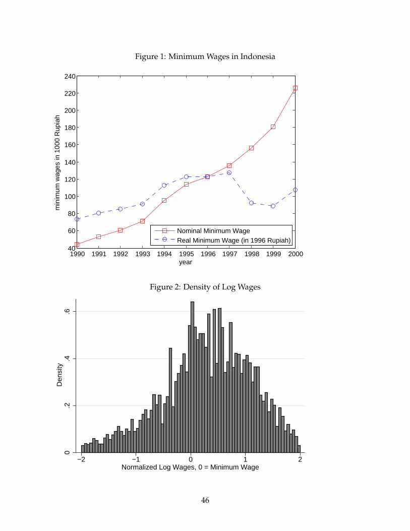
Figure 1: Minimum Wages in Indonesia

1990 1991 1992 1993 1994 1995 1996 1997 1998 1999 200040

60

80

100

120

140

160

180

200

220

240

year

min

imum

wag

es in

100

0 R

upia

h

Nominal Minimum WageReal Minimum Wage (in 1996 Rupiah)

Figure 2: Density of Log Wages

0.2

.4.6

Den

sity

−2 −1 0 1 2Normalized Log Wages, 0 = Minimum Wage

Figure 2: Normalized Wage Density

®

46

Figu

re3:

Wag

eD

ensi

ties

inN

earb

yD

istr

icts

(a)N

orm

aliz

edto

Low

erM

inim

umW

age

0.2.4.6.8Density

−2

−1

01

2N

orm

aliz

ed L

og W

ages

, 0 =

Low

er M

inim

um W

age

Hig

her

Min

imum

Wag

e R

egio

nLo

wer

Min

imum

Wag

e R

egio

n

®

(b)N

orm

aliz

edto

Hig

her

Min

imum

Wag

e

0.2.4.6.8Density

−2

−1

01

2N

orm

aliz

ed L

og W

ages

, 0 =

Hig

her

Min

imum

Wag

e

Hig

her

Min

imum

Wag

e R

egio

nLo

wer

Min

imum

Wag

e R

egio

n

®

Pres

ents

hist

ogra

ms

oflo

gw

ages

whe

reth

esa

mpl

ein

clud

esal

lsub

-dis

tric

tsw

ithi

n25

mile

sof

am

inim

umw

age

bord

er.

Log

wag

esar

eno

rmal

ized

toei

ther

the

high

eror

low

erm

inim

umw

age

47