Can Boundedly Rational Agents Make Optimal Decisions? A...
31
Can Boundedly Rational Agents Make Optimal Decisions? A Natural Experiment. 1 Jonathan B. Berk University of California, Berkeley and NBER and Eric Hughson University of Colorado, Boulder March 2001 This Revision: March 31, 2005 1 The authors would like to thank George Chen for research assistance. A copy of this pa- per is available on the WWW home page http://haas.berkeley.edu/∼berk/. Our respective e-mail addresses are [email protected] and [email protected].
Transcript of Can Boundedly Rational Agents Make Optimal Decisions? A...

Can Boundedly Rational Agents Make Optimal
Decisions?
A Natural Experiment.1
Jonathan B. Berk
University of California, Berkeley and NBER
and
Eric Hughson
University of Colorado, Boulder
March 2001
This Revision: March 31, 2005
1The authors would like to thank George Chen for research assistance. A copy of this pa-per is available on the WWW home page http://haas.berkeley.edu/∼berk/. Our respectivee-mail addresses are [email protected] and [email protected].
Abstract
The television game show The Price Is Right is used as a laboratory to test consis-
tency of suboptimal behavior in an environment with substantial economic incentives.
On the show, contestants compete sequentially in two closely related games. We doc-
ument that contestants who use transparently suboptimal strategies in the objectively
easier game use the optimal strategy almost all of the time in the game that is much
more difficult to solve. Further, there is no consistency in the mistakes that are made
in the two games. One cannot predict, conditional on play in one game, whether play
in the other game will be optimal. The results have implications for the consistency
of behaviorally based economic theory that relies on evidence derived in a laboratory
setting.
1 Introduction
Economists who advocate using fully rational economic models in the presence of
overwhelming evidence that most human beings are boundedly rational often cite
two reasons for their position. First, they point out that often only a few people need
to act in a fully rational way to set prices. The actions of the other people “wash
out,” either because they randomly average to zero, or because of the presence of
arbitrageurs taking advantage of suboptimal behavior. The second reason is more
subtle. Rather than deny that boundedly rational agents have a role in setting prices,
supporters of the rational paradigm argue that the fact that people are incapable of
solving for an optimal rule does not imply that people do not use optimal rules.
Human beings often use optimal decision rules without solving for them explicitly.
For example, a major league pitcher can throw a curve ball without understanding
the physics involved. One might well argue, however, that cases in which such deci-
sion rules are used are usually characterized by situations in which the rule is learned
through experience. Although many economic applications fit this description, oth-
ers do not. In applications in which boundedly rational participants have limited
experience, how likely it that the predictions of an economic model that assumes full
rationality will be useful? The objective of this paper is to provide an answer to this
question by undertaking a natural experiment on the television game show The Price
Is Right.
The answer to this question has implications for economic theory. Although it is
straightforward to find examples where a group of agents behaving suboptimally will
affect the prediction of a fully rational model, actually predicting exactly how their
actions affect the equilibrium can be quite difficult. Predicting suboptimal behavior
depends on whether consistent and predictable patterns of suboptimal behavior exist
and can be detected. Much evidence of this has been found in the laboratory. Re-
searchers have designed experiments that demonstrate consistent suboptimal behavior
in the sense that if the experiment is repeated with different subjects, similar results
obtain. Yet this does not shed much light on the question of immediate relevance to
economists — if these same subjects were instead faced with a real world decision
requiring the kind of skills that they failed to demonstrate in the laboratory, would
their behavior be consistent? The answer to this question has become increasingly
important because recently, many researchers have begun developing non–rationally
based economic models in which the behavioral assumptions are justified based on
1
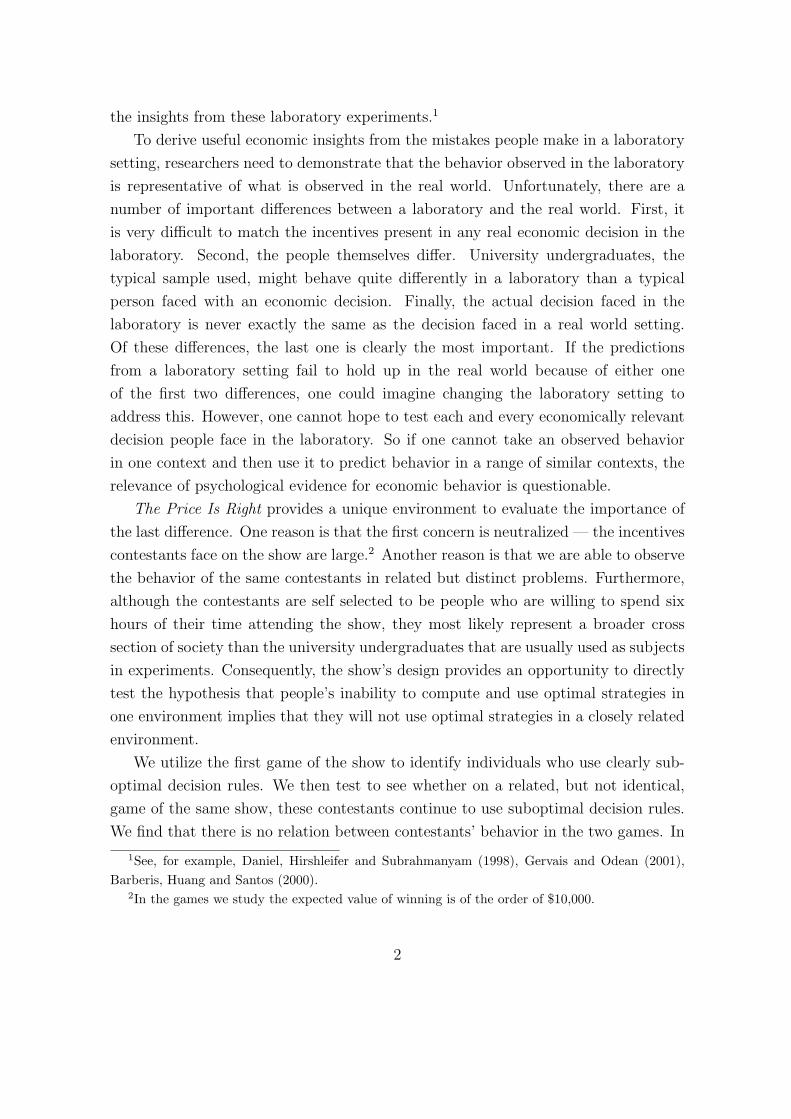
the insights from these laboratory experiments.1
To derive useful economic insights from the mistakes people make in a laboratory
setting, researchers need to demonstrate that the behavior observed in the laboratory
is representative of what is observed in the real world. Unfortunately, there are a
number of important differences between a laboratory and the real world. First, it
is very difficult to match the incentives present in any real economic decision in the
laboratory. Second, the people themselves differ. University undergraduates, the
typical sample used, might behave quite differently in a laboratory than a typical
person faced with an economic decision. Finally, the actual decision faced in the
laboratory is never exactly the same as the decision faced in a real world setting.
Of these differences, the last one is clearly the most important. If the predictions
from a laboratory setting fail to hold up in the real world because of either one
of the first two differences, one could imagine changing the laboratory setting to
address this. However, one cannot hope to test each and every economically relevant
decision people face in the laboratory. So if one cannot take an observed behavior
in one context and then use it to predict behavior in a range of similar contexts, the
relevance of psychological evidence for economic behavior is questionable.
The Price Is Right provides a unique environment to evaluate the importance of
the last difference. One reason is that the first concern is neutralized — the incentives
contestants face on the show are large.2 Another reason is that we are able to observe
the behavior of the same contestants in related but distinct problems. Furthermore,
although the contestants are self selected to be people who are willing to spend six
hours of their time attending the show, they most likely represent a broader cross
section of society than the university undergraduates that are usually used as subjects
in experiments. Consequently, the show’s design provides an opportunity to directly
test the hypothesis that people’s inability to compute and use optimal strategies in
one environment implies that they will not use optimal strategies in a closely related
environment.
We utilize the first game of the show to identify individuals who use clearly sub-
optimal decision rules. We then test to see whether on a related, but not identical,
game of the same show, these contestants continue to use suboptimal decision rules.
We find that there is no relation between contestants’ behavior in the two games. In
1See, for example, Daniel, Hirshleifer and Subrahmanyam (1998), Gervais and Odean (2001),Barberis, Huang and Santos (2000).
2In the games we study the expected value of winning is of the order of $10,000.
2

the earlier game, about half the contestants use transparently suboptimal strategies,
while in the later game, almost every contestant uses the optimal rule. Furthermore,
the few contestants who do depart from the optimal strategy in the later game are
no more or less likely to have used a suboptimal strategy in the earlier game. In
stark contrast to the earlier game, there are so few mistakes on the later game that
every implication of the fully rational model we test is confirmed by the data. What
makes this result particularly surprising is that the second game is significantly more
complex (and difficult to solve) than the earlier game. Contestants who do not use
the optimal decision rule when it is transparent (and when significant losses ensue
as a result), are somehow able to use an optimal decision rule that is much more
complicated to derive and where, paradoxically, the loss for not using the rule is
smaller.
The paper is organized as follows. In section 2, we describe the game show envi-
ronment and detail the two games that contestants play: “Contestants’ Row,” and
“The Wheel Spin.” In section 3, we derive theoretical results. Empirical tests are
performed in section 4. Section 5 discusses the results, and section 6 concludes the
paper.
2 Description of the Game Show
We concentrate on two games played between contestants during the show. The
first game is the initial round of the show called “Contestants’ Row,” in which four
contestants sequentially guess the price of a product displayed on stage. The winner
is the contestant that bids closest without going over. The prize for winning is the
item up for bids as well as the opportunity to play additional games on the show.
We concentrate on the fourth bidder’s bidding behavior. If this contestant uses an
optimal bidding strategy, then he or she will pick one of only four bids — $1 or $1
above any one of the three previous bids. Any other bid is suboptimal because this
contestant can increase her chance of winning by lowering her bid until it becomes
one of these four bids.
This round of the show has been studied by economists before. Both Bennett and
Hickman (1993) and Berk, Hughson and Vandezande (1996) document that about half
of the contestants who bid fourth do not use the optimal decision rule. Furthermore,
not using the rule had real costs. Berk, Hughson and Vandezande (1996) show that
had these contestants used the optimal rule, their likelihood of winning would have
3

risen almost 50%, from 30.6% to 43.2%. In expected value terms this difference is on
the order of $1000.
The second game we study is the “Wheel Spin.” On The Price Is Right, the
“Wheel Spin” is played after “Contestants’ Row” has been played three times and
three different winners have been determined. These three winners spin the wheel,
and a winner is determined. Then, Contestants’ Row is played three more times and
the next three winners play the Wheel Spin game. The two winners of the Wheel
Spin become the two contestants who compete in the final and largest payoff game
of the show, the “Showcase Showdown.”
On the Wheel Spin, the three contestants compete sequentially. The order is
determined by the value of the prizes that each spinner has won up to that point in
the show. The contestant who has won the least spins first, the one who has won the
second–most spins next, and the one who has won the most spins last. The wheel has
20 numbers on it — the numbers from 5 to 100 in intervals of five. Each contestant
may spin the wheel up to two times. After a contestant spins the wheel once, he or
she can either spin again or stop. The contestant’s score is the sum of both spins
if she spins again, or just the first spin if she stops. Once one contestant’s turn is
finished, the next contestant spins. The winner is the contestant who score comes
closest to 100 without going over. If two contestants tie, then each spins once more,
and the contestant with the highest spin wins. If all three contestants tie, then all
three spin once, and the highest spin wins. The expected value of participating in
the Showcase Showdown (winning the wheel spin) is approximately $10,000, which is
similar to the expected value of winning Contestants’ Row, the initial round of the
show.
The strategic choice contestants face on the Wheel Spin is whether or not to spin
again. The advantage of spinning again is that the contestant can potentially increase
his chance of winning by bringing his score closer to 100. The disadvantage is that
he could go over 100 and eliminate himself from the game.
There are a number of additional prizes that can be awarded on the wheel spin.
If any player gets exactly 100 either during their regular play or during a tie breaking
spin, they get an additional $1000 and the chance to spin again. If on this second
spin the player again gets 100 then he gets an additional $10, 000, or if he gets 5 or 15
he gets an additional $5, 000. For most of the paper we will ignore these extra prizes
and consider the chance to compete in the “Showcase Showdown” as the only payoff
of the wheel spin. The effect of including these prizes will be considered in Section 5.
4
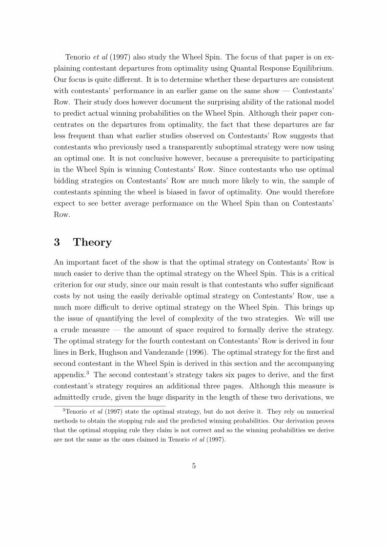
Tenorio et al (1997) also study the Wheel Spin. The focus of that paper is on ex-
plaining contestant departures from optimality using Quantal Response Equilibrium.
Our focus is quite different. It is to determine whether these departures are consistent
with contestants’ performance in an earlier game on the same show — Contestants’
Row. Their study does however document the surprising ability of the rational model
to predict actual winning probabilities on the Wheel Spin. Although their paper con-
centrates on the departures from optimality, the fact that these departures are far
less frequent than what earlier studies observed on Contestants’ Row suggests that
contestants who previously used a transparently suboptimal strategy were now using
an optimal one. It is not conclusive however, because a prerequisite to participating
in the Wheel Spin is winning Contestants’ Row. Since contestants who use optimal
bidding strategies on Contestants’ Row are much more likely to win, the sample of
contestants spinning the wheel is biased in favor of optimality. One would therefore
expect to see better average performance on the Wheel Spin than on Contestants’
Row.
3 Theory
An important facet of the show is that the optimal strategy on Contestants’ Row is
much easier to derive than the optimal strategy on the Wheel Spin. This is a critical
criterion for our study, since our main result is that contestants who suffer significant
costs by not using the easily derivable optimal strategy on Contestants’ Row, use a
much more difficult to derive optimal strategy on the Wheel Spin. This brings up
the issue of quantifying the level of complexity of the two strategies. We will use
a crude measure — the amount of space required to formally derive the strategy.
The optimal strategy for the fourth contestant on Contestants’ Row is derived in four
lines in Berk, Hughson and Vandezande (1996). The optimal strategy for the first and
second contestant in the Wheel Spin is derived in this section and the accompanying
appendix.3 The second contestant’s strategy takes six pages to derive, and the first
contestant’s strategy requires an additional three pages. Although this measure is
admittedly crude, given the huge disparity in the length of these two derivations, we
3Tenorio et al (1997) state the optimal strategy, but do not derive it. They rely on numericalmethods to obtain the stopping rule and the predicted winning probabilities. Our derivation provesthat the optimal stopping rule they claim is not correct and so the winning probabilities we deriveare not the same as the ones claimed in Tenorio et al (1997).
5
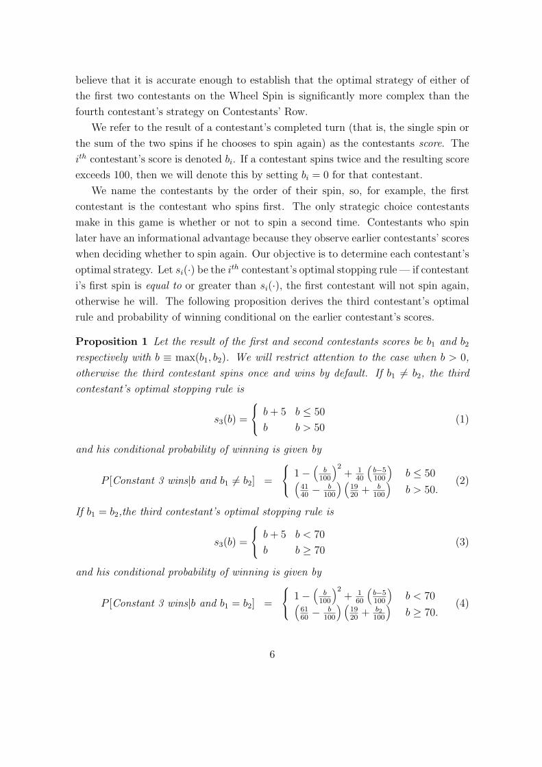
believe that it is accurate enough to establish that the optimal strategy of either of
the first two contestants on the Wheel Spin is significantly more complex than the
fourth contestant’s strategy on Contestants’ Row.
We refer to the result of a contestant’s completed turn (that is, the single spin or
the sum of the two spins if he chooses to spin again) as the contestants score. The
ith contestant’s score is denoted bi. If a contestant spins twice and the resulting score
exceeds 100, then we will denote this by setting bi = 0 for that contestant.
We name the contestants by the order of their spin, so, for example, the first
contestant is the contestant who spins first. The only strategic choice contestants
make in this game is whether or not to spin a second time. Contestants who spin
later have an informational advantage because they observe earlier contestants’ scores
when deciding whether to spin again. Our objective is to determine each contestant’s
optimal strategy. Let si(·) be the ith contestant’s optimal stopping rule — if contestant
i’s first spin is equal to or greater than si(·), the first contestant will not spin again,
otherwise he will. The following proposition derives the third contestant’s optimal
rule and probability of winning conditional on the earlier contestant’s scores.
Proposition 1 Let the result of the first and second contestants scores be b1 and b2
respectively with b ≡ max(b1, b2). We will restrict attention to the case when b > 0,
otherwise the third contestant spins once and wins by default. If b1 6= b2, the third
contestant’s optimal stopping rule is
s3(b) =
b + 5 b ≤ 50
b b > 50(1)
and his conditional probability of winning is given by
P [Constant 3 wins|b and b1 6= b2] =
1−(
b100
)2+ 1
40
(b−5100
)b ≤ 50(
4140− b
100
) (1920
+ b100
)b > 50.
(2)
If b1 = b2,the third contestant’s optimal stopping rule is
s3(b) =
b + 5 b < 70
b b ≥ 70(3)
and his conditional probability of winning is given by
P [Constant 3 wins|b and b1 = b2] =
1−(
b100
)2+ 1
60
(b−5100
)b < 70(
6160− b
100
) (1920
+ b2100
)b ≥ 70.
(4)
6
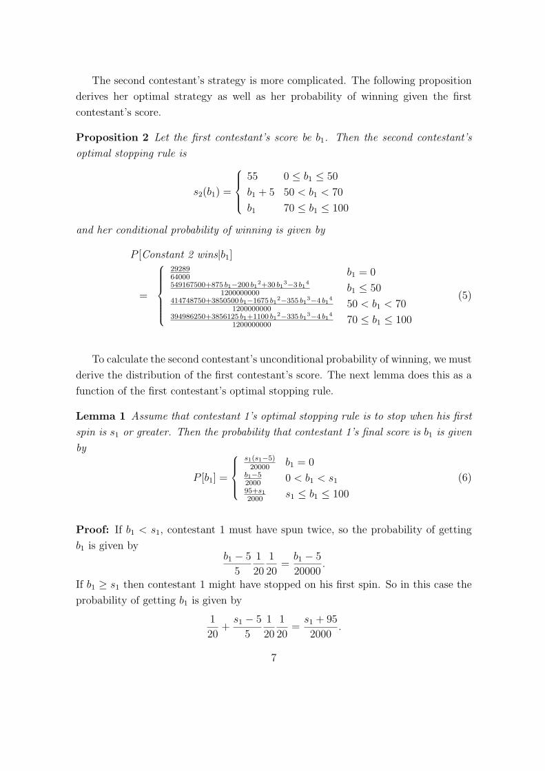
The second contestant’s strategy is more complicated. The following proposition
derives her optimal strategy as well as her probability of winning given the first
contestant’s score.
Proposition 2 Let the first contestant’s score be b1. Then the second contestant’s
optimal stopping rule is
s2(b1) =
55 0 ≤ b1 ≤ 50
b1 + 5 50 < b1 < 70
b1 70 ≤ b1 ≤ 100
and her conditional probability of winning is given by
P [Constant 2 wins|b1]
=
2928964000
b1 = 0549167500+875 b1−200 b1
2+30 b13−3 b1
4
1200000000b1 ≤ 50
414748750+3850500 b1−1675 b12−355 b1
3−4 b14
120000000050 < b1 < 70
394986250+3856125 b1+1100 b12−335 b1
3−4 b14
120000000070 ≤ b1 ≤ 100
(5)
To calculate the second contestant’s unconditional probability of winning, we must
derive the distribution of the first contestant’s score. The next lemma does this as a
function of the first contestant’s optimal stopping rule.
Lemma 1 Assume that contestant 1’s optimal stopping rule is to stop when his first
spin is s1 or greater. Then the probability that contestant 1’s final score is b1 is given
by
P [b1] =
s1(s1−5)20000
b1 = 0b1−52000
0 < b1 < s1
95+s1
2000s1 ≤ b1 ≤ 100
(6)
Proof: If b1 < s1, contestant 1 must have spun twice, so the probability of getting
b1 is given byb1 − 5
5
1
20
1
20=
b1 − 5
20000.
If b1 ≥ s1 then contestant 1 might have stopped on his first spin. So in this case the
probability of getting b1 is given by
1
20+
s1 − 5
5
1
20
1
20=
s1 + 95
2000.
7
Finally, the probability that the first contestant will go over is
1−s1−5
5∑
i=2
5i− 5
2000−
20∑
i=s15
s1 + 95
2000=
s1(s1 − 5)
2000.
•
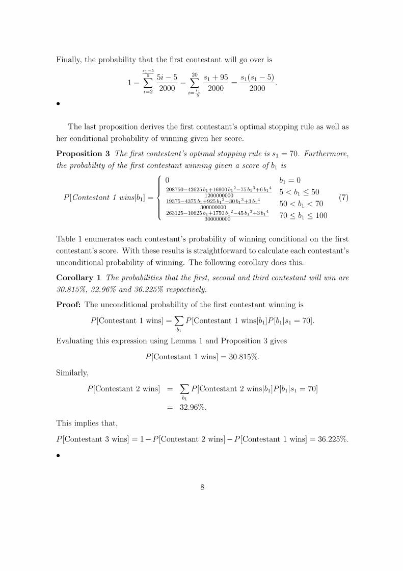
The last proposition derives the first contestant’s optimal stopping rule as well as
her conditional probability of winning given her score.
Proposition 3 The first contestant’s optimal stopping rule is s1 = 70. Furthermore,
the probability of the first contestant winning given a score of b1 is
P [Contestant 1 wins|b1] =
0 b1 = 0208750−42625 b1+16900 b1
2−75 b13+6 b1
4
12000000005 < b1 ≤ 50
19375−4375 b1+925 b12−30 b1
3+3 b14
30000000050 < b1 < 70
263125−10625 b1+1750 b12−45 b1
3+3 b14
30000000070 ≤ b1 ≤ 100
(7)
Table 1 enumerates each contestant’s probability of winning conditional on the first
contestant’s score. With these results is straightforward to calculate each contestant’s
unconditional probability of winning. The following corollary does this.
Corollary 1 The probabilities that the first, second and third contestant will win are
30.815%, 32.96% and 36.225% respectively.
Proof: The unconditional probability of the first contestant winning is
P [Contestant 1 wins] =∑
b1
P [Contestant 1 wins|b1]P [b1|s1 = 70].
Evaluating this expression using Lemma 1 and Proposition 3 gives
P [Contestant 1 wins] = 30.815%.
Similarly,
P [Contestant 2 wins] =∑
b1
P [Contestant 2 wins|b1]P [b1|s1 = 70]
= 32.96%.
This implies that,
P [Contestant 3 wins] = 1−P [Contestant 2 wins]−P [Contestant 1 wins] = 36.225%.
•
8

Table 1: Contestants’ Probability of Winning Conditional on the First Con-
testant’s Score: The first column shows the first contestant’s score (b1). The next three
columns show, respectively, the probability that the first second and third contestant will
win conditional on the score in the first column. The first row of the table is the case when
the first contestant’s score is over 100.
Probability of Winning (%)
b1 1 2 3
Over 0 45.76 54.24
10 0.1215 45.76 54.12
15 0.2852 45.76 53.96
20 0.5397 45.74 53.72
25 0.9065 45.70 53.40
30 1.415 45.62 52.97
35 2.101 45.48 52.42
40 3.009 45.26 51.73
45 4.190 44.94 50.87
50 5.704 44.48 49.82
55 8.346 43.82 47.84
60 11.83 42.60 45.57
65 16.32 40.76 42.93
70 21.56 38.28 40.16
75 28.42 35.21 36.38
80 36.82 31.26 31.92
85 46.99 26.35 26.66
90 59.17 20.36 20.47
95 73.61 13.19 13.21
100 90.57 4.717 4.717
9

4 Empirical Results
We used the same sample of shows used in Berk, Hughson and Vandezande (1996).
The sample consists of 112 broadcasts which were recorded on videotape and then
manually transcribed. A few shows were interrupted by news stories, which left a
total of 767 auctions on Contestants’ Row. In 99 of these auctions all four contestants
overbid, so there were 668 auctions that provided winners. Of the 668 winning bidders,
we have data for 554 contestants who then also spun the wheel, 186 who spun the
wheel first, and 184 each who spun the wheel second and third. The “missing”
contestants (those that won Contestants’ Row but did not spin the wheel) result
from incomplete shows that were interrupted by breaking news stories.4
We begin by calculating the winning percentages on the Wheel Spin and comparing
them to the theoretically predicted values — Table 2. From the table it is clear that
the actual winning percentages are not significantly different to the predicted values.
A similar result obtains when the winning frequency of each number is calculated (see
Table 3). The predictions of the fully rational model cannot be rejected by the data.
These results stand in sharp contrast to what was observed on Contestants’ Row.
There, Berk, Hughson and Vandezande (1996) show that a number of the theoretical
predictions of the fully rational model are rejected by the data.
Table 2: Winning Percentages by Contestant on the Wheel Spin: The
columns show the winning percentages by contestant. In this table we combined
our sample with the numbers reported by Tenorio et al (1997). This increases the
total number of observations to 466. The last row is the p-value, the probability (in
percent) under the Null (that all contestants use the optimal strategy) of observing
a deviation from the theoretical value greater than what is observed.
Winning Probability (%)
1 2 3
Actual 29.83 32.40 37.77
Predicted 30.82 32.96 36.22
p-value 68.32 84.07 45.73
4Part of the time period in which these shows were recored spanned the O.J. Simpson trial.
10

Table 3: Frequency of Each Winning Number: The first column shows the win-
ning contestant’s score. The next column shows the number of occurrences at each score.
There are 184 total occurrences. The next two columns show, respectively, the actual oc-
currence frequency and the theoretical predicted occurrence frequency. The last column is
the p-value, the probability (in percent) under the Null (that all contestants use the optimal
strategy) of observing a deviation from the theoretical value greater than what is observed.
Winning Number Frequency (%) p-value
Score Actual Actual Predicted (%)
≤ 55 9 4.89 4.83 79.47
60 8 4.34 2.19 4.19
65 3 1.63 2.93 42.02
70 7 3.80 5.13 53.65
75 15 8.15 6.98 43.17
80 14 7.61 9.22 54.41
85 25 13.59 11.89 40.39
90 26 14.13 15.05 82.37
95 38 20.65 18.75 44.49
100 39 21.20 23.03 62.31
11

The fact that the winning percentages are not statistically different from their
theoretical values suggest that contestants might be using optimal stopping rules. In
the next subsection we will verify this fact.
4.1 Optimal behavior in the Wheel Spin
Table 4 summarizes the spinning behavior of Price is Right contestants. Almost all
players follow the optimal stopping rule. In the sample of 554 observations, there are
only 21 errors. Not surprisingly, because the third spinner has the easiest decision,
he almost never errs.5 The second spinner made four mistakes, on a much harder
problem.
Table 4: Optimal Behavior by Position on the Wheel Spin: The columns
show the total number of observations (Total), the number of contestants who use
the optimal rule (Optimal), the number that use a suboptimal rule (Suboptimal) and
the percentage of the total who use the optimal rule (Pct. Optimal).
Total Optimal Suboptimal Pct. Optimal
All spinners 186 170 16 91.4
First spinner 184 180 4 97.8
Second Spinner 184 183 1 99.5
The first spinner, who has the hardest problem, still made only 16 mistakes. Given
the first spin, the first spinner’s optimal strategy was, empirically, to stop 65 times
and spin 121. In fact, the first spinner never spun when she should have stopped,
but did stop 16 out of the 121 times she should have spun, or 13.2%. All the errors
consisted of stopping either on 60 (7 times of 12 total spins of 60) or 65 (9 times of 10
total spins of 65). Thus the only systematic mistake we can identify is that a subset
of contestants use 60 or 65 instead of 70 as the optimal stopping rule. However,
the cost of adopting either of these suboptimal rules is trivial. By choosing a policy
of stopping on 65 (60) instead of 70, the first contestant’s unconditional probability
5The single error was a case where the spinner stopped when tied with the first spinner at 45.In that case, spinning yields a probability of winning of 55%, whereas stopping yields a winningpercentage of 50%.
12

of winning drops from 30.82% to 30.74% (30.40%) so the unconditional cost is only
0.08% (0.42%).
Table 5 tabulates the different errors made and the occurrence frequency of error.
It also provides a measure of the conditional cost of the error. That is, the table shows
how much the winning probability would have increased, conditional on the result of
the first spin, had the error not been made and the optimal rule followed instead.6
The cost of the errors made here are substantially smaller than the cost incurred on
Contestants’ Row.7 The only exception is one mistake a second contestant made.
Table 5: Analysis of Errors on the Wheel Spin: This table shows the frequency
of all errors made on the Wheel Spin. The first column describes the type of error made,
the second column show the frequency with which this error occurred in the sample of 554
observations. The final column shows the cost of the error. That is, the column shows by
how much a contestant’s probability of winning (in percent) would have increased had he
used the optimal stopping rule instead.
Description of the Error Frequ. Cost (%)
Contestant 1 stopped on 60 7 6.84
Contestant 1 stopped on 65 9 2.35
Contestant 2 did not stop on 65 (b1 = 45) 1 15.68
Contestant 2 stopped on 65 (b1 = 65) 1 3.66
Contestant 2 stopped on 60 (b1 = 60) 1 8.62
Contestant 2 stopped on 50 (b1 = 0) 1 5.59
Contestant 3 stopped on 45 (max(b1, b2) = 45) 1 5.00
The fact that most contestants use the optimal rule on the Wheel Spin is sug-
gestive that contestants who use the suboptimal rule on Contestants’ Row, use the
optimal rule in the Wheel Spin. It is not conclusive, however, because contestants on
Contestants’ Row who use the optimal bidding strategy are more likely to win. Since
6Although adopting a policy of stopping on 65 (60) instead of 70 makes only a trivial differenceto the unconditional probability of the first contestant winning, the cost of stopping in the subgamewhen the first spin is 65 (60) is non-trivial.
7Berk, Hughson and Vandezande (1996) report that the average winning probability of the fourthbidder would have increased by 13.36% had she used the optimal strategy instead of a suboptimalstrategy.
13

winning on Contestants’ Row is a prerequisite to competing in the Wheel Spin, there
is a selection bias in the sample of contestants on the Wheel Spin in favor of optimal
bidders. In the next subsection we will show, however, that this selection bias is not
responsible for our results.
4.2 Optimal bidding on Contestants’ Row
We define as optimal any bidding strategy that maximizes the probability of winning
Contestants’ Row. As in Berk, Hughson and Vandezande (1996), we define as optimal
any bid made by the fourth bidder that is either a dollar above one of the previous
three bids, or is less than $100.8
We are concerned with optimal bidding behavior over the course of the entire show,
which for some contestants lasts as long as six bidding rounds on Contestants’ Row.
Thus the possibility exists that the same player might use both an optimal bidding
strategy on one round and a suboptimal one on another round on Contestants’ Row.
To classify these contestants, we define a contestant as an optimal bidder if she either
(1) always bid optimally when given a chance to do so as the fourth bidder or (2)
learned to bid optimally after having first bid suboptimally earlier in the show and
then optimally.9 We say that a player bids suboptimally who either (1) always bid
suboptimally when given a chance to do so or (2) bid suboptimally after they have
bid optimally earlier in the show. Last, there are some players, those who never have
the chance to bid as the fourth bidder, about whom we have no information.10
Table 6 summarizes the bidding behavior of Price is Right contestants. Observe
that, as predicted, there is a sample selection bias — bidders who win Contestants’
Row are more likely to have bid optimally (56.8% of winners bid optimally vs. 53%
of all bidders and 43% of non winners). Of the 767 bidding rounds where we know
the winner, we have information about the fourth bidder’s strategy in 764. Of those,
the fourth bidder bid optimally in 389, or 50.9%11 An optimal fourth bid won 168
8In Berk, Hughson and Vandezande (1996), we observe that changing the cutoff rule to, forexample, $5 more than one of the other three bids does not materially affect the results.
9Berk, Hughson and Vandezande (1996) show that the probability that a contestant will bidoptimally increases substantially once another contestant on the same show bids optimally.
10Different definitions of optimality do not appear to materially affect the results. For example,the results did not change when bidders who bid first optimally and later suboptimally were classifiedas “no information.”
11The percentage is lower than the 53% calculated for all bidders because suboptimal bidders aremore likely to lose and hence bid again.
14

Table 6: Optimal Behavior: This table shows the frequency of optimal bidding on
Contestants’ Row and optimal spinning on the Wheel Spin. The columns are the total
number of observations and the strategy used on Contestant Row by the fourth bidder:
Optimal, Suboptimal, and No Information. The last column shows the number of bidders
who used the optimal bidding strategy as a fraction of bidders who we identified as either
optimal or suboptimal. The rows show the results for different partitions of the sample on
both games. The number of spinners does not equal the number of winners of Contestants’
Row because of the existence of missing observations caused by interrupted shows.
Strategy Used on Contestants’ Row
Total Optimal Subopt. No Info. Opt. %
Contestants’ Row:
All bidders 1003 258 229 516 53.0
Winners 668 197 150 321 56.8
Non winners 335 61 79 295 43.6
Wheel Spin:
All Spinners 554 160 117 277 57.8
Spinners who spin correctly 533 153 114 266 57.3
Spinners who err 21 7 3 11 70.0
1st or 2nd spinners 370 107 78 185 57.8
Correct 1st or 2nd spinners 350 100 75 175 57.1
Erring 1st or 2nd spinners 20 7 3 10 70.0
15

of 389 times, or 43.2%; a suboptimal fourth bid won only 99 of 375 times, or only
26.4%.
Table 6 can answer two related questions. First, are optimal bidders on Contes-
tants’ Row more likely to spin correctly? Second, are optimal spinners on the Wheel
Spin more likely to have bid correctly on Contestants’ Row? One might argue that
the third spinner’s problem is transparent, so the table also contains results on the
behavior of just the first and second spinners.
The table confirms that the selection bias is not driving our results. The rea-
son that most contestants on the Wheel Spin use the optimal stopping rule is that
contestants who previously used a suboptimal strategy on Contestants’ Row, use the
optimal stopping rule on the Wheel Spin. Of the 117 contestants who bid subopti-
mally on Contestants’ Row, 114 of them used the optimal stopping rule on the Wheel
Spin.
When we concentrate on the first and second spinners only, we find that optimal
bidders spin correctly 100 of 107 times, or 93.5 %. But suboptimal bidders did even
better, spinning optimally 75 of 78 times, or 96.2% of the time. Optimal spinners bid
correctly 57.1% of the time, insignificantly different from the 57.8% likelihood that
all spinners bid optimally. Finally, suboptimal spinners bid optimally 7 of 10 times,
or 70% of the time (although there were only ten observations). In sum, we find no
evidence that optimal bidders spin better than suboptimal bidders. The reason is, of
course, that bidders spin correctly almost all of the time.12
5 Discussion
We have thus far ignored the effect of bonus payments on the wheel, the extra cash
prizes awarded when a contestant hits 100 exactly. The expected value of getting a
score of 100 is the $1000 paid on that spin as well as the additional possible winnings
from the bonus spin. (Recall that when a contestant gets 100 exactly she is allowed to
spin again.) If the wheel lands on 100 again she wins an additional $10,000, while if
it lands on 15 or 5 she wins an additional $5,000. The only way these bonus payment
can influence the analysis in Section 3 is if they change a contestant’s optimal stopping
rule.
12This is true even when one considers the first and second spinners only. In that case, spinningis optimal 94.6% of the time.
16

Ceteris paribus, the presence of these payments increases the incentive to spin
again. Given a first spin, the expected payoff from possible bonus payments of spin-
ning again is1
20
($1, 000 +
1
20$10, 000 +
2
20$5, 000
)= $100
If the expected value of the Showcase Showdown is $10,000, then this extra payment
adds 1% to the expected payoff the Wheel Spin. If contestants only derive utility
from the monetary rewards, they would be prepared to lower their probability of
winning by up to 1% to spin again for the opportunity of getting a bonus prize. This
number is dwarfed by the cost of spinning again when a first spin gives a result that
the propositions identify as being optimal to stop on.
There is also a countervailing effect. By choosing to spin again the contestant
not only reduces her expected cash reward derived from the chance to appear on
the Showcase Showdown, but also her non–pecuniary reward from appearing on the
Showcase Showdown itself. The Showcase Showdown is the final game of the show
and the entire show builds up to this game. The winner is the “star” of the show
for the day and her family members are allowed to join her on stage at the close of
the show. Although the utility of this is hard to quantify, it is certainly clear that
some fraction of the utility gained by appearing on The Price Is Right is the chance
to appear on national television. The fraction of the total payoffs this comprises
depends on each individual, but given the self selection bias involved, it is difficult
to believe that for most contestants this benefit would comprise less than 1% of the
expected payoff or be worth less than $100. In light of this, the presence of the bonus
payments do not alter contestants’ optimal stopping rules.
It is tempting, given our results, to re–evaluate the complexity of the Wheel Spin.
One could argue that for most results of the first spin, the decision is “obvious.” For
example, it might, in retrospect now appear “obvious” that a first contestant who
say, gets 45, should spin again. As the formal theory in this paper demonstrates,
the actual proof of this fact is complex, time consuming and not obvious at all. It
is certainly harder to derive than the fourth player’s strategy on Contestant’s Row.
Clearly, contestants do not undertake such an analysis — they just seem to know
the optimal rule. Any reader of this article is herself a human being with a similar
cognitive makeup to the contestants on The Price Is Right. Since these contestants
never make this mistake, it is not surprising that a reader of this article would not
either and like the contestants, regard this decision as “obvious.” The interesting, but
at this point, unanswered question is why does a decision that is objectively difficult
17

appear easy?
It is hard to resist speculating about the reasons for our results. The most as-
tonishing fact is the huge disparity in strategies across what a priori appear to be
closely related settings. Why is it that contestants who do not use a transparently
optimal strategy in one game, somehow use a much more complicated optimal strat-
egy in a related game? We believe the answer lies in a puzzle that Berk, Hughson
and Vandezande (1996) note.
It is very likely that the contestants on the The Price Is Right have watched the
show on television prior to appearing as contestants. Since the optimal strategy of
the fourth contestant on Contestants’ Row is clear once you see it, why do people
not learn the strategy from watching the show on television? Furthermore, although
Berk, Hughson and Vandezande (1996) do note a marked increase in the likelihood
that the fourth contestant bids optimally once another contestant on the same show
uses the optimal strategy, 42% of fourth contestants still do not use the strategy.
We conjecture that the reason why so many contestants do not learn the optimal
strategy is that the focus of the game — the amount of the prize — provides little
information about the optimal rule. As on any game show, viewers’ attention is
drawn to the answer so they miss the opportunity to learn the optimal bidding rule.
This is not the case on the Wheel Spin, however. There, the focus of the game, the
winning number, reveals much about the optimal stopping rule. This is because after
watching enough shows, a typical viewer will get some idea of what score is likely
to win, that is, the frequencies in Table 3. As this table makes clear, viewers would
learn that, unconditionally, the probability of the winning score being less than 70 is
low. This information would be very useful in determining when to stop.
Although there is no way to test this hypothesis in on the The Price Is Right itself,
there clearly is some subtle difference between these two games that leads to such
radically different behavior. Such subtle differences have been documented to cause
large changes in outcomes in a laboratory setting. For example, Rapoport, Stein,
Parco, and Nicholas (2001) shows that although in the two–person centipede game,
backward induction fails (see e.g. McKelvey and Palfrey (1992)), in the three person
centipede game, the noncooperative subgame perfect Nash equilibrium emerges after
repeated play between anonymous subjects.
18

6 Conclusion
The important lesson in this paper is that objectively difficult decisions can be cor-
rectly made even by boundedly rational agents. What this implies is that the task of
predicting when boundedly rational agents act suboptimally is complex. One cannot
just take evidence of suboptimality that is derived in a laboratory and assume that
similar behavior will be observed in economic contexts such as financial markets. Yet,
such practice is becoming increasingly common.
The last decade has been characterized by an enormous growth in interest in
economic models that do not rely on assumptions of full rationality. Nowhere is
this more true than in the field of financial economics where the area has de facto
become its own subfield termed Behavioral Finance. Here the field has progressed well
beyond the early models that just assume random departures from rationality (noise
trader models). Today there are numerous examples of financial market equilibria
that are based on explicit models of boundedly rational human behavior. Often, the
motivation for the behavior that is modeled is laboratory evidence. Yet, these papers
provide no evidence that suboptimal behavior that is observed in the laboratory is in
any way predictive of behavior in financial markets.
Behavioral research in the last 40 years has made great strides in studying human
behavior. Mainly as a result of experimental studies, a large body of work exists that
documents consistent and predictable departures in human decision making from
the rational model.13 That is, given the same experimental setup people’s behavior
has been shown to be predictable based on the results of the earlier experiments —
departures from rationality have been shown to be both predictable and consistent.
Based on these results a number of researchers have begun to explicitly incorporate
these departures into economic models. What this paper shows is that one must
be careful when taking results about human behavior that have been derived in
experiments into the real world.
13A review of this literature is beyond the scope of this paper. Interested readers can consultRabin (1998).
19
Appendix
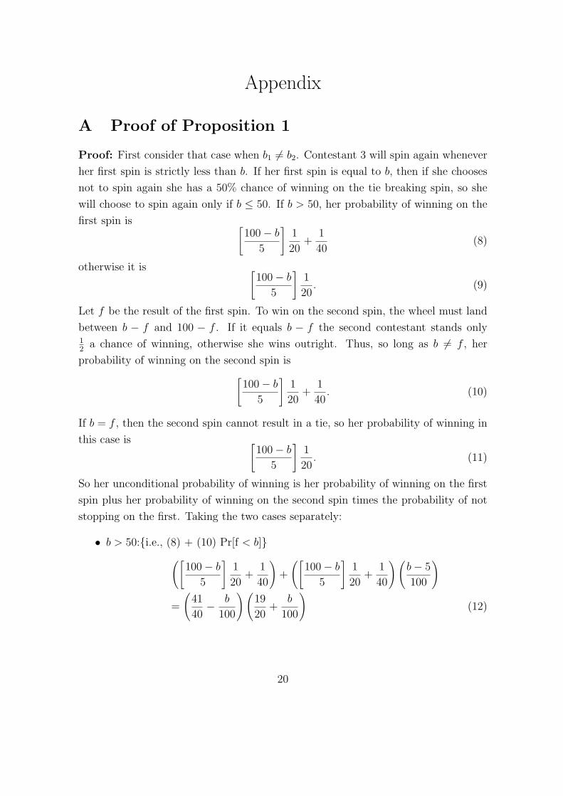
A Proof of Proposition 1
Proof: First consider that case when b1 6= b2. Contestant 3 will spin again whenever
her first spin is strictly less than b. If her first spin is equal to b, then if she chooses
not to spin again she has a 50% chance of winning on the tie breaking spin, so she
will choose to spin again only if b ≤ 50. If b > 50, her probability of winning on the
first spin is [100− b
5
]1
20+
1
40(8)
otherwise it is [100− b
5
]1
20. (9)
Let f be the result of the first spin. To win on the second spin, the wheel must land
between b − f and 100 − f . If it equals b − f the second contestant stands only12
a chance of winning, otherwise she wins outright. Thus, so long as b 6= f , her
probability of winning on the second spin is
[100− b
5
]1
20+
1
40. (10)
If b = f , then the second spin cannot result in a tie, so her probability of winning in
this case is [100− b
5
]1
20. (11)
So her unconditional probability of winning is her probability of winning on the first
spin plus her probability of winning on the second spin times the probability of not
stopping on the first. Taking the two cases separately:
• b > 50:{i.e., (8) + (10) Pr[f < b]}([
100− b
5
]1
20+
1
40
)+
([100− b
5
]1
20+
1
40
) (b− 5
100
)
=
(41
40− b
100
) (19
20+
b
100
)(12)
20

• b ≤ 50: {i.e., (9) + (10) Pr[f < b] + (11) Pr[f= b]}([
100− b
5
]1
20
)+
([100− b
5
]1
20+
1
40
) (b− 5
100
)+
([100− b
5
]1
20
) (1
20
)
= 1−(
b
100
)2
+1
40
(b− 5
100
)(13)
Now consider the case when b1 = b2. As before contestant 3 will spin again whenever
her first spin is strictly less than b. However, in this case if her first spin is equal to
b, then if she chooses not to spin again, since all three contestants will participate in
the tie breaking spin, she has only a 13
chance of winning, so she will choose to spin
again only if b < 70. If b ≥ 70, her probability of winning on the f is[100− b
5
]1
20+
1
60(14)
otherwise it is [100− b
5
]1
20. (15)
If b 6= f probability of winning on the second spin is[100− b
5
]1
20+
1
60. (16)
If b = f , then the second spin cannot result in a tie, so her probability of winning in
this case is [100− b
5
]1
20. (17)
Taking the two cases separately, her unconditional probability of winning is:
• b ≥ 70:{i.e., (14) + (16) Pr[f < b]}([
100− b
5
]1
20+
1
60
)+
([100− b
5
]1
20+
1
60
) (b− 5
100
)
=
(61
60− b
100
) (19
20+
b
100
)(18)
• b < 70: {i.e., (15) + (16) Pr[f < b] + (17) Pr[f= b]}([
100− b
5
]1
20
)+
([100− b
5
]1
20+
1
60
) (b− 5
100
)+
([100− b
5
]1
20
) (1
20
)
= 1−(
b
100
)2
+1
60
(b− 5
100
)(19)
which completes the proof. •
21

B Proof of Proposition 2
Proof: We first calculate the probability of the second contestant getting a particular
b2, given b1 > 0. The probability of observing a b2 such that s2(b1) ≤ b2 ≤ 100 is
equal to the probability of getting b2 on the first spin plus the probability of getting
b2 after both spins times the probability of not stopping:
P [b2|s2(b1) ≤ b2 ≤ 100] =1
20+
[s2(b1)− 5
100
]1
20. (20)
If b2 < s2(b1), then it must have taken 2 spins so the probability of observing this is
P [b2|b2 < s2(b1)] =
[b2 − 5
100
]1
20. (21)
When contestant 2 has beaten contestant 1’s score, his probability of winning is just
the complement of contestant 3’s probability of winning. Thus, from Proposition 1
we have
P [Contestant 2 wins|b2 and b1 < b2] =
(b2100
)2+ 1
40
(b2−5100
)b ≤ 50
1−(
4140− b2
100
) (1920
+ b2100
)b > 50.
and
P [Contestant 2 wins|b2 and b1 = b2] =
12
[(b2100
)2+ 1
60
(b2−5100
)]b ≤ 70
12
[1−
(6160− b2
100
) (1920
+ b2100
)]b > 70.
We will leave it to the reader to verify that s2(b1) > 50 when b1 ≤ 50. Contestant 2’s
probability of winning, given that b1 ≤ 50 < s2(b1).
P [Constant 2 wins|b1]
=∑
b2
P [Contestant 2 wins|b2, b1 and b1 ≤ b2]P [b2|s2(b1)]
=10∑
i=b1+5
5
((5i
100
)2
− 1
40
(5i− 5
100
)) [5i− 5
100
]1
20
+
s2(b1)−5
5∑
i=11
(1−
(41
40− 5i
100
) (19
20+
5i
100
)) [5i− 5
100
]1
20
+20∑
i=s2(b1)
5
(1−
(41
40− 5i
100
) (19
20+
5i
100
)) (1
20+
[s− 5
100
]1
20
)
22

+1
2
(b1
100
)2
− 1
60
(b1 − 5
100
)
[b1 − 5
100
]1
20
=1
1200000000(394686250 + 875 b1 − 200 b1
2 + 30 b13 − 3 b1
4 (22)
+ 3812500 s2(b1) + 5950 s2(b1)2 − 385 s2(b1)
3 − s2(b1)4).
If 70 > s2(b1) > b1 > 50, then
P [Constant 2 wins|b1]
=
s2(b1)−5
5∑
i=b1+5
5
(1−
(41
40− 5i
100
) (19
20+
5i
100
)) [5i− 5
100
]1
20
+20∑
i=s2(b1)
5
(1−
(41
40− 5i
100
) (19
20+
5i
100
)) (1
20+
[s− 5
100
]1
20
)
+1
2
(b1
100
)2
− 1
60
(b1 − 5
100
)
[b1 − 5
100
]1
20
=1
1200000000(395611250 + 2875 b1 + 1300 b1
2 + 50 b13 − 3 b1
4 (23)
+ 3812500 s2(b1) + 5950 s2(b1)2 − 385 s2(b1)
3 − s2(b1)4)
Taking the derivative of either (22) or (23) with respect to s2(b1) provides:
3812500 + 11900 s2(b1)− 1155 s2(b1)2 − 4 s2(b1)
3
1200000000. (24)
Setting this expression equal to zero and solving gives s2(b1) = 56.98. It is easy to
verify that (22) and (23) are maximized for s2(b1) = 55, since the expressions are
concave and s2(b1) = 60 provides a lower value. Thus, s2(b1) = 55 is the optimal
stopping rule when b1 < 55.
When b1 > 55, it is clearly suboptimal to stop at 55. However, what is not clear
is whether it is optimal to stop at b1 or at b1 + 5. When 55 ≤ b1 < 70 we have
P [Constant 2 wins|b1 and s2(b1) = b1]
=20∑
i=b1+5
5
(1−
(41
40− 5i
100
) (19
20+
5i
100
)) (1
20+
[b1 − 5
100
]1
20
)
+1
2
(b1
100
)2
− 1
60
(b1 − 5
100
)
(1
20+
[b1 − 5
100
]1
20
)
=394036250 + 3860375 b1 + 1250 b1
2 − 335 b13 − 4 b1
4
1200000000(25)
23

or
P [Constant 2 wins|b1 and s2(b1) = b1 + 5]
=20∑
i=b1+5
5
(1−
(41
40− 5i
100
) (19
20+
5i
100
)) (1
20+
[b1
100
]1
20
)
+1
2
(b1
100
)2
− 1
60
(b1 − 5
100
)
([b1 − 5
100
]1
20
)
=414748750 + 3850500 b1 − 1675 b1
2 − 355 b13 − 4 b1
4
1200000000. (26)
so,
P [Contestant 2 wins|b1 and s2(b1) = b1 + 5]− P [Contestant 2 wins|b1 and s2(b1) = b1]
=20∑
i=b1+5
5
(1−
(41
40− 5i
100
) (19
20+
5i
100
)) (1
20
1
20
)
−1
2
(b1
100
)2
− 1
60
(b1 − 5
100
)
(1
20
)
=4142500− 1975 b1 − 585 b1
2 − 4 b13
240000000.
This expression is positive for all values in the range 55 ≤ b1 < 70. Thus s2(b1) = b1+5
in this range.
When if b1 ≥ 70 we have
P [Constant 2 wins|b1 and s2(b1) = b1]
=20∑
i=b1+5
5
(1−
(41
40− 5i
100
) (19
20+
5i
100
)) (1
20+
[b1 − 5
100
]1
20
)
+1
2
(1−
(61
60− b1
100
) (19
20+
b1
100
)) (1
20+
[b1 − 5
100
]1
20
)
=394986250 + 3856125 b1 + 1100 b1
2 − 335 b13 − 4 b1
4
1200000000(27)
or
P [Constant 2 wins|b1 and s2(b1) = b1 + 5]
=20∑
i=b1+5
5
(1−
(41
40− 5i
100
) (19
20+
5i
100
)) (1
20+
[b1
100
]1
20
)
24

+1
2
(1−
(61
60− b1
100
) (19
20+
b1
100
)) ([b1 − 5
100
]1
20
)
=414698750 + 3861250 b1 − 1825 b1
2 − 355 b13 − 4 b1
4
1200000000. (28)
Using these two expressions gives
P [Contestant 2 wins|b1 and s2(b1) = b1 + 5]− P [Contestant 2 wins|b1 and s2(b1) = b1]
=20∑
i=b1+5
5
(1−
(41
40− 5i
100
) (19
20+
5i
100
)) (1
20
1
20
)
−1
2
(1−
(61
60− b1
100
) (19
20+
b1
100
)) (1
20
)
=3942500 + 1025 b1 − 585 b1
2 − 4 b13
240000000.
This expression is negative when b1 ≥ 70, so in this range s2(b1) = b1. Summarizing,
s2(b1) =
55 0 ≤ b1 ≤ 50
b1 + 5 50 < b1 < 70
b1 70 ≤ b1 ≤ 100
.
Substituting this rule into (22)-(28) and simplifying provides:
P [Constant 2 wins|b1]
=
2928964000
b1 = 0549167500+875 b1−200 b1
2+30 b13−3 b1
4
1200000000b1 ≤ 50
414748750+3850500 b1−1675 b12−355 b1
3−4 b14
120000000050 < b1 < 70
394986250+3856125 b1+1100 b12−335 b1
3−4 b14
120000000070 ≤ b1 ≤ 100
(29)
where the probability that contestant 2 wins, conditional on contestant 1 going over
(b1 = 0), is derived by setting b1 = 5 in (22). •
C Proof of Proposition 3
Proof: The case when the first contestant’s score exceeds 100 (b1 = 0) is trivial. For
the case when b1 > 0,
P [Contestant 1 wins|b1] = (30)
25

= P [b2 > 100 or b2 < b1|b1]P [b3 > 100 or b3 < b1|b1 and (b2 > 100 or b2 < b1)]
+1
2P [b2 > 100 or b2 < b1|b1]P [b3 = b1|b1 and (b2 > 100 or b2 < b1)]
+1
2P [b3 > 100 or b3 < b1|b1 and b2 = b1]P [b2 = b1|b1]
+1
3P [b3 = b1|b1 and b2 = b1]P [b2 = b1|b1]. (31)
The probability that after two spins, b2 < b1 is
P [b2 < b1|b1] =
b1−5
5∑
i=2
(1
20
) (i− 1
20
)=
(b1 − 5)(b1 − 10)
20000
Let fi be the result of the ith contestant’s first spin. Then the probability that the
second contestant goes over 100 is the probability of not stopping on the first spin
times the probability of going over on the second spin:
P [b2 > 100|b1] = P [f2 < s2(b1)|b1]P [b2 > 100|b1 and f2 < 55]
=
s2(b1)−5
5∑
i=1
(1
20
) (i
20
)
=
1180
b1 < 55(b1+5)b1
2000055 ≤ b1 < 70
(b1−5)b120000
70 ≤ b1 ≤ 100
where we have used the optimal stopping rule s2(b1) derived in Proposition 2. Using
these two results provides,
P [b2 > 100 or b2 < b1|b1] = P [b2 > 100|b1] + P [b2 < b1|b1]
=
2750+(b1−5)(b1−10)20000
b1 ≤ 50(b1+5)b1+(b1−5)(b1−10)
2000050 < b1 < 70
2(b1−5)2
2000070 ≤ b1 ≤ 100
(32)
Similarly, the probability that the third contestant will not beat the first contestant
given that the second contestant has not beaten the first contestant is:
P [b3 < b1|b1 and (b2 > 100 or b2 < b1)] =
b1−5
5∑
i=2
(1
20
) (i− 1
20
)=
(b1 − 5)(b1 − 10)
20000
The probability that the third contestant goes over 100, conditional on the second
contestant not beating the first contestant, is
P [b3 > 100|b1 and (b2 > 100 or b2 < b1)] =
∑ b15
i=1
(120
) (i20
)b1 ≤ 50
∑ b1−5
5i=1
(120
) (i20
)b1 > 50
26
=
b1(b1+5)20000
b1 ≤ 50b1(b1−5)
20000b1 > 50,
which implies that
P [b3 > 100 or b3 < b1|b1 and (b2 > 100 or b2 < b1)]
= P [b3 > 100|b1 and (b2 > 100 or b2 < b1)] + P [b3 < b1|b1 and (b2 > 100 or b2 < b1)]
=
(b1+5)b1+(b1−5)(b1−10)20000
b1 ≤ 502(b1−5)2
20000b1 > 50
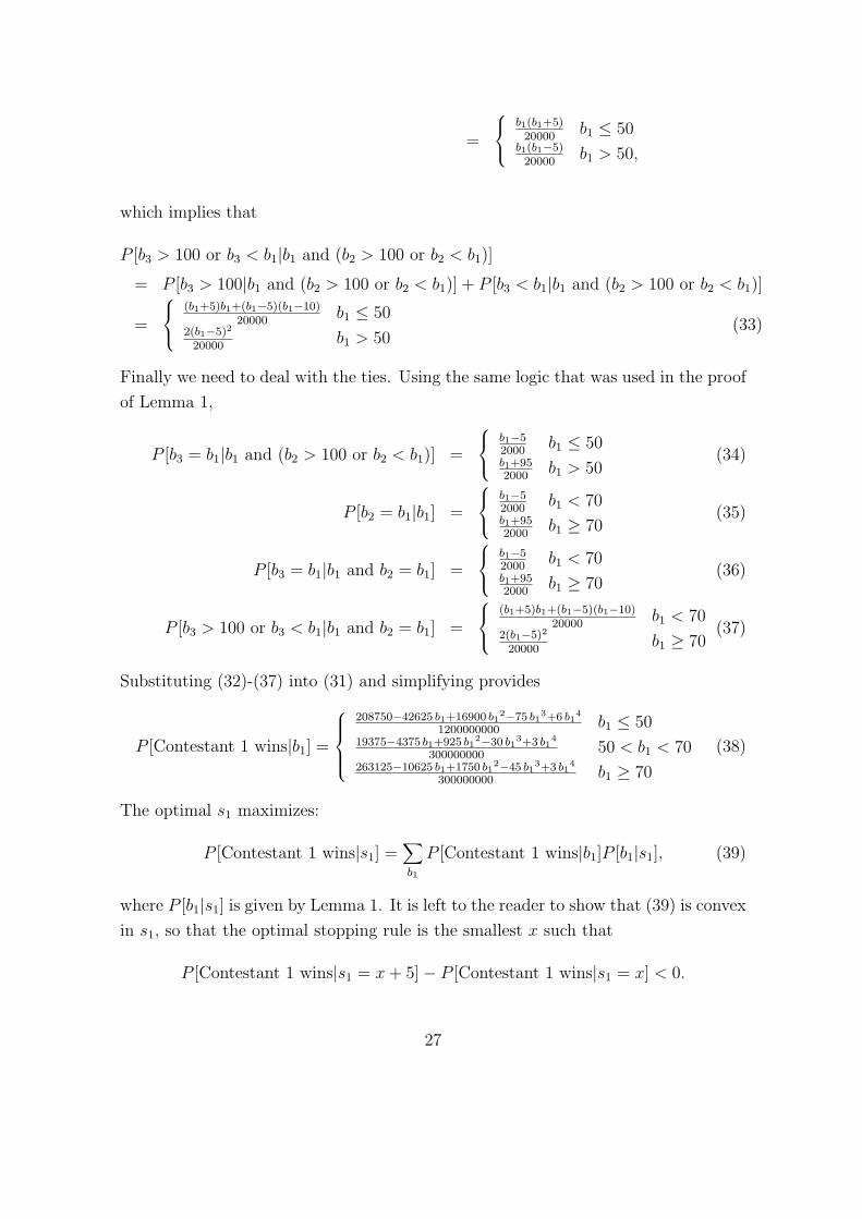
(33)
Finally we need to deal with the ties. Using the same logic that was used in the proof
of Lemma 1,
P [b3 = b1|b1 and (b2 > 100 or b2 < b1)] =
b1−52000
b1 ≤ 50b1+952000
b1 > 50(34)
P [b2 = b1|b1] =
b1−52000
b1 < 70b1+952000
b1 ≥ 70(35)
P [b3 = b1|b1 and b2 = b1] =
b1−52000
b1 < 70b1+952000
b1 ≥ 70(36)
P [b3 > 100 or b3 < b1|b1 and b2 = b1] =
(b1+5)b1+(b1−5)(b1−10)20000
b1 < 702(b1−5)2
20000b1 ≥ 70
(37)
Substituting (32)-(37) into (31) and simplifying provides
P [Contestant 1 wins|b1] =
208750−42625 b1+16900 b12−75 b1
3+6 b14
1200000000b1 ≤ 50
19375−4375 b1+925 b12−30 b1
3+3 b14
30000000050 < b1 < 70
263125−10625 b1+1750 b12−45 b1
3+3 b14
300000000b1 ≥ 70
(38)
The optimal s1 maximizes:
P [Contestant 1 wins|s1] =∑
b1
P [Contestant 1 wins|b1]P [b1|s1], (39)
where P [b1|s1] is given by Lemma 1. It is left to the reader to show that (39) is convex
in s1, so that the optimal stopping rule is the smallest x such that
P [Contestant 1 wins|s1 = x + 5]− P [Contestant 1 wins|s1 = x] < 0.
27

Evaluating this expression for x = 65 gives:
P [Contestant 1 wins|s1 = 70]− P [Contestant 1 wins|s1 = 65]
=20∑
i=14
263125− 10625 5i + 1750 (5i)2 − 45 (5i)3 + 3 (5i)4
300000000
(5
2000
)
−19375− 4375 (65) + 925 (65)2 − 30 (65)3 + 3 (65)4
300000000
(100
2000
)
=4613
6000000> 0.
Repeating this calculation for x = 70 gives:
P [Contestant 1 wins|s1 = 75]− P [Contestant 1 wins|s1 = 70]
=20∑
i=15
263125− 10625 5i + 1750 (5i)2 − 45 (5i)3 + 3 (5i)4
300000000
(5
2000
)
−263125− 10625 (70) + 1750 (70)2 − 45 (70)3 + 3 (70)4
300000000
(100
2000
)
= − 459347
192000000< 0.
So the optimal stopping rule is s1 = 70. •
28

References
Barberis, N, M. Huang and T Santos (2000), “Prospect Theory and Asset Prices,”
Working Paper.
Bennett, R.W. and K.A. Hickman (1993), Rationality and “The Price Is Right ”,
Journal of Economic Behavior and Organization, 21:99-105.
Berk, J., E. Hughson and K Vandezande (1996), The Price Is Right, but are the Bids?
An Investigation of Rational Decision Theory,American Economic Review, 86,
954-970.
Daniel, Kent, David Hirshleifer and Avanidhar Subrahmanyam (1998), “Investor Psy-
chology and Security Market Under- and Over-reactions,” Journal of Finance,
53(5) pp. 1839-1886.
Gervais, S and T. Odean, (2001), “”Learning to be Overconfident” with Simon Ger-
vais, Review of Financial Studies, 14:1-27.
McKelvey, R. D. and T. R. Palfrey (1992), An Experimental Study of the Centipede
Game, Econometrica, 60, 803–836.
Rabin, M. (1998), ”Psychology and Economics,” Journal of Economic Literature, Vol.
XXXVI, 11-46.
Rapoport, A., W. Stein, J. Parco, and T. Nicholas, (2001), Equilibrium Play and
Adaptive Learning in a Three-person Centipede Game, University of Arizona
working paper.
Tenorio, R, J. Baxidore, R. Battalio and T. Milbourn (1997), ”Analyzing Sequential
Game Equilibrium: A Natural Experiment from The Price Is Right ” (1997),
Working Paper, University of Notre Dame.
29