
Can 123 Variables Say Something About Inflation in … · Can 123 Variables Say Something About In...
49
Introduction Empirical estimations Results and conclusion Can 123 Variables Say Something About Inflation in Malaysia? Kue-Peng Chuah 1 Zul-fadzli Abu Bakar Preliminary work - please do no quote First version: January 2015 Current version: April 2017 TIAC - BNM Workshop Monetary Policy In Theory and Practice Session 2: Measuring Inflation Dynamics 23 May 2017 1 Presentation by Kue-Peng Chuah, [email protected] The opinions expressed in these slides and presentation are solely the responsibility of the authors and do not necessarily reflect the views of Bank Negara Malaysia. 1 / 31
-
Upload
truongdieu -
Category
Documents
-
view
221 -
download
7
Transcript of Can 123 Variables Say Something About Inflation in … · Can 123 Variables Say Something About In...
Introduction Empirical estimations Results and conclusion
Can 123 Variables Say SomethingAbout Inflation in Malaysia?
Kue-Peng Chuah1
Zul-fadzli Abu Bakar
Preliminary work - please do no quoteFirst version: January 2015
Current version: April 2017
TIAC - BNM WorkshopMonetary Policy In Theory and PracticeSession 2: Measuring Inflation Dynamics
23 May 2017
1Presentation by Kue-Peng Chuah, [email protected]
The opinions expressed in these slides and presentation are solely the responsibility of theauthors and do not necessarily reflect the views of Bank Negara Malaysia. 1 / 31

Introduction Empirical estimations Results and conclusion
Outline
1 IntroductionWhat we do in the paperContributionMotivation
2 Empirical estimationsDataMethodology
3 Results and conclusion
2 / 31

Introduction Empirical estimations Results and conclusion
Outline
1 IntroductionWhat we do in the paperContributionMotivation
2 Empirical estimationsDataMethodology
3 Results and conclusion
3 / 31
Introduction Empirical estimations Results and conclusion
What we do in the paper
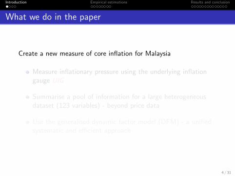
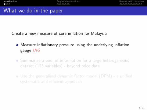
Create a new measure of core inflation for Malaysia
Measure inflationary pressure using the underlying inflationgauge UIG
Summarise a pool of information for a large heterogeneousdataset (123 variables) - beyond price data
Use the generalised dynamic factor model (DFM) - a unifiedsystematic and efficient approach
4 / 31
Introduction Empirical estimations Results and conclusion
What we do in the paper
Create a new measure of core inflation for Malaysia
Measure inflationary pressure using the underlying inflationgauge UIG
Summarise a pool of information for a large heterogeneousdataset (123 variables) - beyond price data
Use the generalised dynamic factor model (DFM) - a unifiedsystematic and efficient approach
4 / 31

Introduction Empirical estimations Results and conclusion
Contribution to the literature
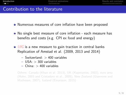
Numerous measures of core inflation have been proposed
No single best measure of core inflation - each measure hasbenefits and costs (e.g. CPI ex food and energy)
UIG is a new measure to gain traction in central banksReplication of Amstad et al. (2009, 2013 and 2014)
– Switzerland: > 400 variables– USA: > 300 variables– China: > 400 variables
Others: Canada (Khan et al. 2013), UK (Kapetanios, 2002), euro area(Hahn, 2003 and Cristadoro et al., 2005), New Zealand (Giannone andMatheson, 2007), Iceland (Einarsson, 2015)
5 / 31

Introduction Empirical estimations Results and conclusion
Contribution to the literature
Numerous measures of core inflation have been proposed
No single best measure of core inflation - each measure hasbenefits and costs (e.g. CPI ex food and energy)
UIG is a new measure to gain traction in central banksReplication of Amstad et al. (2009, 2013 and 2014)
– Switzerland: > 400 variables– USA: > 300 variables– China: > 400 variables
Others: Canada (Khan et al. 2013), UK (Kapetanios, 2002), euro area(Hahn, 2003 and Cristadoro et al., 2005), New Zealand (Giannone andMatheson, 2007), Iceland (Einarsson, 2015)
5 / 31
Introduction Empirical estimations Results and conclusion
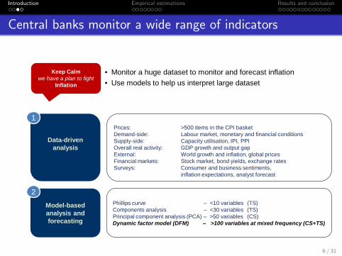
Central banks monitor a wide range of indicators
• Monitor a huge dataset to monitor and forecast inflation • Use models to help us interpret large dataset
Data-driven analysis
Model-based analysis and forecasting
Prices: >500 items in the CPI basket Demand-side: Labour market, monetary and financial conditions Supply-side: Capacity utilisation, IPI, PPI Overall real activity: GDP growth and output gap External: World growth and inflation, global prices Financial markets: Stock market, bond yields, exchange rates Surveys: Consumer and business sentiments, inflation expectations, analyst forecast
Phillips curve – <10 variables (TS) Components analysis – <30 variables (TS) Principal component analysis (PCA) – >50 variables (CS) Dynamic factor model (DFM) – >100 variables at mixed frequency (CS+TS)
1
2
Keep Calm we have a plan to fight
Inflation
6 / 31

Introduction Empirical estimations Results and conclusion
Measuring core inflation
Exclude volatile items
i.e. food and energy
Re-weight items in CPI
that are volatile or
price administered
Cross section (CS)
Univariate
• MA
• Trimmed mean
• Filters: HP,
band-pass, Kalman
Multivariate
• SVAR
• Kalman
Time series (TS)
Principal Component
Analysis (PCA)
Dynamic factor model
(DFM)
CS + TS
Smoothing / filtering
Common shortcoming :
consider a limited fraction of information or
a homogenous data set
Eliminate SR volatility
to smoothen
Eliminate idiosyncratic noise
and some volatility1 2 1 2
3
3
7 / 31

Introduction Empirical estimations Results and conclusion
Outline
1 IntroductionWhat we do in the paperContributionMotivation
2 Empirical estimationsDataMethodology
3 Results and conclusion
8 / 31

Introduction Empirical estimations Results and conclusion
Data
Balanced panel of monthly data from Jan. 2000 to Dec. 2014
𝒙𝟏 𝒙𝟐 𝒙𝟑 𝒙𝟏𝟐𝟑
𝒕 = 𝟏
𝒕 = 𝟐
𝒕 = 𝑻
Prices 54
Financial 15
Real activity 34
Money and credit 16
Labour 1
Prices Real activity
Labour Money
Financial International
International 3
Prices
Real activity
9 / 31
Introduction Empirical estimations Results and conclusion
Data
Broad and large dataset (nominal and real variables)
These relevant data are monitored for surveillance
Standardise each variable prior to estimation
10 / 31
Introduction Empirical estimations Results and conclusion
Data
Broad and large dataset (nominal and real variables)
These relevant data are monitored for surveillance
Standardise each variable prior to estimation
10 / 31
Introduction Empirical estimations Results and conclusion
Data
Broad and large dataset (nominal and real variables)
These relevant data are monitored for surveillance
Standardise each variable prior to estimation
10 / 31

Introduction Empirical estimations Results and conclusion
Methodology
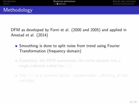
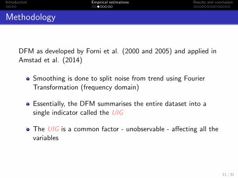
DFM as developed by Forni et al. (2000 and 2005) and applied inAmstad et al. (2014)
Smoothing is done to split noise from trend using FourierTransformation (frequency domain)
Essentially, the DFM summarises the entire dataset into asingle indicator called the UIG
The UIG is a common factor - unobservable - affecting all thevariables
11 / 31
Introduction Empirical estimations Results and conclusion
Methodology
DFM as developed by Forni et al. (2000 and 2005) and applied inAmstad et al. (2014)
Smoothing is done to split noise from trend using FourierTransformation (frequency domain)
Essentially, the DFM summarises the entire dataset into asingle indicator called the UIG
The UIG is a common factor - unobservable - affecting all thevariables
11 / 31
Introduction Empirical estimations Results and conclusion
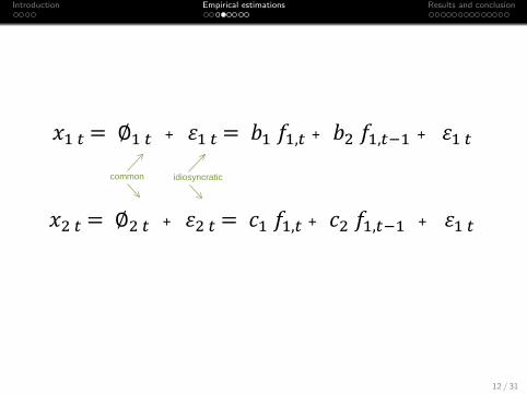
𝑥1 𝑡 = ∅1 𝑡 + 𝜀1 𝑡 = 𝑏1 𝑓1,𝑡 + 𝑏2 𝑓1,𝑡−1 + 𝜀1 𝑡
common idiosyncratic
𝑥2 𝑡 = ∅2 𝑡 + 𝜀2 𝑡 = 𝑐1 𝑓1,𝑡 + 𝑐2 𝑓1,𝑡−1 + 𝜀1 𝑡
12 / 31
Introduction Empirical estimations Results and conclusion
Methodology
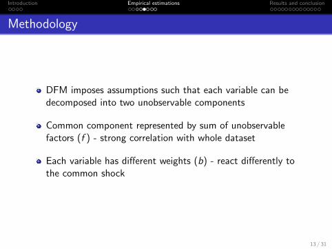
DFM imposes assumptions such that each variable can bedecomposed into two unobservable components
Common component represented by sum of unobservablefactors (f ) - strong correlation with whole dataset
Each variable has different weights (b) - react differently tothe common shock
13 / 31

Introduction Empirical estimations Results and conclusion
Methodology
Set frequency at [12 months] to capture shocks that persist(transitory vs. persistent shocks)
Set number of common factors at [two] - sufficiently reflectdataset, selection criteria using Bai and Ng (2008)
Set lag to [one] (distributed lag structure)
With new data release, DFM allocates a new set of weightswhen extracting underlying common factor to estimate theUIG
14 / 31

Introduction Empirical estimations Results and conclusion
inflation
signal
idiosyncratic
Unobserved Use all information in entire panel
UIG
Unobserved Noise
MR/LR
SR
15 / 31
Introduction Empirical estimations Results and conclusion
Benefits of DFM
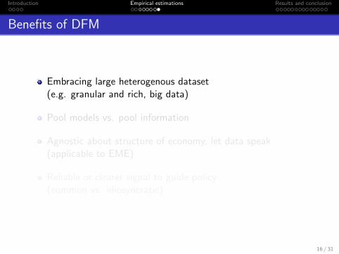
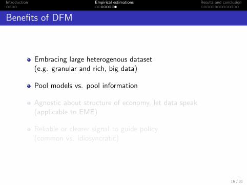
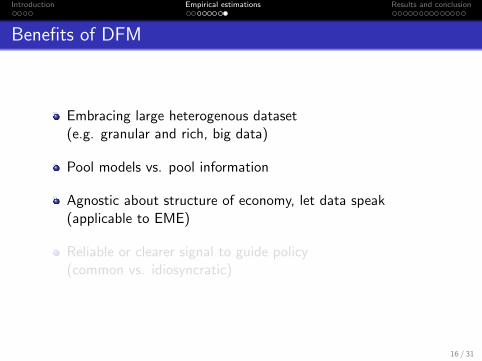
Embracing large heterogenous dataset(e.g. granular and rich, big data)
Pool models vs. pool information
Agnostic about structure of economy, let data speak(applicable to EME)
Reliable or clearer signal to guide policy(common vs. idiosyncratic)
16 / 31
Introduction Empirical estimations Results and conclusion
Benefits of DFM
Embracing large heterogenous dataset(e.g. granular and rich, big data)
Pool models vs. pool information
Agnostic about structure of economy, let data speak(applicable to EME)
Reliable or clearer signal to guide policy(common vs. idiosyncratic)
16 / 31

Introduction Empirical estimations Results and conclusion
Outline
1 IntroductionWhat we do in the paperContributionMotivation
2 Empirical estimationsDataMethodology
3 Results and conclusion
17 / 31

Introduction Empirical estimations Results and conclusion
-4
-2
0
2
4
6
8
10
Mar
-01
Aug-
01Ja
n-02
Jun-
02N
ov-0
2Ap
r-03
Sep-
03Fe
b-04
Jul-0
4D
ec-0
4M
ay-0
5O
ct-0
5M
ar-0
6Au
g-06
Jan-
07Ju
n-07
Nov
-07
Apr-0
8Se
p-08
Feb-
09Ju
l-09
Dec
-09
May
-10
Oct
-10
Mar
-11
Aug-
11Ja
n-12
Jun-
12N
ov-1
2Ap
r-13
Sep-
13Fe
b-14
Jul-1
4
UIG vs. Headline Inflation 2001: 2014
UIG Headline
Y-o-Y growth, %
18 / 31

Introduction Empirical estimations Results and conclusion
-2
-1
0
1
2
3
4
5
6
7
8
Mar
-01
Aug-
01Ja
n-02
Jun-
02N
ov-0
2Ap
r-03
Sep-
03Fe
b-04
Jul-0
4D
ec-0
4M
ay-0
5O
ct-0
5M
ar-0
6Au
g-06
Jan-
07Ju
n-07
Nov
-07
Apr-0
8Se
p-08
Feb-
09Ju
l-09
Dec
-09
May
-10
Oct
-10
Mar
-11
Aug-
11Ja
n-12
Jun-
12N
ov-1
2Ap
r-13
Sep-
13Fe
b-14
Jul-1
4
UIG vs. Core (exclusion) Inflation 2001:2014
UIG Core
Y-o-Y growth, %
19 / 31

Introduction Empirical estimations Results and conclusion
-2
-1
0
1
2
3
4
5
6
7
8
Mar
-01
Aug-
01Ja
n-02
Jun-
02N
ov-0
2Ap
r-03
Sep-
03Fe
b-04
Jul-0
4D
ec-0
4M
ay-0
5O
ct-0
5M
ar-0
6Au
g-06
Jan-
07Ju
n-07
Nov
-07
Apr-0
8Se
p-08
Feb-
09Ju
l-09
Dec
-09
May
-10
Oct
-10
Mar
-11
Aug-
11Ja
n-12
Jun-
12N
ov-1
2Ap
r-13
Sep-
13Fe
b-14
Jul-1
4
UIG vs. PCA 2001: 2014
UIG PCA
Y-o-Y growth, %
20 / 31
Introduction Empirical estimations Results and conclusion
-2
-1
0
1
2
3
4
5
6
7
8
Mar
-01
Aug-
01Ja
n-02
Jun-
02N
ov-0
2Ap
r-03
Sep-
03Fe
b-04
Jul-0
4D
ec-0
4M
ay-0
5O
ct-0
5M
ar-0
6Au
g-06
Jan-
07Ju
n-07
Nov
-07
Apr-0
8Se
p-08
Feb-
09Ju
l-09
Dec
-09
May
-10
Oct
-10
Mar
-11
Aug-
11Ja
n-12
Jun-
12N
ov-1
2Ap
r-13
Sep-
13Fe
b-14
Jul-1
4
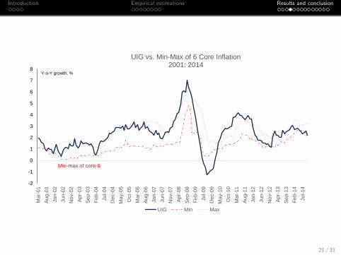
UIG vs. Min-Max of 6 Core Inflation 2001: 2014
UIG Min Max
Y-o-Y growth, %
Min-max of core-6
21 / 31

Introduction Empirical estimations Results and conclusion
-4
-2
0
2
4
6
8
10
Mar
-01
Aug-
01Ja
n-02
Jun-
02N
ov-0
2Ap
r-03
Sep-
03Fe
b-04
Jul-0
4D
ec-0
4M
ay-0
5O
ct-0
5M
ar-0
6Au
g-06
Jan-
07Ju
n-07
Nov
-07
Apr-0
8Se
p-08
Feb-
09Ju
l-09
Dec
-09
May
-10
Oct
-10
Mar
-11
Aug-
11Ja
n-12
Jun-
12N
ov-1
2Ap
r-13
Sep-
13Fe
b-14
Jul-1
4
UIG vs. Headline vs. Core Inflation
UIG Core Headline
UIG (1.38)
PCA (1.31)
Core (1.01)
Core-6 (0.97)
Headline (1.59)
UIG --
PCA 0.78 --
Core 0.74 0.93 --
Core-6 0.79 0.96 0.97
Headline 0.87 0.72 0.71 0.78
Y-o-Y growth, %
22 / 31
Introduction Empirical estimations Results and conclusion
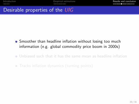
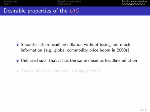
Desirable properties of the UIG
Smoother than headline inflation without losing too muchinformation (e.g. global commodity price boom in 2000s)
Unbiased such that it has the same mean as headline inflation
Tracks inflation dynamics (turning points)
23 / 31
Introduction Empirical estimations Results and conclusion
Desirable properties of the UIG
Smoother than headline inflation without losing too muchinformation (e.g. global commodity price boom in 2000s)
Unbiased such that it has the same mean as headline inflation
Tracks inflation dynamics (turning points)
23 / 31

Introduction Empirical estimations Results and conclusion
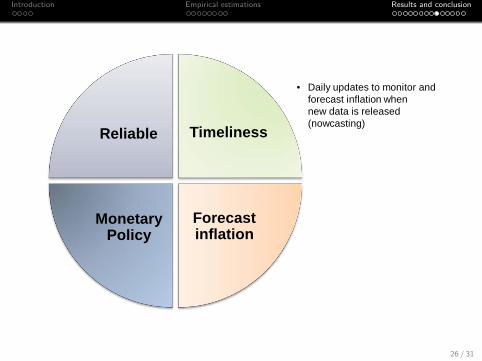
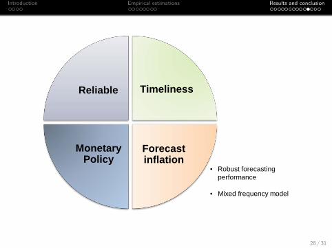
Why the UIG is useful
Reliable Timeliness
Forecast inflation
Monetary Policy
24 / 31

Introduction Empirical estimations Results and conclusion
Reliable Timeliness
Forecast inflation
Monetary Policy
• More reliable signal of turning points
• Headline too volatile, core tends to ignore a lot of information
• Use information across variables and time (CS and TS)
25 / 31
Introduction Empirical estimations Results and conclusion
Reliable Timeliness
Forecast inflation
Monetary Policy
• Daily updates to monitor and forecast inflation when new data is released (nowcasting)
26 / 31

Introduction Empirical estimations Results and conclusion
Reliable Timeliness
Forecast inflation
Monetary Policy
• MP transmission has long, variable and uncertain lags, should not react to noise or idiosyncratic effects
• Exclude information not related to policymakers’ decision-making time horizon
27 / 31
Introduction Empirical estimations Results and conclusion
Reliable Timeliness
Forecast inflation
Monetary Policy
• Robust forecasting performance
• Mixed frequency model
28 / 31

Introduction Empirical estimations Results and conclusion
Conclusion (last slide!)
UIG contains desirable properties as a measure of coreinflation - promising preliminary results
UIG can be developed further as a regular feature tocomplement inflation toolkit of policymakers
Future work on UIG
– Expansion of dataset (300 variables)– Robustness analysis– Forecasting performance (horse race)
29 / 31

Introduction Empirical estimations Results and conclusion
Thank you
Comments welcome
30 / 31

Introduction Empirical estimations Results and conclusion
References
Amstad, M. and Huan, Y. and Ma, G. (2014). Developing an underlying inflation gauge for China. BIS WorkingPaper No. 465.
Bai, J. and Ng, S. (2002). Determining the number of factors in approximate factor models. Econometrica.
Bank Negara Malaysia (2008). Core inflation: measurements and evaluation. Bank Negara Malaysia AnnualReport, Chapter 3.
Bernanke, B., and Boivin, J. (2003). Monetary policy in a data-rich environment. Journal of Monetary Economics.
Chuah, K., Chong, E., and Tan, J. (2015). Global commodity prices and inflation dynamics in Malaysia. BankNegara Malaysia Working Paper No. 5/2015.
Forni, M., Hallin, M., Lippi, M. and Reichlin, L. (2000). The generalized dynamic-factor model: identification andestimation. Review of Economics and Statistics.
Forni, M., Hallin, M., Lippi, M., and Reichlin, L. (2005). The generalized dynamic factor model. Journal of theAmerican Statistical Association.
Hahn, E. (2002). Core inflation in the Euro Area: an application of the generalized dynamic factor model. Centerfor Financial Studies Working Paper No. 2002/11.
Kozicki, S. (2001). Why do central banks monitor so many inflation indicators?. Economic Review Federal ReserveBank of Kansas City.
31 / 31