Cams Design

MACHINE THEORY

Bachelor in Mechanical Engineering

CAMS DESIGN

Ignacio Valiente BlancoJosé Luis Pérez DíazDavid Mauricio Alba LuceroEfrén Díez Jiménez

INDEX

� 1. Introduction

� 2. Cams clasification

� 3. Desmodromic Cams

� 4. Followers clasification

� 5. Closure Joints clasification

� 6. Classification of Cams mechanisms

� 7. SVAJ Diagrams

� 8. Fundamental Law of Cams

► 8.1 Simple Harmonic Motion

► 8.2 Polynomial Functions

► 8.3 Functions Comparison

� 9. What can cams do?

� Literature 2

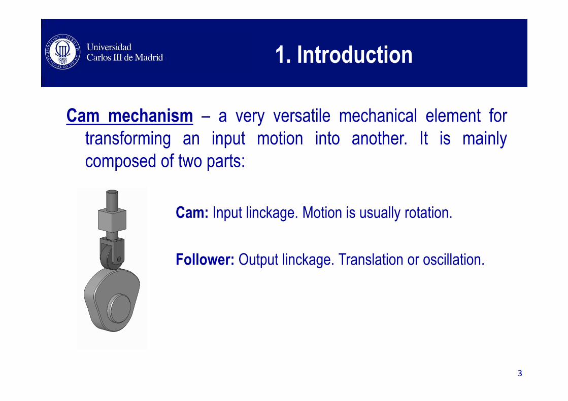
1. Introduction

Cam mechanism – a very versatile mechanical element for

transforming an input motion into another. It is mainly

composed of two parts:

Cam: Input linckage. Motion is usually rotation.

Follower: Output linckage. Translation or oscillation.

3

1. Introduction

� Advantages of cams

• Many possibilities of motion transformation. Very versatile.

• Have few parts.

• Take small space.

• Widely used in industry. Known technology.

� Limitations of cams

• Suceptible to vibrations.

• Wear.

• Fatigue.

• Lubrication needed.

4

1. Introduction

� Cams are usually classified according to the cam geometry:

► Planar cams

� Disc or plate cams

� Linear cams: Cam do not rotate. Backwards and forwards motion.

5

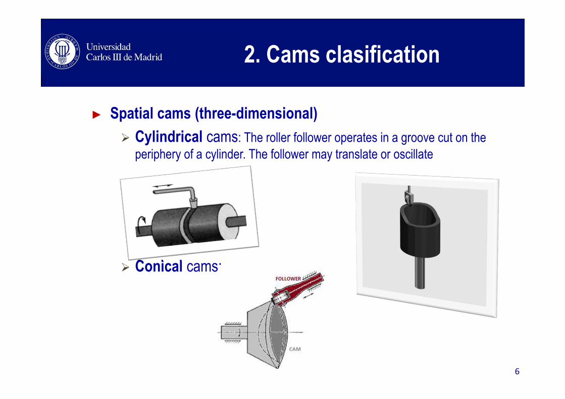
2. Cams clasification

► Spatial cams (three-dimensional)

� Cylindrical cams: The roller follower operates in a groove cut on the

periphery of a cylinder. The follower may translate or oscillate

� Conical cams:

6


7

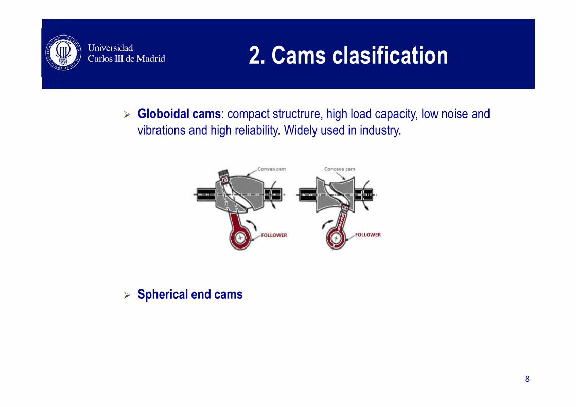
� Globoidal cams: compact structrure, high load capacity, low noise and

vibrations and high reliability. Widely used in industry.

� Spherical end cams


8

� Cams can be classified according to the follower motion respect

the rotation axle of the cam

► Radial Cams

► Translational or Axial Cams


9

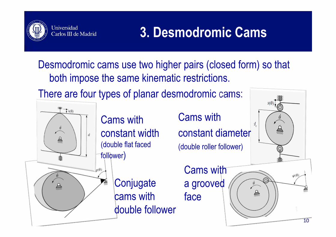
Desmodromic cams use two higher pairs (closed form) so that

both impose the same kinematic restrictions.

There are four types of planar desmodromic cams:

3. Desmodromic Cams

Cams with

constant width(double flat faced

follower)

Cams with

constant diameter(double roller follower)

Conjugate

cams with

double follower

Cams with

a grooved

face

10

4. Followers clasification

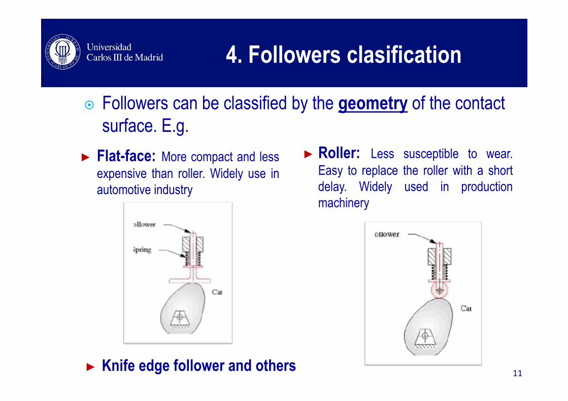
► Roller: Less susceptible to wear.

Easy to replace the roller with a short

delay. Widely used in production

machinery

► Flat-face: More compact and less

expensive than roller. Widely use in

automotive industry

� Followers can be classified by the geometry of the contact

surface. E.g.

► Knife edge follower and others11

4. Followers clasification

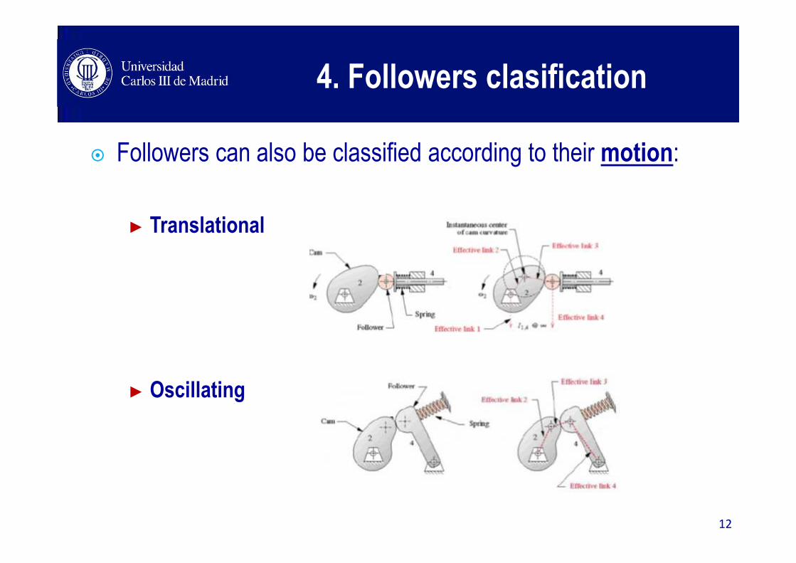
� Followers can also be classified according to their motion:

► Translational

► Oscillating

12

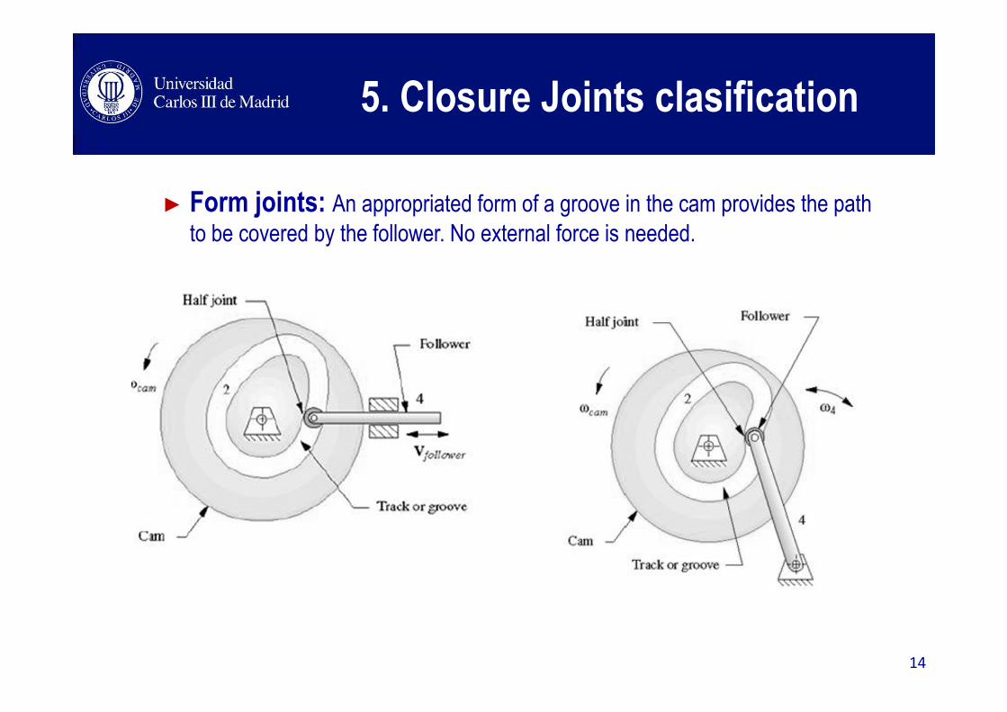
5. Closure Joints clasification

� Joint closure between the cam and the follower is an important point to

take into account when design a cam mechanism. It is a high kinematic

pair (See Introduction to kinematics and mechanisms)

► Force Joints: An external force assure permanent contact between the follower

and the cam surface. Springs, gravity and inertial systems.

13

5. Closure Joints clasification

► Form joints: An appropriated form of a groove in the cam provides the path

to be covered by the follower. No external force is needed.

14

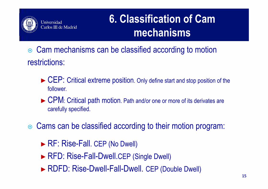
6. Classification of Cam

mechanisms

� Cam mechanisms can be classified according to motion

restrictions:

►CEP: Critical extreme position. Only define start and stop position of the

follower.

►CPM: Critical path motion. Path and/or one or more of its derivates are

carefully specified.

� Cams can be classified according to their motion program:

►RF: Rise-Fall. CEP (No Dwell)

►RFD: Rise-Fall-Dwell.CEP (Single Dwell)

►RDFD: Rise-Dwell-Fall-Dwell. CEP (Double Dwell)1515

• The first step when design cam is to define the mathematical

functions to be used to define the motion of the follower.

• SVAJ diagrams are a useful tool:

S: displacement of the follower vs θ of the cam. s

V: velocity. ∂s/ ∂t

A: acceleration. ∂2s/ ∂t2

J: Jerk. (golpe) ∂3s/ ∂t3

7. SVAJ Diagrams

16

• E.g.:

• A cam mechanism will be designed for a

driller machine.

• Operation conditions:

- One part each 20s. Initial position: A

- DRILL IN: 25 mm in 5 s. B-C

- DWELL: 5 s finishing the drill.C-D

- DRILL OUT: 25 mm in 5s.D-A

- DWELL: Wait for another part.A-B 5s

DWELL

B-CA-B

C-D D-A

VdrillInput part

¿? QUESTION ¿? What is the motion program? How many dwells are there?

-

7. SVAJ Diagrams

17

• E.g.:

• A cam mechanism will be designed for a

driller machine.

• Operation conditions:

- One part each 20s. Initial position: A

- DRILL IN: 25 mm in 5 s. B-C

- DWELL: 5 s finishing the drill.C-D

- DRILL OUT: 25 mm in 5s.D-A

- DWELL: Wait for another part.A-B 5s

DWELL

B-CA-B

C-D D-A

VdrillInput part

¿? QUESTION ¿? What is the motion program? How many dwells are there?

RDFD: Rise-Dwell-Fall-Dwell. 2Dwells

-

7. SVAJ Diagrams

18

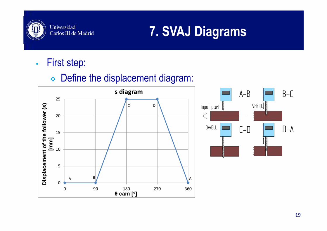
• First step:

� Define the displacement diagram:

0

5

10

15

20

25

0 90 180 270 360

Dis

plac

emen

t of t

he fo

llow

er (s

) [m

m]

θ cam [º]

s diagram

A B

C D

A

DWELL

B-CA-B

C-D D-A

VdrillInput part

7. SVAJ Diagrams

19

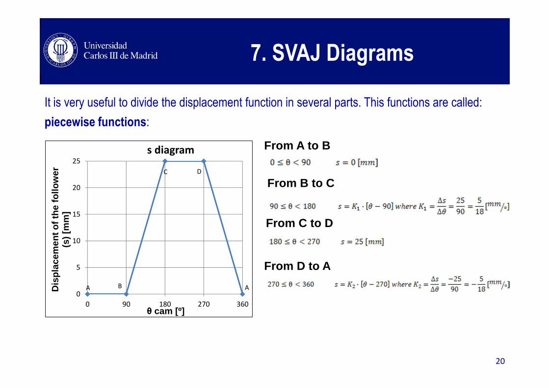
It is very useful to divide the displacement function in several parts. This functions are called:

piecewise functions:

0

5

10

15

20

25

0 90 180 270 360

Dis

plac

emen

t of t

he fo

llow

er

(s)

[mm

]

θ cam [º]

s diagram

A B

C D

A

From D to A

From C to D

From B to C

From A to B

7. SVAJ Diagrams

20

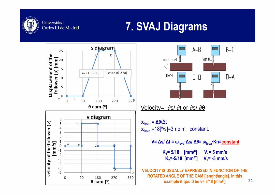
DWELL

B-CA-B

C-D D-A

VdrillInput part

Velocity= ∂s/ ∂t or ∂s/ ∂θ

ωleva = ∆θ/∆t

ωleva =18[º/s]=3 r.p.m constant.

V= ∆s/ ∆t = ωleva�∆s/ ∆θ= ωleva�Kn=constant

K1= 5/18 [mm/º] V1= 5 mm/s

K2=-5/18 [mm/º] V2= -5 mm/s

VELOCITY IS USUALLY EXPRESSED IN FUNCTION OF THE

ROTATED ANGLE OF THE CAM [lenght/angle]. In this

example it qould be v= 5/18 [mm/º]

7. SVAJ Diagrams

21

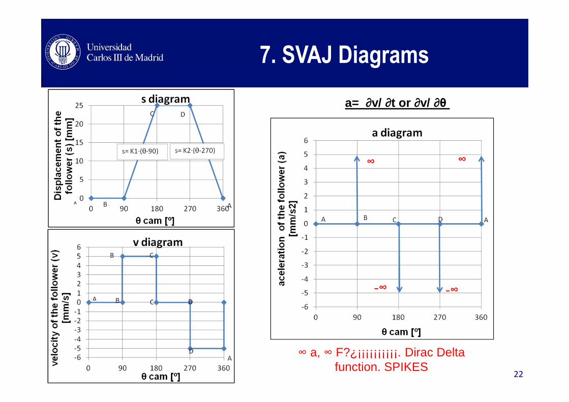
∞ a, ∞ F?¿¡¡¡¡¡¡¡¡¡¡. Dirac Delta function. SPIKES

a= ∂v/ ∂t or ∂v/ ∂θ

7. SVAJ Diagrams

22

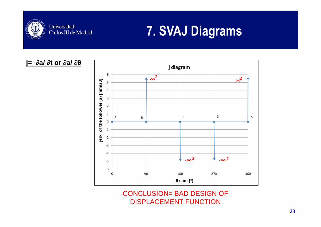
7. SVAJ Diagrams

CONCLUSION= BAD DESIGN OF DISPLACEMENT FUNCTION

j= ∂a/ ∂t or ∂a/ ∂θ

23

8. Fundamental Law of Cams

Design

SOME CONSIDERATIONS

1. In any but the simplest of cams, the cam motion program cannot be defined by a single

mathematical expression, but rather must be defined by several separate functions, each

of which defines the follower behavior over one segment, or piece, of the cam. These

expressions are sometimes called piecewise functions.2. These functions must have third-order continuity (the function plus two derivatives) at all

boundaries.

3. The displacement, velocity and acceleration functions must have no discontinuities in

them.

1. “The cam function must be continuous through the first and second

derivatives of displacement across the entire interval”

2. “The jerk function must be finite across the entire interval”

24

The example analyzed before does not comply with the fundamental law of cam design¡¡¡¡

DWELL

B-CA-B

C-D D-A

VdrillInput part

8. Fundamental Law of Cams

Design

25

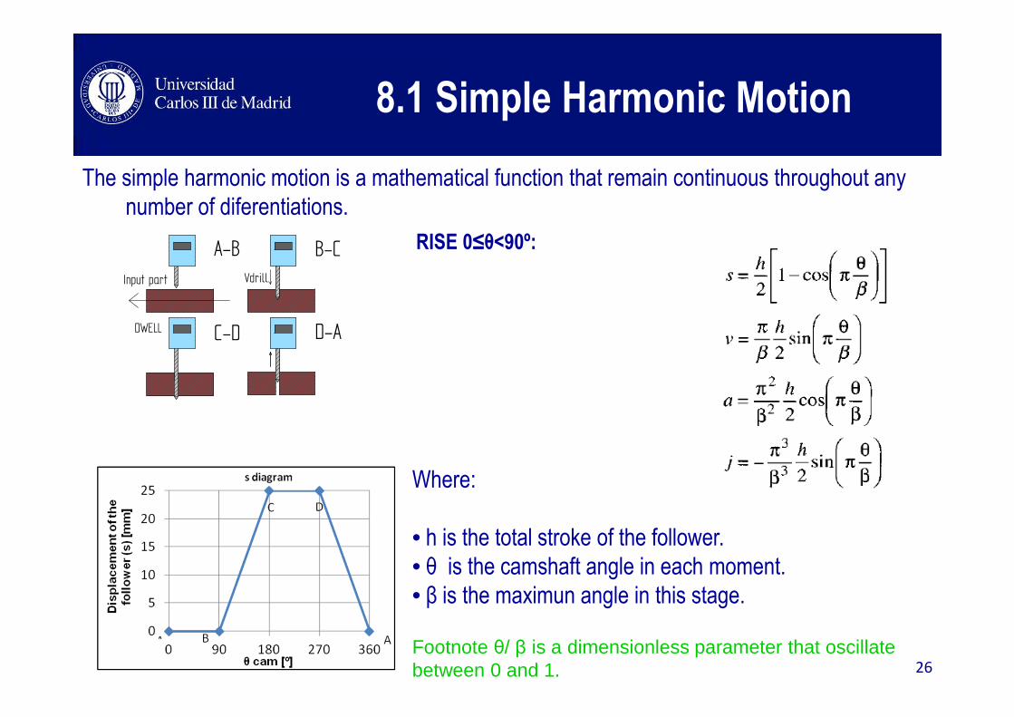
8.1 Simple Harmonic Motion

DWELL

B-CA-B

C-D D-A

VdrillInput part

The simple harmonic motion is a mathematical function that remain continuous throughout any

number of diferentiations.

Where:

• h is the total stroke of the follower.

• θ is the camshaft angle in each moment.

• β is the maximun angle in this stage.

Footnote θ/ β is a dimensionless parameter that oscillatebetween 0 and 1.

RISE 0≤θ<90º:

26

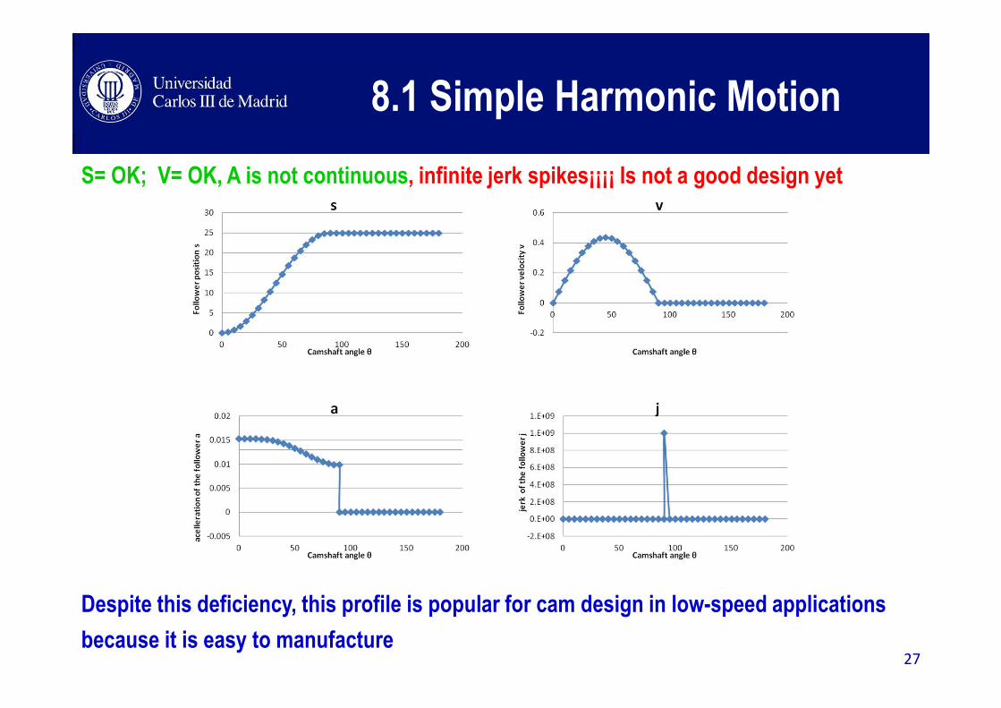
S= OK; V= OK, A is not continuous, infinite jerk spikes¡¡¡¡ Is not a good design yet

Despite this deficiency, this profile is popular for cam design in low-speed applications

because it is easy to manufacture

8.1 Simple Harmonic Motion

27

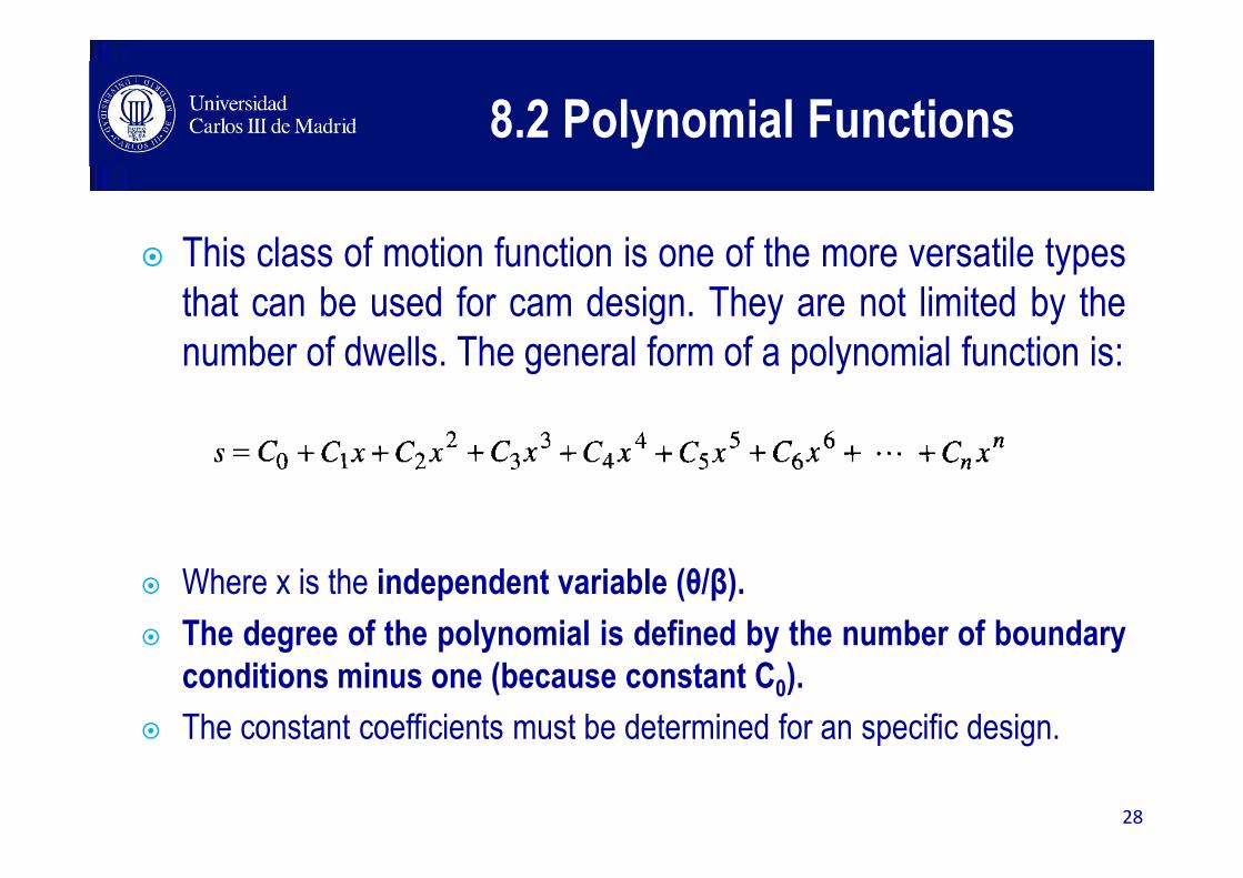
� This class of motion function is one of the more versatile types

that can be used for cam design. They are not limited by the

number of dwells. The general form of a polynomial function is:

� Where x is the independent variable (θ/β).

� The degree of the polynomial is defined by the number of boundary

conditions minus one (because constant C0).

� The constant coefficients must be determined for an specific design.

8.2 Polynomial Functions

28

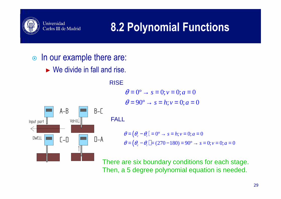
� In our example there are:

► We divide in fall and rise.

0º 0; 0; 0

90º ; 0; 0

s v a

s h v a

θθ

= → = = == → = = =

DWELL

B-CA-B

C-D D-A

VdrillInput part

RISE

( )( )

0º ; 0; 0

(270 180) 90º 0; 0; 0

c i

c i

s h v a

s v a

θ θ θθ θ θ

= − = → = = =

= − = − = → = = =

FALL

There are six boundary conditions for each stage.Then, a 5 degree polynomial equation is needed.


29

2 3 4 5

1 2 3 4 5

2 3 4

1 2 3 4 5

2 3

2 3 4 52

3 43

12 3 4 5

12 6 12 20

16 24

s Co C C C C C

v C C C C C

a C C C C

j C C

θ θ θ θ θβ β β β β

θ θ θ θβ β β β β

θ θ θβ β β β

θβ β

= + + + + +

= + + + +

= + + +

= + +

2

560Cθβ

Constant Condition Evaluation

C0 θ0; s=h h

C1 θ0; v=0 0

C2 θ0; a=0 0

C3 θ90; eq. 10h =250

C4 θ90; eq. -15h =-375

C5 θ90; eq. 6h=150

RISE

3 4 5

3 4 5 3 4 5

3 4 5

0

0 3 4 5 10 ; 15 ; 6

0 6 12 20

s C C C

v C C C C h C h C h

a C C C

θ βθ βθ β

= → = = + += → = = + + = = − == → = = + +

→→→→

0º 0; 0; 0

90º ; 0; 0

s v a

s h v a

θθ

= → = = == → = = =


30

2 3 4 5

1 2 3 4 5

2 3 4

1 2 3 4 5

2 3

2 3 4 52

3 43

12 3 4 5

12 6 12 20

16 24

s Co C C C C C

v C C C C C

a C C C C

j C C



θ θ θβ β β β

θβ β

= + + + + +

= + + + +

= + + +

= + +

2

560Cθβ


C0 θ0; s=h h

C1 θ0; v=0 0

C2 θ0; a=0 0

C3 θ90; eq. 10h =250

C4 θ90; eq. -15h =-375

C5 θ90; eq. 6h=150

RISE0º 0; 0; 0

90º ; 0; 0

s v a

s h v a

θθ

= → = = == → = = =

THIS POLYNOMIAL FUNCTION IS CALLED 3-4-5 POLYNOMIAL MOTION.


31

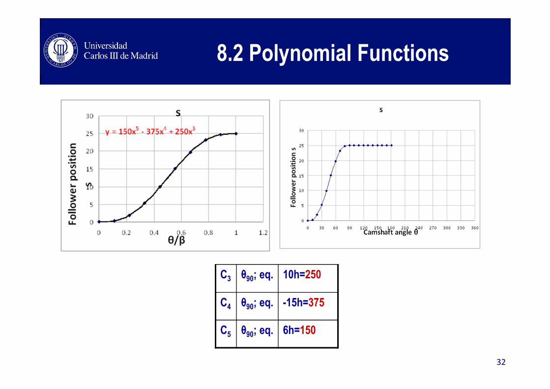
C3 θ90; eq. 10h=250

C4 θ90; eq. -15h=375

C5 θ90; eq. 6h=150


32

2 3 4 5

1 2 3 4 5

2 3 4

1 2 3 4 5

2 3

2 3 4 52

3 43

12 3 4 5

12 6 12 20

16 24

s Co C C C C C

v C C C C C

a C C C C

j C C



θ θ θβ β β β

θβ β

= + + + + +

= + + + +

= + + +

= + +

2

560Cθβ


C0 θ0; s=h h

C1 θ0; v=0 0

C2 θ0; a=0 0

C3 θ90; eq. -10h =-250

C4 θ90; eq. 15h =375

C5 θ90; eq. -6h=-150

FALL

3 4 5

3 4 5 3 4 5

3 4 5

0

0 3 4 5 10 ; 15 ; 6

0 6 12 20

s h C C C

v C C C C h C h C h

a C C C

θ βθ βθ β

= → = = + + += → = = + + = − = = −= → = = + +

→→→→

( )( )

0º ; 0; 0

(270 180) 90º 0; 0; 0

c i

c i

s h v a

s v a

θ θ θθ θ θ

= − = → = = =

= − = − = → = = =

Footnote: Please notice that C factors are the opposite to the RISE stage


33

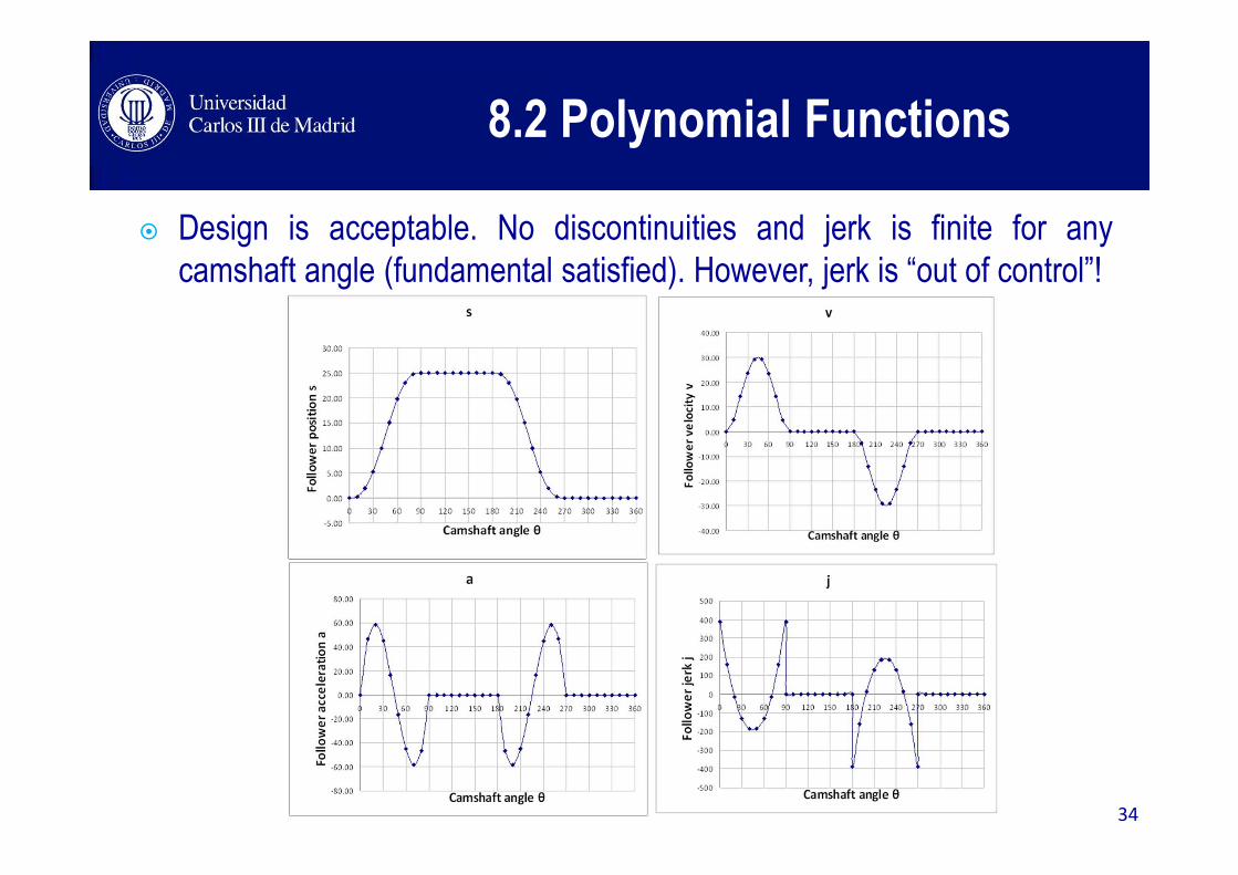
� Design is acceptable. No discontinuities and jerk is finite for any

camshaft angle (fundamental satisfied). However, jerk is “out of control”!


34

� The 4-5-6-7 POLYNOMIAL MOTION

► We can control jerk by adding two more restrictions and therefore

avoid the initial jerk (θ=0º;j>0) which could be harmful:

0º 0; 0; 0;

90º ; 0; 0;

0

0

s v a

s h v a

j

j

θθ

= → = = == → = = =

==

( )( )

0º ; 0; 0; 0

(270 180) 90º 0; 0; 0; 0

c i

c i

s h v a

s

j

v ja

θ θ θθ θ θ

= − = → = = =

= − = − = → = = =

=

=

Rise

Fall


35

2 3 4 5 6 7

1 2 3 4 5 6 7

2 3 4 5 6

1 2 3 4 5 6 7

2 3 42

12 3 4 5 6 7

12 6 12

s Co C C C C C C C

v C C C C C C C

a C C C

θ θ θ θ θ θ θβ β β β β β β

θ θ θ θ θ θβ β β β β β β

θ θβ β β

= + + + + + + +

= + + + + + +

= + +

2 3 4 5

5 6 7

2 3 4

3 4 5 6 73

20 30 42

16 24 60 120 210

C C C

j C C C C C

θ θ θβ β β


+ + +

= + + + +

POLYNOMIAL 4-5-6-7 JERK CONTROL

4 5 6 7

4 5 6 7

4 5 6 7

4 5 6 7

0

0 4 5 6 7

0 12 20 30 42

0 24 60 120 210

s C C C C

v C C C C

a C C C C

j C C C C

θ βθ βθ βθ β

= → = = + + += → = = + + += → = = + + += → = = + + +


C0 θ0; s=0 0

C1 θ0; v=0 0

C2 θ0; a=0 0

C3 θ0; j=0 0

C4 θ90; eq. -35h

C5 θ90; eq. -84h

C6 θ90; eq. 70h

C7 θ90; eq. -20h


36

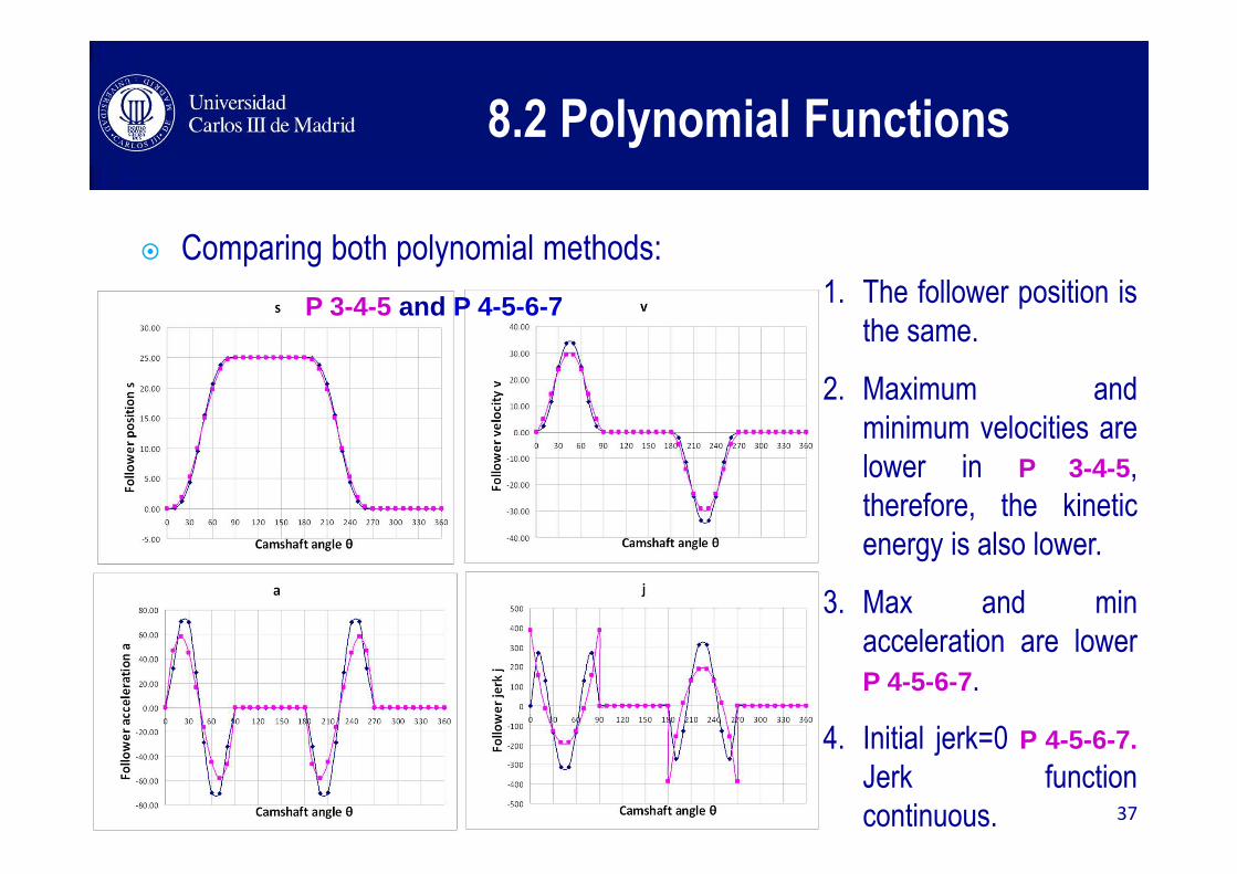
� Comparing both polynomial methods:

1. The follower position is

the same.

2. Maximum and

minimum velocities are

lower in P 3-4-5,

therefore, the kinetic

energy is also lower.

3. Max and min

acceleration are lower

P 4-5-6-7.

4. Initial jerk=0 P 4-5-6-7.Jerk function

continuous.

P 3-4-5 and P 4-5-6-7


37

� There are many other motion functions which can be used

(see literature).

► The best function motion will depend on the concrete application:

� Single Dwell

� Double Dwell

� Low-speed applications

� High-speed applications

� Displacement, velocity or acceleration specifications.

� Some examples are: cycloidal displacement, modified trapezoidal

accelerations, modified sinusoidal acceleration….


38

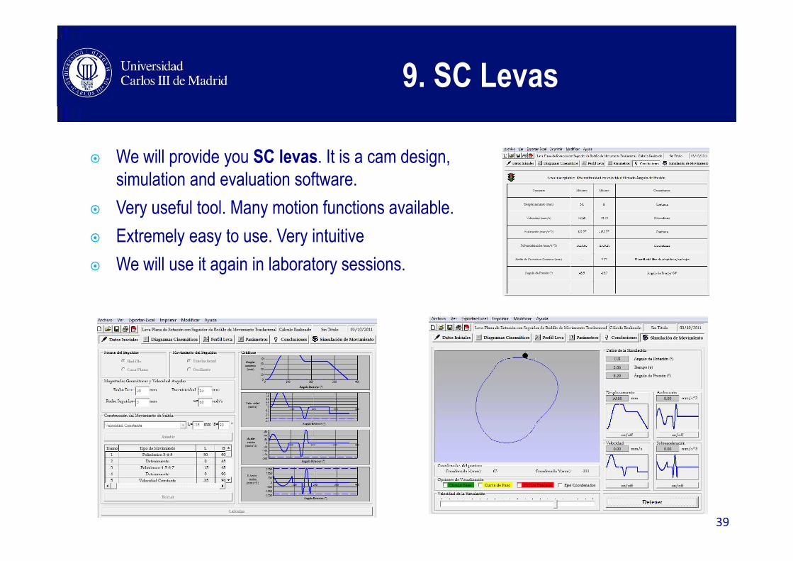
� We will provide you SC levas. It is a cam design,

simulation and evaluation software.

� Very useful tool. Many motion functions available.

� Extremely easy to use. Very intuitive

� We will use it again in laboratory sessions.

9. SC Levas

39

10 What can do cams?

40

http://www.youtube.com/watch?v=2Ah9Mhd6CRA

http://www.youtube.com/watch?v=ykx1DettTDM

http://www.youtube.com/watch?v=ocfIYUc5bpU

http://www.youtube.com/watch?v=ttZJQldd6qM

http://www.youtube.com/watch?v=ESRsd1TeOSg&feature=related

http://www.youtube.com/watch?v=MgklyL0wkVM

http://www.youtube.com/watch?v=0dDiXJsmDOQ

Literature

� Erdman, A.G., Sandor, G.N. and Sridar Kota Mechanism Design. Prentice Hall,

2001. Fourth Edition.

� Robert L. Norton. Design of Machinery. Ed.Mc Graw Hill 1995. Second Edition

� Shigley, J.E. & Uicker, J.J. Teoría de máquinas y mecanismos. McGraw-Hill, 1998

� SOFTWARE► SC levas

� VIDEOS

► http://www.youtube.com/watch?v=2Ah9Mhd6CRA

► http://www.youtube.com/watch?v=ykx1DettTDM

► http://www.youtube.com/watch?v=ocfIYUc5bpU

► http://www.youtube.com/watch?v=ttZJQldd6qM

► http://www.youtube.com/watch?v=ESRsd1TeOSg&feature=related

► http://www.youtube.com/watch?v=MgklyL0wkVM

► http://www.youtube.com/watch?v=0dDiXJsmDOQ41

Cams Design

Documents

Transcript of Cams Design