CALIFORNIA'S SERPENTINE

by Art Kruckeberg

Serpentine Rock

Californians boast of their world-class tallest and oldest trees, highest mountain and deepest valley; but that "book of records" can claim another first for the state. California, a state with the richest geological tapestry on the continent, also has the largest exposures of serpentine rock in North America. Indeed, this unique and colorful rock, so abundantly distributed around the state, is California's state rock. For botanists, the most dramatic attribute of serpentine is its highly selective, demanding influence on plant life. The unique flora growing on serpentine in California illustrates the ecological truism that though regional climate controls overall plant distribution, regional geology controls local plant diversity. Geology is used here in its broad sense to include land forms, rocks and soils.

Geologists of the early days in California were aware of serpentine to a greater extent than the early botanists. An 1826 geological map of San Francisco Bay area plots serpentine outcrops. The map, a work of naturalists with the H.M.S. Blossom, located serpentine on Tiburon Peninsula and Angel Island. The first major geological survey of California by Whitney in 1865 recorded serpentine too; yet the survey failed to connect serpentine with the barren-ness of the vast landscape in their visit to New Idria in San Benito County, the most spectacular serpentine occurrence in the state. As the state began to extract mineral resources, serpentine became more widely recognized. Mercury, chromium, nickel, asbestos and magnesite were found in or adjacent to serpentine out-crops. In a 1918 report on quicksilver (mercury ore) deposits of the state, a photo of the New Idria land-scape is captioned: "Serpentine surface near New Idria . . . showing characteristic sparseness of timber and brush growth."

Serpentine rock was named for the likeness of the rock to the mottled pattern of a snake's skin. In Greek, the word "serpent" translates to ophidion, from which the species name is derived for the serpentine endemic grass, Calamagrostis ophitidis. The Greek physician Dioscorides apparently recommended ground serpen-tine rock for the prevention of snake bite, surely a rather extreme remedy. The word, serpentine, has come to be used both for the rock and for the soils derived from the rock.

Traditional teaching in geology tells us that rocks can be divided into three major categories—igneous, metamorphic, and sedimentary. The igneous rocks, formed by cooling from molten rock called magma, are broadly classified as mafic or silicic depending mainly on the amount of magnesium and iron or silica present. Serpentine is called an ultramafic rock because of the presence of unusually large amounts of magnesium and iron. Igneous rocks, particularly those that originate within the earth's crust, above the mantle, contain small but significant amounts of

Views of the classic serpentine areas at New Idria in San Benito County. The upper photo was taken in 1932, the lower in 1960 of the same view; no evident change in 28 years. Photos courtesy of the U.S. Forest Service and Dr. James Griffin.

ORANGE

calcium, sodium, and potassium, along with small amounts of iron and magnesium. Serpentine, however, has only minute amounts of calcium, sodium and potassium, but unusually large amounts of nickel, cobalt, and chromium.

Deep in the mantle of the earth, the igneous precur-sor of serpentine, peridotite, is composed largely of two minerals, hard, greenish magnesium silicate olivine, and pyroxene, both of which contain large percentages of iron. Peridotite has nearly the same chemical composition as serpentine, namely a high magnesium and iron content. Thus peridotite and serpentine are both included in the category of ultramafic rocks. As presently understood, serpentine is a metamorphic product of peridotite in which water molecules are chemically incorporated into the rock matrix by a recrystallization process. Serpentinization is still poorly understood; however, it is known that

di.

DEL MOP T

SHASTA LASSEN

HUMBOLDT

\\III

:

(

MENOOCINO

I

) %

• TRINITY

ARA ,

SONOMA

ALPINE

MARI

SAN FRANCISCO

O

SAN MATEO

-T7

(-+

SANTA CRUZ

FRESNO

ONTEREY

MONO INTO

KINGS TuL•RE

N. SAN

LUIS

OBISPO

'RN

SANTA BARBARA

O

VENTURA

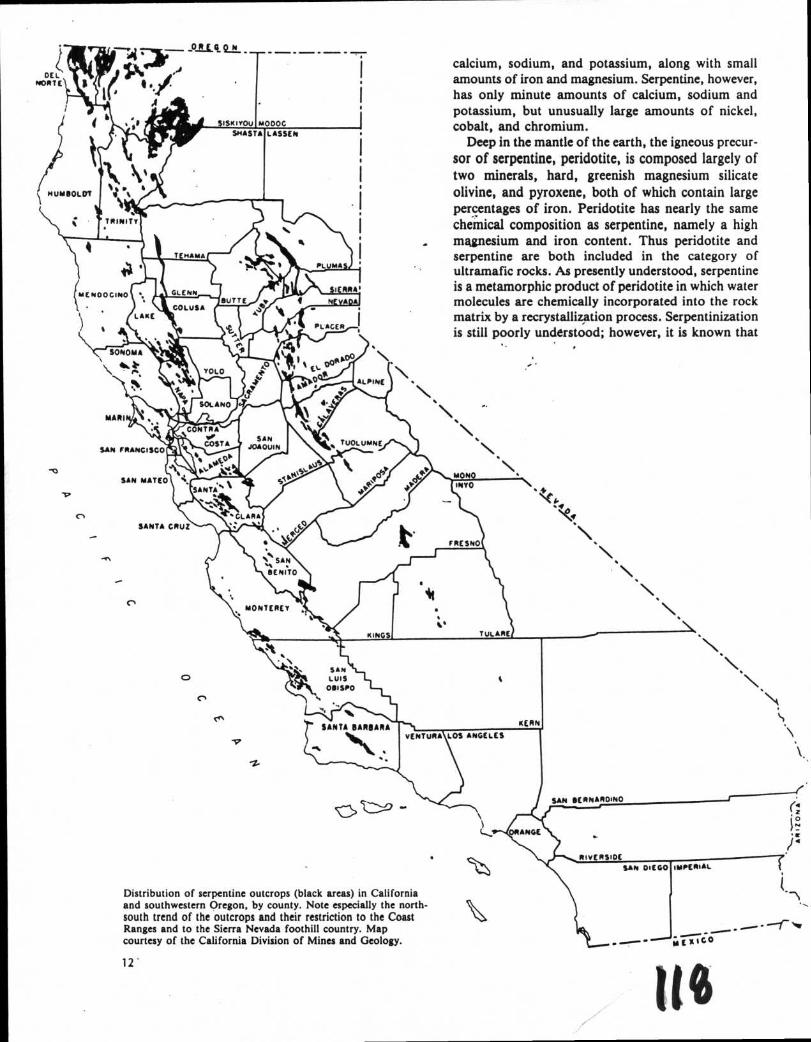
Distribution of serpentine outcrops (black areas) in California and southwestern Oregon, by county. Note especially the north-south trend of the outcrops and their restriction to the Coast Ranges and to the Sierra Nevada foothill country. Map courtesy of the California Division of Mines and Geology.

12

LOS ANGELES

SAN SERNARDINO

RIVERSIDE

T MAMA

PLACE

_o Jug_Q"- - -- -- -- _

SAN DIEGO IMPERIAL

,

- •-•"'"jxtC O

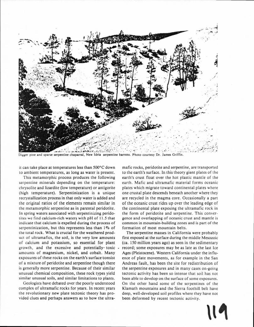
Digger pine and sparse serpentine chaparral, New Idria serpentine barrens. Photo courtesy Dr. James Griffin.

it can take place at temperatures less than 500°C down to ambient temperatures, as long as water is present.

This metamorphic process produces the following serpentine minerals depending on the temperature: chrysolite and lizardite (low temperature) or antigorite (high temperature). Serpentinization is a unique recrystallization process in that only water is added and the original ratios of the elements remain similar in the metamorphic serpentine as in parental peridotite. In spring waters associated with serpentinizing perido-tites we find calcium-rich waters with pH of 11.5 that indicate that calcium is expelled during the process of serpentinization, but this represents less than 1% of the total rock. What is crucial for the weathered prod-uct of ultramafics, the soil, is the very low amounts of calcium and potassium, so essential for plant growth, and the excessive and potentially- toxic amounts of magnesium, nickel, and cobalt. Many exposures of these rocks on the earth's surfaccconsist of a mixture of peridotite and serpentine though there is generally more serpentine. Because of their similar unusual chemical composition, these rock types yield similar unusual soils, and similar limitations to plants.

Geologists have debated over the poorly understood complex of ultramafic rocks for years. In recent years the revolutionary new plate tectonic theory has pro-vided clues and perhaps answers as to how the ultra-

mafic rocks, peridotite and serpentine, are transported to the earth's surface. In this theory giant plates of the earth's crust float over the hot plastic mantle of the earth. Mafic and ultramafic material forms oceanic plates which migrate toward continental plates where one crustal plate descends beneath another where they are recycled in the magma core. Occasionally a part of the oceanic crust rides up over the leading edge of the continental plate exposing the ultramafic rock in the form of peridotite and serpentine. This conver-gence and overlapping of oceanic crust and mantle is common in mountain-building zones and is part of the formation of most mountain belts.

The serpentine masses in California were probably first exposed at the surface during the middle Mesozoic (ca. 150 million years ago) as seen in the sedimentary record; some exposures may be as late as the last Ice Ages (Pleistocene). Western California under the influ-ence of plate movements, as for example in the San Andreas fault, has been the site for redistribution of the serpentine exposures and in many cases on-going tectonic activity has been so intense that soil has not been able to develop on the surface of some exposures. On the other hand some of the serpentines of the Klamath mountains and the Sierra foothill belt have deep, well-developed soil profiles where they have not been deformed by recent tectonic activity.

14

Distribution of Serpentine

From Oregon south to Santa Barbara and Tulare counties, eleven hundred square miles of serpentine and related rocks are distributed in numerous masses with discontinuous and northwest-trending orienta-tion. There are gaps in its distribution with essentially no outcrops in southern California (a tiny outcrop in the Santa Ana Mountains), none in the high Sierra or their eastern flanks, and none in the Great Valley or desert areas. Serpentine is a familiar sight in the South and North Coast ranges, the Klamath-Siskiyou coun-try and the lower western slopes of the Sierra.

A quick tour of California from north to south highlights the most important areas of serpentine or ultramafic rock occurrence. The Weed sheet of the state geologic maps covering the Klamath-Siskiyou area in northern California shows the most massive and extensive outcrops in the state. There is nearly

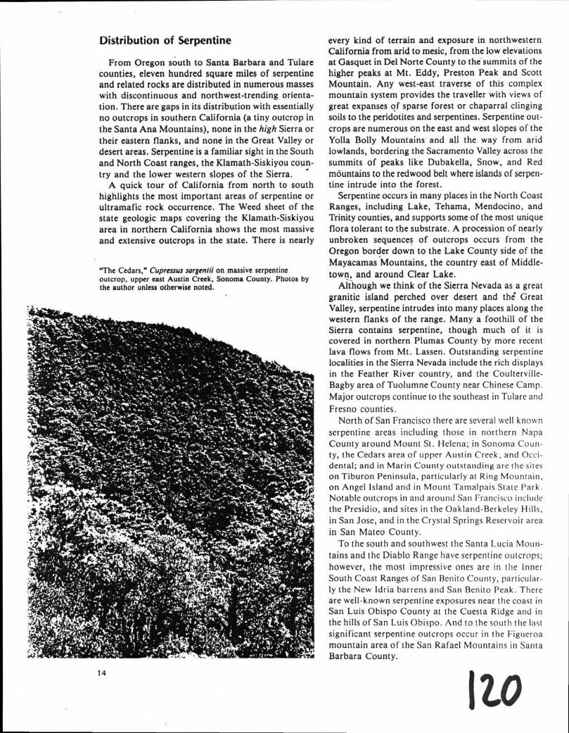
"The Cedars," Cupressus sargentii on massive serpentine outcrop, upper east Austin Creek, Sonoma County. Photos by the author unless otherwise noted.

every kind of terrain and exposure in northwestern California from arid to mesic, from the low elevations at Gasquet in Del Norte County to the summits of the higher peaks at Mt. Eddy, Preston Peak and Scott Mountain. Any west-east traverse of this complex mountain system provides the traveller with views of great expanses of sparse forest or chaparral clinging soils to the peridotites and serpentines. Serpentine out-crops are numerous on the east and west slopes of the Yolla Bolly Mountains and all the way from arid lowlands, bordering the Sacramento Valley across the summits of peaks like Dubakella, Snow, and Red mountains to the redwood belt where islands of serpen-tine intrude into the forest.

Serpentine occurs in many places in the North Coast Ranges, including Lake, Tehama, Mendocino, and Trinity counties, and supports some of the most unique flora tolerant to the substrate. A procession of nearly unbroken sequences of outcrops occurs from the Oregon border down to the Lake County side of the Mayacamas Mountains, the country east of Middle-town, and around Clear Lake.

Although we think of the Sierra Nevada as a great granitic island perched over desert and the Great Valley, serpentine intrudes into many places along the western flanks of the range. Many a foothill of the Sierra contains serpentine, though much of it is covered in northern Plumas County by more recent lava flows from Mt. Lassen. Outstanding serpentine localities in the Sierra Nevada include the rich displays in the Feather River country, and the Coulterville-Bagby area of Tuolumne County near Chinese Camp. Major outcrops continue to the southeast in Tulare and Fresno counties.

North of San Francisco there are several well known serpentine areas including those in northern Napa County around Mount St. Helena; in Sonoma Coun-ty, the Cedars area of upper Austin Creek, and Occi-dental; and in Marin County outstanding are the sites on Tiburon Peninsula, particularly at Ring Mountain, on Angel Island and in Mount Tamalpais State Park. Notable outcrops in and around San Francisco include the Presidio, and sites in the Oakland-Berkeley Hills, in San Jose, and in the Crystal Springs Reservoir area in San Mateo County.

To the south and southwest the Santa Lucia Moun-tains and the Diablo Range have serpentine outcrops; however, the most impressive ones are in the Inner South Coast Ranges of San Benito County, particular-ly the New Idria barrens and San Benito Peak. There are well-known serpentine exposures near the coast in San Luis Obispo County at the Cuesta Ridge and in the hills of San Luis Obispo. And to the south the last significant serpentine outcrops occur in the Figueroa mountain area of the San Rafael Mountains in Santa Barbara County.

1 20

react to weathering primarily by going into solution. Deeper serpentine soils are punky, pigmented residuals of iron oxides released during intense weathering of serpentine rock. Often soils derived from other rock types will wash down and cover serpentine rock, pro-viding a mistaken impression of a thick serpentine soil or of vegetative growth on serpentine soil and rock.

Considerable research has been done on the inability of serpentine soils to supply adequate nutrients for normal plant growth. Several University of Califor-nia scientists, Hans Jenny, James Vlamis, Perry Stout, C.M. Johnson and Richard B. Walker, all attributed the infertility of serpentine soil for plants to an im-balance between calcium and magnesium. Levels of nitrogen, phosphate and potassium (NPK), and the essential micronutrient molybdenum are low in most serpentine soils, while some can contain toxic amounts of nickel. When grown on serpentine soils, cultivated plants are depressed in growth and exhibit other defi-ciency symptoms corrected only with massive, repeated additions of gypsum (CaSO 4) and NPK.

So inhospitable a medium for plant growth has not stopped colonization of serpentine by some of the California flora. Species from many different plant families are able to tolerate the unusual chemical and physical qualities of these soils. Explanations for the mechanisms that provide this inherited tolerance of serpentine plants are only partially satisfactory. We now know that serpentine tolerant species are able to extract calcium and other essential elements in low supply in the soil better than plants not found on serpentines. Hans Jenny reminds us that the complex relationships between plants and soil involves the inter-play of many factors. For the network of factors that foster serpentine vegetation, Jenny has coined the term "serpentine syndrome," reminding us of the many linked strands of plant-soil interactions. In this con-cept the exceptional chemical composition of serpen-tine soil (low calcium, high magnesium, heavy metals, etc.) sets in motion a biological response that results in a low turnover of nitrogen and phosphorus. The low nutrient status and the cation imbalances result in a sparse plant cover and in turn a high heat budget at ground level. High temperature effects and moisture stress further check plant growth and survival. Since serpentine soils are usually derived from rock outcrops on steep or irregular topography, the habitats are often of unstable talus, adding a further stressful challenge to plants.

Plant Responses to Serpentine

Plants have a characteristic growth form on serpen-tine soils. Woody plants are either stunted or compact, and herbaceous species are often dwarfed. Leaves are

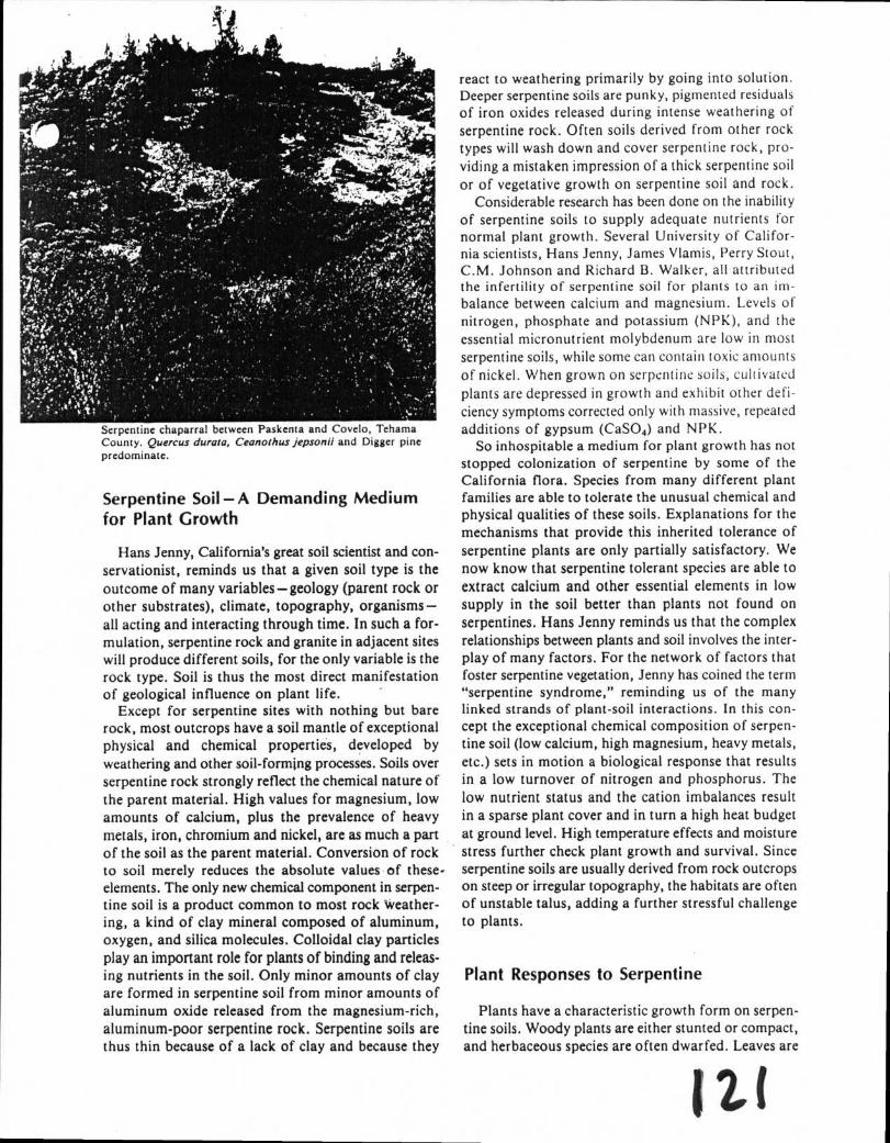
Serpentine chaparral between Paskenta and Covelo, Tehama County. Quercus durata, Ceanothus jepsonii and Digger pine

predominate.

Serpentine Soil—A Demanding Medium for Plant Growth

Hans Jenny, California's great soil scientist and con-servationist, reminds us that a given soil type is the outcome of many variables — geology (parent rock or other substrates), climate, topography, organisms—all acting and interacting through time. In such a for-mulation, serpentine rock and granite in adjacent sites will produce different soils, for the only variable is the rock type. Soil is thus the most direct manifestation of geological influence on plant life.

Except for serpentine sites with nothing but bare rock, most outcrops have a soil mantle of exceptional physical and chemical properties, developed by weathering and other soil-forming processes. Soils over serpentine rock strongly reflect the chemical nature of the parent material. High values for magnesium, low amounts of calcium, plus the prevalence of heavy metals, iron, chromium and nickel, are as much a part of the soil as the parent material. Conversion of rock to soil merely reduces the absolute values of these-elements. The only new chemical component in serpen-tine soil is a product common to most rock Weather-ing, a kind of clay mineral composed of aluminum, oxygen, and silica molecules. Colloidal clay particles play an important role for plants of binding and releas-ing nutrients in the soil. Only minor amounts of clay are formed in serpentine soil from minor amounts of aluminum oxide released from the magnesium-rich, aluminum-poor serpentine rock. Serpentine soils are thus thin because of a lack of clay and because they

• —"4111V•hs....•••■• ••••••■••-•-

.40

t:r. ••";,, s.%

T .4,

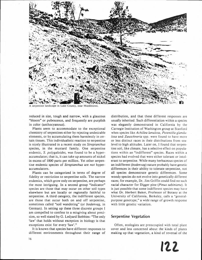
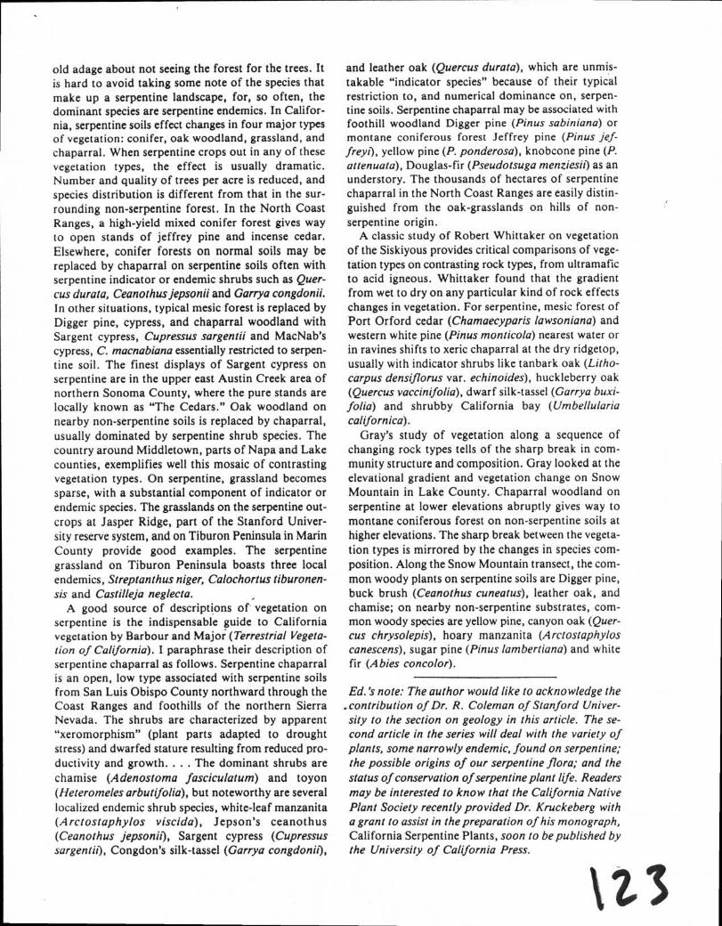
.7, A serpentine landscape in Lake County, near Middletown.

'

••••?•40611

,•• '

X'‘. •

k4 ;h

lak • • ■••,. •

Vii, t1 i• .

•

reduced in size, tough and narrow, with a glaucous

"bloom" or pubescence, and frequently are purplish

in color (anthocyanous). Plants seem to accommodate to the exceptional

chemistry of serpentines either by rejecting undesirable elements, or by accumulating them harmlessly in cer-tain tissues. This individualistic reaction to serpentine is nicely illustrated in a recent study on Streptanthus species, in the mustard family. One serpentine

endemic, S. polygaloides, was found to be a hyper-

accumulator; that is, it can take up amounts of nickel

in excess of 1000 parts per million. Yet other serpen-tine endemic species of Streptanthus are not hyper-

accumulators. Plants can be categorized in terms of degree of

fidelity or restriction to serpentine soils. The narrow endemics, which grow only on serpentine, are perhaps

the most intriguing. In a second group "indicator" species are those that may occur on other soil types elsewhere but are locally or regionally faithful to serpentine. A third category, the indifferent species, are those that occur both on and off serpentine, sometimes called "soil wandering" (or bodenvag, in

German). In setting up these three discrete groups I am compelled to confess to a misgiving about preci-

sion, so well stated by G. Ledyard Stebbins: "The only

'law' that holds without exception in biology is that

exceptions exist for every 'law'." It is known that species have different responses to

different environments throughout their range of

16

distribution, and that these different responses are

usually inherited. Such differentiation within a species

was elegantly demonstrated in California by the Carnegie Institution of Washington group at Stanford when species like Achillea lanulosa, Potentilla glandu-losa and Zauschneria spp. were found to have more

or less distinct races in their distributions from sea-level to high altitudes. Later on, I found that serpen-tine soil, like climate, has a selective effect on popula-

tions within an "indifferent" species. Races within a species had evolved that were either tolerant or intol-erant to serpentine. While many herbaceous species of an indifferent (bodenvag) nature probably have genetic differences in their ability to tolerate serpentine, not all species demonstrate genetic differences. Some woody species do not evolve into genetically different races; for example, Dr. Jim Griffin could find no such racial character for Digger pine (Pinus sabiniana). It is just possible that some indifferent species may have what Dr. Herbert Baker, Professor of Botany at the University of California, Berkeley, calls a "general-

purpose genotype," a wide range of growth response with little genetic variation.

Serpentine Vegetation

Often, ecologists are preoccupied with total plant cover and less concerned about the kinds of plants making up that vegetation, a kind of reversal of the

121

old adage about not seeing the forest for the trees. It is hard to avoid taking some note of the species that make up a serpentine landscape, for, so often, the dominant species are serpentine endemics. In Califor-nia, serpentine soils effect changes in four major types of vegetation: conifer, oak woodland, grassland, and chaparral. When serpentine crops out in any of these vegetation types, the effect is usually dramatic. Number and quality of trees per acre is reduced, and species distribution is different from that in the sur-rounding non-serpentine forest. In the North Coast Ranges, a high-yield mixed conifer forest gives way to open stands of jeffrey pine and incense cedar. Elsewhere, conifer forests on normal soils may be replaced by chaparral on serpentine soils often with serpentine indicator or endemic shrubs such as Quer-cus durata, Ceanothus jepsonii and Garrya congdonii. In other situations, typical mesic forest is replaced by Digger pine, cypress, and chaparral woodland with Sargent cypress, Cupressus sargentii and MacNab's cypress, C. macnabiana essentially restricted to serpen-tine soil. The finest displays of Sargent cypress on serpentine are in the upper east Austin Creek area of northern Sonoma County, where the pure stands are locally known as "The Cedars." Oak woodland on nearby non-serpentine soils is replaced by chaparral, usually dominated by serpentine shrub species. The country around Middletown, parts of Napa and Lake counties, exemplifies well this mosaic of contrasting vegetation types. On serpentine, grassland becomes sparse, with a substantial component of indicator or endemic species. The grasslands on the serpentine out-crops at Jasper Ridge, part of the Stanford Univer-sity reserve system, and on Tiburon Peninsula in Mahn County provide good examples. The serpentine grassland on Tiburon Peninsula boasts three local endemics, Streptanthus niger, Calochortus tiburonen-sis and Castilleja neglecta.

A good source of descriptions of vegetation on serpentine is the indispensable guide to California vegetation by Barbour and Major (Terrestrial Vegeta-tion of California). I paraphrase their description of serpentine chaparral as follows. Serpentine chaparral is an open, low type associated with serpentine soils from San Luis Obispo County northward through the Coast Ranges and foothills of the northern Sierra Nevada. The shrubs are characterized by apparent "xeromorphism" (plant parts adapted to drought stress) and dwarfed stature resulting from reduced pro-ductivity and growth. . . . The dominant shrubs are chamise (Adenostoma fasciculatum) and toyon (Heteromeles arbutifolia), but noteworthy are several localized endemic shrub species, white-leaf manzanita (Arctostaphylos viscida), Jepson's ceanothus (Ceanothus jepsonii), Sargent cypress (Cupressus sargentii), Congdon's silk-tassel (Garrya congdonii),

and leather oak (Quercus durata), which are unmis-takable "indicator species" because of their typical restriction to, and numerical dominance on, serpen-tine soils. Serpentine chaparral may be associated with foothill woodland Digger pine (Pinus sabiniana) or montane coniferous forest Jeffrey pine (Pinus jef-freyi), yellow pine (P. ponderosa), knobcone pine (P. attenuata), Douglas-fir (Pseudotsuga menziesii) as an understory. The thousands of hectares of serpentine chaparral in the North Coast Ranges are easily distin-guished from the oak-grasslands on hills of non-serpentine origin.

A classic study of Robert Whittaker on vegetation of the Siskiyous provides critical comparisons of vege-tation types on contrasting rock types, from ultramafic to acid igneous. Whittaker found that the gradient from wet to dry on any particular kind of rock effects changes in vegetation. For serpentine, mesic forest of Port Orford cedar (Chamaecyparis lawsoniana) and western white pine (Pinus monticola) nearest water or in ravines shifts to xeric chaparral at the dry ridgetop, usually with indicator shrubs like tanbark oak (Litho-carpus densiflorus var. echinoides), huckleberry oak (Quercus vaccinifolia), dwarf silk-tassel (Garrya buxi-folia) and shrubby California bay (Umbellularia californica).

Gray's study of vegetation along a sequence of changing rock types tells of the sharp break in com-munity structure and composition. Gray looked at the elevational gradient and vegetation change on Snow Mountain in Lake County. Chaparral woodland on serpentine at lower elevations abruptly gives way to montane coniferous forest on non-serpentine soils at higher elevations. The sharp break between the vegeta-tion types is mirrored by the changes in species com-position. Along the Snow Mountain transect, the com-mon woody plants on serpentine soils are Digger pine, buck brush (Ceanothus cuneatus), leather oak, and chamise; on nearby non-serpentine substrates, com-mon woody species are yellow pine, canyon oak (Quer-cus chrysolepis), hoary manzanita (A rctostaphylos canescens), sugar pine (Pinus lambertiana) and white fir (Abies concolor).

Ed.'s note: The author would like to acknowledge the .contribution of Dr. R. Coleman of Stanford Univer-sity to the section on geology in this article. The se-cond article in the series will deal with the variety of plants, some narrowly endemic, found on serpentine; the possible origins of our serpentine flora; and the status of conservation of serpentine plant life. Readers may be interested to know that the California Native Plant Society recently provided Dr. Kruckeberg with a grant to assist in the preparation of his monograph, California Serpentine Plants, soon to be published by the University of California Press.

123

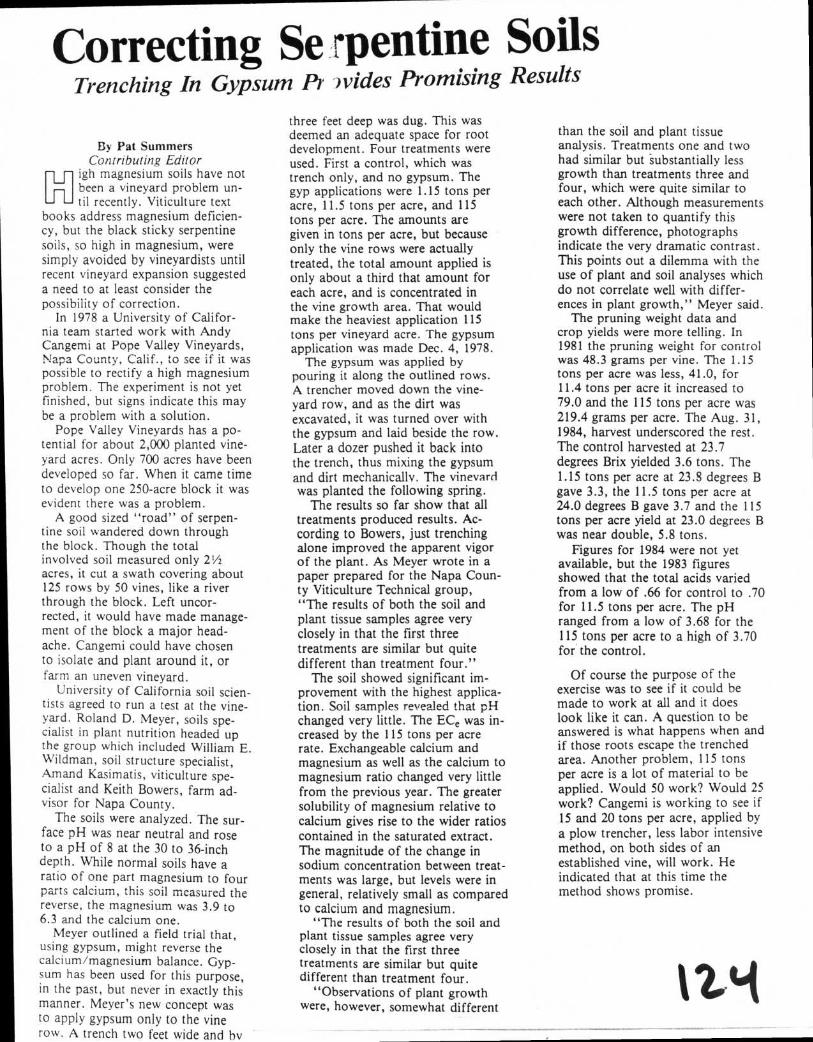
Correcting Serpentine Soils Trenching In Gypsum Pr )vides Promising Results

By Pat Summers Contributing Editor

igh magnesium soils have not been a vineyard problem un-

-F1- til recently. Viticulture text books address magnesium deficien-cy, but the black sticky serpentine soils, so high in magnesium, were simply avoided by vineyardists until recent vineyard expansion suggested a need to at least consider the possibility of correction.

In 1978 a University of Califor-nia team started work with Andy Cangemi at Pope Valley Vineyards, Napa County, Calif., to see if it was possible to rectify a high magnesium problem. The experiment is not yet finished, but signs indicate this may be a problem with a solution.

Pope Valley Vineyards has a po-tential for about 2,000 planted vine-yard acres. Only 700 acres have been developed so far. When it came time to develop one 250-acre block it was evident there was a problem.

A good sized "road" of serpen-tine soil wandered down through the block. Though the total involved soil measured only 21/2 acres, it cut a swath covering about 125 rows by 50 vines, like a river through the block. Left uncor-rected, it would have made manage-ment of the block a major head-ache. Cangemi could have chosen to isolate and plant around it, or farm an uneven vineyard.

University of California soil scien-tists agreed to run a test at the vine-yard. Roland D. Meyer, soils spe-cialist in plant nutrition headed up the group which included William E. Wildman, soil structure specialist, Arnand Kasimatis, viticulture spe-cialist and Keith Bowers, farm ad-visor for Napa County.

The soils were analyzed. The sur-face pH was near neutral and rose to a pH of 8 at the 30 to 36-inch depth. While normal soils have a ratio of one part magnesium to four parts calcium, this soil measured the reverse, the magnesium was 3.9 to 6.3 and the calcium one.

Meyer outlined a field trial that, using gypsum, might reverse the calcium/magnesium balance. Gyp-sum has been used for this purpose, in the past, but never in exactly this manner. Meyer's new concept was to apply gypsum only to the vine row. A trench two feet wide and by

three feet deep was dug. This was deemed an adequate space for root development. Four treatments were used. First a control, which was trench only, and no gypsum. The gyp applications were 1.15 tons per acre, 11.5 tons per acre, and 115 tons per acre. The amounts are given in tons per acre, but because only the vine rows were actually treated, the total amount applied is only about a third that amount for each acre, and is concentrated in the vine growth area. That would make the heaviest application 115 tons per vineyard acre. The gypsum application was made Dec. 4, 1978.

The gypsum was applied by pouring it along the outlined rows. A trencher moved down the vine-yard row, and as the dirt was excavated, it was turned over with the gypsum and laid beside the row. Later a dozer pushed it back into the trench, thus mixing the gypsum and dirt mechanically. The vineyard was planted the following spring.

The results so far show that all treatments produced results. Ac-cording to Bowers, just trenching alone improved the apparent vigor of the plant. As Meyer wrote in a paper prepared for the Napa Coun-ty Viticulture Technical group, "The results of both the soil and plant tissue samples agree very closely in that the first three treatments are similar but quite different than treatment four."

The soil showed significant im-provement with the highest applica-tion. Soil samples revealed that pH changed very little. The ECe was in-creased by the 115 tons per acre rate. Exchangeable calcium and magnesium as well as the calcium to magnesium ratio changed very little from the previous year. The greater solubility of magnesium relative to calcium gives rise to the wider ratios contained in the saturated extract. The magnitude of the change in sodium concentration between treat-ments was large, but levels were in general, relatively small as compared to calcium and magnesium.

"The results of both the soil and plant tissue samples agree very closely in that the first three treatments are similar but quite different than treatment four.

"Observations of plant growth were, however, somewhat different

than the soil and plant tissue analysis. Treatments one and two had similar but substantially less growth than treatments three and four, which were quite similar to each other. Although measurements were not taken to quantify this growth difference, photographs indicate the very dramatic contrast. This points out a dilemma with the use of plant and soil analyses which do not correlate well with differ-ences in plant growth," Meyer said.

The pruning weight data and crop yields were more telling. In 1981 the pruning weight for control was 48.3 grams per vine. The 1.15 tons per acre was less, 41.0, for 11.4 tons per acre it increased to 79.0 and the 115 tons per acre was 219.4 grams per acre. The Aug. 31, 1984, harvest underscored the rest. The control harvested at 23.7 degrees Brix yielded 3.6 tons. The 1.15 tons per acre at 23.8 degrees B gave 3.3, the 11.5 tons per acre at 24.0 degrees B gave 3.7 and the 115 tons per acre yield at 23.0 degrees B was near double, 5.8 tons.

Figures for 1984 were not yet available, but the 1983 figures showed that the total acids varied from a low of .66 for control to .70 for 11.5 tons per acre. The pH ranged from a low of 3.68 for the 115 tons per acre to a high of 3.70 for the control.

Of course the purpose of the exercise was to see if it could be made to work at all and it does look like it can. A question to be answered is what happens when and if those roots escape the trenched area. Another problem, 115 tons per acre is a lot of material to be applied. Would 50 work? Would 25 work? Cangemi is working to see if 15 and 20 tons per acre, applied by a plow trencher, less labor intensive method, on both sides of an established vine, will work. He indicated that at this time the method shows promise.

I/4

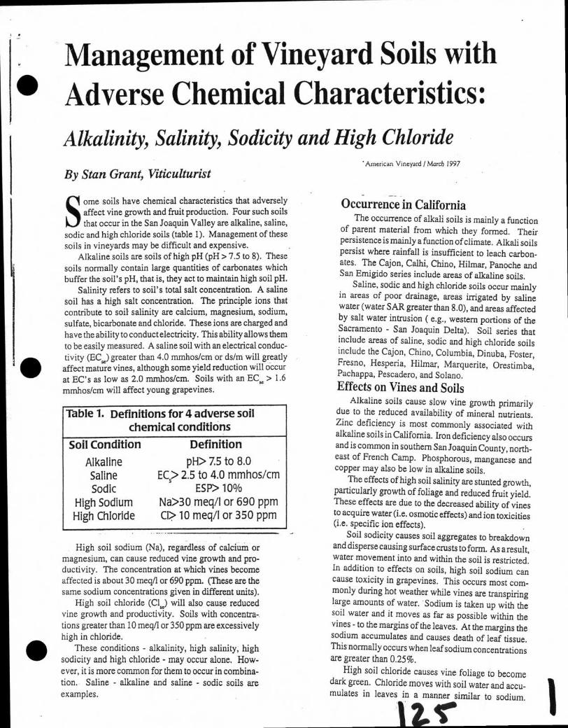
Table 1. Definitions for 4 adverse soil chemical conditions

Soil Condition Definition Alkaline Saline Sodic

High Sodium High Chloride

pH> 7.5 to 8.0 Ec> 2.5 to 4.0 mmhos/cm

ESP> 10% Na>30 meq/1 or 690 ppm Cl> 10 meq/I or 350 ppm

Management of Vineyard Soils with Adverse Chemical Characteristics: Alkalinity, Salinity, Sodicity and High Chloride

'American Vineyard / March 1997

•

By Stan Grant, Viticulturist

S ome soils have chemical characteristics that adversely affect vine growth and fruit production. Four such soils that occur in the San Joaquin Valley are alkaline, saline,

sodic and high chloride soils (table 1). Management of these soils in vineyards may be difficult and expensive. .

Alkaline soils are soils of high pH (pH > 7.5 to 8). These soils normally contain large quantities of carbonates which buffer the soil's pH, that is, they act to maintain high soil pH.

Salinity refers to soil's total salt concentration. A saline soil has a high salt concentration. The principle ions that contribute to soil salinity are calcium, magnesium, sodium, sulfate, bicarbonate and chloride. These ions are charged and have the ability to conduct electricity. This ability allows them to be easily measured. A saline soil with an electrical conduc-tivity (EC.) greater than 4.0 mmhos/cm or ds/m will greatly

affect mature vines, although some yield reduction will occur at EC's as low as 2.0 mmhos/cm. Soils with an EC. > 1.6 mmhos/cm will affect young grapevines.

High soil sodium (Na), regardless of calcium or magnesium, can cause reduced vine growth and pro-ductivity. The concentration at which vines become affected is about 30 meq/1 or 690 ppm. (These are the same sodium concentrations given in different units).

High soil chloride (Cl). will also cause reduced vine growth and productivity. Soils with concentra- . tions greater than 10 meq/1 or 350 ppm are excessively high in chloride.

These conditions - alkalinity, high salinity, high sodicity and high chloride - may occur alone. How-ever, it is more common for them to occur in combina-tion. Saline - alkaline and saline - sodic soils are examples.

Occurrence in California The occurrence of alkali soils is mainly a function

of parent material from which they formed. Their persistence is mainly a function of climate. Alkali soils persist where rainfall is insufficient to leach carbon-ates. The Cajon, Calhi, Chino, Hilmar, Panoche and San Emigido series include areas of alkaline soils.

Saline, sodic and high chloride soils occur mainly in areas of poor drainage, areas irrigated by saline water (water SAR greater than 8.0), and areas affected by salt water intrusion ( e.g., western portions of the Sacramento - San Joaquin Delta). Soil series that include areas of saline, sodic and high chloride soils include the Cajon, Chino, Columbia, Dinuba, Foster, Fresno, Hesperia, Hilmar, Marguerite, Orestimba, Pachappa, Pescadero, and Solano. Effects on Vines and Soils

Alkaline soils cause slow vine growth primarily due to the reduced availability of mineral nutrients. Zinc deficiency is most commonly associated with alkaline soils in California. Iron deficiency also occurs and is common in southern San Joaquin County, north-east of French Camp. Phosphorous, manganese and copper may also be low in alkaline soils.

The effects of high soil salinity are stunted growth, particularly growth of foliage and reduced fruit yield. These effects are due to the decreased ability of vines to acquire water (i.e. osmotic effects) and ion toxicities (i.e. specific ion effects).

Soil sodicity causes soil aggregates to breakdown and disperse causing surface crusts to form. As a result, water movement into and within the soil is restricted. In addition to effects on soils, high soil sodium can cause toxicity in grapevines. This occurs most com-monly during hot weather while vines are transpiring large amounts of water. Sodium is taken up with the soil water and it moves as far as possible within the vines - to the margins of the leaves. At the margins the sodium accumulates and causes death of leaf tissue. This normally occurs when leaf sodium concentrations are greater than 0.25%.

High soil chloride causes vine foliage to become dark green. Chloride moves with soil water and accu-mulates in leaves in a manner similar to sodium.

•

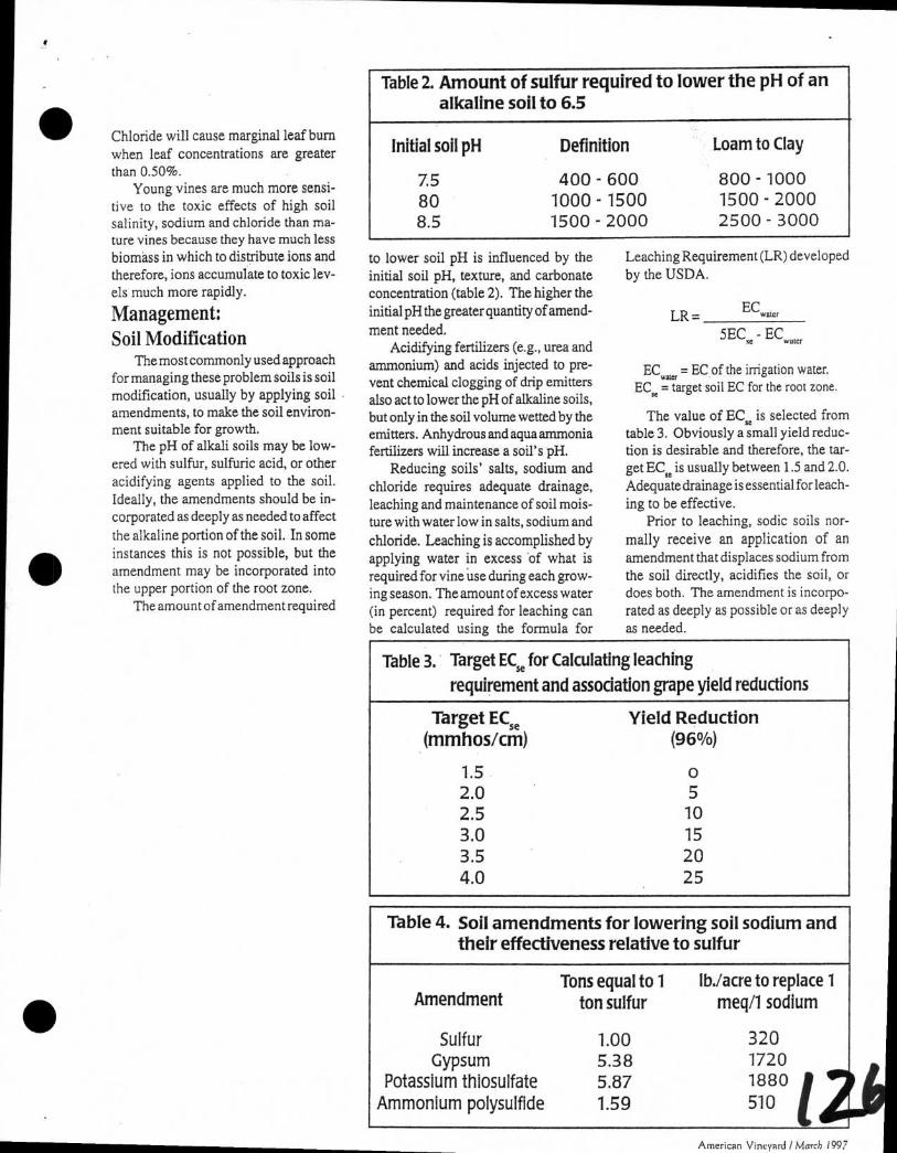
Table 2. Amount of sulfur required to lower the pH of an alkaline soil to 6.5

Initial soil pH Definition Loam to Clay

7.5 400 - 600 800 - 1000 80 1000 - 1500 1500 - 2000 8.5 1500 - 2000 2500 - 3000

Table 3. Target ECse for Calculating leaching requirement and association grape yield reductions

Target ECse (mmhos/cm)

Yield Reduction (96%)

1.5 0

2.0 5 2.5 10 3.0 15 3.5 20 4.0 25

Table 4. Soil amendments for lowering soil sodium and their effectiveness relative to sulfur

Amendment Tons equal to 1 Iblacre to replace 1

ton sulfur meq/1 sodium

Sulfur 1.00 Gypsum 5.38

Potassium thiosulfate 5.87 Ammonium polysulfide 1.59

320 1720 1880 510

American Vineyard / March 1997

• Chloride will cause marginal leaf bum when leaf concentrations are greater than 0.50%.

Young vines are much more sensi-tive to the toxic effects of high soil salinity, sodium and chloride than ma-ture vines because they have much less biomass in which to distribute ions and therefore, ions accumulate to toxic lev-els much more rapidly.

Management: Soil Modification

The most commonly used approach for managing these problem soils is soil modification, usually by applying soil amendments, to make the soil environ-ment suitable for growth.

The pH of alkali soils may be low-ered with sulfur, sulfuric acid, or other acidifying agents applied to the soil. Ideally, the amendments should be in-corporated as deeply as needed to affect the alkaline portion of the soil. In some instances this is not possible, but the amendment may be incorporated into the upper portion of the root zone.

The amount of amendment required

to lower soil pH is influenced by the initial soil pH, texture, and carbonate concentration (table 2). The higher the initial pH the greater quantity of amend-ment needed.

Acidifying fertilizers (e.g., urea and ammonium) and acids injected to pre-vent chemical clogging of drip emitters also act to lower the pH of alkaline soils, but only in the soil volume wetted by the emitters. Anhydrous and aqua ammonia fertilizers will increase a soil's pH.

Reducing soils' salts, sodium and chloride requires adequate drainage, leaching and maintenance of soil mois-ture with water low in salts, sodium and chloride. Leaching is accomplished by applying water in excess of what is required for vine use during each grow-ing season. The amount of excess water (in percent) required for leaching can be calculated using the formula for

Leaching Requirement (LR) developed by the USDA.

, LR =

Ecatc

5EC-EC

ECW = EC of the irrigation water. EC. = target soil EC for the root zone.

The value of EC. is selected from table 3. Obviously a small yield reduc-tion is desirable and therefore, the tar-get EC, is usually between 1.5 and 2.0. Adequate drainage is essential for leach-ing to be effective.

Prior to leaching, sodic soils nor-mally receive an application of an amendment that displaces sodium from the soil directly, acidifies the soil, or does both. The amendment is incorpo-rated as deeply as possible or as deeply as needed.

Table 5. Rootstock adaptation for 4 adverse soil chemical conditions

Soil Condition Well Adapted

Poorly Adapted

Alkaline

5BB, 420A, 140Ru

3309- 44-53, 101-14

Saline

Salt Creek, Dogridge

Own roots, Freedom, 101-14, 140Ru, 1616

420A, SO4

Sodic Salt Creek, Schwarzmann Own roots, Freedom

High Chloride Salt Creek, Schwarzmann, Own roots SO4, 5BB, 99R,

St. George, 101-14

Gypsum is frequently used to amend sodic soils. It serves as a source of calcium. Soils retain calcium more readily than they do sodium. This char-acteristic of calcium allows it to displace sodium from the soil. Application rates of gypsum are usually between 1 and 4 tons/acre and are rarely greater than 10 tons/acre. The amount of gypsum re-quired to replace soil sodium can be estimated with a laboratory test called the Gypsum Requirement. Gypsum may be either applied directly to the soil or with irrigation water.

If sodic soil contains high levels of carbonates, calcium is already present in the soil and may be released from the carbonates with the addition of sulfur or other acidifying amendments. Sulfur is more effective than gypsum in reduc-ing soil sodium (table 4). An agricul-tural laboratory can determine if car-bonates are present in the soil.

Amendments that both displace so-dium directly and acidify the soil in-clude potassium thiosulfate and ammo-nium polysulfide.

Management: Tolerant Rootstocks

Tolerant rootstocks are another im-portant component of managing alka-line, saline, sodic, and high chloride soils. Tolerant rootstocks will rarely substitute for modification of these prob-lem soils, but they lower the amount of amendments required.

To my knowledge, no studies on rootstock tolerance to soil alkalinity have been reported in the United States. However, in France many soils contain high levels of lime and vines grown in these soils frequently suffer from iron deficiency. Given that lime is another name for calcium carbonate, it seems highly probable that these soils are al-kaline. Rootstocks that have been shown to tolerate high lime soils in France include 5BB, 420A, and 140Ru. Roostocks that do poorly in these soils include 3309, 44-53 and 101-14.

Salt Creek, Dodgeridge, 101-14 and 140Ru are tolerant of saline soils. In southern France, 1616 is used success-fully on saline soils. Own rooted vines and vines on Freedom, 420, and SO4 poorly adapt to saline soils.

Rootstocks are practically the same. Salt Creek, Schwarzmann, SO4, 5BB, 99R, St. George and 101-14 are well

adapted to high chloride soils. Own rooted vines are poorly adapted to high chloride soils.

Rootstock Summary: 1. 140Ru is well adapted to alkaline

and saline soils. 2. 101-14 is well adapted to saline

and high chloride soils, but poorly adapted to alkaline soils.

3. 420 is well adapted to alkaline soils, but poorly adapted to saline soils. 420A is a low vigor rootstock and may not be appropriate for production-ori-ented vineyards in the San Joaquin Valley.

4. Salt Creek and Schwarzmann (and probably 99R) are well adapted to saline, high sodium and high chloride soils.

5. Avoid own rooted vines and Freedom for use in saline, high sodium and high chloride soils.

Summary Management of alkaline, saline, sodic

and high chloride vineyard soils nor-mally involves multiple viticulture prac-

tices including the use of tolerant rootstocks, soil amendments and thoughtfully applied irrigations. The combination of tolerant rootstocks and careful irrigation management may be sufficient when these adverse chemical conditions are very mild. Both practices are a part of normal vineyard operations, and, therefore, require little additional expense. Drainage improvement prior to planting may be needed, which adds greatly to development costs.

More severe soil chemical condi-tions require soil amendments. Soil amendments have to be reapplied when their effects diminish and chemical con-ditions worsen. Soil testing at regular intervals will reveal if and when reap-plication is necessary. Management of extreme conditions may not be practi-cal or economically feasible.

Vines growing in soil with adverse chemical characteristics are frequently smaller than normal. Spacing vines closer in the row will compensate for smaller vine size and maximize fruit production. cD)

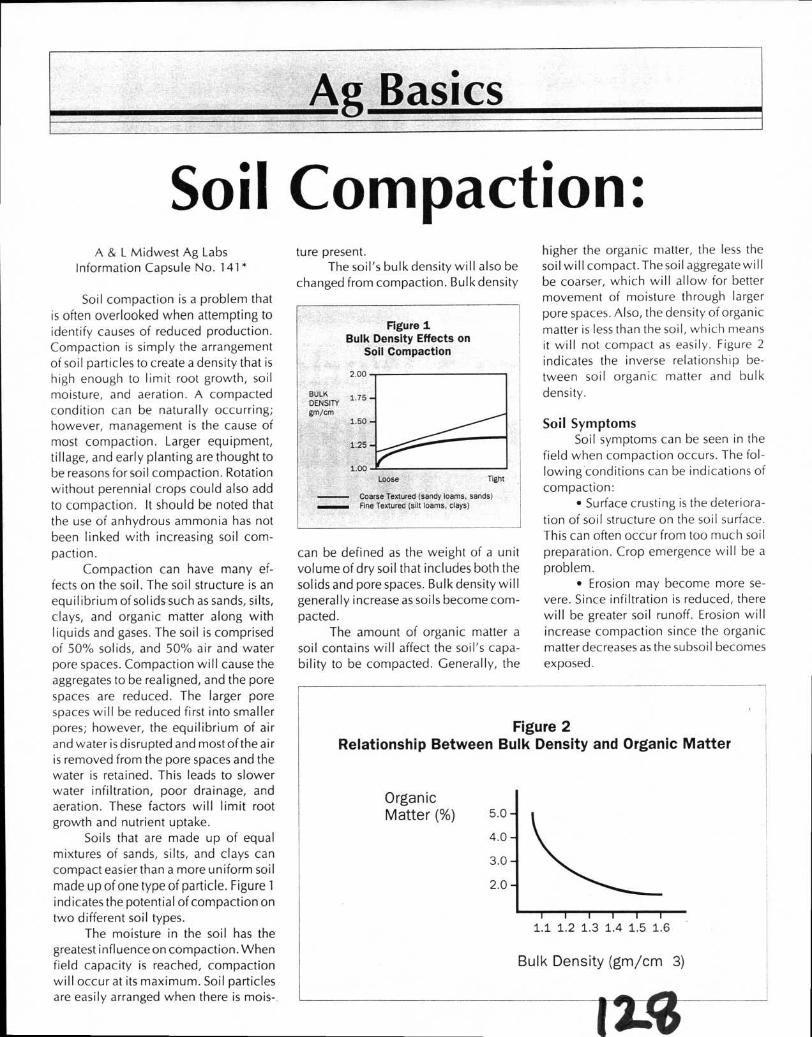
Figure 1 Bulk Density Effects on

Soil Compaction

2.00

BULK 1.75 DENSITY gm/cm

1.50

1.25

1.00

Loose Tight

Coarse Textured (sandy loams, sands) Fine Textured (silt !owns, clays)

j

Figure 2 Relationship Between Bulk Density and Organic Matter

Organic Matter (%)

1.1 1.2 1.3 1.4 1.5 1.6

Bulk Density (gm/cm 3)

1w3

Ag Basics

Soil Compaction: A & L Midwest Ag Labs

Information Capsule No. 141*

Soil compaction is a problem that

is often overlooked when attempting to

identify causes of reduced production. Compaction is simply the arrangement

of soil particles to create a density that is high enough to limit root growth, soil

moisture, and aeration. A compacted condition can be naturally occurring; however, management is the cause of

most compaction. Larger equipment, tillage, and early planting are thought to

be reasons for soil compaction. Rotation

without perennial crops could also add

to compaction. It should be noted that the use of anhydrous ammonia has not

been linked with increasing soil com-

paction. Compaction can have many ef-

fects on the soil. The soil structure is an equilibrium of solids such as sands, silts, clays, and organic matter along with

liquids and gases. The soil is comprised of 50% solids, and 50% air and water

pore spaces. Compaction will cause the aggregates to be realigned, and the pore

spaces are reduced. The larger pore spaces will be reduced first into smaller

pores; however, the equilibrium of air

and water is disrupted and most of the air

is removed from the pore spaces and the water is retained. This leads to slower water infiltration, poor drainage, and aeration. These factors will limit root growth and nutrient uptake.

Soils that are made up of equal mixtures of sands, silts, and clays can

compact easier than a more uniform soil

made up of one type of particle. Figure 1 indicates the potential of compaction on two different soil types.

The moisture in the soil has the greatest influence on compaction. When

field capacity is reached, compaction

will occur at its maximum. Soil particles are easily arranged when there is mois- .

ture present. The soil's bulk density will also be

changed from compaction. Bulk density

can be defined as the weight of a unit

volume of dry soil that includes both the

solids and pore spaces. Bulk density will generally increase as soils become com-

pacted. The amount of organic matter a

soil contains will affect the soil's capa-bility to be compacted. Generally, the

higher the organic matter, the less the soil will compact. The soil aggregate will be coarser, which will allow for better movement of moisture through larger

pore spaces. Also, the density of organic

matter is less than the soil, which means it will not compact as easily. Figure 2

indicates the inverse relationship be-tween soil organic matter and bulk

density.

Soil Symptoms Soil symptoms can be seen in the

field when compaction occurs. The fol-

lowing conditions can be indications of

compaction: • Surface crusting is the deteriora-

tion of soil structure on the soil surface.

This can often occur from too much soil

preparation. Crop emergence will be a

problem. • Erosion may become more se-

vere. Since infiltration is reduced, there

will be greater soil runoff. Erosion will

increase compaction since the organic

matter decreases as the subsoil becomes exposed.

High Low

Figure 4 Effects of Moisture and Bulk

Density on Compaction

Pressure

Low

Low

Bulk Density

High

High

Figure 3 Plant Height of Corn Reduced from Compaction

Average Plant Height (in.)

Compacted Moderately Not Compacted Compacted

128 —121-114 — 107 —100 —

Ag Basics

A Review • Standing water is also a symptom

of compaction. The porosity is decreased from compaction, which reduces infil-tration. Infiltration can be reduced by up to 16 times when these pore spaces are compacted.

• Herbicide problems can also

occur when a soil is compacted. The movement of the herbicide into the soil can be slowed since porosity is reduced. There can also be higher rates of carry-over with herbicides that rely on micro-bial activity for breakdown. The effi-ciency of the microbes under compacted conditions is reduced considerably.

Plant Symptoms The condition of the plants will

show the effects of compaction and soil symptoms described earlier. There are many plant symptoms of compaction. These can be seen in both the above-ground portion and root system.

Slow emergence will often occur when soils are compacted. The surface crust will stress the young seedlings and delay emergence. The soils may also be wet and cool due to poor internal drain-age from compaction. This will lead to disease associated with the seed.

Uneven growth early in the season

will also be a symptom of compaction. This also is due to poor aeration and reduced nutrient uptake when soils are wet and cool. This uneven growth will often continue through the season. Fig-ure 3 indicates the difference in plant height at various rates of compaction.

Purple color in corn plants is also a symptom of compaction. Poor internal drainage will reduce production of sug-ars in the plant. When this occurs, the plant will begin to produce a more promi-nent red pigment. Certain hybrids may tend to show this symptom more often.

Rooting patterns are also affected

by compaction. Often, a fibrous root system will grow horizontally along a compacted layer. This root system will generally be shallower, and moisture stress can be a problem under dry condi-tions. Lodging can also be a symptom when compaction is present. The uptake of the potassium will often be reduced in compacted soils. Research has shown an increased rate of lodging as the potas-sium decreases in relationship to the nitrogen level.

Measuring soil compaction can be very difficult since there are many para-meters that will affect the compaction. A soil penetrometer can be used to meas-

ure compaction in the field. This is the measurement of pressure required to move the tip of a shaft through the soil at a constant rate. The moisture content of the soil will have an effect on compac-tion readings. As the soil moisture in-creases, the amount of pressure required to move through the soil will be re-duced. Figure 4 indicates the lower amount of pressure required as the soil moisture increases at various bulk densi-ties.

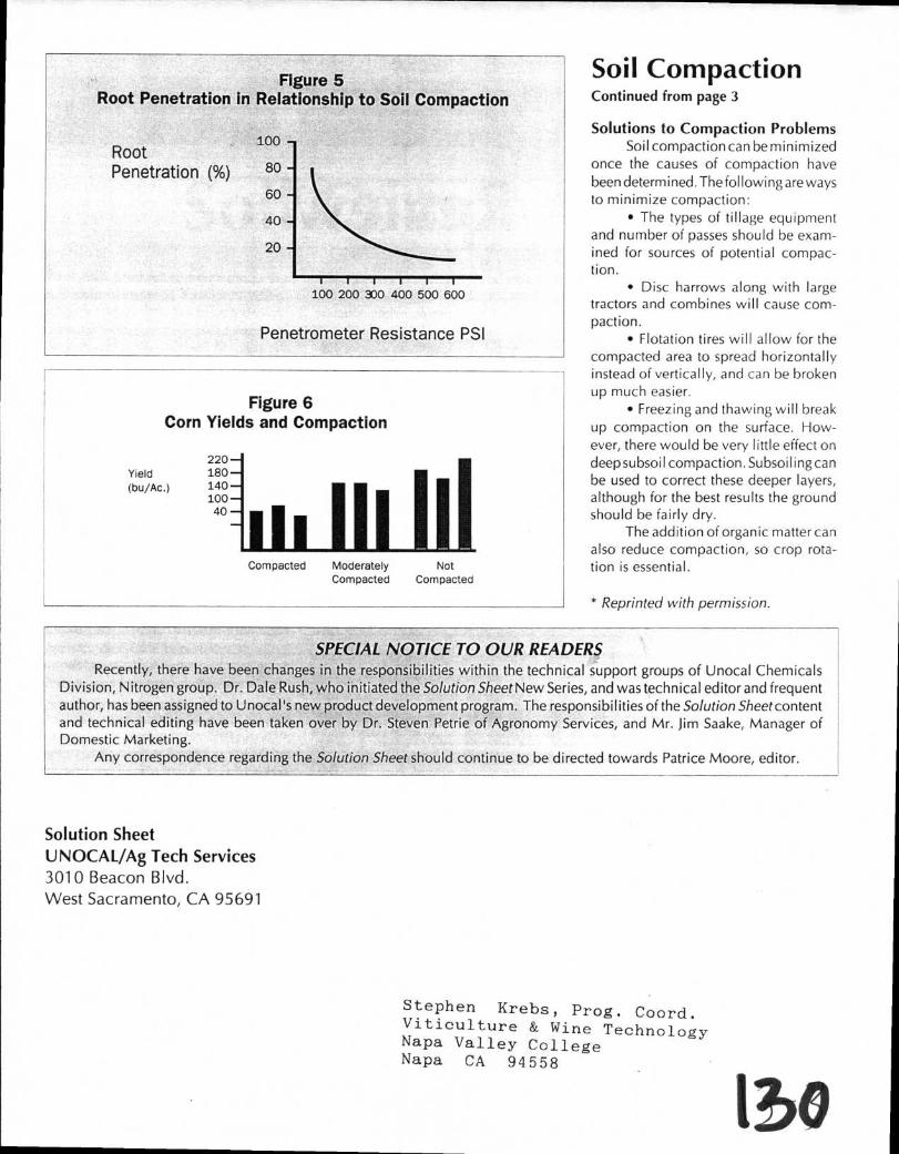
To determine the actual amount of compaction with a penetrometer, addi-tional analyses such as soil moisture and bulk density must be performed. How-ever, a penetrometer can be used to compare areas in a field that would be similar in soil moisture and bulk density for compaction. Crops may be affected differently in terms of root restriction and crop yield. Figure 5 shows an approxi-mate reduction curve for most fibrous root crops such as corn and small grains. However, this will shift, depending on the rooting nature of various crops.

Compaction can reduce crop yields as shown in Figure 6. Corn yields were reduced significantly in compacted ar-eas in comparison with noncompactgd fields.

Continued on page 4

100 -

80 -

60 -

40 -

20 -

Root Penetration (%)

I 100 200 300 400 500 600

Penetrometer Resistance PSI

220-180-140-100-40—

Yield (bu/Ac.)

II. III hi

Figure 5 Root Penetration in Relationship to Soil Compaction

Figure 6 Corn Yields and Compaction

Compacted Moderately Not Compacted Compacted

So il Compact i on Continued from page 3

Solutions to Compaction Problems Soil compaction can be minimized

once the causes of compaction have been determined. The following are ways to minimize compaction:

• The types of tillage equipment and number of passes should be exam-ined for sources of potential compac-tion.

• Disc harrows along with large tractors and combines will cause com-paction.

• Flotation tires will allow for the compacted area to spread horizontally instead of vertically, and can be broken up much easier.

• Freezing and thawing will break up compaction on the surface. How-ever, there would be very little effect on deep subsoil compaction. Subsoil ing can be used to correct these deeper layers, although for the best results the ground should be fairly dry.

The addition of organic matter can also reduce compaction, so crop rota-tion is essential.

* Reprinted with permission.

SPECIAL NOTICE TO OUR READERS Recently, there have been changes in the responsibilities within the technical support groups of Unocal Chemicals

Division, Nitrogen group. Dr. Dale Rush, who initiated the Solution Sheet New Series, and was technical editor and frequent author, has been assigned to Unocal's new product development program. The responsibilities of the Solution Sheet content and technical editing have been taken over by Dr. Steven Petrie of Agronomy Services, and Mr. Jim Saake, Manager of Domestic Marketing.

Any correspondence regarding the Solution Sheet should continue to be directed towards Patrice Moore, editor.

Solution Sheet UNOCAL/Ag Tech Services 3010 Beacon Blvd. West Sacramento, CA 95691

Stephen Krebs, Prog. Coord. Viticulture & Wine Technology Napa Valley College Napa CA 94558

150