California State Waters Map Series—Offshore of Ventura, California · Ventura” map area (figs....

California State Waters Map Series—Offshore of Ventura, California

By Samuel Y. Johnson, Peter Dartnell, Guy R. Cochrane, Nadine E. Golden, Eleyne L. Phillips, Andrew C. Ritchie, Rikk G. Kvitek, H. Gary Greene, Lisa M. Krigsman, Charles A. Endris, Gordon G. Seitz, Carlos I. Gutierrez, Ray W. Sliter, Mercedes D. Erdey, Florence L. Wong, Mary M. Yoklavich, Amy E. Draut, and Patrick E. Hart

(Samuel Y. Johnson and Susan A. Cochran, editors)

Pamphlet to accompany

Scientific Investigations Map 3254

2013

U.S. Department of the Interior U.S. Geological Survey

U.S. Department of the Interior KEN SALAZAR, Secretary

U.S. Geological Survey Suzette M. Kimball, Acting Director

U.S. Geological Survey, Reston, Virginia: 2013

For more information on the USGS—the Federal source for science about the Earth,

its natural and living resources, natural hazards, and the environment—visit

http://www.usgs.gov or call 1–888–ASK–USGS

For an overview of USGS information products, including maps, imagery, and publications,

visit http://www.usgs.gov/pubprod

To order this and other USGS information products, visit http://store.usgs.gov

Suggested citation:

Johnson, S.Y., Dartnell, P., Cochrane, G.R., Golden, N.E., Phillips, E.L., Ritchie, A.C., Kvitek, R.G., Greene, H.G.,

Krigsman, L.M., Endris, C.A., Seitz, G.G., Gutierrez, C.I., Sliter, R.W., Erdey, M.D., Wong, F.L., Yoklavich, M.M.,

Draut, A.E., and Hart, P.E. (S.Y. Johnson and S.A. Cochran, eds.), 2013, California State Waters Map Series—

Offshore of Ventura, California: U.S. Geological Survey Scientific Investigations Map 3254, pamphlet 42 p., 11

sheets, available at http://pubs.usgs.gov/sim/3254/.

Any use of trade, product, or firm names is for descriptive purposes only and does not imply

endorsement by the U.S. Government.

Although this report is in the public domain, permission must be secured from the individual

copyright owners to reproduce any copyrighted material contained within this report.

http://www.usgs.gov

http://www.usgs.gov/pubprod

http://store.usgs.gov

http://pubs.usgs.gov/sim/3254/

iii

Contents

Preface.............................................................................................................................................................................1

Chapter 1. Introduction ....................................................................................................................................................3

By Samuel Y. Johnson and H. Gary Greene

Chapter 2. Bathymetry and Backscatter-Intensity Maps of the Offshore of Ventura Map Area (Sheets 1, 2, and 3)...............................................................................................................................................................................8

By Peter Dartnell and Rikk Kvitek

Chapter 3. Data Integration and Visualization for the Offshore of Ventura Map Area (Sheet 4) ...................................11

By Peter Dartnell

Chapter 4. Seafloor-Character Map of the Offshore of Ventura Map Area (Sheet 5) ....................................................12

By Eleyne L. Phillips, Mercedes D. Erdey, and Guy R. Cochrane

Chapter 5. Ground-Truth Studies for the Offshore of Ventura Map Area (Sheet 6).......................................................16

By Nadine E. Golden and Guy R. Cochrane

Chapter 6. Potential Marine Benthic Habitat Map of the Offshore of Ventura Map Area (Sheet 7) ...............................19

By H. Gary Greene and Charles A. Endris

Classifying Potential Marine Benthic Habitats............................................................................................................19

Examples of Attribute Coding.....................................................................................................................................22

Map Area Habitats .....................................................................................................................................................22

Chapter 7. Subsurface Geology and Structure of the Offshore of Ventura Map Area and the Santa Barbara Channel Region (Sheets 8 and 9)..................................................................................................................................23

By Samuel Y. Johnson, Eleyne L. Phillips, Andrew C. Ritchie, Florence L. Wong, Ray W. Sliter, Amy E. Draut, and Patrick E. Hart

Data Acquisition .........................................................................................................................................................23

Seismic-Reflection Imaging of the Continental Shelf .................................................................................................24

Geologic Structure and Recent Deformation .............................................................................................................25

Thickness and Depth to Base of Uppermost Pleistocene and Holocene Deposits ....................................................26

Chapter 8. Geologic and Geomorphic Map of the Offshore of Ventura Map Area (Sheet 10).......................................29

By Samuel Y. Johnson, Andrew C. Ritchie, Gordon G. Seitz, and Carlos I. Gutierrez

Geologic and Geomorphic Summary .........................................................................................................................29

Description of Map Units ............................................................................................................................................31

Offshore Geologic and Geomorphic Units..............................................................................................................31

Onshore Geologic and Geomorphic Units..............................................................................................................32

Chapter 9. Predictive Distribution of Benthic Macro-Invertebrates for the Offshore of Ventura Map Area and the Santa Barbara Channel Region (Sheet 11) .............................................................................................................34

By Lisa M. Krigsman, Mary M. Yoklavich, Nadine E. Golden, and Guy R. Cochrane

References Cited ...........................................................................................................................................................36

Figures

Figure 1–1. Physiography of Santa Barbara Channel region..........................................................................................6

Figure 1–2. Coastal geography of Offshore of Ventura map area ..................................................................................7

Figure 4–1. Detailed view of ground-truth data, showing accuracy-assessment methodology.....................................15

Figure 5–1. Photograph of camera sled used in USGS 2007 ground-truth survey .......................................................16

Figure 5–2. Graph showing distribution of primary and secondary substrate determined from video observations in Offshore of Ventura map area................................................................................................................17

iv

Tables Table 4–1. Accuracy-assessment statistics for seafloor-character-map classifications...............................................14

Table 4–2. Conversion table showing how video observations of primary substrate, secondary substrate, and abiotic seafloor complexity are grouped into seafloor-character-map Classes I, II, and III for use in supervised classification and accuracy assessment. .................................................................................14

Table 7–1. Area, sediment-thickness, and sediment-volume data for California’s State Waters in Santa Barbara Channel region, as well as in Offshore of Ventura map area and in three areas within map area. ...........28

Table 8–1. Areas and relative proportions of offshore geologic map units in Offshore of Ventura map area. .............30

Map Sheets

Sheet 1. Colored Shaded-Relief Bathymetry, Offshore of Ventura Map Area, California

By Rikk G. Kvitek, Peter Dartnell, Eleyne L. Phillips, and Guy R. Cochrane

Sheet 2. Shaded-Relief Bathymetry, Offshore of Ventura Map Area, California

By Rikk G. Kvitek, Peter Dartnell, Eleyne L. Phillips, and Guy R. Cochrane

Sheet 3. Acoustic Backscatter, Offshore of Ventura Map Area, California

By Peter Dartnell, Rikk G. Kvitek, Eleyne L. Phillips, and Guy R. Cochrane

Sheet 4. Data Integration and Visualization, Offshore of Ventura Map Area, California

By Peter Dartnell

Sheet 5. Seafloor Character, Offshore of Ventura Map Area, California


Sheet 6. Ground-Truth Studies, Offshore of Ventura Map Area, California

By Nadine E. Golden, Guy R. Cochrane, and Lisa M. Krigsman

Sheet 7. Potential Marine Benthic Habitats, Offshore of Ventura Map Area, California

By Charles A. Endris, H. Gary Greene, and Nadine E. Golden

Sheet 8. Seismic-Reflection Profiles, Offshore of Ventura Map Area, California

By Samuel Y. Johnson, Ray W. Sliter, Andrew C. Ritchie, Amy E. Draut, and Patrick E. Hart

Sheet 9. Local (Offshore of Ventura Map Area) and Regional (Offshore from Refugio Beach to Hueneme Canyon) Shallow-Subsurface Geology and Structure, Santa Barbara Channel, California


Sheet 10. Offshore and Onshore Geology and Geomorphology, Offshore of Ventura Map Area, California


Sheet 11. Predicted Distribution of Benthic Macro-Invertebrates, Offshore of Ventura Map Area and Santa Barbara Channel Region, California

By Lisa M. Krigsman, Mary M. Yoklavich, Guy R. Cochrane, and Nadine E. Golden

1

California State Waters Map Series—Offshore of Ventura, California

By Samuel Y. Johnson,1 Peter Dartnell,1 Guy R. Cochrane,1 Nadine E. Golden,1 Eleyne L. Phillips,1 Andrew C. Ritchie,1 Rikk G. Kvitek,2 H. Gary Greene,3 Lisa M. Krigsman,4 Charles Endris,3 Gordon G. Seitz,5 Carlos I. Gutierrez,5 Ray W. Sliter,1 Mercedes D. Erdey,1 Florence L. Wong,1 Mary M. Yoklavich,4 Amy E. Draut,1 and Patrick E. Hart1

(Samuel Y. Johnson1 and Susan A. Cochran,1 editors)

Preface

In 2007, the California Ocean Protection Council initiated the California Seafloor Mapping

Program (CSMP), designed to create a comprehensive seafloor map of high-resolution bathymetry,

marine benthic habitats, and geology within California’s State Waters. The program supports a large

number of coastal-zone- and ocean-management issues, including the California Marine Life Protection

Act (MLPA) (California Department of Fish and Game, 2008), which requires information about the

distribution of ecosystems as part of the design and proposal process for the establishment of Marine

Protected Areas. A focus of CSMP is to map California’s State Waters with consistent methods at a

consistent scale.

The CSMP approach is to create highly detailed seafloor maps through collection, integration,

interpretation, and visualization of swath sonar data (the undersea equivalent of satellite remote-sensing

data in terrestrial mapping), acoustic backscatter, seafloor video, seafloor photography, high-resolution

seismic-reflection profiles, and bottom-sediment sampling data. The map products display seafloor

morphology and character, identify potential marine benthic habitats, and illustrate both the surficial

seafloor geology and shallow (to about 100 m) subsurface geology. It is emphasized that the more

interpretive habitat and geology maps rely on the integration of multiple, new high-resolution datasets

and that mapping at small scales would not be possible without such data.

This approach and CSMP planning is based in part on recommendations of the Marine Mapping

Planning Workshop (Kvitek and others, 2006), attended by coastal and marine managers and scientists

from around the state. That workshop established geographic priorities for a coastal mapping project and

identified the need for coverage of “lands” from the shore strand line (defined as Mean Higher High

Water; MHHW) out to the 3-nautical-mile (5.6-km) limit of California’s State Waters. Unfortunately,

surveying the zone from MHHW out to 10-m water depth is not consistently possible using ship-based

surveying methods, owing to sea state (for example, waves, wind, or currents), kelp coverage, and

shallow rock outcrops. Accordingly, some of the maps presented in this series commonly do not cover

the zone from the shore out to 10-m depth; these “no data” zones appear pale gray on most maps.

This map is part of a series of online U.S. Geological Survey (USGS) publications, each of

which includes several map sheets, some explanatory text, and a descriptive pamphlet. Each map sheet

1 U.S. Geological Survey

2 California State University Monterey Bay, Seafloor Mapping Lab

3 Moss Landing Marine Laboratories, Center for Habitat Studies

4 National Oceanic and Atmospheric Administration, National Marine Fisheries Service

5 California Geological Survey

2

is published as a PDF file. Geographic information system (GIS) files that contain both ESRI6 ArcGIS

raster grids (for example, bathymetry, seafloor character) and geotiffs (for example, shaded relief) are

also included for each publication. For those who do not own the full suite of ESRI GIS and mapping

software, the data can be read using ESRI ArcReader, a free viewer that is available at

http://www.esri.com/software/arcgis/arcreader/index.html (last accessed February 5, 2013).

The California Seafloor Mapping Program (CSMP) is a collaborative venture between numerous

different federal and state agencies, academia, and the private sector. CSMP partners include the

California Coastal Conservancy, the California Ocean Protection Council, the California Department of

Fish and Game, the California Geological Survey, California State University at Monterey Bay’s

Seafloor Mapping Lab, Moss Landing Marine Laboratories Center for Habitat Studies, Fugro Pelagos,

Pacific Gas and Electric Company (PG&E), National Oceanic and Atmospheric Administration (NOAA,

including National Ocean Service – Office of Coast Surveys, National Marine Sanctuaries, and National

Marine Fisheries Service), U.S. Army Corps of Engineers, the Bureau of Ocean Energy Management,

the National Park Service, and the U.S. Geological Survey.

6 Environmental Systems Research Institute, Inc.

http://www.esri.com/software/arcgis/arcreader/index.html

3

Chapter 1. Introduction

By Samuel Y. Johnson and H. Gary Greene

The map area offshore of Ventura, California, which is referred to herein as the “Offshore of

Ventura” map area (figs. 1–1, 1–2), lies within the Santa Barbara Channel region of the Southern

California Bight (see, for example, Lee and Normark, 2009). This geologically complex region forms a

major biogeographic transition zone, separating the cold-temperate Oregonian province north of Point

Conception from the warm-temperate California province to the south (Briggs, 1974).

The city of Ventura (population, about 107,000) is the nearest significant onshore cultural center.

Southeast of Ventura, the coastal zone consists of the mouth and broad, flat, alluvial plains of the Santa

Clara River, a region characterized by urban and agricultural development. The Ventura River cuts

through the city of Ventura, draining the coastal hills north of Ventura and the Santa Ynez Mountains.

Northwest of Ventura, the coastal zone is characterized by a narrow (less than 1,000 m wide), low-relief

coastal strip between the waters of the Santa Barbara Channel and steep coastal bluffs (fig. 1–2); this

narrow coastal zone includes a few small residential clusters, as well as the transportation corridors for

Highway 101 and the Amtrak railway. The steep coastal bluffs backing this coastal zone are unstable;

most notably, landslides in 2005 struck the small coastal community of La Conchita, just 1 km

northwest of the map area, engulfing houses and killing ten people.

Along the coast, Ventura Harbor, which opened in 1963, is situated just north of the mouth of the

Santa Clara River, in an area formerly occupied by back-barrier lagoons and marshes. The harbor

mouth, protected by long jetties and a breakwater about 450 m long, requires dredging on a near-annual

basis. Important recreational beaches include San Buenaventura State Beach in Ventura, Emma Wood

State Beach, located along the coast northwest of Ventura, and McGrath State Beach, which lies just

south of the mouth of the Santa Clara River at the south edge of the map area (fig. 1–2).

Rincon Island lies about 900 m offshore of Punta Gorda in the northwesternmost part of the map

area (fig. 1–2). A man-made island, Rincon Island occupies about 2.5 acres (from a seafloor base of 6

acres) and is connected to the mainland by a one-lane causeway. The island was constructed in 1958 for

the specific purpose of oil and gas drilling and production.

The Offshore of Ventura map area lies in the eastern part of the Santa Barbara littoral cell (fig.

1–1), which extends from Point Arguello on the northwest to Hueneme and Mugu Canyons on the

southeast (see, for example, Griggs and others, 2005; Hapke and others, 2006, their fig. 9). Sediment

supply to the offshore map area is primarily from the Ventura and Santa Clara Rivers. The Santa Clara

River has an estimated annual sediment flux of 3.1 million tons, by far the largest sediment source to

this littoral cell and also the largest sediment source in all of southern California (Warrick and

Farnsworth, 2009a). The Ventura River yields about 270,000 tons of sediment annually, an amount

significantly reduced by the construction of Matilija Dam, about 12 km north of the map area, in 1946.

Sediment supply in the western part of the littoral cell (between Point Arguello and the Ventura River) is

largely from relatively small transverse coastal watersheds, which have an estimated cumulative annual

sediment flux of 640,000 tons/yr (Warrick and Farnsworth, 2009a). River discharge and sediment load

are highly variable, characterized by brief large events during winter storms and long periods of low

flow and minimal sediment load between storms. In recent history, the majority of high-discharge, high-

sediment-flux events have been associated with El Niño phases of the El Niño–Southern Oscillation

(ENSO) (Warrick and Farnsworth, 2009a).

Littoral drift in the Santa Barbara littoral cell is to the east-southeast. On the basis of harbor

dredging records, Griggs and others (2005) reported east-southeast drift rates of about 400,000 tons/yr at

Santa Barbara Harbor (about 24 km west of the map area) and 700,000 to 1,150,000 tons/yr at Ventura

Harbor. At the east end of the littoral cell, eastward-moving sediment is trapped by Hueneme and Mugu

4

Canyons (fig. 1–1) and then transported down these canyons into the deep-water Santa Monica Basin

(Normark and others, 2009).

Despite the large local sediment supply, coastal erosion problems are ongoing in the map area,

and they are tied to both development and natural processes (summarized in Griggs and others, 2005;

Barnard and others, 2009). Riprap, revetments, and seawalls variably protect the coast within and north

of Ventura. Perhaps the most notable of these structures is a large groin field at San Buenaventura State

Beach. In addition, significant amounts of sediment eroded from the steep bluffs have been artificially

transported away from the area because of the need to keep the coastal-zone transportation corridors

uncovered and functional. Hapke and others (2006, their fig. 35) suggested that beaches in this area have

a mixed erosional-to-accretionary trend over both their long-term (between the mid-1800s and 1998)

and short-term (from the mid-1970s to 1998) histories.

The offshore portion of the Offshore of Ventura map area mainly consists of relatively flat and

shallow continental shelf. The shelf dips very gently (about 0.2° to 0.4°) so that water depths at the

3-nautical-mile (5.6-km) limit of California’s State Waters are just 20 to 40 m. This part of the Santa

Barbara Channel is relatively well protected from large Pacific swells from the north and west by Point

Conception and the Channel Islands (O’Reilly and Guza, 1993); long-period swells affecting the area

are mainly from the south-southwest. Fair-weather wave base is typically shallower than 20-m water

depth, but winter storms are capable of resuspending fine-grained sediments in 30 m of water (Xu and

Noble, 2009, their table 7), and so shelf sediments in the map area probably are remobilized on an

annual basis. As with sediment discharge from rivers, the largest wave events and the most sediment

transport on the shelf are thought to be associated with ENSO events. The shelf is underlain by tens of

meters of interbedded upper Quaternary shelf, estuarine, and fluvial sediments deposited as sea level

fluctuated up and down in the last several hundred thousand years (Dahlen, 1992; Slater and others,

2002).

Seafloor habitats in the broad Santa Barbara Channel region consist of significant amounts of

soft sediment and isolated areas of rocky habitat that support kelp-forest communities nearshore and

rocky-reef communities in deep water. The potential marine benthic habitat types mapped in the

Offshore of Ventura map area are directly related to its Quaternary geologic history, geomorphology,

and active sedimentary processes. These potential habitats lie within the Shelf (continental shelf)

megahabitat of Greene and others (2007), which is dominated by a flat seafloor and substrates that are

formed from deposition of fluvial and marine sediment during sea-level rise. The flat seafloor of the

continental shelf is composed primarily of unconsolidated sediments of sand and mud and local deposits

of gravel, cobbles, and pebbles. This fairly homogeneous seafloor provides promising habitat for

groundfish, crabs, shrimp, and other marine benthic organisms. The only significant interruptions to this

homogeneous habitat type are the local exposures of hard, irregular, hummocky-like sedimentary

bedrock and coarse-grained sediment found in the extreme northern-nearshore and also central-

nearshore parts of the map area where potential habitats for rockfish (Sebastes spp.) and related species

exist.

The Offshore of Ventura map area is in the Ventura Basin, in the southern part of the Western

Transverse Ranges geologic province, which is north of the California Continental Borderland7 (Fisher

and others, 2009). Significant clockwise rotation—at least 90°—since the early Miocene has been

proposed for the Western Transverse Ranges province (Luyendyk and others, 1980; Hornafius and

others, 1986; Nicholson and others, 1994), and this region is presently undergoing north-south

shortening (see, for example, Larson and Webb, 1992; Donnellan and others, 1993).

7 The California Continental Borderland is the complex continental margin that extends from Point Conception into northern

Baja California.

5

The east-west-striking, south-dipping Oak Ridge Fault cuts across the southern part of the map

area where it is part of a broad zone of deformation that includes the Montalvo Fault and Anticline

system (Greene and others, 1978; Fisher and others, 2005). The Oak Ridge Fault is considered a

significant earthquake hazard as it extends along strike for about 130 km to the east and, thus, appears to

be the westward continuation of the fault system responsible for the 1994 M6.7 Northridge earthquake.

The east-west-striking Pitas Point Fault, which cuts across the central part of the map area (about

6 to 8 km north of the Oak Ridge Fault), is part of a north-dipping fault system that extends about 100

km below the northern part of the Santa Barbara Channel (Redin and others, 1998; Fisher and others,

2009). This fault is continuous with the Ventura Fault mapped onland to the east (see, for example, Tan

and others, 2003a), and it is also considered active (Wills and others, 2008). The Ventura Avenue

Anticline, which lies structurally above the Ventura–Pitas Point Fault, is presently uplifting at a rate of

about 2 to 4 mm/yr (Rockwell and others, 1988); however, this rate has been as high as 12.5 mm/yr over

the past 200,000 to 300,000 years (Lajoie and others, 1991). Along the coast northwest of Ventura,

Lajoie and others (1991) determined Holocene uplift rates from emergent terraces of about 5 mm/yr for

the past about 6,000 years. These rates are much higher than typical coastal-uplift rates elsewhere in

southern and central California, and they reflect the significant north-south crustal shortening across the

Western Transverse Ranges province.

The Ventura Avenue Anticline extends offshore just south of Punta Gorda where it becomes part

of the Rincon structural trend, continuing to the west for more than 20 km beneath Rincon Island, the

offshore Carpinteria and Dos Cuadras oil fields, and many offshore oil platforms. Miocene and younger

strata that underlie the shelf and anticlinal features include the Monterey Formation, which is the

primary petroleum source rock and fractured reservoir rock, and the Pico Formation, another significant

petroleum reservoir.

6

Figure 1–1. Physiography of Santa Barbara Channel region. Box shows Offshore of Ventura map area. Arrows show direction of sediment transport in Santa Barbara littoral cell, which extends from Point Arguello (PA) to

Hueneme Canyon (HC) and Mugu Canyon (MC). Other abbreviations: CC, Calleguas Creek; O, Oxnard; PC, Point Conception; SB, Santa Barbara; SBB, Santa Barbara Basin; SM, Santa Monica Mountains; SMB, Santa Monica Basin; SR, Santa Clara River; SYM, Santa Ynez Mountains; V, Ventura, VR, Ventura River.

7

Figure 1–2. Coastal geography of Offshore of Ventura map area. Abbreviations: EWB, Emma Wood State Beach; MSB, McGrath State Beach; PG, Punta Gorda; PP, Pitas Point; RI, Rincon Island; SBB, San Buenaventura State Beach; SCR, Santa Clara River mouth; VH, Ventura Harbor.

8

Chapter 2. Bathymetry and Backscatter-Intensity Maps of the Offshore of Ventura Map Area (Sheets 1, 2, and 3)

By Peter Dartnell and Rikk Kvitek

The colored shaded-relief bathymetry (sheet 1), the shaded-relief bathymetry (sheet 2), and the

acoustic-backscatter (sheet 3) maps of the Offshore of Ventura map area in southern California were

generated from bathymetry and backscatter data collected by California State University, Monterey Bay

(CSUMB), and by the U.S. Geological Survey (USGS) (fig. 1 on sheets 1, 2, 3). Most of the offshore

area was mapped by CSUMB in the summers of 2006 and 2007, using a 244-kHz Reson 8101

multibeam echosounder. The seafloor west of Ventura Harbor was mapped by the USGS in 2006 and

2010, using 117-kHz (2006) and 234.5-kHz (2010) SEA (AP) Ltd. SWATHplus-M phase-differencing

sidescan sonars. These mapping missions combined to collect both bathymetry (sheets 1, 2) and

acoustic-backscatter data (sheet 3) from about the 10-m isobath to beyond the 3-nautical-mile limit of

California’s State Waters.

In 2009, Fugro Pelagos collected bathymetric- and topographic-lidar data along the Ventura and

Santa Barbara County coastlines for the U.S. Army Corps of Engineers Joint Lidar Bathymetry

Technical Center of Expertise. Although bathymetric coverage was good northwest and southeast of the

map area, coverage within the Offshore of Ventura map area was very sparse; therefore, these data are

not used in sheets 1 and 2.

During the CSUMB mapping missions, an Applanix position and motion compensation system

(POS/MV) was used to accurately position the vessel during data collection, and it also accounted for

vessel motion such as heave, pitch, and roll (position accuracy, ±2 m; pitch, roll, and heading accuracy,

±0.02°; heave accuracy, ±5%, or 5 cm). NavCom 2050 GPS receiver (CNAV) data were used to account

for tidal-cycle fluctuations, and sound-velocity profiles were collected with an Applied Microsystems

(AM) SVPlus sound velocimeter. Soundings were corrected for vessel motion using the Applanix

POS/MV data, for variations in water-column sound velocity using the AM SVPlus data, and for

variations in water height (tides) using vertical-position data from the CNAV receiver. Final XYZ

soundings and bathymetric-surface models were referenced to the World Geodetic System of 1984

(WGS 1984) relative to the North American Vertical Datum of 1988 (NAVD 1988) (Kvitek, 2007).

Backscatter data then were postprocessed using CARIS7.0/Geocoder software. Geobars were created for

each survey line using the beam-averaging engine. Intensities were radiometrically corrected (including

despeckling and angle-varying gain adjustments), and the position of each acoustic sample was

geometrically corrected for slant range on a line-by-line basis. The contrast and brightness of some

geobars were adjusted to better match the surrounding geobars. Individual geobars were mosaicked

together at 2-m resolution using the auto-seam method. The mosaics were then exported from CARIS as

georeferenced TIFF images, imported into a geographic information system (GIS), and converted to

GRIDs.

During the USGS mapping missions, differential GPS (DGPS) data (2006) and GPS with real-

time kinematic corrections (2010) were combined with measurements of vessel motion (heave, pitch,

and roll) in a CodaOctopus F180 attitude-and-position system to produce a high-precision vessel-attitude

packet. This packet was transmitted to the acquisition software in real time and combined with

instantaneous sound-velocity measurements at the transducer head before each ping. The returned

samples were projected to the seafloor using a ray-tracing algorithm that works with previously

measured sound-velocity profiles. Statistical filters were applied to the raw samples that discriminate the

seafloor returns (soundings and backscatter intensity) from unintended targets in the water column. The

original 2006 soundings were referenced to the WGS 1984 relative to the MLLW (Mean Lower Low

9

Water) tidal datum, but, through postprocessing using National Oceanic and Atmospheric

Administration’s (NOAA’s) VDATUM tool, the soundings were transformed to the NAVD 1988. The

original 2010 soundings were referenced to the WGS 1984 datum using real-time kinematics GPS and

then transformed through postprocessing to the NAVD 1988 (Dartnell and others, 2012). Finally, the

soundings were converted into 2-m-resolution bathymetric-surface-model grids. The backscatter data

were postprocessed using USGS software (D.P. Finlayson, written commun., 2011) that normalizes for

time-varying signal loss and beam-directivity differences. Thus, the raw 16-bit backscatter data were

gain-normalized to enhance the backscatter of the SWATHplus system. The resulting normalized-

amplitude values were rescaled to 16-bit and gridded into GeoJPEGs using GRID Processor Software,

then imported into a GIS and converted to GRIDs.

Once all the bathymetric-surface models were transformed to a common projection and datum,

the files were merged into one overall 2-m-resolution bathymetric-surface model and clipped to the

boundary of the map area. Difference calculations of the overlapping bathymetry grids showed that there

is good agreement between surveys, even though the surveys were conducted at different times using

different mapping equipment. For example, a mean difference of 0.03 m (0.47 standard deviation) exists

between the 2006-2007 CSUMB multibeam-echosounder data and the overlapping 2006 USGS

SWATHplus data in the southeastern part of the Offshore of Ventura map area. A mean difference of

0.15 m (0.24 standard deviation) also is present between the 2007 CSUMB multibeam-echosounder data

and the overlapping USGS SWATHplus data in the central-southwestern part of the map area.

An illumination having an azimuth of 300° and from 45° above the horizon was then applied to

the bathymetric surface to create the shaded-relief imagery (sheets 1, 2). In addition, a modified

“rainbow” color ramp was applied to the bathymetry data for sheet 1, using reds and oranges to

represent shallower depths, and yellows to represent greater depths (note that the Offshore of Ventura

map area requires only the shallower part of the full-rainbow color ramp used on some of the other

maps in the California State Waters Map Series; see, for example, Kvitek and others, 2012). This

colored bathymetry surface was draped over the shaded-relief imagery at 60-percent transparency to

create a colored shaded-relief map (sheet 1).

Bathymetric contours (sheets 1, 2, 3, 7, 10) were generated from a modified bathymetric surface

of California’s State Waters within the Santa Barbara Channel. This surface was generated by merging

all of California Seafloor Mapping Program’s bathymetry data for the region into one surface model.

After merging, the surface model was resampled to 10-m resolution, and then a smooth arithmetic mean

convolution function that assigns a weight of one-ninth to each cell in a 3-pixel by 3-pixel matrix was

applied iteratively to the surface ten times. Following smoothing, contour lines were generated at 10-m

intervals, from -10 m to -100 m, and at 50-m intervals, from -100 m to -400 m, then the contours were

clipped to the boundary of the map area.

Similarly, once all the acoustic-backscatter images were transformed to a common projection,

the grids were combined in a GIS to create an acoustic-backscatter map (sheet 3), on which brighter

tones indicate higher backscatter intensity, and darker tones indicate lower backscatter intensity. The

intensity represents a complex interaction between the acoustic pulse and the seafloor, as well as

characteristics within the shallow subsurface, providing a general indication of seafloor texture and

sediment type. Backscatter intensity depends on the acoustic source level; the frequency used to image

the seafloor; the grazing angle; the composition and character of the seafloor, including grain size, water

content, bulk density, and seafloor roughness; and some biological cover. Harder and rougher bottom

types such as rocky outcrops or coarse sediment typically return stronger intensities (high backscatter,

lighter tones), whereas softer bottom types such as fine sediment return weaker intensities (low

backscatter, darker tones). The differences in backscatter intensity that are apparent in some areas on

sheet 3 are due to the different frequencies of mapping systems, as well as different processing

techniques.

10

The onshore-area image was generated by applying an illumination having an azimuth of 300°

and from 45° above the horizon to publicly available, 3-m-resolution, interferometric synthetic aperture

radar (ifSAR) data, available from NOAA Coastal Service Center’s Digital Coast (National Oceanic and

Atmospheric Administration, 2011).

11

Chapter 3. Data Integration and Visualization for the Offshore of Ventura Map Area (Sheet 4)

By Peter Dartnell

Mapping California’s State Waters has produced a vast amount of acoustic and visual data,

including bathymetry, acoustic backscatter, seismic-reflection profiles, and seafloor video and

photography. These data are used by researchers to develop maps, reports, and other tools to assist in the

coastal and marine spatial-planning capability of coastal-zone managers and other stakeholders. For

example, seafloor-character (sheet 5), habitat (sheet 7), and geologic (sheet 10) maps of the Offshore of

Ventura map area are used to assist in the designation of Marine Protected Areas, as well as in their

monitoring. These maps and reports also help to analyze environmental change owing to sea-level rise

and coastal development, to model and predict sediment and contaminant budgets and transport, to site

offshore infrastructure, and to assess tsunami and earthquake hazards. To facilitate this increased

understanding and to assist in product development, it is helpful to integrate the different datasets and

then view the results in three-dimensional representations such as those displayed on the data integration

and visualization sheet for the Offshore of Ventura map area (sheet 4). The maps and three-dimensional views on sheet 4 were created using a series of geographic

information systems (GIS) and visualization techniques. Using GIS, the bathymetric and topographic

data (sheet 1) were converted to ASCIIRASTER format files, and the acoustic-backscatter data (sheet 3)

were converted to geoTIFF images. The bathymetric and topographic data were imported in the

Fledermaus software (QPS). The bathymetry was color-coded to closely match the colored shaded-

relief bathymetry on sheet 1 in which reds and oranges represent shallower depths and yellows represent

deeper depths. Topographic data were shown in gray shades. The acoustic-backscatter geoTIFF images

were also draped over the bathymetry data. The colored bathymetry, topography, and draped backscatter

were then tilted and panned to create the perspective views such as those shown in figures 1, 2, 3, and 5

on sheet 4. These figures highlight the relatively small scale (2 to 10 m) of the seafloor features along

the broad continental shelf in the eastern Santa Barbara Channel.

Video-mosaic images created from digital seafloor video (for example, fig. 4 on sheet 4) display

the geologic complexity (rock, sand, and mud; see sheet 10) and biologic complexity (see sheet 11) of

the seafloor. Whereas photographs capture high-quality snapshots of smaller areas of the seafloor (see

sheet 6), video mosaics capture larger areas and can show transition zones between seafloor

environments. Digital seafloor video is collected from a camera sled towed approximately 1 to 2 meters

over the seafloor, at speeds less than 1 nautical mile/hour. Using standard video-editing software, as well

as software developed at the Center for Coastal and Ocean Mapping, University of New Hampshire, the

digital video is converted to AVI format, cut into 2-minute sections, and desampled to every second or

third frame. The frames are merged together using pattern-recognition algorithms from one frame to the

next and converted to a TIFF image. The images are then rectified to the bathymetry data using ship

navigation recorded with the video and layback estimates.

Block diagrams that combine the bathymetry with seismic-reflection profile data help integrate

surface and subsurface observations, especially stratigraphic and structural relations (for example, fig. 5

on sheet 4). These block diagrams were created by converting digital seismic-reflection profile data

(Sliter and others, 2008) into TIFF images, while taking note of the starting and ending coordinates and

maximum and minimum depths. The images were then imported into the Fledermaus software as

vertical images and merged with the bathymetry imagery.

12

Chapter 4. Seafloor-Character Map of the Offshore of Ventura Map Area (Sheet 5)


The California State Marine Life Protection Act (MLPA) calls for protecting representative types

of habitat in different depth zones and environmental conditions. A science team, assembled under the

auspices of the California Department of Fish and Game (CDFG), has identified seven substrate-defined

seafloor habitats in California’s State Waters that can be classified using sonar data and seafloor video

and photography. These habitats include rocky banks, intertidal zones, sandy or soft ocean bottoms,

underwater pinnacles, kelp forests, submarine canyons, and seagrass beds. The following five depth

zones, which determine changes in species composition, have been identified: Depth Zone 1, intertidal;

Depth Zone 2, intertidal to 30 m; Depth Zone 3, 30 to 100 m; Depth Zone 4, 100 to 200 m; and Depth

Zone 5, deeper than 200 m (California Department of Fish and Game, 2008). The CDFG habitats, with

the exception of depth zones, can be considered a subset of a broader classification scheme of Greene

and others (1999) that has been used by the U.S. Geological Survey (USGS) (Cochrane and others,

2003, 2005). These seafloor-character maps are generalized polygon shapefiles that have attributes

derived from Greene and others (2007).

A 2007 Coastal Map Development Workshop, hosted by the USGS in Menlo Park, California,

identified the need for more detailed (relative to Greene and others’ [1999] attributes) raster products

that preserve some of the transitional character of the seafloor when substrates are mixed and (or) they

change gradationally. The seafloor-character map, which delineates a subset of the CDFG habitats, is a

GIS-derived raster product that can be produced in a consistent manner from data of variable quality

covering large geographic regions.

The following four substrate classes are identified in the Offshore of Ventura map area:

• Class I: Fine- to medium-grained smooth sediment

• Class II: Mixed smooth sediment and rock

• Class III: Rock and boulder, rugose

• Class IV: Anthropogenic material

The seafloor-character map of the Offshore of Ventura map area (sheet 5) was produced using

video-supervised maximum-likelihood classification of the bathymetry and intensity of return from

sonar systems, following the method described by Cochrane (2008). The two variants used in this

classification were backscatter intensity and derivative rugosity, which is a standard calculation

performed with the National Oceanic and Atmospheric Administration (NOAA) benthic-terrain modeler

(available at http://www.csc.noaa.gov/digitalcoast/tools/btm/index.html; last accessed April 5, 2011),

using a 3-pixel by 3-pixel array of bathymetry.

Classes I, II, and III values were delineated using multivariate analysis. Class IV (anthropogenic

material) values were determined on the basis of their visual characteristics and the known location of

man-made features. The resulting map (gridded at 2 m) was cleaned by hand to remove data-collection

artifacts (for example, the trackline nadir).

On the seafloor-character map (sheet 5), the four substrate classes have been colored to indicate

the California MLPA depth zones and the Coastal and Marine Ecological Classification Standard

(CMECS) slope zones (Madden and others, 2008) in which they belong. The California MLPA depth

zones are Depth Zone 1 (intertidal), Depth Zone 2 (intertidal to 30 m), Depth Zone 3 (30 to 100 m),

Depth Zone 4 (100 to 200 m), and Depth Zone 5 (greater than 200 m); in the Offshore of Ventura map

area, only Depth Zones 2 and 3 are present. The slope classes that represent the CMECS slope zones are

http://www.csc.noaa.gov/digitalcoast/tools/btm/index.html

13

Slope Class 1 = flat (0° to 5°), Slope Class 2 = sloping (5° to 30°), Slope Class 3 = steeply sloping (30°

to 60°), Slope Class 4 = vertical (60° to 90°), and Slope Class 5 = overhang (greater than 90°); in the

Offshore of Ventura map area, only Slope Class 1 is present. The final classified seafloor-character

raster map image is draped over the shaded-relief bathymetry for the area (sheets 1 and 2) to produce the

image shown on the seafloor-character map on sheet 5.

The seafloor-character classification is also summarized on sheet 5 in table 1. Fine- to medium-

grained smooth sediment makes up 99.6 percent (100.1 km2) of the map area: 84.4 percent (84.8 km

2) in

Depth Zone 2, and 15.2 percent (15.3 km2) in Depth Zone 3. Mixed smooth sediment and rock (that is,

sediment that typically forms a veneer over bedrock, or rock outcrops with little to no relief) make up

0.3 percent (0.3 km2) of the area mapped: 0.3 percent (0.3 km

2) in Depth Zone 2, and less than 0.1

percent (<0.1 km2) in Depth Zone 3. Rock and boulder, or rugose (rock and boulder outcrops with high

surficial complexity), make up less than 0.1 percent (<0.1 km2) of the map area, and it is present only in

Depth Zone 2. Anthropogenic material (a pipe or sewer and surrounding hard debris) makes up less than

0.1 percent (<0.1 km2) of the map area, and it is present only in Depth Zone 2.

A few video observations are used to check the classification of the seafloor. All video

observations (see sheet 6) are used for accuracy assessment of the seafloor-character map after

classification. To compare observations to classified pixels, each observation point is assigned a class

(I, II, III, or IV), according to either the visually derived, major or minor geologic component (for

example, sand or rock) and the abiotic complexity (vertical variability) of the substrate (tables 4–1, 4–2)

or, for Class IV values, the visual characteristics and known location of man-made features. Next,

circular buffer areas are created around individual observation points using a 10-m radius to account for

layback and positional inaccuracies inherent to the towed-camera system. The radius length is an

average of the distances between the positions of sharp interfaces seen on both the video (the position of

the ship at the time of observation) and sonar data, plus the distance covered during a 10-second

observation period at an average speed of 1 nautical mile/hour. Each buffer, which covers more than 300

m2, contains approximately 77 pixels. The classified (I, II, III) buffer is used as a mask to extract pixels

from the seafloor-character map. These pixels are then compared to the class of the buffer. For example,

if the shipboard-video observation is Class II (mixed smooth sediment and rock), but 12 of the 77 pixels

within the buffer area are characterized as Class I (fine- to medium-grained smooth sediment), and 15

(of the 77) are characterized as Class III (rock and boulder, rugose), then the comparison would be

“Class I, 12; Class II, 50; Class III, 15” (fig. 4–1). If the video observation of substrate is Class II, then

the classification is accurate because the majority of seafloor pixels in the buffer are Class II. The

accuracy values in table 4–1 represent the final of several classification iterations aimed at achieving the

best accuracy, given the variable quality of sonar data (see discussion in Cochrane, 2008) and the limited

ground-truth information available when compared to the continuous coverage provided by swath sonar.

Presence/absence values in table 4–1 reflect the percentages of observations where the sediment

classification of at least one pixel within the buffer zone agreed with the observed sediment type at a

certain location.

The seafloor in the Offshore of Ventura map area predominantly is Class I sediment composed

of sand and mud. Two small exposures of rugose bedrock (Class III) are present in the nearshore area,

one just northwest of Ventura and the other near the northwest edge of the map area. The rock outcrops

are covered with varying thickness of fine (Class I) to coarse (Class II) sediment. One anthropogenic

feature, a pipeline or sewer, was identified near the northwesternmost rock outcrop.

The classification accuracy of Classes I and II (100 percent and 84 percent accurate,

respectively; table 4–1) is determined by comparing the shipboard video observations and the classified

map. The weaker (8 percent) agreement in Class III (rugose rock outcrop) likely is due to the relatively

narrow and intermittent nature of transition zones from sediment to rock and also the size of the buffer.

The bedrock outcrops in this area are composed of sedimentary rocks exhibiting differential erosion

14

Table 4–1. Accuracy-assessment statistics for seafloor-character-map classifications.

[Accuracy assessments are based on video observations (N/A, no accuracy assessment was conducted)]

Class Number of

observations % majority % presence/absence

I—Fine- to medium-grained smooth sediment 135 99.9 100.0

II—Mixed smooth sediment and rock 6 83.5 100.0

III—Rock and boulder, rugose 4 7.8 75.0

IV—Hard anthropogenic feature 0 N/A N/A

Table 4–2. Conversion table showing how video observations of primary substrate (more than 50 percent seafloor coverage), secondary substrate (more than 20 percent seafloor coverage), and abiotic seafloor complexity (in first three columns) are grouped into seafloor-character-map Classes I, II, and III for use in supervised

classification and accuracy assessment.

[In areas of low visibility where primary and secondary substrate could not be identified with confidence, recorded

observations of substrate (in fourth column) were used to assess accuracy]

Primary-substrate component Secondary-substrate component Abiotic seafloor complexity Low-visibility observations

Class I

mud sand low

sand mud low

sand sand low

sediment

ripples

Class II

rock boulders low

rock rock low

Class III

rock boulders moderate

rock rock moderate

sediment

ripples

15

Figure 4–1. Detailed view of ground-truth data, showing accuracy-assessment methodology. A, Dots illustrate

ground-truth observation points, each of which represents 10-second window of substrate observation plotted over seafloor-character grid; circle around dot illustrates area of buffer depicted in B. B, Pixels of seafloor-character data within 10-m-radius buffer centered on one individual ground-truth video observation.

(Cochrane and Lafferty, 2002). Erosion of softer layers produces Class I and II sediments, resulting in

patchy rugose rock and boulder habitat on the seafloor. A single buffered observation locality of 78

pixels, therefore, is likely to be interspersed with many other classes of pixels in addition to Class III.

Percentages for presence/absence within a buffer also were calculated as a better measure of the

accuracy of classification for patchy rock habitat. The presence/absence accuracy was found to be

significant for all classes (100 percent for Class I, 100 percent for Class II, and 75 percent for Class III).

No video observations were retrieved over the pipe (Class IV substrate, hard anthropogenic feature).

16

Chapter 5. Ground-Truth Studies for the Offshore of Ventura Map Area (Sheet 6)

By Nadine E. Golden and Guy R. Cochrane

To validate the interpretations of sonar data in order to turn it into geologically and biologically

useful information, the U.S. Geological Survey (USGS) towed a camera sled (fig. 5–1) over specific

locations throughout the Offshore of Ventura map area to collect video and photographic data that

would “ground truth” the seafloor. This ground-truth surveying occurred on two separate cruises in 2007

and 2008. The camera sled was towed 1 to 2 m over the seafloor at speeds of between 1 and 2 nautical

miles/hour. Ground-truth surveys in this map area include approximately 6.81 trackline kilometers of

video and 308 still photographs, in addition to 213 recorded seafloor observations of abiotic and biotic

attributes. A visual estimate of slope also was recorded.

During the 2007 cruise, the USGS camera sled housed two video cameras: one was forward

looking, and the other was downward looking. During the 2008 cruise, a larger camera sled was used

that housed two video cameras (one forward looking and one downward looking), a high-definition

video camera, and an 8-megapixel digital still camera. During this cruise, in addition to recording the

seafloor characteristics, a digital still photograph was captured once every 30 seconds.

The camera-sled tracklines (shown by colored dots on the map on sheet 6) are sited in order to

visually inspect areas representative of the full range of bottom hardness and rugosity in the map area.

The video is fed in real time to the research vessel, where USGS and National Oceanic and Atmospheric

Administration (NOAA) scientists record both the geologic and biologic character of the seafloor. While

the camera is deployed, several different observations are recorded for a 10-second period once every

Figure 5–1. Photograph of camera sled used in USGS 2007 ground-truth survey.

17

minute, using the protocol of Anderson and others (2007). Observations of primary substrate, secondary

substrate, slope, abiotic complexity, biotic complexity, and biotic cover are mandatory. Observations of

key geologic features and the presence of key species also are made.

Primary and secondary substrates constitute greater than 50 and 20 percent of the seafloor,

respectively, during an observation. The classifications are based on the Wentworth scale, except that

the granule and pebble sizes have been grouped together into a class called “gravel,” and the clay and

silt sizes have been grouped together into a class called “mud.” Benthic-habitat complexity, which is

divided into abiotic (geologic) and biotic (biologic) components, refers to the visual classification of

local geologic features and biota that potentially can provide refuge for both juvenile and adult forms of

various species (Tissot and others, 2006).

Sheet 6 contains a smaller, simplified (depth-zone symbology has been removed) version of the

seafloor-character map on sheet 5. On this simplified map, the camera-sled tracklines used to ground-

truth-survey the sonar data are shown by aligned colored dots, each dot representing the location of a

Figure 5–2. Graph showing distribution of primary and secondary substrate determined from video observations in Offshore of Ventura map area.

18

recorded observation. A combination of abiotic attributes (primary- and secondary-substrate

compositions, as well as vertical variability) were used to derive the different classes represented on the

seafloor-character map (sheet 5); on the simplified map, the derived classes are represented by colored

dots. Also on this map are locations of the detailed views of seafloor character, shown by boxes (Boxes

A through D); for each view, the box shows the locations (indicated by colored stars) of representative

seafloor photographs. For each photograph, an explanation of the observed seafloor characteristics

recorded by USGS and NOAA scientists is given. Note that individual photographs often show more

substrate types than are reported as the primary and secondary substrate. Organisms, when present, are

labeled on the photographs.

The ground-truth survey is designed to investigate areas that represent the full spectrum of high-

resolution multibeam bathymetry and backscatter-intensity variation. Figure 5–2 shows that, in the

Offshore of Ventura map area, the surface of the seafloor is dominated by sand. Boulders and rock were

observed in one area (Box B) that appears to be the seaward termination of a terrestrial landslide (see

sheet 10).

19

Chapter 6. Potential Marine Benthic Habitat Map of the Offshore of Ventura Map Area (Sheet 7)

By H. Gary Greene and Charles A. Endris

The map on sheet 7 shows “potential” marine benthic habitats of the Offshore of Ventura map

area, representing a substrate type, geomorphology, seafloor process, or any other attribute that may

provide a habitat for a specific species or assemblage of organisms. This map, which is based largely on

seafloor geology, also integrates information displayed on several other thematic maps of the Offshore

of Ventura map area. High-resolution sonar bathymetry data, converted to depth grids (seafloor DEMs;

sheets 1, 2), are essential to development of the potential marine benthic habitat map, as is shaded-relief-

profile imagery (sheet 4), which allows visualization of seafloor terrain and provides a foundation for

interpretation of submarine landforms.

Backscatter maps (sheet 3) are also essential for developing potential benthic habitat maps. High

backscatter is further indication of “hard” bottom, consistent with interpretation as rock or coarse

sediment. Low backscatter, indicative of a “soft” bottom, generally indicates a fine sediment

environment. Habitat interpretations are also informed by actual seafloor observations from ground-truth

surveying (sheet 6), by seafloor-character maps that are based on video-supervised maximum-likelihood

classification (sheet 5), and by seafloor-geology maps (sheet 10). The habitat interpretations on sheet 7

are further informed by the usSEABED bottom-sampling compilation of Reid and others (2006).

Broad, generally smooth areas of seafloor that lack sharp and angular edge characteristics are

mapped as “sediment;” these areas may be further defined by various sedimentary features (for example,

erosional scours and depressions) and (or) depositional features (for example, dunes, mounds, or sand

waves). In contrast, many areas of seafloor bedrock exposures are identified by their common sharp

edges and high relative relief; these may be contiguous outcrops, isolated parts of outcrop protruding

through sediment cover (pinnacles or knobs), or isolated boulders. In many locations, areas within or

around a rocky feature appear to be covered by a thin veneer of sediment; these areas are identified on

the habitat map as “mixed” induration (that is, containing both rock and sediment). The combination of

remotely observed data (for example, high-resolution bathymetry and backscatter, seismic-reflection

profiles) and directly observed data (for example, camera transects, sediment samples) translates to

higher confidence in the ability to interpret broad areas of the seafloor.

To avoid any possible misunderstanding of the term “habitat,” the term “potential habitat” (as

defined by Greene and others, 2005) is used herein to describe a set of distinct seafloor conditions that in

the future may qualify as an “actual habitat.” Once habitat associations of a species are determined, they

can be used to create maps that depict actual habitats, which then need to be confirmed by in situ

observations, video, and (or) photographic documentation.

Classifying Potential Marine Benthic Habitats

Potential marine benthic habitats in the Offshore of Ventura map area are mapped using the

Benthic Marine Potential Habitat Classification Scheme, a mapping-attribute code developed by Greene

and others (1999, 2007). This code, which has been used previously in other offshore California areas

(see, for example, Greene and others, 2005, 2007), was developed to easily create categories of marine

benthic habitats that can then be queried within a GIS or a database. The code contains several

categories that can be subdivided relative to the spatial scale of the data. The following categories can be

applied directly to habitat interpretations determined from remote-sensing imagery collected at a scale of

tens of kilometers to one meter: Megahabitat, Seafloor Induration, Meso/Macrohabitat, Modifier,

Seafloor Slope, Seafloor Complexity, and Geologic Unit. Additional categories of Macro/Microhabitat,

20

Seafloor Slope, and Seafloor Complexity can be applied to habitat interpretations determined from

seafloor samples, video, still photographs, or direct observations at a scale of 10 meters to a few

centimeters. These two scale-dependent groups of categories can be used together, to define a habitat

across spatial scales, or separately, to compare large- and small-scale habitat types.

The five categories and their attribute codes that are used on the Offshore of Ventura map are

explained in detail below (note, however, that not all categories may be used in a particular map area,

given the study objectives, data availability, or data quality); attribute codes in each category are

depicted on the map by the letters and, in some cases, numbers that make up the map-unit symbols:

Megahabitat—Based on depth and general physiographic boundaries; used to distinguish

features on a scale of tens of kilometers to kilometers. Depicted on map by capital letter, listed first in

map-unit symbol; generalized depth ranges are given below.

F = Flank; continental slope, basin and (or) island flanks (200 to 3,000 m)

S = Shelf; continental and island shelves (0 to 200 m)

Seafloor Induration—Refers to substrate hardness. Depicted on map by lower-case letter, listed

second in map-unit symbol; may be further subdivided into distinct sediment types, depicted by lower-

case letter(s) in parentheses, listed immediately after substrate hardness; multiple attributes listed in

general order of relative abundance, separated by slash; queried where inferred.

h = Hard bottom (for example, rock outcrop or sediment pavement)

m = Mixed hard and soft bottom (for example, local sediment cover of bedrock)

s = Soft bottom; sediment cover

(g) = Gravel

(s) = Sand

(m) = Mud, silt, and (or) clay

Meso/Macrohabitat—Related to scale of habitat; consists of seafloor features one kilometer to

one meter in size. Depicted on map by lower-case letter and, in some cases, additional lower-case letter

in parentheses, listed third in map-unit symbol; multiple attributes separated by slash.

b = Beach, relic (submerged) or shoreline

(b)/p = Pinnacle indistinguishable from boulder

c = Canyon

c(b) = Bar within thalweg

c(c) = Curve or meander within thalweg

c(f) = Fall or chute within thalweg

c(h) = Canyon head

c(m) = Canyon mouth

c(t) = Thalweg

c(w) = Canyon wall

d = Deformed, tilted and (or) folded bedrock; overhang

e = Exposure; bedrock

f = Flat; floor

g = Gully; channel

h = Hole; depression

l = Landslide; mass movement; rubble

m = Mound; linear ridge

o = Overbank deposit; levee

p = Pinnacle; cone

r = Rill (linear depression on surface formed by subterranean winnowing of sediment)

s = Scarp, cliff, fault, or slump scar

t = Terrace

21

v = Vegetated (grass- or algae-covered) sediment or rock

w = Dynamic bedform

w(w) = Sediment wave (amplitude, 10 cm to a meter; wave length, tens of meters)

w(d) = Sediment dune (amplitude, tens of meters; wave length, hundreds of meters)

y = Delta; fan

Modifier—Describes texture, bedforms, biology, or lithology of seafloor. Depicted on map by

lower-case letter, in some cases followed by additional lower-case letter(s) either after hyphen or in

parentheses (or both), following an underscore; multiple attributes separated by slash.

_a = Anthropogenic (artificial reef, breakwall, shipwreck, disturbance)

_a-c = Cable

_a-dd = Dredge disturbance

_a-dg = Dredge groove or channel

_a-dp = Dredge potholes

_a-dm = Dredge mound (disposal)

_a-dp = Dredge pothole

_a-f = Ferry (or other vessel) propeller-wash scour or scar

_a-g = Groin, jetty, rip-rap

_a-m = Marina, harbor

_a-p = Pipeline

_a-s = Support; dock piling, dolphin

_a-td = Trawl disturbance

_a-w = Wreck, ship, barge, or plane

_b = Bimodal (conglomeratic, mixed [gravel, cobbles, and pebbles])

_c = Consolidated sediment (claystone, mudstone, siltstone, sandstone, breccia, or

conglomerate)

_d = Differentially eroded

_e = Effusive pit; pockmark

_f = Fracture, joint; faulted

_g = Granite

_h = Hummocky, irregular relief

_i = Interface; lithologic contact

_k = Kelp

_l = Limestone or carbonate rock or structure

_l(a) = Alive reef

_l(d) = Dead reef

_l(l) = Linear reef

_l(p) = Patch reef

_l(pr-a) = Aggregated patch reef

_l(pr-i) = Individual patch reef

_l(r) = Reef rubble

_l(s-g) = Spur and groove

_m = Massive sedimentary bedrock

_o = Outwash

_p = Pavement

_r = Ripple (amplitude, greater than 10 cm)

_s = Scour (current or ice; direction noted)

_u = Unconsolidated sediment

_v = Volcanic rock

22

_w = Wall

Seafloor Slope—Denotes slope, typically calculated from XYZ high-resolution bathymetry data.

Depicted on map by number, listed after modifier.

1 = Flat (0º–5º)

2 = Sloping (5º–30º)

3 = Steeply sloping (30º–45º)

4 = Vertical or near vertical (45º–90º)

5 = Overhanging (more than 90º)

6 = Unknown

Examples of Attribute Coding

To illustrate how these attribute codes can be used to describe remotely sensed data, the

following examples are given:

Ssc(h)_u2/4 = Canyon head that indents shelf and has smooth, soft, gently sloping, sedimentary

walls, locally cropping out as steep (near vertical) scarps (10 to 100 m).

Ssf_u1 = Flat to gently sloping shelf that has soft, unconsolidated sediment (10 to 150 m).

Fhe_m/c = Continental slope that has hard sedimentary (sandstone) bedrock exposures locally

and smooth to moderately irregular relief (less than 1 m to 3 m high); exposures often covered with

sediment (200 to 2,500 m).

Map Area Habitats

Delineated on the Offshore of Ventura map are 15 potential marine benthic habitat types. These

habitat types range from primarily soft, unconsolidated sediment that varies from mud to sand and

gravel, with some dynamic bedforms, to hard bedrock exposures. Sedimentary bedrock outcrops (some

of which are partly covered with sediment to produce a hard-soft mixed habitat type), as well as

pockmarks and mounds, complete the variety of habitats identified in the map area.

The unconsolidated soft-sediment habitat, which includes pockmarks and mounds, covers 97.74

km2 of the area map, representing 97.21 percent of the habitat types. Sediment-covered bedrock, which

makes up the hard-soft mixed habitat type, covers 0.13 km2, representing about 0.1 percent of the

habitats mapped. Areas where the soft, unconsolidated sediment is rippled (indicative of active sediment

transport) cover about 2.37 km2 and represent about 2.4 percent of the total habitat types mapped. Hard

bedrock exposures cover 0.24 km2 and represent 0.2 percent of the habitats mapped, whereas

anthropogenic features cover about 0.09 km2 and represent less than 1 percent of habitat areas.

23

Chapter 7. Subsurface Geology and Structure of the Offshore of Ventura Map Area and the Santa Barbara Channel Region (Sheets 8 and 9)


The seismic-reflection profiles presented on sheet 8 provide a third dimension, depth, to

complement the surficial seafloor-mapping data already presented (sheets 1 through 7) for the Offshore

of Ventura map area. These data, which are collected at several resolutions, extend to varying depths in

the subsurface, depending on the purpose and mode of data acquisition. The seismic-reflection profiles

(sheet 8) provide information on sediment character, distribution, and thickness, as well as potential

geologic hazards, including active faults, areas prone to strong ground motion, and tsunamigenic slope

failures. The information on faults provides essential input to national and state earthquake-hazard maps

and assessments (for example, Petersen and others, 2008).

The maps on sheet 9 show the following interpretations, which are based on the seismic-

reflection profiles on sheet 8: the thickness of the uppermost sediment unit; the depth to base of this

uppermost unit; and both the local and regional distribution of faults and earthquake epicenters (data

from Heck, 1998; Minor and others, 2009; Jennings and Bryant, 2010; Southern California Earthquake

Data Center, 2010).

Data Acquisition

Most profiles displayed on sheet 8 (figs. 1 through 11) were collected in 2007 on U.S.

Geological Survey (USGS) cruise Z–3–07–SC (Sliter and others, 2008). Single-channel seismic-

reflection data were acquired using two different sources, the SIG 2Mille minisparker (figs. 1, 2, 3, 5,

6, 10, 11) and the EdgeTech 512 chirp (figs. 4, 7, 8, 9). The SIG minisparker system used a 500-J high-

voltage electrical discharge fired 1 to 4 times per second, which, at normal survey speed of 4 to 4.5

nautical miles/hour, gives a data trace every 0.5 to 2.0 m of lateral distance covered. The data were

digitally recorded in standard SEG-Y 32-bit floating-point format, using Triton Subbottom Logger

(SBL) software that merges seismic-reflection data with differential GPS-navigation data. The

EdgeTech 512 chirp subbottom-profiling system consists of a source transducer and an array of

receiving hydrophones housed in a 500-lb fish towed at a depth of several meters below the sea surface.

The swept-frequency chirp source signal was 500 to 4,500 Hz and 50 ms in length, and it was recorded

by hydrophones located on the bottom of the fish. After the survey, a short-window (20 ms) automatic

gain control algorithm was applied to both the chirp and minisparker data, and a 160- to 1,200-Hz

bandpass filter was applied to the minisparker data. These high-resolution data can resolve geologic

features that are a few meters thick (small-scale features) to subbottom depths of as much as a few

hundred meters.

Figures 12 and 13 on sheet 8 show deep-penetration, migrated, multichannel seismic-reflection

profiles collected in 1985 by WesternGeco on cruises W–6–85–SC and W–4–85–SC. These profiles and

other similar data were collected in many areas offshore of California in the 1970s and 1980s when the

area was considered a frontier for oil and gas exploration. Much of these data have been publicly

released and are now archived at the U.S. Geological Survey National Archive of Marine Seismic

Surveys (U.S. Geological Survey, 2009). These data were acquired using a large-volume air-gun source

at a frequency range of 3 to 40 Hz and recorded with a multichannel hydrophone streamer about 2 km

24

long. Shot spacing was about 30 m. These data can resolve geologic features that are 20 to 30 m thick to

subbottom depths of about 4 km.

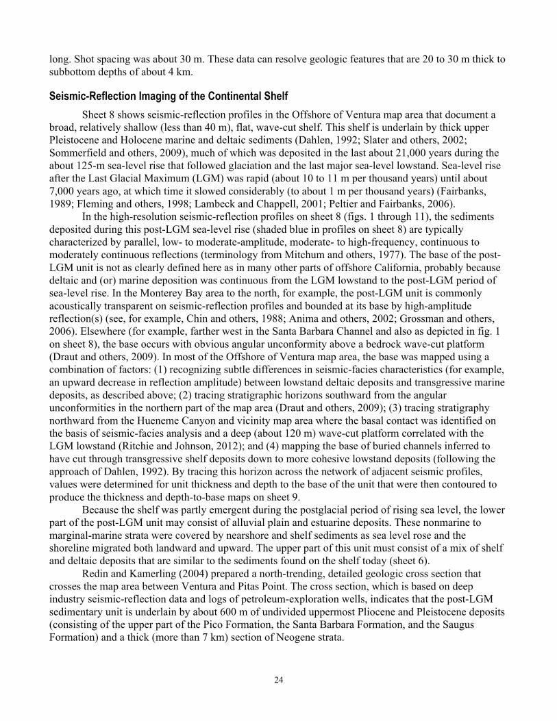
Seismic-Reflection Imaging of the Continental Shelf

Sheet 8 shows seismic-reflection profiles in the Offshore of Ventura map area that document a

broad, relatively shallow (less than 40 m), flat, wave-cut shelf. This shelf is underlain by thick upper

Pleistocene and Holocene marine and deltaic sediments (Dahlen, 1992; Slater and others, 2002;

Sommerfield and others, 2009), much of which was deposited in the last about 21,000 years during the

about 125-m sea-level rise that followed glaciation and the last major sea-level lowstand. Sea-level rise

after the Last Glacial Maximum (LGM) was rapid (about 10 to 11 m per thousand years) until about

7,000 years ago, at which time it slowed considerably (to about 1 m per thousand years) (Fairbanks,

1989; Fleming and others, 1998; Lambeck and Chappell, 2001; Peltier and Fairbanks, 2006).

In the high-resolution seismic-reflection profiles on sheet 8 (figs. 1 through 11), the sediments

deposited during this post-LGM sea-level rise (shaded blue in profiles on sheet 8) are typically

characterized by parallel, low- to moderate-amplitude, moderate- to high-frequency, continuous to

moderately continuous reflections (terminology from Mitchum and others, 1977). The base of the post-

LGM unit is not as clearly defined here as in many other parts of offshore California, probably because

deltaic and (or) marine deposition was continuous from the LGM lowstand to the post-LGM period of

sea-level rise. In the Monterey Bay area to the north, for example, the post-LGM unit is commonly

acoustically transparent on seismic-reflection profiles and bounded at its base by high-amplitude

reflection(s) (see, for example, Chin and others, 1988; Anima and others, 2002; Grossman and others,

2006). Elsewhere (for example, farther west in the Santa Barbara Channel and also as depicted in fig. 1

on sheet 8), the base occurs with obvious angular unconformity above a bedrock wave-cut platform

(Draut and others, 2009). In most of the Offshore of Ventura map area, the base was mapped using a

combination of factors: (1) recognizing subtle differences in seismic-facies characteristics (for example,

an upward decrease in reflection amplitude) between lowstand deltaic deposits and transgressive marine

deposits, as described above; (2) tracing stratigraphic horizons southward from the angular

unconformities in the northern part of the map area (Draut and others, 2009); (3) tracing stratigraphy

northward from the Hueneme Canyon and vicinity map area where the basal contact was identified on

the basis of seismic-facies analysis and a deep (about 120 m) wave-cut platform correlated with the

LGM lowstand (Ritchie and Johnson, 2012); and (4) mapping the base of buried channels inferred to

have cut through transgressive shelf deposits down to more cohesive lowstand deposits (following the

approach of Dahlen, 1992). By tracing this horizon across the network of adjacent seismic profiles,

values were determined for unit thickness and depth to the base of the unit that were then contoured to

produce the thickness and depth-to-base maps on sheet 9.

Because the shelf was partly emergent during the postglacial period of rising sea level, the lower

part of the post-LGM unit may consist of alluvial plain and estuarine deposits. These nonmarine to

marginal-marine strata were covered by nearshore and shelf sediments as sea level rose and the

shoreline migrated both landward and upward. The upper part of this unit must consist of a mix of shelf

and deltaic deposits that are similar to the sediments found on the shelf today (sheet 6).

Redin and Kamerling (2004) prepared a north-trending, detailed geologic cross section that

crosses the map area between Ventura and Pitas Point. The cross section, which is based on deep

industry seismic-reflection data and logs of petroleum-exploration wells, indicates that the post-LGM

sedimentary unit is underlain by about 600 m of undivided uppermost Pliocene and Pleistocene deposits

(consisting of the upper part of the Pico Formation, the Santa Barbara Formation, and the Saugus

Formation) and a thick (more than 7 km) section of Neogene strata.

25

Geologic Structure and Recent Deformation

The Offshore of Ventura map area is cut by two important active faults (sheets 8, 9, 10). The

east-west-striking, south-dipping Oak Ridge Fault (see figs. 7, 8, 10, 11, and 13 on sheet 8) cuts across

the southern part of the map area, and the east-west-striking, north-dipping Pitas Point Fault (see figs.

2, 3, 4, 5, and 9 on sheet 8) cuts across the northern part of the map area. Both faults are part of fault

systems that extend for more than 100 km through the Ventura and Santa Barbara Basins (see, for

example, Sorlien and others, 2000; Fisher and others, 2009). Different models exist for the geometry of

these faults (for example, Shaw and Suppe, 1994; Huftile and Yeats, 1995; Redin and others, 1998;

Yeats, 1998; Sorlien and others, 2000; Redin and Kamerling, 2004; Wills and others, 2008), but they all

concur that the Oak Ridge and Pitas Point Faults are blind-reverse or blind-thrust faults and (or)

components of regional thrust-fault systems.

It is important to note that deformation along both the Pitas Point Fault and the offshore Oak

Ridge Fault is occurring in a dynamic environment that is characterized by abundant sediment supply

from the Santa Clara and Ventura Rivers, as well as active sediment transport. This setting is not

suitable for the formation and preservation of tectonic landforms (for example, scarps, anticlinal ridges),

and evidence of folding and faulting is preserved only once beds are buried below the influence of

surface processes. Nevertheless, the seismic-reflection profiles show fault-related folding (but not

rupture) in the upper stratigraphic unit just a few meters below the seafloor for both the Oak Ridge Fault

and the Pitas Point Fault, indicating Holocene activity. Both high-resolution (for example, fig. 6 on sheet

8) and deeper industry seismic-reflection profiles (figs. 12, 13 on sheet 8) indicate that the area between

the Oak Ridge and Pitas Point Faults is relatively undeformed.

Onland (about 25 km east of Ventura), Yeats and Huftile (1995), Yeats (1998), and Azor and

others (2002) have suggested that the Oak Ridge Fault forms the southern margin of the Ventura Basin

and that it had an early Pleistocene slip rate of 5 mm/yr that decreased to about 1 mm/yr in the last

500,000 years. They have further suggested that slip diminished westward to near zero beneath the

Oxnard plain (alluvial plain of the Santa Clara River) and offshore. Interpretations of offshore seismic-

reflection data by Fisher and others (2005) also suggested no latest Pleistocene and Holocene

deformation along the Oak Ridge Fault, but they did note shallow faulting in these strata along the

Montalvo Fault about 3 km to the south. In contrast, newer seismic-reflection data (for example, Sliter

and others, 2008; see also, figs. 7, 8, and 11 on sheet 8) reveal latest Pleistocene and Holocene folding

along strike with the Oak Ridge Fault (also noted in the offshore by Dahlen, 1992). Reflections within

10 m of the surface on the seismic profile in figure 7 (sheet 8) are clearly folded (dips about 2°; note

vertical exaggeration), with 6 to 7 m of structural relief over a lateral distance of about 120 m. Similarly,

the seismic profile in figure 11 (sheet 8) shows a zone of folded reflections and about 6 to 7 m of

warping along the fold trend, extending to within a few meters of the surface. The nearby seismic profile

in figure 8 (sheet 8) displays a more oblique crossing of the fold trend but also shows deformed

reflection(s) less than 10 m below the surface. These data show vertical deformation along the offshore

Oak Ridge Fault, but this structure may also have a component of left-lateral slip (Sorlien and others,

2000; Fisher and others, 2005) that seismic-reflection data do not reveal.

High-resolution seismic-reflection profiles on sheet 8 similarly reveal asymmetric folding in

post-LGM deposits associated with the blind-reverse Pitas Point Fault (see, for example, figs. 2, 3, 4, 5,

and 9). Folded reflections imaged within this upper stratigraphic unit have as much as 24 m of structural

relief (see figs. 3, 4, and 9), dip as steeply as 13° to 18° (see figs. 3, 4), and commonly extend upward to

the seafloor where they have been truncated by erosion (see figs. 4, 9).

The regional pattern of faults and earthquakes occurring between 1932 and 2010 that have

inferred or measured magnitudes greater than 2.0 are shown on Map C (sheet 9). Although locations

have been provided by the CalTech network since 1932, significantly greater precision began in 1969

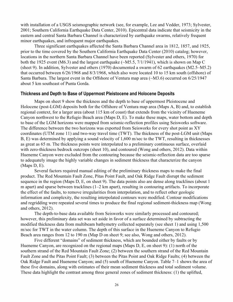
26

with installation of a USGS seismographic network (see, for example, Lee and Vedder, 1973; Sylvester,

2001; Southern California Earthquake Data Center, 2010). Epicentral data indicate that seismicity in the

eastern and central Santa Barbara Channel is characterized by earthquake swarms, relatively frequent

minor earthquakes, and infrequent major earthquakes.

Three significant earthquakes affected the Santa Barbara Channel area in 1812, 1857, and 1925,

prior to the time covered by the Southern California Earthquake Data Center (2010) catalog; however,

locations in the northern Santa Barbara Channel have been reported (Sylvester and others, 1970) for

both the 1925 event (M6.3) and the largest earthquake (~M5.5, 7/1/1941), which is shown on Map C

(sheet 9). In addition, Sylvester and others (1970) documented a swarm of 62 earthquakes (M2.5–M5.2)

that occurred between 6/26/1968 and 8/3/1968, which also were located 10 to 15 km south (offshore) of

Santa Barbara. The largest event in the Offshore of Ventura map area (~M3.6) occurred on 6/25/1947

about 5 km southeast of Punta Gorda.

Thickness and Depth to Base of Uppermost Pleistocene and Holocene Deposits

Maps on sheet 9 show the thickness and the depth to base of uppermost Pleistocene and

Holocene (post-LGM) deposits both for the Offshore of Ventura map area (Maps A, B) and, to establish

regional context, for a larger area (about 115 km of coast) that extends from the vicinity of Hueneme

Canyon northwest to the Refugio Beach area (Maps D, E). To make these maps, water bottom and depth

to base of the LGM horizons were mapped from seismic-reflection profiles using Seisworks software.

The difference between the two horizons was exported from Seisworks for every shot point as XY

coordinates (UTM zone 11) and two-way travel time (TWT). The thickness of the post-LGM unit (Maps

B, E) was determined by applying a sound velocity of 1,600 m/sec to the TWT, resulting in thicknesses

as great as 65 m. The thickness points were interpolated to a preliminary continuous surface, overlaid

with zero-thickness bedrock outcrops (sheet 10), and contoured (Wong and others, 2012). Data within

Hueneme Canyon were excluded from the contouring because the seismic-reflection data are too sparse

to adequately image the highly variable changes in sediment thickness that characterize the canyon

(Maps D, E).

Several factors required manual editing of the preliminary thickness maps to make the final

product. The Red Mountain Fault Zone, Pitas Point Fault, and Oak Ridge Fault disrupt the sediment

sequence in the region (Maps D, E, on sheet 9). The data points also are dense along tracklines (about 1

m apart) and sparse between tracklines (1–2 km apart), resulting in contouring artifacts. To incorporate

the effect of the faults, to remove irregularities from interpolation, and to reflect other geologic

information and complexity, the resulting interpolated contours were modified. Contour modifications

and regridding were repeated several times to produce the final regional sediment-thickness map (Wong

and others, 2012).

The depth-to-base data available from Seisworks were similarly processed and contoured;

however, this preliminary data set was set aside in favor of a surface determined by subtracting the

modified thickness data from multibeam bathymetry collected separately (see sheet 1) and using 1,500

m/sec for TWT in the water column. The depth of this surface in the Hueneme Canyon to Refugio

Beach area ranges from 12 to 190 m (Map D on sheet 9; see also, Wong and others, 2012).

Five different “domains” of sediment thickness, which are bounded either by faults or by

Hueneme Canyon, are recognized on the regional maps (Maps D, E, on sheet 9): (1) north of the

southern strand of the Red Mountain Fault Zone; (2) between the southern strand of the Red Mountain

Fault Zone and the Pitas Point Fault; (3) between the Pitas Point and Oak Ridge Faults; (4) between the

Oak Ridge Fault and Hueneme Canyon; and (5) south of Hueneme Canyon. Table 7–1 shows the area of

these five domains, along with estimates of their mean sediment thickness and total sediment volume.

These data highlight the contrast among three general zones of sediment thickness: (1) the uplifted,

27

sediment-poor Santa Barbara shelf (domain 1; mean sediment thickness of 3.5 m); (2) a transitional zone

(domain 2; mean sediment thickness of 18.0 m); and (3) the subsiding, sediment-rich delta and shelf

offshore of the Ventura and Santa Clara Rivers and Calleguas Creek (domains 3, 4, and 5; mean

sediment thicknesses of 39.3, 38.9, and 28.3 m, respectively).

In the Offshore of Ventura map area, thickness data reveal that the post-LGM section south of

the Oak Ridge Fault is about 38 to 50 m thick, increasing in thickness eastward toward the mouth of the

Santa Clara River. Mean sediment thickness for this area is 43.2 m (table 7–1), increasing abruptly by as

much as 6 to 7 m from south to north across the Oak Ridge Fault.

Post-LGM sediment thickness ranges from about 20 to 50 m between the Pitas Point and Oak

Ridge Faults; the lower values are located offshore of the Ventura River mouth, and the higher values

are located adjacent to the Oak Ridge Fault and also in an oval-shaped area along the southwest edge of

the map area, 1 to 4 km south of the Pitas Point Fault. Mean post-LGM sediment thickness for this area

is 39.2 m (table 7–1). Post-LGM sediment thickness increases by as much as 25 m from north to south

across the Pitas Point Fault.

Post-LGM sediment thickness ranges from 0 to about 35 m north of the Pitas Point Fault, with

the lowest values nearshore and the highest values adjacent to the Pitas Point Fault near the west edge of

the map area. Mean sediment thickness for this area is 17 m, with thickness increasing parallel to the

coast in the nearshore and perpendicular to the coast (and parallel to the Pitas Point Fault) farther

offshore.

Contours on the depth to base of the post-LGM unit generally lie parallel to the shoreline (Map

A, sheet 9). Local, more east-west trends of the contours on this depth surface outline depocenters and

uplifts associated with the Oak Ridge and Pitas Point Faults.

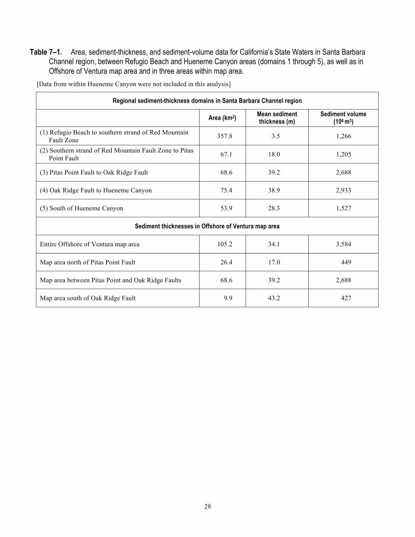
28

Table 7–1. Area, sediment-thickness, and sediment-volume data for California’s State Waters in Santa Barbara Channel region, between Refugio Beach and Hueneme Canyon areas (domains 1 through 5), as well as in

Offshore of Ventura map area and in three areas within map area.

[Data from within Hueneme Canyon were not included in this analysis]

Regional sediment-thickness domains in Santa Barbara Channel region

Area (km2) Mean sediment thickness (m)

Sediment volume (106 m3)

(1) Refugio Beach to southern strand of Red Mountain

Fault Zone 357.8 3.5 1,266

(2) Southern strand of Red Mountain Fault Zone to Pitas

Point Fault 67.1 18.0 1,205

(3) Pitas Point Fault to Oak Ridge Fault 68.6 39.2 2,688

(4) Oak Ridge Fault to Hueneme Canyon 75.4 38.9 2,933

(5) South of Hueneme Canyon 53.9 28.3 1,527

Sediment thicknesses in Offshore of Ventura map area

Entire Offshore of Ventura map area 105.2 34.1 3,584

Map area north of Pitas Point Fault 26.4 17.0 449

Map area between Pitas Point and Oak Ridge Faults 68.6 39.2 2,688

Map area south of Oak Ridge Fault 9.9 43.2 427

29

Chapter 8. Geologic and Geomorphic Map of the Offshore of Ventura Map Area (Sheet 10)


Geologic and Geomorphic Summary

Marine geology and geomorphology was mapped in the Offshore of Ventura map area from

approximate Mean High Water (MHW) to the 3-nautical-mile limit of California’s State Waters. MHW

is defined at an elevation of 1.33 m above the North American Vertical Datum of 1988 (NAVD 88)

(Weber and others, 2005). Offshore geologic units were delineated on the basis of integrated analyses of

adjacent onshore geology with multibeam bathymetry and backscatter imagery (sheets 1, 2, 3), seafloor-

sediment and rock samples (Reid and others, 2006), digital camera and video imagery (sheet 6), and

high-resolution seismic-reflection profiles (sheet 8).

The onshore geology was compiled from Dibblee (1986), Tan and others (2003a,b), and Tan and

Clahan (2004). Unit ages, which are from Tan and others (2003a,b) and Minor and others (2009), reflect

local stratigraphic relations.

The offshore part of the map area largely consists of a relatively shallow (less than 40 m deep),

gently offshore-dipping (less than 1°) shelf underlain by recent marine and deltaic deposits of the Santa

Clara and Ventura Rivers. The mean annual sediment load of these two rivers exceeds 3.25 kilotons per

year (Warrick and Farnsworth, 2009a), and the area is largely part of an extensive Quaternary deltaic

depocenter (Dahlen, 1992; Slater and others, 2002; Sommerfield and others, 2009). Shelf deposits are

primarily sand (unit Qms) at water depths less than about 25 m and, at depths greater than about 25 m,

are more fine-grained sediment (very fine sand, silt, and clay) of unit Qmsf. The boundary between

units Qms and Qmsf is based on observations and extrapolation from sediment sampling (see, for

example, Reid and others, 2006) and camera ground-truth surveying (see sheet 6). Given that this is an

area of abundant sediment supply and active sediment transport (Barnard and others, 2009; Warrick and

Farnsworth, 2009a), it is important to note that the boundary between units Qms and Qmsf should be

considered transitional and approximate and is expected to shift as a result of seasonal- to annual- to

decadal-scale cycles in wave climate, sediment supply, and sediment transport.

Offshore of the mouth of the Ventura River, at water depths of between 20 and 30 m, the sandy

shelf (unit Qms) includes an area of irregular arcuate depressions floored by coarser sediment (coarse

sand and possibly gravel; unit Qmss). Such features have been referred to as “rippled-scour

depressions” (see, for example, Cacchione and others, 1984) or “sorted bedforms” (see, for example,

Goff and others, 2005; Trembanis and Hume, 2011). Although the general area in which unit Qmss

depressions are found is not likely to change substantially, the boundaries of the unit(s), as well as the

locations of individual depressions and their intervening flat sand sheets, likely are ephemeral, changing

during significant storm events.

Coarser grained deposits (unit Qmsc), which are recognized on the basis of high backscatter

(sheet 3), camera observations (sheet 6), and sampling (Reid and others, 2006; Barnard and others,

2009), are found locally in water depths less than about 15 m. These units are concentrated at the mouths

of the Santa Clara and Ventura Rivers and a few smaller coastal watersheds to the northwest, and they

are inferred to represent wave-winnowed lags of deltaic sediment. It is likely that these deposits are

ephemeral and are commonly covered by finer grained sediment. However, a few areas of unit Qmsc

between Ventura and Pitas Point are not obviously tied to coastal watersheds. One large area in

particular is characterized by high rugosity (see Box A on sheet 5) and high backscatter (see sheet 3);

camera ground-truth surveying (see fig. 2 on sheet 6) reveals that this area consists of boulders, cobbles,

gravel, and sand. The area lies immediately offshore of steep slopes underlain by variably consolidated

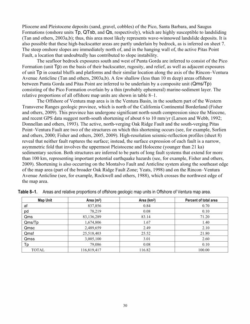
30

Pliocene and Pleistocene deposits (sand, gravel, cobbles) of the Pico, Santa Barbara, and Saugus

Formations (onshore units Tp, QTsb, and Qs, respectively), which are highly susceptible to landsliding

(Tan and others, 2003a,b); thus, this area most likely represents wave-winnowed landslide deposits. It is

also possible that these high-backscatter areas are partly underlain by bedrock, as is inferred on sheet 7.

The steep onshore slopes are immediately north of, and in the hanging wall of, the active Pitas Point

Fault, a location that undoubtedly has contributed to slope instability.

The seafloor bedrock exposures south and west of Punta Gorda are inferred to consist of the Pico

Formation (unit Tp) on the basis of their backscatter, rugosity, and relief, as well as adjacent exposures

of unit Tp in coastal bluffs and platforms and their similar location along the axis of the Rincon–Ventura

Avenue Anticline (Tan and others, 2003a,b). A few shallow (less than 10 m deep) areas offshore

between Punta Gorda and Pitas Point are inferred to be underlain by a composite unit (Qms/Tp)

consisting of the Pico Formation overlain by a thin (probably ephemeral) marine-sediment layer. The

relative proportions of all offshore map units are shown in table 8–1.

The Offshore of Ventura map area is in the Ventura Basin, in the southern part of the Western

Transverse Ranges geologic province, which is north of the California Continental Borderland (Fisher

and others, 2009). This province has undergone significant north-south compression since the Miocene,

and recent GPS data suggest north-south shortening of about 6 to 10 mm/yr (Larson and Webb, 1992;

Donnellan and others, 1993). The active, north-verging Oak Ridge Fault and the south-verging Pitas

Point–Ventura Fault are two of the structures on which this shortening occurs (see, for example, Sorlien

and others, 2000; Fisher and others, 2005, 2009). High-resolution seismic-reflection profiles (sheet 8)

reveal that neither fault ruptures the surface; instead, the surface expression of each fault is a narrow,

asymmetric fold that involves the uppermost Pleistocene and Holocene (younger than 21 ka)

sedimentary section. Both structures are inferred to be parts of long fault systems that extend for more

than 100 km, representing important potential earthquake hazards (see, for example, Fisher and others,

2009). Shortening is also occurring on the Montalvo Fault and Anticline system along the southeast edge

of the map area (part of the broader Oak Ridge Fault Zone; Yeats, 1998) and on the Rincon–Ventura

Avenue Anticline (see, for example, Rockwell and others, 1988), which crosses the northwest edge of

the map area.

Table 8–1. Areas and relative proportions of offshore geologic map units in Offshore of Ventura map area.

Map Unit Area (m2) Area (km2) Percent of total area

af 837,856 0.84 0.70

pd 78,219 0.08 0.10

Qms 83,136,289 83.14 71.20

Qms/Tp 1,674,806 1.67 1.40

Qmsc 2,489,659 2.49 2.10

Qmsf 25,518,403 25.52 21.80

Qmss 3,005,100 3.01 2.60

Tp 79,086 0.08 0.10

TOTAL 116,819,417 116.82 100.00

31

DESCRIPTION OF MAP UNITS

OFFSHORE GEOLOGIC AND GEOMORPHIC UNITS

[Note that, where older units (typically, bedrock) are overlain by thin (<1 m thick) Quaternary deposits,

composite units are mapped. These composite units, which are shown with gray stipple pattern on older

unit, are designated by composite label indicating both overlying sediment cover and lower (older) unit,

separated by slash (for example, Qms/Tp indicates that thin sheet of Qms overlies Tp). Such composite

units are recognized on basis of their high backscatter, flat relief, continuity with moderate- to high-

relief bedrock outcrops, and (in some cases) high-resolution seismic-reflection data. Overlying sediment

is interpreted as ephemeral layer that may or may not be continuously present, whose presence or

absence is function of recency and intensity of storm events, seasonal and (or) annual patterns of

sediment movement, or longer term climate cycles]

af Artificial fill (late Holocene)— Rock, sand, and mud; placed and (or) dredged; includes

coarse construction debris adjacent to Rincon Island (near west edge of map area) and

Ventura Harbor breakwater (fig. 1–2)

pd Platform debris (late Holocene)—Mixed coarse sediment and construction debris

surrounding Rincon Island; includes significant shell debris

Qms Marine nearshore and shelf deposits (late Holocene)—Predominantly sand; ripple marks

common. Found on gently seaward-dipping (less than 1°) surface that extends from

shoreline to water depths of about 25 m

Qmsc Coarse-grained marine nearshore and shelf deposits (late Holocene)—Predominantly

sand to cobbles; found on gently seaward-dipping (less than 1°) surface in water

depths typically less than about 15 m. Recognized primarily on basis of high

backscatter and flat relief. Larger exposures are near mouths of steep coastal

watersheds

Qmsf Fine-grained marine shelf deposits (late Holocene)—Predominantly mud, very fine sand,

and silt; commonly bioturbated; found on gently seaward-dipping (less than 1°)

surface at depths greater than about 25 m in western part of map area

Qmss Marine shelf scour depressions (late Holocene)—Inferred to be coarse sand and possibly

gravel; found as single depressions or in fields of depressions interspersed with

elevated shelf sediments (unit Qms); consists of irregular, arcuate scour depressions

that vary from solitary features occupying a few hundred square meters to two fields

of interconnected depressions covering tens of thousands of square meters.

Depressions, which typically are 15 to 50 cm deep, have diffuse boundaries on

shoreward edge that grade to sharp, well-defined boundaries on offshore edge. In map

area, both backscatter data and direct camera observations (see, for example, figs. 1

and 2 on sheet 4) show small intensity contrasts that suggest that depressions are

filled with sediment that is coarser than intervening elevated sandy shelf deposits.

General area in which unit is found is not likely to change substantially, but

boundaries of unit(s) and locations of individual depressions (and intervening flat

sheets) likely are ephemeral, changing during significant storm events

Tp Pico Formation (Pliocene)—Claystone, siltstone, and sandstone; locally pebbly. Gray-

stippled areas (composite unit Qms/Tp) indicate where thin sheets of Qms overlie

unit

32

ONSHORE GEOLOGIC AND GEOMORPHIC UNITS

[Units are compiled from Dibblee (1986), Tan and others (2003a,b), and Tan and Clahan (2004). Unit

ages, which are from Tan and others (2003a,b) and Minor and others (2009), reflect local stratigraphic

relations]

af Artificial fill (late Holocene)—Engineered and (or) nonengineered

Qb Beach deposits (late Holocene)—Unconsolidated, loose, fine- to coarse-grained sand; well

sorted. Mapped in coastal band from shoreline to highest elevation of swash zone

Qw2 Wash deposits (late Holocene)—Unconsolidated silt, sand, and gravel. Located in major

active river channels

Qe Coastal eolian sand-dune deposits (late Holocene)—Well-sorted, loose sand and silt.

Varies from nonvegetated surfaces that include ephemeral wind ripples to typical

dune-vegetated areas that have thin soil veneers. Mapped in narrow (as wide as 1 km)

coastal strip adjacent to, and above, beach; includes low dunes as tall as 12 m

Qes Coastal-estuarine deposits (late Holocene)—Silty clay. In mud flats that flood during high

tides; also in marshland areas that lie slightly above mean sea level and have brackish

conditions. Deposits have very limited areal extent; mapped only in erosion-protected

areas landward of unit Qe Qf Alluvial fan deposits (late Holocene)—Moderately to poorly bedded sandy clay with some

gravel; deposits originate as debris flows, hyperconcentrated mudflows, or braided

stream flows emanating from mountain canyons

Qw1 Wash deposits (Holocene)—Unconsolidated silt, sand and gravel. Located adjacent to active

channels

Qa Alluvium and colluvium, undivided (Holocene)—Unconsolidated sediment, primarily

sandy clay with some gravel; occurs on valley and canyon floors and includes active

stream deposits in steep areas

Qt Stream-terrace deposits (Holocene)—Unconsolidated, poorly sorted, clayey sand and

sandy clay with gravel; deposited in point-bar and overbank settings; located in

narrow (as wide as 1 km) bands that both flank and are elevated above major active

river channels

Qyf Alluvial fan deposits (Holocene)—Moderately to poorly sorted and bedded gravel, sand,

silt, and clay

Qymp Paralic deposits of Sea Cliff marine terrace (Holocene)—Paralic deposits composed of

semiconsolidated sand and some gravel; 1,800 to 5,800 yr old (Lajoie and others,

1982, 1991)

Qls Landslide deposits and colluvium, undivided (Holocene and Pleistocene)—Disintegrated

bedrock, physically weathered; mapped units range from deep-seated landslides to

active colluvium

Qomp Paralic deposits of Punta Gorda marine terrace (late Pleistocene)—Weakly to

moderately well consolidated, variably stratified, fossiliferous clayey sand, gravel,

and silt; deposited as marine intertidal, beach, and estuarine deposits; forms single

terrace or flights of terraces that range in elevation from 10 to 90 m (30–300 ft) and in

age from 45 ka (oxygen-isotope substage 3a) to 105 ka (substage 5c)

Qoa2 Older alluvial deposits (late and middle Pleistocene)—Silt, sand, clay, and gravel

Qoa1 Older alluvial deposits (middle and early Pleistocene)—Gravel, sand, silt, clay, and

boulders

33

Qc Colluvium (Pleistocene)—Unconsolidated and consolidated silt, sand, clay, and gravel

Qs Saugus Formation (Pleistocene)—Weakly consolidated alluvial deposits, consisting of

sandstone and siliceous-shale gravel and cobbles in sandy matrix

Qlp Las Posas Formation (Pleistocene)—Weakly indurated sand and gravelly sand; highly

susceptible to landsliding

QTsb Santa Barbara Formation (Pleistocene and Pliocene)—Claystone; locally contains shale

fragments of the Monterey Formation

Tp Pico Formation, undivided (Pliocene)—Claystone, siltstone, and sandstone; locally

contains pebbles

Tps Sandstone

Tpsc Sandstone and conglomerate

Tsq Sisquoc Formation (Pliocene and Miocene)—Silty shale; claystone

Tm Monterey Formation, undivided (Miocene)—Siliceous and diatomaceous shale, sandstone,

and limestone

Tmu Upper unit (late Miocene)—Mainly diatomaceous mudstone and shale and subordinate

amounts of dolomite and porcelanite

Tml Lower, calcareous unit (middle and early Miocene)—Calcareous, siliceous, and

phosphatic, white- to tan-weathering mudstone and shale and subordinate amounts of

dolomite, porcelanite, breccia, glauconitic sandstone, and tuff

Tr Rincon Shale (Miocene)—Shale and siltstone

Tv Vaqueros Formation (Miocene)—Sandstone; locally calcareous

Tsp Sespe Formation (Oligocene to late Eocene)—Sandstone, siltstone, and claystone; locally

pebbly

34

Chapter 9. Predictive Distribution of Benthic Macro-Invertebrates for the Offshore of Ventura Map Area and the Santa Barbara Channel Region (Sheet 11)

By Lisa M. Krigsman, Mary M. Yoklavich, Nadine E. Golden, and Guy R. Cochrane

Modeling the distribution of ecologically and economically important species provides managers

and conservation planners with information on a broad spatial scale that is useful to coastal

management, ocean energy, marine protected areas, and marine spatial planning. Sheet 11 displays

predictive models of occurrence for common benthic macro-invertebrate taxa and maps the probability

of occurrence of these taxa in the Santa Barbara Channel region (Krigsman and others, 2012). These

models are based on real-time biological observations of all macro-organisms made during ground-truth

surveys (sheet 6) conducted in 2008 and 2009; the observations were made during a 10-second interval

every minute along video transects, which were approximately 1 km in length (sheet 6; see also, chapter

5 of this pamphlet). These transects produced a total of 923 observations from Refugio Beach (34.5° N.,

120.1° W.) to Hueneme Canyon (34.1° N., 119.2° W.).

Five invertebrate taxa—cup corals, hydroids, short sea pens, tall sea pens, and brittle stars (which

protrude out of the sediment)—were selected for modeling purposes because of their frequent

occurrence in the Santa Barbara Channel; all are structure-forming components of valuable habitat for

groundfish species (Krigsman and others, 2012). Presence-absence data for the selected invertebrates

were fit to multiple generalized linear models using a combination of three covariates—geographic

location, seafloor character (sheet 5), and shaded-relief bathymetry (sheet 2)—as well as relevant

interaction terms. Geographic locations for the five observed invertebrates were derived from analysis of

the video data from an area along the mainland coast of the Santa Barbara Channel; the Offshore of

Carpinteria map area was excluded because of insufficient data. Three statistically different locations

were identified on the basis of a community-structure analysis: (1) the Hueneme Canyon and vicinity

and Offshore of Ventura map areas; (2) the Offshore of Santa Barbara and Offshore of Coal Oil Point

map areas; and (3) the Offshore of Refugio Beach map area. Best-fit models were selected for each

invertebrate on the basis of Akaike’s Information Criterion (AIC) (Akaike, 1974), a best-fit model being

defined as the one that has the fewest parameters within two AIC points of the minimum score.

The seafloor in the Offshore of Ventura map area is predominantly Class I (unconsolidated

sediment), except for a few isolated areas assigned to Class II (mixed habitat) and Class III (rugose rock)

(sheet 5). An extremely low probability of occurrence of cup corals (Map D on sheet 11), a benthic

cnidarian typically found on rocky habitat, exists because the map area is mostly Class I. Even in the

small areas where mixed sediment and rugose rock are present, predictions indicate that cup corals have,

at most, a 50 percent chance of occurrence.

Hydroids (Map C on sheet 11), another benthic cnidarian, have higher predicted probabilities of

occurrence than cup corals. Hydroids commonly are found on habitat similar to cup corals but can also

be found on the surface of unconsolidated sediment. High probabilities of occurrence (about 85 percent)

for hydroids are predicted nearshore on mixed sediment and rugose rock. On unconsolidated sediment,

the probability of occurrence for hydroids increases as depth increases.

Sea pens, also members of the phylum Cnidaria, are divided into two groups—short and tall—on

the basis of their size. Sea pens less than 60 cm in height are identified as short sea pens (Stylatula spp.

and Virgularia spp.); those taller than 60 cm are identified as tall sea pens (Halipteris spp.) (Maps B and

A, respectively, on sheet 11). Sea pens typically are associated with unconsolidated and mixed sediment

because their rootlike base anchors them to the seafloor. Although the seafloor in the Offshore of

Ventura map area is almost completely made up of unconsolidated sediment, the probability of

35

occurrence for either short or tall sea pens is extremely low. A possible explanation for these low

predicted probabilities may be the influence from the outflow of the Santa Clara River, as well as the

impact of wave direction or bottom currents on food availability or sediment characteristics, impinging

their ability to anchor to the seafloor. Bottom-trawling activity in the area may be another explanation.

In the Santa Barbara Channel region, areas where trawling for California halibut (Paralichthys

californicus) takes place coincide with the areas of low predicted occurrence of sea pens (short and tall)

(Frimodig and others, 2008), and such trawling has been reported to have a lasting negative effect on sea

pens (Troffe, 2005; Malecha and Stone, 2009).

Brittle stars in the sediment can occur in such high densities that they create a thick carpet on the

seafloor. Like sea pens, they are typically associated with unconsolidated and mixed sediment into

which they burrow; they also occur in cracks and crevices within rugose rock. As with sea pens, an

extremely low probability (increasing slightly with depth) of brittle star occurrence exists in the

Offshore of Ventura map area (Map E on sheet 11).

Our predictive maps are based on data available from the California Seafloor Mapping Program

(location, habitat type, and bathymetry). Other factors such as ocean currents (Cudaback and others,

2005), water temperature (Bingham and others, 1997), larval distribution (Grantham and others, 2003),

and recruitment and mortality (Keough and Downes, 1982) also can significantly influence the

distribution and abundance of these benthic macro-invertebrate taxa.

36

References Cited

Aikake, H., 1974, A new look at the statistical model identification: Institute of Electrical and

Electronics Engineers Transactions on Automatic Control, v. 19, p. 716–723.

Anderson, T.J., Cochrane, G.R., Roberts, D.A., Chezar, H., and Hatcher, G., 2007, A rapid method to

characterize seabed habitats and associated macro-organisms, in Todd, B.J., and Greene, H.G., eds.,

Mapping the seafloor for habitat characterization: Geological Association of Canada Special Paper 47,

p. 71–79.

Anima, R.J., Eittreim, S.L., Edwards, B.D., and Stevenson, A.J., 2002, Nearshore morphology and late

Quaternary geologic framework of the northern Monterey Bay Marine Sanctuary, California: Marine

Geology, v. 181, p. 35–54.

Azor, A., Keller, E.A., and Yeats, R.S., 2002, Geomorphic indicators of active fold growth, South

Mountain-Oak Ridge anticline, Ventura Basin, southern California: Geological Society of America

Bulletin, v. 114, p. 745–753.

Barnard, P.L., Revell, D.L., Hoover, D., Warrick, J., Brocatus, J., Draut, A.E., Dartnell, P., Elias, E.,

Mustain, N., Hart, P.E., and Ryan, H.F., 2009, Coastal processes study of Santa Barbara and Ventura

counties, California: U.S. Geological Survey Open-File Report 2009–1029, 926 p., available at

http://pubs.usgs.gov/of/2009/1029/.

Bingham, B.L., Bacigalupi, M., and Johnson, L.G., 1997, Temperature adaptations of embryos from

intertidal and subtidal sand dollars (Dendraster excentricus, Eschscholtz): Northwest Science, v.

71(2), p. 108–114.

Briggs, J.C., 1974, Marine zoogeography: New York, McGraw-Hill, 480 p.

Cacchione, D.A., Drake, D.E., Grant, W.D., and Tate, G.B., 1984, Rippled scour depressions of the

inner continental shelf off central California: Journal of Sedimentary Petrology, v. 54, p. 1,280–1,291.

Caldwell, R.J., Taylor, L.A., Eakins, B.W., Carignan, K.S., Grothe, P.R., Lim, E., and Friday, D.Z.,

2010, Digital elevation models of Santa Monica, California—Procedures, data sources and analysis:

NOAA Technical Memorandum NESDIS NGDC-46, NOAA National Geophysical Data Center,

available at http://www.ngdc.noaa.gov/dem/squareCellGrid/download/663.

California Department of Fish and Game, 2008, California Marine Life Protection Act master plan for

marine protected areas—Revised draft: California Department of Fish and Game, accessed April 5,

2011, at http://www.dfg.ca.gov/mlpa/masterplan.asp.

Carignan, K.S., Taylor, L.A., Eakins, B.W., Warnken, R.R., Lim, E., and Medley, P.R., 2009, Digital

elevation model of Santa Barbara, California—Procedures, data sources, and analysis: NOAA

Technical Memorandum NESDIS NGDC-29, NOAA National Geophysical Data Center, available at

http://www.ngdc.noaa.gov/dem/squareCellGrid/download/603.

Chin, J.L., Clifton, H.E., and Mullins, H.T., 1988, Seismic stratigraphy and late Quaternary shelf

history, south-central Monterey Bay, California: Marine Geology, v. 81, p. 137–157.

Cochrane, G.R., 2008, Video-supervised classification of sonar data for mapping seafloor habitat, in

Reynolds, J.R., and Greene, H.G., eds., Marine habitat mapping technology for Alaska: Fairbanks,

University of Alaska, Alaska Sea Grant College Program, p. 185–194, accessed April 5, 2011, at

http://doc.nprb.org/web/research/research%20pubs/615_habitat_mapping_workshop/

Individual%20Chapters%20High-Res/Ch13%20Cochrane.pdf.

Cochrane, G.R., Conrad, J.E., Reid, J.A., Fangman, S., and Golden, N., 2005, Nearshore benthic habitat

GIS for the Channel Islands National Marine Sanctuary and southern California state fisheries

reserves volume II: U.S. Geological Survey Open-File Report 2005–1170, accessed April 5, 2011, at


http://pubs.usgs.gov/of/2009/1029/

http://www.ngdc.noaa.gov/dem/squareCellGrid/download/663

http://www.dfg.ca.gov/mlpa/masterplan.asp

http://www.ngdc.noaa.gov/dem/squareCellGrid/download/603

http://doc.nprb.org/web/research/research%20pubs/615_habitat_mapping_workshop/Individual%20Chapters%20High-Res/Ch13%20Cochrane.pdf


http://doc.nprb.org/web/research/research%20pubs/615_habitat_mapping_workshop/Individual%20Chapters%20High-Res/Ch13%20Cochrane.pdf

37

Cochrane, G.R., and Lafferty, K.D., 2002, Use of acoustic classification of sidescan sonar data for

mapping benthic habitat in the Northern Channel Islands, California: Continental Shelf Research, v.

22, p. 683–690.

Cochrane, G.R., Nasby, N.M., Reid, J.A., Waltenberger, B., and Lee, K.M., 2003, Nearshore benthic

habitat GIS for the Channel Islands National Marine Sanctuary and southern California state fisheries

reserves volume 1: U.S. Geological Survey Open-File Report 03–85, accessed April 5, 2011, at

http://geopubs.wr.usgs.gov/open-file/of03-85/.

Cudaback, C.N., Washburn, L., and Dever, E., 2005, Subtidal inner-shelf circulation near Point

Conception, California: Journal of Geophysical Research, v. 110, C10007,

doi:10.1029/2004JC002608.

Dahlen, M.Z., 1992, Sequence stratigraphy, depositional history, and middle to late Quaternary sea

levels of the Ventura shelf, California: Quaternary Research, v. 38, p. 234–245.

Dartnell, P., Finlayson, D.P., Ritchie, A.C., Cochrane, G.R., and Erdey, M.D., 2012, Bathymetry and

acoustic backscatter—Outer mainland shelf, eastern Santa Barbara Channel, California: U.S.

Geological Survey Data Series 702, 6 p., available at http://pubs.usgs.gov/ds/702/.

Dibblee, T.W., Jr., 1986, Geologic map of the Carpinteria quadrangle, Santa Barbara County, California:

Santa Barbara, Calif., Dibblee Geological Foundation Map DF–04, scale 1:24,000.

Donnellan, A., Hager, B.H., and King, R.W., 1993, Discrepancy between geologic and geodetic

deformation rates in the Ventura basin: Nature, v. 346, p. 333–336.

Draut, A.E., Hart, P.E., Lorenson, T.D., Ryan, H.F., Wong, F.L., Sliter, R.W., and Conrad, J.E., 2009,

Late Pleistocene to Holocene sedimentation and hydrocarbon seeps on the continental shelf of a steep,

tectonically active margin, southern California, USA: Marine Geophysical Research, p. 193–206, doi:

10.1007/s11001-009-9076-y.

Fairbanks, R.G., 1989, A 17,000-year glacio-eustatic sea level record—Influence of glacial melting rates

on the Younger Dryas event and deep-ocean circulation: Science, v. 342, p. 637–642.

Fisher, M.A., Greene, H.G., Normark, W.R., and Sliter, R.W., 2005, Neotectonics of the offshore Oak

Ridge fault near Ventura, southern California: Bulletin of the Seismological Society of America, v. 95,

p. 739–744.

Fisher, M.A., Sorlien, C.C., and Sliter, R.W., 2009, Potential earthquake faults offshore southern

California from the eastern Santa Barbara channel to Dana Point, in Lee, H.J., and Normark, W.R.,

eds., Earth science in the urban ocean—The Southern California Continental Borderland: Geological

Society of America Special Paper 454, p. 271–290.

Fleming, K., Johnston, P., Zwartz, D., Yokoyama, Y., Lambeck, K., and Chappell, J., 1998, Refining the

eustatic sea-level curve since the Last Glacial Maximum using far- and intermediate-field sites: Earth

and Planetary Science Letters, v. 163, p. 327–342, doi:10.1016/S0012-821X(98)00198-8.

Frimodig, A., Horeczko, M., Mason, T., Owens, B., Prall, M., Tillman, T., and Wertz, S., 2008, Review

of California halibut trawl fishery in the California halibut trawl grounds—Report to the California

Fish and Game Commission: California Department of Fish and Game, Marine Region, State

Fisheries Evaluation Project (6/27/2008), 43 p., available at http://www.dfg.ca.gov/marine/sfmp/

halibut-com.asp.

Goff, J.A., Mayer, L.A., Traykovski, P., Buynevich, I., Wilkens, R., Raymond, R., Glang, G., Evans,

R.L., Olson, H., and Jenkins, C., 2005, Detailed investigations of sorted bedforms or “rippled scour

depressions,” within the Martha’s Vineyard Coastal Observatory, Massachusetts: Continental Shelf

Research, v. 25, p. 461–484.

Gotshall, D.W., 2005, Guide to marine invertebrates: Alaska to Baja (2d ed.): Monterey, Calif., Sea

Challengers, 117 p.

Grantham, B.A., Eckert, G.L., and Shanks, A.L., 2003, Dispersal potential of marine invertebrates in

diverse habitats: Ecological Applications, v. 13(1), supplement p. S108–S116.

http://geopubs.wr.usgs.gov/open-file/of03-85/

http://pubs.usgs.gov/ds/702/

http://www.dfg.ca.gov/marine/sfmp/halibut-com.asp

http://www.dfg.ca.gov/marine/sfmp/halibut-com.asp

38

Greene, H.G., Bizzarro, J.J., O’Connell, V.M., and Brylinsky, C.K., 2007, Construction of digital

potential marine benthic habitat maps using a coded classification scheme and its application, in Todd,

B.J., and Greene, H.G., eds., Mapping the seafloor for habitat characterization: Geological Association

of Canada Special Paper 47, p. 141–155.

Greene, H.G., Bizzarro, J.J., Tilden, J.E., Lopez, H.L., and Erdey, M.D., 2005, The benefits and pitfalls

of geographic information systems in marine benthic habitat mapping, in Wright, D.J., and Scholz,

A.J., eds., Place matters: Portland, Oregon State University Press, p. 34–46.

Greene, H.G., Wolf, S.C., and Blom, K.G., 1978, The marine geology of the eastern Santa Barbara

Channel with particular emphasis on the ground water basins offshore from the Oxnard Plain,

southern California: U.S. Geological Survey Open-File Report 78–305, 104 p., 13 plates.

Greene, H.G., Yoklavich, M.M., Starr, R.M., O’Connell, V.M., Wakefield, W.W., Sullivan, D.E.,

McRea, J.E., and Cailliet, G.M., 1999, A classification scheme for deep seafloor habitats:

Oceanologica Acta, v. 22, p. 663–678.

Griggs, G., Patsch, K., and Savoy, L., 2005, Living with the changing California coast: Berkeley,

University of California Press, 540 p.

Grossman, E.E., Eittreim, S.L., Field, M.E., and Wong, F.L., 2006, Shallow stratigraphy and

sedimentation history during high-frequency sea-level changes on the central California shelf:

Continental Shelf Research, v. 26, p. 1,217–1,239.

Hapke, C.J., Reid, D., Richmond, B.B., Ruggiero, P., and List, J., 2006, National assessment of

shoreline change part 3—Historical shoreline change and associated coastal land loss along sandy

shorelines of the California coast: U.S. Geological Survey Open-File Report 2006–1219, 72 p.,

accessed April 5, 2011, at http://pubs.usgs.gov/of/2006/1219/.

Heck, R.G., 1998, Santa Barbara Channel regional formline map, top Monterey Formation, in Kunitomi,

D.S., Hopps, T.E., and Galloway, J.M., eds., Structure and petroleum geology, Santa Barbara Channel,

California: American Association of Petroleum Geologists, Pacific Section, Miscellaneous Publication

46, 1 plate.

Hornafius, J.S., Luyendyk, B.P., Terres, R.R., and Kamerling, M.J., 1986, Timing and extent of

Neogene rotation in the western Transverse Ranges, California: Geological Society of America

Bulletin, v. 97, p. 1,476–1,487.

Huftile, G.J., and Yeats, R.S., 1995, Convergence rates across a displacement transfer zone in the

western Transverse Ranges, Ventura basin, California: Journal of Geophysical Research, v. 100, p.

2,043–2,067.

Jennings, C.W., and Bryant, W.A., 2010, Fault activity map of California: California Geological Survey

Geologic Data Map no. 6, scale 1:750,000.

Keough, M.J., and Downes, B.J., 1982, Recruitment of marine invertebrates—The role of active larval

choices and early mortality: Oecologia, v. 54, 348–352.

Krigsman, L.M., Yoklavich, M.M., Dick, E.J., and Cochrane, G.R., 2012, Models and maps—Predicting

the distribution of corals and other benthic macro-invertebrates in shelf habitats: Ecosphere, v. 3(1),

article 3, 16 p., doi:http://dx.doi.org/10.1890/ES11-00295.1.

Kvitek, R., 2007, California State University, Monterey Bay, Seafloor Mapping Lab Data Library:

California State University, Monterey Bay, Seafloor Mapping Lab database, accessed May 12, 2011,

at http://seafloor.csumb.edu/SFMLwebDATA.htm.

Kvitek, R., Bretz, C., Cochrane, G.R., and Greene, H.G., 2006, Final report, Statewide Marine Mapping

Planning Workshop, December 12–13, 2005, Seaside, Calif.: California State University, Monterey

Bay, 108 p., accessed April 5, 2011, at http://euclase.csumb.edu/DATA_DOWNLOAD/Strategic

MapgWrkshp05/MappingWorkshop12_12-13/Final_Report/CA%20Habitat%20Mapping%20Rpt.pdf.

Kvitek, R.G., Phillips, E.L., and Dartnell, P., 2012, Colored shaded-relief bathymetry, Hueneme Canyon

and vicinity, California, sheet 1 in Johnson, S.Y., Dartnell, P., Cochrane, G.R., Golden, N.E., Phillips,


http://dx.doi.org/10.1890/ES11-00295.1

http://seafloor.csumb.edu/SFMLwebDATA.htm

http://euclase.csumb.edu/DATA_DOWNLOAD/StrategicMapgWrkshp05/MappingWorkshop12_12-13/Final_Report/CA%20Habitat%20Mapping%20Rpt.pdf

http://euclase.csumb.edu/DATA_DOWNLOAD/StrategicMapgWrkshp05/MappingWorkshop12_12-13/Final_Report/CA%20Habitat%20Mapping%20Rpt.pdf

39

E.L., Ritchie, A.C., Kvitek, R.G., Greene, H.G., Krigsman, L.M., Endris, C.A., Clahan, K.B., Sliter,

R.W., Wong, F.L., Yoklavich, M.M., and Normark, W.R. (S.Y. Johnson, ed.), California State Waters

Map Series—Hueneme Canyon and vicinity, California: U.S. Geological Survey Scientific

Investigations Map 3225, pamphlet 41 p., 12 sheets, available at http://pubs.usgs.gov/sim/3225/.

Lajoie, K.R., Ponti, D.J., Powell, C.L., II, Mathieson, S.A., and Sarna-Wojcicki, A.M., 1991, Emergent

marine strandlines and associated sediments, coastal California—A record of Quaternary sea-level

fluctuations, vertical tectonic movements, climatic changes, and coastal processes, in Morrison, R.B.,

ed., The Geology of North America, Quaternary nonglacial geology, conterminous U.S.: Geological

Society of America Decade of North American Geology, v. K-2, p. 190–214.

Lajoie, K.R., Sarna-Wojcicki, A.M., and Yerkes, R.F., 1982, Quaternary chronology and rates of crustal

deformation in the Ventura area, California, in Cooper, J.D., comp., Neotectonics in southern

California: April 1982, 78th Annual Meeting, Geological Society of America Cordilleran Section,

Guidebook, Field Trip 3, p. 43–52.

Lambeck, K., and Chappell, J., 2001, Sea level change through the last glacial cycle: Science, v. 292, p.

679–686, doi: 10.1126/science.1059549.

Larson, K.M., and Webb, F.H., 1992, Deformation in the Santa Barbara Channel from GPS

measurements 1987–1991: Geophysical News Letters, v. 19, p. 1,491–1,494.

Lee, H.J., and Normark, W.R., eds., 2009, Earth science in the urban ocean—The Southern California

Continental Borderland: Geological Society of America Special Paper 454, 481 p.

Lee, W.H.K., and Vedder, J.G., 1973, Recent earthquake activity in the Santa Barbara Channel region:

Bulletin of the Seismological Society of America, v. 63, p. 1,757–1,773.

Luyendyk, B.P., Kamerling, M.J., and Terres, R.R., 1980, Geometric model for Neogene crustal

rotations in southern California: Geological Society of America Bulletin, v. 91, p. 211–217.

Madden, C.J., Goodin, K.L., Allee, R., Finkbeiner, M., and Bamford, D.E., 2008, Draft Coastal and

Marine Ecological Classification Standard: National Oceanic and Atmospheric Administration

(NOAA) and NatureServe, v. III, 77 p.

Malecha, P.W., and Stone, R.P., 2009, Response of the sea whip Halipteris willemoesi to simulated

trawl disturbance and its vulnerability to subsequent predation: Marine Ecology Progress Series, v.

388, p. 197–206.

Minor, S.A., Kellogg, K.S., Stanley, R.G., Gurrola, L.D., Keller, E.A., and Brandt, T.R., 2009, Geologic

map of the Santa Barbara coastal plain area, Santa Barbara County, California: U.S. Geological

Survey Scientific Investigations Map 3001, scale 1:25,000, 1 sheet, pamphlet 38 p., available at

http://pubs.usgs.gov/sim/3001/.

Mitchum, R.M., Jr., Vail, P.R., and Sangree, J.B., 1977, Seismic stratigraphy and global changes of sea

level, part 6—Stratigraphic interpretation of seismic reflection patterns in depositional sequences, in

Payton, C.E., ed., Seismic stratigraphy—Applications to hydrocarbon exploration: Tulsa, Okla.,

American Association of Petroleum Geologists, p. 117–133.

National Oceanic and Atmospheric Administration, 2011, Coastal ifSAR: Digital Coast, NOAA Coastal

Services Center database, accessed April 5, 2011, at http://www.csc.noaa.gov/digitalcoast/.

Nicholson, C., Sorlien, C., Atwater, T., Crowell, J.C., and Luyendyk, B.P., 1994, Microplate capture,

rotation of the western Transverse Ranges, and initiation of the San Andreas transform as a low-angle

fault system: Geology, v. 22, p. 491–495.

Normark, W.R., Piper, D.J.W., Romans, B.W., Covault, J.A., Dartnell, P., and Sliter, R.W., 2009,

Submarine canyon and fan systems of the California Continental Borderland, in Lee, H.J., and

Normark, W.R., eds., Earth science in the urban ocean—The Southern California Continental

Borderland: Geological Society of America Special Paper 454, p. 141–168.

O’Reilly, W.C., and Guza, R.T., 1993, A comparison of spectral wave models in the Southern California

Bight: Coastal Engineering, v. 19, p. 263–282, doi: 10.1016/0378-3839(93)90032-4.



http://www.csc.noaa.gov/digitalcoast/

40

Peltier, W.R., and Fairbanks, R.G., 2006, Global glacial ice volume and Last Glacial Maximum duration

from an extended Barbados sea level record: Quaternary Science Reviews, v. 25, p. 3,322–3,337.

Petersen, M.D., Frankel, A.D., Harmsen, S.C., Mueller, C.S., Haller, K.M., Wheeler, R.L., Wesson,

R.L., Zeng, Y., Boyd, O.S., Perkins, D.M., Luco, N., Field, E.H., Wills, C.J., and Rukstales, K.S.,

2008, Documentation for the 2008 update of the United States National Seismic Hazard Maps: U.S.

Geological Survey Open-File Report 2008–1128, 61 p., accessed April 5, 2011, at


Redin, T., Forman, J., and Kamerling, M.J., 1998, Regional structure section across the eastern Santa

Barbara Channel, from eastern Santa Cruz Island to the Carpinteria area, Santa Ynez Mountains, in

Kunitomi, D.S., Hopps, T.E., and Galloway, J.M., eds., Structure and petroleum geology, Santa

Barbara Channel, California: American Association of Petroleum Geologists, Pacific Section and

Coast Geological Society, Miscellaneous Publication 46, p. 195, 1 sheet.

Redin, T., and Kamerling, M.J., 2004, Santa Barbara Channel structure and correlation sections:

American Association of Petroleum Geologists, Pacific Section, Publication CS 32, 1 sheet.

Reid, J.A., Reid, J.M., Jenkins, C.J., Zimmerman, M., Williams, S.J., and Field, M.E., 2006,

usSEABED—Pacific Coast (California, Oregon, Washington) offshore surficial-sediment data release:

U.S. Geological Survey Data Series 182, available at http://pubs.usgs.gov/ds/2006/182/.

Ritchie, A.C., and Johnson, S.Y., 2012, Detailed geology and geomorphology, Hueneme Canyon,

California, sheet 11 in Johnson, S.Y., Dartnell, P., Cochrane, G.R., Golden, N.E., Phillips, E.L.,

Ritchie, A.C., Kvitek, R.G., Greene, H.G., Krigsman, L.M., Endris, C.A., Clahan, K.B., Sliter, R.W.,

Wong, F.L., Yoklavich, M.M., and Normark, W.R. (S.Y. Johnson, ed.), California State Waters Map

Series—Hueneme Canyon and vicinity, California: U.S. Geological Survey Scientific Investigations

Map 3225, pamphlet 41 p., 12 sheets, available at http://pubs.usgs.gov/sim/3225/.

Rockwell, T.K., Keller, E.A., and Dembroff, G.R., 1988, Quaternary rate of folding of the Ventura

Avenue anticline, western Transverse Ranges, southern California: Geological Society of America

Bulletin, v. 100, p. 850–858.

Shaw, J.H., and Suppe, J., 1994, Active faulting and growth folding in the eastern Santa Barbara

Channel, California: Geological Society of America Bulletin, v. 106, p. 607–626.

Slater, R.A., Gorsline, D.S., Kolpack, R.L., and Shiller, G.I., 2002, Post-glacial sediments of the

California shelf from Cape San Martin to the US-Mexico border: Quaternary International, v. 92, p.

45–61.

Sliter, R.W., Triezenberg, P.J., Hart, P.E., Draut, A.E., Normark, W.R., and Conrad, J.E., 2008, High-

resolution chirp and mini-sparker seismic reflection data from the southern California continental

shelf—Gaviota to Mugu Canyon: U.S. Geological Survey Open-File Report 2008–1246, accessed

April 5, 2011, at http://pubs.usgs.gov/of/2008/1246/.

Sommerfield, C.R., Lee, H.J., and Normark, W.R., 2009, Postglacial sedimentary record of the southern

California continental shelf and slope, Point Conception to Dana Point, in Lee, H.J., and Normark,

W.R., eds., Earth science in the urban ocean—The Southern California Continental Borderland:

Geological Society of America Special Paper 454, p. 89–116.

Sorlien, C.C., Gratier, J.P., Luyendyk, B.P., Hornafius, J.S., and Hopps, T.E., 2000, Map restoration of

folded and faulted late Cenozoic strata across the Oak Ridge fault, onshore and offshore Ventura

basin, California: Geological Society of America Bulletin, v. 112, p. 1,080–1,090.

Southern California Earthquake Data Center, 2010, Southern California Earthquake Catalog: Southern

California Earthquake Data Center database, accessed April 5, 2011, at http://www.data.scec.org/

eq-catalogs/index.html.

Suppe, J., Chou, G.T., and Hook, S.C., 1992, Rates of folding and faulting determined from growth

strata, in McKlay, K.R., ed., Thrust tectonics: London, Chapman and Hall, p. 105–121.


http://pubs.usgs.gov/ds/2006/182/



http://www.data.scec.org/eq-catalogs/index.html

http://www.data.scec.org/eq-catalogs/index.html

41

Sylvester, A.G., 2001, Catalog of Santa Barbara earthquakes—1800 to 1960: University of California, Santa Barbara, database, accessed April 5, 2011, at http://projects.crustal.ucsb.edu/sb_eqs/ SBEQCatlog/SBEQCATINTRO.html.

Sylvester, A.G., Smith, S.S., and Scholz, C.H., 1970, Earthquake swarm in the Santa Barbara Channel, California, 1968: Bulletin of the Seismological Society of America, v. 60, p. 1,047–1,060.

Tan, S.S., and Clahan, K.B., 2004, Geologic map of the White Ledge Peak 7.5´ quadrangle, Santa Barbara and Ventura Counties, California—A digital database: California Geological Survey Preliminary Geologic Map, scale 1:24,000, available at http://www.conservation.ca.gov/cgs/rghm/ rgm/preliminary_geologic_maps.htm.

Tan, S.S., Jones, T.A., and Clahan, K.B., 2003a, Geologic map of the Ventura 7.5´ quadrangle, Ventura County, California—A digital database: California Geological Survey Preliminary Geologic Map, scale 1:24,000, available at http://www.conservation.ca.gov/cgs/rghm/rgm/ preliminary_geologic_maps.htm.

Tan, S.S., Jones, T.A., and Clahan, K.B., 2003b, Geologic map of the Pitas Point 7.5-minute quadrangle, Ventura County, California—A digital database: California Geological Survey Preliminary Geologic Map, scale 1:24,000, available at http://www.conservation.ca.gov/cgs/rghm/rgm/ preliminary_geologic_maps.htm.

Tissot, B.N., Yoklavich, M.M., Love, M.S., York, K., and Amend, M., 2006, Benthic invertebrates that form habitat on deep banks off southern California, with special reference to deep sea coral: Fishery Bulletin, v. 104, p. 167–181.

Trembanis, A.C., and Hume, T.M., 2011, Sorted bedforms on the inner shelf off northeastern New Zealand—Spatiotemporal relationships and potential paleo-environmental implications: Geo-Marine Letters, v. 31, p. 203–214.

Troffe, P.M., Leving, C.D., Piercey, G.B.E., and Keong, V., 2005, Fishing gear effects and ecology of the sea whip (Halipteris willemoesi (Cnidaria: Octocorallia: Pennatulacea)) in British Columbia, Canada—Preliminary observations: Aquatic Conservation, Marine and Freshwater Ecosystems, v. 15, p. 523–533.

U.S. Geological Survey, 2009, National Archive of Marine Seismic Surveys: U.S. Geological Survey database, accessed April 5, 2011, at http://walrus.wr.usgs.gov/NAMSS/.

Warrick, J.A., and Farnsworth, K.L., 2009a, Sources of sediment to the coastal waters of the Southern California Bight, in Lee, H.J., and Normark, W.R., eds., Earth science in the urban ocean—The Southern California Continental Borderland: Geological Society of America Special Paper 454, p. 39–52.

Warrick, J.A., and Farnsworth, K.L., 2009b, Dispersal of river sediment in the southern California Bight, in Lee, H.J., and Normark, W.R., eds., Earth science in the urban ocean—The Southern California Continental Borderland: Geological Society of America Special Paper 454, p. 53–67.

Weber, K.M., List, J.H., and Morgan, K.L., 2005, An operational Mean High Water datum for determination of shoreline position from topographic lidar data: U.S. Geological Survey Open-File Report 2005–1027, accessed April 5, 2011, at http://pubs.usgs.gov/of/2005/1027/.

Wills, C.J., Weldon, R.J., II, and Bryant, W.A., 2008, Appendix A—California fault parameters for the National Seismic Hazard Maps and Working Group on California Earthquake Probabilities 2007: U.S. Geological Survey Open-File Report 2007–1437A, 48 p., available at http://pubs.usgs.gov/of/ 2007/1437/a/.

Wong, F.L., Phillips, E.L., Johnson, S.Y, and Sliter, R.W., 2012, Modeling of depth to base of Last Glacial Maximum and seafloor sediment thickness for the California State Waters Map Series, eastern Santa Barbara Channel, California: U.S. Geological Survey Open-File Report 2012–1161, 16 p., available at http://pubs.usgs.gov/of/2012/1161/.

http://projects.crustal.ucsb.edu/sb_eqs/SBEQCatlog/SBEQCATINTRO.html

http://www.conservation.ca.gov/cgs/rghm/rgm/preliminary_geologic_maps.htm


http://www.conservation.ca.gov/cgs/rghm/rgm/

http://walrus.wr.usgs.gov/NAMSS/


http://pubs.usgs.gov/of/2007/1437/a/


http://projects.crustal.ucsb.edu/sb_eqs/SBEQCatlog/SBEQCATINTRO.html



http://pubs.usgs.gov/of/2007/1437/a/


42

Xu, J.P., and Noble, M.A., 2009, Variability of the southern California wave climate and implications for sediment transport, in Lee, H.J., and Normark, W.R., eds., Earth science in the urban ocean—The Southern California Continental Borderland: Geological Society of America Special Paper 454, p. 171–192.

Yeats, R.S., 1998, North-vergent thick-skinned or south-vergent thin-skinned Oak Ridge fault—A view from the coast, in Kunitomi, D.S., Hopps, T.E., and Galloway, J.M., eds., Structure and petroleum geology, Santa Barbara Channel, California: American Association of Petroleum Geologists, Pacific Section and Coast Geological Society, Miscellaneous Publication 46, p. 143–152.

Yeats, R.S., and Huftile, G.J., 1995, The Oak Ridge fault system and the 1994 Northridge earthquake: Nature, v. 373, p. 418–420.

California State Waters Map Series—Offshore of Ventura, California · Ventura” map area (figs....

Documents

Transcript of California State Waters Map Series—Offshore of Ventura, California · Ventura” map area (figs....