California Investor-Owned Utility Electricity Load Shapes
280
DOCKETED Docket Number: 20-IEPR-03 Project Title: Electricity and Natural Gas TN #: 234507 Document Title: California Investor-Owned Utility Electricity Load Shapes Description: California Energy Commission FINAL PROJECT REPORT CEC-500-2019-046/CEC-500-2019-046 Filer: Raquel Kravitz Organization: California Energy Commission Submitter Role: Commission Staff Submission Date: 8/26/2020 3:48:03 PM Docketed Date: 8/26/2020
Transcript of California Investor-Owned Utility Electricity Load Shapes

DOCKETED Docket Number: 20-IEPR-03
Project Title: Electricity and Natural Gas
TN #: 234507
Document Title: California Investor-Owned Utility Electricity Load Shapes
Description:
California Energy Commission
FINAL PROJECT REPORT
CEC-500-2019-046/CEC-500-2019-046
Filer: Raquel Kravitz
Organization: California Energy Commission
Submitter Role: Commission Staff
Submission Date: 8/26/2020 3:48:03 PM
Docketed Date: 8/26/2020

California Energy Commission
FINAL PROJECT REPORT
California Investor-Owned Utility Electricity Load Shapes
California Energy Commission
Gavin Newsom, Governor
April 2019 | CEC-500-2019-046

PREPARED BY:
DISCLAIMER
This report was prepared as the result of work sponsored by the California Energy Commission. It does
not necessarily represent the views of the Energy Commission, its employees or the State of California.
The Energy Commission, the State of California, its employees, contractors and subcontractors make no
warranty, express or implied, and assume no legal liability for the information in this report; nor does any
party represent that the uses of this information will not infringe upon privately owned rights. This report
has not been approved or disapproved by the California Energy Commission nor has the California Energy
Commission passed upon the accuracy or adequacy of the information in this report.
Primary Author(s):
Sasha Baroiant John Barnes Daniel Chapman Steven Keates Jeffrey Phung ADM Associates, Inc. 3239 Ramos Circle Sacramento, CA 95827 (916) 363-8383 www.admenergy.com Contract Number: 300-15-013
PREPARED FOR: California Energy Commission
Kristen Widdifield Chris Kavalec Anthony Ng Mitch Tian Contract Managers Project Managers
Erik Stokes Matt Coldwell Office Manager Office Manager ENERGY DEPLOYMENT & DEMAND ANALYSIS MARKET FACILITATION OFFICE OFFICE
Laurie ten Hope Deputy Director ENERGY RESEARCH AND DEVELOPMENT DIVISION Siva Gunda Deputy Director ENERGY ASSESSMENTS DIVISION
Drew Bohan Executive Director

i
ACKNOWLEDGEMENTS
The authors feel privileged as beneficiaries of the institutional knowledge of Demand
Analysis Office staff, who provided guidance and perspective during the course of this
project. Andrea Gough helped to identify several existing data sources that avoided or
reduced the scope of data requests to utility companies. Seran Thamilseran provided
key references that described the Forecast Model, along with feedback that put our work
in proper perspective. Mohsen Abrishami provided outputs of the commercial forecast,
and technical feedback on our project framework. Mitch Tian, in addition to reviewing
thousands of load shapes, described the Hourly Electric Load Model (HELM), provided
input and output formats, and helped define the use case for the HELM 2.0 software.
Chris Kavalec provided key guidance on the overall project framework as well as
residential forecast data. Kristen Widdifield provided thorough feedback on this report
and management guidance throughout the project. Lynn Marshall provided time-of-use
rate structure and pricing to enable scenario analysis related to electric vehicle charging.
Aniss Bahreinian, Mark Palmere, and Bob McBride provided electric vehicle charging
forecast data, and also put us in contact with Tom Brotherton of CALSTART, who led us
to several HVIP program participants who provided trending data on bus fleet charging.
Noel Crisostomo provided several references related to electric vehicle charging
infrastructure that helped us to put charging energy use in the same aggregation level
and format as other building end-uses in the forecast model. Jesse Gage provided
supplementary data on electric vehicle saturations. Mehrzad Soltani Nia provided
economic driver data and outputs of the industrial forecast. Siva Gunda put us in touch
with numerous Energy Commission staff with expertise related to this work. Mike Jaske
described committed savings from utility-run energy efficiency programs and provided
associated data. Numerous staff at investor owned utility companies helped to provide
the aggregated customer meter data that were essential to the project – Catherine
Hackney, Cyrus Sorooshian-Tafti, Sotan Im, and others from Southern California Edison;
David Okuni and Tim Vonder from San Diego Gas & Electric; Caroline Francis and
Valerie Winn of Pacific Gas and Electric. This study did not involve any end-use
monitoring. The authors are indebted to policy makers and industry professionals who
conceived, commissioned and conducted extensive end-use monitoring studies, and
made the data available for public use.

ii
PREFACE
The California Energy Commission’s Demand Forecasting Unit maintains forecasting
models used to develop the Energy Commission’s electricity and natural gas demand
forecasts. The electric forecast models’ output expected annual energy usages by
customer sector and geographical zone. The Energy Commission’s Hourly Electric Load
Model (HELM) converts annual energy use forecasts to hourly demand forecasts by
application of appropriate whole-building, end-use, and energy efficiency load shapes.
This project updated the HELM and all of its load profiles by coupling hourly load data
from investor-owned utilities with analytical and engineering simulation methods.
The California Energy Commission’s Energy Research and Development Division
supports energy research and development programs to spur innovation in energy
efficiency, renewable energy and advanced clean generation, energy-related
environmental protection, energy transmission and distribution and transportation.
In 2012, the Electric Program Investment Charge (EPIC) was established by the California
Public Utilities Commission to fund public investments in research to create and
advance new energy solutions, foster regional innovation and bring ideas from the lab to
the marketplace. The California Energy Commission and the state’s three largest
investor-owned utilities—Pacific Gas and Electric Company, San Diego Gas & Electric
Company and Southern California Edison Company—were selected to administer the
EPIC funds and advance novel technologies, tools, and strategies that provide benefits to
their electric ratepayers.
The Energy Commission is committed to ensuring public participation in its research
and development programs that promote greater reliability, lower costs, and increase
safety for the California electric ratepayer and include:
Providing societal benefits.
Reducing greenhouse gas emission in the electricity sector at the lowest possible
cost.
Supporting California’s loading order to meet energy needs first with energy
efficiency and demand response, next with renewable energy (distributed
generation and utility scale), and finally with clean, conventional electricity
supply.
Supporting low-emission vehicles and transportation.
Providing economic development.
Using ratepayer funds efficiently
California Investor-Owned Utility Electricity Load Shapes is the final report under
Contract Number300-15-013 conducted by ADM, Associates, Inc. The information from
this project contributes to the Energy Research and Development Division’s EPIC
Program. For more information about the Energy Research and Development Division,
please visit the Energy Commission’s website at www.energy.ca.gov/research/ or contact
the Energy Commission at 916-327-1551.

iii
ABSTRACT
This project updated traditional end-use load shapes for six energy sectors and
developed photovoltaic system, light-duty electric vehicle, and energy efficiency load
impact profiles, which will be used as inputs for the Demand Analysis Office’s California
Energy Demand Forecast. The California Energy Commission currently uses the Hourly
Electric Load Model to cast annual energy demand forecast elements into hourly
demands, from which projected annual peak loads are forecasted. The Hourly Electric
Load Model includes weather-sensitive and weather-insensitive load shapes at the end-
use, planning area, and forecast zone level for the residential and commercial sectors,
and at the whole-building level for other sectors. The project updated end-use load
shapes by blending publicly available load shapes from market and metering studies
with building simulations in a framework known as EnergyPlus. The project relied on
aggregated interval meter data provided by electric investor-owned utilities to calibrate
energy simulations and to develop models for other sectors.
The load shapes and profiles developed under this project are dynamic entities within
“load shape generators,” which can respond to relevant factors such as calendar data,
weather data, macroeconomic data, and in some cases, price signals from utility time of
use rates. The project also developed software, in the R statistical package, to enable
scenario analysis and replace the current Hourly Electric Load Model.
Keywords: California Energy Commission, forecast, load shapes, energy efficiency load
impact profiles, Hourly Electric Load Model.
Please use the following citation for this report:
Baroiant, Sasha, John Barnes, Daniel Chapman, Steven Keates and Jeffrey Phung (ADM
Associates, Inc.), 2019. California Investor Owned Utility Electricity Load Shapes.
California Energy Commission. Publication Number: CEC-500-2019-046

iv
TABLE OF CONTENTS Page
Acknowledgements .............................................................................................................................. i
Preface ................................................................................................................................................... ii
Abstract ................................................................................................................................................ iii
Table of Contents ............................................................................................................................... iv
List of Figures ...................................................................................................................................viii
List of Tables ...................................................................................................................................... xv
Executive Summary ............................................................................................................................. 1
Introduction ......................................................................................................................................................... 1
Project Purpose ................................................................................................................................................... 1
Project Approach ................................................................................................................................................ 2
Project Results ..................................................................................................................................................... 2
Technology Transfer.......................................................................................................................................... 4
California Benefits .............................................................................................................................................. 5
CHAPTER 1: Introduction .................................................................................................................. 6
Project Goals and Background ..................................................................................................... 6
Project Description ......................................................................................................................... 6
Project Approach ............................................................................................................................. 7
Load Shape Generators ..................................................................................................................................... 7
Secondary Data Sources ................................................................................................................................... 7
Tuning Shapes to AMI Data ............................................................................................................................. 8
Batch Simulations ............................................................................................................................................ 10
Residual Modeling ........................................................................................................................................... 11
Energy Efficiency Load Impact Profiles ..................................................................................................... 12
EV Charging Profiles ....................................................................................................................................... 13
PV Generation Profiles ................................................................................................................................... 14
Weather and Economic Adjustments......................................................................................................... 15
HELM 2.0 ............................................................................................................................................................ 16
Alternate Approaches Considered ........................................................................................... 17
CHAPTER 2: Base Load Shapes: Residential Sector ................................................................... 18
Data Sources .................................................................................................................................. 18
AMI Data ............................................................................................................................................................. 18
Residential Energy Demand Forecast Model............................................................................................ 19
Weather Data .................................................................................................................................................... 20
Load Shapes ...................................................................................................................................................... 20
Source Selection/Weighting Methodology: Internal Loads .................................................. 23

v
Cooking .............................................................................................................................................................. 24
Dishwasher ........................................................................................................................................................ 29
Dryer ................................................................................................................................................................... 34
Freezer ................................................................................................................................................................ 39
Lighting ............................................................................................................................................................... 44
Pool Heater ........................................................................................................................................................ 49
Pool Pump .......................................................................................................................................................... 54
Refrigerator ....................................................................................................................................................... 59
Spa Heater .......................................................................................................................................................... 64
Spa Pump ........................................................................................................................................................... 69
Television ........................................................................................................................................................... 74
Washer ................................................................................................................................................................ 79
Water Heating: Clothes Washer ................................................................................................................... 84
Water Heating: Dishwasher........................................................................................................................... 84
Water Heating: Other ...................................................................................................................................... 84
Miscellaneous ................................................................................................................................................... 94
Cooling ................................................................................................................................................................ 99
Heating ............................................................................................................................................................. 102
Furnace Fan ..................................................................................................................................................... 102
Residual Load Shape .................................................................................................................. 102
CHAPTER 3: Base Load Shapes: Commercial Sector ............................................................... 109
Method and Data Sources ......................................................................................................... 109
Method .............................................................................................................................................................. 109
Data Sources ................................................................................................................................................... 111
Pre-Simulation Modeling ........................................................................................................... 114
Parametric EnergyPlus Models ................................................................................................ 118
Batch Runs Through R/EnergyPlus Integration ................................................................... 119
Calibration for Commercial Models ....................................................................................... 119
Post Calibration Modeling ........................................................................................................ 120
Residual Load Shape .................................................................................................................. 125
Adjustments for Schools/Colleges ......................................................................................... 131
Adjustments to Capture Unique Characteristics by Zone ................................................. 138
CHAPTER 4: Base Load Shapes: Agricultural Sector ............................................................... 145
Regression Modeling.................................................................................................................. 145
Data Sources ................................................................................................................................ 147
AMI Data ........................................................................................................................................................... 147
Holidays............................................................................................................................................................ 149
Weather Data .................................................................................................................................................. 149
CHAPTER 5: Base Load Shapes: Industrial Sector ................................................................... 150

vi
Regression Modeling.................................................................................................................. 151
Data Sources ................................................................................................................................ 153
AMI Data ........................................................................................................................................................... 153
Economic Forecast Data .............................................................................................................................. 155
Holidays............................................................................................................................................................ 155
Weather Data .................................................................................................................................................. 156
CHAPTER 6: Base Load Shapes: Mining and Extraction ......................................................... 157
Regression Modeling.................................................................................................................. 157
Data Sources ................................................................................................................................ 159
AMI Data ........................................................................................................................................................... 160
Economic Forecast Data .............................................................................................................................. 161
Holidays............................................................................................................................................................ 162
Weather Data .................................................................................................................................................. 162
CHAPTER 7: Base Load Shapes: TCU Load Shapes .................................................................. 163
Regression Modeling.................................................................................................................. 163
Data Sources ................................................................................................................................ 165
AMI Data ........................................................................................................................................................... 165
Economic Forecast Data .............................................................................................................................. 167
Holidays............................................................................................................................................................ 167
Weather Data .................................................................................................................................................. 167
CHAPTER 8: Base Load Shapes: Streetlighting ......................................................................... 168
Photocell Load Shape ................................................................................................................. 168
Traffic Lights ............................................................................................................................... 168
Weighting to Represent Nonmetered Streetlighting ........................................................... 168
CHAPTER 9: PV Load Shapes ....................................................................................................... 169
Method .......................................................................................................................................... 169
SAM Modeling and Sensitivity Studies ................................................................................... 169
Data Sources ................................................................................................................................ 169
Time Averaging of PV Output.................................................................................................. 169
CHAPTER 10: EV Charging Load Shapes ................................................................................... 171
Methodology ................................................................................................................................ 171
Data Sources ................................................................................................................................ 171
Single Family Residential Charging Data ................................................................................................ 171
Multifamily Residential Charging Data ................................................................................................... 175
Nonresidential Light Duty Vehicle Charging Data ............................................................................... 176
Municipal Bus Charging Load Shapes ...................................................................................................... 178
Load Shape Specification and Creation ................................................................................. 179
Light Duty Vehicles ....................................................................................................................................... 179

vii
Medium/Heavy Duty Vehicles .................................................................................................................... 179
Modeling Price Response .......................................................................................................... 182
Determination of Default Price Elasticity Factors ................................................................................ 183
Combining and Processing Forecast Elements .................................................................... 185
Output Format ............................................................................................................................ 187
CHAPTER 11: Energy Efficiency Load Impact Profiles .......................................................... 189
Application of Base Load Shapes and Energy Efficiency Load Impact Profiles to
Scenario Analysis ....................................................................................................................... 189
Characterization of Energy Efficiency Load Impact Profiles ............................................ 189
Synchronous Measures ................................................................................................................................ 189
Near Synchronous Measures ...................................................................................................................... 190
Asynchronous Measures.............................................................................................................................. 191
Review of Potential and Goals Study, AAEE, and Committed Savings ............................ 192
Commercial Sector ........................................................................................................................................ 194
Residential Sector .......................................................................................................................................... 197
Other Sectors .................................................................................................................................................. 199
Additional Considerations in Load Impact Profile Selection ............................................................ 199
Development of Energy Efficiency Load Impacts ................................................................ 201
Lighting Occupancy Sensor Load shapes................................................................................................ 202
Application of Energy Efficiency Load Impact Profiles ...................................................... 203
Distribution of Impacts by Building and Zone .................................................................... 206
REFERENCES .................................................................................................................................... 208
ACRONYMS and ABBREVIATIONS .............................................................................................. 210
APPENDIX A: HELM 2.0 Manual ........................................................................................................ 1
Installing the HELM ......................................................................................................................... 1
Running the HELM: Input Data and Formats............................................................................. 2
Input Files ............................................................................................................................................................. 2
Weather Data ....................................................................................................................................................... 3
Economic Descriptors ....................................................................................................................................... 4
Supporting Data .................................................................................................................................................. 5
Output Formats ................................................................................................................................................... 5
Troubleshooting and Support ......................................................................................................................... 6
APPENDIX B: End-Use to Load Shapes Maps ................................................................................. 1
AAEE Map from Potential and Goals Study ................................................................................................. 1
Committed Savings ............................................................................................................................................ 3

viii
LIST OF FIGURES Page
Figure 1: Example Comparison of a Whole Building Load in 2005 vs. 2015-2016 ............... 8
Figure 2: Example of Monthly Energy Usage .............................................................................. 15
Figure 3: Average Daily Load Shape for Residential Customers in 2014 ............................. 19
Figure 4: Comparison of Monthly Energy Usage for Cooking Load Shape Sources ........... 24
Figure 5: Comparison of the Average Daily Weekday Profile in Winter for Cooking ........ 25
Figure 6: Comparison of the Average Daily Weekend Profile in Winter for Cooking ....... 26
Figure 7: Comparison of the Average Daily Weekday Profile in Spring for Cooking ........ 26
Figure 8: Comparison of the Average Daily Weekend Profile in Spring for Cooking ........ 27
Figure 9: Comparison of the Average Daily Weekday Profile in Summer for Cooking ..... 27
Figure 10: Comparison of the Average Daily Weekend Profile in Summer for Cooking .. 28
Figure 11: Comparison of the Average Daily Weekday Profile in Fall for Cooking ........... 28
Figure 12: Comparison of the Average Daily Weekend Profile in Fall for Cooking ........... 29
Figure 13: Comparison of Monthly Energy Usage for Dishwasher Load Shape Sources .. 30
Figure 14: Comparison of the Average Daily Weekday Profile in Winter for Dishwasher 30
Figure 15: Comparison of the Average Daily Weekend Profile in Winter for Dishwasher 31
Figure 16: Comparison of the Average Daily Weekday Profile in Spring for Dishwasher 31
Figure 17: Comparison of the Average Daily Weekend Profile in Spring for Dishwasher 32
Figure 18: Comparison of the Average Daily Weekday Profile in Summer for Dishwasher
............................................................................................................................................................. 32
Figure 19: Comparison of the Average Daily Weekend Profile in Summer for Dishwasher
............................................................................................................................................................. 33
Figure 20: Comparison of the Average Daily Weekday Profile in Fall for Dishwasher ..... 33
Figure 21: Comparison of the Average Daily Weekend Profile in Fall for Dishwasher ..... 34
Figure 22: Comparison of Monthly Energy Usage for Dryer Load Shape Sources ............. 35
Figure 23: Comparison of the Average Daily Weekday Profile in Winter for Dryer .......... 35
Figure 24: Comparison of the Average Daily Weekend Profile in Winter for Dryer .......... 36
Figure 25: Comparison of the Average Daily Weekday Profile in Spring for Dryer ........... 36
Figure 26: Comparison of the Average Daily Weekend Profile in Spring for Dryer .......... 37
Figure 27: Comparison of the Average Daily Weekday Profile in Summer for Dryer ....... 37
Figure 28: Comparison of the Average Daily Weekend Profile in Summer for Dryer ....... 38
Figure 29: Comparison of the Average Daily Weekday Profile in Fall for Dryer ................ 38
Figure 30: Comparison of the Average Daily Weekend Profile in Fall for Dryer ................ 39
Figure 31: Comparison of Monthly Energy Usage for Freezer Load Shape Sources .......... 40
Figure 32: Comparison of the Average Daily Weekday Profile in Winter for Freezer ....... 40
Figure 33: Comparison of the Average Daily Weekend Profile in Winter for Freezer ....... 41
Figure 34: Comparison of the Average Daily Weekday Profile in Spring for Freezer ....... 41
Figure 35: Comparison of the Average Daily Weekend Profile in Spring for Freezer ....... 42
Figure 36: Comparison of the Average Daily Weekday Profile in Summer for Freezer .... 42
Figure 37: Comparison of the Average Daily Weekend Profile in Summer for Freezer .... 43

ix
Figure 38: Comparison of the Average Daily Weekday Profile in Fall for Freezer ............. 43
Figure 39: Comparison of the Average Daily Weekend Profile in Fall for Freezer ............ 44
Figure 40: Comparison of Monthly Energy Usage for Lighting Load Shape Sources ........ 45
Figure 41: Comparison of the Average Daily Weekday Profile in Winter for Lighting ...... 45
Figure 42: Comparison of the Average Daily Weekend Profile in Winter for Lighting ..... 46
Figure 43: Comparison of the Average Daily Weekday Profile in Spring for Lighting ...... 46
Figure 44: Comparison of the Average Daily Weekend Profile in Spring for Lighting ...... 47
Figure 45: Comparison of the Average Daily Weekday Profile in Summer for Lighting .. 47
Figure 46: Comparison of the Average Daily Weekend Profile in Summer for Lighting .. 48
Figure 47: Comparison of the Average Daily Weekday Profile in Fall for Lighting ........... 48
Figure 48: Comparison of the Average Daily Weekend Profile in Fall for Lighting ........... 49
Figure 49: Monthly Energy Usage for Pool Heater Load Shape .............................................. 50
Figure 50: Daily Weekday Profile in Winter for Pool Heater ................................................... 50
Figure 51: Daily Weekend Profile in Winter for Pool Heater ................................................... 51
Figure 52: Daily Weekday Profile in Spring for Pool Heater ................................................... 51
Figure 53: Daily Weekend Profile in Spring for Pool Heater ................................................... 52
Figure 54: Daily Weekday Profile in Summer for Pool Heater ................................................ 52
Figure 55: Daily Weekend Profile in Summer for Pool Heater................................................ 53
Figure 56: Daily Weekday Profile in Fall for Pool Heater ......................................................... 53
Figure 57: Daily Weekend Profile in Fall for Pool Heater ........................................................ 54
Figure 58: Comparison of Monthly Energy Usage for Pool Pump Load Shape Sources .... 55
Figure 59: Comparison of the Average Daily Weekday Profile in Winter for Pool Pump . 55
Figure 60: Comparison of the Average Daily Weekend Profile in Winter for Pool Pump . 56
Figure 61: Comparison of the Average Daily Weekday Profile in Spring for Pool Pump . 56
Figure 62: Comparison of the Average Daily Weekend Profile in Spring for Pool Pump . 57
Figure 63: Comparison of the Average Daily Weekday Profile in Summer for Pool Pump
............................................................................................................................................................. 57
Figure 64: Comparison of the Average Daily Weekend Profile in Summer for Pool Pump
............................................................................................................................................................. 58
Figure 65: Comparison of the Average Daily Weekday Profile in Fall for Pool Pump ....... 58
Figure 66: Comparison of the Average Daily Weekend Profile in Fall for Pool Pump ...... 59
Figure 67: Comparison of Monthly Energy Usage for Refrigerator Load Shape Sources . 60
Figure 68: Comparison of the Average Daily Weekday Profile in Winter for Refrigerator
............................................................................................................................................................. 60
Figure 69: Comparison of the Average Daily Weekend Profile in Winter for Refrigerator
............................................................................................................................................................. 61
Figure 70: Comparison of the Average Daily Weekday Profile in Spring for Refrigerator 61
Figure 71: Comparison of the Average Daily Weekend Profile in Spring for Refrigerator62
Figure 72: Comparison of the Average Daily Weekday Profile in Summer for Refrigerator
............................................................................................................................................................. 62
Figure 73: Comparison of the Average Daily Weekend Profile in Summer for Refrigerator
............................................................................................................................................................. 63

x
Figure 74: Comparison of the Average Daily Weekday Profile in Fall for Refrigerator .... 63
Figure 75: Comparison of the Average Daily Weekend Profile in Fall for Refrigerator .... 64
Figure 76: Monthly Energy Usage for Spa Heater Load Shape ................................................ 65
Figure 77: Daily Weekday Profile in Winter for Spa Heater .................................................... 65
Figure 78: Daily Weekend Profile in Winter for Spa Heater .................................................... 66
Figure 79: Daily Weekday Profile in Spring for Spa Heater ..................................................... 66
Figure 80: Daily Weekend Profile in Spring for Spa Heater .................................................... 67
Figure 81: Daily Weekday Profile in Summer for Spa Heater ................................................. 67
Figure 82: Daily Weekend Profile in Summer for Spa Heater ................................................. 68
Figure 83: Daily Weekday Profile in Fall for Spa Heater .......................................................... 68
Figure 84: Daily Weekend Profile in Fall for Spa Heater .......................................................... 69
Figure 85: Monthly Energy Usage for Spa Pump Load Shape ................................................. 70
Figure 86: Daily Weekday Profile in Winter for Spa Pump ...................................................... 70
Figure 87: Daily Weekend Profile in Winter for Spa Pump ...................................................... 71
Figure 88: Daily Weekday Profile in Spring for Spa Pump ...................................................... 71
Figure 89: Daily Weekend Profile in Spring for Spa Pump ...................................................... 72
Figure 90: Daily Weekday Profile in Summer for Spa Pump ................................................... 72
Figure 91: Daily Weekend Profile in Summer for Spa Pump .................................................. 73
Figure 92: Daily Weekday Profile in Fall for Spa Pump............................................................ 73
Figure 93: Daily Weekend Profile in Fall for Spa Pump ........................................................... 74
Figure 94: Comparison of Monthly Energy Usage for Television Load Shape .................... 75
Figure 95: Comparison of Daily Weekday Profile in Winter for Television ......................... 75
Figure 96: Comparison of Daily Weekend Profile in Winter for Television ......................... 76
Figure 97: Comparison of Daily Weekday Profile in Spring for Television ......................... 76
Figure 98: Comparison of Daily Weekend Profile in Spring for Television ......................... 77
Figure 99: Comparison of Daily Weekday Profile in Summer for Television ...................... 77
Figure 100: Comparison of Daily Weekend Profile in Summer for Television ................... 78
Figure 101: Comparison of Daily Weekday Profile in Fall for Television ............................ 78
Figure 102: Comparison of Daily Weekend Profile in Fall for Television ............................ 79
Figure 103: Comparison of Monthly Energy Usage for Washer Load Shape Sources ........ 80
Figure 104: Comparison of the Average Daily Weekday Profile in Winter for Washer ..... 80
Figure 105: Comparison of the Average Daily Weekend Profile in Winter for Washer .... 81
Figure 106: Comparison of the Average Daily Weekday Profile in Spring for Washer ..... 81
Figure 107: Comparison of the Average Daily Weekend Profile in Spring for Washer ..... 82
Figure 108: Comparison of the Average Daily Weekday Profile in Summer for Washer .. 82
Figure 109: Comparison of the Average Daily Weekend Profile in Summer for Washer . 83
Figure 110: Comparison of the Average Daily Weekday Profile in Fall for Washer .......... 83
Figure 111: Comparison of the Average Daily Weekend Profile in Fall for Washer .......... 84
Figure 112: Comparison of Monthly Energy Usage for Multifamily Water Heater Load
Shape Sources ................................................................................................................................... 85
Figure 113: Comparison of the Average Daily Weekday Profile in Winter for Multifamily
Water Heater ..................................................................................................................................... 86

xi
Figure 114: Comparison of the Average Daily Weekend Profile in Winter for Multifamily
Water Heater ..................................................................................................................................... 86
Figure 115: Comparison of the Average Daily Weekday Profile in Spring for Multifamily
Water Heater ..................................................................................................................................... 87
Figure 116: Comparison of the Average Daily Weekend Profile in Spring for Multifamily
Water Heater ..................................................................................................................................... 87
Figure 117: Comparison of the Average Daily Weekday Profile in Summer for Multifamily
Water Heater ..................................................................................................................................... 88
Figure 118: Comparison of the Average Daily Weekend Profile in Summer for Multifamily
Water Heater ..................................................................................................................................... 88
Figure 119: Comparison of the Average Daily Weekday Profile in Fall for Multifamily
Water Heater ..................................................................................................................................... 89
Figure 120: Comparison of the Average Daily Weekend Profile in Fall for Multifamily
Water Heater ..................................................................................................................................... 89
Figure 121: Comparison of Monthly Energy Usage for Single-Family Water Heater Load
Shape Sources ................................................................................................................................... 90
Figure 122: Comparison of the Average Daily Weekday Profile in Winter for Single-Family
Water Heater ..................................................................................................................................... 90
Figure 123: Comparison of the Average Daily Weekend Profile in Winter for Single-
Family Water Heater ........................................................................................................................ 91
Figure 124: Comparison of the Average Daily Weekday Profile in Spring for Single-Family
Water Heater ..................................................................................................................................... 91
Figure 125: Comparison of the Average Daily Weekend Profile in Spring for Single-Family
Water Heater ..................................................................................................................................... 92
Figure 126: Comparison of the Average Daily Weekday Profile in Summer for Single-
Family Water Heater ........................................................................................................................ 92
Figure 127: Comparison of the Average Daily Weekend Profile in Summer for Single-
Family Water Heater ........................................................................................................................ 93
Figure 128: Comparison of the Average Daily Weekday Profile in Fall for Single-Family
Water Heater ..................................................................................................................................... 93
Figure 129: Comparison of the Average Daily Weekend Profile in Fall for Single-Family
Water Heater ..................................................................................................................................... 94
Figure 130: Comparison of Monthly Energy Usage for Miscellaneous Load Shape Sources
............................................................................................................................................................. 95
Figure 131: Comparison of the Average Daily Weekday Profile in Winter for
Miscellaneous .................................................................................................................................... 95
Figure 132: Comparison of the Average Daily Weekend Profile in Winter for
Miscellaneous .................................................................................................................................... 96
Figure 133: Comparison of the Average Daily Weekday Profile in Spring for
Miscellaneous .................................................................................................................................... 96
Figure 134: Comparison of the Average Daily Weekend Profile in Spring for
Miscellaneous .................................................................................................................................... 97

xii
Figure 135: Comparison of the Average Daily Weekday Profile in Summer for
Miscellaneous .................................................................................................................................... 97
Figure 136: Comparison of the Average Daily Weekend Profile in Summer for
Miscellaneous .................................................................................................................................... 98
Figure 137: Comparison of the Average Daily Weekday Profile in Fall for Miscellaneous
............................................................................................................................................................. 98
Figure 138: Comparison of the Average Daily Weekend Profile in Fall for Miscellaneous
............................................................................................................................................................. 99
Figure 139: Example of Cooling Load Shapes .......................................................................... 101
Figure 140: Example of Heating Load Shapes .......................................................................... 102
Figure 141: Comparison of Monthly Energy Usage With and Without Residual Load Shape
........................................................................................................................................................... 104
Figure 142: Comparison of the Average Daily Weekday Profile With and Without
Residual in Winter .......................................................................................................................... 104
Figure 143: Comparison of the Average Daily Weekend Profile With and Without
Residual in Winter .......................................................................................................................... 105
Figure 144: Comparison of the Average Daily Weekday Profile With and Without
Residual in Spring .......................................................................................................................... 105
Figure 145: Comparison of the Average Daily Weekend Profile With and Without
Residual in Spring .......................................................................................................................... 106
Figure 146: Comparison of the Average Daily Weekday Profile With and Without
Residual in Summer ....................................................................................................................... 106
Figure 147: Comparison of the Average Daily Weekend Profile With and Without
Residual in Summer ....................................................................................................................... 107
Figure 148: Comparison of the Average Daily Weekday Profile With and Without
Residual in Fall ............................................................................................................................... 107
Figure 149: Comparison of the Average Daily Weekend Profile With and Without
Residual in Fall ............................................................................................................................... 108
Figure 150: Average Daily Load Shape for a Building-Type in the Commercial Sector .. 112
Figure 151: Average Daily Load shape for a Building-Type in the Commercial Sector Post-
Aggregation ..................................................................................................................................... 113
Figure 152: Example Comparison of a Whole Building Load in 2005 vs. 2015-2016...... 115
Figure 153: Example of Cooling, Heating, and Ventilation Profiles in Winter .................. 122
Figure 154: Example of Cooling, Heating, and Ventilation Profiles in Spring .................. 123
Figure 155: Example of Cooling, Heating, and Ventilation Profiles in Summer ............... 123
Figure 156: Example of Cooling, Heating, and Ventilation Profiles in Fall ........................ 124
Figure 157: Comparison of Monthly Energy Usage With and Without Residual Load Shape
........................................................................................................................................................... 126
Figure 158: Comparison of the Average Daily Weekday Profile With and Without
Residual in Winter .......................................................................................................................... 127
Figure 159: Comparison of the Average Daily Weekend Profile With and Without
Residual in Winter .......................................................................................................................... 127

xiii
Figure 160: Comparison of the Average Daily Weekday Profile With and Without
Residual in Spring .......................................................................................................................... 128
Figure 161: Comparison of the Average Daily Weekend Profile With and Without
Residual in Spring .......................................................................................................................... 128
Figure 162: Comparison of the Average Daily Weekday Profile With and Without
Residual in Summer ....................................................................................................................... 129
Figure 163: Comparison of the Average Daily Weekend Profile With and Without
Residual in Summer ....................................................................................................................... 129
Figure 164: Comparison of the Average Daily Weekday Profile With and Without
Residual in Fall ............................................................................................................................... 130
Figure 165: Comparison of the Average Daily Weekend Profile With and Without
Residual in Fall ............................................................................................................................... 130
Figure 166: Example of Average Daily GWh by Month in Colleges ..................................... 131
Figure 167: Comparison of Monthly Energy Usage With and Without Scalar Adjustments
........................................................................................................................................................... 133
Figure 168: Average Daily Weekday Profile With and Without Scalar Adjustments in
Winter ............................................................................................................................................... 134
Figure 169: Average Daily Weekend Profile With and Without Scalar Adjustments in
Winter ............................................................................................................................................... 134
Figure 170: Average Daily Weekday Profile With and Without Scalar Adjustments in
Spring ................................................................................................................................................ 135
Figure 171: Average Daily Weekend Profile With and Without Scalar Adjustments in
Spring ................................................................................................................................................ 135
Figure 172: Average Daily Weekday Profile With and Without Scalar Adjustments in
Summer ............................................................................................................................................ 136
Figure 173: Average Daily Weekend Profile With and Without Scalar Adjustments in
Summer ............................................................................................................................................ 136
Figure 174: Average Daily Weekday Profile With and Without Scalar Adjustments in Fall
........................................................................................................................................................... 137
Figure 175: Average Daily Weekend Profile With and Without Scalar Adjustments in Fall
........................................................................................................................................................... 137
Figure 176: Example of Average Daily GWh by Month in Warehouses .............................. 138
Figure 177: Comparison of Monthly Energy Usage With and Without Scalar Adjustments
........................................................................................................................................................... 140
Figure 178: Average Daily Weekday Profile With and Without Scalar Adjustments in
Winter ............................................................................................................................................... 140
Figure 179: Average Daily Weekend Profile With and Without Scalar Adjustments in
Winter ............................................................................................................................................... 141
Figure 180: Average Daily Weekday Profile With and Without Scalar Adjustments in
Spring ................................................................................................................................................ 141
Figure 181: Average Daily Weekend Profile With and Without Scalar Adjustments in
Spring ................................................................................................................................................ 142

xiv
Figure 182: Average Daily Weekday Profile With and Without Scalar Adjustments in
Summer ............................................................................................................................................ 142
Figure 183: Average Daily Weekend Profile With and Without Scalar Adjustments in
Summer ............................................................................................................................................ 143
Figure 184: Average Daily Weekday Profile With and Without Scalar Adjustments in Fall
........................................................................................................................................................... 143
Figure 185: Average Daily Weekend Profile With and Without Scalar Adjustments in Fall
........................................................................................................................................................... 144
Figure 186: Example of Monthly Energy Use in the Agricultural Sector ............................ 146
Figure 187: Example of Average 24-Hour Profiles in the Agricultural Sector .................. 148
Figure 189: Example of Monthly Energy Use in the Industrial Sector ................................ 151
Figure 190: Example of Average 24-Hour Profiles for a Single Facility Type Across User
Groups .............................................................................................................................................. 154
Figure 191: Example of Average 24-Hour Profiles Post-Aggregation ................................. 155
Figure 192: Example of Monthly Energy Usage for All Buildings of a Single Facility-Type
in Mining and Extraction .............................................................................................................. 158
Figure 193: Example of Average 24-Hour Profiles for a Single Mining and Extraction
Facility-Type Across Rate Classes .............................................................................................. 160
Figure 194: Example of Average 24-Hour Profiles for a Single Mining and Extraction
Facility-Type Across Rate Classes Post-Aggregation .............................................................. 161
Figure 195: Example of Monthly Energy Usage for All Buildings of a Single Facility-Type
in TCU ............................................................................................................................................... 164
Figure 196: Example of Average 24-Hour Profiles for a Single TCU Facility-Type Across
Rate Classes ..................................................................................................................................... 166
Figure 197: Example of Average 24-Hour Profiles for a Single TCU Facility-Type Across
Rate Classes Post-Aggregation .................................................................................................... 167
Figure 198: 2017 Summer Weekday Charging Profile by Battery Capacity ....................... 172
Figure 199: 2017 Summer Weekday Charging Demand by Charging Depth..................... 173
Figure 200: 2017 Percent of Daily Energy Usage by Charging Depth ................................. 174
Figure 201: 2017 Comparison of Charging Profiles Developed from the Joint IOU Report
and ChargePoint Data ................................................................................................................... 175
Figure 202: 2017 Charging Profiles for Single Family and Multifamily Homes ............... 176
Figure 203: 2017 Non-residential Weekday Charging Profiles for Three Types of Light
Duty Vehicles .................................................................................................................................. 178
Figure 204: 2018 Weekday Charging Profiles for Municipal Busses and Shuttle Fleets . 179
Figure 205: 2018 Weekday Charging Profiles for Busses and Medium and Heavy-Duty
Vehicles ............................................................................................................................................ 182
Figure 206: Comparison of Summer Weekday Charging Profiles Developed from the
Joint IOU Report and ChargePoint Data .................................................................................... 184
Figure 207: Schematic of EVIL Model ......................................................................................... 185
Figure 208: Comparison of Lighting Load Shape to Energy Efficiency Load Impact Profile
........................................................................................................................................................... 191

xv
Figure 209: Comparison of Lighting Load Shape and Occupancy Sensor Load Impact
Profile ............................................................................................................................................... 192
Figure 210: Total AAEE Energy Savings by Category and Scenario ..................................... 193
Figure 211: Total AAEE Energy Savings by Sector and Scenario, from the 2017 Integrated
Energy Policy Report ..................................................................................................................... 194
Figure 212: AAEE Commercial Energy Savings by End-Use and Scenario .......................... 195
Figure 213: Utility Program Savings by Specific Measure for Major End-Uses in the
Commercial Sector ......................................................................................................................... 196
Figure 214: AAEE Residential Energy Savings by End-Use and Scenario ........................... 197
Figure 215: Savings by Specific Measure for Major End-uses in the Residential Sector . 198
Figure 216: Load Shapes for Residential Window and Insulation Upgrades in Zone 2 .. 202
Figure 217: Residential Lighting Load Shape, Lighting Efficiency Impact Profile, and
Occupancy Sensor Impact Profile ............................................................................................... 203
Figure 218: Schematic of the Process to Conform AAEE Data into the HELM 2.0 Format
........................................................................................................................................................... 206
LIST OF TABLES Page
Table 1: Example of Hour-Matching the 2014-2016 Profile to the 2005 Profile ................ 10
Table 2: Commercial Building-Types ......................................................................................... 110
Table 3: Example of Hour-Matching the 2014-2016 Profile to the 2005 Profile .............. 117
Table 4: Example Parametric Combination Matrix ................................................................. 118
Table 5 – Mapping of 25 NAICS-based industrial classifications to 15 building types. . 150
Table 6: Assignment of Vehicle Ownership Type Classifications to Commercial
Categories Provided by ChargePoint .......................................................................................... 177
Table 7: Listing of Medium and Heavy-Duty Vehicle Classes ............................................... 180
Table 8: Grouping and Load Shape Construction for the Medium and Heavy-Duty Sector
........................................................................................................................................................... 181
Table 9: List of Load Shapes Used to Model Commercial Sector AAEE Savings ............... 197
Table 10: List of Load Shapes Used to Model Residential Sector AAEE Savings .............. 199
Table 11: Measures in the Potential and Goals Study that Account for the Top 95% of
Commercial HVAC Energy Savings ............................................................................................. 200
Table 12: Percent of Overall Commercial HVAC Energy Savings by Candidate Load Shape
........................................................................................................................................................... 200
Table 13: Excerpt of AAEE Spreadsheet from the 2017 IEPR Forecast ............................... 204
Table 14: Load Shape Assignment for Commercial Lighting Codes and Standards ....... 205
Table B-26: Map of Committed Savings Measures from the Potential and Goals Study ..... 3

1
EXECUTIVE SUMMARY
Introduction
The California Energy Commission (Energy Commission) develops the biennial report
the Integrated Energy Policy Report (IEPR), an integrated assessment of major trends and
issues facing California’s energy sector. The IEPR process includes the California Energy
Demand Forecast Model (CED Model), a forecast of electricity and natural gas demand
for California and a number of planning areas and forecast zones within the state. The
CED Model relies on various component models, including the Hourly Electric Load
Model (HELM), used to predict annual peak demand by end-use, sector, and planning
area. HELM’s foundation is based on numerous end-use and whole building hourly load
shapes, which are used to cast annual energy use to total hourly demand for each
forecast year. These load shapes were last updated (partially) in 2002.
Project Purpose
As part of Agreement Number 300-15-013, the Energy Commission contracted with
ADM Associates, Inc. (ADM) to update end-use load shapes, to develop energy efficiency
load impact profiles, and to enable analysis related to various load growth, energy
efficiency, and weather-based scenarios. The load shapes are used by Energy
Commission staff to convert annual energy demand outputs from the California Energy
Demand Forecast Model (CED Model) to hourly and peak electric demand forecasts. The
project achieved following objectives:
The project team updated base end-use load shapes by sourcing available
secondary data and reconciling those shapes with aggregated whole-building
hourly billing data, provided by utility companies.
The team identified and developed key energy efficiency load impact profiles by
using analytical modeling methods and building energy simulations. Energy
efficiency load impact profiles differ from base load shapes because they
account for interactive effects between internal loads and building heating and
cooling systems. They also simulate impacts of controls-related measures that
change the utilization schedule of lighting or cooling.
The team developed additional load profiles to represent electric vehicle
charging, and to enable scenario analysis related to customer price response due
to time-of-use rates.
The team developed additional load profiles to represent photovoltaic
generation in residential and non-residential sectors.
The team developed a software infrastructure to adapt load shapes to particular
scenarios within the CED Model. This software replaces a portion of the
software in the CED Model.

2
Project Approach
The project followed closely the work plan developed by the Energy Commission in
Request for Proposal number 15-322 (2016). The work plan contained the following
elements:
Literature Review
Development of a Research Plan (referred to as the Analytic Framework)
Data Gathering
Baseline Load Shape Development
Energy Efficiency Load Impact Profiles
Scenario Analysis
Documentation, Training, Technology Transfer and Support
At a high level, the project consisted of the following steps:
1. Develop numerous prototypical energy simulation models to describe end-use
energy usage for each market sector and forecasting zone
2. Inform the energy simulation models with the most up-to-date and realistic end-
use energy intensities and schedules, drawing on resources such as utility
interval meter data, the CEUS (Itron, Inc. 2006), the Database for Energy
Efficiency Resources (DEER) (Itron, Inc. 2011), and other primary and secondary
data related to the characterization of electric end-uses
3. Calibrate the energy simulation models to interval meter data from the
representative utility customers
4. Using the calibrated models, simulate energy efficiency measures and technology
changes that are expected to occur under the Energy Commission forecasting
scenarios
5. Regress over the various model runs above to develop “load shape generators”
that can be used to develop energy efficiency impact load shapes and to project
load shapes across time
6. Develop a user interface or software framework through which the load shape
generators can interact with other components of the CED Model
In addition to load shapes and energy efficiency load impact profiles associated with
buildings, ADM also developed load shapes for EV charging and PV generation.
Project Results
The residential sector consists of two main building types: single family and
multifamily. There are 24 end-uses in the residential model, including six weather-
sensitive end-uses, referred to as heating, ventilation, and air conditioning (HVAC). Load
shapes for the six HVAC-related end-uses were generated using utility provided hourly
advanced metering infrastructure (AMI) data and a regression-based method to isolate
typical non-HVAC loads during weekdays and weekends. This non-HVAC load profile

3
was then subtracted from whole-building load profiles on warmer and colder days to
determine cooling and heating load shapes, respectively. A literature review was
conducted to source new profiles for the 18 non-HVAC-related end-uses.
The commercial sector consists of 12 different building types. There are 10 end-uses in
the commercial sector: three HVAC-related and seven non-HVAC-related end-uses. The
three HVAC-related end-uses were generated using building simulation models run in
the EnergyPlus simulation framework, which is a whole building energy simulation
program maintained by the National Renewable Energy Laboratory (NREL) that models
building energy consumption by key end-uses. Because the building models in
EnergyPlus reflect individual buildings while the load shapes reflect aggregates of
buildings, ADM developed a regression-based calibration method in which multiple
simulations were automatically given weights and were thereby aggregated to create
more representative load shapes. New load shapes for non-HVAC end-uses were sourced
from the last California Commercial End-use Survey (CEUS) (Itron, Inc. 2006). These load
shapes were further modified using an hour-matching algorithm intended to modify the
load shapes relative to changes in whole building load between the last CEUS and
current AMI data.
For the residential and commercial sectors, a residual load shape was developed to
capture the systematic differences between the modeled load shapes and the observed
AMI data. Although each load shape is relatively accurate, there may still be systematic
differences at a whole building level that are not captured on an individual end-use
basis. To capture the portion of error that is systematic in nature, for the residential and
commercial sector, ADM modeled the residual between the modeled whole building load
shape and the observed whole building load shape. The portion that could be modeled
systematically was considered an additional end-use hereby known as the residual load
shape, while the remaining error was discarded as random.
Unlike the residential and commercial sectors, load profiles for the agricultural,
industrial, mining and extraction, and TCU sectors are considered at the whole building
level only. For these sectors, the load shapes were modeled via a regression model to
create predictive coefficients that could be used to generate accurate load shapes going
forward. This regression included temporal factors, such as month, weekday, and hour,
as well as other predictors such as cooling degree hours (CDH), economic predictors,
and linear growth terms.
Utilities generally rely on rate tariffs to bill street lighting. Therefore, most street
lighting remains unmonitored. ADM assumed that street lighting could be broken down
into two main components: outdoor lighting fixtures, such as street lamps, and traffic
lights. For the proportion of energy use assumed to be attributable to outdoor lighting,
ADM used daily sunrise and sunset times to develop a load shape that resembles the
daylight-based operation profiles for street lighting. For the proportion of energy usage
assumed to be attributable to traffic lights, ADM assigned a flat load shape.

4
Load shapes for PV generation were generated using the System Advisor Model (SAM)—a
performance and financial simulation model for renewable energy sources, developed
by NREL. For each forecast zone, a prototypical city was selected, and PV shapes were
generated based on several years of historical weather data at different orientations
(North, South, East, and West). The results were then consolidated across years best
capture a typical weather year. Data from the California Solar Initiative (CSI) was used to
aggregate across panel orientations.
Load shapes for light-duty EV charging were created using data from ChargePoint, which
is the world's largest network of EV charging stations. These load shapes were created
to mimic the Energy Commission’s current EV sectors: household vehicles (charging of
residential vehicles at residential and non-residential locations), commercial fleet
vehicles, and government vehicles. To generate load shapes for EV, ADM created a
separate model known as the EV Infrastructure Load Model (EVIL Model). As part of the
EVIL Model, ADM also included price elasticity terms to model the impacts of time of
use (TOU) rates on EV charging.
In addition to the load shapes described above, ADM also developed energy efficiency
load impact profiles based upon a review of the measures included in the last
Additional Achievable Energy Efficiency (AAEE), ADM determined that efficiency
measures for AAEE could be described by a total of 13 efficiency profiles. ADM relied on
EnergyPlus building simulations to generate these efficiency profiles.
Finally, the results of this project culminated in a revised HELM (HELM 2.0), developed
by ADM and to be used by the Energy Commission for future forecasts. The HELM 2.0 is
a collection of data tables and analysis scripts in the R software environment for
statistical computing. The data tables house the regression constants that comprise the
dynamic load shape generators, as well as historical and typical weather data, economic
data such as gross state products for certain industrial sectors, and tables that map
energy efficiency related forecast elements to specific energy efficiency load impact
profiles. The HELM 2.0 accepts data in the format of annual energy demands or annual
energy savings, and distributes these among all hours of the year to produce hourly
energy demands. The hourly results can be viewed and exported at various levels of
detail, ranging from a statewide aggregate down to a specific combination of forecast
zone, customer sector, and end-use.
Technology Transfer
The primary audience for this project is Energy Commission staff. The updated load
shapes and hourly electric load model allows Energy Commission staff to more
accurately produce the Demand Forecast Model which is used by utilities, the California
Public Utilities Commission, and the California Independent System Operator to inform
energy planning and procurement decisions.
The final version of the revised HELM was delivered to the California Energy
Commission in February 2019 and will be used to generate the next Integrated Energy

5
Policy Report. Furthermore, users in the Energy Commission's electrification department
started commissioning the revised HELM as their primary data source for end-use load
shapes. The Energy Commission has also provided energy efficiency load shapes to
public utility companies so that they can use the new load shapes for cost-effectiveness
testing.
The results of the Load Shapes project have also been shared with the Southern
California Public Power Authority (SCPPA), reducing the amount of utility company
resources needed to conduct primary research.
In addition to this final report, information from the Load Shapes project was presented
at a Demand Analysis Working Group meeting on July 12, 2018. Slides from this
meeting are publicly available at the following website:
http://dawg.energy.ca.gov/meetings/dawg-meeting-electric-vehicle-forecasts
California Benefits
DER technology has advanced significantly over the past decade and current load
shapes used to inform the Energy Commission's demand forecast do not account for the
current and future deployment of demand-side innovations. Developing improved load
shapes will provide an accurate assessment of the contributions of clean energy
technologies to reducing peak demand, integrating renewable energy, and maintaining
electricity system reliability as the deployment of clean energy technologies and
strategies increases over time. This information will be used to improve the Energy
Commission's demand forecast and analysis, and identify and target opportunities for
future EPIC research funding to further reduce cost, improve safety, and improve
reliability.
This project can lead to reduced costs by leading to a more accurate demand forecast
for typical usage of appliances and equipment, building type, and implemented demand-
side policies. This can lead to more certainty on base-line end-use consumption and
provide a better input into the CPUC's Long-Term Procurement Planning efforts so that
only the generation that is truly needed, will be planned and procured.
Although the load profiles have been developed primarily for the CED Model, they have
found other beneficial applications. As one example, all California Publicly Owned
Utilities used the load profiles to conduct cost-effectiveness testing and reporting of
their 2018 Energy Efficiency Programs.

6
CHAPTER 1: Introduction
Project Goals and Background The Energy Commission contracted with ADM for electric load shape development,
which will serve as an input for the CED Model. The goals of the project:
Provided load shapes for electric end-uses addressed by the CED Model.
Provided energy efficiency load impact profiles to address how load shapes may
be impacted by upcoming efficiency standards, by market and technology
changes, and by utility-sponsored energy efficiency programs.
Enabled projection of load shapes through 2030, accounting for how changes in
electric energy use will impact the load shapes.
Project Description The project followed closely the work plan developed by the Energy Commission in
Request for Proposal number 15-322 (2016). The work plan has the following elements:
Literature Review.
Development of a Research Plan (referred to as the Analytic Framework).
Data Gathering.
Baseline Load Shape Development.
Energy Efficiency Load Impact Profiles.
Scenario Analysis.
Documentation, Training, Technology Transfer and Support.
At a high level, the team did the following steps:
1. Develop numerous prototypical energy simulation models to describe end-use
energy usage for each market sector and forecasting zone.
2. Inform the energy simulation models with the most up-to-date and realistic
end-use energy intensities and schedules, drawing on resources such as utility
interval meter data, the CEUS (Itron, Inc. 2006), the Database for Energy
Efficiency Resources (DEER) (Itron, Inc. 2011), and other primary and secondary
data related to the characterization of electric end-uses.
3. Calibrate the energy simulation models to interval meter data from the
representative utility customers.
4. Using the calibrated models, simulate energy efficiency measures and
technology changes that are expected to occur under the Energy Commission
forecasting scenarios.

7
5. Regress over the various model runs above to develop “load shape generators”
that can be used to develop energy efficiency impact load shapes and to project
load shapes across time.
6. Develop a user interface or software framework through which the load shape
generators can interact with other components of the CED Model.
In addition to load shapes and energy efficiency load impact profiles associated with
buildings, ADM also developed load shapes for EV charging and PV generation.
Project Approach This section describes the overall approach taken by ADM. Subsequent chapters detail
the methodologies applied to specific project elements.
Load Shape Generators
Most of the load shapes that are available to the industry are static load shapes. These
load shapes are static arrays, typically at hourly resolution. The main disadvantage of
static load shapes is that they represent one specific scenario. For example, the load
shapes from the CEUS (Itron, Inc. 2006) represent loads in one particular year (2002 for
the California IOUs) and a particular weather scenario (actual 2002 weather). In applying
static load shapes, it is important to be careful that all sourced load shapes are (or are
adapted to be) from the same base year and weather scenario. Otherwise, it may be
possible to erroneously sum loads from disparate day types and weather conditions.
Energy Commission forecasters use the HELM to generate load shapes for a given year
and weather scenario. ADM’s approach to this project is similar to the original HELM.
Rather than generating static load shapes, ADM developed and stored regression models
and coefficients, which can be converted to full hourly load shapes when coupled to
data that represent a particular scenario. The scenario specification could be as simple
as specifying a base calendar year, or may require specification of weather data,
macroeconomic data such as gross state product (GSP) for certain industrial sectors, or
even time-of-use utility rate structures and price-elasticity expectations.
Secondary Data Sources
As part of the scope of the project, ADM was tasked with developing new end-use load
shapes for the commercial and residential sectors. The current load shapes used by the
Energy Commission in the HELM were last modified in 2002, based on metering data
originally collected in the late 1980s. End-use monitoring was not within the scope of
the project. Although residential end-uses generally have not significantly changed,
ADM reviewed additional resources to identify potential load shapes based on more
recent data to supplement the existing load shapes.
For the residential sector, the team reviewed the following data sources to identify
prototypical end-use load shapes for use in HELM 2.0:
Energy Demand Forecast Methods Report (Abrishami et al. 2005)

8
Electric Power Research Institute (EPRI) Load Shape Library 4.0 (2016)
DEER (Itron, Inc. 2011)
Energy and Environmental Economics, Inc. (E3) Energy Efficiency Calculator
(2005)
End-use Load Research in the Pacific Northwest: Why Now? (Grist 2016)
Pennsylvania Statewide Act 129: 2014 Commercial & Residential Light Metering
Study (GDS Associates, Inc. et al. 2014)
ADM work products for clients in California, Nevada, and Pennsylvania.
For commercial, ADM reviewed the following data source for use in HELM 2.0:
CEUS (Itron, Inc. 2006)
The results of this review are discussed in further detail in their respective chapters.
Tuning Shapes to AMI Data
One of the key concerns of using secondary sources as the basis for the commercial and
residential load shapes is the potential for underlying changes in behavior or appliance
efficiency that may result in significant changes to the load shapes. Generally, ADM
anticipated this to be a more significant factor in commercial buildings than residential.
Figure 1 provides a hypothetical example of an average daily profile in 2005 compared
to an average daily profile in 2014-2016.
Figure 1: Example Comparison of a Whole Building Load in 2005 vs. 2015-2016
Hypothetical comparison of a daily load shape in a building in 2005 compared to a building in 2014-2016.
Source: ADM Associates, Inc.

9
In general, one can anticipate that the energy use in 2014-2016 has reduced, on average,
due to changes in building code and improved energy efficiency. In addition, the peak of
the curve is not as pronounced in 2014-2016 relative to 2005. One can make this
assumption because the energy efficiency improvements between 2005 and 2014-2016
are likely to be lighting and office equipment-based improvements, which will reduce
the relative impact of lighting compared to the other end-use loads and consequently
minimize interactive effects in HVAC loads.
Therefore, ADM adapted the load shapes from the CEUS (Itron, Inc. 2006) to match
changes in 2014-2016 due to shifts in energy efficiency and to match the load shapes to
the building sub-type from the original building type.
To adapt the load shapes, the researchers used the following approach:
1. For a given building sub-type in a given forecast zone, project analysts selected
the corresponding major building-type end-use load shapes for the same IOU
from the CEUS (Itron, Inc. 2006)—because forecast zones were redesigned
between the time of the last CEUS and present day, were not able map the load
shapes at a more granular, forecast zone resolution.
2. Outdoor lighting load shapes were developed independently based on historical
sunrise/sunset data. Outdoor lighting was then subtracted from the IOU data
based on its relative weight as predicted from the Commercial Building Energy
Demand Forecast Model.
3. After selecting the appropriate load shape, ADM used the annual demand per
end-use for the major building type for that specific forecast zone as predicted
by the Commercial Building Energy Demand Forecast Model to estimate the
relative weight of each end-use load shape for that building type and forecast
zone. The load shapes were then scaled appropriately. Non-HVAC loads were
then aggregated to generate an estimate of the 2014 whole-building load shape
in absentia of HVAC related loads.
4. Both the IOU load shape for 2014 and the CEUS-based load shape were
normalized, and February was isolated as the "base month." This is because
February showed the least amount of weather-dependence upon exploratory
analysis, suggesting a limited impact of HVAC in this month.
5. After isolating t February for the IOU load shape and the CEUS-based load shape,
the project team ran an hour-matching algorithm. This hour-matching algorithm
looked at every hour in the IOU load shape relative to its percent of peak in that
same day and found its closest match in the corresponding weekday types in the
CEUS data. For example, for 1 a.m. Monday, February 3, 2014, the algorithm
looked at all Mondays in the CEUS load shape and found the hour it most closely
resembled across all Mondays of the CEUS load shape.
6. Table 1 provides an example of the algorithm for a sample 24-hour period.
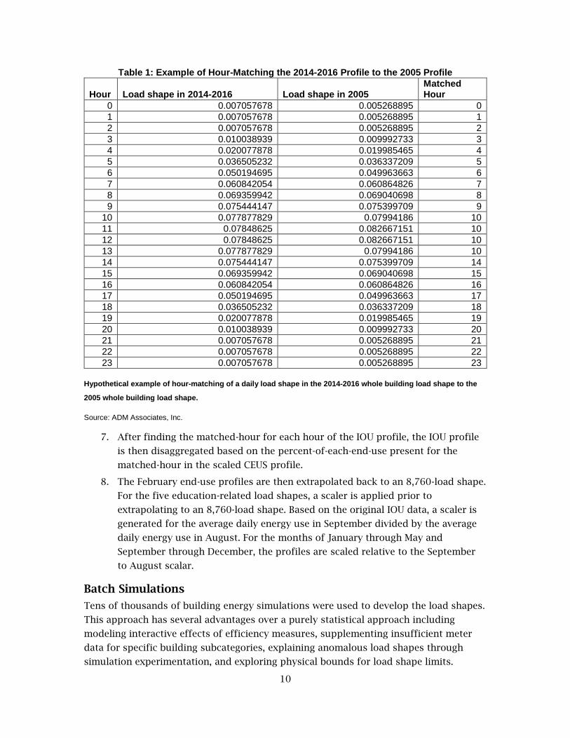
10
Table 1: Example of Hour-Matching the 2014-2016 Profile to the 2005 Profile
Hour Load shape in 2014-2016 Load shape in 2005 Matched Hour
0 0.007057678 0.005268895 0
1 0.007057678 0.005268895 1
2 0.007057678 0.005268895 2
3 0.010038939 0.009992733 3
4 0.020077878 0.019985465 4
5 0.036505232 0.036337209 5
6 0.050194695 0.049963663 6
7 0.060842054 0.060864826 7
8 0.069359942 0.069040698 8
9 0.075444147 0.075399709 9
10 0.077877829 0.07994186 10
11 0.07848625 0.082667151 10
12 0.07848625 0.082667151 10
13 0.077877829 0.07994186 10
14 0.075444147 0.075399709 14
15 0.069359942 0.069040698 15
16 0.060842054 0.060864826 16
17 0.050194695 0.049963663 17
18 0.036505232 0.036337209 18
19 0.020077878 0.019985465 19
20 0.010038939 0.009992733 20
21 0.007057678 0.005268895 21
22 0.007057678 0.005268895 22
23 0.007057678 0.005268895 23
Hypothetical example of hour-matching of a daily load shape in the 2014-2016 whole building load shape to the
2005 whole building load shape.
Source: ADM Associates, Inc.
7. After finding the matched-hour for each hour of the IOU profile, the IOU profile
is then disaggregated based on the percent-of-each-end-use present for the
matched-hour in the scaled CEUS profile.
8. The February end-use profiles are then extrapolated back to an 8,760-load shape.
For the five education-related load shapes, a scaler is applied prior to
extrapolating to an 8,760-load shape. Based on the original IOU data, a scaler is
generated for the average daily energy use in September divided by the average
daily energy use in August. For the months of January through May and
September through December, the profiles are scaled relative to the September
to August scalar.
Batch Simulations
Tens of thousands of building energy simulations were used to develop the load shapes.
This approach has several advantages over a purely statistical approach including
modeling interactive effects of efficiency measures, supplementing insufficient meter
data for specific building subcategories, explaining anomalous load shapes through
simulation experimentation, and exploring physical bounds for load shape limits.

11
The simulations were done using EnergyPlus and controlled with the R programming
language. EnergyPlus was selected because it is highly flexible, well-established
simulation software, and can be run from the command line with manually-controlled
input files. R was used for the data handling and regressions because it is very effective
at statistics at this scale, and it was also used as the scripting language to run
EnergyPlus so that the various R scripts could work together. To complete calculations
of this scale, five dedicated virtual and physical computers were set up to run months of
calculations.
The starting point for the simulation input files were prototypical models taken from
the Institute of Electrical and Electronics Engineers (IEEE), and they were modified to
represent the building types which constituted the subcategories of the study. The
meter data submitted by the IOUs was aggregated from buildings of various sizes,
vintages, HVAC types, envelope parameters, etc., and batches of simulations were
designed to represent the assortment. Statistical techniques were used to select the
weight of each simulation used to find the combination which best matched the meter
data. Early in the program, ADM would need over a hundred simulations per building
type per climate zone, but over time, ADM learned which parameters had the largest
influence on the load shape. ADM learned that setpoint schedules for heating and
cooling were very influential and as ADM sought to drive down uncertainty in the most
challenging shapes, like schools in the summer, setpoint schedules were the best
influence on final load shape.
Dozens of scripts were written to meet the various needs of developing these
simulations. These scripts formatted weather files, modified EnergyPlus input files,
launched batches of simulations, cleaned results, and did other functions.
Residual Modeling
The load shapes developed for the commercial and residential sectors can be described
as either analytically obtained (HVAC load shapes for the residential sector), generated
via an engineering simulation (HVAC load shapes for the commercial sector), or
obtained from the best currently available resources (non-HVAC load shapes). Although,
on an individual basis, each end-use is relatively accurate in nature, there is still
potential for variation between the modeled end-uses and the aggregated data. Because
the data represents an aggregate of all homes belonging to a certain building-
type/forecast zone, it is not readily apparent which specific end-use causes the whole
building load to deviate. It is more likely that the deviation stems from an aggregation
of minor differences between the modeled end-uses and real-world factors.
Therefore, ADM developed a residual load shape. The residual load shape attempts to
recover the component of the residual that is systematic and predictable and acts as a
correction factor that bridges the gap between the modeled whole building load and the
actual whole building load by providing a relative correction to the modeled whole
building. Unlike other load shapes, which are normalized to a total value of one per end-

12
use, the residual load shape is normalized as a percent correction by diving each
observation by the total gigawatt hours (GWh) for the base year for the given building-
type and forecast zone of interest. It can therefore be reconstituted as a function of the
relative intensity of the predicted year by multiplying the normalized profile by the
modeled year's total GWh.
ADM generated the residual load shape by taking the actual residuals (difference
between the actual AMI data and the modeled loads at each hour) and creating a series
of coefficients segmented by time-of-year (month, day-type, and hour) and regressed
against CDH/heating degree hour (HDH) for the commercial sector and cooling degree
day (CDD)/heating degree day (HDD) for the residential sector. To accomplish this, the
analysts first segmented the 8,760 data by its temporal components. For the commercial
sector, the analysts segmented by the data by month, day-type (the seven weekday-types
plus an additional day-type for holidays), and hour. For the Residential sector, the
analysts segmented the data by Pacific Standard Time (PST)/Pacific Daylight Time (PDT),
day-type, and hour.
ADM analysts then ran each segment of data through the following regression model:
𝑦 = 𝛽0 + 𝛽1 ∙ 𝐶𝐷𝐻 + 𝛽2 ∙ 𝐻𝐷𝐻 + 𝜀
Where:
y is the predicted normalized residual
𝛽0 is the intercept
𝛽1 is the CDH weight (CDD for residential)
𝛽2 is the HDH weight (HDD for residential)
𝜀 is the error term
By modeling the residual using this methodology, ADM has captured the variability
remaining that is explainable due to temporal components and weather. The remaining
residuals are discarded as random.
Energy Efficiency Load Impact Profiles
The CED Model includes projections for energy savings associated with energy efficiency
measures. Energy efficiency gains from various sources are considered and included in
the forecast. Energy Commission staff have categorized energy efficiency impacts into
committed energy savings and AAEE. Committed savings are those attributable to
funded, utility-sponsored energy efficiency programs, to approved building standards,
and to approved federal appliance standards. Committed savings are traditionally
included in the baseline forecast. AAEE savings include incremental savings from the
future market potential identified in utility potential studies, but not included in the
baseline demand forecast. AAEE are reasonably expected to occur and include future
updates of building codes, appliance regulations, and new or expanded IOU or publicly-
owned utility (POU) efficiency programs.

13
It is conceptually possible to describe committed savings and AAEE at a high level of
granularity, for example, energy savings by forecast zone, market sector, building or
business type within the market sector, end-use, and specific energy efficiency measure.
For example, one may attempt to forecast all energy savings from anti-sweat heat
controllers in grocery stores in the coastal portion of SDG&E service territory. It is also
possible to develop energy efficiency load impact profiles to couple with specific energy
savings expectation. In practice, however, the level of effort with forecasting energy
savings at such granularity, let alone coupling such forecast elements to appropriate
load impact profiles, would likely be more laborious than the base forecast.
ADM viewed efficiency load impact profile generation and specification as an exercise in
efficiency and restraint as much as a demonstration of the modeling infrastructure’s
capabilities. Rather than generating thousands of energy efficiency load shapes, the
team identified the minimal set of load shapes that have the greatest impact on the
accuracy of AAEE and committed savings hourly demand impacts. The final framework
includes over 1,400 unique energy efficiency load impact profiles, but most of these are
building-type and forecast-zone specific variants of eleven energy efficiency load impact
profiles. In addition to the 11 archetypal energy efficiency load impact profiles, load
shapes are used to characterize energy efficiency savings when appropriate, for
example, outdoor lighting load shapes can be used to characterize load impacts for
outdoor lighting wattage reductions.
The load shapes for the commercial and residential sectors are generally produced by
EnergyPlus models and are then converted to energy efficiency load impact profile
generators through regression modeling. End-use load shapes are not available for
industrial, agricultural, mining, and extraction sectors, and therefore the whole-building
load shape is used as a proxy for AAEE and committed savings for these sectors. This
approach is consistent with present Energy Commission practice for these sectors.
In addition to energy efficiency load impact profile development, the project team has
developed tables that map line items in recent AAEE and committed savings worksheets
used by Energy Commission staff to specific load shapes. ADM has also developed a
means to distribute impacts that are generally at the utility/sector/end-use level of
resolution, to the requisite model format of utility/forecast-zone/sector/building/end-
use/load-shape level. This process is described in Chapter 10.
EV Charging Profiles
Development of load shapes for EV charging was a qualitatively different process than
the rest of the work conducted for the project. EV charging load shape development had
several unique challenges. For example, a representative sample of clean submeter data
for electric vehicle charging is not available from most utility companies. Utility
companies do have data from individually metered chargers for residential customers,
but those customers are generally a minority of the overall customers that are thought
to have electric vehicles. On the other hand, utility companies have demonstrated that

14
TOU rates effectively induce customers to charge during off-peak hours. Given the
expected increased prevalence of TOU rates, historical load shape data may not be
representative of future charging profiles. ADM attempted to obtain recent and
representative data, but to also anticipate the impacts of increased TOU rate
participation. The approach for light duty vehicle charging was to obtain a random
sample of charging session data from ChargePoint, and to build in price elasticity
response with initial elasticity estimates that reconcile the ChargePoint data to data
from pure TOU customers as published in the Joint IOU Electric Vehicle Load Research
Report (SDG&E, SCE and PG&E 2017).
Another challenge with determination of personal light duty vehicle charging is that the
CED Model forecasts EV charging in terms of total charging energy usage for light duty
personal vehicles, yet the rest of the load shape project is in terms of loads at the
customer sector and building type level. Personal electric light duty vehicles are charged
at home (both in single-family and multifamily settings) and at other destinations, such
as workplaces, parking lots, and parking garages. ADM developed tables to disaggregate
personal electric light duty vehicle charging into residential and commercial sectors.
These tables include open parameters for each forecast zone that can be adjusted by
Energy Commission staff as more data becomes available on the charging shares in
single-family, multifamily, and commercial sectors.
Unfortunately, charging data for medium-duty and heavy-duty vehicles is not yet readily
available. ADM was able to obtain trending data, on a voluntary basis, from some
participants of the California Hybrid and Zero Emission Truck and Bus Voucher
Incentive Project (HVIP). These load shapes were primarily for municipal bus fleets and
smaller commercial shuttle fleets. Charging data for several classes of medium and
heavy-duty vehicles are lacking. It is hoped that the recently approved Senate Bill 350
(De León et al. 2015) electrification projects will make available data. ADM decided to
develop several “placeholder” load shapes that may be readily updated as more data
become available.
PV Generation Profiles
ADM used the SAM1 to simulate outputs of solar arrays. The SAM can generate hourly
outputs for numerous market-available systems, in various orientations and
configurations. The output of a particular solar system can depend on various factors,
such as geographical location of installation, orientation (in California, south facing
arrays tend to generate more energy over the year, but west facing arrays have higher
outputs during traditional peak times in late summer afternoons), shading, and tilt.
ADM used data collected from CSI rebate applications to determine the average tilt
angles, and the percentage of panels installed in each orientation. Residential and
1 The SAM is a renewable energy performance and financial model, develop by NREL. The model can be downloaded at https://sam.nrel.gov/.
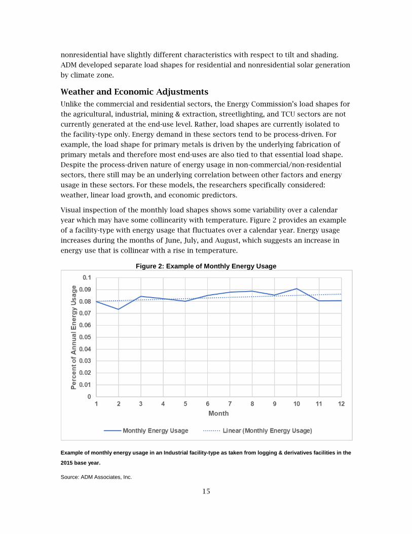
15
nonresidential have slightly different characteristics with respect to tilt and shading.
ADM developed separate load shapes for residential and nonresidential solar generation
by climate zone.
Weather and Economic Adjustments
Unlike the commercial and residential sectors, the Energy Commission’s load shapes for
the agricultural, industrial, mining & extraction, streetlighting, and TCU sectors are not
currently generated at the end-use level. Rather, load shapes are currently isolated to
the facility-type only. Energy demand in these sectors tend to be process-driven. For
example, the load shape for primary metals is driven by the underlying fabrication of
primary metals and therefore most end-uses are also tied to that essential load shape.
Despite the process-driven nature of energy usage in non-commercial/non-residential
sectors, there still may be an underlying correlation between other factors and energy
usage in these sectors. For these models, the researchers specifically considered:
weather, linear load growth, and economic predictors.
Visual inspection of the monthly load shapes shows some variability over a calendar
year which may have some collinearity with temperature. Figure 2 provides an example
of a facility-type with energy usage that fluctuates over a calendar year. Energy usage
increases during the months of June, July, and August, which suggests an increase in
energy use that is collinear with a rise in temperature.
Figure 2: Example of Monthly Energy Usage
Example of monthly energy usage in an Industrial facility-type as taken from logging & derivatives facilities in the
2015 base year.
Source: ADM Associates, Inc.

16
Because of the seasonal nature of energy use, ADM elected to include a temperature-
based term in the regression equation. Although it is unlikely that the increase in energy
usage during the summer is tied specifically to HVAC, CDH can be used to approximate
collinear variables, such as length of day, seasonal production, etc. The researchers
opted to use a CDH term rather than an hourly temperature value to mitigate potential
sensitivity as temperature values reach extreme hot or extreme cold values. Using a CDH
variable ensures that as the temperature dips towards negative values, the term
associated with the weather variable cannot become negative.
ADM also noted significant load growth in the AMI data. As can be seen in Figure 2,
there is a significant linear relationship between monthly energy usage and the number
of months since the origin point (in this case, the origin being January of 2015).
Therefore, the researchers included a “day of year” term (with 1 representing January
1st) in the regression equation to include a term to capture the observed linear growth.
Although the researchers assume that linear growth will continue to be present going
forward, should someone want to exclude linear growth from a generated load shape,
modeling the effect as part of the regression allows one to do so.
In addition to linear load growth and temperature-correlated factors, the project
analysts also reviewed the impact of economic growth or decline on the resulting load
shape. Because production in these sectors are explicitly tied to economic factors, the
researchers felt that changes in the economy could predict changes in the load shape
for one year compared to another. Therefore, the team included historical economic
values as an independent variable in the model. An extract of historical and forecasted
economic data obtained from Moody’s Analytics, Inc.2 was supplied by the California
Energy Commission for the years 2014 through 2028 at a quarterly resolution by North
American Industry Classification System (NAICS) category and forecast zone for the
industrial and mining and extraction sectors. The economic data provided for the
industrial sector were gross GSP values in units of current-day millions of dollars while
the economic data provided for the mining and extraction sector varied between GSP
and employment depending on the facility-type. Economic values were provided for TCU
at an annual basis and varied between employment and population values.
HELM 2.0
HELM 2.0 has many commonalities with the existing HELM. However, the quantity and
types of load shapes differ from those supported by the original HELM, and even
corresponding load shapes have different underlying model structures. ADM decided to
develop a new software to replace the HELM. The HELM 2.0 is developed in the R
statistical programming language. The HELM 2.0 has four major components. The first
2 Moody’s Analytics, Inc. is a financial risk management company which specializes both in business solutions and economic forecasting. For the sake of this project, the data obtained as a pass-through from Moody’s Analytics, Inc. is comprised primarily of economic insight data regarding forecasted employment levels and GSP levels.

17
component is a static database of fixed constants associated with the various load
shapes. The second component includes input data from other components of the CED
Model, as well as scenario-specifics such as weather and economic data. The third
component are files that describe a given scenario list the set of load shapes to be run.
The fourth component is code that reads in parameters and run-specifications, fetches
load shape generator regression coefficients from the database, and performs the
arithmetic requires to generate and summarize full load shapes.
Alternate Approaches Considered The approach to the project follows the analytic framework, developed in December
2016 and revised in March 2017. In the draft framework, the researchers discussed the
following alternate approach to the project. The alternate approach would leverage pre-
existing load shapes for the commercial and residential sector by specifying existing
load shapes from CEUS, DEER, EPRI, and other sources. The advantage of the alternative
approach is that cost savings related to load shape disaggregation and simulation would
allow for primary data collection regarding emerging technologies and electrification in
ports and private and public transportation.
The alternate approach was not selected, in part due to the desire for using recent
interval meter data from IOUs to refresh or validate load shapes, and in part to maintain
focus on scenario analysis capabilities associated with load shape generators. The
project team was able to divert a small portion of the effort to obtain primary and
secondary data related to electric vehicle charging, as described in the approach to
electric vehicle charging profiles.

18
CHAPTER 2: Base Load Shapes: Residential Sector
Data Sources The following section provides a list of the data sources used to generate the residential
load shapes. In addition to listing the data source, a brief description of the data source
and any data preparation activities are provided.
AMI Data
Pacific Gas & Electric, SCE, and SDG&E provided aggregated 15-minute interval meter
data for the years 2014 and 2015 to the Energy Commission as part of the 2017 data
request for the IEPR.3 Data for two of the IOUs was segmented by forecast zone,
building type (multi-family homes versus single-family homes), central space heating
fuel (gas or electric), and use level (high, medium, and low); resulting in 12 sets of
aggregated interval meter data per forecast zone. San Diego Gas & Electric also provided
segmented data but excluded a division between single-family and multi-family homes,
resulting in six sets of aggregated interval meter data per forecast zone. Data was
provided as an averaged load shape, meaning that each observation was an average of
all building types belonging to that categorical segment.
Prior to using the interval meter data, ADM first pre-treated all data. This pre-treatment
consisted of standardizing the nomenclature of all files, converting 15-minute data to
hourly interval meter data, and merging the dataset with climate-zone specific hourly
historical weather data obtained from the Energy Commission. Hourly timestamps were
standardized to units of PST for the entire year (specifically 11 p.m. PDT was
standardized to 10 p.m. PST). Data was restricted to the period of January 1, 2014
through December 31, 2015.
Exploratory analysis on the AMI data showed potential conflation between electric-
heated and gas-heated homes. Specifically, the datasets that were labeled as gas-heated
showed were not distinctly different from electric-heated homes. ADM attributes this
potential conflation as an overstating of homes that have gas-fuel potential with homes
that actively use gas as a fuel source. Furthermore, load shapes did not appear to vary
by usage level post-normalization. Given the similarity of the different types of profiles
and that the end-uses sources via the meta-analysis did not make a distinction amongst
heat fuel or use level, ADM aggregated across the different strata to create one
consolidated profile per forecast zone.
3 Aniss Bahreinian et al. 2017 Integrated Energy Policy Report (2017).

19
Figure 3 provides an example of an average 24-hour load shape taken from a single
forecast zone and building type after the load shapes have been normalized taken
across the entirety of 2014. There is high correspondence between all profiles, thereby
suggesting that neither heat fuel nor usage level play a significant role in the residential
load shape.
Figure 3: Average Daily Load Shape for Residential Customers in 2014
Example of the average daily load shape for all fuel types and energy usage levels for residential customers in a
single forecast zone and building type in 2014.
Source: ADM Associates, Inc.
Furthermore, ADM leveraged electric end-use intensities (EUIs), unit energy
consumptions (UECs), and forecasted sector-wide electric energy consumption per
forecast zone obtained from the CED Model. These values are predicted at a forecast
zone level by building type, but not by usage-level. To bridge the relationship between
the forecast model and the load shape data, ADM aggregated the IOU data across the
three usage levels and scaled the profile to the predicted GWh (exclusive of GWh
attributable to PV generation) from the forecast model.
Residential Energy Demand Forecast Model
The Residential Energy Demand Forecast Model is a component of the CED Model which
predicts the overall annual energy use for a given end-use at either the forecast zone
level (specifically for HVAC end-uses) or at the IOU level (non-HVAC end-uses). The
predicted GWh is further subdivided by building type (single family, multifamily, or

20
mobile home). For example, the summary model has predictions of the total annual
lighting GWh for all single-family residential buildings in SDG&E service territory, or all
single-family cooling for residential buildings in forecast zone 12, etc. Updates are made
to the forecast model on an annual basis, with major revisions occurring bi-annually.
The Energy Commission corrects its historical load forecast based on observed whole-
building energy use on an annual basis, thereby adjusting the end-use level forecast
based on the total observed load.
As part of the process of developing load shapes for the base years of 2014 and 2015,
ADM leveraged the corrected forecast values for 2014 and 2015 and assumed that the
overall energy usage per end-use was distributed in the same proportions as the
Residential Energy Demand Forecast Model. Because ADM was interested in the relative
percent electric distribution by forecast zone, ADM estimated the total GWh attributed
to each forecast zone for non-HVAC end-uses based on population estimates reported
as part of the Residential Energy Demand Forecast Model.
Weather Data
An extract of weather data obtained was supplied by the Energy Commission for the
years 2014 through 2016. Weather data consisted of outdoor air temperature, dew
point, precipitation, windspeed, wind direction, total sky cover, and mean sea level
pressure. Weather files were generated for all major airport weather stations (AWS) in
California. The Energy Commission provided weighting files meant to define the
appropriate weighting of each AWS to generate a forecast-zone-level weather file.
Load Shapes
The current load shapes used by the Energy Commission in HELM were last modified in
2002, based on metering data originally collected in the late 1980s. Although the team
did not anticipate significant changes in the end-use profile, the team reviewed
additional resources to identify potential load shapes based on more recent data to
supplement the existing load shapes. The team reviewed the following data sources to
identify prototypical end-use load shapes for use in HELM 2.0:
Energy Demand Forecast Methods Report (Abrishami et al. 2005)
Electric Power Research Institute (EPRI) Load Shape Library 4.0 (2016)
DEER (Itron, Inc. 2011)
Energy and Environmental Economics, Inc. (E3) Energy Efficiency Calculator
(2005)
End-use Load Research in the Pacific Northwest: Why Now? (Grist 2016)
Pennsylvania Statewide Act 129: 2014 Commercial & Residential Light Metering
Study (GDS Associates, Inc. et al. 2014)
ADM work products for clients in California, Nevada, and Pennsylvania.

21
Current Load Shapes
The team reviewed the load shapes used in the Energy Commission's current version of
HELM. These load shapes were originally developed in the early 1990s based on
metering data from the late 1980s. The load shapes were updated in 2002 by Primen.
The current version of the load shape model relies on end-use coefficients that are
stored at a monthly by weekday type (weekday or weekend) by hour resolution and then
expanded to an 8760-level depending on the calendar year of interest. The coefficients
are static - meaning they do not currently interact with any additional inputs such as
weather. Internal load shapes are currently the same across forecast zones, while HVAC-
related load shapes are different from forecast zone to forecast zone.
The Energy Commission's load shapes do not currently include lighting as one of its
current end-uses. As part of ADM's discussions with the Energy Commission, legacy
waterbed heater end-use will be depreciated and include a lighting end-use in its place.
Load shapes for solar pool pumps, solar water heat - back-up, and solar water heat -
pumps are currently flat 8,760 placeholders.
EPRI Load Shape Library 4.0 (2016)
The Load Shape Library 4.0 is a resource developed by the EPRI and publicly available
online. The database provides aggregated data from regional utility studies, EPRI
proprietary field data, and EPRI CEED (Center for End-Use Energy Data) PowerShapeTM
(2000-2001) data. Residential end-use load shape data is presented by North American
Electric Reliability Corporation (NERC) region, with the most granular region-specific
resolution available being for an aggregated California/Nevada region.
The following non-HVAC residential end-use load shapes are represented in the
database:
Clothes dryer
Clothes washer
Dishwasher
Lighting
Refrigerator
Television (TV) & personal computer (PC)
Water heating
Although some end-use load shapes are available at a region-specific level, several of the
above profiles are only presented across all regions. These end-uses include lighting,
refrigerators, and TV & PC. Furthermore, all end-uses have been reduced to 24-hour
profiles for six day-types:
Peak season, peak weekday
Peak season, average Weekday
Peak season, average Weekend

22
Off peak season, peak weekday
Off peak season, average weekday
Off peak season, average weekend
DEER (Itron, Inc. 2011)
The DEER is a resource developed by the California Public Utilities Commission (CPUC)
to provide information regarding cost, benefit, and ex ante savings for energy efficient
measures. Information provided in DEER is gathered from various work papers from the
three California electric IOUs (PG&E, SDG&E and SCE).
In 2012, the CPUC made electric savings curved for energy efficiency measures covered
by the DEER publicly available for the model year 2013 (DEER 2011). Although these
profiles represent efficiency profile, the corresponding end-use load shapes have similar
shapes to these efficiency profiles.
There are eight non-HVAC efficiency measures represented in the DEER 2011. The three
following items were selected for inclusion as part of the HELM 2.0.:
Refrigerator/freezer recycling - all space types
Dishwashers
Clothes washers
E3 Energy Efficiency Calculator (2005)
The Energy Efficiency Calculator is a resource developed by E3 as an avoided cost tool
for the three California IOUs in response to CPUC proceeding R.04-04-025. The original
version of the E3 Energy Efficiency Calculator relies on load shapes derived from a 1994
metering study. Versions of the calculator developed after 2008 supplants these load
shapes with load shapes derived from DEER. The benefit of the 1994 profiles lies in the
use of primary data collection for development. For this study, ADM will rely on the load
shapes developed through the 1994 study and reported secondarily by E3.
The following non-HVAC end-uses are represented in the 2005 E3 Energy Efficiency
Calculator:
Clothes dryers
Freezers
Microwaves
Pool pumps
Refrigerators
Stove/Oven
Spa/Hot Tub/Spa Heater
Stove only
Water heater

23
Clothes washer
Profiles for the above end-uses were derived from metering data across multiple climate
zones (2-5, 11-13, and 16). Large sample sizes were used for the generation of most end-
use load shapes, except for spa/hot tub/spa heater and pool pumps (10 participants
each).
Additional Work Products
In addition to the previously identified resources, ADM reviewed work products
previously produced for clients in Nevada and Pennsylvania as additional lighting load
shape resources. These studies were based on residential lighting metering done in 2015
in sites in Ohio and Pennsylvania. Additionally, ADM reviewed a work product
developed in 2016 for a client in California that generated load shapes for variable
speed drive (VSD) pool pumps and single-speed/two-speed pool pumps based on a
combination of spot-measurements and operating schedules collected via on-site data
collection.
Source Selection/Weighting Methodology: Internal Loads As mentioned in the discussion of residential data sources, ADM conducted a literature
review to find updated sources for non-HVAC end-use load shapes. The load shapes
related to heating, cooling, and furnace fans were created using a shoulder-weather
extraction method. This approach is described in greater detail in their respective sub-
sections.
For the non-HVAC end-use load shapes, ADM assessed the load shapes to ensure that
the shapes were consistent with theoretical assumptions regarding how the load shape
should typically look in a 24-hour span during different times of year. Specifically, ADM
considered how the average daily load shape for weekdays and weekends looked during
each of the four seasons. Additionally, ADM reviewed how the load shapes varied in
terms of the predicted energy use on a monthly basis and determined whether each load
shape behaved consistently with expectations regarding how end-use energy use should
vary on a monthly basis.
After reviewing load shapes from each of the sources per end-use, ADM aggregated
across all valid sources to create a single load shape per end-use. It is important to note
that many of the sourced load shapes have stored their profiles at an 8,760 resolution.
Storing a profile at an 8,760 resolution has some advantages in that it increases the
precision with which it models the year in which it was based upon. However, the
predictive capability of such a load shape may be compromised as the conditions of a
year in which someone is attempting to predict the end-use load may vary on a daily
basis from the base year. This potential model error dissipates when looking at lower
resolution periods of time as the error of an individual observation becomes canceled
out by error from a different observation, assuming that error is random. Therefore,
once ADM created a consolidated load shape for a given end-use, ADM compressed the

24
load shape by taking the average daily load shape for a day-type (the seven standard
weekdays and holidays) in each month.
In addition to the load shapes that are described, the Energy Commission also lists three
solar load shapes as part of their CED Model. These solar load shapes are: solar pool
pump, solar water heat – back-up, and solar water heat – pump. The expected energy
use for all three end-uses is effectively negligible, comprising less than 0.1% of the total
energy use each year in a given forecast zone. Therefore, a simple substitution was
made for each of the three load shapes. solar pool pumps utilized a flattened version of
the pool pump load shape (flattened by averaging the Pool Pump shape with a flat load
shape). The solar water heat – back-up load shape used the water heating load shape.
Finally, the solar water heat – pump load shape used a simple flat load shape.
The remainder of this section will present the non-HVAC load shapes that were sourced
via the secondary data sources and describe and present the method for extracting
HVAC load shapes.
Cooking
The team reviewed two sources for the cooking end-use: the Energy Commission’s
existing load shape, as updated in 2002; and an aggregate of all profiles related to
cooking as presented in E3’s Energy Efficiency Calculator (2005). Figure 4 through Figure
12 present the monthly energy use and seasonal weekday/weekend daily profiles for
both sources and the aggregated load shape. In general, the average daily load shapes
appeared consistent with one another regardless of the season. Although the monthly
energy usage differed from one another, an argument could not be made as to why one
profile may be more valid than the other, therefore, ADM averaged both profiles
together to create the final load shape.
Figure 4: Comparison of Monthly Energy Usage for Cooking Load Shape Sources

25
A comparison of the monthly energy use for the cooking end-use as predicted by the Energy Commission’s 2002
load shape and the aggregation of all cooking loads as presented in the E3 Energy Efficiency Calculator in units
of percent.
Source: ADM Associates, Inc.
Figure 5: Comparison of the Average Daily Weekday Profile in Winter for Cooking
A comparison of the average daily load shape in weekdays in winter for the cooking end-use as predicted by the
Energy Commission’s 2002 load shape and the aggregation of all cooking loads as presented in the E3 Energy
Efficiency Calculator in units of percent.
Source: ADM Associates, Inc.
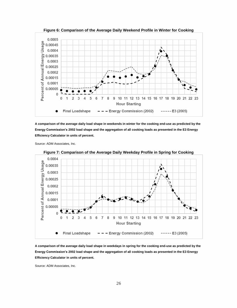
26
Figure 6: Comparison of the Average Daily Weekend Profile in Winter for Cooking
A comparison of the average daily load shape in weekends in winter for the cooking end-use as predicted by the
Energy Commission’s 2002 load shape and the aggregation of all cooking loads as presented in the E3 Energy
Efficiency Calculator in units of percent.
Source: ADM Associates, Inc.
Figure 7: Comparison of the Average Daily Weekday Profile in Spring for Cooking
A comparison of the average daily load shape in weekdays in spring for the cooking end-use as predicted by the
Energy Commission’s 2002 load shape and the aggregation of all cooking loads as presented in the E3 Energy
Efficiency Calculator in units of percent.
Source: ADM Associates, Inc.
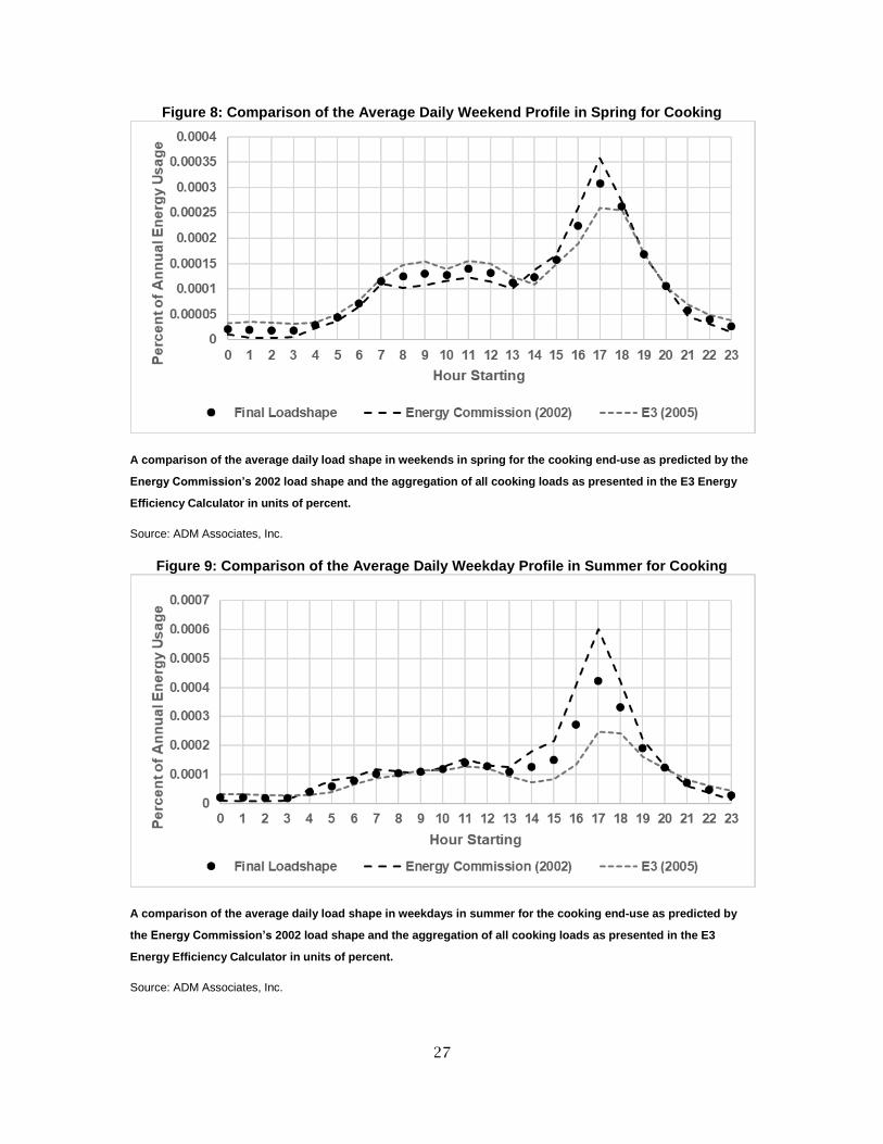
27
Figure 8: Comparison of the Average Daily Weekend Profile in Spring for Cooking
A comparison of the average daily load shape in weekends in spring for the cooking end-use as predicted by the
Energy Commission’s 2002 load shape and the aggregation of all cooking loads as presented in the E3 Energy
Efficiency Calculator in units of percent.
Source: ADM Associates, Inc.
Figure 9: Comparison of the Average Daily Weekday Profile in Summer for Cooking
A comparison of the average daily load shape in weekdays in summer for the cooking end-use as predicted by
the Energy Commission’s 2002 load shape and the aggregation of all cooking loads as presented in the E3
Energy Efficiency Calculator in units of percent.
Source: ADM Associates, Inc.
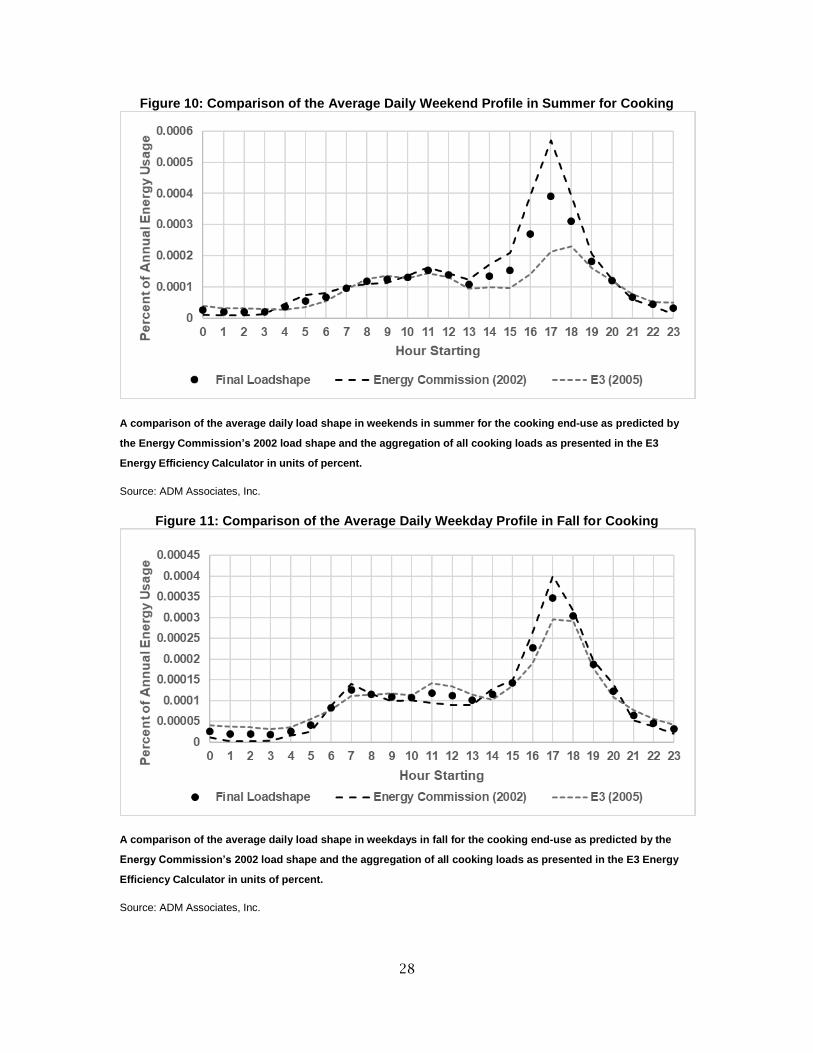
28
Figure 10: Comparison of the Average Daily Weekend Profile in Summer for Cooking
A comparison of the average daily load shape in weekends in summer for the cooking end-use as predicted by
the Energy Commission’s 2002 load shape and the aggregation of all cooking loads as presented in the E3
Energy Efficiency Calculator in units of percent.
Source: ADM Associates, Inc.
Figure 11: Comparison of the Average Daily Weekday Profile in Fall for Cooking
A comparison of the average daily load shape in weekdays in fall for the cooking end-use as predicted by the
Energy Commission’s 2002 load shape and the aggregation of all cooking loads as presented in the E3 Energy
Efficiency Calculator in units of percent.
Source: ADM Associates, Inc.
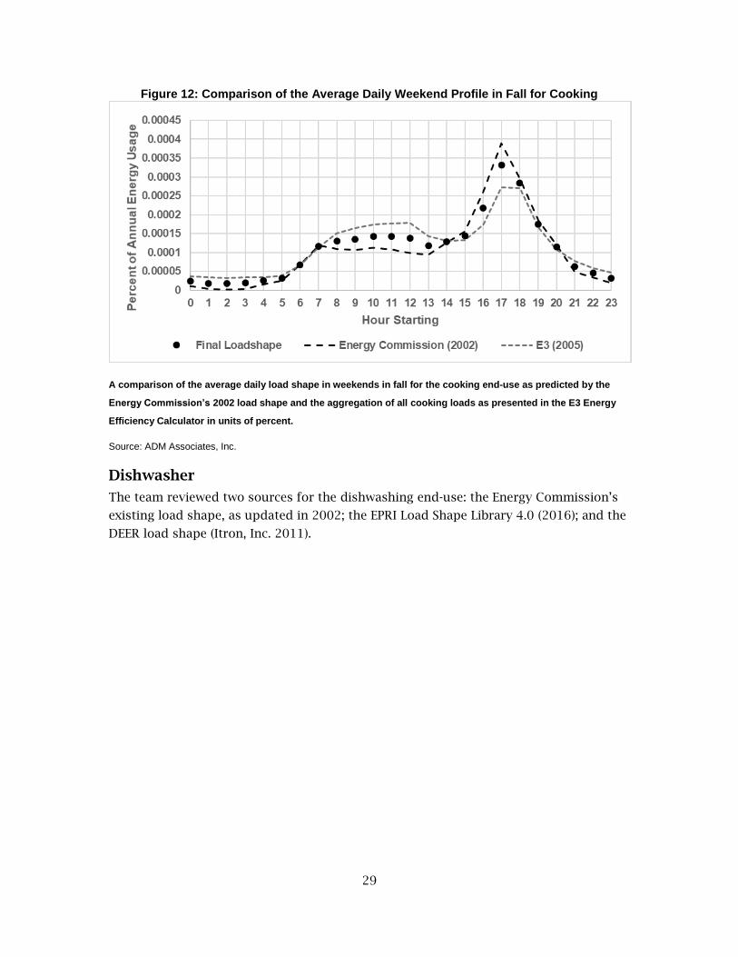
29
Figure 12: Comparison of the Average Daily Weekend Profile in Fall for Cooking
A comparison of the average daily load shape in weekends in fall for the cooking end-use as predicted by the
Energy Commission’s 2002 load shape and the aggregation of all cooking loads as presented in the E3 Energy
Efficiency Calculator in units of percent.
Source: ADM Associates, Inc.
Dishwasher
The team reviewed two sources for the dishwashing end-use: the Energy Commission’s
existing load shape, as updated in 2002; the EPRI Load Shape Library 4.0 (2016); and the
DEER load shape (Itron, Inc. 2011).

30
Figure 13 through

31
Figure 21 present the monthly energy usage and seasonal weekday/weekend daily
profiles for both sources and the aggregated load shape. In general, the average daily
load shapes appeared consistent with one another regardless of the season. Although
the monthly energy usage differed from one another, an argument could not be made as
to why one profile may be more valid than the other, therefore, ADM averaged all
profiles together to create the final load shape.
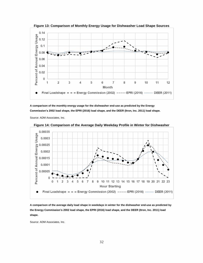
32
Figure 13: Comparison of Monthly Energy Usage for Dishwasher Load Shape Sources
A comparison of the monthly energy usage for the dishwasher end-use as predicted by the Energy
Commission’s 2002 load shape, the EPRI (2016) load shape, and the DEER (Itron, Inc. 2011) load shape.
Source: ADM Associates, Inc.
Figure 14: Comparison of the Average Daily Weekday Profile in Winter for Dishwasher
A comparison of the average daily load shape in weekdays in winter for the dishwasher end-use as predicted by
the Energy Commission’s 2002 load shape, the EPRI (2016) load shape, and the DEER (Itron, Inc. 2011) load
shape.
Source: ADM Associates, Inc.
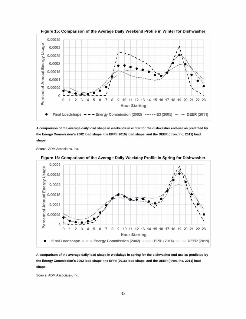
33
Figure 15: Comparison of the Average Daily Weekend Profile in Winter for Dishwasher
A comparison of the average daily load shape in weekends in winter for the dishwasher end-use as predicted by
the Energy Commission’s 2002 load shape, the EPRI (2016) load shape, and the DEER (Itron, Inc. 2011) load
shape.
Source: ADM Associates, Inc.
Figure 16: Comparison of the Average Daily Weekday Profile in Spring for Dishwasher
A comparison of the average daily load shape in weekdays in spring for the dishwasher end-use as predicted by
the Energy Commission’s 2002 load shape, the EPRI (2016) load shape, and the DEER (Itron, Inc. 2011) load
shape.
Source: ADM Associates, Inc.

34
Figure 17: Comparison of the Average Daily Weekend Profile in Spring for Dishwasher
A comparison of the average daily load shape in weekends in spring for the dishwasher end-use as predicted by
the Energy Commission’s 2002 load shape, the EPRI (2016) load shape, and the DEER (Itron, Inc. 2011) load
shape.
Source: ADM Associates, Inc.
Figure 18: Comparison of the Average Daily Weekday Profile in Summer for Dishwasher
A comparison of the average daily load shape in weekdays in summer for the dishwasher end-use as predicted
by the Energy Commission’s 2002 load shape, the EPRI (2016) load shape, and the DEER (Itron, Inc. 2011) load
shape.
Source: ADM Associates, Inc.
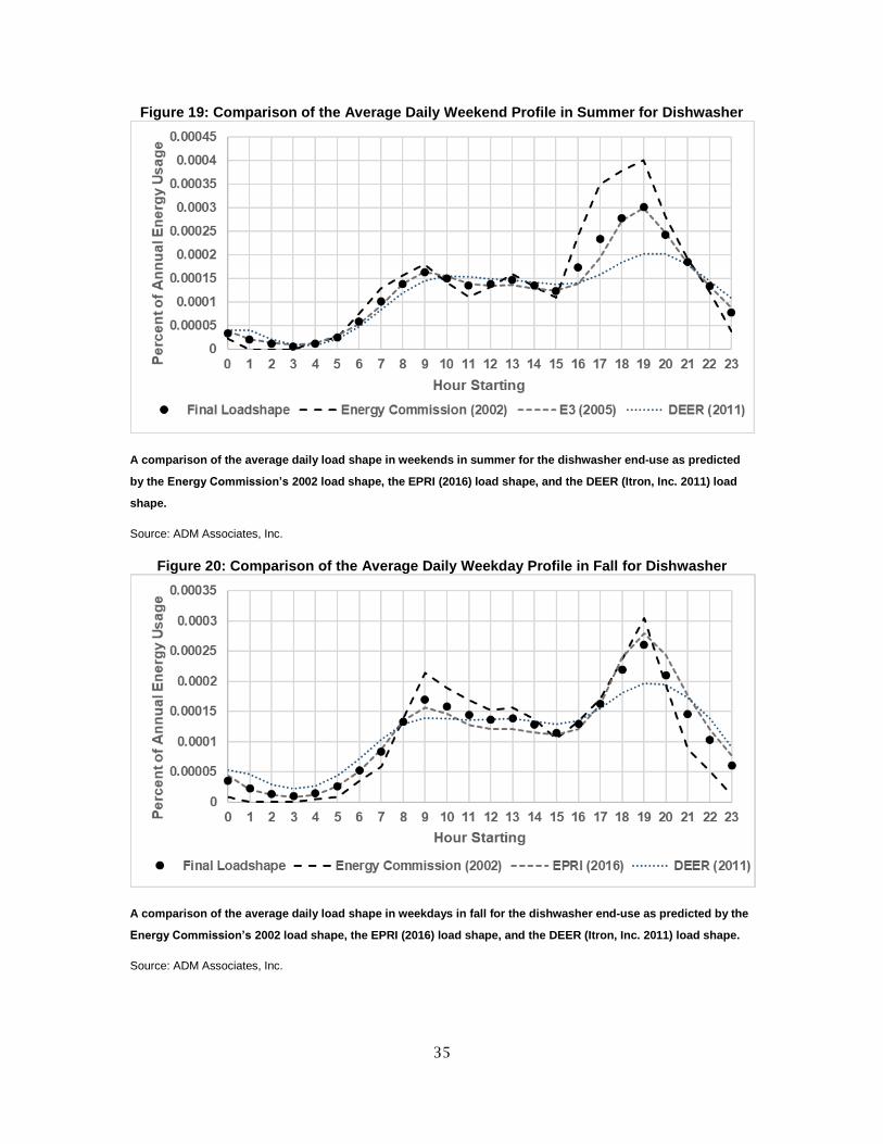
35
Figure 19: Comparison of the Average Daily Weekend Profile in Summer for Dishwasher
A comparison of the average daily load shape in weekends in summer for the dishwasher end-use as predicted
by the Energy Commission’s 2002 load shape, the EPRI (2016) load shape, and the DEER (Itron, Inc. 2011) load
shape.
Source: ADM Associates, Inc.
Figure 20: Comparison of the Average Daily Weekday Profile in Fall for Dishwasher
A comparison of the average daily load shape in weekdays in fall for the dishwasher end-use as predicted by the
Energy Commission’s 2002 load shape, the EPRI (2016) load shape, and the DEER (Itron, Inc. 2011) load shape.
Source: ADM Associates, Inc.
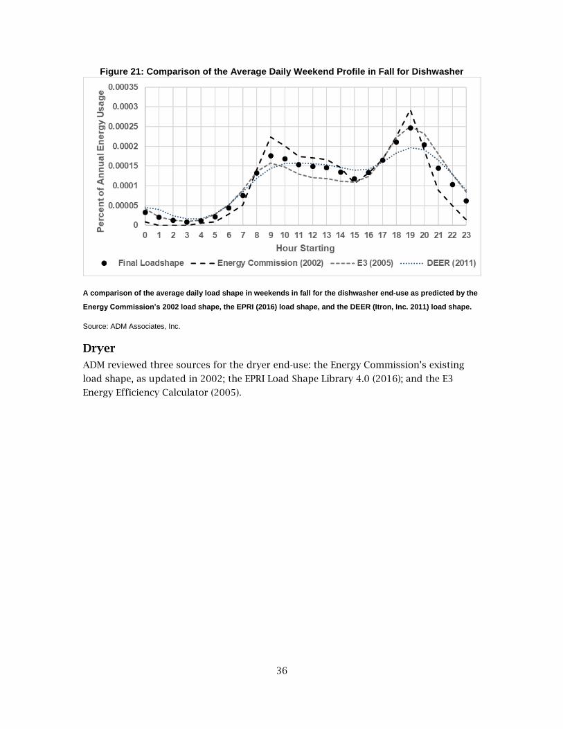
36
Figure 21: Comparison of the Average Daily Weekend Profile in Fall for Dishwasher
A comparison of the average daily load shape in weekends in fall for the dishwasher end-use as predicted by the
Energy Commission’s 2002 load shape, the EPRI (2016) load shape, and the DEER (Itron, Inc. 2011) load shape.
Source: ADM Associates, Inc.
Dryer
ADM reviewed three sources for the dryer end-use: the Energy Commission’s existing
load shape, as updated in 2002; the EPRI Load Shape Library 4.0 (2016); and the E3
Energy Efficiency Calculator (2005).

37
Figure 22 through

38
Figure 30 present the monthly energy use and seasonal weekday/weekend daily profiles
for sources and the aggregated load shape. In general, the average daily load shapes
appeared consistent with one another regardless of the season. Although the monthly
energy use differed from one another, an argument could not be made as to why one
profile may be more valid than the other, therefore, ADM averaged all profiles together
to create the final load shape.
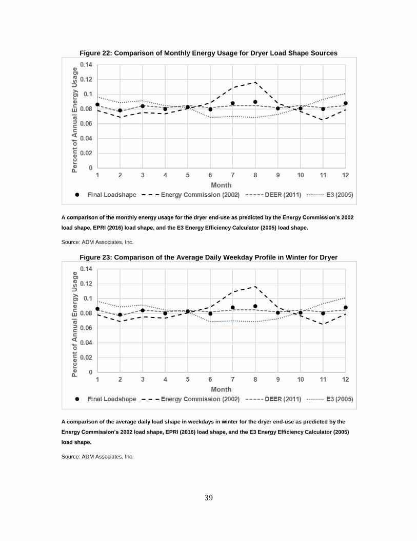
39
Figure 22: Comparison of Monthly Energy Usage for Dryer Load Shape Sources
A comparison of the monthly energy usage for the dryer end-use as predicted by the Energy Commission’s 2002
load shape, EPRI (2016) load shape, and the E3 Energy Efficiency Calculator (2005) load shape.
Source: ADM Associates, Inc.
Figure 23: Comparison of the Average Daily Weekday Profile in Winter for Dryer
A comparison of the average daily load shape in weekdays in winter for the dryer end-use as predicted by the
Energy Commission’s 2002 load shape, EPRI (2016) load shape, and the E3 Energy Efficiency Calculator (2005)
load shape.
Source: ADM Associates, Inc.
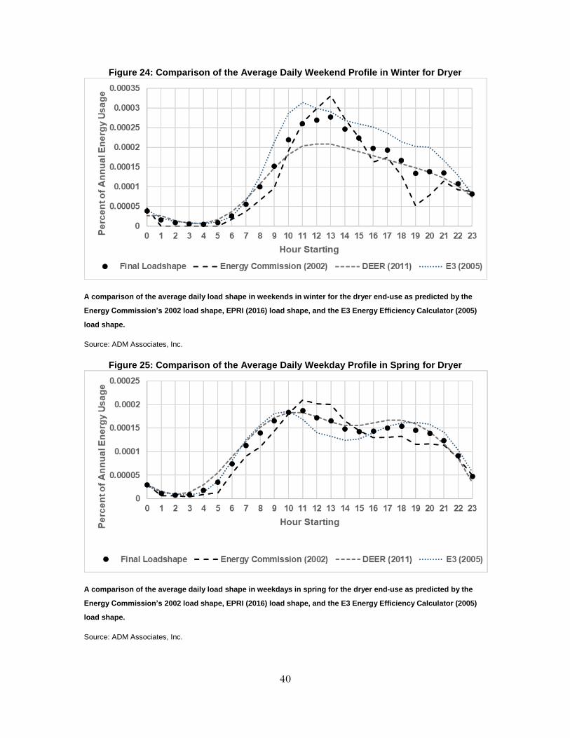
40
Figure 24: Comparison of the Average Daily Weekend Profile in Winter for Dryer
A comparison of the average daily load shape in weekends in winter for the dryer end-use as predicted by the
Energy Commission’s 2002 load shape, EPRI (2016) load shape, and the E3 Energy Efficiency Calculator (2005)
load shape.
Source: ADM Associates, Inc.
Figure 25: Comparison of the Average Daily Weekday Profile in Spring for Dryer
A comparison of the average daily load shape in weekdays in spring for the dryer end-use as predicted by the
Energy Commission’s 2002 load shape, EPRI (2016) load shape, and the E3 Energy Efficiency Calculator (2005)
load shape.
Source: ADM Associates, Inc.

41
Figure 26: Comparison of the Average Daily Weekend Profile in Spring for Dryer
A comparison of the average daily load shape in weekends in spring for the dryer end-use as predicted by the
Energy Commission’s 2002 load shape, EPRI (2016) load shape, and the E3 Energy Efficiency Calculator (2005)
load shape.
Source: ADM Associates, Inc.
Figure 27: Comparison of the Average Daily Weekday Profile in Summer for Dryer
A comparison of the average daily load shape in weekdays in summer for the dryer end-use as predicted by the
Energy Commission’s 2002 load shape, EPRI (2016) load shape, and the E3 Energy Efficiency Calculator (2005)
load shape.
Source: ADM Associates, Inc.
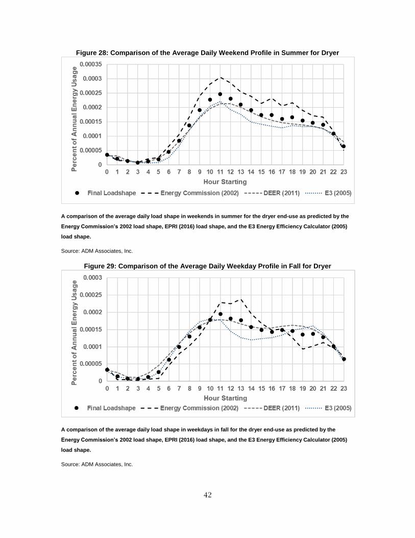
42
Figure 28: Comparison of the Average Daily Weekend Profile in Summer for Dryer
A comparison of the average daily load shape in weekends in summer for the dryer end-use as predicted by the
Energy Commission’s 2002 load shape, EPRI (2016) load shape, and the E3 Energy Efficiency Calculator (2005)
load shape.
Source: ADM Associates, Inc.
Figure 29: Comparison of the Average Daily Weekday Profile in Fall for Dryer
A comparison of the average daily load shape in weekdays in fall for the dryer end-use as predicted by the
Energy Commission’s 2002 load shape, EPRI (2016) load shape, and the E3 Energy Efficiency Calculator (2005)
load shape.
Source: ADM Associates, Inc.

43
Figure 30: Comparison of the Average Daily Weekend Profile in Fall for Dryer
A comparison of the average daily load shape in weekends in fall for the dryer end-use as predicted by the
Energy Commission’s 2002 load shape, EPRI (2016) load shape, and the E3 Energy Efficiency Calculator (2005)
load shape.
Source: ADM Associates, Inc.
Freezer
ADM reviewed two sources for the freezer end-use: the DEER (2011) and the E3 Energy
Efficiency Calculator (2005).

44
Figure 31 through

45
Figure 39 present the monthly energy usage and seasonal weekday/weekend daily
profiles for both sources and the aggregated load shape. In general, there was good
correlation, r=0.82, between both sources, therefore, ADM averaged all profiles together
to create the final load shape.
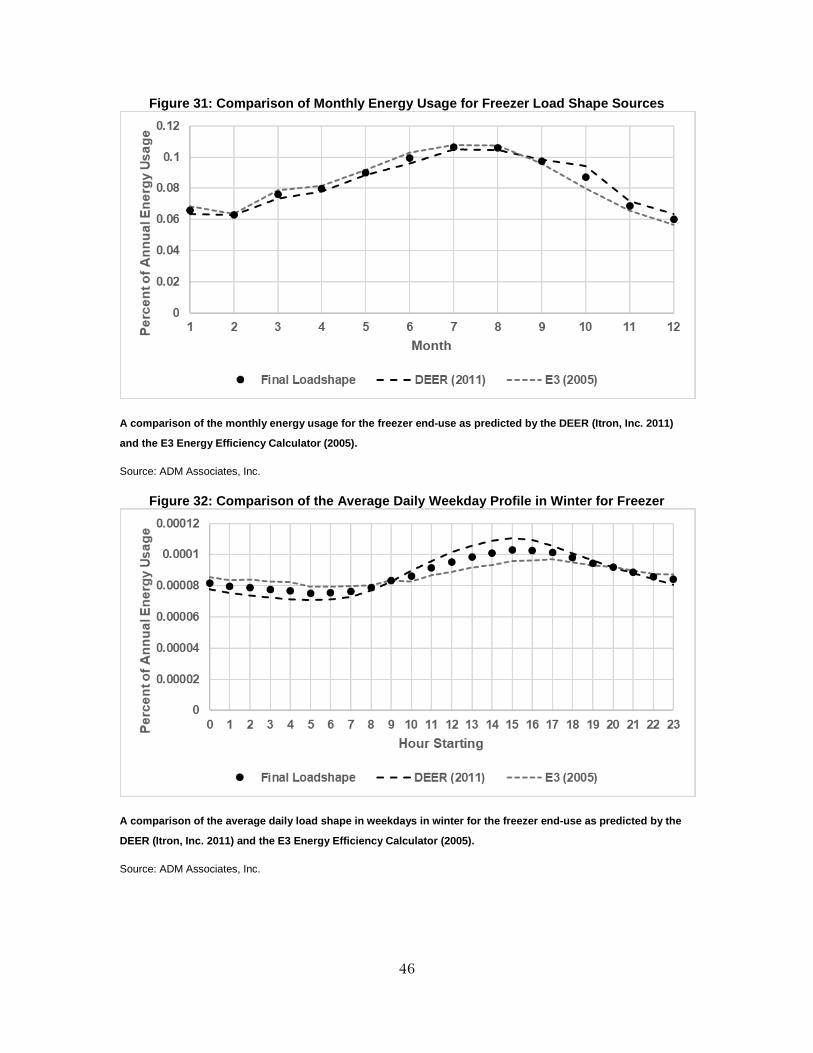
46
Figure 31: Comparison of Monthly Energy Usage for Freezer Load Shape Sources
A comparison of the monthly energy usage for the freezer end-use as predicted by the DEER (Itron, Inc. 2011)
and the E3 Energy Efficiency Calculator (2005).
Source: ADM Associates, Inc.
Figure 32: Comparison of the Average Daily Weekday Profile in Winter for Freezer
A comparison of the average daily load shape in weekdays in winter for the freezer end-use as predicted by the
DEER (Itron, Inc. 2011) and the E3 Energy Efficiency Calculator (2005).
Source: ADM Associates, Inc.
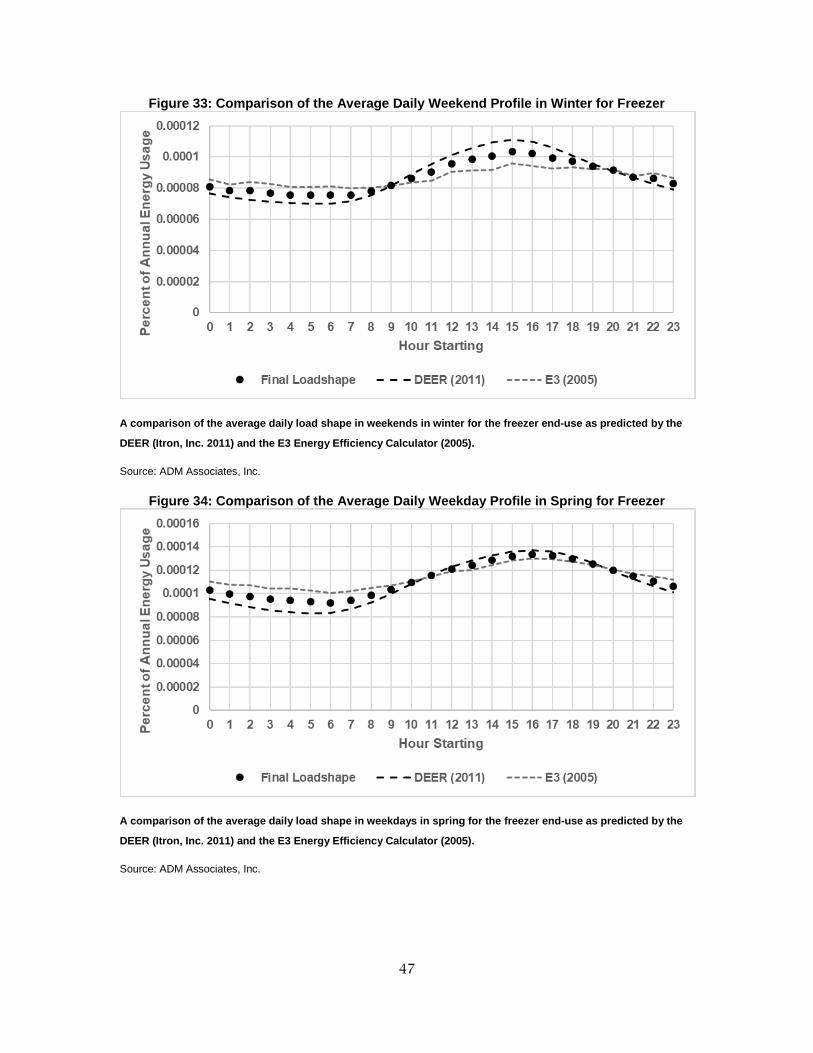
47
Figure 33: Comparison of the Average Daily Weekend Profile in Winter for Freezer
A comparison of the average daily load shape in weekends in winter for the freezer end-use as predicted by the
DEER (Itron, Inc. 2011) and the E3 Energy Efficiency Calculator (2005).
Source: ADM Associates, Inc.
Figure 34: Comparison of the Average Daily Weekday Profile in Spring for Freezer
A comparison of the average daily load shape in weekdays in spring for the freezer end-use as predicted by the
DEER (Itron, Inc. 2011) and the E3 Energy Efficiency Calculator (2005).
Source: ADM Associates, Inc.

48
Figure 35: Comparison of the Average Daily Weekend Profile in Spring for Freezer
A comparison of the average daily load shape in weekends in spring for the freezer end-use as predicted by the
DEER (Itron, Inc. 2011) and the E3 Energy Efficiency Calculator (2005).
Source: ADM Associates, Inc.
Figure 36: Comparison of the Average Daily Weekday Profile in Summer for Freezer
A comparison of the average daily load shape in weekdays in summer for the freezer end-use as predicted by the
DEER (Itron, Inc. 2011) and the E3 Energy Efficiency Calculator (2005).
Source: ADM Associates, Inc.

49
Figure 37: Comparison of the Average Daily Weekend Profile in Summer for Freezer
A comparison of the average daily load shape in weekends in summer for the freezer end-use as predicted by the
DEER (Itron, Inc. 2011) and the E3 Energy Efficiency Calculator (2005).
Source: ADM Associates, Inc.
Figure 38: Comparison of the Average Daily Weekday Profile in Fall for Freezer
A comparison of the average daily load shape in weekdays in fall for the Freezer end-use as predicted by the
DEER (Itron, Inc. 2011) and the E3 Energy Efficiency Calculator (2005).
Source: ADM Associates, Inc.

50
Figure 39: Comparison of the Average Daily Weekend Profile in Fall for Freezer
A comparison of the average daily load shape in weekends in fall for the Freezer end-use as predicted by the
DEER (Itron, Inc. 2011) and the E3 Energy Efficiency Calculator (2005).
Source: ADM Associates, Inc.
Lighting
ADM reviewed three sources for the lighting end-use: a 2016 lighting study from the
Northwest (Grist 2016), and two ADM work papers—one for a client in Nevada in one for
a client in Pennsylvania.

51
Figure 40 through

52
Figure 48 present the monthly energy usage and seasonal weekday/weekend daily
profiles for both sources and the aggregated load shape. In general, there was good
correspondence between all sources, r > 0.87 for all shapes. Therefore, ADM averaged all
profiles together to create the final load shape.

53
Figure 40: Comparison of Monthly Energy Usage for Lighting Load Shape Sources
A comparison of the monthly energy usage for the lighting end-use as predicted by the 2016 Grist study and the
two ADM work papers.
Source: ADM Associates, Inc.
Figure 41: Comparison of the Average Daily Weekday Profile in Winter for Lighting
A comparison of the average daily load shape in weekdays in winter for the lighting end-use as predicted by the
2016 Grist study and the two ADM work papers.
Source: ADM Associates, Inc.
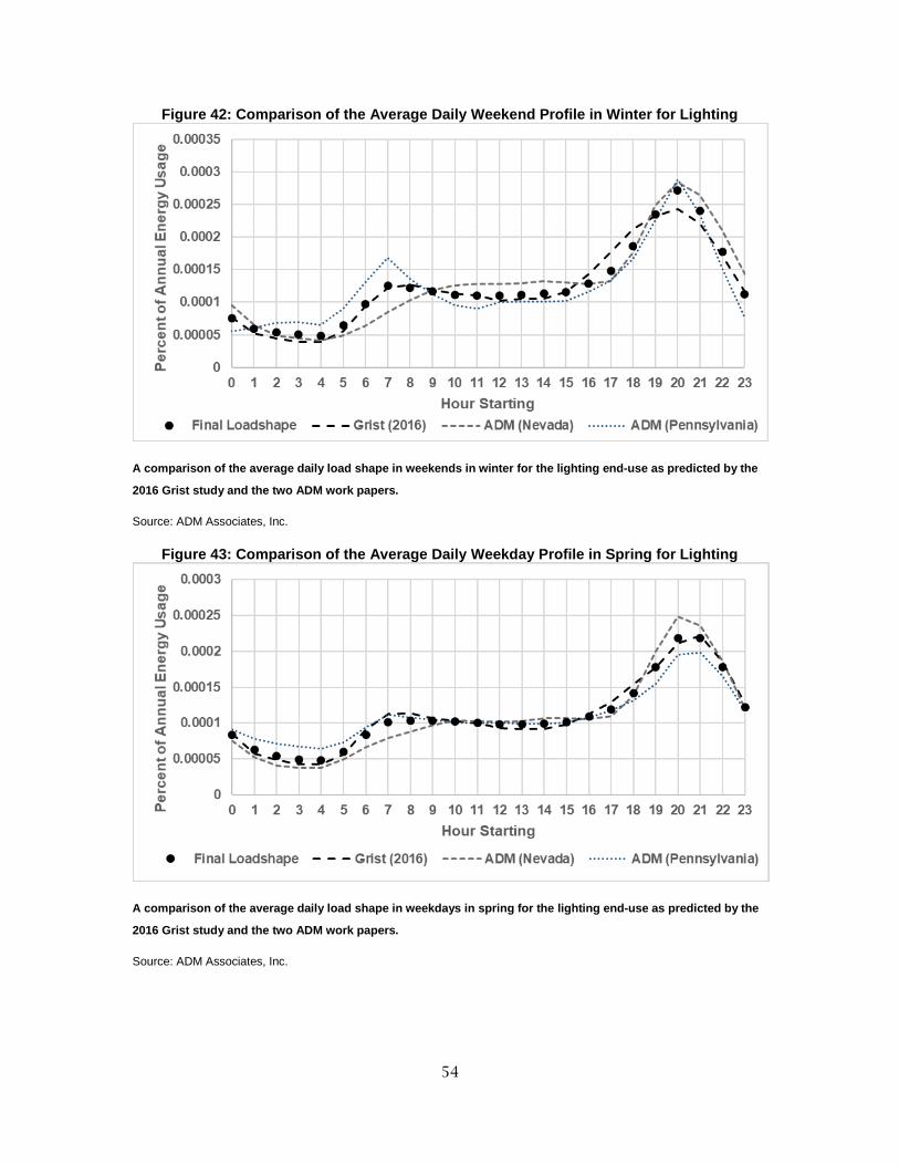
54
Figure 42: Comparison of the Average Daily Weekend Profile in Winter for Lighting
A comparison of the average daily load shape in weekends in winter for the lighting end-use as predicted by the
2016 Grist study and the two ADM work papers.
Source: ADM Associates, Inc.
Figure 43: Comparison of the Average Daily Weekday Profile in Spring for Lighting
A comparison of the average daily load shape in weekdays in spring for the lighting end-use as predicted by the
2016 Grist study and the two ADM work papers.
Source: ADM Associates, Inc.

55
Figure 44: Comparison of the Average Daily Weekend Profile in Spring for Lighting
A comparison of the average daily load shape in weekends in spring for the lighting end-use as predicted by the
2016 Grist study and the two ADM work papers.
Source: ADM Associates, Inc.
Figure 45: Comparison of the Average Daily Weekday Profile in Summer for Lighting
A comparison of the average daily load shape in weekdays in summer for the lighting end-use as predicted by
the 2016 Grist study and the two ADM work papers.
Source: ADM Associates, Inc.

56
Figure 46: Comparison of the Average Daily Weekend Profile in Summer for Lighting
A comparison of the average daily load shape in weekends in summer for the lighting end-use as predicted by
the 2016 Grist study and the two ADM work papers.
Source: ADM Associates, Inc.
Figure 47: Comparison of the Average Daily Weekday Profile in Fall for Lighting
A comparison of the average daily load shape in weekdays in fall for the lighting end-use as predicted by the
2016 Grist study and the two ADM work papers.
Source: ADM Associates, Inc.

57
Figure 48: Comparison of the Average Daily Weekend Profile in Fall for Lighting
A comparison of the average daily load shape in weekends in fall for the lighting end-use as predicted by the
2016 Grist study and the two ADM work papers.
Source: ADM Associates, Inc.
Pool Heater
The amount of resources with an isolated pool heater load shape was limited. Therefore,
ADM passed through the Energy Commission’s existing load shape as updated in 2002.

58
Figure 49 through

59
Figure 57 present the monthly energy use and seasonal weekday/weekend daily profiles
for this load shape.
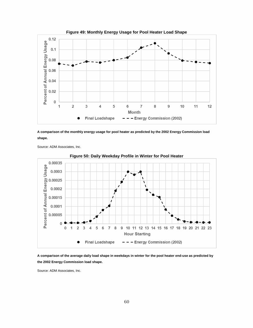
60
Figure 49: Monthly Energy Usage for Pool Heater Load Shape
A comparison of the monthly energy usage for pool heater as predicted by the 2002 Energy Commission load
shape.
Source: ADM Associates, Inc.
Figure 50: Daily Weekday Profile in Winter for Pool Heater
A comparison of the average daily load shape in weekdays in winter for the pool heater end-use as predicted by
the 2002 Energy Commission load shape.
Source: ADM Associates, Inc.
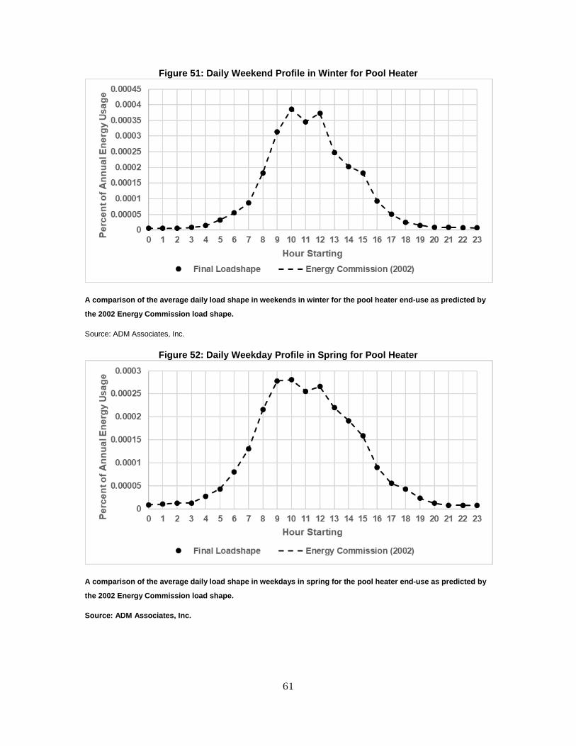
61
Figure 51: Daily Weekend Profile in Winter for Pool Heater
A comparison of the average daily load shape in weekends in winter for the pool heater end-use as predicted by
the 2002 Energy Commission load shape.
Source: ADM Associates, Inc.
Figure 52: Daily Weekday Profile in Spring for Pool Heater
A comparison of the average daily load shape in weekdays in spring for the pool heater end-use as predicted by
the 2002 Energy Commission load shape.
Source: ADM Associates, Inc.

62
Figure 53: Daily Weekend Profile in Spring for Pool Heater
A comparison of the average daily load shape in weekends in spring for the pool heater end-use as predicted by
the 2002 Energy Commission load shape.
Source: ADM Associates, Inc.
Figure 54: Daily Weekday Profile in Summer for Pool Heater
A comparison of the average daily load shape in weekdays in summer for the pool heater end-use as predicted
by the 2002 Energy Commission load shape.
Source: ADM Associates, Inc.

63
Figure 55: Daily Weekend Profile in Summer for Pool Heater
A comparison of the average daily load shape in weekends in summer for the pool heater end-use as predicted
by the 2002 Energy Commission load shape.
Source: ADM Associates, Inc.
Figure 56: Daily Weekday Profile in Fall for Pool Heater
A comparison of the average daily load shape in weekdays in fall for the pool heater end-use as predicted by the
2002 Energy Commission load shape.
Source: ADM Associates, Inc.

64
Figure 57: Daily Weekend Profile in Fall for Pool Heater
A comparison of the average daily load shape in weekends in fall for the pool heater end-use as predicted by the
2002 Energy Commission load shape.
Source: ADM Associates, Inc.
Pool Pump
ADM reviewed two sources for the pool pump end-use: the E3 Energy Efficiency
Calculator (2005) and a 2016 ADM study conducted for SMUD, which includes load
shapes for VSD pool pumps and non-VSD pool pumps.

65
Figure 58 through

66
Figure 66 present these load shapes. Although there was a fair amount of volatility
between the two data sources, an argument could not be made as to why one profile
may be more valid than the other, therefore, ADM averaged all profiles together to
create the final load shape.

67
Figure 58: Comparison of Monthly Energy Usage for Pool Pump Load Shape Sources
A comparison of the monthly energy usage for the pool pump end-use as predicted by the 2005 E3 Energy
Efficiency Calculator and the 2016 ADM study.
Source: ADM Associates, Inc.
Figure 59: Comparison of the Average Daily Weekday Profile in Winter for Pool Pump
A comparison of the average daily load shape in weekdays in winter for the pool pump end-use as predicted by
the 2005 E3 Energy Efficiency Calculator and the 2016 ADM study.
Source: ADM Associates, Inc.
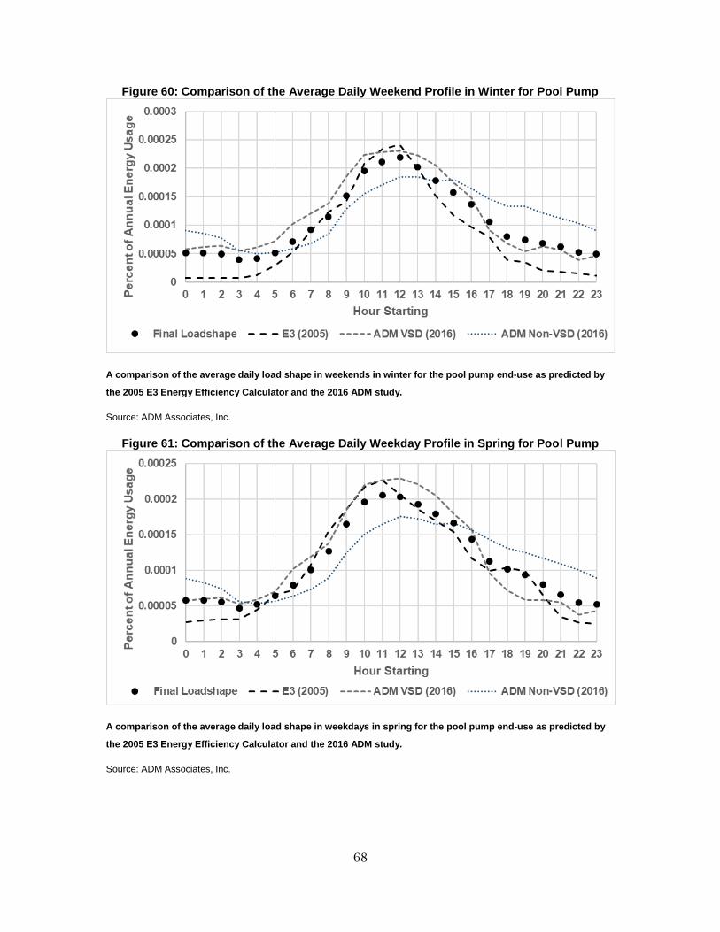
68
Figure 60: Comparison of the Average Daily Weekend Profile in Winter for Pool Pump
A comparison of the average daily load shape in weekends in winter for the pool pump end-use as predicted by
the 2005 E3 Energy Efficiency Calculator and the 2016 ADM study.
Source: ADM Associates, Inc.
Figure 61: Comparison of the Average Daily Weekday Profile in Spring for Pool Pump
A comparison of the average daily load shape in weekdays in spring for the pool pump end-use as predicted by
the 2005 E3 Energy Efficiency Calculator and the 2016 ADM study.
Source: ADM Associates, Inc.

69
Figure 62: Comparison of the Average Daily Weekend Profile in Spring for Pool Pump
A comparison of the average daily load shape in weekends in spring for the pool pump end-use as predicted by
the 2005 E3 Energy Efficiency Calculator and the 2016 ADM study.
Source: ADM Associates, Inc.
Figure 63: Comparison of the Average Daily Weekday Profile in Summer for Pool Pump
A comparison of the average daily load shape in weekdays in summer for the pool pump end-use as predicted by
the 2005 E3 Energy Efficiency Calculator and the 2016 ADM study.
Source: ADM Associates, Inc.
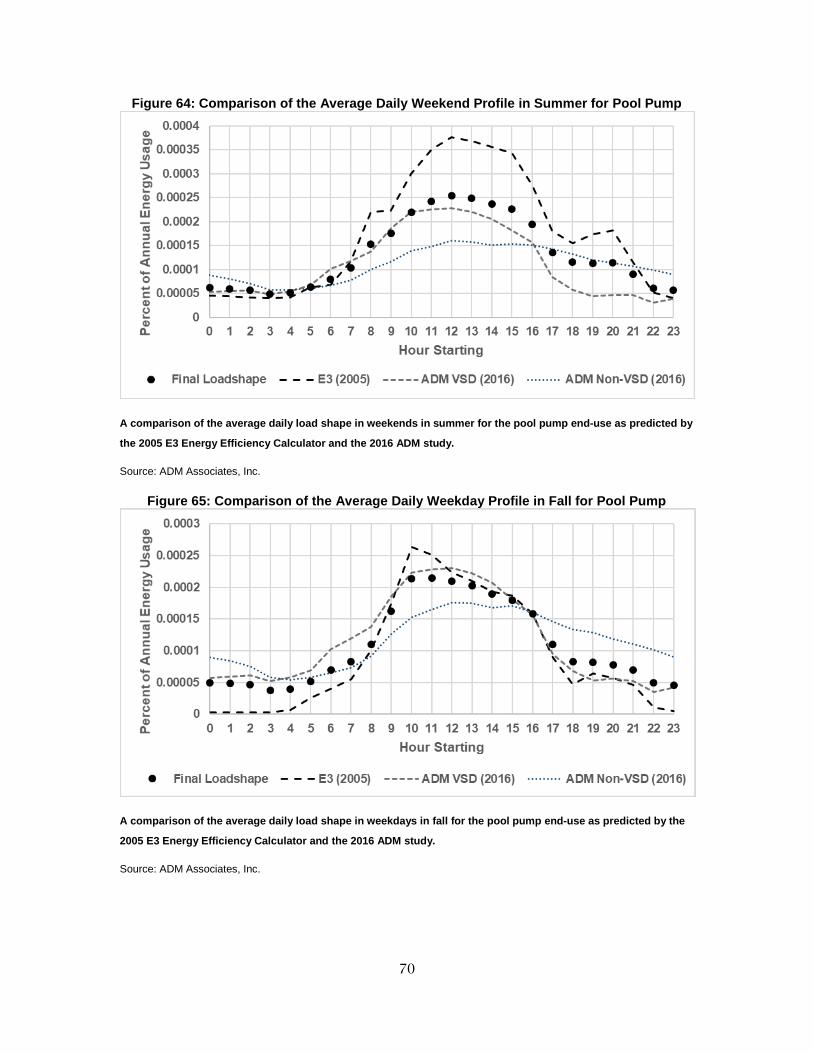
70
Figure 64: Comparison of the Average Daily Weekend Profile in Summer for Pool Pump
A comparison of the average daily load shape in weekends in summer for the pool pump end-use as predicted by
the 2005 E3 Energy Efficiency Calculator and the 2016 ADM study.
Source: ADM Associates, Inc.
Figure 65: Comparison of the Average Daily Weekday Profile in Fall for Pool Pump
A comparison of the average daily load shape in weekdays in fall for the pool pump end-use as predicted by the
2005 E3 Energy Efficiency Calculator and the 2016 ADM study.
Source: ADM Associates, Inc.
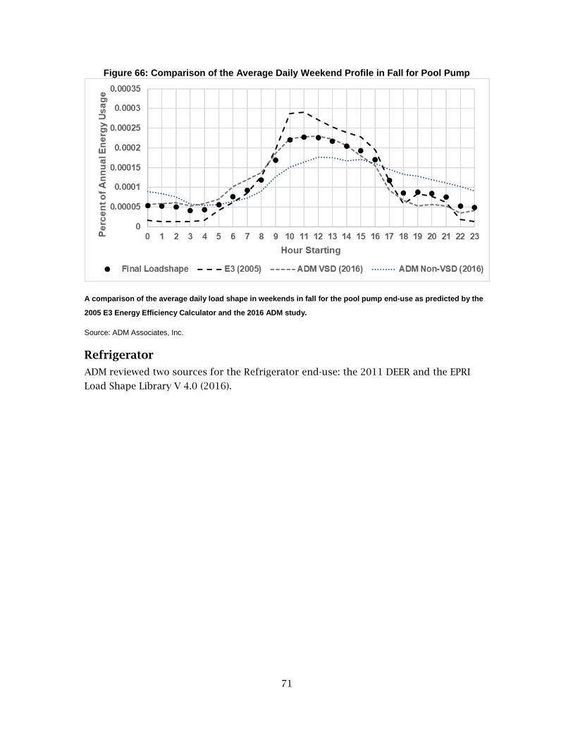
71
Figure 66: Comparison of the Average Daily Weekend Profile in Fall for Pool Pump
A comparison of the average daily load shape in weekends in fall for the pool pump end-use as predicted by the
2005 E3 Energy Efficiency Calculator and the 2016 ADM study.
Source: ADM Associates, Inc.
Refrigerator
ADM reviewed two sources for the Refrigerator end-use: the 2011 DEER and the EPRI
Load Shape Library V 4.0 (2016).

72
Figure 67 through

73
Figure 75 present the monthly energy usage and seasonal weekday/weekend daily
profiles for both sources and the aggregated load shape. In general, there was good
correspondence, r=0.82, between both sources, therefore, ADM averaged all profiles
together to create the final load shape.

74
Figure 67: Comparison of Monthly Energy Usage for Refrigerator Load Shape Sources
A comparison of the monthly energy usage for the refrigerator end-use as predicted by the DEER (Itron, Inc.
2011) and E3 Energy Efficiency Calculator (2005).
Source: ADM Associates, Inc.
Figure 68: Comparison of the Average Daily Weekday Profile in Winter for Refrigerator
A comparison of the average daily load shape in weekdays in winter for the refrigerator end-use as predicted by
the DEER (Itron, Inc. 2011) and E3 Energy Efficiency Calculator (2005).
Source: ADM Associates, Inc.
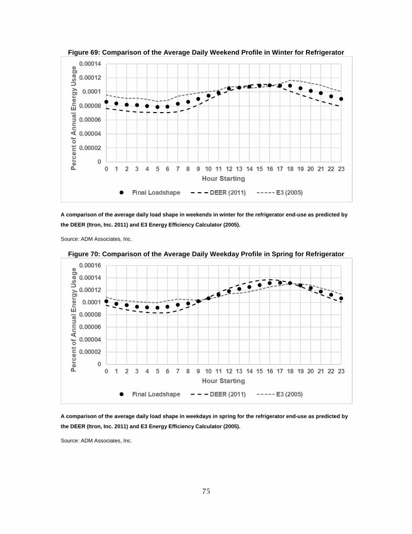
75
Figure 69: Comparison of the Average Daily Weekend Profile in Winter for Refrigerator
A comparison of the average daily load shape in weekends in winter for the refrigerator end-use as predicted by
the DEER (Itron, Inc. 2011) and E3 Energy Efficiency Calculator (2005).
Source: ADM Associates, Inc.
Figure 70: Comparison of the Average Daily Weekday Profile in Spring for Refrigerator
A comparison of the average daily load shape in weekdays in spring for the refrigerator end-use as predicted by
the DEER (Itron, Inc. 2011) and E3 Energy Efficiency Calculator (2005).
Source: ADM Associates, Inc.

76
Figure 71: Comparison of the Average Daily Weekend Profile in Spring for Refrigerator
A comparison of the average daily load shape in weekends in spring for the refrigerator end-use as predicted by
the DEER (Itron, Inc. 2011) and E3 Energy Efficiency Calculator (2005).
Source: ADM Associates, Inc.
Figure 72: Comparison of the Average Daily Weekday Profile in Summer for Refrigerator
A comparison of the average daily load shape in weekdays in summer for the refrigerator end-use as predicted
by the DEER (Itron, Inc. 2011) and E3 Energy Efficiency Calculator (2005). Source: ADM Associates, Inc.

77
Figure 73: Comparison of the Average Daily Weekend Profile in Summer for Refrigerator
A comparison of the average daily load shape in weekends in summer for the refrigerator end-use as predicted
by the DEER (Itron, Inc. 2011) and E3 Energy Efficiency Calculator (2005).
Source: ADM Associates, Inc.
Figure 74: Comparison of the Average Daily Weekday Profile in Fall for Refrigerator
A comparison of the average daily load shape in weekdays in fall for the refrigerator end-use as predicted by the
DEER (Itron, Inc. 2011) and E3 Energy Efficiency Calculator (2005).
Source: ADM Associates, Inc.
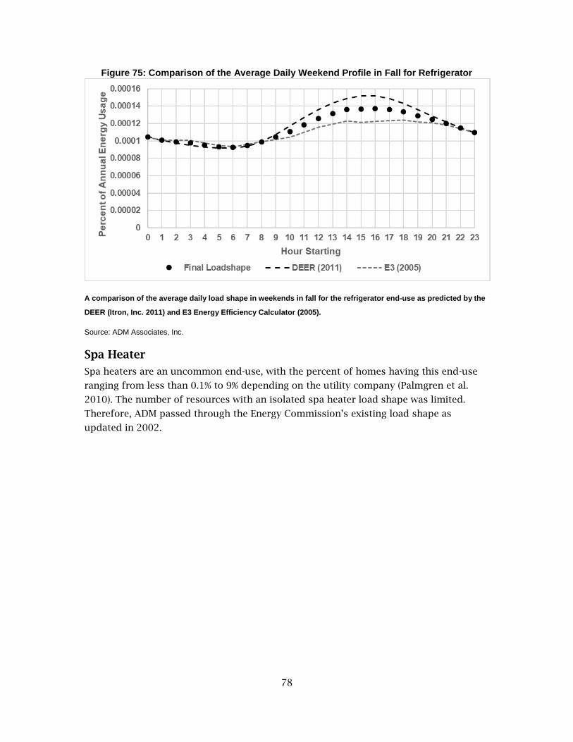
78
Figure 75: Comparison of the Average Daily Weekend Profile in Fall for Refrigerator
A comparison of the average daily load shape in weekends in fall for the refrigerator end-use as predicted by the
DEER (Itron, Inc. 2011) and E3 Energy Efficiency Calculator (2005).
Source: ADM Associates, Inc.
Spa Heater
Spa heaters are an uncommon end-use, with the percent of homes having this end-use
ranging from less than 0.1% to 9% depending on the utility company (Palmgren et al.
2010). The number of resources with an isolated spa heater load shape was limited.
Therefore, ADM passed through the Energy Commission’s existing load shape as
updated in 2002.

79
Figure 76 through

80
Figure 84 present the monthly energy usage and seasonal weekday/weekend daily
profiles for this load shape.

81
Figure 76: Monthly Energy Usage for Spa Heater Load Shape
A comparison of the monthly energy usage for spa heater as predicted by the 2002 Energy Commission load
shape.
Source: ADM Associates, Inc.
Figure 77: Daily Weekday Profile in Winter for Spa Heater
A comparison of the average daily load shape in weekdays in winter for the spa heater end-use as predicted by
the 2002 Energy Commission load shape.
Source: ADM Associates, Inc.

82
Figure 78: Daily Weekend Profile in Winter for Spa Heater
A comparison of the average daily load shape in weekends in winter for the spa heater end-use as predicted by
the 2002 Energy Commission load shape.
Source: ADM Associates, Inc.
Figure 79: Daily Weekday Profile in Spring for Spa Heater
A comparison of the average daily load shape in weekdays in spring for the spa heater end-use as predicted by
the 2002 Energy Commission load shape.
Source: ADM Associates, Inc.

83
Figure 80: Daily Weekend Profile in Spring for Spa Heater
A comparison of the average daily load shape in weekends in spring for the spa heater end-use as predicted by
the 2002 Energy Commission load shape.
Source: ADM Associates, Inc.
Figure 81: Daily Weekday Profile in Summer for Spa Heater
A comparison of the average daily load shape in weekdays in summer for the spa heater end-use as predicted by
the 2002 Energy Commission load shape.
Source: ADM Associates, Inc.

84
Figure 82: Daily Weekend Profile in Summer for Spa Heater
A comparison of the average daily load shape in weekends in summer for the spa heater end-use as predicted by
the 2002 Energy Commission load shape.
Source: ADM Associates, Inc.
Figure 83: Daily Weekday Profile in Fall for Spa Heater
A comparison of the average daily load shape in weekdays in fall for the spa heater end-use as predicted by the
2002 Energy Commission load shape.
Source: ADM Associates, Inc.

85
Figure 84: Daily Weekend Profile in Fall for Spa Heater
A comparison of the average daily load shape in weekends in fall for the spa heater end-use as predicted by the
2002 Energy Commission load shape.
Source: ADM Associates, Inc.
Spa Pump
Spa pumps are not a well-studied end-use. None of the sources reviewed as part of
ADM’s literature review featured an isolate spa pump load shape; instead choosing to
aggregate across spa and pool pumps. Part of this may be due to spa pumps
contributing less than 0.1% of the average annual energy load of a home, thereby
making its impact low compared to other end-uses (Palmgren et al. 2010). ADM
generally assumed that the load shape for spa pumps should be collinear to the load
shape for pool pumps, with a more distributed load shape as energy demand of a spa
pump is lower than that of a pool pump. To accomplish this, ADM used the
consolidated pool pump load shape and averaged it with a static flat load shape.

86
Figure 85 through

87
Figure 93 present the monthly energy usage and seasonal weekday/weekend daily
profiles for this load shape.

88
Figure 85: Monthly Energy Usage for Spa Pump Load Shape
A comparison of the monthly energy usage for spa pump as compared to the pool pump load shape and a static
flat load shape.
Source: ADM Associates, Inc.
Figure 86: Daily Weekday Profile in Winter for Spa Pump
A comparison of the average daily load shape in weekdays in winter for spa pump as compared to the pool pump
load shape and a static flat load shape.
Source: ADM Associates, Inc.

89
Figure 87: Daily Weekend Profile in Winter for Spa Pump
A comparison of the average daily load shape in weekends in winter for spa pump as compared to the pool pump
load shape and a static flat load shape.
Source: ADM Associates, Inc.
Figure 88: Daily Weekday Profile in Spring for Spa Pump
A comparison of the average daily load shape in weekdays in spring for spa pump as compared to the pool pump
load shape and a static flat load shape.
Source: ADM Associates, Inc.

90
Figure 89: Daily Weekend Profile in Spring for Spa Pump
A comparison of the average daily load shape in weekends in spring for spa pump as compared to the pool pump
load shape and a static flat load shape.
Source: ADM Associates, Inc.
Figure 90: Daily Weekday Profile in Summer for Spa Pump
A comparison of the average daily load shape in weekdays in summer for spa pump as compared to the pool
pump load shape and a static flat load shape.
Source: ADM Associates, Inc.

91
Figure 91: Daily Weekend Profile in Summer for Spa Pump
A comparison of the average daily load shape in weekends in summer for spa pump as compared to the pool
pump load shape and a static flat load shape.
Source: ADM Associates, Inc.
Figure 92: Daily Weekday Profile in Fall for Spa Pump
A comparison of the average daily load shape in weekdays in fall for spa pump as compared to the pool pump
load shape and a static flat load shape.
Source: ADM Associates, Inc.

92
Figure 93: Daily Weekend Profile in Fall for Spa Pump
A comparison of the average daily load shape in weekends in fall for spa pump as compared to the pool pump
load shape and a static flat load shape.
Source: ADM Associates, Inc.
Television
In addition to the Energy Commission’s 2002 load shape, ADM was able to locate one
additional data source for a television load shape. This secondary source came from the
2016 EPRI Load Shape Library 4.0. Unlike the Energy Commission load shape, however,
the EPRI shape also includes consumer electronics such as telecommunications,
computers, etc. In general, load shapes for television or consumer electronics should
follow a similar pattern to a lighting load shape, with an off-hours peak in the mid-
evening and a low-point in the early morning. Because the EPRI load shape showed
anomalous patterning, ADM reverted to using the Energy Commission’s 2002 load shape
for television.

93
Figure 94 through

94
Figure 102 present this comparison.

95
Figure 94: Comparison of Monthly Energy Usage for Television Load Shape
A comparison of the monthly energy usage for television between the 2002 Energy Commission load shape and
the 2016 EPRI load shape.
Source: ADM Associates, Inc.
Figure 95: Comparison of Daily Weekday Profile in Winter for Television
A comparison of the average daily load shape in weekdays in winter for television between the 2002 Energy
Commission load shape and the 2016 EPRI load shape.
Source: ADM Associates, Inc.
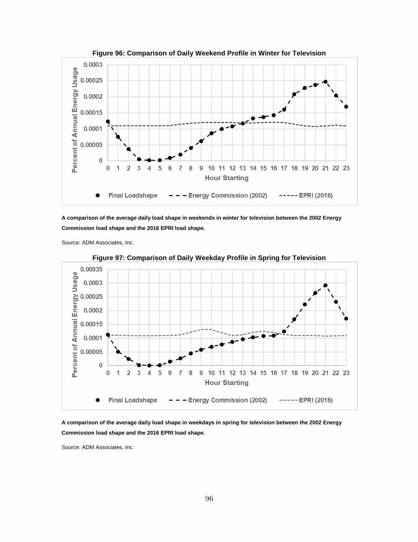
96
Figure 96: Comparison of Daily Weekend Profile in Winter for Television
A comparison of the average daily load shape in weekends in winter for television between the 2002 Energy
Commission load shape and the 2016 EPRI load shape.
Source: ADM Associates, Inc.
Figure 97: Comparison of Daily Weekday Profile in Spring for Television
A comparison of the average daily load shape in weekdays in spring for television between the 2002 Energy
Commission load shape and the 2016 EPRI load shape.
Source: ADM Associates, Inc.

97
Figure 98: Comparison of Daily Weekend Profile in Spring for Television
A comparison of the average daily load shape in weekends in spring for television between the 2002 Energy
Commission load shape and the 2016 EPRI load shape.
Source: ADM Associates, Inc.
Figure 99: Comparison of Daily Weekday Profile in Summer for Television
A comparison of the average daily load shape in weekdays in summer for television between the 2002 Energy
Commission load shape and the 2016 EPRI load shape.
Source: ADM Associates, Inc.
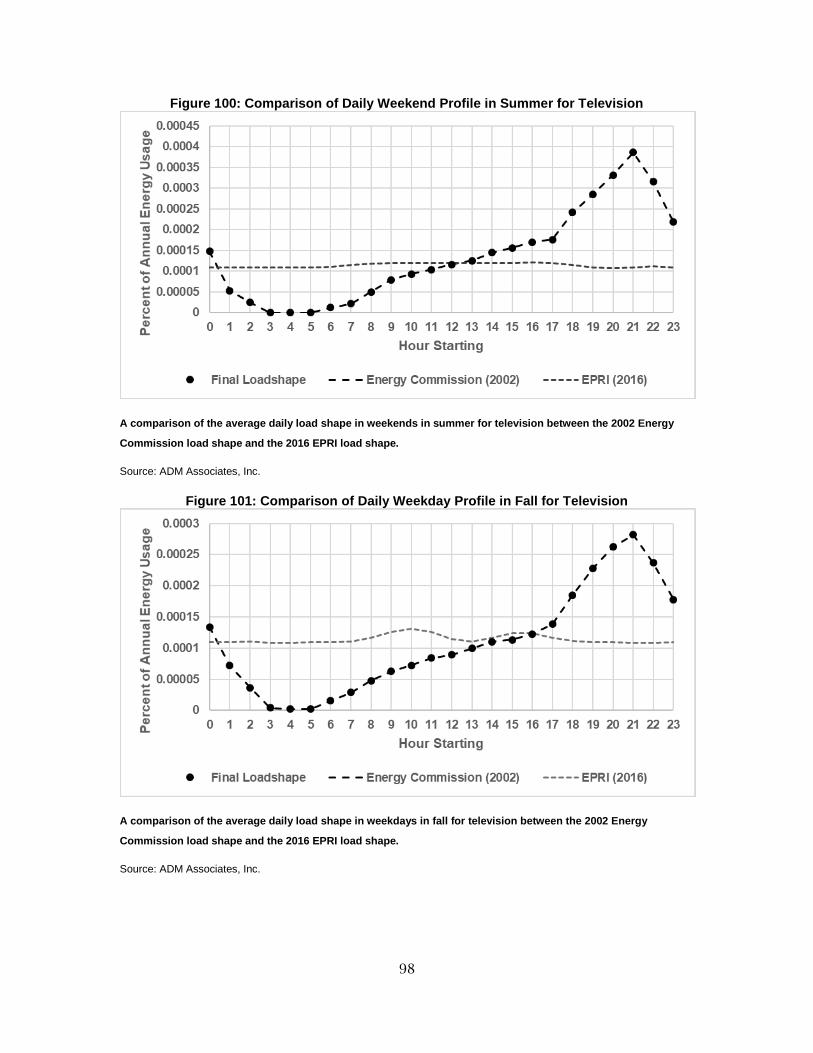
98
Figure 100: Comparison of Daily Weekend Profile in Summer for Television
A comparison of the average daily load shape in weekends in summer for television between the 2002 Energy
Commission load shape and the 2016 EPRI load shape.
Source: ADM Associates, Inc.
Figure 101: Comparison of Daily Weekday Profile in Fall for Television
A comparison of the average daily load shape in weekdays in fall for television between the 2002 Energy
Commission load shape and the 2016 EPRI load shape.
Source: ADM Associates, Inc.

99
Figure 102: Comparison of Daily Weekend Profile in Fall for Television
A comparison of the average daily load shape in weekends in fall for television between the 2002 Energy
Commission load shape and the 2016 EPRI load shape.
Source: ADM Associates, Inc.
Washer
ADM reviewed four sources for the washer end-use: the existing Energy Commission
load shape from 2002, the 2016 EPRI Load Shape Library 4.0, the DEER (Itron, Inc. 2011),
and the E3 Energy Efficiency Calculator (2005). Although there was a fair amount of
volatility between the four data sources, an argument could not be made as to why one
profile may be more valid than the other, therefore, ADM averaged all profiles together
to create the final load shape.

100
Figure 103 through

101
Figure 111 present a comparison of the different load shapes sourced for this project.

102
Figure 103: Comparison of Monthly Energy Usage for Washer Load Shape Sources
A comparison of the monthly energy usage for the washer end-use as predicted by the Energy Commission
(2002), EPRI (2016), DEER (Itron, Inc. 2011), and E3 (2005).
Source: ADM Associates, Inc.
Figure 104: Comparison of the Average Daily Weekday Profile in Winter for Washer
A comparison of the average daily load shape in weekdays in winter for the washer end-use as predicted by the
Energy Commission (2002), EPRI (2016), DEER (Itron, Inc. 2011), and E3 (2005).
Source: ADM Associates, Inc.
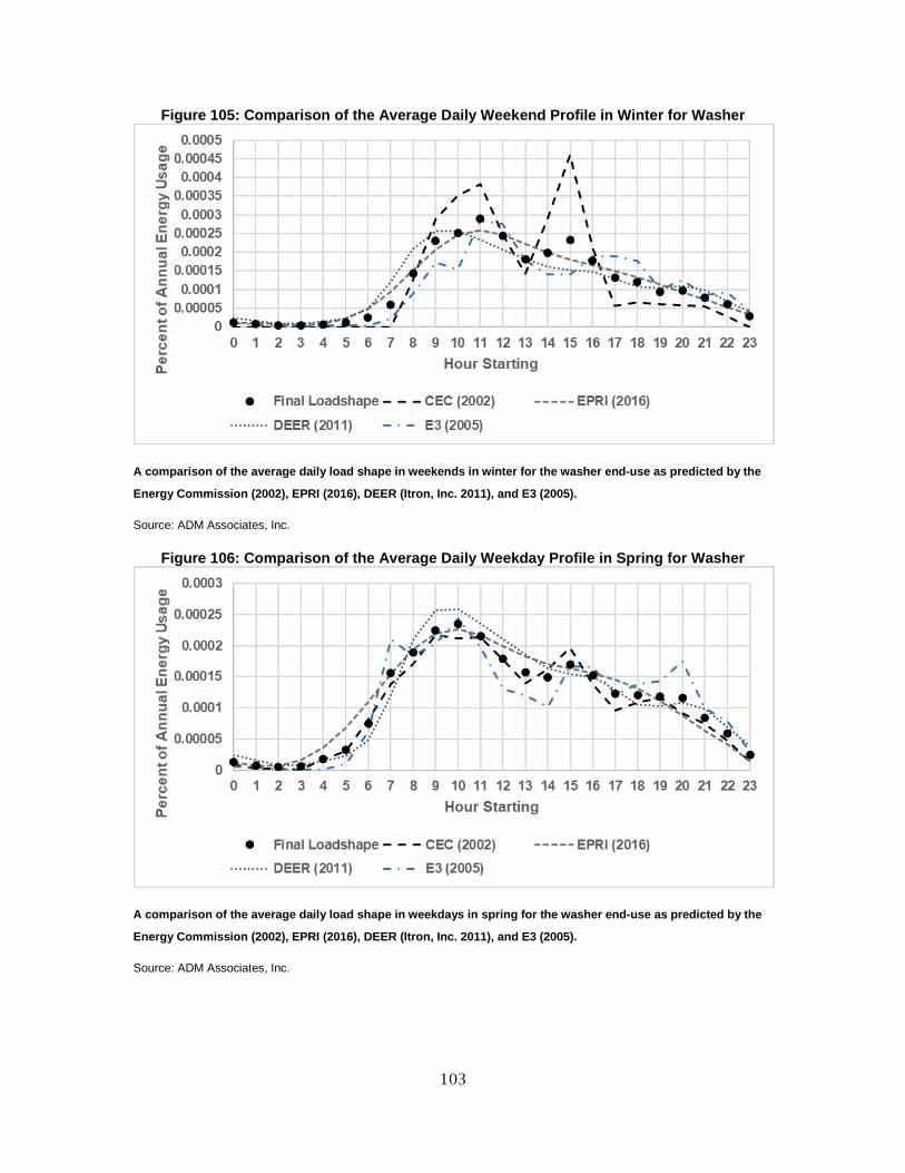
103
Figure 105: Comparison of the Average Daily Weekend Profile in Winter for Washer
A comparison of the average daily load shape in weekends in winter for the washer end-use as predicted by the
Energy Commission (2002), EPRI (2016), DEER (Itron, Inc. 2011), and E3 (2005).
Source: ADM Associates, Inc.
Figure 106: Comparison of the Average Daily Weekday Profile in Spring for Washer
A comparison of the average daily load shape in weekdays in spring for the washer end-use as predicted by the
Energy Commission (2002), EPRI (2016), DEER (Itron, Inc. 2011), and E3 (2005).
Source: ADM Associates, Inc.

104
Figure 107: Comparison of the Average Daily Weekend Profile in Spring for Washer
A comparison of the average daily load shape in weekends in spring for the washer end-use as predicted by the
Energy Commission (2002), EPRI (2016), DEER (Itron, Inc. 2011), and E3 (2005).
Source: ADM Associates, Inc.
Figure 108: Comparison of the Average Daily Weekday Profile in Summer for Washer
A comparison of the average daily load shape in weekdays in summer for the washer end-use as predicted by the
Energy Commission (2002), EPRI (2016), DEER (Itron, Inc. 2011), and E3 (2005).
Source: ADM Associates, Inc.

105
Figure 109: Comparison of the Average Daily Weekend Profile in Summer for Washer
A comparison of the average daily load shape in weekends in summer for the washer end-use as predicted by the
Energy Commission (2002), EPRI (2016), DEER (Itron, Inc. 2011), and E3 (2005).
Source: ADM Associates, Inc.
Figure 110: Comparison of the Average Daily Weekday Profile in Fall for Washer
A comparison of the average daily load shape in weekdays in fall for the washer end-use as predicted by the
Energy Commission (2002), EPRI (2016), DEER (Itron, Inc. 2011), and E3 (2005).
Source: ADM Associates, Inc.

106
Figure 111: Comparison of the Average Daily Weekend Profile in Fall for Washer
A comparison of the average daily load shape in weekends in fall for the washer end-use as predicted by the
Energy Commission (2002), EPRI (2016), DEER (Itron, Inc. 2011), and E3 (2005).
Source: ADM Associates, Inc.
Water Heating: Clothes Washer
The Energy Commission currently separates the water heating attributable to clothes
washing from other forms of water heating. ADM assumed that this load shape is
completely synonymous to the load shape for washers and therefore used that load
shape for water heating – clothes washer.
Water Heating: Dishwasher
The Energy Commission currently separates the water heating attributable to
dishwashing from other forms of water heating. ADM assumed that this load shape is
completely synonymous to the load shape for dishwashers and therefore used that load
shape for water heating – dishwasher.
Water Heating: Other
The Energy Commission distinguishes between the water heating attributable to clothes
washing, the water heating attributable to dishwashing, and all other forms of water
heating. Water heating as modeled through most sources, however, do not currently
make this distinction. The load shape from the Energy Commission’s 2002 revision also
currently includes the water heating for all three forms of water heating embedded in
the 8,760-hour load shape. ADM began the process of creating a water heating – other
load shape by first reviewing currently available sources for water heating load shapes.
After doing so, the team subtracted out the water heating attributable to clothes
washing and dishwashing from the overall water heating profile to generate a water
heating – other profile.

107
ADM reviewed three sources for water heating load shapes: the Energy Commission’s
2002 load shapes, the EPRI Load Shape Library 4.0 (2016), and the E3 Energy Efficiency
Calculator (2005). After reviewing the three data sources, the team ultimately
determined that the E3 Energy Efficiency Calculator (2005) appeared to be the most
consistent with expected behavior for water heating. Specifically, the E3 Energy
Efficiency Calculator load shape showed a reduction in energy usage in the warmer
season—which should be expected as less heat is lost due to transmission and the
starting temperature for water being heated is higher. Therefore, ADM elected to use the
E3 (2005) profile in the models. Figure 112 through
Figure 129 show the comparison between all three data sources for multifamily and
single-family homes.
Figure 112: Comparison of Monthly Energy Usage for Multifamily Water Heater Load Shape Sources
A comparison of the monthly energy usage for the multifamily water heater end-use as predicted by the Energy
Commission’s 2002 load shapes, EPRI (2016), and E3 (2005).
Source: ADM Associates, Inc.

108
Figure 113: Comparison of the Average Daily Weekday Profile in Winter for Multifamily Water Heater
A comparison of the average daily load shape in weekdays in winter for the multifamily water heater end-use as
predicted by the Energy Commission’s 2002 load shapes, EPRI (2016), and E3 (2005).
Source: ADM Associates, Inc.
Figure 114: Comparison of the Average Daily Weekend Profile in Winter for Multifamily Water Heater
A comparison of the average daily load shape in weekends in winter for the multifamily water heater end-use as
predicted by the Energy Commission’s 2002 load shapes, EPRI (2016), and E3 (2005).
Source: ADM Associates, Inc.

109
Figure 115: Comparison of the Average Daily Weekday Profile in Spring for Multifamily Water Heater
A comparison of the average daily load shape in weekdays in spring for the multifamily water heater end-use as
predicted by the Energy Commission’s 2002 load shapes, EPRI (2016), and E3 (2005).
Source: ADM Associates, Inc.
Figure 116: Comparison of the Average Daily Weekend Profile in Spring for Multifamily Water Heater
A comparison of the average daily load shape in weekends in spring for the multifamily water heater end-use as
predicted by the Energy Commission’s 2002 load shapes, EPRI (2016), and E3 (2005).
Source: ADM Associates, Inc.
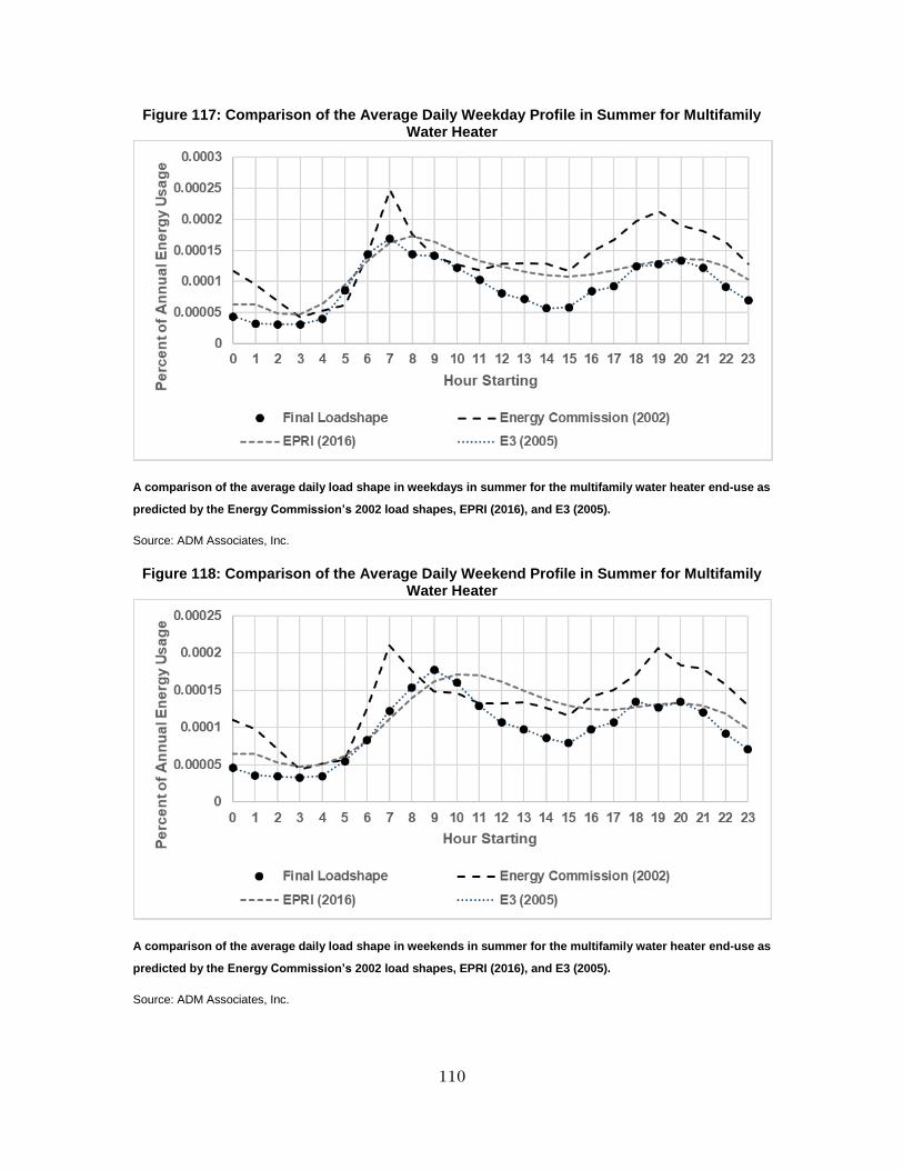
110
Figure 117: Comparison of the Average Daily Weekday Profile in Summer for Multifamily Water Heater
A comparison of the average daily load shape in weekdays in summer for the multifamily water heater end-use as
predicted by the Energy Commission’s 2002 load shapes, EPRI (2016), and E3 (2005).
Source: ADM Associates, Inc.
Figure 118: Comparison of the Average Daily Weekend Profile in Summer for Multifamily Water Heater
A comparison of the average daily load shape in weekends in summer for the multifamily water heater end-use as
predicted by the Energy Commission’s 2002 load shapes, EPRI (2016), and E3 (2005).
Source: ADM Associates, Inc.
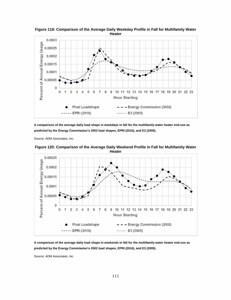
111
Figure 119: Comparison of the Average Daily Weekday Profile in Fall for Multifamily Water Heater
A comparison of the average daily load shape in weekdays in fall for the multifamily water heater end-use as
predicted by the Energy Commission’s 2002 load shapes, EPRI (2016), and E3 (2005).
Source: ADM Associates, Inc.
Figure 120: Comparison of the Average Daily Weekend Profile in Fall for Multifamily Water Heater
A comparison of the average daily load shape in weekends in fall for the multifamily water heater end-use as
predicted by the Energy Commission’s 2002 load shapes, EPRI (2016), and E3 (2005).
Source: ADM Associates, Inc.

112
Figure 121: Comparison of Monthly Energy Usage for Single-Family Water Heater Load Shape Sources
A comparison of the monthly energy usage for the single-family water heater end-use as predicted by the Energy
Commission’s 2002 load shapes, EPRI (2016), and E3 (2005).
Source: ADM Associates, Inc.
Figure 122: Comparison of the Average Daily Weekday Profile in Winter for Single-Family Water Heater
A comparison of the average daily load shape in weekdays in winter for the single-family water heater end-use as
predicted by the Energy Commission’s 2002 load shapes, EPRI (2016), and E3 (2005).
Source: ADM Associates, Inc.

113
Figure 123: Comparison of the Average Daily Weekend Profile in Winter for Single-Family Water Heater
A comparison of the average daily load shape in weekends in winter for the single-family water heater end-use as
predicted by the Energy Commission’s 2002 load shapes, EPRI (2016), and E3 (2005).
Source: ADM Associates, Inc.
Figure 124: Comparison of the Average Daily Weekday Profile in Spring for Single-Family Water Heater
A comparison of the average daily load shape in weekdays in spring for the single-family water heater end-use as
predicted by the Energy Commission’s 2002 load shapes, EPRI (2016), and E3 (2005).
Source: ADM Associates, Inc.

114
Figure 125: Comparison of the Average Daily Weekend Profile in Spring for Single-Family Water Heater
A comparison of the average daily load shape in weekends in spring for the single-family water heater end-use as
predicted by the Energy Commission’s 2002 load shapes, EPRI (2016), and E3 (2005).
Source: ADM Associates, Inc.
Figure 126: Comparison of the Average Daily Weekday Profile in Summer for Single-Family Water Heater
A comparison of the average daily load shape in weekdays in summer for the single-family water heater end-use
as predicted by the Energy Commission’s 2002 load shapes, EPRI (2016), and E3 (2005).
Source: ADM Associates, Inc.
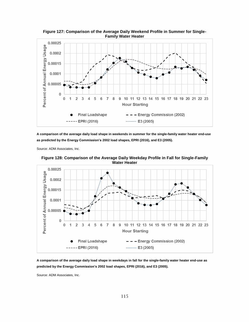
115
Figure 127: Comparison of the Average Daily Weekend Profile in Summer for Single-Family Water Heater
A comparison of the average daily load shape in weekends in summer for the single-family water heater end-use
as predicted by the Energy Commission’s 2002 load shapes, EPRI (2016), and E3 (2005).
Source: ADM Associates, Inc.
Figure 128: Comparison of the Average Daily Weekday Profile in Fall for Single-Family Water Heater
A comparison of the average daily load shape in weekdays in fall for the single-family water heater end-use as
predicted by the Energy Commission’s 2002 load shapes, EPRI (2016), and E3 (2005).
Source: ADM Associates, Inc.
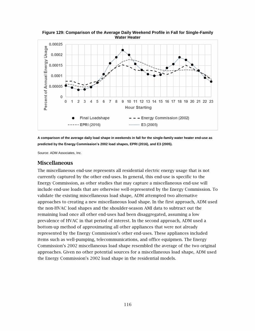
116
Figure 129: Comparison of the Average Daily Weekend Profile in Fall for Single-Family Water Heater
A comparison of the average daily load shape in weekends in fall for the single-family water heater end-use as
predicted by the Energy Commission’s 2002 load shapes, EPRI (2016), and E3 (2005).
Source: ADM Associates, Inc.
Miscellaneous
The miscellaneous end-use represents all residential electric energy usage that is not
currently captured by the other end-uses. In general, this end-use is specific to the
Energy Commission, as other studies that may capture a miscellaneous end-use will
include end-use loads that are otherwise well-represented by the Energy Commission. To
validate the existing miscellaneous load shape, ADM attempted two alternative
approaches to creating a new miscellaneous load shape. In the first approach, ADM used
the non-HVAC load shapes and the shoulder-season AMI data to subtract out the
remaining load once all other end-uses had been disaggregated, assuming a low
prevalence of HVAC in that period of interest. In the second approach, ADM used a
bottom-up method of approximating all other appliances that were not already
represented by the Energy Commission’s other end-uses. These appliances included
items such as well-pumping, telecommunications, and office equipmen. The Energy
Commission’s 2002 miscellaneous load shape resembled the average of the two original
approaches. Given no other potential sources for a miscellaneous load shape, ADM used
the Energy Commission’s 2002 load shape in the residential models.

117
Figure 130 through

118
Figure 138 present the comparison of load shapes at a monthly and average daily by
season level.

119
Figure 130: Comparison of Monthly Energy Usage for Miscellaneous Load Shape Sources
A comparison of the monthly energy usage for the miscellaneous end-use as predicted by the 2002 Energy
Commission load shape and the two original load shapes.
Source: ADM Associates, Inc.
Figure 131: Comparison of the Average Daily Weekday Profile in Winter for Miscellaneous
A comparison of the average daily load shape in weekdays in winter for the miscellaneous end-use as predicted
by the 2002 Energy Commission load shape and the two original load shapes.
Source: ADM Associates, Inc.

120
Figure 132: Comparison of the Average Daily Weekend Profile in Winter for Miscellaneous
A comparison of the average daily load shape in weekends in winter for the miscellaneous end-use as predicted
by the 2002 Energy Commission load shape and the two original load shapes.
Source: ADM Associates, Inc.
Figure 133: Comparison of the Average Daily Weekday Profile in Spring for Miscellaneous
A comparison of the average daily load shape in weekdays in spring for the miscellaneous end-use as predicted
by the 2002 Energy Commission load shape and the two original load shapes.
Source: ADM Associates, Inc.

121
Figure 134: Comparison of the Average Daily Weekend Profile in Spring for Miscellaneous
A comparison of the average daily load shape in weekends in spring for the miscellaneous end-use as predicted
by the 2002 Energy Commission load shape and the two original load shapes.
Source: ADM Associates, Inc.
Figure 135: Comparison of the Average Daily Weekday Profile in Summer for Miscellaneous
A comparison of the average daily load shape in weekdays in summer for the miscellaneous end-use as
predicted by the 2002 Energy Commission load shape and the two original load shapes.
Source: ADM Associates, Inc.
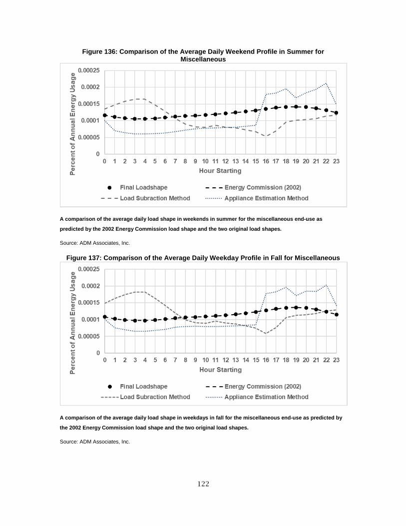
122
Figure 136: Comparison of the Average Daily Weekend Profile in Summer for Miscellaneous
A comparison of the average daily load shape in weekends in summer for the miscellaneous end-use as
predicted by the 2002 Energy Commission load shape and the two original load shapes.
Source: ADM Associates, Inc.
Figure 137: Comparison of the Average Daily Weekday Profile in Fall for Miscellaneous
A comparison of the average daily load shape in weekdays in fall for the miscellaneous end-use as predicted by
the 2002 Energy Commission load shape and the two original load shapes.
Source: ADM Associates, Inc.
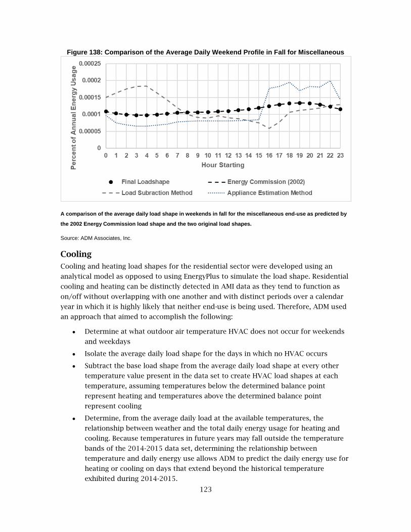
123
Figure 138: Comparison of the Average Daily Weekend Profile in Fall for Miscellaneous
A comparison of the average daily load shape in weekends in fall for the miscellaneous end-use as predicted by
the 2002 Energy Commission load shape and the two original load shapes.
Source: ADM Associates, Inc.
Cooling
Cooling and heating load shapes for the residential sector were developed using an
analytical model as opposed to using EnergyPlus to simulate the load shape. Residential
cooling and heating can be distinctly detected in AMI data as they tend to function as
on/off without overlapping with one another and with distinct periods over a calendar
year in which it is highly likely that neither end-use is being used. Therefore, ADM used
an approach that aimed to accomplish the following:
Determine at what outdoor air temperature HVAC does not occur for weekends
and weekdays
Isolate the average daily load shape for the days in which no HVAC occurs
Subtract the base load shape from the average daily load shape at every other
temperature value present in the data set to create HVAC load shapes at each
temperature, assuming temperatures below the determined balance point
represent heating and temperatures above the determined balance point
represent cooling
Determine, from the average daily load at the available temperatures, the
relationship between weather and the total daily energy usage for heating and
cooling. Because temperatures in future years may fall outside the temperature
bands of the 2014-2015 data set, determining the relationship between
temperature and daily energy use allows ADM to predict the daily energy use for
heating or cooling on days that extend beyond the historical temperature
exhibited during 2014-2015.

124
To determine at what outdoor air temperature HVAC does not occur, ADM first
calculated the average daily air temperature for each day. The average daily air
temperature was then rounded to the nearest two degrees. By rounding the average
daily air temperature in this manner, the number of potential data points at each
temperature bin is increased, therefore reducing the potential of falsely detecting a
balance point due to a lack of representative points at that given temperature. After
calculating the rounded temperature bins, the average daily load shape is then
generated by taking the average load at each hour across all days belonging to that
temperature bin. By calculating the average daily load shape, one can reduce the
volatility associated with each data point and isolate the typical building load shape at
that temperature bin.
After generating the temperature bins and average daily load shape at each temperature
bin, the balance point is then calculated by finding the temperature bin with the
minimum daily load, as calculated by summing the average daily load at each
temperature bin. The average daily load shape belonging to the temperature bin with the
minimum daily load shape is then assumed to be the base load shape. Heating and
cooling loads are then disaggregated by subtracting the base load values at each hour
from the average daily profiles from the remaining temperature bins, creating heating
and cooling load shapes at each temperature bin. Temperature bins that fall below the
balance point are considered heating temperatures and temperature bins that fall above
the balance point are considered cooling temperatures. This process is repeated once
for weekdays (Monday through Friday) and once for weekends/holidays (Saturday,
Sunday, and holidays).
The load shapes at the varying temperature bins provide some clarity as to how heating
and cooling change in shape as temperature changes. However, the extrapolation of
these load shapes is limited to the temperature with which the loads are modeled. In
this case, temperatures are limited by the observed temperature in 2014 and 2015. To
increase the generalizability of the load shapes, ADM decoupled the process of
estimating the daily energy usage (relative to the annual energy usage) from the 24-hour
profile at each temperature bin. Each 24-hour profile was normalized relative to its daily
energy usage, thus resulting in a daily energy usage totaling one per day. Relative daily
energy usage is then estimated by approximating the relationship between
heating/cooling energy use at various temperatures and HDD and CDD.
To do this, ADM calculated average daily temperatures. Unlike the daily load shapes,
ADM rounded the values to the nearest whole number instead of to the nearest two
degrees. As the project analysts regress these values in a piecewise regression, this was
done to retain data points and prevent potential over-fitting of the regression equation.
HDD and CDD were calculated using the balance point, as detected from the daily load
shape generation with an adjustment of an additional degree for CDD calculation and
less one degree for HDD calculation to account for the two-degree variance of the
detected balance point. For each HDD or CDD, the average daily cooling or heating load
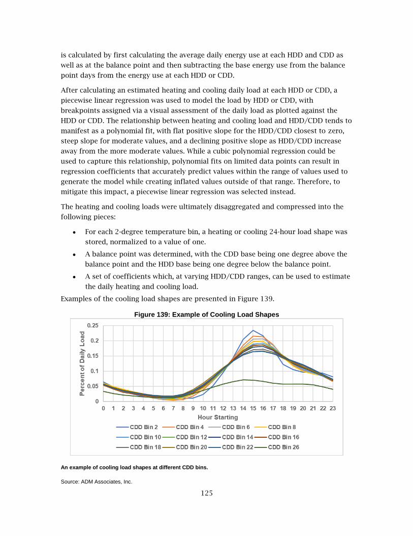
125
is calculated by first calculating the average daily energy use at each HDD and CDD as
well as at the balance point and then subtracting the base energy use from the balance
point days from the energy use at each HDD or CDD.
After calculating an estimated heating and cooling daily load at each HDD or CDD, a
piecewise linear regression was used to model the load by HDD or CDD, with
breakpoints assigned via a visual assessment of the daily load as plotted against the
HDD or CDD. The relationship between heating and cooling load and HDD/CDD tends to
manifest as a polynomial fit, with flat positive slope for the HDD/CDD closest to zero,
steep slope for moderate values, and a declining positive slope as HDD/CDD increase
away from the more moderate values. While a cubic polynomial regression could be
used to capture this relationship, polynomial fits on limited data points can result in
regression coefficients that accurately predict values within the range of values used to
generate the model while creating inflated values outside of that range. Therefore, to
mitigate this impact, a piecewise linear regression was selected instead.
The heating and cooling loads were ultimately disaggregated and compressed into the
following pieces:
For each 2-degree temperature bin, a heating or cooling 24-hour load shape was
stored, normalized to a value of one.
A balance point was determined, with the CDD base being one degree above the
balance point and the HDD base being one degree below the balance point.
A set of coefficients which, at varying HDD/CDD ranges, can be used to estimate
the daily heating and cooling load.
Examples of the cooling load shapes are presented in Figure 139.
Figure 139: Example of Cooling Load Shapes
An example of cooling load shapes at different CDD bins.
Source: ADM Associates, Inc.

126
Heating
The approach to generating the heating load shape was described in the previous sub-
section. An example of the heating load shapes is presented in Figure 140.
Figure 140: Example of Heating Load Shapes
An example of Heating load shapes at different HDD bins.
Source: ADM Associates, Inc.
Furnace Fan
Furnace fans in the residential sector typically only operate when heating or cooling is
operating. Therefore, the team assumed furnace fans to be on whenever heating or
cooling were on. To generate the load shape, the load shapes for heating and cooling are
normalized to one for a given year to weight the two profiles equally and then
aggregated together and normalized to one once more, thereby creating a normalized
furnace fan load shape. An independent furnace fan load shape was not stored as the
process of generating this load shape is dependent exclusively on the distribution of
heating and cooling in the modeled year.
Residual Load Shape The load shapes developed for the residential sector can be described as either
analytically obtained (HVAC load shapes) or obtained from the best currently available
resources (non-HVAC load shapes). Although, on an individual basis, each end-use is
relatively accurate in nature, there is still potential for variation between the modeled
end-uses and the aggregated data. Because the data represents an aggregate of all
homes belonging to a certain building-type/forecast zone, it is not readily apparent
which specific end-use causes the whole building load to deviate. It is more likely that
the deviation stems from an aggregation of minor differences between the modeled end-
uses and real-world factors.

127
Therefore, ADM developed a residual load shape. The residual load shape attempts to
recover the component of the residual that is systematic and predictable and acts as a
correction factor that attempts to bridge the gap between the modeled whole building
load and the actual whole building load by providing a relative to correction to the
modeled whole building. Unlike other load shapes, which are normalized to a total value
of one per end-use, the residual load shape is normalized as a percent correction by
diving each observation by the GWh for the base year for the given building-type and
forecast zone of interest. It can therefore be reconstituted as a function of the relative
intensity of the predicted year by multiplying the normalized profile by the modeled
year's total GWh.
ADM generated the residual load shape by taking the actual residuals (difference
between the actual AMI data and the modeled loads at each hour) and creating a series
of coefficients segmented by time-of-year (month, day-type, and hour) and regressed
against CDD and HDD. The selection of a CDD and HDD base is detailed on page 99. To
accomplish this, ADM first segmented the 8,760 data by PST or PDT period, day-type
(the 7 weekday-types plus an additional day-type for holidays), and hour. This resulted
in 384 segments of data.
ADM then ran each segment of data through the following regression model:
𝑦 = 𝛽0 + 𝛽1 ∙ 𝐶𝐷𝐷 + 𝛽2 ∙ 𝐻𝐷𝐷 + 𝜀
Where:
𝑦 is the predicted normalized residual,
𝛽0 is the intercept,
𝛽1 is the CDD weight,
𝛽2 is the HDD weight,
And 𝜀 is the error term.
By modeling the residual this, ADM have essentially captured the variability remaining
that is explainable due to temporal components and weather. Whatever residuals are
remaining are therefore discarded as random.

128
Figure 141 through

129
Figure 149 provide a comparison of the whole building load shapes with and without
application of the residual load shape.
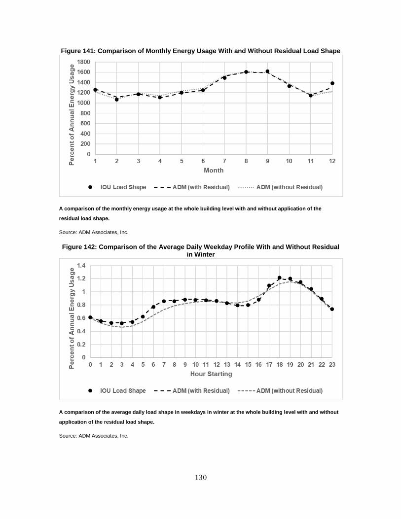
130
Figure 141: Comparison of Monthly Energy Usage With and Without Residual Load Shape
A comparison of the monthly energy usage at the whole building level with and without application of the
residual load shape.
Source: ADM Associates, Inc.
Figure 142: Comparison of the Average Daily Weekday Profile With and Without Residual in Winter
A comparison of the average daily load shape in weekdays in winter at the whole building level with and without
application of the residual load shape.
Source: ADM Associates, Inc.
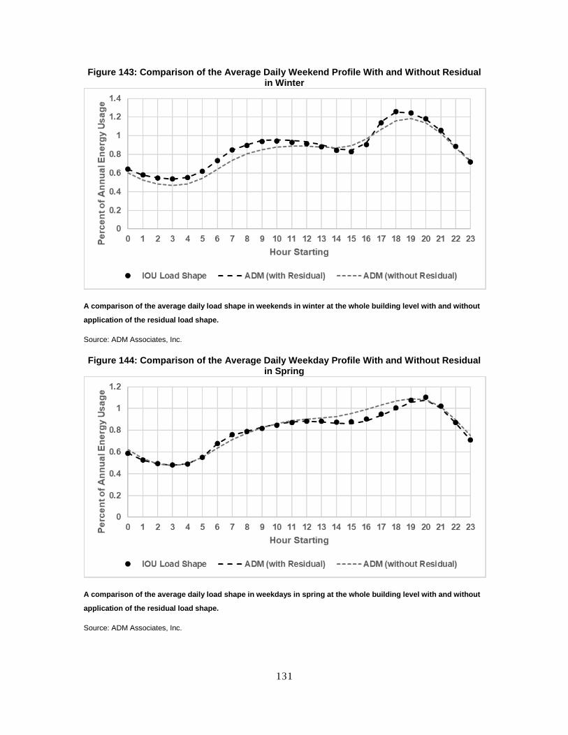
131
Figure 143: Comparison of the Average Daily Weekend Profile With and Without Residual in Winter
A comparison of the average daily load shape in weekends in winter at the whole building level with and without
application of the residual load shape.
Source: ADM Associates, Inc.
Figure 144: Comparison of the Average Daily Weekday Profile With and Without Residual in Spring
A comparison of the average daily load shape in weekdays in spring at the whole building level with and without
application of the residual load shape.
Source: ADM Associates, Inc.

132
Figure 145: Comparison of the Average Daily Weekend Profile With and Without Residual in Spring
A comparison of the average daily load shape in weekends in spring at the whole building level with and without
application of the residual load shape.
Source: ADM Associates, Inc.
Figure 146: Comparison of the Average Daily Weekday Profile With and Without Residual in Summer
A comparison of the average daily load shape in weekdays in summer at the whole building level with and
without application of the residual load shape.
Source: ADM Associates, Inc.

133
Figure 147: Comparison of the Average Daily Weekend Profile With and Without Residual in Summer
A comparison of the average daily load shape in weekends in summer at the whole building level with and
without application of the residual load shape.
Source: ADM Associates, Inc.
Figure 148: Comparison of the Average Daily Weekday Profile With and Without Residual in Fall
A comparison of the average daily load shape in weekdays in fall at the whole building level with and without
application of the residual load shape.
Source: ADM Associates, Inc.

134
Figure 149: Comparison of the Average Daily Weekend Profile With and Without Residual in Fall
A comparison of the average daily load shape in weekends in fall at the whole building level with and without
application of the residual load shape.
Source: ADM Associates, Inc.

135
CHAPTER 3: Base Load Shapes: Commercial Sector
Method and Data Sources
Method
Unlike the residential sector, which relied exclusively on a purely analytical method to
develop the load shapes, the commercial sector relies on a hybrid model which
synthesizes an analytical approach with an engineering approach. ADM relied primarily
on an analytical model to create the non-HVAC loads, however, because HVAC loads in
the commercial sector can often operate on an overlapping basis (i.e., heating and
cooling can often be operating in one facility at the same time), ADM relied on
EnergyPlus simulation models to generate the HVAC load shapes. This sub-section
provides a high-level summary of the approach to the commercial sector load shapes. A
detailed description of each step of the process is provided in further detail in later
sections of this chapter.
The Energy Commission currently divides the Commercial sector into 12 different
building-types. These 12 building-types can often include buildings that are qualitatively
different from one another within the same building-type. An example of this would be
the Restaurant building-type. Per the NAICS assignments used to determine the
Restaurant category, Restaurants can include traditional sit-down restaurants, bars, and
fast-food. These three building sub-types vary significantly in their operating schedule.
Therefore, the aggregation of these three building sub-types can lead to internal load
shapes that are difficult to craft engineering models for. Prior to requesting AMI data
from the three California IOUs, ADM divided the 12 building-types into 27 building sub-
types, with the intention of modeling non-HVAC loads on the 12 building-types and
modeling HVAC loads first on the 27 building sub-types prior to aggregating the load
shapes back to the 12 building types. Table 2 presents the 12 building-types and
corresponding building sub-types.

136
Table 2: Commercial Building-Types
Building-Type Building Sub-Type
College Academic Education
College Non-instructional educational services
College Specialized/Other Education
Food Convenience
Food Grocer
Food Specialty Food
Health Care Hospitals
Health Care Nursing and Assisted Living
Health Care Outpatient health care
Hotel Casinos
Hotel Hotels and Motels
Hotel Other lodging
Misc Data Center Like
Misc Education-Like
Misc Office-Like
Misc Other Misc
Misc Retail-Like
Office (Small/Large) Office
Refrigerated Warehouse Refrigerated Warehouse
Restaurant Bar
Restaurant Fast Food
Restaurant Other Restaurant
Restaurant Sit-Down
Retail Retail
School Educational Services
School School
Warehouse Warehouse
Presentation of the 12 building-types and corresponding building sub-types.
Source: ADM Associates, Inc.
ADM first began by sourcing new internal load shapes for non-HVAC load shapes. The
team used load shapes derived from the CEUS (Itron, Inc. 2006) the basis for the internal
load shapes. However, ADM anticipated that load shapes have shifted from the last
CEUS. In general, ADM expects that shifts in working hours and changes in equipment
efficiency will have shifted load shapes from being peaked to more distributed.
Therefore, the researchers created an analytical approach to modify the load shapes
relative to the averaged building-type AMI data the researchers received from the IOUs.
ADM performed this approach once on data corresponding to the 12 building sub-types
for use in the final base year load shapes and once on data corresponding to the 27
building sub-types for use as a basis for the engineering model internal load schedules.

137
After generating internal load schedules for each building sub-type, the schedules are
then used as the basis for the internal load schedules for the EnergyPlus simulation
models. The purpose of modifying the internal load schedules this way is to ensure that
any HVAC interactions are modeled appropriately, as opposed to using the prototypical
load shapes pre-constructed in each building model. EnergyPlus simulation models are
designed to generate outputs for single buildings. Because the goal is to create load
shapes that represent a group of buildings, the output for a single EnergyPlus
simulation model will fail to capture the true variability of the sector. Therefore, for
each of the 27 building sub-types per forecast zone, the ADM then ran a set of
EnergyPlus simulation models, varying the HVAC setpoint schedules.
Once the EnergyPlus simulation models have been created, ADM then use the building
sub-type AMI data to create a fixed regression to determine the appropriate weight of
each simulation in generating average HVAC load shapes. ADM then aggregates those
HVAC load shapes back to the 12 building-types per forecast zone based on the relative
contribution of each building sub-type to its corresponding building-type. At this point,
all end-use load shapes are compressed to a series of regression coefficients per
building-type per forecast zone. For non-HVAC coefficients, the load shapes are
compressed to 24-hour x day-type x month matrices. For HVAC coefficients, the load
shapes are compressed by either CDH or HDH x day-type x month.
After compressing the load shapes to a series of regression coefficients, ADM used the
coefficients to regenerate the load shapes for the three base years (2014-2016) and
generated the residual for each hour. This residual is then modeled using a CDH, HDH,
day-type, and month regression model to capture the systematic component of the
residual. Pieces of this newly constructed residual load shape are then used to scale the
regression coefficients for the end-use load shapes on a monthly or month x day-type
level. After adjusting the end-use load shape coefficients, a final residual load shape is
then generated.
Data Sources
The following section provides a list of the data sources used to generate the load
shapes. In addition to listing the data source, a brief description of the data source and
any data preparation activities are provided.
AMI Data
As part of this project, a data request was submitted to the three California IOUs
requesting data for all non-residential sectors from the years 2014, 2015, and 2016. In
response to this data request, the three IOUs provided averaged hourly data by building
sub-type and either usage level (PG&E and SDG&E segmented data by high, medium, and
low users) or rate class (SCE).
Prior to using the interval meter data, ADM first pre-treated all data. This pre-treatment
consisted of standardizing the nomenclature of all files and merging the dataset with
climate-zone specific hourly historical weather data obtained from the Energy

138
Commission. Hourly timestamps were standardized to units of PST for the entire year
(11 p.m. PDT was standardized to 10 p.m. PST). Data was restricted to January 1, 2014
through December 31, 2016.
As part of the data validation process, the researchers reviewed the data provided by
the IOUs. ADM data for gaps and significant spikes within the data over the year. In
some cases, ADM noticed jagged-ness, atypical gaps, or convergence of different rate
class profiles. An example of an average daily profile for each rate-class for a building-
type in a single forecast zone is presented in Figure 150.
Figure 150: Average Daily Load Shape for a Building-Type in the Commercial Sector
An example of the average daily profile for all rate classes belonging to a single building-type in a single forecast
zone in the commercial sector.
Source: ADM Associates, Inc.
As seen in the plot, the load shapes for one of the general services rate classes (GS-2),
and two of the time-of-use rates (TOU-8 and TOU-GS-3) bear a strong resemblance to
one another. However, the profiles for agriculture and pumping (AG & PUMP) and one of
the general services rates (GS-1) show atypical patterning in that both have unexpected
drops at specific hours. Furthermore, the intensity of the AG & PUMP shape is
significantly higher than the other load shapes (and, consequently, lower in other
months). The underlying cause of these patterns can be attributed to multiple causes,
such as changing of rate class for some meters over the year, or misattribution of sub-
meters to a specific rate class.
Because ADM cannot assume that these types of anomalies are attributable to data
artifacts, ADM blended the profiles for each building sub-type across rate class. The
result of blending the rate class level load data from Figure 150 as shown in

139
Figure 151.

140
Figure 151: Average Daily Load Shape for a Building-Type in the Commercial Sector Post-Aggregation
An example of the average daily profile after aggregating across rate classes for a single building-type in a single
forecast zone in the commercial sector.
Source: ADM Associates, Inc.
As can be seen, aggregating the different rate classes together generates a load shape
that reduces the anomalies attributable to any given rate class load shape. Although the
example shown illustrates this process for data sets segmented by rate class, these
patterns also exist in the data sets that were segmented by usage level. Therefore, all
data segments per building sub-type per forecast zone were aggregated together.
Commercial Building Energy Demand Forecast Model
The Commercial Building Energy Demand Forecast Model is the component of the CED
Model that predicts the overall annual energy usage for a given end-use at the forecast
zone level. The predicted GWh is further subdivided by building type. For example, the
model has predictions of the total annual interior lighting GWh for all colleges in
forecast zone 1. Updates are made to the model on an annual basis, with major
revisions occurring bi-annually. The Energy Commission corrects its historical load
forecast based on observed whole-building energy use on an annual basis, thereby
adjusting the end-use level forecast based on the total observed load.
As part of the process of developing load shapes for the base years of 2014, 2015 and
2016, ADM leveraged the weather-adjusted forecast values from the Commercial
Building Energy Demand Forecast Model for 2014, 2015 and 2016 and assumed that the
overall energy usage per end-use was distributed in the same proportions as the model.

141
Weather Data
An extract of weather data was supplied by the Energy Commission for 2014-2016.
Weather data consisted of outdoor air temperature, dew point, precipitation, windspeed,
wind direction, total sky cover, and mean sea level pressure. Weather files were
generated for all major AWS in California. The Energy Commission provided weighting
files meant to define the appropriate weighting of each AWS to generate a forecast-zone-
level weather file.
California Commercial End-Use Survey
The most recent CEUS was published in 2006 by Itron, Inc. and provides information
regarding the total floor stock, energy intensity, and percent energy distribution for 13
different end-uses. Additionally, the 2006 CEUS provides 8,760 load shapes per end-use.
The end-uses captured in the 2006 CEUS were:
Air compressor
Cooking
Cooling
Exterior lighting
Heating
Interior lighting
Miscellaneous
Motors
Office equipment
Process
Refrigeration
Ventilation
Water heating
Results were presented by building type, forecast zone, and utility company. Forecast
zones use a stale-dated scheme of ten forecast zones for the three IOUs. The Energy
Commission currently uses a 12-forecast zone schematic, therefore, the ADM reviewed
data at a building type by utility company level.
Pre-Simulation Modeling Although ADM has sourced new end-use load shapes from the CEUS (Itron, Inc. 2006),
there may still be differences in the load shapes in the current base period of 2014-2016
compared to the 2005 base year used by the CEUS.

142
Figure 152 provides a hypothetical example of an average daily profile in 2005
compared to an average daily profile in 2014-2016.

143
Figure 152: Example Comparison of a Whole Building Load in 2005 vs. 2015-2016
Hypothetical comparison of a daily load shape in a building in 2005 compared to a building in 2014-2016.
Source: ADM Associates, Inc.
In general, one can anticipate that the energy use in 2014-2016 has reduced, on average,
due to changes in building code and improved energy efficiency. In addition, the peak of
the curve is not as pronounced in 2014-2016 relative to 2005. This assumption can be
made because the energy efficiency improvements between 2005 and 2014-2016 are
likely to be lighting and office equipment-based improvements, which will reduce the
relative impact of lighting compared to the other end-use loads and consequently
minimize interactive effects in HVAC loads.
Additionally, the load shapes from CEUS, as well as the GWhs predicted by the
Commercial Building Energy Demand Forecast Model, are generated at a higher level
than the building types used by ADM. For example, restaurants have been broken down
into several sub-types for the purpose of this study. Therefore, ADM needed to adapt
the load shapes from the 2006 CEUS to match changes in 2014-2016 due to shifts in
energy efficiency and match the load shapes to the building sub-type from the original
building type.
To adapt the load shapes, ADM used the following approach:
1. For a given building sub-type in a given forecast zone, project analysts selected
the corresponding major building-type end-use load shapes for the same IOU
from the 2006 CEUS—because forecast zones were redesigned between the time
of the last CEUS and present day, were not able map the load shapes at a more
granular, forecast zone resolution.
2. Outdoor lighting load shapes were developed independently based on historical
sunrise/sunset data. Outdoor lighting was then subtracted from the IOU data

144
based on its relative weight as predicted from the Commercial Building Energy
Demand Forecast Model.
3. After selecting the appropriate load shape, ADM used the annual demand per
end-use for the major building type for that specific forecast zone as predicted
by the Commercial Building Energy Demand Forecast Model to estimate the
relative weight of each end-use load shape for that building type and forecast
zone. The load shapes were then scaled appropriately. Non-HVAC loads were
then aggregated to generate an estimate of the 2014 whole-building load shape
in absentia of HVAC related loads.
4. The IOU load shape for 2014 and the CEUS-based load shape were normalized,
and February was isolated as the "base month." This is because February showed
the least amount of weather-dependence upon exploratory analysis, suggesting a
limited impact of HVAC in this month.
5. After isolating February for the IOU load shape and the CEUS-based load shape,
the project team ran an hour-matching algorithm. This hour-matching algorithm
looked at every hour in the IOU load shape relative to its percent of peak in that
same day and found its closest match in the corresponding weekday types in the
CEUS data. For example, for 1 a.m. Monday, February 3, 2014, the algorithm
looked at all Mondays in the CEUS load shape and found the hour it most closely
resembled across all Mondays of the CEUS load shape.

145
6. Table 3 provides an example of ADM's hour-matching algorithm for a sample 24-
hour period.
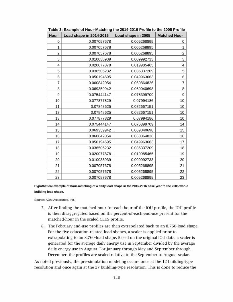
146
Table 3: Example of Hour-Matching the 2014-2016 Profile to the 2005 Profile
Hour Load shape in 2014-2016 Load shape in 2005 Matched Hour
0 0.007057678 0.005268895 0
1 0.007057678 0.005268895 1
2 0.007057678 0.005268895 2
3 0.010038939 0.009992733 3
4 0.020077878 0.019985465 4
5 0.036505232 0.036337209 5
6 0.050194695 0.049963663 6
7 0.060842054 0.060864826 7
8 0.069359942 0.069040698 8
9 0.075444147 0.075399709 9
10 0.077877829 0.07994186 10
11 0.07848625 0.082667151 10
12 0.07848625 0.082667151 10
13 0.077877829 0.07994186 10
14 0.075444147 0.075399709 14
15 0.069359942 0.069040698 15
16 0.060842054 0.060864826 16
17 0.050194695 0.049963663 17
18 0.036505232 0.036337209 18
19 0.020077878 0.019985465 19
20 0.010038939 0.009992733 20
21 0.007057678 0.005268895 21
22 0.007057678 0.005268895 22
23 0.007057678 0.005268895 23
Hypothetical example of hour-matching of a daily load shape in the 2015-2016 base year to the 2005 whole
building load shape.
Source: ADM Associates, Inc.
7. After finding the matched-hour for each hour of the IOU profile, the IOU profile
is then disaggregated based on the percent-of-each-end-use present for the
matched-hour in the scaled CEUS profile.
8. The February end-use profiles are then extrapolated back to an 8,760-load shape.
For the five education-related load shapes, a scaler is applied prior to
extrapolating to an 8,760-load shape. Based on the original IOU data, a scaler is
generated for the average daily energy use in September divided by the average
daily energy use in August. For January through May and September through
December, the profiles are scaled relative to the September to August scalar.
As noted previously, the pre-simulation modeling occurs once at the 12 building-type
resolution and once again at the 27 building-type resolution. This is done to reduce the
147
number of manipulations are necessary to generate the final load shapes. ADM’s goal is
to ultimately generate load shapes for the 12 building-types that are used by the Energy
Commission in the CED Model. By segmenting the profile into its 27 building sub-types,
using those profiles in the EnergyPlus models, and then aggregating the end-use profiles
to their original 12 building-types, one introduces multiple points at which the profiles
may change or shift due to data restructuring or manipulation. By running the process
twice, ADM can ensure that appropriate schedules feed into the EnergyPlus models
while still retaining unaltered profiles for the 12 building-types.
Parametric EnergyPlus Models To capture the interactive effects of HVAC loads in the commercial sector, ADM used
EnergyPlus simulations to generate HVAC load shapes (Table 4). The EnergyPlus models
were sourced from The U.S. Department of Energy (DOE) Commercial Prototype Building
Models (Pacific Northwest National Laboratory 2018). The prototype models include 12
commercial building types which were used to develop the 27 building sub-types per
forecast zone. ADM’s calibration process involved modeling various circumstances that
encompass most scenarios, where each scenario differed by the selected variable’s
magnitudes. The magnitude of specific variables was modified via parametric
processing where the framework of the model could remain static. This allowed ADM to
see the effects of modifying each specific variable. Using the parametric functionality
also allowed the ADM to scale up the total number of models and variables which
increased dramatically when simulating 27 building sub-types in each weather
forecasting zone with several parametric variables each.
Table 4: Example Parametric Combination Matrix
Magnitude Interactions
Variable #1
High Medium Low
Vari
ab
le #
2
High Run #1 Run #2 Run #3
Medium Run #4 Run #5 Run #6
Low Run #7 Run #8 Run #9
Example of how parametric combinations result in different EnergyPlus runs used by ADM in load shape
development.
Source: ADM Associates, Inc.
Parametric functionality in EnergyPlus allowed ADM to efficiently and reliably create
and simulate numerous results, but the dramatic increase in results compared to
variables resulted in the need for batch runs using R.

148
Batch Runs Through R/EnergyPlus Integration The programming language R is used to control EnergyPlus. Although R is usually used
for data handling and statistical modeling, it is also suitable as a scripting language for
developing input files and automating many tasks which could not be done manually at
this scale. One of the reasons EnergyPlus was selected as the simulation tool is because
it can be run from the command line as an executable, and the input files can be
modified extensively without intermediate software. This flexibility enabled ADM to
scale building simulation to the thousands of runs required to generate load shapes at
this level of detail.
Approximately 40 R scripts were written to complete the operations needed to run
EnergyPlus to develop load shapes. Some of the major operations included:
Create EnergyPlus weather file
Update input files to use end-use coefficients from the pre-simulation model
Generate setpoint schedules for the HVAC subsystems
Run EnergyPlus Parametric pre-processor to develop individual runs with various
physical parameters and schedules
Produce batch file by climate zone to run EnergyPlus models at scale
Map prototypical buildings to represent building subcategories used for load
shapes
These scripts were managed in a code repository and used industry standard R best
practices where possible to make iterations rapid and improve code durability.
Calibration for Commercial Models Because the AMI data provided by the IOUs is aggregated in nature, it is unlikely that
any given simulation will be able to accurately represent the overarching load shape for
an entire sector. This is because simulation models represent load shapes as discrete
operating schedules. While this would be true of an individual building, at an aggregated
level, load shapes shift from discrete to continuous in nature because some portion of
the population of interest will still be contributing to that end-use load at less common
times. For example, 7 a.m. on a summer day would most likely only have a small
proportion of all buildings using central air conditioner. However, a simulation model
may assume that the end-use is completely off during that period.
The parametric simulations encompass varying circumstances that account for most
scenarios. Therefore, each simulation represents some proportion of the underlying
population, although the relative weight of each simulation in its contribution to the
population-level load is unknown. Instead of attempting to select a single simulation
model that best encapsulates the population-level AMI data, the goal through calibration
was to approximate the percent to which each simulation model contributes to the
population.

149
To accomplish this goal, ADM relied on linear optimization via a constrained regression
model. The constraints placed on the regression aim to replicate two real-world
assumptions:
1. There is no "intercept" term because the aggregated AMI-load shape should be
fully encompassed in the parametric simulations.
2. Although the impact of a given parametric simulation can be 0, it cannot
contribute negatively to the overall load.
The regression model for the calibration is specified as follows:
𝑘𝑊ℎ𝐴𝑀𝐼 = ∅ + 𝛽1 ∙ 𝐸𝑛𝑒𝑟𝑔𝑦𝑃𝑙𝑢𝑠1 + ⋯ + 𝛽𝑛 ∙ 𝐸𝑛𝑒𝑟𝑔𝑦𝑃𝑙𝑢𝑠𝑛
Where:
𝑘𝑊ℎ𝐴𝑀𝐼 is the billing data load
∅ is a fixed intercept term of 0
𝛽1 is the weight of the first EnergyPlus run
𝛽𝑛 is the weight of the last EnergyPlus run
ADM anticipated that some of the parametric simulation models may overlap and be
collinear to one another. In an unconstrained regression, this can result in
compensatory weighting in which one independent variable may be extremely negative
while another becomes extremely positive. However, by constraining the regression, one
can assume that the variability associated with the two models will either distribute
themselves randomly amongst the two models, or one model will be weighted as 0 while
the other model retains the full weight attributable to both models. Therefore, ADM was
not concerned about either phenomenon occurring as collinearity between two models
suggests that either model can explain both simulation parameters sufficiently well.
After determining the relative weight of each simulation model, the load shapes for all
simulation models were blended together in the relative proportion as determined by
the regression coefficients.
Post Calibration Modeling The post-calibration modeling primarily consisted of compressing the three HVAC loads
(cooling, heating, and ventilation) to a series of predictive coefficients that can be used
to generate these load shapes in periods outside of the 2014 base year. As noted
previously, the seven non-HVAC loads were compressed at a month x hour resolution as
part of the process of modifying the CEUS (Itron, Inc. 2006) load shapes into predictive
load shapes for the 2014 base year for the 27 building sub-types and for the 12 building
types used by the Energy Commission.
Dividing the 12 Energy Commission building types into further building sub-types
facilitated EnergyPlus simulations, as the impact of efficiency measures can have
significant differences on buildings that may be categorized in the same building type
but are functionally different (for example, an outpatient health care facility versus a

150
hospital). However, ADM are ultimately concerned with consolidating those impacts
back into the 12 building types used by the CED Model. Therefore, after consolidating
the EnergyPlus runs into a single run per building sub-type per forecast zone using the
calibration weights, ADM then consolidated from the 27 building sub-types to the 12
Energy Commission building types using weighting files provided by the three IOUs as
part of their fulfillment of the data request. What results are load shapes that
approximate the average load shape for all buildings of a given building type in a
forecast zone.
ADM first began by normalizing the heating, cooling, and ventilation load shapes to an
annual sum of one per load. After normalizing the load shapes, the AD< then segmented
the data by PST/PDT, day-type, and hour. Although ADM could model the three-way
interaction of PST/PDT, day-type, and hour in one consolidated regression, doing so
would result in the regression exceeding the bounds of normal computing resources.
Segmenting the data set allows for the arrival at a mathematically identical result while
conserving computing resources. CDH and HDH values were generated for each data set
using the appropriate hourly weather data. Each data segment was then run through a
simple weather-based linear regression.
The regression model for cooling is specified as follows:
𝑦 = 𝛽0 + 𝛽1 ∙ 𝐶𝐷𝐻 + 𝜀
Where:
y is the modeled cooling load for a given hour
𝛽0 is the intercept
𝛽1 is the CDH weight
𝜀 is the model error
The regression model for heating is specified as follows:
𝑦 = 𝛽0 + 𝛽1 ∙ 𝐻𝐷𝐻 + 𝜀
Where:
y is the modeled heating load for a given hour
𝛽0 is the intercept
𝛽1 is the HDH weight
𝜀 is the model error
The regression model for ventilation is specified as follows:
𝑦 = 𝛽0 + 𝛽1 ∙ 𝐶𝐷𝐻 + 𝛽2 ∙ 𝐻𝐷𝐻 + 𝜀
Where:
y is the modeled ventilation load for a given hour
𝛽0 is the intercept
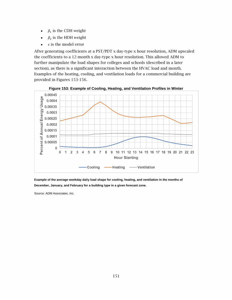
151
𝛽1 is the CDH weight
𝛽2 is the HDH weight
𝜀 is the model error
After generating coefficients at a PST/PDT x day-type x hour resolution, ADM upscaled
the coefficients to a 12-month x day-type x hour resolution. This allowed ADM to
further manipulate the load shapes for colleges and schools (described in a later
section), as there is a significant interaction between the HVAC load and month.
Examples of the heating, cooling, and ventilation loads for a commercial building are
provided in Figures 153-156.
Figure 153: Example of Cooling, Heating, and Ventilation Profiles in Winter
Example of the average weekday daily load shape for cooling, heating, and ventilation in the months of
December, January, and February for a building type in a given forecast zone.
Source: ADM Associates, Inc.

152
Figure 154: Example of Cooling, Heating, and Ventilation Profiles in Spring
Example of the average weekday daily load shape for cooling, heating, and ventilation in the months of
December, January, and February for a building type in a given forecast zone.
Source: ADM Associates, Inc.
Figure 155: Example of Cooling, Heating, and Ventilation Profiles in Summer
Example of the average weekday daily load shape for cooling, heating, and ventilation in the months of
December, January, and February for a building type in a given forecast zone.
Source: ADM Associates, Inc.
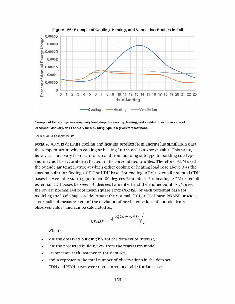
153
Figure 156: Example of Cooling, Heating, and Ventilation Profiles in Fall
Example of the average weekday daily load shape for cooling, heating, and ventilation in the months of
December, January, and February for a building type in a given forecast zone.
Source: ADM Associates, Inc.
Because ADM is deriving cooling and heating profiles from EnergyPlus simulation data,
the temperature at which cooling or heating “turns on” is a known value. This value,
however, could vary from run-to-run and from building sub-type to building sub-type
and may not be accurately reflected in the consolidated profiles. Therefore, ADM used
the outside air temperature at which either cooling or heating load rose above 0 as the
starting point for finding a CDH or HDH base. For cooling, ADM tested all potential CDH
bases between the starting point and 80 degrees Fahrenheit. For heating, ADM tested all
potential HDH bases between 50 degrees Fahrenheit and the ending point. ADM used
the lowest normalized root mean square error (NRMSE) of each potential base for
modeling the load shapes to determine the optimal CDH or HDH base. NRMSE provides
a normalized measurement of the deviation of predicted values of a model from
observed values and can be calculated as:
𝑁𝑅𝑀𝑆𝐸 = √(∑ (𝑥𝑖 − 𝑦𝑖)2𝑛
𝑖 )𝑛⁄
�̅�⁄
Where:
x is the observed building kW for the data set of interest,
y is the predicted building kW from the regression model,
i represents each instance in the data set,
and n represents the total number of observations in the data set.
CDH and HDH bases were then stored in a table for later use.

154
Residual Load Shape Although the parametric simulations encompass most scenarios underlying the
aggregated AMI data provided by the IOUs, there is still potential for variation between
the final, calibrated models and the aggregated AMI data. Because the data represents
an aggregate of all buildings belonging to a certain building-type/forecast zone, it is not
readily apparent which specific end-use causes the simulation model to deviate. It is
more likely that the deviation stems from an aggregation of minor differences between
the modeled load shapes and real-world factors.
Therefore, ADM developed a residual load shape. The residual load shape attempts to
recover the component of the residual that is systematic and predictable and acts as a
correction factor that attempts to bridge the gap between the modeled whole building
load and the actual whole building load by providing a relative to correction to the
modeled whole building. Unlike other load shapes, which are normalized to a total value
of one per end-use, the residual load shape is normalized as a percent correction by
diving each observation by the GWh for the base year for the given building-type and
forecast zone of interest. It can therefore be reconstituted as a function of the relative
intensity of the predicted year by multiplying the normalized profile by the modeled
year's total GWh.
ADM generated the residual load shape by taking the actual residuals (difference
between the actual AMI data and the modeled loads at each hour) and creating a series
of coefficients segmented by time-of-year (month, day-type, and hour) and regressed
against CDH and HDH.4. To accomplish this, ADM first segmented the 8,760 data by
month, day-type (the seven weekday-types plus an additional day-type for holidays), and
hour.
ADM then ran each segment of data through the following regression model:
𝑦 = 𝛽0 + 𝛽1 ∙ 𝐶𝐷𝐻 + 𝛽2 ∙ 𝐻𝐷𝐻 + 𝜀
Where:
𝑦 is the predicted normalized residual
𝛽0 is the intercept
𝛽1 is the CDH weight
𝛽2 is the HDH weight
𝜀 is the model error
4 The selection of a CDD and HDD base is detailed in the “Post Calibration Modeling” section beginning on page 118

155
By modeling the residual this, ADM has essentially captured the variability remaining
that is explainable due to temporal components and weather. Whatever residuals are
remaining are therefore discarded as random.
Figure 157 through
Figure 165 provide a comparison of the whole building load shapes with and without
application of the residual load shape.
Figure 157: Comparison of Monthly Energy Usage With and Without Residual Load Shape
A comparison of the monthly energy usage at the whole building level with and without application of the
residual load shape.
Source: ADM Associates, Inc.
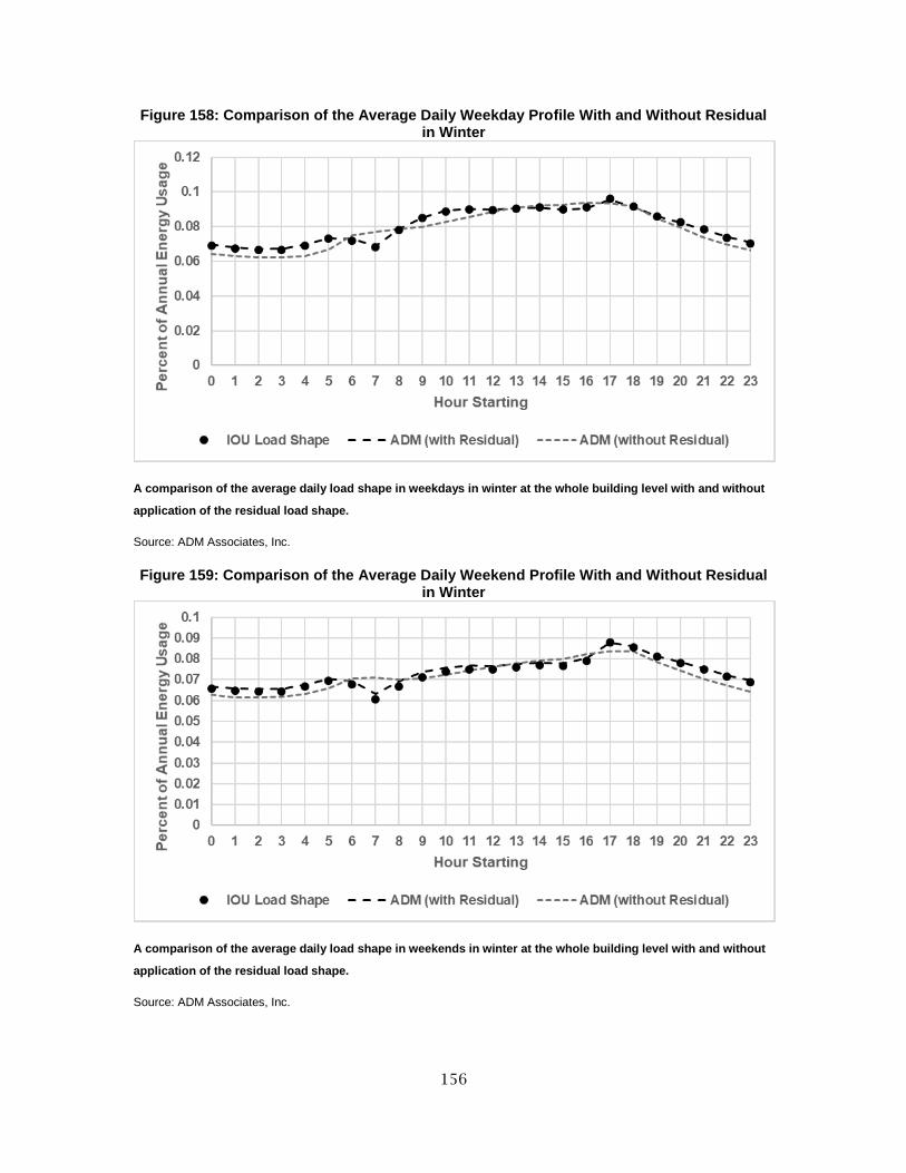
156
Figure 158: Comparison of the Average Daily Weekday Profile With and Without Residual in Winter
A comparison of the average daily load shape in weekdays in winter at the whole building level with and without
application of the residual load shape.
Source: ADM Associates, Inc.
Figure 159: Comparison of the Average Daily Weekend Profile With and Without Residual in Winter
A comparison of the average daily load shape in weekends in winter at the whole building level with and without
application of the residual load shape.
Source: ADM Associates, Inc.
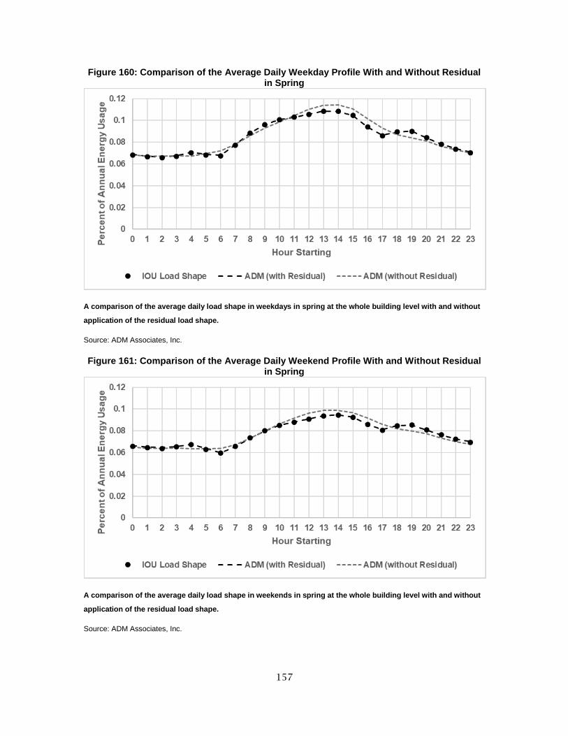
157
Figure 160: Comparison of the Average Daily Weekday Profile With and Without Residual in Spring
A comparison of the average daily load shape in weekdays in spring at the whole building level with and without
application of the residual load shape.
Source: ADM Associates, Inc.
Figure 161: Comparison of the Average Daily Weekend Profile With and Without Residual in Spring
A comparison of the average daily load shape in weekends in spring at the whole building level with and without
application of the residual load shape.
Source: ADM Associates, Inc.

158
Figure 162: Comparison of the Average Daily Weekday Profile With and Without Residual in Summer
A comparison of the average daily load shape in weekdays in summer at the whole building level with and
without application of the residual load shape.
Source: ADM Associates, Inc.
Figure 163: Comparison of the Average Daily Weekend Profile With and Without Residual in Summer
A comparison of the average daily load shape in weekends in summer at the whole building level with and
without application of the residual load shape.
Source: ADM Associates, Inc.

159
Figure 164: Comparison of the Average Daily Weekday Profile With and Without Residual in Fall
A comparison of the average daily load shape in weekdays in fall at the whole building level with and without
application of the residual load shape.
Source: ADM Associates, Inc.
Figure 165: Comparison of the Average Daily Weekend Profile With and Without Residual in Fall
A comparison of the average daily load shape in weekends in fall at the whole building level with and without
application of the residual load shape.
Source: ADM Associates, Inc.

160
Adjustments for Schools/Colleges Unlike the ten other commercial building types, colleges and schools generally do not
operate on a year-round basis. This reduced operation is apparent when reviewing the
AMI data in a given forecast zone.
Figure 166 provides an example of the average daily energy use for colleges in a given
forecast zone in the year 2014. The average daily energy use significantly reduces in the
summer months, although summer in other commercial building types is typically
hallmarked by higher energy use due to the presence of cooling load.
Figure 166: Example of Average Daily GWh by Month in Colleges
An example of the average daily GWh by month for all colleges in a single forecast zone.
Source: ADM Associates, Inc.
Although the daily profiles in the summer months represent a reduction in sector-level
energy use, ADM cannot attribute this reduction solely to the absence of end-use loads
altogether. Rather, because ADM is modeling the average profile across all buildings in a
given forecast zone, there will still be a portion of buildings active and contributing to
the load during these periods of low energy use. Additionally, although EnergyPlus has
the capacity to model accurate load shapes relative to a specified weather profile, it is
difficult to model load shapes in the summer months as the change in the load shape in
the summer month is more or less a reduction in the intensity of the curve rather than a
change in the cooling set point schedule, which would ultimately reduce the summer
load by changing the cooling profile instead of keeping its profile and reducing its
magnitude.
Therefore, ADM elected to adjust the intensity of the heating, cooling, and ventilation
load shapes for colleges and schools analytically instead of adjusting them as part of
the EnergyPlus framework. ADM first began by generating 8,760 load shapes for the

161
non-HVAC loads using the end-use load shapes.5 These load shapes were then scaled
according to the 2014, 2015, and 2016 GWh specified in the Commercial Building Energy
Demand Forecast Model. Similarly, the AMI data for each building type for each year for
each forecast zone was scaled to the corresponding total GWh for 2014, 2015, and 2016,
respectively. ADM then took the difference between the scaled AMI data and the
modeled non-HVAC end-uses. This difference was assumed to be the energy usage
attributable to the three HVAC loads. ADM used this baseline-subtracted HVAC load
shape to create a series of scalars with which ADM could then increase or decrease the
intensity of the EnergyPlus-modeled HVAC load shapes.
To begin doing this, ADM generated 8,760 load shapes for heating, cooling, and
ventilation for 2014, 2015, and 2016 using the smoothed and compressed coefficients.6
These profiles were scaled to their respective GWh values as predicted by the
Commercial Building Energy Demand Forecast Model and aggregated together to create
an overall “HVAC” load shape for 2014, 2015, and 2016. ADM aggregated across the
three HVAC load shapes because ADM could not assume which proportion of the
baseline-subtracted HVAC load belongs to each of the three end-uses. Additionally,
there is significant overlap between the heating and cooling season in commercial space,
as cooling will tend to run all year round while heating will be isolated to a specific time
of year. Therefore, to maintain a conservative approach, ADM created scalars for HVAC
aggregated across heating, cooling, and ventilation and applied the same scalars to all
three load shapes.
The baseline-subtracted HVAC profile provides several avenues for potentially
correcting the modeled HVAC load shapes. ADM now has a baseline-subtracted HVAC
profile at an 8,760 resolution. Although ADM could use said profile to make 8,760-level
adjustments to the heating, cooling, and ventilation load shapes, there is a margin of
error associated with each observation in the 8,760-load shape. If ADM assumes that
this error is distributed randomly across the 8,760 profile, the margin of error for a
single point estimation should reduce as ADM works in higher resolutions. Thus, while
error persist at an hourly resolution, that error should begin to cancel itself out as
higher resolutions of data are reviewed such as at a daily level, etc. Furthermore,
although ADM could manipulate the heating, cooling, and ventilation load shapes
relative to the 8,760 baseline-subtracted profile, ADM cannot know the relationship in
the 8,760 baseline-subtracted profile and the three underlying end-uses and modifying
the modeled end-uses may result in inappropriate changes to the load shapes.
As a compromise, ADM created scalars that changed the intensity of the modeled load
shapes compared to the baseline-subtracted profiles at a month by weekday level. To
5 The generation of the HVAC coefficients is detailed in the “Post Calibration Modeling” section beginning on page 118.

162
create these scalars, ADM aggregated the baseline-subtracted profiles and the modeled
HVAC profile by taking the sum of the GWh for each month and weekday/weekend. A
scalar was then generated by dividing the baseline-subtracted GWh values by the
corresponding modeled HVAC GWh. This results in a series of 24 scalars that can then
be used to modify the coefficients stored for the heating, cooling, and ventilation load
shapes. ADM then reviewed the scalars for each building and made additional
adjustments to the monthly intensity of HVAC and non-HVAC loads when deemed
appropriate.
Figure 167 through Figure 175 provide examples of a school in a given forecast zone
with and without scalar adjustment.
Figure 167: Comparison of Monthly Energy Usage With and Without Scalar Adjustments
A comparison of the monthly energy usage at the whole building level with and without application of the month
x day scalars but prior to application of the residual load shape.
Source: ADM Associates, Inc.

163
Figure 168: Average Daily Weekday Profile With and Without Scalar Adjustments in Winter
A comparison of the average daily load shape in weekdays in winter at the whole building level with and without
application of the month x day scalars but prior to application of the residual load shape.
Source: ADM Associates, Inc.
Figure 169: Average Daily Weekend Profile With and Without Scalar Adjustments in Winter
A comparison of the average daily load shape in weekends in winter at the whole building level with and without
application of the month x day scalars but prior to application of the residual load shape.
Source: ADM Associates, Inc.

164
Figure 170: Average Daily Weekday Profile With and Without Scalar Adjustments in Spring
A comparison of the average daily load shape in weekdays in spring at the whole building level with and without
application of the month x day scalars but prior to application of the residual load shape.
Source: ADM Associates, Inc.
Figure 171: Average Daily Weekend Profile With and Without Scalar Adjustments in Spring
A comparison of the average daily load shape in weekends in spring at the whole building level with and without
application of the month x day scalars but prior to application of the residual load shape.
Source: ADM Associates, Inc.

165
Figure 172: Average Daily Weekday Profile With and Without Scalar Adjustments in Summer
A comparison of the average daily load shape in weekdays in summer at the whole building level with and
without application of the month x day scalars but prior to application of the residual load shape.
Source: ADM Associates, Inc.
Figure 173: Average Daily Weekend Profile With and Without Scalar Adjustments in Summer
A comparison of the average daily load shape in weekends in summer at the whole building level with and
without application of the month x day scalars but prior to application of the residual load shape.
Source: ADM Associates, Inc.

166
Figure 174: Average Daily Weekday Profile With and Without Scalar Adjustments in Fall
A comparison of the average daily load shape in weekdays in fall at the whole building level with and without
application of the month x day scalars but prior to application of the residual load shape.
Source: ADM Associates, Inc.
Figure 175: Average Daily Weekend Profile With and Without Scalar Adjustments in Fall
A comparison of the average daily load shape in weekends in fall at the whole building level with and without
application of the month x day scalars but prior to application of the residual load shape.
Source: ADM Associates, Inc.
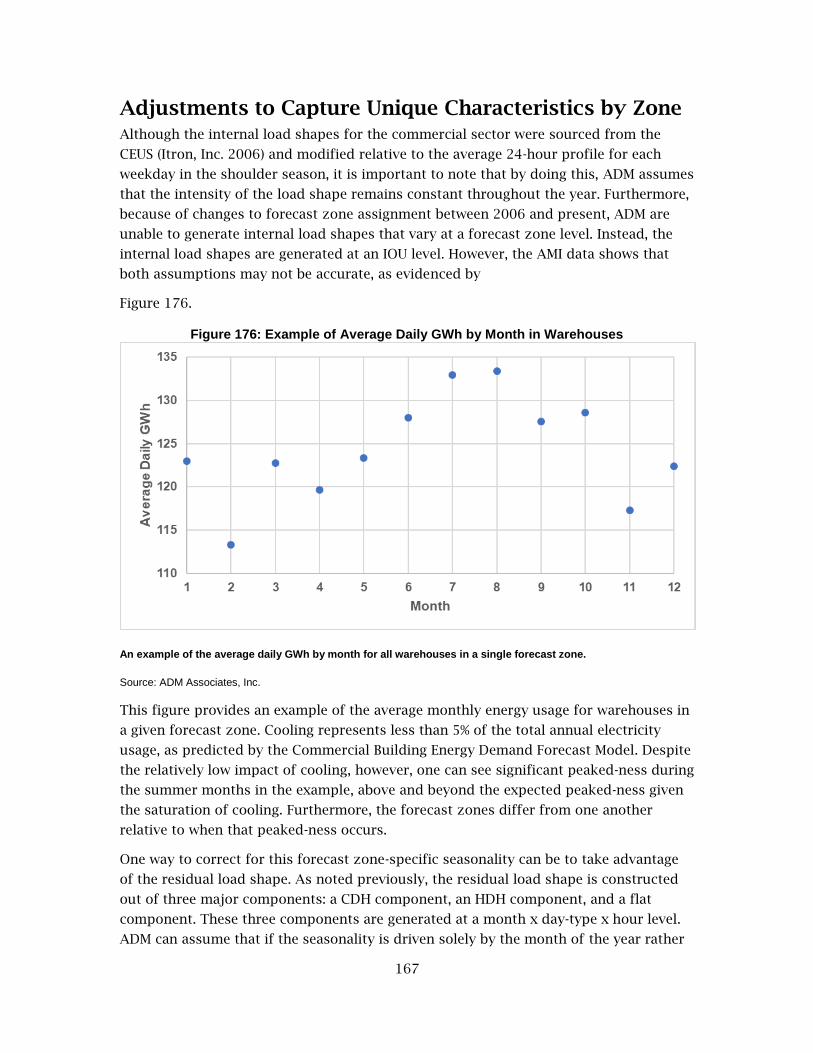
167
Adjustments to Capture Unique Characteristics by Zone Although the internal load shapes for the commercial sector were sourced from the
CEUS (Itron, Inc. 2006) and modified relative to the average 24-hour profile for each
weekday in the shoulder season, it is important to note that by doing this, ADM assumes
that the intensity of the load shape remains constant throughout the year. Furthermore,
because of changes to forecast zone assignment between 2006 and present, ADM are
unable to generate internal load shapes that vary at a forecast zone level. Instead, the
internal load shapes are generated at an IOU level. However, the AMI data shows that
both assumptions may not be accurate, as evidenced by
Figure 176.
Figure 176: Example of Average Daily GWh by Month in Warehouses
An example of the average daily GWh by month for all warehouses in a single forecast zone.
Source: ADM Associates, Inc.
This figure provides an example of the average monthly energy usage for warehouses in
a given forecast zone. Cooling represents less than 5% of the total annual electricity
usage, as predicted by the Commercial Building Energy Demand Forecast Model. Despite
the relatively low impact of cooling, however, one can see significant peaked-ness during
the summer months in the example, above and beyond the expected peaked-ness given
the saturation of cooling. Furthermore, the forecast zones differ from one another
relative to when that peaked-ness occurs.
One way to correct for this forecast zone-specific seasonality can be to take advantage
of the residual load shape. As noted previously, the residual load shape is constructed
out of three major components: a CDH component, an HDH component, and a flat
component. These three components are generated at a month x day-type x hour level.
ADM can assume that if the seasonality is driven solely by the month of the year rather

168
than explicitly by weather, the flat component of the residual load shape should
represent the difference between the modeled non-HVAC components and the true non-
HVAC load.
Using a method like the method used to adjust HVAC load shapes for schools and
colleges on page 131, ADM created scalars to modify the non-HVAC load shapes for all
building types for the years 2014, 2015, and 2016. ADM first began by reconstituting
only the flat component of the residual load shape for each building for each forecast
zone and scaling the load to the appropriate GWh value. Similarly, ADM generated 8,760
load shapes for the non-HVAC loads using the end-use load shapes modeled in
previously in this chapter. These load shapes were then scaled according to the 2014,
2015, and 2016 GWh specified in the Commercial Building Energy Demand Forecast
Model. ADM then aggregated the profiles into two consolidated profiles: the modeled
non-HVAC load shape, which is the aggregation of all non-HVAC loads; and the modeled
profile with flat residual, which aggregated all non-HVAC loads and the modeled flat
component of the residual.
Theoretically, the modeled profile with flat residual should represent the corrected
model of all non-HVAC load shapes at an 8,760 resolution for each of the three base
years. However, there is a margin of error associated with each observation in the 8,760-
load shape. If one assumes that this error is distributed randomly across the 8,760
profile, the margin of error for a single point estimation should reduce as data is
aggregated to higher resolutions. Thus, while error may be persistent at an hourly
resolution, that error should begin to cancel itself out as one moves to looking at data
on a daily level, etc. Furthermore, although ADM could manipulate the non-HVAC load
shapes relative to the 8,760 baseline-subtracted profile, ADM cannot know the
relationship in the 8,760 baseline-subtracted profile and the underlying end-uses and
modifying the modeled end-uses may result in inappropriate changes to the load
shapes.
As a compromise, ADM created scalars that changed the intensity of the internal load
shapes as a function of either month or month by weekday. The goal, ultimately, was to
create a series of scalars to transform the total monthly energy use modeled via the
coefficients to consistently predict total monthly energy usage that was in line with the
version of the load shape that had the flat-residual applied. To accomplish this, ADM
created a monthly and a month x weekday scalar by aggregating the total energy for the
flat-residual applied and unapplied profile at either the monthly or month x weekday
level and dividing the flat-residual applied value by the unapplied value.
ADM then determined which set of scalars would be the most appropriate for each
forecast zone and building type: un-scaled, scaled by month, or scaled by month and
weekday. ADM did this by comparing the NRMSE before and after the application of
each scalar types and selecting the scalar values which provided the greatest reduction
in model error. ADM then modified and stored the coefficients for each non-HVAC load
shape by applying the appropriate scalar for each month or each month x weekday.

169
Figure 177 through
Figure 185 provide examples of Warehouses in a given forecast zone with and without
scalar adjustment.
Figure 177: Comparison of Monthly Energy Usage With and Without Scalar Adjustments
A comparison of the monthly energy usage at the whole building level with and without application of the month
x day scalars but prior to application of the residual load shape.
Source: ADM Associates, Inc.
Figure 178: Average Daily Weekday Profile With and Without Scalar Adjustments in Winter
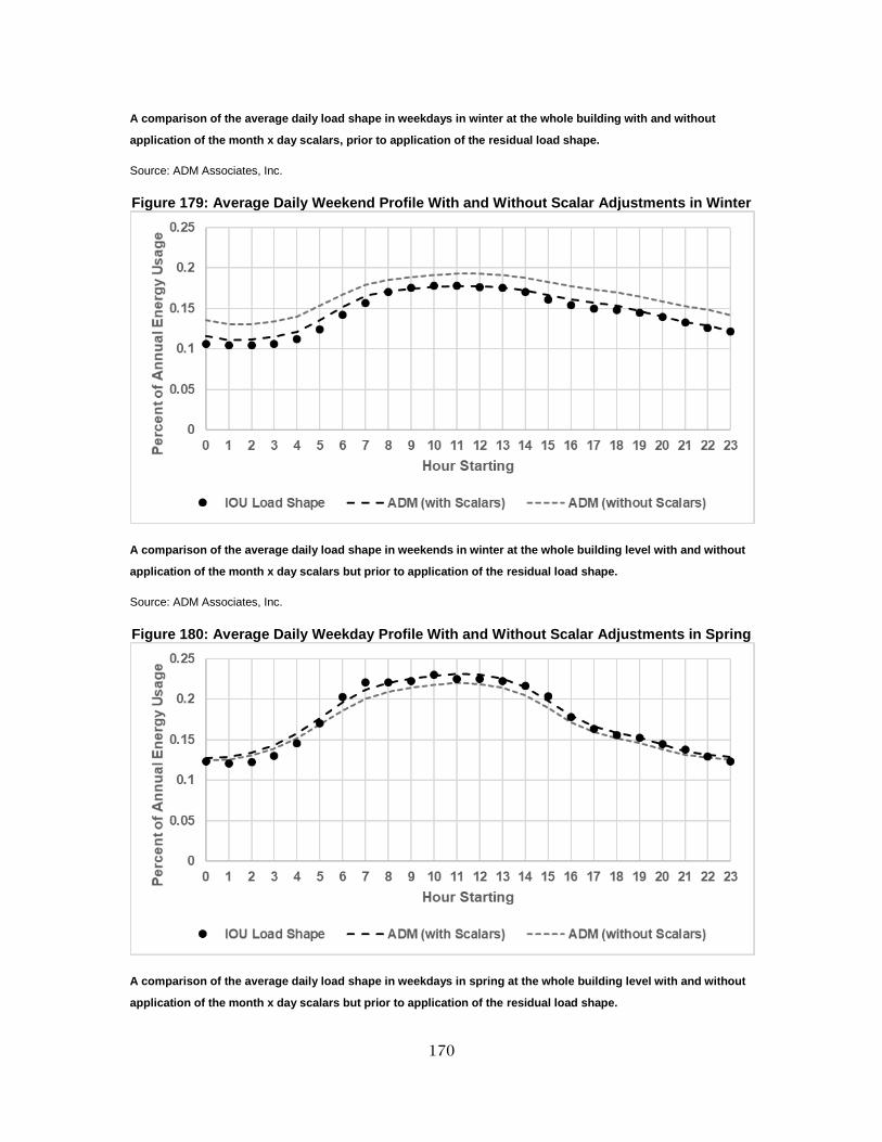
170
A comparison of the average daily load shape in weekdays in winter at the whole building with and without
application of the month x day scalars, prior to application of the residual load shape.
Source: ADM Associates, Inc.
Figure 179: Average Daily Weekend Profile With and Without Scalar Adjustments in Winter
A comparison of the average daily load shape in weekends in winter at the whole building level with and without
application of the month x day scalars but prior to application of the residual load shape.
Source: ADM Associates, Inc.
Figure 180: Average Daily Weekday Profile With and Without Scalar Adjustments in Spring
A comparison of the average daily load shape in weekdays in spring at the whole building level with and without
application of the month x day scalars but prior to application of the residual load shape.

171
Source: ADM Associates, Inc.

172
Figure 181: Average Daily Weekend Profile With and Without Scalar Adjustments in Spring
A comparison of the average daily load shape in weekends in spring at the whole building level with and without
application of the month x day scalars but prior to application of the residual load shape.
Source: ADM Associates, Inc.
Figure 182: Average Daily Weekday Profile With and Without Scalar Adjustments in Summer
A comparison of the average daily load shape in weekdays in summer at the whole building level with and
without application of the month x day scalars but prior to application of the residual load shape.
Source: ADM Associates, Inc.
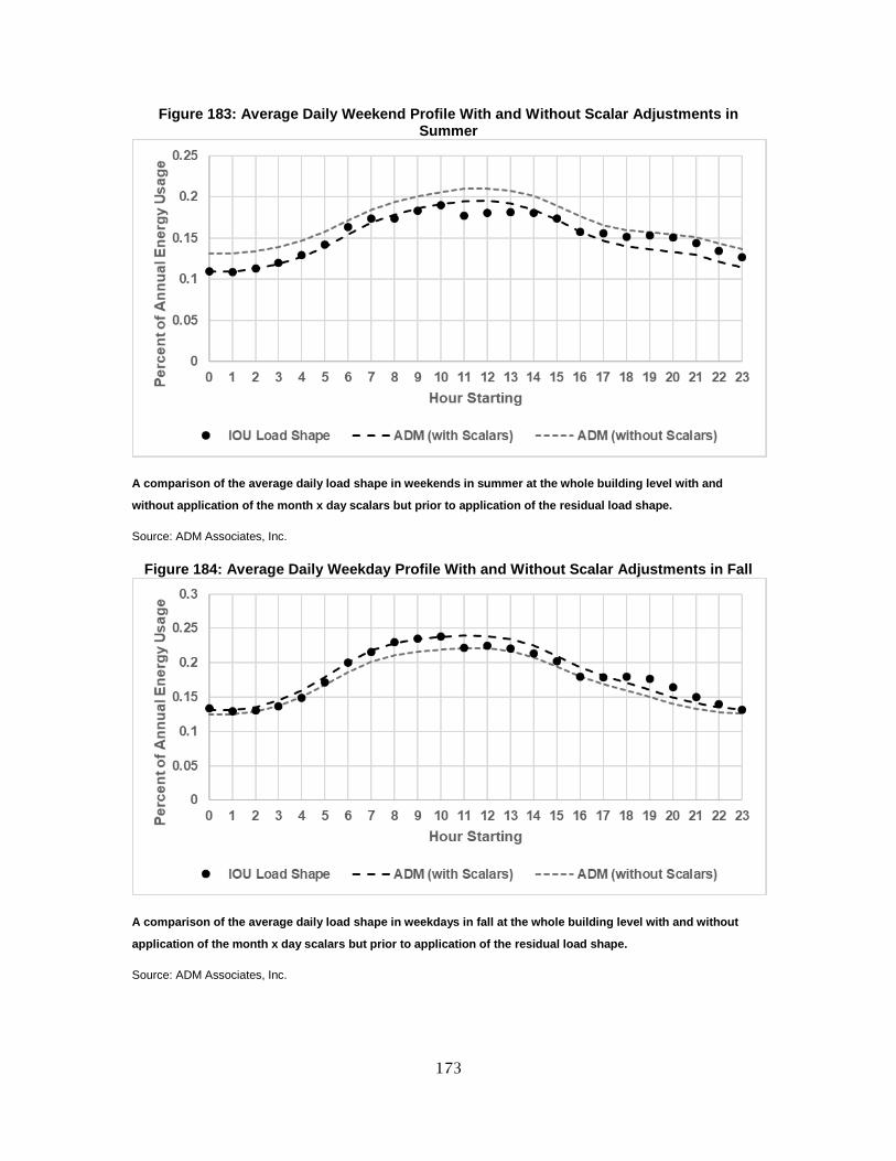
173
Figure 183: Average Daily Weekend Profile With and Without Scalar Adjustments in Summer
A comparison of the average daily load shape in weekends in summer at the whole building level with and
without application of the month x day scalars but prior to application of the residual load shape.
Source: ADM Associates, Inc.
Figure 184: Average Daily Weekday Profile With and Without Scalar Adjustments in Fall
A comparison of the average daily load shape in weekdays in fall at the whole building level with and without
application of the month x day scalars but prior to application of the residual load shape.
Source: ADM Associates, Inc.

174
Figure 185: Average Daily Weekend Profile With and Without Scalar Adjustments in Fall
A comparison of the average daily load shape in weekends in fall at the whole building level with and without
application of the month x day scalars but prior to application of the residual load shape.
Source: ADM Associates, Inc.

175
CHAPTER 4: Base Load Shapes: Agricultural Sector
Unlike the commercial and residential sectors, the Energy Commission’s agricultural
load shapes are not currently generated at the end-use level. Rather, load shapes are
currently isolated to the facility-type only. Energy demand in the agriculture sector
tends to be process-driven, i.e., the load shape for irrigation is primarily driven by the
underlying process and thus most end-uses are also tied to that essential load shape.
There are four facility types represented in the agricultural sector:
Crops
Irrigation
Livestock
Water Supply
ADM’s primary goal for the agricultural sector was to use the AMI data submitted by the
three California IOUs to create a set of coefficients which accurately reflect the typical
load shape for each facility type in each forecast zone and can be used to generate an
8,760-hour load shape for any given year. The remainder of this chapter will describe
the methodology for generating said coefficients.
Regression Modeling To generate sets of coefficients that represent every facility type for every forecast zone,
ADM relied on a regression-based algorithm based on a linear CDH regression model.
Initial considerations were made to determine whether a compression of the data to a
simple 12-month x 24-hour x 8-day matrix would be sufficient for modeling non-
commercial/non-residential sectors. However, visual inspection of the monthly load
shapes shows some variability over a calendar year.

176
Figure 186 illustrates this seasonality, with highest energy use during the summer
months and lower energy use in the winter and shoulder seasons.

177
Figure 186: Example of Monthly Energy Use in the Agricultural Sector
Example of monthly energy use in an Industrial facility-type as taken from across an agricultural facility-type in a
single forecast zone in the 2015 base year.
Source: ADM Associates, Inc.
Because of the seasonal nature of energy use, ADM elected to include a temperature-
based term in the regression equation. Although it is unlikely that the increase in energy
usage during the summer is tied specifically to HVAC, CDH can be used to approximate
variables that are collinear to weather, such as length of day, seasonal production, etc.
ADM opted to use a CDH term rather than an hourly temperature value to mitigate
potential sensitivity as temperature values reach extreme hot or extreme cold values.
Using a CDH variable ensures that as the temperature dips towards negative values, the
term associated with the weather variable cannot become negative.
In addition to the apparent seasonality present in the AMI data, ADM also noted
significant load growth in the AMI data. There is a significant linear relationship
between monthly energy usage and the number of months since the origin point (in this
case, the origin being January of 2015). Therefore, ADM included a “day of year” term
(with 1 representing January 1st) in the regression equation to include a term to capture
the observed linear growth. Although ADM assumed that linear growth will continue to
be present going forward, should someone want to exclude linear growth from a
generated load shape, modeling the effect as part of the regression allows one to do so.
In addition to the main effects described above, ADM also expected the load to vary
relative to weekday type (Sunday-Saturday and observed holidays) and hour of day.
Furthermore, although scheduled loads should theoretically shift in accordance with
daylight savings time, in real-world scenarios, some loads tend to shift relative to
daylight savings time, while other loads end up remaining constant. Thus, ADM also
considered whether an observation fell into PST or PDT an additional main effect for the

178
models. Although the temporal main effects described in this paragraph could be
modeled in a consolidated regression with appropriate interactive terms, ADM opted to
segment the data set by the three temporal criteria (PST/PDT, weekday, and hour). This
yields mathematically identical results while evades computational resource constraints.
After segmenting the data, each segment of data was then run through the following
regression model:
𝑦 = 𝛽0 + 𝛽1 ∙ 𝐶𝐷𝐻 + 𝛽2 ∙ 𝐷𝑎𝑦 𝑜𝑓 𝑌𝑒𝑎𝑟 + 𝜀
Where:
𝑦 is the predicted kW of the building
𝛽0 is the intercept
𝛽1 is the CDH weight
𝛽2 is the linear growth term relative of the day of year (1-365 or 366)
𝜀 is the error term.
The model was run for each data segment and the regression coefficients recorded for
use in the load shape generator.
To select an appropriate CDH base term, ADM iterated through five potential CDH base
values (50 degrees Fahrenheit, 55 degrees Fahrenheit, 60 degrees Fahrenheit, 65 degrees
Fahrenheit, and 70 degrees Fahrenheit) to determine which value provided the lowest
amount of model error, as represented through NRMSE.7
Data Sources The following section provides a list of the data sources used to generate the
agricultural load shapes. In addition to listing the data source, a brief description of the
data source and any data preparation activities are provided.
AMI Data
As part of this project, a data request was submitted to the IOUs requesting data for all
non-residential sectors from the years 2014, 2015, and 2016. In response to this data
request, the IOUs provided averaged hourly data by building sub-type and either usage
level (PG&E and SDG&E segmented data by high, medium, and low users) or rate class
(SCE).
Prior to using the interval meter data, ADM first pre-treated all data. This pre-treatment
consisted of standardizing the nomenclature of all files and merging the dataset with
climate-zone specific hourly historical weather data obtained from the Energy
Commission. Hourly timestamps were standardized to units of PST for the entire year
7 The equation for calculating NRMSE is previously defined in the “Post Calibration Modeling” section of the Commercial chapter, beginning on page 118.
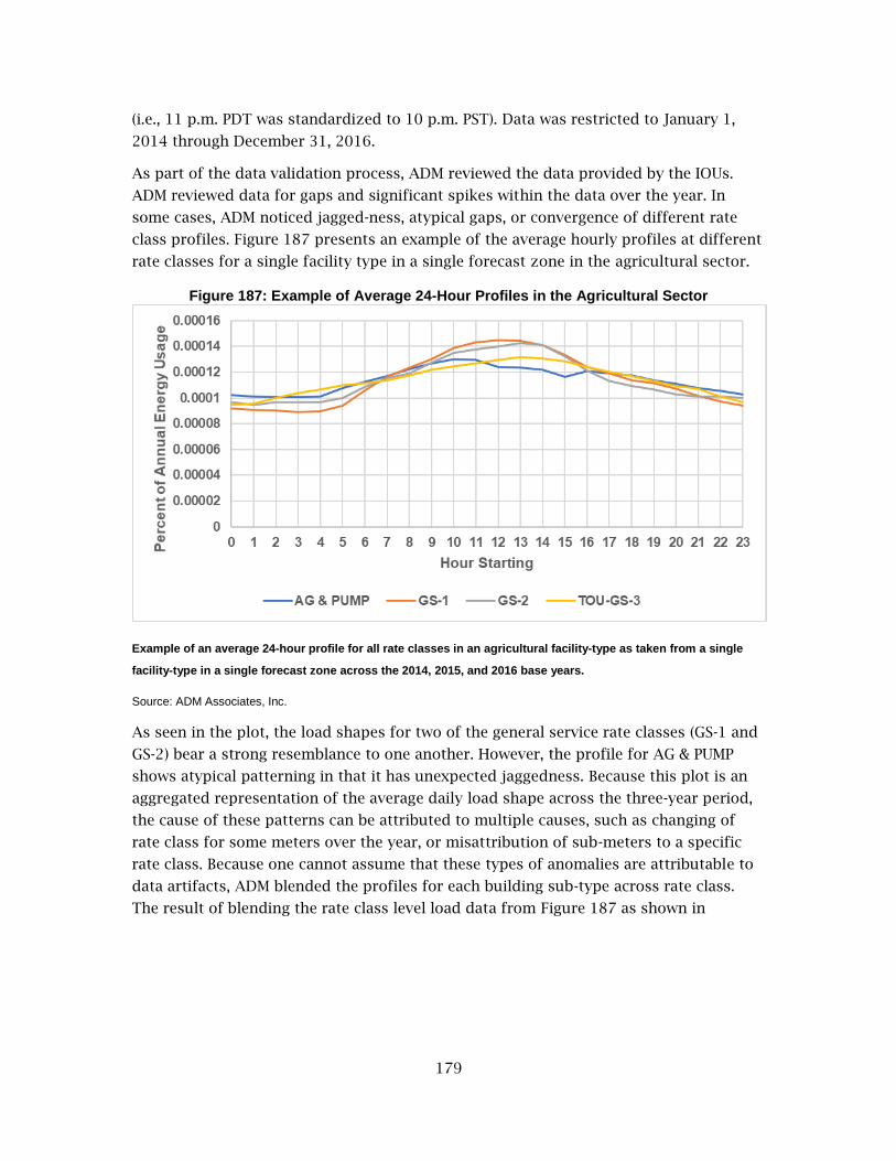
179
(i.e., 11 p.m. PDT was standardized to 10 p.m. PST). Data was restricted to January 1,
2014 through December 31, 2016.
As part of the data validation process, ADM reviewed the data provided by the IOUs.
ADM reviewed data for gaps and significant spikes within the data over the year. In
some cases, ADM noticed jagged-ness, atypical gaps, or convergence of different rate
class profiles. Figure 187 presents an example of the average hourly profiles at different
rate classes for a single facility type in a single forecast zone in the agricultural sector.
Figure 187: Example of Average 24-Hour Profiles in the Agricultural Sector
Example of an average 24-hour profile for all rate classes in an agricultural facility-type as taken from a single
facility-type in a single forecast zone across the 2014, 2015, and 2016 base years.
Source: ADM Associates, Inc.
As seen in the plot, the load shapes for two of the general service rate classes (GS-1 and
GS-2) bear a strong resemblance to one another. However, the profile for AG & PUMP
shows atypical patterning in that it has unexpected jaggedness. Because this plot is an
aggregated representation of the average daily load shape across the three-year period,
the cause of these patterns can be attributed to multiple causes, such as changing of
rate class for some meters over the year, or misattribution of sub-meters to a specific
rate class. Because one cannot assume that these types of anomalies are attributable to
data artifacts, ADM blended the profiles for each building sub-type across rate class.
The result of blending the rate class level load data from Figure 187 as shown in

180
Figure 188: .
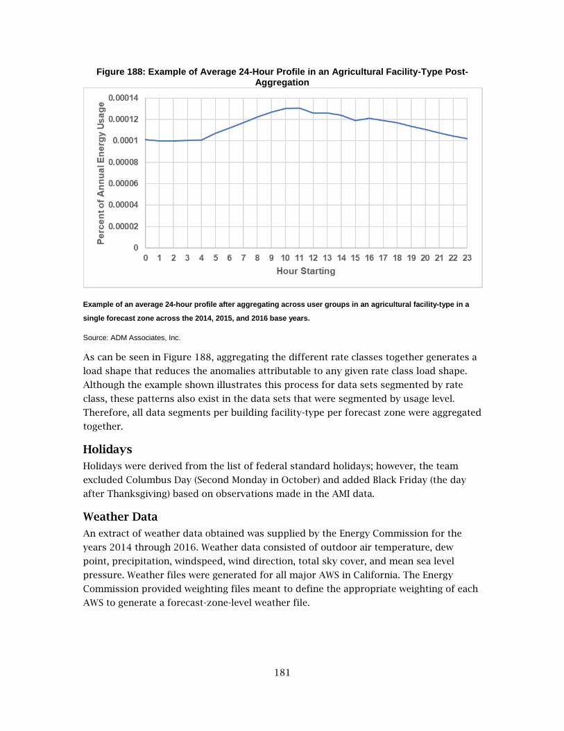
181
Figure 188: Example of Average 24-Hour Profile in an Agricultural Facility-Type Post-Aggregation
Example of an average 24-hour profile after aggregating across user groups in an agricultural facility-type in a
single forecast zone across the 2014, 2015, and 2016 base years.
Source: ADM Associates, Inc.
As can be seen in Figure 188, aggregating the different rate classes together generates a
load shape that reduces the anomalies attributable to any given rate class load shape.
Although the example shown illustrates this process for data sets segmented by rate
class, these patterns also exist in the data sets that were segmented by usage level.
Therefore, all data segments per building facility-type per forecast zone were aggregated
together.
Holidays
Holidays were derived from the list of federal standard holidays; however, the team
excluded Columbus Day (Second Monday in October) and added Black Friday (the day
after Thanksgiving) based on observations made in the AMI data.
Weather Data
An extract of weather data obtained was supplied by the Energy Commission for the
years 2014 through 2016. Weather data consisted of outdoor air temperature, dew
point, precipitation, windspeed, wind direction, total sky cover, and mean sea level
pressure. Weather files were generated for all major AWS in California. The Energy
Commission provided weighting files meant to define the appropriate weighting of each
AWS to generate a forecast-zone-level weather file.

182
CHAPTER 5: Base Load Shapes: Industrial Sector
As with the agricultural sector, the Energy Commission’s industrial load shapes are not
currently generated at the end-use level. Rather, load shapes are currently isolated to
the facility-type only. Energy demand in the industrial sector tends to be process-driven,
i.e., the load shape for primary metals is primarily driven by the underlying fabrication
of primary metals and thus most end-uses are also tied to that essential load shape. To
reduce the overall number of load shapes, ADM mapped the 25 NAICS-based business
types from the forecast model to 15 facility types represented as shown in Table 5. This
mapping is accomplished with data preparation scripts that take the outputs of
individual forecast models (bypassing the Summary Model) and develop inputs for
HELM 2.0. The table can also be incorporated into the Summary Model to facilitate input
to HELM 2.0.
Table 5 – Mapping of 25 NAICS-based industrial classifications to 15 building types.
NAICS ADM Building
311x, 312 Consumable Goods
3113, 3114 Consumable Goods
313 Textiles and Apparel
314 Textiles and Apparel
315, 316 Textiles and Apparel
1133, 321 Logging and Derivatives
322x Logging and Derivatives
3221 Logging and Derivatives
323 Logging and Derivatives
324 Petroleum
325 Chemicals
326 Chemicals
327x Construction Materials
3272 Construction Materials
3273 Construction Materials
331 Primary Metals
332 Fabricated Metal Products
333 Machinery
334x Computers, Electronics
3344 Computers, Electronics
335 Lighting And Appliances
336 Transportation Equipment
337 Furniture
339 Nonelectrical durable goods
511 Publishing Industries
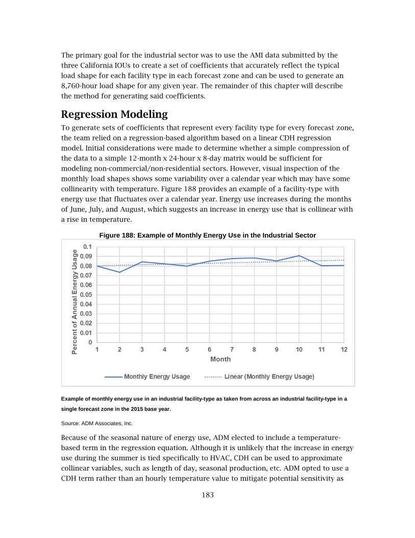
183
The primary goal for the industrial sector was to use the AMI data submitted by the
three California IOUs to create a set of coefficients that accurately reflect the typical
load shape for each facility type in each forecast zone and can be used to generate an
8,760-hour load shape for any given year. The remainder of this chapter will describe
the method for generating said coefficients.
Regression Modeling To generate sets of coefficients that represent every facility type for every forecast zone,
the team relied on a regression-based algorithm based on a linear CDH regression
model. Initial considerations were made to determine whether a simple compression of
the data to a simple 12-month x 24-hour x 8-day matrix would be sufficient for
modeling non-commercial/non-residential sectors. However, visual inspection of the
monthly load shapes shows some variability over a calendar year which may have some
collinearity with temperature. Figure 188 provides an example of a facility-type with
energy use that fluctuates over a calendar year. Energy use increases during the months
of June, July, and August, which suggests an increase in energy use that is collinear with
a rise in temperature.
Figure 188: Example of Monthly Energy Use in the Industrial Sector
Example of monthly energy use in an industrial facility-type as taken from across an industrial facility-type in a
single forecast zone in the 2015 base year.
Source: ADM Associates, Inc.
Because of the seasonal nature of energy use, ADM elected to include a temperature-
based term in the regression equation. Although it is unlikely that the increase in energy
use during the summer is tied specifically to HVAC, CDH can be used to approximate
collinear variables, such as length of day, seasonal production, etc. ADM opted to use a
CDH term rather than an hourly temperature value to mitigate potential sensitivity as

184
temperature values reach extreme hot or extreme cold values. Using a CDH variable
ensures that as the temperature dips towards negative values, the term associated with
the weather variable cannot become negative.
ADM also noted significant load growth in the AMI data. As can be seen in Figure 188,
there is a significant linear relationship between monthly energy usage and the number
of months since the origin point (in this case, the origin being January of 2015).
Therefore, ADM included a “day of year” term (with 1 representing January 1st) in the
regression equation to include a term to capture the observed linear growth. Although
ADM assumed that linear growth will continue to be present going forward, should
someone want to exclude linear growth from a generated load shape, modeling the
effect as part of the regression allows one to do so.
In addition to linear load growth and temperature-correlated factors, ADM also reviewed
the impact of economic growth or decline on the resulting load shape. Because
production in the industrial sector is explicitly tied to economic factors, ADM felt that
changes in the economy could predict changes in the load shape for one year compared
to another. Therefore, ADM included historical economic values as an independent
variable in the model.
In addition to the main effects described above, ADM also expected the load to vary
relative to weekday type (Sunday-Saturday and observed holidays) and hour of day.
Furthermore, although scheduled loads should theoretically shift in accordance with
daylight savings time, in real-world scenarios, some loads tend to shift relative to
daylight savings time, while other loads end up remaining constant. Thus, ADM also
considered whether an observation fell into the daylight savings time period an
additional main effect for the models. Although the temporal main effects described in
this paragraph could be modeled in a consolidated regression with appropriate
interactive terms, ADM opted to segment the data set by the three temporal criteria
(PDT/PST, weekday, and hour). This yields mathematically identical results while evades
computational resource constraints.
After segmenting the data, each segment of data was then run through the following
regression model:
𝑦 = 𝛽0 + 𝛽1 ∙ 𝐶𝐷𝐻 + 𝛽2 ∙ 𝐷𝑎𝑦 𝑜𝑓 𝑌𝑒𝑎𝑟 + 𝛽3 ∙ 𝐸𝑐𝑜𝑛𝑜𝑚𝑖𝑐 𝑃𝑟𝑒𝑑𝑖𝑐𝑡𝑜𝑟 + 𝜀
Where:
𝑦 is the predicted normalized load of the building
𝛽0 is the intercept
𝛽1 is the CDH weight
𝛽2 is the linear growth term relative of the day of year (1-365 or 366)
𝛽3 is the weight of the economic predictor
𝜀 is the error term

185
The above model was run for each data segment and the regression coefficients
recorded for use in the base year load shape generator.
To select an appropriate CDH base term, the team iterated through five potential CDH
base values (50 degrees Fahrenheit, 55 degrees Fahrenheit, 60 degrees Fahrenheit, 65
degrees Fahrenheit, and 70 degrees Fahrenheit) to determine which value provided the
lowest amount of model error, as represented through NRMSE.8
Data Sources The following section provides a list of the data sources used to generate ADM's
industrial load shapes. In addition to listing the data source, a brief description of the
data source and any data preparation activities are provided.
AMI Data
As part of this project, a data request was submitted to the three California IOUs
requesting data for all non-residential sectors from the years 2014, 2015, and 2016. In
response to this data request, the three IOUs provided averaged hourly data by building
sub-type and either usage level (PG&E and SDG&E segmented data by high, medium, and
low users) or rate class (SCE).
Prior to using the interval meter data, ADM first pre-treated all data. This pre-treatment
consisted of standardizing the nomenclature of all files and merging the dataset with
climate-zone specific hourly historical weather data obtained from the Energy
Commission. Hourly timestamps were standardized to units of PST for the entire year
(i.e., 11 p.m. PDT was standardized to 10 p.m. PST). Data was restricted to January 1,
2014 through December 31, 2016.
As part of the data validation process, ADM reviewed the data provided by the IOUs.
ADM data for gaps and significant spikes within the data over the year. The plot in
Figure 189 depicts average daily load shapes obtained across all buildings of a given
facility-type in a single forecast zone at different use levels.
8 The equation for calculating NRMSE is previously defined in the “Post Calibration Modeling” section of the Commercial chapter, beginning on page 118.

186
Figure 189: Example of Average 24-Hour Profiles for a Single Facility Type Across User Groups
Example of an average 24-hour profile for large, medium, and small users in an industrial facility-type as taken
from all building types of a single facility-type in a single forecast zone across the 2014, 2015, and 2016 base
years.
Source: ADM Associates, Inc.
In general, anomalies were not as pervasive in the data sets for the industrial sector as
compared to the data sets obtained for the commercial or agricultural sector. However,
for the purpose of maintaining consistency with the data preparation in other sectors,
the team blended the profiles for each facility-type across rate class or usage level. The
result of blending the rate class level load data from

187
Figure 189 as shown

188
Figure 190.

189
Figure 190: Example of Average 24-Hour Profiles Post-Aggregation
Example of an average 24-hour profile after aggregating across user groups in an industrial facility-type as taken
from all building types of a single facility-type in a single forecast zone across the 2014, 2015, and 2016 base
years.
Source: ADM Associates, Inc.
Economic Forecast Data
An extract of historical and forecasted economic data obtained from Moody’s Analytics,
Inc. was supplied by the Energy Commission for the years 2014 through 2028 at a
quarterly resolution by NAICS category and forecast zone. The economic data provided
for the industrial sector were GSP values in units of current-day millions of dollars.
Holidays
Holidays were derived from the list of federal standard holidays; however, ADM
excluded Columbus Day (Second Monday in October) and added Black Friday (the day
after Thanksgiving) based on observations made in the AMI data. Additionally, AMI data
was reviewed for periods of low energy use to identify potential “holiday” periods. For
each facility type in each forecast zone, the lowest 10% of days per year were identified.
Dates that appeared consistent for more than 50% of all buildings were hallmarked as
potential holidays and reviewed for consistency and clear pattern across the three base
years prior to being designated as “holidays” in the industrial sector. The following
dates were identified as additional Holidays:
The first calendar week of December (which includes the first partial week of
January)
Easter Sunday
Last two calendar weeks of December (which includes the last full week and last
partial week of December)

190
Weather Data
An extract of weather data was supplied by the Energy Commission for the years 2014
through 2016. Weather data consisted of outdoor air temperature, dew point,
precipitation, windspeed, wind direction, total sky cover, and mean sea level pressure.
Weather files were generated for all major AWS in California. The Energy Commission
provided weighting files meant to define the appropriate weighting of each AWS to
generate a forecast-zone-level weather file.

191
CHAPTER 6: Base Load Shapes: Mining and Extraction
As with the agricultural and industrial sector, the Energy Commission’s mining and
extraction load shapes are not currently generated at the end-use level. Rather, load
shapes are currently isolated to the facility-type only. Energy demand in the sector tends
to be process-driven, i.e., the load shape for mining is primarily driven by mining and
thus most end-uses are also tied to that essential load shape. There are three types
represented in the mining and extraction sector:
Mining (NAICS 212)
Oil and gas extraction (NAICS 211, 213)
Construction (NAICS 230)
ADM’s primary goal for the mining and extraction sector was to use the AMI data
submitted by the three California IOUs to create a set of coefficients which accurately
reflect the typical load shape for each facility type in each forecast zone and can be
used to generate an 8,760-hour load shape for any given year. The remainder of this
chapter will describe the methodology for generating said coefficients.
Regression Modeling To generate sets of coefficients that represent every facility type for every forecast zone,
the team relied on a regression-based algorithm based on a linear CDH regression
model. Initial considerations were made to determine whether a simple compression of
the data to a simple 12-month x 24-hour x 8-day matrix would be sufficient for
modeling non-commercial/non-residential sectors. However, visual inspection of the
monthly load shapes shows some variability over a calendar year.

192
Figure 191 illustrates this seasonality, with highest energy use during the summer
months and lower energy use in the winter and shoulder seasons.
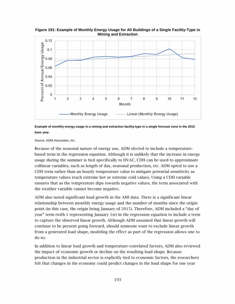
193
Figure 191: Example of Monthly Energy Usage for All Buildings of a Single Facility-Type in Mining and Extraction
Example of monthly energy usage in a mining and extraction facility-type in a single forecast zone in the 2015
base year.
Source: ADM Associates, Inc.
Because of the seasonal nature of energy use, ADM elected to include a temperature-
based term in the regression equation. Although it is unlikely that the increase in energy
usage during the summer is tied specifically to HVAC, CDH can be used to approximate
collinear variables, such as length of day, seasonal production, etc. ADM opted to use a
CDH term rather than an hourly temperature value to mitigate potential sensitivity as
temperature values reach extreme hot or extreme cold values. Using a CDH variable
ensures that as the temperature dips towards negative values, the term associated with
the weather variable cannot become negative.
ADM also noted significant load growth in the AMI data. There is a significant linear
relationship between monthly energy usage and the number of months since the origin
point (in this case, the origin being January of 2015). Therefore, ADM included a “day of
year” term (with 1 representing January 1st) in the regression equation to include a term
to capture the observed linear growth. Although ADM assumed that linear growth will
continue to be present going forward, should someone want to exclude linear growth
from a generated load shape, modeling the effect as part of the regression allows one to
do so.
In addition to linear load growth and temperature-correlated factors, ADM also reviewed
the impact of economic growth or decline on the resulting load shape. Because
production in the industrial sector is explicitly tied to economic factors, the researchers
felt that changes in the economy could predict changes in the load shape for one year

194
compared to another. Therefore, the researchers included historical economic values as
an independent variable in the model.
In addition to the main effects described above, ADM also expected the load to vary
relative to weekday type (Sunday-Saturday and observed holidays) and hour of day.
Furthermore, although scheduled loads should theoretically shift in accordance with
daylight savings time, in real-world scenarios, some loads tend to shift relative to
daylight savings time, while other loads end up remaining constant. Thus, ADM also
considered whether an observation fell into PST or PDT an additional main effect for the
models. Although the temporal main effects described in this paragraph could be
modeled in a consolidated regression with appropriate interactive terms, the
researchers opted to segment the data set by the three temporal criteria (PDT/PST,
weekday, and hour). This yields mathematically identical results while evades
computational resource constraints.
After segmenting the data, each segment of data was then run through the following
regression model:
𝑦 = 𝛽0 + 𝛽1 ∙ 𝐶𝐷𝐻 + 𝛽2 ∙ 𝐷𝑎𝑦 𝑜𝑓 𝑌𝑒𝑎𝑟 + 𝛽3 ∙ 𝐸𝑐𝑜𝑛𝑜𝑚𝑖𝑐 𝑃𝑟𝑒𝑑𝑖𝑐𝑡𝑜𝑟 + 𝜀
Where:
𝑦 is the predicted normalized load of the building
𝛽0 is the intercept
𝛽1 is the CDH weight
𝛽2 is the linear growth term relative of the day of year (1-365 or 366)
𝛽3 is the weight of the economic predictor
𝜀 is the error term
The above model was run for each data segment and the regression coefficients
recorded for use in the base year load shape generator.
To select an appropriate CDH base term, ADM iterated through five potential CDH base
values (50 degrees Fahrenheit, 55 degrees Fahrenheit, 60 degrees Fahrenheit, 65 degrees
Fahrenheit, and 70 degrees Fahrenheit) to determine which value provided the lowest
amount of model error, as represented through NRMSE.9
Data Sources The following section provides a list of the data sources used to generate ADM's load
shapes. In addition to listing the data source, a brief description of the data source and
any data preparation activities are provided.
9 The equation for calculating NRMSE is previously defined in the “Post Calibration Modeling” section of the Commercial chapter, beginning on page 118.

195
AMI Data
As part of this project, a data request was submitted to the three California IOUs
requesting data for all non-residential sectors from the years 2014, 2015, and 2016. In
response to this data request, the three IOUs provided averaged hourly data by building
sub-type and either use level (PG&E and SDG&E segmented data by high, medium, and
low users) or rate class (SCE).
Prior to using the interval meter data, the team first pre-treated all data. This pre-
treatment consisted of standardizing the nomenclature of all files and merging the
dataset with climate-zone specific hourly historical weather data obtained from the
Energy Commission. Hourly timestamps were standardized to units of PST for the entire
year (11 p.m. PDT was standardized to 10 p.m. PST). Data was restricted to January 1,
2014 through December 31, 2016.
As part of ADM's data validation process, ADM reviewed the data provided by the IOUs.
ADM reviewed data for gaps and significant spikes within the data during the year. The
plot in Figure 192 depicts average daily load shapes obtained for an average building in
a single forecast zone of a single mining and Extraction facility-type.
Figure 192: Example of Average 24-Hour Profiles for a Single Mining and Extraction Facility-Type Across Rate Classes
Example of an average 24-hour profile for different rate-classes as taken in a mining and extraction facility-type
as taken from all building types of a single facility-type in a single forecast zone across the 2014, 2015, and 2016
base years.
Source: ADM Associates, Inc.
As seen in the plot, the load shapes are generally inconsistent with one another.
Additionally, the profile for AG & PUMP shows unexpected jaggedness. Because this plot
is an aggregated representation of the average daily load shape across the three-year
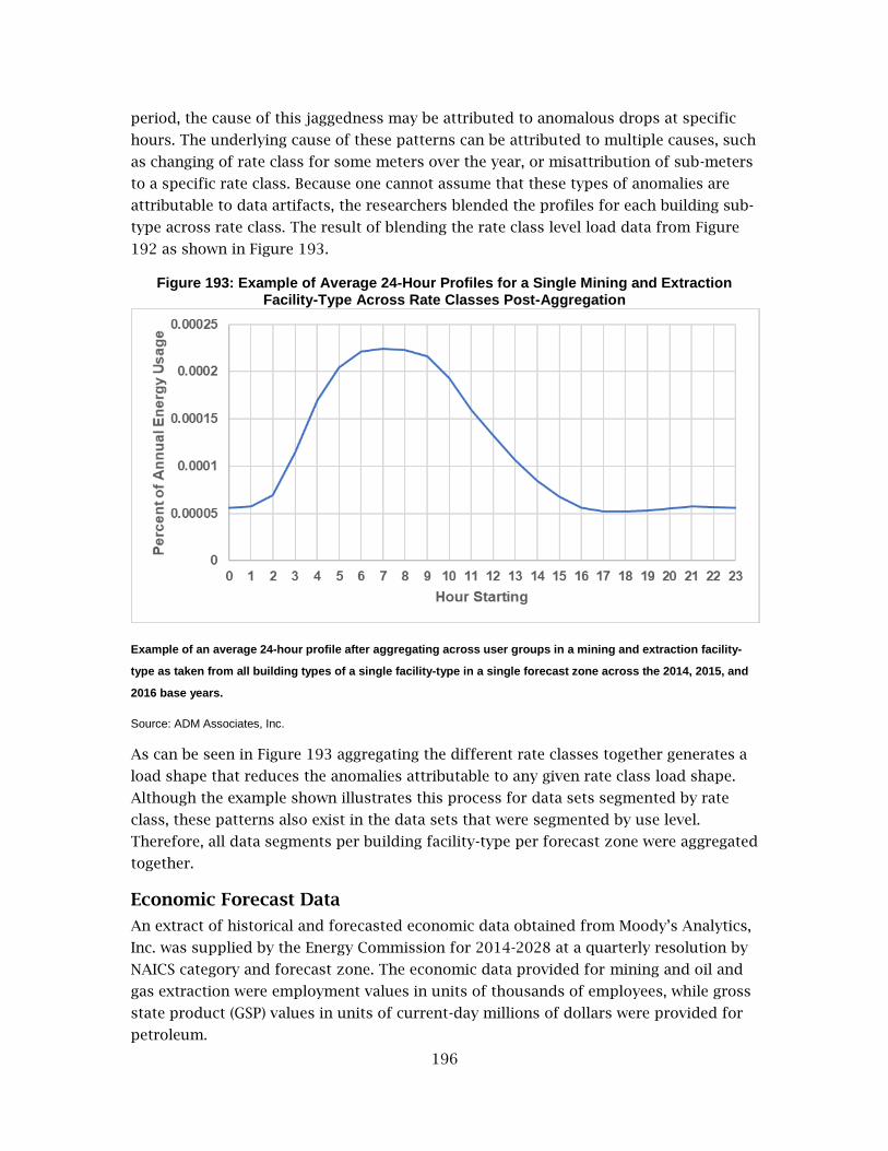
196
period, the cause of this jaggedness may be attributed to anomalous drops at specific
hours. The underlying cause of these patterns can be attributed to multiple causes, such
as changing of rate class for some meters over the year, or misattribution of sub-meters
to a specific rate class. Because one cannot assume that these types of anomalies are
attributable to data artifacts, the researchers blended the profiles for each building sub-
type across rate class. The result of blending the rate class level load data from Figure
192 as shown in Figure 193.
Figure 193: Example of Average 24-Hour Profiles for a Single Mining and Extraction Facility-Type Across Rate Classes Post-Aggregation
Example of an average 24-hour profile after aggregating across user groups in a mining and extraction facility-
type as taken from all building types of a single facility-type in a single forecast zone across the 2014, 2015, and
2016 base years.
Source: ADM Associates, Inc.
As can be seen in Figure 193 aggregating the different rate classes together generates a
load shape that reduces the anomalies attributable to any given rate class load shape.
Although the example shown illustrates this process for data sets segmented by rate
class, these patterns also exist in the data sets that were segmented by use level.
Therefore, all data segments per building facility-type per forecast zone were aggregated
together.
Economic Forecast Data
An extract of historical and forecasted economic data obtained from Moody’s Analytics,
Inc. was supplied by the Energy Commission for 2014-2028 at a quarterly resolution by
NAICS category and forecast zone. The economic data provided for mining and oil and
gas extraction were employment values in units of thousands of employees, while gross
state product (GSP) values in units of current-day millions of dollars were provided for
petroleum.

197
Holidays
Holidays were derived from the list of federal standard holidays; however, the team
excluded Columbus Day (Second Monday in October) and added Black Friday (the day
after Thanksgiving) based on observations made in the AMI data. Additionally, AMI data
was reviewed for periods of low energy use to identify potential “holiday” periods. For
each facility type in each forecast zone, the lowest 10% of days per year were identified.
Dates that appeared consistent for more than 50% of all buildings were hallmarked as
potential holidays and reviewed for consistency and clear pattern across the three base
years prior to being designated as “holidays” in the mining and extraction sector. The
following dates were identified as additional holidays:
Christmas Eve
New Year’s Eve
Weather Data
An extract of weather data obtained from was supplied by the Energy Commission for
the years 2014 through 2016. Weather data consisted of outdoor air temperature, dew
point, precipitation, windspeed, wind direction, total sky cover, and mean sea level
pressure. Weather files were generated for all major AWS in California. The Energy
Commission provided weighting files meant to define the appropriate weighting of each
AWS to generate a forecast-zone-level weather file.

198
CHAPTER 7: Base Load Shapes: TCU Load Shapes
As with the other non-residential and non-commercial sectors, the Energy Commission’s
TCU sector load shapes are not currently generated at the end-use level. Rather, load
shapes are currently isolated to the facility-type only. Energy demand in the TCU sector
tends to be process-driven, specifically the load shape for wireless telecommunications
is primarily driven by wireless telecommunications and thus most end-uses are also tied
to that essential load shape. There are 13 facility-types in the TCU sector:
Air transportation,
Broadcasting,
Ground transportation,
Motor freight,
National security,
Pipelines,
Postal service,
Railroad transportation,
Rental and leasing services,
Utilities,
Waste management,
Water transportation and sightseeing,
Wireless telecommunication.
ADM’s primary goal for the TCU sector was to use the AMI data submitted by the three
California IOUs to create a set of coefficients which accurately reflect the typical load
shape for each facility type in each forecast zone and can be used to generate an 8,760-
hour load shape for any given year. The remainder of this chapter will describe the
methodology for generating said coefficients.
Regression Modeling To generate sets of coefficients that represent every facility type for every forecast zone,
the researchers relied on a regression-based algorithm based on a linear CDH regression
model. Initial considerations were made to determine whether a simple compression of
the data to a simple 12-month x 24-hour x 8-day matrix would be sufficient for
modeling non-commercial/non-residential sectors. However, visual inspection of the
monthly load shapes shows some variability over a calendar year. Figure 194 illustrates
this seasonality, with highest energy use during the summer months and lower energy
use in the winter and shoulder seasons.
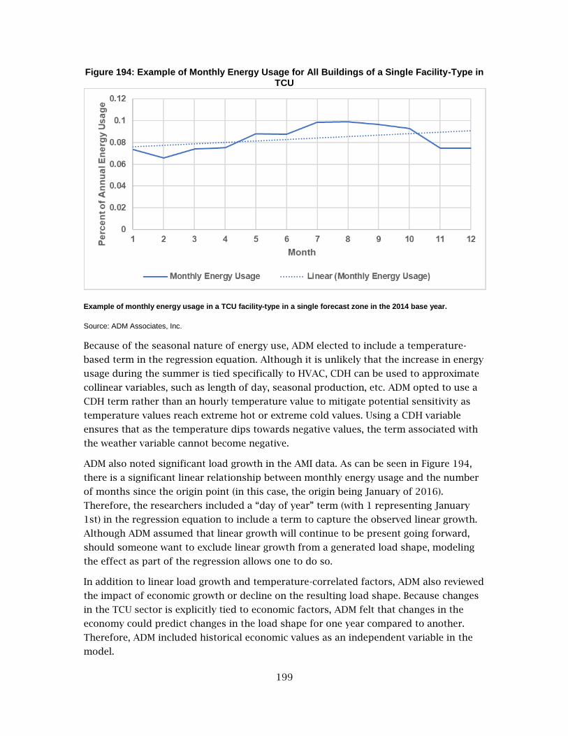
199
Figure 194: Example of Monthly Energy Usage for All Buildings of a Single Facility-Type in TCU
Example of monthly energy usage in a TCU facility-type in a single forecast zone in the 2014 base year.
Source: ADM Associates, Inc.
Because of the seasonal nature of energy use, ADM elected to include a temperature-
based term in the regression equation. Although it is unlikely that the increase in energy
usage during the summer is tied specifically to HVAC, CDH can be used to approximate
collinear variables, such as length of day, seasonal production, etc. ADM opted to use a
CDH term rather than an hourly temperature value to mitigate potential sensitivity as
temperature values reach extreme hot or extreme cold values. Using a CDH variable
ensures that as the temperature dips towards negative values, the term associated with
the weather variable cannot become negative.
ADM also noted significant load growth in the AMI data. As can be seen in Figure 194,
there is a significant linear relationship between monthly energy usage and the number
of months since the origin point (in this case, the origin being January of 2016).
Therefore, the researchers included a “day of year” term (with 1 representing January
1st) in the regression equation to include a term to capture the observed linear growth.
Although ADM assumed that linear growth will continue to be present going forward,
should someone want to exclude linear growth from a generated load shape, modeling
the effect as part of the regression allows one to do so.
In addition to linear load growth and temperature-correlated factors, ADM also reviewed
the impact of economic growth or decline on the resulting load shape. Because changes
in the TCU sector is explicitly tied to economic factors, ADM felt that changes in the
economy could predict changes in the load shape for one year compared to another.
Therefore, ADM included historical economic values as an independent variable in the
model.
200
In addition to the main effects described above, ADM also expected the load to vary
relative to weekday type (Sunday-Saturday and observed holidays) and hour of day.
Furthermore, although scheduled loads should theoretically shift in accordance with
daylight savings time, in real-world scenarios, some loads tend to shift relative to
daylight savings time, while other loads end up remaining constant. Thus, the team also
considered whether an observation fell into PDT or PST an additional main effect for the
models. Although the temporal main effects described in this paragraph could be
modeled in a consolidated regression with appropriate interactive terms, ADM opted to
segment the data set by the three temporal criteria (PDT/PST, weekday, and hour). This
yields mathematically identical results while evades computational resource constraints.
After segmenting the data, each segment of data was then run through the following
regression model:
𝑦 = 𝛽0 + 𝛽1 ∙ 𝐶𝐷𝐻 + 𝛽2 ∙ 𝐷𝑎𝑦 𝑜𝑓 𝑌𝑒𝑎𝑟 + 𝛽3 ∙ 𝐸𝑐𝑜𝑛𝑜𝑚𝑖𝑐 𝑃𝑟𝑒𝑑𝑖𝑐𝑡𝑜𝑟 + 𝜀
Where:
𝑦 is the predicted normalized load of the building
𝛽0 is the intercept
𝛽1 is the CDH weight
𝛽2 is the linear growth term relative of the day of year (1-365 or 366)
𝛽3 is the weight of the economic predictor
𝜀 is the error term
The above model was run for each data segment and the regression coefficients
recorded for use in the base year load shape generator.
To select an appropriate CDH base term, the researchers iterated through five potential
CDH base values (50 degrees Fahrenheit, 55 degrees Fahrenheit, 60 degrees Fahrenheit,
65 degrees Fahrenheit, and 70 degrees Fahrenheit) to determine which value provided
the lowest amount of model error, as represented through NRMSE.10
Data Sources The following section provides a list of the data sources used to generate TCU load
shapes. In addition to listing the data source, a brief description of the data source and
any data preparation activities are provided.
AMI Data
As part of this project, a data request was submitted to the three California IOUs
requesting data for all non-residential sectors from the years 2014, 2015, and 2016. In
response to this data request, the three IOUs provided averaged hourly data by building
10 The equation for calculating NRMSE is previously defined in the “Post Calibration Modeling” section of the Commercial chapter, beginning on page 118.

201
sub-type and either usage level (PG&E and SDG&E segmented data by high, medium, and
low users) or rate class (SCE).
Prior to using the interval meter data, ADM first pre-treated all data. This pre-treatment
consisted of standardizing the nomenclature of all files and merging the dataset with
climate-zone specific hourly historical weather data obtained from the Energy
Commission. Hourly timestamps were standardized to units of PST for the entire year
(i.e., 11 p.m. PDT was standardized to 10 p.m. PST). Data was restricted to the period of
January 1, 2014 through December 31, 2016.
As part of the data validation process, the team reviewed the data provided by the IOUs.
ADM reviewed data for gaps and significant spikes within the data over the year. The
plot in Figure 195 depicts average daily load shapes obtained for a TCU facility-type in a
single forecast zone.
Figure 195: Example of Average 24-Hour Profiles for a Single TCU Facility-Type Across Rate Classes
Example of an average 24-hour profile for different rate-classes as taken in a TCU facility-type as taken from all
building types of a single facility-type in a single forecast zone across the 2014, 2015, and 2016 base years.
Source: ADM Associates, Inc.
As seen in the plot, the load shapes are generally inconsistent with one another,
although anomalies were not as pervasive in the data sets for the TCU sector as
compared to the data sets obtained for the commercial or agricultural sector. However,
to maintain consistency with the data preparation in other sectors, ADM blended the
profiles for each facility-type across rate class or usage level. The result of blending the
rate class level load data from Figure 195 as shown in
Figure 196.
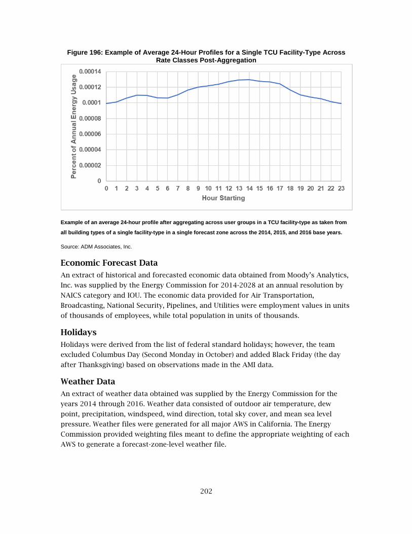
202
Figure 196: Example of Average 24-Hour Profiles for a Single TCU Facility-Type Across Rate Classes Post-Aggregation
Example of an average 24-hour profile after aggregating across user groups in a TCU facility-type as taken from
all building types of a single facility-type in a single forecast zone across the 2014, 2015, and 2016 base years.
Source: ADM Associates, Inc.
Economic Forecast Data
An extract of historical and forecasted economic data obtained from Moody’s Analytics,
Inc. was supplied by the Energy Commission for 2014-2028 at an annual resolution by
NAICS category and IOU. The economic data provided for Air Transportation,
Broadcasting, National Security, Pipelines, and Utilities were employment values in units
of thousands of employees, while total population in units of thousands.
Holidays
Holidays were derived from the list of federal standard holidays; however, the team
excluded Columbus Day (Second Monday in October) and added Black Friday (the day
after Thanksgiving) based on observations made in the AMI data.
Weather Data
An extract of weather data obtained was supplied by the Energy Commission for the
years 2014 through 2016. Weather data consisted of outdoor air temperature, dew
point, precipitation, windspeed, wind direction, total sky cover, and mean sea level
pressure. Weather files were generated for all major AWS in California. The Energy
Commission provided weighting files meant to define the appropriate weighting of each
AWS to generate a forecast-zone-level weather file.

203
CHAPTER 8: Base Load Shapes: Streetlighting
As with the other non-residential and non-commercial sectors, the Energy Commission’s
streetlighting sector load shapes are not currently generated at the end-use level.
Rather, load shapes are currently isolated to holistic “streetlighting” load shapes for
each forecast zone. Unlike the other sectors, streetlighting, which refers primarily to
outdoor lighting fixtures such as street lamps, and traffic signals, remain largely
unmetered as their energy usage is governed by rate tariffs.
Interval meter data provided by the three California IOUs showed reduced, yet
significant usage during daytime, indicating that the metered data available to utilities
are comprised of area lighting as well as lights that are always on, such as traffic lights.
ADM decided to develop an overall streetlighting shape as a mix of two general
components: photocell-controlled streetlighting and always-on traffic signals.
Photocell Load Shape ADM generated a load shape that is consistent with lights controlled by photocells or
astronomical time clocks. One load shape suffices to be representative at the statewide
level, as the key characteristic is that the lights are off from dawn to dusk. Sunrise and
sunset times are readily available on various online websites. ADM found the
Astronomical Data Portal from the United Kingdom Hydrographic Office (2012) to be
particularly useful, and selected Merced, California for its central location and converted
the sundown and sunrise times to lamp run-times. To simulate the effects of photocells
or astronomical time clocks, ADM turned photocells on 15 minutes after sunrise, and 15
minutes before sunset, resulting in 4,152 hours of operation per year.
Traffic Lights Traffic lights tend to have “flat” load shapes. For example, either the red, yellow, or
green traffic light is on at any given time.
Weighting to Represent Nonmetered Streetlighting Based on dimensionality arguments, one would expect streetlighting energy usage to be
orders of magnitude larger than traffic lighting energy usage. To estimate the total
weight of traffic lights, ADM used a survey of street and traffic lighting published by the
League of Oregon Cities (LOC 2010, 13-40). The report lists the number of traffic lights
and street lights in dozens of towns and cities in Oregon. Interestingly, traffic lighting
and street lighting tend to be well represented by linear functions of overall population,
over large population range. On average, traffic lights account for 0.26% of the overall
street and traffic lighting energy use.

204
CHAPTER 9: PV Load Shapes
Method ADM’s approach to modeling PV load shapes included sensitivity studies, data
gathering, performance simulation, and time-averaging of results.
SAM Modeling and Sensitivity Studies ADM started by inspecting load shapes from several typical residential PV systems and
configurations. By comparing results from numerous simulations, ADM quickly
determined that the particular make and model, or even inverter type had negligible
effects on the generation load shapes. The most significant factors were location,
orientation, tilt, and shading of the panels. Shading, however, was only influential in
extreme cases—any amount shading that would qualify for rebates from the CSI did not
result in significant variation of overall output or load shapes. Given the relative
importance of geographical location and orientation, ADM decided to create, for each
forecast zone, four separate load shapes corresponding to panels oriented in the four
cardinal directions. Panel tilt had minor impacts on load shapes, and ADM selected
market-average tilts of 22 for residential installations and 14 for commercial
installations. Although data do not exist to characterize “market average” shading
percentages, ADM applied reasonable estimates based on inspection of satellite
photographs of solar panel installations, and by referencing the CSI eligibility
requirements with respect to shading.
Data Sources The SAM includes libraries of data required for performance simulation, including
weather data and PV system specifics. To characterize market average installation tilts
and fractions of installations in various orientations, ADM used the “Currently
Interconnected Data Set” from the California Distributed Generation Statistics11 website.
The data set includes system and installation specifics from thousands of extant
systems.
Time Averaging of PV Output The SAM can simulate PV generation under various weather conditions. In building
energy simulations, it is customary to use Typical Meteorological Year (TMY) weather
files, which contain actual historic weather data, including heat waves, cold snaps, and
11 Energy Solutions, 2016. California Distributed Generation Statistics. California Public Utilities Commission. https://www.californiadgstats.ca.gov/.

205
other weather events. Average weather, as opposed to typical weather, would lead to
underestimations of peak cooling and heating loads. Application of TMY data might
have unintended consequences, however, in simulations of solar power output. It is not
guaranteed that PV generation and electric demand are synchronized or strongly
correlated. Heat waves occur for complex reasons, which may not be predictably
correlated to PV generation output. For this reason, it is desirable to think of solar
generation in terms of expectation values for given days and hours of the year. For
example, forecasters may want to know, what fraction of the total annual PV generation
output is likely to occur on August 28. Data from any one year may have August 28 as a
particularly cloudy or sunny day, but an average over several years will approximate the
likelihood that August 28 is cloudy. ADM simulated generation using actual weather
data from 2012-2017, as weather data was available for these years at the resolution
needed to run the SAM. All six sets of runs were averaged to create the PV generation
profiles for each forecast zone and sector.

206
CHAPTER 10: EV Charging Load Shapes
Methodology ADM recognized early on that EV charging load shapes are of increasing importance as
the transportation market embarks on historic changes with respect to fuel diversity,
and particularly with electric demand. One challenge associated with forecasting the
time-variable aspect of electric demand in the transportation sector is that most of the
electric demand is yet to come. ADM’s approach was to collect contemporary data on
vehicle charging patterns, while modeling dynamic price response as more customers
switch to grid-integrated rates in the future.
Data Sources The project team attempted to obtain recent and representative data on charging load
shapes.
Vehicle charging session data from ChargePoint
Individually metered residential charging profiles from the Joint IOU Electric
Vehicle Load Research Report
Trending data from bus and shuttle fleets
Energy Commission Staff Report - California Plug-In Electric Vehicle
Infrastructure Projections 2017-2025
Light-Duty Plug-in Electric Vehicle Energy and Emission Calculator from the 2017
IEPR12
Forecast scenarios related to time of use rates offered by IOUs
Conversations with the Energy Commission Transportation Energy Forecasting
Unit staff regarding forecast process for light duty, medium duty, and heavy-
duty vehicles
Single Family Residential Charging Data
ADM obtained a random sample of charging session data from ChargePoint.
ChargePoint is the world’s largest network of EV charging stations, and also provides
chargers for residential use, in single family and multifamily settings. ADM ordered
charging session data from the calendar year 2017 for 500 single family residential
accounts, and 2,000 commercial accounts – 95 of which were installed in multifamily
apartment complexes. The data were anonymized but included important data fields
12 (Yowell, 2018) https://www.energy.ca.gov/sb350/IRPs/documents/Light_Duty_Plug-In_EV_Energ_and_Emission_Calculator.xlsx

207
such as charging session start and end times, total charging energy in kilowatt hours
(kWh), charger maximum capacity, car make and model, battery capacity, and zip code
of charger installation location.
The single family charging data included vehicle make and model, as well as battery
capacity. Given that the typical battery capacity is expected to continue to increase over
the next decade, the team reviewed charging profiles by battery capacity. Figure 197
below shows the typical daily charging profile for cars of various battery capacities. In
the 2017 ChargePoint data, only 62 vehicles had battery capacities of 59 kWh or greater,
and 56 of them were Chevrolet Bolts. Large-battery vehicles tend to start and finish
charging significantly later than other vehicles, which are basically indistinguishable
from each other. ADM has confirmed with ChargePoint that the difference in start time
is not due to a systematic data issue such as one make/model (necessarily, the Bolts)
being reported on Eastern Time rather than Pacific Time. The most likely cause for the
late charging start is that the larger-battery vehicles are typically newer and have
advanced charging menus that enable customers to enter utility rate schedules to
ensure charging starts during off-peak periods.
Figure 197: 2017 Summer Weekday Charging Profile by Battery Capacity
Typical hourly load shapes in summer weekdays for plug-in hybrid vehicles (dashed profile), and battery electric
vehicles with small battery capacities (light grey profile), medium battery capacities, (solid dark grey profile), and
large battery capacities (solid profile with markers). The late charging start for the larger capacity vehicles is
likely due to the fact that the larger battery vehicles are late-model cars with advanced charging menus.
Source: ADM Associates, Inc, data from ChargePoint
0%
2%
4%
6%
8%
10%
12%
14%
16%
1 2 3 4 5 6 7 8 9 10 11 12 13 14 15 16 17 18 19 20 21 22 23 24
Per
cen
t o
f D
ail
y En
ergy
Usa
ge
Residential Charger Profile by Car Battery Capacity
Large (>59kWh) n=62 Medium (24-59 kWh) n=122
Small (<24 kWh) n=185 PHEV n=121

208
Most of the chargers were level two chargers with maximum charging capacities
between 6 kW and 8 kW. Therefore, the total and peak energy demand for a given
charging session was strongly determined by the charging depth, defined here as the
total energy transferred during a charging session. Figure 198 shows hourly charging
demands on summer weekdays for charging sessions of various depths. Deep charges
corresponded, on average, to 37 kWh of energy usage per day. Medium charges averaged
15 kWh. Shallow charges averaged 6 kWh. Most of the excess energy demand for deep
charges, however, occurs during off-peak periods.
Figure 198: 2017 Summer Weekday Charging Demand by Charging Depth
Typical hourly electric demand in summer weekdays for shallow charges (dashed profile), medium charges (dark
solid profile) and deep charges (solid profile with markers).
Source: ADM Associates, Inc, data from ChargePoint
The data in Figure 198 can be deceiving because they portray demands associated with
individual charging sessions. Deep charges require more energy but are likely to be less
frequent, given a fixed overall charging demand in a given geographical area. The grid
experiences the diversified impact of charging, rather than individual loads. To gain the
grid’s perspective, the data in Figure 198 are normalized to percentage of daily energy
usage by hour. Results are shown in
Figure .
0
1
2
3
4
5
6
1 2 3 4 5 6 7 8 9 10 11 12 13 14 15 16 17 18 19 20 21 22 23 24
Ave
rage
Ho
url
y D
em
and
(kW
)
Residential Charging Demand by Charging Depth
Deep (> 25kWh) n=931 Medium (10-25 kWh) n=8583 Shallow (<10kWh) n=8053
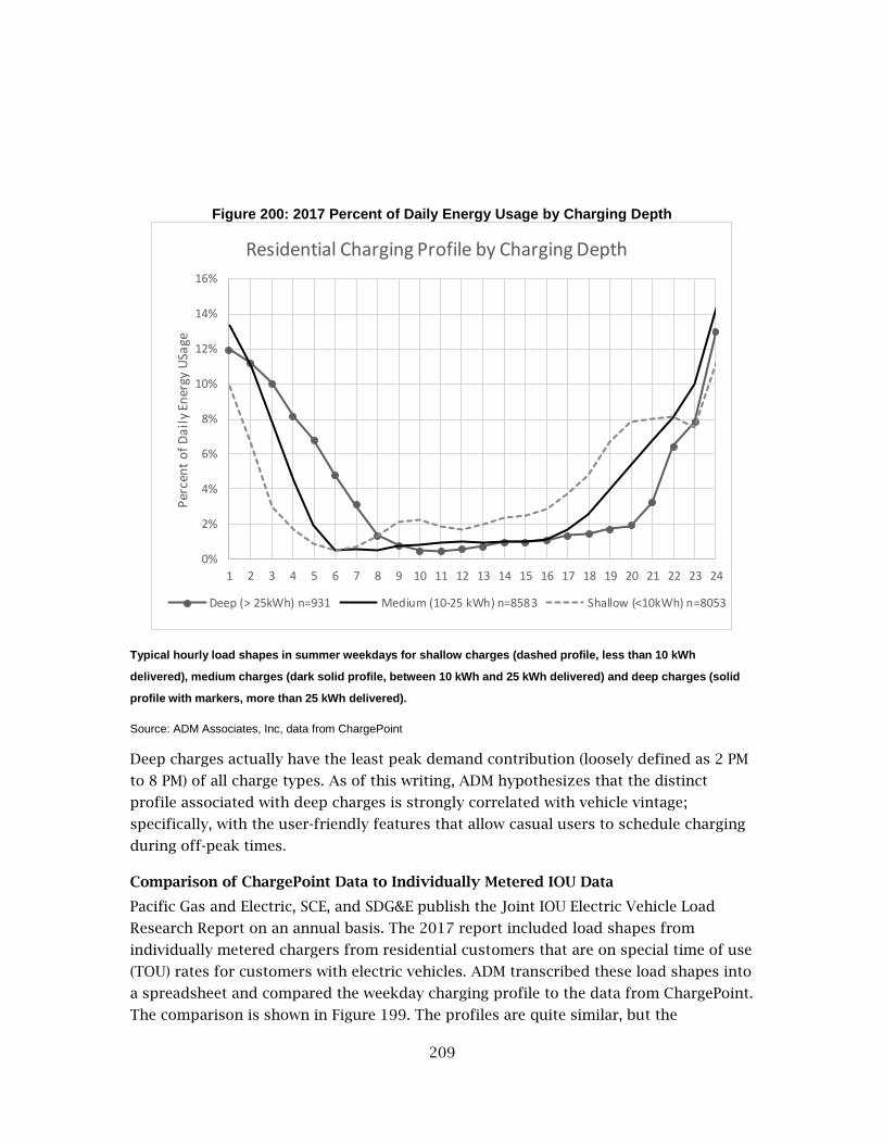
209
Figure 200: 2017 Percent of Daily Energy Usage by Charging Depth
Typical hourly load shapes in summer weekdays for shallow charges (dashed profile, less than 10 kWh
delivered), medium charges (dark solid profile, between 10 kWh and 25 kWh delivered) and deep charges (solid
profile with markers, more than 25 kWh delivered).
Source: ADM Associates, Inc, data from ChargePoint
Deep charges actually have the least peak demand contribution (loosely defined as 2 PM
to 8 PM) of all charge types. As of this writing, ADM hypothesizes that the distinct
profile associated with deep charges is strongly correlated with vehicle vintage;
specifically, with the user-friendly features that allow casual users to schedule charging
during off-peak times.
Comparison of ChargePoint Data to Individually Metered IOU Data
Pacific Gas and Electric, SCE, and SDG&E publish the Joint IOU Electric Vehicle Load
Research Report on an annual basis. The 2017 report included load shapes from
individually metered chargers from residential customers that are on special time of use
(TOU) rates for customers with electric vehicles. ADM transcribed these load shapes into
a spreadsheet and compared the weekday charging profile to the data from ChargePoint.
The comparison is shown in Figure 199. The profiles are quite similar, but the
0%
2%
4%
6%
8%
10%
12%
14%
16%
1 2 3 4 5 6 7 8 9 10 11 12 13 14 15 16 17 18 19 20 21 22 23 24
Per
cen
t o
f D
ail
y En
ergy
USa
ge
Residential Charging Profile by Charging Depth
Deep (> 25kWh) n=931 Medium (10-25 kWh) n=8583 Shallow (<10kWh) n=8053

210
ChargePoint data tends to show demand growth at 4 PM, whereas the IOU data shows
suppressed demand until 8 PM. The likely cause of this difference is that 100% of IOU
customers are on TOU rates, whereas a much smaller fraction of the ChargePoint
customers are on TOU rates. Although the utility rates are not known for the
ChargePoint customers, ADM estimates that 24% of electric IOU customers that were
electric vehicle owners, were on TOU rates in 201713.
Figure 199: 2017 Comparison of Charging Profiles Developed from the Joint IOU Report and ChargePoint Data
Typical hourly load shapes in summer weekdays for single family homes as from the Joint IOU report (solid
profile, averaged over all utilities) and ChargePoint (dashed profile). Note that 100% of customers in the Joint IOU
data set are on time of use rates, whereas the authors estimate that only fewer than 50% of ChargePoint
customers were likely to be on time of use rates in 2017.
Source: ADM Associates, Inc, data from PG&E, SCE, SDG&E, and ChargePoint
Multifamily Residential Charging Data
The ChargePoint data also included session data for 95 chargers in multifamily
apartments. The multifamily data appear to be less concentrated in the off-peak
periods, as shown in Figure 200. ADM does not have additional data to explain the
difference in load shapes, but ADM has excluded the possibility that the type or vintage
of electric vehicles are significantly different between the two housing types. One
13 This quantity is derived in the subsequent section regarding price elasticity.
0%
2%
4%
6%
8%
10%
12%
14%
16%
18%
1 2 3 4 5 6 7 8 9 10 11 12 13 14 15 16 17 18 19 20 21 22 23 24
Perc
ent
of
Dai
ly E
ner
gy U
Sage
Residential Charger Profile by Data Source
IOUs (ChargePoint, 2017) IOUs (Joint IOU Report, 2017)

211
possible explanation is that some of the multifamily chargers may be on commercial
accounts associated with property management rather than individual tenants, and as a
result the price response may be less acute.
Figure 200: 2017 Charging Profiles for Single Family and Multifamily Homes
Typical hourly load shapes in summer weekdays for single family homes (solid profile) and multifamily homes
(dashed profile).
Source: ADM Associates, Inc, data from ChargePoint
Nonresidential Light Duty Vehicle Charging Data
ADM obtained a random sample of non-residential charging session data from
ChargePoint. The data were anonymized, but included a specification of the business
type associated with the charging station. Although all chargers are installed in the
commercial establishments, ADM attempted to categorize the charging locations into
those that are most likely to be associated with one of three classes: personal vehicles,
commercial fleet vehicles, or government fleet vehicles. The classification is made to
align with forecast data from the Energy Commission’s transportation energy
forecasting unit.
The forecast includes total energy usage associated with personal light duty EV, yet
these vehicles can be charged either at residential properties or commercial properties.
Charging of personal vehicles at commercial properties is sometimes referred to as
“destination charging.” Some examples of destination charging include charging at the
workplace and charging while parked in a parking lot or parking garage. Table 6 shows
0%
2%
4%
6%
8%
10%
12%
14%
16%
18%
1 2 3 4 5 6 7 8 9 10 11 12 13 14 15 16 17 18 19 20 21 22 23 24
Perc
ent
of
Dai
ly E
ner
gy U
sage
Residential Charging Profile by Housing Type
Singlefamily (n=500) Multifamily (n=95)

212
the classification developed by ADM. As an example, it is assumed that most charging in
high schools or casinos are charging of personal vehicles of staff or patrons, while
categories that include the word “fleet” are associated with commercial or government
fleet vehicles, rather than personal vehicles.
Table 6: Assignment of Vehicle Ownership Type Classifications to Commercial Categories Provided by ChargePoint
Category Subcategory Classification Count
Demo Unit Na Commercial Vehicle 1
Fleet Depot Commercial Vehicle 6
Fleet Distributed Commercial Vehicle 36
Healthcare Hospital / Treatment Center Commercial Vehicle 35
Healthcare Small Medical Commercial Vehicle 9
Hospitality Parks and Recreation (Private) Commercial Vehicle 2
Retail Auto Dealership Commercial Vehicle 39
Workplace Fleet Commercial Vehicle 5
Workplace Na Commercial Vehicle 3
Education High School / Other Personal Vehicle 15
Education University / College Personal Vehicle 83
Government Civilian Workplace Personal Vehicle 24
Hospitality Amusement Park Personal Vehicle 2
Hospitality Casino Personal Vehicle 13
Hospitality Hotel / Resort Personal Vehicle 21
Hospitality Large Personal Vehicle 2
Hospitality Restaurant Personal Vehicle 1
Hospitality Stadium / Entertainment Venue Personal Vehicle 4
Hospitality Winery / Brewery Personal Vehicle 1
Municipal Library Personal Vehicle 8
Municipal Municipal Parking Personal Vehicle 96
Municipal Municipal Workplace Personal Vehicle 29
Parking Airport Personal Vehicle 18
Parking Commercial Personal Vehicle 68
Parking Mass Transit Personal Vehicle 6
Retail Big Box / Superstore Personal Vehicle 5
Retail Shopping Center Personal Vehicle 61
Retail Strip Mall Personal Vehicle 3
Workplace General Personal Vehicle 960
Workplace High-Tech Personal Vehicle 211
Government Government Fleet Government Vehicle 16
Municipal Municipal Fleet Government Vehicle 8
Municipal Parks and Recreation (Public) Government Vehicle 6
Classification of commercial categories, as provided by ChargePoint, into three classifications for use in this
study.
Source: ADM Associates, Inc.
The weekday charging profiles for the three classifications are shown in

213
Figure 201.
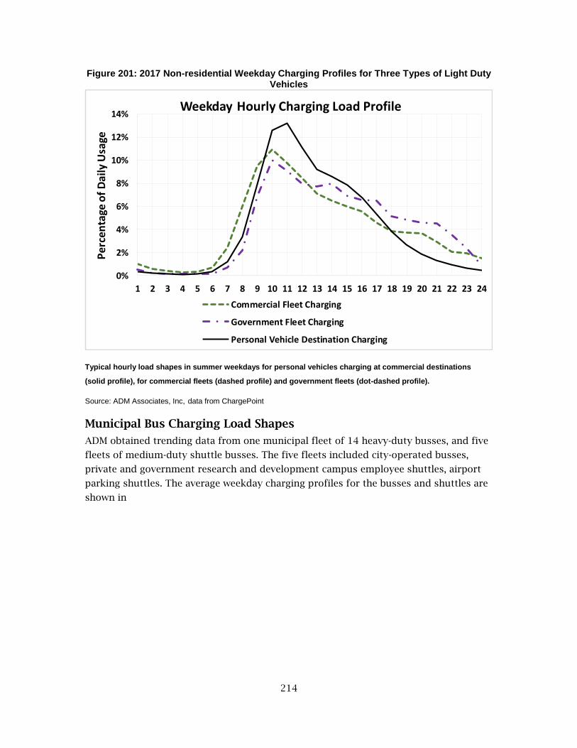
214
Figure 201: 2017 Non-residential Weekday Charging Profiles for Three Types of Light Duty Vehicles
Typical hourly load shapes in summer weekdays for personal vehicles charging at commercial destinations
(solid profile), for commercial fleets (dashed profile) and government fleets (dot-dashed profile).
Source: ADM Associates, Inc, data from ChargePoint
Municipal Bus Charging Load Shapes
ADM obtained trending data from one municipal fleet of 14 heavy-duty busses, and five
fleets of medium-duty shuttle busses. The five fleets included city-operated busses,
private and government research and development campus employee shuttles, airport
parking shuttles. The average weekday charging profiles for the busses and shuttles are
shown in
0%
2%
4%
6%
8%
10%
12%
14%
1 2 3 4 5 6 7 8 9 10 11 12 13 14 15 16 17 18 19 20 21 22 23 24
Per
cen
tage
of
Dai
ly U
sage
Weekday Hourly Charging Load Profile
Commercial Fleet Charging
Government Fleet Charging
Personal Vehicle Destination Charging

215
Figure 202.

216
Figure 202: 2018 Weekday Charging Profiles for Municipal Busses and Shuttle Fleets
Typical hourly load shapes in weekdays for heavy duty municipal busses (dark profile), and for shuttle fleets
(light profile).
Source: ADM Associates, Inc
Load Shape Specification and Creation
Light Duty Vehicles
Load shapes for light duty vehicles are developed from the ChargePoint data, as
discussed previously. The load shapes are developed by compiling average hourly
demand values for weekdays and weekend days for three types of locations: single
family residential, multifamily residential, and personal vehicle destination charging.
The hourly demand values are then normalized such that they sum to unity over all
hours of a typical (non-leap) year. The light duty vehicle load shapes are applied to the
portion of personal vehicle charging energy usage that occurs in the residential sector,
and to the entire energy use of neighborhood electric vehicles.
Medium/Heavy Duty Vehicles
Medium-duty and heavy-duty vehicles represent a small percentage of the overall
expected EV charging load. The group is heterogeneous in terms of operation and
charging demands and schedules, as can be inferred by inspection of Table 7. In this
table, the acronym GVWR denotes Gross Vehicle Weight Rating. Higher rating numbers
indicate heavier vehicles.
0%
1%
2%
3%
4%
5%
6%
7%
8%
1 2 3 4 5 6 7 8 9 10 11 12 13 14 15 16 17 18 19 20 21 22 23 24
Pere
nta
ge o
f Dai
ly E
ner
gy U
sage
Weekday Hourly Charging Load Profile
City_Bus Shuttle_Bus

217
Table 7: Listing of Medium and Heavy-Duty Vehicle Classes
Vehicle Type Typical Example Electric Variant Likely?
Distinct Charging Energy Forecast?
GVWR3
Possible Yes
GVWR4
Yes Combined with 5
GVWR5
Yes Combined with 4
GVWR-6
Possible Yes
GVWR7
Possible Yes
GVWR8 short-haul & Port
Yes Yes
GVWR8 garbage
Possible Yes
GVWR8 long-haul
Yes, Fixed Routes Only
No
Motorhomes (Class 3-7)
No No
City Bus (Class 7)
Yes Yes
School Bus (Class 6)
Yes Yes
Shuttle (Class 3)
Yes Yes
Description of medium and heavy-duty vehicles, whether an electric variant of the vehicle is likely, and whether a
separate value is currently being modeled for the vehicle-type.
Source: ADM Associates, Inc. https://afdc.energy.gov/data/10381

218
Although ADM was able to collect primary data for municipal busses and shuttles, data
for most of the categories above are not yet available. Even if distinct load shapes were
available, however, the multiplicity of distinct types would lead to data processing and
size issues. Given that medium and heavy-duty vehicles represent a small portion of the
2017 IEPR electric demand forecast for the transportation sector, the project team
sought to limit the number of load shapes assigned to this sector to three. This is
accomplished according to the grouping in Table 8.
Table 8: Grouping and Load Shape Construction for the Medium and Heavy-Duty Sector
Vehicle Type Typical Example Preliminary Load shape
GVWR3,4,5,6
50%/50% Blend of the Commercial Fleet LDV profile, and a flat profile.
GVWR7,8
40%/40%/20% blend of a flat profile, a simulated profile for refuse truck, and a simulated profile for a short haul semi-truck.
Bus
40%/40%/20% blend of a municipal bus profile, the shuttle fleet profile, and a simulated school bus profile.
Description of medium and heavy-duty vehicle grouping for the development of EV load shapes.
Source: ADM Associates, Inc.
The three load shapes used for this sector are described in the last column of Table 8.
The load shapes are blends of component profiles. Three of the component profiles—
refuse trucks, short haul semi-trucks, and school busses—are simulated according to

219
the assumption that charging occurs outside of the typical workday or school day. The
blended profiles for the three aggregated classes are shown in Figure 205.
Figure 203: 2018 Weekday Charging Profiles for Busses and Medium and Heavy-Duty Vehicles
Typical hourly load shapes in weekdays for medium duty trucks in GVWR ratings 3-6 (dot-dashed profile) for
heavy duty trucks (dashed profile), and for busses (solid profile).
Source: ADM Associates, Inc
Modeling Price Response Price response is modeled through application of elasticity factors. A load shape is
adjusted as follows:
𝐴ℎ = max (0,1 + 𝑇𝑂𝑈% × 𝑒 × (𝑃𝑅ℎ − 1))
Where:
𝐴ℎ is the adjustment factor for hour h
𝑇𝑂𝑈% is the percentage of customers that have a TOU rate
𝑃𝑅ℎ is the price ratio for hour h, defined as the price prevailing at hour h divided
by the lowest available price for the given day, at the same location
e is the Elasticity Factor
0%
1%
2%
3%
4%
5%
6%
7%
8%
9%
1 2 3 4 5 6 7 8 9 10 11 12 13 14 15 16 17 18 19 20 21 22 23 24
Per
cen
tage
of
Da
ily
Ener
gy U
sage
Weekday Hourly Charging Load Profile
GVWR3456 GVWR78 Bus

220
The max function sets a lower bound of zero for the adjustor14. The elasticity
normalization leads to reduced electric demand during high-price periods. To preserve
the overall forecast energy usage associated with charging, the load shapes are
renormalized to unity after the price elasticity adjustment. Note that the type of price
response modeled here is load shifting at the same location, rather than responding by
charging at an alternate location during the same or comparable time period. The latter
is addressed through adjustment of charging location shares for personal light duty
vehicles.
As an example, if 100% of the customers are on TOU rates, and the elasticity factor is -
0.7, and the price ratio is 2, then the adjustor is:
0.3 = (1 + 1 × −0.7 × (2 − 1))
This indicates that the demand is 30% of what it would have been in the absence of TOU
rates.
Elasticity factors are stored in a comma separated variable file, and take on separate
values by forecast zone, year, and customer sector. The factors may be adjusted by
Energy Commission staff. Default elasticity factors are -1.2 for the residential sector,
and -0.6 for the commercial sector.
Utility rate structures are also stored in a comma separated variable files and vary by
IOU and customer sector. The price response modeling occurs within the EV
Infrastructure Load Model, as described in the following section.
Determination of Default Price Elasticity Factors
ADM has placed default factors for elasticities: -1.2 for the residential sector and -0.6 for
the commercial sector. The factor for the residential sector was determined by
comparing charging session data as obtained from ChargePoint to data from the Joint
IOU report, as shown in Figure 204. The default elasticity factor for the commercial
sector is set to be half that of the residential sector. Both factors can be updated as
research results become available.
14 A dip below zero could be interpreted as customer’s willingness to act as a capacity source during a demand response event. Negative values are not considered in the model at his time.

221
Figure 204: Comparison of Summer Weekday Charging Profiles Developed from the Joint IOU Report and ChargePoint Data
Typical hourly load shapes in summer weekdays for single family homes as from the Joint IOU report (light solid
profile, averaged over all utilities) and ChargePoint (dark solid profile), and ChargePoint adjusted for price
elasticity (dashed profile).
Source: ADM Associates, Inc, data from PG&E, SCE, SDG&E, and ChargePoint
The ChargePoint data appear to show more on-peak usage than the profiles in the Joint
IOU Report, likely due to the fact that only a subset of ChargePoint customers are likely
to be on time of use rates. Rate information is not available in the ChargePoint data, but
the project team estimated that the fraction of ChargePoint customers on time of use
rates is 32% as follows.
ADM cross referenced the numbers of customers on EV TOU rates in the year 2017, as
reported in the Joint IOU Report (SDG&E, SCE & PG&E 2017), to the estimated number of
EV in IOU service territories for 2017, as reported in the Energy Commission’s Light
Duty Plug-In Energy and Emission Calculator. The Joint IOU Report tallies to
approximately 63,000 EV TOU accounts, compared to an estimated 266,000 EVs in
service by the end of 2017, as estimated by the Energy Commission calculator.15 Using
these values, ADM estimated roughly 23.7% of EV customers being on TOU rates.
Customers with EV specific TOU rates account for 1% of total residential accounts for
the IOUs. The Energy Commission estimates that about 9% of IOU customers were on
TOU rates in 2017. Assuming that about 1% of the 9% estimate is attributable to the EV
15 Sales in 2017 are estimated, actual Department of Motor Vehicles registration data from 2011-2016 are adjusted for attrition
0%
2%
4%
6%
8%
10%
12%
14%
16%
18%
1 2 3 4 5 6 7 8 9 10 11 12 13 14 15 16 17 18 19 20 21 22 23 24
Pe
rce
nt
of
Da
ily E
ne
rgy
USa
ge
Price Elasticity Calibration
IOUs (ChargePoint, 2017)IOUs (Joint IOU Report, 2017)CharePoint Data Adjusted for Elasticity
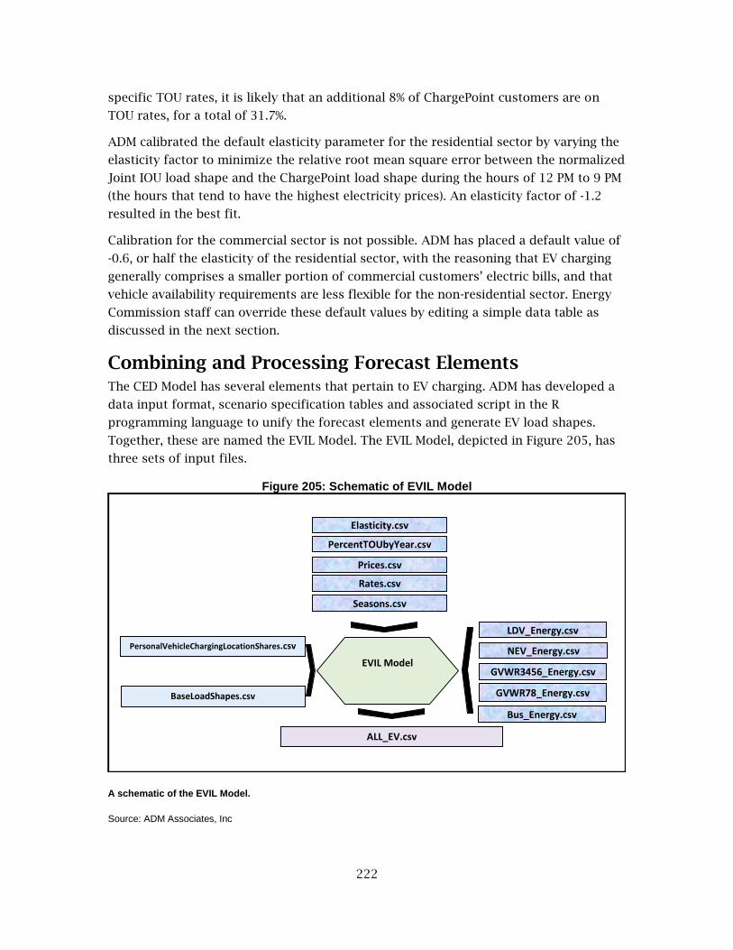
222
specific TOU rates, it is likely that an additional 8% of ChargePoint customers are on
TOU rates, for a total of 31.7%.
ADM calibrated the default elasticity parameter for the residential sector by varying the
elasticity factor to minimize the relative root mean square error between the normalized
Joint IOU load shape and the ChargePoint load shape during the hours of 12 PM to 9 PM
(the hours that tend to have the highest electricity prices). An elasticity factor of -1.2
resulted in the best fit.
Calibration for the commercial sector is not possible. ADM has placed a default value of
-0.6, or half the elasticity of the residential sector, with the reasoning that EV charging
generally comprises a smaller portion of commercial customers’ electric bills, and that
vehicle availability requirements are less flexible for the non-residential sector. Energy
Commission staff can override these default values by editing a simple data table as
discussed in the next section.
Combining and Processing Forecast Elements The CED Model has several elements that pertain to EV charging. ADM has developed a
data input format, scenario specification tables and associated script in the R
programming language to unify the forecast elements and generate EV load shapes.
Together, these are named the EVIL Model. The EVIL Model, depicted in Figure 205, has
three sets of input files.
Figure 205: Schematic of EVIL Model
A schematic of the EVIL Model.
Source: ADM Associates, Inc
LDV_Energy.csv
PersonalVehicleChargingLocationShares.csv
EVIL ModelNEV_Energy.csv
GVWR3456_Energy.csv
GVWR78_Energy.csv
Bus_Energy.csv
ALL_EV.csv
BaseLoadShapes.csv
Seasons.csv
Rates.csv
Prices.csv
PercentTOUbyYear.csv
Elasticity.csv

223
In the right of the diagram are a set of five input files that describe forecast energy
usages by vehicle classification, forecast zone, and year. The file LDV_Energy.csv,
corresponding to light duty vehicles, is the most detailed and accounts for the most
energy usage. The file includes one column to designate scenario, one column to
designate forecast zone, one column to designate the type of vehicle, and then a number
of columns that list forecast energy usages by year. Three types of vehicles are listed in
this file:
Personal vehicles—privately owned cars and light trucks
Commercial vehicles—cars and light trucks owned by businesses
Other vehicles—cars and light trucks owned by government entities, but also
include rental car fleets
In addition to the light duty plug-in electric vehicle forecast input file, there are four
files that describe forecast energy usages for neighborhood electric vehicles, trucks in
gross vehicle weight ratings three to six, trucks in gross vehicle weight ratings seven and
eight, and busses. It is assumed that these forecast elements are available by scenario
and year at the statewide level16.
At the top of Figure 205 figure are a set of five files that describe economic parameters
used in scenario analysis. The first file designates price elasticities for EV charging. The
elasticity factors are specified by year, forecast zone, and customer sector (commercial
and residential). The next four files concern forecast assumptions regarding time of use
rates. The file Seasons.csv defines seasons by month and utility company. The three
seasons are Summer, Winter, and “MarchApril”, which is necessitated by some SDG&E
rates that have special hour designations in March and April. The file Rates.csv assigns
the peak types for each rate, season, and day type (weekdays and weekends). The peak
types are standardized to the following:
Super off peak
Off peak
Mid peak
On peak
Critical peak
Each distinct rate assigns different hours to last four categories, although the hour
assignments are structurally similar with highest rates in summer afternoons and
lowest rates at nights. The critical peak designation is not currently in use but is
included in case critical peak pricing is to be modeled specifically for EV charging.
16 Conversations with Energy Commission staff indicate that a finer geographical resolution may be possible for certain forecast elements, although the most recent results are at the statewide level. The EVIL Model distributes impacts by zone in proportion to light duty vehicle energy usage.

224
Finally, the file Prices.csv assigns prices and price ratios to the peak types for each rate.
The price ratio is calculated as the ratio of the price in effect for a given hour, to the
lowest price available during the same day.
The remaining two input files are the load shapes, which are assumed to be static, but
can be updated as more data become available, and a file that distributes the total
charging energy requirement for personal light duty vehicles into the single family
residential, multifamily residential, and non-residential settings. The fractions can be
modified for each year. Current default values are 68.9% for the single-family residential
sector, 7.7% for the multifamily residential sector, and 23.4% for personal vehicle
destination charging in the commercial sector. These values were determined by
transcribing Figures 4.3 and 4.4 of the Energy Commission report California Plug-In
Electric Vehicle Infrastructure Projections: 2017-2025 CEC Staff Report and by assuming
that 90% of the charging in the residential sector occurs in single family homes (Bedir et
al. 2018).17
Output Format The EVIL model can output hourly loads associated with electric vehicle charging in
several formats. At the most detailed level, the model can produce hourly loads for the
entire forecast period. Although this is technically possible, the resulting data file can
approach 1 Gigabyte (GB) in size. The number of data element scale as the product of
each list element:
The number of years in the forecast (13 years if 2018-2030)
Three scenarios
8760 hours/year
12 forecast zones
Six distinct load shapes
A file that contains all of the above data would have 341,640 rows associated with the
scenarios and years, and 72 data columns with six load shapes per forecast zone.
It is important to recognize that the level of detail described is seldom necessary and by
default the EVIL model outputs data in a condensed format. ADM has identified several
ways to reduce file size while conveying the necessary information to Energy
Commission forecasters. The first step of data reduction is to sum over residential and
commercial sectors by zone. This reduces the six distinct load shapes to three, and
generates a three-fold data reduction. The second step is to recognize that the EV load
shapes for Monday to Friday are identical for any given month. Likewise, the profiles for
Saturdays and Sundays are identical. While this may not actually be true, it is a
necessary approximation. The rest of the forecast is largely weather dependent, while
17 Based on ADM’s understanding of the forecast process, the single family/multifamily distinction is relatively unimportant, as most forecast metrics are at the sector and zone level, or at higher levels.

225
EV charging is generally not weather dependent. The particular peak day for the forecast
is a function of the weather file, and not the day of the week (apart from the assumption
that the peak occurs on a non-holiday weekday). The best way to treat weather-
insensitive loads is in a probabilistic manner, which requires averaging over all
weekdays. This allows a 15-fold data compression, as one requires only two
representative days for each month.

226
CHAPTER 11: Energy Efficiency Load Impact Profiles
Application of Base Load Shapes and Energy Efficiency Load Impact Profiles to Scenario Analysis Base end-use load shapes, whole-building load shapes, and energy efficiency load impact
profiles will all be used to characterize hourly impacts from codes, standards, and
utility-sponsored energy efficiency programs. Much of the details surrounding the
assignment of load profiles to codes, standards, and efficiency forecast elements may be
automated with analysis scripts or spreadsheets. ADM has created a set of simple
scripts, precursors to the HELM 2.0, that couple specific impact forecasts to appropriate
load profiles. As one example, if a given AAEE forecast scenario expects 10 GWh of
savings for the commercial HVAC end-use in PG&E service territory, a set of scripts will
distribute the 10 GWh to all six forecast zones within PG&E service territory, and also to
each of the 12 commercial building types within each zone. Each building and zone
combination will be allotted a certain share of the overall 10 GWh in proportion to its
energy use within the overall commercial sector for PG&E. For each building type and
forecast zone, the total energy usage will also be divided into the major components
that are described by the ‘Commercial HVAC’ category in AAEE: Cooling, Heat Pumps,
Economizers, and Ventilation. The following sections motivate and describe this
process. The specific tables that map elements from AAEE and Committed Savings
forecast outputs to load shapes in HELM 2.0 are provided in Appendix B. Distribution of
statewide or planning area impacts to forecast zones and building types depend on the
base forecast output, year by year. The scripts that perform the disaggregation are
provided as an electronic attachment to this report.
Characterization of Energy Efficiency Load Impact Profiles Energy efficiency load impact profiles can be categorized as synchronous and
asynchronous to the load shape associated with the targeted end-use(s). The degree of
asynchronous behavior for a given energy efficiency measure will often determine the
appropriate source and construction process for the related load impact profile.
Synchronous Measures
As an example, an exterior lighting wattage reduction will have a load impact profile
that is synchronous with, and proportional to, the load shape for the targeted lights.
Synchronous measures (and their load impact profiles) are well-represented by the
associated end-use load shape. Some examples include:
Lighting wattage reductions in unconditioned space

227
HVAC system upgrades with systems that are more efficient, but not
qualitatively different than the baseline systems (e.g. heat pump vs. heat pump,
chiller vs. chiller)
Most residential and commercial refrigeration measures that increase
compressor efficiency or reduce thermal losses
Most appliances and electronics
Near Synchronous Measures
Some energy efficiency load impact profiles are nearly synchronous to the end-use load
shape. In many applications within the industry, the load shapes are taken as first order
approximations of these near-synchronous energy efficiency load impact profiles. Some
examples of near-synchronous measures are listed below:
Very high seasonal energy efficiency ratio (SEER) air conditioners or heat
pumps—typically variable speed or variable refrigerant flow systems—may have
very high coefficients of performance (COP), but only marginally higher energy
efficiency ratios (EER), which are more closely correlated with peak demand
savings.
Lighting wattage reductions in conditioned space are mildly asynchronous due to
HVAC interactive effects.
Heat pump water heaters will generally have higher relative energy savings
during summer than during winter, although most of the base energy usage
occurs during the cooler months.
In the residential sector, variable speed pool pumps tend to run longer hours,
but at lower speeds than single-speed pool pumps. A given pool pump upgrade
may have a load impact profile that differs from the load shape of either the
baseline or efficient pumps. A large collection of pool pump upgrades, however,
may be well-represented by the end-use load shape, as diversification tends to
distribute impacts across hours.
An example of a near synchronous energy efficiency load impact profile is provided in

228
Figure 206. Interior lighting wattage reductions in the commercial sector tend to have
similar shapes as the end-use load shape. However, reduced internal cooling loads due
to the lighting energy savings tend to decrease air conditioner run-times, resulting in
additional energy savings during the cooling season.

229
Figure 206: Comparison of Lighting Load Shape to Energy Efficiency Load Impact Profile
Typical hourly load shapes in July weekdays for interior lighting (solid profile) and interior lighting energy
efficiency (dashed profile) for offices in forecast zone 3. Cooling interactive effects tend to increase impacts –
particularly in afternoons.
Source: ADM Associates, Inc.
Asynchronous Measures
Other types of energy efficiency load impact profiles will typically have impacts that are
asynchronous to the load shapes of the targeted end-uses (Figure 209). Some examples
include:
Daylighting controls or lighting occupancy sensors
Envelope improvement measures such as efficient windows or added insulation.
Measures that involve fuel switching (for example air conditioner with a gas
furnace replaced with heat pump)
0
0.00002
0.00004
0.00006
0.00008
0.0001
0.00012
0.00014
0.00016
0.00018
0.0002
0 1 2 3 4 5 6 7 8 9 10 11 12 13 14 15 16 17 18 19 20 21 22 23
Perc
ent
of
An
nu
al E
ner
gy S
avin
gs
Hour Starting
Average Weekday Load Profile in July
Indoor.Lighting Indoor.Lighting.Eff

230
Figure 207: Comparison of Lighting Load Shape and Occupancy Sensor Load Impact Profile
Typical hourly load shape in May weekdays for interior lighting (solid profile) and energy efficiency load impact
profile for interior lighting occupancy sensor (dashed profile) for retail establishments in forecast zone 4. The
load impact profile is largely asynchronous with the underlying end-use load shape.
Source: ADM Associates, Inc.
Review of Potential and Goals Study, AAEE, and Committed Savings The CED Model includes 18 end-uses per zone for the residential sector and ten end-
uses per zone for each of 12 building types in the commercial sector. Other sectors are
considered at the whole building level. Potential energy efficiency measures, however,
number in the hundreds for a given zone and building type combination. CED Model
components for AAEE and committed savings, on the other hand, are at the sector and
end-use level—a lower level of resolution than the demand forecast which is justified by
the relatively small impact of energy efficiency compared to overall demand. ADM
strove to balance the staggering multiplicity of individual energy efficiency measures
described in the Potential and Goals Study18, with the relatively low resolution of AAEE
and committed savings forecast elements.
18 Wikler et al. 2017. Energy Efficiency Potential and Goals Study for 2018 and Beyond. California Public Utilities Commission. Reference Number: 174655
0
0.00005
0.0001
0.00015
0.0002
0.00025
0 1 2 3 4 5 6 7 8 9 10 11 12 13 14 15 16 17 18 19 20 21 22 23
Perc
ent
of A
nn
ual
En
ergy
Sav
ings
Hour Starting
Average WeekdayLoad Profile in May
Indoor.Lighting Occupancy Sensors

231
To identify the key sectors, end-uses, and measures to represent AAEE and committed
savings, ADM reviewed the recent AAEE forecast elements from the 2017 Integrated
Energy Policy Report (Bahreinian et al. 2018). The 2017 forecast included six AAEE
scenarios. As a first step, ADM investigated the various agents of expected energy
efficiency. As shown in Figure 208, in each of six forecast scenarios, utility-sponsored
energy efficiency programs are expected to account for the most energy savings. Federal
appliance standards are the next most significant component, followed by building
standards.
Figure 208: Total AAEE Energy Savings by Category and Scenario
AAEE energy savings by savings category and scenario, taken from the 2017 Integrated Energy Policy Report
(Bahreinian et al., 2018). Most impacts are concentrated in utility-sponsored programs and federal appliance
standards.
Source: ADM Associates, Inc.
Utility-sponsored programs, federal appliance standards and existing building standards
are described with relatively high resolution. Smaller components, such as future
building standards or yet-undetermined legislatively-induced energy savings, are not
specified in a manner to allow assignment of closely matched load shapes.
As a next step, ADM inspected the relative weight of overall energy savings by customer
sector for each forecast scenario. In all scenarios, most energy savings accrue to the
commercial sector, followed by the residential sector. All other sectors combined
account for less than 15% of savings, in each scenario.
0%
10%
20%
30%
40%
50%
60%
70%
Low (Scenario 1)
Low (Scenario 2)
Mid (Scenario 3)
High (Scenario 4)
High (Scenario 5)
High Plus(Scenario 6)
Perc
enta
ge o
f Res
iden
tial
En
ergy
Sav
ings
AAEE Total Energy Savings by Category and Scenario
Utility Programs Appliance Standards Building Standards
SB 350 - Bldg Stnds SB 350 - Appl Stnds SB 350 - Other

232
Figure 209: Total AAEE Energy Savings by Sector and Scenario, from the 2017 Integrated Energy Policy Report
AAEE energy savings by customer sector and scenario, taken from the 2017 Integrated Energy Policy Report
(Bahreinian et al. 2018). Most impacts are concentrated in the commercial and residential sectors.
Source: ADM Associates, Inc.
Given the importance of commercial and residential sectors, ADM looked more closely
at the forecast AAEE savings for these two sectors.
Commercial Sector
In the commercial sector, much of the energy savings are attributable to lighting, HVAC,
and refrigeration, as shown in
0%
10%
20%
30%
40%
50%
60%
70%
80%
Low (Scenario 1)
Low (Scenario 2)
Mid (Scenario 3)
High (Scenario 4)
High (Scenario 5)
High Plus(Scenario 6)Pe
rcen
tage
of O
vera
ll En
ergy
Sav
ings
AAEE Energy Savings by Sector and Scenario
com res ag ind stl

233
Figure 210. However, as the AAEE scenarios become more aggressive, energy efficiency
that target the whole building, rather than any particular end-use, become more
significant. Most of the energy savings in the whole building category are attributable to
building standards and utility sponsored behavioral programs.

234
Figure 210: AAEE Commercial Energy Savings by End-Use and Scenario
Commercial AAEE energy savings by end-use and scenario, taken from the 2017 Integrated Energy Policy Report
(Bahreinian et al. 2018). Most impacts are concentrated in the lighting, HVAC, refrigeration, and whole building
savings.
Source: ADM Associates, Inc.
Additional detail at the measure level is available in the appendices of the Potential and
Goals Study (Wilker et al., 2017)19. ADM reviewed savings contributions of specific
measures for the three most significant end-uses in the commercial sector. The results
for utility-sponsored programs are shown in
Figure 211. Codes and standards based energy savings have similar patterns. It is
interesting to note that most of the energy savings are attributable to efficiency
improvements, such as lighting wattage reductions or more efficient compressors,
rather than controls-based measures such as variable frequency drives or occupancy
sensors. This is consistent with the project team’s experience from evaluating
commercial and industrial energy efficiency programs across the country.
19 ADM found the following excel summary to be particularly helpful: ftp://ftp.cpuc.ca.gov/gopher-data/energy_division/EnergyEfficiency/DAWG/2018_PG%20Study%20Measure%20Level%20Results%20Final_092517.xlsx
0%
10%
20%
30%
40%
50%
60%
Low (Scenario 1)
Low (Scenario 2)
Mid (Scenario 3)
High (Scenario 4)
High (Scenario 5)
High Plus(Scenario 6)Pe
rcen
tage
of C
om
mer
cial
En
ergy
Sa
vin
gsAAEE Commercial Energy Savings by End Use and Scenario
Lighting HVAC Refrigeration Whole Building Plug Loads Other

235
Figure 211: Utility Program Savings by Specific Measure for Major End-Uses in the Commercial Sector
Utility-sponsored commercial sector energy savings for the lighting, HVAC, and refrigeration end-uses, lighting,
HVAC, and refrigeration end-uses, broken down into specific measures by inspecting the Potential and Goals
Study measure level results viewer for the ‘mTRC (GHG adder 1)’ scenario.
Source: ADM Associates, Inc.
Based on the previous findings summarized, ADM identified much of the energy savings
associated with outdoor lighting, HVAC, and refrigeration area characterized as
synchronous, and can be represented with corresponding end-use load shapes. A special
load impact profile is warranted for indoor lighting, as it is the most significant energy
savings component, and the impacts are near-synchronous, but not synchronous with
the end-use load shape. ADM also developed separate energy efficiency load impact
profiles for daylighting and occupancy sensors, as these are asynchronous measures
which are not well-represented by the end-use load shape. For HVAC energy efficiency
measures, ADM developed economizer and heat pump energy efficiency load impact
profiles. A heat pump energy efficiency load impact profile is necessary primarily
because the heating and cooling end-use load shapes are treated as separate end-uses,
while a heat pump will save on both end-uses, with the fraction of heating and cooling
savings varying by building type and geographical location. ADM also developed whole
building energy efficiency load impact profiles, which can be used to represent
behavioral programs and expected but unspecified building standards. Finally, a “flat”
energy efficiency load impact profile was provided to represent savings for various
energy efficiency measures that are essentially constant in impacts, such as parking
garage lighting upgrades, efficient data centers, and (as a good approximation) process-
93%6%
1%
0%
UTILITY PROGRAM COMMERCIAL LIGHTING SAVINGS
Indoor Lighting Outdoor Lighting
Controls Other
75%
10%
13%
2%
UTILITY PROGRAM COMMERCIAL HVAC SAVINGS
Chiller/AC Economizer Heat Pump Other
44%
41%7%
8%
UTILITY PROGRAM COMMERCIAL REFRIGERATION SAVINGS
Efficient Cases/Compressors
Fans / Lights
Floating Head Pressure
Other

236
related air compressors. Table 9 lists base and efficiency load shapes for the commercial
sector.
Table 9: List of Load Shapes Used to Model Commercial Sector AAEE Savings
Base End-use Load Shapes
Energy Efficiency Load Impact Profiles
Daylighting
Occupancy Sensor
Heating Refrigeration Lighting Efficiency
Cooling Indoor Lighting Heat Pump
Ventilation Miscellaneous Economizer
Water Heating Office Equipment Whole Building
Cooking Outdoor Lighting Flat
A list of base and efficiency load shapes for the commercial sector.
Source: ADM Associates, Inc.
Residential Sector
In the residential sector, much of the energy savings are also attributable to lighting,
whole building, and plug loads, as shown in Figure 212. However, as the AAEE scenarios
become more aggressive, lighting comprises a smaller portion of the savings while other
measures become more significant. Most of the energy savings in the “other” category is
attributable to building standards and utility sponsored behavioral programs.
Figure 212: AAEE Residential Energy Savings by End-Use and Scenario
Residential AAEE energy savings by end-use and scenario, taken from the 2017 Integrated Energy Policy Report
(Bahreinian et al., 2018). Most impacts are concentrated in the lighting, plug loads, and whole-building.
0%
5%
10%
15%
20%
25%
30%
35%
40%
45%
50%
Low (Scenario 1)
Low (Scenario 2)
Mid (Scenario 3)
High (Scenario 4)
High (Scenario 5)
High Plus(Scenario 6)
Perc
enta
ge o
f Res
iden
tial
En
ergy
Sa
vin
gs
AAEE Residential Energy Savings by End Use and Scenario
Lighting Whole Building Plug Loads HVAC Other
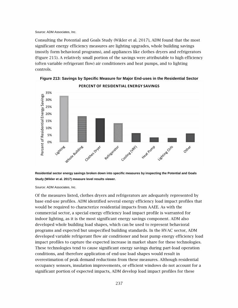
237
Source: ADM Associates, Inc.
Consulting the Potential and Goals Study (Wikler et al. 2017), ADM found that the most
significant energy efficiency measures are lighting upgrades, whole building savings
(mostly form behavioral programs), and appliances like clothes dryers and refrigerators
(Figure 215). A relatively small portion of the savings were attributable to high efficiency
(often variable refrigerant flow) air conditioners and heat pumps, and to lighting
controls.
Figure 213: Savings by Specific Measure for Major End-uses in the Residential Sector
Residential sector energy savings broken down into specific measures by inspecting the Potential and Goals
Study (Wikler et al. 2017) measure level results viewer.
Source: ADM Associates, Inc.
Of the measures listed, clothes dryers and refrigerators are adequately represented by
base end-use profiles. ADM identified several energy efficiency load impact profiles that
would be required to characterize residential impacts from AAEE. As with the
commercial sector, a special energy efficiency load impact profile is warranted for
indoor lighting, as it is the most significant energy savings component. ADM also
developed whole building load shapes, which can be used to represent behavioral
programs and expected but unspecified building standards. In the HVAC sector, ADM
developed variable refrigerant flow air conditioner and heat pump energy efficiency load
impact profiles to capture the expected increase in market share for these technologies.
These technologies tend to cause significant energy savings during part-load operation
conditions, and therefore application of end-use load shapes would result in
overestimation of peak demand reductions from these measures. Although residential
occupancy sensors, insulation improvements, or efficient windows do not account for a
significant portion of expected impacts, ADM develop load impact profiles for these
0%
5%
10%
15%
20%
25%
30%
35%
Perc
ent
of R
esid
enti
al E
ner
gy S
avin
gs
PERCENT OF RESIDENTIAL ENERGY SAVINGS

238
measures for completeness, as these measures are asynchronous with the end-use load
shape and are not well represented.

239
Table 10 lists end-use load shapes and energy efficiency load impact profiles for the
residential sector.

240
Table 10: List of Load Shapes Used to Model Residential Sector AAEE Savings
Base End-use Load Shapes Energy Efficiency Load
Impact Profiles Cooking Pool Heater
Cooling Pool Pump
Dishwasher Refrigerator Whole Building
Dryer Solar Pool Pump Insulation
Freezer Spa Heater Lighting Efficiency
Furnace Fan Spa Pump Efficient Windows
Heating Television Heat Pump (high SEER/VRF)
Lighting Washer Cooling (high SEER/VRF)
Miscellaneous Water Heater Occupancy Sensor
A list of base and efficiency load shapes for the residential sector.
Source: ADM Associates, Inc.
Other Sectors
The TCU, mining and extraction, and industrial sectors are described only with whole
building end-use load shapes. Accordingly, whole building load shapes are also used to
characterize AAEE and committed savings for these sectors. The streetlighting sector is
described with one load impact profile, which serves as the end-use profile and the
energy efficiency load impact profile.
Additional Considerations in Load Impact Profile Selection
The energy efficiency load impact profiles in the last columns of Table 9 and

241
Table 10 are winnowed from a broader list of candidate load impact profiles. ADM
made the following considerations to retain or discard candidate profiles:
1. Does the candidate load impact profile correspond well to measures that
describe a significant portion of energy savings described in the Potential and
Goals Study (Wikler et al., 2017)?
2. Does the candidate load impact profile represent a significant improvement over
the best matching end-use load shape? For example, is it asynchronous with the
targeted end-use?
3. Are there sufficient data or simulation tools to construct the candidate profile?
4. Are there any other candidate load impact profiles that can serve the same
purpose?
The above considerations are demonstrated in an example below. The example involves
utility company sponsored energy savings for the HVAC end-use in the commercial
sector. Table 11 lists the energy efficiency measures that account for the top 95% of
energy savings through the year 2030 associated with utility-sponsored programs. The
last column shows candidate load shape assignment. In the project naming convention,
load impact profiles that have been developed specifically for use as energy efficiency
load impact profiles have the “.Eff” suffix.
Table 11: Measures in the Potential and Goals Study that Account for the Top 95% of Commercial HVAC Energy Savings
Utility Sponsored Program Measure Percent of Total Energy Savings
Candidate Load Impact Profile
Com | Split System AC (SEER 22) 26% Cooling
Com | Efficient Chiller 16% Cooling
Com | Split System AC (SEER 18) 15% Cooling
Com | Split System AC (SEER 16) 14% Cooling
Com | Economizer 10% Economizer.Eff
Com | HVAC Quality Maintenance (Elec SH) 9% Heat.Pump.Eff
Com | Split System AC (SEER 14) 2% Cooling
Com | Packaged RTU AC (IEER 14.0) 1% Cooling
Com | Ductless Mini Split Heat Pump (SEER 18) 1% Heat.Pump.Eff
Com | HVAC Motor - ECM 1% Ventilation
List of measures in the Potential and Goals Study that account for the top 95% of the commercial HVAC energy
savings projected through 2030 and their respective candidate load impact profiles.
Source: ADM Associates, Inc.
After assigning candidate load shapes to each listed measure (including a number of
measures not listed above, that account for the last 5% of energy savings), the candidate
load impact profiles are assessed by reviewing the total energy savings represented by
load shape, as shown in Table 12.
Table 12: Percent of Overall Commercial HVAC Energy Savings by Candidate Load Shape

242
Candidate Load Shape Percent of Savings
Cooling 75.01%
Heat.Pump.Eff 12.60%
Economizer.Eff 9.91%
Thermostat.Eff 1.64%
Ventilation 0.81%
Ground.Source.Heat.Pump.Eff 0.01%
List of contribution to commercial HVAC savings by candidate load shape.
Source: ADM Associates, Inc.
Referring to Table 12, a quick observation is that the Ground.Source.Heat.Pump.Eff
candidate load impact profile, which represents ground source heat pumps, is distinct
from the overall Heat.Pump.Eff profile which represents efficient air source heat pumps.
Ground source heat pumps have different part-load curves than air-source heat pumps.
Notably, they have distinct advantages during extreme temperatures. The expected
energy savings from ground source heat pumps amounts to 0.01% of the total for the
HVAC end-uses, however. Applying the four considerations above, it can be concluded
that:
1. The ground source heat pump candidate load shape does not represent a
significant portion of the expected energy savings.
2. The ground source heat pump candidate load shape offers an advantage over the
existing end-use profile. In fact, there is no heat-pump end-use profile, only
heating, cooling, and ventilation.
3. The ground source heat pump energy efficiency measure can be simulated
within the EnergyPlus framework.
4. The Heat.Pump.Eff candidate profile would be quite similar to a ground source
heat pump profile, and solves the problem identified in item #2 above.
After the four considerations above, ADM decided to discard the ground source heat
pump candidate load impact profile and to re-assign its weight to air source heat
pumps.
The same considerations are applied to the thermostat and ventilation candidate load
impact profiles. ADM found that smart thermostats cannot reliably be simulated by
EnergyPlus, and also that they represent a small portion of the overall savings. ADM
selected the ventilation end-use load shape as a reasonable proxy. The economizer and
heat pump candidate energy efficiency profiles were generated in the EnergyPlus/R
framework as described in the next section.
Development of Energy Efficiency Load Impacts ADM utilized the same EnergyPlus/R framework that was used to develop load shapes
to develop most of the energy efficiency load impact profiles. The basic process is
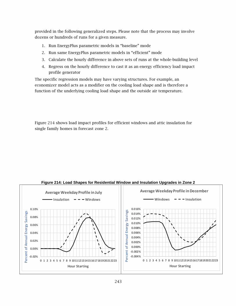
243
provided in the following generalized steps. Please note that the process may involve
dozens or hundreds of runs for a given measure.
1. Run EnergyPlus parametric models in “baseline” mode
2. Run same EnergyPlus parametric models in “efficient” mode
3. Calculate the hourly difference in above sets of runs at the whole-building level
4. Regress on the hourly difference to cast it as an energy efficiency load impact
profile generator
The specific regression models may have varying structures. For example, an
economizer model acts as a modifier on the cooling load shape and is therefore a
function of the underlying cooling load shape and the outside air temperature.
Figure 214 shows load impact profiles for efficient windows and attic insulation for
single family homes in forecast zone 2.
Figure 214: Load Shapes for Residential Window and Insulation Upgrades in Zone 2
-0.02%
0.00%
0.02%
0.04%
0.06%
0.08%
0.10%
0 1 2 3 4 5 6 7 8 9 1011121314151617181920212223Per
cen
t o
f A
nn
ua
l En
ergy
Sa
vin
gs
Hour Starting
Average Weekday Profile in July
Insulation Windows
-0.004%
-0.002%
0.000%
0.002%
0.004%
0.006%
0.008%
0.010%
0.012%
0.014%
0.016%
0 1 2 3 4 5 6 7 8 9 1011121314151617181920212223Per
cen
t o
f A
nn
ua
l En
ergy
Sa
vin
gs
Hour Starting
Average Weekday Profile in December
Windows Insulation

244
Energy efficiency load impact profiles for single family residences in forecast zone 2 for attic insulation (solid
profile) and efficient windows (dashed profile) in July (left plot) and December (right plot).
Source: ADM Associates, Inc.
Lighting Occupancy Sensor Load shapes
The process above describes the development effort for most energy efficiency load
shapes. The lighting occupancy sensor load shapes, however, required significant data
collection and processing in advance of running the EnergyPlus models. To estimate
energy efficiency load impact profiles for occupancy sensors, ADM reviewed lighting
logger data from hundreds of lighting loggers installed for measurement and
verification of energy efficiency programs across the country. Each of the data loggers
was installed on a fixture that was controlled by an occupancy sensor. ADM imputed the
baseline schedule, following a process that ADM has devised for measurement and
verification of commercial lighting projects, and then determined hourly multipliers for
weekdays and weekends. For example, a multiplier of 0.7 indicates that occupancy
sensors achieve a 30% on-time reduction for a given hour. The multipliers were then
applied to base load shapes by matching annual hours’ baseline hours of use to building
types based on typical operation profiles. In this step, logger data were categorized into
short, medium, or long hours of use, and schools and offices were assigned the savings
factors from loggers with shorter hours of use, college and retail were assigned medium
hours of use, and all other building types were assigned the savings factors derived
from loggers that had longer hours of use. The modified base load shapes were then fed
into EnergyPlus simulations described previously.
Lighting occupancy sensors represent a much smaller portion of residential sector
energy savings. Despite having conducted lighting metering studies, ADM did not have
primary data available to characterize the impacts of occupancy sensors. ADM
developed a residential lighting occupancy sensor profile by assuming that a
disproportionate amount of the energy savings occurs during times that are associated
with declines in lighting use (8 PM to 3 AM). The savings profile was then put through
the four-step process listed above to add interactive effects (Figure 217).
Figure 215: Residential Lighting Load Shape, Lighting Efficiency Impact Profile, and Occupancy Sensor Impact Profile
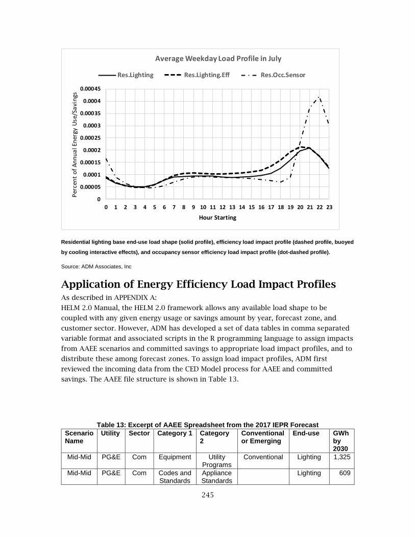
245
Residential lighting base end-use load shape (solid profile), efficiency load impact profile (dashed profile, buoyed
by cooling interactive effects), and occupancy sensor efficiency load impact profile (dot-dashed profile).
Source: ADM Associates, Inc
Application of Energy Efficiency Load Impact Profiles As described in APPENDIX A:
HELM 2.0 Manual, the HELM 2.0 framework allows any available load shape to be
coupled with any given energy usage or savings amount by year, forecast zone, and
customer sector. However, ADM has developed a set of data tables in comma separated
variable format and associated scripts in the R programming language to assign impacts
from AAEE scenarios and committed savings to appropriate load impact profiles, and to
distribute these among forecast zones. To assign load impact profiles, ADM first
reviewed the incoming data from the CED Model process for AAEE and committed
savings. The AAEE file structure is shown in Table 13.
Table 13: Excerpt of AAEE Spreadsheet from the 2017 IEPR Forecast
Scenario Name
Utility Sector Category 1 Category 2
Conventional or Emerging
End-use GWh by 2030
Mid-Mid PG&E Com Equipment Utility Programs
Conventional Lighting 1,325
Mid-Mid PG&E Com Codes and Standards
Appliance Standards
Lighting 609
0
0.00005
0.0001
0.00015
0.0002
0.00025
0.0003
0.00035
0.0004
0.00045
0 1 2 3 4 5 6 7 8 9 10 11 12 13 14 15 16 17 18 19 20 21 22 23
Per
cen
t o
f A
nn
ua
l En
ergy
Use
/Sa
vin
gs
Hour Starting
Average Weekday Load Profile in July
Res.Lighting Res.Lighting.Eff Res.Occ.Sensor

246
Mid-Mid PG&E Com SB 350 - Prop 39
Prop 39 Lighting 46
Mid-Mid PG&E Com Equipment Utility Programs
Emerging Lighting 8
An excerpt of the AAEE spreadsheet from the 2017 IEPR Forecast which illustrates the GWh savings projected
for commercial lighting.
Source: ADM Associates, Inc.
The energy savings are characterized by end-use and also by two categories. Recall that
utility programs account for most of the expected energy savings and that the
remaining categories are largely due to codes and standards, notably federal appliance
standards and California building standards. ADM combined the three data fields
Category 1, Category 2, and Conventional or Emerging as follows: Any line item that is
described as a utility program under Category 2 is designated as “Utility” and all other
line items are categorizes as “Other”, with the understanding that the “Other” category
is dominated by codes and standards. ADM then consulted the Measure Level Results
Appendix of the Potential and Goals Study (Wikler et al. 2017), and reviewed the utility
sponsored measures and the codes and standards measures for each end-use and
sector. Note that the Potential and Goals Study also includes behavioral programs, but
the impacts from behavioral programs are modeled with whole building load impact
profiles rather than end-use specific profiles. Table 14 demonstrates how load impact
profiles are assigned to the two middle rows of Table 13. ADM used six distinct load
impact profiles that may characterize energy savings for commercial lighting. ADM
assigned weights to load impact profiles for each code-based energy efficiency measure.
The weights in each row sum to 100%. For example, 100% of the sky-lighting measure is
described with the Daylighting.Eff load impact profile, while the non-residential
alterations are distributed to indoor and outdoor lighting, occupancy sensors, and
daylighting.

247
Table 14: Load Shape Assignment for Commercial Lighting Codes and Standards
Codes and Standards Measure for Commercial Lighting
Indo
or.
Lig
hting
.Eff
Outd
oor.
Lig
hting
Daylig
hting.E
ff
Occsensor.
Eff
Fla
t
2013 T-24: NRA-Lighting-Alterations-New Measures 80% 10% 1% 9% 0%
2013 T-24: NRA-Lighting-Alterations-Existing Measures 80% 10% 1% 9% 0%
2013 T-24: NRA-Lighting-Egress Lighting Control 5% 5% 0% 90% 0%
Future T-20: Small Diameter Directional Lamps (Tier 1) 100% 0% 0% 0% 0%
2016 T-24 -NRA-Lighting-Alterations 80% 10% 1% 9% 0%
2013 T-24: NRNC-Lighting-Controllable Lighting 0% 0% 10% 90% 0%
2013 T-24: NRNC-Lighting-Egress Lighting Control 5% 5% 0% 90% 0%
2013 T-24: NRA-Lighting-Warehouses and Libraries 80% 10% 1% 9% 0%
Fed Appliance: General Service Fluorescent Lamps #2 95% 5% 0% 0% 0%
2008 T-24: Tailored Indoor lighting 100% 0% 0% 0% 0%
2013 T-24: NRNC-Lighting-Warehouses and Libraries 80% 3% 2% 15% 0%
2008 T-24: Skylighting 0% 0% 100% 0% 0%
Fed Appliance: General Service Fluorescent Lamps #1 95% 5% 0% 0% 0%
2013 T-24: NRNC-Lighting-Office Plug Load Control 0% 0% 0% 100% 0%
Fed Appliance: Fluorescent Ballasts 95% 5% 0% 0% 0%
2013 T-24: NRNC-Lighting-Parking Garage 0% 0% 0% 0% 100%
2008 T-24: Sidelighting 10% 0% 90% 0% 0%
2016 T-20: Dimming Ballasts 25% 25% 25% 25% 0%
2013 T-24: NRNC-Lighting-MF Building Corridors 0% 0% 0% 0% 100%
2013 T-24: NRNC-Lighting-Outdoor Lighting & Controls 0% 100% 0% 0% 0%
2013 T-24: NRA-Lighting-MF Building Corridors 0% 0% 0% 0% 100%
2008 T-24: Outdoor Lighting 0% 100% 0% 0% 0%
Fed Appliance: Metal Halide Lamp Fixtures 50% 50% 0% 0% 0%
2016 T-24 -NRA-Lighting-ASHARE Measure-Elevator Lighting & Ventilation
0% 0% 0% 0% 100%
2016 T-24 -NRA-Lighting-Outdoor Lighting Controls 0% 100% 0% 0% 0%
2013 T-24: NRA-Lighting-Hotel Corridors 0% 0% 0% 0% 100%
2005 T-24: Lighting controls under skylights 0% 0% 100% 0% 0%
A list of commercial lighting codes and standards reported in the Potential and Goals Study and their relative
assignment to ADM’s lighting-related energy efficiency load impact profiles.
Source: ADM Associates, Inc.
The weights in the above table were developed based on expert judgment of ADM staff
with extensive experience in commercial lighting projects, particularly in new
construction applications. It is important to note, however, that the weights shown
herein are fed into simple load-shape assignment tables and can be readily updated by
Commission Staff if needed. The tables for AAEE and committed savings are provided in
Appendix B.
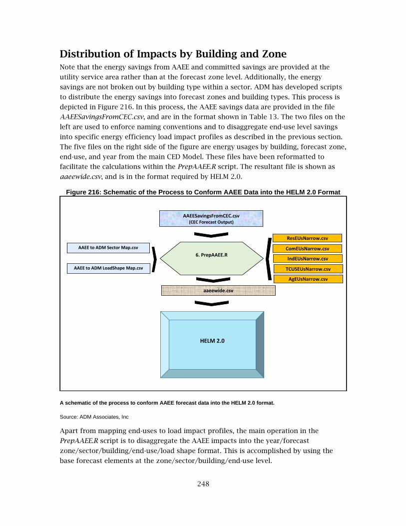
248
Distribution of Impacts by Building and Zone Note that the energy savings from AAEE and committed savings are provided at the
utility service area rather than at the forecast zone level. Additionally, the energy
savings are not broken out by building type within a sector. ADM has developed scripts
to distribute the energy savings into forecast zones and building types. This process is
depicted in Figure 216. In this process, the AAEE savings data are provided in the file
AAEESavingsFromCEC.csv, and are in the format shown in Table 13. The two files on the
left are used to enforce naming conventions and to disaggregate end-use level savings
into specific energy efficiency load impact profiles as described in the previous section.
The five files on the right side of the figure are energy usages by building, forecast zone,
end-use, and year from the main CED Model. These files have been reformatted to
facilitate the calculations within the PrepAAEE.R script. The resultant file is shown as
aaeewide.csv, and is in the format required by HELM 2.0.
Figure 216: Schematic of the Process to Conform AAEE Data into the HELM 2.0 Format
A schematic of the process to conform AAEE forecast data into the HELM 2.0 format.
Source: ADM Associates, Inc
Apart from mapping end-uses to load impact profiles, the main operation in the
PrepAAEE.R script is to disaggregate the AAEE impacts into the year/forecast
zone/sector/building/end-use/load shape format. This is accomplished by using the
base forecast elements at the zone/sector/building/end-use level.
ResEUsNarrow.csv
6. PrepAAEE.RComEUsNarrow.csv
IndEUsNarrow.csv
TCUSEUsNarrow.csv
AgEUsNarrow.csv
HELM 2.0
aaeewide.csv
AAEE to ADM Sector Map.csv
AAEE to ADM LoadShape Map.csv
AAEESavingsFromCEC.csv(CEC Forecast Output)

249
For a given sector and end-use, the weights at the building and forecast zone level are
calculated as follows:
𝑊𝑒𝑖𝑔ℎ𝑡𝐵𝑍 = ∑ 𝐺𝑊ℎ𝑈,𝑆,𝑌,𝐵,𝑍
∑ 𝐺𝑊ℎ𝑈,𝑆,𝑌
Where:
U denotes utility service territory
S denotes sector
Y denotes year
B denotes building type
Z denotes forecast zone.
For example, if large offices in forecast zone 1 are expected to account for 3% of the
energy use for the PG&E service territory in 2020, the team expects 3% of the energy
savings to also accrue to large offices.
ADM has developed a similar process for committed energy savings. As of this writing,
the Energy Commission is updating the CED Model, and it is possible that the updated
model may provide AAEE and committed savings data at the same resolution as the load
forecast. The scripts and map files are provided to Energy Commission staff in case the
AAEE and committed savings will continue to be developed as they have been for the
2017 forecast.

250
REFERENCES Abrishami, Mohsen, Sylvia Bender, Kae C. Lewis, Nahid Movassagh, Peter Puglia, Glen
Sharp, Kate Sullivan, Mitch Tian, Belen Valencia, and David Videvar (California
Energy Commission), 2005. Energy Demand Forecast Methods Report:
Companion Report to the California Energy Demand 2006-2016 Staff Energy
Demand Forecast Report. California Energy Commission. Publication Number:
CEC-400-2005-036.
Bahreinian, Aniss, Stephanie Bailey, Jim Bartridge, Leon Brathwaite, Jennifer Campagna,
Noel Crisostomo, Pamela Doughman, Tom Flynn, Guido Franco, Judy Grau, Mike
Gravely, Eli Harland, Elizabeth John, Melissa Jones, Chris Kavalec, Matthew Ong,
Charles Smith, Michael Sokol, and Lana Wong (California Energy Commission),
2018. 2017 Integrated Energy Policy Report. California Energy Commission.
Publication Number: CEC-100-2017-001-CMF.
Bedir, Abdulkadir, Noel Crisostomo, Jennifer Allen, Eric Wood, and Clément Rames.
2018. California Plug-In Electric Vehicle Infrastructure Projections: 2017-2025.
California Energy Commission. Publication Number: CEC-600-2018-001.
California Energy Commission, 2016. California Investor-Owned Utility Electricity Load
Shapes. California Energy Commission. Publication Number: RFP-15-322.
De León, S., S. Leno, A. Williams, S. Allen, S. Hancock, A. McCarty, and S. Monning, 2015.
SB-350 Clean Energy and Pollution Reduction Act of 2015. State of California
Legislative Counsel Bureau.
Electric Power Research Institute (EPRI), 2016. Load Shape Library 4.0.
http://loadshape.epri.com/
Energy and Environmental Economics, Inc. (E3), 2005. Energy Efficiency Calculator.
https://www.ethree.com/public_proceedings/energy-efficiency-calculator/
Energy Solutions, 2016. California Distributed Generation Statistics. California Public
Utilities Commission. https://www.californiadgstats.ca.gov/
GDS Associates, Inc., Nexant, Research Into Action, and Apex Analytics (Statewide
Evaluation Team), 2014. Pennsylvania Statewide Act 129: 2014 Commercial &
Residential Light Metering Study. Pennsylvania Public Utilities Commission.
Grist, Charlie (Northwest Power & Conservation Council), 2016. End Use Load Research
in the Pacific Northwest: Why Now?
https://conduitnw.org/_layouts/Conduit/FileHandler.ashx?rid=3280
Her Majesty’s Nautical Almanac Office, 2012. The Astronomical Data Portal @ UK
Hydrographic Office. UK Hydrographic Office. http://astro.ukho.gov.uk/
Itron, Inc., 2006. California Commercial End-Use Survey. California Energy
Commission. Publication Number: CEC-400-2006-005.

251
Itron, Inc., 2011. DEER Database: 2011 Update Documentation. California Public
Utilities Commission.
League of Oregon Cities, 2010. Street and Traffic Lighting: Survey of Oregon Cities
Fall 2010. League of Oregon Cities.
Pacific Northwest National Laboratory (PNNL), 2018. Commercial Prototype Building
Models. The U.S. Department of Energy.
https://www.energycodes.gov/development/commercial/prototype_models
Palmgren, Claire, Noel Stevens, Miriam Goldberg, Ph.D., Rich Barnes, and Karen Rothkin,
Ph.D (KEMA, Inc.), 2010. 2009 California Residential Appliance Saturation Study.
California Energy Commission. Publication Number: CEC-200-2010-004.
San Diego Gas & Electric Company, Southern California Edison Company, and Pacific Gas
and Electric Company, 2017. Joint IOU Electric Vehicle Load Research Report.
California Public Utilities Commission. Publication Number: R.09-08-009/R.13-11-
007 (AFV OIR).
Wikler, Greg, Amul Sathe, Surya Swamy, Carishma Menon, Debyani Ghosh, Matt O’hare,
Kristin Landry, Rosanna Ren, Julie Penning, Nicole Reed Fry, and David Bluestein
(Navigant Consulting, Inc.), 2017. Energy Efficiency Potential and Goals Study for
2018 and Beyond. California Public Utilities Commission. Reference Number:
174655.

252
ACRONYMS AND ABBREVIATIONS Acronym Definition
AAEE Additional Achievable Energy Efficiency
ADM ADM Associates, Inc.
AG & PUMP Agriculture and pumping
AMI Advanced metering infrastructure
AWS Airport weather station
CDD Cooling degree day
CDH Cooling degree hour
CED Model California Energy Demand Forecast Model
CEUS California Commercial End-use Survey
COP Coefficient of performance
CPUC California Public Utilities Commission
CSI California Solar Initiative
DEER Database of Energy Efficiency Resources
DOE Department of Energy
E3 Energy and Environmental Economics, Inc.
EER Energy efficiency ratio Energy Commission California Energy Commission
EPRI Electric Power Research Institute
EV Electric vehicles
EVIL Model EV Infrastructure Load Model
GB Gigabyte
GWh Gigawatt hours
HDD Heating degree day
HDH Heating degree hour
HELM Hourly Electric Load Model
HELM 2.0 Revised Hourly Electric Load Model
HVAC Heating, ventilation, air conditioning
HVIP California Hybrid and Zero Emission Truck and Bus Voucher Incentive Project
IEEE Institute of Electrical and Electronics Engineers
IEPR Integrated Energy Policy Report
IOU Investor-owned utilities
kWh Kilowatt hour
NAICS North American Industry Classification System
NERC North American Electric Reliability Corporation
NREL National Renewable Energy Laboratory
NRMSE Normalized root mean squared error
PC Personal computer
PDT Pacific Daylight Time
PG&E Pacific Gas & Electric

253
POU Privately-owned utilities
PST Pacific Standard Time
PV Photovoltaic
SAM System Advisor Model
SCE Southern California Edison
SDG&E San Diego Gas & Electric
SEER Seasonal energy efficiency ratio
TCU Transportation, communications, and utilities
TMY Typical meteorological year
TOU Time of use
TV Television
VSD Variable speed drive

1
APPENDIX A: HELM 2.0 Manual
The HELM software is used to distribute forecasted energy use intensities (EUIs)
throughout a given time frame on an hourly basis. The tool is equipped to provide
various summaries of the hourly distribution, aggregated by sector and simulation year
using dynamic loadshapes which are responsive to input weather data, economic
predictors, and other exogenous data.
The transition from static to dynamic loadshapes necessitated significant revisions to
the existing Hourly Electric Load Model (HELM). The revision process also represented an
opportunity to ‘modernize’ other aspects of the existing software while streamlining the
overall process. The existing HELM software (henceforth referred to as HELM 1.0) was
built in FORTRAN and designed to run within an MS DOS instance under the windows
operating system. HELM 1.0 consisted of several separate command line applications
which took, as inputs, a myriad text base input files which defined the scenario(s) and
their corresponding EUIs.
For HELM 2.0 ADM elected to base the code in the R statistical computing language and
environment (More info can be found at https://www.r-project.org/about.html). This
was done for several reasons, but the primary motivation was to employ an OS neutral
environment with a robust community (and history) of support. This ensures that the
basic software platform can receive maintenance and updates regardless of ADM’s
potential future involvement with the software – enabling independent support and
maintenance by the Energy Commission. HELM 2.0 is coded in a modern/accessible
scripting language which does not require separate compilers or access to low level
components of the OS to update. Rather, any user can update the source code and
distribute the updates in a relatively straightforward fashion.
The second objective in using the R environment was to simplify the overall process and
automate many of currently manual steps required by HELM 1.0. Specifically, HELM 2.0
is developed as an R ‘package’ which makes all its components (including datasets) self-
contained, easy to distribute, and simple to use. For example, functions are now built
into the software which allow it to take, as inputs, the summary model outputs directly.
Intermediate results are now stored in memory and reporting functions can be
individually called to review the intermediate results, eliminating the need to wade
through a myriad of text-based files on the hard drive to inspect the simulation results.
This chapter is written to provide readers with an overview of the HELM 2.0 model and
its usage. Detailed descriptions of the functions and data sets within HELM 2.0 can be
found in the manual pages (help files) included within its R package.
Installing the HELM

2
HELM 2.0 is distributed as a “source” package for the California Energy Commission. As
such, it is not distributed by CRAN or any publicly available R repository. Instead, it is
provided directly to the Energy Commission as a “.tar.gz” file and must be manually
installed to the user’s package library using the following code:
pathto <- "file path/to package file/helm_2.0.5.tar.gz"
install.packages(pathto,repos=NULL, type="source")
Note that the first line of code is used to store the full file path, locating the HELM
package file on the hard-drive, into a variable called pathto which is then called in the
function install.packages(). While this step is not technically necessary, it does clean up
the code considerably, making it easier to read. Finally, note that the separator used to
denote folders and subfolders within the file path are forward slash characters (“/”) and
not the standard backslash (“\”) characters used in Windows file paths.
Running the HELM: Input Data and Formats
Input Files
It was noted in the introduction to this chapter that HELM 2.0 was written with the
assumption that its input files would be in the same format as found in the Summary
Model outputs. This is not strictly true however as HELM2.0 actually ‘translates’ the
Summary Model outputs into separate .csv formatted files more conducive to the hourly
endues peak reporting process. Thus the input process can be separated into two steps:
1) Convert Summary Model output into a HELM model input using the
processSummaryInputs() function.
2) Run HELM on the desired scenario using the readScenario() function.
It is intended that the Summary Model file processed in step one specifies the entire
scenario that the user intends to run in step two (e.g. Planning Areas, Forecast Zones,
Sectors, etc.). While the final HELM input file can be manually modified to adjust the
scenario to be modeled, it is not recommended due to the possibility of introducing user
error within an otherwise systematic process.
The Summary Model outputs are .csv formatted data files with the following structure:
Field Name Description
Sector A string representing the name of the sector to which the listed EUIs apply
PA A numeric code representing the planning area to which the listed EUIs apply
Zone A numeric code representing the Forecast Zone to which the listed EUIs apply (only defined for non-commercial or residential sectors)
FZ A numeric code representing the Forecast Zone to which the listed EUIs apply (Applicable to commercial and residential sectors only)
Group Number A numeric code representing the ‘Building Type’ to which the listed EUIs apply (only defined for non-commercial or residential sectors)

3
Field Name Description
Building Type A numeric code representing the ‘Building Type’ to which the listed EUIs apply (Applicable to commercial and residential sectors only)
Group NAICS A numeric code representing the ‘End Use’ to which the listed EUIs apply. (only defined for non-commercial or residential sectors)
End Use A numeric code representing the ‘End Use’ to which the listed EUIs apply. (Applicable to commercial and residential sectors only)
Year The year for which the listed EUIs apply
GWh High The forecasted EUI assuming a ‘high usage’ scenario for the Sector, Planning Area, Forecast Zone, Building Type, End Use, and year defined in neighboring fields.
GWh Mid The forecasted EUI assuming a ‘mid usage’ scenario for the Sector, Planning Area, Forecast Zone, Building Type, End Use, and year defined in neighboring fields.
GWh Low The forecasted EUI assuming a ‘low usage’ scenario for the Sector, Planning Area, Forecast Zone, Building Type, End Use, and year defined in neighboring fields.
Example code to execute a HELM 2.0 model run is provided below:
################################################
# 1) Translate Summary Model Input File #
################################################
setwd("File Path/To HELM Simulation/Working Directory")
SummaryInputDirectory <- "File Path/To Summary Model/Output File Directory"
SummaryInputFilename <- "NameOfSummaryModelFile.csv"
SaveDirectory <- "DirectoryToStoringHELMInput"
processSummaryInputs(SummaryInputDirectory, SummaryInputFilename,
SaveDirectory)
###########################################################
# 2) Read In Inputs and Generate Loadshapes for Scenario #
###########################################################
setwd("File Path/To HELM Simulation/Working Directory")
InputFilename <- "DirectoryToStoringHELMInput/InputFile.csv"
MyScenario <- readScenario(InputFilename)
It should be noted that the user must take special care regarding file-paths within the
HELM model. All file paths defined by the user are considered to be relative to the
working directory (defined by the setwd() function) unless the complete file path,
including the drive designation, is provided.
Weather Data

4
Weather data for this tool was gathered from several resources. The primary data source
is the NOAA (https://www.noaa.gov/). NOAA data was processed using some scripts of
the own for downloading and cleaning, and the Energy Commission provided some
processed weather data from their own weather processing resource. The System
Advisor Model (https://sam.nrel.gov/) was used to obtain some specific fields like solar
insolation and humidity. Typical weather from resources like the National Solar
Radiation Database (https://rredc.nrel.gov/solar/old_data/nsrdb/1991-2005/tmy3/)
provided files used when typical hourly weather was used for developing HELM 2.
Weather Data for Forecasting
For forecasting, a base year of weather is modified to represent weather for future
years. Specifically, the holiday dates are updated, adjustments for leap years are made,
day of the week is shifted, and daylight savings dates are accounted for.
Weather Data for Benchmarking
Weather data for the years 2014-2016 were obtained for various weather stations from
NOAA resources and-used for benchmarking. Representative weather stations within
each zone were download and weighted to model the climate zone. The weights are
listed in the Table A-1.
Table A-1: Modeled Climate Zone
During the benchmarking process usually models were developed with part of the
benchmarking data and performance was tested using a subset of weather data set aside
for verification.
Economic Descriptors
The economic inputs for Industrial and Mining and Extraction were GSP and EMP values
at a quarterly resolution, while TCU used annual economic inputs. The economic data
used for all Industrial facilities are gross state product (GSP) values in units of current-
day millions of dollars. The economic data used for Mining and Oil and Gas Extraction
were employment values in units of thousands of employees while GSP was provided for
Petroleum. The economic data used for Air Transportation, Broadcasting, National
Zone No. Climate Zones Weather Stations Summer Intrazonal Weight Winter Intrazonal Weight Spring/Fall Weight
1 Greater Bay Area OAKLAND METRO INTL AP 26.73% 57.44% 42.73%
1 Greater Bay Area SAN JOSE AP 73.27% 42.56% 57.27%
2 North Coast UKIAH MUNI AP 100.00% 100.00% 100.00%
3 North Valley RED BLUFF MUNI AP 100.00% 100.00% 100.00%
4 Central valley SACRAMENTO EXECUTIVE AP 100.00% 100.00% 100.00%
5 Southern Valley FRESNO YOSEMITE INTL AP 100.00% 100.00% 100.00%
6 Central Coast SAN LUIS OBISPO AP 100.00% 100.00% 100.00%
7 LA Metro BURBANK AP 47.43% 50.00% 49.22%
7 LA Metro LONG BEACH DAUGHERTY FLD 52.57% 50.00% 50.78%
8 Big Creek West SANTA BARBARA MUNI AP 100.00% 100.00% 100.00%
9 Big Creek Eest BAKERSFIELD MEADOWS FIELD 100.00% 100.00% 100.00%
10 Northeast RIVERSIDE MUNI AP 100.00% 100.00% 100.00%
11 Eastern RIVERSIDE MUNI AP 100.00% 100.00% 100.00%
12 SDG&E SAN DIEGO LINDBERGH FLD 33.33% 33.33% 33.33%
12 SDG&E SAN DIEGO MIRAMAR WSCMO 33.33% 33.33% 33.33%
12 SDG&E GILLESPIE FIELD 33.33% 33.33% 33.33%

5
Security, Pipelines, and Utilities were employment values in units of thousands of
employees, while total population in units of thousands were used for all other TCU
facilities.
Supporting Data
In addition to the weather data and economic data, the dynamic loadshapes rely on
several data sets for their reconstitution:
1) basetemps_commercial - CDD and HDD bases for commercial buildings
2) basetemps_residential - CDD and HDD bases for residential buildings
3) aggCoef - Loadshape Generator Coefficients for agricultural buildings/enduses
4) IND_MIN_TCU_coef - Loadshape Generator Coefficients for Industrial, Mining,
and TCU buildings/enduses
5) commCoef - Loadshape Generator Coefficients for commercial
buildings/enduses
6) ResCoef - Loadshape Generator Coefficients for residential buildings/enduses
7) ResScalar - Loadshape Generator Scalar Coefficients for residential
buildings/enduses
8) StaticCoef – Loadshape Generator 8760 profiles for static loadshapes
9) PeakFactors.df - Table of annual peak calibration targets (historical observations)
Aside from the PeakFactors.df data source, all other data was developed based on the
simulation and calibrations processes described elsewhere in this report. As such, it is
advised that any updates/revisions to those data sources be treated comprehensively
and no data source be manually edited in isolation from the others.
PeakFactors.df is intended to be annually updated to include historically observed
system peak data, at the sector, forecast zone, and planning area, level for calibration
purposes. As such, user update functions are included to maintain this data set.
Output Formats
The HELM model is designed to save all scenario data into a helm_scenario object. This
is a reference class representing the entire scenario loaded into HELM for analysis. Each
field of this class represents the attributes expected of any given HELM analysis. This
conveniently stores all of the data generated from a particular input file into a single
object within the R environment. The user can elect to save this to the hard drive for use
later using the base package save() and load() functions. This is convenient as the
overall scenario is written an external representation of the R object(s) to the specified
file which can be quickly re-loaded at a later date – eliminating the need to re-run the
entire scenario. While the updated HELM code is much faster than the previous
software, it can still take several tens of minutes to execute a large scenario. Example
code for this is provided below:
MyScenario <- readScenario(InputFilename)

6
save(MyScenario, file=”Path To/User Save Location/Filename.rda”)
load(file=”Path To/User Save Location/Filename.rda”)
Specific reporting functions are now included in HELM which generate target analytics
and reporting outputs for the Energy Commission forecasting process. The
report_annual() function generates annual peak forecast estimates for each year within
the current scenario, reported by sector for each planning area and forecast zone. Peak
estimates are reported with the calibration constant determined by comparing the raw
helm estimates to the historical observations found in the PeakFactors.df data source.
The annual report is generated as a dataframe object within R and saved to the user
defined R name/placeholder. This can be further reviewed within R or saved directly to
the hard drive as a .csv file. Example code provided below:
annual_report <- report_annual(MyScenario$Hourly)
OutputAnnualReport <- "Path To/Reporting Directory/MyScenario_peakReport.csv"
write.csv(annual_report, OutputAnnualReport)
The formatted annual report .csv file is organized into the following structure:
Troubleshooting and Support
ADM expects that the HELM 2.0 source code will continue to be honed through the next
Energy Commission forecast as this will be its first application in the forecasting
process. As such, troubleshooting and bug reports can be directed to Steven Keates
([email protected]) or Daniel Chapman ([email protected]) at ADM
Associates throughout the summary of 2019.
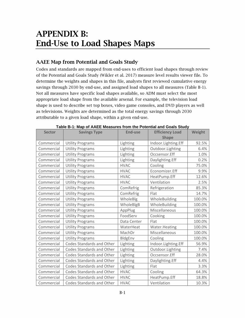
B-1
APPENDIX B: End-Use to Load Shapes Maps
AAEE Map from Potential and Goals Study
Codes and standards are mapped from end-uses to efficient load shapes through review
of the Potential and Goals Study (Wikler et al. 2017) measure level results viewer file. To
determine the weights and shapes in this file, analysts first reviewed cumulative energy
savings through 2030 by end-use, and assigned load shapes to all measures (Table B-1).
Not all measures have specific load shapes available, so ADM must select the most
appropriate load shape from the available arsenal. For example, the television load
shape is used to describe set top boxes, video game consoles, and DVD players as well
as televisions. Weights are determined as the total energy savings through 2030
attributable to a given load shape, within a given end-use.
Table B-1: Map of AAEE Measures from the Potential and Goals Study
Sector Savings Type End-use Efficiency Load Shape
Weight
Commercial Utility Programs Lighting Indoor.Lighting.Eff 92.5%
Commercial Utility Programs Lighting Outdoor.Lighting 6.4%
Commercial Utility Programs Lighting Occsensor.Eff 1.0%
Commercial Utility Programs Lighting Daylighting.Eff 0.2%
Commercial Utility Programs HVAC Cooling 75.0%
Commercial Utility Programs HVAC Economizer.Eff 9.9%
Commercial Utility Programs HVAC HeatPump.Eff 12.6%
Commercial Utility Programs HVAC Ventilation 2.5%
Commercial Utility Programs ComRefrig Refrigeration 85.3%
Commercial Utility Programs ComRefrig Flat 14.7%
Commercial Utility Programs WholeBlg WholeBuilding 100.0%
Commercial Utility Programs WholeBlgB WholeBuilding 100.0%
Commercial Utility Programs AppPlug Miscellaneous 100.0%
Commercial Utility Programs FoodServ Cooking 100.0%
Commercial Utility Programs Data Center Flat 100.0%
Commercial Utility Programs WaterHeat Water.Heating 100.0%
Commercial Utility Programs MachDr Miscellaneous 100.0%
Commercial Utility Programs BldgEnv Cooling 100.0%
Commercial Codes Standards and Other Lighting Indoor.Lighting.Eff 56.9%
Commercial Codes Standards and Other Lighting Outdoor.Lighting 7.4%
Commercial Codes Standards and Other Lighting Occsensor.Eff 28.0%
Commercial Codes Standards and Other Lighting Daylighting.Eff 4.4%
Commercial Codes Standards and Other Lighting Flat 3.3%
Commercial Codes Standards and Other HVAC Cooling 64.3%
Commercial Codes Standards and Other HVAC HeatPump.Eff 18.8%
Commercial Codes Standards and Other HVAC Ventilation 10.3%

B-2
Sector Savings Type End-use Efficiency Load Shape
Weight
Commercial Codes Standards and Other HVAC Flat 6.6%
Commercial Codes Standards and Other ComRefrig Refrigeration 100.0%
Commercial Codes Standards and Other WholeBlg WholeBuilding 100.0%
Commercial Codes Standards and Other WholeBlgB WholeBuilding 100.0%
Commercial Codes Standards and Other AppPlug Miscellaneous 100.0%
Commercial Codes Standards and Other FoodServ Cooking 100.0%
Commercial Codes Standards and Other Data Center Flat 100.0%
Commercial Codes Standards and Other WaterHeat Water.Heating 100.0%
Commercial Codes Standards and Other MachDr Miscellaneous 100.0%
Commercial Codes Standards and Other BldgEnv Cooling 100.0%
Commercial Codes Standards and Other ProcHeat Miscellaneous 100.0%
Residential Utility Programs Lighting ResLighting.Eff 91.6%
Residential Utility Programs Lighting ResOccsensor.Eff 8.4%
Residential Utility Programs AppPlug Dryer 54.7%
Residential Utility Programs AppPlug Refrigerator 43.1%
Residential Utility Programs AppPlug Washer 1.7%
Residential Utility Programs AppPlug Miscellaneous 0.5%
Residential Utility Programs WholeBlg WholeBuilding 100.0%
Residential Utility Programs WholeBlgB WholeBuilding 100.0%
Residential Utility Programs HVAC Cooling.Eff 67.9%
Residential Utility Programs HVAC Heat.Pump.Eff 32.1%
Residential Utility Programs FoodServ Cooking 100.0%
Residential Utility Programs WaterHeat Water.Heating 100.0%
Residential Utility Programs BldgEnv Windows.Eff 41.4%
Residential Utility Programs BldgEnv Insulation.Eff 58.6%
Residential Codes Standards and Other Lighting ResLighting.Eff 100.0%
Residential Codes Standards and Other AppPlug Pool.Pump 49.7%
Residential Codes Standards and Other AppPlug Television 32.5%
Residential Codes Standards and Other AppPlug Miscellaneous 8.9%
Residential Codes Standards and Other AppPlug Refrigerator 7.0%
Residential Codes Standards and Other AppPlug Washer 1.8%
Residential Codes Standards and Other WholeBlg WholeBuilding 100.0%
Residential Codes Standards and Other WholeBlgB WholeBuilding 100.0%
Residential Codes Standards and Other HVAC Cooling.Eff 65.9%
Residential Codes Standards and Other HVAC Heat.Pump.Eff 34.1%
Residential Codes Standards and Other WaterHeat Water.Heating 100.0%
Residential Codes Standards and Other BldgEnv Windows.Eff 100.0%
Residential Codes Standards and Other FoodServ Cooking 100.0%
Map and relative weight of AAEE measures from the Potential and Goals Study.
Source: ADM Associates, Inc.

B-3
Committed Savings
Energy savings from end-uses listed in Committed EE are provided at the utility, sector,
and end-use level. The table below is used to assign load impact profiles to end-uses.
The weights derived specifically for utility sponsored programs from the Potential and
Goals study are applied to committed savings (Table b-2).
Table 15: Map of Committed Savings Measures from the Potential and Goals Study
Sector Committed EE End-use End-use Weight
Agriculture and Water Agricultural WholeBuilding 100.0%
Commercial Building Shell WholeBuilding 100.0%
Commercial CFL Indoor.Lighting.Eff 100.0%
Commercial HVAC (Non-Shell) Cooling 75.0%
Commercial HVAC (Non-Shell) Economizer.Eff 9.9%
Commercial HVAC (Non-Shell) HeatPump.Eff 12.6%
Commercial HVAC (Non-Shell) Ventilation 2.5%
Commercial Lighting (Non-CFL) Indoor.Lighting.Eff 92.5%
Commercial Lighting (Non-CFL) Outdoor.Lighting 6.4%
Commercial Lighting (Non-CFL) Occsensor.Eff 1.0%
Commercial Lighting (Non-CFL) Daylighting.Eff 0.2%
Commercial New Construction WholeBuilding 100.0%
Commercial Other Miscellaneous 100.0%
Commercial Pre-1998 WholeBuilding 100.0%
Commercial Refrigeration Refrigeration 100.0%
Commercial Unspecified Miscellaneous 100.0%
Commercial Water Heating Water.Heating 100.0%
Industrial Industrial WholeBuilding 100.0%
Residential Building Shell WholeBuilding 100.0%
Residential CFL ResLighting.Eff 100.0%
Residential HVAC (Non-Shell) Cooling.Eff 100.0%
Residential Lighting (Non-CFL) ResLighting.Eff 100.0%
Residential New Construction WholeBuilding 100.0%
Residential Other WholeBuilding 100.0%
Residential Pool Pump Pool.Pump 100.0%
Residential Pre-1998 WholeBuilding 100.0%
Residential Refrigeration (Non-Recycling) Refrigerator 100.0%
Residential Refrigerator Recycling Refrigerator 100.0%
Residential Unspecified Miscellaneous 100.0%
Residential Water Heating Water.Heater 100.0%
Map and relative weight of committed savings measures from the Potential and Goals Study.
Source: ADM Associates, Inc.