Calibration of the AASHTOWare Pavement ME Design ...
125
RP 235 Calibration of the AASHTOWare Pavement ME Design Performance Models for Flexible Pavements in Idaho By Fouad Bayomy Ahmed Muftah Emad Kassem University of Idaho Prepared for Idaho Transportation Department Research Program, Contracting Services Division of Engineering Services http://itd.idaho.gov/alt-programs/?target=research-program June 2018 IDAHO TRANSPORTATION DEPARTMENT RESEARCH REPORT
Transcript of Calibration of the AASHTOWare Pavement ME Design ...
RP 235
Calibration of the AASHTOWare Pavement ME
Design Performance Models for Flexible
Pavements in Idaho
By
Fouad Bayomy
Ahmed Muftah
Emad Kassem
University of Idaho
Prepared for
Idaho Transportation Department
Research Program, Contracting Services
Division of Engineering Services
http://itd.idaho.gov/alt-programs/?target=research-program
June 2018
IDA
HO
TR
AN
SPO
RT
AT
ION
DE
PA
RT
ME
NT
RE
SEA
RC
H R
EP
OR
T

Standard Disclaimer
This document is disseminated under the sponsorship of the Idaho Transportation Department and the
United States Department of Transportation in the interest of information exchange. The State of Idaho
and the United States Government assume no liability of its contents or use thereof.
The contents of this report reflect the view of the authors, who are responsible for the facts and
accuracy of the data presented herein. The contents do not necessarily reflect the official policies of the
Idaho Transportation Department or the United States Department of Transportation.
The State of Idaho and the United States Government do not endorse products or manufacturers.
Trademarks or manufacturers’ names appear herein only because they are considered essential to the
object of this document.
This report does not constitute a standard, specification, or regulation.

i
1. Report No.
FHWA-ID-18-235
2. Government Accession No.
3. Recipient’s Catalog No.
4. Title and Subtitle
Calibration of the AASHTOWare Pavement ME Design Performance Models for
Flexible Pavements in Idaho
5. Report Date
June 2018
6. Performing Organization Code
KLK572
7. Author(s)
Fouad Bayomy, Ahmed Muftah, Emad Kassem, Fahmid Tousef, and Hamza Alkuime
8. Performing Organization Report No.
9. Performing Organization Name and Address
University of Idaho
Department of Civil Engineering
875 Perimeter Drive MS 1022
Moscow, ID 83844-1022
10. Work Unit No. (TRAIS)
11. Contract or Grant No.
UI-15-04
12. Sponsoring Agency Name and Address
Idaho Transportation Department (SPR) Division of Highways, Resource Center, Research Program PO Box 7129
Boise, ID 83707-7129
13. Type of Report and Period Covered
Final Report
01/01/2016 - 6/30/2018
14. Sponsoring Agency Code
ITD Report: RP 235
15. Supplementary Notes
Project performed in cooperation with the Idaho Transportation Department and the U.S. Department of Transportation, Federal Highway
Administration.
16. Abstract
This project aims at developing local calibration factors for the AASHTOWare Pavement Mechanistic-Empirical Design (PMED) software. The
performance models included in the software as released by AASHTO are calibrated from national Long-Term Pavement Performance (LTPP)
pavement sites. Hence, the models calibration factors represent averages of national sites across the nation. For specific local conditions, the
performance predicted by the models may deviate from the actual performance observed in the pavements due to varied material, climate,
traffic and site conditions. Therefore, the Idaho Transportation Department (ITD), in its efforts to implement the new AASHTO pavement
design software, launched series of research projects to prepare the required design inputs including materials, traffic and climatic data as
required by the new PMED. To calibrate the software for more accurate perdition of asphalt pavement performance in Idaho, local calibration
of the models was needed. In this project, researchers of the University of Idaho in cooperation with ITD engineers, identified 32 pavement
sites across the state. The sites are selected to represent different geographical, climate and traffic conditions that are mostly prevailing in the
state road network. Structural, material and traffic data for all these pavement sites were accumulated and prepared in accordance to the
PMED software inputs. Actual performance data were collected from ITD Transportation Asset Management System (TAMS) and from ITD
video logs of the selected pavements. The performance predicted by the software was then compared to the actual performance observed in
the field as recorded in TAMS over the pavement service lives. With massive amount of software runs and statistical analysis of the results,
local calibration factors are developed to represent the best case scenario for performance prediction of asphalt pavements in Idaho. The
developed factors were validated using additional nine LTPP sites in Idaho. Furthermore, as part of this project, material testing was
performed to populate the ITD material database with creep compliance and indirect tensile properties at low temperatures that were
missing in the database. An updated and completed ITD database is developed as well. The information in the database is stored in formats
that make it easily accessible and usable by the PMED software.
17. Key Words
Mechanistic-empirical pavement design, asphalt pavements, pavement
performance, local calibration, cracking and rutting.
18. Distribution Statement
Copies available online at http://itd.idaho.gov/alt-
programs/?target=research-program
19. Security Classification (of this report)
Unclassified
20. Security Classification (of this page)
Unclassified
21. No. of Pages
125
22. Price
FHWA Form F 1700.7

ii
METRIC (SI*) CONVERSION FACTORS
APPROXIMATE CONVERSIONS TO SI UNITS APPROXIMATE CONVERSIONS FROM SI UNITS Symbol When You Know Multiply By To Find Symbol Symbol When You Know Multiply By To Find Symbol
LENGTH LENGTH
in inches 25.4 millimeters mm mm millimeters 0.039 inches in
ft Feet 0.3048 meters m m meters 3.28 feet ft
yd yards 0.914 meters m m meters 1.09 yards yd
mi miles (statute) 1.61 kilometers km km kilometers 0.621 Miles (statute) mi
AREA AREA
in2 square inches 645.2 millimeters squared cm2 mm2 millimeters squared 0.0016 square inches in2
ft2 square feet 0.0929 meters squared m2 m2 meters squared 10.764 square feet ft2
yd2 square yards 0.836 meters squared m2 km2 kilometers squared 0.39 square miles mi2
mi2 square miles 2.59 kilometers squared km2 ha hectares (10,000 m2) 2.471 acres ac
ac Acres 0.4046 hectares ha
MASS
(weight)
MASS
(weight)
oz ounces (avdp) 28.35 grams g g grams 0.0353 ounces (avdp) oz
lb pounds (avdp) 0.454 kilograms kg kg kilograms 2.205 pounds (avdp) lb
T short tons (2000 lb) 0.907 megagrams mg mg megagrams (1000 kg) 1.103 short tons T
VOLUME VOLUME
fl oz fluid ounces (US) 29.57 milliliters mL mL milliliters 0.034 fluid ounces (US) fl oz
gal Gallons (liq) 3.785 liters liters liters liters 0.264 Gallons (liq) gal
ft3 cubic feet 0.0283 meters cubed m3 m3 meters cubed 35.315 cubic feet ft3
yd3 cubic yards 0.765 meters cubed m3 m3 meters cubed 1.308 cubic yards yd3
Note: Volumes greater than 1000 L shall be shown in m3
TEMPERATURE
(exact)
TEMPERATURE
(exact)
oF Fahrenheit
temperature
5/9 (oF-32) Celsius
temperature
oC oC Celsius temperature 9/5 oC+32 Fahrenheit
temperature
oF
ILLUMINATION ILLUMINATION
fc foot-candles 10.76 lux lx lx lux 0.0929 foot-candles fc
fl foot-lamberts 3.426 candela/m2 cd/cm2 cd/cm2
candela/m2 0.2919 foot-lamberts fl
FORCE and
PRESSURE or
STRESS
FORCE and
PRESSURE or
STRESS
lbf pound-force 4.45 newtons N N newtons 0.225 pound-force lbf
psi pound-force per
square inch
6.89 kilopascals kPa kPa kilopascals 0.145 pound-force per
square inch
psi
iii
Acknowledgements
This project is funded by Idaho Transportation Department (ITD) from SPR funds. It is performed in
cooperation with ITD. The authors would like to acknowledge all members of the research project
Technical Advisory Committee (TAC) for their valuable feedback and cooperation all over the project
tasks. The authors would like to thank many professionals at ITD for their technical help and feedback.
The authors also would like to acknowledge the work and support of many individuals at the University
of Idaho who participated in the completion of this project. Graduate students Hamza Alkuime, Fahmid
Tousif and Mumtahin Hasnat worked on the laboratory testing of creep compliance and Indirect Tension
tests, Video Logs data analysis and the development of the performance database. Their efforts are
acknowledged and greatly appreciated. The authors also acknowledge and appreciate all the support
provided by the administrative staff at the National Institute of Advanced Transportation Technology
(NIATT) at the University of Idaho.
The cooperation and support provided by the Washington State University (WSU) is also acknowledged.
Major part of Task 4 (Development of Creep Compliance Data) was performed at WSU by Mr. Amir
Bahadori, a graduate student, under the supervision of Professor Haifang Win. Their cooperation and
timely delivery is greatly appreciated.
At last, but not least, special thanks are due to Dr. Linda Pierce for her critical review and invaluable
suggestions and feedback. Dr. Pierce not only served as the peer reviewer of the report, but also
contributed significantly to the technical editing of the report. The authors greatly appreciate her efforts
and timely review.
Technical Advisory Committee
Each research project is overseen by a technical advisory committee (TAC), which is led by an ITD project
sponsor and project manager. The Technical Advisory Committee (TAC) is responsible for monitoring
project progress, reviewing deliverables, ensuring that study objective are met, and facilitating
implementation of research recommendations, as appropriate. ITD’s Research Program Manager
appreciates the work of the following TAC members in guiding this research study.
Project Sponsor – John Bilderback, P.E.
Project Manager – Mike Santi, P.E.
TAC Members
John Arambarri, P.E. Chad Clawson, P.E. James Poorbaugh, P.E. Mark Wheeler, P.E.
FHWA-Idaho Advisor – Kyle Holman, P.E.

iv

v
Table of Contents
Executive Summary .....................................................................................................................................xiii
Introduction ...............................................................................................................................................xiii
Research Methodology..............................................................................................................................xiii
Key Findings ...............................................................................................................................................xiii
Recommendations ..................................................................................................................................... xiv
Chapter 1 Introduction................................................................................................................................. 1
Background .................................................................................................................................................. 1
Problem Statement ..................................................................................................................................... 1
Scope of Research and Project Tasks .......................................................................................................... 2
Report Organization .................................................................................................................................... 4
Chapter 2 Review of the PMED Distress Prediction Models for Flexible Pavements .................................. 7
Performance Indicators ............................................................................................................................... 7
Alligator Cracking (Bottom-Up Cracking) .............................................................................................. 7
Longitudinal Cracking (Top-down Cracking) ......................................................................................... 7
Thermal Transverse Cracking ................................................................................................................ 7
Transverse Reflection Cracking ............................................................................................................. 8
Rutting ................................................................................................................................................... 8
International Roughness Index (IRI) ...................................................................................................... 8
Performance Models in the PMED Software............................................................................................... 8
AC Rutting Prediction Model ................................................................................................................ 9
Rutting Prediction Model for Unbound Materials and Subgrade Soil ................................................ 10
Load Associated Cracking Prediction Models ..................................................................................... 12
Non-Load Associated Transverse Cracking Prediction Model ............................................................ 17
Reflection Cracking in AC Overlays ..................................................................................................... 18
Smoothness Prediction Model ............................................................................................................ 19
PMED Calibration and Implementation Efforts by State DOTs ................................................................. 20
Arizona ................................................................................................................................................ 21
California ............................................................................................................................................. 22
Montana .............................................................................................................................................. 22
Nevada ................................................................................................................................................ 23
Oregon ................................................................................................................................................ 23
Utah ..................................................................................................................................................... 24

vi
Washington ......................................................................................................................................... 25
Wyoming ............................................................................................................................................. 26
State DOT PMED Implementation Summary ............................................................................................. 27
Chapter 3 Development of PMED Calibration Coefficients for Idaho ........................................................ 33
Procedures of the MEPDG Guide for Local Calibration ............................................................................. 34
Idaho Local Calibration Procedures ........................................................................................................... 36
Hierarchical Input Level Selection for Each Input Parameter ............................................................. 36
Develop Local Experimental Plan and Sampling Template (Matrix) ................................................... 44
Estimate Sample Size for Specific Distress Prediction Models ........................................................... 45
Roadway Segments Selection ............................................................................................................. 47
Extract and Evaluate Distress Project Data ......................................................................................... 50
Conduct Field and Forensic Investigations ......................................................................................... 54
Assess Local Bias: Validation of Global Calibration Values to Local Conditions, Polices, and Materials ............................................................................................................................................................ 56
Eliminate Local Bias of Distress and IRI Prediction Models ................................................................ 58
Assess the Standard Error of the Estimate ......................................................................................... 58
Reduce Standard Error of the Estimate .............................................................................................. 59
Results of Calibration of Performance Models ......................................................................................... 59
Rutting Models .................................................................................................................................... 59
Longitudinal (Top-Down) Cracking Model .......................................................................................... 64
Alligator (Bottom-Up) Cracking Model ............................................................................................... 65
Thermal (Transverse) Cracking Model ................................................................................................ 65
International Roughness Index Model ................................................................................................ 65
Chapter 4 Validation of the Developed Calibration Coefficients ................................................................ 69
Chapter 5 Summary, Conclusions, and Recommendations ........................................................................ 77
Summary .................................................................................................................................................... 77
Conclusions ................................................................................................................................................ 78
Recommendations ..................................................................................................................................... 79
References .................................................................................................................................................. 81
Appendix A Updated PMED Database to Include Creep Compliance and IDT Data (e-file) ....................... 85
Appendix B Performance Database .......................................................................................................... 105
vii
List of Tables
Table 1 Arizona Local Calibration Coefficients(14) ........................................................................................ 22
Table 2 Montana Local Calibration Coefficients(16) ..................................................................................... 23
Table 3 Oregon Local Calibration Coefficients(21) ........................................................................................ 24
Table 4 Utah Local Calibration Coefficients(22) ............................................................................................ 25
Table 5 Washington State Local Calibration Coefficients (23) ...................................................................... 26
Table 6 Wyoming Local Calibration Coefficients(6) ...................................................................................... 27
Table 7 Summary of Local Calibration Coefficients for Rutting ................................................................. 28
Table 8 Summary of Calibration Coefficients for Fatigue Cracking ........................................................... 29
Table 9 Summary of Local Calibration Coefficients for Transverse Cracking.............................................. 30
Table 10 Summary of Local Calibration Coefficients for IRI ........................................................................ 31
Table 11 Required Flexible Pavement Input Parameters(3,5) ....................................................................... 37
Table 12 Example of Sensitivity Analysis Effective Binder Content and Distress Prediction ...................... 39
Table 13 Summary of Very Significant to Significant Key Design Input Parameters for New Flexible
Pavements(4) ................................................................................................................................................ 40
Table 14 Summary of Received Field Cores Based on Mix Type and Asphalt Binder ................................. 43
Table 15 Creep Compliance Test Results for Mix (KN13823),(1/psi) .......................................................... 44
Table 16 IDT Test Results for Mix (KN13823),(psi)...................................................................................... 44
Table 17 Local Experimental Plan and Sampling Template ........................................................................ 45
Table 18 Minimum Recommended Number of Pavement Sections for Local Calibration ......................... 47
Table 19 List of the Roadway Segments Selected for Local Calibration ..................................................... 48
Table 20 Asphalt and Rigid Pavement Cracking Types Collected in Idaho ................................................. 50
Table 21 Comparison between ITD and PMED Flexible Pavement Distresses ........................................... 51
Table 22 Cracks Types, Extent, and Severity Level ..................................................................................... 52
Table 23 Summary of Statistical Analysis of Predicted vs. Measured Distress Using the Global Calibration
Coefficients ................................................................................................................................................. 57
Table 24 Calibration Parameters to Adjust to Eliminate Bias(3,5) ................................................................ 58
Table 25 Calibration Parameters to Adjust to Reduce the Standard Error(3,5) ............................................ 59
Table 26 Calibration Coefficients for AC Layer Rutting ............................................................................... 60
viii
Table 27 Calibration Coefficients for Base Layer Rutting............................................................................ 61
Table 28 Calibration Coefficients for Subgrade Rutting.............................................................................. 62
Table 29 Calibration Coefficients for Rutting .............................................................................................. 63
Table 30 Calibration Coefficients for Longitudinal Cracking ....................................................................... 65
Table 31 Calibration Coefficients for Alligator Cracking ............................................................................. 66
Table 32 Calibration Coefficients for Thermal Cracking ............................................................................. 67
Table 33 Calibration Coefficients for IRI ..................................................................................................... 68
Table 34 Local Calibration Coefficients for AC Rutting ............................................................................... 70
Table 35 Local Calibration Coefficients for Base Layer Rutting .................................................................. 71
Table 36 Local Calibration Coefficients for Subgrade Rutting .................................................................... 71
Table 37 Local Calibration Coefficients for Total Rutting ........................................................................... 72
Table 38 Local Calibration Coefficients for Alligator Cracking .................................................................... 73
Table 39 Local Calibration Coefficients for Longitudinal Cracking .............................................................. 73
Table 40 Local Calibration Coefficients for Thermal Cracking .................................................................... 74
Table 41 Calibration Coefficients for IRI ..................................................................................................... 75
Table 42 Summary of Calibration Coefficients Before and After Local Calibration .................................... 77

ix
List of Figures
Figure 1 AC Rutting Prediction Model .......................................................................................................... 9
Figure 2 Rutting Prediction Equations for Unbound Materials and Subgrade Soil ..................................... 10
Figure 3 Comparison of Measured and Predicted Total Rutting Resulting from Global Calibration (11) ..... 11
Figure 4 Standard Error Equations for the Rutting Models ........................................................................ 11
Figure 5 PMED Equations for the Allowable Number of Traffic Repetitions to Fatigue Damage............... 12
Figure 6 PMED Equation for the Damage Ratio .......................................................................................... 13
Figure 7 Bottom-Up Cracking Transfer Function ........................................................................................ 13
Figure 8 Comparison of Cumulative Fatigue Damage and Measured Alligator Cracking Resulting from
Global Calibration Process (11) ..................................................................................................................... 14
Figure 9 Comparison of Cumulative Fatigue Damage and Measured Alligator Cracking Resulting from
Global Calibration Process (11) ..................................................................................................................... 14
Figure 10 Top-Down Transfer Function ...................................................................................................... 15
Figure 11 Standard Error Equations for Bottom-Up and Top-Down Cracking ............................................ 15
Figure 12 Fatigue Cracking Prediction Model for CTB Layers ..................................................................... 16
Figure 13 CTB Layer Damaged Modulus Equation ...................................................................................... 17
Figure 14 PMED Thermal Cracking Model .................................................................................................. 17
Figure 15 Standard Error Equations for the Thermal Cracking ................................................................... 17
Figure 16 Paris Law for Crack Propagation ................................................................................................. 18
Figure 17 Reflection Cracking Model in AC Overlays .................................................................................. 19
Figure 18 Smoothness Prediction Model .................................................................................................... 20
Figure 19 Summary of Agency PMED Implementation(12) .......................................................................... 21
Figure 20 Target Analogy for Precision and Accuracy(32) ............................................................................ 33
Figure 21 Improvement of Bias and Precision through Local Calibration(34) .............................................. 34
Figure 22 Summary of Sensitivity Analysis and Input Effect on Rutting ..................................................... 40
Figure 23 Example of Road Segment Input Data ........................................................................................ 42
Figure 24 Estimation of Minimum Sample Size .......................................................................................... 46
Figure 25 Geographical Locations of the Selected Road Segments for Local Calibration .......................... 49
Figure 26 Example of Extracted Images of the Video-Based Distress Data Collection ............................... 53

x
Figure 27 Example of Data Sheet for Cracking Analysis Using PathView Video Images ............................. 54
Figure 28 Plan of SH008 Trench Locations .................................................................................................. 55
Figure 29 Trench Side View ......................................................................................................................... 55
Figure 30 Example of Trench Rut Depth Measurements on SH008 ........................................................... 56
Figure 31 Distress Indictors (Rutting and IRI) with the Null Hypothesis Test ............................................. 57
Figure 32 Measured vs. Predicted AC Rutting Using Global Calibration Coefficients ................................ 60
Figure 33 Measured vs. Predicted AC Rutting Using Local Calibration Coefficients ................................... 60
Figure 34 Measured vs. Predicted Granular Base Rutting Using Global Calibration Coefficients .............. 61
Figure 35 Measured vs. Predicted Granular Base Rutting Using Local Calibration Coefficients ................ 61
Figure 36 Measured vs. Predicted Subgrade Rutting Using Global Calibration Coefficients ...................... 62
Figure 37 Measured vs. Predicted Subgrade Rutting Using Local Calibration Coefficients ........................ 62
Figure 38 Measured vs. Predicted Total Rutting Using Global Calibration Coefficients ............................. 63
Figure 39 Measured vs. Predicted Total Rutting Using Local Calibration Coefficients ............................... 63
Figure 40 Measured vs. Predicted Longitudinal Cracking Using Global Calibration Coefficients ............... 64
Figure 41 Measured vs. Predicted Longitudinal Cracking Using Local Calibration Coefficients ................. 64
Figure 42 Measured vs. Predicted Alligator Cracking Using Global Calibration Coefficients ..................... 66
Figure 43 Measured vs. Predicted Alligator Cracking Using Local Calibration Coefficients ....................... 66
Figure 44 Measured vs. Predicted Transverse Cracking Using Global Calibration Coefficients ................. 67
Figure 45 Measured vs. Predicted Transverse Cracking Using Local Calibration Coefficients ................... 67
Figure 46 Measured vs. Predicted IRI Using Global Calibration Coefficients ............................................. 68
Figure 47 Measured vs. Predicted IRI using Local Calibration Coefficients ................................................ 68
Figure 48 Measured vs. Predicted AC Using Local Calibration Coefficients ............................................... 70
Figure 49 Measured vs. Predicted Base Layer Rutting Using Local Calibration Coefficients ...................... 70
Figure 50 Measured vs. Predicted Subbase Layer Rutting Using Local Calibration Coefficients ................ 71
Figure 51 Measured vs. Predicted Total Rutting Using Local Calibration Coefficients ............................... 72
Figure 52 Measured vs. Predicted Alligator Cracking Using Local Calibration Coefficients ....................... 72
Figure 53 Measured vs. Predicted Longitudinal Cracking Using Local Calibration Coefficients ................. 73
Figure 54 Measured vs. Predicted Thermal Cracking Using Local Calibration Coefficients ........................ 74
Figure 55 Measured vs. Predicted IRI Using Local Calibration Coefficients ................................................ 74

xi
List of Acronyms
AADT Annual average daily traffic
AADTT Annual average daily truck traffic
AASHO American Association of State Highway Officials
AASHTO
American Association of State Highway and Transportation Officials
AC Asphalt concrete
CBR California Bearing Ratio CBR
CC Creep compliance
CI Cracking Index
DOT Department of Transportation
E* Dynamic Modulus
EICM Enhanced integrated climatic model
ESAL Equivalent single axle load
FHWA Federal Highway Agency
HMA
Hot mix asphalt
IDT
Indirect tensile test
ITD
Idaho Transportation Department
IRI International Roughness Index
JMF Job mix formula
JPCP Jointed plain concrete pavement
LTPP Long Term Pavement Performance
MAF Monthly adjustment factor
ME Mechanistic-empirical
MEPDG
Mechanistic-Empirical Pavement Design Guide
MR Resilient modulus
NCHRP National Cooperative Highway Research Program
NMAS
Nominal maximum aggregate size
PG
Performance grade
PMED AASHTOWare Pavement ME Design™ software
PPMIS ITD Pavement Performance Management Information System
Se Standard Error
SP-# Superpave Mix-#
TAMS Transportation Asset Management System
VCD Vehicle class distribution
VFA
Voids filled with asphalt
VMA
Voids in mineral aggregate
WIM Weigh-in-motion

xii
Executive Summary
xiii
Executive Summary
Introduction
This report summarizes findings from research conducted for the Idaho Transportation Department
(ITD). The study objective included developing a detailed, statistically sound, and practical experimental
plan for validating, and potentially calibrating, the AASHTOWare Pavement ME Design™ (PMED) asphalt
pavement performance models to Idaho conditions. The validation and calibration process involved
laboratory testing to determine the asphalt Concrete materials properties, conducting PMED analysis
based on globally-calibrated performance prediction models, and comparing the results to local
performance observations. A statistical comparison of results indicated the PMED asphalt pavement
performance models, using the global calibration coefficients, did not reflect Idaho conditions.
Therefore, recalibration was recommended and local calibration coefficients were determined.
Research Methodology
The PMED is a comprehensive tool for the analysis and design of new and rehabilitated flexible and rigid
pavement structures based on mechanisticempirical (ME) principles. The PMED pavement performance
prediction models are based on globally-calibrated models and may not necessarily reflect pavement
performance in Idaho. Therefore, it is essential to evaluate, validate, and if necessary calibrate, the
PMED pavement performance prediction models to local conditions. In 2009, ITD initiated a major effort
toward the implementation of the PMED. The main focus of the implementation was to establish a
comprehensive material, traffic, and climatic input database. Under a separate study, an
implementation plan and design guide to help ITD personnel with implementing the PMED was
developed. The research effort discussed in this report is the last phase toward successful
implementation of the PMED based on Idaho conditions. The calibration and validation of the
performance models was conducted per the American Association of State Highway and Transportation
Officials (AASHTO) Guide for the Local Calibration of the Mechanistic-Empirical Pavement Design Guide(3)
and the Road Map for Implementing The AASHTO Pavement ME Design Software for the Idaho
Transportation Department, ITD project RP211A.(5)
Key Findings
The globally-calibrated PMED rutting model overestimates the total (accumulated) rutting as
compared to field-measured values. The rutting model was locally-calibrated to improve the
prediction, with less bias and errors.
The globally-calibrated alligator (bottom-up) cracking model provides reasonable predictions for
Idaho conditions.

Calibration of the AASHTOWare Pavement ME Design Performance Models for Flexible Pavements in Idaho
xiv
The globally-calibrated longitudinal (top-down) cracking model provides poor predictions with high
bias and standard error. The locally-calibrated coefficients reduced the bias and the error; however,
there is still a statistically significant difference between the observed and predicted cracking. Many
studies recommend that the longitudinal cracking model should only be used for
experimental/informational purposes, the longitudinal cracking model is currently undergoing
refinement as part of National Highway Research Cooperative (NCHRP) Project 1-52, A Mechanistic-
Empirical Model for Top-Down Cracking of Asphalt Pavement Layers.
The globally-calibrated thermal cracking model under predicts thermal cracking as compared to
field-measured values. Therefore, the thermal cracking model was calibrated, and the results
showed significant improvement in the model prediction with less bias and error.
The reflective cracking model was not calibrated due to lack of data on field-measured reflective
cracking.
The semi-rigid fatigue cracking model was not calibrated in this study. All pavement sections
selected for the calibration effort excluded AC over jointed plain concrete pavement (JPCP) sections.
Also, for sections with cement treated base, there was no field-observed fatigue cracking. For these
reasons, the research team was unable to calibrate the semi-rigid fatigue cracking model.
Recommendations
The calibration of the PMED pavement performance prediction models is a continual process. The
local calibration effort should result in models with reasonable bias between predicted and
observed models. As additional years of performance data are obtained, and as new models are
added and existing models are revised, recalibration may be warranted.
Ongoing and future work that examines and assesses PMED pavement performance prediction
models and software updates should continue to be monitored. The pavement performance
database developed in this study provides the needed data to evaluate future PMED performance
prediction model updates.
At this time, the PMED longitudinal (top-down) cracking model should only be used for experimental
or informational purposes.
Some of the challenges identified in this study were the lack of observed pavement distress, limited
range of distress values, and shorter pavement service life. Therefore, the research team
recommends monitoring the sections used in the calibration effort until the next major
rehabilitation project.
ITD, through preventive maintenance, applies seal coats on many major pavement sections. The seal
coat application limits the observation of distresses in the field, which may lead to an inaccurate

Executive Summary
xv
assessment of pavement performance on these sections. Thus, pavement sections with seal coats
should be excluded from use with future calibration efforts.
One of the future tools that may be provided in the PMED software is automation of the local
calibration process. The local calibration tool will require a database that contains sections with
pavement performance information. Emphasizing the importance of the developed database and
the vital role it will play in providing accurate and precise data for the performance of the flexible
pavements under Idaho conditions. Therefore, continual population and maintenance of the
performance database is strongly recommended.

Calibration of the AASHTOWare Pavement ME Design Performance Models for Flexible Pavements in Idaho
xvi

Chapter 1: Introduction
1
Chapter 1
Introduction
Background
The American Association of State Highway Officials (AASHO) developed its first pavement design guide
in 1961.(1) The guide was a result of experiments at the AASHO test road during the 1950-1960s. This
empirical-based design method had a number of limitations, including a single climatic region (Ottawa,
Illinois), limited traffic loads (vehicle type and weight), as well as, a limited range of materials (e.g., one
asphalt binder type, one base type, one subgrade soil type). With advancements in material
characterization and pavement performance evaluation, the American Association of State Highway and
Transportation Officials (AASHTO) developed the Mechanical Empirical Pavement Design Guide, A
Manual of Practice (MEPDG), and accompanying software, through the National Cooperative Highway
Research Program (NCHRP) Project 01-37A, Development of the 2002 Guide for the Design of New and
Rehabilitated Pavement Structures: Phase II.(2) The accompanying software has received multiple
updates and revisions and is now available as AASHTOWare Pavement ME Design™ (PMED).
In the mechanistic-empirical (ME) design process, cumulative pavement distresses are calculated based
on pavement response (e.g., stress, strain, deflection) and empirical distress performance models that
relate pavement response to observed distress. Various distresses can be predicted, such as, rutting in
each layer, bottom-up and top-down cracking, reflective cracking, thermal cracking, and roughness
(characterized by the International Roughness Index [IRI]). The performance models used in the PMED
were globally-calibrated using data obtained from in-service pavements, primarily from the Long Term
Pavement Performance (LTPP) program.
Accordingly, the globally-calibrated models should be evaluated to determine whether they accurately
predict field performance, if not, the models should be calibrated to local conditions. Otherwise, some
pavements may be overdesigned and others under designed, resulting in either excessive costs or
shortened pavement life. AASHTO highly recommends that each agency conduct an analysis of the
PMED results to determine if the globally-calibrated performance models accurately predict field
performance.(3)
Problem Statement
The Idaho Transportation Department (ITD) maintains more than 12,200 lane-miles of roads. With a
large roadway system and a limited budget, it is essential that proper pavement structures are designed
and constructed to withstand anticipated traffic loads and climate conditions over the intended design
life. In 2010, ITD developed a plan to assist with the implementation of the PMED.(4,5,6) The
implementation plan included developing traffic inputs, characterizing material properties for asphalt
mixes, unbound aggregate layers, and subgrade soils. In addition, a user’s guide was developed to assist

Calibration of the AASHTOWare Pavement ME Design Performance Models for Flexible Pavements in Idaho
2
ITD personnel with the implementation of the PMED. One of the final steps for PMED implementation
includes validating, and if needed, locally calibrating the PMED pavement performance models.
Scope of Research and Project Tasks
The scope of this project includes developing the local calibration coefficients for asphalt pavement
performance models specific to Idaho conditions. This project was divided into the following tasks:
Task 1: Review the PMED pavement performance prediction models for flexible pavements. The
distress and IRI prediction models, as well as the global calibration coefficients, shall be
reviewed. Trial runs will be performed with the most current PMED version.
Task 2: Evaluate the required PMED design inputs. In this task, the research team will study and
evaluate the inputs required to run the latest PMED version. In addition, the level of input for
each required parameter will be determined based on previous literature studies, as well as ITD
available data.
Task 3: Identify and select the pavement sections for calibration. In addition to the LTPP projects
available in Idaho, the research team, in coordination with ITD, will identify and select roadway
sections representative of the different districts in Idaho. The pavement sections shall cover a
reasonable range of climate conditions, traffic levels, and subgrade strength. The selected
pavement sections shall have all required PMED inputs and sufficient field-measured
performance data (both to be provided by ITD). Requested data includes, but not limited to:
Project location (latitude and longitude).
Construction year and month.
As-built pavement structure (layer type and thickness of each layer).
AC, base, subbase, and subgrade material properties.
Ground water table level.
Traffic volume and axle load spectra data in the required PMED format.
Performance data (rutting, longitudinal cracking, alligator fatigue cracking, transverse
cracking, and IRI) since original construction.
Maintenance history.
Based on the research teams experience with ITD data for in-service pavement sections, level 1
input data will be difficult to obtain for most of the required inputs. Therefore, level 2 and 3
input data will be used when level 1 data is unavailable. Previous outcomes of ITD Project RP
193 (KLK557), Implementation of the MEPDG for Flexible Pavements in Idaho, will play a vital
role in the characterization of the material, traffic, and climate of the selected pavement
sections.
Chapter 1: Introduction
3
Selected pavement sections should have in-service lives of more than 5 years. Pavement
sections close to receiving major rehabilitation activities are preferred since their condition
tends to include a variety of distress types and severities. Selected pavement sections also need
to include Superpave asphalt mixes to utilize the materials database developed under RP 193.
The total number of required pavement sections, including the Idaho LTPP flexible pavement
sections, will be determined by the research team in coordination with ITD.
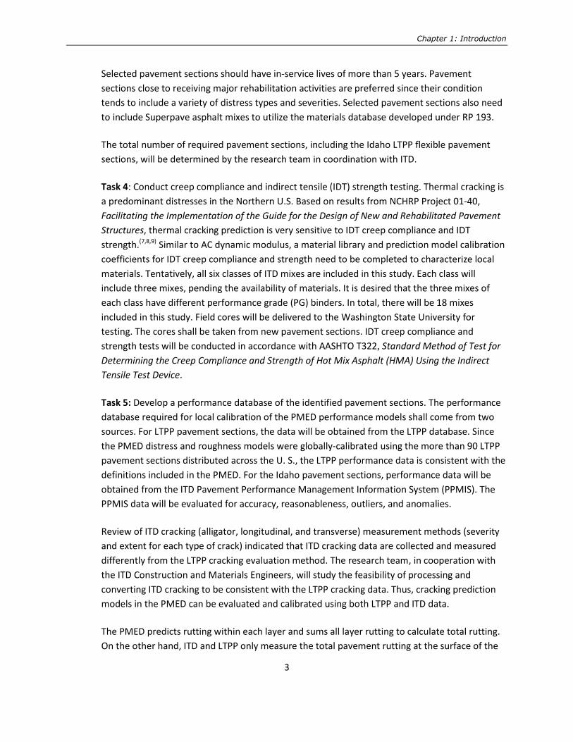
Task 4: Conduct creep compliance and indirect tensile (IDT) strength testing. Thermal cracking is
a predominant distresses in the Northern U.S. Based on results from NCHRP Project 01-40,
Facilitating the Implementation of the Guide for the Design of New and Rehabilitated Pavement
Structures, thermal cracking prediction is very sensitive to IDT creep compliance and IDT
strength.(7,8,9) Similar to AC dynamic modulus, a material library and prediction model calibration
coefficients for IDT creep compliance and strength need to be completed to characterize local
materials. Tentatively, all six classes of ITD mixes are included in this study. Each class will
include three mixes, pending the availability of materials. It is desired that the three mixes of
each class have different performance grade (PG) binders. In total, there will be 18 mixes
included in this study. Field cores will be delivered to the Washington State University for
testing. The cores shall be taken from new pavement sections. IDT creep compliance and
strength tests will be conducted in accordance with AASHTO T322, Standard Method of Test for
Determining the Creep Compliance and Strength of Hot Mix Asphalt (HMA) Using the Indirect
Tensile Test Device.
Task 5: Develop a performance database of the identified pavement sections. The performance
database required for local calibration of the PMED performance models shall come from two
sources. For LTPP pavement sections, the data will be obtained from the LTPP database. Since
the PMED distress and roughness models were globally-calibrated using the more than 90 LTPP
pavement sections distributed across the U. S., the LTPP performance data is consistent with the
definitions included in the PMED. For the Idaho pavement sections, performance data will be
obtained from the ITD Pavement Performance Management Information System (PPMIS). The
PPMIS data will be evaluated for accuracy, reasonableness, outliers, and anomalies.
Review of ITD cracking (alligator, longitudinal, and transverse) measurement methods (severity
and extent for each type of crack) indicated that ITD cracking data are collected and measured
differently from the LTPP cracking evaluation method. The research team, in cooperation with
the ITD Construction and Materials Engineers, will study the feasibility of processing and
converting ITD cracking to be consistent with the LTPP cracking data. Thus, cracking prediction
models in the PMED can be evaluated and calibrated using both LTPP and ITD data.
The PMED predicts rutting within each layer and sums all layer rutting to calculate total rutting.
On the other hand, ITD and LTPP only measure the total pavement rutting at the surface of the
Calibration of the AASHTOWare Pavement ME Design Performance Models for Flexible Pavements in Idaho
4
asphalt concrete (AC) layer. Thus, for rutting model calibration, the focus will be on total rut-
depth. Percentages of the sub-layer rutting, based on engineering reasonableness, as well as the
globally-calibrated rutting models will be assumed.
Task 6: Run the PMED using the globally-calibrated models with the developed database. The
PMED will be run and the predicted performance compared to the field-measured performance.
Precision and bias of the globally-calibrated performance models will be assessed. This will
warrant whether or not the globally-calibrated models need to be locally calibrated.
Task 7: Develop Idaho calibration coefficients. In this task, using the outcomes of Task 5, the
PMED will be run using different trial sets of calibration coefficients for each performance model
to determine the best combination of calibration coefficients. The set of local calibration
coefficients that produce a higher precision and lower bias for each distress model, as compared
to the globally-calibrated models, will be selected. The IRI model will be calibrated after the
distress models since it is dependent on the predicted rutting and cracking, as well as other
factors. Finally, the resulting goodness of fit and bias of the locally-calibrated models will be
statistically validated.
Task 8: Summary of findings and recommendations. Before completing the final report and
developing the training workshop, a summary of findings and draft calibration coefficients will
be developed and submitted to ITD for review. ITD review comments and recommendations will
be incorporated in the final report and the training workshop.
Task 9: Prepare and conduct training workshop. The IDT PMED User Manual will be reviewed
and updated to reflect the new findings from this project. A workshop to demonstrate and train
ITD personnel on the new software will be performed at a suitable location where access to the
software will be available.
Task 10: Final report. A draft report will be edited by a professional editor and reviewed by an
external expert. The edited and reviewed draft report will be submitted to ITD for comments
before submission of the final report.
Report Organization
This report presents the research work completed for the validation and calibration of the PMED to
Idaho conditions. The report is organized into five chapters as described below:
Chapter 1 provides the introduction of this research project, presents the problem statement,
research objectives, and project description.

Chapter 1: Introduction
5
Chapter 2 presents a literature review of the PMED pavement performance prediction models
for flexible pavements, and summarizes other State Department of Transportation (DOT) PMED
implementation efforts.
Chapter 3 presents the local calibration process, results, and analysis of the development of
Idaho-specific local calibration coefficients.
Chapter 4 presents the validation process of the determined local calibration coefficients to
Idaho conditions.
Finally, Chapter 5 summarizes the key findings from this research and presents
recommendations for future work for ITD consideration.

Calibration of the AASHTOWare Pavement ME Design Performance Models for Flexible Pavements in Idaho
6

Chapter 2: Review of the PMED Distress Prediction Models for Flexible Pavements
7
Chapter 2
Review of the PMED Distress Prediction Models for Flexible
Pavements
This chapter presents a summary of the asphalt pavement performance prediction models included in
the PMED and a review of PMED implementation efforts conducted by other state DOTs. The purpose of
the state DOT review is to learn what activities need to be performed to overcome the challenges with
local calibration and successful implementation of the PMED. Summary of the implementation plans of
the surrounding agencies, and their developed local calibration coefficients is also presented below.
Performance Indicators
PMED analyzes pavement’ performance over its design life. Pavement distress is determined using
transfer functions and structural response models. The response models compute critical pavement
stresses, strains, and deflections through mechanistic models and empirical transfer functions relate
these critical pavement responses to performance indicators. The following discusses each of the
distress models within the PMED.
Alligator Cracking (Bottom-Up Cracking)
Alligator cracking develops through repeated wheel loading and is defined as a series of interconnected
cracks due to AC fatigue or stabilized base (characteristically with an “alligator hide” pattern). Alligator
cracks initiate at the bottom of the AC layer and propagate to the surface. They initially show up as
multiple short, longitudinal, or transverse cracks in the wheel path, becoming interconnected with
continued truck loading. Alligator cracking is calculated as a percent of total lane area.(10,11)
Longitudinal Cracking (Top-down Cracking)
Longitudinal cracking is a load-related distress, occurring within the wheel paths, that primarily runs
parallel to the pavement centerline. Longitudinal cracking initiates at the surface of the AC layer due to
high localized tensile stresses from tire-pavement interaction.(11) Longitudinal cracking initially shows up
as short cracks that become connected with continued truck loadings. Raveling or crack deterioration
may occur along the edges of these cracks but they do not form an alligator cracking pattern. The PMED
calculates longitudinal cracking as total feet per mile (includes both wheel paths).(11)
Thermal Transverse Cracking
Thermal (transverse) cracking is non-wheel load-related cracking that appears perpendicular to the
pavement centerline and is caused by low temperatures. The PMED calculates transverse cracking as
total feet per mile.
Calibration of the AASHTOWare Pavement ME Design Performance Models for Flexible Pavements in Idaho
8
Transverse Reflection Cracking
Transverse reflection cracking is a non-wheel load crack that is induced by transverse joints or cracks in
the underlying pavement. Transverse reflection cracking is calculated in the PMED as the percent lane
area (area cracked = linear ft of crack × 1 ft width, where crack width = 1 ft).(11)
Rutting
Rutting is a surface depression in the wheel path caused by plastic or permanent deformation in each
pavement layer. The rut depth represents the maximum vertical difference in elevation between the
transverse profile of the pavement surface and a wire-line across the lane width. The PMED calculates
rut depth in inches, and represents the maximum mean rut depth in both wheel paths. The PMED
calculates total rutting and rutting in each pavement layer (AC, unbound aggregate layers, and
subgrade).(11)
International Roughness Index (IRI)
The PMED predicts the incremental change in smoothness over the entire design period. The IRI model
uses the predicted distresses (rutting, bottom-up/top-down fatigue cracking, and thermal cracking),
initial IRI, subgrade condition, site factors, and climatic factors to predict IRI over the design period.
Performance Models in the PMED Software
The PMED predicts pavement distress by dividing the pavement structural layers into thinner sublayers.
The thickness of the sublayers depends upon the layer thickness, layer type, and depth within the
pavement structure. The JULEA program calculates the critical responses (stress and strain) in each
sublayer.(2) For load related distresses, the AC dynamic modulus (E*) is calculated as a function of time
at mid-depth of the AC layer. This is done by dividing the hourly temperatures of the AC sublayers over a
given analysis period (2 weeks to 1 month) into five sub-seasons For each sub-season, the temperature
of AC sublayer represents 20 percent of the pavement temperature distribution frequency. This sub-
season similarly represents these conditions when 20 percent of the monthly traffic takes place. This is
done by computing pavement temperatures corresponding to standard normal deviations of -1.2816,
-0.5244, 0, 0.5244 and 1.2816. These values correspond to accumulated frequencies of 10, 30, 50, 70
and 90 percent within a given month. The software uses these five quintile temperatures to calculate
the dynamic modulus (E*) at the mid-depth of each AC sublayer taking into account the effect of loading
rate (vehicle speed) and temperature variation through the analysis period. E* is used for permanent
deformation and fatigue damage calculations.(2,4) For transverse cracking, the Enhanced Integrated
Climatic Model (EICM) processes the AC temperatures on an hourly basis. The hourly temperatures are
used to predict AC creep compliance and IDT strength to compute the tensile strength of the surface AC
layer. The following sections present the computational steps used in the PMED to estimate distress,
and the local calibration coefficients that need to be determined for each distress prediction model.
(2,4,10,11)

Chapter 2: Review of the PMED Distress Prediction Models for Flexible Pavements
9
AC Rutting Prediction Model
PMED uses two different models to predict rutting, one for AC layers, and the other for unbound base
and subgrade layers. The model for the AC layer is shown below.
∆𝒑(𝑨𝑪)= 𝜷𝟏𝒓𝒌𝒛𝜺𝒓(𝑨𝑪)𝟏𝟎𝒌𝟏𝒓 𝒏𝒌𝟐𝒓𝜷𝟐𝒓𝑻𝒌𝟑𝒓𝜷𝟑𝒓𝒉𝑨𝑪
where:
∆p(AC) = Accumulated permanent or plastic vertical deformation in the AC layer/sublayer, in.
εp(AC) = Accumulated permanent or plastic axial strain in the AC layer/sublayer, in./in.
εr(AC) = Resilient or elastic strain calculated by the structural response model at the mid-depth of each AC sublayer, in./in.
h(AC) = Thickness of the AC layer/sublayer, in.
n = Number of axle-load repetitions.
T = Mix or pavement temperature, °F
kz = Depth confinement factor
k1r,2r,3r = Global field calibration parameters (k 1r = –3.35412, k 2r = 1.5606, k 3r = 0.4791)
β1r, β2r, β3r, = Local or mixture field calibration constants; for the global calibration, these constants were all set to 1.0
Figure 1 AC Rutting Prediction Model

Calibration of the AASHTOWare Pavement ME Design Performance Models for Flexible Pavements in Idaho
10
Rutting Prediction Model for Unbound Materials and Subgrade Soil
PMED uses a modified version of the Tseng and Lytton model to determine the unbound aggregate
and subgrade layer plastic vertical deformation.(4,10,11)
∆𝒑(𝒔𝒐𝒊𝒍)= 𝜷𝒔𝟏𝒌𝒔𝟏𝜺𝒗𝒉𝒔𝒐𝒊𝒍 (𝜺𝟎
𝜺𝒓) 𝒆−(
𝝆𝒏
)𝜷
𝐿𝑜𝑔𝛽 = −0.61119 − 0.017638(𝑊𝑐)
𝜌 = 109 (𝐶0
(1 − (109)𝛽))
1𝛽
𝐶0 = 𝐿𝑛 (𝑎1𝑀𝑟
𝑏1
𝑎9𝑀𝑟𝑏9
)
where:
∆p(Soil) = Permanent or plastic deformation for the layer/sublayer, in.
n = Number of axle-load applications
εo = Intercept determined from laboratory repeated load permanent deformation tests, in./in.
εr = Resilient strain imposed in laboratory test to obtain material properties εo , b, and ρ, in./in.
εv = Average vertical resilient or elastic strain in the layer/sublayer and calculated by the structural response model, in./in.
hSoil = Thickness of the unbound layer/sublayer, in.
ks1 = Global calibration coefficients; k s1 =2.03 for granular materials and 1.35 for fine-grained materials
βs1 = Local calibration constant for the rutting in the unbound layers; the local calibration constant was set to 1.0 for the global calibration effort
Wc = Water content, percent
Mr = Resilient modulus of the unbound layer or sublayer, psi
a1,9, b1,9 = Regression constants; a 1 = 0.15 and a 9 = 20.0
Figure 2 Rutting Prediction Equations for Unbound Materials and Subgrade Soil
Chapter 2: Review of the PMED Distress Prediction Models for Flexible Pavements
11
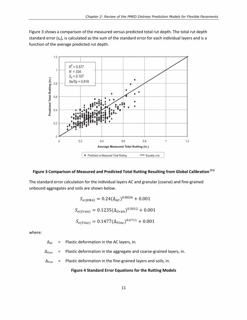
Figure 3 shows a comparison of the measured versus predicted total rut depth. The total rut depth
standard error (se), is calculated as the sum of the standard error for each individual layers and is a
function of the average predicted rut depth.
Figure 3 Comparison of Measured and Predicted Total Rutting Resulting from Global Calibration (11)
The standard error calculation for the individual layers AC and granular (coarse) and fine-grained
unbound aggregates and soils are shown below.
𝑆𝑒(𝐻𝑀𝐴) = 0.24(Δ𝐴𝐶)0.8026 + 0.001
𝑆𝑒(𝐺𝑟𝑎𝑛) = 0.1235(Δ𝐺𝑟𝑎𝑛)0.5012 + 0.001
𝑆𝑒(𝐹𝑖𝑛𝑒) = 0.1477(Δ𝐹𝑖𝑛𝑒)0.6711 + 0.001
where:
∆AC = Plastic deformation in the AC layers, in.
∆Gran = Plastic deformation in the aggregate and coarse-grained layers, in.
∆Fine = Plastic deformation in the fine-grained layers and soils, in.
Figure 4 Standard Error Equations for the Rutting Models

Calibration of the AASHTOWare Pavement ME Design Performance Models for Flexible Pavements in Idaho
12
Load Associated Cracking Prediction Models
The PMED calculates two types of load-related fatigue cracking, bottom-up (alligator) cracking and
top-down (longitudinal) cracking. Once E* and critical tensile strains at the critical locations are
computed (for a given analysis period, traffic load, and environmental location), the allowable number
of repetitions to (alligator or longitudinal) fatigue cracking failure (Nf) is calculated using the following
equations:
𝑵𝒇−𝑨𝑪 = 𝒌𝒇𝟏(𝑪)(𝑪𝑯)𝜷𝒇𝟏(𝜺𝒕)𝒌𝒇𝟐𝜷𝒇𝟐(𝑬𝑨𝑪)𝒌𝒇𝟑𝜷𝒇𝟑
𝐶 = 10𝑀
𝑀 = 4.84 (𝑉𝑏𝑒
𝑉𝑎 + 𝑉𝑏𝑒− 0.69)
where:
Nf-AC = Allowable number of axle-load applications for a flexible pavement and AC overlays
εt = Tensile strain at critical locations and calculated by the structural response model, in./in.
EAC = Dynamic modulus of the AC measured in compression, psi
kf1, kf2, kf3 = Global field calibration coefficients (kf1 = 0.007566, kf2 = +3.9492, and, kf3 = +1.281)
βf1 , βf2 , βf3 = Local or mixture specific field calibration constants; for the global calibration effort, these constants were set to 1.0.
Vbe = Effective asphalt content by volume, percent
Va = Percent air voids in the AC mixture
CH = Thickness correction term, dependent on type of cracking
For bottom-up or alligator cracking:
𝐶𝐻 =1
0.000398 +0.003602
1 + 𝑒(11.02−3.49𝐻𝐴𝐶)
For top-down or longitudinal cracking:
𝐶𝐻 =1
0.01 +12.00
1 + 𝑒(15.676−2.8186𝐻𝐴𝐶)
Figure 5 PMED Equations for the Allowable Number of Traffic Repetitions to Fatigue Damage

Chapter 2: Review of the PMED Distress Prediction Models for Flexible Pavements
13
The accumulative alligator and longitudinal fatigue damage (∑D) is calculated as the linear sum
(Miner’s hypothesis) of the ratio of the predicted to the allowable number of traffic repetitions in a
specific environmental condition as shown below. This is done within a specific time increment and
axle load interval for each axle type in the analysis.
𝑫𝑰 = ∑(∆𝑫𝑰)𝒋,𝒎,𝒍,𝒑,𝑻 = ∑ (𝒏
𝑵𝒇−𝑨𝑪)
𝒋,𝒎,𝒍,𝒑,𝑻
where:
n = Actual number of axle-load applications within a specific time period
j = Axle-load interval
m = Axle-load type (single, tandem, tridem, or quad)
l = Truck type using the truck classification groups included in PMED
p = Month
T = Median temperature for the five temperature intervals or quintiles used to subdivide each month, °F
Figure 6 PMED Equation for the Damage Ratio
The alligator cracking model does not consider an endurance limit. The fatigue damage is transformed
into bottom-up alligator fatigue cracking by using the equation given below.
𝑭𝑪𝑩𝒐𝒕𝒕𝒐𝒎 = (𝟏
𝟔𝟎) (
𝑪𝟒
𝟏 + 𝒆(𝑪𝟏𝑪𝟏∗ +𝑪𝟐𝑪𝟐
∗ 𝑳𝒐𝒈(𝑫𝑰𝑩𝒐𝒕𝒕𝒐𝒎∗𝟏𝟎𝟎)))
where:
FCBottom = Area of alligator cracking that initiates at the bottom of the AC layers, percent of total lane area
DIBottom = Cumulative damage index at the bottom of the AC layers
C1,2,4 = Transfer function regression constants; C 4 = 6,000; C 1 =1.00; and C 2 =1.00
𝐶1∗ = −2𝐶2
∗
𝐶2∗ = −2.40874 − 39.748(1 + 𝐻𝐴𝐶)−2.856
Figure 7 Bottom-Up Cracking Transfer Function

Calibration of the AASHTOWare Pavement ME Design Performance Models for Flexible Pavements in Idaho
14
Figure 8 illustrates the comparison of the cumulative fatigue damage and measured alligator cracking.
Figure 8 Comparison of Cumulative Fatigue Damage and Measured Alligator Cracking Resulting from
Global Calibration Process (11)
Figure 9 below shows a comparison between the measured and predicted lengths of longitudinal
cracking (top-down cracking).
Figure 9 Comparison of Cumulative Fatigue Damage and Measured Alligator Cracking Resulting from
Global Calibration Process (11)

Chapter 2: Review of the PMED Distress Prediction Models for Flexible Pavements
15
Fatigue damage associated with longitudinal cracking is determined from the following equation:
𝑭𝑪𝑻𝒐𝒑 = 𝟏𝟎. 𝟓𝟔 (𝑪𝟒
𝟏 + 𝒆(𝑪𝟏−𝑪𝟐𝑳𝒐𝒈(𝑫𝑰𝑻𝒐𝒑)))
where:
FCTop = Length of longitudinal cracks that initiate at the top of the AC layer, ft/mi
DITop = Cumulative damage index near the top of the AC surface
C1, 2,4 = Transfer function regression constants; C 1 = 7.00; C 2 = 3.5; and C 4 = 1,000
Figure 10 Top-Down Transfer Function
The standard error, for the alligator cracking prediction equation is a function of the average predicted
area of alligator cracks.
𝑺𝒆(𝑨𝒍𝒍𝒊𝒈𝒂𝒕𝒐𝒓) = 𝟏. 𝟏𝟑 +𝟏𝟑
𝟏 + 𝒆𝟕.𝟓𝟕−𝟏𝟓𝑳𝒐𝒈(𝑭𝑪𝑩𝒐𝒕𝒕𝒐𝒎+𝟎.𝟎𝟎𝟎𝟏)
The standard error, for the longitudinal cracking prediction equation is a function of the average
predicted length of the longitudinal cracks.
𝑺𝒆(𝑳𝒐𝒏𝒈) = 𝟐𝟎𝟎 +𝟐𝟑𝟎𝟎
𝟏 + 𝒆𝟏.𝟎𝟕𝟐−𝟐.𝟏𝟔𝟓𝟒𝑳𝒐𝒈(𝑭𝑪𝑻𝒐𝒑+𝟎.𝟎𝟎𝟎𝟏)
Figure 11 Standard Error Equations for Bottom-Up and Top-Down Cracking
For the cement treated base (CTB) layers, PMED uses the models shown below to predict the
fatigue behavior of these layers.

Calibration of the AASHTOWare Pavement ME Design Performance Models for Flexible Pavements in Idaho
16
𝑵𝒇−𝑪𝑻𝑩 = 𝟏𝟎[𝒌𝒄𝟏𝜷𝒄𝟏(
𝝈𝒕𝑴𝑹
)
𝒌𝒄𝟐𝜷𝒄𝟐]
𝑭𝑪𝑪𝑻𝑩 = 𝑪𝟏 +𝑪𝟐
𝟏 + 𝒆(𝑪𝟑−𝑪𝟒𝑳𝒐𝒈(𝑫𝑰𝑪𝑻𝑩))
where:
Nf-CTB = Allowable number of axle-load applications for a semi-rigid pavement
σt = Tensile stress at the bottom of the CTB layer, psi
MR = 28-day modulus of rupture for the CTB layer, psi
DICTB = Cumulative damage index of the CTB or cementitious layer and determined in accordance with Eq. 14
kc1,c2 = Global calibration coefficients—Undefined because prediction equation was never calibrated; these values are set to 1.0 in the software. From other studies, kc1 =0.972 and kc2 = 0.0825
βc1,c2 = Local calibration constants; these values are set to 1.0 in the software
FCCTB = Area of fatigue cracking, ft2
C1,2,3,4 = Transfer function regression constants; C 1 =1.0, C 2 =1.0, C 3 =0, and C 4 =1,000. To date, this transfer function has not been calibrated and these values will change when it is calibrated
Figure 12 Fatigue Cracking Prediction Model for CTB Layers
The computational analysis of incremental fatigue cracking for a semi-rigid pavement uses the damaged
modulus approach. In summary, the elastic modulus of the CTB layer decreases as the damage index,
DICTB, increases. The equation below is used to calculate the damaged elastic modulus within each
season or time period for the CTB and other pavement layers. One may notice that the equation below
has not been globally calibrated due to the difficulty associated with obtaining field section design input
and performance data.

Chapter 2: Review of the PMED Distress Prediction Models for Flexible Pavements
17
𝑬𝑪𝑻𝑩𝑫(𝒕)
= 𝑬𝑪𝑻𝑩𝑴𝒊𝒏 + (
𝑬𝑪𝑻𝑩𝑴𝒂𝒙 − 𝑬𝑪𝑻𝑩
𝑴𝒊𝒏
𝟏 + 𝒆(−𝟒+𝟏𝟒(𝑫𝑰𝑪𝑻𝑩)))
where:
𝐸𝐶𝑇𝐵𝐷(𝑡)
= Equivalent damaged elastic modulus at time t for the CTB layer, psi
𝐸𝐶𝑇𝐵𝑀𝑖𝑛 = Equivalent elastic modulus for the total destruction of the CTB layer, psi
𝐸𝐶𝑇𝐵𝑀𝑎𝑥 = 28-day elastic modulus of the intact CTB layer, no damage, psi
Figure 13 CTB Layer Damaged Modulus Equation
Non-Load Associated Transverse Cracking Prediction Model
The extent of transverse cracking expected in a pavement system is predicted by relating the crack
depth to the amount of cracking (crack frequency) by the equation shown below.
𝑻𝑪 = 𝜷𝒕𝟏𝑵 [𝟏
𝝈𝒅𝑳𝒐𝒈 (
𝑪𝒅
𝑯𝑨𝑪)]
where: TC = Observed amount of thermal cracking, ft/mi βt1 = Regression coefficient determined through global calibration (400) N[z] = Standard normal distribution evaluated at [z] σd = Standard deviation of the log of the depth of cracks in the pavement (0.769), in. Cd = Crack depth, in. HAC = Thickness of AC layers, in.
Figure 14 PMED Thermal Cracking Model
The MEPDG manual of practice includes a comparison between the measured and predicted cracking for
each hierarchical input level.(4,10,11) The standard error for the transverse cracking prediction equations
include:
𝑆𝑒(𝐿𝑒𝑣𝑒𝑙 1) = −0.1468(𝑇𝐶 + 65.027)
𝑆𝑒(𝐿𝑒𝑣𝑒𝑙 2) = −0.2841(𝑇𝐶 + 55.462)
𝑆𝑒(𝐿𝑒𝑣𝑒𝑙 3) = −0.3972(𝑇𝐶 + 20.422)
Figure 15 Standard Error Equations for the Thermal Cracking

Calibration of the AASHTOWare Pavement ME Design Performance Models for Flexible Pavements in Idaho
18
For a given thermal cooling cycle, Paris law is used to estimate the crack propagation as shown
below.
∆𝑪 = 𝑨(∆𝑲)𝒏
𝐴 = 𝑘𝑡𝛽𝑡10[4.389−2.52𝐿𝑜𝑔(𝐸𝐴𝐶𝜎𝑚𝑛)]
𝜂 = 0.8 (1 +1
𝑚)
where:
ΔC = Change in the crack depth due to a cooling cycle
ΔK = Change in the stress intensity factor due to a cooling cycle
A, n = Fracture parameters for the AC mixture
kt = Coefficient determined through global calibration for each input level (Level 1 = 1.5; Level 2 = 0.5; and Level 3 = 1.5)
EAC = AC indirect tensile modulus, psi
σm = Mixture tensile strength, psi
m = Derived from the indirect tensile creep compliance curve measured in the laboratory
βt = Local or mixture calibration coefficient
𝐾 = 𝜎𝑡𝑖𝑝⌊0.45 + 1.99(𝐶0)0.56⌋
σtip = Far-field stress from pavement response model at depth of crack tip, psi
Co = Current crack length, ft
Figure 16 Paris Law for Crack Propagation
Reflection Cracking in AC Overlays
For the AC over existing flexible and AC over rigid pavements overlay options PMED uses a simple
empirical model, based on field observations, for the prediction of reflective cracking. This model
predicts the percentage of cracks that propagate through the overlay as a function of time and AC
overlay thickness using the equations shown below.
Chapter 2: Review of the PMED Distress Prediction Models for Flexible Pavements
19
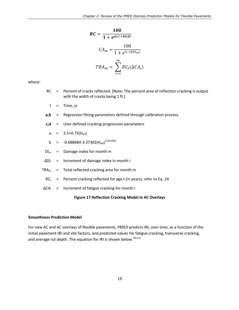
𝑹𝑪 = 𝟏𝟎𝟎
𝟏 + 𝒆𝒂(𝒄)+𝒃𝒕(𝒅)
𝐶𝐴𝑚 =100
1 + 𝑒6−(6𝐷𝐼𝑚)
𝑇𝑅𝐴𝑚 = ∑ 𝑅𝐶𝑡(Δ𝐶𝐴𝑖)
𝑚
𝑖=1
where:
RC = Percent of cracks reflected. [Note: The percent area of reflection cracking is output with the width of cracks being 1 ft.]
t = Time, yr
a,b = Regression fitting parameters defined through calibration process
c,d = User-defined cracking progression parameters
a = 3.5+0.75(Heff)
b = -0.688684-3.37302(Heff)-0.915469
DIm = Damage index for month m
ΔDIi = Increment of damage index in month i
TRAm = Total reflected cracking area for month m
RCt = Percent cracking reflected for age t (in years), refer to Eq. 24
ΔCAi = Increment of fatigue cracking for month i
Figure 17 Reflection Cracking Model in AC Overlays
Smoothness Prediction Model
For new AC and AC overlays of flexible pavements, PMED predicts IRI, over time, as a function of the
initial pavement IRI and site factors, and predicted values for fatigue cracking, transverse cracking,
and average rut depth. The equation for IRI is shown below.(10,11)

Calibration of the AASHTOWare Pavement ME Design Performance Models for Flexible Pavements in Idaho
20
𝑰𝑹𝑰 = 𝑰𝑹𝑰𝒐 + 𝑪𝟏(𝑹𝑫) + 𝑪𝟐(𝑭𝑪𝑻𝒐𝒕𝒂𝒍) + 𝑪𝟑(𝑻𝑪) + 𝑪𝟒(𝑺𝑭)
𝑆𝐹 = 𝐴𝑔𝑒1.5{𝑙𝑛[(𝑝𝑟𝑒𝑐𝑖𝑝 + 1)(𝐹𝐼 + 1)𝑝02]} + {𝑙𝑛[(𝑝𝑟𝑒𝑐𝑖𝑝 + 1)(𝑃𝐼 + 1)𝑝200]}
where:
IRI0 = Initial IRI after construction, in/mi
SF = Site factor.
FCTotal = Area of fatigue cracking (combined wheel path alligator, longitudinal, and reflection cracking), percent of total lane area (transverse width of crack is assumed to be 1-ft wide)
TC = Length of transverse cracking (including transverse reflection cracks in existing AC pavements), ft/mi
RD = Average rut depth, in.
C1,2,3,4 = Calibration coefficients; C1 = 40.0, C2 = 0.400, C3 = 0.008, C4 = 0.015.
Age = Pavement age, yr
PI = Percent plasticity index of the soil
FI = Average annual freezing index, °F days
Precip = Average annual precipitation or rainfall, in.
p02 = Percent passing the 0.02 mm sieve
p200 = Percent passing the 0.075 mm sieve
Figure 18 Smoothness Prediction Model
PMED Calibration and Implementation Efforts by State DOTs
A number of state DOTs have implemented or plan to implement the PMED. There are also several
DOT’s who have no PMED implementation plans at this time. In a recent agency summary, conducted by
the AASHTO Pavement ME National User Group, 13 DOTs have implemented the PMED, 35 DOTs,
including Idaho, are planning to implement within the next five years, and 5 DOTs disclosed no plans for
implementation (Figure 19).(12)

Chapter 2: Review of the PMED Distress Prediction Models for Flexible Pavements
21
Figure 19 Summary of Agency PMED Implementation(12)
Arizona
The Arizona DOT is one of the lead states for PMED implementation. Working with the Arizona State
University, Arizona DOT initiated a long-term research project beginning in 1999. The main project
objective was to develop performance-related specifications for asphalt pavements in Arizona based on
the PMED.(13) This research project focused on development of Arizona-specific PMED inputs for asphalt
binders and mixtures, unbound base materials and subgrade soils, climate, and traffic characteristics.
In addition, a research effort was conducted to develop local calibration coefficients for asphalt rutting,
load-related alligator and longitudinal cracking, and IRI of new flexible pavements. A total of 22, 25, and
37 pavement sections, respectively, with performance and material characterization data were obtained
from LTPP and Arizona DOT databases.(14) A trial and error method was used to determine local
calibration coefficients that resulted in the least squared error and zero sum of standard error between
PMED predicted and field-measured values. The recommended calibration coefficients for Arizona are
summarized in Table 1.

Calibration of the AASHTOWare Pavement ME Design Performance Models for Flexible Pavements in Idaho
22
Table 1 Arizona Local Calibration Coefficients(14)
Distress Model Distress Type/Layer Calibration Coefficient
Rutting
AC, (βr1, βr2, βr3) 3.63, 1.10, 0.70
Granular Base, (βB1) 0.111
Subgrade, (βs1) 1.38
Fatigue Cracking
Fatigue Model, (βf1, βf2 and βf3) 0.729, 0.800,0.800
Bottom-Up Transfer Function (C1, C2) 0.732, 0.732
Top-Down Transfer Function (C1, C2) 1.607, 0.803
IRI Smoothness (C1, C2, C3, C4) 5.455,0.354,0.008,0.015
California
In 2005, California Department of Transportation (Caltrans) approved the adoption of PMED for
concrete pavements only using globally-calibrated coefficients.(15) Asphalt pavements are characterized
using CalME, a Caltrans-developed ME design procedure.
Montana
For Montana, the PMED implementation effort was divided into three phases. Phase I included
identifying test sections and preliminary data (e.g., pavement structure, materials, performance) needed
for calibration.(11) Phase II involved data collection and analysis of the PMED performance prediction
models for climate, materials, and design strategies in Montana. Phase III included additional data
collection efforts for updating the calibration coefficients.(16,17,18) In the Montana DOT study, results from
NCHRP 1-40B, User Manual and Local Calibration Guide for the Mechanistic-Empirical Pavement Design
Guide and Software, were used to determine bias and standard error and compared to the standard
error from the original calibration process completed under NCHRP Project 1-37A. Bias was found for
most of the distress transfer functions. Global calibration coefficients included in PMED v0.9 were
initially used to predict the distresses and IRI of the Montana test sections and to determine model bias.
These runs were considered a part of the validation process, similar to the process used under NCHRP
Project 1-40B and NCHRP Project 9-30, Experimental Plan for Calibration and Validation of HMA
Performance Models for Mix and Structural Design. Table 2 includes the local calibration coefficients for
Montana.
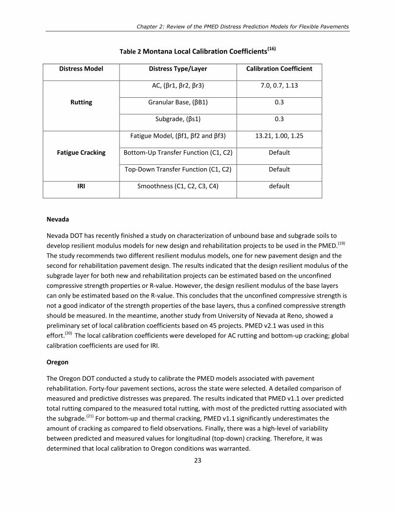
Chapter 2: Review of the PMED Distress Prediction Models for Flexible Pavements
23
Table 2 Montana Local Calibration Coefficients(16)
Distress Model Distress Type/Layer Calibration Coefficient
Rutting
AC, (βr1, βr2, βr3) 7.0, 0.7, 1.13
Granular Base, (βB1) 0.3
Subgrade, (βs1) 0.3
Fatigue Cracking
Fatigue Model, (βf1, βf2 and βf3) 13.21, 1.00, 1.25
Bottom-Up Transfer Function (C1, C2) Default
Top-Down Transfer Function (C1, C2) Default
IRI Smoothness (C1, C2, C3, C4) default
Nevada
Nevada DOT has recently finished a study on characterization of unbound base and subgrade soils to
develop resilient modulus models for new design and rehabilitation projects to be used in the PMED.(19)
The study recommends two different resilient modulus models, one for new pavement design and the
second for rehabilitation pavement design. The results indicated that the design resilient modulus of the
subgrade layer for both new and rehabilitation projects can be estimated based on the unconfined
compressive strength properties or R-value. However, the design resilient modulus of the base layers
can only be estimated based on the R-value. This concludes that the unconfined compressive strength is
not a good indicator of the strength properties of the base layers, thus a confined compressive strength
should be measured. In the meantime, another study from University of Nevada at Reno, showed a
preliminary set of local calibration coefficients based on 45 projects. PMED v2.1 was used in this
effort.(20) The local calibration coefficients were developed for AC rutting and bottom-up cracking; global
calibration coefficients are used for IRI.
Oregon
The Oregon DOT conducted a study to calibrate the PMED models associated with pavement
rehabilitation. Forty-four pavement sections, across the state were selected. A detailed comparison of
measured and predictive distresses was prepared. The results indicated that PMED v1.1 over predicted
total rutting compared to the measured total rutting, with most of the predicted rutting associated with
the subgrade.(21) For bottom-up and thermal cracking, PMED v1.1 significantly underestimates the
amount of cracking as compared to field observations. Finally, there was a high-level of variability
between predicted and measured values for longitudinal (top-down) cracking. Therefore, it was
determined that local calibration to Oregon conditions was warranted.
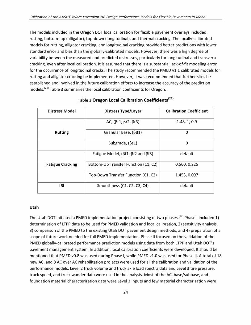
Calibration of the AASHTOWare Pavement ME Design Performance Models for Flexible Pavements in Idaho
24
The models included in the Oregon DOT local calibration for flexible pavement overlays included:
rutting, bottom- up (alligator), top-down (longitudinal), and thermal cracking. The locally-calibrated
models for rutting, alligator cracking, and longitudinal cracking provided better predictions with lower
standard error and bias than the globally-calibrated models. However, there was a high degree of
variability between the measured and predicted distresses, particularly for longitudinal and transverse
cracking, even after local calibration. It is assumed that there is a substantial lack-of-fit modeling error
for the occurrence of longitudinal cracks. The study recommended the PMED v1.1 calibrated models for
rutting and alligator cracking be implemented. However, it was recommended that further sites be
established and involved in the future calibration efforts to increase the accuracy of the prediction
models.(21) Table 3 summaries the local calibration coefficients for Oregon.
Table 3 Oregon Local Calibration Coefficients(21)
Distress Model Distress Type/Layer Calibration Coefficient
Rutting
AC, (βr1, βr2, βr3) 1.48, 1, 0.9
Granular Base, (βB1) 0
Subgrade, (βs1) 0
Fatigue Cracking
Fatigue Model, (βf1, βf2 and βf3) default
Bottom-Up Transfer Function (C1, C2) 0.560, 0.225
Top-Down Transfer Function (C1, C2) 1.453, 0.097
IRI Smoothness (C1, C2, C3, C4) default
Utah
The Utah DOT initiated a PMED implementation project consisting of two phases.(22) Phase I included 1)
determination of LTPP data to be used for PMED validation and local calibration, 2) sensitivity analysis,
3) comparison of the PMED to the existing Utah DOT pavement design methods, and 4) preparation of a
scope of future work needed for full PMED implementation. Phase II focused on the validation of the
PMED globally-calibrated performance prediction models using data from both LTPP and Utah DOT’s
pavement management system. In addition, local calibration coefficients were developed. It should be
mentioned that PMED v0.8 was used during Phase I, while PMED v1.0 was used for Phase II. A total of 18
new AC, and 8 AC over AC rehabilitation projects were used for all the calibration and validation of the
performance models. Level 2 truck volume and truck axle load spectra data and Level 3 tire pressure,
truck speed, and truck wander data were used in the analysis. Most of the AC, base/subbase, and
foundation material characterization data were Level 3 inputs and few material characterization were

Chapter 2: Review of the PMED Distress Prediction Models for Flexible Pavements
25
available at Level 2. The Natural Resources Conservation Service was used for subgrade soil
characterization. Data included in the PMED for Utah and surrounding states was used to create virtual
site-specific climatic information. The Utah DOT calibration study showed, for new flexible pavements
and AC over AC rehabilitation design, the globally-calibrated alligator cracking model predictions were
relatively good for low to moderate cracking. There were no pavement sections in Utah with significant
alligator cracking to verify sever cracking model predictions. The globally-calibrated transverse cracking
model predictions were adequate for newly constructed pavements with Superpave binders. Good
agreement was found between measured and predicted IRI using the PMED globally-calibrated IRI
prediction model. Only the rutting prediction models needed to be calibrated to reflect Utah
conditions.(22) Table 4 presents the Utah’s local calibration coefficients.
Table 4 Utah Local Calibration Coefficients(22)
Distress Model Distress Type/Layer Calibration Coefficient
Rutting
AC, (βr1, βr2, βr3) 0.560, 1.00, 1.00
Granular Base, (βB1) 0.604
Subgrade, (βs1) 0.4
Fatigue Cracking
Fatigue Model, (βf1, βf2 and βf3) default
Bottom-Up Transfer Function (C1, C2) default
Top-Down Transfer Function (C1, C2) default
IRI Smoothness (C1, C2, C3, C4) default
Washington
The flexible pavement distress models, excluding the IRI model, were successfully calibrated to
Washington State conditions using MEPDG version 1.0.(23) The final local calibration coefficients for
Washington State are shown in Table 5. Based on the outcome of the calibration process, the developed
coefficients were found to be reasonable, and applicable to more than 90 percent of WSDOT flexible
pavements Recommendations for PMED implementation and improvement include:
1. Local agencies need to balance the accuracy of inputs and costs.
2. Local calibration, along with implementation, is a continual process. Users need to allow sensible
bias between local observations and model prediction. The final design should be within a
reasonable range.
3. Agencies with similar materials and climates may combine data to increase the number of
pavement sections for local calibration.

Calibration of the AASHTOWare Pavement ME Design Performance Models for Flexible Pavements in Idaho
26
4. Ongoing and future work that inspects and evaluates the PMED performance prediction models
and software function should continue to be monitored.(23)
Table 5 Washington State Local Calibration Coefficients (23)
Distress Model Distress Type/Layer Calibration Coefficient
Rutting
AC, (βr1, βr2, βr3) 1.05, 1.109, 1.1
Granular Base, (βB1) Default
Subgrade, (βs1) 0
Fatigue Cracking
Fatigue Model, (βf1, βf2 and βf3) 0.96, 0.97, 1.03
Bottom-Up Transfer Function (C1, C2) 1.071, 1.0
Top-Down Transfer Function (C1, C2) 6.42, 3.596
IRI Smoothness (C1, C2, C3, C4) Could not locally calibrate
due to software bug
Wyoming
Wyoming DOT has been actively working toward the implementation of the Mechanistic-Empirical
design. Their plan consists of two phases: Phase 1 includes development of the database, and Phase 2
focuses on data analyses, recommendations, trial designs and examples, design comparisons, design
guidelines, and implementation.(24,25) The traffic and climate inputs have been characterized and the
DOT is focusing on a comprehensive field and laboratory test program for subgrade soils. To efficiently
store the results from the field and laboratory testing results, an electronic database (WYOMEP) was
developed in Microsoft Access 2013. Specific data or inputs requested by user are efficiently and easily
sorted, filtered, and queried in the database. Wyoming DOT will continue to populate the database with
future construction projects. A set of preliminary local calibration coefficients, primarily for primary and
secondary roadways were developed in 2012.(6,24) The local calibration coefficients for Wyoming and are
shown in Table 6.

Chapter 2: Review of the PMED Distress Prediction Models for Flexible Pavements
27
Table 6 Wyoming Local Calibration Coefficients(6)
Distress Model Distress Type/Layer Calibration Coefficient
Rutting
AC, (βr1, βr2, βr3) 1.0896, 1.0, 1.0
Granular Base, (βB1) 0.9475
Subgrade, (βs1) 0.6897
Fatigue Cracking
Fatigue Model, (βf1, βf2 and βf3) 1.00, 1.00, 1.00
Bottom-Up Transfer Function (C1, C2) 0.4951,1.469
Top-Down Transfer Function (C1, C2) Default
Thermal Cracking Thermal Fracture (K1,K2) 7.5,7.5
IRI Smoothness (C1, C2, C3, C4) 20.53,0.4094,0.00179,0.015
State DOT PMED Implementation Summary
Based on review of DOT PMED calibration and implementation activities, successful PMED
implementation is accomplished with comprehensive material and traffic characterization. Development
of accompanying database (library) will greatly enhance future calibration efforts. Distress prediction
models may require local calibration to improve predication accuracy and reduce bias. Understanding
the sensitivity of each input and establishing reasonable ranges for key design inputs are extremely
important.
In a study conducted by the Federal Highway Administration (FHWA), agency recommendations for local
calibration include evaluating measured distress data and ensuring it is consistent with the distress
definitions in the PMED.(26) In addition, material, traffic, and climate parameters should be reviewed to
determine if changes to default inputs are necessary to model pavement sections accurately. Some of
the other challenges identified were the lack of distress or pavement material information, limited
ranges of distress values and pavement service life, and fewer sites than needed to conduct statistically
meaningful calibration.
Pavement performance data measured accurately over time in a manner consistent with PMED
requirements is essential for implementation and local calibration.(4,5,10) Many DOTs (including ITD)
collect cracking data in a format inconsistent with the PMED recommended method. Therefore, to
conduct the local calibration, cracking data may require additional analysis to format to the PMED
method. Additional agencies calibration coefficients were obtained from the literature and included in
the summary tables that follow.(27,28,29,30,31) A summary of the local calibration coefficients for rutting,

Calibration of the AASHTOWare Pavement ME Design Performance Models for Flexible Pavements in Idaho
28
fatigue cracking (alligator and longitudinal), thermal cracking, and IRI are shown in Table 7 through Table
10, respectively.
Table 7 Summary of Local Calibration Coefficients for Rutting
State AC Granular Base Subgrade
βr1 βr2 βr3 βB1 βs1
Arizona 3.63 1.10 0.70 0.111 1.38
Montana 7 0.7 1.13 0.30 0.30
Oregon 1.48 1.00 0.9 0 0
Utah 0.56 1.00 1.00 0.604 0.40
Washington 1.05 1.109 1.10 1.00 0.00
Wyoming 1.0896 1.00 1.00 0.9475 0.6897
Arkansas 1.20 1.00 0.80 1.00 0.50
Kansas
Conventional 1.50 0.90 1.00 0.50 0.50
PMA * 2.50 1.15 1.00 0.50 0.50
Superpave 1.50 1.20 1.00 0.50 0.50
North Carolina 0.983 1.00 1.00 1.58 1.10
PMA* = Polymer Modified Asphalt
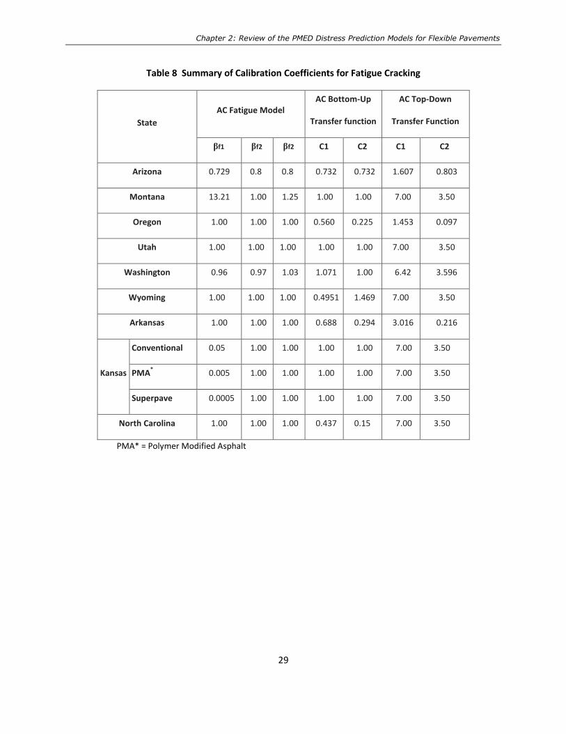
Chapter 2: Review of the PMED Distress Prediction Models for Flexible Pavements
29
Table 8 Summary of Calibration Coefficients for Fatigue Cracking
State AC Fatigue Model
AC Bottom-Up
Transfer function
AC Top-Down
Transfer Function
βf1 βf2 βf2 C1 C2 C1 C2
Arizona 0.729 0.8 0.8 0.732 0.732 1.607 0.803
Montana 13.21 1.00 1.25 1.00 1.00 7.00 3.50
Oregon 1.00 1.00 1.00 0.560 0.225 1.453 0.097
Utah 1.00 1.00 1.00 1.00 1.00 7.00 3.50
Washington 0.96 0.97 1.03 1.071 1.00 6.42 3.596
Wyoming 1.00 1.00 1.00 0.4951 1.469 7.00 3.50
Arkansas 1.00 1.00 1.00 0.688 0.294 3.016 0.216
Kansas
Conventional 0.05 1.00 1.00 1.00 1.00 7.00 3.50
PMA* 0.005 1.00 1.00 1.00 1.00 7.00 3.50
Superpave 0.0005 1.00 1.00 1.00 1.00 7.00 3.50
North Carolina 1.00 1.00 1.00 0.437 0.15 7.00 3.50
PMA* = Polymer Modified Asphalt

Calibration of the AASHTOWare Pavement ME Design Performance Models for Flexible Pavements in Idaho
30
Table 9 Summary of Local Calibration Coefficients for Transverse Cracking
State Calibration Coefficient
(βt1)
Arizona -
Montana 0.25
Oregon -
Utah -
Washington -
Wyoming 7.5
Arkansas -
Kansas
Conventional 2.00
PMA* 2.00
Superpave 3.50
North Carolina -
PMA* = Polymer Modified Asphalt

Chapter 2: Review of the PMED Distress Prediction Models for Flexible Pavements
31
Table 10 Summary of Local Calibration Coefficients for IRI
Calibration Coefficients C1 C2 C3 C4
Arizona 5.455 0.354 0.008 0.015
Montana 40 0.4 0.008 0.015
Oregon 40 0.4 0.008 0.015
Utah 40 0.4 0.008 0.015
Washington 40 0.4 0.008 0.015
Wyoming 20.53 0.4094 0.00179 0.015
Arkansas 40 0.4 0.008 0.015
Kansas
Conventional 40 0.4 0.008 0.015
PMA* 40 0.4 0.008 0.015
Superpave 40 0.4 0.008 0.015
North Carolina 40 0.4 0.008 0.015
PMA* = Polymer Modified Asphalt

Calibration of the AASHTOWare Pavement ME Design Performance Models for Flexible Pavements in Idaho
32
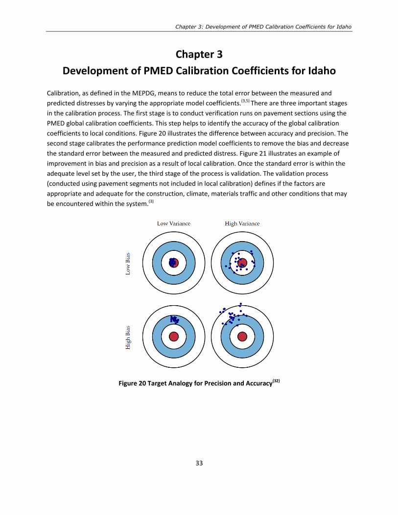
Chapter 3: Development of PMED Calibration Coefficients for Idaho
33
Chapter 3
Development of PMED Calibration Coefficients for Idaho
Calibration, as defined in the MEPDG, means to reduce the total error between the measured and
predicted distresses by varying the appropriate model coefficients.(3,5) There are three important stages
in the calibration process. The first stage is to conduct verification runs on pavement sections using the
PMED global calibration coefficients. This step helps to identify the accuracy of the global calibration
coefficients to local conditions. Figure 20 illustrates the difference between accuracy and precision. The
second stage calibrates the performance prediction model coefficients to remove the bias and decrease
the standard error between the measured and predicted distress. Figure 21 illustrates an example of
improvement in bias and precision as a result of local calibration. Once the standard error is within the
adequate level set by the user, the third stage of the process is validation. The validation process
(conducted using pavement segments not included in local calibration) defines if the factors are
appropriate and adequate for the construction, climate, materials traffic and other conditions that may
be encountered within the system.(3)
Figure 20 Target Analogy for Precision and Accuracy(32)
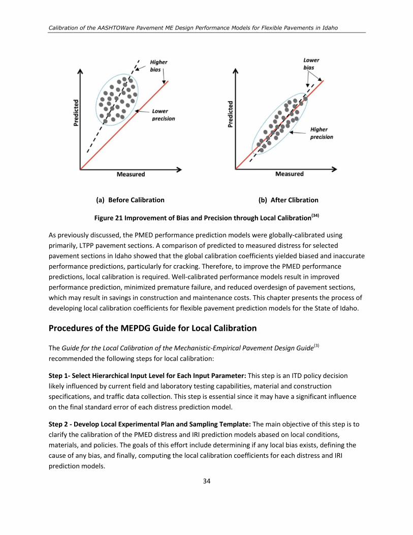
Calibration of the AASHTOWare Pavement ME Design Performance Models for Flexible Pavements in Idaho
34
(a) Before Calibration (b) After Clibration
Figure 21 Improvement of Bias and Precision through Local Calibration(34)
As previously discussed, the PMED performance prediction models were globally-calibrated using
primarily, LTPP pavement sections. A comparison of predicted to measured distress for selected
pavement sections in Idaho showed that the global calibration coefficients yielded biased and inaccurate
performance predictions, particularly for cracking. Therefore, to improve the PMED performance
predictions, local calibration is required. Well-calibrated performance models result in improved
performance prediction, minimized premature failure, and reduced overdesign of pavement sections,
which may result in savings in construction and maintenance costs. This chapter presents the process of
developing local calibration coefficients for flexible pavement prediction models for the State of Idaho.
Procedures of the MEPDG Guide for Local Calibration
The Guide for the Local Calibration of the Mechanistic-Empirical Pavement Design Guide(3)
recommended the following steps for local calibration:
Step 1- Select Hierarchical Input Level for Each Input Parameter: This step is an ITD policy decision
likely influenced by current field and laboratory testing capabilities, material and construction
specifications, and traffic data collection. This step is essential since it may have a significant influence
on the final standard error of each distress prediction model.
Step 2 - Develop Local Experimental Plan and Sampling Template: The main objective of this step is to
clarify the calibration of the PMED distress and IRI prediction models abased on local conditions,
materials, and policies. The goals of this effort include determining if any local bias exists, defining the
cause of any bias, and finally, computing the local calibration coefficients for each distress and IRI
prediction models.

Chapter 3: Development of PMED Calibration Coefficients for Idaho
35
Step 3 - Estimate Sample Size for Specific Distress Prediction Models: This step is used to determine the
sample size (number of roadway sections) to check the adequacy of the global calibration coefficients
and determine the local calibration coefficients for each distress model, if needed.
Step 4 - Select Roadway Segments: This step is used to choose the roadway sections and evaluate the
availability and adequacy of existing information and data. During this effort, pavement sections
requiring minimal additional sampling and filed testing are preferred to minimize costs.
Step 5 - Extract and Evaluate Distress and Project Data: After selecting the roadway sections, the next
step is to collect all data and identify any missing data elements that are needed. All data should be
entered into a calibration database.
Step 6 - Conduct Field and Forensic Investigations: This step is divided into three activities. First,
develop a material sampling and testing plan to determine any missing data elements or to validate key
inputs for selected pavement sections. Second, decide whether forensic investigations are required to
confirm the assumptions embedded in the PMED. For instance, the percent of total rutting measured at
the surface that can be assigned to each pavement layer and the location of crack initiation (bottom-up
versus top-down, load-related cracking). Third, re-evaluate the number of roadway sections and data
needed to execute the PMED. The main objective of this activity is to ensure that a sufficient number of
pavement sections are available for the local validation-calibration effort.
Step 7 - Assess Local Bias: In this step, the PMED global calibration coefficients are used to estimate the
performance indicators for each roadway segment (new pavement and rehabilitation strategies). To
validate each distress predication model, the predicated distress values are compared to the measured
ones. Then, determine the standard error and bias of the estimate.
Step 8 - Eliminate Local Bias of Distress and IRI Prediction Models: This step is used to eliminate
significant bias as specified by the agency.
Step 9 - Assess the Standard Error of the Estimate: Determine the difference between the standard
error from the local calibration data set and the standard error derived from the global data set.
Step 10 - Reduce Standard Error of the Estimate: If the user decides that the standard error is too large,
resulting in overly conservative designs at higher reliability levels, revisions to the local calibration
coefficients of the transfer functions or statistical models may be needed This step can be complicated
and may require external revisions to the local calibration parameters or agency-specific values to
improve prediction model precision.
Step 11 - Interpretation of Results, Deciding on Adequacy of Calibration Parameters: The local
standard error of the estimate for each distress and IRI prediction model should be evaluated to
determine the impact on the resulting designs at different reliability levels. A sampling template can be
used to determine the design life of typical site features and pavement structures or rehabilitation

Calibration of the AASHTOWare Pavement ME Design Performance Models for Flexible Pavements in Idaho
36
strategies for different reliability levels. An agency should review the expected pavement/rehabilitation
design life within each cell of the sampling template.
Idaho Local Calibration Procedures
The research team followed the guidelines of the MEPDG to perform the local calibration. The steps
followed are described below:
Hierarchical Input Level Selection for Each Input Parameter
PMED inputs are categorized into four general areas: project inputs, traffic inputs, climatic inputs, and
pavement structure inputs. Project inputs include general information to identify the project, such as
the type of design, construction and traffic opening dates, etc. These inputs also include information
regarding the design criteria (threshold values for distresses and roughness) and reliability level for each
distress selected in the criteria. Traffic, climate, and structure inputs must be completed to
design/analysis a specific pavement structure. A brief listing of input parameters for flexible pavement
design or analysis is presented in Table 11.(3,5) Appendix B includes a summary of all PMED required
inputs for new and rehabilitated flexible pavements.

Chapter 3: Development of PMED Calibration Coefficients for Idaho
37
Table 11 Required Flexible Pavement Input Parameters(3,5)
Input Group Input Parameter
Truck Traffic
Axle Load Distributions (Single, Tandem, Tridem, and Quad)
Truck Volume Distribution
Lane & Directional Truck Distribution
Tire Pressure
Axle Configuration, Tire Spacing
Truck Wander
Traffic Speed
Climate Temperature, Wind Speed, Cloud Cover, Precipitation, Relative Humidity
Material
Properties
Unbound Layers
& Subgrade
Materials
Seasonally Adjusted Resilient Modulus – All Unbound Layers
Classification & Volumetric Properties
Coefficient of Lateral Pressure
Plasticity index, Gradation Parameters, Effective Grain Sizes, Specific
Gravity, Optimum Moisture Contents, Parameters to Define the Soil Water
Characteristic Curve (SWCC)
Bedrock Elastic Modulus

Calibration of the AASHTOWare Pavement ME Design Performance Models for Flexible Pavements in Idaho
38
Table 11 Required Flexible Pavement Input Parameters (Cont.)
Input Group Input Parameter
Material
Properties
Asphalt
Concrete (AC),
Recycled AC
Time-Temperature Dependent AC Dynamic Modulus
AC Creep Compliance & Indirect Tensile Strength
Volumetric Properties
Asphalt Binder Viscosity (Stiffness) Characterization to
Account for Aging
All Materials Except Bedrock
Unit Weight
Poisson’s Ratio
Other Thermal Properties; Conductivity; Heat Capacity;
Surface Absorptivity
Existing Pavement (In Case of
Overlay Design) Condition of Existing Layers
The PMED hierarchical input level feature provides the user flexibility in determining the required input
parameters based on its importance and anticipated funding cost. For flexible pavements, the PMED
includes three input levels for traffic and material properties. Inputs can consist of a mix of hierarchical
levels. Hierarchical input levels include:
Level 1 represents the highest level of accuracy and lowest level of input errors. Input
parameters are measured directly either in the laboratory or in the field. This level of input has
the highest cost in testing and data collection. It is important to note that Level 1 is more
representative of agency or project specific traffic, materials, and climatic inputs.
Level 2 represents an intermediate level of accuracy. Parameters are estimated from
correlations based on limited routine laboratory test results or selected from an agency
database.
Level 3 represents the lowest level of accuracy. Usually, typical default values (best estimates) of
input parameters are used in this level.
The research team studied and evaluated the inputs required to run the latest version of the PMED, and
determined the level of input for each required parameter based on data availability. For the AC, ITD use
six typical Superpave mixes (SP1 to SP6). These typical mixes were characterized and evaluated under
RP193 project, and a database for these mixes’ properties was developed. Thus, properties such as E*
and G* were used from this database based on the mix type and use it in the software as level one.
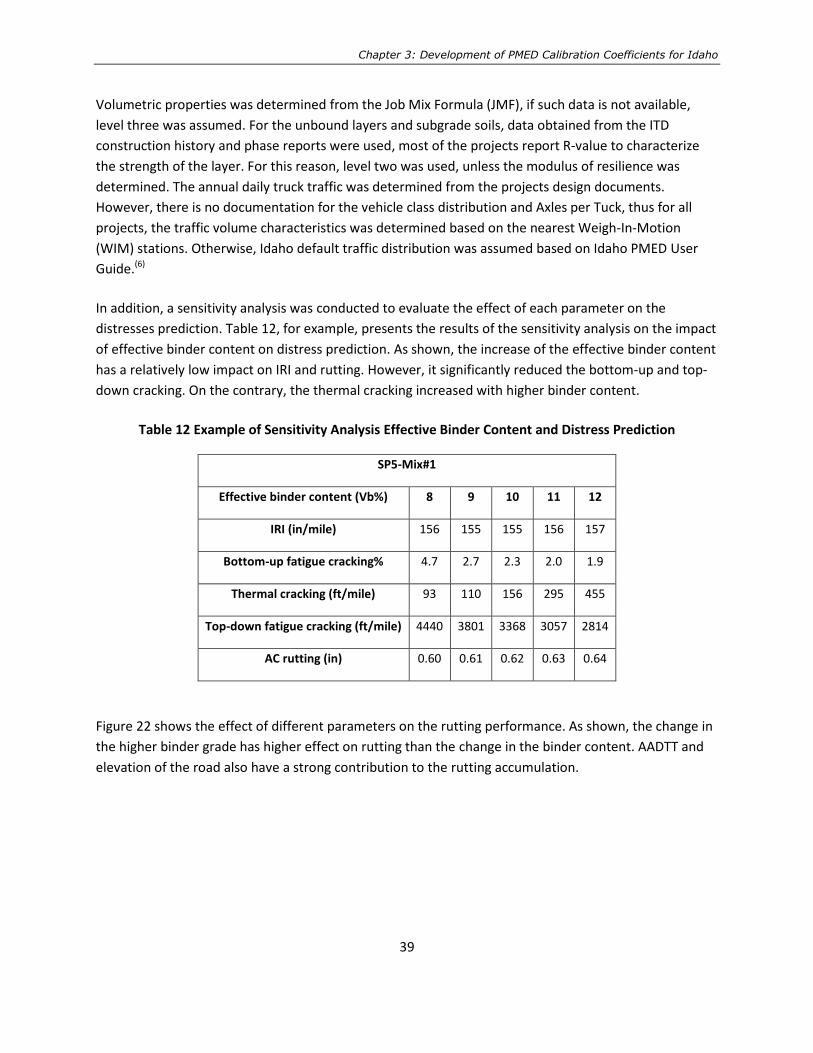
Chapter 3: Development of PMED Calibration Coefficients for Idaho
39
Volumetric properties was determined from the Job Mix Formula (JMF), if such data is not available,
level three was assumed. For the unbound layers and subgrade soils, data obtained from the ITD
construction history and phase reports were used, most of the projects report R-value to characterize
the strength of the layer. For this reason, level two was used, unless the modulus of resilience was
determined. The annual daily truck traffic was determined from the projects design documents.
However, there is no documentation for the vehicle class distribution and Axles per Tuck, thus for all
projects, the traffic volume characteristics was determined based on the nearest Weigh-In-Motion
(WIM) stations. Otherwise, Idaho default traffic distribution was assumed based on Idaho PMED User
Guide.(6)
In addition, a sensitivity analysis was conducted to evaluate the effect of each parameter on the
distresses prediction. Table 12, for example, presents the results of the sensitivity analysis on the impact
of effective binder content on distress prediction. As shown, the increase of the effective binder content
has a relatively low impact on IRI and rutting. However, it significantly reduced the bottom-up and top-
down cracking. On the contrary, the thermal cracking increased with higher binder content.
Table 12 Example of Sensitivity Analysis Effective Binder Content and Distress Prediction
SP5-Mix#1
Effective binder content (Vb%) 8 9 10 11 12
IRI (in/mile) 156 155 155 156 157
Bottom-up fatigue cracking% 4.7 2.7 2.3 2.0 1.9
Thermal cracking (ft/mile) 93 110 156 295 455
Top-down fatigue cracking (ft/mile) 4440 3801 3368 3057 2814
AC rutting (in) 0.60 0.61 0.62 0.63 0.64
Figure 22 shows the effect of different parameters on the rutting performance. As shown, the change in
the higher binder grade has higher effect on rutting than the change in the binder content. AADTT and
elevation of the road also have a strong contribution to the rutting accumulation.

Calibration of the AASHTOWare Pavement ME Design Performance Models for Flexible Pavements in Idaho
40
Figure 22 Summary of Sensitivity Analysis and Input Effect on Rutting
Many previous studies conducted sensitivity analyses to determine and study the inputs that have
significant effect on the performance prediction of new flexible pavements. Table 13 represents the
most significant design inputs based on many sensitivity analyses found in the literature.
Table 13 Summary of Very Significant to Significant Key Design Input Parameters for New Flexible
Pavements(4)
Performance Indicators Input Parameters/Predictors
Longitudinal Cracking AADTT AC Layer Thickness AC Binder Grade Effective Asphalt Content AC Mixture In-Situ Air Voids AC Mixture Stiffness Foundation Quality Environmental Location
Alligator Cracking AADTT AC Binder Grade Effective Asphalt Content AC Mixture In-Situ Air Voids AC Layer Thickness AC Mixture Stiffness (Insignificant at Very Thick AC Layers) Foundation Quality Environmental Location

Chapter 3: Development of PMED Calibration Coefficients for Idaho
41
Table 13 Summary of Very Significant to Significant Key Design Input Parameters for New Flexible
Pavements (Cont.)
Performance Indicators Input Parameters/Predictors
AC Rutting AADTT AC Mixture Stiffness AC Layer Thickness AC Binder Grade AC Mixture In-Situ Air Voids Environmental Location
Total Rutting AADTT Total Pavement Thickness GWT AC Binder Grade Foundation Quality Base Resilient Modulus Climatic Location
Transverse Cracking AC Thickness AC Binder Grade AC Mixture In-Situ Air Voids AC Mixture Tensile Strength Environmental Location
IRI Alligator Cracking Total Rutting Environmental Location Initial IRI
It was observed that, all input data obtained for each project contains a mix of input levels. Figure 23
shows an example of typical input data collected from the ITD construction history and material records.
More data is provided in Appendix B.

Calibration of the AASHTOWare Pavement ME Design Performance Models for Flexible Pavements in Idaho
42
Figure 23 Example of Road Segment Input Data
Dynamic modulus, creep compliance, and IDT strength are the three primary asphalt mix properties
used in the PMED. Thermal cracking is one of predominant distresses in the northern U.S. Based on
NCHRP Project 01-40, PMED thermal cracking prediction is very sensitive (highest category) to creep
compliance and IDT strength. Similar to the case of asphalt mix dynamic modulus, a materials library for
the low temperature of AC properties need to be completed before a meaningful calibration of PMED
can be conducted. The database developed under RP193 lacked the low temperature PMED inputs. Part
of this project tasks was to develop the database for IDT creep compliance and strength. The scope of
this work included:
Design of experiment. Tentatively, all classes of ITD mixes are included in this study. Pending the
availability of mixes, each class includes three mixes, each with a different PG binder.
Material procurement. Obtain field cores from the last paving season delivered by ITD from
different districts. The cores were taken from new pavement sections.
IDT Creep compliance. Conduct creep compliance tests at different temperatures (-4, 14, 32ºF) and
100 seconds in accordance with AASHTO T322. Testing to include three replicates for each mix.
IDT Strength. Conduct IDT strength tests in accordance with AASHTO T322; three replicates for each
mix.

Chapter 3: Development of PMED Calibration Coefficients for Idaho
43
Table 14 shows the matrix of received field cores based on mix design type (SP) and asphalt binder type.
Each cell shows the available (blue shading) nominal maximum aggregate size (NMAS) for the
combination of asphalt binder and mix type. For some cases more than one mix was available.
Table 14 Summary of Received Field Cores Based on Mix Type and Asphalt Binder
SP\PG
PG
58-34
PG
58-28
PG
64-34
PG
64-28
PG
70-34
PG
70-28
PG
76-28
SP2
SP3
SP5
SP6
The nondestructive creep compliance test for each sample was conducted first at temperatures of -4 oF,
14 oF and 32 oF with loading duration of 100s, followed by IDT strength testing at 14 oF at a displacement
rate of 0.1 inch/min. The deformation was continued until the load on the sample achieved a value of
zero and the specimens completely split. The value of creep compliance and IDT strength were used to
complete the ITD-MEPDG database. The data can be used as Level 1 inputs for the PMED thermal
cracking model to predict mixture performance at low temperature. Table 15 and 16 show an example
of the creep compliance and IDT results.

Calibration of the AASHTOWare Pavement ME Design Performance Models for Flexible Pavements in Idaho
44
Table 15 Creep Compliance Test Results for Mix (KN13823),(1/psi)
Loading Time
(Sec)
Low Temp
(-4 deg F)
Mid Temp
(14 deg F)
High Temp
(32 deg F)
1s 2.44E-07 3.90E-07 5.27E-07
2s 2.46E-07 4.03E-07 5.97E-07
5s 2.68E-07 4.57E-07 7.21E-07
10s 3.07E-07 4.90E-07 8.63E-07
20s 3.08E-07 5.35E-07 1.09E-06
50s 3.52E-07 6.15E-07 1.57E-06
100s 3.83E-07 7.16E-07 2.08E-06
Table 16 IDT Test Results for Mix (KN13823),(psi)
Sample # 1 2 3 Average
IDT (psi) @ 14ᵒF 613.42 611.49 697.23 640.7
The PMED inputs were mainly obtained from the ITD district material engineers. The structure of each
section “as built,” material testing records, and quality control reports were provided. The database
developed from the RP193 research project, containing Idaho asphalt mixes, materials, traffic, and
climate was also a major source of data. If a specific input value was missing, the default value or its best
estimate was entered considering its sensitivity level to the PMED predicted performance.
Develop Local Experimental Plan and Sampling Template (Matrix)
Based on the Guide for the Local Calibration of the Mechanistic-Empirical Pavement Design Guide, the
sampling template, as much as possible, should be designed as fractional factorial matrix.(3) The matrix
should cover different pavement structures, traffic loads, soil types, and rehabilitation techniques used
by the agency. However, not all cells will likely be filled due to the limitations of covering all structure
types. Also, each cell might be filled with or without replicate roadway segments. The matrix should be a
balanced design that can be blocked for specific design features or site conditions for each agencies
pavement and distress types.
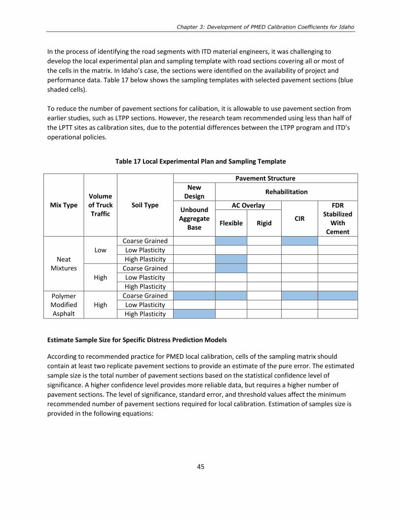
Chapter 3: Development of PMED Calibration Coefficients for Idaho
45
In the process of identifying the road segments with ITD material engineers, it was challenging to
develop the local experimental plan and sampling template with road sections covering all or most of
the cells in the matrix. In Idaho’s case, the sections were identified on the availability of project and
performance data. Table 17 below shows the sampling templates with selected pavement sections (blue
shaded cells).
To reduce the number of pavement sections for calibation, it is allowable to use pavement section from
earlier studies, such as LTPP sections. However, the research team recommended using less than half of
the LPTT sites as calibration sites, due to the potential differences between the LTPP program and ITD’s
operational policies.
Table 17 Local Experimental Plan and Sampling Template
Mix Type Volume of Truck Traffic
Soil Type
Pavement Structure
New Design
Rehabilitation
Unbound Aggregate
Base
AC Overlay
CIR
FDR Stabilized
With Cement
Flexible Rigid
Neat Mixtures
Low
Coarse Grained
Low Plasticity
High Plasticity
High
Coarse Grained
Low Plasticity
High Plasticity
Polymer Modified Asphalt
High
Coarse Grained
Low Plasticity
High Plasticity
Estimate Sample Size for Specific Distress Prediction Models
According to recommended practice for PMED local calibration, cells of the sampling matrix should
contain at least two replicate pavement sections to provide an estimate of the pure error. The estimated
sample size is the total number of pavement sections based on the statistical confidence level of
significance. A higher confidence level provides more reliable data, but requires a higher number of
pavement sections. The level of significance, standard error, and threshold values affect the minimum
recommended number of pavement sections required for local calibration. Estimation of samples size is
provided in the following equations:
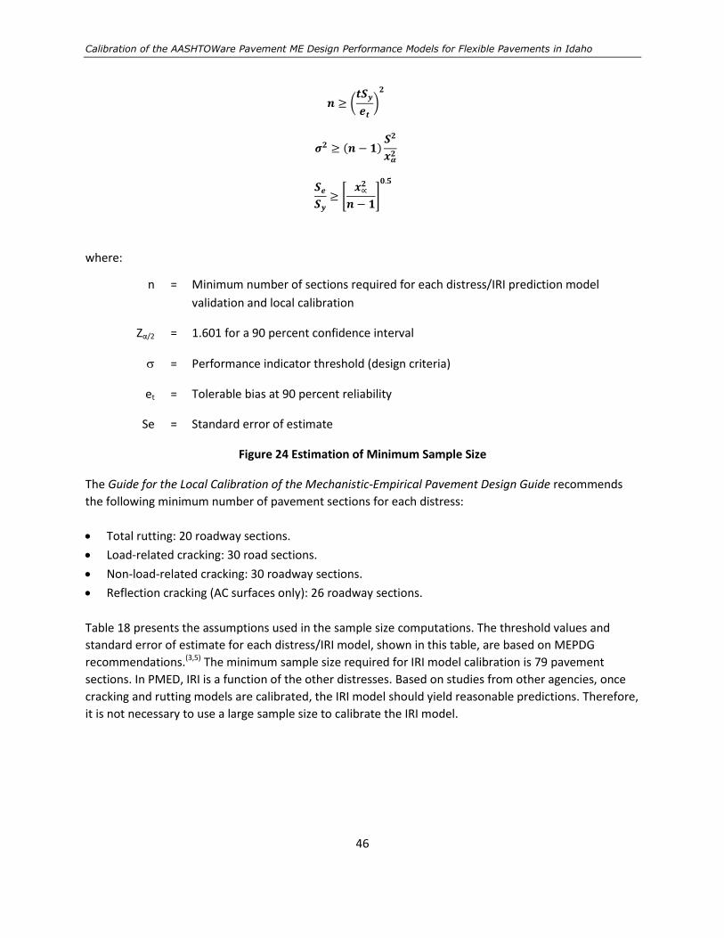
Calibration of the AASHTOWare Pavement ME Design Performance Models for Flexible Pavements in Idaho
46
𝒏 ≥ (𝒕𝑺𝒚
𝒆𝒕
)𝟐
𝝈𝟐 ≥ (𝒏 − 𝟏)𝑺𝟐
𝒙𝜶𝟐
𝑺𝒆
𝑺𝒚
≥ [𝒙∝
𝟐
𝒏 − 𝟏]
𝟎.𝟓
where:
n = Minimum number of sections required for each distress/IRI prediction model
validation and local calibration
Zα/2 = 1.601 for a 90 percent confidence interval
= Performance indicator threshold (design criteria)
et = Tolerable bias at 90 percent reliability
Se = Standard error of estimate
Figure 24 Estimation of Minimum Sample Size
The Guide for the Local Calibration of the Mechanistic-Empirical Pavement Design Guide recommends
the following minimum number of pavement sections for each distress:
Total rutting: 20 roadway sections.
Load-related cracking: 30 road sections.
Non-load-related cracking: 30 roadway sections.
Reflection cracking (AC surfaces only): 26 roadway sections.
Table 18 presents the assumptions used in the sample size computations. The threshold values and
standard error of estimate for each distress/IRI model, shown in this table, are based on MEPDG
recommendations.(3,5) The minimum sample size required for IRI model calibration is 79 pavement
sections. In PMED, IRI is a function of the other distresses. Based on studies from other agencies, once
cracking and rutting models are calibrated, the IRI model should yield reasonable predictions. Therefore,
it is not necessary to use a large sample size to calibrate the IRI model.
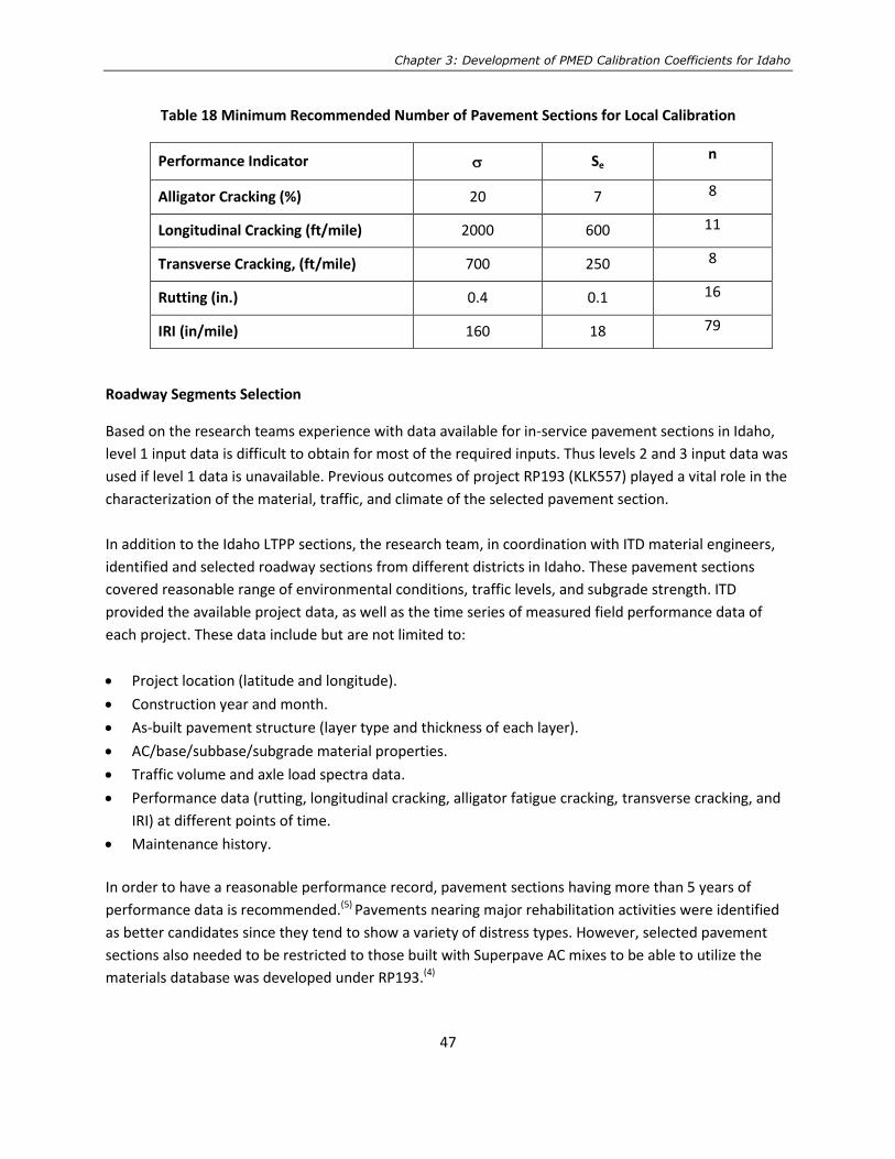
Chapter 3: Development of PMED Calibration Coefficients for Idaho
47
Table 18 Minimum Recommended Number of Pavement Sections for Local Calibration
Performance Indicator Se n
Alligator Cracking (%) 20 7 8
Longitudinal Cracking (ft/mile) 2000 600 11
Transverse Cracking, (ft/mile) 700 250 8
Rutting (in.) 0.4 0.1 16
IRI (in/mile) 160 18 79
Roadway Segments Selection
Based on the research teams experience with data available for in-service pavement sections in Idaho,
level 1 input data is difficult to obtain for most of the required inputs. Thus levels 2 and 3 input data was
used if level 1 data is unavailable. Previous outcomes of project RP193 (KLK557) played a vital role in the
characterization of the material, traffic, and climate of the selected pavement section.
In addition to the Idaho LTPP sections, the research team, in coordination with ITD material engineers,
identified and selected roadway sections from different districts in Idaho. These pavement sections
covered reasonable range of environmental conditions, traffic levels, and subgrade strength. ITD
provided the available project data, as well as the time series of measured field performance data of
each project. These data include but are not limited to:
Project location (latitude and longitude).
Construction year and month.
As-built pavement structure (layer type and thickness of each layer).
AC/base/subbase/subgrade material properties.
Traffic volume and axle load spectra data.
Performance data (rutting, longitudinal cracking, alligator fatigue cracking, transverse cracking, and
IRI) at different points of time.
Maintenance history.
In order to have a reasonable performance record, pavement sections having more than 5 years of
performance data is recommended.(5) Pavements nearing major rehabilitation activities were identified
as better candidates since they tend to show a variety of distress types. However, selected pavement
sections also needed to be restricted to those built with Superpave AC mixes to be able to utilize the
materials database was developed under RP193.(4)

Calibration of the AASHTOWare Pavement ME Design Performance Models for Flexible Pavements in Idaho
48
As described previously, ITD cracking data is collected in a format different from the PMED. Therefore, it
was difficult to quantify the cracking severity level. For this reason, the research team used the video log
files to redevelop the cracking data. The cracking observation was limited to a 3-year period for all
pavement sections based on the availability of the video log files. Having three data points for each
roadway section provides more reliable data than the severity level classification; moreover, each
roadway section has same number of performance observations. Statistically, it would not be good
practice to have some roadway segments with more observations than others, because segments that
having more observations would have a greater influence on the validation and calibration process than
the segments with less observations. Table 19 and Figure 25 shows the selected pavement sections and
geographical locations, respectively.
Table 19 List of the Roadway Segments Selected for Local Calibration
District # Construction
Year Route Beg MP End MP
D1
2008 US-95 403.5 408.75
2004 US-95 411.84 415.83
2002 US-95 415.5 421.3
2006 SH-3 76.822 84.201
2013 SH-3 103.15 111.38
2013 US-95 477.1 486.36
D2
2008 SH006 100 104.5
2004 SH008 0 1.76
2003 US-95 344 344.57
2003 US-95 366.59 373.03
2007 US-95 319.88 337.67
2008 SH003 5.00 8.5
2011 SH013 11.257 18.711
2010 SH013 18.68 25.378
2005 US-95 277.28 279.1
D3
2012 SH 55 113.9 115.9
2010 US 95 64.94 67.14
2011 US 95 0 16.7
2012 US 95 38.4 46.6
2011 SH 55 66.1 80.63
2010 SH 78 29.1 36.7
2010 SH 78 0 11.5
2011 SH 51 60 76.9
2011 SH 55 63.2 66.1
2011 SH 51 47.7 54.6
2011 SH 78 60 76
2012 SH 55 13.1 18
2012 US 20/26 0 1.58
2012 US 95 47.58 60.87

Chapter 3: Development of PMED Calibration Coefficients for Idaho
49
Table 19 List of the Roadway Segments Selected for Local Calibration (Cont.)
Figure 25 Geographical Locations of the Selected Road Segments for Local Calibration
District # Construction
Year Route Beg MP End MP
D3 2012 SH 16 0 13.392
2013 SH 52 14.4 30.42
D4 2000 SH 77 18.5 23
D5
2005 US91 JCT-15 JCT US-91
2011 SH34 Conda RD Blackfoot RV
2014 US30 328.6 330.7
D6 2012 US20 328.6 335.7
2011 US20 377.08 387.03

Calibration of the AASHTOWare Pavement ME Design Performance Models for Flexible Pavements in Idaho
50
Extract and Evaluate Distress Project Data
After selecting the roadway segments, the next step is to collect all data and identify any missing
information. The collected data for the calibration can be divided into two main categories, input data
(e.g., traffic, pavement structure, layer properties) and performance data. For AC pavements, PMED
performance criteria includes rutting, load-related cracking (alligator and longitudinal), thermal cracking
(transverse), reflective cracking in AC overlays, and IRI.
ITD only collects surface rut depth, however, PMED determines rutting in each pavement layer (AC,
base, and subgrade). Collecting rut depth for each individual layer is expensive, time consuming, since
trenches are needed to evaluate rutting at each layer, and requires lane closures which are disruptive to
the traveling public. Therefore, the research team used the simple approach to determine the rut depth
for each layer. This approach includes determining the percent of total rutting in each layer from the
PMED output and multiplying that percent by the total measured rutting.
Table 20 shows the types of asphalt and rigid pavement cracking reported by ITD. Each crack type
includes three severity levels; low, medium, and high. However, the PMED only predicts longitudinal
(top down fatigue cracking), transverse (thermal cracking), and alligator (bottom-up fatigue cracking).
Table 20 Asphalt and Rigid Pavement Cracking Types Collected in Idaho
Flexible (asphalt) cracking collected Rigid (concrete) cracking collected
Alligator Transverse Slab
Block Spalling
Edge Scaling
Transverse Meander
Longitudinal Faulting
Patching/Potholes Corner
Table 21 compares the current IDT distress report with those of the PMED.

Chapter 3: Development of PMED Calibration Coefficients for Idaho
51
Table 21 Comparison between ITD and PMED Flexible Pavement Distresses
Distress Type ITD PMED
Permanent deformation - total
pavement Total rut depth (inch) Rut depth (inch)
Permanent deformation - AC
only Not reported Rut depth (inch)
Bottom-up fatigue (alligator)
cracking
Light/moderate/heavy extent
Slight/moderate/heavy severity Area percentage
Thermal (transverse) cracking Light/moderate/heavy extent
Slight/moderate/heavy severity ft/mile
Top-down fatigue
(longitudinal) cracking
Light/moderate/heavy extent
Slight/moderate/heavy severity ft/mile
In order to use the historic ITD performance data, the research team first quantified distresses according
to the ITD pavement rating manual guide,(35,36) using the average or representative value for each
distress rating. Table 22 shows the cracking severity and extent per the ITD manual. Cracking is reported
as light, moderate, and heavy extent and slight, moderate, and heavy severity, which could be
reproduced by assigning an average cracking value for each rating. However, the level of accuracy was
very low, and the variability was high. It was also difficult to quantify the cracks based on the crack
rating and severity level, especially, when the roadway section has the same rating for different years.
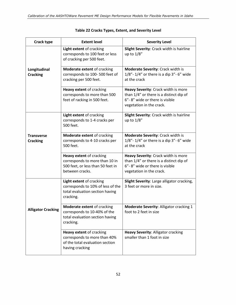
Calibration of the AASHTOWare Pavement ME Design Performance Models for Flexible Pavements in Idaho
52
Table 22 Cracks Types, Extent, and Severity Level
Crack type Extent level Severity Level
Longitudinal Cracking
Light extent of cracking corresponds to 100 feet or less of cracking per 500 feet.
Slight Severity: Crack width is hairline up to 1/8”
Moderate extent of cracking corresponds to 100- 500 feet of cracking per 500 feet.
Moderate Severity: Crack width is 1/8”- 1/4” or there is a dip 3”- 6” wide at the crack
Heavy extent of cracking corresponds to more than 500 feet of racking in 500 feet.
Heavy Severity: Crack width is more than 1/4” or there is a distinct dip of 6”- 8” wide or there is visible vegetation in the crack.
Transverse Cracking
Light extent of cracking corresponds to 1-4 cracks per 500 feet.
Slight Severity: Crack width is hairline up to 1/8”
Moderate extent of cracking corresponds to 4-10 cracks per 500 feet.
Moderate Severity: Crack width is 1/8”- 1/4” or there is a dip 3”- 6” wide at the crack
Heavy extent of cracking corresponds to more than 10 in 500 feet, or less than 50 feet in between cracks.
Heavy Severity: Crack width is more than 1/4” or there is a distinct dip of 6”- 8” wide or there is visible vegetation in the crack.
Alligator Cracking
Light extent of cracking corresponds to 10% of less of the total evaluation section having cracking.
Slight Severity: Large alligator cracking, 3 feet or more in size.
Moderate extent of cracking corresponds to 10-40% of the total evaluation section having cracking.
Moderate Severity: Alligator cracking 1 foot to 2 feet in size
Heavy extent of cracking corresponds to more than 40% of the total evaluation section having cracking
Heavy Severity: Alligator cracking smaller than 1 foot in size

Chapter 3: Development of PMED Calibration Coefficients for Idaho
53
As an alternative approach, the research team used the video log data files and analyze each photo
manually to collect the cracking data. Figure 26 shows an example of the photos from the video log.
Alligator Cracking (ft^2) Trans. Cracking (ft/mile) Long. Cracking (ft/mile)
Figure 26 Example of Extracted Images of the Video-Based Distress Data Collection
The cracking data observation was limited to a 3 year period (2014 to 2016) for all pavement section.
The procedure was to track each roadway section using PathView software provided by ITD, and
quantify the amount of alligator, longitudinal, and thermal cracking. Each photo has a dimension that
represent 13.6 ft. wide and 26.4 feet long. The alligator cracking was measured as an area in square feet,
and longitudinal and thermal cracking were measured in ft. using a measurement tool available in the
PathView software. Cracks were recorded for each photo. The data was tabulated for 200 photos,
representing 1-mile (Figure 27). Vendor software can analyze images automatically; however, it was not
available to the research team, and based on communications with the software vender, the automated
tool does not provide the accuracy level needed for PMED calibrated. For these reason, the research
team conduct crack measurement manually.

Calibration of the AASHTOWare Pavement ME Design Performance Models for Flexible Pavements in Idaho
54
Figure 27 Example of Data Sheet for Cracking Analysis Using PathView Video Images
ITD collects all other inputs, such as traffic, climate, and materials, in the same process as the PMED.
Conduct Field and Forensic Investigations
Since, the research team obtained the video log data for the selected road sections, there was sufficient
data to observe crack propagation over the three year period. However, for rutting, it was impossible to
determine if the rutting happened in the AC layer alone or in all layers of the roadway section. For this
reason, the research team conducted a field investigation on one heavily loaded roadway section, State
Highway 8, located in district two (SH008). This roadway section developed rut depths, and was one of
the best sections to conduct a forensic investigation. Figure 28 shows the roadway section plan and
trench locations.

Chapter 3: Development of PMED Calibration Coefficients for Idaho
55
Figure 28 Plan of SH008 Trench Locations
The AC layer rutting was less than the total rutting for all trenches. This concludes the measured rutting
happened in all layers. Which is in support of the assumption used to calculate rutting in each layer.
Figure 29 and 30 show a pavement cross section and rut measurements taken during the investigation.
Figure 29 Trench Side View

Calibration of the AASHTOWare Pavement ME Design Performance Models for Flexible Pavements in Idaho
56
Rut Depth (in.) Left Edge Left wheel
path
Center of
the lane
Right wheel
path Right Edge
Total rutting ( surface) 0 0.48,0.49 0 0.33, 0.28 0
AC layer thickness 4.8, 4.92,4.83 4.26,4.28, ,4.30 4.73,4.75,4.78 4.62,4.69,4.63 4.79,4.83,4.82
Base layer thickness 3.67 3.63 3.58 3.55 3.59
Subbase layer
thickness 17.3 16.5 16.5 16.5 16.5
Figure 30 Example of Trench Rut Depth Measurements on SH008
Assess Local Bias: Validation of Global Calibration Values to Local Conditions, Polices, and Materials
Bias is defined as consistent under or over prediction of distress/IRI and can be determined using
statistical methods. A significance level, α, of 0.05 or 5 percent, was assumed for all hypothesis testing
described explained:
Hypothesis 1: Perform a paired t-test to test:
i. H0: Mean measured distress/IRI = mean predicted distress/IRI.
ii. HA: Mean measured distress/IRI ≠ mean predicted distress/IRI.
If the hypothesis is accepted, local calibration is not required and the global calibration coeficients are
robust and produce accurate predictions of pavement distress. Rejecting the null hypothesis (p-value <
0.05) implies the measured and predicted PMED distress/IRI are from different populations. This
indicates that for the range of distress/IRI used in the analysis, the PMED results in biased predictions.
When the null hypothesis is rejected, adjustments need to be made to the calibration coefficients due to
the significant differences found between the predicted and measured performance. It will also be
necessary to determine which calibration coefficients are causing these differences so appropriate
adjustments can be made. A full factorial is not needed for local calibration, but replication within some
Base Layer
Subbase Layer
AC Layer

Chapter 3: Development of PMED Calibration Coefficients for Idaho
57
cells is needed when a partial or fractional factorial is used. The experimental plan and sampling matrix
is developed around the hypothesis that there is no significant bias and no error between the measured
and predicted performance.(3,5) Figure 31 shows an example of rutting and IRI distress indicators and the
null hypothesis test.
Figure 31 Distress Indictors (Rutting and IRI) with the Null Hypothesis Test
After collecting all the data for the selected pavement sections, the research team ran the PMED. Table
23 presents the statistical analysis of the selected roadway sections using the globally-calibrated
coefficients. As can be seen, distresses with a p-value less than 0.05 indicates significant difference
between the measured and predicted distress. Therefore, local calibration should be conducted to
reduce the bias and the sum of standard errors.
Table 23 Summary of Statistical Analysis of Predicted vs. Measured Distress Using the Global
Calibration Coefficients
Performance Indicator
N Bias
er(mean)
Standard Error (Se)
Sy Se/Sy R2, %
p-value (t-test)
Total Rutting (in)
113 -0.0686 0.093 0.034 2.783 3.7% <0.0001
Alligator Cracking (%)
101 -0.412 1.103 0.202 5.467 0.4% <0.0001
Longitudinal Cracking (ft/mile)
96 -455.87 841.047 63.193 13.309 28.65% <0.0001
Transverse Cracking (ft/mile)
118 63.559 207.160 197.325 1.050 1.95% <0.0001
IRI (in/mile)
128 -16.805 34.310 51.188 0.670 35% <0.0001

Calibration of the AASHTOWare Pavement ME Design Performance Models for Flexible Pavements in Idaho
58
Eliminate Local Bias of Distress and IRI Prediction Models
The cause of the local bias should be identified and removed in this step. Elimination of the bias should
consider traffic conditions, climate, and material characteristics. Performance prediction may be
improved by adjusting calibration coefficients, rerunning the PMED, and analyzing the results. Table 24
shows the recommended calibration coefficients that can be modified to eliminate bias.(5)
Table 24 Calibration Parameters to Adjust to Eliminate Bias(3,5)
Distress Eliminate Bias
Total Rutting AC and Unbound
Materials Layers Kr1, βs1, β r1
Load Related Cracking
Alligator Cracking C2, Kf1
Longitudinal Cracking C2, Kf1
Semi-Rigid Pavements C2, βc1
Non-Load Related
Cracking Transverse Cracking β f3
Roughness, IRI C4
Assess the Standard Error of the Estimate
After eliminating the bias, coefficient of determination (R2) and standard error of the estimate (SEE) are
computed using the developed local calibration coefficients to evaluate the new calibrated models
goodness of fit. The calibrated model’s R2 and SEE are compared to the PMED global calibration R2 and
SEE. Engineering judgment and diagnostic statistics can be used to determine the reasonableness of
goodness of fit. Models exhibiting a low R2 (i.e., less than 50 percent) or excessive SEE are deemed as
having a poor goodness of fit.
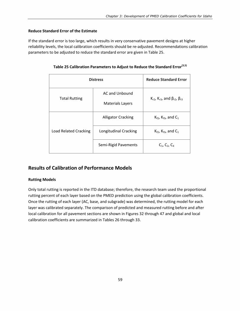
Chapter 3: Development of PMED Calibration Coefficients for Idaho
59
Reduce Standard Error of the Estimate
If the standard error is too large, which results in very conservative pavement designs at higher
reliability levels, the local calibration coefficients should be re-adjusted. Recommendations calibration
parameters to be adjusted to reduce the standard error are given in Table 25.
Table 25 Calibration Parameters to Adjust to Reduce the Standard Error(3,5)
Distress Reduce Standard Error
Total Rutting AC and Unbound
Materials Layers Kr2, Kr3, and βr2, βr3
Load Related Cracking
Alligator Cracking Kf2, Kf3, and C1
Longitudinal Cracking Kf2, Kf3, and C1
Semi-Rigid Pavements C1, C2, C4
Results of Calibration of Performance Models
Rutting Models
Only total rutting is reported in the ITD database; therefore, the research team used the proportional
rutting percent of each layer based on the PMED prediction using the global calibration coefficients.
Once the rutting of each layer (AC, base, and subgrade) was determined, the rutting model for each
layer was calibrated separately. The comparison of predicted and measured rutting before and after
local calibration for all pavement sections are shown in Figures 32 through 47 and global and local
calibration coefficients are summarized in Tables 26 through 33.

Calibration of the AASHTOWare Pavement ME Design Performance Models for Flexible Pavements in Idaho
60
Figure 32 Measured vs. Predicted AC Rutting Using Global Calibration Coefficients
Figure 33 Measured vs. Predicted AC Rutting Using Local Calibration Coefficients
Table 26 Calibration Coefficients for AC Layer Rutting
Calibration
Coefficients β1r β2r β3r N
Bias,
er(mean)
Standard
Error, Se Se/Sy R2, %
p-value
(Paired
t-test)
Global 1.00 1.00 1.00 113 -0.0293 0.040 1.707 29.5 6.79E-21
Local 3.00 1.00 0.661 113 -9E-05 0.021 0.888 47.8 0.132
0.00
0.05
0.10
0.15
0.20
0.25
0.30
0.35
0.40
0.00 0.05 0.10 0.15 0.20 0.25 0.30 0.35 0.40
Mea
sure
d R
utt
ing
(in
)
Predicted Rutting (in)
AC Rutting before Calibration Line of Equality
0.00
0.05
0.10
0.15
0.20
0.25
0.30
0.35
0.40
0.00 0.05 0.10 0.15 0.20 0.25 0.30 0.35 0.40
Me
asu
red
Ru
ttin
g (i
n)
Predicted Rutting (in)
Line of Equality AC Rutting after Calibration

Chapter 3: Development of PMED Calibration Coefficients for Idaho
61
Figure 34 Measured vs. Predicted Granular Base Rutting Using Global Calibration Coefficients
Figure 35 Measured vs. Predicted Granular Base Rutting Using Local Calibration Coefficients
Table 27 Calibration Coefficients for Base Layer Rutting
Calibration
Coefficient
β1s
(Coarse) N
Bias,
er(mean)
Standard
Error, Se Se/Sy R2, %
p-value
(Paired t-
test)
Global 1.00 113 -0.08955 0.120 2.571 23.9 7.62E-21
Local 0.53 113 -4.43E-05 0.046 0.987 48.5 0.482
0.000.020.040.060.080.100.120.140.160.180.20
0.00 0.02 0.04 0.06 0.08 0.10 0.12 0.14 0.16 0.18 0.20
Mea
sure
d R
utt
ing
(in
)
Predicted Rutting (in)
Base Rutting before Calibration Line of Equality
0.00
0.02
0.04
0.06
0.08
0.10
0.12
0.14
0.16
0.18
0.20
0.00 0.02 0.04 0.06 0.08 0.10 0.12 0.14 0.16 0.18 0.20
Me
asu
red
Ru
ttin
g (i
n)
Predicted Rutting (in)
Line of Equality Base Rutting after Calibration

Calibration of the AASHTOWare Pavement ME Design Performance Models for Flexible Pavements in Idaho
62
Figure 36 Measured vs. Predicted Subgrade Rutting Using Global Calibration Coefficients
Figure 37 Measured vs. Predicted Subgrade Rutting Using Local Calibration Coefficients
Table 28 Calibration Coefficients for Subgrade Rutting
Calibration
Coefficients
β1s
(Fine) N
Bias,
er(mean)
Standard
Error, Se Se/Sy R2, %
p-value
(Paired t-
test)
Global 1.00 113 -0.18745 0.240 2.973 22.9 5.93E-22
Local 0.477 113 -0.00379 0.096 1.183 47.4 0.496
0.000.050.100.150.200.250.300.350.400.450.50
0.00 0.05 0.10 0.15 0.20 0.25 0.30 0.35 0.40 0.45 0.50
Mea
sure
d R
utt
ing
(in
)
Predicted Rutting (in)
Subgrade Rutting before Calibration Line of Equality
0.000.050.100.150.200.250.300.350.400.450.50
0.00 0.05 0.10 0.15 0.20 0.25 0.30 0.35 0.40 0.45 0.50
Me
asu
red
Ru
ttin
g (i
n)
Predicted Rutting (in)
Line of Equality Subgrade Rutting after Calibration

Chapter 3: Development of PMED Calibration Coefficients for Idaho
63
Figure 38 Measured vs. Predicted Total Rutting Using Global Calibration Coefficients
Figure 39 Measured vs. Predicted Total Rutting Using Local Calibration Coefficients
Table 29 Calibration Coefficients for Rutting
Calibration
Coefficient β1r β2r β3r
β1s
(Coarse)
β1s
(Fine) N
Bias,
er(mean)
Standard
Error, Se Se/Sy R
2, %
p-value
(Paired t-
test)
Global 1.00 1.00 1.00 1.00 1.00 113 -0.06858 0.093 2.783 3.7 8.27E-25
Local 3.000 1.000 0.661 0.530 0.477 113 -0.00365 0.035 1.034 17.6 0.338
0
0.1
0.2
0.3
0.4
0.5
0.6
0.7
0.8
0 0.1 0.2 0.3 0.4 0.5 0.6 0.7 0.8
Mea
sure
d R
utt
ing
(in
)
Predicted Rutting (in)
Total Rutting before Calibration Line of Equality
0
0.1
0.2
0.3
0.4
0.5
0.6
0.7
0.8
0 0.1 0.2 0.3 0.4 0.5 0.6 0.7 0.8
Me
asu
red
Ru
ttin
g (i
n)
Predicted Rutting (in)
Line of Equality Total Rutting After Calibration

Calibration of the AASHTOWare Pavement ME Design Performance Models for Flexible Pavements in Idaho
64
Longitudinal (Top-Down) Cracking Model
Figure 24 shows a comparison of measured and predicted longitudinal cracking using the globally-
calibrated coefficients. The globally-calibrated model over-predicts the extent of longitudinal cracking.
The researchers conducted several iterations and were unable to calibrate the model. The locally-
calibrated coefficients that result in a lower bias are shown in Table 30. However, this improvement is
not statistically significant. Some agencies have reported the same conclusion and recommend using the
longitudinal crack prediction for informational and experimental purposes, and not for design at this
time.(22,24,32) The longitudinal cracking prediction model is under development in NCHRP Project 1-52, A
Mechanistic-Empirical Model for Top-Down Cracking of Asphalt Pavement Layers.
Figure 40 Measured vs. Predicted Longitudinal Cracking Using Global Calibration Coefficients
Figure 41 Measured vs. Predicted Longitudinal Cracking Using Local Calibration Coefficients
0
500
1000
1500
2000
2500
3000
3500
4000
0 500 1000 1500 2000 2500 3000 3500 4000
Me
asu
red
Lo
ng.
Cra
ckin
g (f
t/m
ile
)
Predicted Long. Cracking (ft/mile)
Longitudinal Cracking before calibration Line of Equality
0
500
1000
1500
2000
2500
3000
3500
4000
0 500 1000 1500 2000 2500 3000 3500 4000
Mea
sure
d L
on
g. C
rack
ing
(ft/
mile
)
Predicted Long. Cracking (ft/mile)
Line of Equality Longitudinal Cracking after Calibration

Chapter 3: Development of PMED Calibration Coefficients for Idaho
65
Table 30 Calibration Coefficients for Longitudinal Cracking
Calibration
Coefficient Βf1 Βf2 Βf3 C1 C2 N
Bias,
er(mean)
Standard
Error, Se Se/Sy R
2, %
p-value
(Paired t-
test)
Global 1.00 1.00 1.00 7.00 3.50 123 -634.56 1136.54 2.57 2.27 8.05E-12
Local 1.00 1.00 1.00 4.533 0.229 123 -602.78 1047.86 2.37 15.70 1.40E-12
Alligator (Bottom-Up) Cracking Model
Figure 26 and 27 compare the AC alligator cracking measurements and corresponding predictions
obtained using the nationally calibrated model, statistically there is no significant difference between
predicted and measured alligator cracking. The research team was able to improve the model further by
reducing the error. Table 31 shows the developed calibration coefficients.
Thermal (Transverse) Cracking Model
Previous studies reported that little or no thermal cracking was predicted when using the appropriate
PG binder for local climate conditions. As seen in Figure 28, the globally-calibrated thermal cracking
model under predicts thermal cracking. Modification of calibration coefficients could not provide
significant changes in PMED model predictions. In PMED v2.3.1, there is no input cell to change the
thermal cracking model local calibration coefficient (βt1). Therefore, the research team adjusted the K
value from the global calibration to compensate for the βt1 in thermal cracking model. Table 32
presents the statistical analysis of thermal cracking model using globally and locally coefficients.
International Roughness Index Model
Figure 30 and 31 compares the predicted and measured IRI values using the global- and local calibrated
coefficients, respectively. Both IRI models provide good estimation to field measurements. Further
modification to the IRI model calibration coefficients were considered to improve prediction are shown
in Table 33.
Interpretation of results and deciding on adequacy of the calibration coefficients is the last step in the
calibration process. The standard error of the estimate for each distress and IRI prediction model should
be evaluated to determine the impact on the resulting designs at different reliability levels. If the local
calibration coefficients produce reasonable designs, the developed calibration coefficients can be
implemented. If not, the calibration coefficients should be re-adjusted.
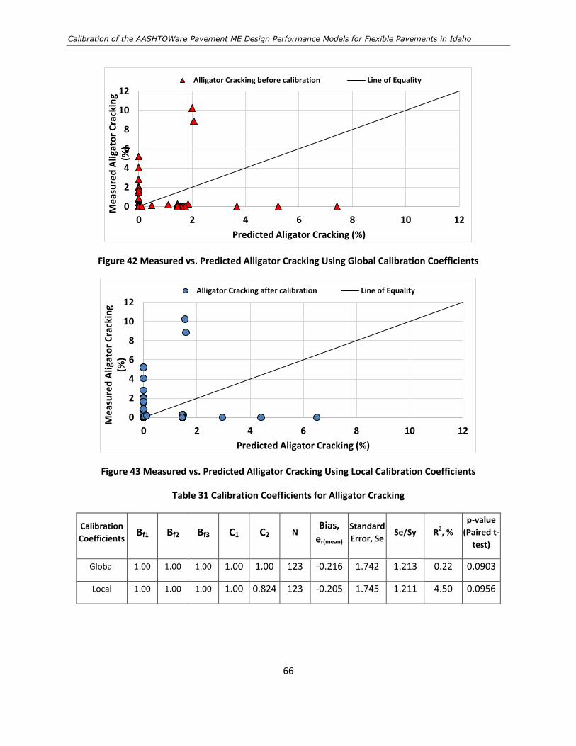
Calibration of the AASHTOWare Pavement ME Design Performance Models for Flexible Pavements in Idaho
66
Figure 42 Measured vs. Predicted Alligator Cracking Using Global Calibration Coefficients
Figure 43 Measured vs. Predicted Alligator Cracking Using Local Calibration Coefficients
Table 31 Calibration Coefficients for Alligator Cracking
Calibration
Coefficients Βf1 Βf2 Βf3 C1 C2 N
Bias,
er(mean)
Standard
Error, Se Se/Sy R
2, %
p-value
(Paired t-
test)
Global 1.00 1.00 1.00 1.00 1.00 123 -0.216 1.742 1.213 0.22 0.0903
Local 1.00 1.00 1.00 1.00 0.824 123 -0.205 1.745 1.211 4.50 0.0956
0
2
4
6
8
10
12
0 2 4 6 8 10 12
Mea
sure
d A
ligat
or
Cra
ckin
g (%
)
Predicted Aligator Cracking (%)
Alligator Cracking before calibration Line of Equality
0
2
4
6
8
10
12
0 2 4 6 8 10 12
Me
asu
red
Alig
ato
r C
rack
ing
(%)
Predicted Aligator Cracking (%)
Alligator Cracking after calibration Line of Equality

Chapter 3: Development of PMED Calibration Coefficients for Idaho
67
Figure 44 Measured vs. Predicted Transverse Cracking Using Global Calibration Coefficients
Figure 45 Measured vs. Predicted Transverse Cracking Using Local Calibration Coefficients
Table 32 Calibration Coefficients for Thermal Cracking
Calibration
Coefficients K1,2,3 N
Bias,
er(mean)
Standard
Error, Se Se/Sy R
2, %
p-value
(Paired t-
test)
Global 1.5,0.5,1.5 118 63.559 207.160 1.050 1.95% 0.000495
Local 2.169,0.835,2.169 118 21.9495 155.251 0.787 59.81% 0.116
0100200300400500600700800900
1000
0 100 200 300 400 500 600 700 800 900 1000
Mea
sure
d T
her
mal
Cra
ckin
g (f
t/m
ile)
Predicted Thermal Cracking (ft/mile)
Thermal Cracking before calibration Line of Equality
0100200300400500600700800900
1000
0 100 200 300 400 500 600 700 800 900 1000
Me
asu
red
Th
erm
al C
rack
ing
(ft/
mil
e)
Predicted Thermal Cracking (ft/mile)
Line of Equality Thermal Cracking after calibration

Calibration of the AASHTOWare Pavement ME Design Performance Models for Flexible Pavements in Idaho
68
Figure 46 Measured vs. Predicted IRI Using Global Calibration Coefficients
Figure 47 Measured vs. Predicted IRI using Local Calibration Coefficients
Table 33 Calibration Coefficients for IRI
Calibration
Coefficients C1 C2 C3 C4 N
Bias,
er(mean)
Standard
Error, Se Se/Sy R
2, %
p-value
(Paired t-
test)
Global 40 0.40 0.008 0.015 128 -16.805 34.310 0.670 0.35% 5.37E-07
Local 35 0.35 0.008 0.010 128 -8.0169 28.472 0.556 2.20% 0.0642
0
50
100
150
200
250
300
0 50 100 150 200 250 300
Mea
sure
d IR
I (in
./m
ile)
Predicted IRI (in./mile)
IRI before calibration Line of Equality
0
50
100
150
200
250
300
0 50 100 150 200 250 300
Me
asu
red
IRI (
in./
mil
e)
Predicted IRI (in./mile)
Line of Equality IRI after calibration

Chapter 4: Validation of the Developed Calibration Coefficients
69
Chapter 4
Validation of the Developed Calibration Coefficients
The validation process is essential to illustrate that the calibrated models produce accurate predictions
of pavement deterioration in the field. Validation usually requires an additional and independent set of
pavement sections to confirm the calibration results. Successful model validation requires the bias and
precision statistics of the validation data set to be similar to those obtained from the local calibration
data set. Typically, two approaches are utilized to improve the accuracy of the predication model; the
traditional split-sample approach and an alternative jack-knifing approach for small sample sizes.
The split sample approach is usually employed in the statistical analysis. With an 80/20 split, 80 percent
of the randomly chosen data is used during local calibration, while the remaining 20 percent used for
validation. The lack of proper model validation is the most common mistake during model development,
often resulting in misleading results. When all the available data are used for local calibration, the
resulting goodness-of fit statistic only describes the model accuracy for the calibration data set, which
may not indicate prediction accuracy for the full population. The split-sample testing for model
validation solves this problem.
However, the traditional split-sample method has its limitations when it comes to small sample sizes
(defined as a partial factorial with less than 25 percent of the cells filled with a project but without
replication). Thus, the Jack-Knifing procedure is used as an alternative to the traditional approach to
analyze small sample sizes. From the literature review, the only agency that used the Jack-Knifing
method was Montana.
In this study, the calibrated models were validated using the split sample method. This was done by
running the PMED on the remaining pavement sections that were not included in the local calibration
process. Figures 48 through 55 show a comparison between the predicted and measured distresses. It is
observed that the local calibration considerably reduced the difference between predicted and
measured distresses/IRI as demonstrated by the statistical analysis shown in Tables 34 through 41.

Calibration of the AASHTOWare Pavement ME Design Performance Models for Flexible Pavements in Idaho
70
Figure 48 Measured vs. Predicted AC Using Local Calibration Coefficients
Table 34 Local Calibration Coefficients for AC Rutting
β1r β2r β3r N Bias,
er(mean)
Standard
Error, Se Se/Sy R2, %
p-value
(Paired
t-test)
3.000 1.000 0.661 26 -0.001 0.010 0.658 76.5 0.010
Figure 49 Measured vs. Predicted Base Layer Rutting Using Local Calibration Coefficients
0.00
0.05
0.10
0.15
0.20
0.25
0.30
0.35
0.40
0.00 0.05 0.10 0.15 0.20 0.25 0.30 0.35 0.40
Mea
sure
d R
utt
ing
(in
)
Predicted Rutting (in)
Line of Equality AC Rutting after Calibration
0.00
0.02
0.04
0.06
0.08
0.10
0.12
0.14
0.16
0.18
0.20
0.00 0.02 0.04 0.06 0.08 0.10 0.12 0.14 0.16 0.18 0.20
Mea
sure
d R
utt
ing
(in
)
Predicted Rutting (in)
Line of Equality Base Rutting after Calibration
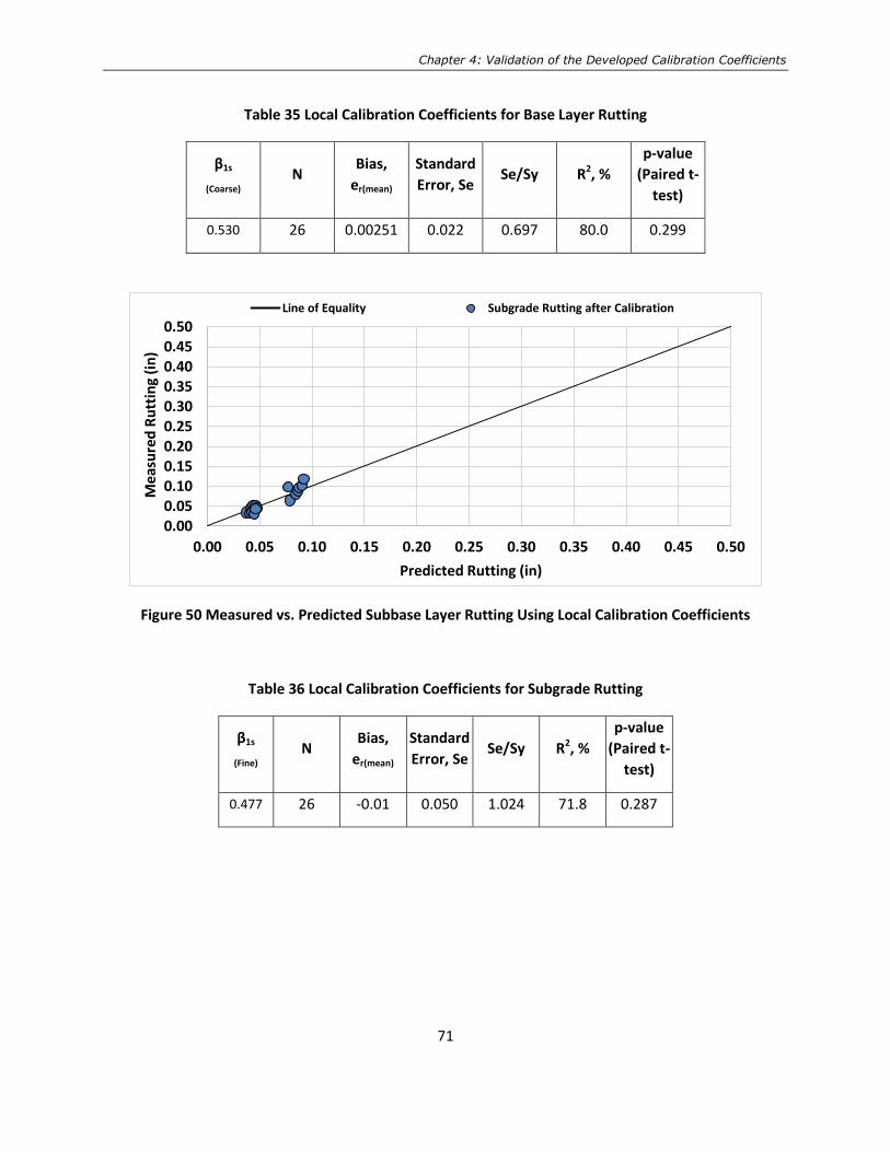
Chapter 4: Validation of the Developed Calibration Coefficients
71
Table 35 Local Calibration Coefficients for Base Layer Rutting
β1s
(Coarse) N
Bias,
er(mean)
Standard
Error, Se Se/Sy R2, %
p-value
(Paired t-
test)
0.530 26 0.00251 0.022 0.697 80.0 0.299
Figure 50 Measured vs. Predicted Subbase Layer Rutting Using Local Calibration Coefficients
Table 36 Local Calibration Coefficients for Subgrade Rutting
β1s
(Fine) N
Bias,
er(mean)
Standard
Error, Se Se/Sy R2, %
p-value
(Paired t-
test)
0.477 26 -0.01 0.050 1.024 71.8 0.287
0.000.050.100.150.200.250.300.350.400.450.50
0.00 0.05 0.10 0.15 0.20 0.25 0.30 0.35 0.40 0.45 0.50
Me
asu
red
Ru
ttin
g (i
n)
Predicted Rutting (in)
Line of Equality Subgrade Rutting after Calibration

Calibration of the AASHTOWare Pavement ME Design Performance Models for Flexible Pavements in Idaho
72
Figure 51 Measured vs. Predicted Total Rutting Using Local Calibration Coefficients
Table 37 Local Calibration Coefficients for Total Rutting
β1r β2r β3r β1s
(Coarse)
β1s
(Fine) N
Bias,
er(mean)
Standard
Error, Se Se/Sy R
2, %
p-value
(Paired t-
test)
3.000 1.000 0.661 0.530 0.477 26 -0.0114 0.026 0.942 32.8 0.157
Figure 52 Measured vs. Predicted Alligator Cracking Using Local Calibration Coefficients
0
0.1
0.2
0.3
0.4
0.5
0.6
0.7
0.8
0 0.1 0.2 0.3 0.4 0.5 0.6 0.7 0.8
Mea
sure
d R
utt
ing
(in
)
Predicted Rutting (in)
Line of Equality Total Rutting After Calibration
0
0.2
0.4
0.6
0.8
1
1.2
1.4
1.6
1.8
2
0 0.2 0.4 0.6 0.8 1 1.2 1.4 1.6 1.8 2
Mea
sure
d A
ligat
or
Cra
ckin
g (%
)
Predicted Aligator Cracking (%)
Alligator Cracking after calibration Linear (Line of Equality)
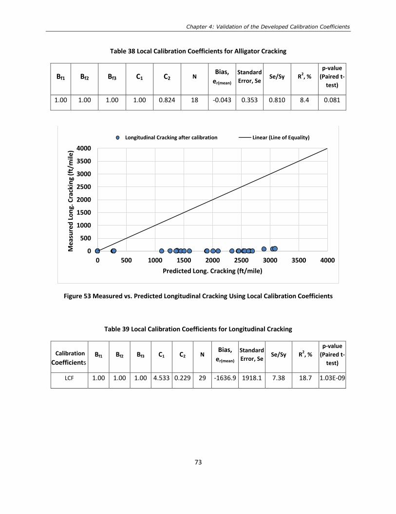
Chapter 4: Validation of the Developed Calibration Coefficients
73
Table 38 Local Calibration Coefficients for Alligator Cracking
Βf1 Βf2 Βf3 C1 C2 N Bias,
er(mean)
Standard
Error, Se Se/Sy R
2, %
p-value
(Paired t-
test)
1.00 1.00 1.00 1.00 0.824 18 -0.043 0.353 0.810 8.4 0.081
Figure 53 Measured vs. Predicted Longitudinal Cracking Using Local Calibration Coefficients
Table 39 Local Calibration Coefficients for Longitudinal Cracking
Calibration
Coefficients Βf1 Βf2 Βf3 C1 C2 N
Bias,
er(mean)
Standard
Error, Se Se/Sy R
2, %
p-value
(Paired t-
test)
LCF 1.00 1.00 1.00 4.533 0.229 29 -1636.9 1918.1 7.38 18.7 1.03E-09
0
500
1000
1500
2000
2500
3000
3500
4000
0 500 1000 1500 2000 2500 3000 3500 4000
Me
asu
red
Lo
ng.
Cra
ckin
g (f
t/m
ile)
Predicted Long. Cracking (ft/mile)
Longitudinal Cracking after calibration Linear (Line of Equality)

Calibration of the AASHTOWare Pavement ME Design Performance Models for Flexible Pavements in Idaho
74
Figure 54 Measured vs. Predicted Thermal Cracking Using Local Calibration Coefficients
Table 40 Local Calibration Coefficients for Thermal Cracking
K1,2,3 N Bias,
er(mean)
Standard
Error, Se Se/Sy R
2, %
p-value
(Paired t-
test)
2.169,0.835,2.169 26 -10.493 70.679 1.331 0.77 0.229
Figure 55 Measured vs. Predicted IRI Using Local Calibration Coefficients
0
20
40
60
80
100
120
140
160
180
200
0 20 40 60 80 100 120 140 160 180 200
Mea
sure
d T
her
mal
Cra
ckin
g (f
t/m
ile)
Predicted Thermal Cracking (ft/mile)
Thermal Cracking after Calibration Line of Equality
0
50
100
150
200
250
0 50 100 150 200 250
Mea
sure
d IR
I (in
./m
ile
)
Predicted IRI (in./mile)
IRI after calibration Line of Equality

Chapter 4: Validation of the Developed Calibration Coefficients
75
Table 41 Calibration Coefficients for IRI
C1 C2 C3 C4 N Bias, er
(mean) Standard
Error, Se Se/Sy R
2, %
p-value
(Paired t-
test)
35 0.35 0.008 0.010 27 -5.439 31.439 0.6807 56.92 0.189

Calibration of the AASHTOWare Pavement ME Design Performance Models for Flexible Pavements in Idaho
76

Chapter 5: Summary, Conclusions, and Recommendations
77
Chapter 5
Summary, Conclusions, and Recommendations
Summary
This research aims to improve the accuracy of PMED performance predictions for Idaho pavements
through local calibration. A total of 32 Asphalt Concrete pavement sections from different ITD districts
were selected. The required PMED inputs for the selected pavement sections were primarily collected
from material testing records, ITD phase reports, Job Mix Formula reports and the previous research
report (RP193) as well as material testing results of creep compliance and indirect tensile testing
performed in this project under Task4. A database of historical performance data for the selected
pavement sections was prepared using data contained in the ITD Transportation Asset Management
System (TAMS). The accuracy of the globally-calibrated PMED performance prediction models to Idaho
conditions was evaluated. A statistical evaluation indicated that the global calibration coefficients did
not accurately reflect Idaho in-service pavement performance. Therefore, a local calibration was
conducted using a trial and error method, with multiple iterations, to improve the accuracy of model
predictions.
The local calibration coefficients identified through this study are summarized in Table 42.
Table 42 Summary of Calibration Coefficients Before and After Local Calibration
Performance Model Coefficients before
Calibration
Coefficients after Calibration
Alligator Cracking
βf1
= 1.00 βf1
= 1.00
βf2
= 1.00 βf2
= 1.00
βf3
= 1.00 βf3
= 1.00
C1= 1.00 C1= 1.00
C2= 1.00 C2= 0.824
Longitudinal Cracking
βf1
= 1.00 βf1
= 1.00
βf2
= 1.00 βf2
= 1.00
βf3
= 1.00 βf3
= 1.00
C1= 7.00 C1= 4.533
C2 = 3.50 C2 = 0.229
Thermal Cracking
K1 = 1.50 K1 = 2.169
K2 = 0.50 K2 = 0.835
K3 = 1.50 K3 = 2.169
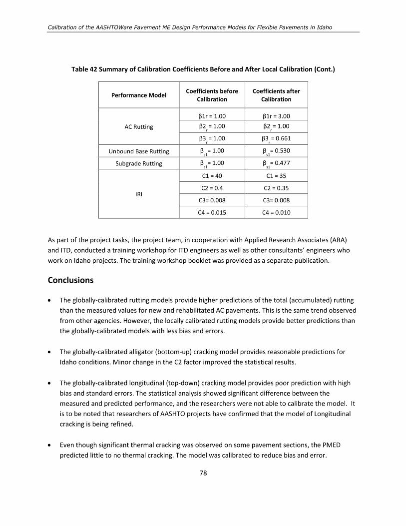
Calibration of the AASHTOWare Pavement ME Design Performance Models for Flexible Pavements in Idaho
78
Table 42 Summary of Calibration Coefficients Before and After Local Calibration (Cont.)
Performance Model Coefficients before
Calibration
Coefficients after Calibration
AC Rutting
β1r = 1.00 β1r = 3.00
β2r = 1.00 β2
r = 1.00
β3r = 1.00 β3
r = 0.661
Unbound Base Rutting βs1
= 1.00 βs1
= 0.530
Subgrade Rutting βs1
= 1.00 βs1
= 0.477
IRI
C1 = 40 C1 = 35
C2 = 0.4 C2 = 0.35
C3= 0.008 C3= 0.008
C4 = 0.015 C4 = 0.010
As part of the project tasks, the project team, in cooperation with Applied Research Associates (ARA)
and ITD, conducted a training workshop for ITD engineers as well as other consultants’ engineers who
work on Idaho projects. The training workshop booklet was provided as a separate publication.
Conclusions
The globally-calibrated rutting models provide higher predictions of the total (accumulated) rutting
than the measured values for new and rehabilitated AC pavements. This is the same trend observed
from other agencies. However, the locally calibrated rutting models provide better predictions than
the globally-calibrated models with less bias and errors.
The globally-calibrated alligator (bottom-up) cracking model provides reasonable predictions for
Idaho conditions. Minor change in the C2 factor improved the statistical results.
The globally-calibrated longitudinal (top-down) cracking model provides poor prediction with high
bias and standard errors. The statistical analysis showed significant difference between the
measured and predicted performance, and the researchers were not able to calibrate the model. It
is to be noted that researchers of AASHTO projects have confirmed that the model of Longitudinal
cracking is being refined.
Even though significant thermal cracking was observed on some pavement sections, the PMED
predicted little to no thermal cracking. The model was calibrated to reduce bias and error.

Chapter 5: Summary, Conclusions, and Recommendations
79
Good agreement is observed between predicted and measured IRI using the global calibration
coefficients. More refinement to the calibration coefficients was conducted to reduce the error.
ITD doesn’t differentiate between the fatigue and reflective cracking during the pavement condition
survey. Therefore, there was insufficient data to calibrate the reflective cracking model.
The semi-rigid fatigue cracking model was not calibrated in this study due to the lack of observed
fatigue cracking. None of the selected pavement sections for local calibration included AC over JPCP.
Some selected pavement sections included a cement treated base; however, no fatigue cracking
was observed in the field. As recommended in the Idaho PMED User Guide, all cement treated bases
were simulated in the PMED as non-stabilized base. For those reasons, the research team was
unable to calibrate the semi-rigid fatigue cracking model.
Recommendations
The calibration of the performance models is a continual process. Users need to allow reasonable
bias between model prediction and field performance. The final design should fall within a
reasonable range of expected values.
Ongoing and future work that examines and assesses PMED models and the software function
should continue to be monitored. The developed performance database for the selected pavement
sections should be updated with additional years of performance data to improve the accuracy of
the model prediction.
The PMED longitudinal cracking model should only be used for experimental/informational purposes,
until current model improvements are completed, validated, and local calibrated, if needed. The
longitudinal cracking model is currently undergoing refinement as part of NCHRP Project 1-52.
Some of the challenges identified in this study were the lack of observed distresses, limited ranges
of distress values, and pavement service life. There were limited observation of alligator and
longitudinal cracking in the selected pavement sections. Therefore, the research team recommends
continued monitoring of these pavement sections until the next major rehabilitation activity. At that
time, the alligator and longitudinal cracking models should be recalibrated.
ITD, through preventive maintenance, applies seal coats to many major pavement sections. Such an
application affects the observation of the distresses in the field, which may not necessary reflect the
real performance of these sections. The research team identified two sections where seal coats
were applied. These pavement sections should be excluded from any future calibration efforts.

Calibration of the AASHTOWare Pavement ME Design Performance Models for Flexible Pavements in Idaho
80
The PMED National Users Group, in their last meeting, discussed the tools to be added to the
software, including the potential for tool to assist with local calibration. The local calibration tool is
intended to “automate” the calibration process for reducing bias and error. Such a tool will require a
database containing roadway section and performance data. The database developed in this study
will play a vital role in providing accurate and precise data for future flexible pavement performance
model validation and calibration. The database should be continually updated and maintained to
support future PMED model calibration (or recalibration) efforts.

References
81
References
1. American Association of State Highways and Transportation Officials. AASHTO Guide for Design of
Pavement Structures. American Association of State Highways and Transportation Officials,
Washington, DC. 1993.
2. Applied Research Associates. Guide for the Mechanistic-Empirical Design of New & Rehabilitated
Pavement Structures. NCHRP Project 1-37A. Transportation Research Board, Washington, DC. 2004.
3. American Association of State Highway and Transportation Officials. Guide for the Local Calibration
of the Mechanistic-Empirical Pavement Design Guide. American Association of State Highway and
Transportation Officials, Washington, DC. 2010.
4. Bayomy, F., S. El-Badawy, and A. Awed. Implementation of the MEPDG for Flexible Pavements in
Idaho. RP193. Idaho Transportation Department, Boise, ID. 2012.
5. Mallela, J., H. Von Quintus, M. Darter, and B. Bhattacharya. Road Map for Implementing The
AASHTO Pavement ME Design Software for the Idaho Transportation Department. RP211A. Idaho
Transportation Department, Boise, ID. 2014.
6. Mallela, J., Glover, L., B. Bhattacharya, M. Darter, and H. Von Quintus, Idaho AASHTOWare
Pavement ME Design User’s Guide Version 1.1. RP211B. Idaho Transportation Department, Boise, ID.
2014.
7. Transportation Research Board. Facilitating the Implementation of the Guide for the Design of New
and Rehabilitated Pavement Structures, National Cooperative Highway Research Program 1-40.
Washington, DC: Transportation Research Board, National Research Council. Last Accessed
December 18, 2014.
8. Transportation Research Board. Jackknife Testing—An Experimental Approach to Refine Model
Calibration and Validation. Research Results Digest 283. Transportation Research Board,
Washington, DC. 2003.
9. Transportation Research Board. Refining the Calibration and Validation of Hot Mix Asphalt
Performance Models: An Experimental Plan and Database. Research Results Digest 284.
Transportation Research Board, Washington, DC. 2003.
10. American Association of State Highway and Transportation Officials. Mechanistic-Empirical
Pavement Design Guide: A Manual of Practice. Interim Edition. American Association of State
Highway and Transportation Officials, Washington, DC. 2008.

Calibration of the AASHTOWare Pavement ME Design Performance Models for Flexible Pavements in Idaho
82
11. American Association of State Highway and Transportation Officials. Mechanistic-Empirical
Pavement Design Guide. A Manual of Practice. American Association of State Highway and
Transportation Officials, Washington, DC. 2015.
12. Applied Pavement Technology. AASHTO Pavement ME User Group, Technical Report: First Annual
Meeting – Indianapolis, IN Dec 14-15, 2016. Federal Highway Administration, Washington, DC. 2017.
13. Witczak, M. W. Development of Performance Related Specifications for Asphalt Pavements in the
State of Arizona. Final Report 402-2. Arizona Department of Transportation, Phoenix, AZ. 2008.
http://www.azdot.gov/TPD/ATRC/Publications/project_reports/PDF/AZ402-2.pdf (Accessed in
February 2017).
14. Souliman, M. Calibration of the AASHTO MEPDG for Flexible Pavements for Arizona Conditions.
Master’s Thesis. Arizona State University, Tempe, AZ. 2009.
15. Lu, Q., Y. Zhang, and J. T. Harvey. “Estimation of Truck Traffic Inputs for Mechanistic-Empirical
Pavement Design in California,” Transportation Research Record No. 2095. Transportation Research
Board, Washington, DC. 2009.
16. Von Quintus, H. L. and J. S. Moulthrop. Mechanistic-Empirical Pavement Design Guide Flexible
Pavement Performance Prediction Models for Montana: Volume I - Executive Research Summary.
FHWA/MT-07-008/8158-1 Final Report. Montana Department of Transportation, Helena, MT. 2007.
http://www.archive.org/details/664B4642-A369-476C-BB5E-6196988FC74E (Accessed in January
2016).
17. Von Quintus, H. L. and J. S. Moulthrop. Mechanistic-Empirical Pavement Design Guide Flexible
Pavement Performance Prediction Models for Montana: Volume II - Reference Manual. Helena, MT:
Montana Department of Transportation, FHWA/MT-07-008/8158-1 Final Report, 2007.
http://www.archive.org/details/664B4642-A369-476C-BB5E-6196988FC74E, (Accessed in January
2016.
18. Von Quintus, H. L. and J. S. Moulthrop. Mechanistic-Empirical Pavement Design Guide Flexible
Pavement Performance Prediction Models for Montana: Volume III - Field Guide. Helena, MT:
Montana Department of Transportation, FHWA/MT-07-008/8158-1 Final Report, 2007.
http://www.archive.org/details/664B4642-A369-476C-BB5E-6196988FC74E, (Accessed in January
2016.
19. Karakouzian, M., Characterization of Unbound Materials (Soils/Aggregates) for Mechanistic
Empirical Pavement Design Guide (MEPDG). Report No. 361-16-803, Nevada Department of
Transportation, Carson, NV, 2018.
20. Nabhan, P., Calibration of the AASHTO MEPDG for Flexible Pavements to Fit Nevada’s
Conditions. Reno, NV: University of Nevada, Master’s Thesis, 2015.
References
83
21. Williams, R. C. and R. Shaidur. Mechanistic-Empirical Pavement Design Guide Calibration for Pavement Rehabilitation. 2013. Oregon Department of Transportation, Salem, OR. Retrieved from http://hdl.handle.net/2060/19650075465.
22. Darter, M., L. Titus-Glover, and H. Von Quintus. Implementation of the Mechanistic-Empirical
Pavement Design Guide in Utah: Validation, Calibration, and Development of the UDOT MEPDG
User’s Guide. Report No. UT-09.11. Utah Department of Transportation, Salt Lake City, UT. 2009.
http://utah.ptfs.com/awweb/main.jsp?flag=browse&smd=1&awdid=1 (Accesses in January 2016).
23. Li, J., L. Pierce, and J. Uhlmeyer. “Calibration of Flexible Pavement in Mechanistic-Empirical
Pavement Design Guide for Washington State.” Transportation Research Record 2095.
Transportation Research Board, Washington DC. 2009.
24. Ng, K. W., H. L. Von Quintus, K. Ksaibati, D. Hellrung, and Z. Hutson. Characterization of Material
Properties for Mechanistic-Empirical Pavement Design in Wyoming. Wyoming Department of
Transportation, Cheyenne, WY. 2013.
25. Hutson, Z., K. Ng, and K. Ksaibati. “Implementation in Wyoming through Comprehensive Testing
Program and Wyoming MEPDG Database.” 95th Annual TRB Meeting. Transportation Research
Board, Washington, DC. 2016.
26. Federal Highway Administration. Local Calibration of the MEPDG Using Pavement Management
Systems. HIF-11-026. Federal Highway Administration. Washington, DC, 2010
27. Von Quintus, H.L., J. Mallela, S. Sadasivam, and M. Darter. Literature Search and Synthesis
Verification and Local Calibration/Validation of the MEPDG Performance Models for Use in Georgia.
GADOT-TO-01-Task 1. Georgia Department of Transportation, Atlanta, GA. 2013.
28. Transportation Research Board. Independent Review of the Mechanistic-Empirical Pavement Design
Guide and Software. Research Results Digest 307. Transportation Research Board, Washington, DC.
2006.
29. Hall, K. D., S. Beam, and M. Lee. AASHTO 2002 Pavement Design Guide Design Inputs Evaluation
Study. Little Rock, AR: Arkansas Highway and Transportation Department, TRC-0302, 2006.
30. Romanoschi, S. A., and S. Bethu. Implementation of the 2002 AASHTO Design Guide for Pavement
Structures in KDOT Part-II Asphalt Concrete Pavements. Manhattan, KS: Kansas State University, K-
TRAN: KSU-04-4 Part 2 Final Report, 2009.
31. NCHRP. 2009. Standard Practice for Conducting Local or Regional Calibration Parameters for the
MEPDG. National Cooperative Highway Research Program Project 1- 40B Report (publication under
review), Washington, DC: Transportation Research Board, National Research Council.
Calibration of the AASHTOWare Pavement ME Design Performance Models for Flexible Pavements in Idaho
84
32. Muthadi, N. R., Local Calibration of the MEPDG for Flexible Pavement Design. Raleigh, NC: North
Carolina State University, Master’s Thesis, 2007.
33. Scott Fortmann-Roe, the Bias-Variance Tradeoff, 2012 Retrieved from the World Wide Web:
http://scott.fortmann-roe.com/docs/BiasVariance.html
34. National Center for Asphalt Technology, Summary of ME Design Software Local Calibration Efforts,
http://www.eng.auburn.edu/research/centers/ncat/newsroom/2016/local-calibration.html.
(Accessed in February 2018).
35. Idaho Transportation Department. Standard Specification for Highway Construction. Idaho
Transportation Department, Boise, ID. 2012.
http://itd.idaho.gov/manuals/Manual%20Production/SpecBook/SpecHome.htm Accessed in July
2015.
36. Idaho Transportation Department. Idaho Transportation Department Pavement Rating Manual. Boise, ID: Idaho Transportation Department. 2010.

Appendix A
85
Appendix A
Updated PMED Database to Include Creep Compliance and IDT
Data (e-file)
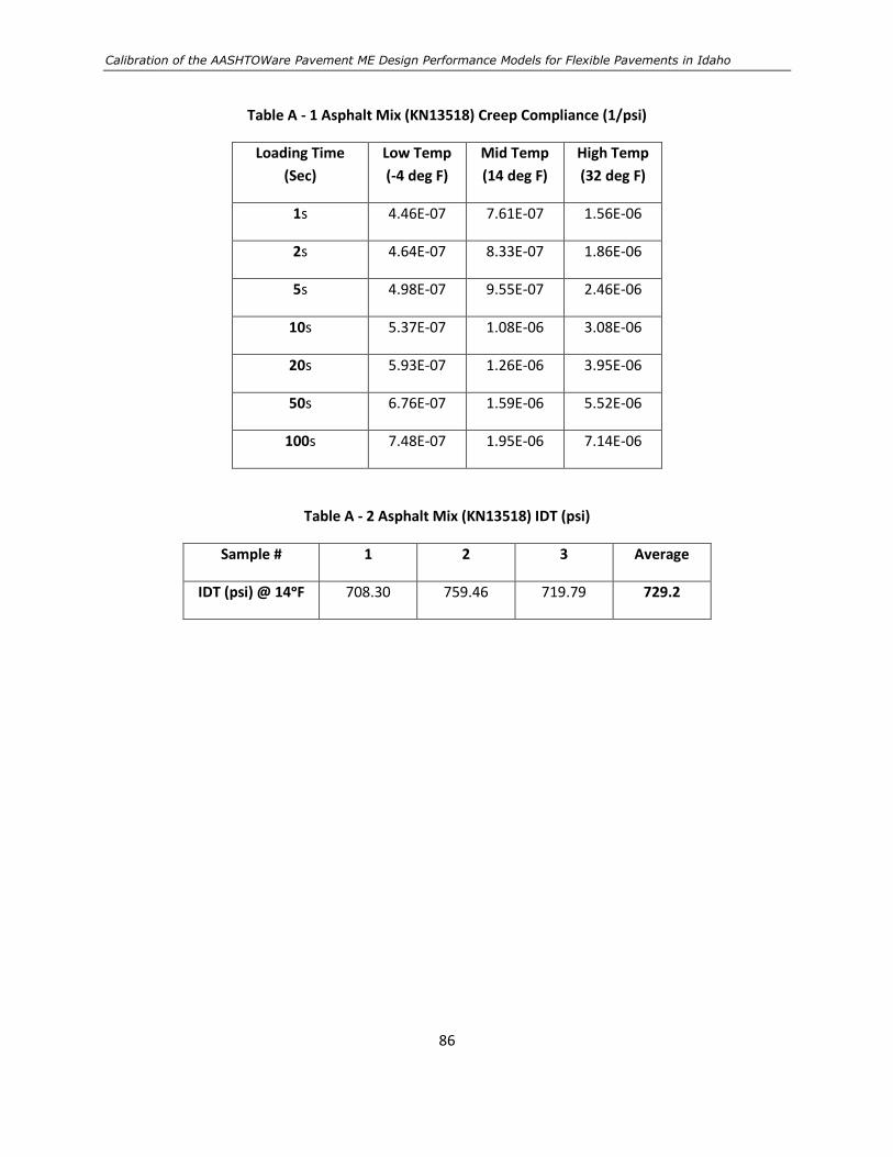
Calibration of the AASHTOWare Pavement ME Design Performance Models for Flexible Pavements in Idaho
86
Table A - 1 Asphalt Mix (KN13518) Creep Compliance (1/psi)
Loading Time
(Sec)
Low Temp
(-4 deg F)
Mid Temp
(14 deg F)
High Temp
(32 deg F)
1s 4.46E-07 7.61E-07 1.56E-06
2s 4.64E-07 8.33E-07 1.86E-06
5s 4.98E-07 9.55E-07 2.46E-06
10s 5.37E-07 1.08E-06 3.08E-06
20s 5.93E-07 1.26E-06 3.95E-06
50s 6.76E-07 1.59E-06 5.52E-06
100s 7.48E-07 1.95E-06 7.14E-06
Table A - 2 Asphalt Mix (KN13518) IDT (psi)
Sample # 1 2 3 Average
IDT (psi) @ 14ᵒF 708.30 759.46 719.79 729.2

Appendix A
87
Table A - 3 Asphalt Mix (KN9458) Creep Compliance (1/psi)
Loading Time
(Sec)
Low Temp
(-4 deg F)
Mid Temp
(14 deg F)
High Temp
(32 deg F)
1s 1.28E-08 1.16E-07 2.65E-07
2s 1.55E-08 2.52E-07 4.39E-07
5s 5.93E-08 5.29E-07 8.82E-07
10s 6.40E-08 9.31E-07 1.61E-06
20s 1.18E-07 1.49E-06 2.68E-06
50s 2.15E-07 2.76E-06 4.79E-06
100s 3.99E-07 4.43E-06 7.84E-06
Table A - 4 Asphalt Mix (KN9458) IDT (psi)
Sample # 1 2 3 Average
IDT (psi) @ 14ᵒF 484.27 405.99 379.58 423.3

Calibration of the AASHTOWare Pavement ME Design Performance Models for Flexible Pavements in Idaho
88
Table A - 5 Asphalt Mix (KN 11686) Creep Compliance (1/psi)
Loading Time
(Sec)
Low Temp
(-4 deg F)
Mid Temp
(14 deg F)
High Temp
(32 deg F)
1s 3.71E-07 6.93E-07 1.42E-06
2s 3.95E-07 7.88E-07 1.71E-06
5s 4.15E-07 9.41E-07 2.11E-06
10s 4.64E-07 1.11E-06 2.53E-06
20s 5.15E-07 1.32E-06 3.12E-06
50s 6.29E-07 1.61E-06 4.15E-06
100s 6.77E-07 1.85E-06 5.13E-06
Table A - 6 Asphalt Mix (KN 11686) IDT (psi)
Sample # 1 2 3 Average
IDT (psi) @ 14ᵒF 959.78 869.73 861.18 896.9

Appendix A
89
Table A - 7 Asphalt Mix (KN 13823) Creep Compliance (1/psi)
Loading Time
(Sec)
Low Temp
(-4 deg F)
Mid Temp
(14 deg F)
High Temp
(32 deg F)
1s 2.44E-07 3.90E-07 5.27E-07
2s 2.46E-07 4.03E-07 5.97E-07
5s 2.68E-07 4.57E-07 7.21E-07
10s 3.07E-07 4.90E-07 8.63E-07
20s 3.08E-07 5.35E-07 1.09E-06
50s 3.52E-07 6.15E-07 1.57E-06
100s 3.83E-07 7.16E-07 2.08E-06
Table A - 8 Asphalt Mix (KN 13823) IDT (psi)
Sample # 1 2 3 Average
IDT (psi) @ 14ᵒF 613.42 611.49 697.23 640.7

Calibration of the AASHTOWare Pavement ME Design Performance Models for Flexible Pavements in Idaho
90
Table A - 9 Asphalt Mix (KN 13552) Creep Compliance (1/psi)
Loading Time
(Sec)
Low Temp
(-4 deg F)
Mid Temp
(14 deg F)
High Temp
(32 deg F)
1s 1.70E-08 3.74E-09 2.49E-08
2s 8.42E-09 2.00E-08 6.31E-09
5s 5.88E-10 2.07E-08 1.24E-08
10s -1.28E-08 2.04E-09 5.57E-09
20s 8.38E-09 4.48E-09 2.14E-08
50s 4.39E-08 3.75E-08 1.41E-07
100s 6.54E-08 1.54E-07 4.41E-07
Table A - 10 Asphalt Mix (KN 13552) IDT (psi)
Sample # 1 2 3 Average
IDT (psi) @ 14ᵒF 511.68 560.24 458.71 510.2
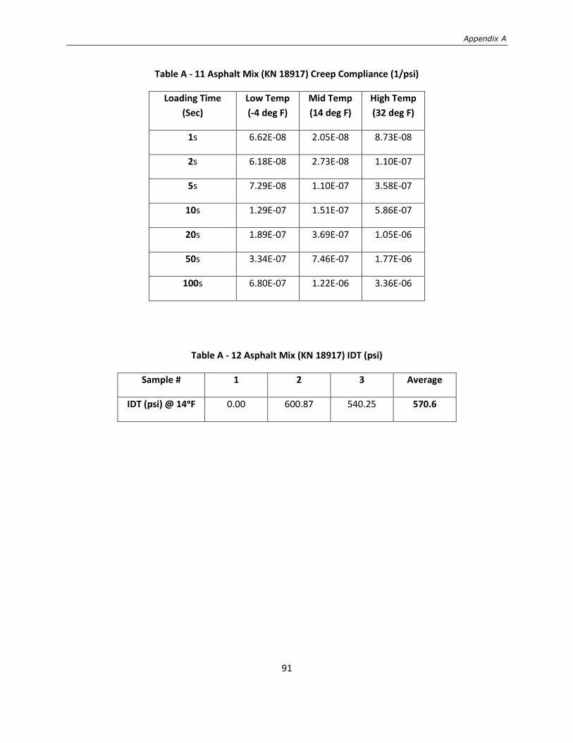
Appendix A
91
Table A - 11 Asphalt Mix (KN 18917) Creep Compliance (1/psi)
Loading Time
(Sec)
Low Temp
(-4 deg F)
Mid Temp
(14 deg F)
High Temp
(32 deg F)
1s 6.62E-08 2.05E-08 8.73E-08
2s 6.18E-08 2.73E-08 1.10E-07
5s 7.29E-08 1.10E-07 3.58E-07
10s 1.29E-07 1.51E-07 5.86E-07
20s 1.89E-07 3.69E-07 1.05E-06
50s 3.34E-07 7.46E-07 1.77E-06
100s 6.80E-07 1.22E-06 3.36E-06
Table A - 12 Asphalt Mix (KN 18917) IDT (psi)
Sample # 1 2 3 Average
IDT (psi) @ 14ᵒF 0.00 600.87 540.25 570.6

Calibration of the AASHTOWare Pavement ME Design Performance Models for Flexible Pavements in Idaho
92
Table A - 13 Asphalt Mix (KN 13923) Creep Compliance (1/psi)
Loading Time
(Sec)
Low Temp
(-4 deg F)
Mid Temp
(14 deg F)
High Temp
(32 deg F)
1s 4.53E-07 6.45E-07 1.39E-06
2s 4.84E-07 7.28E-07 1.63E-06
5s 5.13E-07 8.36E-07 2.10E-06
10s 5.78E-07 9.67E-07 2.64E-06
20s 6.11E-07 1.13E-06 3.36E-06
50s 6.75E-07 1.42E-06 4.79E-06
100s 7.74E-07 1.75E-06 6.25E-06
Table A - 14 Asphalt Mix (KN 13923) IDT (psi)
Sample # 1 2 3 Average
IDT (psi) @ 14ᵒF 790.44 754.90 719.25 754.9

Appendix A
93
Table A - 15 Asphalt Mix (KN 12046) Creep Compliance (1/psi)
Loading Time
(Sec)
Low Temp
(-4 deg F)
Mid Temp
(14 deg F)
High Temp
(32 deg F)
1s 3.54E-07 4.91E-07 7.12E-07
2s 3.56E-07 5.21E-07 8.03E-07
5s 3.84E-07 5.81E-07 1.10E-06
10s 4.04E-07 6.25E-07 1.39E-06
20s 4.27E-07 6.94E-07 1.78E-06
50s 4.65E-07 8.62E-07 2.51E-06
100s 4.85E-07 1.01E-06 3.30E-06
Table A - 16 Asphalt Mix (KN 12046) IDT (psi)
Sample # 1 2 3 Average
IDT (psi) @ 14ᵒF 573.80 511.63 621.72 569.1
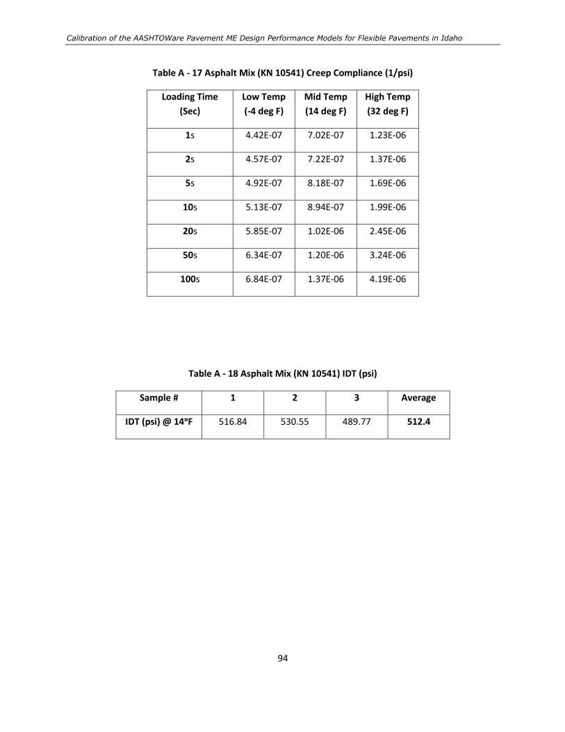
Calibration of the AASHTOWare Pavement ME Design Performance Models for Flexible Pavements in Idaho
94
Table A - 17 Asphalt Mix (KN 10541) Creep Compliance (1/psi)
Loading Time
(Sec)
Low Temp
(-4 deg F)
Mid Temp
(14 deg F)
High Temp
(32 deg F)
1s 4.42E-07 7.02E-07 1.23E-06
2s 4.57E-07 7.22E-07 1.37E-06
5s 4.92E-07 8.18E-07 1.69E-06
10s 5.13E-07 8.94E-07 1.99E-06
20s 5.85E-07 1.02E-06 2.45E-06
50s 6.34E-07 1.20E-06 3.24E-06
100s 6.84E-07 1.37E-06 4.19E-06
Table A - 18 Asphalt Mix (KN 10541) IDT (psi)
Sample # 1 2 3 Average
IDT (psi) @ 14ᵒF 516.84 530.55 489.77 512.4

Appendix A
95
Table A - 19 Asphalt Mix (KN 12212) Creep Compliance (1/psi)
Loading Time
(Sec)
Low Temp
(-4 deg F)
Mid Temp
(14 deg F)
High Temp
(32 deg F)
1s 2.35E-07 3.71E-07 6.38E-07
2s 2.56E-07 3.85E-07 6.94E-07
5s 2.52E-07 4.34E-07 9.03E-07
10s 2.68E-07 4.98E-07 1.09E-06
20s 2.79E-07 5.68E-07 1.37E-06
50s 2.91E-07 7.11E-07 2.16E-06
100s 3.26E-07 8.10E-07 2.95E-06
Table A - 20 Asphalt Mix (KN 12212) IDT (psi)
Sample # 1 2 3 Average
IDT (psi) @ 14ᵒF 720.34 667.50 688.28 692.0

Calibration of the AASHTOWare Pavement ME Design Performance Models for Flexible Pavements in Idaho
96
Table A - 21 Asphalt Mix (KN 12431) Creep Compliance (1/psi)
Loading Time
(Sec)
Low Temp
(-4 deg F)
Mid Temp
(14 deg F)
High Temp
(32 deg F)
1s 4.01E-07 6.79E-07 1.66E-06
2s 4.33E-07 7.31E-07 1.99E-06
5s 4.74E-07 8.89E-07 2.72E-06
10s 5.10E-07 1.06E-06 3.59E-06
20s 5.62E-07 1.33E-06 4.77E-06
50s 6.62E-07 1.72E-06 7.00E-06
100s 7.70E-07 2.10E-06 9.20E-06
Table A - 22 Asphalt Mix (KN 12431) IDT (psi)
Sample # 1 2 3 Average
IDT (psi) @ 14ᵒF 594.70 641.79 645.69 627.4

Appendix A
97
Table A - 23 Asphalt Mix (KN 13079) Creep Compliance (1/psi)
Loading Time
(Sec)
Low Temp
(-4 deg F)
Mid Temp
(14 deg F)
High Temp
(32 deg F)
1s 5.73E-09 8.69E-08 1.02E-07
2s 1.69E-08 1.65E-07 2.35E-07
5s 9.26E-08 4.00E-07 7.01E-07
10s 1.93E-07 6.88E-07 1.41E-06
20s 3.46E-07 1.00E-06 2.41E-06
50s 5.82E-07 1.81E-06 4.26E-06
100s 9.28E-07 3.01E-06 7.19E-06
Table A - 24 Asphalt Mix (KN 13079) IDT (psi)
Sample # 1 2 3 Average
IDT (psi) @ 14ᵒF 406.84 493.99 504.53 468.5
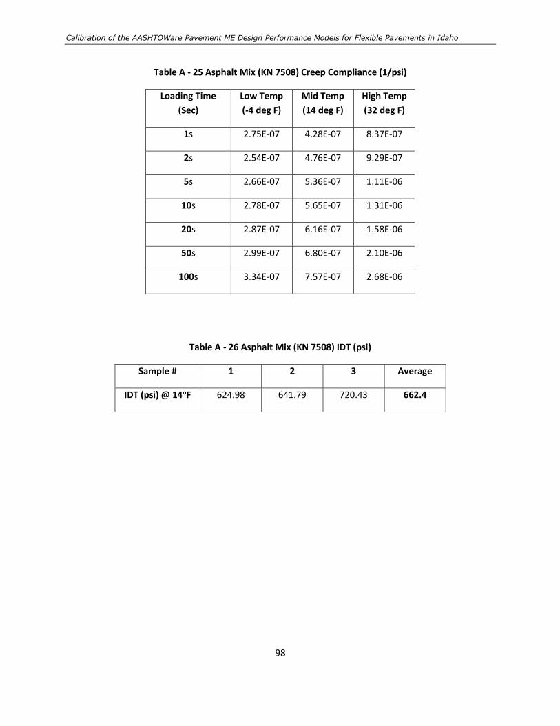
Calibration of the AASHTOWare Pavement ME Design Performance Models for Flexible Pavements in Idaho
98
Table A - 25 Asphalt Mix (KN 7508) Creep Compliance (1/psi)
Loading Time
(Sec)
Low Temp
(-4 deg F)
Mid Temp
(14 deg F)
High Temp
(32 deg F)
1s 2.75E-07 4.28E-07 8.37E-07
2s 2.54E-07 4.76E-07 9.29E-07
5s 2.66E-07 5.36E-07 1.11E-06
10s 2.78E-07 5.65E-07 1.31E-06
20s 2.87E-07 6.16E-07 1.58E-06
50s 2.99E-07 6.80E-07 2.10E-06
100s 3.34E-07 7.57E-07 2.68E-06
Table A - 26 Asphalt Mix (KN 7508) IDT (psi)
Sample # 1 2 3 Average
IDT (psi) @ 14ᵒF 624.98 641.79 720.43 662.4

Appendix A
99
Table A - 27 Asphalt Mix (KN 8454) Creep Compliance (1/psi)
Loading Time
(Sec)
Low Temp
(-4 deg F)
Mid Temp
(14 deg F)
High Temp
(32 deg F)
1s 2.27E-08 6.48E-08 9.88E-08
2s 3.28E-08 1.72E-07 1.71E-07
5s 1.15E-07 3.88E-07 4.53E-07
10s 2.26E-07 6.39E-07 8.39E-07
20s 5.59E-07 1.10E-06 1.26E-06
50s 9.91E-07 1.93E-06 2.42E-06
100s 1.63E-06 3.05E-06 3.62E-06
Table A - 28 Asphalt Mix (KN 8454) IDT (psi)
Sample # 1 2 3 Average
IDT (psi) @ 14ᵒF 544.40 411.36 380.03 445.3

Calibration of the AASHTOWare Pavement ME Design Performance Models for Flexible Pavements in Idaho
100
Table A - 29 Asphalt Mix (KN 13435) Creep Compliance (1/psi)
Loading Time
(Sec)
Low Temp
(-4 deg F)
Mid Temp
(14 deg F)
High Temp
(32 deg F)
1s 2.82E-07 1.53E-07 2.88E-07
2s 2.99E-07 1.64E-07 3.69E-07
5s 3.17E-07 1.85E-07 4.91E-07
10s 3.39E-07 2.09E-07 5.25E-07
20s 3.50E-07 2.35E-07 6.33E-07
50s 3.89E-07 2.84E-07 8.36E-07
100s 4.07E-07 3.35E-07 1.14E-06
Table A - 30 Asphalt Mix (KN 13435) IDT (psi)
Sample # 1 2 3 Average
IDT (psi) @ 14ᵒF 776.07 725.20 709.17 736.8

Appendix A
101
Table A - 31 Asphalt Mix (KN 10939) Creep Compliance (1/psi)
Loading Time
(Sec)
Low Temp
(-4 deg F)
Mid Temp
(14 deg F)
High Temp
(32 deg F)
1s 4.39E-07 6.93E-07 1.23E-06
2s 4.80E-07 7.48E-07 1.40E-06
5s 5.21E-07 8.37E-07 1.70E-06
10s 5.42E-07 9.30E-07 2.06E-06
20s 5.67E-07 1.07E-06 2.56E-06
50s 6.31E-07 1.29E-06 3.52E-06
100s 6.84E-07 1.56E-06 4.58E-06
Table A - 32 Asphalt Mix (KN 10939) IDT (psi)
Sample # 1 2 3 Average
IDT (psi) @ 14ᵒF 522.37 542.41 533.74 532.8
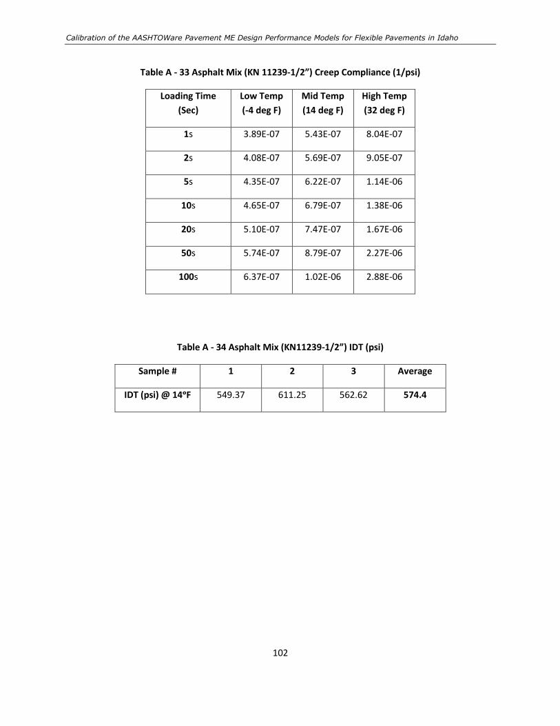
Calibration of the AASHTOWare Pavement ME Design Performance Models for Flexible Pavements in Idaho
102
Table A - 33 Asphalt Mix (KN 11239-1/2”) Creep Compliance (1/psi)
Loading Time
(Sec)
Low Temp
(-4 deg F)
Mid Temp
(14 deg F)
High Temp
(32 deg F)
1s 3.89E-07 5.43E-07 8.04E-07
2s 4.08E-07 5.69E-07 9.05E-07
5s 4.35E-07 6.22E-07 1.14E-06
10s 4.65E-07 6.79E-07 1.38E-06
20s 5.10E-07 7.47E-07 1.67E-06
50s 5.74E-07 8.79E-07 2.27E-06
100s 6.37E-07 1.02E-06 2.88E-06
Table A - 34 Asphalt Mix (KN11239-1/2”) IDT (psi)
Sample # 1 2 3 Average
IDT (psi) @ 14ᵒF 549.37 611.25 562.62 574.4
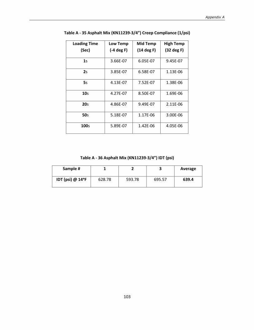
Appendix A
103
Table A - 35 Asphalt Mix (KN11239-3/4”) Creep Compliance (1/psi)
Loading Time
(Sec)
Low Temp
(-4 deg F)
Mid Temp
(14 deg F)
High Temp
(32 deg F)
1s 3.66E-07 6.05E-07 9.45E-07
2s 3.85E-07 6.58E-07 1.13E-06
5s 4.13E-07 7.52E-07 1.38E-06
10s 4.27E-07 8.50E-07 1.69E-06
20s 4.86E-07 9.49E-07 2.11E-06
50s 5.18E-07 1.17E-06 3.00E-06
100s 5.89E-07 1.42E-06 4.05E-06
Table A - 36 Asphalt Mix (KN11239-3/4”) IDT (psi)
Sample # 1 2 3 Average
IDT (psi) @ 14ᵒF 628.78 593.78 695.57 639.4

Calibration of the AASHTOWare Pavement ME Design Performance Models for Flexible Pavements in Idaho
104

Appendix B
105
Appendix B Performance Database
(e-file)

Calibration of the AASHTOWare Pavement ME Design Performance Models for Flexible Pavements in Idaho
106

Appendix B
107