University of Arkansas, FayettevilleScholarWorks@UARK

Theses and Dissertations

12-2014

Calibration of Resistance Factors for Driven Pilesusing Static and Dynamic TestsDeshinka A. BostwickUniversity of Arkansas, Fayetteville

Follow this and additional works at: http://scholarworks.uark.edu/etd

Part of the Geotechnical Engineering Commons

This Thesis is brought to you for free and open access by ScholarWorks@UARK. It has been accepted for inclusion in Theses and Dissertations by anauthorized administrator of ScholarWorks@UARK. For more information, please contact scholar@uark.edu, ccmiddle@uark.edu.

Recommended CitationBostwick, Deshinka A., "Calibration of Resistance Factors for Driven Piles using Static and Dynamic Tests" (2014). Theses andDissertations. 2059.http://scholarworks.uark.edu/etd/2059

Calibration of Resistance Factors for Driven Piles using Static and Dynamic Tests

Calibration of Resistance Factors for Driven Piles using Static and Dynamic Tests

A thesis submitted in partial fulfillment

of the requirements for the degree of

Master of Science in Civil Engineering

By

Deshinka Arimena Bostwick

University of Arkansas

Bachelor of Science in Civil Engineering, 2011

December 2014

University of Arkansas

This thesis is approved for recommendation to the Graduate Council.

Dr. Norman D. Dennis

Thesis Director

Dr. Richard A. Coffman

Committee Member

Dr. Rodney D. Williams

Committee Member

Abstract

The field of geotechnical engineering has evolved from Allowable Stress Design (ASD)

to Load Factor and Resistance Design (LRFD) which has led to a need to quantify the measures

of uncertainty and the level of reliability associated with a project. The measures of uncertainty

are quantified by load and resistance factors, while the level of reliability is driven by the amount

of risk an owner is willing to take and is quantified by the reliability index. The load factors are

defined through structural design codes, but the resistance factors have uncertainties that can be

mitigated through reliability based design. The American Association of State Highway and

Transportation Officials (AASHTO) have recommended resistance factors that are dependent on

the type of load tests conducted and are available as a reference to state agencies. The objective

of this study was to improve the AASHTO recommended resistance factors used by the Arkansas

State Highway and Transportation Department (AHTD), thereby, increasing allowable pile

capacity and reducing deep foundation costs. Revised resistance factors for field acceptance

based on dynamic testing were established through the analysis of pile load test data where both

static and dynamic load testing was conducted. Pile load tests were separated by pile type and

soil type. It was important that the load test data analyzed represented soil and geologic

conditions similar to those found in Arkansas. The resistance factors determined from this

analysis improved AHTD current practice, but indicated that the factors recommended by

AASHTO may be unconservative for this region.

© by Deshinka Arimena Bostwick

All Rights Reserved.

Acknowledgments

A note of appreciation is extended to my family for their support throughout this journey,

also to the professors and lecturers throughout my academic career.

Table of Contents

1 Introduction ............................................................................................................................. 1

1.1 Problem Statement ............................................................................................................ 2

1.2 Research Objectives .......................................................................................................... 4

2 Literature Review .................................................................................................................... 6

2.1 Introduction ....................................................................................................................... 6

2.1 Overview of Design and Testing of Pile Foundations ...................................................... 7

2.2 Static Design ...................................................................................................................... 8

2.3 Dynamic Formulae .......................................................................................................... 10

2.3.1 Engineering News (EN) Formula ...................................................................... 11

2.3.2 The Gates Formula ............................................................................................. 11

2.3.1 Modified Gates Formula .................................................................................... 12

2.3.2 Modified Engineering News (EN) Formula ...................................................... 12

2.3.3 The FHWA Gates Formula ................................................................................ 13

2.3.4 Washington State Department of Transportation (WSDOT) Formula .............. 14

2.4 Wave Equation Analysis ................................................................................................. 14

2.5 Static Load Testing .......................................................................................................... 17

2.5.1 Failure Criteria ................................................................................................... 20

2.6 Dynamic Load Tests ........................................................................................................ 26

2.6.1 Dynamic Load Testing with Signal Matching ................................................... 27

2.7 A Preferred Pile Load Evaluator (Newton’s APPLE) ..................................................... 30

2.8 Statnamic Load Testing ................................................................................................... 31

2.9 Case Study - A Comparison of SLT to DLT Capacity Values ....................................... 31

2.10 Geotechnical Design Process and Reliability .................................................................. 32

2.11 Reliability and LRFD Design .......................................................................................... 36

2.11.1 Statistical Terms................................................................................................. 38

2.11.2 First Order Second Moment (FOSM) ................................................................ 39

2.11.3 First Order Reliability Method (FORM)............................................................ 42

2.11.4 Monte Carlo Simulation ..................................................................................... 45

2.12 Summary ......................................................................................................................... 47

3 Methodology ......................................................................................................................... 48

3.1 Introduction ..................................................................................................................... 48

3.1 Database Development .................................................................................................... 49

3.1.1 Determining Soil Profile .................................................................................... 49

3.1.2 Louisiana Load Cases ........................................................................................ 51

3.1.3 Missouri Load Cases .......................................................................................... 52

3.1.4 Alabama Load Cases.......................................................................................... 52

3.2 Other Data from Literature .............................................................................................. 53

3.2.1 WSDOT ............................................................................................................. 53

3.2.2 PILOT - IOWA .................................................................................................. 54

3.2.3 FHWA - Central Artery/Tunnel (CA/T) Project, Boston, Massachusetts ......... 54

3.3 Data Analysis .................................................................................................................. 55

3.3.1 Regression Analysis ........................................................................................... 56

3.3.2 Robust Regression and Iterative Least Squares Fitting Techniques .................. 56

3.3.3 Probability Density Function (PDF) .................................................................. 58

3.3.4 Cumulative Probability Function (CDF) ........................................................... 59

3.3.5 Fisher Information Matrix and Confidence Interval .......................................... 60

3.3.6 Chi-Squared Goodness-Of-Fit Test ................................................................... 61

3.4 Calculation of Resistance (ϕ) Factors .............................................................................. 62

3.4.1 Parameters .......................................................................................................... 62

3.4.2 First Order Second Moment (FOSM) ................................................................ 64

3.4.3 First Order Reliability Method (FORM)............................................................ 65

3.4.4 Monte Carlo Simulation (MCS)......................................................................... 66

3.5 Summary ......................................................................................................................... 67

4 Results and Discussions ........................................................................................................ 69

4.1 General Analysis of All Piles .......................................................................................... 71

4.2 Case 2: Steel H-Piles in Clay Soil ................................................................................... 74

4.2.1 Linear Regression Analysis ............................................................................... 74

4.2.2 Probability Density Function (PDF) .................................................................. 76

4.2.3 Cumulative Distribution Function (CDF) .......................................................... 79

4.2.4 Chi-Squared Goodness-Of-Fit Test ................................................................... 83

4.2.5 Confidence Bounds at 95.0% Confidence Level ............................................... 84

4.3 Case 4: Steel H-Piles in Sand Soil ................................................................................... 86

4.4 Case 7 and Case 9: Precast Pre-stressed Concrete Piles (PPC/PSC) in Clay and Sand .. 89

4.5 Case 10: All Piles with Beginning of Restrike Capacities .............................................. 89

4.6 Calibration of Resistance (ϕ) Factors .............................................................................. 91

4.7 Analysis of Piles in Paikowsky 2004 Report .................................................................. 94

4.8 Efficiency ........................................................................................................................ 95

4.9 BOR Resistance Factors with Reliability Indexes .......................................................... 95

4.10 Summary ......................................................................................................................... 96

5 Conclusions ........................................................................................................................... 97

5.1 Future Work .................................................................................................................... 98

References. .................................................................................................................................. 100

Appendix A – Load Test Database ............................................................................................. 106

Appendix B – ReliaPile Graphs for Cases 7 and 9 ..................................................................... 113

List of Tables

Table 2.1. Effective stress and capacity development in driven piles (Long et al 1999) ............. 19 Table 2.2 Pile capacity with time for static analysis, SLT, and DLT performed

on the Caminada Bay Bridge Project. ............................................................................... 32 Table 2.3 Excerpt for resistance factors for driven piles (AASHTO 2010) ................................. 36 Table 3.1. Statistical characteristics of loads used for resistance

factor calibration (Paikowsky 2004) ................................................................................. 63 Table 3.2 Relationship between reliability index and probability of failure

(Paikowsky et al. 2010)..................................................................................................... 64 Table 4.1. Summary characteristics of the 138 load tests contained in the load test database. .... 70 Table 4.2. Pile load tests cases with quantity of piles ................................................................... 71 Table 4.3. Summary of statistical parameters for each group of pile load cases. ......................... 82

Table 4.4. Chi-Squared Test for Cumulative Distribution Function (CDF) for Case 1 through

Case 11 .............................................................................................................................. 84

Table 4.5. Resistance factors (ϕ) for target reliability index (βT) of 3.0 (non-redundant piles) and

2.33 (redundant piles) ....................................................................................................... 93

Table A.1. Load test database ..................................................................................................... 106

List of Figures

Figure 2.1. Pile-soil model for wave equation calculations (Smith 1962) .................................... 16 Figure 2.2. Schematic of static load testing (ASTM D1143/D1143M 2007) ............................... 18

Figure 2.3. SLT load-settlement curve illustrating loading to plunging failure and illustrating the

application of the Davisson-offset failure criterion (Reese et al. 2006) ........................... 20 Figure 2.4. Davisson Offset Limit example (Fellenius 2001) ...................................................... 24 Figure 2.5. DeBeer Yield Limit example (Fellenius 2001) .......................................................... 24 Figure 2.6. Hansen 80% criterion example (Fellenius 2001) ....................................................... 25

Figure 2.7. Chin-Kondner Extrapolation example (Fellenius 2001) ............................................ 25 Figure 2.8. Decourt Extrapolation example (Fellenius 2001) ....................................................... 26 Figure 2.9. Strain gauge and accelerometer attached to a pile for dynamic testing

(http://www.pile.com/aboutdynamictesting/) ................................................................... 27

Figure 2.10. Example of CAPWAP signal matching (FHWA-HRT-05-159 2006) ..................... 29 Figure 2.11. Newton’s APPLE loading system (http://www.dot.state.oh.us/) ............................. 30 Figure 2.12 An illustration of the probability density function for load factor and resistance

factors (Paikowsky 2002) ................................................................................................. 35 Figure 2.13 The performance function for a normal distribution (g(R,Q)) demonstrating the

margin of safety (pf) and its relation to the reliability index, β (σg = standard deviation of

g) (Paikowsky et al. 2010) ................................................................................................ 37

Figure 3.1. The geology of Arkansas (www.geology.ar.gov) ...................................................... 50 Figure 4.1. Scatter plot of all the load tests analyzed at EOD (Case 1) ........................................ 72 Figure 4.2. Scatter plot of all the load tests analyzed at BOR (Case 10) ...................................... 73

Figure 4.3. Microsoft Excel® linear regression plot for steel H-Piles in clay soil (Case 2) ........ 75 Figure 4.4. ReliaPile linear regression plot for steel H-Piles in clay soil (Case 2) ....................... 76

Figure 4.5. Microsoft Excel® probability density function plot (PDF) of steel H-Piles in clay soil

(Case 2) ............................................................................................................................. 78

Figure 4.6. ReliaPile probability density function plot (PDF) of steel H-Piles in clay soil (Case 2)

........................................................................................................................................... 79 Figure 4.7. Microsoft Excel® cumulative distribution function plot (CDF) of steel H-Piles in

clay soil (Case 2) ............................................................................................................... 81 Figure 4.8. ReliaPile cumulative distribution function plot (CDF) of steel H-Piles in clay soil

(Case 2) ............................................................................................................................. 81 Figure 4.9. Microsoft Excel® confidence bounds for Predicted Log-Normal Distribution at

95.0% Confidence Level of steel H-Piles in clay soil (Case 2) ........................................ 85

Figure 4.10. ReliaPile confidence bounds for Predicted Log-Normal Distribution at 95.0%

Confidence Level of steel H-Piles in clay soil (Case 2) ................................................... 85

Figure 4.11. ReliaPile linear regression plot for steel H-Piles in sandy soil (Case 4) .................. 87 Figure 4.12. ReliaPile probability density function plot (PDF) of steel H-Piles in sandy soil

(Case 4) ............................................................................................................................. 87 Figure 4.13. ReliaPile cumulative distribution function plot (CDF) of steel H-Piles in sandy soil

(Case 4) ............................................................................................................................. 88 Figure 4.14. ReliaPile confidence bounds for Predicted Log-Normal Distribution at 95.0%

Confidence Level of steel H-Piles in sandy soil (Case 4) ................................................. 88

Figure 4.15. ReliaPile probability density function plot (PDF) of all piles with BOR data

(Case 10) ........................................................................................................................... 90

Figure 4.16. ReliaPile cumulative distribution function plot (CDF) of all piles with BOR data

(Case 10) ........................................................................................................................... 90 Figure 4.17. ReliaPile confidence bounds for Predicted Log-Normal Distribution at 95%

Confidence Level of all piles with BOR data (Case 10). .................................................. 91

Figure B.1. ReliaPile Linear Regression Plot for PPC piles in clay soil (Case 7) ...................... 113 Figure B.2. ReliaPile Probability Density Function Plot (PDF) for PPC piles in clay soil

(Case 7) ........................................................................................................................... 114 Figure B.3. ReliaPile Cumulative Distribution Function Plot (CDF) for PPC piles in clay soil

(Case 7) ........................................................................................................................... 114

Figure B.4. ReliaPile Confidence Bounds for Predicted Log-Normal Distribution at 95.0%

Confidence Level for PPC piles in clay soil (Case 7) ..................................................... 115 Figure B.5. ReliaPile Linear Regression Plot for PPC piles in sand soil (Case 9) ..................... 115 Figure B.6. ReliaPile Probability Density Function Plot (PDF) for PPC piles in sand soil (Case 9)

......................................................................................................................................... 116 Figure B.7. ReliaPile Cumulative Distribution Function Plot (CDF) for PPC piles in sand soil

(Case 9) ........................................................................................................................... 116 Figure B.8. ReliaPile Confidence Bounds for Predicted Log-Normal Distribution at 95.0%

Confidence Level for PPC piles in sand soil (Case 9) .................................................... 117

1

1 Introduction

Pile foundations become a critical aspect in construction when the structural loads from

buildings and bridges must be transferred from relatively weak surface soils to stronger soil or

rock stratigraphy. Pile foundations offer additional load carrying capability that is essential for

foundations that must sustain large structural loads with relatively small settlements. The design

of pile foundations is subject to a large number of uncertainties which can lead to over

conservative or unconservative designs if care is not taken to address these uncertainties in a

logical and realistic manner. These uncertainties can be mitigated through the proper application

of factors of safety to design loads and full scale pile testing. Clearly, managing uncertainty is

necessary to ensure economic and efficient use of resources, time, and money.

When piles are installed, seldom are full scale load tests performed that provide definitive

values for capacity. When capacity is known precisely for test piles, production piles can be

redesigned or pile groups redistributed thereby reducing costs. Pile capacity is truly measured by

performing static load testing (SLT). Unfortunately, SLT is very expensive, the cost ranges from

$50,000 to $2 million depending on the intended size and capacity of the pile, the need for

sophisticated reaction pile systems, and mobilization costs (Loadtest USA 2012). As a distinct

result, industry practice is to use other less costly procedures to predict pile capacity.

Dynamic load testing (DLT) through signal matching and the use of program interface

software such as the pile driving analyzer (PDA) and CAse Pile Wave Analyses Program

(CAPWAP) have become an accepted means to predict pile capacity in conjunction with wave

equation analysis. However, dynamic load testing is normally performed on only a small

selection of test piles to determine the driving criteria for the project and the possible pile

2

capacity development within the site. It would be ideal to test every pile driven on a site and

have capacity quantified, but due to time and money constraints, very few production piles are

actually tested. Testing a larger population of piles specific to a region can positively impact

current pile driving practices, prompting more efficient designs and better classification of

uncertainties.

Arkansas reportedly monitors fewer than 5% of production piles with signal matching to

establish a final production pile driving criteria (Brown et al. 2011). Due to having very little

applicable load test data, Arkansas pile design and field acceptance is guided by the guidelines of

the American Association of State Highway and Transportation Official (AASHTO) Load Factor

and Resistance Design (LRFD) Bridge Design Specifications. This guide provides

recommendations based on worldwide data than may misrepresent pile driving conditions in

Arkansas.

1.1 Problem Statement

Pile capacity is definitively measured through static load testing (SLT). While its use is

limited, this is the methodology that most accurately measures the ultimate capacity of pile

foundations. Unfortunately, this test method is often cost prohibitive, and as such, has seldom

been carried out in the state of Arkansas.

The Arkansas Highway and Transportation Department (AHTD) has estimated that 99

percent of the projects conducted by the agency involve pile foundations (Brown et al. 418

2011). Piles are driven to a specified driving resistance, characterized by blow count, which is

based on bearing capacity. Evidently, AHTD determines bearing capacity utilizing three distinct

methodologies: Empirical Pile Driving Formula (Method A), Wave Equation Analysis of Piles

3

(WEAP) (Method B), and Dynamic Load Testing (Method C) (Arkansas Specifications 2014).

The empirical formulas used in Method A calculate bearing capacity based solely on the weight

and stroke of the hammer used in driving (driving energy), and the penetration of the pile into the

soil per hammer blow. The safe bearing value for Method A is obtained when the target value is

maintained through the last five feet of driving or when practical refusal is observed. Practical

refusal occurs when the calculated safe bearing value is three times the required safe bearing

value. The current practice within AHTD is to implement a resistance factor of 0.1, which

corresponds to a dated Engineering News Record dynamic formula which does not consider the

pile-soil-hammer system.

Bearing capacity obtained through Method B, Wave Equation Analysis of Piles (WEAP),

matches the pile hammer to the pile and soil conditions. This method requires soil, pile, and

driving equipment properties, determined by the Engineer, to be entered into the Wave Equation

Analysis Program (WEAP). The analysis provides the Engineer with a bearing graph that shows

a hammer-blow count relationship for the required ultimate bearing capacity. The design bearing

capacity would be 40 % of the ultimate bearing capacity determined through WEAP, with a ϕ

factor of 0.40 (AASHTO 2010).

The bearing capacity obtained from Method C, Dynamic Load Testing, uses signal

matching to establish soil resistance to determine pile capacity. Bearing graphs are produced that

shows a hammer blow count relationship for 90% to 100% of the required ultimate bearing

capacity. The design bearing capacity of a pile shall be 40% of the ultimate bearing capacity as

determined by dynamic testing (AHTD 2007). In normal practice, however, piles are usually

driven to practical refusal or to rock. Currently, test piles on AHTD construction projects

4

constitute far less than 5% of production piles that are monitored by high strain dynamic testing

with signal matching (Brown et al. 2011).

Performing load testing on test piles provides the engineer with confirmation of design

capacity that is usually inferred through the analysis of boring log data and the use of empirical

design methods that may have unclear or unstated assumptions. The information obtained

through load testing, such as the pile ultimate bearing capacity and the load-settlement

relationship of the pile-soil system, can lead to a more informed decision on the allowable load

per pile, which may reduce the number and length of piles required for a given project, thereby

providing cost savings. The potential in cost savings may be sufficiently beneficial to encourage

the State of Arkansas to perform load testing on an increased number of test piles and to extend

testing to production piles. The expansion of pile testing should positively impact the

development of a pile load test database. A robust pile load database will allow for the

improvement of resistance factors used for the design and acceptance of pile foundations in the

State of Arkansas.

1.2 Research Objectives

The focus of this research effort will be to explore the correlation between SLT and DLT

methods. The endeavor is not to dissuade the use of SLT to measure pile capacity, but rather to

build a platform from which the AHTD can infer capacity predictions while implementing

appropriate resistance factors that are specific to the soil and pile type in question.

Accordingly, static and dynamic load test data from neighboring states with similar land

forms as Arkansas (Alabama, Missouri, Iowa, and Louisiana), will be collected, compiled and

analyzed. The information gathered is expected to allow AHTD to categorize projects by soil and

5

pile type, then choose the appropriate resistance factor for the project. The load test data would

encompass as many landforms as possible to allow observations on how different pile types

perform in a given stratigraphy.

The data reduction will be conducted by the University of Arkansas research team. The

main objectives of this research are: (1) Compare SLT capacities to DLT capacities; (2) Perform

statistical analysis of the load test data; (3) Develop resistance factors applicable to Arkansas; (4)

Determine the level of reliability of these design factors; (5) Refine a driven pile database for

Arkansas; (6) Provide guidance on field acceptance during pile driving.

To evaluate these objectives, several statistical methods will be performed at various levels

of reliability. Methods used to analyze the data will include a regression analysis, resistance

factor calibration through First Order Second Moment (FOSM), First Order Reliability Methods

(FORM), and the Monte Carlo Simulation (MCS) to determine a suitable resistance factors (ϕ)

appropriate for use in AHTD designs.

6

2 Literature Review

2.1 Introduction

Pile foundations have been the center of construction and the advancement of civilization

for thousands of years. The first records of pile use extend to the late Neolithic Period, about

9500 BC, with dwellings built in flood-prone areas. These early piles were formed by using

small trees which were denuded of branches. These timbers were then installed into the soil with

the small diameter at the bottom by a stone driving mechanism. These ancient pilings were also

used as the sub-structure of wooden bridges erected during the reign of Julius Caesar, 55 BC

(Ulitskii 1995).

Scientific studies involving the driving of piles were conducted as early as the 18th

century (Ulitskii 1995). These studies resulted in the use of dynamic capacity prediction

equations, the earliest of which were introduced by Woltmann and Eytelwein during the 19th

century (Ulitskii 1995; Chrimes 2008). These early dynamic equations considered the energy of

the pile driving hammer and the resulting pile set to determine bearing capacity (GRL Engineers,

Inc. 2014). Predicting pile capacity through dynamic formulae is variable and relies on the

expertise of the Engineer. Dynamic formulas can provide a wide range of capacity predictions,

depending on the input variables (soil properties, hammer efficiency, stroke of the ram, ram

weight, etc.) and thus may lead to over or under predicted capacities and expensive or unreliable

pile foundations.

To accurately measure pile capacity, an axial load is applied at the pile top and direct

measurements of displacement of the pile head are recorded. This type of capacity measurement

is termed Static Load Testing (SLT). The SLT is the most fundamental form of pile load testing

and is considered to be the bench-mark for pile load testing due to its repeatability and consistent

7

performance. Static Load Testing has been used to measure pile capacities ranging from 22 kips

to 2700 kips. Static Load Testing for piles with high capacities requires expensive pile reaction

systems. Pile capacity has also been determined through a less costly and more commonly

employed method called dynamic load testing (DLT). Dynamic load testing is a predictive

method, and is only as good as the inputs provided by the designer. Other methods to measure

pile capacity are the Statnamic Load Test and A Preferred Pile Load Evaluator (Newton’s

APPLE). Information necessary to accurately predict the pile capacity through dynamic methods

are the soil’s resistance, quake (displacement required to develop full soil capacity) and damping

coefficients. Both SLT and DLT are standardized by the American Society for Testing and

Materials (ASTM) and the American Association of State Highway and Traffic Officials.

(AASHTO) and provide the user with several testing methods which provide a varying array of

capacity measurement options.

2.1 Overview of Design and Testing of Pile Foundations

Determining the geometric and material properties of a pile for a deep foundation project

begins with the static design process. The following is a typical course the design process may

take: (1) The engineer is provided with the design loads and functions of the structure (critical or

non-critical), (2) sub surface soils investigations in which the engineer determines the number,

location and depth of borings needed to model the subsurface stratigraphy where the pile

foundation is to be constructed. The engineer must also specify sampling and testing protocols,

(3) Soil properties are evaluated through the interpretation of boring logs or cone penetration

data and laboratory testing (4) Empirical static analysis methods are conducted to determine the

pile size and length, and the number of piles necessary to safely resist the design load, (5)

Dynamic formulas are sometimes used to determine ultimate capacity of a pile based upon blow

8

counts of a particular hammer delivering a certain energy level. (6) Alternatively a stress wave

analysis could be conducted which integrates hammer, pile and soil properties to predict a pile

capacity as a function of blow count. (7) After all the initial calculations are made; field testing

should be conducted to measure pile capacity. The test pile may be instrumented and driven

while DLT is preformed or the pile may be subjected to SLT at some time after the pile driving.

Many agencies use a form of DLT called signal matching which has been shown to provide a

reliable correlation to SLT capacities. However, this DLT method is subject to some

uncertainties that may affect the predicted pile capacity. It is recommended that DLT and/or SLT

be performed after a 7 to 14 day waiting period to allow the soil time to either setup or relax after

the significant disturbance created by the driving operation. This would be the point in time

when the pile is most likely to exhibit its long-term capacity. When time and economics permit

SLT should be performed as this procedure is still the most reliable and truest measure of

capacity.

2.2 Static Design

Static analysis is an initial step in the pile foundation design and construction process that

establishes the geometry of the pile or pile group to develop a required resistance in a specified

soil profile. The essential soil parameters needed for design normally include: particle size,

plasticity, specific weight, strength, and location of the ground water table. These properties are

obtained through sub-surface exploration with the standard penetration test (SPT), cone

penetration tests (CPT), or undisturbed sampling of the soil. Interpretation of the information

obtained from sub-surface exploration will determine the method of analysis. Many

transportation agencies use the design methods contained in the computer program, DRIVEN 1.0

(FHWA 1998). This analysis program uses the Norlund β-method for sands or the Tomlinson α-

9

method for clays. Ultimate pile capacity (Qult) is determined through the summation of side

capacity (Qs) and tip capacity (Qp) for either method expressed in Eqn. 2.1, Eqn. 2.2, and Eqn.

2.3:

𝑄𝑢𝑙𝑡 = 𝑄𝑠 + 𝑄𝑝 Eqn. 2.1

𝑄𝑠 = 𝑓𝑠𝐴𝑠 Eqn. 2.2

Where: fs is the unit side resistance, As is the area of the pile side in contact with the soil.

𝑄𝑝 = 𝑞𝑝𝐴𝑝 Eqn. 2.3

Where: qp is the unit tip resistance, Ap is the area of the pile tip. For Norlund’s method the unit

side capacity, and the unit tip resistance are given by Eqn. 2.4:

𝑓𝑠 = 𝛽𝜎′𝑎𝑣𝑔, 𝛽 = 𝐾𝑡𝑎𝑛𝛿 and 𝑞𝑝 = 𝜎′𝑣𝑁𝑞 Eqn. 2.4

Where σ’avg is the average effective stress along the pile side, K is the earth pressure coefficient,

δ is the coefficient of wall friction, σ’v is the effective stress at the pile tip, and Nq is the

overburden bearing capacity factor. For the Tomlinson method the unit side and tip resistance

are given by Eqn. 2.5:

𝑓𝑠 = 𝛼𝐶𝑢 and 𝑞𝑝 = 9𝐶𝑢 Eqn. 2.5

Where: α is the adhesion factor, Cu is the undrained shear stress.

The Norlund β-method (Eqn. 2.4) for cohesionless soils and piles of uniform dimensions

was presented in 1963 by R. L. Norlund. It uses standard penetration blow count data to arrive at

a value of beta to be used in the equations described above (Norlund 1963). The Tomlinson α-

method (Eqn. 2.5) for cohesive soils was presented by M. J. Tomlinson (1957) and addresses the

change in the in-situ conditions of the soil as it is remolded while the pile is driven. Tomlinson

10

suggested a range of alpha values less than or equal to one that effectively reduce the soil’s

undrained shear strength. Other static design methods in common use include Meyerhof’s

method (Meyerhof 1976) for sands (Meyerhof 1976), American Petroleum Institute (API) (API

1984) for both sands and clays, and the Lambda I (Vijayvergiya et al. 1972) and Lambda II

(Kraft et al. 1981) methods for clays.

2.3 Dynamic Formulae

Once the pile geometry is established through static design methods, dynamic driving

formulas may be used to predict capacity as a function of pile penetration per hammer blow.

Dynamic formulae have been a common tool to predict pile capacity since the early 1900s

(Likins et al. 2012). The dynamic formula presented in Eqn. 2.6 is a potential energy balance

equation that relates the work energy transferred from the pile hammer to the pile as it penetrates

through a specific distance in the soil (Long et al. 2009). Dynamic formulae are generally

expressed as:

𝑒𝑊𝐻 = 𝑅𝑠 Eqn. 2.6

Where: e is the efficiency of the hammer, W is the weight of ram, H is the vertical drop of

hammer or stroke of ram, R is the pile resistance, and s is the pile permanent set. There have

been varied approaches to the development of dynamic formula throughout the years. The more

common methods include: the Engineering News (EN) formula; the Modified Engineering News

(EN) formula; the Gates formula; the Federal Highway Administration (FHWA) Gates formula;

and the Washington State Department of Transportation (WSDOT) formula.

11

2.3.1 Engineering News (EN) Formula

The Engineering News (EN) formula, illustrated in Eqn. 2.7, was developed in 1888 by

Arthur Mellen Wellington a railway civil engineer (Likins et al. 2012). This formula was

empirically developed for timber piles driven in sand with a drop hammer (Hannigan et al.

1998). Owing to the units used in the equation, it has a built-in factor of safety of six to produce

a safe load that a pile can support.

𝐿 = 𝐹 𝑊𝐻

(𝑠 + 𝑐)

Eqn. 2.7

Where: L is the safe load, F is a constant determined from experience, W is the ram weight, H is

the drop height of ram in feet (assumes single acting hammer), s is the penetration of pile in

inches per blow, and c is a constant to account for the elastic compression of the hammer-pile-

soil system. Historically, the EN formula has been considered the least accurate dynamic

predictive method. However, it is widely used among transportation departments due to its

simple formulation and ease of use. The EN formula has been proven to have factor of safeties

ranging from as low 0.5 to as high as 20 (FHWA 1998), yet 45% of respondents to the state of

practice survey reported in NCHRP Report 507 claim that they use the EN formula (Paikowsky

2004).

2.3.2 The Gates Formula

The Gates formula was proposed in 1957 by Marvin Gates, and is given in Eqn. 2.8. It is

an empirical equation that was developed by simplifying the form of existing equations and

adding an adjustment factor to achieve the allowable bearing capacity with a recommended

factor of safety of three.

12

𝑄𝑢 = (6

7) √𝑒𝐸𝑟 log(10𝑁𝑏)

Eqn. 2.8

Where: Qu is the ultimate pile capacity (kips), e is the efficiency of the hammer (taken as 75% for

drop hammers and 85% for all others), Er is the theoretical delivered energy of the pile hammer

(ft-lb), and Nb is the number of blows to cause one inch of pile penetration. The Gates formula

tends to over-predict resistance at low driving resistances and under-predict resistance at high

driving resistances (Allen 2005).

2.3.1 Modified Gates Formula

The analysis of 100 pile load tests (Olson et al. 1967) allowed for an adjustment in the

Gates formula to provide a better statistical fit through the measured and predicted data. The

formula was modified for timber with Eqn. 2.9, concrete with Eqn. 2.10, steel with Eqn. 2.11,

and all piles with Eqn. 2.12.

𝑅𝑢 = 1.11√𝑒𝐸𝑟 log(10𝑁𝑏) − 34 Eqn. 2.9

𝑅𝑢 = 1.39√𝑒𝐸𝑟 log(10𝑁𝑏) − 54 Eqn. 2.10

𝑅𝑢 = 2.01√𝑒𝐸𝑟 log(10𝑁𝑏) − 166 Eqn. 2.11

𝑅𝑢 = 1.55√𝑒𝐸𝑟 log(10𝑁𝑏) − 96 Eqn. 2.12

Where: Ru is the ultimate pile capacity (kips), e is the efficiency of the hammer (75% for drop

hammers or 85% for all others), Er is the theoretical delivered energy of the pile hammer (ft-lb),

and Nb is the number of blows to cause one inch of pile penetration.

2.3.2 Modified Engineering News (EN) Formula

The Modified Engineering News (EN) formula modifies the original EN formula by

accounting for the weight of the pile and the energy that may be lost in the transfer from hammer

13

to pile. Several modified EN formulas have been developed, but in 1965, the Michigan State

Highway Commission proposed an equation, expressed as Eqn. 2.13, that included a factor of

safety of 6.0 (Fragaszy et al. 1985).

𝑅𝑢 =𝑒ℎ 𝐸ℎ

(𝑠 + 𝑐)

𝑊 + 𝑛2𝑤

𝑊 + 𝑤

Eqn. 2.13

Where: Ru is the ultimate bearing capacity of pile in soil, eh is the efficiency of the striking

hammer (<1.0), Eh is the manufacturer’s hammer energy rating, s is the pile penetration for the

last blow count (set) in inches, c is a constant (0.1 for steam hammers or 1.0 for drop hammers),

W is the weight of the hammer ram, w is the weight of the pile, and n is the coefficient of

restitution of the pile material.

2.3.3 The FHWA Gates Formula

The FHWA Gates formula, presented in Eqn. 2.14, is the preferred dynamic formula to

predict bearing capacity (AASHTO 2010). Equation 2.8 is the original Gates formula modified

by Olson and Flaate in 1967 with the objective to have a better statistical fit through the

predicted and measured data (Long et al. 2009). The FHWA subsequently introduced more

modifications to the already modified Gates formula, producing the FHWA Gates formula which

takes the average of the equations for steel and concrete piles used in of the Modified Gates

equation. The FHWA Gates formula reduced the tendency to under predict capacity and has

demonstrated improved accuracy relative to the EN formula (Paikowsky et al. 2004; Allen

2005).

𝑅𝑛 = 1.75√𝐸𝑑 log(10𝑁𝑏) − 100 Eqn. 2.14

Where: Rn is the ultimate bearing resistance (kips), Ed is the developed hammer energy, and Nb is

the number of blows for one inch of pile penetration.

14

2.3.4 Washington State Department of Transportation (WSDOT) Formula

The WSDOT also attempted to improve upon the Gates (1957) formula which resulted in

significant changes as illustrated in Eqn. 2.15. The WSDOT formula was developed to maintain

the low prediction variability of the Gates Formula while simultaneously minimizing the

tendency to under- or over-predict resistance.

𝑅𝑛 = 6.6𝐹𝑒𝑓𝑓𝐸 Ln(10𝑁) Eqn. 2.15

Where: Rn is the ultimate bearing resistance (kips), Feff is the hammer efficiency factor, E is the

developed energy (ft-kips), Ln is the natural logarithm, in base “e”, and N is the average

penetration resistance in blows per inch for the last 4 inches of driving (WSDOT 2010).

Dynamic formulas are only one means of supplying an estimate of the pile capacity, it

addresses the kinetic energy of driving but not the entire driving system. It does not account for

pile cap, pile cushion, and other energy damping factors in the hammer-pile-soil system. It also

assumes constant soil resistance along the pile side (Long et al. 2009). In fact no soil parameters

are input into the equations, and they ignore the viscoelastic effects of the soil. Dynamic

formulae neglect pile axial stiffness effects while driving and assume the pile to be rigid

(Hannigan et al. 1998).

2.4 Wave Equation Analysis

The wave equation is a dynamic predictive method that represents a better relationship

between capacity and driving resistance. It relates pile penetration to stresses within the pile and

soil that presents a more complete picture of the hammer-pile-soil system and prevents the pile

from being loaded beyond the pile material capacity. The wave equation was first introduced by

Pochhaammer in 1876 as the analysis of a stress wave propagating through an infinitely long

15

cylindrical bar with a circular cross-section (Valsamos et al. 2013). As originally proposed, it

provides an equation of motion in an elastic medium and predicts no energy transfer (Kolsky

1963). After Pochhaammer, there were contributions made by Chree (1889) with an independent

theory on wave equations, Lord Rayleigh (1894) discussed it in sound theory, and Field (1931)

considered longitudinal waves (Kolsky 1963). In 1931 D.V. Isaacs had the idea of applying the

wave equation to pile driving.

However, it was not until 1960 that E.A.L. Smith proposed an approach that utilized a

numerical closed form solution to investigate the effects of the ram weight, ram velocity,

cushion, pile properties, and the soil’s dynamic behavior during driving. During Smith’s

investigation, the pile-soil model was fashioned into discretized lumped masses connected with

springs as illustrated in Figure 2.1. The governing equation for one-dimensional wave

propagation in a rod is a linear second order differential equation illustrated in Eqn. 2.16:

𝜎 = 𝜌𝜕2𝑢

𝜕𝑡2− 𝐸

𝜕2𝑢

𝜕𝑡2 Eqn. 2.16

Where: σ is the stress in the pile, ρ is the mass density of the pile, u is the axial displacement of a

point at location x on the pile at time t, ∂2u/∂t2 is acceleration of point x, and ∂2u/∂x2 is the strain

gradient at x at time t. Performing a wave equation analysis allows for the establishment of a

driving criterion and selection of the correct driving equipment for pile installation. The

drivability analysis of the system is predicated on the predicted static pile capacity with depth.

The wave equation provides a relationship between two sets of variables. The first set of

variables comprise: force, stress, and strain (Goble 2008). While the second set of variables

encompasses: displacement, velocity, and acceleration (Goble 2008). These variables help to

determine the stresses within the pile during driving. This method is semi-theoretical because it

16

depends on the accuracy of the soil, pile and hammer parameters entered into the equations. The

results of the wave equation provide rational and reliable pile capacities when compared to

values obtained from field tests (Reese et al. 2006). Wave equation analyses are performed on a

number of assumed pile capacities to construct a bearing graph that relates ultimate capacity to

driving resistance (Hannigan et al. 1998). The wave equation is used normally in conjunction

with SLT and DLT on pile foundations and appears to be a reliable predictor of the friction and

end bearing capacities of the pile.

Figure 2.1. Pile-soil model for wave equation calculations (Smith 1962)

17

2.5 Static Load Testing

The Static Load Test (SLT) is considered the most reliable testing method in the

verification of pile capacity in axial loading (Hannigan et al. 1997). Specifications for the

standard test method are stated in ASTM D1143/D1143M, ‘Standard Test Method for Piles

Under Static Axial Compressive Load’. This test specification defines seven SLT test

procedures, which are defined as follows: Quick Test (Procedure A), Maintained Load Test

(Procedure B), Loading in Excess of Maintained Test (Procedure C), Constant Time Interval

Test (Procedure D), Constant Rate of Penetration Test (Procedure E), Constant Movement

Increment Test (Procedure F), and the Cyclic Loading Test (Procedure G).

In all of the listed procedures the pile is loaded axially to failure or to a specified safe

structural capacity with the use of hydraulic jacks acting against the pile head and a reaction

frame as illustrated in Figure 2.2. Displacement gages or transducers and load cells are used to

acquire sufficient data to produce a load-settlement curve, which can be used to interpret

ultimate pile capacity. During research efforts, instrumented test piles make use of gages and

transducers attached to or embedded within the pile to record deformation measurements that can

be used to interpret the magnitude and the distribution of the static soil resistance along the pile

side and at the pile tip (Walton et al. 1998). Static load tests should be performed on driven piles

that have had equilibrium reestablished to the surrounding soil. Normally, a rest period from 3 to

30 days between driving and testing is needed to allow for any setup or relaxation in the

surrounding soil.

18

Figure 2.2. Schematic of static load testing (ASTM D1143/D1143M 2007)

Pile setup refers to the increase in effective stress with time as excess pore pressure,

generated during pile driving, is dissipated, which leads to increased pile capacity. When a pile is

driven into to clay, silt, or fine sand, excess positive pore pressure is developed as the water is

not able to translocate freely, given the nature of cohesive type soils. The soil and water is

displaced, causing the buildup of positive pore pressure, which results in lower effective stresses

around the pile (Hannigan 2009). As time passes, excess pore pressure dissipates and the soil

resistance around the pile increases, thereby increasing pile capacity. Relaxation on the other

hand is the reduction in effective stress with time; which reduces pile capacity. Driving a pile

into saturated dense silts or shales gives rise to negative pore pressures. As the soil and water are

displaced by the pile, the dense material dilates. This expansion under undrained conditions

19

essentially creates a vacuum in the void spaces, causing negative pore pressure (Hannigan 2009).

The phenomenon of set up and relaxation is summarized in Table 2.1.

Table 2.1. Effective stress and capacity development in driven piles (Long et al 1999)

Phenomena Effective Stress

Equation

End of Driving

(EOD)

After Pore

Pressures Dissipate

Setup 𝜎 = 𝜎 − (+𝑢) = 𝜎 − 𝑢 Low Effective Stress,

Low Capacity

Higher Effective Stress,

Higher Capacity

Relaxation 𝜎 = 𝜎 − (−𝑢) = 𝜎 + 𝑢

High Effective

Stress, High

Capacity

Lower Effective Stress,

Lower Capacity

Note: 𝜎 is effective stress, σ is total stress, and u is pore water pressure.

The Quick Test (Procedure A), is the most common method utilized by transportation

agencies due to its ease of use and satisfactory results (AASHTO 2010). The test pile is loaded

in increments of five percent (5%) of the anticipated failure load capacity. The load is maintained

for a fixed period of time that varies from four to fifteen (4-15) minutes. After achieving pile

failure, load is removed in approximately ten (10) equal decrements, the duration of the

unloading stages mirrors the duration for the loading stages (ASTM D1143/D1143M 2007). The

report provided from this test is an interpreted load-settlement curve which is illustrated in

Figure 2.3. Static load testing can range from $50,000 to $2 million depending on the reaction

pile setup (PDI 2013). A pile testing project for Milwaukee Stadium documents that SLT cost

$100,000 per test (PDI 2002).

20

Figure 2.3. SLT load-settlement curve illustrating loading to plunging failure and illustrating the

application of the Davisson-offset failure criterion (Reese et al. 2006)

2.5.1 Failure Criteria

The data generated from the static load test allows the ultimate capacity of a pile to be

identified according to a predefined failure criterion. According to a Manual presented in 1940

titled ‘Pile-Driving Formulas’, failure was defined as “the load that produced an increase in pile

movement disproportional to the increase in load” (Likins et al. 2012). In 1942 after review of

the Manual Report B, and through ASCE Journal Discussions, Karl Terzaghi sought the need to

add provisions to define the term “load at failure” (Terzaghi et al. 1942). Load at failure was then

defined as the load required to have the pile head move at least 10% of the pile tip diameter. This

standard was applicable to pile diameters of 12 inches, which was the typical pile diameter

installed during the period.

21

Since 1942, several researchers have developed improved techniques for determining

ultimate pile capacity through defining various failure criterion. It was necessary to develop

these techniques due to some load-test curves not having a well-defined failure load, and some

piles may never achieve ultimate capacity because of large toe capacities (Goble et al. 2000).

Ultimate pile capacity has been defined by: the Davisson Offset Limit, the DeBeer Yield Limit,

the Hansen 80% criterion, the Chin-Kondner Extrapolation, and the Decourt Extrapolation.

The most widely accepted method for defining ultimate pile capacity in North America is

the Davisson Offset Limit method proposed in 1972 (Davisson 1972). This technique, presented

in Eqn.2.17, produces a straight line parallel to and offset from a plot of the elastic compression

of the pile under load. This parallel line is superimposed on the load settlement curve illustrated

in Figure 2.3, at an offset of 0.15 inches plus the pile diameter (in inches) divided by 120. The

ultimate pile capacity is defined as the intersection of the Davisson offset and the load-settlement

curve, as illustrated in Figure 2.3. Pile head movement for piles with diameter less than 24 inches

is determined from Eqn.2.17 and Eqn.2.18 for piles with diameter larger than 24 inches. The

later equation, Eqn.2.18, is referred to as the modified Davisson Offset criterion recommended

by Kyfor et al. (1992):

𝛿𝑢 = 𝑄𝐿

𝐴𝐸+

𝐵

120+ 0.15(𝑖𝑛. )

Eqn.2.17

𝛿𝑢 = 𝑄𝐿

𝐴𝐸+

𝐵

30

Eqn.2.18

Where: δu is pile head movement, Q is the applied load, L is the pile length, A is the pile cross-

section area, E is the pile Modulus of Elasticity, and B is the pile diameter.

22

Another criterion used to identify the pile failure load is the DeBeer Yield Load,

introduced in 1968 (DeBeer 1968). It is an extrapolation method that is used when the data from

a load-settlement curve does not indicate a clear failure load. The load and settlement are plotted

using logarithmic scales, illustrated in Figure 2.5. At the development of the ultimate load, the

early linear portion of the load settlement curve begins to change slope, the point of the slope

change is classified as the yield load.

Another available extrapolation method is the Hansen 80% criterion introduced in 1963

(Hansen 1963). It uses the load-settlement curve to identify the point at which the applied load

produces four times the settlement that was observed for 80% of the same applied load. The

settlement is plotted against the square root of settlement divided by the load, illustrated in

Figure 2.6. The 80% criterion usually agrees with the plunging failure of the pile, and is usually

identified visually or can be computed by Eqn.2.19:

𝑄𝑢 =1

2√𝐶1𝐶2

Eqn.2.19

Where: Qu is the capacity or ultimate load, C1 is the slope of the straight line, and C2 is the y-

intercept of the straight line.

The Chin-Kondner Extrapolation (1970) method is similar to the Hansen method. The

settlement is divided by its corresponding load then plotted against the settlement value as

illustrated in Figure 2.7. The ultimate load as defined by the Chin-Kondner Extrapolation is the

inverse of the slope of the line from the load-settlement curve given in Eqn.2.20. It is useful to

use this method during load testing as a kink in the plotted line would suggest a weakness

developing in the pile. The Chin-Kondner Extrapolation can be applied to both quick and slow

loading cases, provided constant time increments are used.

23

𝑄𝑢

= 1

𝐶1

Eqn.2.20

Where: Qu is the capacity or ultimate load and C1 is the slope of the straight line.

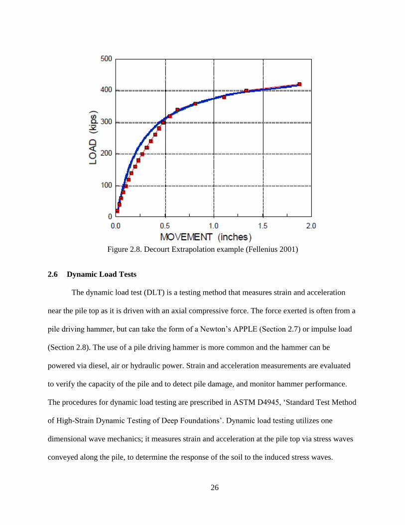
The Decourt Extrapolation (1999) is constructed similar to the Chin-Kondner

Extrapolation and Hansen methods; each load is divided by its corresponding settlement and

plotted against the applied load presented in Eqn.2.21 and illustrated in Figure 2.8. The results of

the Decourt Extrapolation are similar to the Chin-Kondner Extrapolation and allow projected

capacity to be determined as the SLT is in progress. The Hanson 80% Criterion, Chin-Kondner

Extrapolation, and the Decourt Extrapolation all have an equation that represents an ideal load

curve (Q) that compares with the ultimate load curves.

𝑄𝑢 = 𝐶2

𝐶1

Eqn.2.21

Where: Qu is the capacity or ultimate load, C1 is the slope of the straight line, and C2 is the y-

intercept of the straight line.

To illustrate the differences among the aforementioned methodologies, Bengt H.

Fellenius presented the graphs in Figures 2.4 through 2.8 in his presentation to the Deep

Foundation Institute in 2001. A SLT was performed on a 12 inch precast concrete pile and

various failure criteria were used to evaluate ultimate capacity.

Figure 2.4 which indicates an ultimate capacity of 375 kips. The DeBeer Yield Limit

produced an ultimate capacity of 360 kips in Figure 2.5. The Hansen 80% criterion produced an

ultimate capacity of 418 kips in Figure 2.6. Whereas the Chin-Kondner Extrapolation in Figure

2.7 gave an ultimate capacity of 475 kips and the Decourt Extrapolation in Figure 2.8 produced

an ultimate capacity of 474 kips. The example presented gave capacities which varied by 114

24

kips and serves to illustrate the uncertainty associated with reporting ultimate pile capacity if the

pile cannot be loaded to plunging failure. The Davisson Offset Limit criterion is one of the more

conservative methods to determine ultimate capacity and its ease of use through analysis has

increased its popularity among professionals.

Figure 2.4. Davisson Offset Limit example (Fellenius 2001)

Figure 2.5. DeBeer Yield Limit example (Fellenius 2001)

25

Figure 2.6. Hansen 80% criterion example (Fellenius 2001)

Figure 2.7. Chin-Kondner Extrapolation example (Fellenius 2001)

26

Figure 2.8. Decourt Extrapolation example (Fellenius 2001)

2.6 Dynamic Load Tests

The dynamic load test (DLT) is a testing method that measures strain and acceleration

near the pile top as it is driven with an axial compressive force. The force exerted is often from a

pile driving hammer, but can take the form of a Newton’s APPLE (Section 2.7) or impulse load

(Section 2.8). The use of a pile driving hammer is more common and the hammer can be

powered via diesel, air or hydraulic power. Strain and acceleration measurements are evaluated

to verify the capacity of the pile and to detect pile damage, and monitor hammer performance.

The procedures for dynamic load testing are prescribed in ASTM D4945, ‘Standard Test Method

of High-Strain Dynamic Testing of Deep Foundations’. Dynamic load testing utilizes one

dimensional wave mechanics; it measures strain and acceleration at the pile top via stress waves

conveyed along the pile, to determine the response of the soil to the induced stress waves.

27

Dynamic load testing can provide real time results, and is relatively inexpensive (Steele et al.

1990). Instrumentation for DLT requires accelerometers and strain gauges that are bolted,

welded, or glued onto the side of the pile near its top illustrated in Figure 2.9. The signals from

these transducers produce time traces of force and velocity for every hammer blow. A software

program is used to manipulate soil resistance and dynamic damping and quake values to produce

a calculated force curve that matches the measured force curve. This process is called signal

matching. Dynamic load testing is less reliable than static load testing due to the analysis not

providing a unique solution and the dependence on the user’s ability to model the system

accurately.

Figure 2.9. Strain gauge and accelerometer attached to a pile for dynamic testing

(GRL Engineers, Inc. 2014)

2.6.1 Dynamic Load Testing with Signal Matching

In 1964, the Ohio Department of Transportation initiated a research project at Case

Institute of Technology that explored the idea of using a dynamic approach to determine pile

capacity (Goble et al. 1975). The research effort used strain gages and recorded the data on high

28

speed oscillographs. This method was slow, recording only a few blows per pile, and was prone

to errors while converting analog signals to digital data during calibrations. In 1970 the portable

tape recorder replaced the oscillograph and eliminated the need for digital conversions. This

allowed for faster data collection, recording results for every blow of the hammer with more

accuracy.

Today, most dynamic testing is conducted with the use of the signal matching. Signal

matching is a type of high strain dynamic testing that measures strain and acceleration at the pile

top through strain gages and accelerometers attached to the pile. Electrical signals are

transmitted with wires or through wireless radios to a device which conditions the signals and

performs the signal matching analysis. Strain transducers measure the force while the

accelerometers measure the motion of the pile. The pile-soil system is modeled using the CAse

Pile Wave Analyses Program (CAPWAP) which attempts to find a tip and side resistance that

produces a force versus time signal which matches the measured data. Signal matching is useful

in measuring the activated soil resistance and distribution, along with the maximum compressive

and tensile stresses within the pile shaft, pile integrity, and hammer performance (Likins 1998).

CAPWAP is a signal matching software program offered by Pile Dynamics, Inc.

CAPWAP is based on the wave equation model which analyses the hammer-pile-soil system as a

series of elasto-plastic elements with damping characteristics (Alvarez et al. 2006). CAPWAP

predicts the side and toe resistance, as well as the total capacity of the pile (Pile Dynamics 2012).

The program uses the measured force based on the strain data collected and Hooke’s Law, to

give an expression of force (F) to be the product of strain (ε), the modulus of elasticity (E) of the

material, and the cross-sectional area (A) of the pile (F = εEA). The velocity is determined by

integrating the measured acceleration over time. CAPWAP performs an iterative process that

29

maintains dynamic equilibrium of the system with a calculated resistive force that is generated

by varying tip and side resistance and by manipulating the damping factors for the soil and pile.

An illustration of the force-time graph is presented in Figure 2.10 where the measured force in

the pile is compared to the calculated force as a function of time. This graph shows a good

signal match up to 40 ms, but would require more iterations to create a better fit the remainder of

the curve.

Figure 2.10. Example of CAPWAP signal matching (Bradshaw et al. 2006)

Dynamic load testing using signal matching can cost up to $25,000 to $45,000 per test

site with mobilization costs included (PDI 2013). A pile testing project for Milwaukee Stadium

documents the cost of signal matching at $3,000 per test (PDI 2002).

30

2.7 A Preferred Pile Load Evaluator (Newton’s APPLE)

The Newton’s APPLE loading system, illustrated in Figure 2.11, is large strain dynamic

testing system, named after Sir Isaac Newton’s second law of motion (Force = Mass x

Acceleration). The loading system is a rigid frame that allows a ram to freely drop from various

heights and has the ability to generate proof loads up to 400 tons (4000 kN) (GRL-PDI 2000).

This method measures force at the pile top and provides more accurate force values than from

strain transducers attached to concrete piles with questionable values for modulus of elasticity.

Figure 2.11. Newton’s APPLE loading system (PDI 2002)

31

2.8 Statnamic Load Testing

The statnamic load test was developed by Patrick Birmingham in 1989. It is based on

Newton’s second and third law of motion which state that force (F) is equal to mass (M) times

acceleration (A) (Force = MA) and that for every action there is an equal and opposite reaction.

Statnamic load testing is standardized by ASTM D7383, Standard Test Methods for Axial

Compressive Force Pulse (Rapid) Testing of Deep Foundations. It can be used as an alternative

to ASTM D1143 (static load testing in compression) or as a higher quality alternative to ASTM

D4945 (high strain dynamic testing). Statnamic load testing is a rapid load test which combines

the simple analysis of static testing with the efficiency and cost effectiveness of dynamic testing

(Hannigan et al. 2006). The impulse load is provided through the buildup of pressure in a heavy

cylindrical vessel which acts as a reaction mass that rests on top of the pile. A nitrocellulose

based explosive material used in shotgun shells is burned inside the cylinder at a rapid rate to

generate gas pressure (an explosion), as the pressure builds, it propels the reaction mass upward,

initiating a downward force applied to the pile top. The load generated can range from 10 kips

(44.5 kN) to 10,000 kips (44,482 kN). The set up time is a fraction of the cost and time of static

tests; the exception in this case is that reaction piles, reaction beam, and the hydraulic jack are

not required (Statnamic Load Testing 2012).

2.9 Case Study - A Comparison of SLT to DLT Capacity Values

The Caminada Bay Bridge project in Louisiana compares SLT and DLT performed on

production piles (Yoon et al. 2011). Static analyses were performed with the Tomlinson α-

Method for cohesive soils and the Norlund β-Method for cohesionless soils and resulted in a

target capacity of 1,129 kips, comparatively drawing on experience, it was projected that a

capacity of 1,219 kips was achievable. Wave equation analysis confirmed that the selected pile

32

with the chosen pile hammer could achieve pile resistance between 190 kips to 2,000 kips. Static

load testing (quick loading method) was conducted 27-days after the initial pile driving.

Dynamic load testing was conducted with signal matching at a 7-day restrike after the static load

test. Signal matching was performed at the end of drive (EOD), and at two beginning-of-restrike

(BOR) conditions. The result of the SLT, which was combined with internal strain gauge

monitoring indicated a plunging load of 558 kips. Using the load-settlement curve provided from

the SLT and the Davisson Offset Limit criteria, the ultimate capacity was determined to be 540

kips. The DLT (after static load test restrike) capacity using signal matching was 600 kips. All

load test data are summarized in Table 2.2. While the dynamic analysis over predicted the pile

capacity, the measured SLT and DLT results were within an acceptable range of ten percent

(10%). This evidence confirms SLT and DLT are comparable, and promotes the idea that

performing DLT on all installed piles can quantify the capacity and quality of the piles used in

foundation design.

Table 2.2 Pile capacity with time for static analysis, SLT, and DLT performed

on the Caminada Bay Bridge Project.

Pile Testing Capacity

(kips)

Static Analysis (Tomlinson and Norlund) 1,219

DLT - End of initial drive (EOD) 450

DLT - 7-day restrike 570

SLT - 27-days after initial pile driving (Plunging) 558

SLT - 27-days after initial pile driving (Davisson) 540

DLT - Restrike after static load test 600

2.10 Geotechnical Design Process and Reliability

Geotechnical engineering is a field where great uncertainty exists. These uncertainties are

prevalent in various empirical design methodologies, site characterization, soil behavior, and

33

construction quality (Paikowsky et al. 2004). Since the early 1800s, the Allowable Stress Design

(ASD), also known as working stress design, method was used to design foundations. In ASD,

the design load is compared to the nominal resistance with a factor of safety applied to the

resistance using Eqn. 2.22. An appropriate factor of safety was determined through engineering

experience to account for the uncertainties listed above, this apparent trial and error approach

lacked suitable support to quantify the reliability and performance of the resulting designs. Due

to the lack of a rational approach to assign factors of safety, this method often produces

conservative results that reflect highly over-designed and expensive foundations.

𝑄 ≤ 𝑄𝑎𝑙𝑙 = 𝑅𝑛

𝐹𝑆=

𝑄𝑢𝑙𝑡

𝐹𝑆

Eqn. 2.22

Where: Q is the design load, Qall is the allowable design load, Rn is the nominal resistance of the

element or the structure, FS is the factor of safety, and Qult is the ultimate geotechnical

foundation resistance.

Due to the desire for a more economical approach to design, Limit State Design (LSD)

was employed to address safety factor concerns, serviceability, and economic requirements

(Paikowsky et al. 2010, NCHRP 651). Additionally, LSD identifies the limit where the structure

fails to fulfill the purpose for which it was designed. There are two types of limit states when

referring to LSD, the ultimate limit state (ULS) considers the strength of the structure, and the

serviceability limit state (SLS) which considers the functionality and service requirements of a

structure for adequate performance under expected loading conditions (Paikowsky et al. 2010).

The ULS approach depends on the predicted loads and the ability of the structure to resist such

loads. The uncertainties that arise in design are quantified through probability based methods and

use a format called load and resistance factor design (LRFD). This method separates the

34

uncertainties due to load and the uncertainties due to resistance and ensures an acceptable margin

of safety through the application of probability theory. In the LRFD method, load factors (γ) are

applied to nominal loads to obtain a factored load. Likewise, resistance factors (ϕ), known as

strength reduction factors, are applied to the ultimate capacity (Coduto 2001).

The American Association of State and Highway and Transportation Officials

(AASHTO) LRFD Bridge Design Specifications recommends Eqn. 2.23 for strength limit state

in foundation design as:

𝑅𝑟 = 𝜙𝑅𝑛 ≥ ∑ 𝜂𝑖𝛾𝑖𝑄𝑖 Eqn. 2.23

Where: the factored resistance (Rr),the product of the nominal (ultimate) resistance (Rn) and its

resistance factor (ϕ) must be greater than or equal to the summation of loads (Qi) multiplied by

their corresponding load factors (γi) and a modifier (ηi) (AASHTO 2010). The modifier (ηi) is

taken as:

𝜂𝑖 = 𝜂𝐷𝜂𝑅𝜂𝐼 > 0.95 Eqn. 2.24

Where: ηD accounts for the ductility of the structure, ηR accounts for the redundancy in the

structure, and ηI is operational importance of the structure (AASHTO 2010).

The theory of LRFD can be illustrated through the use of probability density functions

(PDF) representing load (Q) and resistance (R) and their relation to the limit state function (g).

The limit state function (g) is defined by Eqn. 2.25 for a normal distribution of data and Eqn.

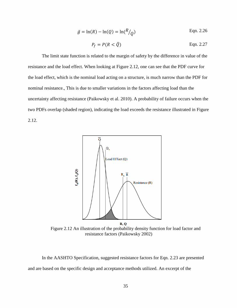
2.26 for a lognormal distribution of data. The probability of failure (Pf) is defined by Eqn. 2.27:

�̅� = 𝑅 − 𝑄 Eqn. 2.25

35

�̅� = ln(𝑅) − ln(𝑄) = ln (𝑅𝑄⁄ ) Eqn. 2.26

𝑃𝑓 = 𝑃(𝑅 < �̅�) Eqn. 2.27

The limit state function is related to the margin of safety by the difference in value of the

resistance and the load effect. When looking at Figure 2.12, one can see that the PDF curve for

the load effect, which is the nominal load acting on a structure, is much narrow than the PDF for

nominal resistance., This is due to smaller variations in the factors affecting load than the

uncertainty affecting resistance (Paikowsky et al. 2010). A probability of failure occurs when the

two PDFs overlap (shaded region), indicating the load exceeds the resistance illustrated in Figure

2.12.

Figure 2.12 An illustration of the probability density function for load factor and

resistance factors (Paikowsky 2002)

In the AASHTO Specification, suggested resistance factors for Eqn. 2.23 are presented

and are based on the specific design and acceptance methods utilized. An excerpt of the

36

Specification Table 10.5.5.2.3-1 (AASHTO 2010) is presented in Table 2.3 which gives

resistance factors ranging from 0.65 to 0.8 depending on the use of either SLTs or DLTs and the

number of load tests that are performed. Statistical analysis tools available range from the simple

averaging of values to more elaborate methods such as First Order Second Moment (FOSM),

First Order Reliability Methods (FORM), and the Monte Carlo Simulation (MCS).

Table 2.3 Excerpt for resistance factors for driven piles (AASHTO 2010)

2.11 Reliability and LRFD Design

In geotechnical engineering design, the probability that a structure will not fail can be

defined as the probability of failure (pf) or the level of reliability (1-pf) ,and is usually 99% or

higher. The reliability level in LRFD is often represented by the reliability index (β) presented in

Eqn. 2.28, which is the number of standard deviations (σ) separating the mean value (�̅�) load

from the origin on the PDF in Figure 2.13. Load and resistance factors are calculated and

adjusted to meet a target reliability index (βT) (Paikowsky et al. 2010).

37

𝛽 = 𝑚𝑔

𝜎𝑔=

(𝑚𝑅𝑁 − 𝑚𝑄𝑁)

√𝜎𝑄𝑁2 + 𝜎𝑅𝑁

2

=

ln [(�̅��̅�⁄ ) √(1 + 𝐶𝑂𝑉𝑄

2) (1 + 𝐶𝑂𝑉𝑅2)⁄ ]

√ln(1 + 𝐶𝑂𝑉𝑅2)(1 + 𝐶𝑂𝑉𝑄

2)

Eqn. 2.28

Where: mg is the mean of the nominal safety margin, σg is the standard deviation of the safety

margin defined by the limit state function g, mRN and mQN are mean of the natural logarithm of

the load and the resistance, 𝜎𝑄𝑁2 and 𝜎𝑄𝑁

2 are standard deviations of the natural logarithm of the

load and the resistance, �̅� and �̅� are the mean of the load and the resistance, and COVQ and

COVR are the coefficient of variation of the load and resistance assuming a normal distribution

(Paikowsky et al. 2010).

Figure 2.13 The performance function for a normal distribution (g(R,Q)) demonstrating the

margin of safety (pf) and its relation to the reliability index, β (σg = standard deviation of g)

(Paikowsky et al. 2010)

38

2.11.1 Statistical Terms

The methods used to quantify the state function include: First Order Second Moment,

First Order Reliability Method, and the Monte Carlo Simulation. These methods are an integral

part of determining the resistance factor. However, prior to explaining these methods, it is

essential to define the common statistical parameters used in each method. The common

parameters are mean, standard deviation, sample variance, and coefficient of variation. The mean

(μ) is the average value of the sample and calculated with Eqn. 2.29:

𝜇 = 1

𝑛∑ 𝑥𝑖

𝑖

Eqn. 2.29

The standard deviation (σ) indicates how much variation there is from the mean and calculated

with Eqn. 2.30:

𝜎 = √1

𝑁 − 1∑(𝑥𝑖 − �̅�)2

𝑖

Eqn. 2.30

The sample variance (σ2) is a measure of how spread out the values are and calculated using Eqn.

2.31:

𝜎2 =1

𝑁 − 1∑(𝑥𝑖 − �̅�)2

𝑖

Eqn. 2.31

The coefficient of variation (COV) measures the normalized dispersion of a sample population

and is determined using Eqn. 2.32, which enables a comparison of several data sets (Miller et al.

1985):

𝐶𝑂𝑉 = 𝜎

𝜇

Eqn. 2.32

39

2.11.2 First Order Second Moment (FOSM)

First Order Second Moment (FOSM) is a closed form solution and a probabilistic

reliability method that produces a resistance (ϕ) factor for a given reliability index (β). It is based

on the lower order terms from a Taylor series expansion of the performance function to

approximate the variance of the performance function (Baecher et al. 2003). The FOSM is a

first-order expansion about the mean value and a linear approximation of the second moment

(the variance) (Patev 2010). First Order Second Moment requires the limiting state function, the

mean, and standard deviations of the design parameters. FOSM has had a presence in

geotechnical engineering since 1969 when it was originally proposed by C. A. Cornell. It was

subsequently used by Barker et al. (1991) for NCHRP Report 343 titled “The calibration of

geotechnical resistance factors using closed form solutions”.

The limit state occurs when the state equation equals zero, g(x) = 0, a value greater than

zero is considered a safe state, g(x) > 0, and a value less than zero is at considered a failure state,

g(x) < 0. The geotechnical resistance (ϕ) factors can be derived from Eqn. 2.23 by setting η to

one and following the procedure described in Becker et al. (1991) and FHWA (2001):

ϕRn ≥ ∑ γiQi Eqn. 2.33

From which:

ϕ ≥ ∑ γi

Qi

Rn

Eqn. 2.34

The nominal resistance (Rn) is replaced by the mean value divided by the bias factor, �̅�/λR,

which gives:

40

ϕ ≥ λR ∑ γi

Qi

R̅

Eqn. 2.35

Using the lognormal form of Eqn. 2.28, the mean value of the resistance (�̅�):

�̅� =

�̅�𝑒𝑥𝑝 {𝛽√ln(1 + 𝐶𝑂𝑉𝑅2)(1 + 𝐶𝑂𝑉𝑄

2)}

√(1 + 𝐶𝑂𝑉𝑄2) (1 + 𝐶𝑂𝑉𝑅

2)⁄

Eqn. 2.36

Then substituting �̅� into Eqn. 2.35 and replacing β with the target reliability (βT) the expression

for ϕ becomes:

ϕ =

λR(∑ γiQi)√1 + COVQ

2

1 + COVR2

Q̅exp {βT√ln[(1 + COVR2)(1 + COVQ

2)]}

Eqn. 2.37

Where: λR is the resistance bias factor which in the context of pile capacity is the mean of the

ratio of measured pile capacity over predicted pile capacity, γi is the load factor for the specific

type of load, Qi is the specific type of load applied (dead load, live load, environmental load,

etc.), �̅� is the mean of the load and subsequently referred to as λQ, COVQ is the coefficient of

variation of the load, COVR is the coefficient of variation of the resistance, and βT is the target

reliability index (Paikowsky 2004). Eqn. 2.37 can be restated in a simpler form when only the

dead and live loads are considered as was presented in the NCHRP Report 507 and illustrated in

Eqn. 2.38 (Paikowsky 2004):

ϕ =

λR (γDQD

QL+ γL) √

(1 + COVQD

2 + COVQL

2 )

1 + COVR2

(λQD

QD

QL+ λQL

) exp {βT√ln[(1 + COVR2)(1 + COVQD

2 + COVQL

2 )]}

Eqn. 2.38

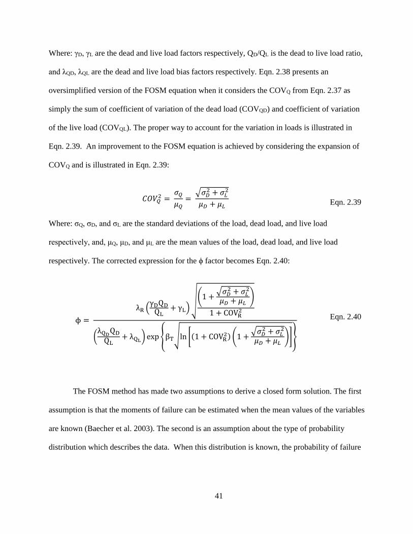
41

Where: γD, γL are the dead and live load factors respectively, QD/QL is the dead to live load ratio,

and λQD, λQL are the dead and live load bias factors respectively. Eqn. 2.38 presents an

oversimplified version of the FOSM equation when it considers the COVQ from Eqn. 2.37 as

simply the sum of coefficient of variation of the dead load (COVQD) and coefficient of variation

of the live load (COVQL). The proper way to account for the variation in loads is illustrated in

Eqn. 2.39. An improvement to the FOSM equation is achieved by considering the expansion of

COVQ and is illustrated in Eqn. 2.39:

𝐶𝑂𝑉𝑄2 =

𝜎𝑄

𝜇𝑄=

√𝜎𝐷2 + 𝜎𝐿

2

𝜇𝐷 + 𝜇𝐿 Eqn. 2.39

Where: σQ, σD, and σL are the standard deviations of the load, dead load, and live load

respectively, and, μQ, μD, and μL are the mean values of the load, dead load, and live load

respectively. The corrected expression for the ϕ factor becomes Eqn. 2.40:

ϕ =

λR (γDQD

QL+ γL)

√(1 +

√𝜎𝐷2 + 𝜎𝐿

2

𝜇𝐷 + 𝜇𝐿)

1 + COVR2

(λQD

QD

QL+ λQL

) exp {βT√ln [(1 + COVR2) (1 +

√𝜎𝐷2 + 𝜎𝐿

2

𝜇𝐷 + 𝜇𝐿)]}

Eqn. 2.40

The FOSM method has made two assumptions to derive a closed form solution. The first

assumption is that the moments of failure can be estimated when the mean values of the variables

are known (Baecher et al. 2003). The second is an assumption about the type of probability

distribution which describes the data. When this distribution is known, the probability of failure

42

and the reliability index can be computed (Baecher et al. 2003). While closed form solutions are

easy to apply, they can be too simplistic for foundation design (Phoon et al. 2003).

2.11.3 First Order Reliability Method (FORM)

The First Order Reliability Method (FORM) was first proposed for use in 1974 by

Hasofer and Lind (Baecher et al. 2003) to address the limitations of the FOSM by identifying a

geometric interpretation of the reliability index (β) and not relying on assumptions or

extrapolations. The reliability index (β) is the measured distance in dimensionless space between

the mean of the limit state function or performance function as �̅� = R-Q and the failure function

(g = 0) (Baecher et al. 2003). The First Order Reliability Method is the preferred method to

calibrate resistance factors (Baecher et al. 2003) and has been used in structural design for years.

It provides an estimate of the probability of failure (pf) as expressed in Eqn. 2.41:

pf = Φ(−β) Eqn. 2.41

Where: Φ( ) is the cumulative distribution function of the standard normal distribution

(Paikowsky 2004). The First Order Reliability Method is an iterative process that allows for the

calculation of partial safety factors for load and resistance factors with respect to a target level of

reliability (βT). It requires the first and second moment (mean and variance) information for the

load and resistance factors and an assumed shape for the distribution (Paikowsky et al. 2010).

The FORM assumes an initial design point (𝑥𝑖∗) on the failure surface. The design point is

usually the point on the failure surface closest to the mean point, the highest point on the

probability density curve (Phoon et al. 2003). This assumption creates a situation that is

constrained, nonlinear, and requires minimization (Maier 2001). The design point is transformed

43

into standard normal variable (𝑥′𝑖∗) which is dimensionless with zero mean and a standard

deviation of one using Eqn. 2.42:

𝑥′𝑖∗ =

𝑥𝑖∗ − 𝜇𝑋𝑖

𝜎𝑋𝑖

Eqn. 2.42

Where: 𝜇𝑋𝑖is the mean value of the random variable X and 𝜎𝑋𝑖

is the standard deviation of the

random variable for the distribution (Paikowsky et al. 2004). The random variable (X) is the

vector of the difference between the strength and load variables. An equivalent normal

distribution at the design point may be necessary for non-normal distributions, such as lognormal

distributions. The equations needed to convert a non-normal mean and standard deviation to an

equivalent mean and equivalent standard deviation are illustrated in Eqn. 2.43 and Eqn. 2.44

(Phoon et al. 2003):

μXN = x∗ − Φ−1(Fx (x∗)σX

N) Eqn. 2.43

𝜎𝑋𝑁 =

ϕ (Φ−1(𝐹𝑋(𝑥∗)))

𝑓𝑋(𝑥∗) Eqn. 2.44

Where: 𝜇𝑋𝑁 is the mean of the equivalent normal distribution, 𝜎𝑋

𝑁 is the standard deviation of the

equivalent normal distribution, 𝐹𝑋(𝑥∗) is the original cumulative distribution function (CDF) of

Xi evaluated at the design point, 𝑓𝑋(𝑥∗) is the original PDF of Xi evaluated at the design point,

and ϕ( ) is the PDF of the standard normal distribution (Paikowsky 2004). Once the necessary

equivalent moments are established the random variable can be used to minimize the function:

𝑥′𝑖∗ = 𝛼𝑖

∗𝛽 Eqn. 2.45

Where: 𝛼𝑖∗ is the directional cosine expressed in Eqn. 2.46 and normalize to a unit vector:

44

𝛼𝑖∗ =

(𝜕𝑔𝜕𝑥𝑖

′)∗

√∑ (𝜕𝑔𝜕𝑥𝑖

′)∗

2𝑛𝑖=1

𝑓𝑜𝑟 𝑖 = 1, 2, … 𝑛 Eqn. 2.46

Where:

(𝜕𝑔

𝜕𝑥𝑖′)

∗

= (𝜕𝑔

𝜕𝑥𝑖)

∗

𝜎𝑋𝑖

𝑁 Eqn. 2.47

The reliability index (β) can then be determined using Eqn. 2.48 once the variables 𝛼𝑖∗, μX𝑖

N , and

σX𝑖

N are known:

𝑔[(μX1

N − 𝛼𝑋1

∗ σX1

N 𝛽)] ⋯ (μX𝑛

N − 𝛼𝑋𝑛

∗ σX𝑛

N 𝛽) = 0 Eqn. 2.48

A new design point is obtained using Eqn. 2.49 with the β found in Eqn. 2.45:

𝑥𝑖∗ = μX𝑖

N − 𝛼𝑖∗σX𝑖

N 𝛽 Eqn. 2.49

These procedures are repeated until calculated values of β converge to a common value. The

mean value of the resistance (μ) and the design point (𝑥𝑖∗) are used to calculate the resistance

factor (ϕ) (Paikowsky 2004):

ϕ = R∗

μR=

xR∗

μXR

Eqn. 2.50

The difference between FOSM and FORM is that FORM allows the failure function to

take any shape as long as the failure criterion remains constant, meaning the safety factor equates

to one, or the margin of safety equates to zero (Baecher et al. 2003).

45

2.11.4 Monte Carlo Simulation

Monte Carlo Simulation (MCS) is a form of experimental mathematics that provides

probabilistic or deterministic solutions to problems. The MCS was considered a strong research

tool in 1944 during the era of the Second World War (Hammersley et al. 1964). Since then the

method has been refined and proper applications have been identified that make it a strong tool

for solving deterministic problems. Prior to the refinement of the MCS method, researchers

attempted to use it as a solution technique for all problems (Hammersley et al. 1964) and

discovered the MCS had inefficiencies and some problems modeling certain situations. The use

of the MCS regained popularity once specific cases that would benefit from this type of analysis

were identified and variance reducing techniques made the computations more efficient

(Hammersley et al. 1964).

The MCS applications are ideal tools for problems where an exact result is unattainable

through normal sampling techniques. It is useful in modeling events with great uncertainty, or in

solving problems with multiple sources of uncertainty. The MCS lends itself to complex

multidimensional integrals and to problems where realism is modeled with complex and

involved problem descriptions (Rubinstein 1981). The MCS method has become AASHTO’s

preferred calibration tool and is recommended for all AASHTO related calibrations of LRFD

factors (Paikowsky et al. 2010).

As in the previous FORM, the MCS attempts to estimate the probability of failure. The

MCS method generates random values of load (Q) and resistance (R) based on the mean, COV,

and distribution of the sample. The limit state function, g = Q-R or g = ln(Q/R), is formed with

the random values and evaluated for failure. Failure is defined when g < 0. A predetermined

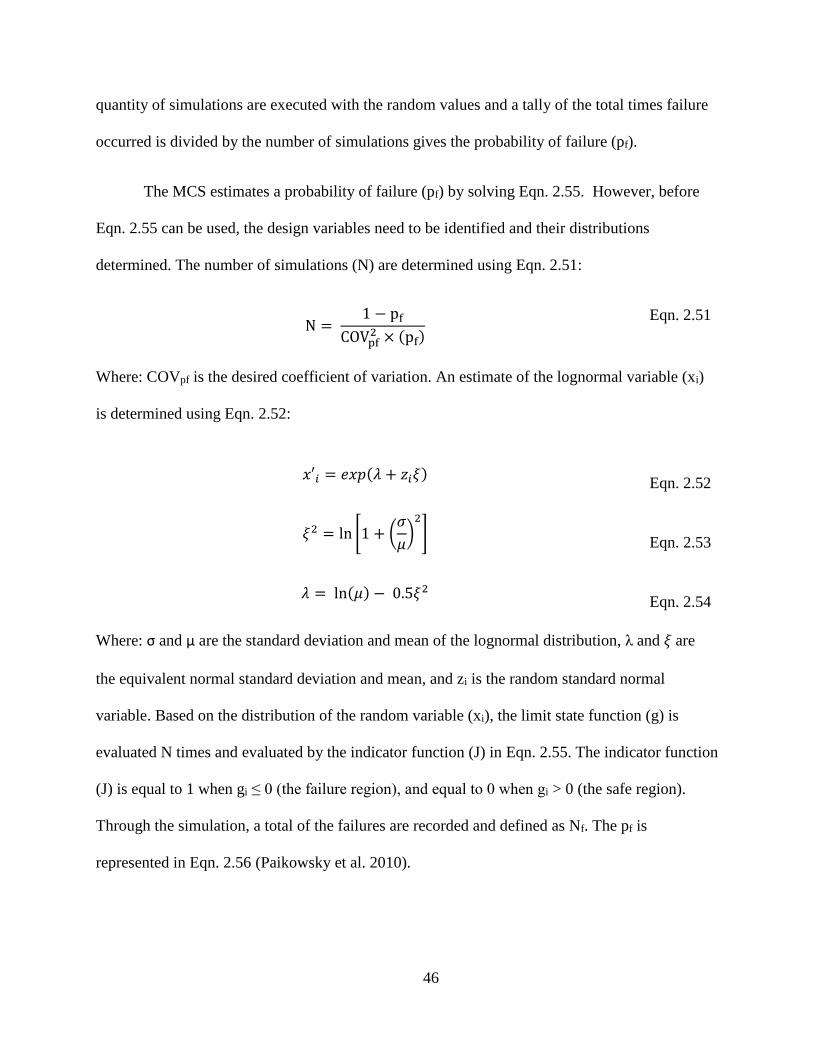
46

quantity of simulations are executed with the random values and a tally of the total times failure

occurred is divided by the number of simulations gives the probability of failure (pf).

The MCS estimates a probability of failure (pf) by solving Eqn. 2.55. However, before

Eqn. 2.55 can be used, the design variables need to be identified and their distributions

determined. The number of simulations (N) are determined using Eqn. 2.51:

N = 1 − pf

COVpf2 × (pf)

Eqn. 2.51

Where: COVpf is the desired coefficient of variation. An estimate of the lognormal variable (xi)

is determined using Eqn. 2.52:

𝑥′𝑖 = 𝑒𝑥𝑝(𝜆 + 𝑧𝑖𝜉) Eqn. 2.52

𝜉2 = ln [1 + (𝜎

𝜇)

2

] Eqn. 2.53

𝜆 = ln(𝜇) − 0.5𝜉2 Eqn. 2.54

Where: σ and μ are the standard deviation and mean of the lognormal distribution, λ and 𝜉 are

the equivalent normal standard deviation and mean, and zi is the random standard normal

variable. Based on the distribution of the random variable (xi), the limit state function (g) is

evaluated N times and evaluated by the indicator function (J) in Eqn. 2.55. The indicator function

(J) is equal to 1 when gi ≤ 0 (the failure region), and equal to 0 when gi > 0 (the safe region).

Through the simulation, a total of the failures are recorded and defined as Nf. The pf is

represented in Eqn. 2.56 (Paikowsky et al. 2010).

47

pf = P(g ≤ 0) =1

N∑ J[gi ≤ 0]

N

i−1

Eqn. 2.55

pf =Nf

N

Eqn. 2.56

Where: N is the number of simulations carried out (Paikowsky et al. 2010). The reliability index

(β) is then calculated with Eqn. 2.41 rearranged to give Eqn. 2.57:

β = Φ−1(1 − pf) Eqn. 2.57

2.12 Summary

The adoption of reliability concepts, namely LRFD, in geotechnical engineering has

attempted to bridge the gap between structural design and foundation design. The conservative

factors of safety used in ASD are steadily being replaced by load and resistance factors that

better classify the uncertainties related to ultimate capacity determination. Static load testing is a

full scale load test that measures the actual capacity of a pile and costly to perform, whereas,

dynamic load testing predicts the pile capacity and can be more economical. The load test

capacities collected within this study will allow for a comparison of the testing methods whose

parameters are dependent on the ratio of SLT to DLT and the respective coefficient of variation.

The reliability analyses, First Order Second Moment, First Order Reliability Method, and the

Monte Carlo Simulation, are useful in determining suitable resistance factors, given the pile

driving condition.

48

3 Methodology

3.1 Introduction

In order to compare and analyze the relationship between pile capacities obtained from

Static and Dynamic load testing, it was necessary to understand all the conditions under which

the tests were performed. Information regarding the soil profile the piles were driven into, the

pile material type and geometry to establish design capacities, were necessary to group load

cases into special sub-categories. The particulars of the driving operation which might include

information on pre-boring, jetting or delays in driving, as well as information about testing

conditions, such as the delay between driving and testing, might be useful in discerning the

reasons for anomalous data. The governing standards and practices of the agencies performing

the tests may also affect the results of the test. Essentially, all information about a load test is

considered important in some manner when establishing a load test database. Once the data is

collected, preliminary statistical evaluations were performed to identify any correlative trends

and the general scatter of the relationship between dynamic and static capacities. Preliminary

information on the distribution of the data may also be developed to inform the reliability

analyses that will be used to establish resistance factors for various categories of pile load cases.

The pile load test cases found suitable for analysis in this study consisted of those for

which the following information was available: capacity from a static load test (SLT) carried to

at least 2.0 times the design load, capacity from a dynamic load test (DLT) at end-of-driving

(EOD) and/or at the beginning-of-restrike (BOR), established with signal matching analysis. The

piles should have been driven in a landform similar to that found in Arkansas. Sufficient

information should be available to classify the soil profile in which the pile was driven. The pile

itself was one of four pile types: Precast or Precast-Prestressed Concrete Piles, H-Piles, or Pipe

49

Piles. Of the more than 1000 pile load cases investigated, only 138 piles were found that met all

of these criteria.

3.1 Database Development

The preliminary step in gathering the data for this study was reviewing case studies and

reports from Departments of Transportation in neighboring states where both static (SLT) and

dynamic load tests (DLT) had been performed, and where soils information was provided. The

primary states of interest were Louisiana, Missouri, and Alabama. The state of Arkansas itself

had no load cases where static load testing had been conducted.

3.1.1 Determining Soil Profile

The objective of the data search was to find load tests that were performed in soil types

similar to those found in Arkansas. Arkansas has two distinct regions, as illustrated in Figure 3.1,

where the soil profile can vary: the highlands in the northwest and the lowlands in the south and

east. The highland region consists of sandstone, shale, limestone, thin layers of unconsolidated

clays, sands, and gravel (residual soils). The lowlands consist of unconsolidated clays, sands,

gravel of the Quaternary Period, poorly consolidated deposits of clay, silt, limestone, and lignite

of the Tertiary Period (AGS 2012). Once a load tests had been identified, the geology of the area

was examined to accept or reject the case based on the soils present in Arkansas.

50

Figure 3.1. The geology of Arkansas (AGS 2012)

Using the pile driving records, or the information provided in the DOT reports, soil

profiles were broken into three major categories; clay, sand and mixed. The designation of a

soil profile was determined by using the 70% rule. The 70% rule considers the soil types along

the length of the pile. The soil type which represents 70% or greater of the pile length is

considered to be the dominating soil type that would be evaluated for friction piles (pipe and

PPC piles). When considering the H-Piles, the soil type relevant to end bearing capacities was

ideally the soil type located at the pile tip. For piles where detailed driving records or bore log

data were available, the soil type was classified accordingly using information from these

records. When these records were not present, the soil type was classified as recorded in the

initial report. For example, if 72% of the soil along the side of a pile consisted of clay or clayey

soil, the recorded soil profile would be clay. Similarly, if more that 70% of the soil along the pile

side were sand or sandy soil the profile would be recorded as sand. If two soil types are present,

with no clear majority, the soil profile would be considered mixed. Soil type was characterized in

51

accordance with the Unified Soil Classification System (USCS). The 70% rule could also be

interpreted as the soil type from which the pile derived 70% or more of its capacity. In fact, the

second interpretation of the 70% rule would be preferable when classifying soil type, but

sufficient strength information was not available to perform this type of classification for a

number of the piles in the database.

3.1.2 Louisiana Load Cases

The report titled “Calibration of Resistance Factors Needed in the LRFD Design of

Driven Piles” (Abu-Farsakh et al. 2009) was prepared for the Louisiana Department of

Transportation and Development (LADOTD). The report presented information on SLT, DLT

and Cone Penetration Testing (CPT) for 53 Precast-Prestressed-Concrete (PPC) piles tested to

failure. The load-settlement information from SLT was evaluated using the Davisson Offset

criterion for piles with diameter less than 24 inches and the modified Davisson Offset method for

piles with diameter more than 24 inches. The DLT program employed signal matching at both

EOD and BOR, with BOR testing taking place 14 days after driving. Soil profiles were

characterized using CPT soundings and soil borings. Of the 53 pile load cases described in the

report, 13 piles met the criteria for inclusion in the database by having both the SLT and DLT

values recorded and the necessary soil profile information.

The soil deposits in the State of Louisiana are made up of alluviul, lacuastrine and coastal

deposits of the Mississippi Embayment. Louisiana is divided into two main regions: the northern

Louisiana region, and the southern Louisiana region. Soils in the northern Louisiana region are

of the Tertiary Period, while the soils in the southern Louisiana region are of the Quaternary and

Tertiary Period (DOI 2008). Northern Louisiana and Eastern and Southern Arkansas have similar

52

soil profiles therefore piles driven in Louisiana were determined to be acceptable for inclusion in

the database.

3.1.3 Missouri Load Cases

Case studies from the Missouri Department of Transportation (MODOT) reports did not

meet the criteria for inclusion into the data base. The report only contained signal matching

predicted capacities. Though the MODOT report proved fruitless, a driving record was obtained

for a pile driven in 2011. The single pipe pile was predrilled five feet in a predominately clay soil

type. Dynamic load testing was conducted at EOD and at BOR with a 7 day waiting period.

Static load testing was performed nine days after driving with the pile being loaded to failure

according to the Davison Offset criterion (1972).

Missouri has four geologic regions: the Ozarks, Western Plains, Glaciated Plains, and

Southeast Lowlands. The pile of interest was driven in the Glaciated Plains region that has a mix

of clay, silt, sand, and rock fragments. The Glaciated Plains region is of the Pennsylvanian and

Mississippian age with Quaternary formations are similar to those in North and Northwest

Arkansas.

3.1.4 Alabama Load Cases

Data from Alabama was retrieved from a report titled ‘Evaluation of Load Tests for

Driven Piles for the Alabama Department of Transportation’ (Hill 2007), where 30 projects were

selected from the Alabama Department of Transportation database. Piles included in this study

were PPC piles and steel H-piles that were tested statically and dynamically using signal

matching. These piles were not loaded to failure, as the loading for the SLT was only to 2.0 or

3.0 times the design load. Load-settlement graphs from the project indicate that only one pile

53

was loaded to plunging failure. The load-settlement curves for the remaining piles suggest that

the reported SLT capacities were not those at plunging failure and simply represent the highest

load the pile was subjected to. This was typically 2.0 to 3.0 times the anticipated design load.

Dynamic load tests were carried out using signal matching for EOD conditions and BOR testing

were conducted on some of the piles with waiting periods ranging from 30 minutes to 60 days.

The soil profiles were constructed from boring log data and the 70% rule was implemented to

classify the soil type.

Alabama is made up five differing regions: Interior Low Plateau, Cumberland

Plateau, Valley and Ridge, Piedmont, and the Coastal Plains. The region of interest is the Coastal

Plains where all but one of the piles was tested. The Coastal Plains region consists of the

Mesozoic and Cenozoic Period, with sediments of gravels, sands, silts, and clays. This region is

similar to that found in eastern and southern Arkansas.

3.2 Other Data from Literature

3.2.1 WSDOT

The Washington State Department of Transportation (WSDOT) embarked on an effort to

calibrate resistance factors for a state-developed pile driving formula in a report titled

‘Development of the WSDOT Pile Driving Formula and Its Calibration for Load and Resistance

Factor Design (LRFD)’ (Allen 2005). Pile load test data from Paikowsky et al. (2004) database

was used to develop a hammer efficiency factor for use in the WSDOT pile driving formula. The

database included SLT and DLT data for 141 test piles at varying locations around the world.

The soil profiles were identified along the pile length for friction piles and at the pile tip for end

54

bearing piles. A total of 59 records were gathered from this report with soil profiles similar to

those found in Arkansas.

3.2.2 PILOT - IOWA

PILOT (PIle LOad Test) is a database developed for the state of Iowa. It is modeled after

the Federal Highway Administration’s (FHWA) Deep Foundation Load Test Database (DFLTD)

which has 1500 records of load test data from over 850 sites around the world. PILOT contained

274 SLT data with accompanying DLT and in-situ soil information. The types of piles in the

study were H-steel, monotube, pipe, timber, and concrete piles. Of the 274 pile load tests

considered, 12 piles (PPC Piles and H-Piles) met the criterion necessary to be included in this

analysis: SLT evaluated by the Davisson Offset criterion and DLT from EOD testing conditions.

3.2.3 FHWA - Central Artery/Tunnel (CA/T) Project, Boston, Massachusetts

The Central Artery/Tunnel (CA/T) project was considered one of the largest and most

complex highway projects in the United States (Bradshaw et al. 2006). The project took place

between 1991 and 2005, where 15 pile load tests were performed for evaluation. The piles were

precast prestressed concrete (PPC) or pipe piles and were driven into loamy soils, similar to

those found in southeast Arkansas. Loamy soils are a mixture of sands, silts, and clays

(Bradshaw et al. 2006). Dynamic load testing (ASTM D4945 2008) with signal matching was

conducted at both EOD and at BOR after a 12 to 36 hour waiting period. Static load tests (ASTM

D1143 2007) were carried to 2.0 to 2.25 times the required allowable axial capacities. The load

test reported met the criterion of having SLT, DLT, soils information and being a PPC pile.

55

3.3 Data Analysis

After eliminating load tests that did not meet the initial screening criteria, 138 load tests

remained in this study. The load tests were characterized by soil and pile type, then assigned to

groups as detailed in Chapter 4. An initial scatter plot of capacities measured using SLT, to

capacities predicted using DLT at EOD was created. The scatter plot was then fitted with a

regression line that implemented robust regression with iterative least square fitting techniques.

The next step was to calculate the ration of Qmeasured/Qpredicted from the raw SLT and DLT at

EOD capacities that would be used in further analyses to determine the distribution of the sample

population by the probability density function (PDF) and cumulative distribution function

(CDF). The CDF was often used to determine the distribution of the sample. The selection of the

appropriate mathematical distribution was further confirmed by the execution of the goodness-

of-fit test, in this case, the Chi-Square Test was used to accept or reject the PDF and CDF given

a hypothesis. A confidence interval (CI) of 95% was applied to the selected CDF using the

Inverse Fisher Matrix, bounding the data points and identified any points that fell outside the CI.

Once the distribution was decided upon, parameters of the mean bias, which was the mean of the

Qmeasured/Qpredicted of the sample, and the coefficient of variation (COV) applicable to the

distribution, were used in further reliability analysis. These analyses consist of the First Order

Second Moment, First Order Reliability Method, and the Monte Carlo Simulation. The software

programs used to perform these analyses were Microsoft Excel® and ReliaPile. ReliaPile is a

program based in MATLAB and was developed by Joseph Jabo, a Ph.D. candidate at the

University of Arkansas, Fayetteville, Arkansas.

56

3.3.1 Regression Analysis

Linear regression was carried out on the capacity values in the database by separating the

piles into subgroups by pile and soil type and plotting SLT capacity versus DLT capacity. The

best fit line of the data is the line that provides a minimum error (minimum distance) between the

data points and the regression line. The dependent DLT values were plotted on the y-axis, while

the corresponding independent SLT values were plotted on the x-axis. This type of analysis

allowed any trends to emerge as the points scatter about the line of equality (LOE). Any outlying

data point would be identified and investigated to possibly ascertain the reason it might be an

outlier.

3.3.2 Robust Regression and Iterative Least Squares Fitting Techniques

Least square fitting provides a best fit model function to describe the data by minimizing

the sum of the squares of the data point offsets to their perpendicular points on a curve described

by the model function. However, this technique is sensitive to outlying data points that may have

a large influence on the regression function (Heiberger et al. 1992). Because data in the

collected set of pile load tests contained data points that could be considered outliers, modified

fitting techniques were used to account for outlying data. Throughout the analysis of the data, a

technique called Robust Regression and Iterative Least Squares Fitting is used to accurately

represent the data and minimize any effect outliers may have on the data (Heiberger et al. 1992).

Robust regression assigns a weight to the data points and iteratively adjusts the weighting

function using least squares. While there are many weighting functions available in the literature,

the bisquare function, with the default tuning constant of 4.685 was used. During the first

iteration, the weight assigned is usually estimated using unweighted least squares. As iterations

continue the weights are reassigned to the data points, applying lower weights to points further

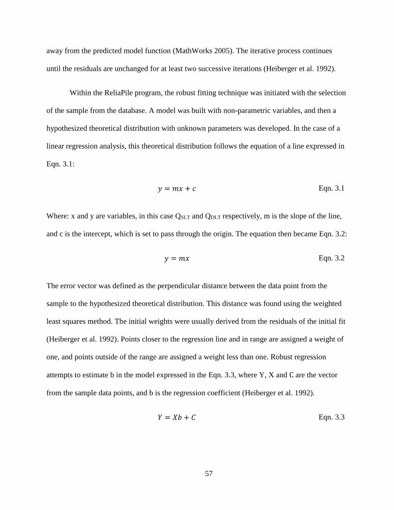
57

away from the predicted model function (MathWorks 2005). The iterative process continues

until the residuals are unchanged for at least two successive iterations (Heiberger et al. 1992).

Within the ReliaPile program, the robust fitting technique was initiated with the selection

of the sample from the database. A model was built with non-parametric variables, and then a

hypothesized theoretical distribution with unknown parameters was developed. In the case of a

linear regression analysis, this theoretical distribution follows the equation of a line expressed in

Eqn. 3.1:

𝑦 = 𝑚𝑥 + 𝑐 Eqn. 3.1

Where: x and y are variables, in this case QSLT and QDLT respectively, m is the slope of the line,

and c is the intercept, which is set to pass through the origin. The equation then became Eqn. 3.2:

𝑦 = 𝑚𝑥 Eqn. 3.2

The error vector was defined as the perpendicular distance between the data point from the

sample to the hypothesized theoretical distribution. This distance was found using the weighted

least squares method. The initial weights were usually derived from the residuals of the initial fit

(Heiberger et al. 1992). Points closer to the regression line and in range are assigned a weight of

one, and points outside of the range are assigned a weight less than one. Robust regression

attempts to estimate b in the model expressed in the Eqn. 3.3, where Y, X and C are the vector

from the sample data points, and b is the regression coefficient (Heiberger et al. 1992).

𝑌 = 𝑋𝑏 + 𝐶 Eqn. 3.3

58

The process of least squares was implemented by taking the independent variable, SLT capacity,

and estimating y given the x variable, which gives an unknown b. This estimation was repeated

at each data point and a collection of variables were analyzed for the error. The error vector (R)

was computed using Eqn. 3.4 and minimized by applying the condition in Eqn. 3.5, and n is the

number of data points:

𝑅 = (𝑦1 − 𝑏𝑥1, 𝑦2 − 𝑏𝑥2, … , 𝑦𝑛 − 𝑏𝑥𝑛 ) Eqn. 3.4

𝜕𝑅

𝜕𝑦𝑖= 0, 𝑖 = 1, 2, … , 𝑛

Eqn. 3.5

The sum of squares for the first iteration was made with an unweighed weighting function (w)

illustrated in Eqn. 3.6:

|𝑅|2 = ∑ 𝑤𝑖(𝑦𝑖 − 𝑏𝑥𝑖)2

𝑛

𝑖=1

, 𝑖 = 1, 2, … , 𝑛 Eqn. 3.6

As the robust fitting technique continued, with each iteration the weighting functions were

revised. This process continued until b converged to a constant value.

3.3.3 Probability Density Function (PDF)

Determination of the sample distribution type is an important step in developing the

parameters for use in the reliability methods. To do this the ration of measured (SLT) to

predicted (DLT) capacities are separated into bins representing small ranges in the ration values.

Then a histogram of the number of occurrences of the ration in a given bin was plotted against

the value of the bin in ascending order. A plot of various theoretical probability density

functions is then superimposed on the histogram to visually determine the distribution which

more closely fits the data. The probability density function (PDF) describes the frequency at

59

which a variable appears in a distribution. It is defined as a continuous function (X), which is the

Qmeasured/Qpredicted variable, by Eqn. 3.7 for a normal distribution and Eqn. 3.8 for a

lognormal distribution. The ration of the measured capacities and the predicted capacities are

ordered in ascending order and represent the variable (X) in Eqn. 3.7 and Eqn. 3.8 (Kroese et al.

2011):

𝑓(𝑥; 𝜇, 𝜎) = 1

𝜎√2𝜋𝑒−

12

(𝑥−𝜇

𝜎)

2

Eqn. 3.7

𝑓(𝑥; 𝜇, 𝜎) = 1

𝑥𝜎√2𝜋𝑒

−(𝑙𝑛(𝑥)−𝜇)2

2𝜎2 , 𝑥 > 0 Eqn. 3.8

The standard deviation of the sample population is represented by σ, and μ is the mean of the

sample population. Both equations were used to create the theoretical density function from the

sample statistics. The resulting curves were plotted with frequency on the y-axis and the ration

Qmeasured/Qpredicted on the x-axis. The curve that best fit the data (plotted in the histogram)

was visually chosen as the frequency distribution.

3.3.4 Cumulative Probability Function (CDF)

The cumulative distribution function (CDF) describes the value of the state function, in

this case the ration of measured to predicted capacity, in terms of the probability the that random

values from the population will be less than a given point on the cumulative distribution function

(Miller et al. 1985). These probabilities range between zero and one. The measured capacity,

(Qm), divided by predicted capacity, (Qp), are plotted in ascending order against the cumulative

frequency of occurrence. The probability of occurrence of values of this ration were calculated

using i/(n+1), where i is the rank of each data point when sorted, and n is the total number of

points in the sample. Both normal and lognormal distributions were analyzed using the

60

respective normal or lognormal variables. The resulting curves provided a more definitive way to

determine if the sample was normally or lognormally distributed, when PDF curves were not

conclusive. The mean (μ) and standard deviation (σ) were recorded for the selected distribution.

The COV of the capacity rations were then calculated and used to determine the resistance (ϕ)

factors by FOSM, FORM, and MCS.

3.3.5 Fisher Information Matrix and Confidence Interval

The approach to determine the confidence interval (CI) in the ReliaPile program employs

the inverse of the Fisher Information Matrix. The Fisher Information Matrix measures how much

information is known about a parameter by estimating the standard errors (Neale et al. 1997),

and was used when determining the confidence intervals for both the regression line and the

CDF of the sample. The errors used were the standard error vector determined from the Robust

Regression and Iterative Least Squares Fitting Technique, described earlier. The error vector

(R), expressed in Eqn. 3.4, was transformed into an error matrix, and then partially differentiated

with respect to b, the parameter that was estimated. The Fisher Information Matrix (I) is defined

in Eqn. 3.9:

𝐼 = −𝐸 [𝜕𝑅

𝜕𝑏] =

1

2𝜎4(2𝜎2 0

0 −1)

Eqn. 3.9

Where: E is the expected matrix, R is the score function (error matrix), and b is a function of the

mean and standard deviation (μ, σ2) (Woo 2013).

The inverse of the Fisher Matrix, [I]-1, is called the covariance matrix (Coe 2009), which

is used to determine the CI. The confidence interval is an estimate that the parameter will fall

within the stated interval with a specified degree of certainty. The degree of certainty is known

as the level of significance and is denoted as alpha (α). Once the distribution was identified, a

61

confidence interval was applied, for this study the interval was 95%; meaning 2.5% above and

below the distribution function. The CDF was evaluated to confirm that 95% of the time the

ration of measured to predicted capacity fell within this bound. The CI is then determined by

Eqn. 3.10:

𝐶𝐼 = 𝑏 ± 𝑡√𝑆 Eqn. 3.10

Where: b are the coefficients produced by the fit, [namely the data point, (Qm/Qp, probability)

for the CDF and SLT/DLT for the regression], t is the percentile of the t-distribution for the

required level of confidence level, and S is the vector of the diagonal elements of the inverse of

the Fisher Matrix (covariance matrix).

3.3.6 Chi-Squared Goodness-Of-Fit Test

To verify that the visually selected distribution provided an appropriate fit to the data, a

goodness-of-fit test was required. The selected goodness-of-fit test was the Chi-Squared test

represented in Eqn. 3.11. First a null hypothesis about the distribution was made, from earlier

analysis, the null hypothesis was that the distributions were lognormal. The goodness of fit

technique minimizes error by the least-squares method. The Chi-Squared (χ2) test evaluates the

parameter of interest, in this case the distribution, in terms of frequency. The frequencies of the

normal and lognormal distributions were grouped into bins, similar to the process of the

histograms, then the frequencies were tallied. Chi-Squared values were calculated using Eqn.

3.11, where n is the number of bins used to group the frequencies, Observed is the actual

observed frequency in the bin, and Expected is the expected frequency, which was the sum of the

observed frequencies divided by the total number of bins. Once the Chi-Squared value was

determined for each bin, they were summed to provide a χ2 score, then compared to the critical

62

value for a 95% level of confidence for n–1 degrees of freedom. The critical value was selected

from the appropriate table of Chi-Squared Critical values:

𝜒𝑆𝑇𝐴𝑇2 = ∑

(𝑂𝑏𝑠𝑒𝑟𝑣𝑒𝑑 − 𝐸𝑥𝑝𝑒𝑐𝑡𝑒𝑑)2

𝐸𝑥𝑝𝑒𝑐𝑡𝑒𝑑

𝑛

𝑖=1

Eqn. 3.11

If the summed 2 score was less than the upper tail critical value, the hypothesis was accepted, if

the 2 score was larger than the critical value, it was rejected.

3.4 Calculation of Resistance (ϕ) Factors

The previous sections explained the process of how the distribution of the samples were

determined and confirmed. It provided parameters particular to the distribution that would be

necessary in the following reliability analysis. In particular were the bias of the sample, which

was the mean Qmeasure/Qpredicted of the sample, and the COV of the sample. These factors

directly impact the reliability equations that produce the entity of interest, the resistance factor.

3.4.1 Parameters

The various reliability methods required statistical parameters of the sample populations

to determine the resistance factors for a specific level of reliability. The level of reliability was

defined by the target reliability index (βT). For the purposes of this study values for the loading

parameters in the reliability equations where taken as those used by Paikowsky in the original

calibration of resistance factors used in the AASHTO Bridge Design Guide. These loading

parameters are presented in Table 3.1 and were suggested in Paikowsky et al. (2004). These

loading parameters are currently recommended by AASHTO for a Strength I load case, which is

the basic load combination relating to the normal vehicular use of a bridge without wind

(AASHTO 2010). The DL/LL ratio was taken to be 2.0, along with the use of the suggested

63

parameter values, to enable a comparison of the analysis presented in this study with the original

analysis presented in 2004.

Table 3.1. Statistical characteristics of loads used for resistance

factor calibration (Paikowsky 2004)

Probabilistic Characteristics from AASHTO

Dead Load Bias (λQD) 1.05

Live Load Bias (λQL) 1.15

Load Factor - Dead Load (γD) 1.25

Load Factor - Live Load (γL) 1.75

Dead Load/Live Load Ratio (DL/LL) 2.00

Coefficient of Variation of Dead Load (COVDL) 0.10

Coefficient of Variation of Live Load (COVLL) 0.20

The value of βT corresponds to a probability of failure (pf), as illustrated in Table 3.2. The

reliability index (βT) can range from 2.0 to 2.5 for a pile group and from 2.5 to 3.0 for a single

pile (Paikowsky et al. 2004). The AASHTO recommended βT of 2.33, with a pf = 1.0% (0.01),

was used for a pile group of five or more piles per pile cap, while the AASHTO recommended βT

of 3.00, with a pf = 0.1% (0.001), was used for four or less piles per pile cap (Paikowsky 2004).

The probability of failure can also be expressed as the level of reliability, which is defined as 1-

pf.

64

Table 3.2 Relationship between reliability index and probability of failure

(Paikowsky et al. 2010)

3.4.2 First Order Second Moment (FOSM)

Using the assumed statistical parameters for loading stated in Section 3.4.1 and the

statistical parameters for resistance which were developed using the process described in Section

3.4, the resistance factors can be calculated for a given level of reliability. The first order second

moment method utilized the simplified closed form equation stated in Eqn. 2.38 or the improved

equation stated in Eqn. 2.40. The statistical parameters for load and resistance were entered

directly into the equation. The reliability index, βT, was entered as the target and a resistance

factor is calculated in a single step for the simplified FOSM. The equation was solved directly in

Microsoft Office Excel® and compared to the results of the ReliaPile program.

The ϕ factors were also obtained with the Improved FOSM equation, Eqn. 2.40, with the

modification of the COVQ term, as described in Section 2.12.2, using both Microsoft Excel®

and ReliaPile. The ReliaPile program required the parameters listed in Table 3.1, which were the

65

same parameters as in the Excel® calculation. The ϕ factors obtained using the simplified FOSM

in both the Microsoft Excel® and ReliaPile produced the same values. The ReliaPile program

was used to evaluate the remaining cases due to the following: (1) in the FOSM, the resistance

values calculated were consistent with the Excel® values, (2) in the regression analysis,

ReliaPile produced consistent graphs in regard to the coefficient of determination (see Section

4.2.1), and (3) ReliaPile produced smooth PDF and CDF curves than Excel® (see Section 4.2.2).

3.4.3 First Order Reliability Method (FORM)

First Order Reliability Method (FORM) was performed in ReliaPile where the objective

was to determine the probability of failure, by using a defined set of statistical parameters for

resistance and loading and assuming a resistance factor. This assumed ϕ factor was entered into

the performance function in Eqn. 3.13, which identified the design point. The location of the

design point was used in the objective function, Eqn. 3.12 to determine the reliability index (β).

This process was optimized through iterations until β converged to a constant minimum value.

The process was repeated for a range of ϕ factors to obtain a corresponding set of β values.

The first step was to identify the objective function which is expressed in Eqn. 3.12,

where β is the reliability index, and √𝑧𝑡𝑧 is the distance from β to the origin in standard space

and zt is the transpose of z:

𝛽 = √𝑧𝑡𝑧 𝑓𝑜𝑟 𝑧: 𝑃(𝑧) ≤ 0 Eqn. 3.12

Next the performance function, which determined the location of the design point, was expressed

using Eqn. 3.13 for a lognormal distribution. The parameters used in Eqn. 3.13 are listed in Table

3.1. An assumed ϕ factor was entered into Eqn. 3.13:

66

𝑃 = ln𝜆𝑅 (𝛾𝐷

𝐷𝐿𝑛

𝐿𝐿𝑛+ 𝛾𝐿)

𝜙 (𝜆𝑄𝐷𝐷𝐿𝑛

𝐿𝐿𝑛+ 𝜆𝑄𝐿)

Eqn. 3.13

The performance function (P) was then transformed from the original lognormal space into

standard normal space through the use of z = (z1, z2, z3)t, where z1 is the resistance, z2 is the live

load, z3 is the dead load, and t is the transpose of z. The standard space variables are then

substituted into the performance function. It was necessary to transform into standard normal

space because the probability of failure in Eqn. 2.41 can only be solved with normal standard

variables. This transformation gave the variables a mean of zero and a standard deviation of one

(Maier 2001). The design point provided a location on the performance function to measure β in

standard normal space. The previous steps were iterated until β converged then optimized by

taking the derivative of Eqn. 3.12 and finding the critical values. The optimized β was then

entered into Eqn. 2.41 to calculate the probability of failure. These procedures were repeated for

a range of ϕ factors and produced corresponding β values. The β values of interest, 2.33 and

3.00, were selected from the array of data along with its corresponding ϕ.

3.4.4 Monte Carlo Simulation (MCS)

The Monte Carlo Simulation (MCS) is a method that provides an estimate of the

probability of failure through an iterative process. The MCS method generates random variables

based on the statistical parameters provided and produces a set of random samples following a

prescribed distribution. These random variables were then analyzed with the performance

function, Eqn. 2.26, generating an array of results which were stored for use later. Once the

number of predetermined simulations was completed, the number of times the performance

function was less than zero was counted and used to calculate the probability of failure. The

reliability index was then determined from the probability of failure.

67

The MCS follows the steps outlined in the ReliaPile 1.0 User’s Manual (Jabo

unpublished) to obtain the probability of failure. The analysis began with an assumed resistance

(ϕ) factor of zero to obtain a maximum value of bias (λmax). The minimum number of simulations

was calculated using Eqn. 2.51, the counts ranged from 100,000 for pf = 0.001, and 10,000 for pf

= 0.01. Normal random variables were generated in MATLAB using the statistical properties for

resistance, live load, and dead load described earlier. The normal random variables were then

substituted into the performance function (Eqn. 2.55) which takes the form, g(x) = ln(R) - ln(Q),

for a lognormal distribution. The design point (𝑥′𝑖) is determined using Eqn. 2.52 where the

parameters were transformed into normal space with Eqn. 2.53 and Eqn. 2.54. The results of the

evaluation of the performance function were totaled once the number or iterations/simulations

were reached. The number of failures (Nf) during the simulation, meaning when the performance

function was less than zero (g(x) < 0), were counted then divided by the total number of

simulations. The probability of failure (pf) was calculated using Eqn. 2.56, where N is the

number of simulations. With pf known, the reliability index (β) was determined using Eqn. 2.57.

The β of interest, 2.33 and 3.00, was then picked from the array of values with its corresponding

ϕ factor.

3.5 Summary

To develop this database, more than 1000 load tests were investigated where about 10%

that met the criterion of containing a static load test (SLT) capacity loaded to at least 2.0 the

design load, dynamic load test (DLT) capacity at end-of-driving (EOD) and/or at the beginning-

of-restrike (BOR) with signal matching analysis, accompanied with soil profile information. Pile

load tests collected span the southern United States with an occasional international site obtained

from an earlier Paikowsky database. The analysis techniques used to determine resistance factors

68

aim to provide the best results from the data, accounting for data points that may be considered

outliers. Chapter 4 presents and discusses the results of the implementation of these techniques.

69

4 Results and Discussions

The relationship between pile capacity measured by static load testing (SLT) and the

capacity predicted by dynamic load testing (DLT) is one of great importance because it offers the

engineer an opportunity to predict measured capacity when SLT may not be an economical

option. While SLT capacity is directly measured, the capacity determined by DLT is subject to

many variables and assumptions when converting strain and acceleration measurements to a pile

capacity. The analyses presented in this chapter were conducted on 138 load tests contained in

the database found in Appendix A. The general characteristics of these load tests are

summarized in Table 4.1. These analyses were used to establish appropriate capacity resistance

factors for the various field acceptance procedures. The analyses included: direct comparison of

DLT and SLT results with a simple linear regression analysis, creation of a Probability Density

Function (PDF), a Cumulative Distribution Function (CDF) with a 95 percent confidence

interval, First Order Second Moment Reliability Method (FOSM), First Order Reliability

Method (FORM), and Monte Carlo Simulation (MCS). Through the initial analysis, the

distribution of the data was identified as a normal distribution or lognormal distribution. The

classification of the data distribution is important because the defining parameters of those

distributions, mean and standard deviation, are the primary inputs used in the reliability analyses

to determine the resistance (ϕ) factor.

70

Table 4.1. Summary characteristics of the 138 load tests contained in the load test database.

The load tests were categorized into the eleven categories, or cases listed in Table 4.2.

There were no records of pipe piles in mixed soils that met the initial selection criteria of having;

SLT, DLT, and soil information.

While the ideal DLT data to compare with SLT data would be capacities determined at

the beginning of restrike (BOR), the literature provided few piles that included BOR

measurements. As a result, end of driving (EOD) capacities are the primary values used in this

analysis. Where possible, analyses were performed if adequate BOR capacities were available.

End of driving data was available for 123 piles in the subset of the database while BOR data was

available for only 37 piles.

Paper/Project Pile Type Soil Type No. of Piles

H-Piles Clay 7

H-Piles Mixed 7

H-Piles Sand 14

PPC Sand 3

Pipe Clay 2

Pipe Sand 2

PPC Clay 10

PPC Sand 1

PPC Clay 10

PPC Sand 3

MODOT Pipe Clay 1

H-Piles Clay 6

PPC Clay 15

H-Piles Mixed 7

PPC Mixed 6

H-Piles Sand 16

PPC Sand 16

H-Piles Clay 5

H-Piles Mixed 3

H-Piles Sand 2

PPC Sand 2

ALDOT-2007

C/A Tunnel Project

LADOTD-2009

Paikowsky-2004

PILOT

71

Cases with fewer than 15 load tests were not analyzed separately because there would be

limited statistical significance from the results. As result, Cases 3, 5, 6, and 8 were eliminated

from consideration because they contained too few data.

Table 4.2. Pile load tests cases with quantity of piles

Cases No. of

Piles

Case 1 All Piles - EOD 123

Case 2 H-Piles in Clay - EOD 18

Case 3 H-Piles in Mixed - EOD 14

Case 4 H-Piles in Sand - EOD 32

Case 5 Pipe Piles in Clay - EOD 3

Case 6 Pipe Piles in Sand - EOD 2

Case 7 PPC Piles in Clay - EOD 28

Case 8 PPC Piles in Mixed - EOD 5

Case 9 PPC Piles in Sand - EOD 20

Case 10 All Piles - BOR 37

Case 11 Paikowsky Piles - EOD Data 59

4.1 General Analysis of All Piles

The initial analysis (Case 1) considers all the pile and soil types in the database and is

illustrated in Figure 4.1. A scatter graph of the SLT and DLT capacities of the 123 piles was

plotted to observe trends or identify any unusual data points. Also shown in Figure 4.1 is the

linear regression for the comparison of SLT to DLT capacities at the end-of-driving (EOD)

condition. The data suggest that DLT at EOD, on average, under predicts capacity relative to the

measured SLT capacities. The majority of the points appear below the dashed line which

represents the line of equality (LOE). The trend developed from this data shows that, on average,

DLT values at EOD are approximately 60 percent of SLT values which agrees with past

72

correlation studies (Thendean et al. 1996). The coefficient of determination (R2) measures the

relationship between the regression line (the solid line) and how well the data is represented by

the model. The R2 value indicates that 57 percent of the variation in the data can be explained by

the model and 43 percent is attributed to unknown variables. Therefore, the linear model is not a

good predictor of the relationship between dynamic and static load capacities. A model that fully

describes the variation and the relationship between the DLT data and the SLT data using the

regression line would have an R2 value of 1.0.

Figure 4.1. Scatter plot of all the load tests analyzed at EOD (Case 1)

The scatter plot for the 37 load tests which had beginning-of-restrike (BOR) data is

presented in Figure 4.2 (Case 10). It is evident that the data groups more closely about the LOE.

The regression line passes through the origin and indicates that, on average, predicted capacities

at BOR are about 90 percent of SLT capacities. The coefficient of determination (R2) indicates a

73

much better relationship of the data to the regression line than was observed for the EOD data

presented in Figure 4.1. The R2 of 0.81 indicates a model that better explains the variation in the

data. The data presented in Figure 4.2 reinforces the notion that the time between EOD and BOR

allows for pile capacity to increase or decrease to values more closely approximating the static

load capacity. The change in pile capacity with time is dependent on the soil condition; when

capacity increases after driving the increase is termed setup. Setup usually occurs in normally

consolidated and uncemented soils. When capacity decreases after driving it is termed relaxation.

Relaxation may occur in very dense silts, shales and clays.

Figure 4.2. Scatter plot of all the load tests analyzed at BOR (Case 10)

74

4.2 Case 2: Steel H-Piles in Clay Soil

4.2.1 Linear Regression Analysis

Case 2 consists of 18 H-piles driven in clay soil. The scatter plots presented in Figure 4.3

created with Microsoft Excel® and Figure 4.4 created using ReliaPile, identify a cluster of data

points about the LOE (the dashed line) at capacities less than 400 kips. The outlying data point at

an SLT capacity of 740 kips was for a pile driven in Minnesota and was taken from the

Paikowsky 2004 database where no additional information regarding driving was provided. If

this data point were removed, the regression line would more closely follow the LOE with a

slope near unity. The locations of the data points illustrated in Figure 4.3 and Figure 4.4 appear

to be in agreement. However, the regression lines for the two figures which present the same data

are slightly different. The graph created using the Excel® spreadsheet considered each data

point to have an equal effect on the regression line, while the ReliaPile program used, robust

regression techniques with iterative least squares fitting, as described in Section 3.4.2, to fit the

regression line. A point of concern when comparing the regression lines in both graphs was that

the value of the coefficient of determination (R2) in the Excel® graph (Figure 4.3) was negative

0.804, when the range for the coefficient of determination should be between 0 and 1.0, and not

negative. This error in internal calculations and reporting provided by Excel® dissuaded the use

of Excel® in the analyses of further cases. The coefficient of determination provided by

ReliaPile was 0.484, which seems more appropriate. Therefore it was decided that the ReliaPile

program was more suitable to construct the scatter plots and other statistical operations for the

subsequent cases.

A confidence interval (CI) of 95 percent is applied to the regression line in Figure 4.3 and

Figure 4.4, which is indicated by the dotted lines above and below the regression line. The upper

75

and lower boundary of the CI in Figure 4.3 was created using the Excel® CONFIDENCE

function. The input values for this function are the level of significance, the standard deviation of

the sample, and the sample size. The CI was then added or subtracted to the y-coordinate of the

regression line to generate values for the upper and lower confidence bounds.

In the ReliaPile graph, Figure 4.4, the CI was calculated based on the level of

significance α (0.05) which corresponds to 95 percent confidence level. In the ReliaPile program

the standard error of the parameter (Qmeasured/Qpredicted) is estimated by the Inverse Fisher

Matrix, detailed in Section 3.4.5. Like the regression lines, the confidence intervals displayed in

Figures 4.3 and 4.4 vary somewhat and it was felt that the ReliaPile program provided a more

reasonable representation of the confidence intervals due to its more robust technique of creating

a model to fit the data.

Figure 4.3. Microsoft Excel® linear regression plot for steel H-Piles in clay soil (Case 2)

y = 0.7347x

R² = -0.804

0

100

200

300

400

500

600

700

800

0 100 200 300 400 500 600 700 800

DL

T-E

OD

(k

ips)

SLT (kips)

Line of Equality (LOE)

Upper CI

Lower CI

Linear (Series3)

76

Figure 4.4. ReliaPile linear regression plot for steel H-Piles in clay soil (Case 2)

4.2.2 Probability Density Function (PDF)

The probability density function was established for every load case by following the

procedure described below for Case 2. The probability density function (PDF) for steel H-Piles

in clay soil (Case 2) is illustrated in Figure 4.5 and Figure 4.6. The histogram groups the ratios of

measured capacity from an SLT to predicted capacity from a DLT into ranges of values (bins).

The plot illustrates the frequency, or number of values in each of the bins. The statistical

properties of the sample populations were used to superimpose a normal and lognormal

distribution curve, produced by Excel® functions in Figure 4.5 and ReliaPile in Figure 4.6, onto

the histogram. The values of both the normal and lognormal PDF are plotted on the secondary

axes.

77

The graph constructed in Excel® used the NORM.S.DIST function for the normal

distribution and the LOGNORM.DIST function for the lognormal distribution. Both of the

Excel® functions require value of interest (X), the mean, the standard deviation, and the logical

value (True or False) that determined the function. For the PDF function, the logical value

required was False. In the ReliaPile software, the PDF was created by representing the data as a

cumulative function, then fitting normal and lognormal distributions to the nonparametric data

using the weighted least squares regression method to determine the parameters (μ, σ) which will

determine the density function. The PDF graph is plotted in similar fashion to the Excel®

process.

The difference in the PDF curves between Figure 4.5 and Figure 4.6, is the result of how

the position of the value of interest (X) is measured in relation to the other points within the

sample. The Excel® program identified the position by standard score (z), expressed in Eqn. 3.1,

which measures how many standard deviations the value of interest (X) is away from the mean.

𝑧 =(𝑋 − 𝜇)

𝜎

Eqn. 4.1

Where: X is the ratio of Qmeasured/Qpredicted, μ is the mean, and σ is the standard deviation.

Whereas, ReliaPile assumes a nonparametric cumulative distribution function (Jabo unpublished)

of the data by identifying the position of the value by quantile (xj), expressed in Eqn.4.2, in

which the sample is divided into equal parts and ranked in ascending order (Martinez et al.

2001).

𝑥𝑗 = (𝑗 − 0.5)

𝑛, 𝑗 = 1, 2, 3, … 𝑛

Eqn. 4.2

78

Where: n is the sample size. Using the quantile, along with the known mean and standard

deviation, the PDF was graphed. The location of the mean value in relation to the x-axis (the

Qmeasured/Qpredicted) for the PDF normal distribution is around 1.2 in both the Excel® and

ReliaPile graphs. For the PDF lognormal distributions, was around 1.3 in both the Excel® and

ReliaPile graphs.

Figure 4.5. Microsoft Excel® probability density function plot (PDF) of steel H-Piles in clay soil

(Case 2)

0.0

0.2

0.4

0.6

0.8

1.0

1.2

0.0

0.5

1.0

1.5

2.0

2.5

3.0

3.5

4.0

4.5

5.0

0.00 0.25 0.50 0.75 1.00 1.25 1.50 1.75 2.00 2.25 2.50 2.75 3.00

Pro

ba

bil

ity

Den

sity

Fu

nct

ion

(P

DF

)

Nu

mb

er o

f P

ile

Ca

ses

Qmeasured/Qpredicted

Actual Data

Normal Dist.

Lognormal Dist.

79

Figure 4.6. ReliaPile probability density function plot (PDF) of steel H-Piles in clay soil (Case 2)

The non-smooth nature of the PDF curve in Figure 4.5 produced in Excel® can be

attributed to the fact that the points used in the calculation were specific data points, not data

points produced at a regular interval. The PDF curves produced in ReliaPile were more smooth

because the points used in the calculations were evenly spaced at regular intervals and smoothing

functions were implemented in the program. The more visually appealing presentation of the

PDF curves in ReliaPile was further reason to abandon Excel® as a tool for these analyses.

4.2.3 Cumulative Distribution Function (CDF)

The cumulative distribution function (CDF) was established for every load case by

following the procedure described below for Case 2. The CDF for steel H-Piles in clay soil (Case

2) is presented in Figure 4.7 and Figure 4.8. Both the normal and lognormal distribution curves

were fitted to the data to determine which CDF fit the data the best. In Excel®, the same

80

functions were utilized as in the PDF, but the logical value required was True to produce a

cumulative distribution. In ReliaPile, the CDF follows the procedure expressed in the previous

section and graphs the quantile against the ration of Qm/Qp. Visual interpretation of Figures 4.7

and 4.8 indicate that the lognormal distribution appears to fit the data better than the normal

distribution. The lognormal statistical parameters for Case 2 are a mean (μ) of 1.281 and standard

deviation (σ) 0.701. Table 4.3 summarizes the statistical parameters derived from ReliaPile for

all cases.

It is important to note the title of the horizontal axis in both graphs. The Excel® graph in

Figure 4.7 identifies the variable as Qmeasured/Qpredicted, while the ReliaPile graph in Figure

4.8 identifies the same variable, Qmeasured/Qpredicted, as the bias (λ), which is a descriptor

used in the ReliaPile program. The use of the term bias in ReliaPile to represent the ratio of

Qmeasured/Qpredicted must not be confused with the bias (λR) in Table 4.3 which represents the

mean of Qmeasured/Qpredicted for each case.

81

Figure 4.7. Microsoft Excel® cumulative distribution function plot (CDF) of steel H-Piles in

clay soil (Case 2)

Figure 4.8. ReliaPile cumulative distribution function plot (CDF) of steel H-Piles in clay soil

(Case 2)

0.0

0.1

0.2

0.3

0.4

0.5

0.6

0.7

0.8

0.9

1.0

0.0 0.5 1.0 1.5 2.0 2.5 3.0

Cu

mu

lati

ve

Pro

ba

bil

ity

Fu

nct

ion

(C

DF

)

Qmeasured/Qpredicted

Data Points

Normal Dist.

Lognormal Dist.

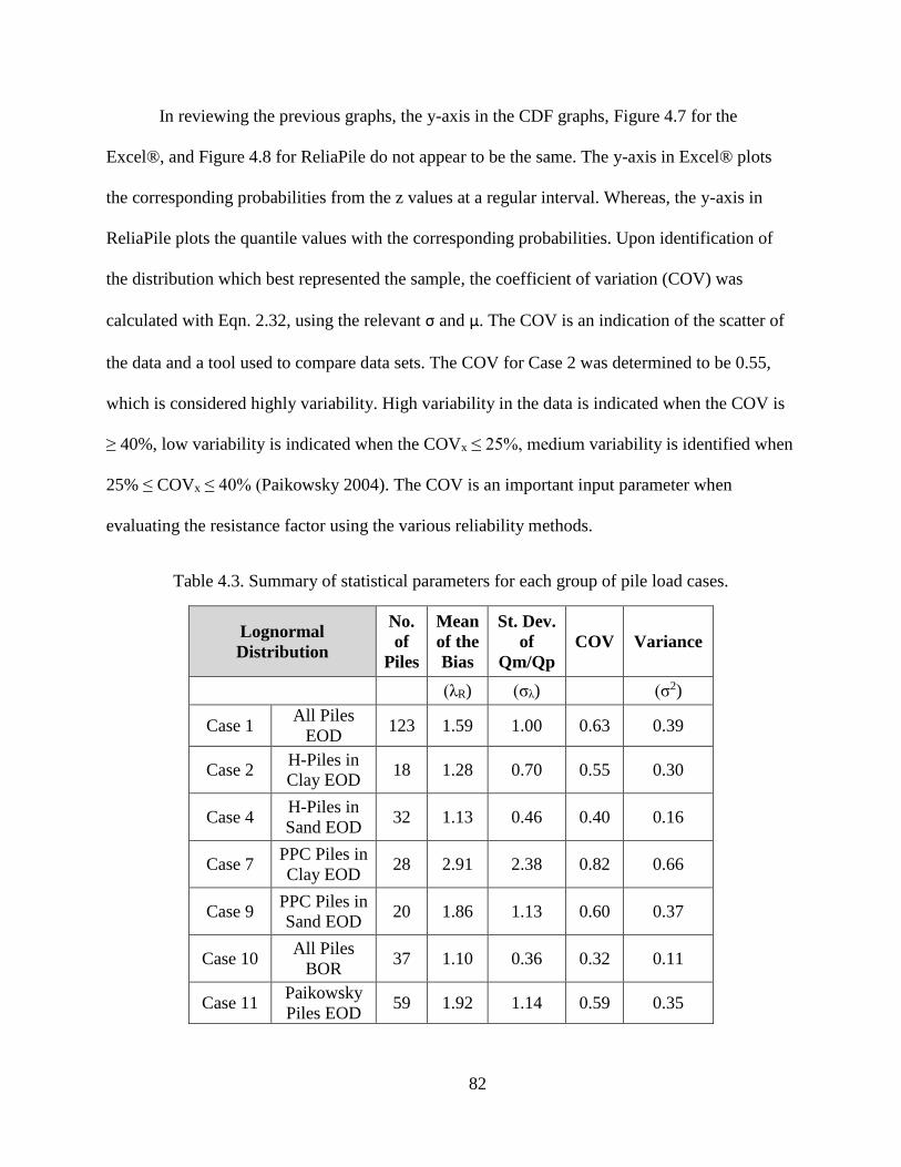
82

In reviewing the previous graphs, the y-axis in the CDF graphs, Figure 4.7 for the

Excel®, and Figure 4.8 for ReliaPile do not appear to be the same. The y-axis in Excel® plots

the corresponding probabilities from the z values at a regular interval. Whereas, the y-axis in

ReliaPile plots the quantile values with the corresponding probabilities. Upon identification of

the distribution which best represented the sample, the coefficient of variation (COV) was

calculated with Eqn. 2.32, using the relevant σ and μ. The COV is an indication of the scatter of

the data and a tool used to compare data sets. The COV for Case 2 was determined to be 0.55,

which is considered highly variability. High variability in the data is indicated when the COV is

≥ 40%, low variability is indicated when the COVx ≤ 25%, medium variability is identified when

25% ≤ COVx ≤ 40% (Paikowsky 2004). The COV is an important input parameter when

evaluating the resistance factor using the various reliability methods.

Table 4.3. Summary of statistical parameters for each group of pile load cases.

Lognormal

Distribution

No.

of

Piles

Mean

of the

Bias

St. Dev.

of

Qm/Qp

COV Variance

(λR) (σλ) (σ2)

Case 1 All Piles

EOD 123 1.59 1.00 0.63 0.39

Case 2 H-Piles in

Clay EOD 18 1.28 0.70 0.55 0.30

Case 4 H-Piles in

Sand EOD 32 1.13 0.46 0.40 0.16

Case 7 PPC Piles in

Clay EOD 28 2.91 2.38 0.82 0.66

Case 9 PPC Piles in

Sand EOD 20 1.86 1.13 0.60 0.37

Case 10 All Piles

BOR 37 1.10 0.36 0.32 0.11

Case 11 Paikowsky

Piles EOD 59 1.92 1.14 0.59 0.35

83

4.2.4 Chi-Squared Goodness-Of-Fit Test

Through visual inspection, the lognormal distribution appeared to fit the data better than

the normal distribution, but this must be verified through statistical testing by the goodness of fit

test. The Chi-Squared Test was conducted on Case 1 through Case 11 for the CDF data at 95%

confidence level to confirm which distribution (normal or lognormal) best fit the data. The

results of these analyses are presented in Table 4.4. These analyses were performed using the

arithmetic standard deviations determined from Excel® functions and confirmed with the

ReliaPile results. To perform the test, the null hypothesis that the distributions were lognormal

was evaluated and a Chi-Squared statistical value calculated. The Chi-Squared statistical values

were compared against the critical value for the upper bound of a 95% confidence level with nine

degrees of freedom. If both the normal and lognormal distributions were accepted (a value less

than the critical value), the distribution with the smaller Chi-Squared statistical value had the

stronger correlation to the data, and was the chosen distribution. Table 4.4 tabulates the

calculated Chi-Squared statistical values determined from Excel® for both distributions in each

case and the ReliaPile program check. In the Excel® calculations, the lognormal distributions

meet the null hypothesis and were the smaller of the statistical values if both the normal and

lognormal met the criteria.

84

Table 4.4. Chi-Squared Test for Cumulative Distribution Function (CDF) for Case 1 through

Case 11

Excel® ReliaPile

Crit. Value 16.92

Chi-Square Values (χ2)

Normal Lognormal Normal Lognormal

Case 1 98.49 8.00 Accept Accept

Case 2 12.00 6.44 Accept Accept

Case 4 13.63 8.63 Accept Accept

Case 7 13.43 4.14 Accept Accept

Case 9 18.00 14.00 Accept Accept

Case 10 13.13 9.22 Accept Accept

Case 11 56.42 5.58 Accept Accept

4.2.5 Confidence Bounds at 95.0% Confidence Level

The confidence interval (CI) provides an estimate of the likelihood a data point will fall

within the stated range and a measure of the goodness-of-fit of the distribution. A 95% CI means

that 95% of the time, data points will be located within this range. The CI was constructed for the

lognormal distribution as described in Section 3.4.5. These confidence bounds are illustrated in

Figure 4.9 with Excel® and Figure 4.10 with ReliaPile and demonstrated that the data points for

Case 2 did fall with the stated CI. A CI of 95% captured all of the data points for each case with

exceptions illustrated in Case 4 and Case 7, each with one data point just outside the bounds.

85

Figure 4.9. Microsoft Excel® confidence bounds for Predicted Log-Normal Distribution at

95.0% Confidence Level of steel H-Piles in clay soil (Case 2)

Figure 4.10. ReliaPile confidence bounds for Predicted Log-Normal Distribution at 95.0%

Confidence Level of steel H-Piles in clay soil (Case 2)

0.0

0.1

0.2

0.3

0.4

0.5

0.6

0.7

0.8

0.9

1.0

0.0 0.5 1.0 1.5 2.0 2.5 3.0

Cu

mu

lati

ve

Pro

ba

bil

ity

Fu

nct

ion

(C

DF

)

Qmeasured/Qpredicted

Data Points

Lognormal Dist.

Upper CI

Lower CI

86

4.3 Case 4: Steel H-Piles in Sand Soil

Case 4 represents the 32 steel H-piles driven in sandy soil. The regression analysis

presented in Figure 4.11 shows a good balance about the LOE, with the regression line having

nearly perfect agreement with the LOE at capacities less than 600 kips. An outlying data point

with a SLT capacity of 900 kips was identified as a pile from the Paikowsky 2004 report driven

in Iowa. Sufficient information was not available to ascertain why this data point was an outlier.

The PDF for steel H-piles in sand soil is represented in Figure 4.12. The observed

distribution can be considered log-normally distributed. A lognormal distribution is identified by

the CDF in Figure 4.13 and confirmed by the Chi-Squared Test results presented in Table 4.4.

The lognormal mean (μ) was 1.130 and the corresponding standard deviation (σ) was 0.456.

When a 95% confidence level was applied to the distribution all but one data point fell within the

bounds. That single data point was located just outside the CI boundary. Case 4 had a resulting

COV of 0.40 (medium variability of λ) and a variance of 0.16.

87

Figure 4.11. ReliaPile linear regression plot for steel H-Piles in sandy soil (Case 4)

Figure 4.12. ReliaPile probability density function plot (PDF) of steel H-Piles in sandy soil

(Case 4)

88

Figure 4.13. ReliaPile cumulative distribution function plot (CDF) of steel H-Piles in sandy soil

(Case 4)

Figure 4.14. ReliaPile confidence bounds for Predicted Log-Normal Distribution at 95.0%

Confidence Level of steel H-Piles in sandy soil (Case 4)

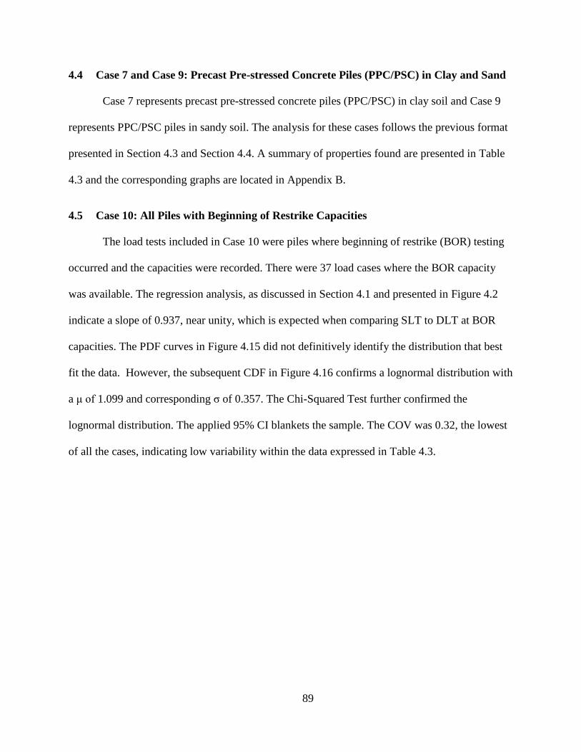
89

4.4 Case 7 and Case 9: Precast Pre-stressed Concrete Piles (PPC/PSC) in Clay and Sand

Case 7 represents precast pre-stressed concrete piles (PPC/PSC) in clay soil and Case 9

represents PPC/PSC piles in sandy soil. The analysis for these cases follows the previous format

presented in Section 4.3 and Section 4.4. A summary of properties found are presented in Table

4.3 and the corresponding graphs are located in Appendix B.

4.5 Case 10: All Piles with Beginning of Restrike Capacities

The load tests included in Case 10 were piles where beginning of restrike (BOR) testing

occurred and the capacities were recorded. There were 37 load cases where the BOR capacity

was available. The regression analysis, as discussed in Section 4.1 and presented in Figure 4.2

indicate a slope of 0.937, near unity, which is expected when comparing SLT to DLT at BOR

capacities. The PDF curves in Figure 4.15 did not definitively identify the distribution that best

fit the data. However, the subsequent CDF in Figure 4.16 confirms a lognormal distribution with

a μ of 1.099 and corresponding σ of 0.357. The Chi-Squared Test further confirmed the

lognormal distribution. The applied 95% CI blankets the sample. The COV was 0.32, the lowest

of all the cases, indicating low variability within the data expressed in Table 4.3.

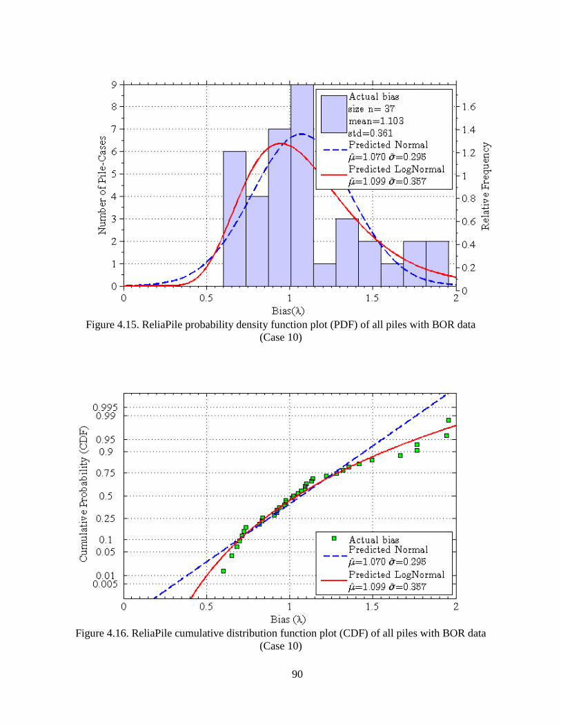
90

Figure 4.15. ReliaPile probability density function plot (PDF) of all piles with BOR data

(Case 10)

Figure 4.16. ReliaPile cumulative distribution function plot (CDF) of all piles with BOR data

(Case 10)

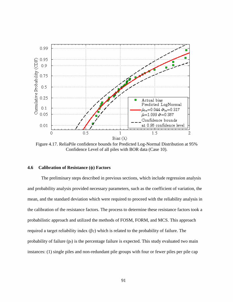
91

Figure 4.17. ReliaPile confidence bounds for Predicted Log-Normal Distribution at 95%

Confidence Level of all piles with BOR data (Case 10).

4.6 Calibration of Resistance (ϕ) Factors

The preliminary steps described in previous sections, which include regression analysis

and probability analysis provided necessary parameters, such as the coefficient of variation, the

mean, and the standard deviation which were required to proceed with the reliability analysis in

the calibration of the resistance factors. The process to determine these resistance factors took a

probabilistic approach and utilized the methods of FOSM, FORM, and MCS. This approach

required a target reliability index (βT) which is related to the probability of failure. The

probability of failure (pf) is the percentage failure is expected. This study evaluated two main

instances: (1) single piles and non-redundant pile groups with four or fewer piles per pile cap

92

with β=3.00, resulting in a pf of 0.1%, and (2) pile groups with five or more piles per pile cap

with β=2.33 resulting in a pf of 1.0% (Paikowsky et al. 2004).

As described in Chapter 3, the FOSM had two approaches: The Simplified FOSM

method utilizes a closed form solution with the assumption that the sum of the COVQ is simply

the sum of the COV for the dead load and COV of the live load (Eqn. 2.24), the second

approach, called the Improved FOSM where the COVQ in the closed form expression is

expanded as illustrated in Eqn. 2.40. The resistance factors obtained from the Improved FOSM

were higher than those found with the Simplified FOSM. This slight difference was attributed to

how the COVQ term is expressed in Eqn. 2.38 and Eqn. 2.40.

The ϕ factors obtained from FOSM Simplified method were approximately eight percent

lower than the ϕ factors obtained by all other reliability methods. The resistance factors derived

from the Improved FOSM method were in better agreement with the values obtained from the

FORM and MCS methods. Values of resistance (ϕ) factors for both β = 3.00 and β = 2.33, for

each load case are presented in Table 4.5.

The cases in this study were evaluated at both β=3.00 and β=2.33 and reported in Table

4.5. The reliability indexes that were selected for comparison are from AASHTO Table

10.5.5.2.3-1 (Table 2.3). According to AASHTO, the resistance factor recommended for a single

or non-redundant pile group using DLT with signal matching at BOR conditions is 0.50

(AASHTO 2010), and for a redundant pile group, the resistance factor is 0.65 (AASHTO 2010).

It is important to note that Cases 1, 2, 4, 7, 9, and 11 are EOD conditions, not the recommended

condition under which to determine resistance factors. These cases clearly show a lower

93

resistance factor than the AASHTO recommended value of 0.50 and 0.65 for non-redundant and

redundant pile group systems.

FO

SM

Sim

p.

FO

SM

Imp.

FO

RM

MC

S

AA

SH

TO

2010

BO

R

3.0

00.2

80.3

10.3

10.3

10.5

00.1

9

2.3

30.4

30.4

60.4

60.4

50.6

50.2

8

3.0

00.2

80.3

10.3

10.3

10.5

00.2

4

2.3

30.4

10.4

40.4

40.4

40.6

50.3

4

3.0

00.3

70.4

10.4

20.4

20.5

00.3

7

2.3

30.5

00.5

40.5

40.5

40.6

50.4

8

3.0

00.3

20.3

40.3

40.3

40.5

00.1

2

2.3

30.5

30.5

50.5

60.5

50.6

50.1

9

3.0

00.3

50.3

80.3

90.3

80.5

00.2

0

2.3

30.5

30.5

60.5

60.5

60.6

50.3

0

3.0

00.4

40.5

10.5

10.5

10.5

00.4

6

2.3

30.5

70.6

40.6

40.6

30.6

50.5

8

3.0

00.3

70.4

10.4

10.4

10.5

00.2

1

2.3

30.5

60.5

90.5

90.5

90.6

50.3

1

Lo

gno

rma

l

Dis

trib

uti

on

ϕ

No

. of

Piles

Mea

n o

f

the B

ias

(λR)

CO

V

Rel.

Index

(β)

MC

S

ϕ/λ

0.5

51.2

818

H-P

iles

in

Cla

y E

OD

Cas

e 2

0.6

31.5

9123

All

Pile

s E

OD

Cas

e 1

Cas

e 7

Cas

e 4

H-P

iles

in

San

d E

OD

32

1.1

30.4

0

1.8

60.6

0

0.8

22.9

128

PP

C P

iles

in

Cla

y E

OD

Cas

e 1

1P

aik

ow

sky

Pile

s E

OD

59

1.9

20.5

9

0.3

21.1

037

All

Pile

s B

OR

Cas

e 1

0

Cas

e 9

PP

C P

iles

in

San

d E

OD

20

Tab

le 4

.5. R

esis

tance

fac

tors

(ϕ

) fo

r ta

rget

rel

iabil

ity i

ndex

(β

T)

of

3.0

(non

-red

und

ant

pil

es)

and 2

.33

(red

undan

t pil

es)

94

However, Case 10 is relevant for AASHTO resistance factor comparison because it

contains BOR testing condition; the preferred condition to obtain resistance factors. Analyzing

piles at beginning-of-restrike (BOR) produces which is better correlated with the results of static

load testing and leads to a ratio of Qmeasured/Qpredicted, closer to unity (Table 4.5). Based on

the data collected in this study, both the non-redundant and redundant pile group systems

resistance factors of 0.51 and 0.63, respectively, show strong agreement with the AASHTO

recommended values.

Another aspect of this analysis was to determine if the soil type (clay, sand, or mixed)

and pile type affected the value of the resistance factor. In Table 4.5, of the non-redundant pile

group cases at EOD, H-Piles in sand produced the highest resistance factor of 0.42, nearest to the

AASHTO recommended. For the redundant pile group cases at EOD, PPC Piles in sand

produced the highest resistance factor of 0.56. These observations are preceded with the caveat

that these factors were determined with EOD testing and analysis, not the BOR testing and

analysis suggested. However, it suggests that a larger database of load tests taken at BOR would

possibly allow the segregation of piles by type and soil profile which could lead to higher

resistance factors.

4.7 Analysis of Piles in Paikowsky 2004 Report

The resistance factors calculated in Section 4.6 from the reliability methods were in

agreement with each other, but they should be checked against a proven baseline. The Paikowsky

et al. (2004) report presents a worldwide database, from which the current AASHTO

recommended resistance factors were determined. The Paikowsky et al. (2004) study included

338 load tests with SLT and DLT at EOD.

95

Case 11 was a subset of that database containing 59 piles that were analyzed

independently to determine the resistance factors using FOSM, FORM, and MCS. The ϕ factor

presented in Table 4.5 for β=3.00 was within 18% of the AASHTO recommended ϕ factor. For

β=2.33, the ϕ factor was within 9 % of the AASHTO recommended value presented in Table 4.5.

The agreement in resistance factors between this subset of data and the full Paikowsky database

tends to validate the process of resistance factor calibration used in this study.

4.8 Efficiency

The resistance factor alone cannot always determine which deign method or, in this

instance, which case was most efficient. The efficiency of a given resistance factor is defined in

this study to be the ration of the resistance factor over the mean value of the ratio of measured to

predicted capacity, ϕ/λ. The ϕ factors use to determine efficiency were taken from the MCS

analyses because MCS is the AASAHTO recommended method for reliability analysis. When

comparing the 11 cases, high levels of efficiency correspond to those cases where the COV

values were low. The data, presented in Table 4.5, indicates Case 10 is the most efficient of all

the cases with an efficiency of 0.46 (non-redundant piles) and 0.58 (redundant piles). This

further confirms the fact that BOR data is a better indicator of static capacity.

4.9 BOR Resistance Factors with Reliability Indexes

From the information developed in this study it is clear that evaluation of driven piles at

BOR is the preferred method to determine resistance factors. Case 10 allowed for a comparison

between the AASHTO recommended resistance factors at two reliability indexes with the values

determined using this database. The database objective was to contain load cases that were

representative of piles driven in soils similar to those found in Arkansas, to evaluate the

suitability of the AASHTO recommended resistance factors for the Arkansan environment. The

96

comparison included only the values obtained from the MCS analysis, as this is the preferred

probability analysis (Paikowsky et al. 2010). The analysis correlated with the reliability indexes

of 3.05 and 2.28 for redundant and non-redundant groups when evaluated with the AASHTO

criteria using the MCS results.

4.10 Summary

In general the ϕ factors determined in this study for EOD capacities were lower than the

AASHTO recommended values by 30% when considering only EOD capacities. However, when

considering Case 10, where the BOR capacities were used, the factors were very similar to the

AASHTO recommended values. The low resistance factors obtained for EOD capacities further

reinforces the AASHTO recommendation that EOD data should not be used for pile acceptance.

The lack of improvement in resistance factors from this study may be due to the quality of the

data reported in the literature or the limited quantity of data in some of the load cases categories

considered in this study. Some data points, that might be considered outliers, could not be fully

evaluated because the information necessary to make such a decision was not included in the

parent document. The grouping of the data may also have impacted the results; more detailed soil

information which would allow better soil classification, pile capacity development information

(end bearing versus friction piles), or more load tests for each case may have changed the way

pile load tests were grouped with a resulting positive impact on the resistance factors.

Improvements are possible with more BOR data in each pile/soil groupings.

97

5 Conclusions

Pile capacity prediction is a necessity to insure safe and economical foundations for

structures of all types. Pile capacity is most accurately measured through static load testing

(SLT) but with an associated high cost and time requirement. More economical methods, such as

dynamic load testing (DLT), are available to predict pile capacity. The comparison of capacities

measured using SLT to those derived through DLT provides a reference tool when only DLT

methods are used to determine pile capacity in the field.

Resistance factors were developed in this study that may be considered specific to the

landforms found in the State of Arkansas. These resistance factors were obtained by conducting

reliability analyses on a database of 138 load tests. The load tests were conducted at sites with

subsurface conditions similar to the conditions found within the State of Arkansas. The reliability

analyses consisted of First Order Second Moment, First Order Reliability Method, and Monte

Carlo Simulation. The following conclusions may be inferred from the data:

1. In many cases the data available in the literature for individual load tests was insufficient

to determine why a load test might be considered an outlier; this resulted in potentially

higher coefficients of variation and correspondingly lowers resistance factors.

2. Segregating piles into categories had the general effect of reducing resistance factors

rather than improving them.

3. The simplified FOSM method resulted in lower values for resistance factors and should

not be used for the calibration of resistance factors.

4. The Improved-FOSM, FORM or MCS all produce resistance factors (ϕ) that are nearly

identical and are approximately 10% higher than the resistance factors derived from the

simplified FOSM method. While the MCS is the AASHTO preferred reliability method,

98

the analyses show the Improved-FOSM produces similar resistance factors and requires

far less computing capability.

5. Capacities derived from BOR information more closely mirror the capacities measured

from static load tests with less variance than capacities derived from EOD data.

6. Resistance factors derived from this study when using cases with EOD data are

approximately 30 percent lower than those suggested by AASHTO 2010.

7. Based on the results of this study, only data from the BOR dynamic testing should be

used to ascertain pile capacity.

5.1 Future Work

With the observed results from the resistance factor determination, it is evident that

subsequent research is required to achieve more definitive results in the classification of soil and

more data is required to create statistically significant sample populations when grouping by pile

type. It is recommended that:

1. Since segregating piles into categories had the general effect of reducing resistance

factors rather than improving them. The creation of a more complete database that

includes:

a. Significantly more load cases.

b. Complete soil information, for all load test which includes strength parameters

c. Contain SLT information from load tests carried to the Davison Offset failure

criteria and contain DLT information at BOR.

d. Contain sufficient driving information to determine why a load test might be

considered an outlier.

e. Known the time lapse between driving and BOR or SLT

99

f. More complete information from signal matching to include damping factors

(quakes and side resistance) and the level of signal match quality.

2. Generate new load test data within the State of Arkansas that includes high quality soils

data and well supervised SLT and DLT information.

100

References

AASHTO. (2010). LRFD Bridge Design Specifications (5th ed.) with 2010 Interim Revisions.

Washington, D. C. American Association of State Highway and Transportation Officials.

Online: http://app.knovel.com/hotlink/toc/id:kpAASHTO11/aashto-lrfd-bridge-design-3.

Accessed June 2013.

Abu-Farsakh, M. Y., Yoon, S., and Tsai, C. (2009). Calibration of Resistance Factors Needed in

the LRFD Design of Driven Piles. No. FHWA/LA. 09/449.

AHTD. (2007). Arkansas 2003 Standard Specification for Highway Construction. Arkansas State

Highway and Transportation Department. Section 805. 731-759.

Allen, T. M. (2005). Development of the WSDOT Pile Driving Formula and its Calibration for

Load and Resistance Factor Design (LRFD). No. WA-RD 610.1.

Alvarez, C., Zuckerman, B., and Lemke, J. (2006). Dynamic Pile Analysis Using CAPWAP and

Multiple Sensors. In ASCE GEO Congress: Atlanta, Georgia. (CD-ROM).

American Petroleum Institute. (1984). Recommended Practice for Planning, Designing and

Constructing Fixed Offshore Platforms (15th ed.). Code RP 2A. Dallas, TX.

Arkansas Geological Survey (AGS). General Geology. Online: http://www.geology.ar.gov/

geology/general_geology.htm. Accessed September 2012.

ASTM Standard D1143/D1143M. (2007). Standard Test Method for Deep Foundations under

Axial Compressive Load. ASTM International. West Conshohocken, PA.

ASTM Standard D4945. (2008). Standard Test Method of High-Strain Dynamic Testing of Deep

Foundations. ASTM International, West Conshohocken, PA.

ASTM Standard D7383. (2008). Standard Test Methods for Axial Compressive Force Pulse

(Rapid) Testing of Deep Foundations. ASTM International, West Conshohocken, PA.

Baecher, G. B., and Christian, J. T. (2003). Reliability and Statistics in Geotechnical

Engineering. John Wiley & Sons Inc.

Barker, R., Duncan, J., Rojiani, K., Ooi, P., Tan, C., and Kim, S. (1991). NCHRP Report 343:

Manuals for the Design of Bridge Foundations. TRB, National Research Council,

Washington, DC.

Bradshaw, A. S., and Baxter, C. D. (2006). Design and Construction of Driven Pile Foundations-

Lessons Learned on the Central Artery/Tunnel Project. No. FHWA-HRT-05-159.

Brown, D. A., & Thompson, W. R. (2011). Developing Production Pile Driving Criteria from

Test Pile Data. NCHRP Synthesis 418. Transportation Research Board.

101

Chrimes, M. (2008). Geotechnical Publications before Geotechnique. Geotechnique, 58(5), 343-

355.

Coduto, D.P. (2001). Foundation Design: Principles and Practices (2nd ed.). Prentice Hall Inc.,

New Jersey.

Coe, D. (2009). Fisher Matrices and Confidence Ellipses: A Quick-Start Guide and Software.

Accessed June 2013.

Davisson, M. T. (1972). High Capacity Piles. In Proceedings of Soil Mechanics Lecture Series

on Innovations in Foundation Construction. American Society of Civil Engineers. Illinois

Section. Chicago, IL. 81 - 112.

DeBeer, E. E. (1968). Proefondervindlijke bijdrage tot de studie van het grensdraag vermogen

van zand onder funderingen op staal. Tijdshift der Openbar Verken van Belgie, No. 6.

Decourt, L. (1999). Behavior of Foundations under Working Load Conditions. Proceedings of

the 11th Pan-American Conference on Soil Mechanics and Geotechnical Engineering.

Foz DoIguassu, Brazil. Vol. 4. 453 - 488.

DOI. (2008). Louisiana: Reasonably Foreseeable Development Scenario for Fluid Minerals. U.S.

Department of the Interior. Bureau of Land Management Eastern States, Jackson Field

Office. Jackson, MS. Online: http://www.blm.gov. Accessed September 2012.

Fellenius, B. H. (1999). Using the Pile Driving Analyzer. Pile Driving Contractors Association,

PDCA. Annual Meeting, San Diego, CA.

Fellenius, B. H. (2001). What Capacity Value to choose from the Results of a Static Loading

Test. Paper presented at the Fulcrum, Deep Foundation Institute New Jersey.

FHWA. (1998). Driven 1.0: A Microsoft Windows™ Based Program for Determining Ultimate

Vertical Static Pile Capacity. Federal Highway Administration. Publication No. FHWA-

SA-98-074.

FHWA. (2001). Load and Resistance Factor Design (LRFD) for Highway Bridge Substructures.

Reference Manual and Participant Workbook. Federal Highway Administration. NHI

Course No. 132068. Publication No. FHWA HI-98-032.

Fragaszy, R. J., Higgins, J. D., & Lawton, E. C. (1985). Development of Guidelines for

Construction Control of Pile Driving and Estimation of Pile Capacity-Phase I-Final

Report. WA-RD 68.1, Washington State Transportation Center (TRAC).

GRL Engineers, Inc. (2014). About Dynamic Foundation Testing. Online: http://www.pile.com/

aboutdynamictesting/. Accessed May 7, 2014.

Goble, G. (2008). Driven Pile Installation and Capacity Determination. Application of Dynamic

Methods to the Design and Installation of Driven Piles. The 2007 Karl Terzaghi Lecture.

American Society of Civil Engineers.

102

Goble, G. G., and Hussein, M. H. (2000). Deep foundation capacity—What is it? Proceeding.

Performance Confirmation of Constructed Geotechnical Facilities. GSP No. 94, ASCE,

Reston, VA.

Goble, G. G., Likins, G. E., and Rausche, F. (1975). Bearing Capacity of Piles from Dynamic

Measurements. Ohio Department of Transportation. Cleveland, OH.

GRL-PDI. (2000). Deep Foundations: Believing Without Seeing. Newsletter No. 38. Goble

Rausche Likins and Associates, Inc. and Pile Dynamics, Inc. Cleveland, OH.

Hammersley, J. M., and Handscomb, D. C. (1964). Monte Carlo Methods, Methuen's

Monographs on Applied Probability and Statistics. Methuen & Co., London.

Hannigan, P. (2009). Special Design and Construction Considerations. Pile Driving Contractors

Association. Online: http://www.piledrivers.org/pdpi-lectures.htm. Accessed May 2013.

Hannigan, P.J., Goble, G.G., Likins, G.E. and Rausche, F. (2006). Design and Construction of

Driven Pile Foundations Reference Manual –Volume II. Publication No. FHWA NHI-05-

043. National Highway Institute. Federal Highway Administration.

Hannigan, P. J., Goble, G. G., Thendean, G., Likins, G. E., and Rausche, F. (1998). Design and

Construction of Driven Pile Foundations, Workshop Manual. Vol. 2. Publication No.

FHWA-HI-97-014. Federal Highway Administration. Washington, DC.

Hansen, J. B. (1963). Discussion on Hyperbolic Stress-Strain Response. Cohesive Soils.

American Society of Civil Engineers. Journal for Soil Mechanics and Foundation

Engineering. Vol. 89 (SM 4). 241 – 242.

Heiberger, R. M. and Becker, R. A. (1992). Design of an S Function for Robust Regression

Using Iteratively Reweighted Least Squares. Journal of Computational and Graphical

Statistics, American Statistical Association, Institute of Mathematical Statistics, and

Interface Foundation of America. Vol. 1. No. 3. Article DOI: 10.2307/1390715. 181-196.

Hill, J. W. (2007). Evaluation of Load Tests for Driven Piles for the Alabama Department of

Transportation. (Master’s Thesis). Auburn University, Auburn, AL.

Jabo, J. (unpublished b). ReliaPile 1.0: A MATLAB® Based Program for Analyzing Pile

Capacity Distribution and LRFD Calibration for Driven Piles. User's Manual.

Kolsky, H. (1963). Stress Waves in Solids (Vol. 1098). Dover Publication, Inc.

Kraft, L. M., Amerasinghe, S. F., and Focht, J. A. (1981). Friction Capacity of Piles Driven into

Clay. Journal of the Geotechnical Engineering Division. Vol. 107(11). 1521-1541.

Kroese, D. P., Taimre, T., & Botev, Z. I. (2011). Handbook of Monte Carlo Methods. John

Wiley & Sons, Inc. Hoboken, New Jersey

103

Kyfor, Z.G., Schnore, A.S., Carlo, T.A. and Bailey, P.F. (1992). Static Testing of Deep

Foundations. Federal Highway Administration. Report No. FHWA-SA-91-042, U.S.

Department of Transportation

Likins, G., Fellenius, B., and Holtz, R. (2012). Pile Driving Formulas: Past and Present. Full-

Scale Testing and Foundation Design. 737-753.

Loadtest USA. (2012). Telephone interview.

Long, J. H., Hendrix, J., and Jaromin, D. (2009). Comparison of Five Different Methods for

Determining Pile Bearing Capacities. No. WisDOT 0092-07-04. Wisconsin Highway

Research Program.

Long, J. H., Kerrigan, J. A., and Wysockey, M. H. (1999). Measured Time Effects for Axial

Capacity of Driven Piling. Transportation Research Record: Journal of the Transportation

Research Board. 1663(1). 8-15.

MathWorks, Inc. (2005). MATLAB: the language of technical computing. Desktop tools and

development environment, version 7. Vol. 9. MathWorks.

Maier, H. R., Lence, B. J., Tolson, B. A., and Foschi, R. O. (2001). First‐order reliability method

for estimating reliability, vulnerability, and resilience. Water Resources Research. 37(3).

779-790.

Meyerhof, G. (1976). Bearing Capacity and Settlement of Pile Foundations. Journal of the

Geotechnical Engineering Division. American Society of Civil Engineers. 102(3). 195-

228.

Middendorp, P. (2000). Statnamic: The Engineering of Art. In Proceedings of the 6th

International Conference on the Application of Stress Wave Theory to Piles. Sao Paulo,

Brazil.

Miller, I. and Freund, J. E. (1985). Probability and Statistics for Engineers. Third edition.

Englewood Cliffs, NJ: Prentice-Hall.

Neale, M. C., & Miller, M. B. (1997). The Use of Likelihood-Based Confidence Intervals in

Genetic Models. Behavior Genetics, 27(2), Kluwer Academic Publishers-Plenum

Publishers, pp. 113-120.

Nordlund, R. L. (1963). Bearing Capacity of Piles in Cohesionless Soils. American Society of

Civil Engineers. Journal of Soil Mechanics and Foundation Engineering. Vol. 89 (SM 3).

1-35.

Olson, R. E., and Flaate, K. S. (1967). Pile-Driving Formulas for Friction Piles in Sand. Journal

of Soil Mechanics and Foundation Division. ASCE, No. SM 6, 279−296.

Paikowsky, S. G. (2002). Load and Resistance Factor Design (LRFD) for Deep

Foundations. Proceedings of IWS Kamakura 2002 Foundation Design Codes and Soil

104

Investigation in view of International Harmonization and Performance. Tokyo, Japan. 59-

94

Paikowsky, S. G., Canniff, M. C., Lesny, K., Kisse, A., Amatya, S., and Muganga, R. (2010).

LRFD design and construction of shallow foundations for highway bridge structures.

NCHRP Report 651. Transportation Research Board. Washington, DC.

Paikowsky, S. G., Kuo, C., Baecher, G., Ayyub, B., Stenersen, K., .,…and O’Neill, M. (2004).

Load and Resistance Factor Design (LRFD) for Deep Foundations. NCHRP Report 507.

Transportation Research Board. Washington, DC.

Patev, R. C. (2010). Risk Technology Workshop: Engineering Reliability Concepts, Introduction

to Engineering Reliability. United States Army Corps of Engineers.

PDI. (2002). Dynamic Pile Testing with the Pile Driving Analyzer. Quality Assurance for Deep

Foundations. Pile Dynamics, Inc. Online: http://www.dot.state.oh.us/Divisions/

Engineering/ Structures/standard/Geotechnical/Documents/ODOT. Accessed October

2012.

PDI. (2012). Pile Dynamics, Inc. Telephone interview.

Phoon, K. K., Kulhawy, F. H., & Grigoriu, M. D. (2003). Development of a reliability-based

design framework for transmission line structure foundations. Journal of Geotechnical

and Geoenvironmental Engineering. 129(9). 798-806.

Raychaudhuri, S. (2008). Introduction to Monte Carlo Simulation. In Simulation Conference,

2008. WSC 2008. IEEE. 91-100.

Reese, L. C., Isenhower, W. M., Wang, and Shin-Tower (2006). Analysis and Design of Shallow

and Deep Foundations. John Wiley & Sons, Inc. Hoboken, New Jersey.

Rubinstein, R. Y. (1981). Simulation and the Monte Carlo Method. John Wiley & Sons, Inc.

New York.

Smith, E. A. (1962). Pile-Driving Analysis by the Wave Equation. American Society of Civil

Engineers Transactions. Vol. 27. 1145–1193.

Statnamic Load Testing Overview. Applied Foundation Testing. Inc. Online:

http://www.testpile.com/PDF/Statnamic%20Testing%20Brief%20Overview%20for%20

Web%20Site.pdf. Accessed August 2012.

Steele, R., Seidel, J., and Klingberg, D., (1990). Test Piling Program for Bridges on the Sunshine

Motorway in Queensland. Australian Road Research Board (ARRB) Conference. 15th.

Darwin, Northern Territory. 139-153.

Terzaghi, K., Peck, R. B., and Casagrande, A. (1942). Discussion of Pile Driving Formulas:

Progress Report of the Committee on the Bearing Value of Pile Foundation. Proceedings

of the American Society of Civil Engineers. Vol. 68. 311-323.

105

Thendean, G., Rausche, F., Svinkin, M., Likins, G. E. (1996). Wave Equation Correlation

Studies. Proceedings of the Fifth International Conference on the Application of Stress-

wave Theory to Piles 1996. Orlando, FL. 144-162.

Tomlinson, M. J. (1957). The Adhesion of Piles Driven in Clay Soils. In Proceedings of the 4th

International Conference on Soil Mechanics and Foundation Engineering. London,

England.

Ulitskii, V. M. (1995). History of Pile Foundation Engineering. Soil Mechanics and Foundation

Engineering. 32(3). 110-114.

Valsamosa, G., Casadeia, F., Solomos, G. (2013). A Numerical Study of Wave Dispersion

Curves in Cylindrical Rods with Circular Cross-Section. Applied and Computational

Mechanics. Vol. 7. 99–114.

Vijayvergiya, V. N. and Focht, J. A. (1972). A New Way to Predict the Capacity of Piles in Clay.

Proceeding: 4th Offshore Technology Conference. Houston, TX. Vol. 2. 865-874.

Walton, P. A., and Borg, S. L. (1998). Using Dynamic Pile Testing To Evaluate Quality and

Verify Capacity of Driven Piles. Transportation Research Record. Journal of the

Transportation Research Board. Vol. 1633(1). 117-119.

Woo, C. (2013). Fisher Information Matrix. http://planetmath.org/sites/default/files/texpdf

/36041.pdf. Accessed June 20, 2014.

Yoon, S., Tsai, C., and Melton, J. M. (2011). Pile Load Test and Implementation of

Specifications of Load and Resistance Factor Design. Transportation Research Record.

Journal of the Transportation Research Board. 2212(1), 23-33.

106

Appendix A – Load Test Database

Table A.1. Load test database

Pile

No. Location Paper/Project Pile Type

Soil

Type

SLT

(kips)

DLT -

EOD

(kips)

DLT-BOR

w/PDA

(kips)

1 Alabama ALDOT-2007 HP 10x42 clay 240 240

2 Alabama ALDOT-2007 HP 10x42 clay 174 222

3 Alabama ALDOT-2007 HP 10x42 Mixed 120 180

4 Alabama ALDOT-2007 HP 10x42 sand 252 232

5 Alabama ALDOT-2007 HP 10x42 sand 240 195 220

6 Alabama ALDOT-2007 HP 12x53 clay 360 300 318

7 Alabama ALDOT-2007 HP 12x53 clay 366 210 512.8

8 Alabama ALDOT-2007 HP 12x53 Mixed 180 358 275.4

9 Alabama ALDOT-2007 HP 12x53 Mixed 180 220 264

10 Alabama ALDOT-2007 HP 12x53 MIxed 192 240 98.2

11 Alabama ALDOT-2007 HP 12x53 Mixed 198 176 149.8

12 Alabama ALDOT-2007 HP 12x53 sand 180 154

13 Alabama ALDOT-2007 HP 12x53 sand 270 176 276

14 Alabama ALDOT-2007 HP 12x53 sand 270 228

15 Alabama ALDOT-2007 HP 12x53 sand 180 178

16 Alabama ALDOT-2007 HP 12x53 sand 180 200 214.8

17 Alabama ALDOT-2007 HP 12x53 sand 180 209 300

18 Alabama ALDOT-2007 HP 12x53 sand 180 119 216

19 Alabama ALDOT-2007 HP 12x53 sand 420 419 327.4

20 Alabama ALDOT-2007 HP 12x53 sand 198 240 132.4

21 Alabama ALDOT-2007 HP 12x84 clay 180 122.6

22 Alabama ALDOT-2007 HP 14x73 clay 378 290 410

23 Alabama ALDOT-2007 HP 14x73 clay 380 370

24 Alabama ALDOT-2007 HP 14x73 Mixed 324 268 346

25 Alabama ALDOT-2007 HP 14x73 sand 342 282 241.4

26 Alabama ALDOT-2007 HP 14x89 Mixed 342 256

27 Alabama ALDOT-2007 HP 14x89 sand 270 280 366

28 Alabama ALDOT-2007 HP 14x89 sand 342 300 193.8

29 Alabama ALDOT-2007 PSC 14"

Square sand 300 360

30 Alabama ALDOT-2007 PSC 24"

Square sand 690 998 657

107

Table A.1 Cont.

Pile

No.

(Cont.)

Location

(Cont.)

Paper/Project

(Cont.)

Pile Type

(Cont.)

Soil

Type

(Cont.)

SLT

(kips)

(Cont.)

DLT -

EOD

(kips)

(Cont.)

DLT-BOR

w/PDA

(kips)

(Cont.)

31 Alabama ALDOT-2007 PSC 24"

Square sand 690 820 707.2

32 MA C/A Tunnel

Project PIPE clay 807 626 595

33 MA C/A Tunnel

Project PIPE clay 646 575 604

34 MA C/A Tunnel

Project PIPE sand 486 372 445

35 MA C/A Tunnel

Project PIPE sand 544 408 562

36 MA C/A Tunnel

Project PPC 31 cm clay 340 374 415

37 MA C/A Tunnel

Project PPC 31 cm clay 228 261 327

38 MA C/A Tunnel

Project PPC 41 cm clay 702 730

39 MA C/A Tunnel

Project PPC 41 cm clay 800 836

40 MA C/A Tunnel

Project PPC 41 cm clay 775 950 1070

41 MA C/A Tunnel

Project PPC 41 cm clay 775 578 758

42 MA C/A Tunnel

Project PPC 41 cm clay 850 370 510

43 MA C/A Tunnel

Project PPC 41 cm clay 698 604 634

44 MA C/A Tunnel

Project PPC 41 cm clay 812 453 418

45 MA C/A Tunnel

Project PPC 41 cm clay 800 344 453

46 MA C/A Tunnel

Project PPC 41 cm sand 570 537 628

47 Louisiana LADOTD-

2009

PPC 14"

Square clay 230 226.8

48 Louisiana LADOTD-

2009

PPC 14"

Square clay 344 300.2

49 Louisiana LADOTD-

2009

PPC 14"

Square clay 330 133

108

Table A.1. Cont.

Pile

No.

(Cont.)

Location

(Cont.)

Paper/Project

(Cont.)

Pile Type

(Cont.)

Soil

Type

(Cont.)

SLT

(kips)

(Cont.)

DLT -

EOD

(kips)

(Cont.)

DLT-BOR

w/PDA

(kips)

(Cont.)

50 Louisiana LADOTD-

2009

PPC 16"

Square clay 200 192

51 Louisiana LADOTD-

2009

PPC 24"

Square clay 544 150 477.6

52 Louisiana LADOTD-

2009

PPC 24"

Square clay 298 300

53 Louisiana LADOTD-

2009

PPC 24"

Square sand 154 35

54 Louisiana LADOTD-

2009

PPC 24"

Square sand 240 120

55 Louisiana LADOTD-

2009

PPC 30"

Square clay 956 273 1034.2

56 Louisiana LADOTD-

2009

PPC 30"

Square clay 928 365 759.2

57 Louisiana LADOTD-

2009

PPC 30"

Square clay 760 247 749.2

58 Louisiana LADOTD-

2009

PPC 30"

Square clay 910 325

59 Louisiana LADOTD-

2009

PPC 30"

Square sand 780 240

60 MO MODOT PIPE clay 233 550

61 H.Kong Paikowsky-

2004 HP 10x120 mixed 1055 978

62 NE Paikowsky-

2004 HP 10x42 clay 300 230

63 PA Paikowsky-

2004 HP 10x42 sand 397 398

64 PA Paikowsky-

2004 HP 10x57 sand 330 446

65 PA Paikowsky-

2004 HP 10x57 sand 300 428

66 PA Paikowsky-

2004 HP 10x57 sand 390 524

67 CAN Paikowsky-

2004 HP 10X74 mixed 350 432

68 H.Kong Paikowsky-

2004 HP 12x120 mixed 1011 1091

69 HOL Paikowsky-

2004 HP 12x120 mixed 223 156

109

Table A.1. Cont.

Pile

No.

(Cont.)

Location

(Cont.)

Paper/Project

(Cont.)

Pile Type

(Cont.)

Soil

Type

(Cont.)

SLT

(kips)

(Cont.)

DLT -

EOD

(kips)

(Cont.)

DLT-BOR

w/PDA

(kips)

(Cont.)

70 CAN Paikowsky-

2004 HP 12X53 sand 475 484

71 MA Paikowsky-

2004 HP 12x74 clay 416 304

72 MA Paikowsky-

2004 HP 12x74 clay 448 315

73 CAN Paikowsky-

2004 HP 12x74 mixed 800 439

74 CAN Paikowsky-

2004 HP 12x74 sand 570 575

75 PA Paikowsky-

2004 HP 12x74 sand 550 457

76 PA Paikowsky-

2004 HP 12x74 sand 570 512

77 PA Paikowsky-

2004 HP 12x74 sand 310 405

78 PA Paikowsky-

2004 HP 12x74 sand 272 455

79 PA Paikowsky-

2004 HP 12x74 sand 500 561

80 OK Paikowsky-

2004 HP 14x117 mixed 820 566

81 AZ Paikowsky-

2004 HP 14x117 mixed 1239 554

82 MN Paikowsky-

2004 HP 14x73 clay 740 342

83 S.C. Paikowsky-

2004 HP 14x73 sand 318 215

84 VT Paikowsky-

2004 HP 14x73 sand 315 194

85 VT Paikowsky-

2004 HP 14x73 sand 313 159

86 IA Paikowsky-

2004 HP 14x89 sand 930 367

87 NY Paikowsky-

2004 HP 10x24 sand 313 132

88 WI Paikowsky-

2004 HP 12x63 clay 315 110

89 WI Paikowsky-

2004 HP 12x63 clay 214 105

110

Table A.1. Cont.

Pile

No.

(Cont.)

Location

(Cont.)

Paper/Project

(Cont.)

Pile Type

(Cont.)

Soil

Type

(Cont.)

SLT

(kips)

(Cont.)

DLT -

EOD

(kips)

(Cont.)

DLT-BOR

w/PDA

(kips)

(Cont.)

90 NE Paikowsky-

2004 PSC 12" sq clay 354 226

91 CAN Paikowsky-

2004 PSC 12" sq mixed 500 400

92 NY Paikowsky-

2004

PSC 14"

cyl sand 324 279

93 Florida Paikowsky-

2004 PSC 14" sq clay 760 255

94 NE Paikowsky-

2004 PSC 14" sq clay 374 179

95 MA Paikowsky-

2004 PSC 14" sq clay 319 82

96 KY Paikowsky-

2004 PSC 14" sq clay 465 288

97 AZ Paikowsky-

2004 PSC 16" sq mixed 1123 529

98 S.C. Paikowsky-

2004 PSC 16" sq sand 819 170

99 Florida Paikowsky-

2004 PSC 18" sq clay 308 224

100 AL Paikowsky-

2004 PSC 18" sq sand 345 205

101 AL Paikowsky-

2004 PSC 18" sq sand 535 428

102 Florida Paikowsky-

2004 PSC 18" sq sand 265 245

103 H.Kong Paikowsky-

2004

PSC 19.69"

cyl mixed 1000 755

104 H.Kong Paikowsky-

2004

PSC 19.69"

cyl mixed 1021 1091

105 HOL Paikowsky-

2004

PSC 19.69"

cyl sand 124 147

106 OR Paikowsky-

2004 PSC 20" sq mixed 1380 559

107 OK Paikowsky-

2004

PSC 24"

oct sand 750 530

108 Louisiana Paikowsky-

2004 PSC 24" sq clay 400 136

111

Table A.1. Cont.

Pile

No.

(Cont.)

Location

(Cont.)

Paper/Project

(Cont.)

Pile Type

(Cont.)

Soil

Type

(Cont.)

SLT

(kips)

(Cont.)

DLT -

EOD

(kips)

(Cont.)

DLT-BOR

w/PDA

(kips)

(Cont.)

109 LA Paikowsky-

2004 PSC 24" sq clay 398 60

110 VA Paikowsky-

2004 PSC 24" sq mixed 1230 626

111 Florida Paikowsky-

2004 PSC 24" sq sand 965 488

112 AL Paikowsky-

2004 PSC 24" sq sand 614 340

113 AL Paikowsky-

2004 PSC 24" sq sand 773 446

114 Florida Paikowsky-

2004 PSC 24" sq sand 610 509

115 Florida Paikowsky-

2004 PSC 24" sq sand 495 450

116 Florida Paikowsky-

2004 PSC 30" sq clay 1797 1301

117 LA Paikowsky-

2004 PSC 30" sq clay 453 45

118 LA Paikowsky-

2004 PSC 30" sq clay 420 59

119 Florida Paikowsky-

2004 PSC 30" sq clay 1209 1025

120 LA Paikowsky-

2004

PSC 36"

cyl clay 471 91

121 LA Paikowsky-

2004

PSC 36"

cyl clay 488 103

122 AL Paikowsky-

2004 PSC 36" sq sand 1074 662

123 NY Paikowsky-

2004

PSC 54"

cyl sand 1452 405

124 WI Paikowsky-

2004

PSC 9.7"

sq clay 214 335

125 HOL Paikowsky-

2004

PSC 9.7"

sq sand 228 296

126 NY Paikowsky-

2004

PSC 9.7"

sq sand 480 489

127 IA PILOT HP 10x42 Clay 124 216

128 IA PILOT HP 10x42 Clay 150 244

129 IA PILOT HP 10x42 Clay 154 286

112

Table A.1. Cont.

Pile

No.

(Cont.)

Location

(Cont.)

Paper/Project

(Cont.)

Pile Type

(Cont.)

Soil

Type

(Cont.)

SLT

(kips)

(Cont.)

DLT -

EOD

(kips)

(Cont.)

DLT-BOR

w/PDA

(kips)

(Cont.)

130 IA PILOT HP 10x42 Clay 242 390

131 IA PILOT HP 10x42 Clay 212 292

132 IA PILOT HP 10x42 Mixed 52

133 IA PILOT HP 10x42 Mixed 162 328

134 IA PILOT HP 10x42 Sand 182 452

135 IA PILOT HP 10x42 Sand 128 324

136 IA PILOT HP 10x57 Mixed 198 282

137 AZ PILOT PSC 18.05"

sq sand 975

138 AZ PILOT PSC 18.05"

sq sand 1115

113

Appendix B – ReliaPile Graphs for Cases 7 and 9

Appendix B contain the ReliaPile graphs for Case 7 and Case 9 discussed in Chapter 4.

The included graphs are a linear regression plot, probability density function plot (PDF),

cumulative distribution function plot (CDF), and CDF with confidence bounds for the predicted

lognormal distribution at a 95.0% confidence level.

Figure B.1. ReliaPile Linear Regression Plot for PPC piles in clay soil (Case 7)

114

Figure B.2. ReliaPile Probability Density Function Plot (PDF) for PPC piles in clay soil

(Case 7)

Figure B.3. ReliaPile Cumulative Distribution Function Plot (CDF) for PPC piles in clay soil

(Case 7)

115

Figure B.4. ReliaPile Confidence Bounds for Predicted Log-Normal Distribution at 95.0%

Confidence Level for PPC piles in clay soil (Case 7)

Figure B.5. ReliaPile Linear Regression Plot for PPC piles in sand soil (Case 9)

116

Figure B.6. ReliaPile Probability Density Function Plot (PDF) for PPC piles in sand soil (Case 9)

Figure B.7. ReliaPile Cumulative Distribution Function Plot (CDF) for PPC piles in sand soil

(Case 9)

117

Figure B.8. ReliaPile Confidence Bounds for Predicted Log-Normal Distribution at 95.0%

Confidence Level for PPC piles in sand soil (Case 9)