CALIBRATION OF MEPDG PERFORMANCE MODELS FOR FLEXIBLE ...
103
CALIBRATION OF MEPDG PERFORMANCE MODELS FOR FLEXIBLE PAVEMENT DISTRESSES TO LOCAL CONDITIONS OF ONTARIO by NELSON FERNANDO CUNHA COELHO Presented to the Faculty of the Graduate School of The University of Texas at Arlington in Partial Fulfillment of the Requirements for the Degree of MASTER OF CIVIL ENGINEERING THE UNIVERSITY OF TEXAS AT ARLINGTON July 2016
Transcript of CALIBRATION OF MEPDG PERFORMANCE MODELS FOR FLEXIBLE ...

CALIBRATION OF MEPDG PERFORMANCE MODELS FOR FLEXIBLE PAVEMENT
DISTRESSES TO LOCAL CONDITIONS OF ONTARIO
by
NELSON FERNANDO CUNHA COELHO
Presented to the Faculty of the Graduate School of
The University of Texas at Arlington in Partial Fulfillment
of the Requirements
for the Degree of
MASTER OF CIVIL ENGINEERING
THE UNIVERSITY OF TEXAS AT ARLINGTON
July 2016

ii
Copyright © by Nelson Fernando Cunha Coelho 2016
All Rights Reserved

iii
Acknowledgements
I would like to endorse my sincere gratitude to my Supervisor, Dr. Stefan Romanoschi,
for his interest and enthusiasm in the topic, continued guidance and help to overcome barriers.
His subjects and methods motivated and attracted me to this domain of civil engineering.
I would like to express my gratitude to the members of my committee, Dr. James Williams
and Dr. Stephen Mattingly for their valuable time to review my thesis and contributions of great
value. I would like to extend my appreciation to Dr. Sia Ardekani and Dr. Victoria Chen for their
subjects and teaching.
I would like to thank Fouad Tannous and Warren Lee from the Ministry of Transportation
Ontario (MTO) for their contribution in obtaining pavement structure data and pavement
performance information.
At last, I would like to express my gratitude to my fiancé for her unceasing
encouragement and support. One final acknowledgement goes to my parents and sisters for their
education and care.
July 18, 2016

iv
Abstract
CALIBRATION OF MEPDG PERFORMANCE MODELS FOR FLEXIBLE PAVEMENT
DISTRESSES TO LOCAL CONDITIONS OF ONTARIO
Nelson Fernando Cunha Coelho
The University of Texas at Arlington, 2016
Supervising Professor: Stefan A. Romanoschi
The implementation of the American Association of State Highway and Transportation
Officials (AASHTO) Mechanistical-Empirical Pavement Design requires the development of a
design procedure that can be used by the agencies and engineering consultants to design new
and reconstructed rigid and flexible pavements. To calibrate the design procedure for a region, a
large dataset representing the particular local conditions is needed. It includes traffic, climate, site
material characteristics, performance requirements and historical data. The performance models
were calibrated in North America using the Long Term Pavement Database Program (LTPP),
therefore, the models must be calibrated to local conditions in order to obtain more suitable
parameters, formulas and predictions. It is expected that calibrated performance models using
site-specific data will predict pavement performance approximated to the performance measured
in the field. Gathering data related with observed distresses is essential for subsequent
comparison with predicted distresses.
The primary objective of this project is to calibrate the performance models of flexible
pavement distresses, including total rutting (permanent deformation) and asphalt concrete (AC)
bottom-up fatigue cracking, to the local conditions of new flexible pavement in Ontario, Canada.
Sixteen (16) representative pavement sections from widening and reconfiguration highway
projects were selected. Performance data, traffic data, structure information, materials properties

v
and performance data were obtained from site-specific investigation and pavement design reports
provided by the Ministry of Transportation Ontario (MTO).
The AASHTOWare Pavement ME DesignTM
was used to run the initial predictions using
the global calibration coefficients. Then, the obtained predicted distresses were compared with
the measured distresses to assess for local bias and goodness of fit. The analysis showed that,
using the global calibration coefficients, the AASHTOWare model under predicted alligator
cracking and over predicted total rutting. Statistical analysis, such as, Regression Analysis and
the Microsoft Solver numerical optimization routine were used to find the regression coefficients,
using the approach of minimizing the sum of squared error (SSE).
Concerning alligator cracking, the local calibration factors have improved the bias and
standard error of the estimate (SEE). Plots also showed that points are randomly scattered along
equality line and predicted values closer to the measured values.
Regarding permanent deformation (rutting), the local calibration factors have improved
the bias and standard error of the estimate. The accuracy of the transfer function has increased in
comparison to the use of the global calibration values, suggesting that the local calibration
procedure has improved the rutting model. Analyzing the plots measured versus predicted, points
are better scattered and a shift is clearly noted in the chart from global to local calibration,
indicating that local calibration coefficients improved distress estimations.

vi
Table of Contents
Acknowledgements ......................................................................................................................... iii
Abstract ............................................................................................................................................ iv
Table of Contents ............................................................................................................................ vi
List of Figures .................................................................................................................................. ix
List of Tables .................................................................................................................................... x
1 Introduction ............................................................................................................................ 1
1.1 Importance of Research ............................................................................................... 4
1.2 Research Objectives ..................................................................................................... 6
1.3 Methodology .................................................................................................................. 6
1.4 Thesis Structure ............................................................................................................ 6
2 Literature Review ................................................................................................................... 8
2.1 Pavement Design Methods Background .................................................................... 8
2.2 Ontario’s State of Practice ......................................................................................... 10
2.3 MEPDG Method ........................................................................................................... 11
2.3.1 Hierarchical Design Input Levels ............................................................................. 15
2.3.2 Pavement Performance Models for Flexible Pavements ......................................... 16
2.3.3 Design Criteria and Reliability Level ........................................................................ 17
2.4 Performance Prediction Models for Flexible Pavement .......................................... 18
2.4.1 Bottom-Up Fatigue or Alligator Cracking Model ...................................................... 18
2.4.2 Top-Down or Longitudinal Cracking Model.............................................................. 21
2.4.3 Transverse Thermal Cracking Model ....................................................................... 21
2.4.4 Permanent Deformation (Rutting) Model ................................................................. 23
2.4.4.1 Asphalt Concrete Model .................................................................................. 24
2.4.4.2 Unbound Materials .......................................................................................... 25
2.4.5 International Roughness Index (IRI) Model ............................................................. 26
3 Database Assembly ............................................................................................................. 29

vii
3.1 Local Calibration and Validation Plan ....................................................................... 29
3.2 Selection of Hierarchical Input Level ........................................................................ 29
3.3 Performance Criteria Thresholds .............................................................................. 33
3.4 Sample Size Computation .......................................................................................... 34
3.5 Selection of Pavement Segments ............................................................................. 36
3.6 Extract and Evaluate Distress and Project Data ...................................................... 38
3.6.1 Extraction, Assembly and Conversion of Measured Data ....................................... 38
3.6.2 Evaluation of Assembled Data ................................................................................. 39
3.7 Conduct Field and Forensic Investigations ............................................................. 43
3.8 Data Inputs for Design ................................................................................................ 43
3.8.1 Design Inputs ........................................................................................................... 43
3.8.2 Traffic Data .............................................................................................................. 44
3.8.3 Structural Layers and Materials Properties ............................................................. 50
3.8.3.1 HMA ................................................................................................................ 50
3.8.3.2 Unbounded Material Properties ...................................................................... 52
3.8.3.3 Subgrade Soil Type and Properties ................................................................ 52
3.8.4 Climate Data ............................................................................................................ 52
3.8.5 Pavement Performance Data .................................................................................. 53
4 Development of Calibration Models ................................................................................... 54
4.1 Assess Local Bias from Global Calibration Parameters ......................................... 55
4.1.1 Assess Local Bias for Alligator Cracking Model ...................................................... 55
4.1.2 Assess Local Bias for Rutting Model ....................................................................... 56
4.2 Eliminate Local Bias of Distress Prediction Models ............................................... 57
4.2.1 Eliminate Local Bias for Alligator Cracking Model ................................................... 59
4.2.2 Eliminate Local Bias for Rutting Models .................................................................. 63
4.3 Assess the Goodness of Fit ....................................................................................... 70
5 Summary, Conclusions and Recommendations .............................................................. 71

viii
5.1 Summary ...................................................................................................................... 71
5.2 Conclusions ................................................................................................................. 71
5.3 Recommendations ...................................................................................................... 73
Appendix A Traffic Data .................................................................................................................. 74
Appendix B Pavement Structure Information ................................................................................. 79
Appendix C Pavement Performance Data ..................................................................................... 83
Appendix D Predicted Distresses from AASHTOWare and Calculations ...................................... 85
References ..................................................................................................................................... 90
Biographical Information ................................................................................................................. 93

ix
List of Figures
Figure 1-1 Alligator Cracking (Asphalt Institute, 2016) .................................................................... 5
Figure 1-2 Rutting (Asphalt Institute, 2016) ..................................................................................... 5
Figure 2-1: Conceptual Flow Chart of the Three-Stage Design/Analysis Process for the MEPDG
(AASHTO, 2008)............................................................................................................................ 14
Figure 2-2 Rutting (FHWA, 2015) .................................................................................................. 28
Figure 3-1. Map showing Pavement Sections Selected along Central Region of Ontario ............ 37
Figure 3-2 Bottom-Up or Alligator Cracking (FHWA, 2015) .......................................................... 39
Figure 3-3. Plot showing Total Alligator Cracking (%) over time ................................................... 41
Figure 3-4. Plot showing Total Rutting (mm) over time ................................................................. 42
Figure 3-5: Example of Traffic Data Available in iCorridor ............................................................ 48
Figure 3-6: FHWA Vehicle Category Classification (FHWA, 2014) ............................................... 49
Figure 4-1: Measured vs Predicted Alligator Cracking Using Global Calibration Parameters ...... 56
Figure 4-2: Measured vs Predicted Total Rutting Using Global Calibration Parameters .............. 57
Figure 4-3: Measured vs Predicted Alligator Cracking Using Local Calibration Parameters ........ 62
Figure 4-4: Residual Error versus Predicted Alligator Cracking .................................................... 62
Figure 4-5: Measured vs Predicted AC Rutting Using Global Calibration Parameters ................. 65
Figure 4-6: Measured vs Predicted AC Rutting Using Local Calibration Parameters ................... 65
Figure 4-7: Measured vs Predicted Base Rutting Using Global Calibration Parameters .............. 66
Figure 4-8: Measured vs Predicted Base Rutting Using Local Calibration Parameters ................ 66
Figure 4-9: Measured vs Predicted Subgrade Rutting Using Global Calibration Parameters ...... 67
Figure 4-10: Measured vs Predicted Subgrade Rutting Using Local Calibration Parameters ...... 67
Figure 4-11: Measured vs Predicted Total Rutting Using Local Calibration Parameters .............. 68
Figure 4-12: Predicted Total Rutting versus Residual Error .......................................................... 68

x
List of Tables
Table 3-1 - Input Level for Traffic Parameters ............................................................................... 30
Table 3-2 - Input Level for Asphalt Concrete Material Properties Parameters ............................. 31
Table 3-3 - Input Level for Climate Parameters ............................................................................ 32
Table 3-4 - Input Level for Unbound Granular Material Properties Parameters ........................... 32
Table 3-5 - Input Level for Subgrade Material Properties Parameters .......................................... 33
Table 3-6 – Design Criteria Values................................................................................................ 34
Table 3-7 – Minimum Number of Segments Needed for Local Calibration and Validation ........... 35
Table 3-8 – List of Pavement Sections Selected ........................................................................... 37
Table 3-9 – Comparison of Units of Measured and Predicted Distresses .................................... 38
Table 3-10 – Extracted Measured Data and Pavement Age for Alligator Cracking ...................... 40
Table 3-11 – Summary of Statistic Information for Alligator Cracking and Rutting ....................... 40
Table 3-12 - Input Level for Traffic Parameters ............................................................................. 45
Table 3-13 – Percentage of Trucks in Design Lane (Ontario 2012) .............................................. 47
Table 3-14 - Input Level for Asphalt Concrete material-related variables ..................................... 51
Table 4-1 – Criteria for Determining Global Models Adequacy ..................................................... 54
Table 4-2 – Summary of Statistic Parameters – Global Calibration .............................................. 55
Table 4-3 – Potential Cause of Bias and Corrective Action (CDOT, 2013) .................................. 58
Table 4-4 – Computation of the Calibration Coefficients C1 and C2 ............................................ 60
Table 4-5 – Summary of Statistic Parameters – Local Calibration ................................................ 63
Table 4-6 –Local Calibration Coefficients ...................................................................................... 64
Table 4-7 – Summary of Statistic Parameters – Local Calibration ................................................ 69
Table 4-8 – MEPDG Statistic Parameters – Global and Local Calibration ................................... 70

1
1 Introduction
The design of a pavement structure encompasses multiple modeling steps and the
combination of many variables. Traffic load is a heterogeneous conjunction of vehicles, axle types
and configurations that fluctuate throughout the day, season and life of the pavement structure.
The pavement materials perform differently and the performance is influenced by temperature,
moisture, magnitude, stress and other factors. More complications are added when they are
exposed to severe environmental conditions including temperature differentials ranging from
torrid heat to freezing and from dry to saturated moisture states.
Numerous developments over the last decades have provided and improved the
accuracy and rationality of pavement design methods. The American Association of State
Highway Officials (AASHO), financed by State highway agencies, the U.S. Bureau of Public
Roads and other agencies and countries, constructed in 1958 a test site, called the AASHO Road
Test, to study the pavement performance under specific conditions (uniform mixtures, on a single
type of subgrade soil and under specific environmental conditions – Central Illinois). The
information obtained was used to develop an empirical method, the AASHTO Pavement Design
Guide (1972), to design flexible and rigid pavement structures. Over the years, refined versions
have been published, (1986, 1993, 1998) which improve the original empirical equations to
address shortcomings in the design procedure. The 1993 AASHTO Pavement Design Guide was
broadly adopted by states, countries and transportation agencies.
Over the latest decades, pavement design methods advanced from empirical procedures
(based on pavement performance observation) to mechanistic-empirical procedures
(incorporating pavement response, damage accumulation and distresses). This evolution is due
to advanced computational mechanics and computers that allow performing calculations, which
significantly improved the predictions of pavement responses to load and climate effects.
Improved characterization of traffic and materials, study and comprehension of climate effects on
materials, greater knowledge of pavement performance and large databases are also outcomes
of this evolution.

2
AASHTO has released the Mechanistic-Empirical Pavement Design Guide (MEPDG) –
Manual of Practice in 2008. It provides a methodology to design pavements based on
engineering models calibrated at the national level using a large amount of pavement
performance information from the LTPP database. In 2011, AASHTO lunched the associated
software AASHTOWare Pavement ME DesignTM, which is a software tool that develops and
optimizes the models of the computational project carried out as part of National Cooperative
Highway Research Program (NCHRP) Project 1-37A.
The current AASHTO Pavement Mechanistic-Empirical Design is based on the
Mechanistic-Empirical Pavement Design Guide (MEPDG) developed by the NCHRP, which works
with the fundamental properties of the pavement, base and subgrade materials. The design and
analysis procedure estimates pavement responses (stresses, strains, and deflections) and
applies those responses to calculate incremental damage. In this procedure, the cumulative
damage is empirically related to observed pavement distresses (AASHTO, 2008). In pavement
design, the Mechanistic-Empirical approach integrates two principles. Firstly, the “mechanistic”
approach is focused on the study of physical causes (loads and material properties of the
pavement structure) seeking to explain the stresses, strains and deflections. The correlations
between physical causes and phenomena are depicted using mathematical models, being the
most common the layered elastic model. Secondly, the “empirical” approach deals with the
observed performance to determine relationships. The estimated responses (stresses, strains
and deflections) of a selected pavement segment will be tied with the observed performance
International Roughness Index (IRI) and surface distresses (permanent deformation and
cracking) under diverse traffic loading and climatic conditions in order to define what values result
in pavement failure. Correlations between pavement failure and physical phenomena are
represented by derived equations that calculate the number of loading cycles to failure.

3
The MEPDG design procedure is an iterative process. The procedure does not provide
thickness. Instead, the outputs from the procedure are pavement distresses and smoothness.
Site conditions, namely, traffic, material and subgrade properties, climate and pavement condition
are considered for a trial design for a new pavement or rehabilitation project. The adequacy of the
trial design is then assessed when compared with performance criteria and reliability through the
prediction of pavement distresses and IRI. If the design fails to meet the required performance
criteria at a specified reliability, the trial design must be revised and the process must be repeated
until compliance (AASHTO, 2008).
Currently, the Ministry of Transportation Ontario (MTO) has implemented the pavement
design methodologies based on the AASHTO 1993 method that have been validated and
adapted to represent the conditions of the Province of Ontario. Lately, MTO is working to validate
and implement of the AASHTOWare Pavement ME DesignTM
. Accordingly, MTO issued the
Ontario’s Default Parameters for AASHTOWare Pavement ME Design – Interim Report in 2012,
which incorporates MEPDG current practices and default parameters for Ontario conditions
(Ontario’s Interim Report, 2012). Although the current guide provides reliable information based
on engineering mechanics, transportation agencies in Ontario must conduct implementation with
prudence. Note that the empirical models that correlate mechanistic pavement structural
responses to predicted pavement distresses have been calibrated using information from the
LTPP database. Given that these pavement sections are mostly in the United States, the
calibrated distress models may not reflect the traffic and climatic conditions and material
characteristics of Ontario. MTO is continually promoting, supporting and financing studies and
surveys in order to obtain more data to refine and calibrate the models and predict with
consistency and accuracy the pavement distresses.

4
1.1 Importance of Research
The MTO has undertaken ample investigation in an effort to validate and establish the
AASHTOWare Pavement ME Design method for Ontario conditions. In 2012, MTO issued the
Ontario’s Default Parameters for AASHTOWare Pavement ME Design – Interim Report (Ontario’s
Interim Report, 2012).
This is a reference document that provides default parameters for Level 3 analysis for
Ontario conditions, which is very useful for designers when not all data from field investigation is
available.
Recent studies (Jannat, G. 2012) conducted in Ontario concluded that the predicted
values for International Roughness Index (IRI) and permanent deformation or rutting are greater
than the measured values, which means that the existing calibrated models are conservative.
These studies were conducted using traffic data from the Pavement Management System (PMS-
2) database and general information about materials and performance.
In order to obtain more accurate calibration models, this thesis will seek to improve the
pavement performance models using updated traffic information and performance information
from MTO’s Pavement Management System (PMS) and layers thicknesses and materials
properties information from site-specific laboratory and field-testing presented in the pavement
design reports. This calibration procedure does not consider rehabilitation and will focus only on
new flexible pavement segments.
AASHTOWare requires a number of input parameters for analysis and allows for different
levels of design input based on the available resources. Level 1 parameters provide higher
accuracy, and thereby, this thesis will pursue site-specific laboratory and field-testing results
related to traffic, materials, pavement structure, environmental conditions and pavement
performance.
A calibration procedure encompasses the establishment of a parallelism between
predicted and measured distresses. For flexible pavements, the calibration procedure will be
carried out for total rutting (permanent deformation), and AC bottom-up fatigue cracking.

5
Figure 1-1 Alligator Cracking (Asphalt Institute, 2016)
Figure 1-2 Rutting (Asphalt Institute, 2016)

6
1.2 Research Objectives
The primary objective of this project is to calibrate the performance models of flexible
pavements distresses to the local conditions of Ontario, including total rutting (permanent
deformation) and AC bottom-up fatigue cracking, using traffic information from MTO PMS and
materials information from site-specific laboratory and field-testing.
1.3 Methodology
The methodology used consists of collecting, analyzing and processing data obtained
from pavement databases and laboratory and field testing. The MTO pavement database is the
major source for traffic, field-testing structural information and performance data. In addition,
some traffic data, structural information and Hot Mix Asphalt (HMA) design reports were gathered
from the Highway 407 Project situated in the Greater Toronto Area. For climatic data, weather
stations embedded in the MEPDG software will be used.
The calibration methodology will follow the Guide for Mechanistic-Empirical Design
(AASHTO, 2008) and other guidelines in the Ontario’s Default Parameters for AASHTOWare
Pavement ME Design – Interim Report (Ontario’s Interim Report, 2012). The AASHTOWare
Pavement ME DesignTM
software will be used to iterate, calibrate and design pavement
performance models.
1.4 Thesis Structure
This thesis is composed by five chapters considering the Introduction in Chapter 1.
Chapter 2 offers a broad review of applicable literature related to Mechanistic-Empirical
Pavement Design. It covers pavement design methods background, the AASHTO ME Pavement
Design Method and relative design software AASHTOWare Pavement ME DesignTM,
hierarchical design input levels, performance models for flexible pavements, Ontario’s state of
practice for local calibration and former calibration research.

7
Chapter 3 provides the database assembly, starting with the local calibration guide,
followed by the selection of the hierarchical input level, selection of pavement segments, sample
size computation, extraction and evaluation of data and lastly the data inputs for design.
Chapter 4 assesses the local bias and the goodness of fit of the models and presents the
development of the calibration models, containing the flexible pavement models decomposition
and the outcomes for local calibration parameters.
Chapter 5 summarizes the project findings and discusses the conclusions and
recommendations for forthcoming research.

8
2 Literature Review
2.1 Pavement Design Methods Background
Empirical design methods are completely based on the experience of evaluating the
pavement performance of specific test sites constructed, such as the AASHO Road Test. The
most common empirical method used is the CBR method developed in the 1920´s by the
California Department of Highways. It was demonstrated with field testing and refined during
World War II for airfields and is still in use. The AASHTO Guide (1993) was developed using
performance data from the AASHO Road Test of the 1950´s. The pavement sections of the
AASHO Road Test were constructed with uniform mixes, on a single type of subgrade soil and
under specific environmental conditions (Central Illinois).
Empirical methods are restricted by the range of the data set that they were developed
from. For instance, HMA stiffness varies with pavement temperature, and the CBR method does
not take into account HMA stiffness variation due to seasonal climate variation. Similarly, the
AASHTO method reveals the same problem in transferring the experience from one climate zone
to another.
From 1978 to 1998, the Shell International Petroleum Company edited several editions of
The Shell Design Method (Shell Bitumen, 2003). This method uses the elastic theory in multi-
layer systems and differentiates up to five different layers, a) bituminous layer (which can be
subdivided into two layers, b) two unbounded layers with different moduli, and c) subgrade. The
design criteria is fatigue cracking of the asphalt. The method allows for the estimation of the
cracking damage at the bottom of the asphalt layers under the cumulative traffic for the entire
design period.
Mathematical equations have been used to determine the critical strains in the asphalt
layer and subgrade. The pavement design for a given traffic, subgrade strength and average
monthly environmental temperatures is performed using appropriate charts, nomographs and
diagrams. BISAR, a computer program, calculates the maximum horizontal tensile stains at the
bottom of the last asphaltic layer and the maximum compressive strain at the top surface of the

9
subgrade. If the calculated compressive strain at the top of the subgrade soil is excessive,
permanent deformation will occur at the top of the subgrade and it will cause rutting at the
pavement surface. Likewise, cracking of the asphaltic layer will occur (and it will be visible in the
near future), if the calculated horizontal tensile strain is excessive.
This method uses some assumptions: 1) based on materials testing, Poisson’s ratio does
not vary significantly and a value of 0.35 can be assumed for the asphalt layer, sub-base and
subgrade, 2) the subgrade thickness is infinite.
Since 1950, the Asphalt Institute launched various editions of the Thickness Design
Manual for flexible pavements. This method seeks to optimize the quantity and type of material
used to handle the projected traffic, on a specific subgrade, under particular climate conditions,
achieving a balance between structural capacity and life-cycle cost.
The state-of-art in flexible pavement design is the Mechanistic-Empirical (M-E) method.
The ME method typically models the pavement as a multilayered elastic system and uses the
principles of mechanics to calculate deflections, stresses and strains at any point in the structure
in response to an external wheel load. Calculated strains are then compared with observed
pavement performance to determine the required pavement thickness (The Asphalt Handbook,
2007).
Limiting the horizontal tensile strain at the bottom of the HMA layer to avoid fatigue
cracking and limiting the vertical compressive strain at the top of the subgrade to avoid rutting are
the two critical performance criteria.
Since the 1950’s, pavement design procedures evolved from empirical based methods to
mechanistic-empirical based methods. This evolution occurred mainly because of improved
characterization of materials and classification of traffic, enhanced understanding of climate
effects on materials, refined pavement performance and more developed computational
capabilities.
The Mechanistic-Empirical approach integrates mechanistic and the empirical principles.
On one side, the “mechanistic” approach to pavement design is focused on the calculation of the

10
pavement responses (stresses, strains and deflections), while the “empirical” part deals with the
estimation of performance from the computed responses.
In traditional design methods, various elements are used to generate the design
requirements for the pavement structure. In the ME design, the pavement structural design is
initially assumed, along with inputs for traffic and climate.
In flexible pavements, ME design software can estimate the response to the load and
environmental stresses produced by the traffic and climate inputs. This results in the calculation
of the level of damage sustained by the pavement over time, in terms of pavement distresses and
deterioration in ride quality.
The mechanistic procedure requires calibration and verification of the distresses models
to ensure accuracy between actual and predicted distresses. The calibration focuses on
computing functions relating responses estimated mechanistically and physical distresses.
In rigid pavement analysis, the structural models are more advanced than the distress
models. The distress models include major types of distresses such as fatigue cracking, pumping,
faulting, joint deterioration for jointed concrete pavement and punchouts for CRCP.
2.2 Ontario’s State of Practice
Since the early 90’s, the Ministry of Transportation Ontario (MTO) has been using a
modified version of the AASHTO Guide for Design of Pavement Structures along with attached
design software. This is an empirical-based design procedure with limited features (MTO, 2012).
The MEPDG calibration program in Canada started through pooled fund studies,
sponsored by the Transportation Association of Canada. The introduction of the AASHTO ME-
Design software program has been a slow process mainly due to the complexity of the program
and staff training. Other factors have decelerated the implementation, such as, understanding the
input requirements, developing accurate models to predict distresses and time and resources
needed.

11
In the last decades, the MTO has been following the evolution of the mechanistic-
empirical pavement design methodologies and has taken the lead towards the calibration,
validation and adoption of the AASHTO ME-Design procedure. In 2012, the Ministry of
Transportation issued a report that presents the default parameters for level 3 analysis in
AASHTOWare ME-Design for Ontario conditions and includes province practices. In addition to
that, a web application (iCorridor) has been launched to allocate and share traffic data essential
for mechanistic-empirical design.
Although some calibration work has been undertaken, the transfer functions need to be
enhanced in order to improve accuracy. The models must be refined using traffic data from
iCorridor and materials information from field-testing and project pavement design reports.
2.3 MEPDG Method
The Mechanistic-Empirical method developed by NCHRP (Guide for Mechanistic-
Empirical Design of New and Rehabilitated Pavement Structures, 2004) is a method for the
design and evaluation of pavement structures. Deflections, stresses and strains (structural
responses) are mechanistically determined based on loading characteristics, environmental
conditions and material properties. Distress performance predictions are computed through
empirical models using the responses as inputs.
The MEPDG is dependent on empirical models to predict pavement performance
distresses from calculated responses and material properties. Calibration of empirical distress
models to observed performance and quality of the input information are essential to ensure the
accuracy of the models.
The MEPDG deals with two types of empirical models: those that predict the distresses
directly (e.g. faulting for rigid pavements, rutting for flexible pavements) and the others that
predict damage which is then related to field distresses (e.g. fatigue cracking for flexible
pavements, and punchout for rigid pavements).

12
In contrast to AASHTO’93, the MEPDG is not a straightforward method which determines
the thickness of a pavement structure based on a design equation. In ME Design, the design of
the pavement structure is initially assumed, in conjunction with traffic and climate inputs. Then,
the software computes the response to the load and environmental stresses created by these
inputs and estimates the level of damage that the pavement will tolerate over time, with respect to
pavement distresses and deterioration in quality of ride. At this stage, one must assess if the
predicted performance of the pavement satisfies the criteria for design and if reasonable
alternatives to the initial assumptions could improve the predicted performance or lower life cycle
costs (Pavement Interactive, 2012).
The design approach comprises two main stages, evaluation and analysis (Figure 2-1).
The evaluation stage consists of the preparation of the input values for the analysis. Foundation
analysis is a fundamental step in this process, consisting of stiffness determination and
assessment of volume change, frost-heave, thaw weakening and drainage issues. For
rehabilitation projects, subgrade analysis is also included, as well as the investigation of the
distress types and extent occurring in the existing pavements and the distresses underlying
causes. Deflection testing and backcalculation procedures are used to evaluate the overall
strength/stiffness of the existing pavements. Traffic loading and pavement material
characterization data are developed in this stage, also. The Enhanced Integrated Climate Model
(EICM) is used to model environmental conditions within each pavement layer and the subgrade.
This model retains hourly climatic data from weather stations (temperature, precipitation,
wind speed, solar radiation and cloud cover). The design criteria boundaries for acceptable
pavement performance at the end of the design period (acceptable levels of rutting, roughness,
fatigue cracking and thermal cracking) and the selection of reliability levels for each distress
considered in the design are also defined in this stage.
The next stage, structure/performance analysis, is an iterative process. Selection of an
initial trial design is the first step. Initial estimates of layer thickness, initial smoothness, pavement
materials characteristics and other inputs are required for the trial design. The trial design section

13
is analyzed incrementally throughout the design period by applying the pavement response and
distress models. The accumulated damage, distress amount and smoothness over time are the
outputs from analysis.
The predicted performance evaluation of the trial design is compared with the specified
reliability level and performance criteria. If the trial design does not meet the performance criteria,
the material selection and/or thickness must be adjusted and process repeated until the design is
acceptable.

14
Figure 2-1: Conceptual Flow Chart of the Three-Stage Design/Analysis Process for the MEPDG
(AASHTO, 2008)

15
2.3.1 Hierarchical Design Input Levels
The hierarchical approach to design inputs allows greater flexibility in obtaining the
design inputs for a design project based on the resources available and required accuracy for the
project. The hierarchical approach encompasses three levels of inputs and is used for the
parameters related to traffic, materials and climate.
Level 1 input parameters are directly measured from project specific sites. This level
reflects the highest knowledge and level of accuracy of the parameter. Level 1 material input
involves laboratory, field testing and data collection (e.g., dynamic modulus testing of hot-mix
asphalt concrete, axle load spectra data collections, nondestructive deflection testing) to
determine the input values and therefore require more time and resources than other levels. This
level of accuracy should be used for pavement designs with very specific site characteristics,
materials or traffic conditions that are outside of the range used to develop the correlations and
default values established for levels 2 and 3.
Level 2 input parameters offer an intermediate level of accuracy. This input level
commonly represents an agency database and/or regional values and are derived from a limited
testing program and estimated from regression equations and correlations. The input values are
determined from data from other similar projects and the parameters are less expensive and
easier to obtain. Some examples would be determining asphalt concrete dynamic modulus from
binder, aggregate and mix properties, using site-specific traffic classification data and traffic
volume combined with agency-specific axle load spectra.
Level 3 input parameters show the lowest level of accuracy and may be selected for
design where the consequences of an earlier failure are negligible (e.g., roads with low traffic
volume). Inputs are typically user-selected parameters and are estimated and based on
national/regional default values.
The input matrix can comprise a mix of levels. An important note is that regardless of the
design level input, the computational algorithm for damage is the same. The distresses and

16
smoothness prediction is performed using the same procedures and models, regardless of the
input level.
2.3.2 Pavement Performance Models for Flexible Pavements
The MEPDG relies on three models to predict pavement responses (strains, stresses and
displacements). Finite Element Model (FEM) and Multi-Layer Elastic Theory (MLET) are utilized
to compute responses due to traffic loading. To predict temperature and moisture (climatic
factors) through the pavement structure, the Enhanced Integrated Climate Model (EICM) is used.
FEM is selected when non-linear behavior of unbound material is intended, otherwise MLET is
used to perform load-related analysis. The structural responses due to traffic loading are
estimated at critical locations based on maximum damage. The response is evaluated at each
point, at varying depths, and afterward the more severe is used to predict pavement distress
performance. The depth at which the calculations are performed varies according with the
distress type:
For rutting, calculations are performed at mid-depth of each layer/sublayer, top of
subgrade and 6 inches below the top of subgrade. For the fatigue cracking, calculations are
performed at the surface (top-down cracking), 0.5 inches from the surface (top-down cracking)
and at the bottom of the asphalt concrete layer (bottom-up cracking). In order to represent better
the properties varying in the vertical direction, each pavement layer is subdivided into thinner
sublayers.
The Finite Element Model (FEM) performs structural analysis of a multi-layer pavement
section with material properties that differ both vertically and horizontally throughout the section.
The FEM is implemented in MEPDG considering the following characteristics: linear elastic
behavior for asphalt concrete, nonlinear elastic behavior with tension cut-off for unbound
materials and fully bonded, full slip and intermediate interface conditions between layers.
The MLET, in the MEPDG, is implemented in a modified version of the JULEA algorithm
(NCHRP, 2004). Single wheels can be combined spatially into multi-wheel axles to simulate a

17
number of diverse axle configurations, using the principle of superposition. MLET requires a small
set of input variables (layer thickness, modulus of elasticity and Poisson’s ratio) for each layer,
tire pressure and tire contact area which facilitates the use and implementation.
Mechanistic EICM is a one-dimensional coupled heat and moisture flow model to predict
the changes in behavior and characteristics of pavement and unbound materials caused by
environmental conditions that occur throughout the service life. With respect to flexible
pavements, three major environmental effects are factored:
- Asphalt concrete temperature variations. The dynamic modulus of asphalt concrete
mixtures is very sensitive to temperature. Temperature distributions are predicted and
afterward used to define the stiffness of the mixture through the sublayers, also are
employed as inputs for the thermal cracking prediction model.
- Subgrade and unbound materials moisture variation. Based on predicted moisture
content, an adjustment factor is defined to rectify the resilient modulus.
- Freeze-thaw cycle for subgrade and unbound materials. For unbound materials located
within the freezing zone, the resilient modulus is greater during freezing periods and
lower during thawing periods. EICM defines the freezing zone and predicts the formation
of ice lenses.
2.3.3 Design Criteria and Reliability Level
Pavement design inputs are subject to major uncertainties. The variability in design
inputs is taking into account in the reliability methodology incorporated into MEPDG. For each
pavement distress type, a reliability level is required. Performance indicators are compared
individually against the design criteria default values or boundary limits.
Reliability is defined as the probability that the predicted pavement distresses will be less
than the critical level of distress through the design period.
Equation (1)

18
The fundamental outcomes in MEPDG are the individual distresses, considered as the
random variables of interest. The error for all pavement distresses is assumed to be normally
distributed with a mean predicted value and an associated standard deviation. The desired
reliability level for each distress type is given by the general formulation:
Equation (2)
where:
= distress prediction at specified reliability level
= distress prediction using mean inputs and 50 percent reliability
= standard deviation for the distress prediction using mean inputs
= standardized normal deviate from the normal distribution at specified reliability level
2.4 Performance Prediction Models for Flexible Pavement
2.4.1 Bottom-Up Fatigue or Alligator Cracking Model
Bottom-Up Fatigue or Alligator Cracking is produced by repeated applications of tensile
strain, resulting from wheel loading. Once developed, the cracks propagate upwards from the
bottom of the HMA layer to the top. Bottom-Up fatigue cracking is usually a loading failure but
other factors can contribute, such as, are inadequate structural support (loss of base, subbase or
subgrade) and poor drainage or spring thaw resulting in a less rigid base. The tensile strain
magnitude at the bottom of the asphalt concrete increases when soft layers are placed directly
below the asphalt layer and consequently the probability of fatigue cracking increases. This
distress is characterized by a series of interconnecting cracks in the asphalt layer. Tensile strains
are higher at the bottom of the HMA layer, in thin pavement structures, from where cracks initiate
and progress upwards in one or several longitudinal cracks. Agencies report this type of cracking
based on severity, it is measured as a percentage of the total area and classified as low, medium
or high level.

19
Alligator cracking is calculated by first predicting damage. Then, damage is converted
into cracked area. The Asphalt Institute method was adopted to MEPDG and calibrated based on
LTPP data. The number of axle load repetitions to failure for a certain load magnitude is
calculated as follows:
Equation (3)
where:
= number of allowable axle load repetitions for a flexible pavement
= regression parameters from global calibration
= asphalt concrete stiffness (psi) / dynamic modulus of the HMA
= tensile strain at critical location within asphalt layer
= field calibration coefficients
= adjustment factor laboratory-field
= thickness correction factor, dependent on type of cracking
The following values resulted from the global calibration of the model using the LTPP
database: . For this calibration, the field calibration
coefficients were assumed to be 1.
The thickness correction factor for bottom-up or alligator cracking is computed as follows:
Equation (4)
where = total AC thickness. The adjustment factor laboratory-field is determined by:
Equation (5)
(
) Equation (6)
where:
= air voids in the HMA mixture (%)
= effective binder content by volume (%)

20
The incremental damage arising from a given load is then determined from the number of
repetitions applying Miner’s Law:
∑
Equation (7)
where:
= damage (%)
= total number of periods
= actual number of axle load repetitions for period
= number of allowable axle load repetitions for a flexible pavement for period
Finally, from the total damage (D), the following equation is used to predict the amount of
alligator cracking on an area basis:
(
) (
) Equation (8)
Equation (9)
Equation (10)
where:
= fatigue cracking “alligator” (% of total lane area)
= damage (%)
= regression coefficients
= total AC thickness, mm
The following values for the regression constants resulted from the global calibration of
the model using the LTPP database: and . Total area of the lane is
deemed to be 12ft*500ft=6,000ft2. The
in the equation is used to convert square feet to
percentage of alligator cracking.

21
2.4.2 Top-Down or Longitudinal Cracking Model
Top-down cracking develops at the pavement surface and propagates downward. In
flexible pavements, longitudinal cracking development is conceptually identical to “alligator”
fatigue cracking. Tensile strains at the top of the asphalt concrete surface layer caused by traffic
loading generate the formation of cracks. Longitudinal cracking generally develops parallel to the
pavement centerline and is usually produced by fatigue failure due to repeated traffic loading,
however, other factors could contribute, for instance, poor construction paving joint, shrinkage of
the asphalt, temperature variations and reflection from underlying layers. Agencies report this
type of cracking based on severity. It is measured in meters per kilometer and it is classified in
terms of low, moderate or high level. For top-down fatigue cracking, the damage is converted into
longitudinal fatigue cracking using the following equation:
(
) Equation (11)
where:
= longitudinal cracking (ft/mile) or (m/Km)
= damage (%)
= calibration coefficients
The following values for the calibration coefficients resulted from the global calibration of
the model using the LTPP database: and . The length of the LTPP
sections is 500 feet. The maximum length of linear cracking that can result from two wheel paths
of a 500 feet section is 1000 feet (2*500ft). A factor of 10.56 is used to convert the longitudinal
cracking from feet per 500 feet into feet per mile.
2.4.3 Transverse Thermal Cracking Model
Thermal cracking is caused by cool/heat cycles that occurs in the asphalt concrete. The
surface of the pavement cools down promptly and more intensively than the pavement core

22
structure, which causes thermal cracking at the surface of pavement (low temperatures prevent
friction at the bottom of the HMA surface). Thermal cracking generally manifests and extends in
the transverse direction across the full width of the pavement. Cracks initiate at the surface of the
pavement when the tensile stress at the bottom of the HMA layer exceed its tensile strength.
Moisture in the pavement, daily temperature cycles and cold weather are other conditions that
also contribute to the development of thermal cracking. Thermal cracking is reported based on
severity, measured in meters per kilometer and is classified in terms of low, medium or high level.
The Paris law is used to compute the crack propagation for a given thermal cooling cycle
that stimulate a crack to propagate, as follows:
Equation (12)
where:
= change in crack depth for each thermal cycle
= change in stress intensity factor during thermal cycle
= fracture parameters for the HMA mixture
(
) Equation (13)
[ ] Equation (14)
where:
= coefficient estimated through global calibration for each input level
(level 1=1.5, level 2=0.5 and level 3=1.5)
= local calibration parameter
= the m-value derived from the indirect tensile creep compliance curve measured in
the laboratory
= HMA indirect tensile modulus, psi
= HMA tensile strength, psi

23
The length of thermal cracking is predicted by relating the crack depth to the percentage
of cracking in the pavement:
(
) Equation (15)
where:
= predicted thermal cracking, ft/mi
= regression coefficient determined through global field calibration ( )
= standard normal distribution evaluated at [z]
= crack depth, in
= thickness of the asphalt concrete, in
= standard deviation of the log of the depth of cracks in the pavement (for global
calibration ), in
2.4.4 Permanent Deformation (Rutting) Model
Permanent Deformation (Rutting) is defined as a depression in the wheel path (Figure
2-2). Rutting is a load-associated distress generated by cumulative load applications when the
HMA has the lowest stiffness, i.e., at moderate and high temperatures. Rutting is commonly
categorized into 3 stages. Primary deformation emerges early in the service life and is associated
with mixture design. In the secondary stage, deformation increments are lower at a constant rate
and the mixture is experiencing plastic shear deformations. Shear failure occurs in the tertiary
stage and the rupture of the mixture takes place. Before this stage is achieved in pavements in
operation, preventive maintenance and rehabilitation are required.
Empirical models are used to predict rutting in each layer throughout the analysis period,
but only primary and secondary stages are outlined. The model for HMA materials is an improved
version of Leahy’s model (1989), modified by Ayres (1997) and Kaloush (2001). For unbound
materials, the model is based on Tseng and Lytton’s model (1989) modified by Ayres and then by
El-Basyouny and Witczak (NCHRP, 2004).

24
This distress is not based on an incremental approach and instead measured in absolute
terms. The empirical models included in MEPDG must be calibrated accounting for local
conditions, given that temperature and moisture content are embedded in the computation of
permanent deformation by their effect on dynamic modulus for asphalt concrete and resilient
modulus for granular layers.
The model for computing total permanent deformation uses the plastic vertical strain
under specific pavement conditions for the total number of repeated loads within that condition
(AASHTO, 2008).
The total rutting is the summation of the rut depths from all layers, as follows:
Equation (16)
2.4.4.1 Asphalt Concrete Model
The AC layer is subdivided into sublayers and the total estimated rut depth for the layer is
computed as follows:
∑
Equation (17)
where:
= rut depth at the asphalt concrete layer
= number of sublayers
= vertical plastic strain at mid-thickness of layer
= thickness of sublayer
= computed vertical resilient or elastic strain at mid-thickness of sublayer
= mix or pavement temperature, ⁰F
= number of repetitions for a given load
= depth correction factor

25
= global regression coefficients derived from laboratory testing
= field calibration coefficients (all set to 1.0 for global calibration)
The depth correction factor, that refine the calculated plastic strain for confining pressure
at varying depths, is a function of layer thickness and depth to mid-thickness of sublayer
(computational point). This factor is given by:
Equation (18)
Equation (19)
Equation (20)
where:
= depth to the point of strain calculation (below surface), in
= thickness of the asphalt layer, mm
The regression coefficients using the LTPP database are:
2.4.4.2 Unbound Materials
All unbound granular materials are divided into sublayers in MEPDG. Therefore, the total
rutting for each layer is the summation of the permanent deformation of all sublayers. The
permanent deformation at any certain sublayer is calculated by the following equation:
(
) (
)
Equation (21)
where:
= permanent deformation for sublayer
= field calibration coefficient for unbound granular base and/or subgrade material
= global calibration regression coefficient, for granular materials and
1.35 for fine-grained materials

26
= intercept determined repeated load permanent deformation tests (in laboratory)
= resilient strain imposed in laboratory test to obtain material properties
= computed vertical resilient or elastic strain at mid-thickness of sublayer for a given
load
= number of repetitions for a given load
= thickness of unbound sublayer
For the global calibration procedure, and were set to 1.0. The model above is
used to predict both granular base and subgrade permanent deformation. It is a modified model
based on Tseng and Lytton’s model (1989). The properties of the materials
are derived
from other properties under the following mathematical relationships:
Equation (22)
[
( )]
Equation (23)
[
] Equation (24)
where:
= water content (%)
= resilient modulus of the unbounded layer/sublayer, psi
= regression coefficients; =0.15 and =20.0
= regression coefficients; =0.0 and =0.0
2.4.5 International Roughness Index (IRI) Model
Pavement Roughness is generally defined as a manifestation of irregularities in the
pavement surface that negatively affects the ride quality. Roughness is recognized as the most
representative distress of the overall serviceability of a roadway. Fatigue and thermal cracking
and permanent deformation are acknowledged as the most prevailing distresses affecting

27
roughness. Other influential factors are environmental conditions and supporting base type.
International Roughness Index (IRI) is a roughness index obtained from measured longitudinal
roadway profiles. LTTP data was used in the calibration process to develop three models for
flexible pavements with distinct base layers: conventional granular base, cement-stabilized base
and asphalt-treated base. All roughness models have similar form:
Equation (25)
where:
= initial IRI after construction, in/mi
= site factor
= area of combined fatigue cracking (alligator, longitudinal and reflection
cracking in the wheel path), in % of total lane area. All load related cracks are
combined on an area basis (to convert length into area basis, length of cracks
is multiplied by 1 foot)
= length of transverse cracking (including the reflection of transverse cracking in
existing HMA pavements), ft/mi
= average rut depth, in
The site factor (SF) in the IRI model is computed as follows:
[ ]
Equation (26)
where:
= age of the pavement in years
= plasticity index of the soil, %
= average annual precipitation or rainfall, in
= average annual freezing index in

28
Figure 2-2 Rutting (FHWA, 2015)

29
3 Database Assembly
3.1 Local Calibration and Validation Plan
In any mechanistical-empirical procedure analysis, pavement distress prediction models
are essential components. Calibration processes and subsequent validation with independent
sets of data are required to improve the accuracy of the performance prediction models. The
verification of an acceptable correlation between predicted and observed distresses increases the
confidence level of a given transfer function.
The term calibration is attributed to the mathematical process through which the residual
(generally termed as total error) or difference between predicted and observed values is reduced
to a minimum. The term validation is provided to the process to legitimize that the calibrated
model can return accurate and robust predictions for other cases beyond those used for the
calibration model. Similar bias and precision statistics for the calibration model and validation
model are required in order to assess the success of the validation procedure.
This chapter presents a plan for local calibration and validation of MEPDG for Ontario
conditions. The performance models considered in this project were calibrated on a local level to
observed field performance over a representative sample of pavement sections in Ontario. This
plan is based on the directives outlined in the Guide for the Local Calibration of the Mechanistic-
Empirical Pavement Design Guide (AASHTO, 2010).
3.2 Selection of Hierarchical Input Level
The first stage in the local calibration process is the selection of the hierarchical input
level for each input parameter for pavement analysis and design. For the purpose of this
research, the decision on each input parameter level was likely to be influenced by the availability
of field and laboratory testing data and or results, consistency with current practices, material and
construction specifications, traffic data availability and the recommendations offered by AASHTO
on the MEPDG Manual of Practice.

30
The input level affects the final standard error for each distress prediction model and
consequently material requirements, field investigation and construction costs. Table 3-1 to Table
3-5 provide the input levels for traffic, AC, granular, subgrade and climate parameters.
Table 3-1 - Input Level for Traffic Parameters
Parameter Input Parameter Input Level
Value Data
Source
AADTT
Two-way AADTT Level 1 (a)
Number of lanes Level 1 (d)
Percent of trucks in design direction Level 3 (c)
Percent of trucks in design lane Level 2 (b)
Operational speed Level 1 (d)
Axle Configuration
Average axle width (m) Level 3 2.59 (c)
Dual tire spacing (mm) Level 3 305 (c)
Tire pressure (kPa) Level 3 827.4 (c)
Tandem axle spacing (m) Level 2 1.45 (b)
Tridem axle spacing (m) Level 2 1.68 (b)
Quad axle spacing (m) Level 2 1.32 (b)
Lateral Traffic Wander
Mean wheel location (mm) Level 3 460 (c)
Traffic wander standard deviation (mm) Level 3 254 (c)
Design lane width (m) Level 1 3.75 (d)
Wheelbase
Short trucks - Average axle spacing (m) Level 2 5.1 (b)
Medium trucks - Average axle spacing (m) Level 2 4.6 (b)
Long trucks - Average axle spacing (m) Level 2 4.7 (b)
Percent short trucks Level 3 33 (c)
Percent medium trucks Level 3 33 (c)
Percent long trucks Level 3 34 (c)
Traffic Volume
Adjustment
Vehicle class distribution (Truck Traffic Classification - TTC)
Level 1 (a)
Traffic Growth Factor Level 1 (a)
Monthly and Hourly adjustment Level 3 (c)
Axles per truck Level 1 (a)
Axle Load Distribution
Axle distribution (Single, Tandem, Tridem, Quad)
Level 1 (a)

31
Legend of data sources:
(a) iCorridor – Ministry of Transportation Ontario (MTO) web application.
(b) Ontario’s Default Parameters for AASHTOWare Pavement ME Design – Interim Report.
(c) AASHTO.
(d) Project Specific Pavement Design Reports provided by MTO Offices - Provincial
Highways Division/Geotechnical Engineering Section and Pavements and Foundations
Section/Materials Engineering and Research.
(e) Computed using PI and gradation from Project Specific Pavement Design Reports.
Table 3-2 - Input Level for Asphalt Concrete Material Properties Parameters
Parameter Input Parameter Input Level
Value Data
Source
Asphalt Layer Thickness Level 1 (d)
Mixture Volumetric
Unit Weight (Kg/m3) Level 2 (b)
Effective Binder Content by Volume (%) Level 2 (b)
Air Voids (%) Level 2 (b)
Poisson’s Ratio
Poisson’s Ratio Level 3 (b)
Mechanical Properties
Dynamic Modulus Level 3 (c)
Aggregate Gradation Level 2 (b)
G* Predictive Model (Use Viscosity based model
(Nationally calibrated) Level 3 (c)
Reference Temperature (⁰C) Level 3 21.1 (c)
Asphalt Binder1 Level 2 (b)
Indirect Tensile Strength at – 10⁰C (MPa) Level 3 Calculated
Creep Compliance (1/GPa) Level 3 (c)
Thermal
Thermal Conductivity (W/m-Kelvin) Level 3 1.16 (c)
Heat Capacity (J/Kg-Kelvin) Level 3 963 (c)
Thermal Contraction Level 3 Calculated
1 For existing HMA assumed Pen Grade 85-100 in South Ontario, Pen Grade 200-300 in North Ontario.

32
Table 3-3 - Input Level for Climate Parameters
Parameter Input Parameter Input Level
Value Data
Source
Climate Longitude, Latitude and Elevation (m) Level 1 (d)
Depth of ground water table (m) Level 1, 2 (d)2
Table 3-4 - Input Level for Unbound Granular Material Properties Parameters
Parameter Input Parameter Input Level
Value Data
Source
Material Material Type Level 1 (d)
Unbound
Thickness Level 1 (d)
Poisson’s Ratio Level 3 (b)
Coefficient of lateral earth pressure (k0) Level 3 0.5 (b)
Modulus Resilient Modulus Level 2 (e)
Sieve
Aggregate gradation Level 1 (d)
Liquid Limit Level 1 (d)
Plasticity Index Level 1 (d)
Layer Compacted Yes
Maximum Dry Unit Weight (Kg/m3) Level 1 Calculated
Saturated Hydraulic Conductivity (m/hr) Level 1 Calculated
Specific Gravity of Solids Level 1 Calculated
Optimum Gravimetric Water Content (T) Level 1 Calculated
2 In some cases, depth of ground water table was not indicated in the Pavement Design Report and hence,
the default value of 6.1m was used as recommended in Ontario’s Default Parameters for AASHTOWare Pavement ME Design – Interim Report.

33
3.3 Performance Criteria Thresholds
AASHTOWare Pavement ME Design requires that performance criteria threshold values
have to be defined in order to assess if a given pavement design passes or fails. These values
are also needed for the computation of the sample size.
IRI is an appropriate indicator of pavement performance. In AASHTOWare Pavement ME
Design, the initial IRI represents the baseline (value of the newly built pavement) and the terminal
IRI represents the threshold value of IRI for a specific reliability. Design criteria represent the
maximum accepted distresses in the pavement before proceeding with resurfacing or
rehabilitation strategies and are normally established by the highway agency. Table 3-6 provides
the input values defined in the Ontario’s Default Parameters for AASHTOWare Pavement ME
Design – Interim Report for freeways and Ontario conditions:
Table 3-5 - Input Level for Subgrade Material Properties Parameters
Parameter Input Parameter Input Level
Value Data
Source
Material Material Type Level 1 (d)
Unbound
Thickness Semi-infinite
Poisson’s Ratio Level 2 (b)
Coefficient of lateral earth pressure (k0) Level 3 0.5 (b)
Modulus Resilient Modulus Level 3 (c)
Sieve
Aggregate gradation Level 1 (d)
Liquid Limit Level 1 (d)
Plasticity Index Level 1 (d)
Layer Compacted Yes
Maximum Dry Unit Weight (Kg/m3) Level 1 Calculated
Saturated Hydraulic Conductivity (m/hr) Level 1 Calculated
Specific Gravity of Solids Level 1 Calculated
Optimum Gravimetric Water Content (T) Level 1 Calculated

34
Table 3-6 – Design Criteria Values
Performance Indicator Threshold Values
SI Units U.S. Units
IRI (Smoothness) Initial 0.8 m/km 50 in/mi
Terminal 1.9 m/km 120 in/mi
Rutting Total 19 mm 0.75 in
AC only 6 mm 0.24 in
Alligator Cracking (Bottom-up) 10 % lane area
Longitudinal Cracking (Top-down) 380 m/km 2000 ft/mi
Transverse or Thermal Cracking 190 m/km 1000 ft/mi
3.4 Sample Size Computation
Both bias and precision are influenced by the sample size (number of pavement
segments) used in the calibration process. The bias is defined as the average of residual errors,
therefore, to correlate the sample size and the bias, the confidence interval on the mean can be
used. Model error, confidence level and threshold value at a typical reliability level must be
defined in order to determine the minimum number of pavement segments. The number of
pavement segments required can be computed using the following expression:
(
)
Equation (27)
Equation (28)
√∑
Equation (29)
where:
= number of segments required for each distress and IRI prediction model validation
and local calibration
= 1.645 for a 95% confidence interval
= performance indicator threshold (varies with type of distress)
= tolerate bias at 95% design reliability

35
= standard error of estimate
= squared error
= number of observations
The Standard Error of Estimate (SEE) for IRI, rutting and alligator cracking models is
based on recommendations from the MEPDG Local Calibration Guide. The acceptable bias is
agency dependent. Then, the sample size computation based on the mean or bias is summarized
in Table 3-7. Assumptions used in the estimations are also discerned in the table. The threshold
values are based on the MEPDG Manual of Practice recommendations and standard error of
estimate for each distress model and IRI are in line with MEPDG Local Calibration Guide. The
confidence level selected was 95%. Regarding the design reliability level, Ontario recommends
95% for urban or rural freeways (Ontario’s Default Parameters for AASHTOWare Pavement ME
Design – Interim Report, 2012).
Calculations show that a minimum of 90 projects are required for IRI model calibration,
which is a large value and therefore not feasible. Recognizing that IRI is a function of other
distresses, one can assume that when rutting and cracking models are calibrated, the IRI model
should deliver plausible predictions. Then, in this research, 16 segments are taken for calibration
purposes.
Table 3-7 – Minimum Number of Segments Needed for Local Calibration and Validation
Performance Indicator Threshold at 95%
Reliability ( )
Standard Error
of Estimate ( ) N
Terminal IRI (m/km) 1.9 0.2 90
Rutting Total (mm) 19 4.75 16
AC only (mm) 6 1.5 16
Alligator Cracking (Bottom-up) (%) 10 3.5 8

36
3.5 Selection of Pavement Segments
The selection of pavement segments or sites for local calibration and validation of
MEPDG should take into account primary parameters, such as, diversity of pavement structures,
subgrade soil type and materials types. This selection process should also consider secondary
parameters, such as climate and traffic.
The segments or projects should be selected to include a range of distress values that
are of similar ages (historical distress data should represent nearly 10 year-periods) and
comprehend segments exhibiting higher level of distress and segments showing good
performance (low level of distress over long periods of operation). A minimum of 3 condition
survey results are desirable for each project in order to assess the incremental increase in
distress/IRI over time.
In accordance with AASHTO, segments that have a detailed history before and after
overlay are of great value. Segments in which unconventional design or mixtures were used
should be included in the calibration and validation process. In contrast, road segments in where
complex technology or materials were experimented should not be used in the calibration and
validation process.
Initially, the MTO has provided 26 pavement design reports of flexible pavement from 8
Provincial Highways, all of them located in the Central Region of Ontario. Each of the pavement
design reports was divided by sections and consequently a total of 90 segments were tabulated.
These reports were then analyzed in detail to confirm that pavement structure information,
materials properties, traffic data and performance data was available.
Since this research does not consider rehabilitation and deals only with new pavements,
sixteen (16) representative pavement sections were selected from widening and reconfiguration
highway projects, combining a variety of pavement structures, subgrade soils, materials
properties and traffic conditions. These sections, with pavement ages ranging from 3 to 17 years,
also include a variety of distress levels.

37
Table 3-8 – List of Pavement Sections Selected
# Project Pavement
Construction date
Performance Collection
date
Design Period (Years)
1 Hwy 6 from Hwy 5 to Concession 6 W 05/02/99 10/01/14 15
2 Hwy 6 from Hwy 5 to Concession 6 W 05/02/99 10/01/14 15
7 401 at Newcastle EB (L3) 08/02/05 09/17/15 10
11 QEW from Brant St to Burloak Dr (L3) 08/16/11 09/25/15 4
18 QEW Winston Churchill Blvd to Trafalgar Rd (WBL4) 09/01/11 09/25/15 4
24 400 from Hwy 11 to Hwy 93 (Simcoe County) 08/02/09 07/06/15 6
27 403 Fiddler's Green Road Interchange 07/02/07 10/02/15 8
28 403 from Aberdeen Avenue to York Blvd (EB) 10/01/97 10/01/14 17
38 401 from Trafalgar Rd to Regional Rd 25 (EB) 09/15/97 10/01/14 17
39 401 from Trafalgar Rd to Regional Rd 25 (WB) 09/15/97 10/01/14 17
41 401 from Credit River to Trafalgar Rd (EB) 07/02/09 05/19/15 6
43 401 from Credit River to Trafalgar Rd (WB) 07/02/09 11/10/15 6
50 QEW from Third Line to Burloak Drive (EB) 09/01/09 09/25/15 6
60 Hwy 12 from County Rd 23 to City of Orillia 09/15/07 09/10/15 8
70 400 from King Road to South Canal Bridge (SB) 06/15/12 08/14/15 3
81 Hwy 12 Rama Road to Simcoe/Durham Boundary 09/30/10 09/10/15 5
Figure 3-1. Map showing Pavement Sections Selected along Central Region of Ontario

38
3.6 Extract and Evaluate Distress and Project Data
3.6.1 Extraction, Assembly and Conversion of Measured Data
This step covers extracting and reviewing the distress data, comparing extracted data to
the design criteria values, reviewing the data to identify outliers and extracting, reviewing and
assembling all MEPDG inputs required for research distress/IRI predictions.
Firstly, it is recommended to review the data and check if distresses are measured in
consistency with MEPDG predicted values. As shown in Table 3-9, MTO does not measure the
rutting on the AC layer nor the total cracking (reflective + alligator). Since this research is focused
only on rutting and alligator cracking, the lack of total cracking (reflective + alligator) is irrelevant.
Table 3-9 – Comparison of Units of Measured and Predicted Distresses
Performance Indicator MEPDG Units MTO Units
Terminal IRI m/km m/km
Rutting Total mm mm
AC only mm Not used
Alligator Cracking (Bottom-up) % m2
Total Cracking (Reflective + Alligator) % Not used
Longitudinal Cracking (Top-down) m/km m/km
Transverse or Thermal Cracking m/km m/km
Other note from Table 3-9 is that alligator cracking is measured as an area in m2. In order
to convert those values to percentages, the total area of the section was computed by multiplying
the total length of the segment by the width of one lane (3.75m; approx. 12 feet). Another detail is
that MTO measures and records distresses, namely, alligator cracking in 3 different categories
(slight, moderate and severe) and in 3 different places within the traffic lane (mid lane, edge of
pavement and wheel path). The total area of alligator cracking was obtained by the summation of
all six values without applying a weighting factor.

39
Figure 3-2 Bottom-Up or Alligator Cracking (FHWA, 2015)
3.6.2 Evaluation of Assembled Data
The next exercise is to review and evaluate the data to determine if information is
deemed to be reasonable and accurate, to look for outliers and to identify any missing data. In
addition, extracted data should be compared with design criteria or trigger values and assess if
sampling shows values in the vicinity of the design criteria. The measured value of each distress
should be taken and recorded and the average can be calculated. The following tables
summarize the measured distress values and the pavement age for each performance distress.
Table 3-10 and Table 3-11 suggest that measured values are considered reasonable due
to their magnitude and change in magnitude over time. Also, values are deemed to be plausible
when compared with design criteria thresholds, although some of the distress magnitudes are
more than two standard deviations below the design criteria. This observation can be associated
with the fact that some projects were built very recently.

40
Table 3-10 – Extracted Measured Data and Pavement Age for Alligator Cracking
Project # Pavement Age
(years) Measured Alligator
Cracking (%) Measured Total
Rutting (mm)
1 15.42 9.0622 7.736
2 15.42 7.8471 7.056
7 10.08 0.8623 4.585
11 4.08 0.4129 3.250
18 4.00 0.5014 3.468
24 5.83 0.3191 2.972
27 8.25 6.7709 4.280
28 17.08 3.5210 10.997
38 17.08 1.3814 2.834
39 17.08 4.9978 5.394
41 5.83 3.7387 6.444
43 6.33 4.9319 4.364
50 6.00 0.3349 5.798
60 8.00 12.6882 5.057
70 3.17 0.8366 3.646
81 5.00 1.0257 3.446
Table 3-11 – Summary of Statistic Information for Alligator Cracking and Rutting
Distress or
Performance Indicator
Mean Maximum Minimum Standard Deviation
Design Criteria
Alligator Cracking, % 3.702 12.688 0.319 3.759 10
Rutting, mm 5.083 10.997 2.834 2.160 19
The next activity is to review the data to identify outliers and determine anomalous or
erroneous data elements. In order to do this assessment, some strategies were used, including,
computing basic statistics (mean, maximum, minimum and standard deviation) and developing
scatter plots of key variables to evaluate reasonableness of magnitude and variability in
magnitude over time. Alligator cracking or rutting observations with zero values must be removed

41
from the database because that may imply that pavement has been rehabilitated or resurfaced.
Any errors, outliers or anomalies that can be explained as an uncharacteristic condition should be
flagged. Outliers can affect results and so measurement error or data entry should be corrected.
Abnormal values associated with one-time event should be removed and analysis repeated. If
any outliers are identified and removed, then it should be determined if the sample size is still
appropriate.
Analyzing the scatter plots in Figure 3-3 and Figure 3-4, the data points are randomly
dispersed and no points are identified to be widely separated from the main cluster of the data
points, which indicates that no outliers exist.
Figure 3-3. Plot showing Total Alligator Cracking (%) over time
0
5
10
15
20
0 5 10 15 20
Tota
l Alli
gato
r C
rack
ing
(%)
Pavement Age (years)
Alligator Cracking

42
Figure 3-4. Plot showing Total Rutting (mm) over time
Lastly, for the roadway segments selected, all MEPDG inputs required for distress/IRI
predictions should be extracted, reviewed and assembled. For this research, data was collected
primarily from the following sources:
a) iCorridor – is a Ministry of Transportation Ontario (MTO) web application that provides
traffic information;
b) MTO Pavements and Foundations Section/Materials Engineering and Research Office
provided the pavement performance data;
c) MTO Provincial Highways Division/Geotechnical Engineering Section provided several
pavement design reports from where construction history, cross sections, layer
thicknesses and materials properties were extracted;
d) MTO - Ontario’s Default Parameters for AASHTOWare Pavement ME Design – Interim
Report provided default values;
e) Climate data – weather stations information embedded in AASHTOWare were used.
0
5
10
15
20
0 5 10 15 20
Tota
l Ru
ttin
g (m
m)
Pavement Age (years)
Rutting

43
Evaluation of the assembled project information revealed some gaps in data required for
AASHTOWare model calibration. A description of the relevant information missing and alternative
sources is here described. Gradation analysis for the HMA mixtures was not available in the
pavement design reports; the default values listed in the Ontario’s Default Parameters for
AASHTOWare Pavement ME Design – Interim Report were used instead. Also, Dynamic
modulus data was unavailable for HMA mixtures and Level 3 default values included in the
AASHTOWare were assumed. The recommended value tabulated on the Ontario’s Default
Parameters for AASHTOWare Pavement ME Design – Interim Report was assumed for Initial IRI.
3.7 Conduct Field and Forensic Investigations
Field and forensic investigations are needed to obtain additional information about the
selected pavement sections. The fundamental information typically gathered from field and
forensic investigations incorporates pavement visual condition surveys, subgrade strength and
modulus, material properties and thickness. For this local calibration effort, information provided
by MTO is used and no additional field and forensic investigations was conducted.
3.8 Data Inputs for Design
This section provides a description on the information extracted from sources listed in
subchapter 3.6, for determining the inputs required to execute the MEPDG for each project.
3.8.1 Design Inputs
Construction dates were not very detailed in the pavement design reports; therefore, the
construction date indicated in the reports was assumed as the pavement construction date. The
base construction was assumed to be one month before the pavement and the traffic opening
was assumed to be one (1) month after pavement construction. The dates of pavement
performance surveys were provided by MTO.

44
3.8.2 Traffic Data
Traffic data was obtained primarily from the MTO iCorridor web application. For
information not provided, default values tabulated on the Ontario’s Default Parameters for
AASHTOWare Pavement ME Design – Interim Report and MEPDG were considered. Traffic
information is tabulated in Appendix A. The following table tabulates the input level and the value
inputted to run the AASHTOWare Pavement ME Design.
Average Annual Daily Truck Traffic (AADTT) – is defined as the two-way total volume of
truck traffic on a highway segment during a reporting year, divided by the 365 days. AADTT is
accessible in iCorridor, which is a map-based database that provides information for specific
segments of Provincial Highways.
Percent of trucks in design direction – is defined as the percentage of trucks in the design
direction compared to all trucks in the road segment in both directions. This value is not given in
iCorridor and so 50% was used as recommended in MEPDG.
Percent of trucks in design lane – In MEPDG, this parameter is defined by the primary
truck class for the roadway, since the primary truck class represents the truck class with the
majority of applications (AASHTO, 2008). MTO recommends a percentage of trucks in design
lane based on the number of lanes in one direction and the AADT (both directions), as given in
Table 3-13.
Operational Speed – Truck speed affects the predicted E* of HMA and therefore
distresses. Higher incremental damage values computed by MEPDG (deeper rutting, more
faulting and fatigue cracking) result from lower speeds. It is also defined as the speed at which
drivers are observed operating during free-flow conditions. For this calibration effort, the posted
speed was assumed as the operational speed.
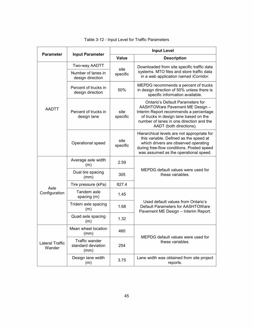
45
Table 3-12 - Input Level for Traffic Parameters
Parameter Input Parameter Input Level
Value Description
AADTT
Two-way AADTT site
specific
Downloaded from site specific traffic data systems. MTO files and store traffic data
in a web application named iCorridor. Number of lanes in
design direction
Percent of trucks in design direction
50% MEPDG recommends a percent of trucks in design direction of 50% unless there is
specific information available.
Percent of trucks in design lane
site specific
Ontario’s Default Parameters for AASHTOWare Pavement ME Design –
Interim Report recommends a percentage of trucks in design lane based on the
number of lanes in one direction and the AADT (both directions).
Operational speed site
specific
Hierarchical levels are not appropriate for this variable. Defined as the speed at which drivers are observed operating
during free-flow conditions. Posted speed was assumed as the operational speed.
Axle Configuration
Average axle width (m)
2.59
MEPDG default values were used for these variables.
Dual tire spacing (mm)
305
Tire pressure (kPa) 827.4
Tandem axle spacing (m)
1.45
Used default values from Ontario’s Default Parameters for AASHTOWare Pavement ME Design – Interim Report.
Tridem axle spacing (m)
1.68
Quad axle spacing (m)
1.32
Lateral Traffic Wander
Mean wheel location (mm)
460
MEPDG default values were used for these variables. Traffic wander
standard deviation (mm)
254
Design lane width (m)
3.75 Lane width was obtained from site project
reports.

46
Table 3-12 - Continued
Parameter Input Parameter Input Level
Value Description
Wheelbase
Short trucks - Average axle spacing (m)
5.1
Used default values from Ontario’s Default Parameters for AASHTOWare Pavement ME Design – Interim Report.
Medium trucks - Average axle spacing (m)
4.6
Long trucks - Average axle spacing (m)
4.7
Percent short trucks 33
MEPDG default values were used for these variables.
Percent medium trucks
33
Percent long trucks 34
Traffic Volume
Adjustment
Vehicle class distribution (Truck
Traffic Classification - TTC)
site specific Downloaded from site specific traffic data
systems. MTO files and store traffic data in a web application named iCorridor.
Traffic Growth Factor
site specific
Monthly and Hourly adjustment
site specific
MEPDG default values were used for these variables.
Axles per truck site
specific Downloaded from site specific traffic data systems. MTO files and store traffic data
in a web application named iCorridor. Axle Load Distribution
Axle distribution (Single, Tandem,
Tridem, Quad)
site specific
Axle-Load Configuration – For the standard truck classes, the spacing of the axles are
relatively constant. The default values listed in Ontario’s Default Parameters for AASHTOWare
Pavement ME Design – Interim Report were used.
Dual Tire Spacing – AASHTOWare software presume that all standard truck axles
contain dual tires. The default value of 305 mm (approx. 12 in) from AASHTOWare was
considered based on the spacing of tires used by the majority of trucks.

47
Tire Pressure – Constant tire pressure is assumed in the AASHTOWare software for all
loading conditions. The default value of 827.4 kPa (approx. 120 psi) from AASHTOWare is
considered, which represents a median operating condition (hot inflation tire pressure).
Lateral Traffic Wander of Axle Loads – Constant wander is assumed in the
AASHTOWare software for all trucks. The default value of 254 mm (approx. 10 in) was used for
calibration procedure, regardless of the lane width.
Mean Wheel Location – is defined as the distance from the pavement marking to the
outer edge of the wheel. The default value of 460 mm (approx. 18 in) is recommended by
AASHTO.
Design Lane Width – is defined as the actual traffic lane width. The existing design lane
width of 3.75 m (approx. 12 ft) was considered.
Wheelbase – the default values for average axle spacing and corresponding truck
percentages for short, medium and long trucks are provided for Ontario’s conditions.
Table 3-13 – Percentage of Trucks in Design Lane (Ontario 2012)
Number of lanes in one direction
AADT (both directions)
Percentage of Trucks in Design Lane
1 All 100
2 <15,000
>15,000
90
80
3
<25,000
25,000 to 40,000
>40,000
80
70
60
4 <40,000
>40,000
70
60
5 <50,000
>50,000
60
60

48
Figure 3-5: Example of Traffic Data Available in iCorridor
Normalized Vehicle (Truck) Class Distribution – represents the percentage of each truck
class (class 4 through 13) within the AADTT for the selected year. The summation of all AADTT
percentages should equal 1.
Traffic Growth Factor (TGF) – represents the annual rate of truck traffic growth over time.
TGF are provided in iCorridor, as a compounded model, for each segment of Provincial
Highways.
Monthly Adjustment Factors - represent the proportion of the annual truck traffic for a
particular truck class that occurs in a given month. During calibration efforts, monthly distribution
factors of 1.0 were used for all classes as defined in the Ontario’s Default Parameters for
AASHTOWare Pavement ME Design – Interim Report.
Number of Axle Types per Truck Class – represents the average number of axles for
each class 4 to 13 for each axle type (single, tandem, tridem and quad). These inputs are
provided in iCorridor, based on the outcome of the CVS 2006 study for Ontario.

49
Figure 3-6: FHWA Vehicle Category Classification (FHWA, 2014)
Axle Load Distribution Factors/Spectra by Truck Class and Axle Type – represent the
percentage of the total axle applications within each load interval for a specific axle type (single,
tandem, tridem and quad) and vehicle class (classes 4 to 13). The normalized axle load
distribution or spectra can only be determined from WIM data (NCHRP, 2004). MTO has

50
developed axle load spectrum tables identifying vehicle classes and axle types based on the CVS
2006 study for Ontario. The Axle Load Spectra data was downloaded from iCorridor in ALF file
format and then converted to Excel format.
3.8.3 Structural Layers and Materials Properties
Materials, layer thickness and properties for each pavement layer were obtained from the
pavement reports provided by MTO. When data was not available, default values tabulated on
the Ontario’s Default Parameters for AASHTOWare Pavement ME Design – Interim Report were
considered. Structure information and materials properties are tabulated in Appendix B.
3.8.3.1 HMA
HMA Layer Thickness – the number of layers, type of material and thicknesses were
obtained from each pavement design report, consulting tables, core and borehole information.
Volumetric Properties of Mixture – default values for unit weight, effective binder content,
air voids and Poisson’s ratio are tabulated on the Ontario’s Default Parameters for AASHTOWare
Pavement ME Design – Interim Report and MEPDG.
Aggregate Gradation – Ontario’s Default Parameters for AASHTOWare Pavement ME
Design – Interim Report provides typical properties for SuperPave and Marshall mixtures.
Dynamic Modulus – in input Level 3, Witczak’s model uses the aggregate gradation to
compute the Dynamic Modulus (E*) of HMA layers.
Asphalt Binder – Ontario’s Default Parameters for AASHTOWare Pavement ME Design –
Interim Report recommends specific penetration grades for a given mixture type.
Thermal - MEPDG default values are used for Thermal Conductivity and Heat Capacity.
The Thermal Contraction is internally computed in MEPDG using the HMA volumetric properties,
such as VMA and the thermal contraction coefficient for the aggregates. Thermal contraction
coefficients are provided for different aggregate types.

51
Table 3-14 - Input Level for Asphalt Concrete material-related variables
Parameter Input Parameter Input Level
Value Description
General HMA Layer Thickness Site
specific Information was obtained from site
project reports.
Structure Surface Shortwave
Absorptivity 0.85
MEPDG default value was used for this variable.
Volumetric Properties of
Mixture
(as built)
Unit Weight (Kg/m3)
Site specific
Used default values from Ontario’s Default Parameters for
AASHTOWare Pavement ME Design – Interim Report.
Effective Binder Content by Volume (%)
Site specific
Air Voids (%) Site
specific
Poisson’s Ratio
Poisson’s Ratio 0.35
Mechanical Properties
Dynamic Modulus Site
specific
Computed using PI and gradation from Project Specific Pavement
Design Reports.
Aggregate Gradation Site
specific
Used default values from Ontario’s Default Parameters for
AASHTOWare Pavement ME Design – Interim Report.
G* Predictive Model3
Site specific
Reference Temperature
(⁰C) 21.1
Asphalt Binder Site
specific
Indirect Tensile Strength at
– 10⁰C (MPa) Site
specific MEPDG calculates parameters based on binder type.
Creep Compliance (1/GPa) Site
specific
Thermal
Thermal Conductivity (W/m-Kelvin)
1.16 MEPDG default value.
Heat Capacity (J/Kg-Kelvin) 963
Thermal Contraction MEPDG calculates parameter
based on HMA properties4.
3 Use Viscosity based model, Nationally calibrated.
4 MEPDG computes internally using the HMA volumetric properties, such as, VMA and the thermal
contraction coefficient for the aggregates. Thermal contraction coefficients are provided for different aggregate types.

52
3.8.3.2 Unbounded Material Properties
Granular Layer Thickness – the number of layers, type of material and thicknesses were
obtained from each pavement design report, after checking the tables with borehole information.
Aggregate Gradation, Liquid Limit and Plastic Index – this data was extracted from
borehole information from each pavement design report.
Resilient Modulus – input Level 2 based on gradation and Plastic Index (PI) was used to
compute the Dynamic Modulus (E*) of unbounded granular materials. Gradation and PI were
obtained from borehole information from each pavement design report.
Additional information about unbound granular material parameters are given in Table
3-4.
3.8.3.3 Subgrade Soil Type and Properties
The soil type and aggregate gradation were extracted from borehole information from
each pavement design report. The Liquid Limit and Plastic Index were available as well. The
Resilient Modulus was included in the pavement design report. However, AASHTOWare
Pavement ME Design was returning an error and thus Level 3 was selected.
Some project reports included the Depth of Ground Water Table from field investigation
testing. For the remaining cases, the default value for Ontario conditions was used, which is
6.1m. Additional information about subgrade material parameters are given in Table 3-5.
3.8.4 Climate Data
AASHTOWare Pavement ME Design integrates processed climate information available
from Environment Canada. There are, currently, 34 weather stations in Ontario. One may select a
single weather station or a set of multiple weather stations in order to create a virtual weather
station. Weather stations are sorted automatically by shortest distance to the project location.
When creating virtual weather stations, more than one weather station must be selected in an
effort to reduce error. By selecting a weather station (single or virtual), the software yields a
climate summary for that location, which includes, mean annual air temperature, mean monthly

53
temperatures (per month), mean annual precipitation, freezing index, average number of
freeze/thaw cycles and number of wet days.
The latitude, longitude and elevation of each project were identified for the purpose of
selecting the nearest weather stations or to create the virtual weather stations from existing
Ontario weather stations.
Due to the limited functionality of the AASHTOWare Pavement ME Design weather
station interpolation function, MTO recommends selecting the closest weather station to the
project (Ontario, 2012).
3.8.5 Pavement Performance Data
The Initial IRI should be measured immediately after construction; however, this
parameter was unavailable in the pavement design reports. The Initial IRI considered for this
research was 0.8 m/km, which is the recommended value for new or reconstructed AC
pavements for freeways tabulated in the Ontario’s Default Parameters for AASHTOWare
Pavement ME Design – Interim Report.
In some cases, it was difficult to assess if the pavement performance data provided was
exactly from the new constructed lane or section in reference. Therefore, assumptions were
made considering that the existing sections were built with identical material properties. The
pavement performance data is tabulated in Appendix C.

54
4 Development of Calibration Models
This chapter presents and describes the development of the procedure to calibrate the
MEPDG performance models (alligator cracking and permanent deformation) for local conditions.
The criteria to proceed with local calibration was based on (a) whether distresses were predicted
without significant bias and (b) whether a given global model demonstrates a reasonable
goodness of fit (between predicted and measured data points). The absence or presence of bias
was assessed based on the hypothesis test described in the following subchapters, while the
reasonable goodness of fit was assessed based on the Standard Error of Estimate (SEE). The
criteria to assess the adequacy of models was defined as shown in Table 4-1.
Table 4-1 – Criteria for Determining Global Models Adequacy
Criterion of
Reference Statistic Test Thresholds Rating
Bias
Hypothesis testing of intercept
of the linear predicted vs
measured distress
p-value for the
intercept
Reject if p-value is
<0.05
Goodness
of fit
SEE, Alligator Cracking model
<5 percent Good
5 to 10 percent Fair
>10 percent Poor
SEE, Total Rutting model
<0.1 in <2.54 mm Good
0.1 to 0.2
in
2.54 to
5.08 mm Fair
>0.2 in > 5.08 mm Poor

55
4.1 Assess Local Bias from Global Calibration Parameters
The AASHTOWare Pavement ME software was run using the global calibration
parameters, for each selected project to predict pavement distresses and IRI over the life of the
project at a 50 percent reliability level.
A comparison was made between the measured and predicted distresses to determine bias,
standard error of estimate and residuals. A linear regression model was used to determine the
correlation between predicted distress (dependent variable, Y) and the measured distress
(independent variable, X). The local bias is assessed by studying the null hypothesis that the bias
(average residual error) is zero at a 95 percent confidence level.
∑( )
Equation (30)
Also, scatter charts of the measured versus the predicted distresses were plotted to
investigate the dispersion of the points in relation to the line of equality.
Table 4-2 – Summary of Statistic Parameters – Global Calibration
Performance Indicator
Regression Coefficients
Mean Error (er)
p-value Hypothesis; ∑( )
Rutting
-7.98 0.462 null hypothesis is not rejected;
p>0.05
Alligator Cracking
3.68 0.083
null hypothesis is not rejected; p>0.05
4.1.1 Assess Local Bias for Alligator Cracking Model
The p-value approach was used to conduct this hypothesis test. The output from
regression gives a p-value of 0.083 which is greater than 0.05. Therefore, the null hypothesis
cannot be rejected. Thus, it cannot be said that the transfer functions produce biased predictions.

56
The plot of measured versus predicted alligator cracking is given in Figure 4-1. The figure
shows a poor linear relationship between measured and predicted distress. The measured cracks
are of much larger magnitude than predicted values, which reflects that the MEPDG model under
predicted alligator cracking. Therefore, the local calibration procedure must be conducted in order
to improve this transfer function.
As shown in Figure 4-1, the intercept is significantly different from zero and the slope
estimator is significantly different from 1. Thus, the transfer function must be calibrated to
local conditions.
Figure 4-1: Measured vs Predicted Alligator Cracking Using Global Calibration Parameters
4.1.2 Assess Local Bias for Rutting Model
The output from regression analysis gives a p-value of 0.462 which is greater than α =
0.05; therefore, the null hypothesis cannot be rejected. Thus, it cannot be stated that the transfer
functions produce biased predictions.
0.00
2.00
4.00
6.00
8.00
10.00
12.00
14.00
0.00 2.00 4.00 6.00 8.00 10.00 12.00 14.00
Me
asu
red
Cra
ckin
g (%
)
Predicted Cracking (%)
Alligator Cracking (%)
AlligatorCracking(%)
Linear(Line ofEquality)

57
The plot of measured versus predicted total rutting was performed. Figure 4-2 shows a
wide dispersion between the measured and predicted rut depths, which suggests a poor
correlation between measured and predicted rutting. Rutting is over predicted using the global
calibration parameters; therefore, local calibration must be conducted for this transfer function.
Also, the intercept is significantly different from zero and the slope estimator is
significantly different from 1. Thus, the transfer function will produce biased predictions and
accordingly should be calibrated to local conditions.
Figure 4-2: Measured vs Predicted Total Rutting Using Global Calibration Parameters
4.2 Eliminate Local Bias of Distress Prediction Models
The procedure to eliminate the bias begins with the identification of the cause for bias.
This is done by adjusting the local calibration coefficients for the biased models. The MEPDG
local calibration coefficients can be amended to reduce bias and/or standard error, as presented
in Table 4-3:
0.0
2.0
4.0
6.0
8.0
10.0
12.0
14.0
16.0
18.0
20.0
0.0 2.0 4.0 6.0 8.0 10.0 12.0 14.0 16.0 18.0 20.0
Me
asu
red
To
tal R
utt
ing
(mm
)
Predicted Total Rutting (mm)
Total Rutting
TotalRutting
Linear(TotalRutting)

58
Table 4-3 – Potential Cause of Bias and Corrective Action (CDOT, 2013)
Potential Cause of Bias Corrective Action
Check and compare predicted against
measured distress/IRI plots for each
individual project in order to identify
projects wherein predicted and
measured values vary significantly.
In case that these projects are a small
percentage, verify data for mistaken inputs and
assumptions and correct them. Then, repeat
process to check if bias was eliminated and use
global coefficients.
Otherwise, iterate global/local coefficients as
required until significant bias is eliminated.
Examine key input variables that
influence each distress type and develop
a residuals plot – predicted/measured
distress versus a particular variable.
Identify trends in the plot. Upward or
downward trends are indicators of
correlation.
Identify and track the global/local coefficients
influencing more the key inputs that relate to
bias. Iterate global/local coefficients as required
until significant bias is eliminated.
Establish that bias is random with not
assigned cause.
Iterate global/local coefficients as required until
significant bias is eliminated
Microsoft Excel Solver and Regression Analysis are used to estimate the calibration
factors of the performance models. The procedure to eliminate the local bias was performed
according to the following steps:
a) The distresses were predicted for the selected projects using the AASHTOWare
Pavement ME Design with the global calibration coefficients;
b) The computed distresses corresponding to the same month and year of performance
data were extracted from ME Design outputs of each project and tabulated along with
measured distresses;
c) The Error, Squared Error, Sum of Squared Errors (SSE) and Standard Error of Estimate
(SEE) were calculated, along with other basic statistics (Mean, Maximum, Minimum and
Standard Deviation);

59
d) Regression Analysis was employed to determine the calibration factors of the rutting
models while Microsoft Excel Solver was used to minimize SSE by adjusting the C1 and
C2 factors of the alligator model.
4.2.1 Eliminate Local Bias for Alligator Cracking Model
The bias of bottom-up fatigue cracking can be improved through four coefficients:
and C2. The C2 term is related with the percentage of area of fatigue cracking from the
damage index, while the beta terms are associated to estimating the allowable number of load
applications for a specific condition and layer. The coefficients and C2 are usually used to
eliminate the model bias and the standard error of the estimate (SEE).
A Microsoft Solver numerical optimization routine was used to find the regression
coefficients C1 and C2. The optimization was set by first predicting, thru AASHTOWare Pavement
ME Design software, the damage for each section, assuming an initial value for C1=1 and C2=1.
Then, by using Equation (8), alligator cracking was computed from the predicted damage
percentage. Then, the predicted alligator cracking was subtracted from the observed alligator
cracking to obtain the error. Then, the errors were squared and summed to obtain the total sum of
squared error (SSE).
At this point, the Microsoft Solver was set to minimize the sum of the squared errors
(SSE) by changing the coefficients C1 and C2 for the first iteration. The first iteration returned
C2=0. When C2 is zero, the computed damage has no effect on the alligator cracking
percentage. Then, Solver was run again and C2 returned negative on the second iteration. When
C2 is negative, more damage leads to less cracking, which is not reasonable. Thence, these runs
were discarded.
At this point, C1 was fixed to 1.0, the original value, and the calibration was continued
only for C2. The local calibration coefficients obtained are: C1 = 1 and C2 = 0.968267 (Table 4-4).

60
Table 4-4 – Computation of the Calibration Coefficients C1 and C2
Measured
MonthPavement
Age (years)
Max
Damage
(%)
Max
Cracking
(%)
hAC (mm) hAC (in) C1' C2'Predicted
Cracking (%)
Total Alligator
Cracking (%)Error |Error| Squared Error
Project 1 10/2014 15.42 0.0468 0.0296 285 11.2205 4.8799 -2.4400 3.5693 9.0622 -5.4930 5.4930 30.1725
Project 2 10/2014 15.42 0.0333 0.0208 290 11.4173 4.8772 -2.4386 2.5492 7.8471 -5.2979 5.2979 28.0675
Project 7 9/2015 10.08 0.0505 0.0330 320 12.5984 4.8635 -2.4318 3.8883 0.8623 3.0259 3.0259 9.1563
Project 11 9/2015 4.08 0.0202 0.0131 440 17.3228 4.8371 -2.4186 1.5953 0.4129 1.1823 1.1823 1.3979
Project 18 9/2015 4.00 0.0254 0.0166 410 16.1417 4.8412 -2.4206 1.9989 0.5014 1.4975 1.4975 2.2424
Project 24 6/2015 5.83 0.0157 0.0096 320 12.5984 4.8635 -2.4318 1.2101 0.3191 0.8910 0.8910 0.7939
Project 27 10/2015 8.25 0.0276 0.0179 375 14.7638 4.8477 -2.4238 2.1607 6.7709 -4.6102 4.6102 21.2540
Project 28 10/2014 17.08 0.0485 0.0323 360 14.1732 4.8511 -2.4256 3.7666 3.5210 0.2455 0.2455 0.0603
Project 38 10/2014 17.08 0.0301 0.0199 435 17.1260 4.8377 -2.4189 2.3733 1.3814 0.9919 0.9919 0.9839
Project 39 10/2014 17.08 0.0515 0.0350 420 16.5354 4.8397 -2.4199 4.0236 4.9978 -0.9742 0.9742 0.9491
Project 41 5/2015 5.83 0.0107 0.0068 450 17.7165 4.8360 -2.4180 0.8433 3.7387 -2.8954 2.8954 8.3836
Project 43 11/2015 6.33 0.0471 0.0313 360 14.1732 4.8511 -2.4256 3.6598 4.9319 -1.2721 1.2721 1.6183
Project 50 9/2015 6.00 0.0186 0.0119 395 15.5512 4.8437 -2.4219 1.4604 0.3349 1.1255 1.1255 1.2667
Project 60 9/2015 8.00 0.0055 0.0029 255 10.0394 4.9010 -2.4505 0.4024 12.6882 -12.2858 12.2858 150.9410
Project 70 8/2015 3.17 0.0077 0.0047 390 15.3543 4.8447 -2.4223 0.6018 0.8366 -0.2348 0.2348 0.0551
Project 81 9/2015 5.00 0.0728 0.0340 160 6.2992 5.0896 -2.5448 4.9019 1.0257 3.8762 3.8762 15.0250
SSE
272.3675
C1 = 1
C2 = 0.968267437
Predicted (from M-E Design) Predicted (by formula)

61
Subsequently, using the local calibration factors, the bottom-up cracking was calculated.
Then, the error for the full set of data was calculated from the difference between predicted
alligator cracking and measured alligator cracking. The errors were squared and then summed to
obtain the total sum of squared error (SSE).
The plot of measured versus predicted alligator cracking, using the local calibration
coefficients, is given in Figure 4-3. This figure shows that the points are randomly scattered along
the equality line and that the predicted values closer to the measured values than in Figure 4-1,
suggesting an improvement in the prediction of alligator cracking.
Figure 4-4 shows that the residual errors are randomly distributed with the exception of
one project. Also, the errors do not increase significantly as the percentage of cracking increases.
The presence of bias between predicted and measured alligator cracking was
investigated through a linear regression analysis between the measured alligator cracking as the
dependent variable and predicted alligator cracking as the independent variable. The p-value of
the intercept was used to test the hypothesis that there is no bias in the prediction. The intercept
in the linear regression would be the bias, the consistent or systematic difference between the
measured and predicted values with the calibrated model. The output from regression (Table 4-5)
gives a p-value of 0.07 which is greater than α = 0.05; therefore, the null hypothesis cannot be
rejected. Thus, for the specified level of confidence, it cannot be stated that the calibrated transfer
function will produce biased predictions.
As shown, the mean error has improved in comparison to the use of the global
calibration values, suggesting that the local calibration procedure has improved the alligator
cracking model.

62
Figure 4-3: Measured vs Predicted Alligator Cracking Using Local Calibration Parameters
Figure 4-4: Residual Error versus Predicted Alligator Cracking
0
2
4
6
8
10
12
14
0 2 4 6 8 10 12 14
Me
asu
red
Cra
ckin
g (%
)
Predicted Cracking (%)
Alligator Cracking (%)
TotalAlligatorCracking(%)
Linear(TotalAlligatorCracking(%))
-14
-12
-10
-8
-6
-4
-2
0
2
4
6
8
10
12
14
0 1 2 3 4 5 6 7 8
Re
sid
ual
Err
or
(%)
Predicted Total Alligator Cracking (%)
Predicted Cracking vs Residual Error
Error

63
Table 4-5 – Summary of Statistic Parameters – Local Calibration
Performance Indicator
Regression Coefficients
Mean Error (er)
p-value Hypothesis;
∑( )
Alligator Cracking
-1.26 % 0.07 null hypothesis
cannot be rejected; p>0.05
4.2.2 Eliminate Local Bias for Rutting Models
There are a total of five calibration factors in the permanent deformation model, three for
the asphalt layers, one for the unbound granular base and another for the unbound subgrade.
These calibration factors are correction constants applied to the initial models to improve the final
calibrated permanent deformation model. The following paragraphs describe the approach used
in the calibration procedure. Note that no trench studies were conducted; therefore, the actual
layer rut depths are not provided. Other mathematical approaches were used instead in this
exercise.
A Microsoft Excel Regression Analysis was used to find the permanent deformation
calibration factors and . The optimization was set by first predicting, through the
AASHTOWare Pavement ME Design software, the rutting for each section after assuming an
initial value for and . The optimization was done using the approach of
minimizing the sum of squared error (SSE) for the rutting in each of the three layers separately.
Therefore, three calibration factors ( and ) were obtained separately. The remaining
calibration coefficients were kept fixed: (temperature) and (number of load
repetitions).
The M-E Design predicts rutting values for the AC, base, subgrade layers and the total
rutting. However, from performance reports, only total rutting is given. In order to address this, the
ratios of rutting in each layer relative to the total rutting was calculated for the rutting values
predicted with the globally calibrated models. Then, the measured total rutting was multiplied by
those ratios to compute the measured rutting values for the AC, base and subgrade layers.

64
After tabulating the ratios for predicted and measured rutting values for the AC, base and
subgrade layers, the local calibration procedure was executed by performing a simple linear
regression, by setting the measured total rutting as the dependent variable (Y) and the predicted
total rutting as the independent variable (X). The intercept was fixed as zero to fit the regression
line through the origin.
The same procedure was carried out for each layer in order to obtain the three calibration
factors, and . The obtained regression coefficients are given in Table 4-6 and
are the local calibration coefficients.
Table 4-6 –Local Calibration Coefficients
Layer Model Regression Coefficients
HMA
Base (
) ( )
Subgrade (
) ( )
After that, using the local calibration factors, the total rutting was calculated using
Equations (16) and (21). Then, the residual error for the full set of data was calculated as the
difference between predicted total rutting and measured total rutting. The SSE was then obtained
from the squared errors.
The plot of measured versus predicted rutting in each layer of the pavement, using the
local calibration coefficients, was performed as shown in Figure 4-5 to Figure 4-11. The
measured total rutting versus the predicted total rutting was also plotted.

65
Figure 4-5: Measured vs Predicted AC Rutting Using Global Calibration Parameters
Figure 4-6: Measured vs Predicted AC Rutting Using Local Calibration Parameters
0.0
1.0
2.0
3.0
4.0
5.0
6.0
7.0
8.0
0.0 1.0 2.0 3.0 4.0 5.0 6.0 7.0 8.0
Me
asu
red
AC
(m
m)
Predicted AC (mm)
Rutting AC Layer (Global)
0.0
0.5
1.0
1.5
2.0
2.5
3.0
3.5
4.0
4.5
5.0
0.0 1.0 2.0 3.0 4.0 5.0
Me
asu
red
AC
(m
m)
Predicted AC (mm)
Rutting AC Layer (Local)

66
Figure 4-7: Measured vs Predicted Base Rutting Using Global Calibration Parameters
Figure 4-8: Measured vs Predicted Base Rutting Using Local Calibration Parameters
0.0
1.0
2.0
3.0
0.0 1.0 2.0 3.0
Me
asu
red
Bas
e (
mm
)
Predicted Base (mm)
Rutting Base Layer (Global)
0.0
1.0
2.0
3.0
0.0 1.0 2.0 3.0
Me
asu
red
Bas
e (
mm
)
Predicted Base (mm)
Rutting Base Layer (Local)

67
Figure 4-9: Measured vs Predicted Subgrade Rutting Using Global Calibration Parameters
Figure 4-10: Measured vs Predicted Subgrade Rutting Using Local Calibration Parameters
0.0
1.0
2.0
3.0
4.0
5.0
6.0
7.0
8.0
9.0
10.0
0.0 1.0 2.0 3.0 4.0 5.0 6.0 7.0 8.0 9.0 10.0
Me
asu
red
Su
bgr
ade
(m
m)
Predicted Subgrade (mm)
Rutting Subgrade Layer (Global)
0.0
1.0
2.0
3.0
4.0
5.0
6.0
0.0 1.0 2.0 3.0 4.0 5.0 6.0
Me
asu
red
Su
bgr
ade
(m
m)
Predicted Subgrade (mm)
Rutting Subgrade Layer (Local)
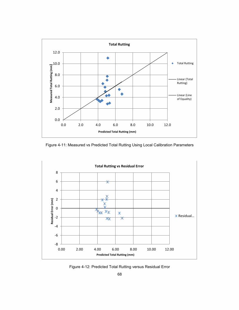
68
Figure 4-11: Measured vs Predicted Total Rutting Using Local Calibration Parameters
Figure 4-12: Predicted Total Rutting versus Residual Error
0.0
2.0
4.0
6.0
8.0
10.0
12.0
0.0 2.0 4.0 6.0 8.0 10.0 12.0
Me
asu
red
To
tal R
utt
ing
(mm
)
Predicted Total Rutting (mm)
Total Rutting
Total Rutting
Linear (TotalRutting)
Linear (Lineof Equality)
-8
-6
-4
-2
0
2
4
6
8
0.00 2.00 4.00 6.00 8.00 10.00 12.00
Re
sid
ual
Err
or
(mm
)
Predicted Total Rutting (mm)
Total Rutting vs Residual Error
Residual…

69
Figure 4-5 to Figure 4-11 show that the local calibration coefficients provide a better fit
between predicted and measured rutting, in all layers separately and for the total rutting, which
means that the prediction of permanent deformation has improved. Lastly, Figure 4-12 shows that
the residual errors are randomly distributed and not correlated to the predicted rutting.
The presence of bias between the predicted and measured total rutting was investigated
through a linear regression analysis between the measured total rutting as the dependent
variable and predicted total rutting as the independent variable. The p-value of the intercept was
used to test the hypothesis that there is no bias in the prediction. The intercept in the linear
regression would be the bias, the consistent or systematic difference between the measured and
predicted total rutting with the calibrated model. The output from regression (Table 4-7) shows a
p-value for the intercept of 0.49, which is much greater than α = 0.05; therefore, the null
hypothesis cannot be rejected. Thus, for the specified level of confidence, it cannot be stated that
the transfer function will produce biased predictions.
The average error or bias was reduced and the accuracy of the transfer function has
increased in comparison to the use of the global calibration values, suggesting that the local
calibration procedure has improved the rutting model.
Table 4-7 – Summary of Statistic Parameters – Local Calibration
Performance Indicator
Regression Coefficients
Mean Error (er)
p-value Hypothesis;
∑( )
Rutting
0.09 mm 0.49
null hypothesis
cannot be rejected;
p>0.05

70
4.3 Assess the Goodness of Fit
In order to assess the goodness of fit, the standard error of the estimate (SEE) was
obtained from the analysis performed in subchapter 4.2 (Microsoft Excel Solver and Regression
Analysis) following the determination of the SSE. Then, these parameters were compared with
the parameters from global calibration models, as shown in Table 4-8.
Table 4-8 – MEPDG Statistic Parameters – Global and Local Calibration
Performance Model
Mean Error (er) Standard Error of Estimate (SEE)
Global Local Global Local
Total
Rutting -7.98 mm 0.09 mm 8.68 mm 2.17 mm
Alligator
Cracking 3.68 % -1.26% 5.35 % 4.26 %
The standard error of estimate is the main indicator to measure if the model improved or
not. Table 4-8 shows that using local calibration coefficients, the standard error of estimate (SEE)
for alligator cracking improved slightly from 5.35 to 4.26 percent of lane area. With regard to
rutting model, the SEE improved significantly from 8.68 to 2.17 mm. It can be concluded that local
calibration procedure has improved the prediction models. In addition, SEE parameters are
considered good when compared with thresholds defined in Table 4-1.
In the case of alligator cracking, in order to improve accuracy and precision of the models,
more data is required, in particular, more pavement sections exhibiting higher level of distresses.

71
5 Summary, Conclusions and Recommendations
5.1 Summary
The primary objective of this project was to calibrate the performance models used in the
AASHTOWare Pavement ME for the design of new flexible pavement structures to local
conditions of Ontario, Canada, considering local traffic conditions, materials properties and
structure information from pavement design reports and local climate information. MTO pavement
management database was a major source for traffic, field-testing structural information and
performance data. For climatic data, local weather stations embedded in AASHTOWare software
were considered.
The calibration procedure followed the Guide for Mechanistic-Empirical Design
(AASHTO, 2008) and guidelines in the Ontario’s Default Parameters for AASHTOWare Pavement
ME Design – Interim Report (Ontario’s Interim Report, 2012). The AASHTOWare Pavement ME
DesignTM
software was used to predict pavement distresses.
This research deals only with new flexible pavement structures. Sixteen (16) representative
pavement sections were selected from widening and reconfiguration highway projects, combining
a variety of pavement structures, subgrade soils, materials properties and traffic conditions.
These sections, with pavement ages ranging from 3 to 17 years, include also a variety of distress
levels.
5.2 Conclusions
The pavement distress models evaluated and calibrated in this research are (i) total
rutting and (ii) AC bottom-up fatigue cracking. The calibration procedure includes the comparison
between measured (from performance data) and predicted values (from M-E Design software).
The statistical analysis showed that, using the global calibration coefficients, the AASHTOWare
models under predicted alligator cracking and over predicted total rutting.

72
An optimization process was undertaken to obtain the calibration coefficients for the
bottom-up fatigue cracking model, C1 and C2. The final coefficients obtained for local calibration
were: C1 = 1 and C2 = 0.968267. The local calibration factors have improved the mean prediction
error (from 3.68 to -1.26) and standard error of the estimate (from 5.35 to 4.26).
The plot of measured versus predicted alligator cracking, showed that the predicted
values moved closer to the measured values due to the local calibration. In addition, the statistical
analysis could not state that the transfer function will produce biased predictions, at the specified
level of confidence.
However, one possible justification for the slight improvement in SEE could be the
measurement procedure used by the agency. The agency measures and records alligator
cracking in 3 different categories (slight, moderate and severe) and in 3 different places within the
traffic lane (mid lane, edge of pavement and wheel path). The total area of alligator cracking is
obtained by the summation of all six values without applying any weighting factor. Finally, it is
important to recall that this research deals with Provincial Highways (fairly compared to Interstate
Highways in the United States). Therefore, high percentages of alligator cracking are not
expected due to the high design standards and the strict rehabilitation program.
Regression analysis was performed to find the following coefficients for the local
calibration of the rutting model: and . The
local calibration factors have improved bias (from -7.98 to 0.09), and reduced the standard error
of the estimate (from 8.68 to 2.17). Using the local calibration coefficients, the average error or
bias was reduced and the accuracy of transfer function has increased in comparison to the use of
the global calibration values, suggesting that the local calibration procedure has improved the
rutting model.

73
5.3 Recommendations
This research led to the following recommendations for future research:
(i) The database used in this research was selected from widening and reconfiguration
highway projects, combining a variety of pavement structures, subgrade soils, materials
properties, traffic conditions and a variety of distress levels. In order to enhance the
models, improve accuracy and precision, more data is required, in particular, for new
pavement sections that are closer to failure.
(ii) Trench studies would be recommended in order to determine the contribution of each layer
to total rutting.
(iii) Finally, transverse cracking data should be collected in order to allow the calibration of the
thermal cracking models to local conditions.

74
Appendix A
Traffic Data

75
Table A-1 - Traffic Inputs
Project # AADTT
Number of Lanes in Design
Direction
% of Trucks in Design
Lane
Operational Speed (Km/h)
AADTT Growth Rate
(%)
1 3,200 2 80 70 2.15
2 3,000 2 80 70 2.15
7 11,200 3 60 100 2.78
11 17,400 3 60 100 2.05
18 22,000 3 60 100 2.08
24 4,520 2 80 100 2.51
27 11,560 2 80 100 2.08
28 12,000 3 60 100 2.09
38 20,546 3 60 100 2.43
39 20,546 3 60 100 2.43
41 23,400 3 60 100 2.42
43 20,600 3 60 100 2.43
50 18,000 3 60 100 2.06
60 414 1 100 70 2.94
70 9,040 3 60 100 2.35
81 528 1 100 70 2.57

76
Table A-2 - Distribution by Vehicle Class (%)
Project #
Vehicle Class
4 5 6 7 8 9 10 11 12 13
1 1.50 14.12 8.21 4.36 1.65 44.88 22.63 0.00 0.00 2.65
2 1.50 14.12 8.21 4.36 1.65 44.93 22.58 0.00 0.00 2.65
7 1.00 8.22 5.37 0.56 1.27 55.69 23.29 0.40 0.20 4.00
11 2.00 17.92 7.95 2.38 1.74 43.59 21.61 0.26 0.19 2.36
18 2.00 18.45 9.36 3.97 1.98 40.29 20.78 0.25 0.17 2.75
24 1.50 13.43 5.29 1.76 1.29 42.81 24.76 0.00 0.20 8.96
27 1.50 13.77 5.84 0.65 1.12 50.98 23.08 0.19 0.13 2.74
28 1.50 16.32 6.77 2.10 1.46 44.87 23.22 0.13 0.13 3.50
38 1.50 10.14 7.60 2.35 1.72 53.60 20.50 0.17 0.17 2.25
39 1.50 10.14 7.60 2.35 1.72 53.60 20.50 0.17 0.17 2.25
41 1.50 10.20 7.57 2.16 1.71 54.10 20.12 0.17 0.17 2.30
43 1.50 10.13 7.58 2.27 1.70 53.93 20.26 0.17 0.17 2.29
50 2.00 18.45 8.98 3.66 1.87 41.64 20.65 0.24 0.18 2.33
60 0.75 15.61 25.36 0.00 9.76 21.69 22.93 0.00 0.00 3.90
70 1.50 18.94 10.03 4.05 1.57 34.58 22.71 0.13 0.18 6.31
81 0.75 23.19 10.14 0.00 0.00 22.44 33.33 0.00 2.90 7.25

77
Table A-3 - Number of Axles per Truck
Project # Axles
Vehicle Class
4 5 6 7 8 9 10 11 12 13
1
Single 1.62 2.00 1.01 1.41 2.00 1.12 1.62 0.00 0.00 1.15
Tandem 0.39 0.00 0.99 0.99 0.97 1.94 1.41 0.00 0.00 2.08
Tridem 0.00 0.00 0.00 0.02 0.00 0.00 0.56 0.00 0.00 0.74
Quad 0.00 0.00 0.00 0.00 0.00 0.00 0.04 0.00 0.00 0.04
2
Single 1.62 2.00 1.01 1.41 2.00 1.12 1.62 0.00 0.00 1.15
Tandem 0.39 0.00 0.99 0.99 0.97 1.94 1.42 0.00 0.00 2.08
Tridem 0.00 0.00 0.00 0.02 0.00 0.00 0.56 0.00 0.00 0.74
Quad 0.00 0.00 0.00 0.00 0.00 0.00 0.04 0.00 0.00 0.04
7
Single 1.62 2.00 1.01 1.09 2.14 1.04 1.26 4.28 2.80 1.11
Tandem 0.39 0.00 0.99 0.88 0.88 1.98 1.13 0.25 1.60 2.08
Tridem 0.00 0.00 0.00 0.14 0.00 0.00 0.85 0.00 0.00 0.86
Quad 0.00 0.00 0.00 0.00 0.00 0.00 0.04 0.00 0.00 0.02
11
Single 1.62 2.00 1.01 1.36 2.09 1.05 1.44 4.49 2.85 1.14
Tandem 0.39 0.00 0.99 0.99 0.91 1.97 1.26 0.14 1.50 2.04
Tridem 0.00 0.00 0.00 0.02 0.00 0.00 0.68 0.00 0.00 0.88
Quad 0.00 0.00 0.00 0.00 0.00 0.00 0.08 0.00 0.00 0.03
18
Single 1.62 2.00 1.02 1.30 2.12 1.04 1.42 4.46 2.85 1.28
Tandem 0.39 0.00 0.99 0.99 0.89 1.97 1.25 0.22 1.50 2.06
Tridem 0.00 0.00 0.00 0.02 0.00 0.00 0.70 0.00 0.00 0.79
Quad 0.00 0.00 0.00 0.00 0.00 0.00 0.08 0.00 0.00 0.02
24
Single 1.62 2.00 1.01 1.39 2.68 1.05 1.44 0.00 3.00 1.05
Tandem 0.39 0.00 1.00 1.00 0.58 1.95 1.30 0.00 1.00 2.04
Tridem 0.00 0.00 0.00 0.00 0.00 0.02 0.72 0.00 0.00 0.94
Quad 0.00 0.00 0.00 0.00 0.00 0.00 0.07 0.00 0.00 0.01
27
Single 1.62 2.00 1.01 1.27 2.06 1.10 1.55 4.44 3.00 1.58
Tandem 0.39 0.00 0.99 0.97 0.98 1.95 1.31 0.33 1.67 1.92
Tridem 0.00 0.00 0.00 0.03 0.00 0.00 0.54 0.00 0.00 0.89
Quad 0.00 0.00 0.00 0.00 0.00 0.00 0.19 0.00 0.00 0.02
28
Single 1.62 2.00 1.00 1.47 2.04 1.08 1.47 4.63 2.63 1.26
Tandem 0.39 0.00 1.00 0.94 0.96 1.96 1.25 0.00 1.63 1.99
Tridem 0.00 0.00 0.00 0.05 0.00 0.00 0.64 0.00 0.00 0.89
Quad 0.00 0.00 0.00 0.00 0.00 0.00 0.13 0.00 0.00 0.03

78
Table A-3 - Number of Axles per Truck (Continued)
Project # Axles
Vehicle Class
4 5 6 7 8 9 10 11 12 13
38
Single 1.62 2.00 1.01 1.32 2.12 1.03 1.41 4.77 2.94 1.32
Tandem 0.39 0.00 0.99 0.99 0.87 1.98 1.37 0.14 1.47 2.13
Tridem 0.00 0.00 0.00 0.03 0.00 0.00 0.59 0.00 0.00 0.72
Quad 0.00 0.00 0.00 0.00 0.00 0.00 0.09 0.00 0.00 0.03
39
Single 1.62 2.00 1.01 1.32 2.12 1.03 1.41 4.77 2.94 1.32
Tandem 0.39 0.00 0.99 0.99 0.87 1.98 1.37 0.14 1.47 2.13
Tridem 0.00 0.00 0.00 0.03 0.00 0.00 0.59 0.00 0.00 0.72
Quad 0.00 0.00 0.00 0.00 0.00 0.00 0.09 0.00 0.00 0.03
41
Single 1.62 2.00 1.01 1.32 2.13 1.03 1.41 4.77 2.94 1.32
Tandem 0.39 0.00 0.99 0.99 0.87 1.98 1.37 0.15 1.47 2.13
Tridem 0.00 0.00 0.00 0.03 0.00 0.00 0.59 0.00 0.00 0.71
Quad 0.00 0.00 0.00 0.00 0.00 0.00 0.09 0.00 0.00 0.03
43
Single 1.62 2.00 1.01 1.32 2.13 1.03 1.41 4.77 2.94 1.32
Tandem 0.39 0.00 0.99 0.99 0.87 1.98 1.37 0.14 1.47 2.14
Tridem 0.00 0.00 0.00 0.04 0.00 0.00 0.59 0.00 0.00 0.71
Quad 0.00 0.00 0.00 0.00 0.00 0.00 0.09 0.00 0.00 0.03
50
Single 1.62 2.00 1.03 1.30 2.10 1.04 1.42 4.49 2.85 1.13
Tandem 0.39 0.00 0.98 0.99 0.89 1.97 1.25 0.14 1.50 2.05
Tridem 0.00 0.00 0.00 0.02 0.00 0.00 0.70 0.00 0.00 0.87
Quad 0.00 0.00 0.00 0.00 0.00 0.00 0.08 0.00 0.00 0.03
60
Single 1.62 2.00 1.00 0.00 3.80 1.41 1.51 0.00 0.00 1.38
Tandem 0.39 0.00 1.00 0.00 0.00 1.80 1.45 0.00 0.00 1.75
Tridem 0.00 0.00 0.00 0.00 0.00 0.00 0.60 0.00 0.00 1.13
Quad 0.00 0.00 0.00 0.00 0.00 0.00 0.00 0.00 0.00 0.00
70
Single 1.62 2.00 1.00 1.21 2.24 1.06 1.46 5.00 2.55 1.08
Tandem 0.39 0.00 1.00 0.98 0.76 1.95 1.30 0.13 1.73 2.02
Tridem 0.00 0.00 0.00 0.02 0.00 0.02 0.67 0.00 0.00 0.93
Quad 0.00 0.00 0.00 0.00 0.00 0.00 0.06 0.00 0.00 0.01
81
Single 1.62 2.00 1.00 0.00 0.00 1.13 1.48 0.00 1.00 1.40
Tandem 0.39 0.00 1.00 0.00 0.00 2.00 1.30 0.00 1.50 1.20
Tridem 0.00 0.00 0.00 0.00 0.00 0.00 0.74 0.00 0.00 1.00
Quad 0.00 0.00 0.00 0.00 0.00 0.00 0.00 0.00 0.00 0.00

79
Appendix B
Pavement Structure Information

80
Table B-1 - Pavement Structure Information
150
mm
26.5
mm
19
mm
13.2
mm
9.5
mm
4.75
mm
(#4)
2 mm
(#10)
1.18
mm
0.425
mm
(#40)
0.300
mm
0.075
mm
(#200)
0.05
mm
0.02
mm
1 DFC 45 100 82.5 52.5 2.5 2520 3.5 12.4 85-100
2 HDBC 105 97 63 43.5 3 2460 4 10.9 85-100
3 HL8 135 97 63 42.5 3 2460 4 10.9 85-100
4 GrA 125 100 100 92 78 66 45 27 14 6 6 0 194
5 GrB 790 100 100 75 37 21 13 11 11 0 194
6 CL Semi-infinite 94 91 83 70 33 24 27 15 12 35 6.1
1 DFC 50 100 82.5 52.5 2.5 2520 3.5 12.4 85-100
2 HDBC 120 97 63 43.5 3 2460 4 10.9 85-100
3 HL8 120 97 63 42.5 3 2460 4 10.9 85-100
4 GrA 190 100 100 100 98 92 69 32 13 6 6 0 215
5 GrB 590 100 75 60 55 33.5 4 11 11 0 215
6 CL Semi-infinite 96 94 86 67 30 24 29 17 12 35 6.1
1 SP 12.5 40 100 83.2 54 4 2460 4 11.8 PG 64-28
2 SP 19 100 100 96.9 72.5 52.8 3.9 2460 4 11.2 PG 58-28
3 SP 25 180 100 89.1 63.3 49.3 3.8 2469 4 10.4 PG 58-28
4 GrA 300 100 100 78 67 53 36 18 8 6 6 0 250
5 GrB 380 100 100 68 52 30 6 11 11 0 250
6 ML Semi-infinite 97 94 87 59 18 14 12 10 2 35 6.1
1 SP 12.5 100 100 83.2 54 4 2460 4 11.8 PG 64-28
2 SP 19 160 100 96.9 72.5 52.8 3.9 2460 4 11.2 PG 58-28
3 SP 25 180 100 89.1 63.3 49.3 3.8 2469 4 10.4 PG 58-28
4 GrB 380 96 92 89 84 77 66 56 49 11 11 0 128
5 CI Semi-infinite 90 84 77 71 38 29 41 20 21 30 6.1
1 SP 12.5 50 100 83.2 54 4 2460 4 11.8 PG 64-28
2 SP 19 160 100 96.9 72.5 52.8 3.9 2460 4 11.2 PG 58-28
3 SP 25 200 100 89.1 63.3 49.3 3.8 2469 4 10.4 PG 58-28
4 GrB 490 96 92 89 84 77 66 56 49 11 11 0 128
5 CH Semi-infinite 82 59 32 24 39 19 20 50 6.1
1 SP 12.5 50 100 83.2 54 4 2460 4 11.8 PG 64-28
2 SP 19 120 100 96.9 72.5 52.8 3.9 2460 4 11.2 PG 58-28
3 SP 19 150 100 96.9 72.5 52.8 3.9 2460 4 11.2 PG 58-28
4 GrA 520 100 88 80 69 59 46 23 9 6 6 0 216
5 GrB 200 100 89 77 63 33 12 11 11 0
6 SM Semi-infinite 99 98 87 42 16 12 18 14 4 30 1.3
QEW from Winston
Churchill Blvd to
Trafalgar Rd (WBL4)
18
24400 from Hwy 11 to
Hwy 93 (Simcoe County)
2Hwy 6 from Hwy 5 to
Concession 6 W
7401 at Newcastle EB
(L3)
QEW from Brant St to
Burloak Dr (L3)11
1Hwy 6 from Hwy 5 to
Concession 6 W
Unit
Weight
(Kg/m3)
Va
(%)
Vbe
(%)
% Passing
Project
#Project Description
Layer
Number
Layer
Type
Representative
Thickness (mm)
Plastic
Limit
(PL)
Plastic
Index
(PI)
Resilient
Modulus
(Mpa)
Groundwater
Table Depth
(m)
Asphalt
Binder
Liquid
Limit
(LL)

81
Table B-1 - Pavement Structure Information (Continued)
150
mm
26.5
mm
19
mm
13.2
mm
9.5
mm
4.75
mm
(#4)
2 mm
(#10)
1.18
mm
0.425
mm
(#40)
0.300
mm
0.075
mm
(#200)
0.05
mm
0.02
mm
1 DFC 55 100 82.5 52.5 2.5 2520 3.5 12.4 85-100
2 HDBC 90 97 63 43.5 3 2460 4 10.9 85-100
3 HL8 230 97 63 42.5 3 2460 4 10.9 85-100
4 GrA 460 100 99 59 42 21 7 6 6 0 215
5 CL Semi-infinite 100 99 92 83 19 15 26 19 7 35 6.1
1 DFC 50 100 82.5 52.5 2.5 2520 3.5 12.4 85-100
2 HDBC 150 97 63 43.5 3 2460 4 10.9 85-100
3 HL8 160 97 63 42.5 3 2460 4 10.9 85-100
4 GrA 690 100 100 81 66 51 30 19 13 6 6 0 234
5 CL-ML Semi-infinite 76 64 57 54 24 17 21 14 7 25 6.1
1 DFC 40 100 82.5 52.5 2.5 2520 3.5 12.4 85-100
2 HDBC 185 97 63 43.5 3 2460 4 10.9 85-100
3 HL8 210 100 97 63 42.5 3 2460 4 10.9 85-100
4 GrA 330 100 92 85 78 59 39 24 16 6 6 0 215
5 GrB 300 100 75 60 55 33.5 4 11 10 1 215
6 CI Semi-infinite 99 96 89 79 47 34 39 20 19 30 6.1
1 DFC 40 100 82.5 52.5 2.5 2520 3.5 12.4 85-100
2 HDBC 180 97 63 43.5 3 2460 4 10.9 85-100
3 HL8 200 97 63 42.5 3 2460 4 10.9 85-100
4 GrA 350 100 100 88 77 61 41 25 16 6 6 0 250
5 GrB 300 100 75 60 55 33.5 4 11 10 1 250
6 CL-CI Semi-infinite 93 91 84 75 41 33 36 21 15 30 6.1
1 SP 12.5 60 100 83.2 54 4 2460 4 11.8 PG 64-28
2 SP 19 200 100 96.9 72.5 52.8 3.9 2460 4 11.2 PG 58-28
3 SP 19 190 100 96.9 72.5 52.8 3.9 2460 4 11.2 PG 58-28
4 GrA 400 100 95 86 78 58 38 24 15 6 6 0 216
5 GrB 250 100 75 60 55 33.5 4 14 12 2 215
6 CI Semi-infinite 94 92 87 76 42 30 38 17 21 30 6.1
1 SP 12.5 60 100 83.2 54 4 2460 4 11.8 PG 64-28
2 SP 19 160 100 96.9 72.5 52.8 3.9 2460 4 11.2 PG 58-28
3 SP 25 140 100 89.1 63.3 49.3 3.8 2469 4 10.4 PG 58-28
4 GrA 240 100 100 87 76 55 34 23 14 6 6 0 221
5 GrB 280 100 100 71 45 30 18 11 11 0 221
6 CI Semi-infinite 97 94 90 78 44 33 40 16 24 30 1.3
Plastic
Index
(PI)
Resilient
Modulus
(Mpa)
Groundwater
Table Depth
(m)
Va
(%)
Vbe
(%)
Asphalt
Binder
Liquid
Limit
(LL)
Plastic
Limit
(PL)
Layer
Number
Layer
Type
Representative
Thickness (mm)
% PassingUnit
Weight
(Kg/m3)
41401 from Credit River to
Trafalgar Rd (EB)
43401 from Credit River to
Trafalgar Rd (WB)
28403 from Aberdeen
Avenue to York Blvd (EB)
38401 from Trafalgar Rd
to Regional Rd 25 (EB)
39401 from Trafalgar Rd
to Regional Rd 25 (WB)
27403 Fiddler's Green
Road Interchange
Project
#Project Description

82
Table B-1 - Pavement Structure Information (Continued)
150
mm
26.5
mm
19
mm
13.2
mm
9.5
mm
4.75
mm
(#4)
2 mm
(#10)
1.18
mm
0.425
mm
(#40)
0.300
mm
0.075
mm
(#200)
0.05
mm
0.02
mm
1 SP 12.5 45 100 83.2 54 4 2460 4 11.8 PG 64-28
2 SP 19 120 100 96.9 72.5 52.8 3.9 2460 4 11.2 PG 58-28
3 SP 19 230 100 96.9 72.5 52.8 3.9 2460 4 11.2 PG 58-28
4 GrA 495 100 100 93 88 72 44 26 16 6 6 0 186
5 CL Semi-infinite 100 88 35 33 18 15 30 6.1
1 HL1 40 100 82.5 55 2.5 2520 4 12.4 85-100
2 HL2 110 100 100 92.5 5.5 2410 5 14.2 85-100
3 HL4 105 100 72 53.5 3 2480 4 12.2 85-100
4 GrA 255 100 93 78 62 45 28 14 5 6 6 0 245
5 SW-SM 405 100 94 84 75 59 30 11 18 14 4 65
6 SM Semi-infinite 100 97 95 93 90 82 65 41 29 20 18 14 4 25 6.1
1 SP 12.5 40 100 83.2 54 4 2460 4 11.8 PG 64-28
2 SP 19 185 100 96.9 72.5 52.8 3.9 2460 4 11.2 PG 58-28
3 SP 25 165 100 89.1 63.3 49.3 3.8 2469 4 10.4 PG 58-28
4 GrA 320 100 97 93 85 67 51 32 18 6 6 0 185
5 GrB 590 100 100 98 97 80 8 11 11 0 185
6 CL Semi-infinite 100 99 96 73 35 23 26 14 12 30 6.1
1 SP 12.5 30 100 83.2 54 4 2460 4 11.8 PG 64-28
2 SP 19 70 100 96.9 72.5 52.8 3.9 2460 4 11.2 PG 58-28
3 SP 19 60 100 96.9 72.5 52.8 3.9 2460 4 11.2 PG 58-28
4 GrB 500 100 100 60 46 24 10 11 11 0 213
5 CL Semi-infinite 96 58 28 21 27 15 12 35 6.1
Resilient
Modulus
(Mpa)
Groundwater
Table Depth
(m)
Project
#Project Description
Layer
Number
Layer
Type
Representative
Thickness (mm)
% PassingUnit
Weight
(Kg/m3)
Va
(%)
Vbe
(%)
Asphalt
Binder
Liquid
Limit
(LL)
Plastic
Limit
(PL)
Plastic
Index
(PI)
60Hwy 12 from County Rd
23 to City of Orillia
70400 from King Road to
South Canal Bridge (SB)
81
Hwy 12 from Rama Rd
to Simcoe/Durham
Boundary
50QEW from Third Line to
Burloak Drive (EB)

83
Appendix C
Pavement Performance Data

84
Table C-1 - Pavement Performance Data
Project #
Total Section
Length (m)
Highway Designation
Average Total
Rutting (mm)
Average Total
Rutting (in)
Total Area of Alligator
Cracking in the section (m2)
Total Area of section
(m2)
Total Alligator Cracking
(%)
1 6,025 6 7.736 0.30 2,047 22,592 9.062%
2 6,100 6 7.056 0.28 1,795 22,875 7.847%
7 11,634 401 4.585 0.18 376 43,629 0.862%
11 2,926 1 3.250 0.13 45 10,972 0.413%
18 3,004 1 3.468 0.14 56 11,267 0.501%
24 9,738 400 2.972 0.12 117 36,518 0.319%
27 7,473 403 4.280 0.17 1,897 28,023 6.771%
28 2,950 403 10.997 0.43 390 11,063 3.521%
38 9,450 401 2.834 0.11 490 35,438 1.381%
39 9,268 401 5.394 0.21 1,737 34,755 4.998%
41 2,404 401 6.444 0.25 337 9,014 3.739%
43 2,193 401 4.364 0.17 406 8,224 4.932%
50 5,032 1 5.798 0.23 63 18,871 0.335%
60 5,542 12 5.057 0.20 2,637 20,783 12.688%
70 12,308 400 3.646 0.14 386 46,156 0.837%
81 15,954 12 3.446 0.14 614 59,829 1.026%

85
Appendix D
Predicted Distresses from AASHTOWare and Calculations

86
Table D-1 - Global Calibration - Predicted Alligator Cracking
MonthPavement
Age (years)
Max
Damage
(%)
Max
Cracking
(%)
hAC (mm) hAC (in) C1' C2'Predicted
Cracking (%)
1 10/2014 15.42 0.0468 0.0296 285 11.2205 4.8799 -2.4400 0.0296
2 10/2014 15.42 0.0333 0.0208 290 11.4173 4.8772 -2.4386 0.0207
7 9/2015 10.08 0.0505 0.0330 320 12.5984 4.8635 -2.4318 0.0330
11 9/2015 4.08 0.0202 0.0131 440 17.3228 4.8371 -2.4186 0.0132
18 9/2015 4.00 0.0254 0.0166 410 16.1417 4.8412 -2.4206 0.0166
24 6/2015 5.83 0.0157 0.0096 320 12.5984 4.8635 -2.4318 0.0096
27 10/2015 8.25 0.0276 0.0179 375 14.7638 4.8477 -2.4238 0.0179
28 10/2014 17.08 0.0485 0.0323 360 14.1732 4.8511 -2.4256 0.0323
38 10/2014 17.08 0.0301 0.0199 435 17.1260 4.8377 -2.4189 0.0200
39 10/2014 17.08 0.0515 0.0350 420 16.5354 4.8397 -2.4199 0.0350
41 5/2015 5.83 0.0107 0.0068 450 17.7165 4.8360 -2.4180 0.0068
43 11/2015 6.33 0.0471 0.0313 360 14.1732 4.8511 -2.4256 0.0313
50 9/2015 6.00 0.0186 0.0119 395 15.5512 4.8437 -2.4219 0.0119
60 9/2015 8.00 0.0055 0.0029 255 10.0394 4.9010 -2.4505 0.0029
70 8/2015 3.17 0.0077 0.0047 390 15.3543 4.8447 -2.4223 0.0047
81 9/2015 5.00 0.0728 0.0340 160 6.2992 5.0896 -2.5448 0.0340
C1 = 1
C2 = 1
Predicted (from M-E Design) Predicted (by formula)
Project #

87
Table D-2 - Local Calibration - Predicted Alligator Cracking
MonthPavement
Age (years)
Max
Damage
(%)
Max
Cracking
(%)
hAC (mm) hAC (in) C1' C2'Predicted
Cracking (%)
1 10/2014 15.42 0.0468 0.0296 285 11.2205 4.8799 -2.4400 3.5693
2 10/2014 15.42 0.0333 0.0208 290 11.4173 4.8772 -2.4386 2.5492
7 9/2015 10.08 0.0505 0.0330 320 12.5984 4.8635 -2.4318 3.8883
11 9/2015 4.08 0.0202 0.0131 440 17.3228 4.8371 -2.4186 1.5953
18 9/2015 4.00 0.0254 0.0166 410 16.1417 4.8412 -2.4206 1.9989
24 6/2015 5.83 0.0157 0.0096 320 12.5984 4.8635 -2.4318 1.2101
27 10/2015 8.25 0.0276 0.0179 375 14.7638 4.8477 -2.4238 2.1607
28 10/2014 17.08 0.0485 0.0323 360 14.1732 4.8511 -2.4256 3.7666
38 10/2014 17.08 0.0301 0.0199 435 17.1260 4.8377 -2.4189 2.3733
39 10/2014 17.08 0.0515 0.0350 420 16.5354 4.8397 -2.4199 4.0236
41 5/2015 5.83 0.0107 0.0068 450 17.7165 4.8360 -2.4180 0.8433
43 11/2015 6.33 0.0471 0.0313 360 14.1732 4.8511 -2.4256 3.6598
50 9/2015 6.00 0.0186 0.0119 395 15.5512 4.8437 -2.4219 1.4604
60 9/2015 8.00 0.0055 0.0029 255 10.0394 4.9010 -2.4505 0.4024
70 8/2015 3.17 0.0077 0.0047 390 15.3543 4.8447 -2.4223 0.6018
81 9/2015 5.00 0.0728 0.0340 160 6.2992 5.0896 -2.5448 4.9019
C1 = 1
C2 = 0.968267437
Predicted (from M-E Design) Predicted (by formula)
Project #

88
Table D-3 - Global Calibration - Predicted Total Rutting
XAC XB XSG XT YAC YB YSG YT ῩAC ῩB ῩSG ῩT
Predicted
AC
Predicted
Base
Predicted
Subgrade
Predicted
Total Measured AC
Measured
Base
Measured
Subgrade
Measured
Total (Avg) AC Base Subgrade Total
1 10/2014 15.42 4.783 2.497 5.855 13.135 0.364 0.190 0.446 2.817 1.471 3.449 7.736 4.783 2.497 5.855 13.135
2 10/2014 15.42 4.516 2.205 6.380 13.101 0.345 0.168 0.487 2.432 1.188 3.436 7.056 4.516 2.205 6.38 13.101
7 9/2015 10.08 6.294 1.963 9.436 17.693 0.356 0.111 0.533 1.631 0.509 2.445 4.585 6.294 1.963 9.436 17.693
11 9/2015 4.08 2.517 1.049 7.623 11.189 0.225 0.094 0.681 0.731 0.305 2.214 3.250 2.517 1.049 7.623 11.189
18 9/2015 4.00 3.592 1.499 5.512 10.603 0.339 0.141 0.520 1.175 0.490 1.803 3.468 3.592 1.499 5.512 10.603
24 6/2015 5.83 3.358 1.991 8.623 13.972 0.240 0.142 0.617 0.714 0.423 1.834 2.972 3.358 1.991 8.623 13.972
27 10/2015 8.25 3.195 1.224 8.674 13.093 0.244 0.093 0.662 1.044 0.400 2.835 4.280 3.195 1.224 8.674 13.093
28 10/2014 17.08 4.641 2.009 6.739 13.389 0.347 0.150 0.503 3.812 1.650 5.535 10.997 4.641 2.009 6.739 13.389
38 10/2014 17.08 6.419 1.491 5.352 13.262 0.484 0.112 0.404 1.372 0.319 1.144 2.834 6.419 1.491 5.352 13.262
39 10/2014 17.08 7.188 1.125 8.631 16.944 0.424 0.066 0.509 2.288 0.358 2.748 5.394 7.188 1.125 8.631 16.944
41 5/2015 5.83 4.313 1.506 6.078 11.897 0.363 0.127 0.511 2.336 0.816 3.292 6.444 4.313 1.506 6.078 11.897
43 11/2015 6.33 4.153 1.674 7.965 13.792 0.301 0.121 0.578 1.314 0.530 2.520 4.364 4.153 1.674 7.965 13.792
50 9/2015 6.00 3.653 1.359 7.584 12.596 0.290 0.108 0.602 1.681 0.626 3.491 5.798 3.653 1.359 7.584 12.596
60 9/2015 8.00 1.300 2.329 9.035 12.664 0.103 0.184 0.713 0.519 0.930 3.608 5.057 1.3 2.329 9.035 12.664
70 8/2015 3.17 2.179 2.250 5.710 10.139 0.215 0.222 0.563 0.784 0.809 2.054 3.646 2.179 2.25 5.71 10.139
81 9/2015 5.00 1.948 2.431 7.234 11.613 0.168 0.209 0.623 0.578 0.721 2.146 3.446 1.948 2.431 7.234 11.613
Br1 1
Bgb 1
Bsg 1
Measured
Subgrade
ratio
Predicted (from M-E Design) Predicted (Global Calibration Coeffiecients)
Project # Month
Pavement
Age
(years)
AC ratioBase
ratio

89
Table D-4 - Local Calibration - Predicted Total Rutting
XAC XB XSG XT YAC YB YSG YT ῩAC ῩB ῩSG ῩT
Predicted
AC
Predicted
Base
Predicted
Subgrade
Predicted
Total Measured AC
Measured
Base
Measured
Subgrade
Measured
Total (Avg)
(mm)
AC Base Subgrade Total
1 10/2014 15.42 4.783 2.497 5.855 13.135 0.364 0.190 0.446 2.817 1.471 3.449 7.736 1.844 1.032 2.181 5.057
2 10/2014 15.42 4.516 2.205 6.380 13.101 0.345 0.168 0.487 2.432 1.188 3.436 7.056 1.741 0.912 2.376 5.029
7 9/2015 10.08 6.294 1.963 9.436 17.693 0.356 0.111 0.533 1.631 0.509 2.445 4.585 2.426 0.812 3.515 6.752
11 9/2015 4.08 2.517 1.049 7.623 11.189 0.225 0.094 0.681 0.731 0.305 2.214 3.250 0.970 0.434 2.839 4.243
18 9/2015 4.00 3.592 1.499 5.512 10.603 0.339 0.141 0.520 1.175 0.490 1.803 3.468 1.385 0.620 2.053 4.057
24 6/2015 5.83 3.358 1.991 8.623 13.972 0.240 0.142 0.617 0.714 0.423 1.834 2.972 1.294 0.823 3.212 5.329
27 10/2015 8.25 3.195 1.224 8.674 13.093 0.244 0.093 0.662 1.044 0.400 2.835 4.280 1.232 0.506 3.231 4.968
28 10/2014 17.08 4.641 2.009 6.739 13.389 0.347 0.150 0.503 3.812 1.650 5.535 10.997 1.789 0.831 2.510 5.130
38 10/2014 17.08 6.419 1.491 5.352 13.262 0.484 0.112 0.404 1.372 0.319 1.144 2.834 2.474 0.617 1.993 5.084
39 10/2014 17.08 7.188 1.125 8.631 16.944 0.424 0.066 0.509 2.288 0.358 2.748 5.394 2.771 0.465 3.215 6.451
41 5/2015 5.83 4.313 1.506 6.078 11.897 0.363 0.127 0.511 2.336 0.816 3.292 6.444 1.662 0.623 2.264 4.549
43 11/2015 6.33 4.153 1.674 7.965 13.792 0.301 0.121 0.578 1.314 0.530 2.520 4.364 1.601 0.692 2.967 5.260
50 9/2015 6.00 3.653 1.359 7.584 12.596 0.290 0.108 0.602 1.681 0.626 3.491 5.798 1.408 0.562 2.825 4.795
60 9/2015 8.00 1.300 2.329 9.035 12.664 0.103 0.184 0.713 0.519 0.930 3.608 5.057 0.501 0.963 3.365 4.829
70 8/2015 3.17 2.179 2.250 5.710 10.139 0.215 0.222 0.563 0.784 0.809 2.054 3.646 0.840 0.930 2.127 3.897
81 9/2015 5.00 1.948 2.431 7.234 11.613 0.168 0.209 0.623 0.578 0.721 2.146 3.446 0.751 1.005 2.694 4.450
Br1 0.385452
Bgb 0.413484
Bsg 0.372472
Measured
Project # Month
Pavement
Age
(years)
Predicted (from M-E Design)
AC ratio Base ratioSubgrade
ratio
Predicted (Local Calibration Coeffiecients)

90
References
[1] AASHTO - American Association of State Highway and Transportation Officials - “Guide for
the Local Calibration of the Mechanistic-Empirical Pavement Design Guide”. Washington,
DC, 2010.
[2] AASHTO - American Association of State Highway and Transportation Officials -
“Mechanistic-Empirical Pavement Design Guide – A Manual of Practice”. Washington, DC,
2008.
[3] Abdullash, Ali Q. - “Development of a Simplified Flexible Pavement Design Protocol for New
York State Department of Transportation Based on AASHTO ME Pavement Design Guide”.
University of Texas Arlington, Texas, 2015.
[4] Asphalt Institute – “The Asphalt Handbook”. MS-4 7th Edition. Lexington , Kentucky, 2007.
[5] Bayomy, Fouad, El-Badawy, Sherif & Awed, Ahmed – “Implementation of the MEPDG for
Flexible Pavements in Idaho”. Idaho Transportation Department, Idaho, 2012.
[6] Chen, Victoria – “IE 5318 - Applied Regression Analysis”. University of Texas Arlington,
Texas, 2015.
[7] Coelho, Nelson – “Simple Linear Regression”. IE 5318 - Applied Regression Analysis, Civil
Engineering, University of Texas Arlington, Texas, 2015.
[8] Federal Highway Administration (FHA) - “AASHO Road Test”. Washington, 2015,
https://www.fhwa.dot.gov/infrastructure/50aasho.cfm.
[9] Jannat, Gulfam E. - “Database Development for Ontario’s Local Calibration of Mechanistic-
Empirical Pavement Design Guide (MEPDG) Distress Models”. Ryerson University, Toronto
(Ontario), 2012.
[10] Mallela, Jagannath, et al. – “Implementation of the AASHTO Mechanistic-Empirical
Pavement Design Guide for Colorado” – Colorado Department of Transportation (CDOT).
Colorado, 2013.

91
[11] Michael H. Kutner, Christopher J. Nachtsheim, John Neter, William Li – “Applied Linear
Statistical Models - Fifth Edition”. India, 2004.
[12] Ministry of Transportation Ontario – “Ontario’s Default Parameters for AASHTOWare
Pavement ME Design – Interim Report”. Ontario (Canada), 2012.
[13] Ministry of Transportation Ontario – “iCorridor”. Ontario, 2015.
http://www.mto.gov.on.ca/iCorridor/map.shtml?accepted=true.
[14] Momin, Shariq A. - “Local Calibration of Mechanistical Empirical Pavement Design Guide for
North Eastern United States”. University of Texas Arlington, Texas, 2011.
[15] National Cooperative Highway Research Program (NCHRP) - “Guide for Mechanistic-
Empirical Design of New and Rehabilitated Pavement Structures”. Illinois, 2004.
[16] NCHRP - “Guide for Mechanistic-Empirical Design of New and Rehabilitated Pavement
Structures – Appendix OO-1: Background and Preliminary Smoothness Prediction Models
for Flexible Pavements”. Illinois, 2001.
[17] NCHRP - “Guide for Mechanistic-Empirical Design of New and Rehabilitated Pavement
Structures – Appendix II-1: Calibration of Fatigue Cracking Models for Flexible Pavements”.
Illinois, 2004.
[18] NCHRP - “Guide for Mechanistic-Empirical Design of New and Rehabilitated Pavement
Structures – Appendix HH: Field Calibration of the Thermal Cracking Model”. Illinois, 2003.
[19] NCHRP - “Guide for Mechanistic-Empirical Design of New and Rehabilitated Pavement
Structures – Appendix GG-1: Calibration of Permanent Deformation Models for Flexible
Pavements”. Illinois, 2004.
[20] Ortuzar, Juan de Dios & Willumsen, Luis G. – “Modelling Transport – Fourth edition”. New
Delhi, India, 2011.
[21] Pavement Interactive - "Mechanistic-Empirical Design Method”. 2012.
http://www.pavementinteractive.org.
92
[22] Popik, Mark & Donovan, Hugh – “Lessons Learned by Canadian Practitioners in Interpreting
and Applying Pavement ME Design Results”. Annual Conference of the Transportation
Association of Canada, Montreal (Quebec), 2014.
[23] Romanoschi, Stefan – “CE 5336 – Pavement Design”. University of Texas Arlington, Texas,
2015.
[24] Schwartz, Charles W. & Carvalho, Regis L. – “Implementation of the NCHRP 1-37A Design
Guide”. Department of Civil and Environmental Engineering, University of Maryland,
Maryland, 2007.
[25] Shell Bitumen - “The Shell Bitumen Handbook”. 5th Edition, London, 2003.
[26] Taylor & Francis group – “The Handbook of Highway Engineering”. Boca Raton, FL, 2006.
[27] Transportation Board Research - “Handbook for Pavement Design, Construction, and
Management”. Washington, DC, 2011.
[28] Waseem, Afzal - “Methodology Development and Local Calibration of MEPDG Permanent
Deformation Models for Ontario’s Flexible Pavements”. Ryerson University, Toronto
(Ontario), 2013.

93
Biographical Information
Nelson Fernando Cunha Coelho is Portuguese citizen, born in Oporto. He received his
technological course in 1998 from the Technology Professional Center of Industry and
Construction in Oporto. Nelson worked for one of the biggest construction companies in Portugal
for 4 years and then in 2003 joined one of the world’s largest infrastructure and engineering
company, participating in several major projects in Portugal. In 2008, he received his Bachelor
degree in Occupational Safety Engineering from the University Institute of Maia (Oporto). In 2011,
he migrated to the United States of America to participate in some of the world’s largest highway
projects at Dallas-Fort Worth. In 2012, Nelson completed the requirements of Master of
Engineering and Construction Management and received his Master degree from the University
of Azores (Ponta Delgada - S. Miguel). In 2013, he started his Masters of Science in Civil
Engineering at University of Texas Arlington, in the area of Transportation and Pavement
Engineering. He was taught, guided and supervised by Dr. Stefan Romanoschi and graduated in
July 2016. Nelson will pursue a doctoral degree in civil engineering and seeks to continue to work
on major highway projects across the world.


![ONTARIO'S LOCAL CALIBRATION OF THE MEPDG DISTRESS AND ... · original MEPDG documents [13] and AASHTO Manual of Practice [14, 15] are confusing and we are trying to provide a clearer](https://static.fdocuments.us/doc/165x107/5e5a19a838929b37dd196001/ontarios-local-calibration-of-the-mepdg-distress-and-original-mepdg-documents.jpg)