CALIBRATION AND VALIDATION OF THE BODY SELF … · CALIBRATION AND VALIDATION OF THE BODY...

CALIBRATION AND VALIDATION OF THE BODY SELF-IMAGE

QUESTIONNAIRE USING THE RASCH ANALYSIS

by

HYUK CHUNG

(Under the Direction of Ted A. Baumgartner)

ABSTRACT

The purpose of this study was to calibrate and validate the Body Self-Image

Questionnaire using the Rasch analysis. The data from 1021 undergraduate students were used

for this study. The Body Self-Image Questionnaire consists of 39 items under the nine factors

related to the body image construct and a Likert-type five-point response scale for each item.

The data from each subscale of the questionnaire were initially calibrated using the rating

scale model for investigating category function and item structure. Violations in category

function were found from the initial calibrations for the fatness evaluation (FE), social

dependence (SD), height dissatisfaction (HD), and investment to ideals (II) subscales, and the

optimal categorization was determined for those subscales. The collapsed four-point

categorization obtained by combining categories three and four functioned better than other

combinations for the FE, SD, HD, and II subscales and the original categorization was retained

for the other subscales. Three misfitting items were also identified and deleted from

corresponding subscales for further analysis.

The revised categorization and item structure were cross-validated using a validation

sample (n = 510) randomly selected from the total sample. Similar patterns of categorization

were observed and confirmed except for the categorization for the HD subscale. Hierarchical

orders of item difficulties for the validation sample were identical to the total sample. To Provide

evidence of construct validity, three groups were formed based on body mass index (BMI) scores

and the means in logits for the three BMI-based groups were compared and contrasted. Overall

discrimination among groups for each subscale was effective. The result showed that the

underweight BMI group tended to endorse categories indicating higher satisfaction with body

image while the overweight BMI group tended to endorse categories indicating lower

satisfaction with body image. The findings from these analyses supported that the data fitted the

rating scale model well in terms of fit statistics, and the rating scale model adequately contrasted

items and participants according to their measures in logits. The rating scale model provided a

way to transform the ordinal data into interval and to investigate the category function of Body

Self-Image Questionnaire.

INDEX WORDS: Rasch analysis, Rating scale model, Optimal categorization, Rasch

calibration, The Body Self-Image Questionnaire

CALIBRATION AND VALIDATION OF THE BODY SELF-IMAGE QUESTIONNAIRE

USING THE RASCH ANALYSIS

by

HYUK CHUNG

B.S., Yonsei University, Korea, 1991

M.S., Yonsei University, Korea, 1996

A Dissertation Submitted to the Graduate Faculty of The University of Georgia in Partial

Fulfillment of the Requirements for the Degree

DOCTOR OF PHILOSOPHY

ATHENS, GEORGIA

2005

© 2005

Hyuk Chung

All Rights Reserved

CALIBRATION AND VALIDATION OF THE BODY SELF-IMAGE QUESTIONNIARE

USING THE RASCH ANALYSIS

by

HYUK CHUNG

Major Professor: Ted A. Baumgartner

Committee: Seock-Ho Kim Kirk J. Cureton Phillip D. Tomporowski

Electronic Version Approved: Maureen Grasso Dean of the Graduate School The University of Georgia August 2005

iv

DEDICATION

Dedicated to the ultimate Giver who taught me not to lean on my own understanding.

v

ACKNOWLEDGEMENTS

I owe a tremendous debt of gratitude to Dr. Ted Baumgartner not only for invaluable

guidance and advice but also for great enthusiasm and patience. Dr. Baumgartner has encouraged

me all the time regardless of my slow progress.

I would like to thank Dr. Seock-Ho Kim for his multidimensional support and feedback

on this dissertation.

I am grateful to Drs. Kirk Cureton and Phillip Tomporowski for advice and direction that

helped me to focus on the scope of Exercise Science.

A special thanks to Dr. David Rowe at East Carolina University for the use of the BSIQ

data. My appreciation is extended to Drs. Knut Hagtvet and Patricia Del Rey who formerly

served on my Committee.

I must thank my wife, Youngseon, and children, Hanna and Sarah, who have rendered

cheerful support and faith and have stayed by my side along the way.

I thank my father, Tak Chung, for everything he has done to my family. His

immeasurable support and love sustain us.

Finally, Thank God It’s Fulfilled!

vi

TABLE OF CONTENTS

Page

LIST OF TABLES....................................................................................................................... viii

LIST OF FIGURES ....................................................................................................................... ix

CHAPTER

1 INTRODUCTION .........................................................................................................1

Statement of Problem ................................................................................................4

Purpose of Study .......................................................................................................5

Research Questions ...................................................................................................5

Delimitations of the Study.........................................................................................6

Definition of Terms ...................................................................................................6

2 RELATED RESEARCH ...............................................................................................9

Overview of Rating Scales ........................................................................................9

The Rasch Models ...................................................................................................15

The Rasch Model Assessment.................................................................................22

The Rasch Calibration .............................................................................................31

Optimal Categorization ...........................................................................................32

Measurement of Body Image ..................................................................................36

3 PROCEDURES............................................................................................................41

Data and Instrument ................................................................................................41

Data Analyses..........................................................................................................43

vii

4 RESULTS AND DISCUSSION..................................................................................52

Rating Scale Model Calibration ..............................................................................52

Validation ................................................................................................................58

Discussion ...............................................................................................................63

5 SUMMARY AND CUNCLUSSIONS........................................................................94

Summary .................................................................................................................94

Conclusions .............................................................................................................96

REFERENCES ..............................................................................................................................97

APPENDICES

A THE BODY SELF-IMAGE QUESTIONNAIRE .....................................................107

B FACTOR AND ITEM STRUCTURE OF THE BODY SELF-IMAGE

QUESTIONNAIRE...............................................................................................110

viii

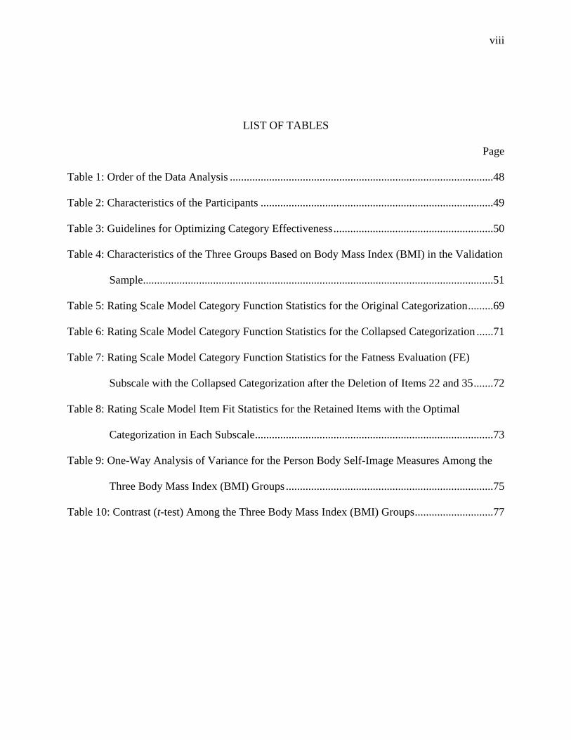
LIST OF TABLES

Page

Table 1: Order of the Data Analysis ..............................................................................................48

Table 2: Characteristics of the Participants ...................................................................................49

Table 3: Guidelines for Optimizing Category Effectiveness.........................................................50

Table 4: Characteristics of the Three Groups Based on Body Mass Index (BMI) in the Validation

Sample.............................................................................................................................51

Table 5: Rating Scale Model Category Function Statistics for the Original Categorization.........69

Table 6: Rating Scale Model Category Function Statistics for the Collapsed Categorization ......71

Table 7: Rating Scale Model Category Function Statistics for the Fatness Evaluation (FE)

Subscale with the Collapsed Categorization after the Deletion of Items 22 and 35.......72

Table 8: Rating Scale Model Item Fit Statistics for the Retained Items with the Optimal

Categorization in Each Subscale.....................................................................................73

Table 9: One-Way Analysis of Variance for the Person Body Self-Image Measures Among the

Three Body Mass Index (BMI) Groups ..........................................................................75

Table 10: Contrast (t-test) Among the Three Body Mass Index (BMI) Groups............................77

ix

LIST OF FIGURES

Page

Figure 1: Rating scale model category probability curves for the original and collapsed

categorizations for the social dependence (SD) subscale..............................................79


categorizations for the height dissatisfaction (HD) subscale ........................................80


categorizations for the investment in ideals (II) subscale .............................................81


categorizations for the fatness evaluation (FE) subscale after the deletion of the items

22 and 35 .......................................................................................................................82

Figure 5: Map for the person and item parameter estimates for the overall appearance evaluation

(OAE) subscale..............................................................................................................83

Figure 6: Map for the person and item parameter estimates for the fatness evaluation (FE)

subscale .........................................................................................................................84

Figure 7: Map for the person and item parameter estimates for the attention to grooming (AG)

subscale .........................................................................................................................85

Figure 8: Map for the person and item parameter estimates for the health fitness evaluation

(HFE) subscale ..............................................................................................................86

Figure 9: Map for the person and item parameter estimates for the health fitness influence (HFI)

subscale .........................................................................................................................87

x

Figure 10: Map for the person and item parameter estimates for the social dependence (SD)

subscale .........................................................................................................................88

Figure 11: Map for the person and item parameter estimates for the height dissatisfaction (HD)

subscale .........................................................................................................................89

Figure 12: Map for the person and item parameter estimates for the negative affect (NA)

subscale .........................................................................................................................90

Figure 13: Map for the person and item parameter estimates for the investment in ideals (II)

subscale .........................................................................................................................91

Figure 14: Differential item functioning of the Body Self-Image Questionnaire (BSIQ) in the

total sample and the validation sample..........................................................................92

Figure 15: Curvilinear relationship between the raw scores and the Rasch calibrated person

measures for the Overall Appearance Evaluation (OAE) subscale...............................93

1

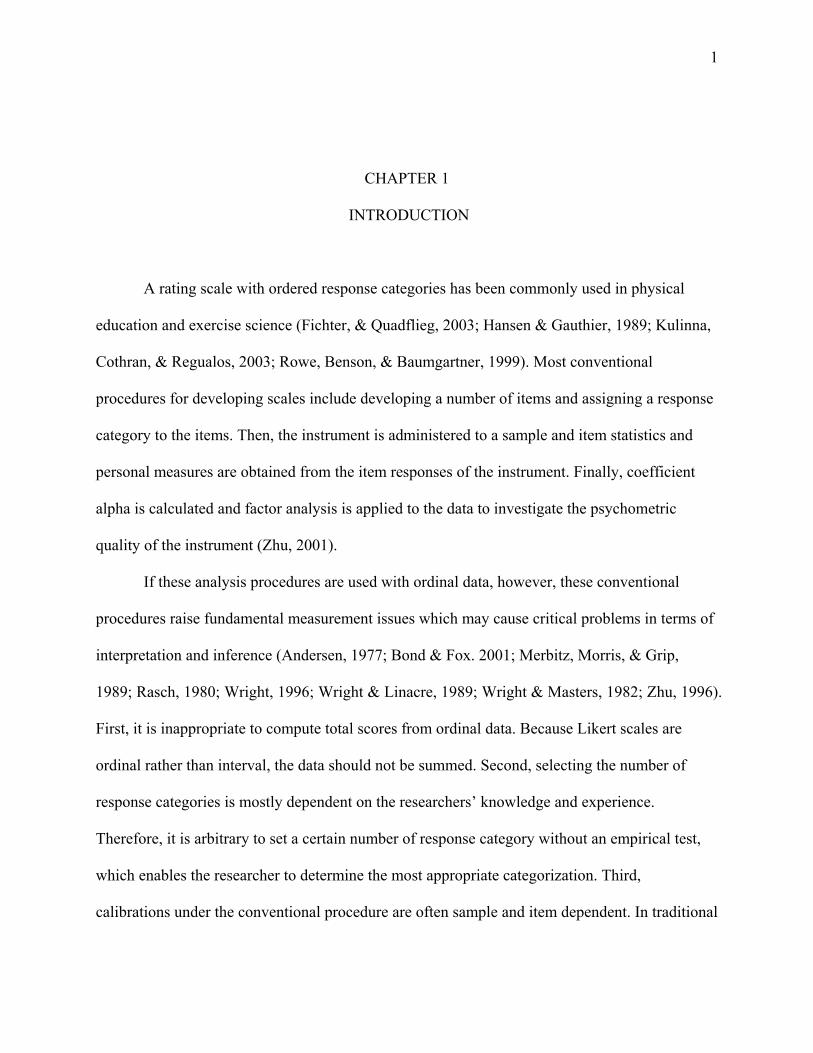
CHAPTER 1

INTRODUCTION

A rating scale with ordered response categories has been commonly used in physical

education and exercise science (Fichter, & Quadflieg, 2003; Hansen & Gauthier, 1989; Kulinna,

Cothran, & Regualos, 2003; Rowe, Benson, & Baumgartner, 1999). Most conventional

procedures for developing scales include developing a number of items and assigning a response

category to the items. Then, the instrument is administered to a sample and item statistics and

personal measures are obtained from the item responses of the instrument. Finally, coefficient

alpha is calculated and factor analysis is applied to the data to investigate the psychometric

quality of the instrument (Zhu, 2001).

If these analysis procedures are used with ordinal data, however, these conventional

procedures raise fundamental measurement issues which may cause critical problems in terms of

interpretation and inference (Andersen, 1977; Bond & Fox. 2001; Merbitz, Morris, & Grip,

1989; Rasch, 1980; Wright, 1996; Wright & Linacre, 1989; Wright & Masters, 1982; Zhu, 1996).

First, it is inappropriate to compute total scores from ordinal data. Because Likert scales are

ordinal rather than interval, the data should not be summed. Second, selecting the number of

response categories is mostly dependent on the researchers’ knowledge and experience.

Therefore, it is arbitrary to set a certain number of response category without an empirical test,

which enables the researcher to determine the most appropriate categorization. Third,

calibrations under the conventional procedure are often sample and item dependent. In traditional

2

item analysis, item difficulty is estimated based on the proportion of correct responses in a

sample, and item discrimination is represented by the correlation between item scores and total

test scores. Person ability also depends on the particular collection of items used in an instrument.

Therefore, levels of item difficulty and person ability may change based on the characteristics of

samples (i.e., the level of ability and homogeneity of a sample being tested). These dependencies

make it difficult to have consistent research findings and to compare findings across studies with

various samples. Last, items and respondents are calibrated on different scales in conventional

procedures. For example, means and standard deviations of items are used for item investigation

and total scores are used for respondents’ summaries. Therefore, both facets, item difficulty and

person ability, cannot be compared on the same metric.

Similar issues have been debated in fields such as psychology, education, and medical

rehabilitation (e.g., Andrich, 1978; Merbitz, Morris, & Grip, 1989; Wright, 1996; Wright &

Linacre, 1989), and many researchers have applied the Rasch analysis to ordinal data to solve

these problems (Kirby, Swuste, Dupuis, MacLeod, & Monroe, 2002; Waugh, 2003). Originally,

the Rasch model was developed for dichotomously scored items to construct objective measures

that enable a researcher to define the difficulty of an item and the ability of an individual

independent from population and items, respectively (Rasch, 1960/1980). Even though the Rasch

model is also known as a one-parameter logistic model of item response theory (IRT), the early

studies of the Rasch model were not closely related to IRT and Rasch barely referred to IRT

literature in his studies. Rather, some researchers approached the Rasch model with IRT

concepts. Andersen (1973) approached the Rasch model with conditional maximum likelihood

estimation (MLE) procedures, and Masters and Wright (1984) described five Rasch families of

latent trait models within the IRT framework. Further, Andrich (1978) extended the idea of the

3

Rasch modeling to a rating scale model in which items with ordered response categories can be

analyzed.

From the various applications of the Rasch model to rating scales, several advantages of

the Rasch analysis have been defined. First, the Rasch model provides a simple and practical

way to construct linear measures from any ordered nominal data so that subsequent statistical

analysis can be applied without a concern for linearity. Second, parameter estimations are

independent from the individuals and items used. Third, testing results can be interpreted in a

single reference framework because both item difficulty and individual ability are located on the

same scale. Due to these features, it has been reported that the application of the Rasch model is

advantageous to construct objective and additive scales (Bond & Fox, 2001).

In physical education and exercise science, some researchers have applied the Rasch

model to rating scales for calibrating and optimal categorizing of instruments, and developing

objective measures (Kulinna & Zhu, 2001; Looney, 1997; Looney & Rimmer, 2003; Zhu & Cole,

1996; Zhu & Kurz, 1994; Zhu, Timm, & Ainsworth, 2001). Although the advantages of the

Rasch analysis have been introduced, it has not been widely used in the field because treating

raw scores as interval measures sometimes seems to work due to the carefully designed interval-

like response categories and the monotonous relationship between scores and measures in special

situations. However, these cases are rare in practice and empirically not proven, so it is still

preferable to convert raw scores to linear measures.

The interest in body image has increased as dissatisfaction with body image has been

considered a contributory factor in the development of eating disorders (Smolak, 2002). A

variety of instruments have been developed to measure the construct of body image. However,

Rowe (1996) pointed out two problems with existing body image instruments. First, despite the

4

large number of instruments available, few were developed using rigorous methods such as

investigating construct validity evidence. Second, even though some instruments were developed

for measuring body image, they are measuring different constructs of body image or the term

‘body image’ is being used in different ways in those studies. For this reason, Rowe (1996)

developed a scale, the Body Self-Image Questionnaire (BSIQ), for measuring the body image

construct in a more comprehensive and systematic way.

Although the BSIQ was developed through four stages of elaborate investigations such as

collecting items from a review of the literature and current instruments, revising items using

exploratory factor analysis, defining factors and items using confirmatory factor analysis, and

investigating construct validity, the fundamental measurement problems still exist in analyzing

data from this ordinal scale. Therefore, applying the Rasch model to the BSIQ is necessary to

provide a solution for current measurement concerns, such as linear measures and optimal

categorization, and to define body image items and individual scores on the same metric.

Statement of Problem

Even though ordinal data are not sufficiently interval to justify researchers to do

arithmetic calculations on the data, it is common in practice to analyze ordinal data as though

they are interval measures. A measurement model that provides a way to construct linear

measures from ordinal data has been introduced and extended for various applications since the

1960s and currently many computer programs are available for application of the model to rating

scales. However, only a few studies have been done using the Rasch models in the physical

education and exercise science fields and the measurement model has not been employed in

developing and investigating body image scales.

5

The BSIQ consists of 39 items and a Likert-type 5-point response scale for each item.

Even though validity of the BSIQ was investigated with various statistical techniques, the

linearity of measures and the function of categorization have not been investigated. Therefore, it

was required to transform the ordinal data to logits using IRT for analyzing subscale scores or

conducting any further statistical analysis. Additionally, it was necessary to exam the

categorization as to whether each response category would function as intended because optimal

categorization was known to improve the quality of measurement.

Purpose of Study

The primary purpose of this study was to calibrate the BSIQ by transforming ordinal data

into logits for investigating both item difficulty and person ability on the same continuum. The

secondary purpose was to examine the categorization of each subscale of the BSIQ and to

determine the optimal categorization for the subscales with problematic categorization. Through

the Rasch analysis, it was expected that the Rasch analysis would provide an effective

framework describing the nature of body image items and respondents’ attribute on the same

metric and improve the function of rating scale categorization.

Research Questions

During this study, the following research questions were addressed.

1. Will the data of the BSIQ fit the model in terms of Infit and Outfit?

2. Will the Rasch model calibration adequately contrast items and participants in terms of

item difficulty and the level of the attribute?

3. Is the response categorization of the BSIQ functioning as intended in terms of

frequencies, average measures, step calibrations, and Outfit statistic? When any violation

or misfitting is found in category function, will the collapsing procedure solve the

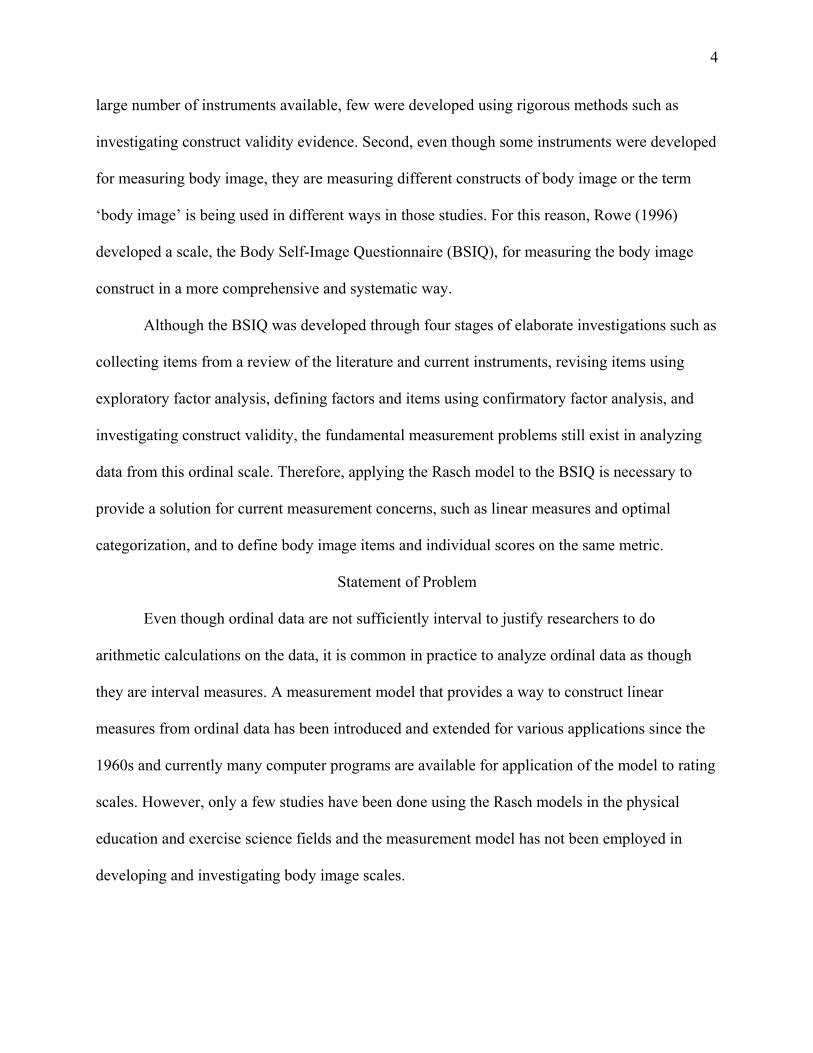
6

problem of the categorization? And which pattern of collapsing combinations is most

appropriate to each subscale of the BSIQ?

4. Will the Rasch calibrated item and person parameters and the revised categorization be

stable when a smaller sample is calibrated?

Delimitations of the Study

1. Data from a previous study were used for this study. The data were collected from

undergraduate students with ages 17 to 25. The students were participating in at least one

of basic physical education activity classes.

2. The rating scale model was used in the present study with the assumption that the effect

of guessing was minimal and the item discrimination was identical across the items.

3. In collapsing procedure, the linguistic aspects of category definitions such as word

clarity, substantive relevance, and conceptual sequence, were assumed to be plausible.

So, only numerical and empirical aspects of categorization such as hierarchical order of

average measures, step advance, and category fit statistics were considered in

determining optimal categorization.

Definition of Terms

Calibration. Traditionally, it refers to a process of translating scores obtained from

several tests of different difficulty levels to a single common score scale (Chang, 1985). Scaling

is an interchangeable term indicating the development of systematic rules and meaningful units

of measurement for quantifying empirical observations (Crocker & Algina, 1986). In the Rasch

analysis, calibration refers to a process of converting raw scores to logits to determine the values

of item difficulty and person ability in a metric for the underlying latent trait.

7

Rating scale model. It is one of the Rasch family of models developed by David

Andrich (1978). The rating scale model can be applied to polytomous data obtained from ordinal

scales or Likert scales. In the item response theory framework, the rating scale model is

categorized as a one-parameter logistic model.

Optimal Categorization. In the Rasch analysis, the term optimal is relative to the

original categorization for an instrument rather than the best categorization. Therefore, the

optimal categorization refers to a categorization which produces the hierarchical order in average

measures and step calibrations, and better fit statistics and separation statistics than other

combinations of categorization.

Fundamental measurement. It refers to the idea that requires an ordering system and the

characteristics of additivity in assigning numbers to objects to represent their properties. The

Rasch model is a type of additive conjoint measurement which satisfies these requirements of

fundamental measurement.

Linearity. It refers to the idea or the characteristics of measurement which is additive

such as length and weight. In the Rasch analysis, the qualitative variations of the raw scores are

transformed into logits on a linear scale to have the characteristics of linear measure.

Invariance. This term indicates the maintenance of the identity of a variable from one

occasion to the next. In theory, the process of measurement can be repeated without modification

in different parts of the measurement continuum due to the two dominant advantages of the

Rasch model which provides sample–free item calibration and test-free person measurement. For

example, if two item difficulty estimates obtained from different groups for any particular item

are transformed and placed on a common metric, the two item difficulty estimates should have

approximately the same values.

8

Latent trait. This term refers to certain human attributes that are not directly

measurable. In the theory of latent model, a person’s performance can be quantified and the

values are used to interpret and explain the person’s test response behavior. Frequently, trait and

ability are used interchangeably in the literature.

Logit. The abbreviation of log odds unit. The unit of measurement that results when the

Rasch model is used to transform raw scores obtained from ordinal data to log odds ratios on a

common interval scale. A logit has the same characteristics of an interval scale in that the unit of

measurement maintains equal differences between values regardless of location. The value of 0.0

logit is routinely allocated to the mean of the item difficulty estimates (Bond & Fox, 2001).

Probabilistic. Given that all the possible influences on a person’s performance cannot be

known, the outcomes of the Rasch model are expressed mathematically as probabilities. For

example, the Rasch measurement is probabilistic; the total score predicts with varying degrees of

certainty which items were correctly answered.

9

CHAPTER 2

RELATED RESEARCH

The primary purpose of this study was to calibrate the BSIQ (Rowe, 1996) by

transforming the raw data from an ordinal scale into logits for investigating both item difficulty

and person ability (i.e., body image satisfaction) on the same continuum. The secondary purpose

was to determine the optimal categorization of the BSIQ. Presented in this chapter are an

overview of rating scales, the Rasch models, the Rasch model assessment, the Rasch calibration,

optimal categorization, and measurement of body image.

Overview of Rating Scales

Rating scales with response options are designed to extract more information out of an

item than information obtained from an item with a dichotomous scale. A rating scale with

response options is classified as an ordinal scale based on Stevens’ (1946) classification system.

Likert scales have been the dominant type of categorizations in rating scales to collect attitude

data. A Likert scale was originally expressed with five possible response options; strongly

disagree, disagree, neutral, agree, and strongly agree. In general, each item is presented to a

participant with a statement and a five-point scale. Then, the participant is asked to choose a

response from the five-point scale. This ordinal scale does not provide either a common unit of

measurement between scores or the origin that indicates absolute zero but provides only an order

between scores (Baumgartner, Jackson, Mahar, & Rowe, 2003). Due to the absence of equal

10

measurement units and unknown distance between scores, responses in an ordinal scale should

not be added for obtaining total or subscale scores.

Problems in Analyzing Ordinal Data

Many instruments and questionnaires assessing attitude have used on rating scales and

the number of studies using a rating scale is increasing as new instruments and questionnaires are

being developed. The procedures for developing rating scales have been well introduced in many

studies in order to develop a sound understanding of complex models and theories (Benson &

Nasser, 1998; Crocker, Llabre, & Miller, 1988; Dunbar, Koretz, & Hoover, 1991; Ennis &

Hooper, 1988; Klockars & Yamagishi, 1988). However, the appropriate procedures for analyzing

rating scales with ordinal scales have not been well introduced and the procedures have been

ignored. As a result, ordinal integer labels (e.g., strongly agree = 5) from rating scales are

commonly analyzed as though they were interval measures and means and total scores are

calculated.

According to Bond and Fox (2001), measures must be objective abstractions of equal

units to be reproducible and additive. If total scores are obtained from a scale without meaningful

order or equal measurement units, they will not be meaningful for tests and analyses. Because

order and equal distance between score units are critical features of addition and subtraction, a

rating scale which has only one feature is not summative. Indeed, total scores are the sums of all

responses in the scales, which are ordinal, so analyzing total scores is not appropriate. Thus,

misuses of means and total scores generated from ordinal scales are often misleading. Stevens

(1946) suggested that the statistics involving means and standard deviations should not be used

with ordinal scales because the ordinal scale arises from the operation of rank-ordering

procedure. In other word, although 4 is greater than 3 and 2 is greater than 1 in terms of the level

11

of the trait being measured, the sum of 4 and 1 may not necessarily be equal to the sum of 3 and

2 because the difference between 1 and 2 may not be identical to the difference between 3 and 4

due to the absence of the linearity of measures. Crocker and Algina (1986) also suggested that

total score from a scale without meaningful order and equal measurement units cause confusion

when it is used for determining validity or reliability of an instrument because it is virtually

impossible to detect whether a problem (e.g., low coefficient) is caused by inappropriate numeric

properties or inadequate validity or reliability of the instrument.

The ideas of fundamental measurement started being raised by some researchers in the

early 1900s. Thorndike (1926) indicated the need for an equal-interval scale in which one step

increment of integer labels would represent amounts increasing by a constant difference.

Thurstone (1925, 1927) suggested using an absolute scale that approximates an equal-interval

scale, even though it was pointed out that the absolute scale lacked objectivity due to the

dependency on the ability distribution of participants (Wright & Stone, 1979). Later, the need for

objective measurement, which is independent of the original scale and of the original group

tested has been advocated by many researchers (Gulliksen, 1950; Loevinger, 1947) and which

does not change with the times so that an accumulation of data for historical comparisons is

accessible (Angoff, 1960).

To summarize, items using rating scales are requiring participants’ opinions to which

numbers are arbitrarily assigned to response categories to produce ordinal data. Therefore,

ordinal data are not sufficiently interval to justify the arithmetical calculations used for obtaining

means and variances (Wright, 1996). To satisfy the requirements for the analysis of ordinal data,

transformed measures rather than raw data are needed for the analysis.

12

Problems in Developing Rating Scale Categorization

Determination of the well-functioning categorization has been an issue of interest to scale

developers and many researchers have attempted to provide the optimal categorization in terms

of the number of categories and the type of anchors (e.g., Guilford, 1954; Parducci & Wedell,

1986; Wedell, Parducci, & Lane, 1990). Since Likert introduced a five category agreement scale

in 1932, there have been many arguments that eliminating the neutral category increases the

quality of a scale, using more response categories rather than fewer categories is more

advantageous, and a large number of response categories may confuse examinees (e.g., Guilford,

1954). Although the best method for constructing categorization has not been provided, it is

commonly known that the way each rating scale is constructed is directly related to the way the

variable is divided into categories, which affects the measurement quality of the data obtained

from the scale (Clark & Schober, 1992; Linacre, 2002). Several features are required for an

optimal categorization to elicit unambiguous responses. First, rating scales should reflect a

common construct or trait in each question. Second, each category should have a respective

boundary and those boundaries should be ordered based on the change of magnitudes of the trait

(Guilford, 1954).

In the past, merely counting frequencies in each category has been the only method to

investigate rating scale categorization. Some other statistics are also employed to test the scale

and items, but none of these traditional statistics are appropriate for investigating the quality of

categorization. For example, coefficient alpha and item-total correlation are used for determining

homogeneity of the scale and items. However, it is still not clear whether the categories are

systematically ordered because these statistics do not provide statistical information about the

categorization being used. For this reason, only the number of items and the quality of each item

13

are overviewed based on the results of conventional statistics. Consequently, determining the

number of response categories mostly relies on the researchers’ knowledge or previous studies.

Even with great effort to develop an unambiguous rating scale, however, a test developer

may fail to have participants react to a rating scale as designed (Roberts, 1994; Zhu, 2002).

Applying only abstractive ideas and subjective knowledge to developing the optimal number of

category has limitations in that no empirical test results are provided and the characteristics of

the category function is not known.

Analyzing a Rating Scale

Traditionally, counting frequencies and transforming raw data have been employed to

analyze a rating scale. Even though counting frequencies is somewhat simple and

straightforward, applying this procedure is very limited in practice because analysis beyond each

participant’s ability is not available (Zhu, 1996). Transforming procedure, also known as

mathematical models, can be classified in two ways: deterministic and probabilistic models. To

obtain measurements from discrete observations, it is necessary to transform the observations

from a rating scale to an interval or ratio scale before conducting an analysis.

Deterministic models

A deterministic model provides an exact prediction of an outcome based on assumptions

such as no unsystematic or error variance in the model and all interpretable variation in the

response is produced by the respondents and items. For example, a response pattern required by

a Guttman scale shows perfect variation such as ‘1-1-1-1-1-1-0-0-0-0-0’, where ‘1’ indicates

correctly answered items and ‘0’ refers to incorrectly answered items.

However, Guttman model expectations for step-like development of sequential skills are

unrealistically strict. In this model, each person must respond correctly to items in order of

14

difficulty until the difficulty of an item exceeds a person’s ability. Then the person must respond

incorrectly to all other items that are more difficult. Therefore, unexpected responses caused by

participants guessing or fatigue commonly observed in practice, are not allowed in the model.

According to Andrich (1988), an error may exist between the prediction and the real

value under the deterministic model, in which the error does not count because the values of

interest are sufficiently great relative to the error, so the error would be ignored. In a

deterministic procedure, participants are asked to rate each item in a number of categories

previously defined. Based on the ratings, the values of the categories on an underlying

continuum can be estimated and interval-scale values of the item can be determined (Zhu, 1996).

Therefore, the deterministic model is used only for scaling items rather than individuals. The

limitations of this model are that applying deterministic models is arbitrary because goodness-of-

fit is not available in the model, and that deterministic models cannot account for variation in

participants’ responses to items due to the separate relation of each participant and each item to

the underlying variable (Togerson, 1958). Furthermore, the deterministic models are likely to fit

only a few types of data due to its empirically unrealistic expectations.

Probabilistic Models

In contrast to the deterministic approach, a probabilistic model assumes that there is a

certain amount of unsystematic variance in the model. Therefore, the model may or may not

account for all of the relevant causes of the outcome, and replications may produce differences in

outcomes (Andrich, 1988). As a result, the outcomes are formalized in terms of probabilities.

This probabilistic feature is more realistic in empirical practice. Indeed, the probabilistic model

provides statistical criteria for goodness-of-fit of the model to the data which are advantageous

for determining acceptance or rejection of a scaling hypothesis (Togerson, 1958).

15

The early work on probabilistic models mostly utilizes dichotomous data. Those models

include the latent-linear model (Lazarsfeld & Henry, 1968), the latent distance model (Lazarsfeld

& Henry, 1968), the normal ogive model (Lord, 1952), and logistic ogive models (Birnbaum,

1968). Lord’s work on the normal ogive models in the 1950s was recognized as the origin of IRT.

The normal ogive models were not easy to use due to their complex mathematical procedures

such as integration. Later, Birnbaum introduced the logistic models and their statistical

foundations as the form of the item characteristic curve, which is an explicit function of item and

ability parameters. The logistic models were substituted for the normal ogive models so the

normal ogive models are used mainly for historic reasons such as the relationship to classical test

theory (Embretson & Reise, 2000; Zhu, 1990). All estimates in the logistic model essentially

have the same interpretation as in the normal ogive model only if a scaling factor D (1.702) is

added to the equation (Haley, 1952). The Rasch model, which is categorized to the logistic

models, incorporates the attractive ordering features of the Guttman’ scale model and

complements them with a more realistic probabilistic, stochastic framework (Bond & Fox, 2001).

The Rasch Models

The Rasch model was developed under the probabilistic concepts. As a result of interest

in modeling the relationship between a participant’s underlying ability and response to a testing

item, Rasch (1960/1980) constructed objective measures using dichotomously scored

intelligence test scores to define item difficulty independent of participants being tested and

person ability independent of test items being provided. Person ability is described as a position

on an ability metric (i.e., latent continuum) and item difficulty is represented as the point on the

ability metric at which the person has a fifty percent chance of answering the item correctly

(Chang, 1985). Because the person ability and the item difficulty govern the probability of any

16

participant being successful on any particular item, the probability is a function of these two

measures. In other word, the model expresses the probability of obtaining a correct answer as a

function of the size of the difference between the ability of the person and the difficulty of the

item. For example, a person has a higher probability of correctly answering an item that has

lower difficulty than the ability of the person, and a lower probability of correctly answering an

item with higher difficulty than the ability of the person. Although it is a simple concept, it is a

critical feature of the Rasch model.

Even though the Rasch model was developed independently within the framework of

probabilistic approach, the Rasch model is classified as an item response model in which the

item characteristic curve is a one-parameter logistic function (Hambleton, 1985). Since the Rasch

analysis was introduced, it has been extended to several models by researchers (e.g., Andersen,

1973; Andrich, 1978; Master, 1982; Master & Wright, 1984).

Logistic Models

The Rasch model is a simple stochastic model originally devised for dichotomously

scored items. The Rasch model is categorized as a one-parameter logistic model of IRT (Zhu,

1990). In IRT an item characteristic curve (ICC) plays an important role. The ICC is the S-

shaped curve indicating the relationship between the probability of correct response to an item

and the ability scale (Baker, 1992). The ICC can be obtained from several mathematical models

which are cumulative forms of the logistic function. One-, two-, and three-parameter logistic

models are standard mathematical models and the most commonly known IRT models. While all

three models are commonly utilizing dichotomous scores and employing an ability parameter

and an item difficulty parameter, different numbers of parameter(s) are employed in each model.

17

Therefore, each model may result in different results with the same data. The mathematical

forms of the three logistic models are defined as,

( )

( )( )1

i

i

b

i beP

e

θ

θθ−

−=+

, (one-parameter model) (2.1)

( )

( )( )1

i i

i i

a b

i a beP

e

θ

θθ−

−=+

, (two-parameter model) (2.2)

( )

( )( ) (1 )1

i i

i i

a b

i i i a beP c c

e

θ

θθ−

−= + −+

. (three-parameter model) (2.3)

where Pi(θ ) = the probability that a randomly selected examinee with ability θ will answer item

i correctly,

a = the discrimination parameter of item i,

b = the difficulty parameter of item i,

c = the pseudo-guessing parameter (the probability of guessing), and

e = an exponent of the natural constant which equals 2.71828.

A one-parameter model involves an item parameter b denoting difficulty of a test item and an

ability parameter θ indicating ability level of a participant. It is known as a one-parameter

model because only one item parameter is designated in this model. A one-parameter model is

similar to a three-parameter model if the pseudo-guessing parameter c is assumed to be minimal

and the item discrimination a is assumed to be the same across all items in the test. Birnbaum

proposed the two-parameter logistic model to substitute for the two-parameter normal ogiv

model (Hambleton, 1985). The difference between a three-parameter model and a two-parameter

model is that in a two-parameter model there is no pseudo-guessing factor involved. The form of

the ICC of this model is determined by the difficulty parameter b and the discrimination

parameter a. The discrimination parameter dependent on the item information reflects the

e

18

steepness of the form of the ICC. The three-parameter logistic model differs from the two-

parameter model in that the pseudo-guessing parameter is involved. The two-parameter log

model can be obtained from the three-parameter logistic model mathematically if the pseu

guessing parameter is assumed to be zero. The parameter c describes the goodness-of-fit of

low asymptote of the ICC and represents the probability of participants with low ability correc

answering an item by guessing. Among the three logistic models, the one-parameter logistic

model is easier to apply and the model produces less estimation problems than other logistic

models because a fewer number of item parameters is employed in the model.

istic

do-

the

tly

Rasch Dichotomous Model

The Rasch dichotomous model is the original and simplest form of the Rasch family of

models, which utilizes dichotomous scores such as correct and incorrect, yes and no, or present

and absent. The Rasch dichotomous model is also classified as a one-parameter logistic model

because the model predicts probabilities using an exponential form and includes one item

parameter in describing items (Embretson & Hershberger, 1999). In a testing situation, score 1 is

given to correct answer while 0 is assigned to incorrect response because there are only two

response categories.

The Rasch dichotomous model uses the total score for estimating probabilities of

response. Estimation of item difficulty and person ability starts from calculating the percentage

of correct responses. For the estimation of person ability, the ratio of the percentage correct over

the percentage incorrect calculated from each respondent is converted into odds. For example,

when a person has completed four questions correct and six questions incorrect in a test with

total of 10 questions, the ratio for the person is 40/60 and the natural log of the ratio is calculated.

The value of ln(40/60) is assigned to the person for his or her ability estimate (-.4). For the

19

estimation of item difficulty, the same calculation is applied. These transformed values for items

and persons are scaled on the same metric which is called logits. During the series of iteration for

estimating parameter measures, the person ability estimates are constraint when item difficulties

are estimated and vice versa. Therefore, estimations of difficulty parameter and ability parameter

are statistically independent from testing items and samples used in the Rasch calibration. This

invariance feature is the core of the Rasch analysis and also plays a important role in interpreting

test results. Finally, the difference between the person parameter estimates (i.e., ability) and the

item parameter estimates (i.e., difficulty) can be used to obtain the probabilities of success. This

whole process of calculation transforms ordinal-level data into logits which have the same

characteristics of interval data.

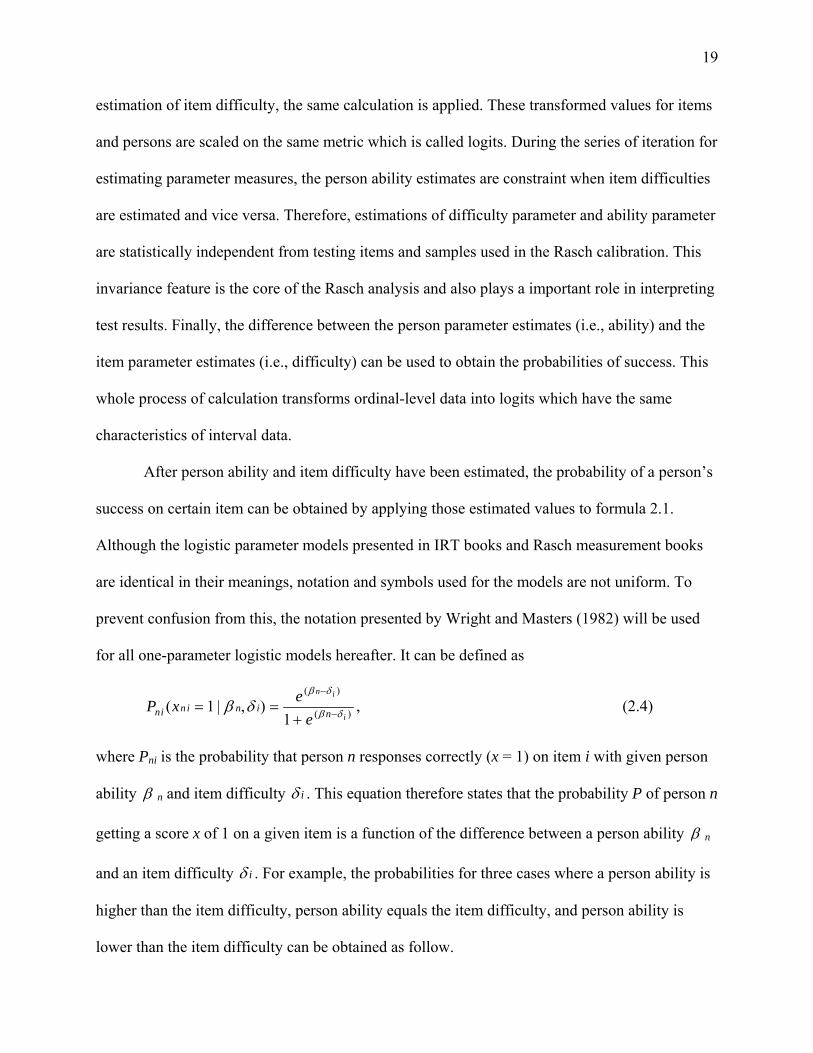
After person ability and item difficulty have been estimated, the probability of a person’s

success on certain item can be obtained by applying those estimated values to formula 2.1.

Although the logistic parameter models presented in IRT books and Rasch measurement books

are identical in their meanings, notation and symbols used for the models are not uniform. To

prevent confusion from this, the notation presented by Wright and Masters (1982) will be used

for all one-parameter logistic models hereafter. It can be defined as

( )

(( 1 | , )1

n i

in i n ini n

eP xe

β δ

)β δβ δ−

−= =+

, (2.4)

where Pni is the probability that person n responses correctly (x = 1) on item i with given person

ability β n and item difficulty iδ . This equation therefore states that the probability P of person n

getting a score x of 1 on a given item is a function of the difference between a person ability

β n

and an item difficulty iδ . For example, the probabilities for three cases where a person abilit

higher than the item difficulty, person ability equals the item difficulty, and person ability is

lower than the item difficulty can be obtained as follow.

y is

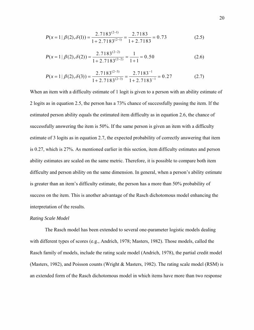
20

(2 1)

(2 1)2.7183 2.7183( 1 | (2), (1)) 0.7

1 2.71831 2.7183P x β δ

−

−= = =++

3= (2.5)

(2 2)

(2 2)2.7183 1( 1 | (2), (2)) 0.50

1 11 2.7183P x β δ

−

−= = =++

= (2.6)

(2 3) 1

(2 3) 12.7183 2.7183( 1 | (2), (3)) 0.2

1 2.7183 1 2.7183P x β δ

− −

− −= = =+ +

7= (2.7)

When an item with a difficulty estimate of 1 logit is given to a person with an ability estimate of

2 logits as in equation 2.5, the person has a 73% chance of successfully passing the item. If the

estimated person ability equals the estimated item difficulty as in equation 2.6, the chance of

successfully answering the item is 50%. If the same person is given an item with a difficulty

estimate of 3 logits as in equation 2.7, the expected probability of correctly answering that item

is 0.27, which is 27%. As mentioned earlier in this section, item difficulty estimates and person

ability estimates are scaled on the same metric. Therefore, it is possible to compare both item

difficulty and person ability on the same dimension. In general, when a person’s ability estimate

is greater than an item’s difficulty estimate, the person has a more than 50% probability of

success on the item. This is another advantage of the Rasch dichotomous model enhancing the

interpretation of the results.

Rating Scale Model

The Rasch model has been extended to several one-parameter logistic models dealing

with different types of scores (e.g., Andrich, 1978; Masters, 1982). Those models, called the

Rasch family of models, include the rating scale model (Andrich, 1978), the partial credit model

(Masters, 1982), and Poisson counts (Wright & Masters, 1982). The rating scale model (RSM) is

an extended form of the Rasch dichotomous model in which items have more than two response

21

categories with order (e.g., Likert scales). An item with five response categories is modeled as

having four thresholds. For example,

Strongly Strongly

Disagree Disagree Neutral Agree Agree

0 1st 2nd 3rd 4th

if a participant chooses “Agree” for an item on an attitude questionnaire, the participant can be

considered to have chosen “Disagree” over “Strongly Disagree”, “Neutral” over “Disagree”, and

also “Agree” over “Neutral”, but to have failed to choose “Strongly Agree” over “Agree”.

Therefore, completing the kth step can be thought of as choosing the kth alternative over the (k-

1)th alternative in response to the item. Then the participant scores 3 on the item because the

third step has been taken.

The RSM is distinguished from the Rasch dichotomous model by the threshold parameter

kτ . This new added parameter is a set of estimates for the certain number of thresholds that

indicate the boundaries on the continuum between response categories (Andrich, 1978; Wright &

Masters, 1982). The thresholds are estimated once for all items so, the set of threshold values are

applied identically to all of the items on the scale. Therefore, the thresholds are the same across

items in the same scale because it is assumed that items differ only in their locations, but not in

their corresponding response categories, and the same set of alternatives is used with every item

(Andersen, 1977; Andrich, 1978). The step difficulties are derived from the estimated item

difficulties and thresholds. Each step difficulty is the sum of the item difficulty and each step

threshold. Then the item difficulty is the mean of the step difficulties (Zhu, 1996). This

expectation can be expressed by resolving each item difficulty from equation 2.4 into two

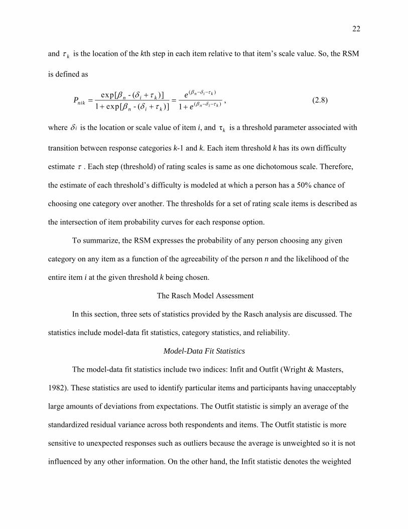
components so ik i kδ δ τ= + , where iδ is the location or scale value of item i on the variable

22

and kτ is the location of the kth step in each item relative to that item’s scale value. So, the RSM

is defined as

( )

(exp[ - ( )]

1 exp[ - ( )] 1

n i k

n i k

n i knik

n i k

ePe

β δ τ

β δ τβ δ τβ δ τ

− −

− −

+= =

+ + + ) , (2.8)

where iδ is the location or scale value of item i, and is a threshold parameter associated with

transition between response categories k-1 and k. Each item threshold k has its own difficulty

estimate

τk

τ . Each step (threshold) of rating scales is same as one dichotomous scale. Therefore,

the estimate of each threshold’s difficulty is modeled at which a person has a 50% chance of

choosing one category over another. The thresholds for a set of rating scale items is described as

the intersection of item probability curves for each response option.

To summarize, the RSM expresses the probability of any person choosing any given

category on any item as a function of the agreeability of the person n and the likelihood of the

entire item i at the given threshold k being chosen.

The Rasch Model Assessment

In this section, three sets of statistics provided by the Rasch analysis are discussed. The

statistics include model-data fit statistics, category statistics, and reliability.

Model-Data Fit Statistics

The model-data fit statistics include two indices: Infit and Outfit (Wright & Masters,

1982). These statistics are used to identify particular items and participants having unacceptably

large amounts of deviations from expectations. The Outfit statistic is simply an average of the

standardized residual variance across both respondents and items. The Outfit statistic is more

sensitive to unexpected responses such as outliers because the average is unweighted so it is not

influenced by any other information. On the other hand, the Infit statistic denotes the weighted

23

mean square which has more emphasis on unexpected responses near a person’s measure or an

item’s measure. Both Outfit and Infit statistics having values near 1 are considered satisfactory

indications of model-data fit, and significantly larger or smaller values are considered misfit. A

larger value indicates inconsistent performance, while a smaller value reflects too little variation.

The estimation of fit begins with the calculation of a response residual for each

respondent when each item is encountered. Response residual is the deviation of the actual

response from the Rasch model expectations. The Rasch analysis provides an expected value of

the response nix for each person-item encounter in the data matrix. This expected value falls

between 0 and the number of steps (thresholds), and is given by

0

m

ni nikk

E kP=

= ∑ , (2.9)

where is person n’s modeled probability of responding in category k to item i. When the

expected value

nikP

niE is subtracted from the observed response nix , a score residual is obtained

as following

niy

ni ni niy x E= − . (2.10)

Score residuals can be calculated in this way for every cell of the data matrix. When data fit the

RSM each score residual has an expected value of zero. To evaluate the score residual and i

square 2niy e compute the variance of ni

niy ts

w x by

P

P

2

0( )

m

ni ni nikk

W k E=

= −∑ (2.11)

and its kurtosis by

4

0( )

m

ni ni nikk

C k E=

= −∑ . (2.12)

24

The variance is largest when the person and item estimates are identical and decreases as

person n and item i become further apart. As is also the variance of score residual , this

score residual can be standardized by

niW

niW niy

1/ 2ni ni ni

nini ni

x E yzW W−

= = . (2.13)

These estimated values , , and niW niC niz are applied to the estimations of Outfit, Infit, and t-

values.

Estimation of item fit. Because there are too many deviations, or residuals to examine in

one matrix, the fit diagnosis typically is summarized in a fit statistic. One approach to

summarizing the fit of an item to a measurement model is to square each of the standardized

residuals for that item and average these squared residuals over the N persons. An unweighted

mean square, called Outfit, can be calculated as

2

1

N

nin

i

Zu

N==∑

. (2.14)

A disadvantage of statistic is that it is rather sensitive to unexpected responses made by

persons for whom item i is far too easy or far too difficult. When is used, we may be led to

reject an item as misfit because of just two or three unexpected responses made by persons for

whom the item was quite inappropriate. An alternative is to weight the squared residuals so that

responses made by persons for whom the item is inappropriate have less influence on the

magnitude of the item fit statistic. A weighted mean square, called Infit, can be calculated as

iu

iu

2 2

1

1 1

N N

ni ni nin ni N N

ni nin n

1Z W y

vW W

= =

= =

= =∑ ∑

∑ ∑. (2.15)

25

In this statistic each squared residual is weighted by its variance . Since the variance is

smallest for persons furthest from item i, the contribution to of their responses is reduced.

When data fit the model, the statistic has an approximately mean square distribution with

expectation one. The variance of item Infit can be calculated by

2niz niW

iv

iv

2

2

2

( )

( )

N

ni nin

i N

nin

C Wq

W

−=∑

∑. (2.16)

To compare values of for different items it is convenient to standardize these mean squares to

the statistic (item fit t-value).

iv

1/ 3( 1)(3 / ) ( / 3)i i i it v q q= − + (2.17)

which, when data fit the model, has a mean near zero and a standard deviation near one.

Estimation of Person Fit

Estimating procedure for person fit is identical with that of item fit except that residuals

are accumulated over items for each person to obtain a statistic. Therefore, this statistic

summarizes the fit of a person to the model. Infit statistic (i.e., the weighted mean square) can be

calculated as

2 2

1

1 1

L L

ni ni nii i

n L L

ni nii i

1Z W y

vW W

= =

= =

= =∑ ∑

∑ ∑. (2.18)

When data fit the model, the statistic has an approximately mean square distribution with

expectation one. The variance of person Infit can be calculated by

nv

26

2

2

2

( )

( )

L

ni nii

n L

nii

C Wq

W

−=∑

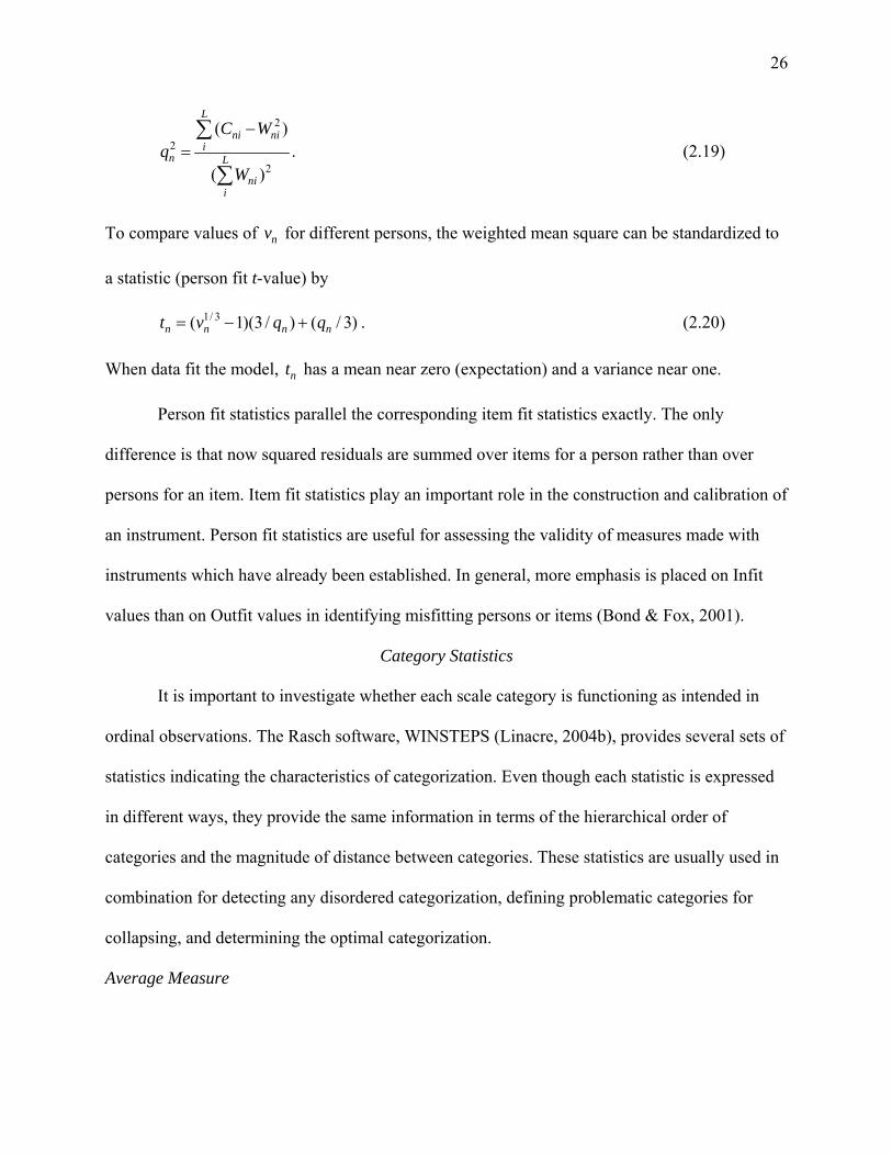
∑. (2.19)

To compare values of for different persons, the weighted mean square can be standardized to

a statistic (person fit t-value) by

nv

1/ 3( 1)(3 / ) ( /n n n nt v q q= − + 3) . (2.20)

When data fit the model, has a mean near zero (expectation) and a variance near one. nt

Person fit statistics parallel the corresponding item fit statistics exactly. The only

difference is that now squared residuals are summed over items for a person rather than over

persons for an item. Item fit statistics play an important role in the construction and calibration of

an instrument. Person fit statistics are useful for assessing the validity of measures made with

instruments which have already been established. In general, more emphasis is placed on Infit

values than on Outfit values in identifying misfitting persons or items (Bond & Fox, 2001).

Category Statistics

It is important to investigate whether each scale category is functioning as intended in

ordinal observations. The Rasch software, WINSTEPS (Linacre, 2004b), provides several sets of

statistics indicating the characteristics of categorization. Even though each statistic is expressed

in different ways, they provide the same information in terms of the hierarchical order of

categories and the magnitude of distance between categories. These statistics are usually used in

combination for detecting any disordered categorization, defining problematic categories for

collapsing, and determining the optimal categorization.

Average Measure

27

Average measure is the empirical average of the measures (i.e., ability of the participants)

observed in a particular category across all items. The average measure is expected to increase

with category value because more of the rating scale is modeled to reflect more of the variable

being measured (Linacre & Wright, 1999). If average measures are not ordered, the specification

that better performers should produce higher ratings is violated.

Step calibration

The Rasch model detects the threshold structure of the Likert-type scale in the data set

rather than presuming the size of the step necessary to move across each threshold. Then the

model estimates a single set of threshold values that apply identically to all of the items in the

scale. In addition to the monotonicity of average measures, step calibration provides useful

information concerning rating scale characteristics. Step calibration is the difficulty estimated for

choosing one response category over the prior response. When the characteristics of

categorization are investigated based on step calibrations, two aspects should be considered. First,

like the average measures, step calibrations are expected to increase monotonically. Second, the

magnitudes of the distances between the threshold estimates in logits should be greater than 1.4

(1.0 for a five response categorization) and smaller than 5.0 because the respective distances

between step calibrations indicate each step’s distinct position on the variable (Linacre, 2002;

Linacre & Wright, 1999).

Category fit statistic

The categories of a scale can be used arbitrarily even with ordered average measures.

Category fit statistic is another criterion for assessing the quality of rating scales. Category fit

provides Infit which is the average of the Infit mean squares associated with the responses in

each category and Outfit which is the average of the Outfit mean squares associated with the

28

responses in each category. For both Infit and Outfit, expected values for all categories are 1.0

and range from 0 to infinity. High Infit indicates that a certain category is chosen when adjacent

categories are expected to be chosen whereas high Outfit mean square indicates that a certain

category is chosen when distant categories are expected to be chosen (Linacre & Wright, 1999).

Values less than 1.0 indicate overly predictable category use for both fit statistics.

In general, Outfit mean squares which are sensitive to outliers are mainly used to

investigate category fit. Outfit mean squares values greater than 2.0 indicate more

misinformation than information (e.g., the value 2.0 indicates half information and half

misinformation). If a category has an Outfit value over 2.0, under the assumption of plausible

linguistic aspects of category definitions, further empirical investigation is required so collapsing

with adjacent categories is recommended.

Reliability Statistics

Items must be well separated and defined to identify the direction and magnitude of a

variable because the variable is measured with test or questionnaire items and expressed in terms

of the scores from the scale (Wright & Masters, 1982). In addition, it is also important to define

how well individual differences are identified with a test or questionnaire. In this regard, the

Rasch model provides two useful indices describing the separation of items on a variable and the

separation of persons on a scale, respectively.

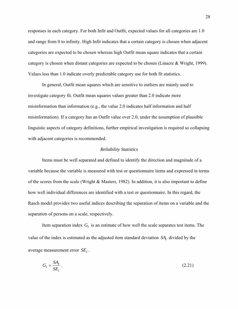
Item separation index IG is an estimate of how well the scale separates test items. The

value of the index is estimated as the adjusted item standard deviation ISA divided by the

average measurement error ISE .

II

I

SAGSE

= . (2.21)

29

The adjusted item standard deviation is simply the root of the adjusted item variance 2ISA

calculated by subtracting the mean square item calibration error IMSE from the observed item

variance 2ISD .

2 2I ISA SD MSE= − I . (2.22)

The observed item variance 2ISD is the variance among calibrations of item difficulty . The

mean square item calibration error

id

IMSE can be obtained by dividing the total error variance of

the items by the total number of items.

2

1

L

ii

I

sMSE

L==∑

. (2.23)

Then the mean square item calibration error is used to obtain an average calibration error.

( )I ISE MSE= . (2.24)

The adjusted item variance 2ISA can be used to estimate the item separation reliability IR which

indicates the replicability of item difficulty across persons.

2 2

2 21(1 )

I II 2

I

I I I

SA MSE GRSD SD G

= = − =+

. (2.25)

The differences between the item separation index and the item separation reliability are that the

latter does not include the measurement error which is not accounted for by the Rasch model,

and that the latter ranges from ranges from 0 to 1.

Person separation index is an estimate of how well the scale identifies individual

differences. The value of the index is estimated as the adjusted person standard deviation

divided by the average measurement error .

PG

PSA

PSE

30

PP

P

SAGSE

= . (2.26)

The adjusted person standard deviation is simply the root of the adjusted person variance 2PSA

calculated by subtracting the mean square person calibration error PMSE from the observed

person variance 2PSD .

2 2P PSA SD MSE= − P (2.27)

The observed person variance 2PSD is the variance among calibrations of person ability . The

mean square person calibration error

nb

PMSE can be obtained by dividing total error variance of

persons by the sample size.

2

1

N

nn

P

sMSE

N==∑

(2.28)

Then the mean square person calibration error is used to obtain an average calibration error.

(PSE MSE= )P (2.29)

The adjusted person variance 2PSA can be used to estimate the person separation reliability PR

which indicates the replicability of person placement across other items measuring the same

construct (Bond & Fox, 2001).

2 2

2 21(1 )

P PP

P P

SA MSE GRSD SD G

= = − =+ 2

P

P. (2.30)

As in the item separation reliability, the measurement error is not included in the equation and

the value of the reliability ranges from 0 to 1.

For item and person separation indices, the greater the value, the better the separation.

For item and person reliabilities, a value close to 1 is considered good reliability because the

31

value indicates the percentage of observed response variance that is reproducible. When both

item and person separation indices are used to determine the optimal categorization, the greater

the separation, the better the categorization because the item will be better separated and the

participants’ differences will be better distinguished.

The Rasch Calibration

In general, the term calibration is defined as the process of defining a measurement

system for an instrument, which provides a frame of reference for interpreting test results. In the

Rasch analysis, the term calibration has been used in various ways. According to Chang’s (1985)

definition, it can be categorized in two ways. In its narrow sense, calibration refers to the part of

or whole processes of estimation of item difficulty parameter values and their standard errors,

placement of items according to their difficulty estimates on a common scale, and estimation of

values for both difficulty and ability parameters. In its broad sense, evaluation of fit to the model

is added to the estimation of difficulty and ability parameters. In current studies of the Rasch

models, the term calibration is commonly used in its broad sense that refers to the process of

converting raw scores to logits to determine the values of item difficulty and person ability in a

metric for the underlying latent trait in addition to the evaluation of models based on various fit

statistics (e.g., Hand & Larkin, 2001; Kulinna & Zhu, 2001; Looney & Rimmer, 2003; Ludlow

& Haley, 1995; Smith, Jr., & Dupeyrat, 2001; Zhu et al., 2001).

The Rasch calibration, which is categorized as a response-centered approach, is known to

provide several advantages over traditional calibration techniques. First, estimations of difficulty

parameter and ability parameter are statistically independent from testing items and samples of

participants employed in the Rasch calibration. This invariance feature is very important in

interpreting testing results because participants’ abilities should remain the same regardless of

32

which testing items are used, and estimates of the difficulty of items are independent of the

particular persons and other items included in the calibration. Second, items and persons are

located respectively along a common scale based on their estimated values. The common scale,

logit, is a ratio scale expressed in probability. Therefore, any difference between examinees and

items on a scale will always have the same stochastic consequence. Subsequently, both

parameters can be interpreted simultaneously within a single framework. Third, after the Rasch

calibration, total scores or subscale scores from ordinal data can be used for additional analyses

because measures provided by the calibration are additive.

The characteristics of the Rasch calibration described in this section provide a solution to

the practical measurement problems in analyzing ordinal data using classical test techniques or

subject-centered approaches. Therefore, applying the Rasch calibration is beneficial and essential

to interpreting rating scales.

Optimal Categorization

It is known that categorization must be ordered according to the magnitude of the trait

and have well-defined boundaries because these features affect the measurement qualities

(Andrich, 1997; Guilford, 1954). These features of categorization are influenced by the amount

of misinformation in a rating scale. Misinformation or noise in rating scales usually results from

the disagreement between participants’ perception and the scale developers’ intention for the

rating scale, or from the absence of generalized and standardized perception of a rating scale

among participants. That is, although scale developers increase the number of response

alternatives to provide participants with more possible responses to choose, participants may fail

to react to a rating scale as the scale developers intended due to the divergent frames of reference

(Roberts, 1994). However, such information, empirically and mathematically, had not been

33

provided with conventional statistics until the Rasch analysis was introduced. Although the

Rasch model was developed for the purpose of objective measurement, the Rasch analysis can

also be used as a post-hoc approach that provides helpful information for testing categorization

function.

The Rating Scale Diagnostics

According to Bond and Fox (2001), several important aspects of categorization function

can be investigated through the Rasch analysis. They suggested that a well-functioning category

rating scale should have enough data (i.e., observed frequencies) in each category to provide

stable estimates for threshold values, hierarchically ordered thresholds, and sufficient category fit

to the model. Even though category function may not be observed in the raw data, these aspects

can be diagnosed through investigating category frequencies, average measures in logits,

threshold estimates, probability curves, and category fit after the initial calibration with the

original categorization.

Inspecting category frequencies for each response option is the first thing done when

examining category function (Andrich, 1996; Linacre, 1995, 2002). Category frequencies

indicate the total number of participants who chose a response category across all items of a

questionnaire. These category frequencies provide information related to observation distribution.

Irregularity such as highly skewed distributions indicates aberrant category usage whereas a

uniform distribution of observations across categories is optimal for step calibration (Linacre,

2002). In addition, frequency of each category is used for detecting low observations affecting

stable estimation of thresholds. Because each threshold is estimated from the log-ratio of the

frequency of its adjacent categories, the estimated scale structure can be highly affected by even

one observation change when category frequency is less than 10 observations (Linacre, 2002).

34

Second, the monotonic increments of average measures can be examined for category function.

Average measures indicate the average of the ability estimates for all participants in a particular

category. Because only one set of threshold estimates are estimated for all items in a

questionnaire, the average measure of a certain category can be interpreted as the average ability

estimate in logits for participants who chose the category on any item in the questionnaire.

Therefore, observations in higher categories must be produced by higher measures. In other

words, average measures reflect the pattern of monotonic increment when participants with

lower ability or attitude choose the lower categories and participants with higher ability or

attitude choose the higher categories. Third, thresholds are the difficulties estimated for choosing

one response category over another. Like the average measures, thresholds should increase

monotonically. If thresholds do not increase monotonically across the rating scale, categories are

considered disordered which reflects the low probability of observing certain categories and

which decreases the interpretability of the resulting measures. Thresholds can be inspected based

on either the threshold estimates or the probability curves. Linacre (2002) suggested that

thresholds for a rating scale with five response options should advance by at least 1.0 logits to

show distinction between categories, but not more than 5.0 logits to avoid large gaps, called

‘dead zone’, in the middle of the category in which a measurement loses its precision. When

inspecting category curves, each category should have a distinct peak in the probability curve

graph. Because threshold estimates correspond to the intersection of adjacent category curves, a

category without a distinct peak cannot be the most probable response category for some portion

of the measured variable which results in disordered thresholds. Finally, investigating category

fit expressed in terms of Outfit mean square is useful for assessing the quality of category

35

function. An Outfit mean square value greater than 2.0 indicate that there is more unexplained

information than explained information in the observation of the category.

Even though these diagnostics provide the same information in different ways, it is

recommended to use the diagnostics in combination to detect problems in category function.

When any violation is found, collapsing adjacent categories is recommended to increase the

reliability and validity of the measure.

Collapsing Categories

The purposes of collapsing categories are to minimize misinformation across categories,

to improve variable clarity, and to derive the optimal categorization. If problems such as

infrequently used categories, category disorder, and poorly defined boundaries are found in

categorization, it is recommended to combine the problematic response category with adjacent

category (Bond & Fox, 2001; Linacre, 2002). Therefore, revising the rating scale starts from

deriving new combinations from the original categorization.

There are two ways to collapse categories although both methods employ the identical

Rasch diagnostic procedures. The first method is to collapse only categories having category

function problems up or down with adjacent category. This method is recommended when it is

obvious that deriving only a limited number of combinations leads to an optimal categorization.

Another method, called mechanical way in Zhu and Kang’s (1998) study, is that all possible

combinations are derived from the original categorization. For example, Zhu and Kang (1998)

recombined the original five adjacent categories into two, three, and four categories in their

Rasch analysis using a self-efficacy scale. All 15 categorizations including fourteen sets of

derived categorizations and the original categorization were analyzed individually. Even though

this mechanical way requires repeating the same protocol until all derived data sets are analyzed,

36

all possible combinations can be compared. The mechanical way is preferred when researchers

are uncertain of the exact number of response categories to be collapsed into because any

features or characteristics of the optimal categorization cannot be observed from the raw data.

Once the collapsing formats are determined, the Rasch analysis is applied to all the data

sets recombined. Each categorization is examined and compared based on category information

and statistics provided by the Rasch analysis. First, model-data fit statistics are examined to

investigate how many items and persons are misfit in terms of Infit and Outfit, and to determine

whether a categorization is acceptable for further comparison and investigation. Second,

category average measures and threshold estimates are examined to inspect the order of each

categorization. Finally, the categorizations with hierarchical order are compared based on item

and person separation indices. From the final comparisons, the categorization with the greatest

separation values is chosen for the optimal categorization.

Measurement of Body Image

The importance of understanding body image has increased because it is known that

dissatisfaction with body image is significantly related to the development of eating disorders

such as anorexia nervosa and bulimia nervosa (Brown, Cash, & Lewis, 1989; Thompson, 1996;

Williamson, Cubic, & Gleaves, 1993) and perceived body image influences exercise motives and

adherence (Ingledew & Sullivan, 2002). In this regard, body image has been studied in terms of

body size and appearance, dissatisfaction, physique anxiety, and social pressure. Instruments and

techniques have been recently developed or revised to measure body image constructs.

Due to the implicit nature of body image, the term body image has been used to describe

a wide range of body-related constructs but some researchers have used the term to indicate a

very specific concept of body. Even though there is still disagreement in defining body image,

37

Rowe (1996) categorized instruments measuring body image into two types. Instruments in the

first category have been devised for measuring size-perception accuracy which is related to the

ability to estimate the size of one’s own body in a whole or part (e.g., Askevold, 1975; Freeman,

Thomas, Solyom, & Hunter, 1984; Ruff & Barrios, 1986; Slade & Russell, 1973). On the other

hand, instruments in the second category have been developed for measuring cognitive-affective

aspect of body image. Different from size-perception accuracy measurement, participants’

attitudes toward the body and physical appearance are of interest in measurement of cognitive-

affective aspect (e.g., Cash, Winstead, & Janda, 1986; Garner, Olmstead, & Polivy, 1983; Kurtz,

1969). In measuring participants’ attitudes toward body image, which is the assessment of the

cognitive-affective dimensions of body image, the most common type of instruments has been

questionnaires (Baumgartner et al., 2003; Rowe, 1996).

Currently, it is common for researchers to use a part of a previous instrument or several

different instruments in combination to measure an expected trait such as eating disorders, social

pressure, and exercise adherence (e.g., Hausenblas & Fallon, 2002; Ingledew & Sullivan, 2002;

Stice, Maxfield, & Wells, 2003). For example, Hausenblas and Fallon (2002) used a multitude of

instruments in the investigation of the relationship among body image, exercise behavior, and

exercise dependence symptoms in physically active individuals. In their study, a subscale (i.e.,

Drive for Thinness) of the Eating Disorder Inventory-2 (Garner, 1991), the Leisure-Time

Exercise Questionnaire (Godin, Jobin, & Bouillon, 1986), selected items from the

Multidimensional Body-Self Relations Questionnaire (Cash, 1990), the Social Physique Anxiety

Scale (Martin, Rejeski, Leary, McAuley, & Bain, 1997), and 21 revised items from the DSM-IV

(Hausenblas & Symons Downs, 2001) were employed to measure weight preoccupation, the

38

frequency of exercise, the subjective component of body image, physique anxiety, and exercise

dependency, respectively.

Characteristics of Body Self-Image Questionnaire

Several issues concerning instruments measuring body image have been identified such

as a theoretical foundation is insufficient to develop body image measurement instruments, the

concept of body image being measured is not declared explicitly, and existing instruments lack

of psychometrically sound methods and construct validity evidence (Baumgartner et al., 2003;

Rowe, 1996; Thompson, 1996). For example, no conceptual explanation or any empirical

evidence is provided either for the original version or the revised formats of the Body Self-

Relations Questionnaire (Cash, 1990) although the original and revised instruments have been

widely used. Consequently, the instruments produce ambiguity and doubt in the interpretation of

research results.

Rowe (1996) developed a questionnaire because of the need for an explicit foundation of

body image and empirical evidence of construct validity. In his study, the nature of the body

image construct was investigated and the BSIQ was developed and validated to measure body

image in college students. Data were collected through four stages. Responses to open-ended

questions administered in the first pilot stage were used to develop statements for the

questionnaire. In the second and third pilot stages, exploratory factor analyses and item-subscale

correlations were used to guide revisions to the questionnaire. The final stage involved the

collection of evidence to support the construct validity of the questionnaire. In the final stage,

observations from 1024 undergraduate students were randomly divided into two subsamples.

Confirmatory factor analysis (CFA) was applied to a subsample (i.e., calibration sample) for

calibration in which the measurement model underlying the questionnaire was modified. The

39

result of the CFA supported acceptable fit for a nine-factor model with 39 items. The model was

also cross-validated with the other subsample (i.e., validation sample) by imposing the parameter

values from the calibration sample on the validation sample data. After the model was generated,

t-tests were conducted to provide discriminant evidence of construct validity. Discriminant

evidence of construct validity was obtained by comparing the females in the final sample to

additionally collected samples; female students with eating disorders and female students who

were dancers. Mean scores of the students with eating disorders indicated that they evaluated

their overall appearance, health/fitness level, and fatness more negatively, and expressed more

negative feelings about their bodies than the students in the final sample. On the other hand, the

student dancers’ mean scores indicated that they evaluated their overall appearance, fatness level,

and health/fitness level more positively, and expressed less negative feelings about their bodies

than the students in the final sample.

The Rasch Analysis for Measurement Problems of Body Image Instruments

Most instruments for the cognitive-affective domain of body image have been

questionnaires and Likert-type response options have been employed for those instruments. As

pointed out by Rowe (1996), many instruments have failed to provide psychometric evidence

despite the instruments are commonly used in practice. The BSIQ was developed with the

researcher making an effort to eliminate the shortcomings of previous body image questionnaires

such as insufficient understanding of body image constructs and the lack of reliability and

validity evidence. Although providing the psychometric evidence may seem to reduce or

eliminate the shortcomings and to improve the quality of the instrument, some fundamental

measurement issues arise because ordinal data from the Likert-type scale were directly used for

analyses. Ordinal data are not sufficiently interval to justify the arithmetical calculations

40

employed by t-tests and factor analysis (Wright, 1996). Additionally, categorization affects the

quality of an instrument that is directly related to the distribution of the data. However, it is not

known whether the five-point category options functioned as intended because no statistical or

empirical evidence is provided from the conventional procedures used in the study.

Applying the Rasch model to the analysis of rating scales have several advantages in

solving those measurement problems. The Rasch calibration transforms the ordinal data, more

specifically both item difficulty and person ability (i.e., body image satisfaction) into logits

which have the same characteristics of interval data. Therefore, not only calculating total scores

but also comparing both facets simultaneously on the same metric is possible, which were not

possible with the conventional statistics in Rowe’s (1996) study. This transformation also

enables researchers to do further statistical analysis such as comparison of two diverse groups for

construct validity without linearity concerns. Another advantage of the Rasch analysis is that

optimal categorization can be determined for the BSIQ in an empirical way because it provides

information for testing categorization function. Because the Rasch analysis is used for detecting

optimal categorization as a data-based and post-hoc approach, it generates all possible

combinations of categorization from the original data instead of requiring that additional data

with several sets of predetermined categorization be collected.

41

CHAPTER 3

PROCEDURES

The primary purpose of this study was to calibrate the BSIQ (Rowe, 1996) to construct an

objective and additive scale by transforming the raw data from an ordinal scale into logits using

the Rasch analysis. The secondary purpose was to determine the optimal categorization for each

subscale of the BSIQ. Procedures included (a) calibrating the BSIQ initially to determine the

optimal categorization, (b) constructing items with acceptable fit statistics in each subscale (i.e.,

factor), (c) validating the model using a smaller sample, and (e) describing item difficulty and

person ability (i.e., body image satisfaction) on the same continuum. In addition, groups formed

based on body mass index (BMI) were examined for differences in logits as evidence of

construct validity of the questionnaire. Procedures and descriptions of the data analysis are

provided in Table 1.

Data and Instrument

Data

In this study, data from a previous body image study were used with permission from the

researcher (Rowe, 1996). Data were collected from male and female undergraduate students who

were participating in physical education activity classes at the University of Georgia. Rowe

(1996) intended to sample from various types of classes because personal status such as previous

fitness experience and attitude might be related to the choice of class.

42

In the present study, the total sample, which included 1021 participants, was used for the

Rasch calibration. Additionally, a smaller sample, the validation sample, was generated

randomly from the total sample for confirming the revised categorization and the retained items

and for providing evidence of construct validity. Demographic information for the total sample

and the validation sample are presented in Table 2.

The Body Self-Image Questionnaire

The questionnaire used in the present study was originally developed for measuring body

self-image in undergraduate students (Rowe, 1996). In Rowe’s study, a total of 56 items were

initially administered to the participants and 39 items under nine factors were retained with

acceptable fit based on factor analyses. A Likert-type five-point scale (Not at all true of myself =

1, Slightly true of myself = 2, About halfway true of myself = 3, Mostly true of myself = 4, and

Completely true of myself = 5) was used for all items. Therefore, the BSIQ consists of 39 items

with a Likert-type five-point scale under nine factors including overall appearance evaluation,

fatness evaluation, health/fitness evaluation, negative affect, health/fitness influence, social

dependence, investment in ideals, attention to grooming, and height dissatisfaction. Because the

BSIQ was developed to measure the multidimensional constructs of body image, it was not

intended by Rowe to obtain a total score from the questionnaire, rather the subscale scores from

each factor were of interest in investigating university students’ body self-image related

constructs. Therefore, the nine subscales using the factors of the BSIQ were calibrated separately

for the Rasch analysis.

The procedures in detail for developing the BSIQ are described in the related research.

The thirty-nine items and the response format for the BSIQ are presented in Appendix A and the

nine factors with related items are provided in Appendix B.

43

Data Analyses

The RSM was employed in the present study and the model was applied to the BSIQ data

for calibrating ordinal data, investigating category function, determining optimal categorization,

and constructing items for each subscale. The validation sample was analyzed to conduct cross-

validation and construct validity studies.

Calibration

Nine subscales of the BSIQ, overall appearance evaluation (OAE), fatness evaluation

(FE), attention to grooming (AG), health/ fitness evaluation (HFE), health/ fitness influence

(HFI), social dependence (SD), height dissatisfaction (HD), negative affect (NA), and investment

in ideal (II), were separately calibrated using the RSM. For the initial calibration, no

modification was made in the categorization and the number of items for each subscale.

Category Function

The Rasch analysis was applied to the BSIQ to determine whether the Likert-type five-

point scale was optimal or some other response format was more appropriate for the data. Since

the best categorization would not be observed in the raw data, category function from the initial

calibration was examined to determine whether the Likert-type five-point scale was ordered with

increasing or decreasing numerical trait.

Linacre (2002) introduced useful guidelines for optimizing rating scale category

effectiveness. The guidelines were used in the present study for investigating category function.

The description of the guidelines used in the present study is summarized in Table 3.

For a categorization with any violation according to the guidelines, a collapsing process

was applied to combine the original five categories into three or four categories in order to

improve the overall measurement quality. For example, Zhu, Timm, and Ainsworth (2001)

44

calibrated a 23-item exercise barrier instrument with the Rasch analysis and they collapsed the

original five categories (i.e., Very Often, Often, Sometimes, Rarely, and Never) into three and

four categories in their study. The collapsing combinations were 11123, 11233, 11223, 12223,

12233, and 12333 for three categories, and 11234, 12234, 12334, and 12344 for four categories.

For example, the collapsing combination 11123 is combining the first three categories to become

a score of 1, the fourth category becomes a score of 2, and the fifth category becomes a score of

3. However, it should be cautioned that information may be lost if a positive response category

and a negative response category are combined into a category. For example, Zhu and colleagues

combined the Often, Sometimes, and Rarely categories into a new category in a combination

12223. While this combining may increase fit statistics, it may be meaningless in terms of

interpreting the respondents’ perceived construct on the categorization.

Therefore, in the present study, only the categories that violated category count,

hierarchal order, and the step calibration advance were combined with adjacent categories as

suggested by Linacre (2002) instead of trying to combine based on all possible combinations.

First, in each subscales, categorization with acceptable Outfit mean squares (< 2.0), category

counts more than 10 responses in each category, hierarchically ordered average measures and

step calibrations, and step calibration advances equal or larger than 1.0 logit and smaller than 5.0

logits were retained as appropriate for corresponding subscales.

Second, categories with any violation of the criteria described in Table 3 were combined

with adjacent categories (i.e., k-1 category) then the data with the collapsed categorization were

recalibrated. When two or more collapsing combinations existed in a subscale, the combination

with the category fit statistics closer to 1.0 mean square, and with better item and person

separation statistics was retained as the optimal categorization for the subscale. Item and person

45

separation statistics provide information concerning how well a scale separates testing items and

participants, respectively (Wright & Masters, 1982). For item and person separation statistics, the

larger the value of the indices, the better the separation.

Misfitting Item Deletion

Item fit statistics were investigated to determine which items to delete for each subscale.

Acceptable ranges for both Infit and Outfit mean squares were set at .60 ≤ fit ≤ 1.40 which was

suggested for rating scales with Likert-type responses by Bond and Fox (2001). After the

deletion of misfitting item(s) from a subscale, the data with the retained items were recalibrated

to investigate item fits and to obtain parameter estimates.

Cross-Validation

The modification in the categorization and the structure of a rating scale may be sample

dependent. The RSM was applied to the data of the validation sample for confirming that the

categorization retained or revised for each subscale and the retained items in each subscale were

acceptable. The validation sample was generated from the total sample (N = 1021) by selecting

510 participants randomly using the SPSS program.

First, the category function for each subscale was examined based on category frequency,

average measure, step calibration, and Outfit statistic with the same criteria used in the

collapsing process for the total sample. Then, the pattern of categorization for the validation

sample was compared to the pattern of categorization for the total sample. Second, to investigate

the stability of the Rasch estimation for item difficulty, the hierarchical order of items for the

total and validation samples were compared for each subscale.

46

Construct Validity

Body mass index (BMI) has been widely used to estimate body composition in field

settings (Baumgartner et al., 2003). Based on the research literature, the degrees of body

dissatisfaction and social physique anxiety are influenced by the level of BMI of individuals.

Even though BMI has a high predictive error especially when physically active males with high

lean body mass are measured, many researchers have suggested that BMI is significantly

associated with body dissatisfaction (Ingledew & Sullivan, 2002; Pietrobelli, Faith, Allison,

Gallagher, Chiumello, & Heymsfield, 1998). Hausenblas and Fallon (2002) also reported that

BMI was the positive predictor of body dissatisfaction and social physique anxiety for females.

According to American College of Sports Medicine’s (ACSM) guidelines, obesity-related health

problems increase beyond a BMI of 25 for most people (ACSM, 2000). World Health

Organization defines a BMI between 18.5 and 24.9 as normal, 25 to 29.9 as overweight, and 30

or greater as obesity (Baumgartner et al., 2003).

To test if the BSIQ measures reflect a related abstract trait (i.e., body image satisfaction

or dissatisfaction) which is influenced by BMI after calibration and revision, a construct validity

approach was employed with a statistical test of mean difference among groups. The validation

sample was divided into three groups based on each participant’s BMI; underweight (< 18.5),

normal (18.5~24.9), and overweight (25 or higher). Descriptives for the three groups are

presented in Table 4. The group mean differences of person measures in logits generated from

the Rasch calibration in each subscale were examined. One-way analysis of variance (ANOVA)

with alpha level of .05 was used for investigating group mean difference. Consequently, the

group means were contrasted using the t-test for two independent groups to examine which

groups significantly differenced. To reduce the cumulative type I error, the alpha level of .05 was

47

divided by the number of contrasts for each subscale (Keppel, 1991). The rounded alpha level of

.02 was used for the contrasts.

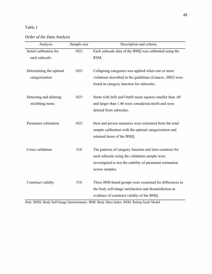
48

Table 1

Order of the Data Analysis

Analysis Sample size Description and criteria

Initial calibration for

each subscale

1021 Each subscale data of the BSIQ was calibrated using the

RSM.

Determining the optimal

categorization

1021 Collapsing categories was applied when one or more

violations described in the guidelines (Linacre, 2002) were

found in category function for subscales.

Detecting and deleting

misfitting items

1021 Items with Infit and Outfit mean squares smaller than .60

and larger than 1.40 were considered misfit and were

deleted from subscales.

Parameter estimation 1021 Item and person measures were estimated from the total

sample calibration with the optimal categorization and

retained items of the BSIQ.

Cross-validation 510 The patterns of category function and item construct for

each subscale using the validation sample were

investigated to test the stability of parameter estimation

across samples.

Construct validity 510 Three BMI-based groups were examined for differences in

the body self-image satisfaction and dissatisfaction as

evidence of construct validity of the BSIQ.

Note. BSIQ: Body Self-Image Questionnaire. BMI: Body Mass Index. RSM: Rating Scale Model

49

Table 2

Characteristics of the Participants

Characteristic Total Sample (N = 1021) Validation Sample (n = 510)

Gender

Male Female

Grade Freshman Sophomore Junior Senior

Ethnic African-American Asia-American Caucasian Other ethnic

Descriptives Mean age (SD) Mean height (SD) Mean weight (SD) Mean BMI (SD)

431 (42.2%) 590 (57.8%)

209 (20.5%) 473 (46.3%) 237 (23.2%)

101 (9.9%)

71 (7.0%)48 (4.7%)

845 (82.5%) 46 (4.5%)

19.91 (1.42) 67.49 (4.16)

147.74 (32.33)22.69 (3.97)

211 (41.4%) 299 (58.6%)

93 (18.2%)250 (49.0%) 123 (24.1%)

43 (8.4%)

32 (6.3%)22 (4.3%)

427 (83.7%) 21 (4.1%)

19.88 (1.37) 67.47 (4.05)

147.88 (31.98)22.74 (3.99)

Note. BMI: Body Mass Index. Validation sample was randomly extracted from the total sample. Height was in

inches. Weight was in pounds.

50

Table 3

Guidelines for Optimizing Category Effectiveness

Guideline Description

At least 10 observations in each

category

Lower observation may result in imprecise estimate of step

calibration because it is estimated from the log-ratio of the

frequency of its adjacent categories.

Hierarchically ordered average

measure

Disorder in average measure may result when a lower category is

dominantly chosen by participants with higher measures or a

higher category is chosen by participants with lower measures.

Outfit mean square less than 2.0 If Outfit mean square for a category is larger than 2.0, the

categorization is unproductive for construction of measurement

and distorts and degrades the measurement system.

Hierarchically ordered step

calibration

Disorder in step calibration may result if a lower category is

chosen by participants with higher measures and vice versa.

The advance between step

calibrations ≥ 1.0 logit

For a five category rating scale, advances of at least 1.0 logits

between step calibrations are needed in order for that scale to be

equivalent to four separate dichotomies, and to have wider

substantive meaning.

The advance between step

calibrations ≤ 5.0 logits

If the step calibrations are more than 5 logits apart, the scale

provides less information about the participants.

51

Table 4

Characteristics of the Three Groups Based on Body Mass Index (BMI) in the Validation Sample

Underweight (n = 36) Normal (n = 365) Overweight (n = 102)

Male 3 143 60

Female 33 222 42

Age 19.62 ( .74) 19.86 ( 1.36) 20.07 ( 1.56)

Height 65.92 ( 2.87) 67.53 ( 3.92) 67.79 ( 4.75)

Weight 107.25 (13.65) 141.10 (21.66) 186.68 (32.57)

BMI 17.30 ( 1.37) 21.65 ( 1.75) 28.55 ( 4.32)

Note. BMI: body mass index. Missing cases = 7. Values in parentheses are standard deviation. Height was in inches.

Weight was in pounds.

52

CHAPTER 4

RESULTS AND DISCUSSION

The BSIQ data were analyzed with the RSM. The category function and item structure

for each subscale were investigated. Subsequently, the RSM was applied to the validation sample

to investigate the model sensitivity to sample size change and to confirm the revised

categorization and item structure. Finally, three BMI-groups were compared using the person

parameter estimates from the RSM for evidence of construct validity.

Rating Scale Model Calibration

The first assumption for Rasch analysis is that a scale is unidimensional. Even though the

BSIQ was divided into nine subscales based on factor analysis in which each subscale

represented one independent unidimensional scale, the data were analyzed to confirm the

unidimensionality of each subscale using principal component analysis in the SPSS program.

From principal component analysis, only one component (i.e., factor) was extracted in each

subscale. The percents of variance explained by the extracted component were from 58.07 to

82.47 for the nine subscales.

Each subscale with the original categorization and items was calibrated using the RSM.

The results from the initial calibration were examined to determine the optimal categorization

and to detect misfitting items.

53

Categorization

The RSM was found to be a good fit in the initial calibration for the categorizations of all

subscales in regard to frequencies, hierarchical order in average measures and step calibrations,

and Outfit mean squares. No disordered categories were found in terms of average measures and

step calibrations in the initial calibration. However, step calibrations for the FE, SD, HD, and II

subscales didn’t advance enough as suggested in the guidelines (Linacre, 2002). In Table 5, the

distance between the categories 3 and 4 was narrower than 1.0 logit for the SD, HD, and II

subscales (see step advance values). For the FE subscale, the advances between the categories 3

and 4 and between the categories 4 and 5 were less than 1.0 logit. Therefore, collapsing process

was applied to the categorization of these four subscales.

Combining the categories 3 and 4 into one category (recoded as 12334) was applied to

the SD, HD, and II subscales because only one violation of step calibration advance was found

on the third step calibration for each subscale. For the FE subscale, three collapsing

combinations combining the (a) categories 3 and 4 (recoded as 12334), (b) categories 4 and 5

(recoded as 12344), and (c) categories 3, 4, and 5 (recoded as 12333) were applied.

Information about corresponding average measures, Outfit mean squares, and step

calibrations for the collapsed four-point categorization are presented in Table 6. For the SD, HD,

and II subscales, combining the categories 3 and 4 was acceptable based on the guidelines and

improved category function. After the collapsing, average measures and step calibrations were

ordered in respective subscales as observed in the initial calibration. For the SD subscale, step

calibrations were -2.35, -.74, and 3.09 for thresholds between the first and second, second and

third, third and fourth categories, respectively. All advances between step calibrations were

54

larger than 1.0 logit. For the HD subscale, step calibrations were -2.77, -.67, and 3.45. For the II

subscale, step calibrations were -2.29, -.87, and 3.16.

For the FE subscale, combining the categories 3 and 4 (i.e., 12334) was better than other

collapsing combinations because all measures were ordered and step calibrations (-1.61, -.48,

and 2.10) advanced enough (1.13 and 2.58). In addition, the combination 12334 provided better

statistics such as person separation (2.34), person reliability (.85), item separation (18.81), and

item reliability (1.00). In contrast, the combination 12344 still resulted in a small advance

between the second (.43) and third (.56) step calibrations. Even though no violation of category

function was found in the combination 12333, collapsing five categories into three resulted in the

loss of information about respondents (person separation = 1.85; person reliability = .77) and

slightly deteriorated the quality of the subscale (item separation = 17.47) compared to

combination 12334. Therefore, a collapsed categorization combining the categories 3 and 4 was

chosen for the FE, SD, HD, and II subscales while the original five-point categorization was

retained for the OAE, AG, HFE, HFI, and NA subscales. The graphs representing the changes

after the collapsing categories for the SD, HD, and II subscales are presented in Figures 1, 2, and

3, respectively. Because the misfitting item treatment was required for the FE subscale, the

category probability curves for the subscale are presented in the next section.

Misfitting Item Deletion

Item fit statistics were examined to detect misfitting items after investigating the category

function of each subscale and determining the optimal categorization for the subscales with

problematic categorization. Any items which had Infit and Outfit statistics smaller than .6 or

larger than 1.4 were considered misfit.

55

In the FE subscale, two misfitting items were found. Fit statistics for item 22 (I have large

buttocks) were 1.62 for Infit mean square and 1.66 for Outfit mean square. Item 35 (My stomach

is flabby) was also misfitting and fit statistics for this item were 1.44 and 1.51 for Infit and Outfit

mean squares, respectively. Because these fit statistics for item 22 and 35 were obtained after

categories 3 and 4 were combined and these two items were also misfitting with the original five-

point categorization (Infit = 1.72 and Outfit = 1.80 for item 22; Infit = 1.42 and Outfit = 1.55 for

item 35), an investigation as to what caused this was conducted. It might be that the pattern of

category function of misfitting items, which worked differently from the categorization of the

other fitting items, affected the category function of the FE subscale. If this is true, it might not

be necessary to collapse the original five-point categorization into four when the two misfitting

items were deleted from the FE subscale. To investigate this concern, the function of the original

five-point categorization for the FE subscale was again checked after items 22 and 35 were

deleted without collapsing any categories. As a result, no disordered measures were found but

the step calibrations for the original categorization were -2.18, -.26, .57, and 1.88 indicating that

the advance between the second and third step calibration was smaller than 1.0 logit. This result

supported collapsing the third and fourth categories for the FE subscale. Therefore, items 22 and

35 were deleted from the FE subscale and the collapsed categorization (12334) was kept without

further concerns. The data were recalibrated for the FE subscale with items 22 and 35 deleted

from the subscale and with the collapsed four-point categorization to obtain the category

function statistics. All measures were ordered and each step calibration advanced larger than 1.0

logit. The final category function statistics for the FE subscale are presented in Table 7. The

category probability curves for the FE subscale representing the change of categorization after

collapsing categories and item deletion are presented in Figure 4.

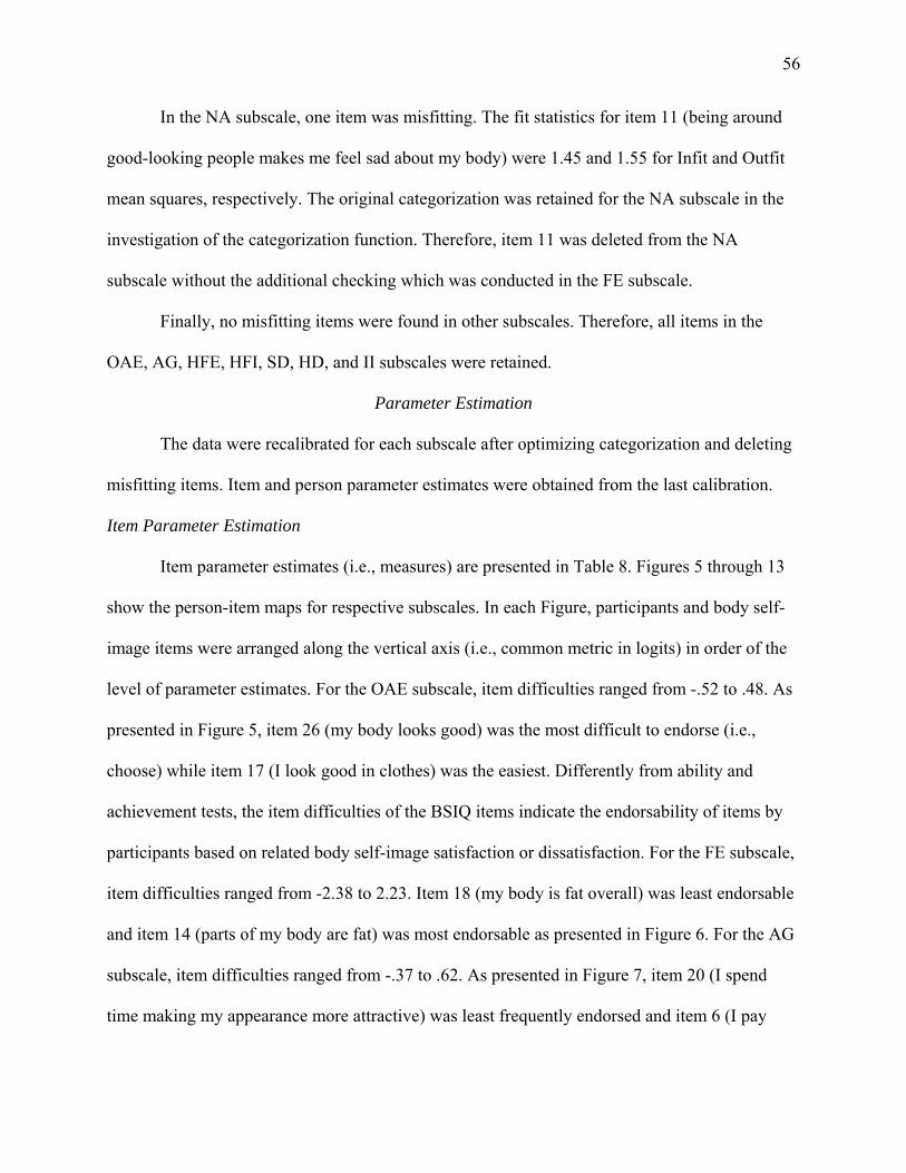
56

In the NA subscale, one item was misfitting. The fit statistics for item 11 (being around

good-looking people makes me feel sad about my body) were 1.45 and 1.55 for Infit and Outfit

mean squares, respectively. The original categorization was retained for the NA subscale in the

investigation of the categorization function. Therefore, item 11 was deleted from the NA

subscale without the additional checking which was conducted in the FE subscale.

Finally, no misfitting items were found in other subscales. Therefore, all items in the

OAE, AG, HFE, HFI, SD, HD, and II subscales were retained.

Parameter Estimation

The data were recalibrated for each subscale after optimizing categorization and deleting

misfitting items. Item and person parameter estimates were obtained from the last calibration.

Item Parameter Estimation

Item parameter estimates (i.e., measures) are presented in Table 8. Figures 5 through 13

show the person-item maps for respective subscales. In each Figure, participants and body self-

image items were arranged along the vertical axis (i.e., common metric in logits) in order of the

level of parameter estimates. For the OAE subscale, item difficulties ranged from -.52 to .48. As

presented in Figure 5, item 26 (my body looks good) was the most difficult to endorse (i.e.,

choose) while item 17 (I look good in clothes) was the easiest. Differently from ability and

achievement tests, the item difficulties of the BSIQ items indicate the endorsability of items by

participants based on related body self-image satisfaction or dissatisfaction. For the FE subscale,

item difficulties ranged from -2.38 to 2.23. Item 18 (my body is fat overall) was least endorsable

and item 14 (parts of my body are fat) was most endorsable as presented in Figure 6. For the AG

subscale, item difficulties ranged from -.37 to .62. As presented in Figure 7, item 20 (I spend

time making my appearance more attractive) was least frequently endorsed and item 6 (I pay

57

careful attention to my face and hair, so that I will look good) was most frequently endorsed. For

the HFE subscale, item difficulties ranged from -1.13 to .58. As presented in Figure 8, item 34 (I

have an athletic build) was least endorsable while item 13 (my body is healthy) was most

endorsable. For the HFI subscale, item difficulties ranged from -1.42 to .91. Item 36 (my body

image is influenced by the state of my health) was least frequently endorsed while item 30 (the

way I feel about my body improves when I exercise regularly) was most frequently endorsed as

presented in Figure 9. For the SD subscale, item difficulties ranged from -.18 to .25. As

presented in Figure 10, item 4 (my thoughts about my body depend on the clothes I’m wearing)

was least frequently endorsed and item 8 (I compare my body to people I’m close to) was most

frequently endorsed. For the HD subscale, item difficulties ranged from -.64 to .72. As presented

in Figure 11, item 38 (if I were a different height, I’d like my body better) was least endorsable

and item 2 (I’ve often wanted to be taller) was most endorsable. For the NA subscale, item

difficulties ranged from -.52 to .69. Item 19 (my naked body makes me angry) was least

endorsable and item 5 (my naked body makes me feel sad) was most endorsable (Figure 12). For

the II subscale, item difficulties ranged from -.58 to .59. As presented in Figure 13, item 16

(muscle definition is important to me) was least endorsable while item 9 (having a well-

proportioned body is important to me) was most endorsable among the II items.

Person Parameter Estimation

Person parameter estimates, also called person abilities, were obtained from the final

calibration for each subscale. In this study, person abilities indicate the perceived level of body

self-image satisfaction or dissatisfaction. For subscales inquiring body self-image satisfaction

(e.g., OAE, HFE, and HFI), higher measures imply higher satisfaction and vice versa. As

mentioned in earlier section, person parameter estimates were calibrated on the metric where

58

item parameter estimates were located. Therefore, it was possible to compare person and item

measures on the same yardstick. In addition, the parameter estimates, person and item measures,

were interval-level data transformed from ordinal-level data by the Rasch calibration. Therefore,

measures were used for the analysis of group mean difference in which the linearity of data was

assumed.

Validation

From the cross-validation process, the optimal categorization was examined with the

same criteria used in the collapsing process and the stability of item structure of the BSIQ was

cross-validated by investigating the pattern of item difficulties in each subscale.

If the hierarchical item order and item fit statistics differ largely in spite of the invariance

feature of IRT, the items would represent different constructs to each sample of participants and

would limit quantitative comparisons (Andrich, 1988). In addition, consistent categorization

across the samples would confirm the participants’ stable perception of the categorization of the

BSIQ.

Cross-Validation with Reduced Sample Size

Cross-validation was conducted to examine the patterns of categorization and retained

items of the BSIQ using a smaller sample (the validation sample, n = 510) that was randomly

selected from the total sample. The RSM model was applied to the validation sample with the

revised categorization and items. This procedure was done to confirm the optimal categorization

of each subscale, and to investigate the stability of item parameter estimates and the sensitivity of

the model to the smaller sample size.

59

Categorization

The patterns of the categorizations for each subscale in the validation sample were

similar to the categorizations for each subscale in the total sample. For the OAE, AG, HFE, HFI,

and NA subscales, the original five-point categorization was kept for the total sample. The

results from the calibration using the cross-validation sample were also consistent with the

categorizations in the total sample. Average measures and step calibrations were hierarchically

ordered. Outfit mean squares for categories for each subscale were within the criterion of 2.0.

Step calibrations were -4.08, -1.65, 1.15, and 4.58 for the OAE, -3.74, -1.04, .92, and 3.86 for the

AG, -3.12, -1.35, .73, and 3.75 for the HFE, -2.12, -.98, .76, and 2.34 for the HFI, and -3.02, -

.53, .93, and 2.62 for the NA subscale. All steps for each subscale advanced more than 1.0 and

less than 5.0 logits.

For the FE subscale, two items (I22 and I35) were misfitting in the validation sample as

in the total sample calibration. Therefore, the two missing items were deleted for the

recalibration. For the FE subscale, the collapsed four-point categorization (i.e., combination

12334) was chosen for the total sample. The collapsed four-point categorization also worked

well for the validation sample. Average measures and step calibrations were hierarchically

ordered and Outfit mean squares for each category (1.02, .83, 1.07, and 1.06) were within the

criteria. The step calibrations were –2.58, -.43, and 3.00 so, each step advance between step

calibrations met the criteria. Because the collapsed categorization drawn from the total sample

was applied to the validation sample for the FE subscale, the category function of the original

five-point categorization was also checked again using the validation sample. The results were

identical with the total sample calibration. Items 22 and 35 were misfitting and step calibrations

were -1.43, -.11, .39, and 1.16 indicating that step advances between the second and third and

60

between the third and fourth step calibrations were smaller than 1.0 logit. Therefore, the

collapsed four-point categorization was confirmed for the FE subscale in the validation sample.

For the SD subscale, the collapsed four-point categorization (combination 12334) worked

well for the validation sample. All average measures and step calibrations were ordered and all

step advances were larger than 1.0 and smaller than 5.0 logits (-2.35, -.78, and 3.13). In

calibration with the original five-point categorization, however, step advance between the second

and third step calibrations was smaller than 1.0 logit. Therefore, the collapsed combination

12334 was confirmed for the SD subscale in the validation sample.

For the HD subscale, the collapsed four-point categorization (combination 12334) was

working well in the validation sample. All average measures and step calibrations were ordered

and all step advances were larger than 1.0 and smaller than 5.0 logits (-2.87, -.77, and 3.64). In

calibration with the original five-point categorization, however, the original five-point

categorization also worked well in terms of hierarchically ordered measures and step calibrations,

Outfit statistic, and step advances. Subsequently, separation statistics for the original and

collapsed categorizations were compared to determine which categorization discriminated items

and persons better for the HD subscale in the validation sample. Person separation statistics were

1.67 for the original categorization and 1.51 for the collapsed. In the comparison of item

separation, the original categorization (5.89) provided a better statistic than the collapsed (5.14).

Therefore, the collapsed four-point categorization chosen from the total sample calibration for

the HD subscale was not confirmed in the validation sample.

For the II subscale, the collapsed four-point categorization (combination 12334) was

chosen in the total sample calibration and the collapsed categorization was confirmed in the

validation calibration. All average measures and step calibrations were ordered and Outfit mean

61

squares for categories were within the criteria. Step advances were -2.48, -.80, and 3.28 so, all

steps advanced more than 1.0 and less than 5.0 logits. In checking again the optimal

categorization for the II subscale, step calibrations for the original categorization were -2.29, -

.26, .37, and 2.18 indicating the narrow distance (<1.0 logit) between the second and third step

calibrations.

To summarize, the collapsed and retained categorizations for subscales were confirmed in

the cross-validation except for the HD subscale in which the original categorization provided

better item and person separation statistics.

Item Fit and Order

From the 39 items of the BSIQ, 36 items were retained in the total sample calibration so

these 36 retained items were administered to the cross-validation calibration. For the validation

sample, the Infit and Outfit statistics for all items for all subscales were acceptable based on the

criteria (.60 ≤ fit ≤ 1.40) and the hierarchical order of item measures in each subscale was

identical to the total sample calibration.

To compare the item measures for the validation sample to the item measures for the total

sample, refer to the item measures for the total sample in Table 8. The item measures for the

validation sample are reported here. For the OAE subscale, item measures were -.15, -.53, .57,

and .11 for the items 10, 17, 26, and 32, respectively. For the FE subscale, item measures were

1.14, -2.35, 2.25, .79, and –1.79 for the items 7, 14, 18, 29, and 39, respectively. For the AG

subscale, item measures were -.42, -.18, and .60 for the items 6, 12, and 20, respectively. For the

HFE subscale, item measures were .39, -1.26, .52, -.34, .52, and .17 for the items 3, 13, 21, 28,

34, and 37, respectively. For the HFI subscale, item measures were .57, -1.42, and .85 for the

items 23, 30, and 36, respectively. For the SD subscale, item measures were .23, -.16, and -.08

62

for the items 4, 8, and 15, respectively. For the HD subscale, item measures from the calibration

with the original categorization ( recoded as 12345) were used for the comparison because the

original categorization worked better for the validation sample. Item measures with the original

categorization were -.58, -.03, and .61 for the items 2, 25, and 38, respectively. For the NA

subscale, item measures were -.51, .65, -.04, and -.10 for the items 5, 19, 27, and 33, respectively.

The hierarchical order of items was consistent across the samples. The 36 item measures

as a function of invariance estimates in two samples were plotted in Figure 14. The slope of the

straight line was set at 1.0 indicating the invariance of item estimates from each sample.

Therefore, if an item functioned differently from a sample to another, the item would be plotted

away from the straight line. All items were plotted close to the straight line indicating the

invariance of item estimates across samples.

Construct Validity

To provide evidence of construct validity for the Rasch calibrated measures and the

revised categorization of the BSIQ, the mean person body self-image measures in logits for three

groups formed based on BMI scores were compared for each subscale using a one-way ANOVA

with alpha level of .05 (see Table 9. In addition, the group means were contrasted using the t-test

for two independent groups with alpha level of .02 to examine which groups significantly

differenced.

Significant differences were found in the OAE, FE, and NA subscales (Table 9). The

results from the contrasts are presented in Table 10. For the OAE subscale, the normal group (M

= 1.03 and SD = 2.62) scored significantly higher than the overweight group (M = -.44 and SD =

2.80) for overall appearance evaluation. The underweight group (M = 1.76 and SD = 2.83) also

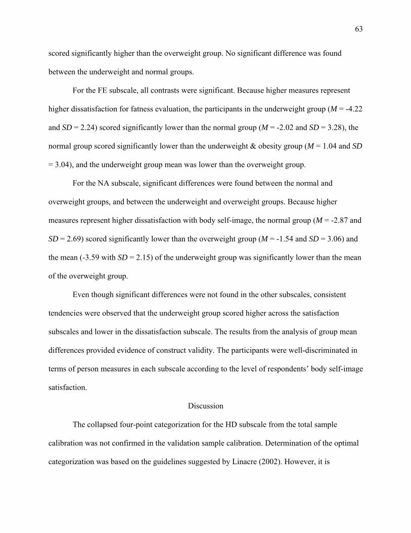
63

scored significantly higher than the overweight group. No significant difference was found

between the underweight and normal groups.

For the FE subscale, all contrasts were significant. Because higher measures represent

higher dissatisfaction for fatness evaluation, the participants in the underweight group (M = -4.22

and SD = 2.24) scored significantly lower than the normal group (M = -2.02 and SD = 3.28), the

normal group scored significantly lower than the underweight & obesity group (M = 1.04 and SD

= 3.04), and the underweight group mean was lower than the overweight group.

For the NA subscale, significant differences were found between the normal and

overweight groups, and between the underweight and overweight groups. Because higher

measures represent higher dissatisfaction with body self-image, the normal group (M = -2.87 and

SD = 2.69) scored significantly lower than the overweight group (M = -1.54 and SD = 3.06) and

the mean (-3.59 with SD = 2.15) of the underweight group was significantly lower than the mean

of the overweight group.

Even though significant differences were not found in the other subscales, consistent

tendencies were observed that the underweight group scored higher across the satisfaction

subscales and lower in the dissatisfaction subscale. The results from the analysis of group mean

differences provided evidence of construct validity. The participants were well-discriminated in

terms of person measures in each subscale according to the level of respondents’ body self-image

satisfaction.

Discussion

The collapsed four-point categorization for the HD subscale from the total sample

calibration was not confirmed in the validation sample calibration. Determination of the optimal

categorization was based on the guidelines suggested by Linacre (2002). However, it is

64

somewhat questionable to collapse categories when the guidelines are applied strictly even

though collapsing categories affects the measurement quality. For example, the original

categorization for the HD subscale was collapsed into a four-point categorization in the total

sample calibration due to the step advance (.96) from the second to third step calibrations, which

was smaller than 1.0 logit. However, the collapsing of categories decreased the person and item

separation statistics from 1.56 (person reliability = .71) and 8.63 (item reliability = .99) to 1.50

(person reliability = .69) and 7.80 (item reliability = .98), respectively. Similar results were

found in the SD and II subscales while collapsing categories for the FE subscale increased

person separation and decreased item separation statistic. Even though it is recommended to

collapse adjacent categories to improve category function in terms of measures and statistics as

suggested in the guidelines (Linacre, 2002), it seems that satisfying the guidelines does not

always improve the psychometric quality of a scale as observed in the present study. Ewing,

Salzberger, and Sinkovics (2005) also suggested that inclusion of other criteria such as

maximizing the item and person separations might alter the decisions made to collapse adjacent

categories. In the present study, all measures and step calibrations were hierarchically ordered

and each category had its own boundary. Therefore, the original categorization may be kept for

the all subscales of the BSIQ instead of employing two different sets of categorization; the

original categorization for certain subscales and the collapsed categorization for the other

subscales.

The Rasch analysis also provided information about misfitting items related to other

latent variables rather than corresponding body image traits. Three misfitting items were detected

by the Rasch analysis and these items were deleted from subsequent analyses. The three items

were items 22 and 35 for the FE subscale and item 11 for the NA subscale. The items were also

65

identified as misfit in the validation sample calibration. Therefore, it is possible that the items are

related to other dimensions not shared by the remaining items. However, misfitting items should

be deleted with a caution especially when the fit statistics for the misfitting items are within a

mean square of 2.0. According to Linacre (2004a) items with fit statistics ranged from 1.5 to 2.0

may be unproductive for construction of measurement but do not degrade the quality of

measurement. Therefore, deleting items depends on the researcher’s purpose of research. In the

present study, for the FE subscale, Infit and Outfit mean squares were 1.72 and 1.80 for item 22,

and 1.42 and 1.55 for item 35. For item 11, Infit and Outfit mean squares were 1.45 and 1.55,

respectively. The fit statistics for these items were very close to the cutoff values except item 22

and one or either statistics was within the range of 1.5 to 2.0 indicating unproductive but no

degrading measurement. Even though the three misfitting items were deleted from the BSIQ

according to the guidelines to demonstrate the application of the Rasch analysis in the present

study, another criteria representing the quality of measurement (e.g., separation statistics) might

be applied and investigated to confirm the decision for deleting misfitting items. In the present

study, deleting two misfitting items from the FE subscale increased both item and person

separation statistics from 19.23 (item reliability = 1.00) and 2.25 (person reliability = .84) to

26.82 (item reliability = 1.00) and 2.35 (person reliability = .85) while deleting item 11 from the

NA subscale decreased both item and person separation statistics from 9.89 (item reliability

= .99) and 1.93 (person reliability = .79) to 7.02 (item reliability = .98) and 1.88 (person

reliability = .78). Therefore, deleting the two misfitting items from the FE subscale seems

reasonable to improve the quality of the BSIQ while deleting item 11 from the NA subscale is

questionable. If it is the case of developing a questionnaire, it is recommended to revise the items

in terms of wording of the statements.

66

The stability of item parameter estimation across the different sample sizes was examined.

Zhu (2002) reported the correlation of item measures generated from two Rasch rating scale

analyses and the rank correlation of the item severity orders to investigate the invariance of the

Rasch estimation. In the present study, however, the correlation of item measures obtained from

the total and validation samples was not estimated due to the relatively small number of items.

Instead, hierarchical order of item measures was compared. Item orders from the two samples

were identical. Small amount of changes in fit statistics and item measures were observed.

However, differences between the two estimations were relatively small or minimal.

Construct validity was conducted to investigate whether the Rasch calibrated measures of

the BSIQ imply the trait of body self-image satisfaction. Significant differences were found in

the OAE, FE, and NA subscales from the ANOVA with alpha level of .05. Consequently, the

group means for the subscales with significant differences were contrasted using the t-test for

two independent groups with alpha level of .02 to examine which groups significantly

differenced. Significant difference between the underweight and normal groups was found in the

FE subscale (p = .00). The differences between the underweight and overweight groups were

significant in the OAE (p = .00), FE (p = .00), and NA (p = .00) subscales. The differences

between the normal and overweight groups were also significant in the OAE (p = .00), FE (p

= .00), and NA (p = .00) subscales. Although it was not a major part of the study, person

measures estimated from the total sample (N = 1021) were also examined based on the same

grouping method using BMI. Significant differences were found in the OAE, FE, HFE, HD, and

NA subscales. In other subscales that didn’t have significant differences among groups,

participants in higher BMI group tended to endorse lower categories in the body self-image

67

satisfaction subscales and higher categories in the dissatisfaction subscales. This additional result

was consistent with the result of the group mean comparisons for the validation sample.

The measurement quality of the BSIQ should be discussed in terms of the variety of item

difficulties and the number of items. The item difficulties were somewhat limited to a small

range. For example, item difficulties for the SD subscale ranged from -.18 to .25 in logits. Since

the range of difficulty is normally from -3.0 to +3.0 (Baker, 1985), the item difficulties for the

SD subscales are very limited. As presented in Figure 10 and seen in Table 8, items cover only a

small part of person abilities that ranged from -4 to +4. Consequently, person separation (1.09)

and reliability (.54) for this subscale were relatively low because the scale items identified

individual differences not as effective as other subscale items such as the FE (person separation

= 2.40 and reliability = .85). The lack of items and the limited item difficulty range also resulted

in many maximal and minimal extreme scores (by respondents who assigned the highest

categories for all items or lowest categories for all items). Even though measures are assigned to

those extreme cases with the estimation process, the accuracy of estimation and the quality of

measurement decrease as the number of extreme cases increases. Therefore, it is recommended

to add more items with various item difficulties to each subscale of the BSIQ to identify

respondents’ ability and individual differences effectively.

For the comparison between the observed scores (i.e., raw scores) and the Rasch

calibrated person measures, there was a strong relationship. For example, the correlation between

the raw scores and the person measures in logits for the OAE subscale was .99. For this reason, it

may be questioned why the Rasch calibrated measures should be used instead of the total scores

(i.e., subscale scores in this study) which is calculated from ordinal scales. The Rasch calibrated

measures do not have any of the fundamental measurement concerns which are the critical issues

68

in the application of CTT to ordinal data. Because the Rasch calibrated measures are statistically

proven to have the characteristics of interval data, it is desirable to use the Rasch measures over

the ordinal data to calculate total or subscale scores. As presented in Figure 15, the relationship

between the raw scores and the person measures in logits is curvilinear. For the raw subscale

scores (i.e., vertical axis in Figure 15), one integer increment from 5 to 6 is the same as the

increment of 1 from 11 to 12. However, the distances between 5 and 6 and 11 and 12 are not

likely to be the same for the person measures in logits (horizontal axis in Figure 15). Therefore,

calculating total scores from ordinal scales may mislead researchers in interpreting the results, so

converting raw scores from an ordinal scale to linear measures using the Rasch analysis is

necessary to compare differences and changes on a linear continuum.

69

Table 5

Rating Scale Model Category Function Statistics for the Original Categorization

Observed Subscale Response

category Count %

Average

measure

Expected

measure

Outfit

MnSq

Step

calibration

Step

advance

1 148 4% -3.16 -3.31 1.28 None

2 667 17% -1.80 -1.71 .91 -3.99 None

3 1358 35% .01 .02 .86 -1.59 2.40

4 1325 34% 2.26 2.17 .94 1.10 2.69

OAE

5 357 9% 3.90 4.07 1.18 4.47 3.37

1 1939 31% -2.31 -2.25 1.07 None

2 1512 24% -.95 -1.05 .84 -1.37 None

3 964 16% -.07 -.13 1.02 -.12 1.25

4 894 14% .59 .69 1.15 .36 .48

FE

5 891 14% 1.61 1.61 1.11 1.14 .78

Missing 2 0% -1.29

1 92 3% -2.71 -2.74 1.02 None

2 464 16% -1.16 -1.12 .92 -3.53 None

3 802 28% .34 .35 .94 -.92 2.61

4 1080 38% 1.95 1.89 .99 .81 1.73

AG

5 427 15% 3.40 3.48 1.08 3.64 2.83

1 505 8% -2.75 -2.69 1.08 None

2 1198 20% -1.48 -1.43 .87 -2.90 None

3 2037 34% -.18 -.20 .80 -1.36 1.54

4 1735 29% 1.45 1.35 1.04 .69 2.05

HFE

5 506 8% 3.11 3.38 1.29 3.56 2.87

Missing 1 0% -2.30

1 134 5% -1.52 -1.85 1.43 None

2 360 13% -.86 -.75 .94 -2.26 None

3 724 26% .21 .30 .90 -.93 1.33

4 902 32% 1.61 1.52 .89 .68 1.61

HFI

5 673 24% 2.93 2.95 1.04 2.51 1.83

70

Table 5 (Continued).


category Count %

Average

measure

Expected

measure

Outfit

MnSq

Step

calibration

Step

advance

1 297 10% -1.44 -1.62 1.22 None

2 768 26% -.83 -.72 .87 -2.11 None

3 744 25% .10 .09 .85 -.27 1.84

4 750 26% .89 .85 .90 .46 .73

SD

5 381 13% 1.64 1.64 1.03 1.92 1.46

1 381 18% -2.45 -2.58 1.26 None

2 658 31% -1.46 -1.34 .83 -2.52 None

3 459 22% -.14 -.14 .76 -.37 2.15

4 403 19% 1.18 751.08 .89 .59 .96

HD

5 229 11% 2.33 2.37 1.22 2.30 1.71

1 1377 34% -3.20 -3.13 .99 None

2 1341 33% -1.68 -1.74 .88 -2.43 None

3 729 18% -.36 -.43 .84 -.46 1.97

4 398 10% .83 .76 1.00 .77 1.23

NA

5 195 5% 1.79 2.11 1.55 2.12 1.35

1 176 4% -.99 -1.33 1.49 None

2 672 14% -.40 -.34 1.01 -2.13 None

3 1028 22% .40 .45 .84 -.36 1.77

4 1632 35% 1.28 1.29 .89 .39 .75

II

5 1221 26% 2.40 2.36 1.01 2.10 1.71

Note. OAE = Overall Appearance Evaluation; FE = Fatness Evaluation; AG = Attention to Grooming; HFE =

Health Fitness Evaluation; HFI = Health Fitness Influence; SD = Social Dependence; HD = Height Dissatisfaction;

NA = Negative Affect; II = Investment in Ideals. MsSq indicates mean square error. If a step advance is larger than

5.0 or smaller than 1.0, the categorization is considered problematic.

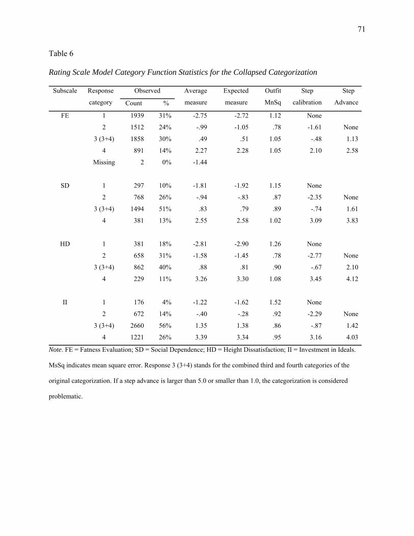
71

Table 6

Rating Scale Model Category Function Statistics for the Collapsed Categorization


category Count %

Average

measure

Expected

measure

Outfit

MnSq

Step

calibration

Step

Advance

1 1939 31% -2.75 -2.72 1.12 None

2 1512 24% -.99 -1.05 .78 -1.61 None

3 (3+4) 1858 30% .49 .51 1.05 -.48 1.13

FE

4 891 14% 2.27 2.28 1.05 2.10 2.58

Missing 2 0% -1.44

1 297 10% -1.81 -1.92 1.15 None

2 768 26% -.94 -.83 .87 -2.35 None

3 (3+4) 1494 51% .83 .79 .89 -.74 1.61

SD

4 381 13% 2.55 2.58 1.02 3.09 3.83

1 381 18% -2.81 -2.90 1.26 None

2 658 31% -1.58 -1.45 .78 -2.77 None

3 (3+4) 862 40% .88 .81 .90 -.67 2.10

HD

4 229 11% 3.26 3.30 1.08 3.45 4.12

1 176 4% -1.22 -1.62 1.52 None

2 672 14% -.40 -.28 .92 -2.29 None

3 (3+4) 2660 56% 1.35 1.38 .86 -.87 1.42

II

4 1221 26% 3.39 3.34 .95 3.16 4.03

Note. FE = Fatness Evaluation; SD = Social Dependence; HD = Height Dissatisfaction; II = Investment in Ideals.

MsSq indicates mean square error. Response 3 (3+4) stands for the combined third and fourth categories of the

original categorization. If a step advance is larger than 5.0 or smaller than 1.0, the categorization is considered

problematic.

72

Table 7

Rating Scale Model Category Function Statistics for the Fatness Evaluation (FE) Subscale with

the Collapsed Categorization after the Deletion of Items 22 and 35


category Count %

Average

measure

Expected

measure

Outfit

MnSq

Step

calibration

Step

Advance

1 1335 32% -4.17 -4.15 .99 None

2 1052 25% -1.46 -1.47 .79 -2.49 None

3 (3+4) 1220 29% .96 .89 1.17 -.47 2.02

FE

4 598 14% 3.60 3.68 1.08 2.96 3.43

Note. MsSq indicates mean square error. Response 3 (3+4) stands for the combined third and fourth categories of the

original categorization. If a step advance is larger than 5.0 or smaller than 1.0, the categorization is considered

problematic.

73

Table 8

Rating Scale Model Item Fit Statistics for the Retained Items with the Optimal Categorization in

Each Subscale

Subscale Item

Number Item

Raw

score Count Measure Error Infit Outfit

I10 Naked body OK 3220 964 -.18 .06 1.35 1.35

I17 Good in clothes 3330 964 -.52 .06 .94 .93

I26 Body looks good 3004 964 .48 .05 .71 .71

OAE

I32 Sexually appealing 3087 963 .22 .06 .96 .95

I07 Looks fat in clothes 1624 841 1.10 .07 .85 .87

I14 Partly fat 2470 841 -2.38 .06 1.02 1.11

I18 Fat overall 1387 841 2.23 .07 .99 1.02

I29 Overweight 1683 841 .84 .07 .88 .81

FE

I39 Wish thinner 2327 841 -1.79 .06 1.15 1.10

I06 Attention to face & hair 3435 955 -.37 .05 .77 .76

I12 Usually well dressed 3390 955 -.25 .05 1.18 1.20

AG

I20 Time to be attractive 3056 955 .62 .05 1.01 1.00

I03 Overall fit high 2928 997 .36 .05 .92 .95

I13 Body is healthy 3557 997 -1.13 .05 1.09 1.12

I21 Muscle tone good 2905 996 .41 .05 .76 .77

I28 Body is strong 3231 997 -.34 .05 1.05 1.05

I34 Athletic build 2831 997 .58 .05 1.37 1.34

HFE

I37 Body in shape 3030 997 .13 .05 .71 .72

I23 Body function 3124 931 .51 .04 .93 .94

I30 Exercise regularly 3959 931 -1.42 .05 1.28 1.20

HFI

I36 State of my health 2916 931 .91 .04 .86 .85

I04 Clothes dependence 2532 980 .25 .05 1.00 .99

I08 Comparing to people 2671 980 -.18 .06 1.07 1.04

SD

I15 Social awareness 2636 980 -.07 .06 .93 .90

74


Subscale Item

number Item

Raw

score Count Measure Error Infit Outfit

I02 Want to be taller 1872 710 -.64 .07 1.16 1.15

I25 Different height 1751 710 -.08 .07 .72 .69

HD

I38 Different HT better 1576 710 .72 .07 1.12 1.13

I05 Naked body sad 1668 677 -.52 .06 .98 .97

I19 Naked body angry 1342 677 .69 .06 1.22 1.08

I27 Depressed about body 1514 677 .02 .06 .87 .85

NA

I33 Feel bad about body 1575 677 -.20 .06 .97 .98

I01 Control fat level 2863 946 .07 .06 1.16 1.15

I09 Well proportioned body 3024 946 -.58 .07 .74 .70

I16 Muscle definition 2720 946 .59 .06 1.09 1.12

I24 Legs shaped 2817 946 .24 .06 1.02 1.00

II

I31 Size matters 2960 945 -.32 .06 .98 .95

Note. OAE = Overall Appearance Evaluation; FE = Fatness Evaluation; AG = Attention to Grooming; HFE =

Health Fitness Evaluation; HFI = Health Fitness Influence; SD = Social Dependence; HD = Height Dissatisfaction;

NA = Negative Affect; II = Investment in Ideals.

75

Table 9

One-Way Analysis of Variance for the Person Body Self-Image Measures Among the Three Body

Mass Index (BMI) Groups

Subscale Source df F p

Between groups 2 14.573* .000

Within groups 500

Overall appearance evaluation

Total 502


Within groups 500

Fatness evaluation

Total 502

Between groups 2 2.573 .077

Within groups 500

Attention to grooming

Total 502


Within groups 500

Health fitness evaluation

Total 502

Between groups 2 .480 .619

Within groups 500

Health fitness influence

Total 502


Within groups 500

Social dependence

Total 502


Within groups 500

Height dissatisfaction

Total 502


Within groups 500

Negative affect

Total 502

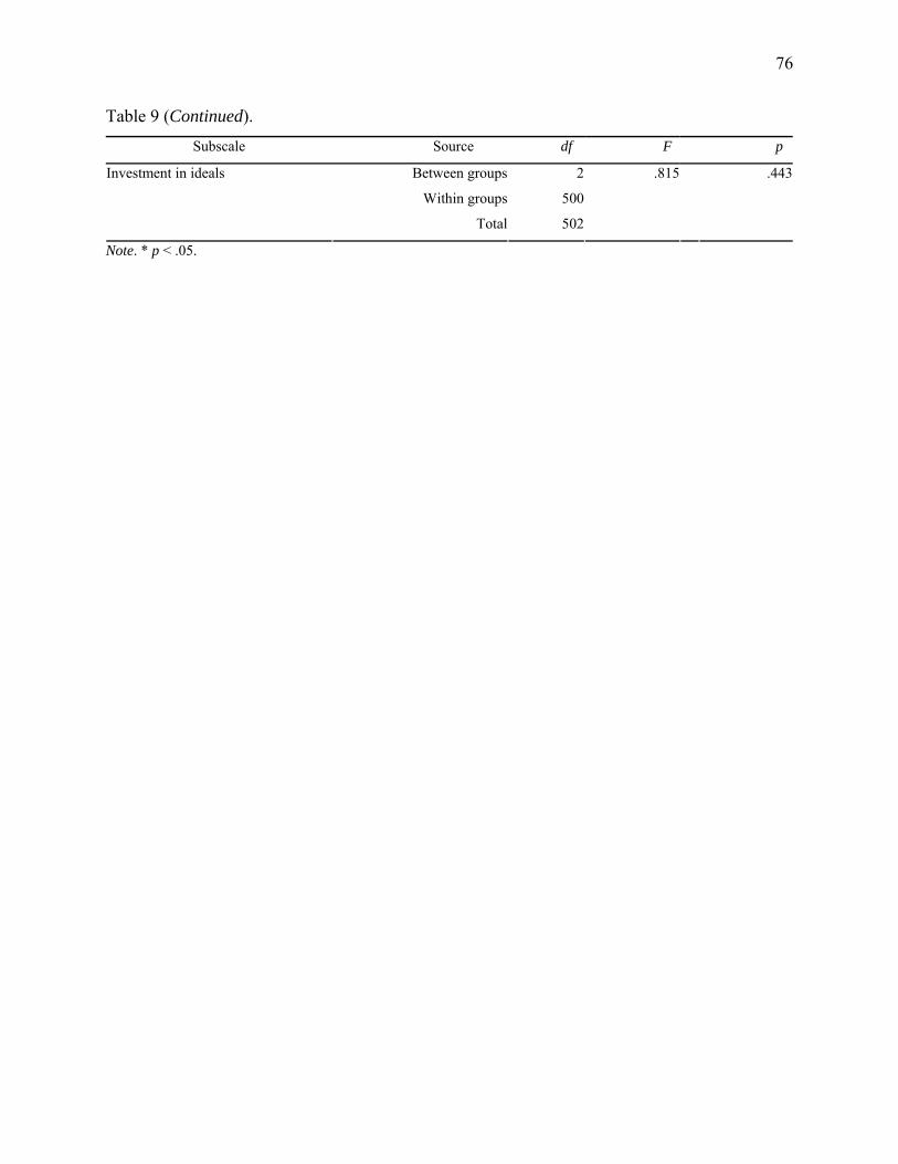
76


Subscale Source df F p


Within groups 500

Investment in ideals

Total 502

Note. * p < .05.

77

Table 10

Contrast (t-test) Among the Three Body Mass Index (BMI) Groups

Subscale Contrast Std. Error df t p

1 .4907 41.165 1.483 .146

2 .3096 153.867 4.740* .000

Overall appearance evaluation

3 .5468 60.975 4.015* .000

1 .4139 50.882 -5.323* .000

2 .3464 172.599 -8.830* .000

Fatness evaluation

3 .4819 82.293 -10.919* .000

1 .4937 40.169 1.601 .117

2 .2489 179.481 1.094 .275

Attention to grooming

3 .5226 49.775 2.033 .047

1 .4779 39.231 -.114 .909

2 .2558 153.028 1.979 .050

Health fitness evaluation

3 .5181 53.114 .872 .387

1 .3628 39.791 -.669 .508

2 .1840 171.103 -.475 .636

Health fitness influence

3 .3861 50.302 -.855 .397

1 .4130 40.481 .045 .964

2 .2256 168.538 -.820 .413

Social dependence

3 .4443 53.171 -.375 .709

1 .4681 44.815 -.288 .775

2 .3449 160.746 -2.165 .032

Height dissatisfaction

3 .5356 71.174 -1.646 .104

1 .3843 46.624 -1.871 .068

2 .3340 147.641 -3.979* .000

Negative affect

3 .4685 87.577 -4.371* .000

78


Subscale Contrast Std. Error df t p

1 .4419 39.872 .325 .747

2 .2328 165.454 1.189 .236

Investment in ideals

3 .4740 51.908 .887 .379

Note. Equal variances were not assumed. Contrast 1 = underweight group vs. overweight group; contrast 2 =

underweight group vs. normal group; contrast 3 = normal group vs. overweight group. * p < .02.

79

SD Original Categorization

Person Location (Bn - Di)

-5 -4 -3 -2 -1 0 1 2 3 4 5

Prob

abili

ty o

f Obs

erva

tion

0.0

0.1

0.2

0.3

0.4

0.5

0.6

0.7

0.8

0.9

1.0 Category 1

Category 2Category 3

Category 4

Category 5

SD Collapsed Categorization


-5 -4 -3 -2 -1 0 1 2 3 4 5 6

Prob

abili

ty o

f Obs

erva

tion

0.0

0.1

0.2

0.3

0.4

0.5

0.6

0.7

0.8

0.9

1.0Category 1

Category 2

Category 3(3+4)

Category 4

Figure 1. Rating scale model category probability curves for the original and collapsed

categorizations for the social dependence (SD) subscale.

80

HD Original Categorization


-5 -4 -3 -2 -1 0 1 2 3 4 5

Prob

abili

ty o

f Obs

erva

tion

0.0

0.1

0.2

0.3

0.4

0.5

0.6

0.7

0.8

0.9

1.0Category 1

Category 2


Category 5

HD Collapsed Categorization


-5 -4 -3 -2 -1 0 1 2 3 4 5 6

Prob

abili

ty o

f Obs

erva

tion

0.0

0.1

0.2

0.3

0.4

0.5

0.6

0.7

0.8

0.9

1.0Category 1

Category 2

Category 3(3+4)

Category 4


categorizations for the height dissatisfaction (HD) subscale.

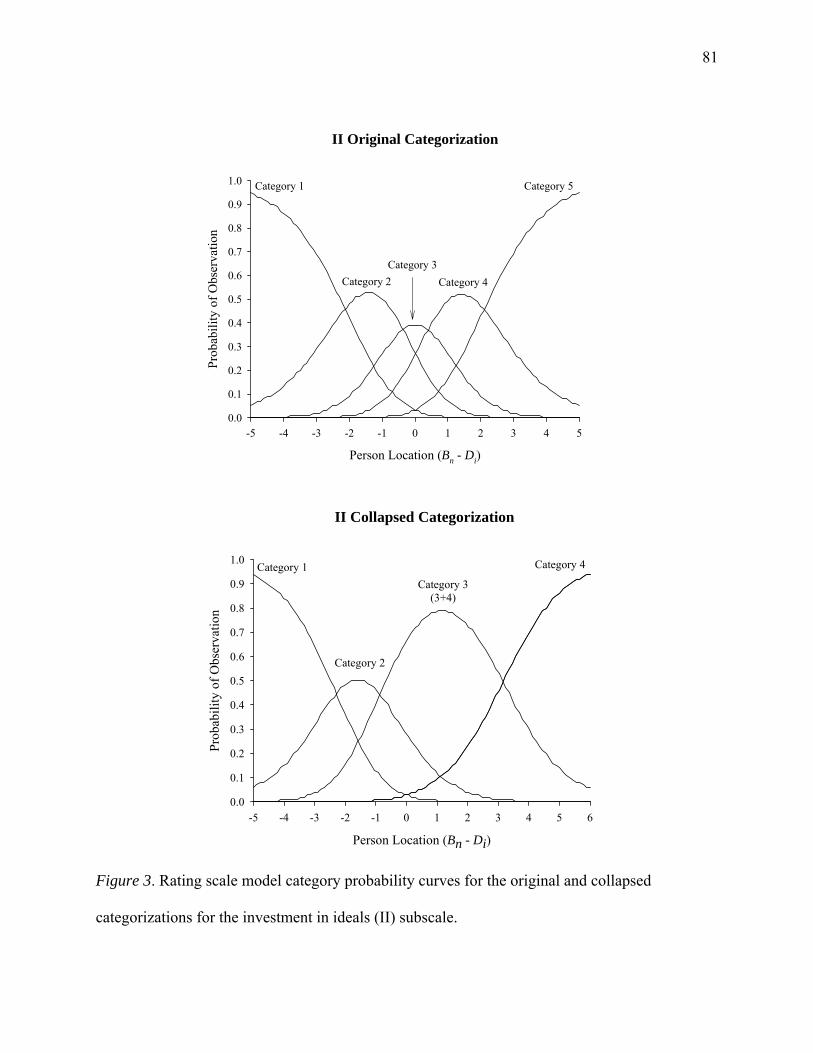
81

II Original Categorization


-5 -4 -3 -2 -1 0 1 2 3 4 5

Prob

abili

ty o

f Obs

erva

tion

0.0

0.1

0.2

0.3

0.4

0.5

0.6

0.7

0.8

0.9

1.0 Category 1


Category 4

Category 5

II Collapsed Categorization


-5 -4 -3 -2 -1 0 1 2 3 4 5 6

Prob

abili

ty o

f Obs

erva

tion

0.0

0.1

0.2

0.3

0.4

0.5

0.6

0.7

0.8

0.9

1.0 Category 1

Category 2

Category 3(3+4)

Category 4


categorizations for the investment in ideals (II) subscale.

82

FE Original Categorization


-4 -3 -2 -1 0 1 2 3 4

Prob

abili

ty o

f Obs

erva

tion

0.0

0.1

0.2

0.3

0.4

0.5

0.6

0.7

0.8

0.9

1.0Category 1

Category 2

Category 3

Category 4

Category 5

FE Collapsed Categorization


-5 -4 -3 -2 -1 0 1 2 3 4 5 6

Prob

abili

ty o

f Obs

erva

tion

0.0

0.1

0.2

0.3

0.4

0.5

0.6

0.7

0.8

0.9

1.0Category 1

Category 2

Category 3(3+4)

Category 4


categorizations for the fatness evaluation (FE) subscale after the deletion of the items 22 and 35.

83

Measure Person Item

<more>|<rare> 6 .#### + | .## | T| . | 5 + # 10 Respondents | M Mean

.#### | S 1 Standard Deviation | T 2 Standard Deviation | 4 + | .####### | | | 3 S+ .########## | | | | 2 .########### + | | | .######## | 1 +

M|T | .########## |S I26: Body looks good | I32: Sexually appealing 0 +M

I10: Naked body OK ########### | |S | I17: Good in clothes .######## |T -1 + | | .####### S| | -2 + ###### | | | .### | -3 + | .# | | | -4 T+ . | | | | -5 + . | | | | -6 .# + <less>|<frequ>

Figure 5. Map for the person and item parameter estimates for the overall appearance evaluation

(OAE) subscale.

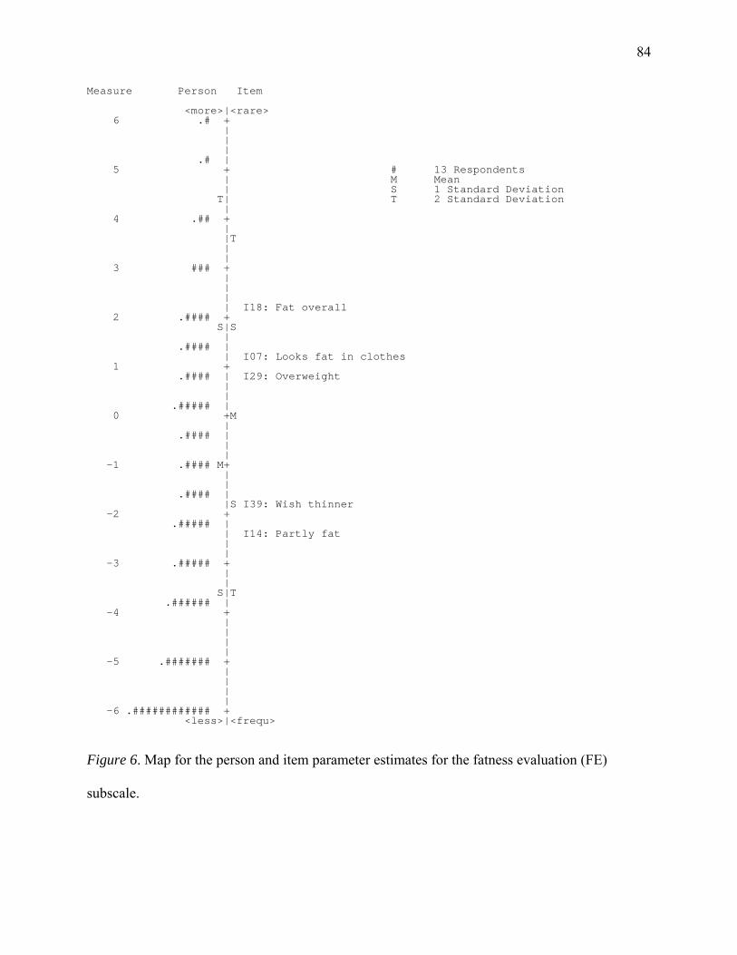
84

Measure Person Item <more>|<rare> 6 .# + | | | .# | 5 + # 13 Respondents | M Mean

| S 1 Standard Deviation T 2 Standard Deviation T|

| 4 .## + | |T | | 3 ### + | | | | I18: Fat overall 2 .#### +

S|S | .#### | | I07: Looks fat in clothes 1 +

I29: Overweight .#### | | | .##### | 0 +M | .#### | | | -1 .#### M+ | | .#### |

I39: Wish thinner |S -2 + .##### | | I14: Partly fat | | -3 .##### + | | S|T .###### | -4 + | | | | -5 .####### + | | | | -6 .############ + <less>|<frequ>

Figure 6. Map for the person and item parameter estimates for the fatness evaluation (FE)

subscale.

85

Measure Person Item

<more>|<rare> 5 ##### T+ | | .####### | | |

spondents 4 + # 12 Re | M Mean | S 1 Standard Deviation | T 2 Standard Deviation .######## | | 3 S+ | | | .############ | | 2 + | | | .############ | | 1 M+ |T

I20: Time to be attractive .########## | |S | | 0 .######### +M | I12: Usually well dressed

I06: Attention to face & hair | |S .###### | S|T -1 + | | .###### | | | -2 + | .## | | | T| -3 + .# | | | | | -4 + | . | | | | -5 . + <less>|<frequ>

Figure 7. Map for the person and item parameter estimates for the attention to grooming (AG)

subscale.

86

Measure Person Item

<more>|<rare> 6 ### + | | .# | | 5 + # 7 Respondents | M Mean | S 1 Standard Deviation .### | T 2 Standard Deviation | 4 T+ .### | | | .### | 3 + | #### | | .####### | 2 S+ | .######## | | .######### |T 1 + .######## | |S I34: Athletic build .########## | I21: Muscle tone good I03: Overall fit high | I37: Body in shape 0 .########### M+M .########### |

I28: Body is strong | .####### |S | -1 .########## + .######### |T I13: Body is healthy | .####### | .####### S| -2 + .#### | | .### | | -3 ### + | .## | | T| -4 .# + | | | .# | -5 . + <less>|<frequ>

Figure 8. Map for the person and item parameter estimates for the health fitness evaluation

(HFE) subscale.

87

Measure Person Item

<more>|<rare> 4 .###### T+ | .###### | | | |

spondents 3 + # 13 Re | M Mean | S 1 Standard Deviation .########## S| T 2 Standard Deviation | |

2 +T .########### | | | | ############# M| 1 +S

I36: State of my health | | .########## | I23: Body functioning | | 0 .####### +M | S| | .##### | | -1 +S .### | | | I30: Exercise Regularly | .# T| -2 +T | | . | | | -3 + | | . | | | -4 + | | | | | -5 . + <less>|<frequ>

Figure 9. Map for the person and item parameter estimates for the health fitness influence (HFI)

subscale.

88

Measure Person Item

<more>|<rare> 4 # + .### T| | | | | |

spondents 3 + # 18 Re | M Mean | S 1 Standard Deviation .####### | T 2 Standard Deviation | | S| 2 + | | | | | .############ | 1 + | | | |T

I04: Clothes dependence M| |S 0 .########## +M I15: Social awareness |S I08: Comparing to people |

|T | | .######## | -1 + | | S| .###### | | | -2 + | .### | | | | | -3 + | .# T| | | | | -4 .# + <less>|<frequ>

Figure 10. Map for the person and item parameter estimates for the social dependence (SD)

subscale.

89

Measure Person Item

<more>|<rare> 5 #### + | | | T| .### |

spondents 4 + # 19 Re | M Mean | S 1 Standard Deviation | T 2 Standard Deviation | | 3 + .## | | | | | 2 S+ | | | .###### | |T 1 + |

I38: Different HT better | |S | .##### | 0 +M I25: Wish Different height | M| |S | I02: Want to be taller .##### | -1 +

|T | | .###### | | -2 + | | S| .#### | | -3 + | | | .#### | | -4 .############ + <less>|<frequ>

Figure 11. Map for the person and item parameter estimates for the height dissatisfaction (HD)

subscale.

90

Measure Person Item

<more>|<rare> 4 . + . | | | | |

spondents 3 . + # 26 Re | M Mean | S 1 Standard Deviation T| T 2 Standard Deviation . | | 2 + . | | | . | | 1 . + |T . | I19: Naked body angry S|S | .# |

0 +M I27: Depressed about body I33: Feel bad about body |

## | |S I05: Naked body sad .# | |T -1 + .## | | M| | .## | -2 + | | .## | | | -3 + .### | | S| | | -4 + .#### | | | | | -5 .############ + <less>|<frequ>

Figure 12. Map for the person and item parameter estimates for the negative affect (NA)

subscale.

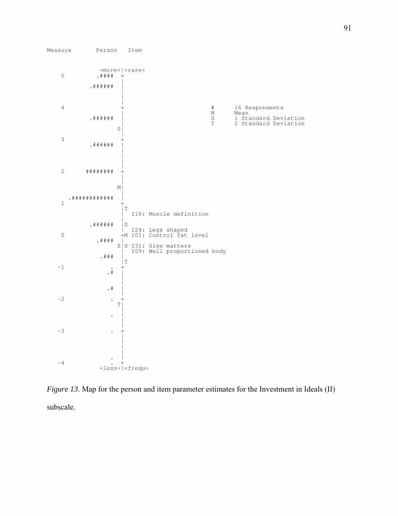
91

Measure Person Item

<more>|<rare> 5 .#### + | .###### | | | |

pondents 4 + # 16 Res | M Mean .###### | S 1 Standard Deviation | T 2 Standard Deviation S| | 3 + .###### | | | | | 2 ######## + | | M| | .############ | 1 + |T

I16: Muscle definition | | .###### |S | I24: Legs shaped 0 +M I01: Control fat level .#### | S|S I31: Size matters | I09: Well proportioned body .### | |T -1 . + .# | | | .# | | -2 . + T| | . | | | -3 . + | | | | . | -4 . + <less>|<frequ>

Figure 13. Map for the person and item parameter estimates for the Investment in Ideals (II)

subscale.

92

Total Sample (N = 1021)

-3 -2 -1 0 1 2 3

Val

idat

ion

Sam

ple

(n =

510

)

-3

-2

-1

0

1

2

3

Figure 14. Differential item functioning of the Body Self-Image Questionnaire (BSIQ) in the

total sample and the validation sample. The slope of the regression line is 1.0 and the unit of the

measures is logits.

93

Person Measure (Bn)-6 -5 -4 -3 -2 -1 0 1 2 3 4 5 6 7

Raw

Sub

scal

e Sc

ore

SCORE456789

1011121314151617181920

Figure 15. Curvilinear relationship between the raw scores and the Rasch calibrated person

measures for the Overall Appearance Evaluation (OAE) subscale.

94

CHAPTER 5

SUMMARY AND CONCLUSSIONS

The present study was designed to evaluate the application of the Rasch analysis to

converting ordinal data into interval data, to optimizing the number of categories, and to

constructing items for each subscales of the BSIQ. The data from 1021 undergraduate students

were used in this study. The analysis was conducted on each of the nine subscales of the BSIQ.

Summary

The Rasch analysis using the RSM provided information concerning determining the

optimal categorization for the subscales of the BSIQ. From the series of RSM calibrations, the

four-point categorization was found appropriate for the FE, SD, HD, and II subscales and the

original five-point categorization was retained for the other subscales. The collapsed

categorization and the original categorization determined in the total sample calibration were

confirmed in the validation sample calibration except for the categorization for the HD subscale.

The different result for the HD subscale have resulted from the different category endorsement

patterns across the samples. Even though the validation sample was drawn randomly from the

total sample, the endorsement pattern may not be controlled.

The Rasch analysis detected misfitting items in the total sample and validation sample

calibrations. The misfitting items may be related to other latent variables rather than the body

self-image trait. Even though the misfitting items were deleted from subsequent analyses to

demonstrate the application of the Rasch analysis strictly according to the guidelines, the results

95

can be used for reconstructing items for a scale in a different way. Because only numerical and

empirical aspects of item fit were examined in this study, linguistic aspects of items such as the

choice of relevant words and clarity of statements should be examined and revised before

deleting misfitting items especially when developing a scale or a questionnaire.

Item and person parameter estimates for each subscale were obtained from the final

calibration for the total sample after optimizing categorization and deleting misfitting items. The

estimates were linear measures which were converted from observed scores obtained from an

ordinal scale. Therefore, comparing item difficulties and person abilities (i.e., body self-image

satisfaction and dissatisfaction) on the same yardstick without linearity concerns was

demonstrated.

The optimal categorization and structure of items for each subscale of the BSIQ were

cross-validated using the validation sample. In general, the patterns of categorization perceived

by participants were consistent across the samples. Item parameter estimations across the

samples were also stable and the hierarchical order of item difficulties was identical in both

samples. Similar findings, the invariance feature of the Rasch analysis in estimating parameter

measures, have been reported (Ewing et al., 2005; Zhu, 2002).

Evidence of construct validity using the Rasch calibrated person measures were provided.

The mean person measures in logits for three BMI-based groups were compared for each

subscale and contrasted to examine which groups significantly differenced. Generally,

participants in higher BMI group tended to endorse lower categories in the body self-image

satisfaction subscales and higher categories in the dissatisfaction subscales and vice versa.

96

Conclusions

Based on the findings from this study, two major conclusions can be drawn. The RSM

provided advantages such as an effective and objective way to examine the categorization of the

BSIQ and a solution to reduce linearity concerns by transforming ordinal data into logits. In

regard to the research questions in the present study:

1. The BSIQ data fit the RSM in terms of fit statistics.

2. The RSM calibration adequately contrasts items and participants respectively according

to their measures in logits.

3. The response categorization of the BSIQ is functioning as intended except for the FE, SD,

HD, and II subscales. Combining the third and fourth categories results in the most

acceptable fits for the FE, SD, and II subscales.

4. The Rasch categorization and item structure are stable and consistent across the samples.

97

REFERENCES

American College of Sports Medicine. (2000). ACSM’s guidelines for exercise testing and

prescription (6th ed.). Baltimore: Williams & Wilkins.

Andersen, E. B. (1973). A goodness of fit test for the Rasch model. Psychometrika, 38, 123-140.

Andersen, E. B. (1977). Sufficient statistics and latent trait models. Psychometrika, 42, 69-81.

Andrich, D. (1978). A rating formulation for ordered response categories. Psychometrika, 43,

561-573.

Andrich, D. (1988). Rasch models for measurement. Newberry Park, CA: Sage.

Andrich, D. (1996). Measurement criteria for choosing among models with graded responses. In

A. Von Eye & C. C. Clogg (Eds.), Categorical variables in developmental research:

Methods of analysis (pp. 3-35). Orlando, FL: Academic Press.

Andrich, D. (1997). Rating scale analysis. In J. P. Keeves (Ed.), Educational research,

methodology, and measurement: An international handbook (2nd ed., pp. 874-880). New

York: Elsevier.

Angoff, W. H. (1960). Measurement and scaling. In C. W. Harris (Ed.), Encyclopedia of

educational research (3rd ed., pp. 807-817). New York: Macmillan.

Askevold, R. (1975). Measuring body image: Preliminary report on a new method.

Psychotherapy and Psychosomatics, 26, 71-77.

Baker, F. B. (1985). The basics of item response theory. Portsmouth, NH: Heinemann.

98

Baker, F. B. (1992). Item Response theory: Parameter estimation techniques. New York: Marcel

Dekker.

Baumgartner, T. A., Jackson, A. S., Mahar, M. T., & Rowe, D. A. (2003). Measurement for

evaluation in physical education & exercise Science (7th ed.). New York: McGraw-Hill.

Benson, J., & Nasser, F. (1998). On the use of factor analysis as a research tool. Journal of

Vocational Education Research, 23, 13-33.

Birnbaum, A. (1968). Some latent trait models and their use in inferring an examinee’s ability. In

F. M. Lord, & M. R. Novick, Statistical theories of mental test scores. Reading, MA:

Addison-Wesley.

Bond, T. G., & Fox, C. M. (2001). Applying the Rasch model: Fundamental measurement in the

human sciences. Mahwah, NJ: Lawrence Erlbaum.

Brown, T., Cash, T., & Lewis, R. (1989). Body-image disturbances in adolescent female binge-

purgers: A brief report of a national survey in the USA. Journal of Child Psychology and

Psychiatry, 30, 605-613.

Cash, T. F. (1990). The Multidimensional Body-Self Relations Questionnaire. Unpublished

manuscript, Old Dominion University, Norfolk, VA.

Cash, T. F., Winstead, B. A., & Janda, L. H. (1986). Body image survey report: The great

American shape-up. Psychology Today, 24, 30-37.

Chang, S. T. (1985). Characteristics of anchor tests, person fit, and item calibration with the

Rasch model (doctoral dissertation). Athens: University of Georgia.

Clark, H. H., & Schober, M. F. (1992). Asking questions and influencing answers. In J. M. Tanur

(Ed.), Questions about questions: Inquiries into the cognitive bases of surveys (pp. 15-48).

New York: Russell Sage.

99

Crocker, L., & Algina, J. (1986). Introduction to classical and modern test theory. New York:

Holt, Rhinehart & Winston.

Crocker, L., Llabre, M., & Miller, M. D. (1988). The generalizability of content validity ratings.

Journal of Educational Measurement, 25, 287-299.

Dunbar, S. B., Koretz, D. M., & Hoover, H. D. (1991). Quality control in the development and

use of performance assessment. Applied Measurement in Education, 4, 289-303.

Embretson, S. E. (1999). Issues in the measurement of cognitive abilities. In S. E. Embretson &

S. L. Hershberger (Eds.). The new rules of measurement: What every psychologist and

educator should know (pp. 1-15). Mahwah, NJ: Lawrence Erlbaum.

Embretson, S. E., & Reise, S. P. (2000). Item response theory for psychologists. Mahwah, NJ:

Lawrence Erlbaum.

Ennis, C. D., & Hooper, L. M. (1988). Development of an instrument for assessing educational

value orientations. Journal of Curriculum Studies, 20, 277-280.

Ewing, M. T., Salzberger, T., & Sinkovics, R. R. (2005). An alternative approach to assessing

cross-cultural measurement equivalence in advertising research. Journal of Advertising,

34, 17-36.

Fichter, M. M., & Quadflieg, N. (2003). Predicting the outcome of eating disorders using

structural equation modeling. International Journal of Eating Disorders, 34, 292-313.

Freeman, R. J., Thomas, C. D., Solyom, L., & Hunter, M. A. (1984). A modified video camera

for measuring body image distortion: Technical description and reliability. Psychological

Medicine, 14, 411-416.

Garner, D. M. (1991). Eating Disorder Inventory-2 manual. Odessa, FL: Psychological

Assessment Resources.

100

Garner, D. M., Olmstead, M. A., & Polivy, J. (1983). Development and validation of a

multidimensional eating disorder inventory for anorexia nervosa and bulimia.

International Journal of Eating Disorders, 2, 15-34.

Godin, G., Jobin, J., & Bouillon, J. (1986). Assessment of leisure time exercise behavior by self-

report: A concurrent validity study. Canadian Journal of Public Health, 77, 359-361.

Guilford, J. P. (1954). Psychometric methods (2nd ed.). New York: McGraw-Hill.

Gulliksen, H. (1950). Theory of mental tests. New York: Wiley.

Haley, D. C. (1952). Estimation of the dosage mortality when the dose is subject to error.

(Technical Report, No. 15). Stanford, CA: Stanford University, Applied Mathematics and

Statistics Laboratory.

Hambleton, R. K. (1985). Item response theory. Hingham, MA: Kluwer-Nijhoff.

Hands, B., & Larkin, D. (2001). Using the Rasch measurement model to investigate the construct

of motor ability in young children. Journal of Applied Measurement, 2, 101-120.

Hansen, H., & Gauthier, R. (1989). Factors affecting attendance at professional sport events.

Journal of Sport Management, 3, 15-32.

Hausenblas, H. A., & Fallon, E. A. (2002). Relationship among body image, exercise behavior,

and exercise dependence symptoms. International Journal of Eating Disorders, 32, 179-

185.

Hausenblas, H. A., & Symons Downs, D. (2001). The Exercise Dependence Scale manual.

Unpublished manuscript, University of Florida, Gainesville.

Ingledew, D. K., & Sullivan, G. (2002). Effects of body mass and body image on exercise

motives in adolescence. Psychology of Sport and Exercise, 3, 323-338.

101

Keppel, G. (1991). Design and analysis: A researcher’s handbook (3rd ed.). Upper Saddle River,

NJ: Prentice-Hall.

Kirby, R. L., Swuste, J., Dupuis, D. J., MacLeod, D. A., & Monroe, R. (2002). The wheelchair

skills test: A pilot study of a new outcome measure. Archives of Physical Medicine and

Rehabilitation, 83, 10-18.

Klockars, A. J., & Yamagishi, M. (1988). The influence of labels and positions in rating scales.

Journal of Educational Measurement, 25, 85-96.

Kulinna, P. H., & Zhu, W. (2001). Fitness portfolio calibration for first- through sixth-grade

children. Research Quarterly for Exercise Science and Sport, 72, 324-334.

Kulinna, P. H., Cothran, D., & Regualos, R. (2003). Development of an instrument to measure

student disruptive behavior. Measurement in Physical Education and Exercise Science, 7,

25-41.

Kurtz, R. M. (1969). Sex differences and variations in body attitudes. Journal of Consulting and

Clinical Psychology, 33, 625-629.

Lazarsfeld, P. F., & Henry, N. W. (1968). Latent structure analysis. New York: Houghton

Mifflin.

Likert, R. (1932). A technique for the measurement of attitudes. Archives of Psychology, 140. 1-

55.

Linacre, J. M. (1995). Categorical misfit statistics. Rasch Measurement Transactions, 9, 450-451.

Linacre, J. M. (2002). Optimizing rating scale category effectiveness. Journal of Applied

Measurement, 3, 85-106.

Linacre, J. M. (2004a). A user’s guide to WINSTEPS MINSTEP: Rasch-model computer

programs. Chicago: Winsteps.com.

102

Linacre, J.M. (2004b). WINSTEPS Rasch measurement computer program. Chicago:

Winsteps.com.

Linacre, J. M., & Wright, B. D. (1999). A user’s guide to WINSTEPS BIGSTEPS MINISTEP:

Rasch-model computer programs. Chicago: MESA Press.

Loevinger, J. (1947). A systematic approach to the construction and evaluation of tests of ability.

Psychological Monographs, 61(4).

Looney, M. A. (1997). Objective measurement of figure skating performance. Journal of

Outcome Measurement, 1, 143-163.

Looney, M. A., & Rimmer, J. H. (2003). Aerobic exercise equipment preferences among older

adults: A preliminary investigation. Journal of Applied Measurement, 4, 43-58.

Lord, F. M. (1952). A theory of test scores (Psychometric Monograph No. 7). Psychometric

Society.

Ludlow, L. H., & Haley, S. M. (1995). Rasch model logits: Interpretation, use, and

transformation. Educational Psychological Measurement, 55, 967-975.

Martin, K. A., Rejeski, W. J., Leary, M. R., McAuley, E., & Bain, S. (1997). Is the Social

Physique Anxiety Scale really multidimensional? Conceptual and statistical arguments

for a unidimensional model. Journal of Sport and Exercise Psychology, 19, 359-367.

Masters, G. N. (1982). A Rasch model for partial credit scoring. Psychometrika, 47, 149-174.

Masters, G. N., & Wright, B. D. (1984). The essential process in a family of measurement

models. Psychometrika, 49, 529-544.

Merbitz, C., Morris, J., & Grip, J. C. (1989). Ordinal scales and foundations of misinference.

Archives of Physical Medicine and Rehabilitation, 70, 308-312.

103

Parducci, A., & Wedell, D. H. (1986). The category effect with rating scales: Number of

categories, number of stimuli, and method of presentation. Journal of Experimental

Psychology: Human Perception and Performance, 12, 496-516.

Pietrobelli, A., Faith, M. S., Allison, D. B., Gallagher, D., Chiumello, G., & Heymsfield, S. B.

(1998). Body mass index as a measure of adiposity among children and adolescents: A

validation study. Journal of Pediatrics, 132, 204-210.

Rasch, G. (1960). Probabilistic models for some intelligence and attainment tests. Copenhagen:

Danish Institute for Educational Research.

Rasch, G. (1980). Probabilistic models for some intelligence and attainment tests (with forward

and afterward by B. D. Wright). Chicago: University of Chicago Press.

Roberts, J. (1994). Rating scale functioning. Rasch Measurement Transactions, 8, 386.

Rowe, D. A. (1996). Development and validation of a questionnaire to measure body image

(doctoral dissertation). Athens: University of Georgia.

Rowe, D. A., Benson, J., & Baumgartner, T. A. (1999). Development of the body self-image

questionnaire. Measurement in Physical Education and Exercise Science, 3, 223-247.

Ruff, G. A., & Barrios, B. A. (1986). Realistic assessment of body image. Behavioral

Assessment, 8, 237-252.

Slade, P. D., & Russell, G. F. M. (1973). Awareness of body dimensions in anorexia nervosa:

Corss-sectional and longitudinal studies. Psychological Medicine, 3, 188-199.

Smolak, L. (2002). Body image development in children. In T. F. Cash & T. Pruzinsky (Eds.),

Body image: A handbook of theory, research, and clinical practice (pp. 65-73). New

York: Guilford Press.

104

Smith, Jr., E. V., & Dupeyrat, C. (2001). Toward establishing a unified metric for performance

and learning goal orientations. Journal of Applied Measurement, 2, 312-336.

Stevens, S. S. (1946). On the theory of scales of measurement. Science, 103, 677-680.

Stice, E., Maxfield, J., & Wells, T. (2003). Adverse effects of social pressure to be thin on young

women: An experimental investigation of the effects of “fat talk”. International Journal

of Eating Disorders, 34, 108-117.

Thompson, J. K. (Ed.). (1996). Body image, eating disorders, and obesity: An integrative guide

for assessment and treatment. Washington, DC: American Psychological Association.

Thorndike, E. L. (1926). Educational psychology. New York: Columbia University, Teachers

College.

Thurstone, L. L. (1925). A method of scaling psychological and educational tests. Journal of

Educational Psychology, 16, 433-451.

Thurstone, L. L. (1927). The unit of measurement in educational scales. Journal of Educational

Psychology, 18, 505-524.

Togerson, W. S. (1958). Theory and methods of scaling. New York: John Wiley.

Waugh, R. F. (2003). Measuring attitudes and behaviors to studying and learning for university

students: A Rasch measurement model analysis. Journal of Applied Measurement, 4,

164-180.

Wedell, D. H., Parducci, A., & Lane, M. (1990). Reducing the dependence of clinical judgment

on the immediate context: Effects of number of categories and type of anchors. Journal

of Personality and Social Psychology, 58, 319-329.

105

Williamson, D. A., Cubic, B. A., & Gleaves, D. H. (1993). Equivalence of body image

disturbances in anorexia and bulimia nervosa. Journal of Abnormal Psychology, 102,

177-180.

Wright, B. D. (1996). Comparing Rasch measurement and factor analysis. Structural Equation

Modeling, 3, 3-24.

Wright, B. D., & Linacre, J. M. (1989). Observations are always ordinal; measurement, however,

must be interval. Archives of Physical Medicine and Rehabilitation, 70, 857-860.

Wright, B. D., & Masters, G. N. (1982). Rating scale analysis. Chicago: MESA Press.

Wright, B. D., & Stone, M. H. (1979). Best test design. Chicago: MESA Press.

Zhu, W. (1990). Appropriateness of the Rasch Poisson model for psychomotor test scores

(doctoral dissertation). Madison: University of Wisconsin.

Zhu, W. (1996). Should total scores from a rating scale be used directly? Research Quarterly for

Exercise and Sport, 67, 363-372.

Zhu, W. (2001). An empirical investigation of Rasch equating of motor function tasks. Adapted

Physical Activity Quarterly, 18, 72-89.

Zhu, W. (2002). A confirmatory study of Rasch-based optimal categorization of a rating scale.

Journal of Applied Measurement, 3, 1-15.

Zhu, W. & Cole, E. (1996). Many-faceted Rasch calibration of a gross motor instrument.

Research Quarterly for Exercise Science and Sport, 67, 24-34.

Zhu, W. & Kang, S. (1998). Cross-cultural stability of the optimal categorization of a self-

efficacy scale: A Rasch analysis. Measurement in Physical Education and Exercise

Science, 2, 225-241.

106

Zhu, W. & Kurz, K. (1994). Rasch partial credit analysis of gross motor competence, Perceptual

and Motor Skills, 79, 947-961.

Zhu, W., Timm, G., & Ainsworth, B. (2001). Rasch calibration and optimal categorization of an

instrument measuring women’s exercise perseverance and barriers. Research Quarterly

for Exercise Science and Sport, 72, 104-116.

107

APPENDIX A

THE BODY SELF-IMAGE QUESTIONNAIRE

Response Format (Statement 1 through Statement 39)

Not at all

True of Myself

(a)

Slightly

True of Myself

(b)

About Halfway

True of Myself

(c)

Mostly

True of Myself

(d)

Completely

True of Myself

(e)

Statements

1) Controlling my level of body fat is important to me.

2) I’ve often wanted to be taller.

3) My overall fitness level is high.

4) My thoughts about my body depend on the clothes I’m wearing.

5) My naked body makes me feel sad.

6) I pay careful attention to my face and hair, so that I will look good.

7) I think my body looks fat in clothes.

8) I compare my body to people I’m close to (friends, relatives, etc.).

9) Having a well-proportioned body is important to me.

10) My naked body looks O.K.

11) Being around good-looking people makes me feel sad about my body.

12) I’m usually well-dressed.

13) My body is healthy.

14) Parts of my body are fat.

108

15) I’m more aware of my body when I’m in social situations.

16) Muscle definition is important to me.

17) I look good in clothes.

18) My body is fat overall.

19) My naked body makes me angry.

20) I spend time making my appearance more attractive.

21) My overall muscle tone is good.

22) I have large buttocks.

23) How well my body is functioning influences the way I feel about my body.

24) I care about how well-shaped my legs are.

25) I wish I were a different height.

26) My body looks good.

27) I feel depressed about my body.

28) My body is strong.

29) My body is overweight.

30) The way I feel about my body improves when I exercise regularly.

31) Body size matters to me.

32) My body is sexually appealing.

33) Most days I feel bad about my body.

34) I have an athletic build.

35) My stomach is flabby.

36) My body image is influenced by the state of my health.

37) My body is in shape.

109

38) If I were a different height, I’d like my body better.

39) I wish I were thinner.

110

APPENDIX B

FACTOR AND ITEM STRUCTURE OF THE BODY SELF-IMAGE QUESTIONNAIRE

Factor Statement

Overall

Appearance

Evaluation

(OAE)

10) My naked body looks O.K.

17) I look good in clothes.

26) My body looks good.

32) My body is sexually appealing.

Fatness

Evaluation

(FE)

7) I think my body looks fat in clothes.

14) Parts of my body are fat.

18) My body is fat overall.

22) I have large buttocks.

29) My body is overweight.

35) My stomach is flabby.

39) I wish I were thinner.

Attention to

Grooming

(AG)

6) I pay careful attention to my face and hair, so that I will look good.

12) I’m usually well-dressed.

20) I spend time making my appearance more attractive.

Health/ Fitness

Evaluation

(HFE)

3) My overall fitness level is high.

13) My body is healthy.

21) My overall muscle tone is good.

28) My body is strong.

34) I have an athletic build.

37) My body is in shape.

Health/ Fitness

Influence

(HFI)

23) How well my body is functioning influences the way I feel about my body.

30) The way I feel about my body improves when I exercise regularly.

36) My body image is influenced by the state of my health.

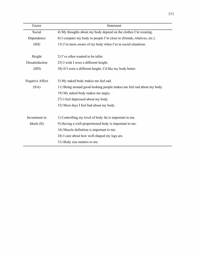
111

Factor Statement

Social

Dependence

(SD)

4) My thoughts about my body depend on the clothes I’m wearing.

8) I compare my body to people I’m close to (friends, relatives, etc.).

15) I’m more aware of my body when I’m in social situations.

Height

Dissatisfaction

(HD)

2) I’ve often wanted to be taller.

25) I wish I were a different height.

38) If I were a different height, I’d like my body better.

Negative Affect

(NA)

5) My naked body makes me feel sad.

11) Being around good-looking people makes me feel sad about my body.

19) My naked body makes me angry.

27) I feel depressed about my body.

33) Most days I feel bad about my body.

Investment in

Ideals (II)

1) Controlling my level of body fat is important to me.

9) Having a well-proportioned body is important to me.

16) Muscle definition is important to me.

24) I care about how well-shaped my legs are.

31) Body size matters to me.

CALIBRATION AND VALIDATION OF THE BODY SELF … · CALIBRATION AND VALIDATION OF THE BODY...

Documents

Transcript of CALIBRATION AND VALIDATION OF THE BODY SELF … · CALIBRATION AND VALIDATION OF THE BODY...