Caldes V8 Developer Introduction · Caldes V8 Developer Introduction Caldes V8 Developer is an all...
30
V8Developer.com Manual V1.22 P.1 Caldes V8 Developer Introduction Caldes V8 Developer is an all new version of the original Caldes Development Valuer Software that has been used to successfully appraise billions of Pounds worth of property development over the past 20 years. The original software, written by the same team, back in 1995, used a standalone Excel engine, but this will no longer work on the latest version of Windows. The all new version works as a cloud based Add-In to Microsoft Excel, as we felt this was the most powerful option available. Easy and reliable The system uses the power of Excel and an enormous amount of work, to provide you with a safe, repeatable and structured tool for appraising the viability of property development schemes. Simply add information to any white cell. Any coloured cell is locked. The only exception to this is drop down lists. Future Proof Because the system is on the cloud, new releases and upgrades are instantly available. Once your Add-In is installed, there is little else you need to do. Just use your files like any other Excel file, saving them to your own computer a network share or the cloud. Here are some of the features: • Add up to 50 units and infinite sub units • Add up to 150 other costs • Add up to 100 additional income row • Cash flow automatically extends out to 10 years • Goal seek land value based on a profit target • Instant sensitivity • Open market and affordable housing comparison table • Full stamp duty calculations Contact information: www.V8Developer.com
Transcript of Caldes V8 Developer Introduction · Caldes V8 Developer Introduction Caldes V8 Developer is an all...
V8Developer.com Manual V1.22 P.1
Caldes V8 Developer Introduction
Caldes V8 Developer is an all new version of the original Caldes Development Valuer Software that has been used to successfully appraise billions of Pounds worth of property development over the past 20 years.
The original software, written by the same team, back in 1995, used a standalone Excel engine, but this will no longer work on the latest version of Windows.
The all new version works as a cloud based Add-In to Microsoft Excel, as we felt this was the most powerful option available.
Easy and reliable
The system uses the power of Excel and an enormous amount of work, to provide you with a safe, repeatable and structured tool for appraising the viability of property development schemes. Simply add information to any white cell. Any coloured cell is locked. The only exception to this is drop down lists.
Future Proof
Because the system is on the cloud, new releases and upgrades are instantly available. Once your Add-In is installed, there is little else you need to do. Just use your files like any other Excel file, saving them to your own computer a network share or the cloud.
Here are some of the features:
• Add up to 50 units and infinite sub units
• Add up to 150 other costs
• Add up to 100 additional income row
• Cash flow automatically extends out to 10 years
• Goal seek land value based on a profit target
• Instant sensitivity
• Open market and affordable housing comparison table
• Full stamp duty calculations
Contact information:
www.V8Developer.com
V8Developer.com Manual V1.22 P.2
Caldes V8 Developer
Appraisal and Viability Toolkit
Sections:
1. System background
2. Getting Started
3. Overview of the Spreadsheets
4. The ‘New Project Wizard’
5. The Task Pane Controls
6. Printing and PDFs
7. Troubleshooting
V8Developer.com Manual V1.22 P.3
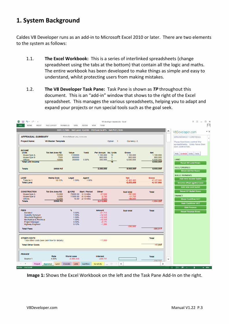
1. System Background
Caldes V8 Developer runs as an add-in to Microsoft Excel 2010 or later. There are two elements to the system as follows:
1.1. The Excel Workbook: This is a series of interlinked spreadsheets (change spreadsheet using the tabs at the bottom) that contain all the logic and maths. The entire workbook has been developed to make things as simple and easy to understand, whilst protecting users from making mistakes.
1.2. The V8 Developer Task Pane: Task Pane is shown as TP throughout this document. This is an “add-in” window that shows to the right of the Excel spreadsheet. This manages the various spreadsheets, helping you to adapt and expand your projects or run special tools such as the goal seek.
Image 1: Shows the Excel Workbook on the left and the Task Pane Add-In on the right.
V8Developer.com Manual V1.22 P.4
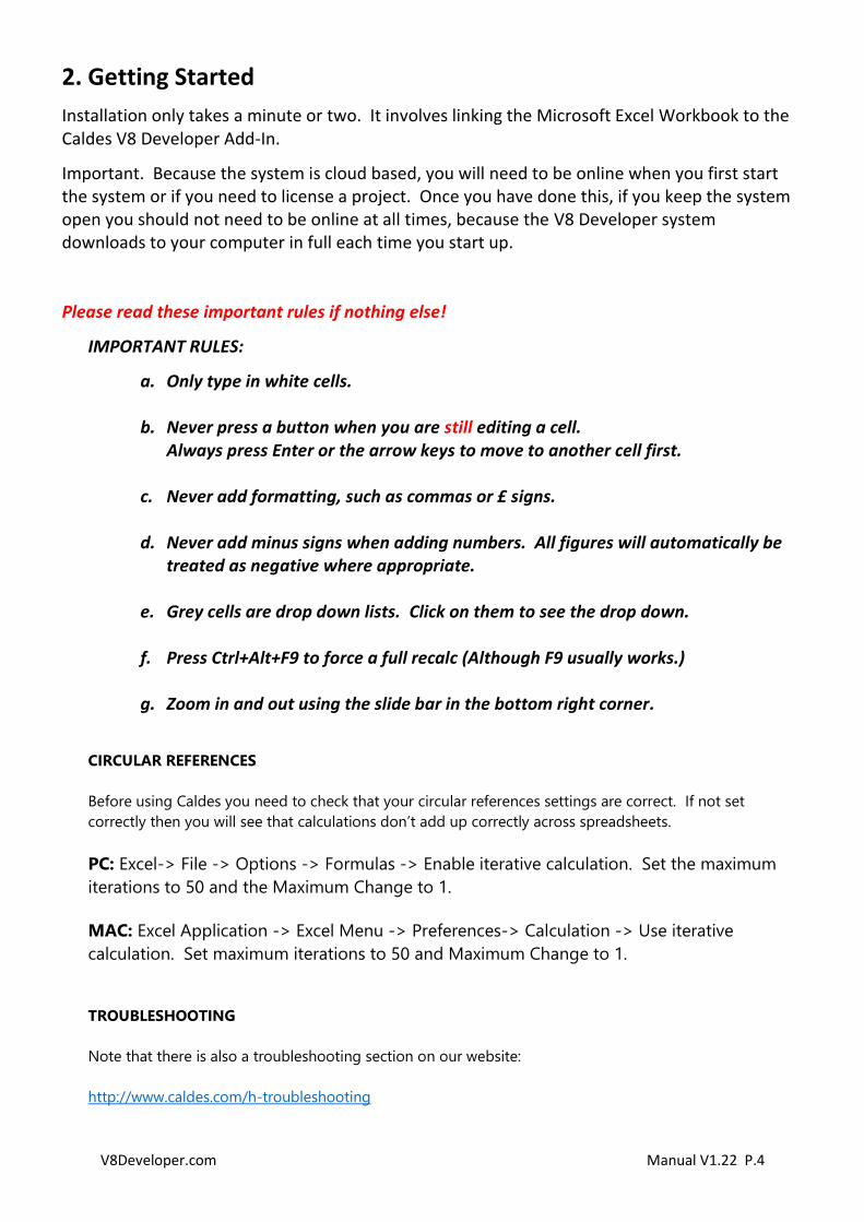
2. Getting Started
Installation only takes a minute or two. It involves linking the Microsoft Excel Workbook to the Caldes V8 Developer Add-In.
Important. Because the system is cloud based, you will need to be online when you first start the system or if you need to license a project. Once you have done this, if you keep the system open you should not need to be online at all times, because the V8 Developer system downloads to your computer in full each time you start up.
Please read these important rules if nothing else!
IMPORTANT RULES:
a. Only type in white cells.
b. Never press a button when you are still editing a cell. Always press Enter or the arrow keys to move to another cell first.
c. Never add formatting, such as commas or £ signs.
d. Never add minus signs when adding numbers. All figures will automatically be treated as negative where appropriate.
e. Grey cells are drop down lists. Click on them to see the drop down.
f. Press Ctrl+Alt+F9 to force a full recalc (Although F9 usually works.)
g. Zoom in and out using the slide bar in the bottom right corner.
CIRCULAR REFERENCES
Before using Caldes you need to check that your circular references settings are correct. If not set
correctly then you will see that calculations don’t add up correctly across spreadsheets.
PC: Excel-> File -> Options -> Formulas -> Enable iterative calculation. Set the maximum
iterations to 50 and the Maximum Change to 1.
MAC: Excel Application -> Excel Menu -> Preferences-> Calculation -> Use iterative
calculation. Set maximum iterations to 50 and Maximum Change to 1.
TROUBLESHOOTING
Note that there is also a troubleshooting section on our website:
http://www.caldes.com/h-troubleshooting
V8Developer.com Manual V1.22 P.5
2.1. Installation in brief: 2.1.1. You will only have to do this once and if you are reading this document
then this may have been done already, but we have added this here in case the information is needed.
2.1.2. Install Excel 2013 or later (Or Excel for Mac / iPad)
2.1.3. Go to the downloads page on www.v8developer.com for detailed installation instructions.
2.1.4. If you want to install the latest template file, you can just run the setup program again.
2.2. Starting a new project: 2.2.1. If already in Excel, close it then open the spreadsheet template. This
will have been installed to your computer in the following location: Documents\V8Developer\excel_template\V8-developer-master.xltx There may also be a short cut on your desktop called V8Developer, with an Excel Icon. This takes you straight to the template.
2.2.2. Open the V8 Developer Add-In: Excel Menu: Insert-> My Apps -> Shared Folder -> V8Developer.com
2.2.3. Add your username and password and follow instructions.
2.2.4. Run the “H1: New project wizard” button. This is ALWAYS the best way to start a new project.
2.2.5. DEFAULT DOCUMENT: Note that you don’t have to log in every time you start a new project. To speed things up, do the following:
• Start a new project but do not change anything.
• License the project via the license button
• Click the restart button.
• Save the project as a new file. When it asks you for the file name etc, change the file type to 'Excel Template (*.xltx)
• Change the folder to Documents/V8Developer/excel_template* and save over the V8-Developer-master.xltx file, replacing the start-up file with your registered one.
• Close Excel. It is important that you completely quit. Then you can start again from the desktop shortcut.
V8Developer.com Manual V1.22 P.6
• You will still have to log in from time to time but you won't have to do the above again until your license expires at the end of your license period or until you upgrade your template file. *This location could be different on your computer. If in doubt, right click on the V8Developer short cut on your desktop and select properties. Then look at the Target box to see the full path.
2.3. Saving a project:
2.3.1. Save your Workbook like you would any other workbook. You can save
it to your hard disk or the cloud (E.g. Microsoft OneDrive)
2.4. Open a project: 2.4.1. Open your saved Workbook and the V8 Developer Task Pane will
automatically open too. If not, find it from: Excel Menu: Insert-> My Apps -> Shared Folder -> V8Developer.com
2.5. Diagnosing an error message: 2.5.1. The spreadsheet is controlled by the Task Panel, but you can also do
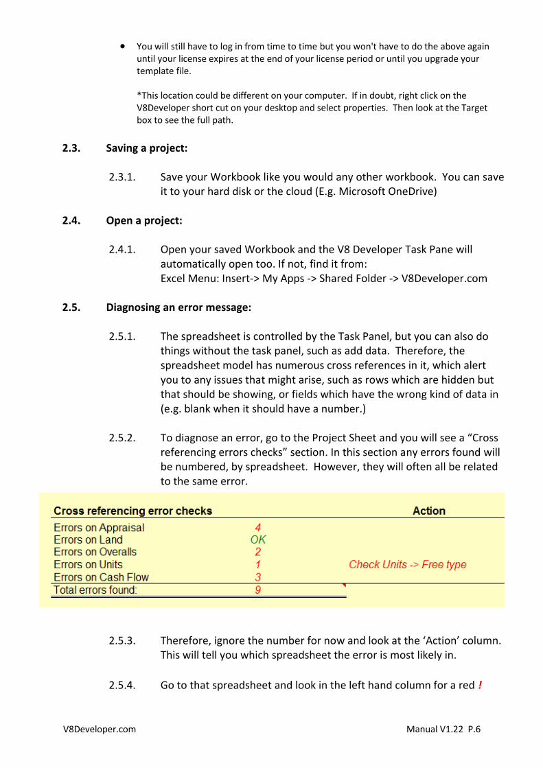
things without the task panel, such as add data. Therefore, the spreadsheet model has numerous cross references in it, which alert you to any issues that might arise, such as rows which are hidden but that should be showing, or fields which have the wrong kind of data in (e.g. blank when it should have a number.)
2.5.2. To diagnose an error, go to the Project Sheet and you will see a “Cross referencing errors checks” section. In this section any errors found will be numbered, by spreadsheet. However, they will often all be related to the same error.
2.5.3. Therefore, ignore the number for now and look at the ‘Action’ column.
This will tell you which spreadsheet the error is most likely in.
2.5.4. Go to that spreadsheet and look in the left hand column for a red !
V8Developer.com Manual V1.22 P.7
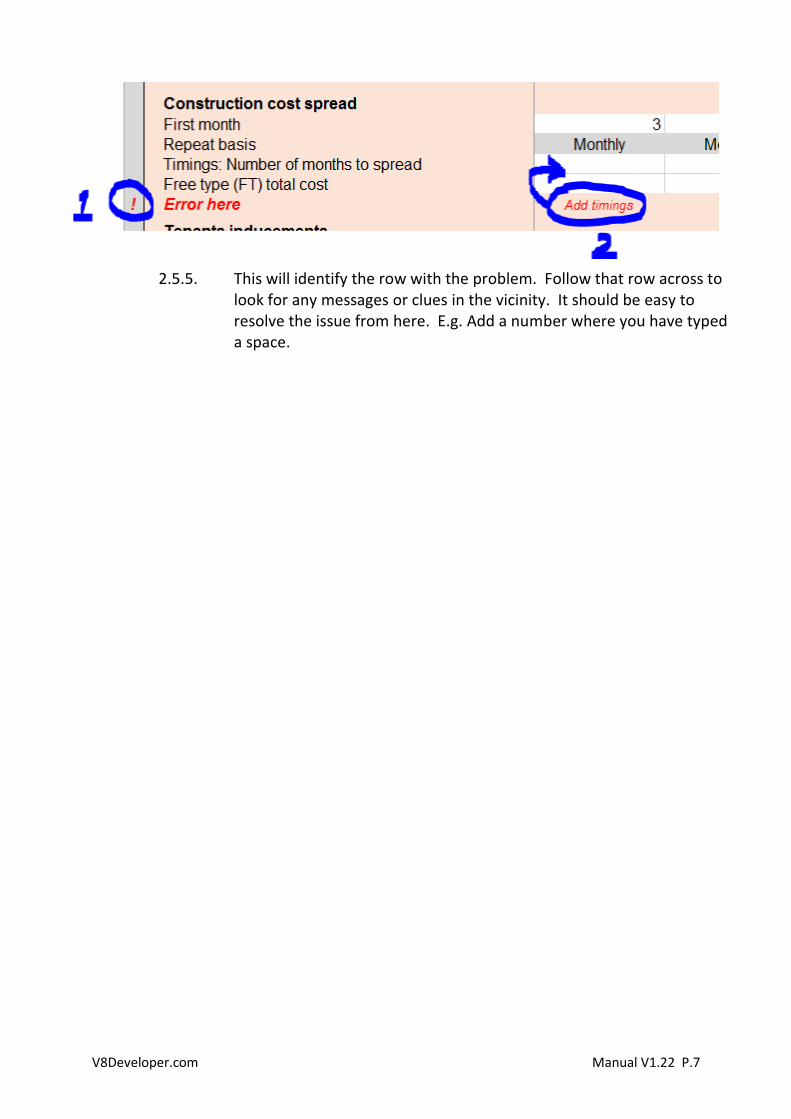
2.5.5. This will identify the row with the problem. Follow that row across to look for any messages or clues in the vicinity. It should be easy to resolve the issue from here. E.g. Add a number where you have typed a space.
V8Developer.com Manual V1.22 P.8
3. Overview of the Spreadsheets
There are 11 spreadsheets in the workbook. Search this PDF for keywords to find out more information on specific items.
The best way to create a new project is to run the ‘New Project Wizard’. This is done via Button H1 in the Task Pane (TP).
IMPORTANT RULES: Only type in white cells.
Never add formatting, such as commas or £ signs.
Never add minus signs when adding numbers. All figures will automatically be treated as negative where appropriate.
Grey cells are drop down lists. Click on them to see the drop down.
3.1. Sheet1 This sheet holds some basic instructions, but once you know these you can delete them and use this sheet for your own purposes, such as a Quantity Surveyors figures. You can feed these figures in to any white cell in Caldes using normal Excel functions.
3.2. Project sheet The project spreadsheet holds the key project information including: 3.2.1. Project name. This is really just a reference and does not need to be
related to the filename, but usually will be.
3.2.2. Option. Add an option reference number here. Usually users just start with 1, or A and then as the project varies they might change this.
3.2.3. Postal town. Add the nearest postal town here. We intend to use a lookup system to get default values based on the town, in the future.
3.2.4. Units. Click on the grey cell and you will see a small drop down button to the right. This is the same for all grey cells. You can then change the units accordingly. Changing from Metric to Imperial, or visa versa, will not affect any calculations or convert any figures. All it does is change the labels.
3.2.5. Currency. Add your currency here, e.g. £ or $. Changing this will not change or convert any figures. All it does is change the labels.
V8Developer.com Manual V1.22 P.9
3.2.6. Project start. Add a project start date. The day will not show but you should always add the first day of the month, even if the project doesn’t actually start on the 1st. E.g. 01/12/2016. If for some reason your dates are shown in USA format, add the date in long format. E.g. 01 December 2016 and the date will correct itself. We recommend that you start on a ‘quarter month’, e.g. Jan, April, July or October.
3.2.7. Goal Seek: Total Net Land Value. If you know the total land value of all tranches of land, add this here or add a guess as a starting point. The Land sheet will hold a breakdown of the various land payments, but this is where you add the total cost. If you don’t know what the land will cost, add a ‘Profit on GDC target’ (see below for more details)
3.2.8. Goal Seek: Profit on Cost target (default). If you know the profit that you want, e.g. 20%, add this here. Then go to TP-> Tools -> T2: Goal Seek Profit on GDC. This will then calculate the land value for you, to meet that profit. You have to run this tool every time you want to find the new land value. The appraisal (land section) and project (goal seek section) sheets will warn you if you are off target by showing a warning message in red next to these cells. If you don’t want to see the warning, add a value of 0 to this cell and it will be ignored. When starting a new project, we recommend that you leave this at 0 until you have added all of your other figures.
3.2.9. Goal Seek: Profit on GDV target. This is as above, but for the profit on Gross Development Costs, as is regularly used in residential developments. To change from Profit on Cost (default) to GDV, click on the grey ‘Profit on Cost’ cell. This will then provide you with a drop down list icon at the end of the cell. Change to Profit on GDV by clicking on the drop down list icon.
3.2.10. Cross referencing error checks. Check this section periodically to see if
there are any errors in your spreadsheets and what to do about them. The V8 Developer tool will also check for errors and the core spreadsheets will show a warning too in the top left hand corner. Usually a quick recalculation of the relevant spreadsheet will be required. To recalculate a sheet, go to Excel -> Formulas -> Calculate Sheet. If this does not fix the errors, check for any on screen instructions and if necessary, click the ‘H4: System Health Check’ button.
3.2.11. Profit Split. You can use this to work out how the profits will be split. These figures are deliberately left out of the appraisal and do not affect the actual project figures and you can ignore this section if it is of no interest to you. These figures are just a split of the profit. The
V8Developer.com Manual V1.22 P.10
priority coupon is a figure that is paid out first, usually to the party that is putting in the most money. They will get this money before any more profits are shared. Add 0% to ignore this section. Then the rest of the profit might be split up between 2 or more parties. You can add a percentage or amount to any of the boxes. Just remember that if there is not enough money to cover all of the splits then payments will be made in order of priority from the top cell down.
3.2.12. License. Each Workbook needs to be license before you can use it. The V8 Developer system should guide you through this, asking you for your email address and then password. You can do this at any time by clicking the ‘H2: Log in’ button. Once a workbook is licensed, the system will periodically re-check the license in the background. Follow any instructions given in this area to license a project.
3.2.13. Template version. The current template version will show at the bottom of the Project sheet. This is used by the software to check which features are compatible. If a newer template is available then the system will alert you to this, but only update if you are starting a new project. All existing projects will remain compatible with the V8 Developer system.
3.3. Appraisal sheet This is a summary of the entire project and pulls together all the information from the other sheets. Each section is colour coded. As you use the system you will get used to the colours and find it easier to navigate. Here are a few specifics: 3.3.1. Grey summary bar. Along the top of each sheet is a summary bar.
This holds key information, which will change dynamically as you change the figures.
3.3.2. Button column. On the right hand side is a column which has the word ‘Button’ at the top. In the column, there is a light grey box for each section. If you see an exclamation sign in the box, then this is a warning that there is nothing in that row. That might be correct (it won’t print) but if not, click the relevant TP button. E.g. If you see a ! in the land section, then L1 means click button L1 in the green ‘Controls’ section of the TP. The row will then be hidden if it is not in use (but it might stay open if the section is in use, but has zero value, such as a unit costs but no income.)
V8Developer.com Manual V1.22 P.11
3.3.3. Appraisal Task Pane (TP) control buttons. L1: Reset All Land Rows: There are no buttons in the TP relevant to the Appraisal spreadsheet specifically.
3.3.4. IRR. The Internal Rate of Return (IRR) is calculated on the net monthly cash flow inc VAT (cash flow row 987), before any finance and then shown on the appraisal (row 255) and cash flow (row 991)
3.4. Land sheet 3.4.1. Gross site area. Add the number of acres or hectares here and the net
number of developable acres or hectares. You will then see a cost per acre.
3.4.2. Total Net Land Cost. This is the same figure as set in the Project Sheet. To change it, go to the project sheet.
3.4.3. Tranches Tranche 1 is the main tranche of land. If you add additional tranches (2,3 or 4) then these will always come off Tranche 1. In other words, you are simply splitting up the entire land cost into smaller amounts, not adding additional land costs.
3.4.4. Stamp duty: Click the grey ‘Residential’ or ‘Commercial’ drop down box to change the stamp duty calculation. Leave the stamp duty land tax box blank for an automatic calculation. Or type in the value or percentage if preferred. You can also set whether stamp duty is paid on top of VAT. For overseas countries where there is no stamp duty, add 0.00% to the stamp duty box.
3.4.5. Land Task Pane (TP) control buttons. L1: Reset All Land Rows: If you have added or removed a tranche of land, click this button and V8 Developer will check all sheets to make sure that the correct rows and columns are showing or hidden.
3.5. Overalls sheet
3.5.1. Project construction fees. Add in the name followed by a percentage or amount here. You can add up to 20 fees. If a percentage then it will automatically calculate as a percentage of the Total Construction. Fees are paid pro-rata the spread of construction costs. This gives a
V8Developer.com Manual V1.22 P.12
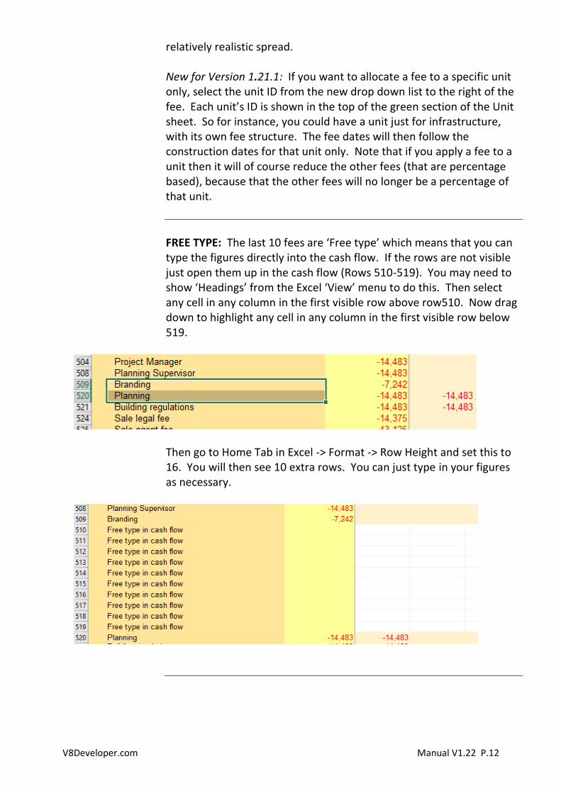
relatively realistic spread. New for Version 1.21.1: If you want to allocate a fee to a specific unit only, select the unit ID from the new drop down list to the right of the fee. Each unit’s ID is shown in the top of the green section of the Unit sheet. So for instance, you could have a unit just for infrastructure, with its own fee structure. The fee dates will then follow the construction dates for that unit only. Note that if you apply a fee to a unit then it will of course reduce the other fees (that are percentage based), because that the other fees will no longer be a percentage of that unit.
FREE TYPE: The last 10 fees are ‘Free type’ which means that you can type the figures directly into the cash flow. If the rows are not visible just open them up in the cash flow (Rows 510-519). You may need to show ‘Headings’ from the Excel ‘View’ menu to do this. Then select any cell in any column in the first visible row above row510. Now drag down to highlight any cell in any column in the first visible row below 519.
Then go to Home Tab in Excel -> Format -> Row Height and set this to 16. You will then see 10 extra rows. You can just type in your figures as necessary.
V8Developer.com Manual V1.22 P.13
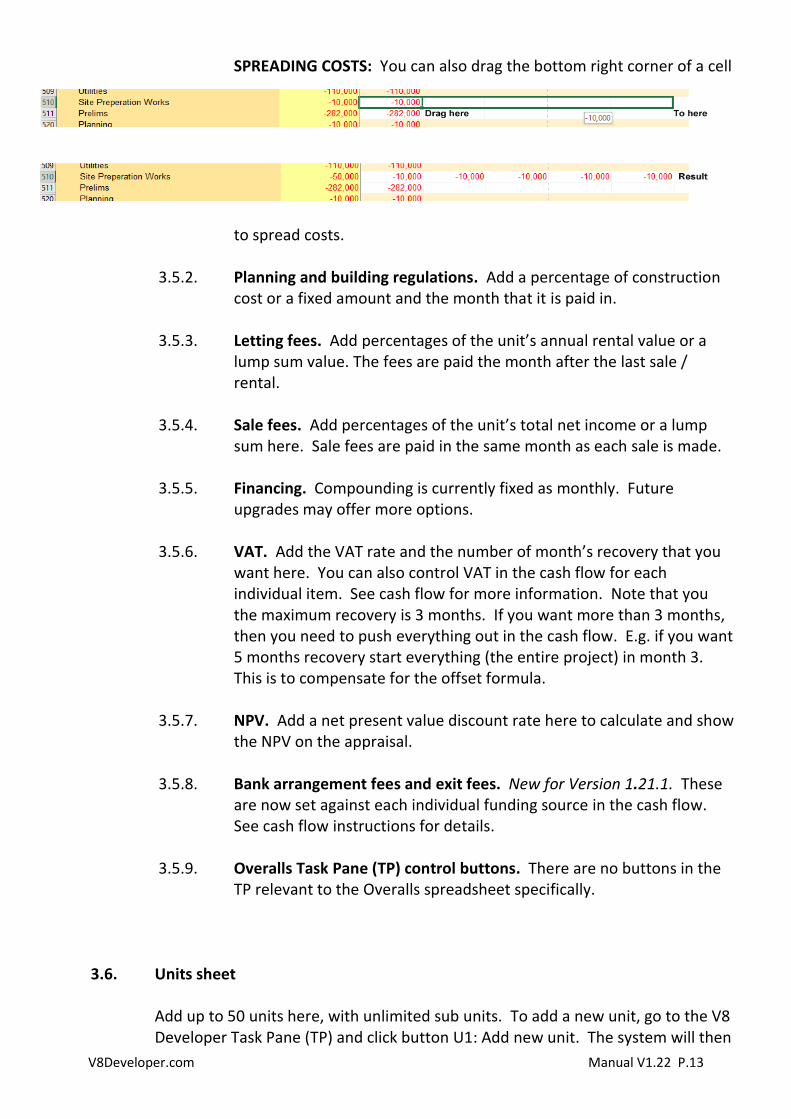
SPREADING COSTS: You can also drag the bottom right corner of a cell
to spread costs.
3.5.2. Planning and building regulations. Add a percentage of construction cost or a fixed amount and the month that it is paid in.
3.5.3. Letting fees. Add percentages of the unit’s annual rental value or a lump sum value. The fees are paid the month after the last sale / rental.
3.5.4. Sale fees. Add percentages of the unit’s total net income or a lump sum here. Sale fees are paid in the same month as each sale is made.
3.5.5. Financing. Compounding is currently fixed as monthly. Future upgrades may offer more options.
3.5.6. VAT. Add the VAT rate and the number of month’s recovery that you want here. You can also control VAT in the cash flow for each individual item. See cash flow for more information. Note that you the maximum recovery is 3 months. If you want more than 3 months, then you need to push everything out in the cash flow. E.g. if you want 5 months recovery start everything (the entire project) in month 3. This is to compensate for the offset formula.
3.5.7. NPV. Add a net present value discount rate here to calculate and show the NPV on the appraisal.
3.5.8. Bank arrangement fees and exit fees. New for Version 1.21.1. These are now set against each individual funding source in the cash flow. See cash flow instructions for details.
3.5.9. Overalls Task Pane (TP) control buttons. There are no buttons in the TP relevant to the Overalls spreadsheet specifically.
3.6. Units sheet Add up to 50 units here, with unlimited sub units. To add a new unit, go to the V8 Developer Task Pane (TP) and click button U1: Add new unit. The system will then
V8Developer.com Manual V1.22 P.14
add a new blank unit for you. Simply fill out the 3.6.1. Adding a new unit. Add up to 50 units here, with unlimited sub units.
To add a new unit, go to the V8 Developer Task Pane (TP) and click button ‘U1: Add New Unit’. The system will then add a new blank unit for you. Simply fill out the white cells in the blank column. Each unit is separated out with a green section for income and a pink section for costs.
3.6.2. Unit name. Simply add the name of the unit here, e.g. Unit 1, Type A etc. This WILL show in the appraisal and cash flow. You can also type in the cell above. Eg Type A or Group A etc. This will not show in the appraisal and cash flow. It is simply a note cell.
3.6.3. Sort order. Add the sort order as a number here. You can use this later to sort units. See U5: Sort wizard for details.
3.6.4. Description. Use this to add a short description for your own purposes. This will NOT show in the appraisal or cash flow.
3.6.5. Unit ID. Regardless of name or sort order, the ID is the unique number of that unit.
3.6.6. Quantity / Sub Units. Most of the time you will just add 1 here. But if you have multiple identical units, then add how many here and everything will be multiplied by that number for this column.
3.6.7. Internal Area per sub unit. Add the internal / net / rentable area of each sub unit here. The external / gross area is added later. This area will be used to calculate the value, unless you add a lump sum value in the next box.
3.6.8. Rent / area or unit value Option 1: Add a commercial rental value. E.g. if the rental value is £25 per square foot, add 25 here. This figure will then be multiplied by the Internal Area to create an Annual Rental Value (ARV). The ARV is then multiplied by the yield to create a total Net Income for the unit. Option 2: Add a residential rental value. E.g. if the rent per square foot is £200 then add 200 here. This is multiplied by the Internal floor area to give you a total unit income. Leave the yield blank. Option 3: Add a sale value. E.g. if the sale value of the property is £250,000, add 250000 here. Leave the yield blank.
V8Developer.com Manual V1.22 P.15
Also see Threshold Rent and ARV method in in the Calculations section below.
3.6.9. Ground rent. If there is a ground rent, add it here as a lump sum figure or as a percentage of the Annual Rental Value (ARV).
3.6.10. Yield. This will typically only be used on commercial properties. See Rent / area or unit value above.
3.6.11. Stamp duty. Select the stamp duty calculation from the drop down, by clicking on the grey cell then clicking on the drop down list option to the right of the cell. The stamp duty will automatically be calculated so long as the Purchasers acquisition cost cell is blank below. Alternatively add your own figure to the Purchasers acquisition costs cell.
3.6.12. Purchaser’s acquisition costs. If you leave this cell blank, then a figure will automatically be calculated based on the stamp duty (see stamp duty above). If you want nothing at all, add a zero, not blank. Alternatively, you can add a lump sum or a percentage. If a percentage then see ‘Purchasers cost methods’ below to see how this is calculated.
3.6.13. Purchaser’s finance costs. Add a lump sum amount or percentage. If a percentage then see ‘Purchasers cost methods’ below to see how this is calculated.
3.6.14. To Let Fees: If you want letting agent and legal fees added to this unit add a ‘Y’ to this box. If not, add anything else or leave it blank.
3.6.15. CALCULATIONS:
3.6.16. Threshold rent. V8 Developer uses this value to decide if the figure in the “Rent / area or unit value” box is a rental value or a sale value. This allows you to work in different currencies or high value areas.
3.6.17. ARV method. Method 1 uses the total of all income values that are less than the threshold value (i.e. excludes lump sum values.) Method 2 uses the sum of all income values where 'To Let' Fees = "Y" including lump sum values. Method 2 is the default setting.
V8Developer.com Manual V1.22 P.16
3.6.18. Sensitivity calculations: You can instantly change the value of all units using the mini sensitivity and see the effect. For more information, see the Sensitivity section.
3.6.19. Purchasers cost methods. There are two ways of calculating the purchaser’s acquisition cost and finance costs as follows: Purchasers cost method 1: A percentage including the cost itself: This will be a percentage of the ‘Total Net Unit Income’ after taking off the purchasers’ costs (i.e. after taking itself off.) This is the more commonly used method and gives you a slightly better unit value. Purchasers cost method 2: A percentage excluding the cost itself. This will be a percentage of the ‘Value at yield / Gross Capital Value’ (i.e. it does not include itself within the percentage.) This method is less commonly used and gives you a slightly worse unit value. Note that if you auto calculate the stamp duty then this cost is just removed from the ‘Value at yield / Gross Capital Value’ as per method 2.
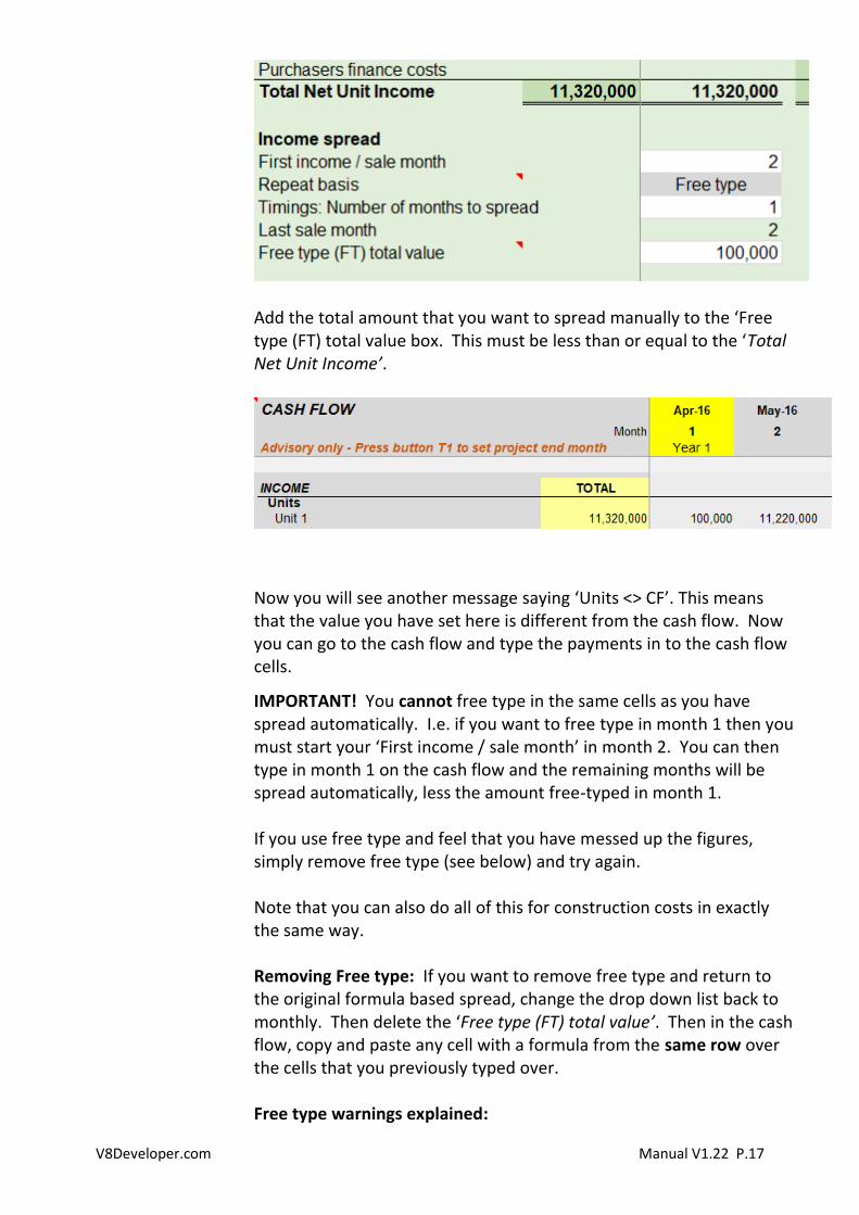
3.6.20. Income spread. First income month: Add the month that the first lump of income for this unit will be paid. If you only have one payment for this unit then leave everything else as default. Spread payments: If you want to spread the payments automatically over a number of months, add in the number of months that you want to spread the payments over to the ‘Number of months to spread’ box. Free type income: Free type provides you with complete flexibility to type in the payments as they happen, rather than the automated spread. This is something that you often want to do as the project matures and you find that you know the more detailed figures. If you want to create a detailed bespoke income plan, click on the ‘Monthly’ grey cell and change this to ‘Free type’ using the drop down list to the right of the grey cell. You will see the words ‘Add above’ in red. This is to highlight which units are set as free type but do not have a value in the cash flow. In the example we are free typing 100,000 out of a total of 11,320,000.
V8Developer.com Manual V1.22 P.17
Add the total amount that you want to spread manually to the ‘Free type (FT) total value box. This must be less than or equal to the ‘Total Net Unit Income’.
Now you will see another message saying ‘Units <> CF’. This means that the value you have set here is different from the cash flow. Now you can go to the cash flow and type the payments in to the cash flow cells.
IMPORTANT! You cannot free type in the same cells as you have spread automatically. I.e. if you want to free type in month 1 then you must start your ‘First income / sale month’ in month 2. You can then type in month 1 on the cash flow and the remaining months will be spread automatically, less the amount free-typed in month 1. If you use free type and feel that you have messed up the figures, simply remove free type (see below) and try again. Note that you can also do all of this for construction costs in exactly the same way. Removing Free type: If you want to remove free type and return to the original formula based spread, change the drop down list back to monthly. Then delete the ‘Free type (FT) total value’. Then in the cash flow, copy and paste any cell with a formula from the same row over the cells that you previously typed over. Free type warnings explained:
V8Developer.com Manual V1.22 P.18
Del FT val: This means you do not have the repeat basis set to Free type, yet you have a free type value. So you need to delete that value or change the repeat basis to Free type.
Add above: You have set the repeat basis to Free type but you have not set a total free type value. Add a value to the Free type total box. This must be the sum of all the individual amounts in the cash flow that you do not want automatically calculated. Units <> CF: This means that you have Free type set and you have added a total value to the Units sheet, but this does not match the sum of all the payments for that unit in the Cashflow (you might not have added any to the white cells in the cash flow yet, which is fine.) To resolve this, change the cash flow or the unit total amount as necessary. To help with this, the discrepancy is shown in the Cashflow after the unit name in brackets. E.g. Unit 1 (FT:3000) means that the free type total is short by £3,000 for Unit 1. Unit costs As with the income section, simply fill out the white cells in the cost section. At the top of the cost section is a reminder of the number of sub units and the Internal / Net area.
3.6.21. Construction area per sub unit. Add in the gross / external construction floor area here. This will naturally be slightly larger than the internal / net area.
3.6.22. Cost per area / Unit cost. Type in a cost per area, e.g. for £50 per square foot type in 50. Or if you know the exact lump sum cost you can type that in here instead. E.g. 100000 for £100,0000. If you have multiple sub units then the figure here is per sub unit and then multiplied later (in the same way that the income section is calculated.)
3.6.23. Contingency. Most construction projects will add in a little contingency of say 5% - 10%.
3.6.24. Other lump sums. If you have any other fixed costs, type them in here. You can rename the rows if you like, by typing in the white cells. These lump sums will all be spread over the construction period in the same ratio as the rest of the construction costs above. The options for how construction costs are spread are set out in the ‘Construction cost spread’ section.
3.6.25. Calculations:
V8Developer.com Manual V1.22 P.19
3.6.26. Threshold cost. This is the value at which the figure in the ‘Cost per sq ft / Unit cost’ box changes from a rate to a lump sum. This allows you to work in different currencies or high cost areas.
3.6.27. Construction area sensitivity. You can instantly change all the construction areas using the mini sensitivity analysis. See the Sensitivity sheet for more information. The same goes for the Cost per area.
3.6.28. Construction cost spread: First month: Add the first month that you want construction costs for each unit. Repeat basis: Then select the repeat basis, by clicking on the grey cell and then selecting the options from the drop down list. Monthly will spread the costs evenly. S-Curve will spread the costs on a typical S-Curve, with low costs at the beginning, peaking in the middle and dropping off at the end. This is the default value. Free type allows you to type the spread of costs directly in to the cash flow (Just like you can on income. See the income section for details on how this works. They both work the same way.) Number of months to spread: If you want all the costs in one month, just add 1 to the number of months to spread. Alternatively add a number of months here and the construction costs will be split evenly over X months, starting from the ‘First month’.
3.6.29. Tenants inducements. If you add tenants’ inducements this opens up a whole new section in the appraisal and cash flow. Lump sum: Add any fixed lump sum amount here. Rent free period in months: Add the number of months’ rent free period that you will be offering here. This is typically as an alternative to the lump sum amount. Rent free period cost: This will be automatically calculated from the rent
V8Developer.com Manual V1.22 P.20
Month paid: Add in the month that you want this paid, or leave it blank and it will automatically be paid at the end of construction.
3.6.30. Sub type breakdown. This is simply a table showing how your project is broken down, by different unit subtypes.
3.6.31. Units Task Pane (TP) control buttons:
3.6.32. U1: Add new unit. Click this button to add a new unit. This will be added to the end / bottom of the current list of units and will then show in the Appraisal, Units sheet and Cashflow sheet. Follow on screen instructions.
3.6.33. U2: Remove unit wizard. If you want to remove a unit, click this button and follow on screen instructions.
3.6.34. U3: Reset rows and columns. If you have added a few units, removed some units or changed values etc then you could be left with some blank units showing. Click this button to reset all the rows and columns throughout the system. This function is also covered in the Health-check.
3.6.35. U4: Reset Cashflow formula. If you have typed over the income or construction figures in the cash flow with your own spread of payments, using the ‘Free type’ function then you might want to reset the figures back to the default automatic formula. If so, make sure that you have set all units that you want to fix to something other than ‘Free type’ in the Units sheet, then press this button and the system will automatically find and replace all formula. See the ‘Free type’ section above for more information.
3.6.36. U5: Sort Wizard. This allows you to resort your units from the order that they were added. Press the Sort Wizard button to sort your units and follow on screen instructions.
Note: When numbering your units, you can miss out values, for instance if you have groups of units. Eg. You could have three groups of two units with the following sort order values: 1, 2, 10, 11, 20, 21.
V8Developer.com Manual V1.22 P.21
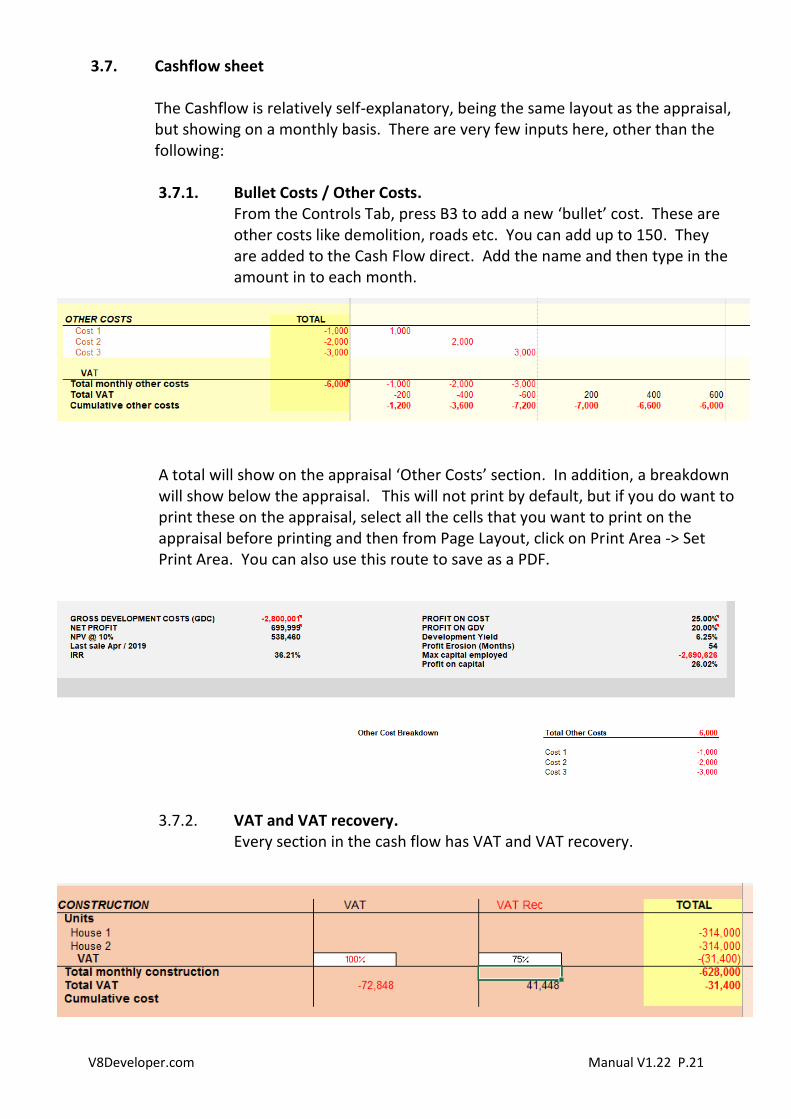
3.7. Cashflow sheet The Cashflow is relatively self-explanatory, being the same layout as the appraisal, but showing on a monthly basis. There are very few inputs here, other than the following: 3.7.1. Bullet Costs / Other Costs.
From the Controls Tab, press B3 to add a new ‘bullet’ cost. These are other costs like demolition, roads etc. You can add up to 150. They are added to the Cash Flow direct. Add the name and then type in the amount in to each month.
A total will show on the appraisal ‘Other Costs’ section. In addition, a breakdown will show below the appraisal. This will not print by default, but if you do want to print these on the appraisal, select all the cells that you want to print on the appraisal before printing and then from Page Layout, click on Print Area -> Set Print Area. You can also use this route to save as a PDF.
3.7.2. VAT and VAT recovery. Every section in the cash flow has VAT and VAT recovery.
V8Developer.com Manual V1.22 P.22
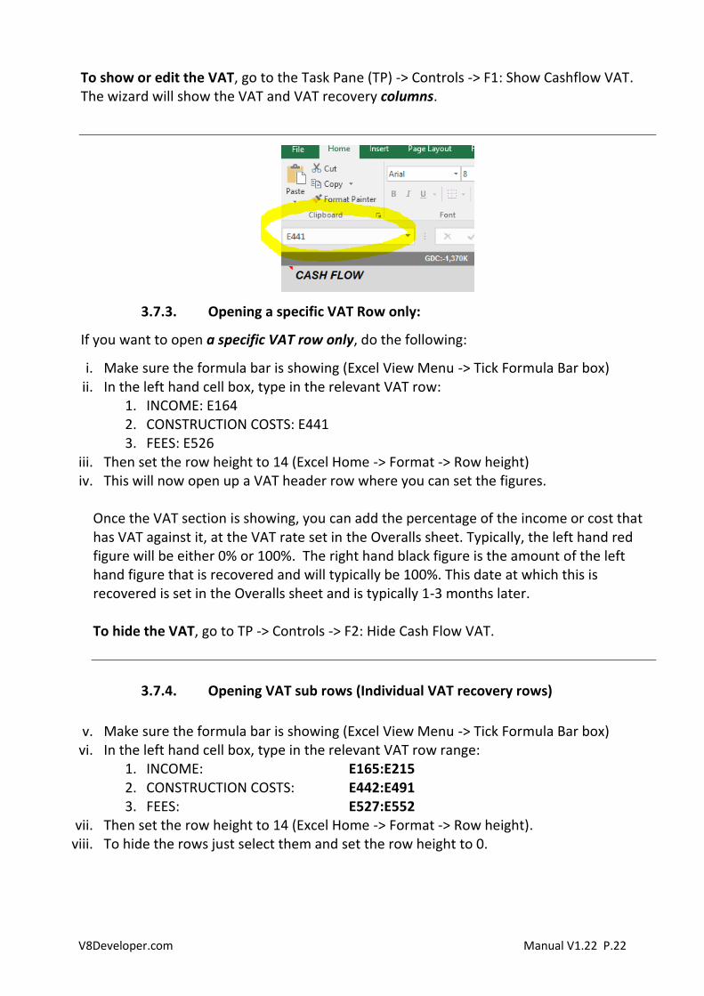
To show or edit the VAT, go to the Task Pane (TP) -> Controls -> F1: Show Cashflow VAT. The wizard will show the VAT and VAT recovery columns.
3.7.3. Opening a specific VAT Row only:
If you want to open a specific VAT row only, do the following:
i. Make sure the formula bar is showing (Excel View Menu -> Tick Formula Bar box) ii. In the left hand cell box, type in the relevant VAT row:
1. INCOME: E164 2. CONSTRUCTION COSTS: E441 3. FEES: E526
iii. Then set the row height to 14 (Excel Home -> Format -> Row height) iv. This will now open up a VAT header row where you can set the figures.
Once the VAT section is showing, you can add the percentage of the income or cost that has VAT against it, at the VAT rate set in the Overalls sheet. Typically, the left hand red figure will be either 0% or 100%. The right hand black figure is the amount of the left hand figure that is recovered and will typically be 100%. This date at which this is recovered is set in the Overalls sheet and is typically 1-3 months later. To hide the VAT, go to TP -> Controls -> F2: Hide Cash Flow VAT.
3.7.4. Opening VAT sub rows (Individual VAT recovery rows)
v. Make sure the formula bar is showing (Excel View Menu -> Tick Formula Bar box) vi. In the left hand cell box, type in the relevant VAT row range:
1. INCOME: E165:E215 2. CONSTRUCTION COSTS: E442:E491 3. FEES: E527:E552
vii. Then set the row height to 14 (Excel Home -> Format -> Row height). viii. To hide the rows just select them and set the row height to 0.
V8Developer.com Manual V1.22 P.23
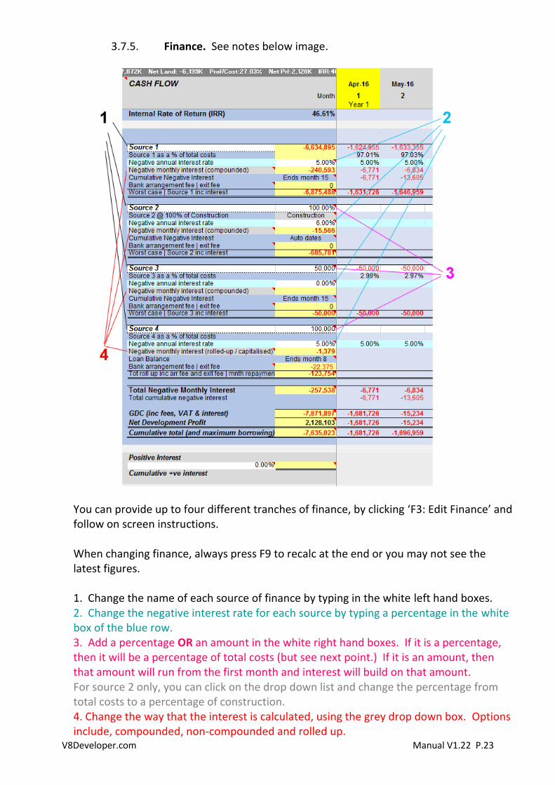
3.7.5. Finance. See notes below image.
You can provide up to four different tranches of finance, by clicking ‘F3: Edit Finance’ and follow on screen instructions. When changing finance, always press F9 to recalc at the end or you may not see the latest figures. 1. Change the name of each source of finance by typing in the white left hand boxes. 2. Change the negative interest rate for each source by typing a percentage in the white box of the blue row. 3. Add a percentage OR an amount in the white right hand boxes. If it is a percentage, then it will be a percentage of total costs (but see next point.) If it is an amount, then that amount will run from the first month and interest will build on that amount. For source 2 only, you can click on the drop down list and change the percentage from total costs to a percentage of construction. 4. Change the way that the interest is calculated, using the grey drop down box. Options include, compounded, non-compounded and rolled up.
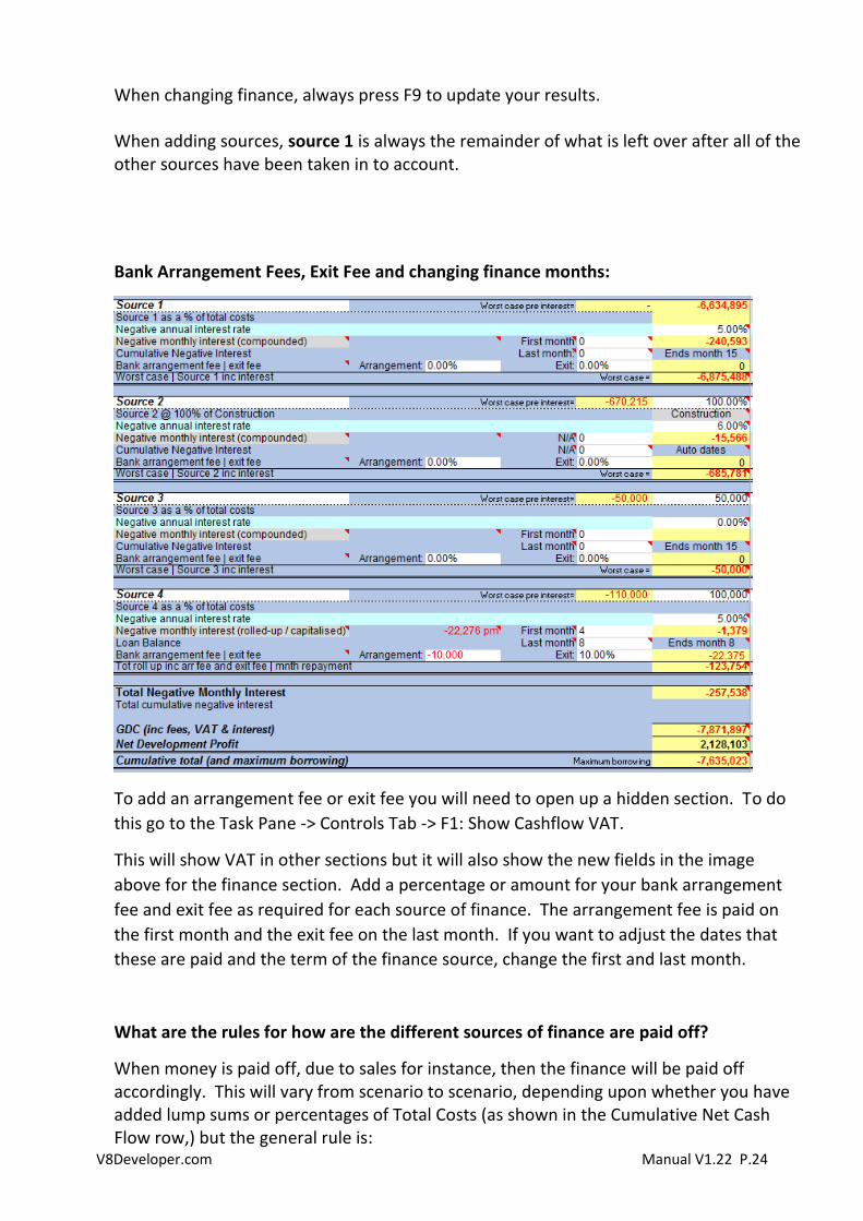
V8Developer.com Manual V1.22 P.24
When changing finance, always press F9 to update your results. When adding sources, source 1 is always the remainder of what is left over after all of the other sources have been taken in to account.
Bank Arrangement Fees, Exit Fee and changing finance months:
To add an arrangement fee or exit fee you will need to open up a hidden section. To do
this go to the Task Pane -> Controls Tab -> F1: Show Cashflow VAT.
This will show VAT in other sections but it will also show the new fields in the image
above for the finance section. Add a percentage or amount for your bank arrangement
fee and exit fee as required for each source of finance. The arrangement fee is paid on
the first month and the exit fee on the last month. If you want to adjust the dates that
these are paid and the term of the finance source, change the first and last month.
What are the rules for how are the different sources of finance are paid off?
When money is paid off, due to sales for instance, then the finance will be paid off accordingly. This will vary from scenario to scenario, depending upon whether you have added lump sums or percentages of Total Costs (as shown in the Cumulative Net Cash Flow row,) but the general rule is:
V8Developer.com Manual V1.22 P.25
If they are all percentages then they will all be paid off at the same time, as and when the project goes positive in the cash flow. If you have added lump sums of borrowing then source 4 will be paid off first, then source 3, 2, 1. If you have a mix of percentages and lump sum borrowing, then each lump sum will be paid off as that lump sum can no longer be supported by the negative cash flow line (Cumulative Net Cash Flow / Total Costs row). I.e. you have made sales bigger that the size of that lump sum borrowing in that source and so that source needs to be paid back. The date that finance is paid off has nothing to do with the negative interest rate that you are paying. I.e. just because you are paying more doesn’t mean it will be paid off quicker, unless you override this (see below). Therefore, the most efficient schemes will have the highest negative interest rate in the source that is paid off the quickest, or borrowed the latest. E.g. you are using your own equity in source 1 and you are borrowing 3 x £1,000,000 (from 3 different sources) at negative interest rates of 4%, 6% and 12% each. In this scenario you would put the 12% in source 4, 6% in source 3, 4% in source 2 and your equity at 0% in source 1. Then the 12% borrowing (source 4) would automatically be drawn down last and paid back first. Source 3 would be drawn down second and paid back third to last. Source 2 would be drawn down third and paid back second to last. Source 1 would be first in and last out. In the real world you might start paying interest on a loan the minute you drawn on that loan. Caldes shows you the importance of not drawing on a loan too early, as this can affect your profit substantially.
Source 2 has a drop down option that allows you to change the finance from Total Costs to a percentage of construction. This is marked with 4 in the image above.
How do I change the negative interest rate on a month by month basis? This applies to template 1.19.1 or later only. You can change the interest rate on a month by month basis on all sources, by typing over the rate in the pale blue row for the relevant source. When you change the rate, that rate will continue for all subsequent months automatically. The code “1” will show in purple above the finance source for the month where you have changed the rate, (unless the rate goes to zero.)
If you have typed over a rate and want to replace the formula, just copy and paste any of the other cells with formulas that are in the same row.
How do I change the finance amount on a month by month basis? This applies to template 1.19.1 or later only. You can change the finance amount on a month by month basis on all sources except source 1, by typing over the amount in the white cells (the same row as the Source name). The code “2” will show in purple above the source where
V8Developer.com Manual V1.22 P.26
this has been done, so that it can be quickly identified. Note that you must add a negative whole number (e.g. -50000) in this row (normally you do not need to add a minus sign.) This will ONLY change in the month where you have overtyped it. All subsequent months will behave as before unless you overtype them too.
If you have typed over an amount and want to replace the formula, just copy and paste any of the other cells with formulas that are in the same row.
3.7.6. Positive Interest. At the bottom of the Cashflow you can add a positive interest rate. This is then reflected in the Appraisal on its own row. Positive interest is only received when the Cashflow ‘Cumulative total’ row is positive, and continues until the last income or cost.
V8Developer.com Manual V1.22 P.27
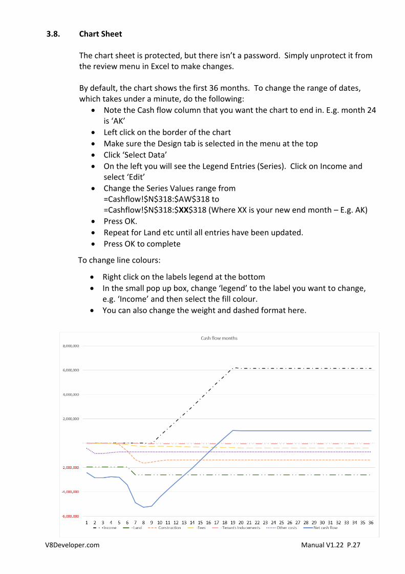
3.8. Chart Sheet The chart sheet is protected, but there isn’t a password. Simply unprotect it from the review menu in Excel to make changes. By default, the chart shows the first 36 months. To change the range of dates, which takes under a minute, do the following:
• Note the Cash flow column that you want the chart to end in. E.g. month 24 is ‘AK’
• Left click on the border of the chart
• Make sure the Design tab is selected in the menu at the top
• Click ‘Select Data’
• On the left you will see the Legend Entries (Series). Click on Income and select ‘Edit’
• Change the Series Values range from =Cashflow!$N$318:$AW$318 to =Cashflow!$N$318:$XX$318 (Where XX is your new end month – E.g. AK)
• Press OK.
• Repeat for Land etc until all entries have been updated.
• Press OK to complete
To change line colours:
• Right click on the labels legend at the bottom
• In the small pop up box, change ‘legend’ to the label you want to change, e.g. ‘Income’ and then select the fill colour.
• You can also change the weight and dashed format here.
V8Developer.com Manual V1.22 P.28
3.9. Sensitivity sheet
This sheet holds a mini sensitivity control. To see the effect of increasing or decreasing the core figures globally, add a positive or negative % figure here. E.g. to increase all rental values by 5%, add 5% to the Rental Value box and you will see the rental value increase by 5%. In addition, the entire Workbook will adjust, so wherever you go this change will be reflected. The Project sheet will show a red Yes in the Cross referencing error checks section, as a warning that you are not looking at the original values.
3.10. Full sensitivity analysis. Add the values that you want to analyse to the white cells in the right hand grey box. Typically these will be 1%-2% variations over 5-10 steps for each axis. The grey cells are drop down boxes. Click on them to change the horizontal axis, the vertical axis and the target result. Remove any figures that you do not want to use from the Mini Sensitivity too (although you can keep figures in here too if you want, but note that they will become overwritten if you are using them in the full sensitivity Axis boxes.) Now go to TP -> Tools -> T3: Sensitivity Analysis and click the button. The table will automatically grow in front of your eyes. If you are looking for the land value at a fixed profit (as set in the Project sheet) then the calculations will take a little longer. Please be patient. You can stop the sensitivity at any time, by simply clicking the button again. Give it a few seconds to come to an end.
3.11. Controls sheet This sheet holds all of the system controls, such as drop down lists, defaults etc. You can ignore this sheet, but do not hide it as this will stop the system from working.
3.12. Revisions sheet This sheet simply lets you know what changes have been made to the template and / or system recently.
3.13. Sheet1 sheet Use this sheet if you want to build in your own tables or analysis on the data, add charts etc. The sheet is unlocked and unrestricted. You can delete all of the information that we have added to this sheet.
V8Developer.com Manual V1.22 P.29
4. The New Project Wizard The new project Wizard is a great place to start if you are new to the program. Click button H1 and follow on screen instructions. One finished, make sure you press H4: System health check, which will double check that everything is OK. You should need to run the health check very often, once a project is set up.
5. The Task Pane Controls. The various controls in the task pane are covered above where applicable and should be very self-explanatory. Select the tab at the top of the task pane to change which buttons show. Have a look at the tabs, which are often updated with new upgrades and cover general help, land, fees, overalls, bullet payments, finance, units and tools (goal seek, sensitivity analysis etc.)
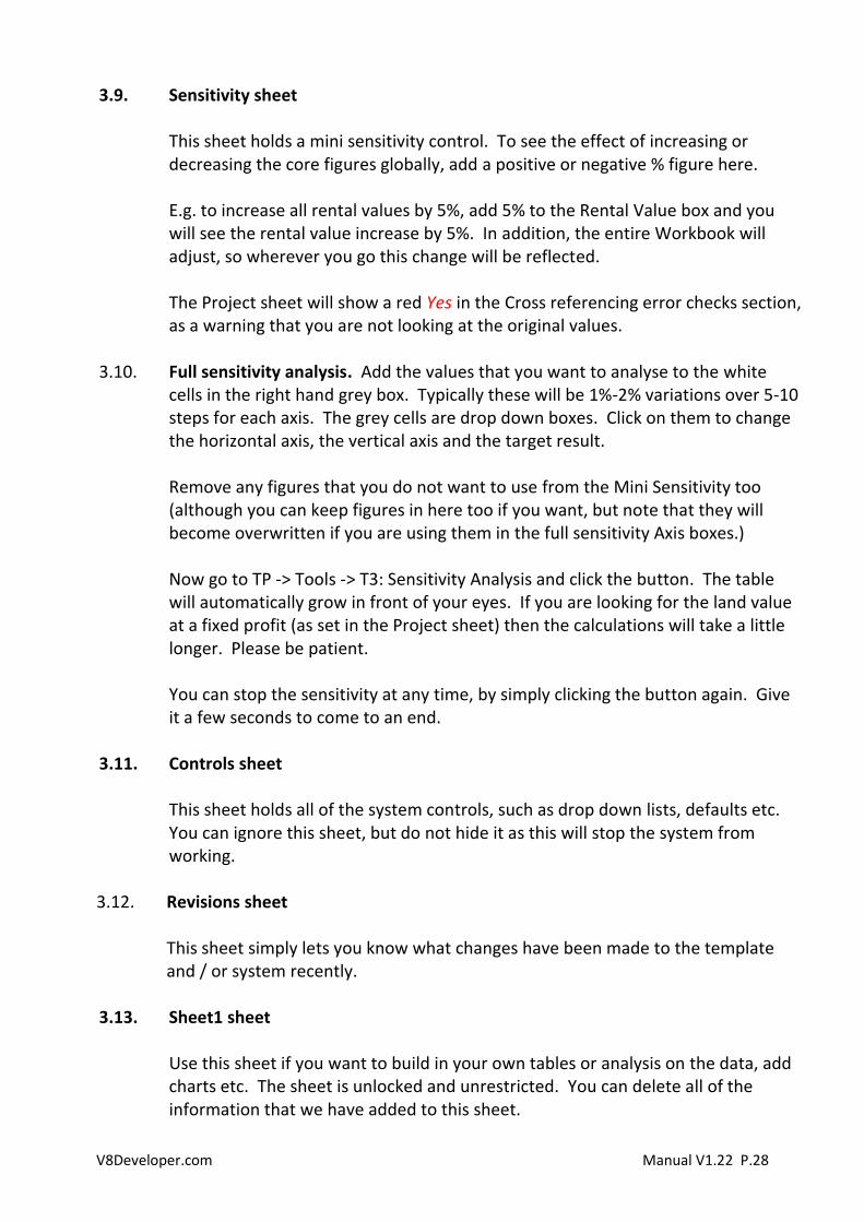
6. Printing / Exporting as PDF You can use the standard printing settings in Excel for printing. If you ‘preview’ your print layout then this will allow you to adjust it. You can also add header and footer information which will print out every time. To do this go to Excel -> File -> Print -> Page Setup (this is in blue at the bottom of the print options)
SAVING AS PDF: If you want to save to a PDF, print preview first to get the output that you want, then go to Excel -> File -> Save as -> Browse. Change the ‘Save as Type’ drop down to PDF (towards the bottom of the list.) At this point you can click ‘Options’, to change what is saved. Then save the file. This will then save as per your print setting.
V8Developer.com Manual V1.22 P.30
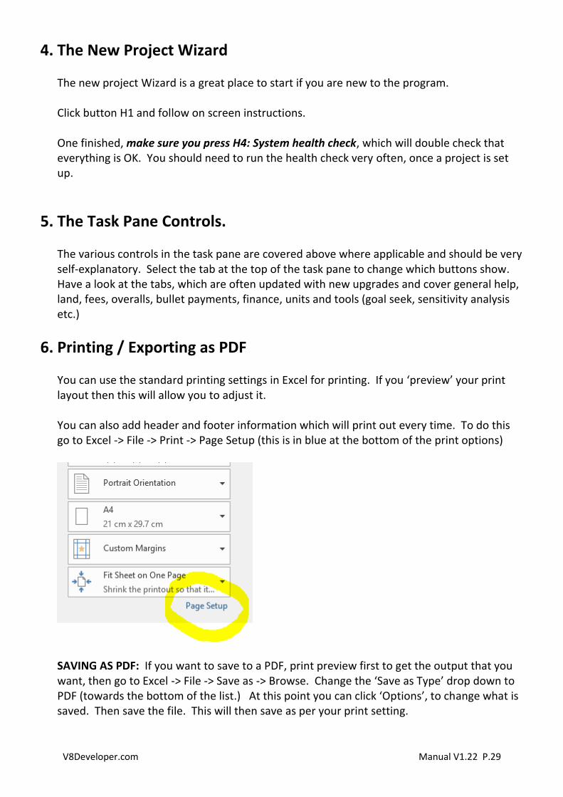
Colour Printing If you want to print in colour do the following from a PC. Mac will vary slightly.
7. Troubleshooting. Please see the following page on our website: http://caldes.com/h-troubleshooting