Calculus III Final Project - Mathematical Paper (100 points)

You must research a specific application(s) that uses one or more of the major theorems of vectorcalculus. This should be chosen, discussed with me, and approved by Tuesday 4-27-21.

You will write a minimum six page, typed, single spaced paper (not including references or images) thatincludes:

Section 1. IntroductionAn expository overview of the mathematics and of your application (mostly verbal with minimal mathand technical details).

Section 2. Technical Details of the Mathematics (only)A purely mathematical discussion of this mathematics, including simple (toy) explanatory mathematicalexamples.

Section 3. Technical Details of the Application(s) of your mathematics in Section 2.Describe the technical mathematical details of examples of your specific, interesting, realapplication(s).

Section 4. Conclusion.Summarize your work in Sections 2 & 3 and write a conclusion.

References.The following mathematical format must be used:Kurt Gödel, "An Example of a New Type of Cosmological Solution of Einstein's Field Equations ofGravitation", Rev. Mod. Phys. 21, 447, 1949.

Math formulas must be typeset - you can use the free Latex at https://www.overleaf.com/

You must fulfill daily progress milestones each class period – 5 points each on Infinite Campus.Milestone 0. Due 4-27-2021: Approval of your project mathematics and application area.Milestone 1. Due 4-29-2021: A detailed outline of your paper.Milestone 2. Due 5-04-2021: A rough draft of section 1.Milestone 3. Due 5-06-2021: A rough draft of section 2.Milestone 4. Due 5-11-2021: A rough draft of section 3.Milestone 5. Due 5-13-2021: A final version of sections 1 & 2.Milestone 6. Due 5-14-2021: A final version of sections 3, including conclusion and references.

Presentation Day 1. 5-14-2021: Seniors will present their papers to the class (10-15 min each).

Presentation Days 2 & 3. 5-27,28-2021: Non seniors will present their papers to the class.

Your Final Project grade will be based on the depth and interest of your choice of mathematics

and the development of your application, and on the quality of your writing, including the

professional formatting of your paper.

Note. You must meet the following schedule whether or not you attend class. You must email me the information for the daily milestone, even if you miss class through an excused absence.

Fluid Simulation with the Navier-Stokes Equations

Audrey Wang

May 4, 2018

1 Introduction

The extraordinary advances in computer graphics over the past century have allowed us togenerate hyper-realistic simulations of the world behind our digital screens. Engineeringapplications facilitate invaluably fast visualization of newly designed shapes. Increasinglydetailed simulators and imaging tools graphically illustrate scientific and medical datato enable researchers to understand, illustrate, and glean insight from their results. CGItools help entertainment media create unbelievably immersive experiences, giving riseto realistic special effects and gorgeous fantasy worlds—and in the case of video games,worlds that players can interact with.

These advances have been no easy feat, requiring the imagination and ingenuity ofmany talented and dedicated individuals. And one aspect of the real world has beenespecially difficult to translate to computer graphics: fluid dynamics, or how fluids move.Fluid flows are everywhere: from rising smoke, mist, and clouds, to the movement ofrivers and oceans. Unlike solids, which can be dealt with as single, rigid objects, movingfluids have differential volumes with varying velocities, and thus must be represented withvector fields for accurate computational results. When considering the change in thesevector fields over time, vector calculus comes into play.

In this paper, our goal is to explore a way to create accurate, practical fluid simula-tions for graphical implementation, and also to understand the mathematics behind themethod. We will first familiarize ourselves with the basic vector calculus concepts neces-sary for creating fluid simulations. The section after that will introduce the infamouslycomplex equations that serve as the basis for our understanding of viscous fluid dynamics:the Navier-Stokes equations. In order to deepen our understanding of fluid dynamics, wewill derive the Navier-Stokes equations and explain the significance of its components.Finally, we will look at an example of how to use the Navier-Stokes equations to programan actual fluid simulator.

1.1 Vector Calculus Concepts

Vector fields map each point in space to a vector. In the context of fluid dynamics,the value of a vector field at a point can be used to indicate the velocity at that point.Much of vector calculus uses the del operator, represented by the nabla symbol ∇. Inreal three-dimensional space with i, j, and k denoting the unit vectors for the coordinateaxes, the del operator is defined as:

∇ = i∂

∂x+ j

∂

∂y+ k

∂

∂z

1

The following are definitions of differential operators that we will later use in theNavier-Stokes equations [1]:

Gradient

grad(f) = ∇f =∂f

∂xi +

∂f

∂yj +

∂f

∂zk

Divergence

divF = ∇ · F =

(∂

∂x,∂

∂y,∂

∂z

)· (Fx, Fy, Fz) =

∂Fx∂x

+∂Fy∂y

+∂Fz∂z

Curl

∇ × F =

∣∣∣∣∣∣i j k∂∂x

∂∂y

∂∂z

Fx Fy Fz

∣∣∣∣∣∣Laplacian

∇f = ∇2 = (∇ · ∇)f =∂2f

∂x2+∂2f

∂y2+∂2f

∂z2

1.1.1 Divergence Theorem

Another important concept from vector calculus that we’ll use in this paper is the di-vergence theorem, also known as Gauss’ Divergence Theorem, which states that, given asimple solid region W with a positive orientation and a boundary region S:

ˆ ˆ ˆW

∇ · FdV =

ˆ ˆS

F · dS

This means that the divergence of F through W equals the flux of F through the boundarysurface S enclosing W.

1.2 The Navier-Stokes Equations

The Navier-Stokes equations, developed by Claude-Louis Navier and George GabrielStokes in 1822, are essential to the field of computational fluid dynamics. They canbe used to determine the velocity vector field that applies to a viscous fluid, given someinitial conditions. They arise from the application of Newton’s second law in combinationwith a fluid stress (due to viscosity) and a pressure term. These equations, however, canbe solved analytically only for a few very simple physical configurations. Usually, theyresult in a system of extremely complex partial differential equations that are difficult orimpossible to solve [2]. However, it is possible to use numerical integration techniques(along with computer assistance) to estimate approximate solutions. In the next section,we will go through the derivation of the Navier-Stokes equations in their entirety andthen take a look at a simple configuration for which an exact solution is available.

2

2 Deriving the Navier-Stokes Equations

2.1 Background

Before we begin deriving the Navier-Stokes Equations, we must first familiarize ourselveswith some basic concepts of fluid dynamics. The first is the distinction between intensiveand extensive properties. Intensive properties are ones whose values do not depend onthe volume of measurement (e.g. pressure, density, momentum, velocity). Extensiveproperties do depend on the volume of measurement (e.g. mass, volume, surface area).Intensive properties can be evaluated generally on differential elements, and thus will bethe focus in this derivation.

Second, we require the continuum hypothesis of fluid dynamics, which is the assump-tion that the properties of a fluid can be described by continuous functions [3]. Thisassumption allows us to ignore the fact that the fluid is made of trillions of discrete par-ticles, instead allowing us to represent intensive properties in a mathematically coherentway on the macroscopic level.

One final concept we’ll use to derive the equations is the assumption of an incom-pressible, homogeneous fluid. A fluid is incompressible if the volume of any subregionof the fluid is constant over time. A fluid is homogeneous if its density is constant inspace. A fluid that is incompressible and homogenous has constant density in both timeand space. These assumptions are common in fluid dynamics; they simplify calculationswhile still preserving the applicability of the resulting mathematics to fluid simulations[2].

2.2 Mass Continuity Equation

With these assumptions in place, we can finally begin the actual mathematical derivation.The first thing we’ll need is the conservation of mass, which states that, given an isolatedsystem, the amount of matter remains constant over time. Let us apply this law to afluid with an arbitrary volume V , surface ∂V , and surface element dA. On dA, densityρ and velocity u are constant. The mass flow rate equation [4] tells us that density timesvelocity times area is equal to the amount of mass M that flows through that area overtime t, or M/t = ρuA when density and velocity are constant. Since density and velocityare only constant over a differential surface element dA, the form of this equation weneed is

dM

dt= ρu · dA, or

dM

dt= ρu · ndA,

where n is the outward unit normal to dA.If we integrate over the surface, we find that the total mass flux across ∂V is equal to

the rate of change of the mass within V :

dM

dt= −

ˆ ˆ∂V

ρu · ndA.

By the divergence theorem, this equation can also be written as

dM

dt= −

ˆ ˆ ˆV

(∇ · (ρu))dV.

3

The triple integral of a density function over a volume is the mass of that volume, orM =

´ ´ ´Vρ · dV , so dM

dt=´ ´ ´

VdρdtdV . Thus −

´ ´ ´V

(∇ · (ρu))dV =´ ´ ´

VdρdtdV ,

or

0 =

ˆ ˆ ˆV

(dρ

dt+ (∇ · (ρu))

)dV.

This is true for every V , so the integrand must equal zero. Thus we arrive at the masscontinuity equation,

dρ

dt+ (∇ · (ρu)) = 0.

Since we can assume incompressibility, we can say that the density is constant. Thederivative of a constant is zero, so after dividing both sides by ρ, the mass continuityequation can then simplify to

∇ · u = 0.

2.3 Cauchy Momentum Equation

The mass continuity equation, which applies the conservation of mass, is only one partof the Navier-Stokes Equations. The bulk of the math actually comes in the derivationand application of the Cauchy momentum equation, which applies the conservation ofmomentum and governs momentum transport. This section references and modifies thederivation by Neal Coleman [5].

We start the derivation by considering an incompressible, viscous fluid filling Rn

subject to an external body force f , which is a time-variant vector field f : Rn ×[0,∞)→ Rn. Force components are denoted by fi (with i being the direction of the forcecomponent). Consider a volume element dV in Rn. The total body force acting in the xidirection on dV is due to force component fi and forces caused by the stress tensor σij.The component σij represents the force per unit area in the xi direction acting on a pointon a plane cut through Rn with normal in the xj direction. There are n directions xj,and each σij component varies by some small amount, ∂σij, in each of those directions.

Each differential volume dV has side lengths dxi, so the rate of stress variation is∂σij∂xi

.Thus, the total force on dV in the xi direction (the body force times the volume) is:

Fi = fidV +∑j

∂σij∂xj

dV.

Next, we can apply some basic equations of motion. We know the equations ofmomentum and force: P = mu (P is momentum, m is mass, and u is velocity) andF = ma (F is force and a is acceleration). For a differential volume element dV ,m = ρdV , so the momentum in the xi direction is Pi = ρuidV . Also, a = u

t, so

F = Pt, or F = dP

dt. Thus, we can differentiate momentum with respect to time, using

the chain rule and noting that each xi is a function of time and uj = dxidt

:

dPidt

=d

dt(ρuidV ) = ρ

(∂ui∂t

+∑j

uj∂ui∂xj

)dV.

Setting this equal to the previous Fi expression and integrating over arbitrary volumeΩ, we get:

4

ˆΩ

(fi +

∑j

∂σij∂xj

)dV =

ˆΩ

ρ

(∂ui∂t

+∑j

uj∂ui∂xj

)dV.

Equivalently,

ˆΩ

[(fi +

∑j

∂σij∂xj

)− ρ

(∂ui∂t

+∑j

uj∂ui∂xj

)]dV = 0.

The integrand must be zero. Thus, we have arrived at the Cauchy momentum equa-tion:

fi +∑j

∂σij∂xj

= ρ

(∂ui∂t

+∑j

uj∂ui∂xj

).

In order to simplify this equation to a version applicable for fluids, we must make somedefinition for the stress tensor, σij. We can assume that the stress on a given volumeelement is related to the velocity gradient. For example, consider a simple, unidirectionalstream of water where flow speed is related to its height y from the bottom. This fluidwill begin to shear as the top flows more quickly than the bottom. In this scenario, stresscan be defined as

σ = νdu

dy,

where ν is a proportionality constant known as viscosity.Generally, the stresses acting on a fluid element dV can be represented in two compo-

nents. The first is a normal uniform stress, known as pressure (p), which is the averageof all the normal stresses:

p =−∑σii

n.

The second component is a deviatoric stress τij = σij − pδij, composed of the non-normal stress components sigmaij and the deviation of the normal stresses from thepressure. The deviatoric stress deforms dV . For a better visualization of what the stresstensor is, consider this matrix representation in R3:

σ =

σxx τxy τxzτyx σyy τyzτzx τzy σzz

The deviatoric stress tensor can also be expressed as τij = 2µeij, where eij is the rate

of strain tensor eij = 12( ∂ui∂xj

+∂uj∂xi

). These additional elements—pressure, viscosity, and

stress tensors—allow us to simplify the Cauchy momentum equations into the followingform:

∂u

∂t= −(u · ∇)u − 1

ρ∇p + ν∇2u + F,

using the definitions of del operators listed in Section 1.1. For the full, step-by-stepsimplification, see [5].

5

2.4 Full Equations and Explanation

We can thus describe the state of a fluid over time by the Navier-Stokes equations forincompressible flow:

∇ · u = 0 (1)

∂u

∂t= −(u · ∇)u − 1

ρ∇p + ν∇2u + F (2)

Equation 1 is the mass continuity equation, and equation 2 is the Cauchy momentumequation, where u is the fluid’s velocity field, ρ is the (constant) fluid density, p is thescalar pressure field, ν is viscosity, and F represents any external forces that act on thefluid. Solving the equations requires solving for u and p, which are unknown quantitiesthat vary over time. Each of the terms in the Cauchy momentum equations represents adifferent physical property involved in the movement of the fluid. The term −(u · ∇)u iscalled the advection term. It represents how the velocity of the fluid carries itself alongand moves the liquid velocities. The term −1

ρ∇p is the pressure term, and it represents

how the liquid particles move in response to changing pressure, specifically how particlesmove from high to low pressure. The third term, ν∇2u, is the diffusion term, and dealswith the effects of viscosity. Viscosity is a measure of a liquid’s resistance to flow. Thisresistance results in the diffusion of momentum (and therefore velocity). The final term,F , simply represents acceleration due to external forces; both body forces like gravity,which apply to the whole body of liquid, and local forces like wind, which only affectspecific regions of the liquid.

3 Applying the Navier-Stokes Equations to Program

a Fluid Simulator

As we’ve established, it’s extremely difficult to solve the Navier-Stokes equations for exactsolutions in most situations. However, with the aid of a proper computer algorithm, wewill be able to approximate needed values over time increments in order to generate arealistic fluid simulation. In this section, we’ll look at a simple way to create a 3D fluidsimulation in a fluid cube.

The first step to using the Navier-Stokes equations in an actual fluid simulation ap-plication is to transform the equations into a form more suitable for numerical solutions.The common form of the equations does not readily reveal a method to solve for u or p,and involves two equations. The following transformation results in a single equation forvelocity that can be more readily implemented in an algorithm, along with some simplersteps integral to the algorithm.

3.1 Helmholtz-Hodge Decomposition

The Helmholtz-Hodge decomposition theorem states that a vector field w on D can beuniquely decomposed in the form:

w = u + ∇p,

6

where u has zero divergence and is parallel to ∂D [6]. Equivalently, u = w − ∇p.Taking the divergence of both sides, we have ∇ · w = ∇ · (u + ∇p) = ∇ · u + ∇2p.Since ∇ · u = 0, we obtain

∇2p = ∇ ·w.

This equation is a Poisson equation (see [7]), and it gives us a method to computethe pressure field p. We’ll need to solve for w, our divergent velocity, use the Poissonequation to solve for p, and then use the Helmholtz-Hodge decomposition to finally arriveat u.

To solve for w, we can define an operator P that projects any vector field w ontoits divergence-free component u = Pw. Applying this operator to both sides of theHelmholtz-Hodge decomposition yields Pw = Pu + P(∇p). But by the definition ofthe operator, Pw = Pu = u. Thus, P(∇p) = 0. Now, applying the operator to theNavier-Stokes equations, we have

P∂u

∂t= P

(− (u · ∇)u− 1

ρ∇p+ ν∇2u + F

).

Finally, this simplifies down to

∂u

∂t= P(−(u · ∇)u + ν∇2u + F). (3)

This is a single equation for velocity and represents the entire algorithm we will imple-ment. Now, we can move on to the actual algorithm.

3.2 Algorithm

I will go over the general algorithm supplemented with some examples of pseudocode (inJava) for a better idea of implementation. First, we can create a class that representsthe body of fluid we’ll create and run our simulation on. Let’s call this class FluidCube.Here is an example of how to set up the class, with some private instance variables anda constructor shown:

public class FluidCube

private int size;

private double timeStep;

private double viscosity;

private double density;

private boolean simulating;

private double[][][] cube;

public FluidCube(int size, double timeStep, double viscosity, double density,

boolean simulating, double[][][] velocityGrid)

this.size = size;

cube = velocityGrid.clone();

this.timeStep = timeStep;

this.viscosity = viscosity;

this.density = density;

7

this.simulating = simulating;

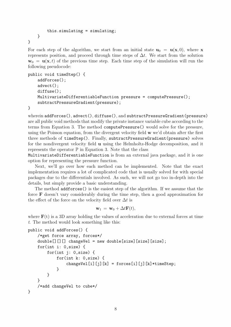
For each step of the algorithm, we start from an initial state u0 = u(x, 0), where xrepresents position, and proceed through time steps of ∆t. We start from the solutionw0 = u(x, t) of the previous time step. Each time step of the simulation will run thefollowing pseudocode:

public void timeStep()

addForces();

advect();

diffuse();

MultivariateDifferentiableFunction pressure = computePressure();

subtractPressureGradient(pressure);

wherein addForces(), advect(), diffuse(), and subtractPressureGradient(pressure)

are all public void methods that modify the private instance variable cube according to theterms from Equation 3. The method computePressure() would solve for the pressure,using the Poisson equation, from the divergent velocity field w we’d obtain after the firstthree methods of timeStep(). Finally, subtractPressureGradient(pressure) solvesfor the nondivergent velocity field u using the Helmholtz-Hodge decomposition, and itrepresents the operator P in Equation 3. Note that the classMultivariateDifferentiableFunction is from an external java package, and it is oneoption for representing the pressure function.

Next, we’ll go over how each method can be implemented. Note that the exactimplementation requires a lot of complicated code that is usually solved for with specialpackages due to the differentials involved. As such, we will not go too in-depth into thedetails, but simply provide a basic understanding.

The method addforces() is the easiest step of the algorithm. If we assume that theforce F doesn’t vary considerably during the time step, then a good approximation forthe effect of the force on the velocity field over ∆t is

w1 = w0 + ∆tF(t),

where F(t) is a 3D array holding the values of acceleration due to external forces at timet. The method would look something like this:

public void addForces()

/*get force array, forces*/

double[][][] changeVel = new double[size][size][size];

for(int i: 0,size)

for(int j: 0,size)

for(int k: 0,size)

changeVel[i][j][k] = forces[i][j][k]*timeStep;

/*add changeVel to cube*/

8

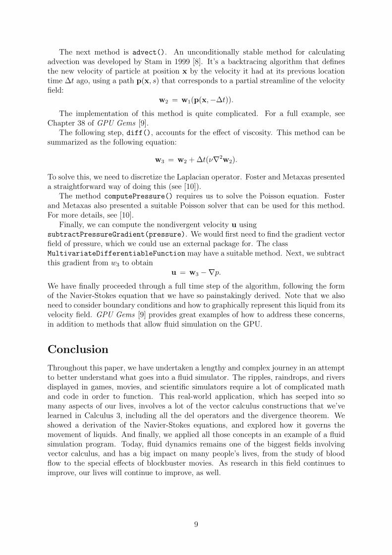
The next method is advect(). An unconditionally stable method for calculatingadvection was developed by Stam in 1999 [8]. It’s a backtracing algorithm that definesthe new velocity of particle at position x by the velocity it had at its previous locationtime ∆t ago, using a path p(x, s) that corresponds to a partial streamline of the velocityfield:

w2 = w1(p(x,−∆t)).

The implementation of this method is quite complicated. For a full example, seeChapter 38 of GPU Gems [9].

The following step, diff(), accounts for the effect of viscosity. This method can besummarized as the following equation:

w3 = w2 + ∆t(ν∇2w2).

To solve this, we need to discretize the Laplacian operator. Foster and Metaxas presenteda straightforward way of doing this (see [10]).

The method computePressure() requires us to solve the Poisson equation. Fosterand Metaxas also presented a suitable Poisson solver that can be used for this method.For more details, see [10].

Finally, we can compute the nondivergent velocity u usingsubtractPressureGradient(pressure). We would first need to find the gradient vectorfield of pressure, which we could use an external package for. The classMultivariateDifferentiableFunction may have a suitable method. Next, we subtractthis gradient from w3 to obtain

u = w3 −∇p.

We have finally proceeded through a full time step of the algorithm, following the formof the Navier-Stokes equation that we have so painstakingly derived. Note that we alsoneed to consider boundary conditions and how to graphically represent this liquid from itsvelocity field. GPU Gems [9] provides great examples of how to address these concerns,in addition to methods that allow fluid simulation on the GPU.

Conclusion

Throughout this paper, we have undertaken a lengthy and complex journey in an attemptto better understand what goes into a fluid simulator. The ripples, raindrops, and riversdisplayed in games, movies, and scientific simulators require a lot of complicated mathand code in order to function. This real-world application, which has seeped into somany aspects of our lives, involves a lot of the vector calculus constructions that we’velearned in Calculus 3, including all the del operators and the divergence theorem. Weshowed a derivation of the Navier-Stokes equations, and explored how it governs themovement of liquids. And finally, we applied all those concepts in an example of a fluidsimulation program. Today, fluid dynamics remains one of the biggest fields involvingvector calculus, and has a big impact on many people’s lives, from the study of bloodflow to the special effects of blockbuster movies. As research in this field continues toimprove, our lives will continue to improve, as well.

9

References

[1] Jerrold E. Marsen, Anthony J. Tromba, Vector Calculus: Fifth Edition, W. H. Free-man and Company, 2003.

[2] Andrew Gibiansky, Fluid Dynamics: The Navier Stokes Equations, May 7,2011. http://andrew.gibiansky.com/blog/physics/fluid-dynamics-the-navier-stokes-equations/

[3] Yue-Kin Tsang, Basic Fluid Dynamics, February 9, 2011.

[4] Nancy Hall, Conservation of Mass, https://www.grc.nasa.gov/www/k-12/airplane/mass.html (updated May 05, 2015)

[5] Neal Coleman, A Derivation of the Navier-Stokes Equations, B.S. UndergraduateMathematics Exchange, 7, 20-26 (2010).

[6] A.J. Chorin and J.E. Marsden, A Mathematical Introduction to Fluid Mechanics:3rd ed., Springer, 1993.

[7] Richard Fitzpatrick, Poisson’s equation, February 02, 2006.http://farside.ph.utexas.edu/teaching/em/lectures/node31.html

[8] Jos Stam, Stable Fluids, 1999.

[9] Mark J. Harris, GPU Gems, NVIDIA, 2004.

[10] N. Foster and D. Metaxas, Modeling the Motion of a Hot, Turbulent Gas, ComputerGraphics Proceedings, Annual Conference Series, 181–188, August 1997.

10

Generalizing the Major Theorems of Vector CalculusUsing Differential Forms

Macey Goldstein

May 8, 2018

1 Introduction and Review

1.1 The Applications and Shortcomings of Vector Calculus

Vector calculus is useful for a great many things. Theorems such as the FundamentalTheorem of Calculus for Line Integrals, Greens’ Theorem, Stokes’ Theorem, and Gauss’ Di-vergence Theorem (all of which are written explicitly below) not only make calculations eas-ier; they have also paved the way for a number of practical applications. Vector calculus hasextensive applications in fields like engineering and physics to describe concepts includingfluid dynamics, electromagnetism, and gravitational fields.

Greens’ Theorem:ÏD

(∂Q

∂d x− ∂P

∂d y)d A =

˛

C

Pd x +Qd y

Stokes’ Theorem:ÏS

(∇×F) ·dS =˛

C

F ·ds

Gauss’ Divergence Theorem:Ñ

R

(∇·F)dV =ÏS

F ·dS

Fundamental Theorem of Calculus for Line Integrals:

ˆc

∇ f ·ds = f (c(b))− f (c(a))

However, vector calculus’ offerings can be somewhat limited if we want to expand ourunderstanding outside the x y z-plane. The reason we want to expand concepts from vectorcalculus is that we would ideally want to see that they "work" outside of human constructs,like coordinate systems. For example, as one progresses down the middle two equationslisted above, he or she may note that each is simply a generalization of that which precededit. (i.e. Stokes’ Theorem generalizes Greens’ Theorem from R2 to R3 and Gauss’ DivergenceTheorem generalizes Stokes’ Theorem from describing surfaces and their boundaries to de-scribing regions and their boundaries). However, it would be very difficult to generalizethese equations any further using vector calculus. It would be much simpler to use anothermethod to do this. The method that mathematicians use to escape the confines of definedcoordinate planes is by using differential forms. This paper will work toward and culminatein the generalization of many of the major theorems of vector calculus, by showing that theycan all be derived from one other, more general equation.

1

1.2 A Review of Differential Forms

For now, let us provide a brief explanation of what a differential form is. The most ba-sic definition of a form is an object which acts on vectors and returns a number value. Adifferential form is a special case of a form, in which the forms are both continuous anddifferentiable.

Figure 1: The line l exists within R2 in a plane defined by the curve and the point at which lis tangent to the curve. The equation of the line at point (1,1) is d y = 2d x.

The reason we use forms is that they allow us to transcend the confines of specifically-defined coordinate systems, (e.g. the Euclidean coordinate system). Rather, forms allow usto base our coordinate system on a point on a curve. An example of a differential form maylook like this:

ω= f1(x, y, z)d x + f2(x, y, z)d y + f3(x, y, z)d z.

We would call this a 1-form, because it takes one vector. An important thing to rememberabout forms is that we often define them as specific n-forms. For example, the exampleabove was a 1-form, and the examples below are a 0-form, 2-form, and 3-form respectively.In these examples, all of the forms are on R3. (Notice that a 0-form looks the same as amultivariable function. It can be represented as such in the context of forms.)

• 0-form: ω= f (x, y, z)

• 2-form: ω= f1(x, y, z)d x ∧d y + f2(x, y, z)d y ∧d z + f3(x, y, z)d z ∧d x

• 3-form: ω= f (x, y, z)d x ∧d y ∧d z

The symbol ∧ denotes the "wedge" product, which is the multiplication operator equiv-alent for forms. The wedge product can be thought of conceptually in a number of ways,including as the sum of the areas of parallelograms formed (on different planes) by the in-put vectors of the function multiplied by a constant. However, most of these conceptual-izations delve far deeper into the specifics of the wedge product than are necessary for this

2

discussion. For our purposes, it will be sufficient to simply think of it as an analogue of themultiplication operator for differential forms. We will discuss the wedge product more inthe proceeding section.

Although working with 1- and 2-forms has a lot of advantages, in order to truly generalizeanything, we would like to think of all forms as n-forms, without explicitly defining whichinteger n is for each form. We want our equations to work for the broadest range of possibleforms. We will eventually be attempting to integrate n-forms over the sets of real numbersRn and Rm . n-forms will look like this:

n-form: ω= f (x1, x2, . . . , xn)d x1 ∧d x2 ∧ . . .∧d xn .

1.3 A Review of the Wedge Product

Before we continue, it is important that we understand a little bit more about the wedgeproduct. Although a comprehensive definition of the wedge product will not be offered inthis paper, it is important that readers are familiar with some of its basic identities. Someimportant identities are listed below.

• The result "wedging" an n-form with itself is 0. (e.g. ω∧ω= 0)

• The wedge product is distributive. (e.g. ω∧ (ν+η) =ω∧ν+ω∧η)

• The wedge product is multilinear. (e.g. cω∧ν= c(ω∧ν) =ω∧ cν)

• The wedge product is alternating. (e.g. ω∧ν=−ν∧ω, ω∧ν∧η=−ω∧η∧ν)

1.4 A Review of Differentiating and Integrating Differential Forms

In this section, we will briefly discuss some of the important features of differentiatingand integrating differential forms. As in the previous section, we will forego some of theintricacies of this topic, as it is not the purpose of the paper. The goal of this section, rather,is to provide context, as we will need to both differentiate and integrate forms in the courseof this paper.

• Differentiating 0-forms: d f (x1, x2, . . . , xn) = ∂ f∂x1

d x1 + ∂ f∂x2

d x2 + . . . ∂ f∂xn

d xn

• Differentiating n-forms: dω= d f (x1, x2, . . . xn)∧ d x1 ∧ d x2 ∧ . . .∧d xn

• Differentiating the derivatives of differential forms: d(dω) = 0

• Integrating n-forms over Rn :´

f (x1, x2, . . . xn)d x1∧d x2∧ . . .∧d xn = ´ f d x1d x2 . . .d xn

• Integrating n-forms with parameterization φ(x1, x2, . . . xn) :Rm →Rn over Rm :´Rnω= ´

Rmω(φ(x1, x2, . . . , xn) · ( ∂φ∂x1

(x1, x2, . . . , xn), . . . ( ∂φ∂xn(x1, x2, . . . , xn)

3

2 Generalizing Stokes’ Theorem Using Differential Forms

2.1 Cells

We will now begin our discussion with a quick overview of cells and chains. Cells are asubset of the region Rm , whose boundaries are defined in each dimension n. So, each n-cell(as they are often called) takes in input of n dimensions and projects an image onto the seatof real numbers Rm . We define 0-cells as points on Rm .

The cell σ is the image of the parameterization φ : I n → Rm , where I n is the set of realnumbers within Rm from [a,b], and a and b are the limits of the domains of each dimensionin Rm .

2.2 Boundaries of n-cells

Equally important to defining n-cells is defining the boundaries of those chains. We de-note the boundary of the n-cell σ as ∂σ. If there exists a parameterization φ for σ, we definethe boundary of this cell as the alternating sum of all the combinations of input variablesand limits for φ. The boundaries of three cells are shown below. The first is a 1-cell withlimits [a,b] and a parameterization φ(x); the second is a 2-cell with limits [a,b]× [c,d ] anda parameterization φ(x, y); and the third is a 3-cell with limits [a,b]× [c,d ]× [g ,h]. and aparameterization φ(x, y, z)

• Boundary of a 1-cell: ∂σ1 =φ(b)−φ(a)

• Boundary of a 2-cell: ∂σ2 = (φ(b, y)−φ(a, y)− (φ(x,d)−φ(x,c))

• Boundary of a 3-cell: ∂σ3 = (φ(b, y, z)−φ(a, y, z))− (φ(x,d , z)−φ(x,c, z))+ (φ(x, y,h)−φ(x, y, g ))

2.3 Chains and Their Boundaries

A chain is a linear combination of cells. Essentially, chains are the sum or difference ofmultiple cells, or the product of a cell and a coefficient. They help us define broader regionsthan cells alone can. The definition for chains and for the integrals of forms over chains canbe found below.

• The chain C is: C = n1σ1 +n2σ2 + . . .+nnσn , where each n represents the coefficientfor the term and each σ represents a distinct n-cell.

• The integral of an n-form over an n-chain is:´Cω= n1

´σ1

ω+n2´σ2

ω+ . . .+nn´σn

ω.

All of the same identities apply to the boundaries of n-chains. We simply replace the cellσ with its boundary ∂σ.

• The boundary of the chain C is: ∂C = n1∂σ1 +n2∂σ2 + . . .+nn∂σn .

• The integral of an n-form over an n-chain is:´∂Cω= n1

´∂σ1

ω+n2´∂σ2

ω+ . . .+nn´∂σn

ω

4

2.4 Putting It All Together

Now, having defined forms (a general way of conceptualizing functions in n- and m-space) and chains (a general description of regions in n- and m-space), we are ready todefine the general equation that we have been building up to. The full proof for the Gener-alized Stokes’ Theorem requires even more prerequisite understanding of n- and m-space,including an understanding of objects called manifolds. However, we can offer a definitionof this important theorem that applies to the cells and chains that we have defined.

We will begin by defining a region of space R (a 3-cell) with limits [a,b] on x, [c,d ] on y ,and [g ,h] on z. Next, we will define a 2-form ω, whose derivative we can integrate over theregion R. The 2-form we will choose is: ω= f (x, y, z)d y ∧d z. Given our knowledge of forms,

we can then see that dω= ∂ f∂x d x ∧d y ∧d z.

In order to calculate´R

dω, we will define three vectors over which we will integrate. The

vectors we choose are V1 = ⟨b −a, y, z⟩,V2 = ⟨x,d − c, z⟩, and V3 = ⟨x, y,h − g ⟩. Our next stepis to use these vectors to determine the value of dω(V1,V2,V3). After that we will find theRiemann Sums for each dimension of the region R and take the limit of that sum until thedistances between the limits in each dimension are infinitesimally small.

At this point, it will be useful to step back and take a look at the bigger picture, as far aswhat is going on thus far. For our purposes, we can think of the region R as a rectangularprism, because the x,y , and z directions all increase in a linear manner between two values.The volume of that prism, then, is the value of d x ∧d y ∧d z(V1,V2,V 3). If we imagine anorientation such that the x-direction is vertical, we can define the height s to be the magni-tude of V1. Another definition we have for s (and a more useful one, at that) is the differenceof the points p(b, y, z) and p(a, y, z). The area of the prism’s base, then, would be equal tod y ∧d z(V2,V3). Thus, we can come up with the identity listed below.

VolumeR = d x ∧d y ∧d z(V1,V2,V3) = sd y ∧d z(V2,V3)

Additionally, we can think of the difference between points p(b, y, z) and p(a, y, z) as thevalue s, we can use the definition of a derivative to show that the following holds.

∂ f

∂x(x, y, z)

∣∣∣b

a= lim

s→0

f (b, y, z)− f (a, y, z)

s

Because we will be taking the limit of the difference between the endpoints of each di-

mension later, we will for now use the approximation ∂ f∂x (x, y, z) ≈ f (b,y,z)− f (a,y,z)

s . We cannow see that:

dω(V1,V2,V3) = ∂ f

∂xd x ∧d y ∧d z(V1,V2,V3)

= ∂ f

∂xsd y ∧d z(V2,V3)

≈ f (b, y, z)− f (a, y, z)

ssd y ∧d z(V2,V3)

= f (b, y, z)d y ∧d z(V2,V3)− f (a, y, z)d y ∧d z(V2,V3).

If we remember that we initially defined ω to be equal to f (x, y, z)d y ∧d z, we will dis-cover that:

5

dω=ω(V2(b, y, z),V3(b, y, z)−ω(V2(a, y, z),V3(a, y, z)

We had said that the next step was to take the Riemann Sum of the result. The RiemannSum of the first term,

∑y,zω(V2(b, y, z),V3(b, y, z)), represents the integral of ω over the top of

the prism. The Riemann Sum of the second term,∑y,zω(V2(a, y, z),V3(a, y, z)), represents the

integral of ω over the bottom of the prism. Additionally, if we integrated ω over any pair ofvectors on the other four faces of the cube, the value of those integrals would be 0.

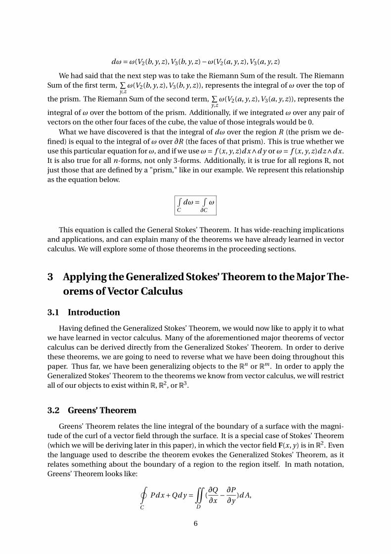
What we have discovered is that the integral of dω over the region R (the prism we de-fined) is equal to the integral of ω over ∂R (the faces of that prism). This is true whether weuse this particular equation forω, and if we useω= f (x, y, z)d x∧d y orω= f (x, y, z)d z∧d x.It is also true for all n-forms, not only 3-forms. Additionally, it is true for all regions R, notjust those that are defined by a "prism," like in our example. We represent this relationshipas the equation below.

´C

dω= ´∂Cω

This equation is called the General Stokes’ Theorem. It has wide-reaching implicationsand applications, and can explain many of the theorems we have already learned in vectorcalculus. We will explore some of those theorems in the proceeding sections.

3 Applying the Generalized Stokes’ Theorem to the Major The-orems of Vector Calculus

3.1 Introduction

Having defined the Generalized Stokes’ Theorem, we would now like to apply it to whatwe have learned in vector calculus. Many of the aforementioned major theorems of vectorcalculus can be derived directly from the Generalized Stokes’ Theorem. In order to derivethese theorems, we are going to need to reverse what we have been doing throughout thispaper. Thus far, we have been generalizing objects to the Rn or Rm . In order to apply theGeneralized Stokes’ Theorem to the theorems we know from vector calculus, we will restrictall of our objects to exist within R, R2, or R3.

3.2 Greens’ Theorem

Greens’ Theorem relates the line integral of the boundary of a surface with the magni-tude of the curl of a vector field through the surface. It is a special case of Stokes’ Theorem(which we will be deriving later in this paper), in which the vector field F(x, y) is in R2. Eventhe language used to describe the theorem evokes the Generalized Stokes’ Theorem, as itrelates something about the boundary of a region to the region itself. In math notation,Greens’ Theorem looks like:

˛

C

Pd x +Qd y =ÏD

(∂Q

∂x− ∂P

∂y)d A,

6

where F(x, y, z) = ⟨P,Q⟩ is a vector field, D is a surface on R2, and C is the boundary of thesurface D . We can choose to represent parts of this equation with differential forms, andwith chains. In order to use the Generalized Stokes’ Theorem to derive Greens’ Theorem, wewill say that Pd x and Qd y are 1-forms. We will also change D to a the 2-chain S and C tothe boundary of that 2-chain: ∂S. Thus, using the Generalized Stokes’ Theorem, we see that:

ˆ

∂S

Pd x +Qd y =ÏS

d(Pd x)+d(Qd y).

By differentiating the two 1-forms, we get:

ÏS

∂P

∂xd x ∧d x + ∂P

∂yd y ∧d x + ∂Q

∂xd x ∧d y + ∂Q

∂yd y ∧d y =

ÏS

(∂Q

∂x− ∂P

∂y)d x ∧d y .

Remembering that d x∧d y = d xd y , we can then rewrite the right side of the equation tomatch our original definition of Greens’ Theorem.

´∂S

Pd x +Qd y =ÎS

(∂Q∂x − ∂P

∂y )d xd y

3.3 The Fundamental Theorem of Calculus

The Fundamental Theorem of Calculus states that the integral of a function f (x), whenevaluated from a to b, is equal to the antiderivative of f (x) evaluated at b minus the an-tiderivative of f (x) evaluated at b.

ˆ b

af ′(x)d x = f (b)− f (a)

One way to arrive at this equation is by thinking of the function f (x) as a 0-form, and of[a,b] as a 1-cell in R. d f , then would be equal to f (x)d x, a 1-form. Therefore:

ˆ b

af ′(x)d x =

ˆ

[a,b]

f ′(x)d x.

By the Generalized Stokes’ Theorem, the integral of the derivative of a form over a cell isequal to the integral of that form over the boundary of that cell, so:

ˆ

[a,b]

f ′(x)d x =ˆ

∂[a,b]

f (x).

If we recall the definition of the boundary of a cell, we remember that it can be thoughtof as the difference between endpoints in a cell. As a result:

ˆ

∂[a,b]

f (x) =ˆ

b−a

f (x).

This integral evaluates the function f (x) from a to b and, as such, can also be representedas:

7

f (x)∣∣∣b

a, which is equal to f (b)− f (a).

Therefore, we can say that the following equation is true.

b

af ′(x)d x = f (b)− f (a)

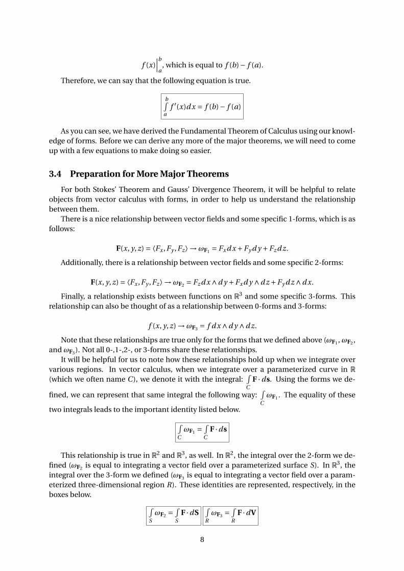
As you can see, we have derived the Fundamental Theorem of Calculus using our knowl-edge of forms. Before we can derive any more of the major theorems, we will need to comeup with a few equations to make doing so easier.

3.4 Preparation for More Major Theorems

For both Stokes’ Theorem and Gauss’ Divergence Theorem, it will be helpful to relateobjects from vector calculus with forms, in order to help us understand the relationshipbetween them.

There is a nice relationship between vector fields and some specific 1-forms, which is asfollows:

F(x, y, z) = ⟨Fx ,Fy ,Fz⟩→ωF1 = Fxd x +Fy d y +Fzd z.

Additionally, there is a relationship between vector fields and some specific 2-forms:

F(x, y, z) = ⟨Fx ,Fy ,Fz⟩→ωF2 = Fzd x ∧d y +Fxd y ∧d z +Fy d z ∧d x.

Finally, a relationship exists between functions on R3 and some specific 3-forms. Thisrelationship can also be thought of as a relationship between 0-forms and 3-forms:

f (x, y, z) →ωF3 = f d x ∧d y ∧d z.

Note that these relationships are true only for the forms that we defined above (ωF1 , ωF2 ,and ωF3 ). Not all 0-,1-,2-, or 3-forms share these relationships.

It will be helpful for us to note how these relationships hold up when we integrate overvarious regions. In vector calculus, when we integrate over a parameterized curve in R

(which we often name C ), we denote it with the integral:´C

F ·ds. Using the forms we de-

fined, we can represent that same integral the following way:´CωF1 . The equality of these

two integrals leads to the important identity listed below.

´CωF1 =

´C

F ·ds

This relationship is true in R2 and R3, as well. In R2, the integral over the 2-form we de-fined (ωF2 is equal to integrating a vector field over a parameterized surface S). In R3, theintegral over the 3-form we defined (ωF3 is equal to integrating a vector field over a param-eterized three-dimensional region R). These identities are represented, respectively, in theboxes below.

´SωF2 =

´S

F ·dS´RωF3 =

´R

F ·dV

8

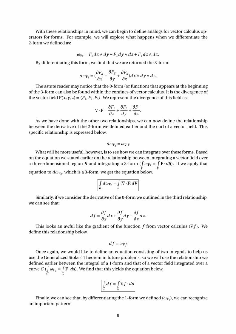
With these relationships in mind, we can begin to define analogs for vector calculus op-erators for forms. For example, we will explore what happens when we differentiate the2-form we defined as:

ωF2 = Fzd x ∧d y +Fxd y ∧d z +Fy d z ∧d x.

By differentiating this form, we find that we are returned the 3-form:

dωF2 = (∂Fx

∂x+ ∂Fy

∂y+ ∂Fz

∂z)d x ∧d y ∧d z.

The astute reader may notice that the 0-form (or function) that appears at the beginningof the 3-form can also be found within the confines of vector calculus. It is the divergence ofthe vector field F(x, y, z) = ⟨F1,F2,F3⟩. We represent the divergence of this field as:

∇·F = ∂F1

∂x+ ∂F2

∂y+ ∂F3

∂z.

As we have done with the other two relationships, we can now define the relationshipbetween the derivative of the 2-form we defined earlier and the curl of a vector field. Thisspecific relationship is expressed below.

dωF2 =ω∇·F

What will be more useful, however, is to see how we can integrate over these forms. Basedon the equation we stated earlier on the relationship between integrating a vector field overa three-dimensional region R and integrating a 3-form (

´VωF3 = ´

VF ·dS). If we apply that

equation to dωF2 , which is a 3-form, we get the equation below.

´R

dωF2 =´R

(∇·F)dV

Similarly, if we consider the derivative of the 0-form we outlined in the third relationship,we can see that:

d f = ∂ f

∂xd x + ∂ f

∂yd y + ∂ f

∂zd z.

This looks an awful like the gradient of the function f from vector calculus (∇ f ). Wedefine this relationship below.

d f =ω∇ f

Once again, we would like to define an equation consisting of two integrals to help ususe the Generalized Stokes’ Theorem in future problems, so we will use the relationship wedefined earlier between the integral of a 1-form and that of a vector field integrated over acurve C (

´CωF1 =

´C

F ·ds). We find that this yields the equation below.

´C

d f = ´C∇ f ·ds

Finally, we can see that, by differentiating the 1-form we defined (ωF1 ), we can recognizean important pattern:

9

dωF1 =∂Fx

∂yd y ∧d x + ∂Fx

∂zd z ∧d x + ∂Fy

∂xd x ∧d y + ∂Fy

∂zd z ∧d y + ∂Fz

∂xd x ∧d z + ∂Fz

∂yd y ∧d z.

By simply moving some of the terms around, we can see a familiar object.

dωF1 = (∂Fy

∂x− ∂Fx

∂y)d x ∧d y + (

∂Fz

∂y− ∂Fy

∂z)d y ∧d z + (

∂Fz

∂x− ∂Fx

∂z)d z ∧d x

dωF1 = (∂Fz

∂y− ∂Fy

∂z)d y ∧d z + (

∂Fx

∂z− ∂Fz

∂x)d x ∧d z + (

∂Fy

∂x− ∂Fx

∂y)d x ∧d y

This result is a 2-form, and it looks very similar to our definition for the curl of a vectorfield. We usually define the curl of a vector field F(x, y, z) = ⟨F1,F2,F3⟩ to be:

∇×F = ⟨∂F3

∂y− ∂F2

∂z,∂F1

∂z− ∂F3

∂x,∂F2

∂x− ∂F1

∂y⟩.

Given the relationship between the curl of a vector field and the derivative of the 1-formwe defined earlier, we can say that the equation below is true.

dωF1 =ω∇×F

And, using the steps we used for the other two dimensions, we can use the relationshipthat we defined at the beginning of this section between the integral of a 2-form and theintegral of a vector field over a surface S (

´SωF2 = ´

SF ·dS) to see that the equation below

holds.

´S

dωF1 =´S

(∇×F) ·dS

Now that we have defined the differential forms that are related to some vector calculusoperators and common integrals, we can begin to apply them to other facets of this field.We will continue to explore how to apply the Generalized Stokes’ Theorem to the major the-orems of vector calculus in the next section.

3.5 Stokes’ Theorem

Stokes’ Theorem is defined as:ÏS

(∇×F) ·dS =˛

C

F ·ds.

The theorem equates the magnitude of the curl of a vector field through a surface withthe line integral around the boundary of that surface. This theorem is itself the generalizedversion of Greens’ Theorem. Whereas Greens’ Theorem applies only for when the vectorfield in question, F(x, y), is defined on R2. Stokes’ Theorem, on the other hand, applies to allfields F(x, y, z) on R3.

Having defined all those relationships in the previous section, one can quickly see thatthe left and right sides of Stokes’ Theorem have equivalent forms. This means that, in orderto derive Stokes’ Theorem, we can convert one side of the equation to the integral of a form.

10

Then we will use the Generalized Stokes’ Theorem. Then we will convert the new integralback into vector calculus terms. Let’s try it. First, we will change the left side of the equationto its equivalent form, remembering the relationships we defined in the previous section.

ˆ

S

(∇×F) ·dS =ˆ

S

dωF1

Next, we will use the Generalized Stokes’ Theorem (´C

dω = ´∂Cω) to change the integral

of the derivative of the form to an integral of the form itself.ˆ

S

dωF1 =ˆ

∂S

ωF1

Finally, we will convert this new integral back into terms from vector calculus by usinganother one of the relationships that we defined earlier.

ˆ

∂S

ωF1 =ˆ

∂S

F ·ds

Thus, we can restate Stokes’ Theorem, now having derived it using differential forms.

´S

(∇×F) ·dS = ´∂S

F ·ds

Hopefully you have noticed that we could have approached this derivation from eitherside of the equation, as we have defined equivalent integrals of differential forms for bothsides. In the next section, we will discuss how to use the Generalized Stokes’ Theorem toderive Gauss’ Divergence Theorem.

3.6 Gauss’ Divergence Theorem

Gauss’ Divergence Theorem is defined as:ÑR

(∇·F)dV =ÏS

F ·dS.

The theorem equates the magnitude of the divergence of a vector field through a three-dimensional region with the magnitude of the flux of that vector field through the surface ofthe region. As Stokes’ Theorem is a generalization of Greens’ Theorem, so too is Gauss’ Di-vergence Theorem a generalization of Stokes’ Theorem. In Stokes’ Theorem relates a curvedefined on R to a defined surface on R2. Gauss’ Divergence Theorem relates a surface de-fined on R2 to a region defined on R3.

We will use the same steps with which we derived Stokes’ Theorem to derive Gauss’ Di-vergence Theorem. If you recall, we began by converting the left side of the equation into anequivalent form integral.

ˆ

R

(∇·F)dV =ˆ

R

dωF2

Next, we will use the Generalized Stokes’ Theorem.

11

ˆ

R

dωF2 =ˆ

∂R

ωF2

Finally, we will convert that equation from the integral of a form to the integral of a vectorfield.

ˆ

∂R

ωF2 =ˆ

∂R

F ·dS

Once again, we can see that we have derived one of the major theorems of vector calculus(this time Gauss’ Divergence Theorem) using differential forms and the Generalized Stokes’Theorem.

´R

(∇·F)dV = ´∂R

F ·dS

3.7 The Fundamental Theorem of Calculus for Line Integrals

The final theorem that we will be deriving is the Fundamental Theorem of Line Integrals.Although this theorem is a form of the Fundamental Theorem of Calculus — which we de-rived earlier by treating f (x, y, z) as a 0-form and d f as a 1-form — we will approach thisderivation a little differently. The Fundamental Theorem of Calculus for Line Integrals isdefined as:

ˆc

∇ f ·ds = f (c(b))− f (c(a)),

where c is a curve on R, with limits from a to b. We will derive this equation much theway we derived the equations for Stokes’ and Gauss’ Divergence Theorems: by using therelationships between vectors and forms that we have already defined, and applying themto this equation. In addition, we will treat c as though it is a 1-cell, and we will say that c isparameterized from a to b by the parameterization φ. We will convert the left side like this:

ˆc

∇ f ·ds =ˆc

d f .

Using the Generalized Stokes’ Theorem, we see that:

ˆc

d f =ˆ

∂c

f .

Because we treat c as a 1-cell, we know that ∂c — the boundary of this 1-cell — is equalto the difference of the endpoints of the cell. (This should be familiar from when we derivedthe Fundamental Theorem of Calculus). Thus:

ˆ

∂c

f =ˆ

b−a

f = f∣∣∣b

a.

When we evaluate f from a to b, by way of the parameterization φ, we see that:

12

f∣∣∣b

a= f (φ(b))− f (φ(a)).

We can now see that we have derived the Fundamental Theorem of Calculus for LineIntegrals.

´c∇ f ·ds = f (φ(b))− f (φ(a))

4 Conclusion

In this paper, we began by reviewing our knowledge of vector calculus. We concludedthat, despite its many applications, there are times when it may be useful to find other so-lutions to a given problem. For the problem of generalizing vector calculus theorems, thatother solution is differential forms. After briefly reviewing some properties of differentialforms, we moved on to the proof of the Generalized Stokes’ Theorem. After this proof, wewere able to use the theorem to derive many equations that we were familiar with from vec-tor calculus. At the conclusion of this paper, it is the author’s hope that his readers will becomfortable using differential forms to express parts of vector calculus.

5 Reference

[1] David Bachman, A Geometric Approach to Differential Forms, Second Edition, 2012

13

Application of the Divergence Theorem and

Stokes’ Theorem to Electricity and Magnetism

Nevan Giuliani

May 2018

1 Introduction

Stokes’ TheoremStokes’ Theorem states that

˜S∇ × ~F · dS =

¸∂S

~F · ds (1). While this mayseem very intimidating, the theorem essentially states that the surface integralof the curl of a vector field is equal to the line integral of the vector field over aclosed path. The theorem has many significant implications across a variety offields including fluid mechanics, thermodynamics, and economics. However, inthis paper we will analyze the application of Stokes’ Theorem to electricity andmagnetism.

Gauss’s LawIn addition to Stokes’ Theorem we will use Gauss’s Law (also known as Gauss’s

Divergence Theorem) which can be written as˝

V∇ · ~F · dV =

˜S~F · dS (2).

The Divergence Theorem implies that the divergence of a vector field over avolume is equal to the flux of the vector field over a surface.

Maxwell’s EquationsMaxwell’s equations are a set of 4 key equations that are crucial to electricityand magnetism. We will derive each one in this paper. In the following equationsB is the magnetic field and E is the electric field.

∇ · E =ρ

ε0

∇ ·B = 0

∇× E = −∂B∂t

∇×B = µ0J + µ0ε0∂E

∂t

1

Ampere’s LawAmpere’s Law allows you use a line integral (often called an Amperian Path)to calculate the magnitude of the magnetic field. It is given by

˛B · ds = µ0Ienc (3)

where B is the magnetic field, µ0 is the permeability of free space, and I is thecurrent enclosed by the surface.

Lorentz ForceThe Lorentz Force Law gives a quantitative way to calculate the force on aparticle due to both electric and magnetic fields. The equation is

~F = q ~E + q~v × ~B (4)

Note that if the particle was not moving ~v = 0, the equation would reduce to~F = q ~E . This implies that a particle must have a nonzero velocity to experiencea magnetic force.

Faraday’s LawFaraday’s Law states that the induced potential difference created by a magneticfield is equal to negative of the time derivative of magnetic flux

V = − d

dt

¨S

B · dS (5)

2 Application

Let’s derive Maxwell’s first equation. As commonly taught in physics, the elec-tric flux through a closed surface is given by

¨S

E · dS =qencε0

(6)

We now define qenc =˝

Vρ dV where ρ is a volumetric charge density.We can

subsitute our expression for the charge into formula (6) to get that

¨S

E · dS =

˝Vρ dV

ε0(7)

Due to the Divergence Theorem we know that˜SE · dS =

˝V∇ · E dV ,

so the right hand side of equation (7) must equal˝

V∇ · E dV . Therefore, we

get ˝Vρ dV

ε0=

˚V

∇ · E dV (8)

2

Moving terms to one side yields˚

V

(∇ · E − ρ

ε0) dV = 0 (9)

Therefore we arrive at the relationship

∇ · E =ρ

ε0(10)

Now, let’s derive Maxwell’s second equation. Due to the fact that magneticmonopoles do not exist, the magnetic flux through a closed surface is 0.

¨S

B · dA = 0 (11)

From the Divergence Theorem we have˜SB · dA =

˝V∇·B dV This yields

˚V

∇ ·B dV = 0 (12)

The final results is∇ ·B = 0 (13)

To derive Maxwell’s third equation we first must start out with Faraday’s Law.This can be written as

V =

¨S

−∂B∂t· dS (14)

Potential Difference over a closed path is also defined as V =´sE · ds. By

Stokes’ Theorem we have´sE · ds =

˜S∇× E · dS. As a result we can set

¨S

−∂B∂t· dS =

¨S

∇× E · dS (15)

Moving terms to one side we get

¨S

(∇× E +∂B

∂t) · dS = 0 (16)

Therefore

∇× E +∂B

∂t= 0 (17)

so

∇× E = −∂B∂t

(18)

To derive Maxwell’s fourth equation we first must start out with Ampere’s Lawwhich gives a relationship between magnetic field and enclosed current.

3

˛s

B · ds = µ0Ienc (19)

We can define Ienc =˜SJ ·dS where J is a current density. From Stokes’ Theorem

we have¸sB · ds =

˜S∇×B · dS so we get

¨S

∇×B · dS = µ0Ienc (20)

Substituting our expression for Ienc yields

¨S

∇×B · dS = µ0

¨S

J · dS (21)

Moving terms to one side gives

¨S

(∇×B − µ0J) · dS = 0 (22)

so∇×B − µ0J = 0 (23)

finally,∇×B = µ0J (24)

However, this equation is different than the one presented at the introductionof the paper because it is missing a key term. Equation 24 is only valid whenthere is a constant electric field. Maxwell noticed that when the electric fieldvaried with time, an additional µ0ε0

∂E∂t must be added to the equation. This

term must be included to ensure that the divergence of the B field is 0.

3 Gauge Transformations

Before we begin our analysis of gauge transformations, we need to define twokey terms: vector potentials and scalar potentials. A vector potential is a vectorfield whose curl gives another vector field while a scalar potential is a scalarfield whose gradient gives a vector field. Scalar potentials and vector potentialsgive us a way to represent the electric field and magnetic field.

From Maxwell’s equations, we know that the divergence of the magnetic fieldequals 0. We also know the property ∇ · (∇× F ) = 0 for any vector field. Thisimplies that the B field is the curl of another vector field. Therefore, we candefine a vector potential A as

B = ∇×A (25)

4

Insert the expression B = ∇×A into Maxwell’s third law to get

∇× E = −∂(∇×A)

∂t(26)

.We can move terms to one side to get

∇× (E +∂A

∂t) = 0 (27)

From the property that the ∇×∇f = 0, we know that E + ∂A∂t is the gradient

of a scalar field. We can define φ as a scalar field such that

−∇φ = E +∂A

∂t(28)

Solving for the electric field, we get

E = −∇φ− ∂A

∂t(29)

.Now let’s explore gauge invariance. The scalar and vector potentials (φ,A) donot uniquely define the electric and magnetic field. We can apply the followingtransformations to both potentials and still get the same electric and magneticfield: A′ = A−∇λ and φ′ = φ+ ∂λ

∂t where λ is an arbitrary scalar field.

To prove this, we solve for the new magnetic and electric fields after the trans-formations. Taking

B′ = ∇×A′ (30)

After substituting in the transformation we get

B′ = ∇× (A−∇λ) (31)

.We also know that ∇ × (A + B) = ∇ × A + ∇ × B. Therefore our previousequation reduces to

B′ = ∇×A−∇×∇λ (32)

The rightmost term equals 0 by the property that ∇×∇f = 0. Therefore

B′ = ∇×A (33)

This would imply thatB′ = B (34)

Taking the new electric field

E′ = −∇φ′ − ∂A′

∂t(35)

5

After inserting in the transformations, we get

E′ = −∇(φ+∂λ

∂t)− ∂(A−∇λ)

∂t(36)

Distributing terms yields

E′ = −∇φ− ∂

∂t∇λ− ∂A

∂t+∂

∂t∇λ (37)

Two of the terms cancel, leaving

E′ = −∇φ− ∂A

∂t(38)

This implies that

E′ = E (39)

The fact that both E′ = E and B′ = B mean that after applying the gaugetransformations, we will are left with the exact same fields. This condition isknown as gauge invariance.

4 Conclusion

Throughout this paper we have arrived at numerous significant applications ofvector calculus to electricity and magnetism. We have derived Maxwell’s equa-tions from basic applications of Stokes’ Theorem and the Divergence Theorem.Later, we found a way to express electric and magnetic fields using scalar andvector potentials. We then showed that certain transformations could be appliedto the scalar and vector potentials without changing the fields themselves.

6

5 References

[1] Fleisch, Daniel. A Student’s Guide to Maxwell’s Equations. CambridgeUniversity Press, 2008.

[2] “Maxwell’s Equations: Application of Stokes and Gauss’ Theorem.” peo-ple.math.osu.edu/tanveer.1/m263.02/maxwell.pdf.

[3] Zinn-Justin, Jean, and Riccardo Guida. “Gauge Invariance.” Scholarpedia,Scholarpedia, 3 Dec. 2008, www.scholarpedia.org/article/Gauge invariance.

7

Applications of Calculus III:

Electromagnetism and Magnetic Monopoles

Philip Adams

May 2016

Abstract

The purpose of this paper is to provide a summary of the applicationsof various theorems from Calculus III (particularly Stokes’ theorem and theDivergence theorem) to the field of electromagnetism as well as summarizecurrent research on magnetic monopoles.

1 Electricity

1.1 The Electric Force

The study of electromagnetism begins with the study of the behavior of electriccharges. We observe that between two charges, there exists an electric force thatcan be either attractive or repulsive. The magnitude of this force is given byCoulomb’s law,

~FE =q1q2

4πε0r2, (1)

where q1 and q2 are the magnitudes of the two charges in coulombs, ε0 is thepermittivity of free space (in a different medium, the permittivity of that mediumis used) and r is the distance between the two point charges in meters.

1.2 The Electric Field

From the electric force we can construct an electric field, which gives ~FE on anarbitrary charge at a given position. Because we use a positive test charge qt toconstruct the electric field, the direction of the ~E-field at a given point is thedirection of the ~FE that a positive charge would experience at that point. Anegative charge would experience a force in the opposite direction. The electricfield due to a point charge is

~E =~FEqt

=qqt

4πε0r2qt=

q

4πε0r2. (2)

1

1.3 Gauss’ Law for Electricity

Unfortunately, constructing the electric field using Coulomb’s law becomes quitedifficult for reasonably complex systems. The first significant application ofa Calculus III theorem, Gauss’ Law for Electricity, helps us find the electricfield for more complex systems. Gauss’ Law for Electricity is most commonlyexpressed in the form ∫∫

∂V

~E · d ~A =q

ε0. (3)

The left side of this equation is obviously the electric flux ΦE through somesurface, so by the divergence theorem

q

ε0=

∫∫∫V

∇ · ~EdV (4)

for some volume charge density ρ, it follows that

∇ · ~E =ρ

ε0. (5)

Intuitively, this makes sense, because the divergence can be interpretedphysically as the net source/sink of a field at a point, and charges are the sources

and sinks of the ~E-field.Gauss’ Law is especially useful in symmetrical situations, where because the

field is uniform across the surface, its magnitude can by easily calculated by

E =ΦEA. (6)

2 Magnetism

2.1 Sources of the ~B-field

As of yet, no elementary magnetic point charge or magnetic monopole has beenfound. The only known source of a ~B-field is a moving electric charge, whetherdue to some emf E , as in an electromagnet, or, as in a ferromagnet, due to thealignment of the spins of many electrons that combine to form a macroscopic~B-field. The next application of a Calculus III theorem, Ampere’s Circuital Law,takes the form ∫

∂S

~B · d~l = µ0Ienc. (7)

By Stokes’ theorem, we see that∫∫S

∇× ~B · d ~A = µ0Ienc (8)

2

and thus

∇× ~B = µ0~J , the current density. (9)

2.2 The Magnetic Force

Just as an electric field only interacts with other sources of the ~E-field (electric

charges), the magnetic field only interacts with other sources of ~B-field (movingelectric charges). The force on a charge q moving at a velocity ~v by a magnetic

field ~B is given by the the equation

~Fm = q~v × ~B. (10)

This can be expanded into the Lorentz Force Law, which gives the total forcedue to both the ~E and ~B -fields, commonly stated as

~F = q(~E + ~v × ~B

). (11)

2.3 Electromagnetic Induction

The principle of induction states that an emf E is created when a conductor isexposed to a varying magnetic field. Faraday’s Law summarizes this principle as

E = −dΦBdt

. (12)

3 Magnetic Monopoles

3.1 Introduction

The obvious question that follows from the above summary of electromagnetismis Why don’t we include magnetic monopoles in our models. . . and should we?

3.2 Gauss’ Law for Magnetism

An application of the divergence theorem shows us that, just as with electricity,for some magnetic charge density ρm,∫∫

∂V

~B · d ~A = µ0

∫∫∫V

∇ · ~BdV = µ0

∫∫∫V

ρmdV = µ0qm. (13)

Unfortunately, we have never observed an elementary magnetic monopole, sowe assume that ρm, and thus qm, is equal to zero, and obtain Gauss’ Law forMagnetism, ∫∫

∂V

~B · d ~A = 0. (14)

3

3.3 Maxwell’s Equations

Gauss’ Law for magnetism is the last in a series of equations known as Maxwell’sEquations, which are, in their differential forms:

∇ · ~E =ρ

ε0(Gauss’ Law)

∇ · ~B = 0 (Gauss’ Law for Magnetism)

∇× ~E = −∂~B

∂t(Faraday’s Law)

∇× ~B = µ0

(~J + ε0

∂ ~E

∂t

)(Ampere’s Law)

~F = q(~E + ~v × ~B

)(Lorentz Force Law)

These equations are the basis of classical electrodynamics and optics.

Our lack of observed evidence of magnetic monopoles does not prove theirabsence. It is very possible that they exist. By adding a hypothetical magneticcharge qm, charge density ρm, and current density ~Jm, Maxwell’s equationsbecome symmetrical, taking the form

∇ · ~E =ρeε0

(Gauss’ Law)

∇ · ~B = µ0ρm (Gauss’ Law for Magnetism)

∇× ~E = −∂~B

∂t− µ0

~Jm (Faraday’s Law)

∇× ~B = µ0

(~Je + ε0

∂ ~E

∂t

)(Ampere’s Law)

~F = qe

(~E + ~v × ~B

)+ qm

(~B − ~v ×

~E

c2

)(Lorentz Force Law)

This symmetrical form of Maxwell’s equation’s is more elegant, which makesit seem more likely that magnetic monopoles exist. See Figure 1 for a visualexplanation of some of the behaviors of magnetic monopoles.

4

N

E

v

−

E

+

E

+

B

v

S

B

N

B

Figure 1: Fields created by various electric and magnetic monopoles

3.4 Charge Quantization

Another result that makes the existence of magnetic monopoles seem morelikely is Paul Dirac’s 19314 proof that charge quantization is necessary for theexistence of magnetic monopoles. Essentially, he shows that because for somewave functions, the change in phase across a surface can be nonzero, there canexist a nonzero magnetic flux and thus an isolated magnetic pole. The magnitudeof the magnetic pole must be quantized, as it is dependent on the magnitude ofthe electronic charge which is itself quantized. The magnetic quantum µ0 (notpermeability) has magnitude

µ0 =hc

2e. (15)

3.5 Experimental results

3.5.1 Early Attempts

Attempts to locate a monopole were unsuccessful, producing only a few falsepositives.6 These attempts made use of loops of superconducting wire, alsoknown as SQUIDs.2

3.5.2 Modern Attempts

The most promising current project in the search for the magnetic monopole isMoEDAL,1 an experiment located at Point 8 on the Large Hadron Collider thatuses nuclear track detectors to try to detect monopoles and other stable massiveparticles.

5

3.5.3 Spin Ices

While an elementary magnetic monopole has not been found, some quasiparticles(collections of particles that exhibit different behaviors from elementary particles)have been found that exhibit behaviors similar to those of magnetic monopoles.Some spin ices, most notably Ho2Ti2O7

5 and Dy2Ti2O7,3 exhibit this behavior.These spin ices have been observed producing effective net magnetic charges inthe range of 5 µB

A. Notably, these sort of monopole-esque quasiparticles do not

violate ∫∫∂V

~B · d ~A = 0

because they are not sources of the ~B-field, rather they are sources of othersimilar fields, such as the ~H-field.

Figure 2: The structure of a spinice. A spin ice does not have a sin-gle minimal-energy state, mean-ing it retains residual entropyeven at absolute zero. Because thequasiparticles is composed of mov-ing charged particles, it producesan magnetic field. The struc-ture of the quasiparticle causesit to form a magnetic field similarto that of a magnetic monopole.This behavior is an example of thephenomenon of fractionalization.

3.5.4 Qualities of an Elementary Monopole

Previous results place limits on the possible characteristics of monopoles. First,the lack of a discovery suggests that there is at most one monopole per 1029

nucleons. Additionally, the absence of monopoles created by collider experimentssuggests a lower mass limit of 600 GeV/c2 . The existence of the universe placesa upper mass limit of 1017 GeV/c2 , as masses above that limit would collapsethe universe.

6

References

[1] K. Bendtz, A. Katre, D. Lacarrre, P. Mermod, D. Milstead, J. Pinfold,and R. Soluk. Search in 8 TeV proton-proton collisions with the MoEDALmonopole-trapping test array. 2016.

[2] Blas Cabrera. First results from a superconductive detector for movingmagnetic monopoles. Phys. Rev. Lett., 48:1378–1381, May 1982.

[3] C. Castelnovo, R. Moessner, and S. L. Sondhi. Magnetic monopoles in spinice. Nature, 451(7174):4245, Jan 2008.

[4] Paul A. M. Dirac. Quantised singularities in the electromagnetic field.Proceedings of the Royal Society of London A: Mathematical, Physical andEngineering Sciences, 133(821):60–72, 1931.

[5] T. Fennell, P. P. Deen, A. R. Wildes, K. Schmalzl, D. Prabhakaran, A. T.Boothroyd, R. J. Aldus, D. F. McMorrow, and S. T. Bramwell. Magneticcoulomb phase in the spin ice ho2ti2o7. Science, 326(5951):415–417, 2009.

[6] P. B. Price, E. K. Shirk, W. Z. Osborne, and L. S. Pinsky. Evidence fordetection of a moving magnetic monopole. Phys. Rev. Lett., 35:487–490, Aug1975.

7

Proofs and Applications of The Shoelace and Gauss-Bonnet

Theorems

Seema Patil

1 Introduction

The first theorem proved in this paper is the Shoelace Theorem, which states that given n points,(x1, y1), (x2, y2), ..., (xn, yn), representing the vertices of an n-sided polygon, the area of this polygon canbe expressed as:

1

2|(x1y2 + x2y3 + ...+ xny1)− (y1x2 + y2x3 + ...+ ynx1)|.

The Shoelace Theorem is extremely applicable for solving the area of two-dimensional polygons in adirect way, and either Green’s Theorem or the generalized Stokes’ Theorem can be used to prove it.Green’s Theorem [1] gives the relationship between a line integral around a simple closed curve C anda double integral over the plane region D bounded by C. If P and Q are functions of (x, y) such thatthey have continuous first order partial derivatives on D, then:

∫C+

P dx+Qdy =

∫∫D

(∂Q

∂x− ∂P

∂y

)dxdy.

Green’s Theorem is a two-dimensional special case of the generalized Stokes’ Theorem.The generalized Stokes’ Theorem [1] states that if M is an oriented surface of dimension n with ann− 1-dimensional boundary ∂M and if ω is an n− 1-form on M , then:

∫∂M

ω =

∫M

dω.

The Gauss-Bonnet Theorem [2] describes the relationship between the Gaussian curvature and topologyof a surface. ∫∫

M

K dM = 2πχ(M).

Where χ(M) is the Euler characteristic, M is an orientable compact surface, and K is the Gaussiancurvature of the surface. The Euler characteristic is defined as v − e + f , where v is the number ofvertices, e is the number of edges, and f is the number of faces. Stokes’ theorem, mentioned above, isused in the proof of the Gauss-Bonnet theorem.

1

2 Mathematical Discussion

2.1 Shoelace Theorem Proof Through Green’s Theorem

The Shoelace Theorem is proven through an application of Green’s Theorem. Let two functions P andQ equal 0 and x, respectively [3]. By plugging in P and Q into the left side of Green’s Theorem, we getthat

Area =

∫C

x dy =

∫C1

x dy +

∫C2

x dy + ...+

∫Cn

x dy. (1)

Where Ci represents the line integral of the ith side of the polygon, and as i increases, the point Ciprogresses in a counter-clockwise direction.We look at the kth line integral. The integral goes from the point (xk, yk) to (xk+1, yk+1). We want toparametrize this line integral in both the x and y directions [3]. The vector in the x-plane, obtained bysubtracting the two points representing the line integral, is (xk+1−xk). So, the parametrized line in thex-direction is

x = xk + (xk+1 − xk)t. (2)

Similarly, the vector in the y-plane is (yk+1 − yk), giving a parametrized line equation of

y = yk + (yk+1 − yk)t. (3)

Because Green’s Theorem in this example includes a dy term, we first find that dy = yk+1−yk. Addition-ally, the limits of t go from 0 to 1 to correctly represent the points (xk, yk) and (xk+1, yk+1). By pluggingin the parametrized forms of (2) and (3) into (1), the area of the polygon can now be represented as

n∑k=1

∫Ck

x dy =

n∑k=1

∫ 1

0

(xk + (xk+1 − xk)t)(yk+1 − yk) dt =

n∑k=1

(yk+1 − yk)

∫ 1

0

(xk + (xk+1 − xk)t) dt

=

n∑k=1

(yk+1 − yk)[(xk)t+1

2(xk+1 − xk)t2]

∣∣∣10dt

=

n∑k=1

(yk+1 − yk)(xk+1 + xk)

2. (4)

Using the definitions that xn+1 = x1 and yn+1 = y1, we get that

1

2

n∑k=1

(yk+1 − yk)(xk+1 + xk) =1

2

n∑k=1

(xk+1yk+1 + xkyk+1 − xk+1yk − xkyk)

=1

2

n∑k=1

(xk+1yk+1 − xkyk) +1

2

n∑k=1

(xkyk+1 − xk+1yk) = 0 +1

2

n∑k=1

(xkyk+1 − xk+1yk)

=1

2|(x1y2 + x2y3 + ...+ xny1)− (y1x2 + y2x3 + ...+ ynx1)| . (5)

Thus proving the Shoelace Theorem.

2

2.2 Shoelace Theorem Proof Through Generalized Stokes’ Theorem

Let Ω be the set of points that represents the polygon’s vertices. By definition [4], the area of a polygonis ∫

Ω

dx ∧ dy.

If ω = x dy2 −

y dx2 , then dω = dx ∧ dy [4], and

Area =

∫Ω

dx ∧ dy =

∫Ω

dω =

∫∂Ω

ω. (6)

using the generalized Stokes’ Theorem. ∂Ω is the union of all line segments from (xk, yk) to (xk+1, yk+1)Ck represents the kth line integral [4]. So

∫∂Ω

ω =

n∑k=1

∫Ck

ω =1

2

n∑k=1

∫Ck

x dy − y dx. (7)

This leads to the equations (2) and (3) of the proof through Green’s theorem. Equation (4) shows that

n∑k=1

∫Ck

x dy =1

2

n∑k=1

(xkyk+1 − xk+1yk). (8)

Similarly,n∑k=1

∫Ck

y dx =1

2

n∑k=1

(xk+1yk − xkyk+1). (9)

Plugging in (8) and (9) into (7), we get that

Area =1

2

1

2

n∑k=1

2xkyk+1 − 2xk+1yk =1

2

n∑k=1

xkyk+1 − xk+1yk

=1

2|(x1y2 + x2y3 + ...+ xny1)− (y1x2 + y2x3 + ...+ ynx1)| . (10)

2.3 Proof of the Gauss-Bonnet Theorem through Stokes’ Theorem [5]

Let dM be an oriented area form of M , and let D be a rectangular decomposition of M with positivelyoriented 2-segments. We want to prove that D is an oriented paving of M .

By definition, we know that 2-segments consist of points x : R → M by replacing the rectangle Rby any compact region R in R2 whose boundary consists of smooth curve segments. Also, a 2-segmentx is patch-like provided the restricted mapping x such that the interior of R, R → M , is a patch inM. Lastly, a paving of a region P in a surface M consists of a finite number of patch-like 2-segmentsx1, x2, ...xk whose images fill M in such a way that each point of M is in at most one set xi(R

i ).

We know that D has positively oriented 2-segments. It is patch-like because it is mapping over theinterior of R to the manifold M , resulting in a patch in M . Because M consists of D with a finitenumber of 2-segments with a one-to-one mapping from each point in the interior of R to the manifoldM , this satisfies the 3rd definition listed above. Therefore, D is an oriented paving of M .

3

By definition, given that f is the number of faces, then the total curvature of M is

∫∫M

KdM =

f∑i=1

∫∫xi

KdM. (11)

Let α, β, γ, and δ be the edge curves of x, the 2-segments defined by the interior of the rectangulardecomposition of M . The boundary of x is defined as

∂x = α+ β − γ − δ. (12)

Consequently, the total geodesic curvature of ∂x is

∫∂x

Kgds =

∫α

Kgds+

∫β

Kgds−∫γ

Kgds−∫δ

Kgds. (13)

We let ω12 be the connection form of E1 and E2, the frame fields orienting the regular curve segmentsα, β, γ, and δ in M .

By the generalized Stokes’ Theorem, we know that

∫∂x

ω12 =

∫∫x

dω12. (14)

By definition,dω12 = −KdM. (15)

Plugging (15) into (14), we get that

∫∫x

KdM +

∫∂x

ω12 = 0. (16)

Similar to (13), we know that

∫∂x

ω12 =

∫α

ω12 +

∫β

ω12 −∫γ

ω12 −∫δ

ω12. (17)

Given that εi represents the exterior angle of the ith vertex of x, by definition,

∫α

ω12 =

∫α

Kgds. (18)

∫β

ω12 = −π + ε2 + ε3 +

∫β

Kgds. (19)

∫γ

ω12 =

∫γ

Kgds. (20)

∫δ

ω12 = π − ε1 − ε4 +

∫δ

Kgds. (21)

4

Let ιi represent the ith interior angle of x. Plugging (18), (19), (20), and (21) into (17), and becauseinterior and exterior angles add up to π, we get that

∫∂x

ω12 =

∫∂x

Kgds− 2π + ε1 + ε2 + ε3 + ε4 =

∫∂x

Kgds+ 2π − ι1 − ι2 − ι3 − ι4. (22)

Using (16) to simply (22), this becomes

−∫∫

x

KdM =

∫∂x

Kgds+ 2π − ι1 − ι2 − ι3 − ι4

In other terms, ∫∫x

KdM +

∫∂x

Kgds = ι1 + ι2 + ι3 + ι4 − 2π. (23)

After summing (23) over all faces, (11) gives that

∫∫M

KdM =

f∑i=1

∫∫xi

KdM = −f∑i=1

∫∂x

Kgds+

f∑i=1

2π −f∑i=1

(ι1 + ι2 + ι3 + ι4). (24)

Integrals over edge curves cancel in pairs because in a pair of edge curves, there are 2 orientation-reversing parameterizations, each the negative of the other. Therefore,

∫∂x

Kgds = 0. (25)

The sum of all interior angles is the sum of the interior angles over all vertices. Each of v vertices hasinterior angle sum 2π. Therefore,

f∑i=1

(ι1 + ι2 + ι3 + ι4) = 2πv. (26)

Lastly, it is evident thatf∑i=1

2π = 2πf. (27)

These 3 observations simplifies (24) to

∫∫M

KdM =

f∑i=1

∫∫xi

KdM = −2πf + 2πv. (28)

Because D is a rectangular decomposition, each face has 4 edges. Additionally, each edge is part of 2 faces.So, using the notation that f is the number of faces and e is the number of edges, 4f = 2e. Multiplyingboth sides by 2π, we get that 4πf = 2πe. Subtracting both sides by 2πf gives 2πf = 2πe− 2πf . Lastly,we subtract 2πe from both sides to get

−2πf = −2πe+ 2πf. (29)

5

So, (28) can be represented as

∫∫M

KdM = 2πv − 2πe+ 2πf = 2π(v − e+ f). (30)

Because v − e + f is equivalent to χ(M), the Euler characteristic, we have successfully proved theGauss-Bonnet Theorem, ∫∫

M

KdM = 2πχ(M) . (31)

3 Applications

3.1 Applications of the Shoelace Theorem

Figure 1: A trapezoid

The direct method to finding the area of the trapezoid is to use

(30 + 60)(30)

2= 1350 . (32)

We can also use the Shoelace Theorem to get this same area.

(70 · 70 + 40 · 40 + 40 · 40 + 100 · 70)− (70 · 40 + 70 · 40 + 40 · 100 + 40 · 70)

2= 1350 . (33)

Although the Shoelace Theorem method seems harder in this case, when the polygon is not a regularshape with a set formula for an equation, it proves to be a very quick and efficient method. Next is onesuch example.

Figure 2: An irregular shape

6

Using Shoelace Theorem, we can easily find the area of this shape.

(0 · 3 +−5 · −4 +−2 · −1 + 6 · 5 + 6 · 8)− (8 · −5 + 3 · −2 +−4 · 6 +−1 · 6 + 5 · 0)

2= 88 . (34)

3.2 Applications of the Gauss-Bonnet Theorem

3.2.1 Euler Characteristic of a Sphere

Figure 3: Left: diangle of angle x on a sphere. Right: all diangles stemming from a spherical triangle

A diangle is formed by 2 arcs with a given angle between them, intersecting at 2 points oppositeeach other on a sphere of radius r. For an angle X, two diangles can be drawn. (see Figure 3, left). SXbe the surface area covered by one diangle with an angle X. All of the sphere is covered by diangles.Furthermore, the diangles intersect at two triangles, with surface area SXY Z , on opposite sides of thesphere (see Figure 3, right). Each of these two triangles is counted 3 times instead of 1, so the trianglearea is counted (3− 1)(2) = 4 extra times. Using this information, we get that

SurfaceArea = 4πr2 = 2SX + 2SY + 2SZ − 4SXY Z . (35)

We know that each of SX exists on only half of the sphere and intercepts Xπ degrees [6]. However,

each angle creates 2 diangles, so

SX = 2 · 1

2

X

π4πr2 = 2 · 2Xr2 = 4Xr2. (36)

We can similarly solve for SY and SZ and plug them into (35) to get that

4πr2 = 4Xr2 + 4Y r2 + 4Zr2 − 4SXY Z . (37)

And finally, using that r = 1 for simplicity,

SXY Z = Xr2 + Y r2 + Zr2 − πr2 = X + Y + Z − π. (38)

We know that the sum of the angles of all f faces equals the sum of the angles of all v vertices. Weuse (38) to show that the sum of the angles of the faces is

f · (X + Y + Z) = f · (SXY Z + π) = fSXY Z + πf = 4π + πf. (39)

7

On the other hand, the sum of the angles of all of the vertices is simply

v∑i=1

2π = 2πv (40)

We know that each edge of a spherical triangle is part of spherical triangle faces, and each face has 3edges. Consequently, we know that 3f = 2e. Using this fact, and by setting (39) and (40) equal to eachother, we get that

4π + πf = 2πv → 4 + 3f = 2v + 2f → 4 + 2e = 2v + 2f → v − e+ f = χ(M) = 2 . (41)

We have successfully shown that the Euler characteristic of a spherical surface is 2. However, theGauss-Bonnet theorem allows us to find this constant in a much simpler way. K = 1

r2 for a sphere, whichis a constant value. Therefore, the total curvature is just 1

r2 · 4πr2 = 4π. By the Gauss-Bonnet theorem,

4π = 2π · χ(M), and χ(M) = 2 , the same result that we got from the direct proof.

3.2.2 Euler Characteristic of a Torus and Relationships with Genuses

Figure 4: A torus

A torus (see Figure 4), in the shape of a donut, has regions of both positive and negative Gaussiancurvature. These opposing curvatures cancel each other out, resulting in a total curvature of 0. Usingthe Gauss-Bonnet theorem, we can find out that the Euler characteristic of a torus is 0 [7].

This gives us a pattern. χ(M) for a sphere is 2, and χ(M) is 0 for a torus. A sphere has 0 handles,while a torus has 1 handle. These handles in topology are called genuses. We see from this pattern thatχ(M) = 2− 2g, where g is the number of genuses the surface has. We can derive this through induction,after solving for the base cases like we did above through the Gauss-Bonnet theorem [7].

References

[1] J. E. Marsden and A. J. Tromba. Vector Calculus. W. H. Freeman and Company, New York, NY,2003.

[2] M. E. Taylor. Differential geometry. http://www.unc.edu/math/Faculty/met/DGEOM.pdf.

[3] Tolaso. Green’s theorem and area of polygons, December 2017.

[4] Art of Problem Solving. Shoelace theorem.

[5] B. O. Neill. Elementary Differential Geometry. Elsevier, San Diego, California, 2006.

[6] Mathprof. Area of a spherical triangle, March 2013.

[7] K. Butt. The gauss-bonnet theorem. http://math.uchicago.edu/ may/REU2015/REUPapers/Butt.pdf.

8

Conservation of Mass and Electrical Charge in Fluid Dynamics and Electromagnetism

Stephen Jiang

I: Introduction The conservation law of physics states that in an isolated system, the total electric

charge never changes; as a result, particle reactions are thought to create equal numbers of positive and negative particles. As a result, charge conservation in non-isolated systems implies that the rate of change of electric charge over a volume is equal to the net current out of the volume. This fundamental result can be generalized to other areas of physics and conserved quantities, including fluid dynamics: mass conservation in a volume is described by the continuity equation for fluids. Thus, the rate of change of mass in a volume is equal to the net flow of mass into the fixed volume. By using these conservation laws, we will derive conservation equations for fluids and electric charge, also including the case of ideal dielectrics.

One of the tools we will utilize is Gauss’ Divergence Theorem. This theorem is an instrumental part of this proof and part of the major fundamental theorems of vector calculus. Gauss’ Divergence Theorem will allow us to relate the surface integral of the net flow into the volume to the volume integral of the net change, and derive an equation associating the divergence of the net flow to the net change over the volume.

Charge conservation was first proposed in 1746 by WIlliam Watson and also independently by Benjamin Franklin in 1747, but no rigorous proof for this was given until 1843 by Michael Faraday. Extension of conservation to fluid dynamics can be done by several methods, the most notable being Noether's theorem -- it generalizes conservation to various branches of physics. Noether’s theorem states that for any symmetry in the action of a system, there is a conservation law for it. Consequently, both conservation of mass and electrical charge have laws and equations for them. For almost all conserved quantities, we refer to their equations as the continuity equations. However, to derive this general set of equations, the assumption that all systems’ conserved quantities experience changes solely through local, continuous flows must be made; otherwise, teleportation of the quantity must have occurred, and currently, this possibility is not assumed to be possible.

II: Real Life Applications of Conservation Conservation plays an important role in our understanding of physics. For example,

Kirchhoff's current law was derived from charge conservation. In addition, gauge invariance, or the complete congruence in measurable quantities when making field transformations, first originated from investigation of charge conservation and later on, further development of gauge invariance eventually led to the formation of gauge theory. Mass conservation is used to determine the increase of the vortices’ components in the Vorticity equation, and is also of key interest in the Navier Stokes Theorem, which uses the conservation of linear momentum in order to derive equations for the motion of viscous fluids. Continuity can even be extended to quantum mechanics; the conservation of probability is a major part of Schrodinger's equation. In

general, conservation equations allow us to describe the flow of conserved quantities in and out of systems in comparison to changes of certain quantities within the system.

III: Gauss’ Divergence Theorem This theorem was discovered by many mathematicians, but the most credit is given to

Gauss, who discovered it in 1813. Gauss’ Divergence Theorem is one of the major theorems of vector calculus and states that the flux through an enclosing surface is equal to the volume integral of the divergence of the force. Expressed in mathematical terms, it appears as the following:

∬ (F · n) dS = ∭ (∇ · F) dV

To prove it, we start with splitting the left-hand side into separate integrals:

∬ (F · n) dS = ∬ (Pi + Qj + Rk) · n dS = ∬Pi · n dS + ∬Qj · n dS + ∬Rk · n dS

Likewise, we can do the same for the right hand side.

∭ (∇ · F) dV = ∭ dV + ∭ dV + ∭ dVδxδP

δyδQ

δzδR

Focusing on the first-term of the left-hand side, ∬Pi · n dS = ∬P1n1 dS where P = <P1, P2, P3> and Q, R, & n are defined similarly.

n1 dS = dy dz = dy dz, so ∬P1n1 dS = ∬ P1 dy dz.⋀

We will now introduce Generalized Stokes Theorem, another major theorem of vector calculus. Generalized Stokes Theorem states that the surface integral of a 2-form, or area function, is equal to the volume integral of the derivative operator of the function. It appears as:

∬ ω = ∭ dω

By Generalized Stokes Theorem, taking the derivative operator of ∬ P1 dy dz nets: d(∬ P1 dy dz) = ∭ dx dy dz = ∭ dV.δx

δP ⋀ δxδP

This results in ∬Pi · n dS = ∭ dV, so the first terms of both sides are equal.δxδP

Carrying out similar arguments for each term:

∬Pi · n dS = ∭ dVδxδP

∬Qi · n dS = ∭ dVδyδQ

∬Ri · n dS = ∭ dVδzδR

Adding all the equations:

∬Pi · n + Qi · n + Ri · n dS = ∭ + + dV = ∭ (∇ · F) dV.δxδP

δyδQ

δzδR

Which is the desired result.

IV: Definitions of fields, Derivation of Conservation Equations First, we will define J as the current density, or charge per unit area per unit time. Taking

the integral of J over the surface with the outward-pointing normal will give us the negative of the charge per unit time flowing inwards, or simply just the current. Also, we define ρ to be the charge density field of the volume and assume we are dealing with a closed surface. -I = ∬J · dS, where dS is n dS, and n is the outward pointing normal.

By Gauss’ Divergence Theorem, we get I = -∬J · dS = - ∭ (∇ · J) dV (1)

However, charge conservation says that the current flowing into a volume must be equal to the unit time change of charge within the volume. As a result:

I = dtdQ (2)

Substituting (1) into (2), we get: = - ∭ (∇ · J) dV (3)dt

dQ Q, the charge inside the volume, is equal to the integral of the charge density over the volume.

Q = ∭ρ dV (4) Thus, taking the derivative of (4) with respect to time:

= ∭ dV (5)dtdQ

dtdρ

Substituting (5) into (3): - ∭ (∇ · J) dV = ∭ dVdt

dρ (6) Adding - ∭ (∇ · J) dV to both sides of the equation yields:

0 = ∭( + ∇ · J) dV (7)dtdρ

Since this is true for any volume, the term inside the integral must be equal to 0, and we get the conservation equation:

0 = + ∇ · J (8)dtdρ

This equation says that the change of charge density with respect to time in a volume is equal to the negative of the divergence of the current flowing into the volume. Several results come from this equation, such as if the charge density stays constant at all times, the divergence of the current must be equal to 0, and the net current stays steady at all times. Theoretically, this makes sense; to keep an unchanging charge density, the net current must be 0 at all points.

To address the case of ideal dielectric charge conservation, we introduce the electric displacement field, where ε0 is permittivity of free space, E is the electric field, and P is the polarization field. The polarization density field describes the density of dipole moments -- the separation of positive and negative charges throughout a volume -- and helps account for the bound charges in the displacement field.

D = ε0E + P (9)

The divergence of D is equal to the “free” charge ρf and the divergence of P is equal to the negative of the polarization/dielectric charge density, or -pb:

∇ · D = pf (10) ∇ · P = -pb (11)

P can be written in terms of the electric susceptibility χ and ε0: P = ε0χE (12)

Substituting for P into equation (9): D = ε0(χ+1)E (13)

The electric susceptibility χ+1 is the relative permittivity εr, so we can write (13) as: D = ε0εrE (14)

Differentiating (10) with respect to time: ε0 (∇ · )= (15)δt

δDδtδp

Substituting (9) into (15) and interchanging operators: ε0 ( ∇ ·E) + ∇ ·P = (16)δ

δtδδt δt

δp Using our conservation equations, we can substitute (8):

ε0 ( ∇ ·E) + ∇ ·P = -∇ · J (17)δδt

δδt

Since P is equal to ε0(εr-1)E, we can rewrite equation (17): ε0 ( ∇ ·E) +ε0(εr-1) ∇ ·E= -∇ · J (18)δ

δtδδt

Then simplifying (18): ε0εr ∇ ·E= -∇ · J (19)δ

δt Adding ∇ · J to each side:

∇ · (ε0εr E + J) = 0 (20)δδt

Equations (18) and (20) now give charge conservation equations with dielectrics. An interpretation of this result can be found in Section V.

Now, we derive the conservation equation for mass. Define ρ to be the density field of the fluid, to be the flow velocity field, m to be the mass, and I to be the mass current into theυ volume. Since the surface integral of the density times the velocity can be thought of as the amount of mass flowing upwards (since the normal points outwards) throughout the surface during a unit time, we get that this integral is equal to the negative of the current. -I = ∬ρ · dS, or just I = -∬ρ · dS.υ υUsing the Divergence Theorem:

I = -∬ρ · dS = - ∭(∇ · ρ ) dVυ υ (1) Due to mass conservation, we also know that the net current is equal to the change of mass inside the volume with respect to time:

I = dtdm (2)

The mass is equal to the integral of the density over the volume, so we get: m = ∭ ρ dV (3)

Taking the derivative of both sides of (3) with respect to time: =∭ dV (4)dt

dmdtdρ

Substituting equation (4) into equation (2):

I = ∭ dV (5)dtdρ

Substituting equation (5) into equation (1) yields: ∭ dV = -∬ρ · dS = - ∭(∇ · ρ ) dV (6)dt

dρ υ υ Ignoring the middle term, we get:

∭ dV = - ∭(∇ · ρ ) dV (7)dtdρ υ

Adding ∭(∇ · ρ ) dV to both sides of equation (7):υ ∭ ( + ∇ · ρ ) dV = 0 (8)dt

dρ υ We are taking it over any general volume, so the term inside the integral must be equal to 0. Using this fact, we derive the conservation equation for mass in fluids:

0 = + ∇ · (ρ ) (9)dtdρ υ

The result is that the change in mass density over the volume in a unit time is the negative of the divergence of the density times flow velocity field. An important implication from this is if the flow is incompressible, ρ remains constant, so ∇ · (ρ ), and the divergence of the velocity fieldυ must be equal to 0. The conservation of mass equation can also be derived in a general conservation equation of fluids, involving energy and momentum.

V: Physical Argument for Charge Conservation Our derivation of the equations for charge conservation required a vast amount of

equations, but an easier, more theoretical argument can also be used to prove these equations. Notice that a change in charge density over a surface must be balanced out by a change in charge in the volume; to keep the charge conserved, changes in charge in a volume must be equal to the positive change in charge of the surface in order to conserve charge. Written as an equation and using the same notation as the previous section:

-∬J · dS = ∭ dV (1)dtdρ

However, we know by Gauss’ Divergence Theorem that the current density integrated over a surface is equal to the divergence of the current density integrated over the volume, so we can write it as:

-∬J · dS = - ∭ (∇ · J) dV (2) Substituting (2) into (1):

- ∭ (∇ · J) dV = ∭ dV (3)dtdρ

We can simplify equation (3) in the same way as the previous section: 0 = + ∇ · Jdt

dρ Finally, we get the same equation. Theoretically, this makes sense; a change in charge density over the volume with respect to time is caused by a net change in current density. Thus, the divergence of the current density is equal to the negative -- inward current creates a negative change in charge -- of the change in charge density over time. Therefore, the sum of the divergence of the charge density and the change in charge density over the volume with respect to time must sum to zero in order to satisfy charge conservation.

For ideal dielectrics, the displacement current, or change in displacement field over time, accounts for bound and free charge so a change in displacement current with respect to time is caused by a negative change in current density. As a result, we get that the displacement field

minus the inward flowing current density, or plus current density is equal to 0, so the divergence must be equal to 0:

∇ · ( + J) = 0 (1)δtδD

Expressing D in terms of the applied electric field E and polarization field P: ∇ · (ε0εr E+ J) = 0δ

δt We arrive at the same equation, and deduce that the change in displacement field over time plus the current density is conserved.

VI: Evidence for Charge Conservation and Arguments Against It Maxwell’s Equations is a strong mathematical argument for charge conservation --

taking the divergence of Ampere’s Law in differential form, where B is magnetic field, J is current density field, E is electric field, and c is the speed of light in a vacuum.

∇ x B = J/ε0c2 + 1/c2 δt

δE

∇ · (∇ x B) = ∇ · (J/ε0c2 + 1/c2 ) (1)δt

δE Since the divergence of a curl is zero, the right side of the equation becomes 0:

0 = ∇ · (J/ε0c2 + 1/c2 ) (2)δt

δE As all variables besides J and E are scalars, we only need to take the divergence of J and E.

0 = (∇ · J)/ε0c2 + 1/c2 (3)δt

δ(∇ · E) ∇ · E = by Gauss’ Law for Electricity, so substituting this into (3) yields:ε

ρ

0 = (∇ · J)/ε0c2 + 1/c2 δtδ( )ε

ρ

Simplifying and rearranging terms, we get: 0 = + (∇ · J)δt

δρ Therefore, if Maxwell’s equations hold, charge conservation must hold as well.

On the other hand, arguments against charge conservation focuses on quantum electrodynamics, as the classical Maxwellian equations fail in some cases where quantum phenomena are involved. In order to disprove charge conservation at the quantum level, searches are being conducted for particle decays that would be prohibited if charge was conserved. For example, scientists are searching for electron decay into a neutrino and photon;

e → ν + γ If this occurred, the 1e charge from the electron would not be conserved in the reactants since the resulting neutrino and photon does not have any charge. However, such decays are estimated to take more than 2.7 x 1023 years, so at the current time, there is no way to know whether such a decay would occur.

Experiments have been conducted in search of this decay, but have only produced impossible results. One contradiction deals with the large amount of infrared photons that would be released in electron decay. Since the probability of emitting photons would increase with the number of photons released, a extremely large number of photons would be released and thus have an energy corresponding to the infrared range. Because infrared photons essentially act with a static, or non-changing magnetic field, the lack of a changing magnetic field would

prevent high-energy electrons from gaining energy from the magnetic field and therefore replacing the decayed electron on low-energy levels. As a result, no characteristic rays would be emitted, which is clearly not true in the absence of an electron.

VII: Conclusion Conversation has large importance in all branches of physics: from electrodynamics to

quantum mechanics, conservation plays a huge role in key discoveries and research. The reliability of conservation is reinforced by arguments against it, as each one has always ended in a contradiction. In conclusion, we can safely assume, for now, that charge conservation is true, and will continue to play a key part in shaping our knowledge of physics.

VIII: References [1] B. Eisenberg. Conservation of Charge and Conservation of Current. Sep 2016.ftp://ftp.rush.edu/users/molebio/Bob_Eisenberg/Reprints/2016/Eisenberg_arXiv2_2016.pdf[2] T. Pradhan. Electron Decay. Dec. 2003https://arxiv.org/pdf/hep-th/0312325.pdf[3] H.O. Back et al. Search for electron decay mode e→γ+ν with prototype of Borexino detector.Physics Letters B, 525:30-40, Jan 2002https://www.sciencedirect.com/science/article/pii/S037026930101440X[4] R. Nave. Maxwell’s Equations. Hyperphysics.phy-astr.gsu.edu. 2001http://hyperphysics.phy-astr.gsu.edu/hbase/electric/maxsup.html[5] Comments on Testing Charge Conservation and the Pauli Exclusion Principle. Comments onNuclear Particle Physics, 19:99-116, 1989http://inspirehep.net/record/268594/files/v19-n3-p99.pdf

Infectious Disease Modeling Through

Compartment Models

Cindy Wang and Marina Sha

May 9, 2020

1 Introduction

Many epidemiological and engineering challenges faced in today’s world can be modeled bysolution functions to systems of appropriately chosen differential equations. Complex issuessuch as the spread of an infectious disease through a population and the successful deliveryand absorption of drugs in the human body can be decomposed into simpler differentialexpressions, variables, and equations.

One mechanism through which mathematicians distill larger issues into mathematicalmodels is through linear and nonlinear compartment models. Compartment models takelarger processes and break them down into stages. In the example of infectious diseasemodeling, a larger population can be partitioned into compartments such as susceptible,infected, and recovered. Another example would be in the scenario of lottery playing, wherea population can be simplified into three compartments where there are people who couldbuy a lottery ticket, people who have already bought a lottery ticket, and people who havewon the lottery.

2 Linear and Nonlinear Compartment Models

2.1 Linear Compartment Models

Linear compartment models represent processes where the inputs pass through each com-partment at a linear rate. In a linear compartment model, each compartment gains afraction of input from the previous compartment and loses a fraction of input to the nextcompartment (if they exist). Therefore, later compartments cannot influence previous com-partments.

An example three-compartment linear model:

P ′0(t) = −k1P0(t)

P ′1(t) = k1P0(t) − k2P1(t)

P ′2(t) = k2P1(t)

In the model shown above with three compartments – P0(t), P1(t), and P2(t) – the changein input of P1(t) is represented by k1P0(t)−k2P1(t), where k1 and k2 are the rate constantsfrom P0(t) to P1(t) and P1(t) to P2(t), respectively. In this case, the change in input of

1

P1(t) is only affected by the rate at which it gains input from the previous compartment(k1P0(t)) and the rate at which it loses input to the next compartment (k2P1(t)).

One important application of linear compartment modeling is drug absorption. In drugabsorption, the drug moves directly from the gut to the blood at a linear rate k1, then fromthe blood to the urine at a linear rate k2. In this case, the percent of drug dose in the gut,blood, and urine can be represented by P0(t), P1(t), and P2(t), respectively. Beyond drugabsorption modeling, linear compartment models can also be used to represent processes inengineering, physics, and ecology such as, classically, the flow of water through brine tanksor, potentially, the flow of nutrients between bodies of water.

2.2 Nonlinear Compartment Models

In nonlinear compartment models, the rate of change of the input in a compartment can beaffected by previous and/or later compartments (if they exist), unlike linear models, wherea compartment is only affected by itself and its previous compartments.

S′(t) = −βS(t)I(t)

I ′(t) = βS(t)I(t) − γI(t)

R′(t) = γI(t)

One classic example of a nonlinear compartment model is the SIR model for infectiousdiseases. The SIR model divides a human population into three compartments: susceptiblepersons(S(t)), infected persons (I(t)), and recovered persons (R(t)). Since this is a nonlin-ear model, the rate of change from the susceptible population to the infected population(−βS(t)I(t)) depends on both the fraction of susceptibles and the fraction of infected per-sons, the following compartment. The rationale is that in infectious diseases, susceptiblepeople need have had direct or indirect contact with infected people and the infectious mi-croorganisms that reside on those people in order to transition to becoming infected, thenext compartment.

Because nonlinear compartment models provide the ability to represent very complexinterconnected systems such as biological and physical systems, they have a wide rangeof applications. Specifically, nonlinear compartment models can be used to represent thespread of infectious diseases such as COVID-19, a pandemic that has devastated billions ofpeople worldwide. Beyond COVID-19, nonlinear compartment models can also be appliedto model other infectious diseases such as SARS. Nonlinear compartment models wouldallow scientists and world leaders to not only predict periods of immense growth and rapiddisease transmission, but also better allocate resources and funding to address and solvesuch global health issues.

In this paper, we will first delve into a mathematical discussion of the solution functionsand approximation techniques applied in one linear and three non-linear compartment mod-els for infectious disease modeling before then applying and comparing the accuracy of suchmodels in representing the spread of infectious diseases such as SARS and COVID-19.

2

3 Solution Functions and Approximation Techniques

3.1 Linear Compartment Model Mathematics

In linear compartment models, solution functions can be used to describe the compartmentsat any given time.Deriving Solution FunctionsIn the specific example of a a linear compartment model for drug absorption in the humanbody, there are three compartments: P0(t), the percent of dose that is drug in the gut, P1(t),the percent of dose that is drug in the blood, and P2(t), the percent of dose that is drug inthe urine. The rate constants are k1 and k2, where k1 is the rate of transfer between P0 andP1 and k2 is the rate of transfer between P1 and P2. The rates at which the compartmentschange in this model are shown below.

P ′0(t) = −k1P0(t)

P ′1(t) = k1P0(t) − k2P1(t)

P ′2(t) = k2P1(t)

Given that P0(0) = 100, P1(0) = 0, and P2(0) = 0, the solution function can be derived asfollows ([8]).

P ′0(t) = −k1P0(t)

1

P0(t)=

∫−k1dt

eln(P0(t) = e−k1(t)+C

P0(t) = e−k1teC

Since P0(0) = 100, 100 = e0eC and eC = 100. Therefore,

P0(t) = 100e−k1t

This is the solution function for P0(t).

After solving for P0(t), we can solve for P1(t).

P ′1(t) = k1P0(t) − k2P1(t)

P ′1(t) + k2P1(t) = k1P0(t)

ek2tP ′1(t) + ek2tk2P1(t) = ek2tk1P0(t)

Notice that the left-hand side is the result of the product rule of the derivative of ek2tP1(t).

d

dt(ek2tP1(t)) = k1e

k2tP0(t)∫d

dt(ek2tP1(t)) =

∫k1e

k2tP0(t)dt

ek2tP1(t) = k1

∫ek2t100e−k1tdt

3

ek2tP1(t) = 100k1

∫e(k2−k1)tdt

ek2tP1(t) =100k1k2 − k1

(e(k2−k1)t + C)

P1(t) =100k1k2 − k1

(e(k2−k1)t + C)e−k2t

P1(t) =100k1e

−k1t

k2 − k1+

100k1Ce−k2t

k2 − k1

Since P1(0) = 0, 0 = 100k1e0

k2−k1 + 100k1Ce0

k2−k1 . Therefore, 100k1e0

k2−k1 = −( 100k1Ce0

k2−k1 ) and C = −1.Therefore,

P1(t) =100k1e

−k1t

k2 − k1− 100k1e

−k2t

k2 − k1

This is the solution function for P1(t).

After solving for P1(t), we can solve for P2(t).

P ′2(t) = k2P1(t)

P ′2(t) = k2(100k1e

−k1t

k2 − k1− 100k1e

−k2t

k2 − k1)

P ′2(t) =100k1k2k1 − k2

(−e−k1t + e−k2t)∫P ′2(t)dt =

100k1k2k1 − k2

∫(−e−k1t + e−k2t)dt

P2(t) =100k1k2k1 − k2

(e−k1t

k1− e−k2t

k2+ C)

Since P2(0) = 0, 0 = 100k1k2k1−k2 ( 1

k1− 1

k2+ C) and C = 1

k2− 1

k1.

P2(t) =100k1k2k1 − k2

(e−k1t

k1− e−k2t

k2− 1

k1+

1

k2)

P2(t) =100k2e

−k1t

k1 − k2− 100k1e

−k2t

k1 − k2− 100k2k1 − k2

+100k1k1 − k2

Therefore, based on the proof above,

P0(t) = 100e−k1t

P1(t) =100k1e

−k1t

k2 − k1− 100k1e

−k2t

k2 − k1

P2(t) =100k2e

−k1t

k1 − k2− 100k1e

−k2t

k1 − k2− 100k2k1 − k2

+100k1k1 − k2

These are the solution functions for this linear compartment model.

4

3.2 Non-linear compartment model mathematics

Now that we have thoroughly explored linear compartment models, we will analyze theequilibrium solutions and approximate the solution functions of non-linear compartmentmodels.Equilibrium SolutionsClassic SIR ModelOne of the simplest non-linear compartment models of infectious disease is the classic SIRmodel. As stated previously, in the SIR model, a given human population is split into threecompartments:

S(t) : fraction of susceptible persons

I(t) : fraction of infected persons

R(t) : fraction of recovered persons

To approximate the movement of persons from one compartment to the next, there arethree main rates:

β > 0; β = infection transmission rate

γ > 0; γ = disease recovery rate

ρ > 0; ρ = basic reproduction rate

To represent the rate at which each compartment changes, there are three differentialequations:

dS(t)

dt= −βS(t)I(t) (1)

dI(t)

dt= βS(t)I(t) − γI(t) (2)

dR(t)

dt= γI(t) (3)

For Equation 1, the rate of change of S(t), represented by dS(t)dt is set equal to the

negative product −βS(t)I(t) as susceptible persons become infected through interactionswith infected persons, the frequency of which are approximated by S(t)I(t). Since notevery interaction results in an infection and only a certain rate, β of interactions result insuccessful transmission of the infection and every successful infection decreases the number ofpersons in the susceptible compartment, the frequency of interactions between susceptiblesand infecteds is multiplied by −β.

In Equation 2, the rate of change of I(t), represented by dI(t)dt is set equal to the rate of

change of S(t), approximated by βS(t)I(t), as the sole change in population of S(t) is dueto infection thus putting those people into the I(t) compartment. However, at the sametime, there are people recovering from the disease, represented by γI(t), who must then besubtracted from the infected population.

As for Equation 3, the rate of change of R(t), represented by dR(t)dt is set equal to

the magnitude of the rate of change of I(t) as the only way for people to be classified as”recovered” is to have been infected and then leave the infection compartment.

5

Nonlinear compartment models cannot be solved using solution functions; however, theequilibrium solution of the model can be found by setting each rate of change of the com-partments equal to 0.

dS(t)

dt= 0 = −βS(t)I(t) (4)

dI(t)

dt= 0 = βS(t)I(t) − γI(t) (5)

dR(t)

dt= 0 = γI(t) (6)

With Equation 5, we can factor out I(t) to find where I(t) stops changing.

I(t)(βS(t) − γ) = 0 (7)

Now, it is clear that I(t) stops changing when either I(t) = 0 or when S(t) = γβ

Taking Equation 6, we can divide both sides by γ to get:

I(t) = 0 (8)

And finally, to find R(t), since every person in the population has to be in either theS(t), I(t), R(t) compartments:

R(t) = 1 − γ

β(9)

Additionally, in this model, the basic reproduction ratio, ρ, is defined as βγ , which is also

1S(t) . The basic reproduction ratio approximates the number of secondary infections caused

by one primary source of infection.

Extended SIR ModelUnfortunately, in the case of a real infectious disease outbreak, the number of people inthe population doesn’t stay constant. People are constantly being born and dying. Thus,one extension of the SIR model is to add birth and death rates to the model. However, tosimplify the model, the birth and death rates are not related to the disease but as they wouldoccur naturally with or without an infectious disease. This means that none of the deathscan be attributed to the disease and no one can be born with the infection or recovered, butonly born straight into the susceptible compartment. By adding a parameter µ and settingit equal to both the birth rate and the death rate, the rates of change of the compartmentscan be described as follows:

dS(t)

dt= µ− βS(t)I(t) − µS(t) (10)

dI(t)

dt= βS(t)I(t) − γI(t) − µI(t) (11)

dR(t)

dt= γI(t) − µR(t) (12)

In this SIR model, dS(t)dt is the same as it was in the first model except that the µ addedto the beginning represents the births added to the compartment and the −µS(t) representsthe deaths of people in the S(t) compartment.

6

As for Equation 11, dI(t)dt is also the same as it was in Equation 2 but with −µI(t)

subtracted from it. The −µI(t) represents the deaths of the fraction of people in the I(t)compartment.

For Equation 12, dR(t)dt has the same situation as dR(t)

dt , where the −µR(t) represents thedeaths of the fraction of people in the R(t) compartment.

In order to find the solution for this non-linear compartment model at equilibrium, weset each of the rate of change equations for the compartments to 0.

Starting with dS(t)dt :

dS(t)

dt= 0 = µ− βS(t)I(t) = µS(t) (13)

Then, we factor out the S(t):

µ = S(t)(βI(t) + µ) (14)

The intermediate equation for S(t) we end up with is:

S(t) =µ

βI(t) + µ(15)

If we set Equation 11 to 0, we can factor out an I(t) to get:

I(t)(βS(t) − γ − µ) = 0 (16)

This shows that the fraction of population in I(t) will stop changing when either I(t) = 0or βS(t) − γ − µ = 0.

Now, we divide both sides by I(t) and solve for S(t):

S(t) =γ + µ

β(17)

With two equations for S(t), Equations 15 and 18, we set them equal to each other:

µ

βI(t) + µ=γ + µ

β(18)

And then, we cross multiply and simplify to get:

I(t) =µβ − µ(γ + µ)

β(γ + µ)=µ(β − γ − µ)

β(γ + µ)(19)

With the solution function for I(t), we can now solve for R(t):

dR(t)

dt=γµ(β − γ − µ)

β(γ + µ)− µR(t) = 0 (20)

After transposing −µR(t) and dividing by µ, we get:

R(t) =γ(β − γ − µ)

β(γ + µ)(21)

In this model, the basic reproduction ratio, ρ, is defined as βγ+µ , which is also 1

S(t) . Thus,

the final solution equations for this model at equilibrium are:

7

Seq =γ + µ

β=

1

ρ(22)

Ieq =µ(β − γ − µ)

β(γ + µ)=µ

β(ρ− 1) (23)

Req =γ(β − γ − µ)

β(γ + µ)= 1 − 1

ρ− µ

β(ρ− 1) (24)

SEIR ModelOne final non-linear compartment model of infectious diseases is the SEIR model. In theSEIR model, there is one extra compartment, E(t), which contains the fraction of exposedpersons, as in people exposed to the infection but not yet infected. With another compart-ment comes another parameter, σ, which indicates the rate of transformation from exposedto the infection (E(t)) to infected (I(t)).

There are now four differential equations to describe the rate of change for each of thefour compartments:

dS(t)

dt= µ− βS(t)I(t) − µS(t) (25)

dE(t)

dt= βS(t)I(t) − σE(t) − µE(t) (26)

dI(t)

dt= σE(t) − γI(t) − µI(t) (27)

dR(t)

dt= γI(t) − µR(t) (28)

Between the extended SIR model and the SEIR model, the main difference is that there

is one more intermediate step between dS(t)dt and dI(t)

dt . The dS(t)dt and the dR(t)

dt remain thesame.

To solve for the equilibrium state of this model, we set each of the rate of changes ofthe compartments equal to 0 and solve, just as we had done in the first two SIR models.

Starting with dS(t)dt

dS(t)

dt= 0 = µ− βS(t)I(t) − µS(t)

S(t) =µ

βI(t) + µ(29)

Then, setting dE(t)dt equal to 0:

dE(t)

dt= 0 = βS(t)I(t) − σE(t) − µE(t)

E(t) =βS(t)I(t)

σ + µ(30)

After which, setting dI(t)dt equal to 0 yields:

8

dI(t)

dt= 0 = σE(t) − γI(t) − µI(t)

E(t) =I(t)(γ + µ)

σ(31)

Now that there are two equations for E(t), setting them equal to each other and crossmultiplying gives:

S(t) =(γ + µ)(σ + µ)

βσ(32)

We can then use S(t) to find I(t) by plugging it into Equation 29 to give us:

I(t) =µ(βσ − (γ + µ)(σ + µ))

β(γ + µ)(σ + µ)(33)

Next, by inserting I(t) into Equation 31, we end up with:

E(t) =µ(βσ − (γ + µ)(σ + µ))

βσ(σ + µ)(34)

And finally, using the value of I(t), we find R(t) to be:

R(t) =γ(βσ − (γ + µ)(σ + µ)

β(γ + µ)(σ + µ)(35)

In the SEIR model, the basic reproduction ratio, ρ, is defined as βγ(µ+γ)(µ+σ) , which is

also equal to 1S(t) .

Thus, the four solution functions for this compartment model at equilibrium are asfollows:

Seq =(µ+ γ)(µ+ σ)

βγ= 1/ρ (36)

Eeq =µ(βσ − (µ+ γ)(µ+ σ)

σ(µ+ σ)β=µ(µ+ γ)(ρ− 1)

βσ(37)

Ieq =µ(βσ − (µ+ γ)(µ+ σ)

β(µ+ γ)(µ+ σ)=µ(ρ− 1)

β(38)

Req =γ(βσ − (µ+ γ)(µ+ σ)

β(µ+ γ)(µ+ σ)= 1 − 1

ρ− µ(µ+ γ)(ρ− 1)

βσ− µ(ρ− 1)

β(39)

Approximating Solutions to Nonlinear Compartment ModelsSolutions to nonlinear compartment models can be approximated using Euler’s method([13]). To use Euler’s method, initial values for each compartment: S(0), I(0), and R(0) areneeded. Euler’s method approximates functions by taking the initial values, which representa point on the equation, and incrementing the x-value by a step length l and calculating theslope at each point to approximate the change in y-value brought by the function. This pro-cess can be repeated for a number of steps n to approximate equations over a period of time.

9

Euler’s method can be represented by the equation below:

yn = yn−1 +dy

dxl

By applying Euler’s method to the classical SIR model, one obtains the following equa-tions:

Sn = Sn−1 +dS

dtl = Sn−1 − βIn−1Sn−1l

In = In−1 +dI

dtl = In−1 + (βIn−1Sn−1 − γIn−1)l

Rn = Nn−1 +dR

dtl = Rn−1 + γIn−1l

After applying Euler’s method to the SIR model, scientists can model and predict theprogression of infectious disease outbreaks. The level of precision can be adjusted based onhow large the steps are.

In the next section, we will apply these linear and nonlinear compartment models toinfectious diseases such as COVID-19.

4 Applying Models to Infectious Diseases

The SIR model can be applied to infectious diseases such as SARS and COVID-19. Bytaking data from the diseases and plotting the data using a curve-fitting model, we canestimate the parameters for and calculate the progression of each disease.

In this paper, we have explored four compartmental models: linear compartment models,classic SIR models, extended SIR models, and SEIR models. However, the models do notall represent the data in the same fashion, nor do they all work in the context of infectiousdiseases.

First, linear models do not apply to infectious diseases such as SARS and COVID-19.Since linear models do not have compartments that feed back into other compartments(eg: in the case of drug transmission, the percent concentration of drug in the blood doesnot affect the percent concentration of blood in the gut), they cannot be used to representinfectious diseases.

However, nonlinear compartment models can be applied to represent infectious diseases.The first disease we will model is severe acute respiratory syndrome (SARS), a deadly out-break that originated in the Guangzhou province of China in 2003.([2]) SARS is importantto study in 2020 as it bears remarkable similarities to COVID-19 due to both being of thesame family of virus, coronavirus ([10]).

4.1 SARS

We first gathered the cumulative number of infected, recovered, and deceased cases of SARSfor almost every day between April 11, 2003 and July 11, 2003 from the World HealthOrganization ([15]). One limitation was that the WHO did not have data for every daywithin the outbreak time period. Therefore, our models began on April 11, 2003 to get fulldata rather than March 17, 2003, which was when limited data about SARS cases were first

10

revealed. The information provided from March 17, 2003 to April 11, 2003 lacked criticaldata on recovered cases, making it difficult for us to approximate active cases, so we decidedto omit these data values. Thus, the curves we end up creating may need to be shiftedover by approximately 25 days to the right on the graph to be accurate. Additionally,there was not official documentation on the number of active cases of SARS per day, so weapproximated the population of infected individuals, I(t), each day by subtracting the totaldeaths and recovered from the total infected. Since in all of the non-linear models, deathsfrom disease are considered as part of the recovered, R(t) population, we summed the totaldeaths and recovered to find R(t).

While SARS was considered to be a pandemic, it would be impractical to include all6.38 billion people in the total population at that time ([17]). Therefore, we set the totalpopulation to 10000 as we assume that SARS did not affect most of the world’s populationsince the majority of cases were located in Guangzhou and nearby Chinese provinces orwere from people who had recently flown from China and were quickly contained ([2]).However, we understand that this is an underestimation of the overall population, but thisapproximation is necessary to be able to model the disease given the limitations of the Maple ([18]) software that we used for the nonlinear models. Since the Maple software assumes that the disease progresses naturally and the countries with SARS outbreaks do notintervene, the number of cases represented in the model would be much higher than theactual number of cases (if set to the true population of a country, the actual case datafor infected and recovered individuals may be represented as a near-horizontal line).

Then, we normalized the data we found for I(t) and R(t) by dividing each value by10000 and plotting them on a curve-fitting model. We approximated a curve for the datausing an seventh-degree polynomial. The graph and the equations for the polynomials areshown below. The circles are the data points; the teal line is the curve for the recoveredcases, R(t), and the red line is the curve for the infected cases, I(t).

I(t) = 0.00253∗t2−0.000151∗t3+4.09∗10−6∗t4−6.11∗10−8∗t5+4.79∗10−10∗t6−1.52∗10−12∗t7+0.0000473

R(t) = 0.00364∗t2−0.000269∗t3+8.52∗10−6∗t4−1.34∗10−7∗t5+1.03∗10−9∗t6−3.08∗10−12∗t7+0.0000682

11

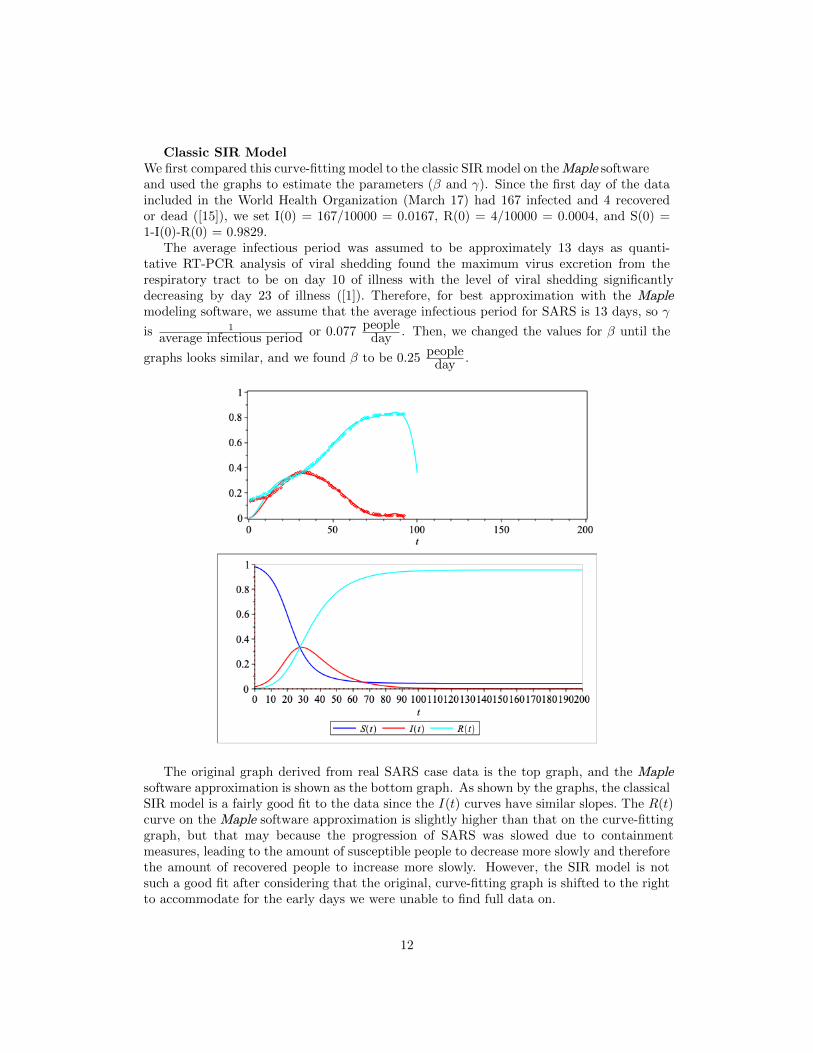
Classic SIR ModelWe first compared this curve-fitting model to the classic SIR model on the Maple softwareand used the graphs to estimate the parameters (β and γ). Since the first day of the dataincluded in the World Health Organization (March 17) had 167 infected and 4 recoveredor dead ([15]), we set I(0) = 167/10000 = 0.0167, R(0) = 4/10000 = 0.0004, and S(0) =1-I(0)-R(0) = 0.9829.

The average infectious period was assumed to be approximately 13 days as quanti-tative RT-PCR analysis of viral shedding found the maximum virus excretion from therespiratory tract to be on day 10 of illness with the level of viral shedding significantlydecreasing by day 23 of illness ([1]). Therefore, for best approximation with the Maple modeling software, we assume that the average infectious period for SARS is 13 days, so γis 1

average infectious periodor 0.077

peopleday

. Then, we changed the values for β until the

graphs looks similar, and we found β to be 0.25people

day.

The original graph derived from real SARS case data is the top graph, and the Maple software approximation is shown as the bottom graph. As shown by the graphs, the classicalSIR model is a fairly good fit to the data since the I(t) curves have similar slopes. The R(t)curve on the Maple software approximation is slightly higher than that on the curve-fittinggraph, but that may because the progression of SARS was slowed due to containmentmeasures, leading to the amount of susceptible people to decrease more slowly and thereforethe amount of recovered people to increase more slowly. However, the SIR model is notsuch a good fit after considering that the original, curve-fitting graph is shifted to the rightto accommodate for the early days we were unable to find full data on.

12

There are several limitations to the classic SIR model. First, the total population studiedand separated into the three compartments stays constant, whereas in real life, the worldpopulation is constantly changing due to births and deaths. Additionally, not every persontransfers instantaneously from one compartment to another, thus, not every infected indi-vidual becomes infectious from the onset as is assumed in the classic SIR model. There isoften a period of time, referred to as the latent infectious period where an individual is notyet infectious but has been exposed to the pathogen.

Extended SIR modelTo account for these disadvantages, we then applied the SARS case data to the extendedSIR model, which includes birth and death rates. Again, we assume that S(0) = 0.9829, I(0)= 0.0167, and R(0) = 0.0004. We also assume that the average infectious period is 13 days,

so γ is 0.077people

day. In addition, the average life expectancy for the world is 72.6 years, so

µ is 172.6 or 0.014 ([12]). By changing the values of β and trying to match the graphs, we

found β to be around 0.25people

day.

The top graph shows the case data points and fitted curves, while the bottom graph showsthe Maple approximation. The peaks for I(t) and R(t) are lower in the Maple approximationthan in the curve-fit graph, so adding birth and death rates lowered the number of infectedand recovered cases for the disease. In general, the extended SIR model was not as good asa fit as the classical SIR model. This was a rather surprising finding as one would think thatthe more specifications and variables, the more accurate the graphs would be. However, wesuspect that other factors at play, such as the µ parameter we used for life expectancy, as

13

it was the average world life expectancy, may have also lead to the dip in the I(t) and R(t)curves as compared to the real cases as the countries that were more majorly impacted bySARS tended to have higher than average life expectancies.

Even while considering more variables than the classical SIR model, there remain limi-tations to the extended SIR model. In the model, the birth rate is assumed to be equal tothe death rate, which is not true in the real world. In addition, similar to the classical SIRmodel, this model assumes that the infected people instantly become infectious upon expo-sure to an infected person, which is also untrue. This leads us to the SEIR compartmentmodel.

SEIR modelSince the SEIR model includes another compartment, the exposed group, it will likely be abetter fit for SARS since it accounts for a limitation in the first two models. One concession,though, may be that due to the difficulty of determining which fractions of population havebeen exposed to the disease but not yet infectious, there may actually be greater error inthe SEIR model than in the SIR or extended SIR models. Due to complications with datacollection and reporting, we could not obtain data for the population of individuals exposedSARS, so we were unable to create a SEIR model.

LimitationsIn the case of SARS, there is a limitation to all three nonlinear models. While the SARSoutbreak began like a classical SIR model, according to Ng et al (2003), the outbreak didnot proceed smoothly through the susceptible to infected to recovered process. ([11]) Afterbeginning in Guangzhou, SARS experienced a period of latency and background infectionwhere symptoms were little to none, after which a large outbreak appeared in Hong Kong.Because of the double-outbreak phenomenon observed with SARS, this study created theirown nonlinear compartment model they referred to as the SEIRP model, where P stands forProtected, which would account for a latency period and a maintained background infectionlevel. The normal SIR models, including the SEIR model, do not take into account thatthere may be mutations and potentially latent viruses that progress into virulent phasesat variable times, such as with SARS. Additionally, the authors of this study found thatthe parameters, even when approximated by 1% off the original values could lead to greatvariations in the total number of cases predicted by the end of the outbreak, an almostfive-fold difference, from 5000 to 116,464. Thus, the approximations we had to make mayhave led to significant errors in our calculations versus reality.

4.2 COVID-19

Nonlinear compartment models can also be applied to COVID-19. The COVID-19 pandemicstarted in Wuhan, China in December 2020, and since then, it has spread all over the globe.Currently, there are more than 2 million cases worldwide ([3]).

We gathered case data on active infected cases and total recovered and dead cases eachday from January 22, 2020 to April 21, 2020 on the COVID-19 epidemic in China, specifically([16]).

Similar to SARS, all of the 3 billion people in China cannot all be included in the totalpopulation. It would not only be impractical for modeling, but also unrealistic as Chinadid indeed forcefully close down borders in Wuhan in an attempt to contain the spread.Taking solely the population of Wuhan into consideration, there would be only 8 million

14

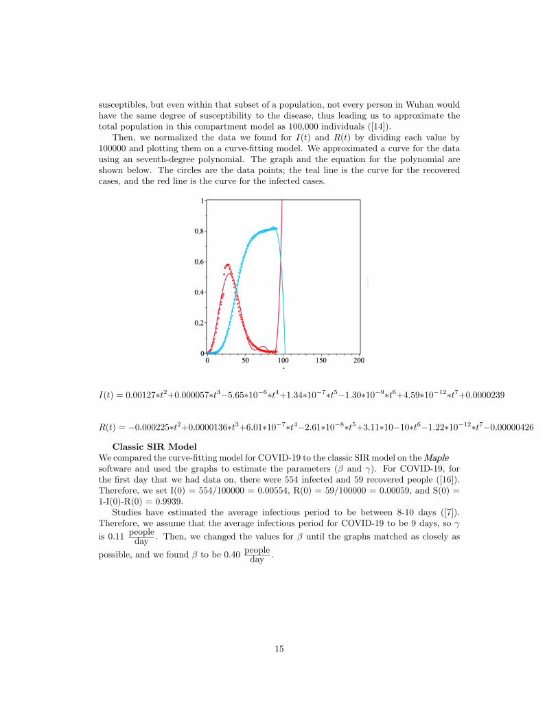
susceptibles, but even within that subset of a population, not every person in Wuhan wouldhave the same degree of susceptibility to the disease, thus leading us to approximate thetotal population in this compartment model as 100,000 individuals ([14]).

Then, we normalized the data we found for I(t) and R(t) by dividing each value by100000 and plotting them on a curve-fitting model. We approximated a curve for the datausing an seventh-degree polynomial. The graph and the equation for the polynomial areshown below. The circles are the data points; the teal line is the curve for the recoveredcases, and the red line is the curve for the infected cases.

I(t) = 0.00127∗t2+0.000057∗t3−5.65∗10−6∗t4+1.34∗10−7∗t5−1.30∗10−9∗t6+4.59∗10−12∗t7+0.0000239

R(t) = −0.000225∗t2+0.0000136∗t3+6.01∗10−7∗t4−2.61∗10−8∗t5+3.11∗10−10∗t6−1.22∗10−12∗t7−0.00000426

Classic SIR ModelWe compared the curve-fitting model for COVID-19 to the classic SIR model on the Maplesoftware and used the graphs to estimate the parameters (β and γ). For COVID-19, forthe first day that we had data on, there were 554 infected and 59 recovered people ([16]).Therefore, we set I(0) = 554/100000 = 0.00554, R(0) = 59/100000 = 0.00059, and S(0) =1-I(0)-R(0) = 0.9939.

Studies have estimated the average infectious period to be between 8-10 days ([7]).Therefore, we assume that the average infectious period for COVID-19 to be 9 days, so γis 0.11

peopleday

. Then, we changed the values for β until the graphs matched as closely as

possible, and we found β to be 0.40people

day.

15

Although the I(t) and R(t) curves are similar on both graphs, there are several differ-ences. The curve-fit real data graph has an I(t) curve that is much wider and thus spreadout over a longer period of time than the SIR model estimated I(t) curve. Additionally, theR(t) curve is much higher on the SIR model estimated curve than on the graph representingthe true recovered population growth. These results may have been the result of the limita-tions of the SIR model. First, SIR models do not take into account public health measuresenacted by governments, such as China’s strict containment policy in Wuhan, which mayhave slowed the β, or the infection transmission rate, significantly, resulting in a I(t) curvewith a lower amplitude and a longer wavelength than in the SIR model predicted graph.Furthermore, since the classical SIR model does not consider births and deaths and changesto the general studied population, it is less reflective of conditions in reality. To address thisissue, we proceed to the extended SIR model, which includes births and deaths.

Extended SIR ModelWe then compared the data for COVID-19 to the the extended SIR model, which includesbirth and death rates. Again, we assume that I(0) = 0.00554, R(0) = 0.00059, and S(0) =0.9939. We also assume that the average infectious period for COVID-19 is 9 days, so γ is

0.11people

day. The average life expectancy in China is 77.0 years ([9]), so µ is 1

77.0 or 0.0130.

We changed the values of β to match the graphs, and we found β to be 0.35people

day.

16

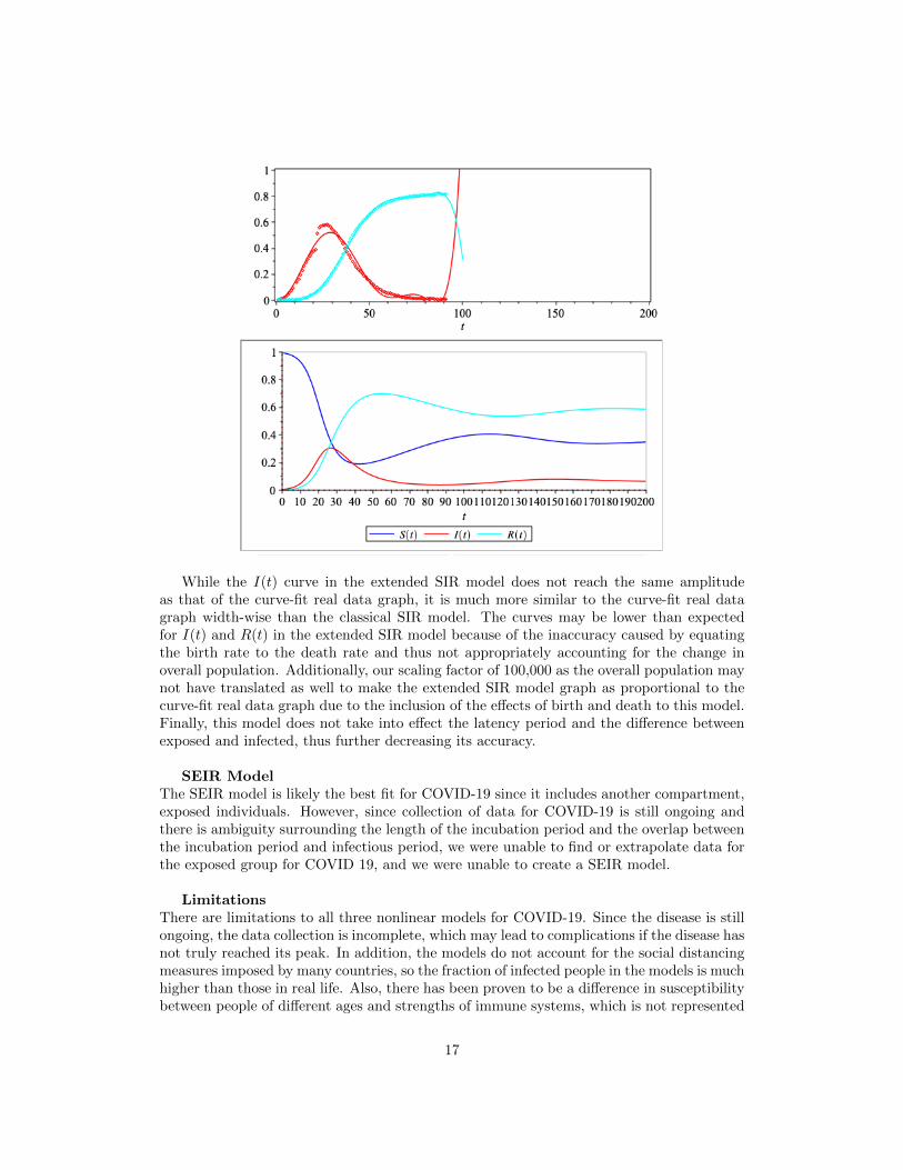
While the I(t) curve in the extended SIR model does not reach the same amplitudeas that of the curve-fit real data graph, it is much more similar to the curve-fit real datagraph width-wise than the classical SIR model. The curves may be lower than expectedfor I(t) and R(t) in the extended SIR model because of the inaccuracy caused by equatingthe birth rate to the death rate and thus not appropriately accounting for the change inoverall population. Additionally, our scaling factor of 100,000 as the overall population maynot have translated as well to make the extended SIR model graph as proportional to thecurve-fit real data graph due to the inclusion of the effects of birth and death to this model.Finally, this model does not take into effect the latency period and the difference betweenexposed and infected, thus further decreasing its accuracy.

SEIR ModelThe SEIR model is likely the best fit for COVID-19 since it includes another compartment,exposed individuals. However, since collection of data for COVID-19 is still ongoing andthere is ambiguity surrounding the length of the incubation period and the overlap betweenthe incubation period and infectious period, we were unable to find or extrapolate data forthe exposed group for COVID 19, and we were unable to create a SEIR model.

LimitationsThere are limitations to all three nonlinear models for COVID-19. Since the disease is stillongoing, the data collection is incomplete, which may lead to complications if the disease hasnot truly reached its peak. In addition, the models do not account for the social distancingmeasures imposed by many countries, so the fraction of infected people in the models is muchhigher than those in real life. Also, there has been proven to be a difference in susceptibilitybetween people of different ages and strengths of immune systems, which is not represented

17

in any of the SIR/SEIR models as they all have the same β parameter for rate of infectiontransmission.

After applying our compartment models to real infectious diseases such as SARS andCOVID-19, it appears that these models, due to their simplifications, have various limi-tations and are therefore not very accurate in modeling real infectious diseases. However,there is merit in applying these models as they are able to capture general trends, whichcan help scientists predict and better understand disease transmission in the public spherefor preparation for future and ongoing pandemics.

5 Conclusion

In this paper, we discussed the mathematics behind linear and non-linear compartment mod-els and applied such models to infectious diseases such as SARS and COVID-19. Throughour study, we have analyzed the advantages and disadvantages of each type of compartmentmodel depending on the infectious disease modeled.

Unfortunately, due to limitations in our data, we were unable to apply the SEIR modelto SARS and COVID-19. There was no data on the number of exposed people, and wewere not able to find good estimations for our parameters. We felt as if the SEIR model wewould create would be significantly inaccurate and an improper application of SEIR modelsto infectious disease. This does bring to light, however, one limitation of the SEIR model,which is the difficulty of collecting sufficiently accurate data to create the model, thus ren-dering it often impractical.

SARSOverall, out of the three nonlinear models, the SEIR model is likely the best fit for SARS,but out of the two models that we graphed, the SIR model was a better fit than the extendedSIR model. This may be because the extended SIR model assumed that the birth and deathrates were the same, and since this is not the case in the real world, it may have ended upimpacting the accuracy of the model more than the lack of births and deaths impacted theaccuracy of the classical SIR model.

COVID-19Overall, the SEIR model should theoretically be the best fit for COVID-19 due to its in-creased complexity and similarity to real-life, but out of the two models that we graphed,the extended SIR model was a better fit than the SIR model. This may be because theextended SIR model accounted for birth and death rates rather accurately in this instance,resulting in a model that better represented the data in real life.

Linear and nonlinear models exemplify the versatility and applicability of mathematicsin depicting situations in diverse fields in real life. By representing pathological, biological,and engineering processes with linear and non-linear compartment models, scientists andprofessionals can better understand their underlying mechanisms and uncover more effectiveways to combat or improve upon them.

18

19

6 References

[1] Anderson, R., et al. “Epidemiology, Transmission Dynamics and Control of SARS: The2002-2003 Epidemic.” Philosophical Transactions: Biological Sciences, vol. 359, no. 1447,2004, pp. 1091–1105. JSTOR, www.jstor.org/stable/4142242.[2] Centers for Disease Control and Prevention. Severe Acute Respiratory Syndrome.https://www.cdc.gov/sars/index.html (updated May 7, 2020)[3] Centers for Disease Control and Prevention. Coronavirus (COVID-19).https://www.cdc.gov/coronavirus/2019-ncov/index.html.(updated May 7, 2020)[4] Edenharter, G. The Classic SIR Model.https://www.maplesoft.com/applications/view.aspx?SID=153877(updated September 16, 2015)[5] Edenharter, G. The SEIR Model with Births and Deaths.https://www.maplesoft.com/applications/view.aspx?SID=153879 (updated September 16,2015)[6] Edenharter, G. The SIR Model with Births and Deaths.https://www.maplesoft.com/applications/view.aspx?SID=153878 (updated September 16,2015)[7] Housen, T., et al. How long are you infectious when you have coronavirus?https://theconversation.com/how-long-are-you-infectious-when-you-have-coronavirus-135295(updated April 12, 2020)[8] Krantz, S. G., Differential Equations. Theory, Technique, and Practice, CRC Press, USA,2015.[9] Macrotrends. China Life Expectancy 1950 - 2020. https://www.macrotrends.net/countries/CHN/china/life-expectancy[10] National Institute of Allergy and Infectious Diseases. COVID-19, MERS, SARS. https://www.niaid.nih.gov/diseases-conditions/covid-19 (updated April 6, 2020)[11] Ng, T., et al. A double epidemic model for the SARS propagation. https://www.ncbi.nlm.nih.gov/pmc/articles/PMC222908/[12] Roser, M., et al. Life Expectancy. https://ourworldindata.org/life-expectancy (updatedOctober 2019)[13] Smith, D., et al. The SIR Model for Spread of Disease - Euler’s Method for Systems.https://www.maa.org/press/periodicals/loci/joma/the-sir-model-for-spread-of-disease-eulers-method-for-systems. (updated December 2004)[14] Statista. China: population of Wuhan from 1980 to 2035. https://www.statista.com/statistics/466957/china-population-of-wuhan/. (updated May 2018)[15] World Health Organization. Cumulative Number of Reported Probable Cases of Se-vere Acute Respiratory Syndrome (SARS). https://www.who.int/csr/sars/country/en/ (up-dated 21 April 2004)[16] Worldometer. China Coronavirus. https://www.worldometers.info/coronavirus/country/china/ (updated May 7, 2020)[17] Worldometer. World Population by Year. https://www.worldometers.info/world-population/world-population-by-year/. (updated 2019)[18] Maple 2019. Maplesoft, a division of Waterloo Maple Inc. Waterloo, Ontario. Maple is atrademark of Waterloo Maple Inc.

COVID-19 Modeling

Jason Xu, Louis Li

March 2020

Abstract

COVID-19 has had a profound impact on the health, lifestyle, andeconomic well-being of the world population. The pandemic has takentens of thousands of lives and led to the greatest economic upheavalin modern history. There have been a wide array of often conflictingmodels guessing how long the crisis will last, how many people will dieor be infected, and when it will be safe to resume economic activity.Given the far-reaching economic and human impacts of governmentpolicy during this crisis, it is essential to have the most accurate datapossible. In this paper we will be using a combination of linear andnon-linear compartment models as well as multiple real world exam-ples to examine the efficacy of different models.

1 Introduction

1.1 Overview

Compartment modeling is a useful technique which can be used both to model disease infections in a population and to model drug absorption. While more complex than non-compartmental models, compartment modeling has thebenefit of being able to determine the concentration of the dependent variableat any given instant. Linear multi-compartment models are the simplest examples of compartment modeling, and rely on a population quickly transferring between ”susceptible” to ”infected” to ”recovered”. Nonlinear multi-compartment models are, by contrast, much more complex, but also a more accurate representation, taking into account the incubation period of adisease, disease-specific characteristics affecting its spread within apopulation, as well as how the number of infected people will affect the spreadof the disease.

1

1.2 Models

1.2.1 Linear

The Linear model is the most basic type of model, and only accounts forflow in one direction, in which susceptible people are infected, then recoverfrom the disease, gaining immunity. This model assumes that infected peo-ple cannot infect others, making this model suitable for situations in whichquarantines are strictly enforced, or to model drug flow through the body, asdrugs already in the body do not significantly affect the influx of new drugsinto the body.

(1.1)dS(t)

dt= −β · S(t)

(1.2)dI(t)

dt= β · S(t) − γ · I(t)

(1.3)dR(t)

dt= γ · I(t)

Figure 1: Linear Multi-Compartmental Model

1.2.2 Non-Linear

The simplest type of non-linear model is the classic SIR model, where Sstands for Susceptible, I stands for Infected, and R stands for Removed. Thismodel considers how many infected and susceptible people there are. A smallportion of susceptible or infected people will slow the spread of the diseasewith the growth rate being highest when half of the population is infectedand half is susceptible. This model will more accurately model the faster rateat which a disease spreads when more people get infected. This model alsointroduces the possibility of herd immunity in the long term because enoughpeople getting the disease will slow the rate at which the disease spreads.

(2.1)dS(t)

dt= −β · S(t) · I(t)

2

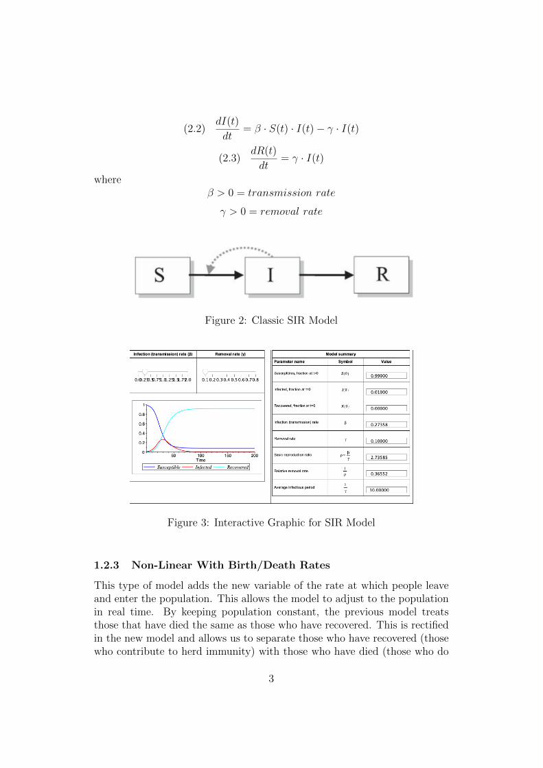
(2.2)dI(t)

dt= β · S(t) · I(t) − γ · I(t)

(2.3)dR(t)

dt= γ · I(t)

whereβ > 0 = transmission rate

γ > 0 = removal rate

Figure 2: Classic SIR Model

Figure 3: Interactive Graphic for SIR Model

1.2.3 Non-Linear With Birth/Death Rates

This type of model adds the new variable of the rate at which people leaveand enter the population. This allows the model to adjust to the populationin real time. By keeping population constant, the previous model treatsthose that have died the same as those who have recovered. This is rectifiedin the new model and allows us to separate those who have recovered (thosewho contribute to herd immunity) with those who have died (those who do

3

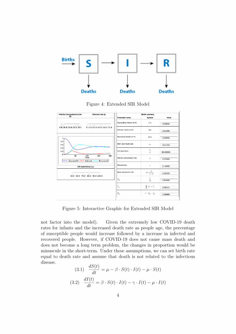
Figure 4: Extended SIR Model

Figure 5: Interactive Graphic for Extended SIR Model

not factor into the model). Given the extremely low COVID-19 deathrates for infants and the increased death rate as people age, the percentageof susceptible people would increase followed by a increase in infected andrecovered people. However, if COVID-19 does not cause mass death anddoes not become a long term problem, the changes in proportion would beminuscule in the short-term. Under these assumptions, we can set birth rateequal to death rate and assume that death is not related to the infectiousdisease.

(3.1)dS(t)

dt= µ− β · S(t) · I(t) − µ · S(t)

(3.2)dI(t)

dt= β · S(t) · I(t) − γ · I(t) − µ · I(t)

4

(3.3)dR(t)

dt= γ · I(t) − µ ·R(t)

where

µ > 0 = birth/death rate (1

µ= life expectancy)

β > 0 = transmission rate

γ > 0 = removal rate

1.2.4 Non-Linear With Exposure Rates

This type of model extends the previous models by adding yet another com-partment, representing the period in which a person is exposed (hence, E),but not yet infectious. This model can help with the often multi-week longdelays between the time a person gets infected to the time they get recordedin the data. Furthermore, given the long incubation times of many diseases,the category of ”infected” is not adequate for healthcare providers. Theymust be able to distinguish between those that need care and those thatmay need care in the future to predict the amount of resources needed atany given time. A lower exposure-to-infectious rate means that people willbecome symptomatic over a longer period of time, making it less likely thatthe medical system will be burdened at any given time.

Figure 6: SEIR Model

For COVID-19 specifically, the exposure rate could be a lot higher thancurrently reported, given the fact that exposed people are infectious, evenbefore symptoms appear. Furthermore, given the rather light severity of thedisease, many people could be exposed, but asymptomatic.

(4.1)dS(t)

dt= µ− β · S(t) · I(t) − µ · S(t)

(4.2)dE(t)

dt= β · S(t) · I(t) − σ · E(t) − µ · E(t)

5

(4.3)dI(t)

dt= σ · E − γ · I(t) − µ · I(t)

(4.4)dR(t)

dt= γ · I(t) − µ ·R(t)

where

µ > 0 = birth/death rate (1

µ= life expectancy)

β > 0 = transmission rate

σ > 0 = exposed to infectious rate

γ > 0 = removal rate

Figure 7: Interactive Graphic for SEIR Model

1.3 Basic Reproduction Ratio

If we combine all of the above variables we can get an equation for BasicReproduction Ratio. Put simply, Basic Reproduction Ratio is the expectednumber of new infections that an infectious person will produce. If this ratiois above one, then exponential growth will occur. If the ratio is below 1, then

6

the number of infected people is decreasing. Below is the Basic ReproductionRatio equation for the non-linear with exposure rates model.

ρ =β · σ

(µ+ γ) · (µ+ σ)

All of the work that has been done to mitigate the spread of COVID-19 are inthe name of reducing the output of the equation. Some factors like birthratesand exposure rates will be impossible to control during the pandemic, butdecreasing the infection rate and increasing the recovery rate will be crucialfor slowing down the rapid spread of the disease.

2 Discussion

2.1 Derivation of β and γ

To derive β and γ, we used a python script to optimize a SIR model forthe virus based on current virus data (as of 4-8-2020). The code is availableon this Github repository along with the data we used. Simply running thepython file will generate an image of the model progression, and prints thederived values of β, γ, and R0.

2.2 Derivation of Linear Differential Equations

2.2.1 Eqn. 1.1

dS(t)dt

, or the change in Susceptible, in the linear model, is simply the num-ber of people removed from the Susceptible population (ie. the number ofpeople infected) over dt. Thus, we can simply multiply the opposite of thetransmission rate (remember, people are being ”removed” from the Suscep-tible population) by the amount of currently Susceptible people , yieldingdS(t)dt

= −β · S(t), yielding equation (1.1).

2.2.2 Eqn. 1.3

dR(t)dt

is similarly simple, having only one input and no output. Therefore, wesimply multiply the rate of input (recovery rate, γ) by the amount of people

who are Infected. This yields dR(t)dt

= γ · I(t), equation (1.3).

2.2.3 Eqn. 1.2

dI(t)dt

is more complicated, having both an input and an output. Thus, wesubtract the input (new infections) from the output (recovery), derived ear-

7

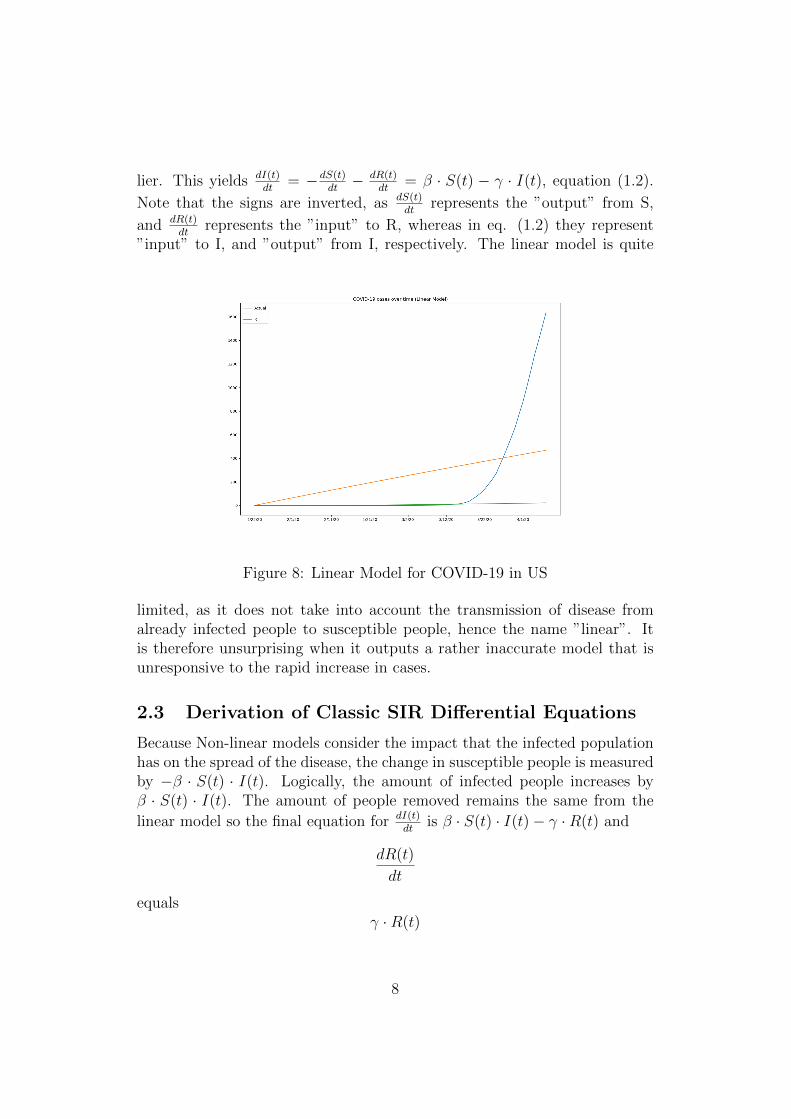
lier. This yields dI(t)dt

= −dS(t)dt

− dR(t)dt

= β · S(t) − γ · I(t), equation (1.2).

Note that the signs are inverted, as dS(t)dt

represents the ”output” from S,

and dR(t)dt

represents the ”input” to R, whereas in eq. (1.2) they represent”input” to I, and ”output” from I, respectively. The linear model is quite

Figure 8: Linear Model for COVID-19 in US

limited, as it does not take into account the transmission of disease fromalready infected people to susceptible people, hence the name ”linear”. Itis therefore unsurprising when it outputs a rather inaccurate model that isunresponsive to the rapid increase in cases.

2.3 Derivation of Classic SIR Differential Equations

Because Non-linear models consider the impact that the infected populationhas on the spread of the disease, the change in susceptible people is measuredby −β · S(t) · I(t). Logically, the amount of infected people increases byβ · S(t) · I(t). The amount of people removed remains the same from the

linear model so the final equation for dI(t)dt

is β · S(t) · I(t) − γ ·R(t) and

dR(t)

dt

equalsγ ·R(t)

8

Figure 9: Classic SIR Model for COVID-19 in US

2.4 Extended SIR Model

2.4.1 Eqn. 3.1

The extended SIR Model considers not only the effects of the disease, butalso the ”natural” birth and death rates without the disease. Thus, the Sus-ceptible population now has both an input and an output. dS(t)

dt, therefore,

must also account for the birth rate, symbolized µ. First, we must add µas, obviously, people are being added to the Susceptible population. How-ever, people are also inevitably dying off from the Susceptible population,independently of the disease. Thus, we must also subtract by µ ·S(t). Thus,dS(t)dt

= µ− β · S(t) · I(t) − µ · S(t).

2.4.2 Eqn. 3.2 and 3.3

The derivation of the extended SIR Model does not differ much from theclassic SIR Model, with respects to dI(t)

dtand dR(t)

dt, as they still have the

same inputs, and only one extra output: the deaths from each population.Thus, we must subtract µ · I(t) from dI(t)

dtand µ ·R(t) from dR(t)

dt. This yields

dI(t)dt

= β·S(t)·I(t)−γ·I(t)−µ·I(t), equation (3.2), and dR(t)dt

= γ·I(t)−µ·R(t),equation (3.3).

9

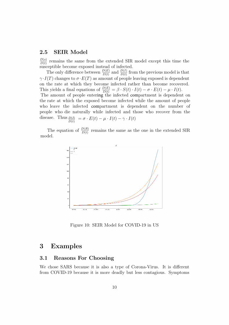
2.5 SEIR ModelD(s)D(t)

remains the same from the extended SIR model except this time thesusceptible become exposed instead of infected.

The only difference between D(E)D(t)

and D(I)D(t)

from the previous model is that

γ ·I(T ) changes to σ ·E(T ) as amount of people leaving exposed is dependenton the rate at which they become infected rather than become recovered.This yields a final equations of D(E)

D(t)= β · S(t) · I(t) − σ · E(t) − µ · I(t).

The amount of people entering the infected compartment is dependent on the rate at which the exposed become infected while the amount of peoplewho leave the infected compartment is dependent on the number of people who die naturally while infected and those who recover from thedisease. Thus D(I)

D(t)= σ · E(t) − µ · I(t) − γ · I(t)

The equation of D(R)D(t)

remains the same as the one in the extended SIRmodel.

Figure 10: SEIR Model for COVID-19 in US

3 Examples

3.1 Reasons For Choosing

We chose SARS because it is also a type of Corona-Virus. It is differentfrom COVID-19 because it is more deadly but less contagious. Symptoms

10

are usually so severe that people become hospitalized and can only infect asmall number of people.

On the other hand, Swine flu is more infectious, but less deadly thanSARS. Swine Flu’s death rate is lower than that of COVID-19, but it isestimated that 100 million were infected and 75 thousand were killed in theUnited States. Also, given the low death rate, there were no social distancingmeasures adopted. Choosing 2 diseases with higher and lower infection ratesthan COVID-19 allow us to see the effects of different infection rates.

3.2 Methodology

The code we used reads data about new infections and graphs them. Thenit will find the best values for σ, γ, β, and µ (depending on the the type ofmodel) that will create a curve that best approximates the actual data. Thebest curve is determined by root mean square regression where the valuesthat provide the lowest values for the difference in (Actual−Predicted)2 arechosen.

Linear Classic SIR SEIRCOVID-19 0.304 0.524 0.524

H1N1 0.384 0.939 0.940SARS 0.534 0.650 0.650

Table 1: r2 values for various models and diseases

As expected, the Linear model was by far the least fitting for the data.

3.3 SARS

Figure 11: Linear Model for SARS

Figure 12: Classic SIR Model for SARS

Figure 13: SEIR Model for SARS

11

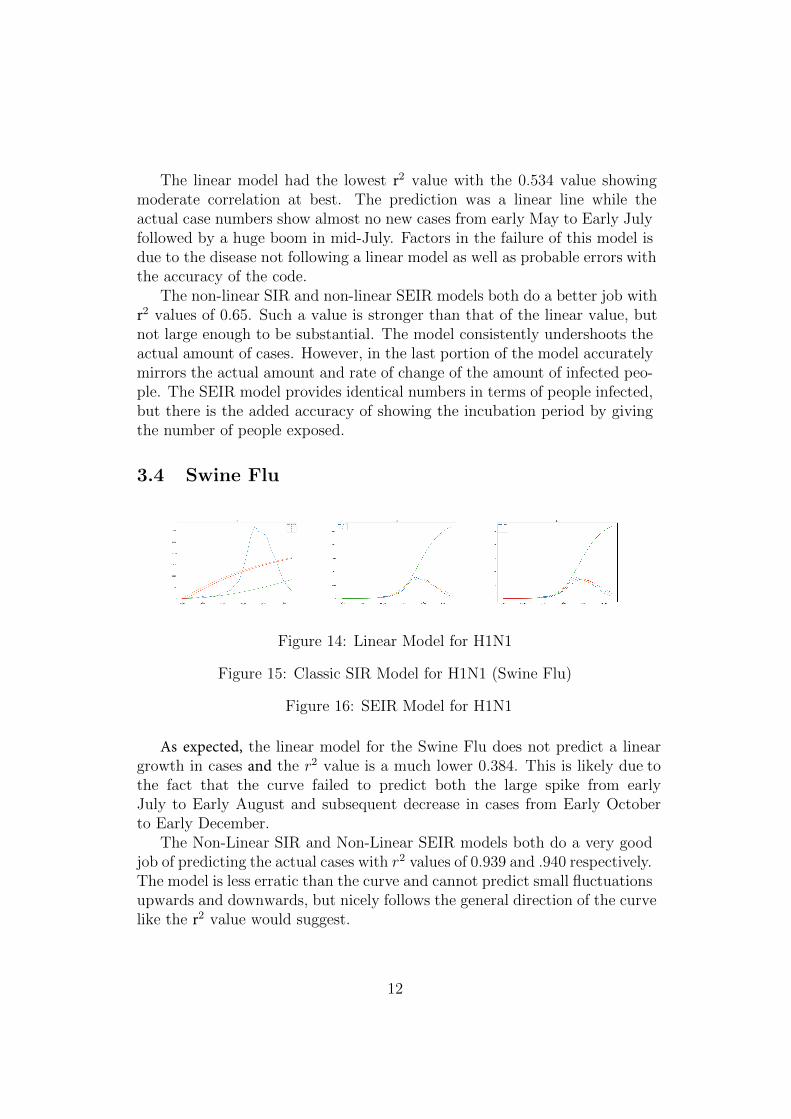
The linear model had the lowest r2 value with the 0.534 value showing moderate correlation at best. The prediction was a linear line while theactual case numbers show almost no new cases from early May to Early Julyfollowed by a huge boom in mid-July. Factors in the failure of this model isdue to the disease not following a linear model as well as probable errors withthe accuracy of the code.

The non-linear SIR and non-linear SEIR models both do a better job withr2 values of 0.65. Such a value is stronger than that of the linear value, but not large enough to be substantial. The model consistently undershoots theactual amount of cases. However, in the last portion of the model accuratelymirrors the actual amount and rate of change of the amount of infected peo-ple. The SEIR model provides identical numbers in terms of people infected,but there is the added accuracy of showing the incubation period by givingthe number of people exposed.

3.4 Swine Flu

Figure 14: Linear Model for H1N1

Figure 15: Classic SIR Model for H1N1 (Swine Flu)

Figure 16: SEIR Model for H1N1

As expected, the linear model for the Swine Flu does not predict a linear growth in cases and the r2 value is a much lower 0.384. This is likely due to the fact that the curve failed to predict both the large spike from earlyJuly to Early August and subsequent decrease in cases from Early Octoberto Early December.

The Non-Linear SIR and Non-Linear SEIR models both do a very goodjob of predicting the actual cases with r2 values of 0.939 and .940 respectively. The model is less erratic than the curve and cannot predict small fluctuationsupwards and downwards, but nicely follows the general direction of the curvelike the r2 value would suggest.

12

3.5 COVID-19

The COVID-19 linear model is the least accurate with a r2 value of 0.304. It fails to predict the large uptick in cases that began around the middle ofMarch.

The SEIR and SIR models both give r2 values of 0.524 which indicate a moderate correlation. as with the other models the amount infected initiallyovershoots the the actual cases but soon undershoots it following a largeincrease in cases starting the last week of March.

3.6 Conclusion

We will examine how each model did at predicting actual cases as well ashow the trends of each specific disease affected the accuracy of the model.

3.7 Type of Model

The linear model failed to predict the amount of cases in all instances with amedian r2 value of 0.384 due to the inaccuracies inherent to a linear model; infection rate is inherently affected by the population already infected, andso a linear model, which assumes constant rate of infection, is woefully inad-equate for modeling the spread of disease.

The SEIR and SIR models had identical median r2 values of 0.650. Both models were not completely linear and better followed the general increasein actual cases. However, neither model was good at predicting a decrease incases or a rapid increase. Given that these models take into account the factthat a larger infected population will lead to a faster growth in infections inthe short-term, it makes sense that they are more accurate than the linearmodel.

3.8 Specific Disease

For this section the r2 values for SEIR and SIR will be treated as one value in the calculation of the mean given that they are practically identical for all3 diseases.

SARS had the smallest difference in r2 value between linear and non-linear models with only a 0.116 difference. The actual amount of cases constantlyincreased at the beginning, but at a relatively slow rate. This was followed bya rapid increase starting in the middle of July. The models

13

accurately predicted the actual cases towards the end of the time period, butnot at the start.

For H1N1 the difference of 0.636 between the r2 values was by far the largest of all 3 diseases. The change in cases for H1N1 was much less erraticthan the other diseases as it did not feature a large spike in cases like SARS orhave incomplete data like COVID 19.

Primarily due to the nature of H1N1, it was better predicted than COVID and SARS, but was also partially due to our computer program and the lack of large changes in cases for H 1N1. O ur program does curve fitting by selectingvalues for σ, γ, β, and µ that would create the least value for residuals squared.This methodology m eans that every change will affect the entirety of the m odelrather than a portion. This is fine if there are no rapid changes as in H1N1, butif there is a quick increase or quick decrease as in SARS, then the model has toincrease the number of cases early on to stay close to the larger number ofcases later on. This compounded with the fact that root mean squaretakes into account a few large residuals much more than a large amount ofsmall residuals means that our model often begins by overshooting and thenundershoots.

References

[1] Derek Hawkins, M. B. Trump declares Coronavirus outbreak a na-

tional emergency https://www.washingtonpost.com/world/2020/03/13/coronavirus-latest-news/ (accessed Apr 9, 2020).

[2] Department of Communicable Disease Surveillance and Response, Con-sensus document on the epidemiology of severe acute respiratory syn-drome (SARS). World Health Organization 2003, 7–8.

[3] Helen Branswell, H. B.; Branswell, H.; H, C.; Muchacos, J.; Hithere;Kerry; Russell, J.; Machi, A.; Brian; Carol The last flu pandemic was a’quiet killer.’ Why we can’t predict the next one https://www.statnews.com/2019/06/11/h1n1-swine-flu-10-years-later/.

[4] Jilani, T. N.; Jamil, R. T.; Siddiqi, A. H. H1N1 Influenza (Swine Flu).NCBI 2019.

[5] Sasaki, Kai COVID-19 SIR model estimation https://github.com/Lewuathe/COVID19-SIR

14

[6] JHU CCSE COVID-19 Data Repository https://github.com/CSSEGISandData/COVID-19