Yuktibhasa the First Textbook of Calculus Yuktibhas Kerala School

CALCULUSEarly Transcendentals
Integral & Multi-Variable
Calculus for Social Sciences
LICENSE
Creative Commons License (CC BY-NC-SA)
This text, including the art and illustrations, are available under the Creative Commons license (CC BY-
NC-SA), allowing anyone to reuse, revise, remix and redistribute the text. For more info visit
http://creativecommons.org/licenses/bync-sa/4.0/
Calculus Early Transcendentals Integral & Multi-Variable Calculus for Social Sciences was adapted
by Petra Menz and Nicola Mulberry from Lyryx’ textbook, Calculus Early Transcendentals an Open
Text (VERSION 2017- REVISION A) licensed under a Creative Commons Attribution Non-Commercial
Share-Alike 3.0 Unported License (CC BY-NC-SA 3.0). For information about what was changed in this
adaptation, refer to the Copyright statement on the next page.

iii
Unless otherwise noted, Calculus Early Transcendentals for Integral & Multi-Variable Calculus for Social
Sciences is (c) 2018 by Lyryx. The textbook content was produced by Lyryx Learning Team and is licensed
under a Creative Commons Attribution Non-commercial Share-Alike 3.0 Unported license, except for the
following changes and additions, which are (c) 2018 by Petra Menz, and are licensed under a Creative
Commons Attribution Non-commercial Share-Alike 4.0 International license. Examples, in particular
applications, have been added throughout the textbook to further illustrate concepts and to reflect social
science calculus content; exercises have been added throughout the textbook to provide more extensive
practice, and information throughout the book, as applicable, has been revised to reflect social science
calculus content and modified to visually align definitions, theorems and guidelines established in the
textbook.
The following additions have been made to these chapters:
Chapter 1:
◮ Antiderivatives
Chapter 2:
◮ Partial Fraction Method
Chapter 3:
◮ Business and Economics Applications
Chapter 4:
◮ Probability: One Random Variable, Two Random Variables
Chapter 5:
◮ Classifying Differential Equations
◮ Simple Growth and Decay Model, Logistic Growth Model
◮ Slope Fields
The following deletions have been made: Review, Functions, Limits, Derivatives, Applications of Deriva-
tives, Selected Applications of Integration (Distance, Velocity, Acceleration, Work, Centre of Mass, Arc
Length, Surface Area), Polar Coordinates, Parametric Equations, Three Dimensions, Partial Differentia-
tion, Vector Functions, and Vector Calculus.

iv
Acknowledgements
The production of this textbook and supplementary material was made possible under an SFU Open Edu-
cational Resources Grant and matching funds from the Department of Mathematics. The authors acknowl-
edge the helpful advice received from the following staff at SFU:
Hope Power, Teaching & Learning Librarian, SFU
Jennifer Zerkee, Copyright Specialist, SFU Copyright Office
Cindy Xin, Educational Consultant, SFU Teaching and Learning Centre.
We are indebted to John Stockie for his careful proofreading of the text, but moreover, for providing
constructive criticism that further helped shape the adaption into a cohesive student-oriented calculus text.
OER Support: Corrections and Suggestions
Please support OER. In an effort to improve the content of this textbook, contact Petra Menz at [email protected]
with your suggestions for improvements, new content, or errata.
Dedication
To my son Eli, so that his access to learning remains open as he unfolds his wings to explore life. May his
roots be strong and anchor him in all of his pursuits.
Petra Menz
Contents
Contents v
Introduction 1
Problem Solving Strategies 2
1 Integration 3
1.1 Antiderivatives . . . . . . . . . . . . . . . . . . . . . . . . . . . . . . . . . . . . . . . . 3
1.2 Displacement and Area . . . . . . . . . . . . . . . . . . . . . . . . . . . . . . . . . . . . 4
1.3 Riemann Sums . . . . . . . . . . . . . . . . . . . . . . . . . . . . . . . . . . . . . . . . 7
1.4 The Definite Integral and FTC . . . . . . . . . . . . . . . . . . . . . . . . . . . . . . . . 23
1.4.1 Exploring an Example . . . . . . . . . . . . . . . . . . . . . . . . . . . . . . . . 23
1.4.2 Defining the Definite Integral . . . . . . . . . . . . . . . . . . . . . . . . . . . . 24
1.4.3 The Fundamental Theorem of Calculus . . . . . . . . . . . . . . . . . . . . . . . 27
1.4.4 Notation when Computing a Definite Integral . . . . . . . . . . . . . . . . . . . . 30
1.4.5 Computing a Definite Integral . . . . . . . . . . . . . . . . . . . . . . . . . . . . 31
1.5 Indefinite Integrals . . . . . . . . . . . . . . . . . . . . . . . . . . . . . . . . . . . . . . 37
1.5.1 Defining the Indefinite Integral . . . . . . . . . . . . . . . . . . . . . . . . . . . . 37
1.5.2 Definite Integral versus Indefinite Integral . . . . . . . . . . . . . . . . . . . . . . 39
1.5.3 Computing Indefinite Integrals . . . . . . . . . . . . . . . . . . . . . . . . . . . . 40
1.5.4 Differential Equations and Constants of Integration . . . . . . . . . . . . . . . . . 44
2 Techniques of Integration 48
2.1 Substitution Rule . . . . . . . . . . . . . . . . . . . . . . . . . . . . . . . . . . . . . . . 48
2.1.1 Substitution Rule for Indefinite Integrals . . . . . . . . . . . . . . . . . . . . . . . 48
2.1.2 Substitution Rule for Definite Integrals . . . . . . . . . . . . . . . . . . . . . . . 55
2.2 Powers of Trigonometric Functions . . . . . . . . . . . . . . . . . . . . . . . . . . . . . . 58
2.2.1 Products of Powers of Sine and Cosine . . . . . . . . . . . . . . . . . . . . . . . 58
2.2.2 Exploring Powers of Secant and Tangent . . . . . . . . . . . . . . . . . . . . . . 63
2.2.3 Products of Powers of Secant and Tangent . . . . . . . . . . . . . . . . . . . . . . 65
2.3 Trigonometric Substitutions . . . . . . . . . . . . . . . . . . . . . . . . . . . . . . . . . 68
2.4 Integration by Parts . . . . . . . . . . . . . . . . . . . . . . . . . . . . . . . . . . . . . . 75
2.4.1 The Tabular Method . . . . . . . . . . . . . . . . . . . . . . . . . . . . . . . . . 78
2.5 Partial Fraction Method for Rational Functions . . . . . . . . . . . . . . . . . . . . . . . 80
v

vi Contents
2.5.1 Using Substitution Rule with Rational Fractions . . . . . . . . . . . . . . . . . . 80
2.5.2 Denominator with Distinct Linear Factors . . . . . . . . . . . . . . . . . . . . . . 81
2.5.3 Denominator with Irreducible Quadratic Factor . . . . . . . . . . . . . . . . . . . 86
2.5.4 Summary . . . . . . . . . . . . . . . . . . . . . . . . . . . . . . . . . . . . . . . 87
2.6 Numerical Integration . . . . . . . . . . . . . . . . . . . . . . . . . . . . . . . . . . . . . 88
2.6.1 The Midpoint Rule . . . . . . . . . . . . . . . . . . . . . . . . . . . . . . . . . . 88
2.6.2 The Trapezoid Rule . . . . . . . . . . . . . . . . . . . . . . . . . . . . . . . . . . 89
2.6.3 Simpson’s Rule . . . . . . . . . . . . . . . . . . . . . . . . . . . . . . . . . . . . 92
2.7 Improper Integrals . . . . . . . . . . . . . . . . . . . . . . . . . . . . . . . . . . . . . . 95
2.7.1 Improper Integrals: Infinite Limits of Integration . . . . . . . . . . . . . . . . . . 97
2.7.2 Improper Integrals: Discontinuities . . . . . . . . . . . . . . . . . . . . . . . . . 99
2.7.3 p-Integrals . . . . . . . . . . . . . . . . . . . . . . . . . . . . . . . . . . . . . . 102
2.7.4 The Comparison Test . . . . . . . . . . . . . . . . . . . . . . . . . . . . . . . . . 104
2.8 Additional exercises . . . . . . . . . . . . . . . . . . . . . . . . . . . . . . . . . . . . . . 106
3 Applications of Integration 108
3.1 Average Value and Area Revisited . . . . . . . . . . . . . . . . . . . . . . . . . . . . . . 108
3.1.1 Average Value of a Function . . . . . . . . . . . . . . . . . . . . . . . . . . . . . 108
3.1.2 Area of Symmetric Functions . . . . . . . . . . . . . . . . . . . . . . . . . . . . 110
3.1.3 Area Between Curves: Integration w.r.t x . . . . . . . . . . . . . . . . . . . . . . 112
3.1.4 Area Between Curves: Integration w.r.t. y . . . . . . . . . . . . . . . . . . . . . . 118
3.2 Applications to Business and Economics . . . . . . . . . . . . . . . . . . . . . . . . . . . 122
3.2.1 Surplus in Consumption and Production . . . . . . . . . . . . . . . . . . . . . . . 122
3.2.2 Continuous Money Flow . . . . . . . . . . . . . . . . . . . . . . . . . . . . . . . 128
3.3 Volume of Revolution: Disk Method . . . . . . . . . . . . . . . . . . . . . . . . . . . . . 136
3.3.1 Computing Volumes with Cross-sections . . . . . . . . . . . . . . . . . . . . . . 136
3.3.2 Disk Method: Integration w.r.t. x . . . . . . . . . . . . . . . . . . . . . . . . . . . 140
3.3.3 Washer Method: Integration w.r.t x . . . . . . . . . . . . . . . . . . . . . . . . . . 143
3.3.4 Disk and Washer Methods: Integration w.r.t. y . . . . . . . . . . . . . . . . . . . . 147
3.3.5 Summary . . . . . . . . . . . . . . . . . . . . . . . . . . . . . . . . . . . . . . . 150
3.4 Volume of Revolution: Shell Method . . . . . . . . . . . . . . . . . . . . . . . . . . . . . 154
3.4.1 Shell Method: Integration w.r.t. x . . . . . . . . . . . . . . . . . . . . . . . . . . 155
3.4.2 Shell Method: Integration w.r.t. y . . . . . . . . . . . . . . . . . . . . . . . . . . 161
3.4.3 Summary . . . . . . . . . . . . . . . . . . . . . . . . . . . . . . . . . . . . . . . 164
4 Multiple Integration 168
4.1 Functions of Several Variables . . . . . . . . . . . . . . . . . . . . . . . . . . . . . . . . 168
4.2 Double Integrals: Volume and Average Value . . . . . . . . . . . . . . . . . . . . . . . . 178
4.2.1 Volume and Average Value over a Rectangular Region . . . . . . . . . . . . . . . 178
Contents vii
4.2.2 Computing Double Integrals over Rectangular Regions . . . . . . . . . . . . . . . 180
4.2.3 Computing Double Integrals over any Region . . . . . . . . . . . . . . . . . . . . 184
4.3 Triple Integrals: Volume and Average Value . . . . . . . . . . . . . . . . . . . . . . . . . 188
4.4 Probability . . . . . . . . . . . . . . . . . . . . . . . . . . . . . . . . . . . . . . . . . . . 194
4.4.1 One Random Variable . . . . . . . . . . . . . . . . . . . . . . . . . . . . . . . . 194
4.4.1.1 Discrete Example . . . . . . . . . . . . . . . . . . . . . . . . . . . . . 194
4.4.1.2 Discrete and Continuous Random Variables . . . . . . . . . . . . . . . 195
4.4.1.3 Probability Density and Cumulative Distribution . . . . . . . . . . . . . 196
4.4.1.4 Expected Value, Variance and Standard Deviation . . . . . . . . . . . . 202
4.4.1.5 Normal Distribution . . . . . . . . . . . . . . . . . . . . . . . . . . . . 209
4.4.2 Two Random Variables . . . . . . . . . . . . . . . . . . . . . . . . . . . . . . . . 212
4.4.2.1 Joint Probability Density and Joint Cumulative Distribution . . . . . . . 212
4.4.2.2 Expected Value, Variance and Covariance . . . . . . . . . . . . . . . . 217
5 Differential Equations 225
5.1 Classifying Differential Equations . . . . . . . . . . . . . . . . . . . . . . . . . . . . . . 226
5.2 First Order Differential Equations . . . . . . . . . . . . . . . . . . . . . . . . . . . . . . 229
5.2.1 Initial Value Problems . . . . . . . . . . . . . . . . . . . . . . . . . . . . . . . . 230
5.2.2 Separable Equations . . . . . . . . . . . . . . . . . . . . . . . . . . . . . . . . . 233
5.2.3 Simple Growth and Decay Model . . . . . . . . . . . . . . . . . . . . . . . . . . 235
5.2.4 Logistic Growth Model . . . . . . . . . . . . . . . . . . . . . . . . . . . . . . . . 238
5.3 First Order Linear Differential Equations . . . . . . . . . . . . . . . . . . . . . . . . . . . 242
5.3.1 Homogeneous DEs . . . . . . . . . . . . . . . . . . . . . . . . . . . . . . . . . . 242
5.3.2 Non-Homogeneous DEs . . . . . . . . . . . . . . . . . . . . . . . . . . . . . . . 243
5.4 Approximation . . . . . . . . . . . . . . . . . . . . . . . . . . . . . . . . . . . . . . . . 250
5.4.1 Slope Field . . . . . . . . . . . . . . . . . . . . . . . . . . . . . . . . . . . . . . 250
5.4.2 Euler’s Method . . . . . . . . . . . . . . . . . . . . . . . . . . . . . . . . . . . . 257
6 Sequences and Series 265
6.1 Sequences . . . . . . . . . . . . . . . . . . . . . . . . . . . . . . . . . . . . . . . . . . . 266
6.2 Series . . . . . . . . . . . . . . . . . . . . . . . . . . . . . . . . . . . . . . . . . . . . . 275
6.3 The Integral Test . . . . . . . . . . . . . . . . . . . . . . . . . . . . . . . . . . . . . . . 281
6.4 Alternating Series . . . . . . . . . . . . . . . . . . . . . . . . . . . . . . . . . . . . . . . 287
6.5 Comparison Test . . . . . . . . . . . . . . . . . . . . . . . . . . . . . . . . . . . . . . . 290
6.6 Absolute and Conditional Convergence . . . . . . . . . . . . . . . . . . . . . . . . . . . 293
6.7 The Ratio and Root Tests . . . . . . . . . . . . . . . . . . . . . . . . . . . . . . . . . . . 296
6.8 Power Series and Polynomial Approximation . . . . . . . . . . . . . . . . . . . . . . . . 299
6.8.1 Power Series . . . . . . . . . . . . . . . . . . . . . . . . . . . . . . . . . . . . . 299
6.8.2 Calculus with Power Series . . . . . . . . . . . . . . . . . . . . . . . . . . . . . 305

viii Contents
6.8.3 Maclaurin Series and Taylor Series . . . . . . . . . . . . . . . . . . . . . . . . . 307
6.8.4 Taylor Polynomials . . . . . . . . . . . . . . . . . . . . . . . . . . . . . . . . . . 313
6.8.5 Taylor’s Theorem . . . . . . . . . . . . . . . . . . . . . . . . . . . . . . . . . . . 316
Selected Exercise Answers 323
Index 342

Introduction
This course is designed for students specializing in business or the social sciences. Topics include in-
tegration; a variety of techniques of integration; applications of integration such as average value, area,
volume using Disk and Shell Methods, surplus in consumption and production, continuous money flow,
double and triple integration, and probability; differential equations; and sequences and series leading up
to Taylor’s Theorem.
The following Recommendations for Success in Mathematics are excerpts taken from the same named
document published by Petra Menz in order to provide strategies grouped into categories to all students
who are thinking about their well-being, learning, and goals, and who want to be successful academically.
How to Take Lecture Notes:
Listen to the Instructor, who
◮ explains the concepts;
◮ draws connections;
◮ demonstrates examples;
◮ emphasizes material.
Copy the presented lecture material
◮ by arriving to the lecture prepared;
◮ using telegraphic writing, i.e. packing as much information into the smallest possible number of
words/ symbols (do you really need to copy all the algebraic/manipulative steps?).
Mark up your notes immediately while listening and copying using a system such as offered here:
! pay attention (possible exam material)
? confusing (read course notes or visit ACW )
-> practice (using course notes and online assignments)
underline/highlight key concepts
Habits of a Successful Student: for detailed description of each item see the document Recommendations
for Success in Mathematics
◮ Acts responsibly
◮ Sets goals
◮ Is reflective
◮ Is inquisitive
◮ Can communicate
◮ Enjoys learning
◮ Is resourceful
◮ Is organized
◮ Manages time effectively
◮ Is involved
1

Problem Solving Strategies
The emphasis in this course is on problems–doing calculations and applications. To master problem
solving one needs a tremendous amount of practice doing problems. The more problems you do the
better you will be at doing them, as patterns will start to emerge in both the problems and in successful
approaches to them. You will learn quickly and effectively if you devote some time to doing problems
every day.
Typically the most difficult problems are applications, since they require some effort before you can begin
calculating. Here are some pointers for doing applications:
1. Carefully read each problem twice before writing anything.
2. Assign letters to quantities that are described only in words; draw a diagram if appropriate.
3. Decide which letters are constants (invariants) and which are variables (variants). A letter stands for
a constant if its value remains the same throughout the problem. A letter stands for a variable if its
value varies throughout the problem.
4. Using mathematical notation, write down what you know and then write down what you want to
find.
5. Decide what category of problem it is (this might be obvious if the problem comes at the end of a
particular chapter, but will not necessarily be so obvious if it comes on an exam covering several
chapters).
6. Double check each step as you go along; don’t wait until the end to check your work.
7. Use common sense; if an answer is out of the range of practical possibilities, then check your work
to see where you went wrong
2

1. Integration
1.1 Antiderivatives
You have probably taken a course in Differential Calculus, where you have solved problems of the follow-
ing nature:
• Given f (x) = sin(x)+3x5 −12, find f ′(x).
• Given the position function of an object, determine its velocity function.
• Given the demand function, calculate the elasticity of demand.
To solve any of these problems we need the concept of the derivative, which provides us with information
about the rate of change of the quantity involved that leads to the solution. In other words, Differential
Calculus allows us to solve problems that are concerned with finding the rate of change of one quantity
with respect to another quantity.
The next three chapters are based on the idea of the antiderivative, which basically helps us solve
problems that are the reverse of the above problems such as
• Given f ′(x) = sin(x)+3x5 −12, find f (x).
• Given the velocity function of an object, determine its position function.
• How much do consumers benefit by purchasing some manufactured goods at the price determined
by supply and demand?
We will develop tools for finding the antiderivative, which is the process of antidifferentiation also known
as integration. Hence, these kinds of problems fall under the topic of Integral Calculus. In summary, In-
tegral Calculus allows us to solve problems, where the rate of change of one quantity is given with respect
to another quantity and we are concerned with finding the relationship between these two quantities.
Definition 1.1: Antiderivative
A function F is an antiderivative of f on an interval I if
F ′(x) = f (x)
for all x in I.
3

4 Integration
1.2 Displacement and Area
We will now delve into two examples, one concerning displacement and the other area, to explore how the
antidifferentiation process should unfold.
Example 1.2: Object Moving in a Straight Line
An object moves in a straight line so that its speed at time t is given by v(t) = 3t in, say, cm/sec. If
the object is at position 10 on the straight line when t = 0, where is the object at any time t?
Solution. There are two reasonable ways to approach this problem.
Method 1: If s(t) is the position of the object at time t, we know that s′(t) = v(t). Based on our knowledge
of derivatives, we therefore know that
s(t) = 3t2/2+ k,
and because s(0) = 10 we easily discover that k = 10, so
s(t) = 3t2/2+10.
For example, at t = 1 the object is at position 3/2+10 = 11.5 cm.
This is certainly the easiest way to deal with this problem. Not all similar problems are so easy, as we
will see; the second approach to the problem is more difficult but also more general.
Method 2: We start by considering how we might approximate a solution. We know that at t = 0 the
object is at position 10. How might we approximate its position at, say, t = 1? We know that the speed of
the object at time t = 0 is 0; if its speed were constant then in the first second the object would not move
and its position would still be 10 when t = 1. In fact, the object will not be too far from 10 at t = 1, but
certainly we can do better.
Let’s look at the times 0.1, 0.2, 0.3, . . . , 1.0, and try approximating the location of the object at each,
by supposing that during each tenth of a second the object is going at a constant speed. Since the object
initially has speed 0, we again suppose it maintains this speed, but only for a tenth of second; during that
time the object would not move. During the tenth of a second from t = 0.1 to t = 0.2, we suppose that the
object is travelling at 0.3 cm/sec, namely, its actual speed at t = 0.1. In this case the object would travel
(0.3)(0.1) = 0.03 centimetres: 0.3 cm/sec times 0.1 seconds. Similarly, between t = 0.2 and t = 0.3 the
object would travel (0.6)(0.1) = 0.06 centimetres. Continuing, we get as an approximation that the object
travels
(0.0)(0.1)+(0.3)(0.1)+(0.6)(0.1)+ · · ·+(2.7)(0.1) = 1.35
centimetres, ending up at position 11.35 cm. This is a better approximation than 10, certainly, but is still
just an approximation. (We know in fact that the object ends up at position 11.5, because we’ve already
done the problem using the first approach.)
Presumably, we will get a better approximation if we divide the time into one hundred intervals of a
hundredth of a second each, and repeat the process:
(0.0)(0.01)+(0.03)(0.01)+(0.06)(0.01)+ · · ·+(2.97)(0.01) = 1.485.
We thus approximate the position as 11.485. Since we know the exact answer, we can see that this is much
closer, but if we did not already know the answer, we wouldn’t really know how close.

1.2. Displacement and Area 5
We can keep this up, but we’ll never really know the exact answer if we simply compute more and
more examples. Let’s instead look at a “typical” approximation. Suppose we divide the time into n equal
intervals, and imagine that on each of these the object travels at a constant speed. Over the first time inter-
val we approximate the distance travelled as (0.0)(1/n) = 0, as before. During the second time interval,
from t = 1/n to t = 2/n, the object travels approximately 3(1/n)(1/n) = 3/n2 centimetres. During time
interval number i, the object travels approximately (3(i− 1)/n)(1/n) = 3(i− 1)/n2 centimetres, that is,
its speed at time (i−1)/n, 3(i−1)/n, times the length of time interval number i, 1/n. Adding these up as
before, we approximate the distance travelled as
(0)1
n+3
1
n2+3(2)
1
n2+3(3)
1
n2+ · · ·+3(n−1)
1
n2
centimetres. What can we say about this? At first it looks rather less useful than the concrete calculations
we’ve already done, but in fact a bit of algebra reveals it to be much more useful. We can factor out a 3
and 1/n2 to get3
n2(0+1+2+3+ · · ·+(n−1)),
that is, 3/n2 times the sum of the first n−1 positive integers.
Now we make use of a fact you may have run across before, Gauss’s Equation:
1+2+3+ · · ·+ k =k(k+1)
2.
In our case we’re interested in k = n−1, so
1+2+3+ · · ·+(n−1) =(n−1)(n)
2=
n2 −n
2.
This simplifies the approximate distance travelled to
3
n2
n2 −n
2=
3
2
n2 −n
n2=
3
2
(
n2
n2− n
n2
)
=3
2
(
1− 1
n
)
.
Now this is quite easy to understand: as n gets larger and larger this approximation gets closer and closer
to (3/2)(1−0) = 3/2, so that 3/2 is the exact distance traveled during one second, and the final position
is 11.5.
So for t = 1, at least, this rather cumbersome approach gives the same answer as the first approach. But
really there’s nothing special about t = 1; let’s just call it t instead. In this case the approximate distance
traveled during time interval number i is 3(i− 1)(t/n)(t/n) = 3(i− 1)t2/n2, that is, speed 3(i− 1)(t/n)times time t/n, and the total distance traveled is approximately
(0)t
n+3(1)
t2
n2+3(2)
t2
n2+3(3)
t2
n2+ · · ·+3(n−1)
t2
n2.
As before we can simplify this to
3t2
n2(0+1+2+ · · ·+(n−1)) =
3t2
n2
n2 −n
2=
3
2t2
(
1− 1
n
)
.

6 Integration
In the limit, as n gets larger, this gets closer and closer to (3/2)t2 and the approximated position of the
object gets closer and closer to (3/2)t2 + 10, so the actual position is (3/2)t2 + 10, exactly the answer
given by the first method to the problem.
♣
Example 1.3: Area under the Line
Find the area under the curve y = 3x between x = 0 and any positive value x = a.
Solution. There is here no obvious analogue to the first method in the previous example, but the second
method works fine. (Since the function y = 3x is so simple, there is another method that works here, but it
is even more limited in potential application than is method number one.) How might we approximate the
desired area? We know how to compute areas of rectangles, so we approximate the area by rectangles as
shown below.
y = 3x
. . .
an
(n−1)an
a
3(n−1)an
x
y
Jumping straight to the general case, suppose we divide the interval between 0 and a into n equal
subintervals, and use a rectangle above each subinterval to approximate the area under the curve. There
are many ways we might do this, but let’s use the height of the curve at the left endpoint of the subinterval
as the height of the rectangle. The height of rectangle number i is then 3(i−1)(a/n), the width is a/n, and
the area is 3(i−1)(a2/n2). The total area of the rectangles is
(0)a
n+3(1)
a2
n2+3(2)
a2
n2+3(3)
a2
n2+ · · ·+3(n−1)
a2
n2.
By factoring out 3a2/n2 this simplifies to
3a2
n2(0+1+2+ · · ·+(n−1)) =
3a2
n2
n2 −n
2=
3
2a2
(
1− 1
n
)
.
As n gets larger this gets closer and closer to 3a2/2, which must therefore be the true area under the curve.
♣

1.3. Riemann Sums 7
What you will have noticed, of course, is that while the problem in the second example appears to
be much different than the problem in the first example, and while the easy approach to problem one
does not appear to apply to problem two, the “approximation” approach works in both, and moreover the
calculations are identical. As we will see, there are many, many problems that appear much different on
the surface but turn out to be the same as these problems, in the sense that when we try to approximate
solutions we end up with mathematics that looks like the two examples, though of course the function
involved will not always be so simple.
Even better, we now see that while the second problem did not appear to be amenable to approach one,
it can in fact be solved in the same way. The reasoning is this: we know that problem one can be solved
easily by finding a function whose derivative is 3t. We also know that mathematically the two problems
are the same, because both can be solved by taking a limit of a sum, and the sums are identical. Therefore,
we don’t really need to compute the limit of either sum because we know that we will get the same answer
by computing a function with the derivative 3t or, which is the same thing, 3x.
It’s true that the first problem had the added complication of the “10”, and we certainly need to be able
to deal with such minor variations, but that turns out to be quite simple. The lesson then is this: whenever
we can solve a problem by taking the limit of a sum of a certain form, instead of computing the (often
nasty) limit we can find a new function with a certain derivative.
Exercises for Section 1.2
Exercise 1.2.1 Suppose an object moves in a straight line so that its speed at time t is given by v(t) =2t +2, and that at t = 1 the object is at position 5. Find the position of the object at t = 2.
Exercise 1.2.2 Suppose an object moves in a straight line so that its speed at time t is given by v(t)= t2+2,
and that at t = 0 the object is at position 5. Find the position of the object at t = 2.
1.3 Riemann Sums
A fundamental calculus technique is to first answer a given problem with an approximation, then refine
that approximation to make it better, then use limits in the refining process to find the exact answer. That
is exactly what we will do here to develop a technique to find the area of more complicated regions.
Consider the region given in Figure 1.1, which is the area under y = 4x− x2 on [0,4]. What is the
signed area of this region when the area above the x-axis is positive and below negative?

8 Integration
1 2 3 4
1
2
3
4
x
y
Figure 1.1: f (x) = 4x− x2
We start by approximating. We can surround the region with a rectangle with height and width of
4 and find the area is approximately 16 square units. This is obviously an over–approximation; we are
including area in the rectangle that is not under the parabola. How can we refine our approximation to
make it better? The key to this section is this answer: use more rectangles.
Let’s use four rectangles of equal width of 1. This partitions the interval [0,4] into four subintervals,
[0,1], [1,2], [2,3] and [3,4]. On each subinterval we will draw a rectangle.
There are three common ways to determine the height of these rectangles: the Left Hand Rule, the
Right Hand Rule, and the Midpoint Rule:
• The Left Hand Rule says to evaluate the function at the left-hand endpoint of the subinterval and
make the rectangle that height. In Figure 1.2, the rectangle labelled “LHR” is drawn on the interval
[2,3] with a height determined by the Left Hand Rule, namely f (2) = 4.
• The Right Hand Rule says the opposite: on each subinterval, evaluate the function at the right
endpoint and make the rectangle that height. In Figure 1.2, the rectangle labelled “RHR” is drawn
on the interval [0,1] with a height determined by the Right Hand Rule, namely f (1) = 3.
• The Midpoint Rule says that on each subinterval, evaluate the function at the midpoint and make
the rectangle that height. In Figure 1.2, the rectangle labelled “MPR” is drawn on the interval [1,2]with a height determined by the Midpoint Rule, namely f (1.5) = 3.75.
• These are the three most common rules for determining the heights of approximating rectangles, but
we are not forced to use one of these three methods. In Figure 1.2, the rectangle labelled “other” is
drawn on the interval [3,4] with a height determined by choosing a random x-value on the interval
[3,4]. The chosen x-value is 3.54, which yields a height of f (3.54).

1.3. Riemann Sums 9
RHR MPR LHR other
1 2 3 4
1
2
3
4
x
y
Figure 1.2: Approximating area using rectangles
The following example will approximate the area under f (x) = 4x− x2 using these rules.
Example 1.4: Using the Left Hand, Right Hand and Midpoint Rules
Approximate the area under f (x) = 4x−x2 on the interval [0,4] using the Left Hand Rule, the Right
Hand Rule, and the Midpoint Rule, using four equally spaced subintervals.
Solution. We break the interval [0,4] into four subintervals as before. In Figure 1.3 we see four rectangles
drawn on f (x) = 4x− x2 using the Left Hand Rule. (The areas of the rectangles are given in each figure.)
0 3 4 3
1 2 3 4
1
2
3
4
x
y
Figure 1.3: Approximating area using the Left Hand Rule
Note how in the first subinterval, [0,1], the rectangle has height f (0) = 0. We add up the areas of each
rectangle (height× width) for our Left Hand Rule approximation:
f (0) ·1+ f (1) ·1+ f (2) ·1+ f (3) ·1=0+3+4+3 = 10.
Figure 1.4 shows four rectangles drawn under f (x) using the Right Hand Rule; note how the [3,4] subin-
terval has a rectangle of height 0.

10 Integration
3 4 3 0
1 2 3 4
1
2
3
4
x
y
Figure 1.4: Approximating area using the Right Hand Rule,
In this figure, these rectangles seem to be the mirror image of those found in Figure 1.3. (This is because
of the symmetry of our shaded region.) Our approximation gives the same answer as before, though
calculated a different way:
f (1) ·1+ f (2) ·1+ f (3) ·1+ f (4) ·1=3+4+3+0 = 10.
Figure 1.5 shows four rectangles drawn under f (x) using the Midpoint Rule.
1.75 3.75 3.75 1.75
1 2 3 4
1
2
3
4
x
y
Figure 1.5: Approximating area using the Midpoint Rule
This gives an approximation of the area as:
f (0.5) ·1+ f (1.5) ·1+ f (2.5) ·1+ f (3.5) ·1=1.75+3.75+3.75+1.75 = 11.
Our three methods provide two approximations of the area under f (x) = 4x− x2: 10 and 11. ♣
It is hard to tell at this moment which is a better approximation: 10 or 11? We can continue to refine
our approximation by using more rectangles. The notation can become unwieldy, though, as we add up
longer and longer lists of numbers. We introduce summation notation (also called sigma notation) to
solve this problem.

1.3. Riemann Sums 11
Definition 1.5: Sigma Notation
Given the sum a1+a2+a3+ · · ·+an−1+an, we use sigma notation to write the sum in the compact
formn
∑i=1
ai = a1 +a2 +a3 + · · ·+an−1 +an,
wheren
∑i=1
ai is read “ the sum as i goes from 1 to n of ai”,
∑ is the Greek letter sigma and used as the summation symbol,
the variable i is called the index and takes on only integer values,
the index i starts at i = 1 and ends at i = n, and
ai represents the formula for the i-th term.
Note:
1. The index is often denoted by i, k or n and must be written below the summation symbol.
2. Do not mix the index up with the end-value of the index that must be written above the summation
symbol.
3. The index can start at any integer, but often we write the sum so that the index starts at 0 or 1.
Let’s practice using this notation.
Example 1.6: Using Summation Notation
Let the numbers {ai} be defined as ai = 2i−1 for integers i, where i ≥ 1. So a1 = 1, a2 = 3, a3 = 5,
etc. (The output is the positive odd integers). Evaluate the following summations:
(a)6
∑i=1
ai (b)7
∑i=3
(3ai −4) (c)4
∑i=1
(ai)2
Solution.
(a)6
∑i=1
ai = a1 +a2 +a3 +a4 +a5 +a6
= 1+3+5+7+9+11
= 36.
(b) Note the starting value is different than 1:
7
∑i=3
(3ai −4) = (3a3−4)+(3a4 −4)+(3a5−4)+(3a6 −4)+(3a7−4)

12 Integration
= 11+17+23+29+35
= 115.
(c)4
∑i=1
(ai)2 = (a1)
2 +(a2)2 +(a3)
2 +(a4)2
= 12 +32 +52 +72
= 84
♣The following theorems give some properties and formulas of summations that allow us to work with
them without writing individual terms. Examples will follow.
Theorem 1.7: Summation Properties
For c constant:
1.n
∑i=1
c = c ·n
2.n
∑i=m
(ai ±bi) =n
∑i=m
ai ±n
∑i=m
bi
3.n
∑i=m
c ·ai = c ·n
∑i=m
ai
4.j
∑i=m
ai +n
∑i= j+1
ai =n
∑i=m
ai
Theorem 1.8: Summation Formulas
1.n
∑i=1
i =n(n+1)
2
2.n
∑i=1
i2 =n(n+1)(2n+1)
6
3.n
∑i=1
i3 =
(
n(n+1)
2
)2
Example 1.9: Evaluating Summations
Evaluate6
∑i=1
(2i−1).
Solution.6
∑i=1
(2i−1) =6
∑i=1
2i−6
∑i=1
(1) (using Summation Property 2)
=
(
26
∑i=1
i
)
−6 (using Summation Properties 1 and 3)
= 26(6+1)
2−6 (using Summation Formula 1)
= 42−6 = 36
1.3. Riemann Sums 13
We obtained the same answer without writing out all six terms. When dealing with small values of n,
it may be faster to write the terms out by hand. However, Theorems 1.7 and 1.8 are incredibly important
when dealing with large sums as we’ll soon see. ♣
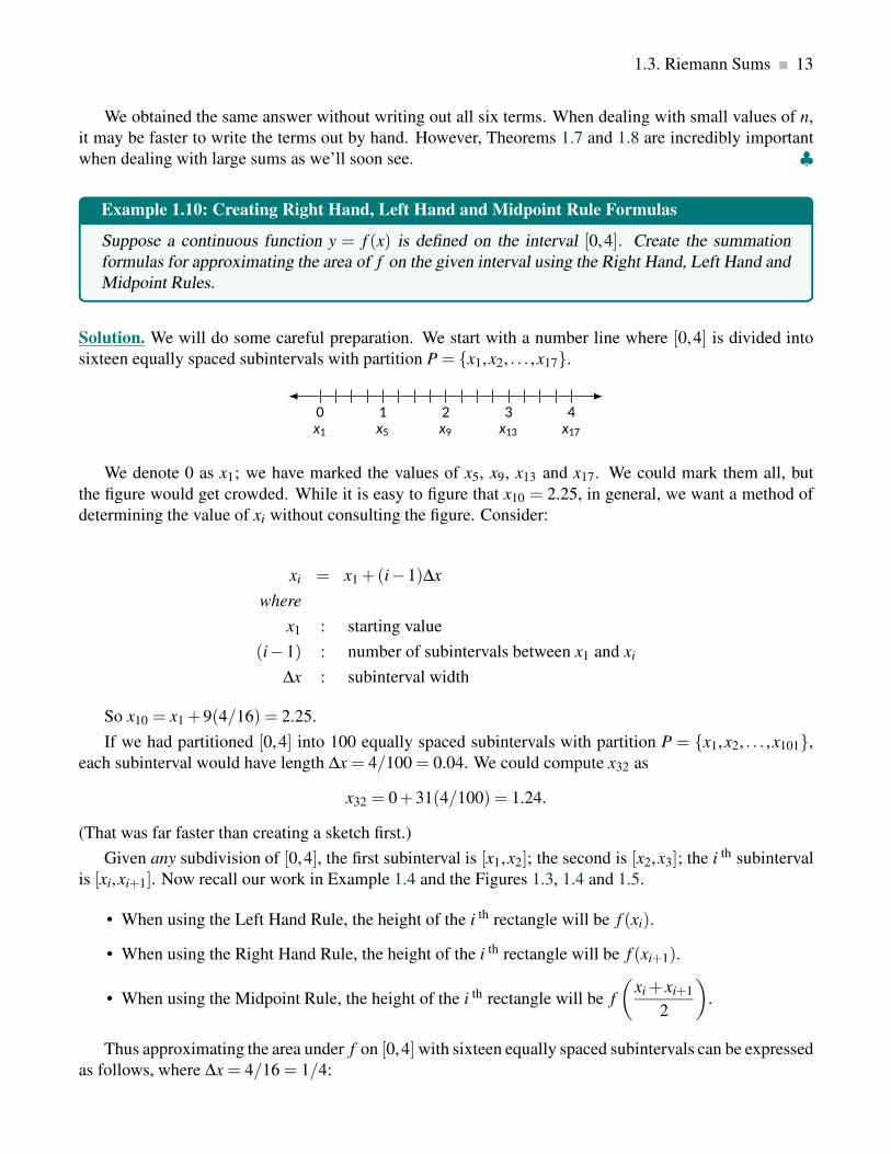
Example 1.10: Creating Right Hand, Left Hand and Midpoint Rule Formulas
Suppose a continuous function y = f (x) is defined on the interval [0,4]. Create the summation
formulas for approximating the area of f on the given interval using the Right Hand, Left Hand and
Midpoint Rules.
Solution. We will do some careful preparation. We start with a number line where [0,4] is divided into
sixteen equally spaced subintervals with partition P = {x1,x2, . . . ,x17}.
0 1 2 3 4
x1 x5 x9 x13 x17
We denote 0 as x1; we have marked the values of x5, x9, x13 and x17. We could mark them all, but
the figure would get crowded. While it is easy to figure that x10 = 2.25, in general, we want a method of
determining the value of xi without consulting the figure. Consider:
xi = x1 +(i−1)∆x
where
x1 : starting value
(i−1) : number of subintervals between x1 and xi
∆x : subinterval width
So x10 = x1 +9(4/16) = 2.25.
If we had partitioned [0,4] into 100 equally spaced subintervals with partition P = {x1,x2, . . . ,x101},
each subinterval would have length ∆x = 4/100 = 0.04. We could compute x32 as
x32 = 0+31(4/100) = 1.24.
(That was far faster than creating a sketch first.)
Given any subdivision of [0,4], the first subinterval is [x1,x2]; the second is [x2,x3]; the i th subinterval
is [xi,xi+1]. Now recall our work in Example 1.4 and the Figures 1.3, 1.4 and 1.5.
• When using the Left Hand Rule, the height of the i th rectangle will be f (xi).
• When using the Right Hand Rule, the height of the i th rectangle will be f (xi+1).
• When using the Midpoint Rule, the height of the i th rectangle will be f
(
xi + xi+1
2
)
.
Thus approximating the area under f on [0,4] with sixteen equally spaced subintervals can be expressed
as follows, where ∆x = 4/16 = 1/4:

14 Integration
Left Hand Rule:16
∑i=1
f (xi) ·1
4
Right Hand Rule:16
∑i=1
f (xi+1) ·1
4
Midpoint Rule:16
∑i=1
f
(
xi + xi+1
2
)
· 1
4
♣
We use these formulas in the following example.
Example 1.11: Approximating Area Using Sums
Approximate the area under f (x) = 4x− x2 on [0,4] using the Right Hand Rule and summation
formulas with sixteen and 1000 equally spaced intervals.
Solution. Using sixteen equally spaced intervals and the Right Hand Rule, we can approximate the area
as16
∑i=1
f (xi+1)∆x.
We have ∆x = 4/16 = 0.25. Since xi = 0+(i−1)∆x, we have
xi+1 = 0+(
(i+1)−1)
∆x
= i∆x
Using the summation formulas, consider:
16
∑i=1
f (xi+1)∆x =16
∑i=1
f (i∆x)∆x
=16
∑i=1
(
4i∆x− (i∆x)2)
∆x
=16
∑i=1
(4i∆x2 − i2∆x3)
= (4∆x2)16
∑i=1
i−∆x316
∑i=1
i2 (1.1)
= (4∆x2)16 ·17
2−∆x3 16(17)(33)
6
= 4 ·0.252 ·136−0.253 ·1496
= 10.625
We were able to sum up the areas of sixteen rectangles with very little computation. The function and
the sixteen rectangles are graphed below. While some rectangles over–approximate the area, other under–
approximate the area (by about the same amount). Thus our approximate area of 10.625 is likely a fairly
good approximation.

1.3. Riemann Sums 15
1 2 3 4
1
2
3
4
x
y
Notice Equation (1.1); by changing the 16’s to 1,000’s (and appropriately changing the value of ∆x),
we can use that equation to sum up 1000 rectangles!
We do so here, skipping from the original summand to the equivalent of Equation (1.1) to save space.
Note that ∆x = 4/1000 = 0.004.
1000
∑i=1
f (xi+1)∆x = (4∆x2)1000
∑i=1
i−∆x31000
∑i=1
i2
= (4∆x2)1000 ·1001
2−∆x3 1000(1001)(2001)
6
= 4 ·0.0042 ·500500−0.0043 ·333,833,500
= 10.666656
Using many, many rectangles, we have a likely good approximation of the area under f (x) = 4x− x2
of ≈ 10.666656. ♣
Before the above example, we stated the summations for the Left Hand, Right Hand and Midpoint
Rules in Example 1.10. Each had the same basic structure, which was:
1. Each rectangle has the same width, which we referred to as ∆x, and
2. Each rectangle’s height is determined by evaluating f (x) at a particular point in each subinterval.
For instance, the Left Hand Rule states that each rectangle’s height is determined by evaluating f (x)at the left hand endpoint of the subinterval the rectangle lives on.
One could partition an interval [a,b] with subintervals that did not have the same width. We refer to
the length of the first subinterval as ∆x1, the length of the second subinterval as ∆x2, and so on, giving the
length of the i th subinterval as ∆xi. Also, one could determine each rectangle’s height by evaluating f (x) at
any point in the i th subinterval. We refer to the point picked in the first subinterval as c1, the point picked
in the second subinterval as c2, and so on, with ci representing the point picked in the i th subinterval. Thus
the height of the i th subinterval would be f (ci), and the area of the i th rectangle would be f (ci)∆xi.
Summations of rectangles with area f (ci)∆xi are named after mathematician Georg Friedrich Bernhard
Riemann, as given in the following definition.

16 Integration
Definition 1.12: Riemann Sum
Let f (x) be defined on the closed interval [a,b] and let P = {x1,x2, . . . ,xn+1} be a partition of [a,b],with
a = x1 < x2 < .. . < xn < xn+1 = b.
Let ∆xi denote the length of the i th subinterval [xi,xi+1] and let ci denote any value in the i th subin-
terval.
The sumn
∑i=1
f (ci)∆xi
is a Riemann sum of f (x) on [a,b].
Riemann sums are typically calculated using one of the three rules we have introduced. The uniformity
of construction makes computations easier. Before working another example, let’s summarize some of
what we have learned in a convenient way.
Riemann Sums Using Rules (Left - Right - Midpoint)
Consider a function f (x) defined on an interval [a,b]. The area under this curve is approximated by
∑ni=1 f (ci)∆xi.
1. When the n subintervals have equal length, ∆xi = ∆x =b−a
n.
2. The i th term of the partition is xi = a+(i−1)∆x. (This makes xn+1 = b.)
3. The Left Hand Rule summation is:n
∑i=1
f (xi)∆x.
4. The Right Hand Rule summation is:n
∑i=1
f (xi+1)∆x.
5. The Midpoint Rule summation is:n
∑i=1
f
(
xi + xx+1
2
)
∆x.
Figure 1.6 shows the approximating rectangles of a Riemann sum. While the rectangles in this example
do not approximate well the shaded area, they demonstrate that the subinterval widths may vary and the
heights of the rectangles can be determined without following a particular rule.

1.3. Riemann Sums 17
1 2 3 4
1
2
3
4
x
y
Figure 1.6: General Riemann sum to approximate the area under f (x) = 4x− x2
Let’s do another example.
Example 1.13: Approximating Area Using Sums
Approximate the area under f (x) = (5x+2) on the interval [−2,3] using the Midpoint Rule and ten
equally spaced intervals.
Solution. Following the above discussion, we have
∆x =3− (−2)
10= 1/2
xi = (−2)+(1/2)(i−1) = i/2−5/2.
As we are using the Midpoint Rule, we will also need xi+1 andxi + xi+1
2. Since xi = i/2− 5/2, xi+1 =
(i+1)/2−5/2 = i/2−2. This gives
xi + xi+1
2=
(i/2−5/2)+(i/2−2)
2=
i−9/2
2= i/2−9/4.
We now construct the Riemann sum and compute its value using summation formulas.
10
∑i=1
f
(
xi + xi+1
2
)
∆x =10
∑i=1
f (i/2−9/4)∆x
=10
∑i=1
(
5(i/2−9/4)+2)
∆x
= ∆x10
∑i=1
[(
5
2
)
i− 37
4
]
= ∆x
(
5
2
10
∑i=1
(i)−10
∑i=1
(
37
4
)
)

18 Integration
=1
2
(
5
2· 10(11)
2−10 · 37
4
)
=45
2= 22.5
Note the graph below of f (x) = 5x+ 2 and its area-approximation using the Midpoint Rule and 10
evenly spaced subintervals. The regions whose areas are computed are triangles, meaning we can find the
exact answer without summation techniques. We find that the exact answer is indeed 22.5. One of the
strengths of the Midpoint Rule is that often each rectangle includes area that should not be counted, but
misses other area that should. When the partition width is small, these two amounts are about equal and
these errors almost “cancel each other out.” In this example, since our function is a line, these errors are
exactly equal and they do cancel each other out, giving us the exact answer.
−1−2
1 2 3
10
17
−8
x
y
Note too that when the function is negative, the rectangles have a “negative” height and a negative
signed area. When we compute the area of the rectangle, we use f (ci)∆x; when f is negative, the area is
counted as negative. ♣
Notice in the previous example that while we used ten equally spaced intervals, the number “10” didn’t
play a big role in the calculations until the very end. Mathematicians love abstract ideas; let’s approximate
the area of another region using n subintervals, where we do not specify a value of n until the very end.
Example 1.14: Approximating Area Using Sums
Revisit f (x) = 4x− x2 on the interval [0,4] yet again. Approximate the area under this curve using
the Right Hand Rule with n equally spaced subintervals.
Solution. We know ∆x = 4−0n = 4/n. We also find xi = 0+∆x(i−1) = 4(i−1)/n. The Right Hand Rule
uses xi+1, which is xi+1 = 4i/n. We construct the Right Hand Rule Riemann sum as follows.
n
∑i=1
f (xi+1)∆x =n
∑i=1
f
(
4i
n
)
∆x

1.3. Riemann Sums 19
=n
∑i=1
[
44i
n−(
4i
n
)2]
∆x
=n
∑i=1
(
16∆x
n
)
i−n
∑i=1
(
16∆x
n2
)
i2
=
(
16∆x
n
) n
∑i=1
i−(
16∆x
n2
) n
∑i=1
i2
=
(
16∆x
n
)
· n(n+1)
2−(
16∆x
n2
)
n(n+1)(2n+1)
6
(
recall
∆x = 4/n
)
=32(n+1)
n− 32(n+1)(2n+1)
3n2(now simplify)
=32
3
(
1− 1
n2
)
The result is an amazing, easy to use formula. To approximate the area with ten equally spaced
subintervals and the Right Hand Rule, set n = 10 and compute
32
3
(
1− 1
102
)
= 10.56.
Recall how earlier we approximated the area with 4 subintervals; with n = 4, the formula gives 10, our
answer as before.
It is now easy to approximate the area with 1,000,000 subintervals! Hand-held calculators will round
off the answer a bit prematurely giving an answer of 10.66666667. (The actual answer is 10.666666666656.)
We now take an important leap. Up to this point, our mathematics has been limited to geometry and
algebra (finding areas and manipulating expressions). Now we apply calculus. For any finite n, we know
that the corresponding Right Hand Rule Riemann sum is:
32
3
(
1− 1
n2
)
.
Both common sense and high–level mathematics tell us that as n gets large, the approximation gets better.
In fact, if we take the limit as n → ∞, we get the exact area. That is,
limn→∞
32
3
(
1− 1
n2
)
=32
3(1−0)
=32
3= 10.6
This is a fantastic result. By considering n equally–spaced subintervals, we obtained a formula for an
approximation of the area that involved our variable n. As n grows large – without bound – the error
shrinks to zero and we obtain the exact area. ♣
This section started with a fundamental calculus technique: make an approximation, refine the approx-
imation to make it better, then use limits in the refining process to get an exact answer. That is precisely
what we just did.

20 Integration
Let’s practice this again.
Example 1.15: Approximating Area With a Formula, Using Sums
Find a formula that approximates the area under f (x) = x3 on the interval [−1,5] using the Right
Hand Rule and n equally spaced subintervals, then take the limit as n → ∞ to find the exact area.
Solution. We have ∆x =5−(−1)
n = 6/n. We have xi = (−1)+(i−1)∆x; as the Right Hand Rule uses xi+1,
we have xi+1 = (−1)+ i∆x.
The Riemann sum corresponding to the Right Hand Rule is (followed by simplifications):
n
∑i=1
f (xi+1)∆x =n
∑i=1
f (−1+ i∆x)∆x
=n
∑i=1
(−1+ i∆x)3∆x
=n
∑i=1
(
(i∆x)3 −3(i∆x)2 +3i∆x−1)
∆x
=n
∑i=1
(
i3∆x4 −3i2∆x3 +3i∆x2 −∆x)
= ∆x4n
∑i=1
i3 −3∆x3n
∑i=1
i2 +3∆x2n
∑i=1
i−n
∑i=1
∆x
= ∆x4
(
n(n+1)
2
)2
−3∆x3 n(n+1)(2n+1)
6+3∆x2 n(n+1)
2−n∆x
=1296
n4· n2(n+1)2
4−3
216
n3· n(n+1)(2n+1)
6+3
36
n2
n(n+1)
2−6
= 156+378
n+
216
n2
Once again, we have found a compact formula for approximating the area with n equally spaced subinter-
vals and the Right Hand Rule. The graph below depicts the graph of f and its area-approximation using
the Right Hand Rule and 10 evenly spaced subintervals. This yields an approximation of 195.96. Using
n = 100 gives an approximation of 159.802.
Ȃ 1 1 2 3 4 5
50
100
x
y

1.3. Riemann Sums 21
Now find the exact answer using a limit:
limn→∞
(
156+378
n+
216
n2
)
= 156.
♣
We have used limits to evaluate exactly given definite limits. Will this always work? We will show,
given not–very–restrictive conditions, that yes, it will always work.
The previous two examples demonstrated how an expression such as
n
∑i=1
f (xi+1)∆x
can be rewritten as an expression explicitly involving n, such as 32/3(1−1/n2).
Viewed in this manner, we can think of the summation as a function of n. An n value is given (where n
is a positive integer), and the sum of areas of n equally spaced rectangles is returned, using the Left Hand,
Right Hand, or Midpoint Rules.
Given a function f (x) defined on the interval [a,b] let:
• SL(n) =n
∑i=1
f (xi)∆x, the sum of equally spaced rectangles formed using the Left Hand Rule,
• SR(n) =n
∑i=1
f (xi+1)∆x, the sum of equally spaced rectangles formed using the Right Hand Rule, and
• SM(n) =n
∑i=1
f
(
xi + xi+1
2
)
∆x, the sum of equally spaced rectangles formed using the Midpoint
Rule.
The following theorem states that we can use any of our three rules to find the exact value of the area
under f (x) on [a,b]. It also goes two steps further. The theorem states that the height of each rectangle
doesn’t have to be determined following a specific rule, but could be f (ci), where ci is any point in the i th
subinterval, as discussed earlier.
The theorem goes on to state that the rectangles do not need to be of the same width. Using the notation
of Definition 1.12, let ∆xi denote the length of the i th subinterval in a partition of [a,b]. Now let ||∆x||represent the length of the largest subinterval in the partition: that is, ||∆x|| is the largest of all the ∆xi’s.
If ||∆x|| is small, then [a,b] must be partitioned into many subintervals, since all subintervals must have
small lengths. “Taking the limit as ||∆x|| goes to zero” implies that the number n of subintervals in the
partition is growing to infinity, as the largest subinterval length is becoming arbitrarily small. We then
interpret the expression
lim||∆x||→0
n
∑i=1
f (ci)∆xi
as “the limit of the sum of rectangles, where the width of each rectangle can be different but getting small,
and the height of each rectangle is not necessarily determined by a particular rule.” The following theorem
states that, for a sufficiently nice function, we can use any of our three rules to find the area under f (x)over [a,b].

22 Integration
Theorem 1.16: Area and the Limit of Riemann Sums
Let f (x) be a continuous function on the closed interval [a,b] and let SL(n), SR(n) and SM(n) be
the sums of equally spaced rectangles formed using the Left Hand Rule, Right Hand Rule, and
Midpoint Rule, respectively. Then:
1. limn→∞
SL(n) = limn→∞
SR(n) = limn→∞
SM(n) = limn→∞
n
∑i=1
f (ci)∆xi
2. The net area under f on the interval [a,b] is equal to limn→∞
n
∑i=1
f (ci)∆xi.
3. The net area under f on the interval [a,b] is equal to lim‖∆x‖→0
n
∑i=1
f (ci)∆xi.
We summarize what we have learned over the past few sections here.
• Knowing the “area under the curve” can be useful. One common example is: the area under a
velocity curve is displacement.
• While we can approximate the area under a curve in many ways, we have focused on using rectangles
whose heights can be determined using: the Left Hand Rule, the Right Hand Rule and the Midpoint
Rule.
• Sums of rectangles of this type are called Riemann sums.
• The exact value of the area can be computed using the limit of a Riemann sum. We generally use
one of the above methods as it makes the algebra simpler.
Exercises for Section 1.3
Exercise 1.3.1 Find the area under y = 2x between x = 0 and any positive value for x.
Exercise 1.3.2 Find the area under y = 4x between x = 0 and any positive value for x.
Exercise 1.3.3 Find the area under y = 4x between x = 2 and any positive value for x bigger than 2.
Exercise 1.3.4 Find the area under y = 4x between any two positive values for x, say a < b.
Exercise 1.3.5 Let f (x) = x2 + 3x+ 2. Approximate the area under the curve between x = 0 and x = 2
using 4 rectangles and also using 8 rectangles.
Exercise 1.3.6 Let f (x) = x2 − 2x+ 3. Approximate the area under the curve between x = 1 and x = 3
using 4 rectangles.

1.4. The Definite Integral and FTC 23
1.4 The Definite Integral and FTC
1.4.1. Exploring an Example
We begin by exploring an example. Suppose that an object moves in a straight line so that its speed is 3t
at time t. How far does the object travel between time t = a and time t = b? We don’t assume that we
know where the object is at time t = 0 or at any other time. It is certainly true that it is somewhere, so
let’s suppose that at t = 0 the position is k. Then we know that the position of the object at any time is
3t2/2+k. This means that at time t = a the position is 3a2/2+k and at time t = b the position is 3b2/2+k.
Therefore the change in position is 3b2/2+k− (3a2/2+k) = 3b2/2−3a2/2. Notice that the k drops out;
this means that it doesn’t matter that we don’t know k, it doesn’t even matter if we use the wrong k, we get
the correct answer.
What about a second approach to this problem? We now want to approximate the change in position
between time a and time b. We take the interval of time between a and b, divide it into n subintervals,
and approximate the distance traveled during each. The starting time of subinterval number i is now
a+(i−1)(b−a)/n, which we abbreviate as ti−1, so that t0 = a, t1 = a+(b−a)/n, and so on. The speed
of the object is f (t) = 3t, and each subinterval is (b− a)/n = ∆t seconds long. The distance traveled
during subinterval number i is approximately f (ti−1)∆t, and the total change in distance is approximately
f (t0)∆t + f (t1)∆t + · · ·+ f (tn−1)∆t.
The exact change in position is the limit of this sum as n goes to infinity. We abbreviate this sum using
sigma notation:n−1
∑i=0
f (ti)∆t = f (t0)∆t + f (t1)∆t + · · ·+ f (tn−1)∆t.
The answer we seek is
limn→∞
n−1
∑i=0
f (ti)∆t.
Since this must be the same as the answer we have already obtained, we know that
limn→∞
n−1
∑i=0
f (ti)∆t =3b2
2− 3a2
2.
The significance of 3t2/2, into which we substitute t = b and t = a, is of course that it is a function whose
derivative is f (t). As we have discussed, by the time we know that we want to compute
limn→∞
n−1
∑i=0
f (ti)∆t,
it no longer matters what f (t) stands for—it could be a speed, or the height of a curve, or something else
entirely. We know that the limit can be computed by finding any function with derivative f (t), substituting
a and b, and subtracting. We summarize this result in a theorem in Section 1.4.3 The Fundamental Theo-
rem of Calculus, but first, we introduce the new notation definite integral and the terminology associated
with it.

24 Integration
1.4.2. Defining the Definite Integral
Definition 1.17: The Definite Integral
Let f be a continuous function defined on the interval [a,b] with partition P = {t0, t1, . . . , tn} of [a,b]and subinterval width ∆t. If the limit
limn→∞
n−1
∑i=0
f (ti)∆t
exists, then the definite integral of f over [a,b] is defined by
∫ b
af (t)dt = lim
n→∞
n−1
∑i=0
f (ti)∆t
where∫ b
af (t)dt is read “the integral of f from a to b,
the symbol∫
is called the integral sign,
the value a is the lower limit of integration,
the value b is the upper limit of integration,
the function f is referred to as the integrand of the integral, and
the variable t is called the variable of integration.
Note:
1. The process of finding the definite integral is called integration or integrating f (x).
2. If the definite integral of f exists over [a,b], then the function f is integrable on [a,b].
3. The definite integral is a number and not a function.
4. The value of the definite integral is independent of the variable of integration. Whether the integral
is written as∫ b
af (x)dx or
∫ b
af (t)dt or
∫ b
af (u)du,
it is still the limit of Riemann sums yielding the same value. Hence, the variable of integration is
sometimes referred to as a dummy variable.
5. If f is non-negative, then the definite integral represents the area of the region under the graph of f
on [a,b]; otherwise, the definite integral represents the net area of the regions under the graph of f
on [a,b], which we will summarize in the geometric interpretation below.
We should ask ourselves, when is a function integrable? It turns out that no matter what choices are
made in the Riemann sums associated with a continuous function, the Riemann sums always converge to
the same limit. This is stated in the following theorem, which we will not prove.

1.4. The Definite Integral and FTC 25
Theorem 1.18: Existence of a Definite Integral
A continuous function on [a,b] is integrable over [a,b].
Just like we emphasized the geometric interpretation of the derivative, we do not want to lose sight of
the geometric interpretation of the definite integral.
Geometric Interpretation of the Definite Integral – Area versus Net Area
Suppose f is continuous on the interval [a,b], then
∫ b
af (x)dx
represents
1. the area of the region under the graph of f on [a,b] if f is non-negative, and otherwise
a b
y = f (x)
Area=
∫ b
af (x)dx
x
y
2. the net area of the region under the graph of f on [a,b].
a b
y = f (x)A1
A2
A3
∫ b
af (x)dx = A1 −A2 +A3
x
y

26 Integration
Lastly, we conclude this section by listing the properties of the definite integral.
Properties of Definite Integrals
Order of limits matters:
∫ b
af (x)dx =−
∫ a
bf (x)dx
If interval is empty, integral is zero:
∫ a
af (x)dx = 0
Constant Multiple Rule:
∫ b
ac f (x)dx = c
∫ b
af (x)dx
Sum/Difference Rule:
∫ b
a[ f (x)±g(x)] dx =
∫ b
af (x)dx±
∫ b
ag(x)dx
Can split up interval [a,b] = [a,c]∪ [c,b]:
∫ b
af (x)dx =
∫ c
af (x)dx+
∫ b
cf (x)dx
The variable does not matter:
∫ b
af (x)dx =
∫ b
af (t)dt
The reason for the last property is that a definite integral is a number, not a function, so the variable is
just a placeholder that won’t appear in the final answer.
Some additional properties are comparison types of properties.
Comparison Properties of Definite Integrals
If f (x)≥ 0 for x ∈ [a,b], then
∫ b
af (x)dx ≥ 0.
If f (x)≥ g(x) for x ∈ [a,b], then
∫ b
af (x)dx ≥
∫ b
ag(x)dx.
If m ≤ f (x)≤ M for x ∈ [a,b], then m(b−a)≤∫ b
af (x)dx ≤ M(b−a).
Example 1.19: Properties of Definite Integrals
Suppose
∫ b
af (x) dx = 7 and
∫ b
ag(x) dx = 3. Find:
(a)
∫ b
a2 f (x)−3g(x)dx.
(b)
∫ a
b2g(x)dx.
(c)
∫ a
af (x) ·g(x)dx.
(d)
∫ c
af (x) dx+
∫ b
cf (x)dx.
Solution.
(a)
∫ b
a2 f (x)−3g(x)dx = 2
∫ b
af (x)dx−3
∫ b
ag(x)dx = 2(7)−3(3) = 5.
(b)
∫ a
b2g(x)dx =−2
∫ b
ag(x)dx =−2(3) =−6.

1.4. The Definite Integral and FTC 27
(c)
∫ a
af (x) ·g(x)dx = 0.
(d)
∫ c
af (x)dx+
∫ b
cf (x)dx =
∫ b
af (x)dx = 7.
♣
1.4.3. The Fundamental Theorem of Calculus
We are finally in a position to state the result from our exploration at the beginning of Section 1.4.1. What
we have learned is that the integral of f over the interval [a,b] can be computed by finding a function, say
F(t), with the property that F ′(t) = f (t), and then computing F(b)−F(a). Recall that the function F(t)is called an antiderivative of f (t). Let us now state the theorem:
Theorem 1.20: Fundamental Theorem of Calculus
Suppose that f (x) is continuous on the interval [a,b]. If F(x) is any antiderivative of f (x), then
∫ b
af (x)dx = F(b)−F(a).
Let’s rewrite this slightly:∫ x
af (t)dt = F(x)−F(a).
We’ve replaced the variable x by t and b by x. These are just different names for quantities, so the
substitution doesn’t change the meaning of the theorem statement. However, it does allow us to give a
new interpretation of the theorem by thinking of the two sides of the equation as functions of x. The
expression∫ x
af (t)dt
is a function: plug in a value for x, get out some other value. The expression F(x)−F(a) is of course also
a function, and it has a nice property:
d
dx(F(x)−F(a)) = F ′(x) = f (x),
since F(a) is a constant and has derivative zero. In other words, by shifting our point of view slightly, we
see that the odd looking function
G(x) =
∫ x
af (t)dt
has a derivative, and that in fact G′(x) = f (x).
Note: This is really just a restatement of the Fundamental Theorem of Calculus, and indeed is often called
the Fundamental Theorem of Calculus. To avoid confusion, some people call the two versions of the
theorem “The Fundamental Theorem of Calculus, part I” and “The Fundamental Theorem of Calculus, part

28 Integration
II”, although unfortunately there is no universal agreement as to which is part I and which part II. Since
it really is the same theorem, differently stated, some people simply call them both “The Fundamental
Theorem of Calculus.”
Theorem 1.21: Fundamental Theorem of Calculus
Suppose that f (x) is continuous on the interval [a,b] and let
G(x) =∫ x
af (t)dt.
Then G′(x) = f (x).
We have not really proved the Fundamental Theorem. In a nutshell, we gave the following argument
to justify it: Suppose we want to know the value of
∫ b
af (t)dt = lim
n→∞
n−1
∑i=0
f (ti)∆t.
We can interpret the right hand side as the distance traveled by an object whose speed is given by f (t). We
know another way to compute the answer to such a problem: find the position of the object by finding an
antiderivative of f (t), then substitute t = a and t = b and subtract to find the distance traveled. This must
be the answer to the original problem as well, even if f (t) does not represent a speed.
What’s wrong with this? In some sense, nothing. As a practical matter it is a very convincing argument,
because our understanding of the relationship between speed and distance seems to be quite solid. From
the point of view of mathematics, however, it is unsatisfactory to justify a purely mathematical relationship
by appealing to our understanding of the physical universe, which could, however unlikely it is in this case,
be wrong.
A complete proof is a bit too involved to include here, but we will indicate how it goes. First, if we
can prove the second version of the Fundamental Theorem of Calculus, Theorem 1.21, then we can prove
the first version from that:
Proof. Proof of Theorem 1.20.
We know from Theorem 1.21 that
G(x) =
∫ x
af (t)dt
is an antiderivative of f (x), and therefore any antiderivative F(x) of f (x) is of the form F(x) = G(x)+ k.
Then
F(b)−F(a) = G(b)+ k− (G(a)+ k) = G(b)−G(a)
=
∫ b
af (t)dt −
∫ a
af (t)dt.
It is clear that
∫ a
af (t)dt = 0, so this means that
F(b)−F(a) =
∫ b
af (t)dt,

1.4. The Definite Integral and FTC 29
which is exactly what Theorem 1.20 says. ♣
So the real job is to prove Theorem 1.21. We will sketch the proof, using some facts that we do not
prove. First, the following identity is true of integrals:
∫ b
af (t)dt =
∫ c
af (t)dt+
∫ b
cf (t)dt.
This can be proved directly from the definition of the integral, that is, using the limits of sums. It is quite
easy to see that it must be true by thinking of either of the two applications of integrals that we have seen.
It turns out that the identity is true no matter what c is, but it is easiest to think about the meaning when
a ≤ c ≤ b.
First, if f (t) represents a speed, then we know that the three integrals represent the distance traveled
between time a and time b; the distance traveled between time a and time c; and the distance traveled
between time c and time b. Clearly the sum of the latter two is equal to the first of these.
Second, if f (t) represents the height of a curve, the three integrals represent the area under the curve
between a and b; the area under the curve between a and c; and the area under the curve between c and b.
Again it is clear from the geometry that the first is equal to the sum of the second and third.
Proof. Proof of Theorem 1.21.
We want to compute G′(x), so we start with the definition of the derivative in terms of a limit:
G′(x) = lim∆x→0
G(x+∆x)−G(x)
∆x
= lim∆x→0
1
∆x
(
∫ x+∆x
af (t)dt−
∫ x
af (t)dt
)
= lim∆x→0
1
∆x
(
∫ x
af (t)dt+
∫ x+∆x
xf (t)dt−
∫ x
af (t)dt
)
= lim∆x→0
1
∆x
∫ x+∆x
xf (t)dt.
Now we need to know something about∫ x+∆x
xf (t)dt
when ∆x is small; in fact, it is very close to ∆x f (x), but we will not prove this. Once again, it is easy to
believe this is true by thinking of our two applications: The integral
∫ x+∆x
xf (t)dt
can be interpreted as the distance traveled by an object over a very short interval of time. Over a sufficiently
short period of time, the speed of the object will not change very much, so the distance traveled will be
approximately the length of time multiplied by the speed at the beginning of the interval, namely, ∆x f (x).Alternately, the integral may be interpreted as the area under the curve between x and x+∆x. When ∆x is
very small, this will be very close to the area of the rectangle with base ∆x and height f (x); again this is
∆x f (x). If we accept this, we may proceed:
lim∆x→0
1
∆x
∫ x+∆x
xf (t)dt = lim
∆x→0
∆x f (x)
∆x= f (x),

30 Integration
which is what we wanted to show. ♣
It is still true that we are depending on an interpretation of the integral to justify the argument, but
we have isolated this part of the argument into two facts that are not too hard to prove. Once the last
reference to interpretation has been removed from the proofs of these facts, we will have a real proof of
the Fundamental Theorem of Calculus.
Note: Now we know that to solve certain kinds of problems, those that lead to a sum of a certain form, we
“merely” find an antiderivative and substitute two values and subtract. Unfortunately, finding antideriva-
tives can be quite difficult. While there are a small number of rules that allow us to compute the derivative
of any common function, there are no such rules for antiderivatives. There are some techniques that fre-
quently prove useful as you will see in Chapter 2 Techniques of Integration, but we will never be able to
reduce the problem to a completely mechanical process.
1.4.4. Notation when Computing a Definite Integral
When we compute a definite integral, we first find an antiderivative of the integrand and then substitute. It
is convenient to first display the antiderivative and then do the substitution; we need a notation indicating
that the substitution is yet to be done. A typical solution would look like this:
∫ 2
1x2 dx =
x3
3
∣
∣
∣
∣
2
1
=23
3− 13
3=
7
3.
The vertical line with subscript and superscript is used to indicate the operation “substitute and subtract”
that is needed to finish the evaluation.
Common Mistakes:
1. Dropping the dx at the end of the integral. This is required! Think of the integral as a set of
parenthesis consisting of the integral sign and the dx. Both are required so it is clear where the
integrand ends and what variable you are integrating with respect to.
∫ b
af (x)dx 6=
∫ b
af (x)
2. Checking the antiderivative for the integrand using differentiation before following through on the
lower and upper bounds of integration.
∫ b
af (x)dx = F(x)
∣
∣
∣
∣
b
a
with F ′(x) = f (x)
3. Dropping the lower and upper bounds of integration during the solution process. For example:
∫ 2
1x2dx 6=
∫
x2dx 6= x3
3
∣
∣
∣
∣
2
1
=23
3− 13
3=
7
3

1.4. The Definite Integral and FTC 31
4. Forgetting to evaluate using the lower and upper bounds of integration that lead to the value of the
definite integral and instead producing a function. See the note immediately after the definition of
the definite integral. For example:∫ 2
1x2dx 6= x3
3
5. Switching the order in which the lower and upper bounds of integration are being dealt with. For
example:∫ 2
1x2dx =
x
3
∣
∣
∣
∣
2
1
6= 13
3− 23
3=−7
3, or
∫ 2
1x2dx 6= x
3
∣
∣
∣
∣
1
2
=13
3− 23
3=−7
3.
1.4.5. Computing a Definite Integral
We seem to have found a pattern when dealing with power functions. When attempting to solve a previous
question, we found the antiderivative of x2 to be x3/3+ c (as it was when solving the indefinite integral).
Likewise, when we first began, we were trying to determine a position based on velocity, and 3t gave rise
to 3t2/2+ k.
As will be formalized later, we see that in these cases, the power is increased to n+ 1, but we also
divide through by this factor, n+ 1. So the antiderivative of x becomes x2/2, the antiderivative of x2
becomes x3/3, and the antiderivative of x3 will become x4/4.
Now we will also try with negative and fractional values in the following example.
Example 1.22: Fundamental Theorem of Calculus
Evaluate
∫ 4
1
(
x3 +√
x+1
x2
)
dx.
Solution.∫ 4
1
(
x3 +√
x+1
x2
)
dx =x4
4+
2x3/2
3− x−1
∣
∣
∣
∣
∣
4
1
=
(
(4)4
4+
2(4)3/2
3−4−1
)
−(
(1)4
4+
2(1)3/2
3−1−1
)
=415
6

32 Integration
♣
Note: The above integral used parentheses around the integrand for clarity, but we can leave them out
once we are familiar with the notation as shown in the next example.
We next evaluate a definite integral using three different techniques.
Example 1.23: Three Different Techniques
Evaluate
∫ 2
0x+1 dx by
(a) Using FTC II (the shortcut)
(b) Using the definition of a definite integral (the limit sum definition)
(c) Interpreting the problem in terms of areas (graphically)
Solution.
(a) The shortcut (FTC II) is the method of choice as it is the fastest. Integrating and using the ‘top minus
bottom’ rule we have:
∫ 2
0x+1 dx =
x2
2+ x
∣
∣
∣
∣
2
0
=
[
22
2+2
]
−[
02
2+0
]
= 4.
(b) We now use the definition of a definite integral. We divide the interval [0,2] into n subintervals of
equal width ∆x, and from each interval choose a point x∗i . Using the formulas
∆x =b−a
nand xi = a+ i∆x,
we have
∆x =2
nand xi = 0+ i∆x =
2i
n.
Then taking x∗i ’s as right endpoints for convenience (so that x∗i = xi), we have:
∫ 2
0x+1 dx = lim
n→∞
n
∑i=1
f (x∗i )∆x
= limn→∞
n
∑i=1
f
(
2i
n
)
2
n
= limn→∞
n
∑i=1
(
2i
n+1
)
2
n
= limn→∞
n
∑i=1
(
4i
n2+
2
n
)

1.4. The Definite Integral and FTC 33
= limn→∞
(
n
∑i=1
4i
n2+
n
∑i=1
2
n
)
= limn→∞
(
4
n2
n
∑i=1
i+2
n
n
∑i=1
1
)
= limn→∞
(
4
n2
n(n+1)
2+
2
nn
)
= limn→∞
(
2+2
n+2
)
= 4.
(c) Finally, let’s evaluate the net area under x+1 from 0 to 2.
�
� ���������
����
� � �� �
�
�
�
�
�
� ���������
� � �� �
�
�
�
�
Thus, the area is the sum of the areas of a rectangle and a triangle. Hence,
∫ 2
0x+1 dx = Net Area
= Area of rectangle+Area of triangle
= (2)(1)+1
2(2)(2)
= 4.
♣
Example 1.24: FTC and Marginal Profit
A small bakery determines that the marginal profit function for selling q loaves of bread is
P′(q) =−0.0005q2 +2.5
dollars per day per loaf. If the fixed production cost is $10,
(a) determine P(50), and
(b) determine whether or not it is advisable to increase production from 50 loaves to 100 loaves.

34 Integration
Solution.
(a) We first notice that∫ 50
aP′(q)dq = P(50)−P(a).
Since we know that P(0) =−10 (the fixed cost), we take a = 0 and integrate:
∫ 50
0P′(q)dq =
∫ 50
0
(
−0.0005q2 +2.5)
dq
=−0.0005
∫ 50
0q2dq+2.5
∫ 50
0dq
=−0.0005q3
3
∣
∣
∣
∣
50
0
+2.5q
∣
∣
∣
∣
50
0
=−0.0005
(
503
3−0
)
+2.5(50−0)
= 104.167
Thus,
P(50) = 104.167− (−10) = 114.167.
Therefore, the daily profit the bakery realizes from selling 50 loaves of bread is approximately $114.
(b) The change in the profit can be determined by integrating
∫ 100
50P′(q)dq =
∫ 100
50
(
−0.0005q2 +2.5)
dq
=−0.0005
(
1003
3− 503
3
)
+2.5(100−50)
=−20.8333
This means that the bakery would lose about $21 per day if production were doubled. Therefore it
is not advisable to increase production to 100 loaves.
♣We next apply FTC to differentiate a function.
Example 1.25: Using FTC
Differentiate the following function:
g(x) =∫ x
−2cos(1+5t)sint dt.
Solution. We simply apply the Fundamental Theorem of Calculus directly to get:
g′(x) = cos(1+5x)sinx.

1.4. The Definite Integral and FTC 35
♣
Using the Chain Rule we can derive a formula for some more complicated problems when the upper
limit of integration is some function of x rather than simply x. We have:
d
dx
∫ v(x)
af (t)dt = f (v(x)) · v′(x).
Now what if the upper limit is constant and the lower limit is a function of x? Then we interchange the
limits and add a minus sign to get:
d
dx
∫ a
u(x)f (t)dt =− d
dx
∫ u(x)
af (t)dt =− f (u(x)) ·u′(x).
Combining these two we can get a formula where both limits are functions of x. We break up the
integral as follows:∫ v(x)
u(x)f (t)dt =
∫ a
u(x)f (t)dt +
∫ v(x)
af (t)dt.
We just need to make sure f (a) exists after we break up the integral. Then differentiating and using the
above two formulas gives:
FTC and Chain Rule Formula:
d
dx
∫ v(x)
u(x)f (t)dt = f (v(x))v′(x)− f (u(x))u′(x)
Many textbooks do not show this formula and instead to solve these types of problems will use FTC I
along with the tricks we used to derive the formula above. Either method is perfectly fine.
Example 1.26: FTC and Chain Rule
Differentiate the following integral:
∫ x2
10xt3 sin(1+ t)dt.
Solution. We will use the formula above. We have f (t) = t3 sin(1+ t), u(x) = 10x and v(x) = x2. Then
u′(x) = 10 and v′(x) = 2x. Thus,
d
dx
∫ x2
10xt3 sin(1+ t)dt = (x2)3 sin(1+(x2))(2x)− (10x)3 sin(1+(10x))(10)
= 2x7 sin(1+ x2)−10000x3 sin(1+10x)
♣
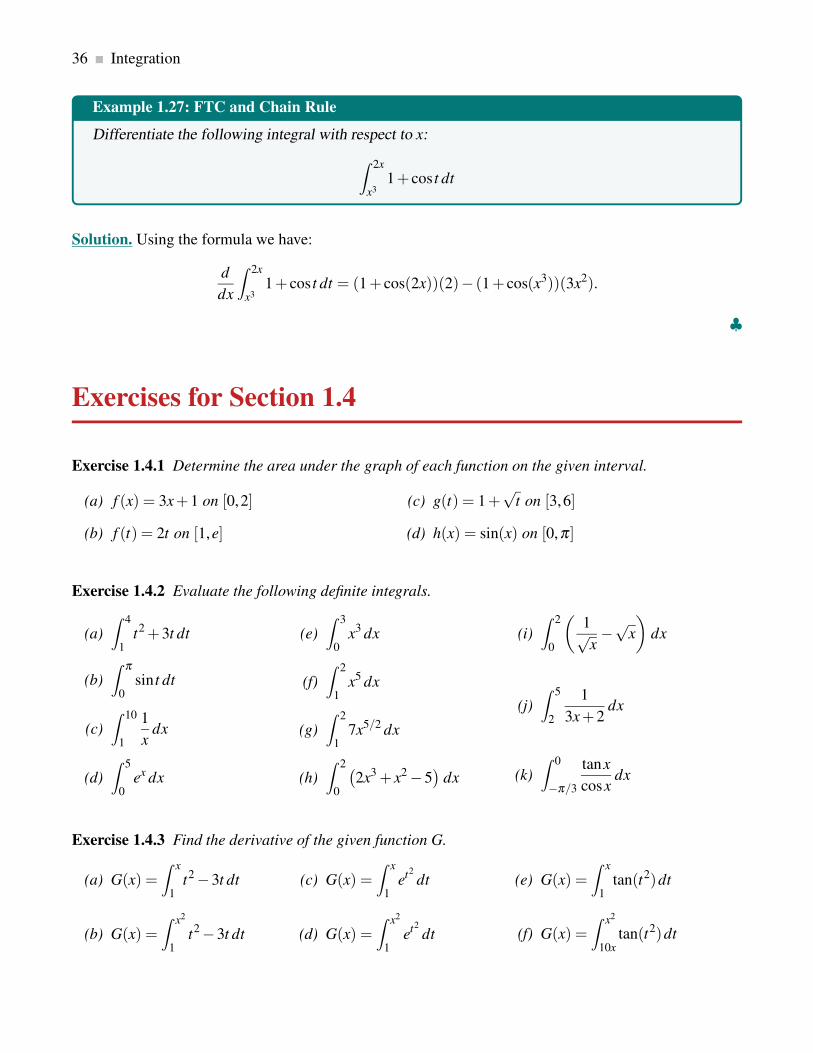
36 Integration
Example 1.27: FTC and Chain Rule
Differentiate the following integral with respect to x:
∫ 2x
x31+ cos t dt
Solution. Using the formula we have:
d
dx
∫ 2x
x31+ cos t dt = (1+ cos(2x))(2)− (1+ cos(x3))(3x2).
♣
Exercises for Section 1.4
Exercise 1.4.1 Determine the area under the graph of each function on the given interval.
(a) f (x) = 3x+1 on [0,2]
(b) f (t) = 2t on [1,e]
(c) g(t) = 1+√
t on [3,6]
(d) h(x) = sin(x) on [0,π ]
Exercise 1.4.2 Evaluate the following definite integrals.
(a)
∫ 4
1t2+3t dt
(b)
∫ π
0sint dt
(c)
∫ 10
1
1
xdx
(d)
∫ 5
0ex dx
(e)
∫ 3
0x3 dx
(f)
∫ 2
1x5 dx
(g)
∫ 2
17x5/2 dx
(h)
∫ 2
0
(
2x3 + x2 −5)
dx
(i)
∫ 2
0
(
1√x−√
x
)
dx
(j)
∫ 5
2
1
3x+2dx
(k)
∫ 0
−π/3
tanx
cosxdx
Exercise 1.4.3 Find the derivative of the given function G.
(a) G(x) =
∫ x
1t2 −3t dt
(b) G(x) =
∫ x2
1t2−3t dt
(c) G(x) =
∫ x
1et2
dt
(d) G(x) =
∫ x2
1et2
dt
(e) G(x) =
∫ x
1tan(t2)dt
(f) G(x) =∫ x2
10xtan(t2)dt

1.5. Indefinite Integrals 37
Exercise 1.4.4 Suppose
∫ 4
1f (x)dx = 2 and
∫ 4
1g(x)dx = 7. Find
∫ 4
1(5 f (x)+3g(x))dx and
∫ 4
1(6−2 f (x))dx.
Exercise 1.4.5 Suppose
∫ 5
−2f (x)dx = 3 and
∫ 5
1f (x)dx =−2. Find
∫ 1
−2f (x)dx.
Exercise 1.4.6 Suppose
∫ 1
−1f (x)dx = 10 and
∫ 1
0f (x)dx = 2. Find
∫ 0
−12 f (x)dx.
Exercise 1.4.7 A manufacturer determines that the marginal cost function associated with the production
of q units is
C′(q) = 0.0006q2−0.5q+25
dollars per unit per day. Suppose the daily fixed cost is $100.
(a) Determine the total cost of producing 30 units.
(b) After 30 units have been made, determine the cost of producing an additional 20 units.
Exercise 1.4.8 A manufacturer determines that the marginal revenue function associated with the pro-
duction of q units is
R′(q) =−0.5q+100
dollars per unit per day.
(a) Determine the total revenue from selling 100 units.
(b) After 100 units have been made, determine the revenue from selling an additional 100 units.
1.5 Indefinite Integrals
In this section we focus on the indefinite integral: its definition, the differences between the definite and
indefinite integrals, some basic integral rules, and how to compute a definite integral.
1.5.1. Defining the Indefinite Integral
Recall the definition of the antiderivative from Section 1.1: A function F is an antiderivative of f on an
interval I if F ′(x) = f (x) for all x in I. Let us explore the antiderivative concretely by letting f (x) = 2x.
Then we can readily determine that the antiderivative of f is the function F(x) = x2, i.e. F ′(x) = f (x).However, the function F(x)+1 = x2 +1 also has f as its derivative:
d
dx(F(x)+1) =
d
dx
(
x2 +1)
= 2x.

38 Integration
In fact, any function F(x)+C = x2 +C for some real constant C has f as its derivative:
d
dx(F(x)+C) =
d
dx
(
x2 +C)
= 2x.
It comes as no surprise to us that the graphs of the family of functions F(x)+C are visually just vertical
displacements of F(x). In the particular case when F(x) = x2, we can also see that the graphs of the family
of functions F(x)+C below that at any point x the tangent lines are parallel, i.e. the tangent slopes are the
same, i.e. the family of functions has the same derivative f (x) = 2x:
x2
x2 +2
x2 −2
x
y
This leads us to the following result:
Definition 1.28: General Antiderivative
If a function F is an antiderivative of f on an interval I, then the most general antiderivative of f
on an interval I is
F(x)+C
where C is any real constant.
Let us now define the indefinite integral.

1.5. Indefinite Integrals 39
Definition 1.29: The Indefinite Integral
The set of all antiderivatives of a function f (x) is the indefinite integral of f (x) with respect to x
and denoted by∫
f (x)dx,
where∫
f (x)dx is read “the integral of f ”
the symbol
∫
is called the integral sign,
the function f is referred to as the integrand of the integral, and
the variable x is called the variable of integration.
Note:
1. The process of finding the indefinite integral is also called integration or integrating f (x).
2. The above definition says that if a function F is an antiderivative of f , then∫
f (x)dx = F(x)+C
for some real constant C.
3. Unlike the definite integral, the indefinite integral is a function.
1.5.2. Definite Integral versus Indefinite Integral
Due to the close relationship between an integral and an antiderivative, the integral sign is also used to
mean “antiderivative”. You can tell which is intended by whether the limits of integration are included:∫ 2
1x2 dx
is an ordinary integral, also called a definite integral, because it has a definite value, namely
∫ 2
1x2 dx =
23
3− 13
3=
7
3.
We use∫
x2 dx
to denote the antiderivative of x2, also called an indefinite integral. So this is evaluated as
∫
x2 dx =x3
3+C,
which is clearly a function as opposed to the definite integral which is a value. It is customary to include
the constant C to indicate that there are really an infinite number of antiderivatives. We do not need this C
to compute definite integrals, but in other circumstances we will need to remember that the C is there, so
it is best to get into the habit of writing the C.

40 Integration
1.5.3. Computing Indefinite Integrals
We are finally ready to compute some indefinite integrals and introduce some basic integration rules from
our knowledge of derivatives. We will first point out some common mistakes frequently observed in
student work.
Common Mistakes:
1. Dropping the dx at the end of the integral. This is required! Think of the integral as a set of
parenthesis consisting of the integral sign and the dx. Both are required so it is clear where the
integrand ends and what variable you are integrating with respect to.
∫
f (x)dx 6=∫
f (x)
2. Forgetting the +C during the solution process and thereby not showing that the solution of an indef-
inite integration process is the set of all antiderivatives of the integrand. As an aside, constants of
integration play a major role in the topic of Differential Equations. For example:
∫
x2dx 6= x3
3
Caution: Note that we don’t have properties to deal with products or quotients of functions, that is,
∫
f (x) ·g(x)dx 6=∫
f (x)dx
∫
g(x)dx.
∫
f (x)
g(x)dx 6=
∫
f (x)dx∫
g(x)dx.
With derivatives, we had the product and quotient rules to deal with these cases. For integrals, we have no
such rules, but we will learn a variety of different techniques to deal with these cases.
The following integral rules can be proved by taking the derivative of the functions on the right side.
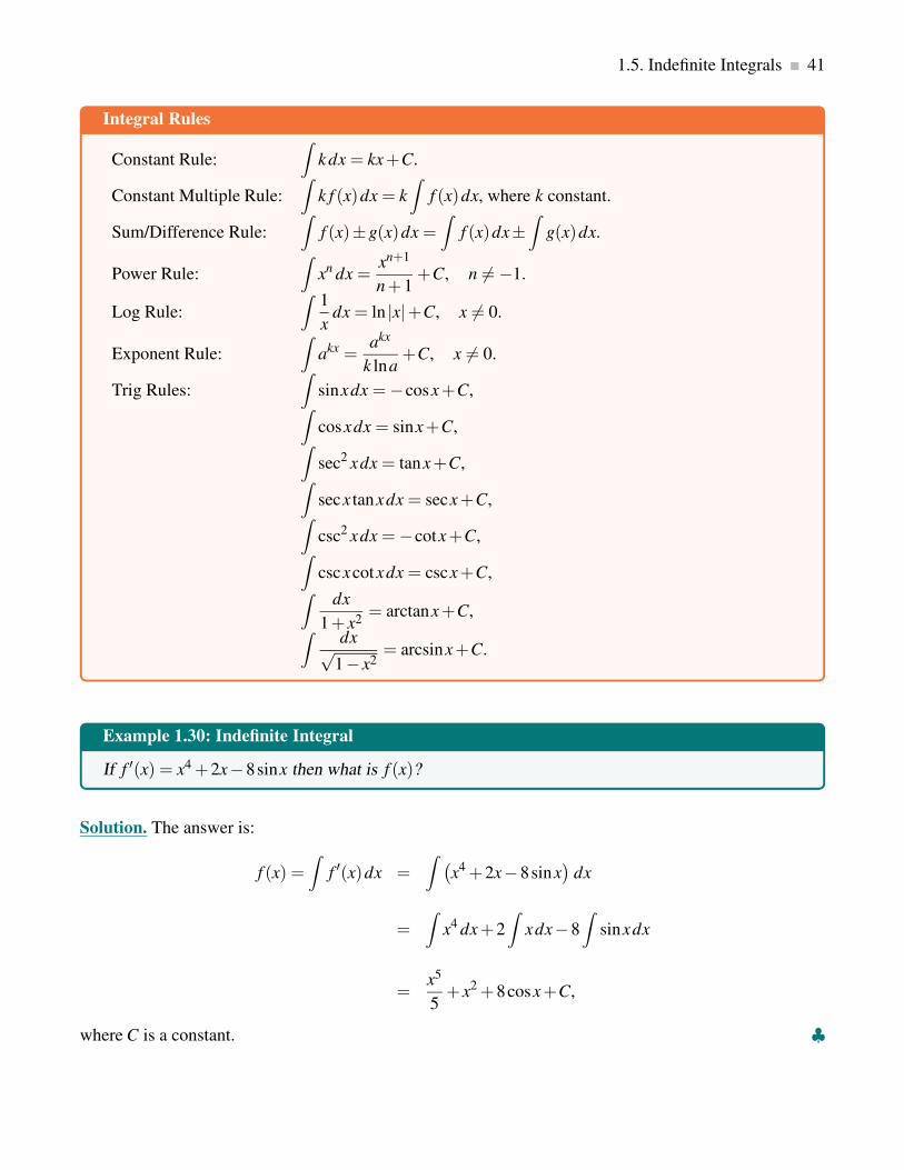
1.5. Indefinite Integrals 41
Integral Rules
Constant Rule:
∫
k dx = kx+C.
Constant Multiple Rule:
∫
k f (x)dx = k
∫
f (x)dx, where k constant.
Sum/Difference Rule:
∫
f (x)±g(x)dx =∫
f (x)dx±∫
g(x)dx.
Power Rule:
∫
xn dx =xn+1
n+1+C, n 6=−1.
Log Rule:
∫
1
xdx = ln |x|+C, x 6= 0.
Exponent Rule:
∫
akx =akx
k lna+C, x 6= 0.
Trig Rules:
∫
sinxdx =−cosx+C,∫
cosxdx = sinx+C,∫
sec2 xdx = tanx+C,∫
secx tanxdx = secx+C,∫
csc2 xdx =−cotx+C,∫
cscxcotxdx = cscx+C,∫
dx
1+ x2= arctanx+C,
∫
dx√1− x2
= arcsinx+C.
Example 1.30: Indefinite Integral
If f ′(x) = x4 +2x−8sinx then what is f (x)?
Solution. The answer is:
f (x) =
∫
f ′(x)dx =
∫
(
x4 +2x−8sinx)
dx
=∫
x4 dx+2
∫
xdx−8
∫
sinxdx
=x5
5+ x2 +8cosx+C,
where C is a constant. ♣
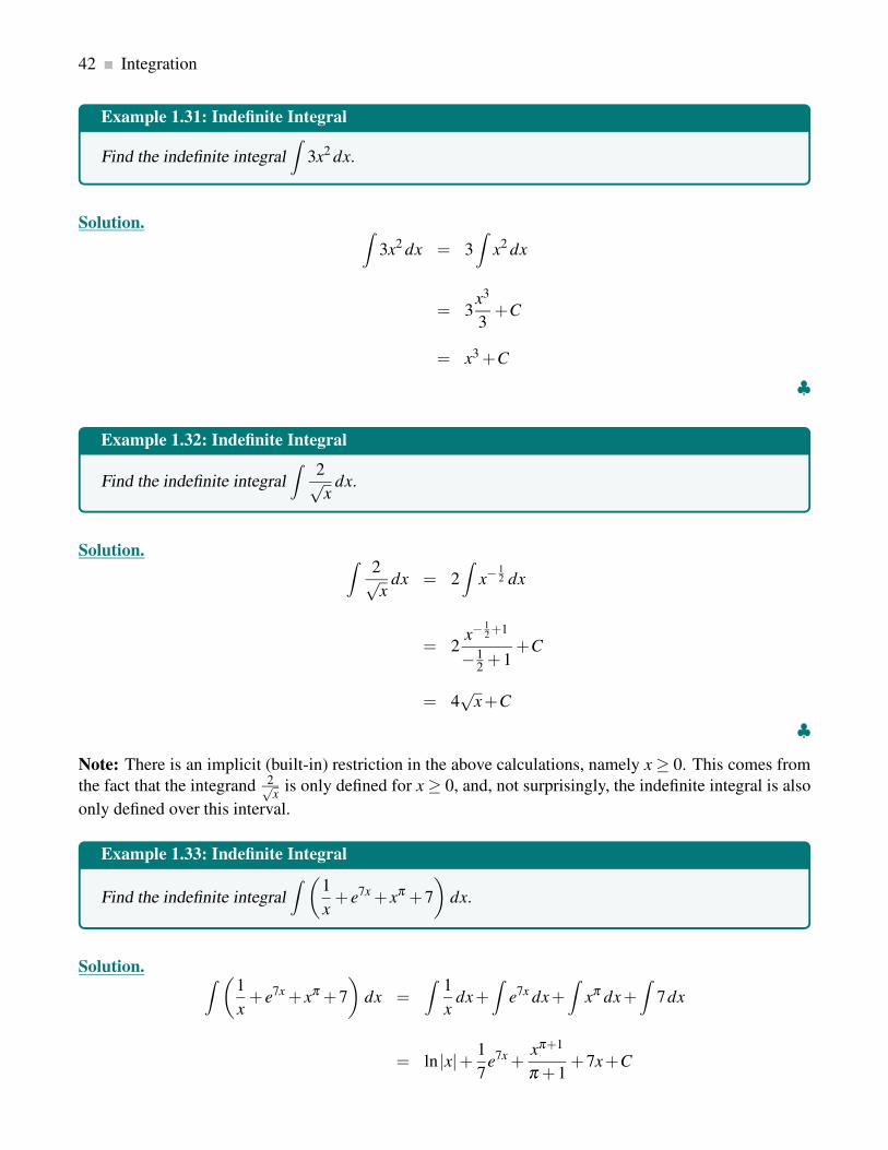
42 Integration
Example 1.31: Indefinite Integral
Find the indefinite integral
∫
3x2 dx.
Solution.∫
3x2 dx = 3
∫
x2 dx
= 3x3
3+C
= x3 +C
♣
Example 1.32: Indefinite Integral
Find the indefinite integral
∫
2√x
dx.
Solution.∫
2√x
dx = 2
∫
x−12 dx
= 2x−
12+1
−12 +1
+C
= 4√
x+C
♣
Note: There is an implicit (built-in) restriction in the above calculations, namely x ≥ 0. This comes from
the fact that the integrand 2√x
is only defined for x ≥ 0, and, not surprisingly, the indefinite integral is also
only defined over this interval.
Example 1.33: Indefinite Integral
Find the indefinite integral
∫
(
1
x+ e7x + xπ +7
)
dx.
Solution.∫
(
1
x+ e7x + xπ +7
)
dx =∫
1
xdx+
∫
e7x dx+∫
xπ dx+∫
7dx
= ln |x|+ 1
7e7x +
xπ+1
π +1+7x+C

1.5. Indefinite Integrals 43
♣
Note: Just like in the previous example, the rule for integration 1x also comes with an implicit restriction,
namely x 6= 0. The function 1x clearly has a well defined area, as long as you stick to values of x < 0 or
x > 0 and is undefined for x = 0, but lnx is undefined for x ≤ 0. However, we know from differential
calculus that ddx ln |x| = 1
x (try this derivative again to convince yourself by rewriting this function as a
peicewise-defined function). Hence, the antiderivative of 1x becomes ln |x|.
Example 1.34: Finding Cost Functions
Suppose a publishing company has found that the marginal cost at a level of production of x thou-
sand magazines is given by
C′(x) =25√
x
and that the fixed cost, i.e. the cost before the first book can be produced, is $36,000. Find the cost
function C(x).
Solution. By the indefinite integral rules
∫
25√x
dx =∫
25x−1/2dx = 25(2x1/2)+ k = 50x1/2 + k,
where k represents the constant of integration to avoid confusion with the cost function. Notice that the
production x is always non-negative, and so we proceed with the integration with the implicit assumption
that x ≥ 0 is automatically satisfied.
To find the value of k, use the fact that C(0) is 36,000.
C(x) = 50x1/2 + k
36,000 = 50 ·0+ k
k = 36,000
With this result, the cost function is C(x) = 50x1/2 +36,000. ♣
Example 1.35: Finding Revenue and Demand Functions
Suppose the marginal revenue from a product is given by
800e−0.2 +7.5.
(a) Find the revenue function for this product.
(b) Find the demand function for this product.
Solution.

44 Integration
(a) The marginal revenue is the derivative of the revenue function, so
R′(q) = 800e−0.2q +7.5
R(q) =∫
(
800e−0.2q +7.5)
dq
= 800e−0.2q
−0.2+7.5q+C
=−4000e−0.2q +7.5q+C
If no items are sold, then there is no revenue. Hence, q = 0 and R = 0, and so
0 =−4000e−0.2(0)+7.5(0)+C
0 =−4000+C
C = 4000
Therefore, the revenue function is
R(q) =−4000e−0.2q +7.5q+4000.
(b) Recall that R = qp, where p is the demand function that represents the price p as a function of q. So
−4000e−0.2q +7.5q+4000 = qp
−4000e−0.2q +7.5q+4000
q= p
Therefore, the demand function is
p(q) =−4000e−0.2q +7.5q+4000
q.
♣
1.5.4. Differential Equations and Constants of Integration
An equation involving derivatives where we want to solve for the original function is called a differential
equation. For example, f ′(x) = 2x is a differential equation with general solution f (x) = x2 +C. Some

1.5. Indefinite Integrals 45
solutions (i.e., particular values of C) are shown below.
As seen with integral curves, we may have an infinite family of solutions satisfying the differential equa-
tion. However, if we were given a point (called an initial value) on the curve then we could determine
f (x) completely. Such a problem is known as an initial value problem.
Example 1.36: Initial Value Problem
If f ′(x) = 2x and f (0) = 2 then determine f (x).
Solution. As previously stated, we have a solution of:
f (x) = x2 +C.
But f (0) = 2 implies:
2 = 02 +C → C = 2.
Therefore, f (x) = x2 +2 is the solution to the initial value problem. ♣
Exercises for Section 1.5
Exercise 1.5.1 Find the following indefinite integrals.
(a)
∫
8√
xdx (b)
∫
3t2+1dt (c)
∫
4/√
ydy

46 Integration
(d)
∫
2/z2dz
(e)
∫
7s−1ds
(f)
∫
(5x+1)2dx
(g)
∫
(t −6)2dt
(h)
∫
z3/2dz
(i)
∫
2
x√
xdx
(j)
∫
|2t −4|dt
(k)
∫
(cos(2x)+4sin(x))dx
(l)
∫
(
2y− sec2 y)
dy
(m)
∫
(
tanx
cosx− csc2 x
)
dx
Exercise 1.5.2 Find the following indefinite integrals. Hint: Simplify the integrand first.
(a)
∫
2s3 + s2 − s
sds
(b)
∫
3x3 − x2 + x−2
xdx
(c)
∫
u3 + 3√
2u
2u2du
(d)
∫
(√t −2
)2
4t2dt
Exercise 1.5.3 Solve the initial value problems to find f (t).
(a) f ′(t) = 3t +2, where f (0) = 5
(b) f ′(t) = t+3t , where f (1) =−1
(c) f ′(t) = sin t, where f (π) = 0
(d) f ′(t) = e2x −4, where f (0) = 1
Exercise 1.5.4 A retailer determines that the marginal revenue function associated with selling q items is
R′(q) =−0.008q+16
dollars per week per item.
(a) Determine R(q).
(b) Determine the demand equation relating the unit price p to the quantity q demanded.
Exercise 1.5.5 A supermarket determines that the marginal profit function associated with purchasing
and selling q heads of lettuce is
P′(q) =−0.003q+15,
dollars per year per unit. Given that the fixed storage cost is $1000 per year, what is the maximum possible
daily profit?
Exercise 1.5.6 The same supermarket determines that the marginal cost of storing q bouquets of flowers
is approximately
C′(q) = 0.001q+50
dollars per week, with a fixed cost of $500 per week. Determine the total monthly cost of storing 500
bouquets a week.

1.5. Indefinite Integrals 47
Exercise 1.5.7 A microbiologist is in charge of counting bacteria in a Petri dish. Starting with a single
bacterium, she determines that the organisms are increasing at a rate of
N′(t) =−2t2 +10t +100
for t ∈ [0,5] hours.
(a) Determine as a function of t the number of organisms in the Petri dish.
(b) Over the entire interval studied, what was the average number of organisms in the dish?

2. Techniques of Integration
Over the next few sections we examine some techniques that are frequently successful when seeking
antiderivatives of functions.
2.1 Substitution Rule
2.1.1. Substitution Rule for Indefinite Integrals
Needless to say, most integration problems we will encounter will not be so simple. That is to say we will
require more than the basic integration rules we have seen. Here’s a slightly more complicated example:
Find∫
2xcos(x2)dx.
This is not a “simple” derivative, but a little thought reveals that it must have come from an application
of the Chain Rule. Multiplied on the “outside” is 2x, which is the derivative of the “inside” function x2.
Checking:d
dxsin(x2) = cos(x2)
d
dxx2 = 2xcos(x2)
so∫
2xcos(x2)dx = sin(x2)+C.
To summarize: If we suspect that a given function is the derivative of another via the Chain Rule, we
let u denote a likely candidate for the inner function, then translate the given function so that it is written
entirely in terms of u, with no x remaining in the expression. If we can integrate this new function of u,
then the antiderivative of the original function is obtained by replacing u by the equivalent expression in
x. This result leads us to the following theorem.
Theorem 2.1: Substitution Rule for Indefinite Integrals
If u = g(x) is a differentiable function whose range is an interval I and f is continuous on I, then
∫
f (g(x))g′(x)dx =∫
f (u)du.
We can describe two methods how the Substitution Rule may unfold in an integration process.
48

2.1. Substitution Rule 49
Method 1: Even in simple cases you may prefer to use this mechanical procedure, since it often helps to
avoid silly mistakes. For example, consider again this simple problem:
∫
2xcos(x2)dx.
Let u = x2, then du/dx = 2x or du = 2xdx. Since we have exactly 2xdx in the original integral, we can
replace it by du:∫
2xcos(x2)dx =
∫
cosudu = sinu+C = sin(x2)+C.
Method 2: This is not the only way to do the algebra, and typically there are many paths to the correct
answer. For example, since du/dx = 2x, we have that dx = du/2x, and so the integral becomes
∫
2xcos(x2)dx =
∫
2xcosudu
2x=
∫
cosudu.
Guideline for Substitution Rule
Given the integral
I =∫
f (g(x))g′(x)dx
with f continuous and g differentiable, the following steps outline the Substitution Rule process
for integrating I.
1. Let u = g(x), which is typically the inside function of the function composition in the inte-
grand.
2. Compute du = g′(x)dx.
3. Write the integral I solely in terms of u using either method:
(a) use the substitution u = g(x) and du = g′(x)dx; or
(b) replace dx with du/g′(x) and cancel g′(x).
4. Integrate with respect to u.
5. Replace u by g(x) to write the result in terms of x only.
Note:
1. However the Substitution Rule unfolds in the solution process, the important part is that you must
eliminate all instances of the original variable, often x, during the process and then write your result
back in terms of the original variable x.
2. Sometimes, the integrand has to be rearranged to see whether the Substitution Rule is a possible
integration technique.
3. If a first substitution did not work out, then try to simplify or rearrange the integrand to see if a
different substitution can be used.

50 Techniques of Integration
4. As a general guideline for the Substitution Rule, we look for the inside function u to be
• the radicand under a root: e.g.,
when
∫
x3√
x2 −5dx we choose u = x2 −5;
• the base in a power with a real exponent: e.g.,
when
∫
x(
x2 −5)5
dx we choose u = x2 −5;
• the exponent in a power with a real base: e.g.,
when
∫
x5x2−5 dx we choose u = x2 −5;
• the denominator in a fraction: e.g.,
when
∫
x
x2 −5dx we choose u = x2 −5.
However, sometimes u can be something different than is suggested above, so be open minded about
this process.
Example 2.2: Substitution Rule
Evaluate
∫
(ax+b)n dx, assuming a,b are constants, a 6= 0, and n is a positive integer.
Solution. We let u = ax+b so du = adx or dx = du/a. Then
∫
(ax+b)n dx =
∫
1
aun du =
1
a(n+1)un+1 +C =
1
a(n+1)(ax+b)n+1 +C.
♣
Example 2.3: Substitution Rule
Evaluate
∫
sin(ax+b)dx, assuming that a and b are constants and a 6= 0.
Solution. Again we let u = ax+b so du = adx or dx = du/a. Then
∫
sin(ax+b)dx =
∫
1
asinudu =
1
a(−cosu)+C =−1
acos(ax+b)+C.
♣

2.1. Substitution Rule 51
Example 2.4: Substitution in Denominator
Evaluate the following integral:
∫
2y√
1−4y2dy.
Solution. We try the substitution:
u = 1−4y2.
Then,
du =−8y dy
In the numerator we have 2y dy, so rewriting the differential gives:
−1
4du = 2y dy.
Then the integral is:
∫
2y√
1−4y2dy =
∫
(
1−4y2)−1/2
(2y dy)
=∫
u−1/2
(
−1
4du
)
=
(−1
4
)
u1/2
1/2+C
= −√
1−4y2
2+C
♣
Example 2.5: Substitution in Base
Evaluate the following integral:
∫
cosx(sinx)5 dx.
Solution. In this question we will let u = sinx. Then,
du = cosx dx.
Thus, the integral becomes:
∫
cosx(sinx)5 dx =
∫
u5 du
=u6
6+C
=(sinx)6
6+C

52 Techniques of Integration
♣
Example 2.6: Substitution
Evaluate the following integral:
∫
cos(√
x)√x
dx.
Solution. We use the substitution:
u = x1/2.
Then,
du =1
2x−1/2 dx.
Rewriting the differential we get:
2 du =1√x
dx.
The integral becomes:
∫
cos(√
x)√x
dx = 2
∫
cosudu
= 2sinu+C
= 2sin(√
x)+C
♣
Example 2.7: Substitution
Evaluate the following integral:
∫
2x3√
x2 +1dx.
Solution. This problem is a little bit different than the previous ones. It makes sense to let:
u = x2 +1,
then
du = 2x dx.
Making this substitution gives:
∫
2x3√
x2 +1dx =
∫
x2√
x2 +1(2x)dx
=∫
x2u1/2 du

2.1. Substitution Rule 53
This is a problem because our integrals can’t have a mixture of two variables in them. Usually this means
we chose our u incorrectly. However, in this case we can eliminate the remaining x’s from our integral by
using:
u = x2 +1 =⇒ x2 = u−1.
We get:
∫
x2u1/2 du =∫
(u−1)u1/2 du.
Now we proceed by simplifying the integrand and noticing we are left with power functions, which are
readily integrated.∫
(u−1)u1/2 du =
∫
u3/2 −u1/2 du =2
5u5/2 − 2
3u3/2 +C.
Therefore, our original integral becomes∫
2x3√
x2 +1dx =2
5(x2 +1)5/2 − 2
3(x2 +1)3/2 +C
♣
Example 2.8: Two Choices for Substitution
Evaluate
∫
2x3√
x2 −5dx.
Solution.
Method 1: Let u = x2 −5, du = 2xdx.∫
2x3√
x2 −5dx =
∫
du
u1/3
=u2/3
2/3+C
=3
2u2/3 +C
=3
2
(
x2 −5)2/3
+C
Method 2: Let u =3√
x2 −5, u3 = x2 −5, 3u2du = 2xdx.∫
2x3√
x2 −5dx =
∫
3u2du
u
= 3
∫
udu
= 3u2
2+C
=3
2
(
x2 −5)2/3
+C

54 Techniques of Integration
♣
Example 2.9: Application in Sales Projection
An airline wants to predict the number of tickets on a particular route that will be sold. They find
that over the next year, ticket sales growth after t weeks can be modelled by
1000−500e−0.025t
tickets per week for t ∈ [0,52].
(a) Determine the predicted total number of tickets sold after the first t weeks.
(b) Determine the predicted total number of tickets sold in the next year.
Solution.
(a) Let N(t) be the total number of tickets predicted to be sold after the first t months. We are given
N′(t) = 1000−500e−0.025t .
Thus,
N(t) =∫
(
1000−500e−0.025t)
dt.
We integrate by substitution. Let u =−0.025t, du =−0.025dt:
N(t) =
∫
(
1000−500e−0.025t)
dt
=
∫
1000dt +500
0.025
∫
eu du
= 1000t +20,000e−0.025t +C
It remains to determine the value of C. We require
N(0) = 0 =⇒ C =−20,000.
Therefore, the total number of tickets sold after the first t months is predicted to be
N(t) = 1000t +20,000e−0.025t −20,000.
(b) Since
N(52) = 1000(52)+20,000e−0.025(52)−20,000 = 37450.64,
we have that the model predicts that 37,451 tickets will be sold on this route in the next year.
♣

2.1. Substitution Rule 55
2.1.2. Substitution Rule for Definite Integrals
The next example shows how to use the Substitution Rule when dealing with definite integrals.
Example 2.10: Substitution Rule with Two Methods
Evaluate
∫ 4
2xsin(x2)dx.
Solution.
Method 1: First Compute the Antiderivative, then Evaluate the Definite Integral.
Let u = x2, so du = 2xdx or xdx = du/2. Then
∫
xsin(x2)dx =∫
1
2sinudu =
1
2(−cosu)+C =−1
2cos(x2)+C.
Now∫ 4
2xsin(x2)dx = −1
2cos(x2)
∣
∣
∣
∣
4
2
=−1
2cos(16)+
1
2cos(4).
Method 2: Changing the Limits of Integration with the Substitution.
A somewhat neater alternative to this method is to change the original limits to match the variable u. Since
u = x2, when x = 2, u = 4, and when x = 4, u = 16. So we can do this:
∫ 4
2xsin(x2)dx =
∫ 16
4
1
2sinudu = −1
2(cosu)
∣
∣
∣
∣
16
4
=−1
2cos(16)+
1
2cos(4).
An incorrect, and dangerous, alternative is something like this:
∫ 4
2xsin(x2)dx =
∫ 4
2
1
2sinudu = −1
2cos(u)
∣
∣
∣
∣
4
2
= −1
2cos(x2)
∣
∣
∣
∣
4
2
=−1
2cos(16)+
1
2cos(4).
This is incorrect because
∫ 4
2
1
2sinudu means that u takes on values between 2 and 4, which is wrong. It
is dangerous, because it is very easy to get to the point −1
2cos(u)
∣
∣
∣
∣
4
2
and forget to substitute x2 back in for
u, thus getting the incorrect answer −1
2cos(4)+
1
2cos(2). An acceptable alternative is to clearly indicate
that the limit substitution is to be done with respect to the x variable, using something like:
∫ 4
2xsin(x2)dx =
∫ x=4
x=2
1
2sinudu = −1
2cos(u)
∣
∣
∣
∣
x=4
x=2
= −1
2cos(x2)
∣
∣
∣
∣
4
2
=−cos(16)
2+
cos(4)
2.
♣
To summarize, we have the following.

56 Techniques of Integration
Theorem 2.11: Substitution Rule for Definite Integrals
If g′ is continuous on [a,b] and f is continuous on the range of u = g(x), then
∫ b
af (g(x))g′(x)dx =
∫ g(b)
g(a)f (u)du.
Note: When using the Substitution Rule when integrating definite integrals, it is important to change the
limits of integration from those of the original function to those of the substituted function. Otherwise, the
definite integral will evaluate to an incorrect result.
Example 2.12: Substitution Rule for Definite Integrals
Evaluate
∫ 1/2
1/4
cos(πt)
sin2(πt)dt.
Solution. Let u = sin(πt) so du = π cos(πt)dt or du/π = cos(πt)dt. We change the limits to u(1/4) =
sin(π/4) =√
2/2 and u(1/2) = sin(π/2) = 1. Then
∫ 1/2
1/4
cos(πt)
sin2(πt)dt =
∫ 1
√2/2
1
π
1
u2du =
∫ 1
√2/2
1
πu−2 du =
1
π
u−1
−1
∣
∣
∣
∣
1
√2/2
=− 1
π+
√2
π.
♣
Example 2.13: Substitution Rule for Definite Integrals
Evaluate
∫ 1
−1(y+1)
(
y2 +2y)8
dy.
Solution. Although we could expand the integrand, since this would yield powers of y which we can
certainly integrate without using the Substitution Rule at all, the exponent 8 would make this a rather
messy process that is surely prone to errors. Instead we proceed with the obvious choice of substitution
and let u = y2 +2y, then
dy = (2y+2)dy = 2(y+1)dy =⇒ du
2= (y+1)dy
with limits of integration
u(−1) = (−1)2 +2(−1) =−1 and u(1) = (1)2+2(1) = 3.
Take note that sometimes the value of a limit of integration does not change. The point is that one still
needs to substitute the values of the original variable of integration, in this case y, to work with the limits
of integration for the substituted variable, in this case u.

2.1. Substitution Rule 57
Then the integral evaluates as follows
∫ 1
−1(y+1)
(
y2 +2y)8
dy =
∫ 3
−1
u8
2du =
u9
18
∣
∣
∣
∣
3
−1
=39
18− (−1)9
18=
19,684
18.
♣
Exercises for Section 2.1
Exercise 2.1.1 Evaluate the following indefinite integrals.
(a)
∫
(1− t)9 dt
(b)
∫
(x2 +1)2 dx
(c)
∫
x(x2 +1)100 dx
(d)
∫
13√
1−5tdt
(e)
∫
sin3 xcosxdx
(f)
∫
x√
100− x2 dx
(g)
∫
x2
√1− x3
dx
(h)
∫
cos(πt)cos(
sin(πt))
dt
(i)
∫
sinx
cos3 xdx
(j)
∫
tanxdx
(k)
∫
sec2 x tanxdx
(l)
∫
sin(tanx)
cos2 xdx
(m)
∫
6x
(x2 −7)1/9dx
(n)
∫
f (x) f ′(x)dx
Exercise 2.1.2 Evaluate the following definite integrals.
(a)
∫ π
0sin5(3x)cos(3x)dx
(b)
∫
√π/2
0xsec2(x2) tan(x2)dx
(c)
∫ 4
3
1
(3x−7)2dx
(d)
∫ π/6
0(cos2 x− sin2 x)dx
(e)
∫ 1
−1(2x3 −1)(x4 −2x)6 dx
(f)
∫ 1
−1sin7 xdx
Exercise 2.1.3 A toy truck manufacturer estimates that the number of sales after Christmas declines at a
rate of
−3e−0.2t
toys per day (t ∈ [0,60]). If the manufacturer sells 10,000 units on Christmas day (t = 0), determine the
number of expected sales after t days.
Exercise 2.1.4 Let q be the quantity (in thousands) of a product in the market when the unit price is
set at p dollars per unit. There are currently 2000 units available at a price of $2/unit. Determine the

58 Techniques of Integration
corresponding supply equation if the price increases at a rate of
p′(q) =100q
(1−q)2.
Exercise 2.1.5 Let q represent the daily quantity demanded (in thousands) of a certain product. When the
unit price p is set at $3, it is observed that 1000 units are demanded per day. Determine the corresponding
demand equation if the price decreases at a rate of
p′(q) =−200q
(3+q2)3/2.
Exercise 2.1.6 In the first month (t = 0) following a successful marketing campaign, a company sells
2,000 units of their product. Management predicts that the sales will decline at a rate of
N′(t) =−200(e−2t +1)
units per month for the next 3 months. Determine the total number of expected sales after 3 months.
2.2 Powers of Trigonometric Functions
The trigonometric substitutions we will focus on in this section are summarized in the table below:
Substitution u = sinx u = cosx u = tanx u = secx
Derivative du = cosxdx du =−sinxdx du = sec2 xdx du = secx tanxdx
2.2.1. Products of Powers of Sine and Cosine
Functions consisting of powers of the sine and cosine can be integrated by using substitution and trigono-
metric identities. These can sometimes be tedious, but the technique is straightforward. A similar tech-
nique is applicable to powers of secant and tangent as shown in Section 2.2.2 (and also cosecant and
cotangent, not discussed here). An example will suffice to explain the approach.
Example 2.14: Odd Power of Sine
Evaluate
∫
sin5 xdx.
Solution. Rewrite the function:∫
sin5 xdx =∫
sinxsin4 xdx

2.2. Powers of Trigonometric Functions 59
=∫
sinx(sin2 x)2 dx
=
∫
sinx(1− cos2 x)2 dx.
Now use u = cosx, du =−sinxdx:∫
sinx(1− cos2 x)2 dx =
∫
−(1−u2)2 du
=
∫
−(1−2u2+u4)du
=∫
1+2u2−u4 du
= −u+2
3u3 − 1
5u5 +C
= −cosx+2
3cos3 x− 1
5cos5 x+C. ♣
Observe that by taking the substitution u = cosx in the last example, we ended up with an even power
of sine from which we can use the formula sin2 x+ cos2 x = 1 to replace any remaining sines. We then
ended up with a polynomial in u in which we could expand and integrate quite easily. Notice here that the
“obvious” substitution u = sinx in the original integral does not lead to any useful simplification.
This technique works for products of powers of sine and cosine. We summarize it below.
Guideline for Integrating Products of Sine and Cosine
When evaluating
∫
sinm xcosn xdx:
1. The power of sine is odd (m odd):
(a) Use u = cosx and du =−sinxdx.
(b) Replace dx using (a), thus cancelling one power of sinx by the substitution of du, and
be left with an even number of sine powers.
(c) Use sin2 x = 1− cos2 x (= 1−u2) to replace the leftover sines.
2. The power of cosine is odd (n odd):
(a) Use u = sinx and du = cosxdx.
(b) Replace dx using (a), thus cancelling one power of cosx by the substitution of du, and
be left with an even number of cosine powers.
(c) Use cos2 x = 1− sin2 x (= 1−u2) to replace the leftover cosines.
3. Both m and n are odd:
Use either 1 or 2 (both will work).
4. Both m and n are even:
Use cos2 x = 12 (1+ cos(2x)) and/or sin2 x = 1
2 (1− cos(2x)) to reduce to a form that can be
integrated.

60 Techniques of Integration
Note: As m and n get large, multiple steps will be needed.
Example 2.15: Odd Power of Cosine and Even Power of Sine
Evaluate
∫
sin6 xcos5 xdx.
Solution. We will show this solution in two ways.
Method 1: We rewrite the integrand to use the Substitution Rule.
∫
sin6 xcos5 xdx =∫
sin6 xcos4 xcosxdx
=
∫
sin6 x(cos2 x)2 cosxdx
=∫
sin6 x(1− sin2 x)2 cosxdx
Then use the substitution u = sinx since the derivative of sinx is cosx, and also because there is only
one occurrence of cosine in the integrand. Hence, du = cosxdx is the perfect substitution.
∫
sin6 x(1− sin2 x)2 cosxdx =∫
u6(1−u2)2du
=
∫
u6 −2u8 +u10 du
=u7
7− 2u9
9+
u11
11+C
=sin7 x
7− 2sin9 x
9+
sin11 x
11+C
Method 2: We apply the Guideline for Integrating Products of Sine and Cosine. Since the power of cosine
is odd, we use the substitution u = sinx and du = cosx.
Then∫
sin6 xcos5 xdx =
∫
u6 cos5 xdu
cosxUsing the substitution
=∫
u6(
cos2 x)2
du Canceling a cosx and rewriting cos4 x
=
∫
u6(1− sin2 x)2 du Using trig identity cos2 x = 1− sin2 x
=∫
u6(1−u2)2 du Writing integral in terms of u’s
=∫
u6 −2u8 +u10 du Expand and collect like terms
=u7
7− 2u9
9+
u11
11+C Integrating
=sin7 x
7− 2sin9 x
9+
sin11 x
11+C Replacing u back in terms of x

2.2. Powers of Trigonometric Functions 61
♣
Example 2.16: Odd Power of Cosine
Evaluate
∫
cos3 xdx.
Solution. Since the power of cosine is odd, we use the substitution u = sinx and du = cosxdx. This may
seem strange at first since we don’t have sinx in the question, but it does work!
∫
cos3 xdx =∫
cos3 xdu
cosxUsing the substitution
=
∫
cos2 xdu Canceling a cosx
=
∫
(1− sin2 x)du Using trig identity cos2 x = 1− sin2 x
=
∫
(1−u2)du Writing integral in terms of u’s
= u− u3
3+C Integrating
= sinx− sin3 x
3+C Replacing u back in terms of x
♣
Example 2.17: Product of Even Powers of Sine and Cosine
Evaluate
∫
sin2 xcos2 xdx.
Solution. Use the formulas
sin2 x =1− cos(2x)
2and cos2 x =
1+ cos(2x)
2
to get∫
sin2 xcos2 xdx =∫
1− cos(2x)
2· 1+ cos(2x)
2dx.
We then have∫
sin2 xcos2 xdx =
∫
1− cos(2x)
2· 1+ cos(2x)
2dx
=1
4
∫
1− cos2 2xdx
=1
4
(
x−∫
cos2 2xdx
)
.
To continue the integration, we use the cosine double angle identity again with
cos2(2x) =1+ cos(4x)
2.

62 Techniques of Integration
Then∫
sin2 xcos2 xdx =1
4
(
x− 1
2
∫
1+ cos4xdx
)
=1
4
(
x− 1
2
(
x+sin4x
4
))
=1
4
(
x− x
2− sin4x
8
)
+C
♣
Example 2.18: Even Power of Sine
Evaluate
∫
sin6 xdx.
Solution. Use sin2 x = (1− cos(2x))/2 to rewrite the function:∫
sin6 xdx =
∫
(sin2 x)3 dx
=∫
(1− cos2x)3
8dx
=1
8
∫
1−3cos2x+3cos2 2x− cos3 2xdx.
Now we have four integrals to evaluate. Ignoring the constant for now:∫
1dx = x
and∫
−3cos2xdx =−3
2sin2x
are easy. The cos3 2x integral is like the previous example:∫
−cos3 2xdx =
∫
−cos2xcos2 2xdx
=∫
−cos2x(1− sin2 2x)dx
=
∫
−1
2(1−u2)du
= −1
2
(
u− u3
3
)
= −1
2
(
sin2x− sin3 2x
3
)
.
And finally we use another trigonometric identity, cos2 x = (1+ cos(2x))/2:
∫
3cos2 2xdx = 3
∫
1+ cos4x
2dx =
3
2
(
x+sin4x
4
)
.
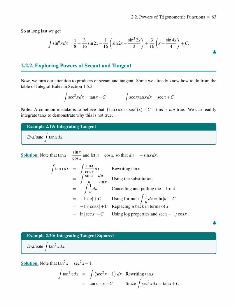
2.2. Powers of Trigonometric Functions 63
So at long last we get
∫
sin6 xdx =x
8− 3
16sin2x− 1
16
(
sin2x− sin3 2x
3
)
+3
16
(
x+sin4x
4
)
+C.
♣
2.2.2. Exploring Powers of Secant and Tangent
Now, we turn our attention to products of secant and tangent. Some we already know how to do from the
table of Integral Rules in Section 1.5.3.∫
sec2 xdx = tanx+C
∫
secx tanxdx = secx+C
Note: A common mistake is to believe that∫
tanxdx is sec2(x)+C – this is not true. We can readily
integrate tanx to demonstrate why this is not true.
Example 2.19: Integrating Tangent
Evaluate
∫
tanxdx.
Solution. Note that tanx =sinx
cosxand let u = cosx, so that du =−sinxdx.
∫
tanxdx =∫
sinx
cosxdx Rewriting tanx
=
∫
sinx
u
du
−sinxUsing the substitution
= −∫
1
udu Cancelling and pulling the −1 out
= − ln |u|+C Using formula
∫
1
udx = ln |u|+C
= − ln |cosx|+C Replacing u back in terms of x
= ln |secx|+C Using log properties and secx = 1/cosx
♣
Example 2.20: Integrating Tangent Squared
Evaluate
∫
tan2 xdx.
Solution. Note that tan2 x = sec2 x−1.∫
tan2 xdx =
∫
(
sec2 x−1)
dx Rewriting tanx
= tanx− x+C Since
∫
sec2 xdx = tanx+C

64 Techniques of Integration
♣
Note: In problems with tangent and secant, two integrals come up frequently:
∫
sec3 xdx and
∫
secxdx.
Both have relatively nice expressions but they are a bit tricky to discover.
First we evaluate
∫
secxdx, which we will need to compute
∫
sec3 xdx.
Example 2.21: Integral of Secant
Evaluate
∫
secxdx.
Solution. We start with a trick, namely we multiply the integrand by 1, but we express 1 as the ratio
(secx+ tanx)/(secx+ tanx). This sounds like a crazy idea, but it works!
∫
secxdx =
∫
secxsecx+ tanx
secx+ tanxdx
=∫
sec2 x+ secx tanx
secx+ tanxdx.
Now let u = secx+ tanx, du = secx tanx+sec2 xdx, exactly the numerator of the function we are integrat-
ing. Thus
∫
secxdx =
∫
sec2 x+ secx tanx
secx+ tanxdx
=∫
1
udu = ln |u|+C
= ln |secx+ tanx|+C.
♣
Now we compute the integral
∫
sec3 xdx.
Example 2.22: Integral of Secant Cubed
Evaluate
∫
sec3 xdx.
Solution.
sec3 x =sec3 x
2+
sec3 x
2=
sec3 x
2+
(tan2 x+1)secx
2

2.2. Powers of Trigonometric Functions 65
=sec3 x
2+
secx tan2 x
2+
secx
2
=sec3 x+ secx tan2 x
2+
secx
2.
We already know how to integrate secx, so we just need the first quotient. This is “simply” a matter of
recognizing the Product Rule differentiation in action:
∫
sec3 x+ secx tan2 xdx = secx tanx.
So putting these together we get
∫
sec3 xdx =secx tanx
2+
ln |secx+ tanx|2
+C,
♣
2.2.3. Products of Powers of Secant and Tangent
For products of secant and tangent it is best to use the following Guideline.
Guideline for Integrating Products of Secant and Tangent
When evaluating
∫
secm x tann xdx:
1. The power of secant is even (m even):
(a) Use u = tanx and du = sec2 xdx.
(b) Cancel sec2 x by the substitution of dx, and be left with an even number of secants.
(c) Use sec2 x = 1+ tan2 x (= 1+u2) to replace the leftover secants.
2. The power of tangent is odd (n odd):
(a) Use u = secx and du = secx tanxdx.
(b) Cancel one secx and one tanx by the substitution of dx. The number of remaining
tangents is even.
(c) Use tan2 x = sec2 x−1 (= u2 −1) to replace the leftover tangents.
3. m is even or n is odd:
Use either 1 or 2 (both will work).
4. The power of secant is odd and the power of tangent is even:
No guideline. The integrals
∫
secxdx and
∫
sec3 xdx can usually be looked up, or recalled
from memory.

66 Techniques of Integration
Example 2.23: Even Power of Secant
Evaluate
∫
sec6 x tan6 xdx.
Solution. Since the power of secant is even, we use u = tanx, so that du = sec2 xdx.
∫
sec6 x tan6 xdx =
∫
sec6 x(u6)du
sec2 xUsing the substitution
=
∫
sec4 x(u6)du Cancelling a sec2 x
=
∫
(sec2 x)2(u6)du Rewriting sec4 x
=∫
(1+ tan2 x)2(u6)du Using sec2 x = 1+ tan2 x
=∫
(1+u2)2(u6)du Using the substitution
To integrate this product the easiest method is expand it into a polynomial and integrate term-by-term.
∫
sec6 x tan6 xdx =∫
(u6+2u8 +u10)du Expanding
=u7
7+
2u9
9+
u11
11+C Integrating
=tan7 x
7+
2tan9 x
9+
tan11 x
11+C Rewriting in terms of x
♣
Example 2.24: Odd Power of Tangent
Evaluate
∫
sec5 x tanxdx.
Solution. Since the power of tangent is odd, we use u = secx, so that du = secx tanxdx. Then we have:
∫
sec5 x tanxdx =∫
sec5 x tanxdu
secx tanxSubstituting dx first
=∫
sec4 xdu Cancelling
=∫
u4 du Using the substitution
=u5
5+C Integrating
=sec5 x
5+C Rewriting in terms of x

2.2. Powers of Trigonometric Functions 67
♣
Example 2.25: Odd Power of Secant and Even Power of Tangent
Evaluate
∫
secx tan2 xdx.
Solution. The Guideline doesn’t help us in this scenario. However, since tan2 x = sec2 x−1, we have
∫
secx tan2 xdx =∫
secx(sec2 x−1)dx
=∫
(sec3 x− secx)dx
=1
2(secx tanx+ ln |secx+ tanx|)− ln |secx+ tanx|+C
=1
2secx tanx+
1
2ln |secx+ tanx|− ln |secx+ tanx|+C
=1
2secx tanx− 1
2ln |secx+ tanx|+C
♣
Exercises for Section 2.2
Exercise 2.2.1 Evaluate the following indefinite integrals.
(a)
∫
sin2 xdx
(b)
∫
sin3 xdx
(c)
∫
sin4 xdx
(d)
∫
cos2 xsin3 xdx
(e)
∫
cos3 xdx
(f)
∫
cos3 xsin2 xdx
(g)
∫
sinx(cosx)3/2 dx
(h)
∫
sec2 xcsc2 xdx
(i)
∫
tan3 xsecxdx
(j)
∫
(
1
cscx+
1
secx
)
dx
(k)
∫
cos2 x+ cosx+1
cos3 xdx
(l)
∫
xsec2(x2) tan4(x2)dx
(m)
∫
xsec2(x2) tan4(x2)dx

68 Techniques of Integration
2.3 Trigonometric Substitutions
So far we have seen that it sometimes helps to replace a subexpression of a function by a single variable.
Occasionally it can help to replace the original variable by something more complicated. This seems like
a “reverse” substitution, but it is really no different in principle than ordinary substitution.
Example 2.26: Sine Substitution
Evaluate
∫
√
1− x2 dx.
Solution. Let x = sinu so dx = cosudu. Then∫
√
1− x2 dx =
∫
√
1− sin2 ucosudu =
∫ √cos2 ucosudu.
We would like to replace√
cos2 u by cosu, but this is valid only if cosu is positive, since√
cos2 u is
positive. Consider again the substitution x = sinu. We could just as well think of this as u = arcsinx. If we
do, then by the definition of the arcsine, −π/2 ≤ u ≤ π/2, so cosu ≥ 0 and so we are allowed to continue
and perform the simplification:∫ √
cos2 ucosudu =∫
cos2 udu
=
∫
1+ cos2u
2du =
u
2+
sin2u
4+C
=arcsinx
2+
sin(2arcsinx)
4+C.
This is a perfectly good answer, though the term sin(2arcsinx) is a bit unpleasant. It is possible to simplify
this. Using the identity sin2x= 2sinxcosx, we can write sin2u= 2sinucosu= 2sin(arcsinx)√
1− sin2 u=
2x
√
1− sin2(arcsinx) = 2x√
1− x2. Then the full antiderivative is
arcsinx
2+
2x√
1− x2
4+C =
arcsinx
2+
x√
1− x2
2+C.
♣
Note:
1. This type of substitution is usually indicated when the function you wish to integrate contains a
polynomial expression that might allow you to use the fundamental identity sin2 x+ cos2 x = 1 in
one of three forms:
cos2 x = 1− sin2 x sec2 x = 1+ tan2 x tan2 x = sec2 x−1.
If your function contains 1− x2, as in the example above, try x = sinu; if it contains 1+ x2 try
x = tanu; and if it contains x2 − 1, try x = secu. Sometimes you will need to try something a bit
different to handle constants other than inverse substitution, which is described next.

2.3. Trigonometric Substitutions 69
2. In a traditional substitution we let u = u(x), i.e., our new variable is defined in terms of x. In an
inverse substitution we let x = g(u), i.e., we assume x can be written in terms of u. We cannot do
this arbitrarily since we do NOT get to “choose” x. For example, an inverse substitution of x = 1
will give an obviously wrong answer. However, when x = g(u) is an invertible function, then we are
really doing a u-substitution with u = g−1(x). Now the Substitution Rule applies.
3. Sometimes with inverse substitutions involving trig functions we use θ instead of u. Thus, we would
take x = sinθ instead of x = sinu.
4. We would like our inverse substitution x = g(u) to be a one-to-one function, and x = sinu is not
one-to-one. In the next few paragraphs, we discuss how we can overcome this issue by using the
restricted trigonometric functions.
The three common trigonometric substitutions are the restricted sine, restricted tangent and restricted
secant. Thus, for sine we use the domain [−π/2, π/2] and for tangent we use (−π/2, π/2). Depending
on the convention chosen, the restricted secant function is usually defined in one of two ways.
One convention is to restrict secant to the region [0, π/2)∪ (π/2,π ] as shown in the middle graph.
The other convention is to use [0, π/2)∪ [π , 3π/2) as shown in the right graph. Both choices give a
one-to-one restricted secant function and no universal convention has been adopted. To make the analysis
in this section less cumbersome, we will use the domain [0, π/2)∪ [π , 3π/2) for the restricted secant
function. Then sec−1 x is defined to be the inverse of this restricted secant function.
Typically trigonometric substitutions are used for problems that involve radical expressions. The table
below outlines when each substitution is typically used along with their restricted intervals.
Expression Substitution Restricted Interval
√a2 − x2 x = asinθ θ ∈ [−π/2, π/2]
√a2 + x2 or a2 + x2 x = a tanθ θ ∈ (−π/2, π/2)
√x2 −a2 x = asecθ θ ∈ [0, π/2)∪ [π , 3π/2)
All three substitutions are one-to-one on the listed intervals. When dealing with radicals we often end up
with absolute values since√
z2 = |z|.
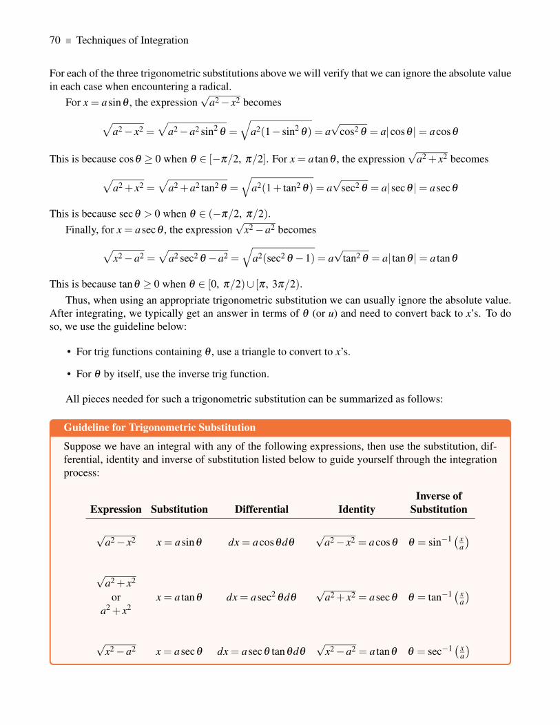
70 Techniques of Integration
For each of the three trigonometric substitutions above we will verify that we can ignore the absolute value
in each case when encountering a radical.
For x = asinθ , the expression√
a2 − x2 becomes
√
a2 − x2 =√
a2 −a2 sin2 θ =
√
a2(1− sin2 θ) = a√
cos2 θ = a|cosθ |= acosθ
This is because cosθ ≥ 0 when θ ∈ [−π/2, π/2]. For x = a tanθ , the expression√
a2 + x2 becomes
√
a2 + x2 =√
a2 +a2 tan2 θ =√
a2(1+ tan2 θ) = a√
sec2 θ = a|secθ |= asecθ
This is because secθ > 0 when θ ∈ (−π/2, π/2).
Finally, for x = asecθ , the expression√
x2 −a2 becomes
√
x2 −a2 =√
a2 sec2 θ −a2 =√
a2(sec2 θ −1) = a√
tan2 θ = a| tanθ |= a tanθ
This is because tanθ ≥ 0 when θ ∈ [0, π/2)∪ [π , 3π/2).
Thus, when using an appropriate trigonometric substitution we can usually ignore the absolute value.
After integrating, we typically get an answer in terms of θ (or u) and need to convert back to x’s. To do
so, we use the guideline below:
• For trig functions containing θ , use a triangle to convert to x’s.
• For θ by itself, use the inverse trig function.
All pieces needed for such a trigonometric substitution can be summarized as follows:
Guideline for Trigonometric Substitution
Suppose we have an integral with any of the following expressions, then use the substitution, dif-
ferential, identity and inverse of substitution listed below to guide yourself through the integration
process:
Inverse of
Expression Substitution Differential Identity Substitution
√a2 − x2 x = asinθ dx = acosθdθ
√a2 − x2 = acosθ θ = sin−1
(
xa
)
√a2 + x2
or x = a tanθ dx = asec2 θdθ√
a2 + x2 = asecθ θ = tan−1(
xa
)
a2 + x2
√x2 −a2 x = asecθ dx = asecθ tanθdθ
√x2 −a2 = a tanθ θ = sec−1
(
xa
)

2.3. Trigonometric Substitutions 71
To emphasize the technique, we redo the computation for
∫
√
1− x2 dx.
Example 2.27: Sine Substitution
Evaluate
∫
√
1− x2 dx.
Solution. Since√
1− x2 appears in the integrand we try the trigonometric substitution x = sinθ . (Here we
are using the restricted sine function with θ ∈ [−π/2, π/2] but typically omit this detail when writing out
the solution.) Then dx = cosθ dθ .∫
√
1− x2 dx =
∫
√
1− sin2 θ cosθ dθ Using our (inverse) substitution
=∫ √
cos2 θ cosθ dθ Since sin2 θ + cos2 θ = 1
=∫
|cosθ | · cosθ dθ Since√
cos2 θ = |cosθ |
=∫
cos2 θ dθ Since for θ ∈ [−π2 , π
2 ] we have cosθ ≥ 0.
Often we omit the step containing the absolute value by our discussion above. Now, to integrate a power
of cosine we use the guideline for products of sine and cosine and make use of the identity
cos2 θ =1
2(1+ cos(2θ)).
Our integral then becomes
∫
√
1− x2 dx =1
2
∫
(1+ cos(2θ))dθ =θ
2+
sin(2θ)
4+C
To write the answer back in terms of x we use a right triangle. Since sinθ = x/1 we have the triangle:
The triangle gives sinθ , cosθ , tanθ , but have a sin(2θ). Thus, we use an identity to write
sin(2θ) = 2sinθ cosθ = 2(x
1
)
(√1− x2
1
)
For θ by itself we use θ = sin−1 x. Thus, the integral is
∫
√
1− x2 dx =sin−1 x
2+
x√
1− x2
2+C

72 Techniques of Integration
♣
Example 2.28: Secant Substitution
Evaluate
∫
√25x2 −4
xdx.
Solution. We do not have√
x2 −a2 because of the 25, but if we factor 25 out we get:
∫
√
25(x2 − (4/25))
xdx =
∫
5
√
x2 − (4/25)
xdx.
Now, a = 2/5, so let x = 25 secθ . Alternatively, we can think of the integral as being:
∫
√
(5x)2 −4
xdx
Then we could let u = 5x followed by u = 2secθ , etc. Or equivalently, we can avoid a u-substitution by
letting 5x = 2secθ . In either case we are using the trigonometric substitution x = 25 secθ , but do use the
method that makes the most sense to you! As x = 25 secθ we have dx = 2
5 secθ tanθ dθ .
∫
√25x2 −4
xdx =
∫
√
254sec2 θ25 −4
25 secθ
2
5secθ tanθ dθ Using the substitution
=∫ √
4(sec2 θ −1) · tanθ dθ Cancelling
= 2
∫ √tan2 θ · tanθ dθ Using tan2 θ +1 = sec2 θ
= 2
∫
tan2 θ dθ Simplifying
= 2
∫
(sec2 θ −1)dθ Using tan2 θ +1 = sec2 θ
= 2(tanθ −θ)+C Since
∫
sec2 θ dθ = tanθ +C
For tanθ , we use a right triangle.
x =2
5secθ → x =
2
5
1
cosθ→ cosθ =
2
5x
Using SOH CAH TOA, the triangle is then

2.3. Trigonometric Substitutions 73
For θ by itself, we use θ = sec−1(5x/2). Thus,
∫
√25x2 −4
xdx = 2
(√25x2 −4
2− sec−1
(
5x
2
)
)
+C =√
25x2 −4−2sec−1
(
5x
2
)
+C
♣
In the context of the previous example, some resources give an alternate guideline when choosing a
trigonometric substitution.
√a2 −b2x2 → x =
a
bsinθ
√b2x2 +a2 or (b2x2 +a2) → x =
a
btanθ
√b2x2 −a2 → x =
a
bsecθ
We next look at a tangent substitution.
Example 2.29: Tangent Substitution
Evaluate
∫
1√25+ x2
dx.
Solution. Let x = 5tanθ so that dx = 5sec2 θ dθ .
∫
1√25+ x2
dx =
∫
1√25+25tan2 θ
5sec2 θ dθ Using our substitution
=
∫
1√
25(1+ tan2 θ)·5sec2 θ dθ Factor out 25
=∫
1
5√
sec2θ·5sec2 θ dθ Using tan2 θ +1 = sec2 θ
=∫
secθ dθ Simplifying
= ln |secθ + tanθ |+C By
∫
secθ dx = ln |secθ + tanθ |+C
Since tanθ = x/5, we draw a triangle:

74 Techniques of Integration
Then
secθ =1
cosθ=
√25+ x2
5.
Therefore, the integral is∫
1√25+ x2
dx = ln
∣
∣
∣
∣
∣
√25+ x2
5+
x
5
∣
∣
∣
∣
∣
+C
♣
In the next example, we will use the technique of completing the square in order to rewrite the inte-
grand.
Example 2.30: Completing the Square
Evaluate
∫
x√3−2x− x2
dx.
Solution. First, complete the square to write
3−2x− x2 = 4− (x+1)2
Now, we may let u = x+1 so that du = dx (note that x = u−1) to get:
∫
x√
4− (x+1)2dx =
∫
u−1√4−u2
du
Let u = 2sinθ giving du = 2cosθ dθ :
∫
u−1√4−u2
du =∫
2sinθ −1
2cosθ·2cosθ dθ =
∫
(2sinθ −1)dθ
Integrating and using a triangle we get:∫
x√3−2x− x2
= −2cosθ −θ +C
= −√
4−u2 − sin−1(u
2
)
+C
= −√
3−2x− x2 − sin−1
(
x+1
2
)
+C
Note that in this problem we could have skipped the u-substitution if instead we let x+1 = 2sinθ . (For
the triangle we would then use sinθ =x+1
2.) ♣
Exercises for Section 2.3
Exercise 2.3.1 Evaluate the following indefinite integrals.

2.4. Integration by Parts 75
(a)
∫
√
x2 −1dx
(b)
∫
√
9+4x2 dx
(c)
∫
x√
1− x2 dx
(d)
∫
x2√
1− x2 dx
(e)
∫
1√1+ x2
dx
(f)
∫
√
x2 +2xdx
(g)
∫
1
x2(1+ x2)dx
(h)
∫
x2
√4− x2
dx
(i)
∫
√x√
1− xdx
(j)
∫
x3
√4x2 −1
dx
2.4 Integration by Parts
We have already seen in Section 2.2.2 that recognizing the Product Rule can be useful, when we noticed
that∫
sec3 u+ secu tan2 udu = secu tanu.
As with substitution, we do not have to rely on insight or cleverness to discover such antiderivatives; there
is a technique that will often help to uncover the Product Rule called Integration by Parts.
Start with the Product Rule:
d
dxf (x)g(x) = f ′(x)g(x)+ f (x)g′(x).
We can apply integration to this equation and obtain
f (x)g(x) =
∫
f ′(x)g(x)dx+
∫
f (x)g′(x)dx,
and then rewrite this as∫
f (x)g′(x)dx = f (x)g(x)−∫
f ′(x)g(x)dx.
This may not seem particularly useful at first glance, but it turns out that in many cases we have an integral
of the form∫
f (x)g′(x)dx
but that∫
f ′(x)g(x)dx
is easier to integrate.
This technique for turning one integral into another is called Integration by Parts, and is usually
written in more compact form.

76 Techniques of Integration
Theorem 2.31: Integration by Parts
Let u and v be differentiable functions, then
∫
udv = uv−∫
vdu,
where
u = f (x) and v = g(x) so that du = f ′(x)dx and dv = g′(x)dx.
Note:
1. To use this technique we need to identify likely candidates for u = f (x) and dv = g′(x)dx. When
choosing u and dv, keep in mind that we need to be able to readily find an antiderivative for dv and
that du becomes simpler than u. Simpler could mean the power is reduced by one degree, or the
original integral appears on the right side, or ...
2. After we have applied Integration by Parts, we then need to integrate
∫
vdu. There is a danger to
fall into a circular trap by choosing as the part to integrate (v) the term in the differential (du) from
the first application of Integration by Parts. This does not provide you with any new information,
but instead brings you back to the original integral. For example:
To evaluate
∫
x2 sinxdx we choose
u = x2 and v = sinxdx so that du = 2xdx and dv =−cosxdx,
then∫
x2 sinxdx =−x2 cosx+2
∫
xcosxdx.
If we ignore that the new integral is simpler than the original integral, which would tell us to continue
in the same manner of selecting u and dv, we may fall into the circular trap of choosing
u = cosx and v = xdx so that du =−sinxdx and dv =x2
2dx,
so that∫
x2 sinxdx =−x2 cosx+2
∫
xcosxdx
=−x2 cosx+2
(
cosxx2
2+∫
x2
2sinxdx
)
=∫
x2 sinxdx.
This shows that with our carelessness we have wasted our time and are back at the beginning.
Example 2.32: Product of a Linear Function and Logarithm
Evaluate
∫
x lnxdx.

2.4. Integration by Parts 77
Solution. Let u = lnx so du = 1/xdx. Then we must let dv = xdx so v = x2/2 and
∫
x lnxdx =x2 lnx
2−∫
x2
2
1
xdx =
x2 lnx
2−∫
x
2dx =
x2 lnx
2− x2
4+C.
♣
Example 2.33: Product of a Linear Function and Trigonometric Function
Evaluate
∫
xsinxdx.
Solution. Let u = x so du = dx. Then we must let dv = sinxdx so v =−cosx and
∫
xsinxdx =−xcosx−∫
−cosxdx =−xcosx+∫
cosxdx =−xcosx+ sinx+C.
♣
Example 2.34: Secant Cubed (again)
Evaluate
∫
sec3 xdx.
Solution. Of course we already know the answer to this, but we needed to be clever to discover it. Here
we’ll use the new technique to discover the antiderivative. Let u = secx and dv = sec2 xdx. Then du =secx tanx and v = tanx and
∫
sec3 xdx = secx tanx−∫
tan2 xsecxdx
= secx tanx−∫
(sec2 x−1)secxdx
= secx tanx−∫
sec3 xdx+∫
secxdx.
At first this looks useless—we’re right back to
∫
sec3 xdx. But looking more closely, we notice that we
can add this integral to both sides and are left to deal with the integral
∫
secxdx.
∫
sec3 xdx = secx tanx−∫
sec3 xdx+∫
secxdx∫
sec3 xdx+
∫
sec3 xdx = secx tanx+
∫
secxdx
2
∫
sec3 xdx = secx tanx+∫
secxdx∫
sec3 xdx =secx tanx
2+
1
2
∫
secxdx
♣

78 Techniques of Integration
Now we use our knowledge of
∫
secxdx to conclude that
∫
sec3 xdx =secx tanx
2+
ln |secx+ tanx|2
+C.
Example 2.35: Product of a Polynomial and Trigonometric Function
Evaluate
∫
x2 sinxdx.
Solution. Let u = x2, dv = sinxdx; then du = 2xdx and v =−cosx. Now∫
x2 sinxdx =−x2 cosx+∫
2xcosxdx.
This is better than the original integral since the power of x has been reduced by one degree, but we need
to do Integration by Parts again. Let u = 2x, dv = cosxdx; then du = 2 and v = sinx, and∫
x2 sinxdx = −x2 cosx+∫
2xcosxdx
= −x2 cosx+2xsinx−∫
2sinxdx
= −x2 cosx+2xsinx+2cosx+C.
♣
2.4.1. The Tabular Method
Such repeated use of Integration by Parts is fairly common, but it can be a bit tedious to accomplish, and
it is easy to make errors, especially sign errors involving the subtraction in the formula. There is a nice
tabular method to accomplish the calculation that minimizes the chance for error and speeds up the whole
process. We illustrate with the previous example. Here is the table:
sign u dv
+ x2 sinx
- 2x −cosx
+ 2 −sinx
- 0 cosx
To form this table, we start with u at the top of the second column and repeatedly compute the deriva-
tive; starting with dv at the top of the third column, we repeatedly compute the antiderivative. In the first
column, we place a “−” in every second row. To form the second table we combine the first and second
columns by ignoring the boundary; if you do this by hand, you may simply start with two columns and
add a “−” to every second row.
Alternatively, we can use the following table:

2.4. Integration by Parts 79
u dv
x2 sinx
−2x −cosx
2 −sinx
0 cosx
To compute with this second table we begin at the top. Multiply the first entry in column u by the
second entry in column dv to get −x2 cosx, and add this to the integral of the product of the second entry
in column u and second entry in column dv. This gives:
−x2 cosx+∫
2xcosxdx,
or exactly the result of the first application of Integration by Parts. Since this integral is not yet easy, we
return to the table. Now we multiply twice on the diagonal, (x2)(−cosx) and (−2x)(−sinx) and then
once straight across, (2)(−sinx), and combine these as
−x2 cosx+2xsinx−∫
2sinxdx,
giving the same result as the second application of Integration by Parts. While this integral is easy, we
may return yet once more to the table. Now multiply three times on the diagonal to get (x2)(−cosx),(−2x)(−sinx), and (2)(cosx), and once straight across, (0)(cosx). We combine these as before to get
−x2 cosx+2xsinx+2cosx+∫
0dx =−x2 cosx+2xsinx+2cosx+C.
Typically we would fill in the table one line at a time, until the “straight across” multiplication gives an
easy integral. If we can see that the u column will eventually become zero, we can instead fill in the whole
table; computing the products as indicated will then give the entire integral, including the “+C ”, as above.
Exercises for Section 2.4
Exercise 2.4.1 Evaluate the following indefinite integrals. Hint: The original integral will appear in your
solution process.
(a)
∫
xex2dx
(b)
∫
sin2 xdx
(c)
∫
xarctanxdx
(d)
∫
xsin2 xdx
(e)
∫
xsinxcosxdx

80 Techniques of Integration
Exercise 2.4.2 Evaluate the following indefinite integrals.
(a)
∫
xcosxdx
(b)
∫
x2 cosxdx
(c)
∫
xex dx
(d)
∫
lnxdx
(e)
∫
x3 sinxdx
(f)
∫
x3 cosxdx
(g)
∫
arctan(√
x)dx
(h)
∫
sin(√
x)dx
(i)
∫
sec2 xcsc2 xdx
2.5 Partial Fraction Method for Rational Functions
A rational function is a fraction with polynomials in the numerator and denominator. For example,
x3
x2 + x−6,
1
(x−3)2,
x2 +1
x2 −1,
are all rational functions of x. There is a general technique called the Partial Fraction Method that,
in principle, allows us to integrate any rational function. The algebraic steps in the technique are rather
cumbersome if the polynomial in the denominator has degree more than 2, and the technique requires
that we factor the denominator, something that is not always possible. However, in practice one does not
often run across rational functions with high degree polynomials in the denominator for which one has to
find the antiderivative function. So we shall explain how to find the antiderivative of a reduced rational
function only when the denominator is a quadratic polynomial ax2 +bx+ c.
2.5.1. Using Substitution Rule with Rational Fractions
We should mention a special type of rational function that we already know how to integrate: If the
denominator has the form (ax + b)n, the substitution u = ax + b will always work. The denominator
becomes un, and each x in the numerator is replaced by (u−b)/a and dx = du/a. While it may be tedious
to complete the integration if the numerator has high degree, it is merely a matter of algebra.
Example 2.36: Substitution and Splitting Up a Fraction
Find
∫
x3
(3−2x)5dx.
Solution. Using the substitution u = 3−2x we obtain
du =−2dx, and − u−3
2= x
so that
∫
x3
(3−2x)5dx =
1
−2
∫
(
u−3−2
)3
u5du

2.5. Partial Fraction Method for Rational Functions 81
We now divide through by the simple denominator to obtain powers of u:
∫
x3
(3−2x)5dx =
1
16
∫
u3 −9u2 +27u−27
u5du
=1
16
∫
u−2 −9u−3 +27u−4 −27u−5 du
=1
16
(
u−1
−1− 9u−2
−2+
27u−3
−3− 27u−4
−4
)
+C
=1
16
(
−u−1 +9u−2
2−9u−3 +
27u−4
4
)
+C
All that is left to do is replace u with our substitution.
∫
x3
(3−2x)5dx =
1
16
(
−(3−2x)−1 +9(3−2x)−2
2−9(3−2x)−3 +
27(3−2x)−4
4
)
+C
= − 1
16(3−2x)+
9
32(3−2x)2− 9
16(3−2x)3+
27
64(3−2x)4+C
♣
2.5.2. Denominator with Distinct Linear Factors
We now proceed to the case in which the denominator is a quadratic polynomial. We can always factor out
the coefficient of x2 and put it outside the integral, so we can assume that the denominator has the form
x2 +bx+ c. There are three possible cases, depending on how the quadratic factors: either x2 +bx+ c =(x− r)(x− s), x2 +bx+ c = (x− r)2, or the quadratic factor is irreducible, i.e. it doesn’t factor. We can
use the quadratic formula to decide which of these we have, and to factor the quadratic if it is possible.
If x2 +bx+ c = (x− r)2 then we have the special case we have already seen, that can be handled with
a substitution.
If x2 +bx+ c = (x− r)(x− s), we have an integral of the form
∫
p(x)
(x− r)(x− s)dx
where p(x) is a polynomial. The first step is to make sure that p(x) has degree less than 2.
Example 2.37: Review of Long Division
Computex3 −2x2 −4
x−3, that is, divide x−3 into x3 −2x2 −4.
Solution. We first write the dividend as x3 −2x2 +0x−4 (that is, include 0’s). Now, divide the first term
of the dividend by the highest term of the divisor:
x2
x−3 ) x3 −2x2 +0x−4Here x3 ÷ x = x2

82 Techniques of Integration
Next, we multiply the divisor by this result and write it below:
x2
x−3 ) x3 −2x2 +0x−4
x3 −3x2
Here x2 · (x−3) = x3 −3x2
Subtract and write the result below:
x2
x−3 )x3 −2x2 +0x−4
x3 −3x2
+ x2 +0x−4
We repeat the above steps of dividing, multiplying then subtracting:
x2 + x
x−3 )x3 −2x2 +0x−4
x3 −3x2
+ x2 +0x−4
→
x2 + x
x−3 )x3 −2x2 +0x−4
x3 −3x2
+ x2 +0x−4
+x2 −3x
→
x2 + x
x−3 )x3 −2x2 +0x−4
x3 −3x2
+ x2 +0x−4
+x2 −3x
3x−4
We divide:x2 + x + 3
x−3 )x3 −2x2 +0x−4
x3 −3x2
+ x2 +0x−4
+x2 −3x
3x−4
Then multiply and subtract:
x2 + x + 3
x−3 )x3 −2x2 +0x−4
x3 −3x2
+ x2 +0x−4
+x2 −3x
3x−4
3x−9
→
x2 + x + 3
x−3 )x3 −2x2 +0x−4
x3 −3x2
+ x2 +0x−4
+x2 −3x
3x−4
3x−9
5
The quotient is x2 + x+3 and the remainder is 5. Therefore,
x3 −2x2 −4
x−3= (x2 + x+3)+
5
x−3
This means that (x−3) divides (x3 −2x2 −4) a total of (x2 + x+3) times with 5 leftover.
♣

2.5. Partial Fraction Method for Rational Functions 83
Now consider the following simple algebra of fractions:
A
x− r+
B
x− s=
A(x− s)+B(x− r)
(x− r)(x− s)=
(A+B)x−As−Br
(x− r)(x− s).
That is, adding two fractions with constant numerator and denominators (x− r) and (x− s) produces a
fraction with denominator (x− r)(x− s) and a polynomial of degree less than 2 for the numerator. We
want to reverse this process: Starting with a single fraction, we want to write it as a sum of two simpler
fractions. An example should make it clear how to proceed.
Example 2.38: Distinct Linear Factors
Compute
∫ −1
x2 −2x−3dx.
Solution. We first notice that the degree of the numerator is less than the degree of the denominator. Next,
we factor the denominator:
x2 −2x−3 = (x+1)(x−3).
Therefore, the partial fraction decomposition of the integrand is
−1
(x+1)(x+3)=
A
x+1+
B
x−3=
A(x−3)+B(x+1)
(x+1)(x+3).
We now present two methods for determining the constants A and B.
Method 1: We notice that we can plug in values for x that give zero somewhere. If we take x = 3, we get
−1 = A(3−3) = B(3+1) =⇒ B =−1
4,
and that if we take x =−1, we get
−1 = A(−1−3)+B(−1+1) =⇒ A =1
4.
Method 2: We expand the right hand side,
0 · x−1 = (A+B)x+(−3A+B)
and compare the polynomial coefficients: By comparing the x1 terms, we see that we require 0 = A+B,
and comparing the x0 terms gives −1 =−3A = B. We now solve the resulting system of equations.
0 = A+B
−1 =−3A+B=⇒ A =−B
−1 =−3A+B=⇒ A =−B
−1 = 4B=⇒ A = 1
4
B =−14
Thus, the partial fraction decomposition of the integrand is
∫ −1
x2 −2x−3dx =
∫ 14
x+1+
−14
x−3dx,

84 Techniques of Integration
and we can now integrate:
∫ −1
x2 −2x−3dx =
∫
1/4
x+1+
−1/4
x−3dx
=1
4
∫
1
x+1dx− 1
4
∫
1
x−3dx
=1
4ln |x+1|− 1
4ln |x−3|+C.
♣
Example 2.39: Partial Fraction Decomposition
Given
∫
x3
(x−2)(x+3)dx
(a) Perform long division.
(b) Evaluate the integral.
Solution.
(a) We rewrite the integrand so that the numerator that has degree less than 2 using polynomial long
division:
x3
(x−2)(x+3)=
x3
x2 + x−6= x−1+
7x−6
x2 + x−6= x−1+
7x−6
(x−2)(x+3).
Then∫
x3
(x−2)(x+3)dx =
∫
(x−1) dx+∫
7x−6
(x−2)(x+3)dx.
(b) The first integral is easy, so only the second requires some work. We start by writing7x−6
(x−2)(x+3)as the sum of two fractions. We want to end up with
7x−6
(x−2)(x+3)=
A
x−2+
B
x+3.
If we go ahead and add the fractions on the right hand side, we seek a common denominator, and
get:7x−6
(x−2)(x+3)=
(A+B)x+3A−2B
(x−2)(x+3).
So all we need to do is find A and B so that 7x−6 = (A+B)x+3A−2B, which is to say, we need
{
7 = A+B
−6 = 3A−2B
This is a problem you’ve seen before: Solve a system of two equations in two unknowns.

2.5. Partial Fraction Method for Rational Functions 85
There are many ways to proceed; here’s one: If 7 = A+B then B = 7−A and so
−6 = 3A−2B = 3A−2(7−A) = 3A−14+2A = 5A−14.
This is easy to solve for A:
A = 8/5 =⇒ B = 7−A = 7−8/5 = 27/5.
Thus
∫
7x−6
(x−2)(x+3)dx =
∫
(
8
5
1
x−2+
27
5
1
x+3
)
dx =8
5ln |x−2|+ 27
5ln |x+3|+C.
The answer to the original problem is now
∫
x3
(x−2)(x+3)dx =
∫
(x−1) dx+
∫
7x−6
(x−2)(x+3)dx
=x2
2− x+
8
5ln |x−2|+ 27
5ln |x+3|+C.
♣
Example 2.40: Two Linear Factors in Disguise
Evaluate
∫
cosx
4− sin2 xdx.
Solution. We start by making the substitution
w = sinx =⇒ dw = cosxdx.
Then,
∫
cosx
4− sin2 xdx =
∫
dw
4−w2
=
∫
dw
(2−w)(2+w)
We are now in a position to use the method of partial fraction decomposition. Solving
1
(2−w)(2+w)=
A
2−w+
B
2+w=
w(A−B)+2(A+B)
(2+w)(2−w),
we require{
0 = A−B
1 = 2(A+B)=⇒ A = B =
1
4.

86 Techniques of Integration
Therefore,∫
dw
(2−w)(2+w)=
∫
(
1/4
2−w+
1/4
2+w
)
dw,
which is readily evaluated:
∫
(
1/4
2−w+
1/4
2+w
)
dw =−1
4ln |2−w|+ 1
4|2+w|+C
It remains to rewrite this expression in terms of x:
∫
cosx
4− sin2 xdx =
1
4ln
∣
∣
∣
∣
2+ sinx
2− sinx
∣
∣
∣
∣
+C.
♣
2.5.3. Denominator with Irreducible Quadratic Factor
Now suppose that x2 +bx+ c doesn’t factor. Again we can use long division to ensure that the numerator
has degree less than 2, then we complete the square.
Example 2.41: Denominator Does Not Factor
Evaluate
∫
x+1
x2 +4x+8dx.
Solution. The quadratic denominator does not factor. We could complete the square and use a trigono-
metric substitution, but it is simpler to rearrange the integrand:∫
x+1
x2 +4x+8dx =
∫
x+2
x2 +4x+8dx−
∫
1
x2 +4x+8dx.
The first integral is an easy substitution problem, using u = x2 +4x+8:∫
x+2
x2 +4x+8dx =
1
2
∫
du
u=
1
2ln |x2 +4x+8|.
For the second integral we complete the square:
x2 +4x+8 = (x+2)2 +4 = 4
(
(
x+2
2
)2
+1
)
,
making the integral1
4
∫
1(
x+22
)2+1
dx.
Using u =x+2
2we get
1
4
∫
1(
x+22
)2+1
dx =1
4
∫
2
u2 +1du =
1
2arctan
(
x+2
2
)
.

2.5. Partial Fraction Method for Rational Functions 87
The final answer is now∫
x+1
x2 +4x+8dx =
1
2ln |x2 +4x+8|− 1
2arctan
(
x+2
2
)
+C.
♣
2.5.4. Summary
Many combinations of linear and quadratic factors are possible in the denominator of a rational function.
However, we are not concerned with supplying the techniques needed to solve these types of rational func-
tions. Their solution is simply a matter of algebraic skill in determining a partial fraction decomposition,
which allows for the ready integration of each partial fraction. However, we want to conclude with the
following emphasis and one example to give you a taste of different combinations of factors than shown
in this section.
Note:
1. Unless we are able to factor the denominator, we are unable to use the Partial Fraction Method.
2. When considering the Partial Fraction Method, we must ensure that the degree of the numerator is
smaller than that of the denominator. So brush up on your long division skill.
The following example alludes to the technique used for the partial fraction decomposition when there
is an irreducible quadratic factor.
Example 2.42: Cubic Denominator
Evaluate
∫
x2 −2x+1
x3 + xdx.
Solution. We first factor the denominator,∫
x2 −2x+1
x3 + xdx =
∫
x2 −2x+1
x(x2 +1)dx.
Now, letx2 −2x+1
x(x2 +1)=
A
x+
Bx+C
x2 +1=
Ax2 +A+Bx2 +Cx
x(x2 +1).
Matching terms gives,
1 = A+B
−2 =C
1 = A
From the above system of equations, we see that we need A = 1, C =−2, and B = 0. Thus,∫
x2 −2x+1
x3 + xdx =
∫
(
1
x− 2
x2 +1
)
dx
= ln |x|−2arctanx+C.
♣

88 Techniques of Integration
Exercises for Section 2.5
Exercise 2.5.1 Evaluate the following indefinite integrals.
(a)
∫
1
4− x2dx
(b)
∫
x4
4− x2dx
(c)
∫
1
x2 +10x+25dx
(d)
∫
x2
4− x2dx
(e)
∫
x4
4+ x2dx
(f)
∫
1
x2 +10x+29dx
(g)
∫
x3
4+ x2dx
(h)
∫
1
x2 +10x+21dx
(i)
∫
1
2x2 − x−3dx
(j)
∫
1
x2 +3xdx
2.6 Numerical Integration
We have now seen some of the most generally useful methods for discovering antiderivatives, and there
are others. Unfortunately, some functions have no simple antiderivatives. In such cases, if the value of a
definite integral is needed it will have to be approximated.
2.6.1. The Midpoint Rule
Of course, we already know from Section 1.3 one way to approximate an integral: If we think of the
integral as computing an area, we can add up the areas of some rectangles (Riemann sum). While this is
quite simple, it is usually the case that a large number of rectangles is needed to get acceptable accuracy.
As pointed out before, the Midpoint Rule for the Riemann sum works best in most approximations that
are based on rectangles.

2.6. Numerical Integration 89
Theorem 2.43: The Midpoint Rule
Let f (x) be defined on a closed interval [a,b] that is subdivided into n subintervals of equal length
∆x = (b−a)/n using n+1 points xi = a+ i∆x:
x0 = a,x1 = a+∆x, . . . ,xn−1 = a+(n−1)∆x,xn = b.
Then the integral
∫ b
af (x)dx can be approximated by
∫ b
af (x)dx ≈
n
∑i=1
f
(
xi−1 + xi
2
)
∆x.
In practice, an approximation is useful only if we know how accurate it is; for example, we might need
a particular value accurate to three decimal places. When we compute a particular approximation to an
integral, the error is the difference between the approximation and the true value of the integral. For any
approximation technique, we need an error bound, a value that is guaranteed to be larger than the actual
error. If A is an approximation and E is the associated error bound, then we know that the true value of the
integral is between A−E and A+E. In the case of our approximation of the integral, we want E = E(∆x)to be a function of ∆x that gets small rapidly as ∆x gets small. Fortunately, for many functions, there is
such an error bound associated with the midpoint approximation.
Theorem 2.44: Error for Midpoint Approximation
Suppose f has a second derivative f ′′ everywhere on the interval [a,b], and | f ′′(x)| ≤ M for all x in
the interval. With ∆x = (b−a)/n, an error bound for the midpoint approximation is
E(∆x) =b−a
24M(∆x)2 =
(b−a)3
24n2M.
We will see two other methods that work reasonably well and yet are fairly simple; in some cases more
sophisticated techniques will be needed.
2.6.2. The Trapezoid Rule
A similar approach is much better. We approximate the area under a curve over a small interval as the
area of a trapezoid. This technique for approximating an integral is known as the Trapezoid Rule. In
Figure 2.1 we see an area under a curve approximated by rectangles and by trapezoids; it is apparent that
the trapezoids give a substantially better approximation on each subinterval.

90 Techniques of Integration
x
y
x
y
Figure 2.1: Approximating an area with rectangles and with trapezoids.
As with rectangles, we divide the interval into n equal subintervals of length ∆x. A typical trapezoid is
pictured in Figure 2.2; it has areaf (xi)+ f (xi+1)
2∆x.
If we add up the areas of all trapezoids we get
f (x0)+ f (x1)
2∆x+
f (x1)+ f (x2)
2∆x+ · · ·+ f (xn−1)+ f (xn)
2∆x
=
(
f (x0)
2+ f (x1)+ f (x2)+ · · ·+ f (xn−1)+
f (xn)
2
)
∆x
=∆x
2( f (x0)+2 f (x1)+2 f (x2)+ · · ·+2 f (xn−1)+ f (xn)) .
For a modest number of subintervals this is not too difficult to do with a calculator; a computer can
easily handle many subintervals.
xi xi+1
(xi, f (xi))
(xi+1, f (xi+1))
.............................................................................................................................................
..
..
.
.
.
..
.
..
..
.
...
.
.....
..
.
..
.
.
..
.
..
..
.
..
.
.
.
..
..
..
.
..
.
.
.
..
..
..
.
..
.
.
.
..
..
.
..
..
.
.
.
..
..
Figure 2.2: A single trapezoid.
We summarize this result in the theorem below.

2.6. Numerical Integration 91
Theorem 2.45: Trapezoid Rule
Let f (x) be defined on a closed interval [a,b] that is subdivided into n subintervals of equal length
∆x = (b−a)/n using n+1 points xi = a+ i∆x:
x0 = a,x1 = a+∆x, . . . ,xn−1 = a+(n−1)∆x,xn = b.
Then the integral
∫ b
af (x)dx can be approximated by
∫ b
af (x)dx ≈ ∆x
2( f (x0)+2 f (x1)+2 f (x2)+ · · ·+2 f (xn−1)+ f (xn)) .
As with the midpoint method, this is useful only with an error bound:
Theorem 2.46: Error for Trapezoid Approximation
Suppose f has a second derivative f ′′ everywhere on the interval [a,b], and | f ′′(x)| ≤ M for all x in
the interval. With ∆x = (b−a)/n, an error bound for the trapezoid approximation is
E(∆x) =b−a
12M(∆x)2 =
(b−a)3
12n2M.
Let’s see how we can use this.
Example 2.47: Approximate an Integral With Trapezoids
Approximate
∫ 1
0e−x2
dx to two decimal places.
Solution. The second derivative of f = e−x2
is (4x2 −2)e−x2
, and it is not hard to see that on [0,1] | f ′′(x)|has a maximum value of 2, thus we begin by estimating the number of subintervals we are likely to need.
To get two decimal places of accuracy, we will certainly need E(∆x)< 0.005 or
1
12(2)
1
n2< 0.005
1
6(200) < n2
5.77 ≈√
100
3< n
With n = 6, the error bound is thus 1/63 < 0.0047. We compute the trapezoid approximation for six
intervals:(
f (0)
2+ f (1/6)+ f (2/6)+ · · ·+ f (5/6)+
f (1)
2
)
1
6≈ 0.74512.

92 Techniques of Integration
The error bound gives an estimate of the error on either side of the approximation, and so the true value of
the integral is between 0.74512−0.0047 = 0.74042 and 0.74512+0.0047 = 0.74982. Unfortunately, the
first rounds to 0.74 and the second rounds to 0.75, so we can’t be sure of the correct value in the second
decimal place; we need to pick a larger n. As it turns out, we need to go to n = 12 to get two bounds
that both round to the same value, which turns out to be 0.75. For comparison, using 12 rectangles to
approximate the area gives 0.7727, which is considerably less accurate than the approximation using six
trapezoids.
In practice it generally pays to start by requiring better than the maximum possible error; for example,
we might have initially required E(∆x)< 0.001, or
1
12(2)
1
n2< 0.001
1
6(1000) < n2
12.91 ≈√
500
3< n
Had we immediately tried n = 13 this would have given us the desired answer. ♣
2.6.3. Simpson’s Rule
The trapezoid approximation works well, especially compared to rectangles, because the tops of the trape-
zoids form a reasonably good approximation to the curve when ∆x is fairly small. What if we try to
approximate the curve more closely by using something other than a straight line in our search for a better
approximation to the integral of f ? The obvious candidate is a parabola as shown in Figure 2.3: If we
can approximate a short piece of the curve with a parabola with equation y = ax2 +bx+ c, we can easily
compute the area under the parabola.
x
y
Figure 2.3: Approximating an area with parabolas.
There are an infinite number of parabolas through any two given points, but only one through three
given points. If we find a parabola through three consecutive points (xi, f (xi)), (xi+1, f (xi+1)), (xi+2, f (xi+2))

2.6. Numerical Integration 93
on the curve, it should be quite close to the curve over the whole interval [xi,xi+2], as in Figure 2.4. If
we divide the interval [a,b] into an even number of subintervals, we can then approximate the curve by
a sequence of parabolas, each covering two of the subintervals. For this to be practical, we would like a
simple formula for the area under one parabola, namely, the parabola through (xi, f (xi)), (xi+1, f (xi+1)),and (xi+2, f (xi+2)). That is, we should attempt to write down the parabola y = ax2 +bx+ c through these
points and then integrate it, and hope that the result is fairly simple. Although the algebra involved is
messy, this turns out to be possible. The algebra is well within the capability of a good computer algebra
system like Sage, so we will present the result without all of the algebra.
To find the parabola, we solve these three equations for a, b, and c:
f (xi) = a(xi+1 −∆x)2 +b(xi+1 −∆x)+ c
f (xi+1) = a(xi+1)2 +b(xi+1)+ c
f (xi+2) = a(xi+1 +∆x)2 +b(xi+1 +∆x)+ c
Not surprisingly, the solutions turn out to be quite messy. Nevertheless, Sage can easily compute and
simplify the integral to get
∫ xi+1+∆x
xi+1−∆xax2 +bx+ cdx =
∆x
3( f (xi)+4 f (xi+1)+ f (xi+2)).
Now the sum of the areas under all parabolas is
∆x
3( f (x0)+4 f (x1)+ f (x2)+ f (x2)+4 f (x3)+ f (x4)+ · · ·+ f (xn−2)+4 f (xn−1)+ f (xn)) =
∆x
3( f (x0)+4 f (x1)+2 f (x2)+4 f (x3)+2 f (x4)+ · · ·+2 f (xn−2)+4 f (xn−1)+ f (xn)).
This is just slightly more complicated than the formula for trapezoids; we need to remember the alter-
nating 2 and 4 coefficients, and that the interval must be divided into an even number of subintervals. This
approximation technique is referred to as Simpson’s Rule.
xi xi+1 xi+2
(xi, f (xi))
(xi+2, f (xi+2))
..
.
..
.
.
..
.
..
..
.
.............................................................
.................................................................................................................................................................................................................................
......
......
......
..............................
..................
......
......
......
......
.
.....
......
..
..
.
.
.
.
..
..
.
.
..
.
.
.
..
.
..
.
..
.
.
.
.
.
.
.
..
.
.
.
.
..
..
.
.
.
.
.
.
.
.
.
.
.
.
.
.
.
.
.
.
.
.
.
.
.
..
.
.
.
.
Figure 2.4: A parabola (dashed) approximating a curve (solid).
We capture our findings in the following theorem.

94 Techniques of Integration
Theorem 2.48: Simpson’s Rule
Let f (x) be defined on a closed interval [a,b] that is subdivided into n subintervals of equal length
∆x = (b−a)/n using n+1 points xi = a+ i∆x:
x0 = a,x1 = a+∆x, . . . ,xn−1 = a+(n−1)∆x,xn = b.
Then the integral
∫ b
af (x)dx can be approximated by
∫ b
af (x)dx ≈ ∆x
3( f (x0)+4 f (x1)+2 f (x2)+4 f (x3)+ · · ·+4 f (xn−1)+ f (xn)) .
As with the trapezoid method, this is useful only with an error bound:
Theorem 2.49: Error for Simpson’s Approximation
Suppose f has a fourth derivative f (4) everywhere on the interval [a,b], and | f (4)(x)| ≤ M for all x
in the interval. With ∆x = (b−a)/n, an error bound for Simpson’s approximation is
E(∆x) =b−a
180M(∆x)4 =
(b−a)5
180n4M.
Note: Because of the factor 180n4, the error bound is usually much more accurate than that for the
Trapezoid Rule or the Midpoint Rule. And since the formula is only slightly more complicated, Simpson’s
Rule is extremely useful and probably one of the most commonly used integral approximation rules in
practice.
Example 2.50: Approximate an Integral With Parabolas
Let us again approximate
∫ 1
0e−x2
dx to two decimal places.
Solution. The fourth derivative of f (x) = e−x2is (16x4 − 48x2 + 12)e−x2
and on [0,1] this is at most 12
in absolute value by using a graphing calculator or computer software to estimate the maximum value.
We begin by estimating the number of subintervals we are likely to need. To get two decimal places of
accuracy, we will certainly need E(∆x) < 0.005, but taking a cue from our earlier example, let’s require
E(∆x)< 0.001:
1
180(12)
1
n4< 0.001
200
3< n4
2.86 ≈ [4]
√
200
3< n

2.7. Improper Integrals 95
So we try n = 4, since we need an even number of subintervals. Then the error bound is 12/180/44 <0.0003 and the approximation is
( f (0)+4 f (1/4)+2 f (1/2)+4 f (3/4)+ f (1))1
3 ·4 ≈ 0.746855.
So the true value of the integral is between 0.746855− 0.0003 = 0.746555 and 0.746855+ 0.0003 =0.7471555, both of which round to 0.75. This is a great approximation of the integral considering it only
requires 4 evaluations of the integrand function! Remember that significantly more terms were required
for the Trapezoid Rule approximation. ♣
Exercises for Section 2.6
Exercise 2.6.1 Approximate the following integrals by computing the Trapezoid and Simpson approxima-
tions using 4 subintervals, and compute the error bound for each. (Finding the maximum values of the
second and fourth derivatives can be challenging for some of these; you may use a graphing calculator or
computer software to estimate the maximum values.)
(a)
∫ 3
1xdx
(b)
∫ 3
0x2 dx
(c)
∫ 4
2x3 dx
(d)
∫ 3
1
1
xdx
(e)
∫ 2
1
1
1+ x2dx
(f)
∫ 1
0x√
1+ xdx
(g)
∫ 5
1
x
1+ xdx
(h)
∫ 1
0
√
x3 +1dx
(i)
∫ 1
0
√
x4 +1dx
(j)
∫ 4
1
√
1+1/xdx
Exercise 2.6.2 Using Simpson’s Rule on a parabola f (x), even with just two subintervals, gives the exact
value of the integral, because the parabolas used to approximate f will be f itself. Remarkably, Simpson’s
Rule also computes the integral of a cubic function f (x) = ax3 +bx2 +cx+d exactly. Show this is true by
showing that∫ x2
x0
f (x)dx =x2 − x0
3 ·2 ( f (x0)+4 f ((x0 + x2)/2)+ f (x2)).
This does require a bit of messy algebra, so you may prefer to use Sage.
2.7 Improper Integrals
Recall that the Fundamental Theorem of Calculus says that if f is a continuous function on the closed
interval [a,b], then∫ b
af (x) dx = F(x)
∣
∣
∣
∣
b
a
= F(b)−F(a),

96 Techniques of Integration
where F is any antiderivative of f .
Both the continuity condition and closed interval must hold to use the Fundamental Theorem of
Calculus, and in this case,
∫ b
af (x)dx represents the net area under f (x) from a to b:
We begin with an example where blindly applying the Fundamental Theorem of Calculus can give an
incorrect result.
Example 2.51: Using FTC
Explain why
∫ 1
−1
1
x2dx is not equal to −2.
Solution. Here is how one might proceed:
∫ 1
−1
1
x2dx =
∫ 1
−1x−2 dx = − x−1
∣
∣
∣
∣
1
−1
= − 1
x
∣
∣
∣
∣
1
−1
=
(
−1
1
)
−(
− 1
(−1)
)
= −2
However, the above answer is WRONG! Since f (x) = 1/x2 is not continuous on [−1, 1], we cannot
directly apply the Fundamental Theorem of Calculus. Intuitively, we can see why −2 is not the correct
answer by looking at the graph of f (x) = 1/x2 on [−1, 1]. The shaded area appears to grow without bound
as seen in the figure below.
♣Formalizing this example leads to the concept of an improper integral. There are two ways to extend
the Fundamental Theorem of Calculus. One is to use an infinite interval, i.e., [a,∞), (−∞,b] or (−∞,∞).The second is to allow the interval [a,b] to contain an infinite discontinuity of f (x). In either case,
the integral is called an improper integral. One of the most important applications of this concept is
probability distributions because determining quantities like the cumulative distribution or expected value
typically require integrals on infinite intervals.

2.7. Improper Integrals 97
2.7.1. Improper Integrals: Infinite Limits of Integration
To compute improper integrals, we use the concept of limits along with the Fundamental Theorem of
Calculus.
Definition 2.52: Improper Integrals – One Infinite Limit of Integration
If f (x) is continuous on [a,∞), then the improper integral of f over [a,∞) is
∫ ∞
af (x)dx = lim
R→∞
∫ R
af (x)dx.
If f (x) is continuous on (−∞,b], then the improper integral of f over (−∞,b] is
∫ b
−∞f (x)dx = lim
R→−∞
∫ b
Rf (x)dx.
Since we are dealing with limits, we are interested in convergence and divergence of the improper
integral. If the limit exists and is a finite number, we say the improper integral converges. Otherwise, we
say the improper integral diverges, which we capture in the following definition.
Definition 2.53: Convergence and Divergence
If the limit exists and is a finite number, we say the improper integral converges.
If the limit is ±∞ or does not exist, we say the improper integral diverges.
To get an intuitive (though not completely correct) interpretation of improper integrals, we attempt to
analyze
∫ ∞
af (x)dx graphically. Here assume f (x) is continuous on [a,∞):
We let R be a fixed number in [a,∞). Then by taking the limit as R approaches ∞, we get the improper
integral:∫ ∞
af (x)dx = lim
R→∞
∫ R
af (x)dx.
We can then apply the Fundamental Theorem of Calculus to the last integral as f (x) is continuous on the
closed interval [a,R].
We next define the improper integral for the interval (−∞, ∞).

98 Techniques of Integration
Definition 2.54: Improper Integrals – Two Infinite Limits of Integration
If both
∫ a
−∞f (x)dx and
∫ ∞
af (x)dx are convergent, then the improper integral of f over (−∞,∞) is
∫ ∞
−∞f (x)dx =
∫ a
−∞f (x)dx+
∫ ∞
af (x)dx
The above definition requires both of the integrals∫ a
−∞f (x)dx and
∫ ∞
af (x)dx
to be convergent for
∫ ∞
−∞f (x)dx to also be convergent. If either of
∫ a
−∞f (x)dx or
∫ ∞
af (x)dx is divergent,
then so is
∫ ∞
−∞f (x)dx.
Example 2.55: Improper Integral – One Infinite Limit of Integration
Determine whether
∫ ∞
1
1
xdx is convergent or divergent.
Solution. Using the definition for improper integrals we write this as:∫ ∞
1
1
xdx = lim
R→∞
∫ R
1
1
xdx = lim
R→∞ln |x|
∣
∣
∣
∣
R
1
= limR→∞
ln |R|− ln |1|= limR→∞
ln |R|=+∞
Therefore, the integral is divergent. ♣
Example 2.56: Improper Integral – Two Infinite Limits of Integration
Determine whether
∫ ∞
−∞xsin(x2)dx is convergent or divergent.
Solution. We must compute both
∫ ∞
0xsin(x2)dx and
∫ 0
−∞xsin(x2)dx. Note that we don’t have to split the
integral up at 0, any finite value a will work. First we compute the indefinite integral. Let u = x2, then
du = 2xdx and hence,∫
xsin(x2)dx =1
2
∫
sin(u)du =−1
2cos(x2)+C
Using the definition of improper integral gives:∫ ∞
0xsin(x2)dx = lim
R→∞
∫ R
0xsin(x2)dx = lim
R→∞
[
−1
2cos(x2)
]∣
∣
∣
∣
R
0
=−1
2lim
R→∞cos(R2)+
1
2
This limit does not exist since cosx oscillates between −1 and +1. In particular, cosx does not approach
any particular value as x gets larger and larger. Thus,
∫ ∞
0xsin(x2)dx diverges, and hence,
∫ ∞
−∞xsin(x2)dx
diverges. ♣

2.7. Improper Integrals 99
2.7.2. Improper Integrals: Discontinuities
When there is a discontinuity in [a,b] or at an endpoint, then the improper integral is as follows.
Definition 2.57: Improper Integrals – Discontinuities on Integration Bounds
If f (x) is continuous on (a,b], then the improper integral of f over (a,b] is
∫ b
af (x)dx = lim
R→a+
∫ b
Rf (x)dx.
If f (x) is continuous on [a,b), then the improper integral of f over [a,b) is
∫ b
af (x)dx = lim
R→b−
∫ R
af (x)dx.
Definition 2.53 on convergence and divergence of an improper integral holds here as well: If the
limit above exists and is a finite number, we say the improper integral converges. Otherwise, we say the
improper integral diverges.
When there is a discontinuity in the interior of [a,b], we use the following definition.
Definition 2.58: Improper Integrals – Discontinuities Within Integration Interval
If f has a discontinuity at x = c where c ∈ [a,b], and both
∫ c
af (x)dx and
∫ b
cf (x)dx are convergent,
then f over [a,b] is∫ b
af (x)dx =
∫ c
af (x)dx+
∫ b
cf (x)dx.
Again, we can get an intuitive sense of this concept by analyzing
∫ b
af (x)dx graphically. Here assume
f (x) is continuous on (a,b] but discontinuous at x = a:
We let R be a fixed number in (a,b). Then by taking the limit as R approaches a from the right, we get
the improper integral:∫ b
af (x)dx = lim
R→a+
∫ b
Rf (x)dx.
Now we can apply FTC to the last integral as f (x) is continuous on [R,b].

100 Techniques of Integration
Example 2.59: A Divergent Integral
Determine if
∫ 1
−1
1
x2dx is convergent or divergent.
Solution. The function f (x) = 1/x2 has a discontinuity at x = 0, which lies in [−1,1]. We must compute∫ 0
−1
1
x2dx and
∫ 1
0
1
x2dx. Let’s start with
∫ 1
0
1
x2dx:
∫ 1
0
1
x2dx = lim
R→0+
∫ 1
R
1
x2dx = lim
R→0+−1
x
∣
∣
∣
∣
1
R
=−1+ limR→0+
1
R
which diverges to +∞. Therefore,
∫ 1
−1
1
x2dx is divergent since one of
∫ 0
−1
1
x2dx and
∫ 1
0
1
x2dx is divergent.
♣
Example 2.60: Integral of the Logarithm
Determine if
∫ 1
0lnxdx is convergent or divergent. Evaluate it if it is convergent.
Solution. Note that f (x) = lnx is discontinuous at the endpoint x = 0. We first use Integration by Parts to
compute
∫
lnxdx. We let u = lnx and dv = dx. Then du = (1/x)dx, v = x, giving:
∫
lnxdx = x lnx−∫
x · 1
xdx
= x lnx−∫
1dx
= x lnx− x+C
Now using the definition of improper integral for
∫ 1
0lnxdx:
∫ 1
0lnxdx = lim
R→0+
∫ 1
Rlnxdx = lim
R→0+(x lnx− x)
∣
∣
∣
∣
1
R
=−1− limR→0+
(R lnR)+ limR→0+
R
Note that limR→0+
R = 0. We next compute limR→0+
(R lnR). First, we rewrite the expression as follows:
limx→0+
(R lnR) = limR→0+
lnR
1/R.
Now the limit is of the indeterminate type (−∞)/(∞) and l’Hôpital’s Rule can be applied.
limR→0+
(R lnR) = limR→0+
lnR
1/R= lim
R→0+
1/R
−1/R2= lim
R→0+−R2
R= lim
R→0+(−R) = 0

2.7. Improper Integrals 101
Thus, limR→0+
(R lnR) = 0. Thus∫ 1
0lnxdx =−1,
and the integral is convergent to −1.
Graphically, one might interpret this to mean that the net area under lnx on [0,1] is −1 (the area in this
case lies below the x-axis).
♣
Example 2.61: Integral of a Square Root
Determine if
∫ 4
0
dx√4− x
is convergent or divergent. Evaluate it if it is convergent.
Solution. Note that 1√4−x
is discontinuous at the endpoint x = 4. We use a u-substitution to compute∫ dx√
4−x. We let u = 4− x, then du =−dx, giving:
∫
dx√4− x
=
∫
− du
u1/2
=
∫
−u−1/2 du
=−2(u)1/2 +C
=−2√
4− x+C
Now using the definition of improper integrals for
∫ 4
0
dx√4− x
:
∫ 4
0
dx√4− x
= limR→4−
(−2√
4− x)
∣
∣
∣
∣
R
0
= limR→4−
−2√
4−R+2√
4 = 4
♣
Example 2.62: Improper Integral
Determine if
∫ 2
1
dx
(x−1)1/3is convergent or divergent. Evaluate it if it is convergent.

102 Techniques of Integration
Solution. Note that f (x) =1
(x−1)1/3is discontinuous at the endpoint x = 1. We first use substitution to
find
∫
dx
(x−1)1/3. We let u = x−1. Then du = dx, giving
∫
dx
(x−1)1/3=∫
du
u1/3=∫
u−1/3du =3
2u2/3 +C =
3
2(x−1)2/3 +C.
Now using the definition of improper integral for
∫ 2
1
dx
(x−1)1/3:
∫ 2
1
dx
(x−1)1/3= lim
R→1+
∫ 2
R
dx
(x−1)1/3= lim
R→1+
3
2(x−1)2/3
∣
∣
∣
∣
2
R
=3
2− lim
R→1+
3
2(R−1)2/3 =
3
2,
and the integral is convergent to 32 . Graphically, one might interpret this to mean that the net area under
1
(x−1)1/3on [1,2] is 3
2 .
y = 1(x−1)1/3
A = 32
1 2x
y
♣
2.7.3. p-Integrals
Integrals of the form1
xpcome up again in the study of series. These integrals can be either classified
as an improper integral with an infinite limit of integration,
∫ ∞
a
1
xpdx, or as an improper integral with
discontinuity at x = 0,
∫ a
0
1
xpdx. In asymptotic analysis, it is useful to know when either of these intervals
converge or diverge.

2.7. Improper Integrals 103
Theorem 2.63: p-Test for Infinite Limit
For a > 0:
(i) If p > 1, then
∫ ∞
a
1
xpdx converges.
(ii) If p ≤ 1, then
∫ ∞
a
1
xpdx diverges.
Proof.
(i) If p > 1, we have
∫ ∞
a
1
xpdx = lim
R→∞
x1−p
1− p
∣
∣
∣
∣
R
a
= limR→∞
R1−p
1− p− a1−p
1− p=
a1−p
p−1.
(ii) If p ≤ 1, the above tells us that the resulting limit is infinite.
♣
Theorem 2.64: p-Test for Discontinuity
For a > 0:
(i) If p < 1, then
∫ a
0
1
xpdx converges.
(ii) If p ≥ 1, then
∫ a
0
1
xpdx diverges.
Proof.
(i) If p < 1, we have to
∫ a
0
1
xpdx = lim
R→0+
x1−p
1− p
∣
∣
∣
∣
a
R
= limR→0+
a1−p
1− p− R1−p
1− p=
a1−p
1− p.
(ii) If p ≥ 1, the above tells us that the resulting limit is infinite.
♣
With Example 2.55 and Example 2.59, you have already seen how the p-Test is applied. For good
measure, here is one more example.
Example 2.65: p-Test
Determine if the following integrals are convergent or divergent.
(a)
∫ ∞
1
1
x3dx (b)
∫ 5
0
1
x4dx
Solution.

104 Techniques of Integration
(a) This is a p-integral with an infinite upper limit of integration and p = 3> 1. Therefore, by the p-Test
for Infinite Limit,
∫ ∞
1
1
x3dx converges.
(b) We classify
∫ 5
0
1
x4dx as a p-integral with a discontinuity at x = 0 and p = 4 ≥ 1. Thus, by the p-Test
for Discontinuity, the integral diverges.
♣
2.7.4. The Comparison Test
The following test allows us to determine convergence/divergence information about improper integrals
that are hard to compute by comparing them to easier ones. We state the test for [a,∞), but similar versions
hold for the other improper integrals.
Theorem 2.66: Comparison Test for Improper Integrals
Assume that f (x)≥ g(x)≥ 0 for x ≥ a.
(i) If
∫ ∞
af (x)dx converges, then
∫ ∞
ag(x)dx also converges.
(ii) If
∫ ∞
ag(x)dx diverges, then
∫ ∞
af (x)dx also diverges.
Informally, (i) says that if f (x) is larger than g(x), and the area under f (x) is finite (converges), then
the area under g(x) must also be finite (converges). Informally, (ii) says that if f (x) is larger than g(x), and
the area under g(x) is infinite (diverges), then the area under f (x) must also be infinite (diverges).
Example 2.67: Comparison Test
Show that
∫ ∞
2
cos2 x
x2dx converges.

2.7. Improper Integrals 105
Solution. We use the Comparison Test to show that it converges. Note that 0 ≤ cos2 x ≤ 1 and hence
0 ≤ cos2 x
x2≤ 1
x2.
Thus, taking f (x) = 1/x2 and g(x) = cos2 x/x2 we have f (x)≥ g(x)≥ 0. One can easily see that
∫ ∞
2
1
x2dx
converges. Therefore,
∫ ∞
2
cos2 x
x2dx also converges. ♣
Exercises for Section 2.7
Exercise 2.7.1 Determine whether the following improper integrals are convergent or divergent. Evaluate
those that are convergent.
(a)
∫ ∞
0
1
x2 +1dx
(b)
∫ ∞
0
x
x2 +1dx
(c)
∫ ∞
0e−x(cosx+ sinx)dx.
(d)
∫ π/2
0sec2 xdx
(e)
∫ 4
0
1
(4− x)2/5dx
(f)
∫ ∞
1
1
x2dx
(g)
∫ ∞
e
1
x√
lnxdx
(h)
∫ ∞
0e−3x dx
(i)
∫ e
1
1
x(lnx)2dx
(j)
∫ ∞
0e−x sin2
(πx
2
)
dx
(k)
∫ ∞
−∞
1
x2 +1dx
(l)
∫ ∞
−∞
x
x2 +1dx
Exercise 2.7.2 Prove that the integral
∫ ∞
1
1
xpdx is convergent if p > 1 and divergent if 0 < p ≤ 1.
Exercise 2.7.3 Suppose that p > 0. Find all values of p for which
∫ 1
0
1
xpdx converges.
Exercise 2.7.4 Show that
∫ ∞
1
sin2 x
x(√
x+1)dx converges.

106 Techniques of Integration
2.8 Additional exercises
These problems require the techniques of this chapter, and are in no particular order. Some problems may
be done in more than one way.
Exercise 2.8.1
∫
(t +4)3 dt
Exercise 2.8.2
∫
t(t2−9)3/2 dt
Exercise 2.8.3
∫
(et2+16)tet2
dt
Exercise 2.8.4
∫
sin t cos2t dt
Exercise 2.8.5
∫
tan t sec2 t dt
Exercise 2.8.6
∫
2t +1
t2 + t +3dt
Exercise 2.8.7
∫
1
t(t2−4)dt
Exercise 2.8.8
∫
1
(25− t2)3/2dt
Exercise 2.8.9
∫
cos3t√sin3t
dt
Exercise 2.8.10
∫
t sec2 t dt
Exercise 2.8.11
∫
et
√et +1
dt
Exercise 2.8.12
∫
cos4 t dt
Exercise 2.8.13
∫
1
t2+3tdt
Exercise 2.8.14
∫
1
t2√
1+ t2dt
Exercise 2.8.15
∫
sec2 t
(1+ tant)3dt

2.8. Additional exercises 107
Exercise 2.8.16
∫
t3√
t2 +1dt
Exercise 2.8.17
∫
et sint dt
Exercise 2.8.18
∫
(t3/2 +47)3√
t dt
Exercise 2.8.19
∫
t3
(2− t2)5/2dt
Exercise 2.8.20
∫
1
t(9+4t2)dt
Exercise 2.8.21
∫
arctan2t
1+4t2dt
Exercise 2.8.22
∫
t
t2+2t −3dt
Exercise 2.8.23
∫
sin3 t cos4 t dt
Exercise 2.8.24
∫
1
t2−6t +9dt
Exercise 2.8.25
∫
1
t(lnt)2dt
Exercise 2.8.26
∫
t(lnt)2 dt
Exercise 2.8.27
∫
t3et dt
Exercise 2.8.28
∫
t +1
t2+ t −1dt

3. Applications of Integration
Being able to calculate the length of a curve, the area under a curve or between curves, surface areas of 3D
objects, or volumes of 3D objects as shown in Figure 3.1 are important concepts in mathematics and will
appear in many applications. In this chapter, we will concern ourselves with area and volume computations
that use techniques from integral calculus. Length and surface area computations use similar techniques
but will not be discussed here.
Figure 3.1
3.1 Average Value and Area Revisited
In this section we apply the tool of integration to two applications, namely that of finding the average value
of a function and that of determining the area of a region bounded by functions.
3.1.1. Average Value of a Function
The average of some finite set of values is a familiar concept. If, for example, the class scores on a quiz
are 10, 9, 10, 8, 7, 5, 7, 6, 3, 2, 7, 8, then the average score is the sum of these numbers divided by the size
of the class:
average score =10+9+10+8+7+5+7+6+3+2+7+8
12=
82
12≈ 6.83.
Although the above was a discrete example, we can extend the idea to that of continuous functions. If we
are given an integrable function f on a closed interval [a,b], then the average value of f on [a,b] can be
defined in a similar fashion. We begin by dividing the interval [a,b] into n subintervals with equal width
∆x =b−a
n
108

3.1. Average Value and Area Revisited 109
and partition
P = {x1,x2, . . . ,xn}such that xi is in the i-th subinterval. Then the average value favg over the n subintervals and choices xi is
given by
favg =f (x1)+ f (x2)+ · · ·+ f (xn)
n=
n
∑i=1
f (xi)
n.
We now use a typical trick in mathematics, namely we multiply both sides by 1 in the form of b−ab−a and
rearrange terms:
favg =b−a
b−a·
n
∑x=1
f (xi)
n=
b−a
n·
n
∑i=1
f (xi)
b−a
Next, we replace b−an by ∆x to obtain
favg = ∆x · ∑ni=1 f (xi)
b−a=
1
b−a·
n
∑i=1
f (xi)∆x.
Taking the limit as n → ∞, we finally have
favg = limn→∞
1
b−a·
n
∑i=1
f (xi)∆x
=1
b−alimn→∞
n
∑i=1
f (xi)∆x
=1
b−a
∫ b
af (x)dx
provided the limit exists.
We summarize this result in the following definition.
Definition 3.1: Average Value of a Function
If f is an integrable function on the closed interval [a,b], then the average value favg of f on [a,b]is
favg =1
b−a
∫ b
af (x)dx
provided the definite integral exists.
Example 3.2: Average Value Visualized
Suppose a function is defined by f (x) = 16x2 +5.
(a) What is the average value of f between x = 1 and x = 3?
(b) Interpret your result from part (a) geometrically.
Solution.

110 Applications of Integration
(a) By definition of the average value of a function, we have
favg =1
3−1
∫ 3
1
(
16x2 +5)
dx
=1
2
[
16
3x3+5x
]3
1
=1
2
[
(
16 ·32+15)
−(
16 ·13
3+5
)]
=1
2
(
446
3
)
=223
3
(b) We can interpret the same problem geometrically by asking the question: What is the average height
of f (x) = 16x2 +5 on the interval [1,3]?
The area A under f (x) = 16x2 +5 on the interval [1,3] is given by
A =∫ 3
1
(
16x2 +5)
dx =446
3.
The area under the graph of y = favg = 2233 over the same interval [1,3] is simply the area of a
rectangle that is 2 units wide and 223/3 units high with area 446/3 units squared. So the average
height of a function is is the height of the horizontal line that produces the same area over the given
interval as shown below.
y = 16x2 +5
favg
1 3
2233
x
y
♣
3.1.2. Area of Symmetric Functions
While we do not often work with even and odd functions, it is nonetheless useful to know the following
facts about the area of the region under the curves of these functions on a symmetric interval [−a,a].
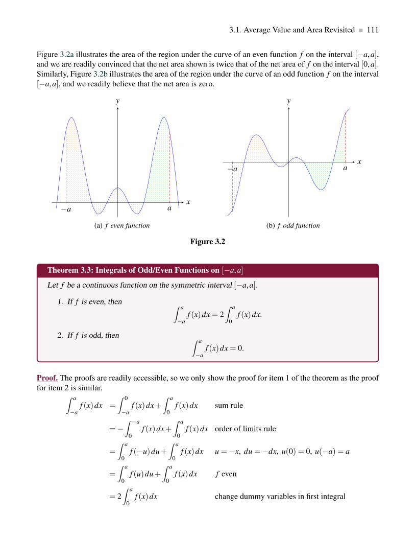
3.1. Average Value and Area Revisited 111
Figure 3.2a illustrates the area of the region under the curve of an even function f on the interval [−a,a],and we are readily convinced that the net area shown is twice that of the net area of f on the interval [0,a].Similarly, Figure 3.2b illustrates the area of the region under the curve of an odd function f on the interval
[−a,a], and we readily believe that the net area is zero.
−a ax
y
(a) f even function
−a ax
y
(b) f odd function
Figure 3.2
Theorem 3.3: Integrals of Odd/Even Functions on [−a,a]
Let f be a continuous function on the symmetric interval [−a,a].
1. If f is even, then∫ a
−af (x)dx = 2
∫ a
0f (x)dx.
2. If f is odd, then∫ a
−af (x)dx = 0.
Proof. The proofs are readily accessible, so we only show the proof for item 1 of the theorem as the proof
for item 2 is similar.∫ a
−af (x)dx =
∫ 0
−af (x)dx+
∫ a
0f (x)dx sum rule
=−∫ −a
0f (x)dx+
∫ a
0f (x)dx order of limits rule
=
∫ a
0f (−u)du+
∫ a
0f (x)dx u =−x, du =−dx, u(0) = 0, u(−a) = a
=
∫ a
0f (u)du+
∫ a
0f (x)dx f even
= 2
∫ a
0f (x)dx change dummy variables in first integral

112 Applications of Integration
♣
3.1.3. Area Between Curves: Integration w.r.t x
We have seen how integration can be used to find an area between a curve and the x-axis. With very little
change we can find some areas between curves; indeed, the area between a curve and the x-axis may be
interpreted as the area between the curve and a second “curve” with equation y = 0.
Suppose we would like to find the area below f (x) =−x2+4x+3 and above g(x) =−x3+7x2−10x+5 over the interval 1 ≤ x ≤ 2. Figure 3.3a depicts the area of the region contained between the curves of f
and g as well as the lines x = 1 and x = 2. We can see from this figure that the curve f is indeed above the
curve g on the interval [1,2].
We can approximate the area between two curves by dividing the area into thin sections and approxi-
mating the area of each section by a rectangle, as indicated in Figure 3.3b. The area of a typical rectangle
is ∆x( f (xi)−g(xi)), so the total area is approximately
n−1
∑i=0
( f (xi)−g(xi))∆x.
This is exactly the sort of sum that turns into an integral in the limit, namely the integral
∫ 2
1f (x)−g(x)dx.
Then
∫ 2
1f (x)−g(x)dx =
∫ 2
1(−x2 +4x+3)− (−x3 +7x2 −10x+5)dx
=
∫ 2
1x3 −8x2 +14x−2dx
=
[
x4
4− 8x3
3+7x2 −2x
]2
1
=
(
16
4− 64
3+28−4
)
−(
1
4− 8
3+7−2
)
= 23− 56
3− 1
4
=49
12.

3.1. Average Value and Area Revisited 113
y = f (x)
y = g(x)
1 2x
y
(a) area of region between f , g, x = 1 and x = 2
y = g(x)
1 2x
y
(b) approximating area of region with rectangles
Figure 3.3
We can also approach this problem of finding the area of the region between the curves of f and g as
well as the lines x = 1 and x = 2 by using our knowledge of the definite integrals of f and g separately.
Figure 3.4a depicts the area of the region between the curves f and the x-axis as well as the lines x = 1
and x = 2, which we know as the definite integral
∫ 2
1f (x)dx.
Similarly, Figure 3.4b depicts the area of the region between the curves g and the x-axis as well as the
lines x = 1 and x = 2, which we know as the definite integral
∫ 2
1g(x)dx.
From Figure 3.4, we can readily determine that the area of the region we want must be the area of the region
under the graph of f minus the area of the region under the graph of g as shown again in Figure 3.4c. Once
again, we have that
∫ 2
1f (x)−g(x)dx =
∫ 2
1
(
−x2 +4x+3)
−(
−x3 +7x2 −10x+5)
dx
=49
12.

114 Applications of Integration
y = f (x)
1 2x
y
(a)
∫ 2
1f (x)dx
y = g(x)
1 2x
y
(b)
∫ 2
1g(x)dx
y = f (x)
y = g(x)
1 2x
y
(c)
∫ 2
1[ f (x)−g(x)] dx
Figure 3.4
In summary, this procedure can informally be thought of as follows.
Area Between Two Curves: Integration w.r.t x
Area =
∫ b
a(top curve)− (bottom curve)dx, a ≤ x ≤ b.
y = f (x)top
y = g(x)bottom
Area
a bx
y
This leads us to the following theorem for the area of the region between two curves on a closed
interval.
Theorem 3.4: Area Between Two Curves: Integration w.r.t x
Let y = f (x) and y = g(x) be continuous functions on a closed interval [a,b] such that f (x) ≥ g(x)for all x ∈ [a,b]. Then the area A of the region between the curves of f and g as well as the lines
x = a and x = b is
A =∫ b
a[ f (x)−g(x)] dx.
Note: If we do not know which of the two functions y = f (x) and y = g(x) is larger on a given interval
[a,b], we can still ensure that we calculate the area of the region between the curves of f and g and the

3.1. Average Value and Area Revisited 115
lines x = a and x = b by placing absolute values around the integrand:
A =∫ b
a| f (x)−g(x)| dx.
Example 3.5: Area between Curves
Find the area between f (x) =−x2 +4x and g(x) = x2 −6x+5.
Solution. Here we are not given a specific interval, so it must be the case that there is a “natural” region
involved, which we see from the graph shown below. Since the curves are both parabolas, the only
reasonable interpretation is the region between the two intersection points.
We now find the intersection points by letting f (x) = g(x):
−x2 +4x = x2 −6x+5
−2x2 +10x−5 = 0
=⇒ x =5
2±
√15
2.
If we let a = (5−√
15)/2 and b = (5+√
15)/2, the total area is
∫ b
a
(
−x2 +4x)
− (x2 −6x+5)dx =
∫ b
a−2x2 +10x−5dx
= −2x3
3+5x2 −5x
∣
∣
∣
∣
b
a
= 5√
15.
after a bit of simplification.
y =−x2 +4x
y = x2 −6x+5
1 2 3 4 5
−4
−2
2
4
x
y
♣
A general guideline to compute the area between two curves follows.
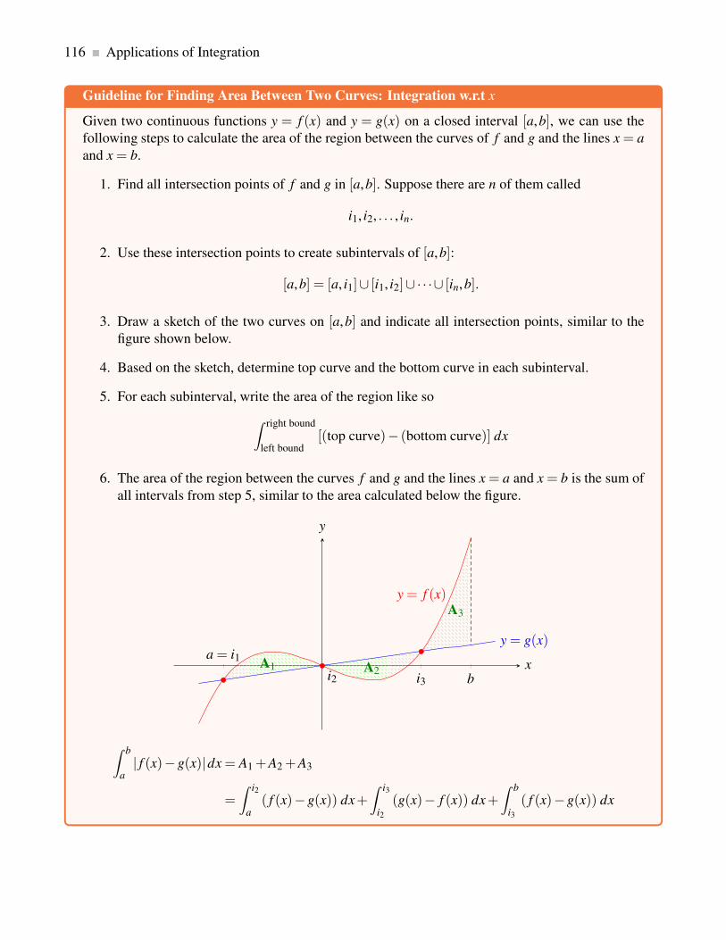
116 Applications of Integration
Guideline for Finding Area Between Two Curves: Integration w.r.t x
Given two continuous functions y = f (x) and y = g(x) on a closed interval [a,b], we can use the
following steps to calculate the area of the region between the curves of f and g and the lines x = a
and x = b.
1. Find all intersection points of f and g in [a,b]. Suppose there are n of them called
i1, i2, . . . , in.
2. Use these intersection points to create subintervals of [a,b]:
[a,b] = [a, i1]∪ [i1, i2]∪· · ·∪ [in,b].
3. Draw a sketch of the two curves on [a,b] and indicate all intersection points, similar to the
figure shown below.
4. Based on the sketch, determine top curve and the bottom curve in each subinterval.
5. For each subinterval, write the area of the region like so
∫ right bound
left bound[(top curve)− (bottom curve)] dx
6. The area of the region between the curves f and g and the lines x = a and x = b is the sum of
all intervals from step 5, similar to the area calculated below the figure.
i3 b
y = f (x)
y = g(x)a = i1
i2A1 A2
A3
x
y
∫ b
a| f (x)−g(x)|dx = A1 +A2 +A3
=∫ i2
a( f (x)−g(x)) dx+
∫ i3
i2
(g(x)− f (x)) dx+∫ b
i3
( f (x)−g(x)) dx
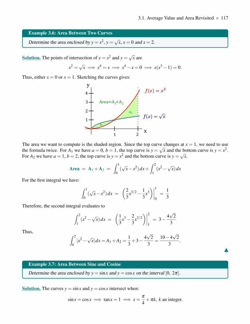
3.1. Average Value and Area Revisited 117
Example 3.6: Area Between Two Curves
Determine the area enclosed by y = x2, y =√
x, x = 0 and x = 2.
Solution. The points of intersection of y = x2 and y =√
x are
x2 =√
x =⇒ x4 = x =⇒ x4 − x = 0 =⇒ x(x3 −1) = 0.
Thus, either x = 0 or x = 1. Sketching the curves gives:
The area we want to compute is the shaded region. Since the top curve changes at x = 1, we need to use
the formula twice. For A1 we have a = 0, b = 1, the top curve is y =√
x and the bottom curve is y = x2.
For A2 we have a = 1, b = 2, the top curve is y = x2 and the bottom curve is y =√
x.
Area = A1 +A2 =∫ 1
0(√
x− x2)dx+∫ 2
1(x2 −
√x)dx
For the first integral we have:
∫ 1
0(√
x− x2)dx =
(
2
3x3/2 − 1
3x3
)∣
∣
∣
∣
1
0
=1
3
Therefore, the second integral evaluates to
∫ 2
1(x2 −
√x)dx =
(
1
3x3 − 2
3x3/2
)∣
∣
∣
∣
2
1
= 3− 4√
2
3
Thus,∫ 2
0|x2 −
√x|dx = A1 +A2 =
1
3+3− 4
√2
3=
10−4√
2
3.
♣
Example 3.7: Area Between Sine and Cosine
Determine the area enclosed by y = sinx and y = cosx on the interval [0, 2π ].
Solution. The curves y = sinx and y = cosx intersect when:
sinx = cosx =⇒ tanx = 1 =⇒ x =π
4+πk, k an integer.

118 Applications of Integration
We have the following sketch:
The area we want to compute is the shaded region. The top curve changes at x = π/4 and x = 5π/4, thus,
we need to split the area up into three regions: from 0 to π/4; from π/4 to 5π/4; and from 5π/4 to 2π .
Area =
∫ π4
0(cosx− sinx)dx+
∫ 5π4
π4
(sinx− cosx)dx+
∫ 2π
5π4
(cosx− sinx)dx
= (sinx+ cosx)
∣
∣
∣
∣
π/4
0
+(−cosx− sinx)
∣
∣
∣
∣
5π/4
π/4
+(sinx+ cosx)
∣
∣
∣
∣
2π
5π/4
=(√
2−1)
+(√
2+√
2)
+(
1+√
2)
= 4√
2
♣
3.1.4. Area Between Curves: Integration w.r.t. y
Sometimes the given curves are not functions of x. Instead, the area of the region is between two functions
of y, namely x = f (y) and x = g(y), and the lines y = c and y = d, which can be thought of informally as
the following.
Area Between Two Curves: Integration w.r.t. y
Area =∫ d
c(right curve)− (left curve)dy, c ≤ y ≤ d.
x = f (y)right
x = g(y)left
Area
c
d
x
y
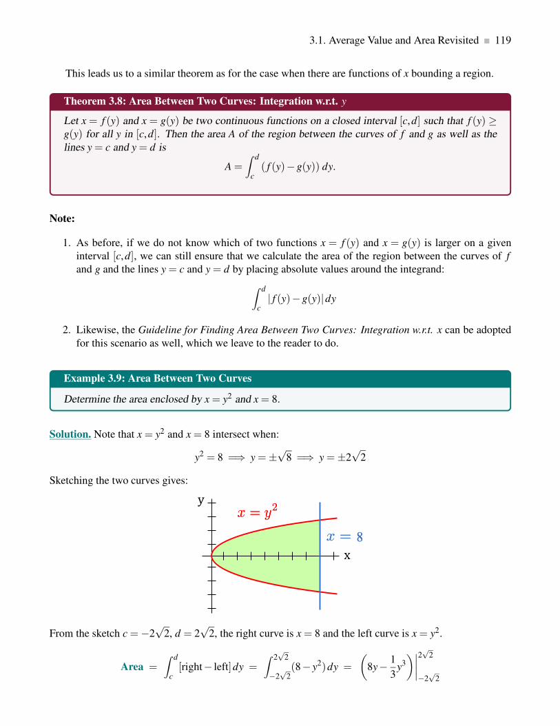
3.1. Average Value and Area Revisited 119
This leads us to a similar theorem as for the case when there are functions of x bounding a region.
Theorem 3.8: Area Between Two Curves: Integration w.r.t. y
Let x = f (y) and x = g(y) be two continuous functions on a closed interval [c,d] such that f (y) ≥g(y) for all y in [c,d]. Then the area A of the region between the curves of f and g as well as the
lines y = c and y = d is
A =∫ d
c( f (y)−g(y)) dy.
Note:
1. As before, if we do not know which of two functions x = f (y) and x = g(y) is larger on a given
interval [c,d], we can still ensure that we calculate the area of the region between the curves of f
and g and the lines y = c and y = d by placing absolute values around the integrand:
∫ d
c| f (y)−g(y)|dy
2. Likewise, the Guideline for Finding Area Between Two Curves: Integration w.r.t. x can be adopted
for this scenario as well, which we leave to the reader to do.
Example 3.9: Area Between Two Curves
Determine the area enclosed by x = y2 and x = 8.
Solution. Note that x = y2 and x = 8 intersect when:
y2 = 8 =⇒ y =±√
8 =⇒ y =±2√
2
Sketching the two curves gives:
From the sketch c =−2√
2, d = 2√
2, the right curve is x = 8 and the left curve is x = y2.
Area =∫ d
c[right− left]dy =
∫ 2√
2
−2√
2(8− y2)dy =
(
8y− 1
3y3
)∣
∣
∣
∣
2√
2
−2√
2

120 Applications of Integration
=
[
8(2√
2)− 1
3(2√
2)3
]
−[
8(−2√
2)− 1
3(−2
√2)3
]
=64
√2
3
We could have also integrated w.r.t. x by using the two functions y =√
x and y =−√x. We leave it to
the reader to follow up on this integration. ♣
Exercises for Section 3.1
Exercise 3.1.1 Find the average height of f (x) over the given interval(s).
(a) f (x) = cosx on [0,π/2], [−π/2,π/2], and [0,2π ]
(b) f (x) = x2 on [−2,2]
(c) f (x) =1
x2on [1,a]
(d) f (x) =√
1− x2 on [−1,1]
Exercise 3.1.2 Find the area bounded by the curves by integrating with respect to x.
(a) y = x4 − x2 and y = x2 (the part to the right of the y-axis)
(b) y = cos(πx/2) and y = 1− x2 (in the first quadrant)
(c) y = sin(πx/3) and y = x (in the first quadrant)
(d) y =√
x and y = x2
(e) y = x3/2 and y = x2/3
(f) y = x2 −2x and y = x−2
Exercise 3.1.3 Find the area bounded by the curves by integrating with respect to y.
(a) x = y3 and x = y2
(b) x = 0 and x = 25− y2
Exercise 3.1.4 Find the area bounded by the curves.
(a) x = 1− y2 and y =−x−1
(b) x = 3y− y2 and x+ y = 3
(c) y =√
x and y =√
x+1, 0 ≤ x ≤ 4

3.1. Average Value and Area Revisited 121
(d) y = sinxcosx and y = sinx, 0 ≤ x ≤ π
Exercise 3.1.5 Find the area bounded by the given curves.
3
y = x3 −3x2
y = 0
(a)
x
y
3
y = x4 −3x3
y = 0
(b)
x
y
−2 2
−2
2
y = x√
4− x2
y = 0
(c)
x
y
−1 1
y =3x
x2 +1
y = 0
(d)
x
y
9
y =x
3−√
x
y = 0
(e)
x
y
y =−1
2+ x
y =√
x/4
( f )
1x
y
Exercise 3.1.6 An object moves so that its velocity at time t is v(t) =−9.8t+20 m/s. Describe the motion
of the object between t = 0 and t = 5, find the total distance travelled by the object during that time, and
find the net distance travelled.
Exercise 3.1.7 An object moves so that its velocity at time t is v(t) = sint. Set up and evaluate a single
definite integral to compute the net distance travelled between t = 0 and t = 2π .

122 Applications of Integration
Exercise 3.1.8 An object moves so that its velocity at time t is v(t) = 1+2sint m/s. Find the net distance
travelled by the object between t = 0 and t = 2π , and find the total distance travelled during the same
period.
Exercise 3.1.9 Consider the function f (x) = (x+2)(x+1)(x−1)(x−2) on [−2,2]. Find the total area
between the curve and the x-axis (measuring all area as positive).
Exercise 3.1.10 Consider the function f (x) = x2 −3x+2 on [0,4]. Find the total area between the curve
and the x-axis (measuring all area as positive).
Exercise 3.1.11 Evaluate the three integrals:
A =
∫ 3
0(−x2 +9)dx B =
∫ 4
0(−x2 +9)dx C =
∫ 3
4(−x2 +9)dx,
and verify that A = B+C. Draw a diagram which illustrates this relationship.
3.2 Applications to Business and Economics
Just like the process of differentiation is a useful tool in many business and economics applications such
as problems related to elasticity of demand and optimization, so is the process of antidifferentiation or in-
tegration. In this section, we revisit two important business and economic models, namely concerning law
of supply and demand in a free-market environment and continuous money flow, and introduce integration
as a method for solving problems of this nature.
3.2.1. Surplus in Consumption and Production
Recall that in a free market, the consumer demand for a particular commodity is dependent on the com-
modity’s unit price, which is captured graphically by the demand curve. As expected, the quantity de-
manded of a commodity increases as the commodity’s unit price decreases, and vice versa. Similarly, the
unit price of a commodity is dependent on the commodity’s availability in the market, which is articulated
graphically by the supply curve. Typically, an increase or decrease in the commodity’s unit price induces
the producer to respectively increase or decrease the supply of the commodity. Below we see the supply
and demand curves of a certain item produced and sold:

3.2. Applications to Business and Economics 123
xe
pe (xe, pe)
x
p
Figure 3.5: Example of a supply curve (in blue) and a demand curve (in red). The point of intersec-
tion (xe, pe) corresponds to market equilibrium.
In a competitive market, the price of a commodity will eventually settle at the market equilibrium,
which occurs when the supply of the commodity will be equal to its demand as indicated with the point
(xe, pe) in Figure 3.5. Let us look at a certain commodity, say, dairy to discuss the economic significance of
the market equilibrium. As long as p < pe, then the demand for dairy exceeds its supply (see Figure 3.5),
which pushes up the price until it reaches the equilibrium price pe, which in turn signifies that the quantity
supplied is equal to the quantity demanded, namely xe. On the other hand, if p > pe, then the supply
of dairy exceeds demand (see Figure 3.5), which brings the price down. In an ideal free market, buying
and selling at the equilibrium price should benefit both consumers and producers. In this section, we will
compute the surplus, which tells us exactly how much the consumers save and the producers gain by
buying and selling respectively at the equilibrium price rather than at a higher price.
We begin by computing exactly how much consumers spent when they buy at the equilibrium price
pe:
total amount spent at equilibrium price
= (number of units bought at equilibrium price) · (unit price)
= xe · pe
The quantity xe · pe is the rectangular area shown in Figure 3.6a.
Now we compute the total amount that would be spent if every consumer paid the maximum price that
each is willing to pay. Given a demand function D, partition the interval [0,xe] into n subintervals of equal
width ∆x = xen with endpoints xi =
ixen , i = 0,1, . . . ,n as shown below:

124 Applications of Integration
demand D
(xe, pe)
. . .
x1 x2 xe
pn = pe
p2p1
x
p
Now, let us analyze this partition subinterval by subinterval. Suppose that only x1 units had been
available, then the maximum unit price could have been set at D(x1) dollars and a total of x1 units would
be sold, but at this price no further units would have been sold. Then the total expenditure in dollars is
given by
(price per unit) · (number of units) = D(x1) ·∆x.
Now suppose that more units become available by producing x2 units of our commodity. If the maximum
price is set at D(x2) dollars, then the remaining x2−x1 = ∆x units can be sold at a cost of D(x2) ·∆x dollars.
If we continue with this process of price discrimination, then the total amount spent at maximum price is
approximately equal to
D(x1) ·∆x+D(x2) ·∆x+ · · ·+D(xn) ·∆x.
Note:
1. On each of the subintervals [0,x1], [x1,x2], . . . , [xn−1,xe], the buyers paid as much for each unit as it
was worth to them.
2. We recognize that the last sum is a Riemann sum, which yields
∫ xe
0D(x)dx as n→∞ or alternatively
as ∆x → 0.
Of course, we simply have calculated the area under the demand curve on the interval [0,xe], which is
shown in Figure 3.6b.
xe
pe
SupplyDemand
equilibrium
x
p
(a)
xe
pe
SupplyDemand
equilibrium
x
p
(b)
xe
pe
SupplyDemand
equilibriumconsumer
surplus
x
p
(c)
Figure 3.6: Consumer expenditure on [0,xe] at equilibrium price, in total, and for surplus.

3.2. Applications to Business and Economics 125
The difference between the total amount spent at the maximum price (Figure 3.6b) and the consumer
expenditure at the equilibrium price (Figure 3.6a) is the total amount that consumers save by buying at
the equilibrium price (Figure 3.6c). This saving is called the consumer surplus for this product. We
summarize our result.
Theorem 3.10: Consumer Surplus
Let D be the demand function, pe be the equilibrium price, and xe be the equilibrium quantity sold.
Then the consumer surplus is
∫ xe
0D(x)dx− xe pe =
∫ xe
0[D(x)− pe] dx.
In a similar manner, we can determine how much producers gain when they sell at the equilibrium
price pe:
total amount gained at equilibrium price
= (number of units sold at equilibrium price) · (unit price)
= xe · pe
Now we compute the total amount that would be gained if every producer sold at the minimum amount
they are willing to accept for the product. Given a supply function S, partition the interval [0,xe] into n
subintervals of equal width ∆x = xen with endpoints xi =
ixen , i = 0,1, . . . ,n as shown below:
supply S
(xe, pe)
. . .
x1 x2 xe
p1p2
pn = pe
x
p
Similarly to the subinterval by subinterval analysis for the demand curve, an analysis of the partition
of the supply curve shows that the total revenue on every subinterval in dollars by selling at the minimum
price is given by
(price per unit) · (number of units) = S(xi) ·∆x
for i= 1,2, . . . ,n. Continuing with the process of price discrimination, the total amount gained at minimum
price is approximately equal to
S(x1) ·∆x+S(x2) ·∆x+ · · ·+S(xn) ·∆x.
Note:

126 Applications of Integration
1. On each of the subintervals [0,x1], [x1,x2], . . . [xn−1,xe], the producers sold at the lowest price that
they are willing to set.
2. This sum is again a Riemann sum, which yields
∫ xe
0S(x)dx as n → ∞ or alternatively as ∆x → 0.
Figure 3.7b shows the area under the supply curve on the interval [0,xe] that our computation has yielded.
xe
pe
SupplyDemand
equilibrium
x
p
(a)
xe
pe
SupplyDemand
equilibrium
x
p
(b)
xe
pe
SupplyDemand
equilibrium
producer
surplus
x
p
(c)
Figure 3.7: Producer revenue on [0,xe] at equilibrium price, in total, and for surplus.
The difference between the producer revenue at the equilibrium price (Figure 3.7a) and the total
amount achieved at the minimum price (Figure 3.7b) is the total amount that producers gain by selling
at the equilibrium price (Figure 3.7c). This income is called the producer surplus for this product. We
summarize our result.
Theorem 3.11: Producer Surplus
Let S be the supply function, pe be the equilibrium price, and xe be the equilibrium quantity sold.
Then the producer surplus is
xe pe −∫ xe
0S(x)dx =
∫ xe
0[pe −S(x)] dx.
Note: In general, the consumer surplus and the producer surplus are not equal.
Example 3.12: Consumer Surplus
The demand for a product, in dollars, is
p = D(x) = 1000−0.5x−0.0002x2.
Find the consumer surplus when the sales level is 200.
Solution. When the number of units sold is xe = 200, the corresponding price is
pe = 1000−0.5(200)−0.0002(2002) = 892.

3.2. Applications to Business and Economics 127
Therefore, the consumer surplus is
∫ 200
0[D(x)− pe] dx =
∫ 200
0
(
1000−0.5x−0.0002x2 −892)
dx
=∫ 200
0
(
108−0.5x−0.0002x2)
dx
=
[
108x−0.25x2 − 0.0002
3x3
]200
0
= 108(200)−0.25(200)2− 0.0002
3(200)3
= $11,066.70
♣
Example 3.13: Consumer and Producer Surplus
The price, in dollars per kg, of flour at a certain grocer is given by
D(x) = 75− e0.2x, for x ∈ [0,21]
corresponding to a demand of x kg. When the supply is x kg, the wholesale price is given by
S(x) = 2e0.2x −1.
Determine the consumer surplus and the producer surplus.
Solution. We set D(x) = S(x) to find the equilibrium quantity and price:
75− e0.2x = 2e0.2x −1
e0.2x =76
3
x =ln(
763
)
0.2≈ 16.16 kg.
Therefore, the equilibrium point is
(xe, pe) = (16.16,75− e0.2(16.16))≈ (16.16,49.67).
We now calculate the consumer surplus as
∫ 16.16
0
[
(75− e0.2x)−49.67]
dx =∫ 16.16
0
(
25.33− e0.2x)
dx
=
[
25.33x− 1
0.2e0.2x
]16.16
0
≈ $287.68.

128 Applications of Integration
Similarly, we calculate the producer surplus as
∫ 16.16
0
[
49.67−(
2e0.2x −1)]
dx =
∫ 16.16
0
(
50.67−2e0.2x)
dx
=
[
50.67x− 2
0.2e0.2x
]16.16
0
≈ $575.53.
Thus, the consumer surplus is approximately $287.68 and the producer surplus is approximately $575.53.
These quantities are illustrated in the figure below.
5 10 15 20
20
40
60
80
100
D(x)
S(x)
(16.16,49.67)
consumer
surplus
producer
surplus
x (kg)
p ($)
♣
3.2.2. Continuous Money Flow
Another application of integrals is for the computation involved in continuous money flow problems.
These problems may be payments to repay a debt or deposits to establish a retirement plan that are made
at regular monthly payments over a certain time period. If the time between deposits or payments are made
in relatively short intervals compared to the entire time period, then the money can be thought of as flowing
continuously, hence the name continuous money flow. Some textbooks refer to these types of problems as
“continuous income streams” or “continuous money streams”. Naturally, deposits or payments cannot be
made continuously in a physical manner, since the units of legal tender are by their very nature discrete
such as the cent and dollar.
A word of caution: Discussing the value of money is difficult as there are many parameters affecting
it. For the purpose of this introductory section, we take a simplified point of view such as assuming that
there is a single interest rate, no inflation, and no other factors influencing computation. This simplified
approach will provide for an intuitive understanding of solving continuous money flow problems that can
then be expanded upon. Before we develop formulas for the present and future value of such a continuous
money flow, we begin by computing the total amount of money that is being accumulated making the
regular deposits or payments.

3.2. Applications to Business and Economics 129
T
m
t
f (t)
(a) A uniform rate of money flow f (t) =m dollars per year.
Tt
f (t)
(b) A variable rate of money flow f (t) dollars per year.
Figure 3.8
Suppose that f (t) is the rate in dollars per unit of time for a continuous money flow. Figure 3.8 above
shows a uniform rate of money flow f (t) = m dollars per year to the left and a variable rate of money flow
f (t) dollars per year to the right. The total income in dollars of the former case can be readily calculated
and is simply the rectangular area m ·T dollars. For the latter case, we readily understand that the area
under the curve f from t = 0 to t = T is the total income, whose value in dollars is determined by the
definite integral
∫ T
0f (t)dt.
Theorem 3.14: Total Income of Money Flow
Suppose that f (t) is the rate in dollars per unit of time for a continuous money flow. Then the total
income I over the time period [0,T ] is
I =∫ T
0f (t)dt.
Note: The above computation does not calculate the accumulated interest, just the total income.
Example 3.15: Total Income
Suppose the income of a small coffee shop projected to grow exponentially. The rate of income
when the shop first opened was at $5,000 per month, which grew to a rate of $6,000 per month by
the second month. What is the expected total income from the coffee shop during its first 6 months
of operation?
Solution. Let t be the time in months since the opening of the shop. The projected income is of the form
f (t) =Cekt .

130 Applications of Integration
Since f (0) = 5000, we must have C = 5000. Now to determine k, we use f (1) = 6000:
5000ek(1) = 6000
k = ln6000
5000
k ≈ 0.18.
Thus, f (t) = 5000e0.18t . We can now determine the total income, I:
I =
∫ 6
0f (t)dt
=
∫ 6
05000e0.18t dt
=5000
0.18e0.18t
∣
∣
6
0
≈ 54018.8764.
We conclude that the coffee shop is expected to produce an income of approximately $54,018.88 in its
first six months of operation. ♣
Let us now develop the formulas for the present value and future value of a continuous money flow. We
begin by summarizing the present and future value of money that earns interest compounded continuously
at a rate r over time t without making continuous deposits or payments. Suppose that F is the amount of
money at time t that accumulates interest compounded continuously at a rate r over time t, then the interest
earned over time is described by the differential equation
dF
dt= rF .
In Chapter 5, differential equations will be discussed in more detail, but for now, we simply present
the solution to this differential equation, and so the future value is described by
F(t) = Pert ,
where P is the initial amount. Similarly, if we want to obtain an amount of F dollars that has accrued
interest compounded continuously at the annual rate r over t years, then the amount of money that needs
to be deposited today, namely the present value P, is given by
P(t) = Fe−rt .
Now, the present value P of a continuous money stream must be the amount of money that will
accumulate to the same future value as the continuous money when deposited at the same interest rate
compounded continuously for the same period of time but without the continuous stream of income. Let
f (t) represent the rate of continuous money flow and r the rate of interest for T years. As usual, we
partition the interval [0,T ] into n subintervals of equal width ∆t = Tn with endpoints ti =
iTn , i = 0,1, . . . ,n
as shown below.

3.2. Applications to Business and Economics 131
∆t
ti tn = T
f (ti)
t
f (t)
Using our result from above about accruing interest compounded continuously, the present value Pi of
the money flow over the i-th subinterval is approximately
Pi = [ f (ti)∆t]e−rti ,
and so the total present value is approximated by a typical Riemann sum
P =n
∑i=1
[ f (ti)∆t]e−rti .
Taking the limit as n → ∞, we obtain the following definite integral
P =
∫ T
0f (t)e−rt dt.
We capture our result in the following theorem.
Theorem 3.16: Present Value of a Continuous Money Flow
Suppose that f (t) is the rate of money flow in dollars per unit of time that is earning interest com-
pounded continuously at a rate r per unit of time over the time period [0,T ]. Then the present value
P of this continuous money flow is
P =
∫ T
0f (t)e−rt dt.
Before we develop the formula for the accumulated amount of a continuous money flow, we present
one example of a present value problem.
Example 3.17: Present Value
A certain manufacturer produces industrial bread-making machines, which are estimated to generate
a continuous income stream each with a rate of 28 − 4.5t million dollars per year in year t of
operation. Each machine is in operation for about 6 years and the money is invested at the annual
rate of 5% compounded continuously. Compute the fair market price of each machine.

132 Applications of Integration
Solution. We assume that the fair market price of each machine is the present value of the continuous
money flow with
f (t) = 28−4.5t, r = 0.05, and T = 6.
Therefore, the price P is given by
P =∫ 6
0[28−4.5t]e−0.05t dt =
∫ 6
028e−0.05t dt −4.5
∫ 6
0te−0.05t dt.
The first integral can be computed directly
∫ 6
028e−0.05t dt =
[
− 28
0.05e−0.05t
]6
0
= 560(
1− e−0.03)
.
The second integral can be solved using Integration by Parts, with
u = t, dv = e−0.05tdt =⇒ du = dt, v =− 1
0.05e−0.05t
to obtain
∫ 6
0te−0.05t dt =
[
− t
0.05e−0.05t
]6
0+
1
0.05
∫ 6
0e−0.05t dt
=−[
0.05t +1
0.05e−0.05t
]6
0
= 20−26e−0.3.
Hence,
P =∫ 6
0[28−4.5t]e−0.05t dt
= 560(
1− e−0.3)
−4.5(
20−26e−0.3)
≈ 141.82,
and so the fair market price of each machine is about 142 million dollars. ♣
Similarly, we can develop a formula for the future value of a continuous money flow. Again, we
partition the interval [0,T ] into n subintervals of equal width ∆t = Tn with endpoints ti =
iTn , i = 0,1, . . . ,n.
Now, the money that is deposited or paid during the i-th time interval stays in the account for the length of
time T − ti. Using our result from the beginning of this section about interest being earned compounded
continuously, the future value Fi of the money flow over the i-th subinterval is approximately
Fi = [ f (ti)∆t]er(T−ti),
and so the total future value is again approximated by a Riemann sum, namely
F =n
∑i=1
[ f (ti)∆t]er(T−ti).
Taking the limit as n → ∞, the following definite integral is obtained
F =∫ T
0f (t)er(T−t) dt.

3.2. Applications to Business and Economics 133
This leads to the following theorem.
Theorem 3.18: Future Value of a Continuous Money Flow
Suppose that f (t) is the rate of money flow in dollars per unit of time that is earning interest com-
pounded continuously at a rate r per unit of time over the time period [0,T ]. Then the future value
F of this continuous money flow is
F =
∫ T
0f (t)er(T−t) dt.
Example 3.19: Continuous Money Flow
Suppose money is flowing continuously at a constant rate f (t) for 10 years at 8% interest com-
pounded continuously accumulating to $20,000. Compute f (t).
Solution. We have that
F = 20,000, r = 0.08, and T = 10.
We can use the formula for the future value to solve for the rate f (t) of the continuous money flow:
20,000 =∫ 10
0f (t)e0.08(10−t) dt
Since the rate of money flow is constant, f (t) does not depend on t. Therefore, f (t) can be taken out of
the integral as follows.
20,000 = f (t)
∫ 10
0e0.08(10−t) dt
−0.08 · e−0.8 ·20,000 = f (t)[
e−0.08t]10
0
−0.08 · e−0.8 ·20,000 = f (t)[
e−0.8 − e0]
f (t) =0.08 ·20,000
[e0.8 −1]≈ $1305.55
♣
Example 3.20: Total Income, Present and Future Values
Suppose money is flowing continuously at a constant rate of $3500 per year for 10 years at 1.25%
interest compounded continuously. Compute the following:
(a) total income;
(b) future value at T = 10 years;
(c) total interest; and
(d) present value.
Solution. We have that f (t) = 3500, r = 0.0125, and T = 10.

134 Applications of Integration
(a) The total income I is given by
I =∫ 10
03500dt = $35,000.
(b) The future value F at T = 10 years is calculated to be
F =∫ 10
03500e0.0125(10−t) dt =− 3500
0.0125
[
e0.0125(10−t)]10
0= $37,281.75
(c) The total interest is the difference between the future value F at T = 10 years and the total income
over 10 years:
$37,281.75−$35,000 = $2281.57.
(d) The present value P is obtained as
P =∫ 10
03500e−0.0125t dt
=
[
− 3500
0.0125e−0.0125
]10
0
=3500
0.0125
(
1− e−0.125)
≈ $39,900.87.
♣
Exercises for Section 3.2
Exercise 3.2.1 Suppose the supply function for a certain product is given by
S(q) = q5/2 +3q1/2 +25.
If the equilibrium quantity is q = 10, determine the producer surplus.
Exercise 3.2.2 It is determined that the supply function for a certain nutritional supplement can be de-
scribed by
S(x) = x3/2 +2x1/2 +50.
Assuming that the supply and demand are in equilibrium when x = 12, determine the producer surplus.
Exercise 3.2.3 Determine the consumer surplus corresponding to the demand function
D(q) =100
(q+2)2,
if the equilibrium quantity is q = 2.

3.2. Applications to Business and Economics 135
Exercise 3.2.4 Suppose the demand function for organic tomatoes can be described by
D(x) =20,000
(2x+5)3.
Determine the consumer surplus if the supply and demand are in equilibrium at x = 4.
Exercise 3.2.5 The supply function for steel-cut oats is found to be
S(q) = q(2q+25),
dollars and the demand function is found to be
D(q) = 1000−10q−q2,
dollars, where q is measured in kgs.
(a) Determine the equilibrium point.
(b) What is the consumer surplus?
(c) What is the producer surplus?
(d) Display your results on a graph of the supply and demand curves.
Exercise 3.2.6 It is determined that the supply function for a certain product x (measured in units of
thousands) can be described by
S(x) =
(
2x+1
4
)2
,
with a corresponding demand function
D(x) =200
15x+1.
(a) Determine the equilibrium point.
(b) What is the consumer surplus?
(c) What is the producer surplus?
(d) Display your results on a graph of the supply and demand curves.
Exercise 3.2.7 For each of the following rate of money flow in dollars per year, rate r of continuously
compounded interest, and time period T years, compute (i) the total income; (ii) the future value at T ; (iii)
the total interest; and (iv) the present value.
(a) f (t) = 200, r = 2%, T = 5.
(b) f (t) = 4000, r = 0.5%, T = 7.
(c) f (t) = 10,000, r = 1%,T = 4.
(d) f (t) = 300t, r = 1%,T = 4.
136 Applications of Integration
(e) f (t) = 450e0.5t , r = 1.5%,T = 15. (f) f (t) = 100t +50, r = 3%, T = 9.
Exercise 3.2.8 The value of a continuous money flow is found to be $5,000 after 6 years. Assume the rate
of money flow f (t) is constant, and the interest is continuously compounded at a rate of 1%. Compute
f (t).
Exercise 3.2.9 The value of a continuous money flow is found to be $10,000 after 5 years, and $14,000
after 7 years. The rate of money flow f (t) is linear, and the interest is compounded continuously at a rate
of 1.5%. Compute f (t).
3.3 Volume of Revolution: Disk Method
We have seen how to compute certain areas by using integration; we will now look into how some volumes
may also be computed by evaluating an integral. Generally, the volumes that we can compute this way
have cross-sections that are easy to describe. For example, circular cross-sections are easy to describe as
their area just depends on the radius, and so they are one of the central topics in this section. However, we
first discuss the general idea of calculating the volume of a solid by slicing up the solid.
3.3.1. Computing Volumes with Cross-sections
Let us first formalize what is meant by a cross-section.
Definition 3.21: Cross-section
A cross-section of a solid is the region obtained by intersecting the solid with a plane.
Examples of cross-sections are the circular region above the right cylinder in Figure 3.9a, the star above
the star-prism in Figure 3.9b, and the square we see in the pyramid on the left side of Figure 3.10. For
now, we are only interested in solids, whose volumes are generated through cross-sections that are easy to
describe. For example, the right cylinder in Figure 3.9a is generated by translating a circular region along
the x-axis for a certain length h. Every cross-section of the right cylinder must therefore be circular, when
cutting the right cylinder anywhere along length h that is perpendicular to the x-axis.

3.3. Volume of Revolution: Disk Method 137
(a) Translated disk. (b) Translated star.
Figure 3.9
In a similar manner, many other solids can be generated and understood as shown with the translated
star in Figure 3.9b.
The volume of both the right cylinder and the translated star can be thought of as
V = (area of cross-section) · (length) = A ·h.
Let us now turn towards the calculation of such volumes by working through two examples. The right
pyramid with square base shown in Figure 3.10 has cross-sections that must be squares if we cut the
pyramid parallel to its base. The following example makes use of these cross-sections to calculate the
volume of the pyramid for a certain height.
...
Figure 3.10: Volume of a pyramid approximated by rectangular prisms.
Example 3.22: Volume of a Pyramid
Find the volume of a pyramid with a square base that is 20 meters tall and 20 meters on a side at the
base.
Solution. As with most of our applications of integration, we begin by asking how we might approximate
the volume. Since we can easily compute the volume of a rectangular prism (that is, a “box”), we will
use some boxes to approximate the volume of the pyramid, as shown in Figure 3.10: Suppose we cut up
the pyramid into n slices. On the left is a 3D view that shows cross-sections cut parallel to the base of the
pyramid and replaced with rectangular boxes that are used to approximate the volume. On the right is a

138 Applications of Integration
2D view that now shows a cross-section perpendicular to the base of the pyramid so that we can identify
the width and height of a box.
Having to use width and height means that we have two variables. However, by overlaying a Cartesian
coordinate system with the origin at the midpoint of the base on to the 2D view of Figure 3.10 as shown
below, we can relate these two variables to each other.
∆y(xi,yi)
-10 10
20
x
y
Since the cross-sectional view is placed symmetrically about the y-axis, we see that a height of 20 is
achieved at the midpoint of the base. Thus at x = 0, y = 20, at x = 10, y = 0, and we have a slope of
m =−2. So
y =−2x+b
20 =−2(0)+b
20 = b.
Therefore, y = 20− 2x, and in the terms of x we have that x = 10− y/2. We could have also used
similar triangles here to derive the relationship between x and y. From the right diagram in Figure 3.10,
we see that each box has volume of the form
(2xi)(2xi)∆y.
Then the total volume is approximately
n−1
∑i=0
(2xi)(2xi)∆y =n−1
∑i=0
4(10− yi
2)2∆y
and when we apply the limit ∆y → 0 we get the volume as the value of a definite integral as defined in

3.3. Volume of Revolution: Disk Method 139
Section 1.4:
V = lim∆y→0
n−1
∑i=0
4(10− yi
2)2∆y =
∫ 20
04(10− y
2)2 dy
=
∫ 20
0(20− y)2 dy
= −(20− y)3
3
∣
∣
∣
∣
20
0
=−03
3−(
−203
3
)
=8000
3.
As you may know, the volume of a pyramid is given by the formula
(1/3)(height)(area of base).
Using this formula we calculate
(1/3)(20)(400) =8000
3,
which agrees with our answer. ♣
Example 3.23: Volume of an Object
The base of a solid is the region between f (x) = x2 −1 and g(x) =−x2 +1 as shown to the right of
Figure 3.11, and its cross-sections perpendicular to the x-axis are equilateral triangles, as indicated
in Figure 3.11 to the left.
The solid has been truncated to show a triangular cross-section above x = 1/2.
Find the volume of the solid.
y = f (x)
y = g(x)
x = 12
-1 1
-1
1
x
y
Figure 3.11: Solid with equilateral triangles as cross-sections.
Solution. We begin by drawing the equilateral triangle above any xi and identify its base and height as
shown below to the left.

140 Applications of Integration
√3g(xi)
xif (xi) g(xi) ∆x
(xi,g(xi))
(xi, f (xi))
-1 1
-1
1
x
y
The equilateral triangle has base
g(xi)− f (xi) = (1− x2i )− (x2
i −1) = 2(1− x2i ),
and height √3g(xi) =
√3(1− x2
i ).
So the area of the cross-section is
1
2(base)(height) = (1− x2
i )√
3(1− x2i ).
The diagram above to the right indicates the position of an arbitrary thin equilateral triangle in the given
region. Therefore, the volume of this thin equilateral triangle is given by
1
2(base)(height)(thickness) = (1− x2
i )√
3(1− x2i )∆x.
If we have sliced our solid into n thin equilateral triangles, then the volume can be approximated with the
sumn−1
∑i=0
(1− x2i )√
3(1− x2i )∆x =
n−1
∑i=0
√3(1− x2
i )2∆x.
Similar to the previous example, when we apply the limit ∆x → 0, the total volume is
V = lim∆x→0
n−1
∑i=0
√3(1− x2
i )2∆x =
∫ 1
−1
√3(1− x2)2 dx =
16
15
√3.
Notice that the limits of integration, namely -1 and 1, are the left and right bounding values of x, because
we are slicing the solid perpendicular to the x-axis from left to right. ♣
3.3.2. Disk Method: Integration w.r.t. x
One easy way to get “nice” cross-sections is by rotating a plane figure around a line, also called the axis of
rotation, and therefore such a solid is also referred to as a solid of revolution. For example, in Figure 3.12

3.3. Volume of Revolution: Disk Method 141
we see a plane region under a curve and between two vertical lines x = a and x = b, which creates a solid
when the region is rotated about the x-axis, and naturally, a typical cross-section perpendicular to the x-axis
must be circular as shown.
a bx
y
Figure 3.12: A solid of rotation.
Of course a real “slice” of this figure will not be cylindrical in nature, but we can approximate the
volume of the slice by a cylinder or so-called disk with circular top and bottom and straight sides parallel
to the axis of rotation; the volume of this disk will have the form πr2∆x, where r is the radius of the disk
and ∆x is the thickness of the disk. As long as we can write r in terms of x we can compute the volume by
an integral. Often, the radius r is given by the height of the function, i.e. r = f (xi) and so we compute the
volume in a similar manner as in Section 3.3.1:
Suppose there are n disks on the interval [a,b], then the volume of the solid of revolution is approxi-
mated byn−1
∑i=0
π [ f (xi)]2 ∆x,
and when we apply the limit ∆x → 0, the volume computes to the value of a definite integral
V = lim∆x→0
n−1
∑i=0
π [ f (xi)]2 ∆x =
∫ b
aπ [ f (x)]2 dx.
Because the volume of the solid of revolution is calculated using disks, this type of computation is often
referred to as the Disk Method.
We capture our results in the following theorem.

142 Applications of Integration
Theorem 3.24: Disk Method: Integration w.r.t. x
Suppose f is non-negative and continuous on the interval [a,b]. Then the volume V formed by
rotating the area under the curve of f about the x-axis is
V = lim∆x→0
n−1
∑i=0
π [ f (xi)]2 ∆x =
∫ b
aπ [ f (x)]2 dx.
where
xi is the location of the disk,
f (xi) is the radius of the disk, and
∆x is the thickness of the disk as shown below.
∆x
y = f (x)
(xi, f (xi))
a xi b
f (xi)
x
y
f (xi)
∆x
Note: Either of the variations 1 and 2 described below will most likely create disks with holes in the solid
of revolution, and so we would have to apply the so-called Washer Method that is described in the next
section.
1. We could rotate the area of any region around an axis of rotation, including the area of a region
bounded above by a function y = f (x) and below by a function y = g(x) on an interval x ∈ [a,b].
2. The axis of rotation can be any axis parallel to the x-axis for this method to work.
We now provide one further example of the Disk Method.
Example 3.25: Volume of a Right Circular Cone
Find the volume of a right circular cone with
(a) base radius 10 and height 20.
(b) base radius r and height h.
(A right circular cone is one with a circular base and with the tip of the cone directly over the centre
of the base.)

3.3. Volume of Revolution: Disk Method 143
Solution.
(a) We can view this cone as produced by the rotation of the line y = x/2 rotated about the x-axis, as
indicated below.
∆x
xi 20
f (xi)
10
x
y
At a particular point on the x-axis, say xi, the radius of the resulting cone is the y-coordinate of the
corresponding point on the line, namely yi = xi/2. Thus the total volume is approximately
n−1
∑i=0
π(xi/2)2 dx
and the exact volume is∫ 20
0π
x2
4dx =
π
4
x3
3
∣
∣
∣
∣
20
0
=π
4
203
3=
2000π
3.
(b) Note that we can instead do the calculation with a generic height and radius:
∫ h
0π
r2
h2x2 dx =
πr2
h2
h3
3=
πr2h
3,
giving us the usual formula for the volume of a cone.
♣
3.3.3. Washer Method: Integration w.r.t x
Suppose the axis of revolution is not part of the boundary of an area as shown below in two different
scenarios:

144 Applications of Integration
y = f (x)
a b
c
x
y
y = f (x)y = g(x)
a bx
y
When either of the above area is rotated about its axis of rotation, then the solid of revolution that is
created has a hole on the inside – like a distorted donut. If we now slice the solid perpendicular to the axis
of rotation, then the cross-section shows a disk with a hole in it as indicated below. Such a disk looks like
a “washer” and so the method that employs these disks for finding the volume of the solid of revolution
is referred to as the Washer Method. The following example demonstrates how to find a volume that is
created in this fashion.
y =
a b
c
x
y
a b
y = f (x)y = g(x)
x
y
Example 3.26: Volume of an Object with a Hole
Find the volume of the object generated when the area between y = x2 and y = x is rotated around
the x-axis.
Solution. We begin by graphing the area between y = x2 and y = x and note that the two curves intersect
at the point (1,1) as shown below to the left.

3.3. Volume of Revolution: Disk Method 145
y = x2
y = x
1
1
x
y
We now rotate this around around the x-axis as shown above to the right. We notice that the solid has
a hole in the middle and we now consider two methods for calculating the volume.
Method 1: Subtraction of Volumes
We can think of the volume of the solid of revolution as the subtraction of two volumes: the outer volume
is that of the solid of revolution created by rotating the line y = x around the x-axis (see left graph in the
figure below) – namely the volume of a cone, and the inner volume is that of the solid of revolution created
by rotating the parabola y = x2 around the x-axis (see right graph in the figure below) – namely the volume
of the hornlike shape.
We have already computed the volume of a cone; in this case it is π/3. At a particular value of x, say
xi, the cross-section of the horn is a circle with radius x2i , so the volume of the horn is
∫ 1
0π(x2)2 dx =
∫ 1
0πx4 dx = π
1
5,
so the desired volume is π/3−π/5 = 2π/15.
Method 2: Washer Method
As with the area between curves, there is an alternate approach that computes the desired volume “all at
once” by approximating the volume of the actual solid. We can approximate the volume of a slice of the
solid with a washer-shaped volume as shown below.
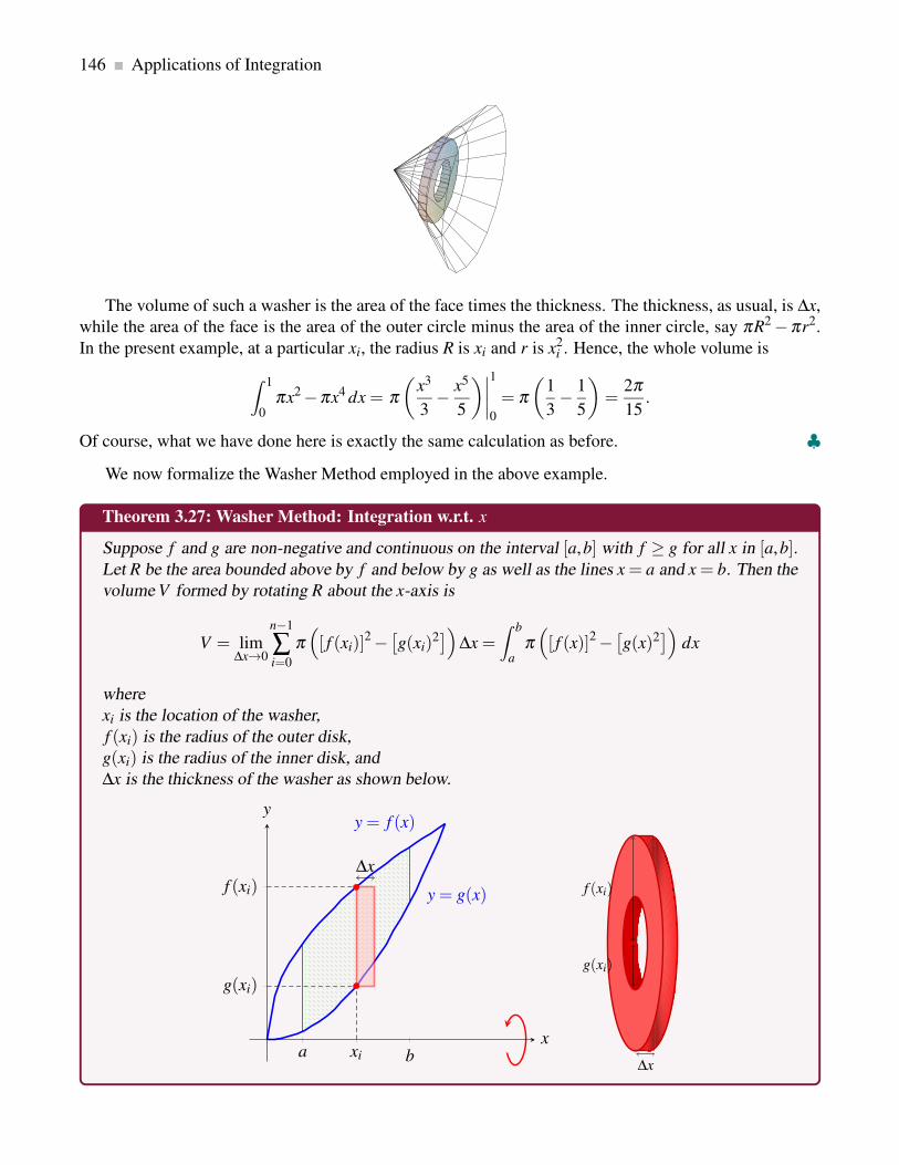
146 Applications of Integration
The volume of such a washer is the area of the face times the thickness. The thickness, as usual, is ∆x,
while the area of the face is the area of the outer circle minus the area of the inner circle, say πR2 −πr2.
In the present example, at a particular xi, the radius R is xi and r is x2i . Hence, the whole volume is
∫ 1
0πx2 −πx4 dx = π
(
x3
3− x5
5
)∣
∣
∣
∣
1
0
= π
(
1
3− 1
5
)
=2π
15.
Of course, what we have done here is exactly the same calculation as before. ♣We now formalize the Washer Method employed in the above example.
Theorem 3.27: Washer Method: Integration w.r.t. x
Suppose f and g are non-negative and continuous on the interval [a,b] with f ≥ g for all x in [a,b].Let R be the area bounded above by f and below by g as well as the lines x = a and x = b. Then the
volume V formed by rotating R about the x-axis is
V = lim∆x→0
n−1
∑i=0
π(
[ f (xi)]2 −[
g(xi)2]
)
∆x =
∫ b
aπ(
[ f (x)]2 −[
g(x)2]
)
dx
where
xi is the location of the washer,
f (xi) is the radius of the outer disk,
g(xi) is the radius of the inner disk, and
∆x is the thickness of the washer as shown below.
y = f (x)
y = g(x)
∆x
a xi b
g(xi)
f (xi)
x
y
f (xi)
g(xi)
∆x

3.3. Volume of Revolution: Disk Method 147
Note: The most common mistake in the Washer Method is to write ( f (x)− g(x))2 rather than f (x)2 −g(x)2.
We now present one more example that uses the Washer Method.
Example 3.28: Washer Method
Find the volume of the object generated when the area between g(x) = x2−x and f (x) = x is rotated
about the line y = 3.
Solution. The area between the two curves is graphed below to the left, noting the intersection points (0,0)and (2,2):
y = g(x)
y = f (x)
∆x
r
R
2
2
3
x
y
R
r
∆x
From the graph, we see that the inner radius must be r = 3− f (x) = 3− x, and the outer radius must be
R = 3−g(x) = 3− x2 + x. Therefore, the volume of the object is
V =
∫ 2
0π(
[
3− x2 + x]2 − [3− x]2
)
dx
=∫ 2
0π(
x4 −2x3 −6x2 +12x)
dx
= π
[
x5
5− x4
2−2x3 +6x2
]2
0
=32π
5.
♣
3.3.4. Disk and Washer Methods: Integration w.r.t. y
We have already seen in Section 3.1 that sometimes a curve is described as a function of y, namely x= g(y),and so the area of the region under the curve g over an interval [c,d] as shown to the left of Figure 3.13
can be rotated about the y-axis to generate a solid of revolution as indicated to the right in Figure 3.13.

148 Applications of Integration
c
d
x = g(y)
x
y
Figure 3.13: Area under a curve x = g(y).
We are readily convinced that the volume of such a solid of revolution can be calculated in a similar
manner as those discussed earlier, which is summarized in the following theorem.
Theorem 3.29: Disk Method: Integration w.r.t. y
Suppose g is non-negative and continuous on the interval [c,d]. Then the volume V formed by
rotating the area under the curve of g about the y-axis is
V = lim∆y→0
n−1
∑i=0
π [g(yi)]2 ∆y =
∫ b
aπ [g(y)]2 dy.
where
yi is the location of the disk,
g(yi) is the radius of the disk, and
∆y is the thickness of the disk as shown below.
g(yi)
c
yi
d
x = g(y)
∆y
x
y
g(yi)
∆y
Note: Either of the variations 1 and 2 described below will most likely create disks with holes in the solid

3.3. Volume of Revolution: Disk Method 149
of revolution, and so we would have to apply the Washer Method.
1. Again, we could rotate the area of any region around an axis of rotation, including the area of a
region bounded to the right by a function x = f (y) and to the left by a function x = g(y) on an
interval y ∈ [c,d].
2. The axis of rotation can be any axis parallel to the y-axis for this method to work.
We now provide an example of the Disk Method, where we integrate with respect to y.
Example 3.30: Disk Method
Find the volume of the object generated when the area between the curve f (x) = x2 and the line
y = 1 in the first quadrant is rotated about the y-axis.
Solution. The area between y = f (x) and y = 1 is shown below to the right. We notice that the two curves
intersect at (1,1), and that this area is contained between the two curves and the y-axis.
1
1
y = f (x)
∆y
x
y
1
1
x
y
We now solve for x as a function of y:
y = x2 =⇒ x =±√y,
and since we want the region in the first quadrant, we take x =√
y. The desired volume is found by
integrating
V = π
∫ 1
0(√
y)2 dy
= π
∫ 1
0ydy
=πy2
2
∣
∣
∣
∣
1
0
=π
2.

150 Applications of Integration
♣
Similar to the Washer Method when integrating with respect to x, we can also define the Washer
Method when we integrate with respect to y:
Theorem 3.31: Washer Method: Integration w.r.t. y
Suppose f and g are non-negative and continuous on the interval [c,d] with f ≥ g for all y in [c,d].Let R be the area bounded to the right by f and to the left by g as well as the lines y = c and y = d.
Then the volume V formed by rotating R about the y-axis is
V = lim∆y→0
n−1
∑i=0
π(
[ f (yi)]2 −[
g(yi)2]
)
∆y =∫ d
cπ(
[ f (y)]2 −[
g(y)2]
)
dy
where
yi is the location of the washer,
f (yi) is the radius of the outer disk,
g(yi) is the radius of the inner disk, and
∆y is the thickness of the washer as shown below.
g(yi) f (yi)
c
yi
d
x = g(y)
x = f (y)
∆y
x
y
f (yi)g(yi)
∆y
3.3.5. Summary
There are many different scenarios in which Disk and Washer Methods can be employed, which are not
discussed here; however, we provide a general guideline.

3.3. Volume of Revolution: Disk Method 151
Guideline for Disk and Washer Methods
The following steps outline how to employ the Disk or Washer Method.
1. Graph the bounded region.
2. Construct an arbitrary cross-section perpendicular to the axis of rotation.
3. Identify the radius (disk) or radii (washer).
4. Determine the thickness of the disk or washer.
5. Set up the definite integral by making sure you are computing the volume of the constructed
cross-section.
Exercises for Section 3.3
Exercise 3.3.1 Use the method from Section 3.3.1 to find each volume.
(a) The base of a tetrahedron (a triangular pyramid) of height h is an equilateral triangle of side s. Its
cross-sections perpendicular to an altitude are equilateral triangles. Express its volume V as an in-
tegral, and find a formula for V in terms of h and s. Verify that your answer is (1/3)(area of base)(height).
(b) The base of a solid is the region between f (x) = cosx and g(x) =−cosx, −π/2 ≤ x ≤ π/2, and its
cross-sections perpendicular to the x-axis are squares. Find the volume of the solid.
Exercise 3.3.2 Find the volume of the solid generated by revolving the shaded region about the given axis.
(a) About the x-axis:
2x+ y = 2
1
2
x
y

152 Applications of Integration
(b) About the y-axis:
x = 5y2
5
2
x
y
(c) About the y-axis:
1
1
x =√
y
x
y
(d) About the x-axis:
π4
π2
12
y = sin(x)cos(x)
x
y
Exercise 3.3.3 Find the volume of the solid generated by revolving the given bounded region about the
x-axis.
(a) y = x2, y = 1,x = 2
(b) y = x3, y = 0, x = 1
(c) y =√
4− x2, y = 0
(d) y =√
sinx, 0 ≤ x ≤ π/2
(e) y = e−x, y = 0, x = 2
(f) x+ y = 2, y = 0, x = 0
(g) y = x− x2, y = 0, x = 0
(h) y =√
sinx, x = 0

3.3. Volume of Revolution: Disk Method 153
Exercise 3.3.4 Find the volume of the solid generated by revolving the given bounded region about the
y-axis.
(a) x = y2, x = 0, y =−1, y = 1
(b) x = y3/2, x = 0, y = 4
(c) x =√
sin(2y), 0 ≤ y ≤ π/2, x = 0
(d) x =√
cos(2y), 0 ≤ y ≤ π/2, x = 0
Exercise 3.3.5 Find the volume of the solid generated by revolving the shaded region about the given axis.
(a) The x-axis:
y = 2√
cos(x)
y = 2
π2
x
y
(b) The y-axis:
x = sin(y)
1
π2
x
y
Exercise 3.3.6 Find the volume of the solid generated by revolving the given bounded region about the
x-axis.
(a) y = x,y = 2,x = 0
(b) y = 3√
x,y = 3,x = 0
(c) y = x2 +1,y+ x = 3
(d) y = 9− x2,y = 3− x
Exercise 3.3.7 The equation x2/9+ y2/4 = 1 describes an ellipse. Find the volume of the solid obtained
by rotating the ellipse around the x-axis and also around the y-axis. These solids are called ellipsoids; one
is vaguely rugby-ball shaped, one is sort of flying-saucer shaped, or perhaps squished-beach-ball-shaped.
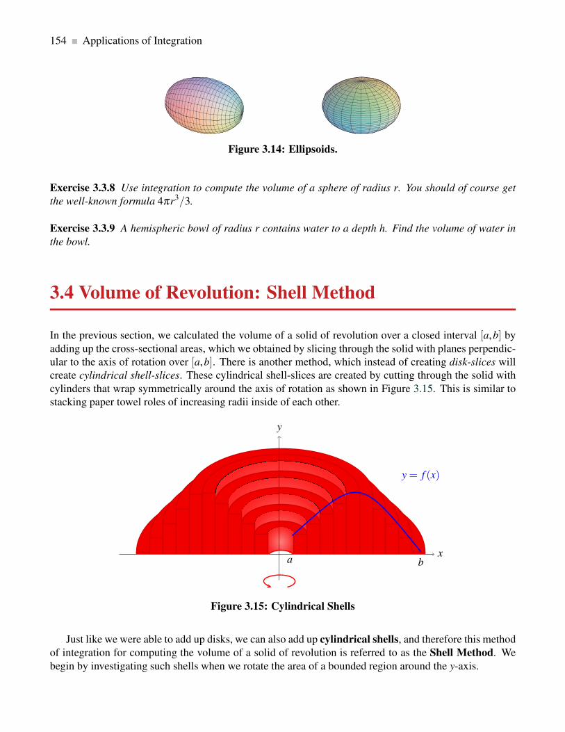
154 Applications of Integration
Figure 3.14: Ellipsoids.
Exercise 3.3.8 Use integration to compute the volume of a sphere of radius r. You should of course get
the well-known formula 4πr3/3.
Exercise 3.3.9 A hemispheric bowl of radius r contains water to a depth h. Find the volume of water in
the bowl.
3.4 Volume of Revolution: Shell Method
In the previous section, we calculated the volume of a solid of revolution over a closed interval [a,b] by
adding up the cross-sectional areas, which we obtained by slicing through the solid with planes perpendic-
ular to the axis of rotation over [a,b]. There is another method, which instead of creating disk-slices will
create cylindrical shell-slices. These cylindrical shell-slices are created by cutting through the solid with
cylinders that wrap symmetrically around the axis of rotation as shown in Figure 3.15. This is similar to
stacking paper towel roles of increasing radii inside of each other.
y
xa b
y = f (x)
Figure 3.15: Cylindrical Shells
Just like we were able to add up disks, we can also add up cylindrical shells, and therefore this method
of integration for computing the volume of a solid of revolution is referred to as the Shell Method. We
begin by investigating such shells when we rotate the area of a bounded region around the y-axis.

3.4. Volume of Revolution: Shell Method 155
3.4.1. Shell Method: Integration w.r.t. x
Suppose the region bounded by f (x) =√
x−1+ 2 with x ∈ [1,5] is rotated around the y-axis as shown
below to the right. It is possible, but inconvenient, to compute the volume of the resulting solid by the
Washer Method we have used so far. The problem is that there are two “kinds” of typical washers: Those
that go from the curve f to the line x = 5 and those that sit between the lines x = 1 and x = 5 as shown
below to the left.
1 5
2
4y = f (x)
x
y
To compute the volume using this approach, we need to break the problem into two parts and compute
two integrals:
V =∫ 2
0π(52−12)dy+
∫ 4
2π[
52 −(
(y−2)2 +1)2]
dy
=∫ 2
024π dy+
∫ 4
2π(
−y4 +8y3 −26y2 +40y)
dy
= 24πy
∣
∣
∣
∣
2
0
+π
[
−y5
5+2y4 − 26y3
3+20y2
]4
2
= 844
15π
If instead we slice through the solid of revolution parallel to the axis of rotation using cylindrical shells
with increasing radii over the interval [1,5] along the x-axis, then any of the cylindrical shells has height f
as shown below.

156 Applications of Integration
1 xi 5
2
4y = f (x)
x
y
Note that “washers” are related to the area of a circle, πr2, whereas “shells” are related to the surface
area of an open cylinder, 2πrh. If we add up the volume of such thin shells we will get an approximation
to the true volume. What is the volume of such a shell? Consider the shell at xi. Imagine that we cut the
shell vertically in one place and “unroll” the surface of the cylindrical shell into a thin, flat sheet, as shown
below.
y
xxi
h
r∆x
h
∆x2πr
This sheet will be almost a rectangular prism that is ∆x thick, h high, and 2πr wide (the circumference
of the cylindrical shell). In terms of xi, notice that h is the height of f , and that the radius r is precisely
xi. The volume of one cylindrical shell will then be approximately the volume of a rectangular prism with
these dimensions: 2πxi f (xi)∆x. If we add these up and take the limit as usual, we get the integral
V =
∫ 5
12πx f (x)dx =
∫ 5
12πx
(√x−1+2
)
dx.
Now use substitution to evaluate the integral:
u = x−1, x = u+1, du = dx, u(1) = 0, u(5) = 4.
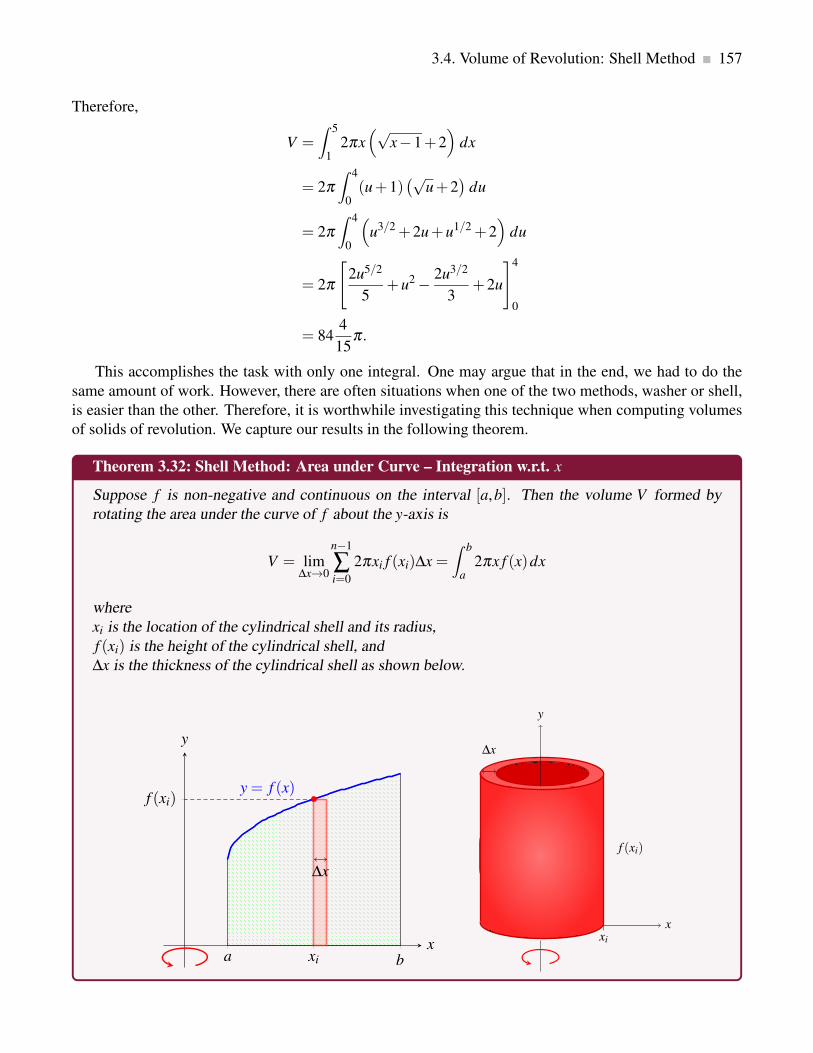
3.4. Volume of Revolution: Shell Method 157
Therefore,
V =
∫ 5
12πx
(√x−1+2
)
dx
= 2π
∫ 4
0(u+1)
(√u+2
)
du
= 2π
∫ 4
0
(
u3/2 +2u+u1/2 +2)
du
= 2π
[
2u5/2
5+u2 − 2u3/2
3+2u
]4
0
= 844
15π .
This accomplishes the task with only one integral. One may argue that in the end, we had to do the
same amount of work. However, there are often situations when one of the two methods, washer or shell,
is easier than the other. Therefore, it is worthwhile investigating this technique when computing volumes
of solids of revolution. We capture our results in the following theorem.
Theorem 3.32: Shell Method: Area under Curve – Integration w.r.t. x
Suppose f is non-negative and continuous on the interval [a,b]. Then the volume V formed by
rotating the area under the curve of f about the y-axis is
V = lim∆x→0
n−1
∑i=0
2πxi f (xi)∆x =
∫ b
a2πx f (x)dx
where
xi is the location of the cylindrical shell and its radius,
f (xi) is the height of the cylindrical shell, and
∆x is the thickness of the cylindrical shell as shown below.
a xi b
f (xi)y = f (x)
∆x
x
y
y
xxi
f (xi)
∆x

158 Applications of Integration
We now provide one example of the Shell Method.
Example 3.33: Shell Method – Integration w.r.t. x
Suppose the area below the curve f (x) = x+1 for all x in [0,3] is rotated about the y-axis. Find the
volume using the Shell Method.
Solution. We begin by graphing f on the interval [0,3] and identify an arbitrary cylindrical shell as shown
below.
xi 3
f (xi)
y = f (x)
∆x
x
y
y
xxi
f (xi)
∆x
Then the volume is given by
V =∫ 3
02πx f (x)dx =
∫ 3
02πx(x+1)dx
= 2π
∫ 3
0(x2 + x)dx = 2π
[
x3
3+
x2
2
]3
0
= 27π .
♣
Note:
1. Once again, we can rotate the area of any region around an axis of rotation, including the area of
a region bounded above by a function y = f (x) and below by a function y = g(x) on an interval
x ∈ [a,b] as we will investigate next.
2. The axis of rotation can be any axis parallel to the y-axis for this method to work. Consider again
the region bounded by the function f (x) =√
x−1+2 with x ∈ [1,5], but let’s also include a second
bound, namely the function g(x) = 14(x−1)2. Algebra shows us that f > g on x ∈ [1,5]. We want to
compute the volume of the solid obtained by rotating the bounded region about the y-axis. We begin
by graphing the region and remind ourselves that the given region is the difference of two regions
as shown below:

3.4. Volume of Revolution: Shell Method 159
1 5
2
4 y = f (x)
x
y
1 5
2
4
y = g(x)
x
y
1 5
2
4 y = f (x)
y = g(x)
x
y
The above figure shows us that the volume of the solid of revolution obtained from rotating the
given region is simply the difference between the volumes of the two solids of revolution that are
created from rotating the area under the curve of f and the area under the curve of g respectively.
An arbitrary cylindrical shell must therefore have height f (xi)−g(xi) as shown below.
1 xi 5
g(xi)
2
f (xi)
4y = f (x)
y = g(x)
f (xi)−g(xi)∆x
x
y
Therefore, the volume is given by
V =
∫ 5
12πx [ f (x)−g(x)] dx =
∫ 5
12πx
[√x−1+2− (x−1)2
4
]
dx =208π
5
We capture our result in the following theorem.

160 Applications of Integration
Theorem 3.34: Shell Method: Area between Curves – Integration w.r.t. x
Suppose f and g are non-negative and continuous on the interval [a,b] with f ≥ g for all x in [a,b].Let R be the area bounded above by f and below by g as well as the lines x = a and x = b. Then the
volume V formed by rotating R about the y-axis is
V = lim∆x→0
n−1
∑i=0
2πxi [ f (xi)−g(xi)] ∆x =∫ b
a2πx [ f (x)−g(x)] dx
where
xi is the location of the cylindrical shell and its radius,
f (xi)−g(xi) is the height of the cylindrical shell, and
∆x is the thickness of the cylindrical shell as shown below.
a xi b
g(xi)
f (xi)y = f (x)
y = g(x)
∆x
x
yy
xxi
f (xi)−g(xi)
∆x
We now provide one more example of such a region bounded below and above by two functions f and
g respectively.
Example 3.35: Shell Method – Integration w.r.t x
Suppose the region between f (x) = x+1 and g(x) = (x−1)2 is rotated around the y-axis. Find the
volume using the Shell Method.
Solution. We begin by finding the intersection points of the two functions f and g:
f (x) = g(x)
x+1 = (x−1)2
0 = x2 −3x = x(x−3)
and so x = 0 and x = 3 are the intersection points. We now use this information to graph f and g on the
interval [0,3] and identify an arbitrary cylindrical shell as shown below.

3.4. Volume of Revolution: Shell Method 161
xi 3
g(xi)
f (xi)
4
y = f (x)
y = g(x)∆x
x
y
Then the volume is computed as follows:
V =
∫ 3
02πx [ f (x)−g(x)] dx
=
∫ 3
02πx
[
(x+1)− (x−1)2]
dx
= 2π
∫ 3
0(3x2 − x3)dx
= 2π
[
x3 − x4
4
]3
0
=27
2π
♣
3.4.2. Shell Method: Integration w.r.t. y
So far, we have discussed three main manners of generating a solid of revolution and how to compute its
volume, which are listed below. Remember that the Washer Method is replaced by the Disk Method when
the lower or left curve is described by the x-axis or the y-axis respectively.
• Rotating an area that is bounded above and below by functions of x as well as lines x = a and x = b
around the x-axis, and then using the Washer Method for volume-computation.
• Rotating an area that is bounded right and left by functions of y as well as lines y = c and y = d
around the y-axis, and then using the Washer Method for volume-computation.
• Rotating an area that is bounded above and below by functions of x as well as lines x = a and x = b
around the y-axis, and then using the Shell Method for volume-computation.
There is only one case left:

162 Applications of Integration
• Rotating an area that is bounded right and left by functions of y as well as lines y = c and y = d
around the y-axis, and then using the Shell Method for volume-computation.
We are readily convinced that the volume of such a solid of revolution can be calculated using a Shell
Method similar in manner as the one discussed earlier, which is summarized in the following theorem.
Theorem 3.36: Shell Method: Area between Curves – Integration w.r.t. y
Suppose f and g are non-negative and continuous on the interval [c,d] with f ≥ g for all y in [c,d].Let R be the area bounded right by f and left by g as well as the lines y = c and y = d. Then the
volume V formed by rotating R about the x-axis is
V = lim∆y→0
n−1
∑i=0
2πyi [ f (yi)−g(yi)]∆y =
∫ d
c2πy [ f (y)−g(y)] dy
where
yi is the location of the cylindrical shell and its radius,
f (yi)−g(yi) is the height of the cylindrical shell, and
∆y is the thickness of the cylindrical shell as shown below.
g(yi) f (yi)
c
yi
d
x = g(y)
x = f (y)
∆y
x
y
x
f (yi)−g(yi)
∆y
We provide one example to exemplify this method as well.
Example 3.37:
Suppose the area under y = −x2 + 1 is rotated around the x-axis. Find the volume of the solid of
rotation using
(a) the Disk Method; and
(b) the Shell Method.
Solution.

3.4. Volume of Revolution: Shell Method 163
(a) We begin by graphing the area and indicate one arbitrary disk:
y =−x2 +1
∆x
-1 xi 1
yi
1
x
y
yi
∆x
Therefore, the volume is given by
V =∫ 1
−1πy2 dx =
∫ 1
−1π(
1− x2)2
dx
= 2π
∫ 1
0
(
x4 −2x2 +1)
dx = 2π
[
x5
5− 2x3
3+ x
]1
0
=16
15π
(b) We again begin by graphing the area and indicate one arbitrary cylindrical shell:
y =−x2 +1∆y
-1 xi 1
yi
1
x
y
x
2xi
∆y
First, we have to express x in terms of y:
y = 1− x2 =⇒ x =±√
1− y
Therefore, the volume is computed with
V =∫ 1
02πy(2x)dy = 4π
∫ 1
0y√
1− ydy.

164 Applications of Integration
Now we use substitution
u = 1− y, y = 1−u, du =−dy, u(0) = 1, u(1) = 0
and get
V = 4π
∫ 1
0y√
1− ydy = 4π
∫ 0
1(1−u)
√u(−du) = 4π
∫ 1
0
(
u1/2 −u3/2)
du
= 4π
[
2u3/2
3− 2u5/2
5
]1
0
=16
15π
♣
3.4.3. Summary
There are many different scenarios in which the Shell Method can be employed, which are not discussed
here; however, we provide a general guideline.
Guideline for Shell Method
The following steps outline how to employ the Shell Method.
1. Graph the bounded region.
2. Construct an arbitrary cylindrical shell parallel to the axis of rotation.
3. Identify the radius and height of the cylindrical shell.
4. Determine the thickness of the cylindrical shell.
5. Set up the definite integral by making sure you are computing the volume of the constructed
cylindrical shell.
Exercises for Section 3.4
Exercise 3.4.1 Use Shell Method to find the volumes of the solids generated by revolving the shaded
region about the indicated axis.
(a) The y-axis:

3.4. Volume of Revolution: Shell Method 165
2
1
5y = 1+ x2
x
y
(b) The y-axis:
1
1
2y = 2− x2
x
y
(c) The x-axis:
1 2
1
x = y2 +1
x
y
(d) The x-axis:

166 Applications of Integration
4
2
x = 4− y2
x
y
Exercise 3.4.2 Use Shell Method to find the volumes of the solids generated by revolving the given
bounded regions about the y-axis.
(a) y = 2x, y =−x, x = 1
(b) y = x, y = 2x, x = 2
(c) y = x2, y = x+2, x ≥ 0
(d) y = 1− x2, x2, x ≥ 0
(e) y =√
x, x−1, x = 0
(f) y = 1x , x = 2, x = 3, y = 0
Exercise 3.4.3 Use Shell Method to find the volumes of the solids generated by revolving the given
bounded regions about the x-axis.
(a) x = 2√
y, x =−y, y = 4
(b) x = y2, x = y, y ≥ 0
(c) x = y− y2/4, x = 0
(d) x = y− y2/4, x = y/2
(e) y = |x|, y = 2
(f) y = x+1, y = 2x
Exercise 3.4.4 Let R be the region of the x-y-plane bounded below by the curve y =√
x, and above by the
line y = 3. Find the volume of the solid obtained by rotating R around
(a) the x-axis;
(b) the line y = 3;
(c) the y-axis, and
(d) the line x = 9.
Exercise 3.4.5 Let S be the region of the x-y-plane bounded above by the curve x3y = 64, below by the
line y = 1, on the left by the line x = 2, and on the right by the line x = 4. Find the volume of the solid
obtained by rotating S around

3.4. Volume of Revolution: Shell Method 167
(a) the x-axis;
(b) the line y = 1;
(c) the y-axis, and
(d) the line x = 2.

4. Multiple Integration
4.1 Functions of Several Variables
Recall that a function f : R → R maps a single real value x to a single real value y. Such a function is
referred to as a single-variable function and can be readily visualized in a two-dimensional coordinate
system: above (or below) each point x on the x-axis we graph the point y, where of course y = f (x).By now, you have seen the graphs of many such functions. We now extend this visualization process to
multi-variable functions, also referred to as functions of several variables.
In single-variable calculus we were concerned with functions that map the real numbers R to R, some-
times called “real functions of one variable”, meaning the “input” is a single real number and the “output”
is likewise a single real number. Now we turn to functions of several variables, where several input vari-
ables are mapped to one value: functions f : Rn → R. We will deal primarily with n = 2 and to a lesser
extent n = 3; in fact many of the techniques we discuss can be applied to larger values of n as well.
A function f : R2 → R maps a pair of values (x,y) to a single real number. The three-dimensional
coordinate system is a convenient way to visualize such functions: above (or below) each point (x,y) in
the x-y-plane we graph the point (x,y,z), where then z = f (x,y). In other words, in interpreting the graph
of a function f (x,y), one often thinks of the value z = f (x,y) of the function at the point (x,y) as the
height of the point (x,y,z) on the graph of f . If f (x,y)> 0, then the point (x,y,z) is f (x,y) units above the
x-y-plane; if f (x,y) < 0, then the point (x,y,z) is | f (x,y)| units below the x-y-plane.
In general, it is quite difficult to draw the graph of a function of two variables. But techniques have
been developed that enable us to generate such graphs with minimum effort, using a computer. Still, it
is valuable to be able to visualize relatively simple surfaces without such aids. It is often a good idea to
examine the function on restricted subsets of the plane, especially lines. It can also be useful to identify
those points (x,y) that share a common z-value.
Before we introduce some special and some general three-dimensional graphs and their equations, let
us first consider the domain of functions in two variables.
The variables x and y are called independent variables, and the variable z, which is dependent on the
values of x and y, is referred to as a dependent variable. As indicated already, the number z = f (x,y) is
called the value of f at the point (x,y). Unless specified otherwise, the domain of the function f will be
taken to be the largest possible set for which the rule defining f is meaningful. We will demonstrate this
with several examples.
168

4.1. Functions of Several Variables 169
Example 4.1: Domain of Two-Variable Functions
Find the domain of each of the following functions.
(a) f (x,y) =√
1− x2 − y2.
(b) g(x,y) =1
√
1− x2 − y2.
(c) h(x,y) =1
y− x2.
Solution.
(a) The domain of f is the set of points (x,y) such that 1−x2 −y2 ≥ 0. We recognize x2 +y2 = 1 as the
equation of a circle of radius 1 centred at the origin, and so the domain of f consists of all points
which lie on or inside this circle (see below).
(b) We now require that 1− x2 − y2 > 0. The domain of g therefore contains all points (x,y) such that
x2 + y2 < 1; that is, all points which lie strictly inside the unit circle (see below).
(c) We see that h(x,y) is undefined for x = y2. The domain of h therefore consists of all points in the
x-y-plane except those which satisfy y =±√x (see below).
−1 1
−1
1
x
y
(a) Domain of f shown in grey.
−1 1
−1
1
x
y
(b) Domain of g shown in grey.
x
y
(c) Domain of h shown in grey.
♣

170 Multiple Integration
Example 4.2: Domain of Two-Variable Functions
A manufacturer produces a model X and a model Y, and determines that the unit prices of these two
products are related. Let qx be the weekly quantity demanded of model X, and let qy be the weekly
quantity demanded of model Y. The unit price of model X is found to be
px = 500−qx −1
3qy,
and the unit price of model Y is found to be
py = 200− 1
3qx −
1
5qy.
(a) Determine the revenue function R(qx,qy).
(b) Sketch the domain of R.
Solution.
(a) Selling qx units of model X yields a revenue of qx px dollars per week, and selling qy units of model
Y yields a revenue of qypy dollars per week. We therefore construct the revenue function R as
R(qx,qy) = qxpx +qypy
= qx
(
500−qx −1
3qy
)
+qy
(
200− 1
3qx −
1
5qy
)
=1
15
(
−15q2x −10qxqy +7500qx −3q2
y +3000qy
)
,
dollars per week.
(b) The domain of R is all points (qx,qy) in the plane such that qx,qy,px and py ≥ 0. That is, where
qx ≥ 0,
qy ≥ 0,
500−qx− 13qy ≥ 0 ⇐⇒ qy ≤ 1500−3qx
200− 13qx − 1
5qy ≥ 0 ⇐⇒ qy ≤ 1000− 53qx.
We find the domain by graphing the two lines given by px = 0 and py = 0 in the first quadrant of
the qx-qy-plane. The domain of R is the region which is bounded by the lines px = 0, py = 0, qx = 0
and qy = 0 for which the desired inequality holds. The final solution is given by the shaded region
(including the boundary) in the figure below.

4.1. Functions of Several Variables 171
py = 0
px = 0
200 400
1000
2000
qx
qy
♣
Let us now consider some functions that we can describe and graph with the knowledge we have
attained so far.
Example 4.3: Plane
Describe and graph the function f (x,y) = 3x+4y−5.
Solution.
We first write this as z = 3x + 4y− 5 and then 3x + 4y− z = 5, which is the equation of a plane.
However, we can also determine that this equation represents a plane from the following analysis: If we
hold x constant, then the equation simplifies to that of a straight line in the y-z-plane. Generally speaking,
if we choose any point on the graph of f , for example from f (0,0) = −5, this function grows linearly in
every direction in the same way that a linear function behaves as can be seen below.
To graph the plane, we alternately let x, then y, then z be equal to zero, which leads to a linear equation
in the y-z-, x-z-, and x-y-planes respectively. These lines represent the intersection of the functions’ graph
with each of the coordinate planes in the three-dimensional coordinate system and form part of the plane
surface as shown below.
−1 −0.5 00.5 1 −1
0
1−10
0
x
y
f(x,
y)

172 Multiple Integration
♣
Example 4.4: Sphere
Describe and graph the equation x2 + y2 + z2 = 4.
Solution. The equation x2 + y2 + z2 = 4 represents a sphere of radius 2 and centre (0,0,0) as shown
below. We cannot write this in the form z = f (x,y), since for each x and y in the disk x2 + y2 < 4 there
are two corresponding points on the sphere, namely one above and one below this point (x,y). As with
the equation of a circle, we can resolve this equation into two functions, f1(x,y) =√
4− x2 − y2 and
f2(x,y) =−√
4− x2 − y2, representing the upper and lower hemispheres, respectively. Each of these is an
example of a function with a restricted domain: only certain values of x and y make sense (namely, those
for which x2 + y2 ≤ 4) and the graphs of these functions are limited to a small region of the plane.
x
yz
♣
Example 4.5: Square Root
Describe and graph the function f (x,y) =√
x+√
y.
Solution. This function is defined only when both x and y are non-negative. When y = 0 we get f (x,y) =√x, the familiar square root function in the x-z-plane, and when x = 0 we get the same curve in the y-z-
plane. Generally speaking, we see that starting from f (0,0) = 0 this function gets larger in every direction
in roughly the same way that the square root function gets larger. For example, if we restrict attention to
the line x = y, we get f (x,y) = 2√
x and along the line y = 2x we have f (x,y) =√
x+√
2x = (1+√
2)√
x
(see graph below).

4.1. Functions of Several Variables 173
10.0
7.5
5.000.0 y
2.5
1
2.55.0
x
2
7.50.0
10.0
3
4
5
6
♣
Example 4.6: Elliptic Paraboloid
Describe and graph the function f (x,y) = x2 + y2.
Solution. When x = 0 this becomes f (y) = y2, a parabola in the y-z-plane; when y = 0 we get the “same”
parabola f (x) = x2 in the x-z-plane.
Finally, picking a value z = k, at what points does f (x,y) = k? This means x2 + y2 = k, which we
recognize as the equation of a circle of radius√
k, as seen in the graph below to the right. So the graph of
f (x,y) has parabolic cross-sections as shown in the graph below to the left, and the same height everywhere
on concentric circles with centre at the origin. This fits with what we have already discovered.
−30−3
−2−2
2
−1−1
4
00
6
11
8
2233
2
1
−1 2
−1
−2
0
0
−2
1
♣
As in this example, the points (x,y) such that f (x,y) = k form a curve, called a level curve of the
function. A graph of some level curves can give a good idea of the shape of the surface; it looks much like
a topographic map of the surface. By drawing the level curves corresponding to several admissible values
of k, we obtain a contour map. In the graph of Example 4.6 both the surface and its associated level
curves are shown. Note that, as with a topographic map, the heights corresponding to the level curves are
evenly spaced, so that where curves are closer together the surface is steeper.

174 Multiple Integration
Example 4.7: Level Curves
Sketch the level curves of the function z = f (x,y) = 4x2 − y corresponding to z =−2,−1,0,1,2.
Solution. We find the level curves of f by setting f (x,y) = z to be a constant. For z = −2,−1,0,1,2, we
find the equationsy = 4x2 +2
y = 4x2 +1
y = 4x2
y = 4x2 −1
y = 4x2 −2
and so each level curve is a parabola in the x-y-plane, where only the y-intercept changes. These level
curves are shown in the graph below to the left, and the graph of f (x,y) is shown to the right for reference.
−1 1
−3
3
k =-2
k =-1
k =0
k =1
k =2
x
y
(a) Level curves of f
−4 −2 0 2 4 −4−2
02
40
50
xy
z
(b) The graph of z = f (x,y)
♣
Example 4.8: Level Curves
Sketch the level curves of the function z = f (x,y) =√
x2 + y2 corresponding to z = 0,1,2,3.
Solution. For each level curve corresponding to z = c, we have
√
x2 + y2 = c =⇒ x2 + y2 = c2,
which is the equation of a circle centred at (0,0) of radius c. These level curves are drawn below in the
graph to the left. The graph of z = f (x,y) is provided to the right.

4.1. Functions of Several Variables 175
−1−2−3 1 2 3
−2
2
k = 0
k = 1
k = 2
k = 3
x
y
(a) Level curves of f
−4 −2 0 2 4 −5
0
50
2
4
xy
z
(b) The graph of z = f (x,y)
♣
Example 4.9: Home Mortgage Payments
The monthly payment for a condo that amortizes a loan of A dollars in t years when the interest rate
is r per year is given by
P = f (A,r, t) =Ar
12[
1−(
1+ r12
)−12t]
Find the monthly payment for a home mortgage of $240,000 to be amortized over 25 years when
the interest rate is 4% per year.
Solution. P is a function of three variables: A, r and t. To find the required monthly payments, we evaluate
P at the given values,
P = f (240000,0.04,25)
=240000(0.04)
12[
1−(
1+ 0.0412
)−12(25)]
≈ 1266.81.
Thus, the monthly payments would be about $1266.81. ♣
Functions f : Rn → R for n > 2 behave much like functions of two variables. The principal difficulty
with such functions is visualizing them, as they do not “fit” in the three dimensions we are familiar with.
For n = 3 variables there are various ways to interpret functions that make them easier to understand. For
example, f (x,y,z) could represent the temperature at the point (x,y,z), or the strength of a magnetic field.
Similar to considering level curves with two-variable functions, it is useful to consider those points at
which f (x1,x2, . . . ,xn) = k, where k is some constant for n-variable functions. This collection of points is
called a level set. For three variables, a level set is a surface, called a level surface.

176 Multiple Integration
Example 4.10: Level Surfaces
Suppose the temperature at (x,y,z) is T (x,y,z) = e−(x2+y2+z2). Describe the level surfaces.
Solution. This function has a maximum value of 1 at the origin, and tends to 0 in all directions. If k is
positive and at most 1, the set of points for which T (x,y,z) = k is those points satisfying x2 + y2 + z2 =− lnk, a sphere centred at the origin. The level surfaces are the concentric spheres centred at the origin.
♣
Exercises for Section 4.1
Exercise 4.1.1 Find the equations and describe the shapes of the cross-sections when x = 0, y = 0 and
x = y. Plot the surface with a three-dimensional graphing tool.
(a) f (x,y) = (x− y)2
(b) f (x,y) = |x|+ |y|
(c) f (x,y) = e−(x2+y2) sin(x2 + y2)
(d) f (x,y) = sin(x− y)
(e) f (x,y) = (x2 − y2)2
Exercise 4.1.2 Find the domain of each of the following functions:
(a) f (x,y) =√
9− x2 +√
y2 −4
(b) h(u,v) =√
2−u2 − v2
(c) f (x,y) =√
16− x2 −4y2
(d) f (x,y) = x+4y
(e) g(x,y,z) = x2 + y2 + z2
(f) f (x,y) = arcsin(x2 + y2 −2)
(g) h(u,v) =uv
u− v
(h) f (s, t) =√
s2 + t2
(i) g(r,s) =√
rs
(j) f (x,y) = e−xy
(k) h(x,y) = ln(x+ y−7)
Exercise 4.1.3 Below are two sets of level curves at a sequence of equally-spaced heights z. One is for a

4.1. Functions of Several Variables 177
cone, one is for a paraboloid. Which is which? Explain.
K2 K1 0 1 2
K2
K1
1
2
K2 K1 0 1 2
K2
K1
1
2
Exercise 4.1.4 Sketch the level curves of the function corresponding to the given values of z.
(a) f (x,y) = 3x+2y, z =−2,−1,0,1,2
(b) f (x,y) = x2 − y, z =−2,−1,0,1,2
(c) f (x,y) = 2y+ x2, z =−2,−1,0,1,2
(d) f (x,y) = 2xy, z =−4,−2,2,4
(e) f (x,y) =√
25− x2 − y2, z = 0,1,3,5
(f) f (x,y) = ey − x2, z = 1,2,3,4
Exercise 4.1.5 A clothing retailer sells casual and business jackets. Let qc denote the quantity of ca-
sual jackets demanded monthly and qb denote the quantity of business jackets demanded monthly. It is
determined that the unit price of casual jackets is approximately
pc = 100− 1
4qc −
1
7qb,
and that the unit price of business jackets is approximately
pb = 150− 1
10qc −
1
3qb
dollars, respectively.
(a) Determine the monthly revenue, R(qc,qb).
(b) Determine the domain of R.
Exercise 4.1.6 A certain manufacturer produces basic and enhanced versions of their product. Let qb
denote the quantity of basic units daily demanded and qe denote the quantity of enhanced units demanded
daily. It is determined that the unit price of the basic units is approximately
pb = 10−0.1qb −0.5qe,
and that the unit price of the enhanced units is approximately
pe = 30−0.4qb−qe
dollars, respectively.
(a) Determine the daily revenue, R(qb,qe).

178 Multiple Integration
(b) Determine the domain of R.
Exercise 4.1.7 We can calculate the outstanding principal on a loan at the end of i months by the formula
B(A,r, t, i) = A
(
(
1+ r12
)i −1(
1+ r12
)12t −1
)
0 ≤ i ≤ 12t
where A is the principal loan, r is the annual interest rate, and t is the amortization period in years.
Suppose the original amount borrowed is $100,000, and the interest rate charged by the bank is 3%. What
is the amount owed to the bank after 2 years if the loan is to be repaid in equal instalments over 25 years?
What is the amount owed after 20 years?
Exercise 4.1.8 In economics, the given optimal quantity Q of goods for a store to order is given by the
Wilson lot-size formula:
Q(C,N,H) =
√
2CN
H
where C is the cost of placing an order, N is the number of items the store sells per day, and H is the daily
holding cost for each item. What is the most economical quantity of winter tires to order if the store pays
$25 for placing an order, pays $2 for holding a tire per day, and expects to sell 60 tires a day?
4.2 Double Integrals: Volume and Average Value
Consider a surface f (x,y). In this section, we are interested in computing either the volume under f or
the average function value of f over a certain area in the x-y-plane. You might temporarily think of this
surface as representing physical topography—a hilly landscape, perhaps. What is the average height of
the surface (or average altitude of the landscape) over some region?
4.2.1. Volume and Average Value over a Rectangular Region
As with most such problems, we start by thinking about how we might approximate the answer. Suppose
the region is a rectangle, [a,b]× [c,d]. We can divide the rectangle into a grid, m subdivisions in one
direction and n in the other, as indicated in the 2D graph below, where m = 6 and n = 4. We pick x-values
x0, x1,. . . , xm−1 in each subdivision in the x-direction, and similarly in the y-direction. At each of the
points (xi,y j) in one of the smaller rectangles in the grid, we compute the height of the surface: f (xi,y j).Now the average of these heights should be (depending on the fineness of the grid) close to the average
height of the surface:
f (x0,y0)+ f (x1,y0)+ · · ·+ f (x0,y1)+ f (x1,y1)+ · · ·+ f (xm−1,yn−1)
mn
As both m and n go to infinity, we expect this approximation to converge to a fixed value, the actual
average height of the surface. For reasonably nice functions this does indeed happen.

4.2. Double Integrals: Volume and Average Value 179
c
y1
y2
y3
d
a x1 x2 x3 x4 x5 b
∆x
∆y
Using sigma notation, we can rewrite the approximation:
1
mn
n−1
∑i=0
m−1
∑j=0
f (x j,yi) =1
(b−a)(d− c)
n−1
∑i=0
m−1
∑j=0
f (x j,yi)b−a
m
d − c
n
=1
(b−a)(d− c)
n−1
∑i=0
m−1
∑j=0
f (x j,yi)∆x∆y.
The two parts of this product have useful meaning: (b− a)(d − c) is of course the area of the rectangle,
and the double sum adds up mn terms of the form f (x j,yi)∆x∆y, which is the height of the surface at a
point multiplied by the area of one of the small rectangles into which we have divided the large rectangle.
In short, each term f (x j,yi)∆x∆y is the volume of a tall, thin, rectangular box, and is approximately the
volume under the surface and above one of the small rectangles; see Figure 4.1. When we add all of these
up, we get an approximation to the volume under the surface and above the rectangle R = [a,b]× [c,d].When we take the limit as m and n go to infinity, the double sum becomes the actual volume under the
surface, which we divide by (b−a)(d− c) to get the average height.
12
31
20
1
2
x
y
z
(a) The surface z on [0.5,3.5]× [0.5,2.5]. (b) Approximating the volume under z.
Figure 4.1: The surface z = sin(xy)+ 65 .
Double sums like this come up in many applications, so in a way it is the most important part of this
example; dividing by (b−a)(d−c) is a simple extra step that allows the computation of an average. This

180 Multiple Integration
computation is independent of f being positive, and so as we did in the single variable case, we introduce
a special notation for the limit of such a double sum, which is referred to as the double integral of f over
the region R.
Definition 4.11: Double Integral over a Rectangular Region
Let f (x,y) be a continuous function defined over the rectangle R = [a,b]× [c,d], then the double
integral of f over R is denoted by
∫∫
Rf (x,y)dA =
∫∫
Rf (x,y)dxdy = lim
m→∞limn→∞
n−1
∑i=0
m−1
∑j=0
f (x j,yi)∆x∆y,
provided the limit exists.
Note: The notation dA indicates a small element of area, without specifying any particular order for the
variables x and y; it is shorter and more “generic” than writing dxdy.
We now capture our results from the earlier calculations using the notation of the double integral.
Theorem 4.12: Average Value of a Two-variable Function
Let f (x,y) be a continuous function defined over the rectangle R = [a,b]× [c,d], then the average
value favg of f over R is
favg =1
(b−a)(d− c)
∫∫
Rf (x,y)dA,
provided the double integral exists.
Theorem 4.13: Volume Below a Surface
Let f (x,y) be a continuous function defined over the rectangle R = [a,b]× [c,d], with f (x,y) ≥ 0,
then the volume V below the surface f is
V =
∫∫
Rf (x,y)dA,
provided the double integral exists.
Note: Just as with single-variable integration, this last theorem can be stated for more general functions
that can take on negative values, as long as we understand that V represents a signed volume.
4.2.2. Computing Double Integrals over Rectangular Regions
The next question, of course, is: How do we compute these double integrals? You might think that we will
need some two-dimensional version of the Fundamental Theorem of Calculus, but as it turns out we can
get away with just the single variable version, applied twice.

4.2. Double Integrals: Volume and Average Value 181
Going back to the double sum, we can rewrite it to emphasize a particular order in which we want to
add the terms:n−1
∑i=0
(
m−1
∑j=0
f (x j,yi)∆x
)
∆y.
In the sum in parentheses, only the value of x j is changing; yi is temporarily constant. As m goes to infinity,
this sum has the right form to turn into an integral:
limm→∞
m−1
∑j=0
f (x j,yi)∆x =
∫ b
af (x,yi)dx.
So after we take the limit as m goes to infinity, the sum is
n−1
∑i=0
(
∫ b
af (x,yi)dx
)
∆y.
Of course, for different values of yi this integral has different values; in other words, it is really a function
applied to yi:
G(y) =∫ b
af (x,y)dx.
If we substitute back into the sum we getn−1
∑i=0
G(yi)∆y.
This sum has a nice interpretation. The value G(yi) is the area of a cross section of the region under the
surface f (x,y), namely, when y = yi. The quantity G(yi)∆y can be interpreted as the volume of a solid
with face area G(yi) and thickness ∆y. Think of the surface f (x,y) as the top of a loaf of sliced bread.
Each slice has a cross-sectional area and a thickness; G(yi)∆y corresponds to the volume of a single slice
of bread. Adding these up approximates the total volume of the loaf. (This is very similar to the technique
we used to compute volumes in Section 3.3, except that there we need the cross-sections to be in some
way “the same”.) Figure 4.2 shows this “sliced loaf” approximation using the same surface as shown in
Figure 4.1. Nicely enough, this sum looks just like the sort of sum that turns into an integral, namely,
limn→∞
n−1
∑i=0
G(yi)∆y =∫ d
cG(y)dy
=∫ d
c
∫ b
af (x,y)dxdy.
Let’s be clear about what this means: we first will compute the inner integral, temporarily treating y as a
constant. We will do this by finding an antiderivative with respect to x, then substituting x = a and x = b
and subtracting, as usual. The result will be an expression with no x variable but some occurrences of y.
Then the outer integral will be an ordinary one-variable problem, with y as the variable.

182 Multiple Integration
Figure 4.2: Approximating the volume under a surface with slices.
Example 4.14: Average Height
Figure 4.1 shows the function sin(xy)+6/5 on [0.5,3.5]× [0.5,2.5]. Find the average height of this
surface.
Solution. The volume under this surface is
∫ 2.5
0.5
∫ 3.5
0.5sin(xy)+
6
5dxdy.
The inner integral is
∫ 3.5
0.5sin(xy)+
6
5dx =
−cos(xy)
y+
6x
5
∣
∣
∣
∣
3.5
0.5
=−cos(3.5y)
y+
cos(0.5y)
y+
18
5.
Unfortunately, this gives a function for which we can’t find a simple antiderivative. To complete the
problem we could use Sage or similar software to approximate the integral. Doing this gives a volume of
approximately 8.84, so the average height is approximately 8.84/6 ≈ 1.47. ♣
Because addition and multiplication are commutative and associative, we can rewrite the original dou-
ble sum:n−1
∑i=0
m−1
∑j=0
f (x j,yi)∆x∆y =m−1
∑j=0
n−1
∑i=0
f (x j,yi)∆y∆x.
Now if we repeat the development above, the inner sum turns into an integral:
limn→∞
n−1
∑i=0
f (x j,yi)∆y =
∫ d
cf (x j,y)dy,
and then the outer sum turns into an integral:
limm→∞
m−1
∑j=0
(
∫ d
cf (x j,y)dy
)
∆x =
∫ b
a
∫ d
cf (x,y)dydx.

4.2. Double Integrals: Volume and Average Value 183
In other words, we can compute the integrals in either order, first with respect to x then y, or vice versa.
Thinking of the loaf of bread, this corresponds to slicing the loaf in a direction perpendicular to the first.
We summarize our findings by providing a general guideline for how the double integral over a rect-
angle is computed.
Guideline for Computing a Double Integral over a Rectangle
Let f (x,y) be a continuous function defined over the rectangle R = [a,b]× [c,d]. Follow these steps
to evaluate the double integral
∫ d
c
∫ b
af (x,y)dxdy =
∫ b
a
∫ d
cf (x,y)dydx.
1. Choose the double integral,
∫ d
c
∫ b
af (x,y)dxdy or
∫ b
a
∫ d
cf (x,y)dydx.
2. Compute the inner integral:
(a) If
∫ b
af (x,y)dx, then temporarily treat y as a constant. Find an antiderivative with respect
to x, then evaluate over the integration bounds x = a and x = b.
(b) If
∫ d
cf (x,y)dy, then temporarily treat x as a constant. Find an antiderivative with respect
to y, then evaluate over the integration bounds y = c and y = d.
3. Compute the outer integral, which will be an ordinary one-variable integral of the form
∫ d
cG(y)dy or
∫ b
aG(x)dx.
We haven’t really proved that the value of a double integral is equal to the value of the corresponding
two single integrals in either order of integration, but provided the function is continuous, this is true. The
result is called Fubini’s Theorem, which we state here without proof.
Theorem 4.15: Fubini’s Theorem for Rectangular Regions of Integration
Let f (x,y) be a continuous function defined over the rectangle R = [a,b]× [c,d]. Then the order of
integration does not matter, and so
∫∫
Rf (x,y)dA =
∫ d
c
∫ b
af (x,y)dxdy =
∫ b
a
∫ d
cf (x,y)dydx.
We provide one example, where we compute the volume under a surface in two ways by switching the
order of integration.

184 Multiple Integration
Example 4.16: Compute Volume in Two Ways
We compute
∫∫
R1+(x−1)2 +4y2 dA, where R = [0,3]× [0,2], in two ways.
Solution. First,
∫ 3
0
∫ 2
01+(x−1)2 +4y2 dydx =
∫ 3
0y+(x−1)2y+
4
3y3
∣
∣
∣
∣
2
0
dx
=∫ 3
02+2(x−1)2 +
32
3dx
= 2x+2
3(x−1)3 +
32
3x
∣
∣
∣
∣
3
0
= 6+2
3·8+ 32
3·3− (0−1 · 2
3+0)
= 44.
In the other order:
∫ 2
0
∫ 3
01+(x−1)2 +4y2 dxdy =
∫ 2
0x+
(x−1)3
3+4y2x
∣
∣
∣
∣
3
0
dy
=
∫ 2
03+
8
3+12y2 +
1
3dy
= 3y+8
3y+4y3 +
1
3y
∣
∣
∣
∣
2
0
= 6+16
3+32+
2
3
= 44.
♣Note: In this example there is no particular reason to favor one direction over the other; in some cases,
one direction might be much easier than the other, so it’s usually worth considering the two different
possibilities.
4.2.3. Computing Double Integrals over any Region
Frequently we will be interested in a region that is not simply a rectangle. Let’s compute the volume under
the surface x+2y2 above the region described by 0 ≤ x ≤ 1 and 0 ≤ y ≤ x2, shown below.
0 10
1

4.2. Double Integrals: Volume and Average Value 185
In principle there is nothing more difficult about this problem. If we imagine the three-dimensional
region under the surface and above the parabolic region as an oddly shaped loaf of bread, we can still
slice it up, approximate the volume of each slice, and add these volumes up. For example, if we slice
perpendicular to the x-axis at xi, the thickness of a slice will be ∆x and the area of the slice will be
∫ x2i
0xi +2y2 dy.
When we add these up and take the limit as ∆x goes to 0, we get the double integral
∫ 1
0
∫ x2
0x+2y2 dydx =
∫ 1
0xy+
2
3y3
∣
∣
∣
∣
x2
0
dx
=
∫ 1
0x3 +
2
3x6 dx
=x4
4+
2
21x7
∣
∣
∣
∣
1
0
=1
4+
2
21=
29
84.
We could just as well slice the solid perpendicular to the y-axis, in which case we get
∫ 1
0
∫ 1
√yx+2y2 dxdy =
∫ 1
0
x2
2+2y2x
∣
∣
∣
∣
1
√y
dy
=∫ 1
0
1
2+2y2 − y
2−2y2√ydy
=y
2+
2
3y3 − y2
4− 4
7y7/2
∣
∣
∣
∣
1
0
=1
2+
2
3− 1
4− 4
7=
29
84.
What is the average height of the surface over this region? As before, it is the volume divided by the area
of the base, but now we need to use integration to compute the area of the base, since it is not a simple
rectangle. The area is∫ 1
0x2 dx =
1
3,
so the average height is29
84÷ 1
3=
29
28.
Although we have not proven that the order of integration can be switched, we nonetheless capture our
results and state the general version of Fubini’s Theorem without proof.

186 Multiple Integration
Theorem 4.17: Fubini’s Theorem for General Regions of Integration
Let f (x,y) be a continuous function defined over the region R.
1. If R is bounded by a ≤ x ≤ b, g1(x)≤ y ≤ g2(x), with g1 and g2 continuous on [a,b], then
∫∫
Rf (x,y)dA =
∫ b
a
∫ g2(x)
g1(x)f (x,y)dydx.
2. If R is bounded by c ≤ y ≤ d, h1(y)≤ x ≤ h2(y), with h1 and h2 continuous on [c,d], then
∫∫
Rf (x,y)dA =
∫ d
c
∫ h2(y)
h1(y)f (x,y)dxdy.
Note: Although Fubini’s Theorem tells us that the order of integration does not matter in a double integral,
the theorem does not tell us which of the double integrals is easier to compute. Experience through practice
allows us to decide whether to choose to set up a double integral with dxdy or dydx.
We explore the order of integration with one more example of a double integral.
Example 4.18: Volume of Region
Find the volume under the surface z =√
1− x2 and above the triangle formed by y = x, x = 1, and
the x-axis.
Solution. Let’s consider the two possible ways to set this up:∫ 1
0
∫ x
0
√
1− x2 dydx or
∫ 1
0
∫ 1
y
√
1− x2 dxdy.
Which appears easier? In the first, the first (inner) integral is easy, because we need an antiderivative with
respect to y, and the entire integrand√
1− x2 is constant with respect to y. Of course, the second integral
may be more difficult. In the second, the first integral is mildly unpleasant—a trig substitution. So let’s
try the first one, since the first step is easy, and see where that leaves us.∫ 1
0
∫ x
0
√
1− x2 dydx =∫ 1
0y√
1− x2∣
∣
∣
x
0dx =
∫ 1
0x√
1− x2 dx.
This is quite easy, since the substitution u = 1− x2 works:∫
x√
1− x2 dx =−1
2
∫ √udu =
1
3u3/2 =−1
3(1− x2)3/2.
Then∫ 1
0x√
1− x2 dx = −1
3(1− x2)3/2
∣
∣
∣
∣
1
0
=1
3.
This is a good example of how the order of integration can affect the complexity of the problem. In this
case it is possible to do the other order, but it is a bit messier. In some cases one order may lead to an
integral that is either difficult or impossible to evaluate; it’s usually worth considering both possibilities
before going very far. ♣

4.2. Double Integrals: Volume and Average Value 187
Exercises for Section 4.2
Exercise 4.2.1 Compute the following double integrals.
(a)
∫ 2
0
∫ 4
01+ xdydx
(b)
∫ 1
−1
∫ 2
0x+ ydydx
(c)
∫ 2
1
∫ y
0xydxdy
(d)
∫ 1
0
∫
√y
y2/2dxdy
(e)
∫ 2
1
∫ x
1
x2
y2dydx
(f)
∫ 1
0
∫ x2
0
y
exdydx
(g)
∫
√π/2
0
∫ x2
0xcosydydx
(h)
∫ π/2
0
∫ cosθ
0r2(cosθ − r)dr dθ
(i)
∫ 1
0
∫ 1
√y
√
x3 +1dxdy
(j)
∫ 1
0
∫ 1
y2
(k)
∫ 1
0
∫ 1
x2x√
1+ y2 dydx
(l)
∫ 1
0
∫ y
0
2√1− x2
dxdy
(m)
∫ 1
0
∫ 3
3yex2
dxdy
(n)
∫ 1
−1
∫ 1−x2
0x2 −√
ydydx
(o)
∫
√2/2
0
∫
√1−2x2
−√
1−2x2xdydx
Exercise 4.2.2 Determine the volume of the region that is bounded as follows:
(a) below z = 1− y and above the region −1 ≤ x ≤ 1, 0 ≤ y ≤ 1− x2
(b) bounded by z = x2 + y2 and z = 4
(c) in the first octant bounded by y2 = 4− x and y = 2z
(d) in the first octant bounded by y2 = 4x, 2x+ y = 4, z = y, and y = 0
(e) in the first octant bounded by x+ y+ z = 9, 2x+3y = 18, and x+3y = 9.
(f) in the first octant bounded by x2 + y2 = a2 and z = x+ y
(g) bounded by 4x2 + y2 = 4z and z = 2
(h) bounded by z = x2 + y2 and z = y
(i) under the surface z = xy and above the triangle with vertices (1,1,0), (4,1,0), (1,2,0)
(j) enclosed by y = x2, y = 4, z = x2, z = 0

188 Multiple Integration
Exercise 4.2.3 Evaluate
∫∫
x2 dA over the region in the first quadrant bounded by the hyperbola xy = 16
and the lines y = x, y = 0, and x = 8.
Exercise 4.2.4 A swimming pool is circular with a 40 meter diameter. The depth is constant along east-
west lines and increases linearly from 2 meters at the south end to 7 meters at the north end. Find the
volume of the pool.
Exercise 4.2.5 Find the average value of f (x,y) = ey√
x+ ey on the rectangle with vertices (0,0), (4,0),
(4,1) and (0,1).
Exercise 4.2.6 Reverse the order of integration on each of the following integrals
(a)
∫ 9
0
∫
√9−y
0f (x,y) dx dy
(b)
∫ 2
1
∫ lnx
0f (x,y) dy dx
(c)
∫ 1
0
∫ π/2
arcsinyf (x,y) dx dy
(d)
∫ 1
0
∫ 4
4xf (x,y) dy dx
(e)
∫ 3
0
∫
√9−y2
0f (x,y) dx dy
4.3 Triple Integrals: Volume and Average Value
It will come as no surprise that we can also do triple integrals—integrals over a three-dimensional region.
The simplest application allows us to compute volumes in an alternate way.
We follow the same method as we have done when we defined a single integral for functions of one
variable and a double integral for functions of two variables. Suppose that f (x,y,z) is a continuous function
on a closed bounded region S in space. If the boundaries of S are “relatively smooth”, then we can divide
the three-dimensional region into small rectangular boxes with dimensions ∆x×∆y×∆z and with volume
dV = ∆x∆y∆z. Then we add them all up and take the limit, to get an integral:∫∫∫
Sf (x,y,z)dV .
Note:
1. Fubini’s Theorem also holds for triple integrals, which means that the order of integration does not
matter and we can choose from setting up a triple integral with any of the following six choices for
the order of integration: dxdydz, dxdzdy, dydxdz, dydzdx, dzdxdy, and dzdydx. However, the
same word of caution holds here as well, as some orders may lead to a more readily computable
triple integral, while others may simply be too difficult to compute.
2. If the three-variable function f is the constant 1, then the triple integral
∫∫∫
SdV evaluates to the
volume of the closed bounded region S.

4.3. Triple Integrals: Volume and Average Value 189
3. If the three-variable function f is the constant 1 and S is bounded by constants, then we are simply
computing the volume of a rectangular box.
Example 4.19: Volume of a Box
Compute the volume of the box with opposite corners at (0,0,0) and (1,2,3).
Solution. We begin by drawing an outline of the rectangular box as shown below.
12
3
(1,2,3)
(0,0,0)
x
y
z
Since the faces of the rectangular box are parallel to the coordinate planes, we deduce that the integra-
tion bounds are given by
0 ≤ x ≤ 1, 0 ≤ y ≤ 2, 0 ≤ z ≤ 3.
Hence, the following triple integral computes the volume of the rectangular box:
∫ 1
0
∫ 2
0
∫ 3
0dzdydx =
∫ 1
0
∫ 2
0z|30 dydx =
∫ 1
0
∫ 2
03dydx =
∫ 1
03y|20 dx =
∫ 1
06dx = 6.
Note that any of the following triple integrals would have resulted in the volume of the box:
∫ 1
0
∫ 2
0
∫ 3
0dxdydz,
∫ 1
0
∫ 3
0
∫ 2
0dxdydz,
∫ 2
0
∫ 1
0
∫ 3
0dydxdz,
∫ 2
0
∫ 3
0
∫ 1
0dydzdx,
∫ 3
0
∫ 1
0
∫ 2
0dzdzdy, or
∫ 3
0
∫ 2
0
∫ 1
0dzdydx.
♣
Of course, this is more interesting and useful when the limits are not constant.

190 Multiple Integration
Example 4.20: Order of Integration
Calculate the volume of the prism shown using the order of integration
(a) dxdydz (b) dydzdx
31
2
x
y
z
Solution. Let V be the volume of the prism. We begin by identifying the plane for each face of the prism:
3
1
2
y = 0x = 0
z = 0
x = 3
2y+ z = 2
x
y
z
(a) For the triple integral with order of integration dxdydz, we begin by drawing a line parallel to the
x-axis as shown below to the left that cuts through the prism. We notice that any such line stays
between the values x = 0 and x = 3 and is thus constant. Hence, the inner most integral is
∫ ?
?
∫ ?
?
∫ 3
0dxdydz.

4.3. Triple Integrals: Volume and Average Value 191
31
2
x
y
z
31
2
x
y
z
1
2
2y+ z = 2
(0,0,z) (0,1−0.5z,z)
y
z
Next, we are now extending the line in the x-y-plane to create a cross-sectional area that slices
through the prism perpendicularly to the z-axis as shown above in the centre. These horizontal
cross-sections are not constant and vary depending on the z-value that is chosen as shown above to
the right. The z-values themselves are bounded by z = 0 and z = 2. Hence, the triple integral needed
to evaluate the volume of the prism is
V =
∫ 2
0
∫ 1−0.5z
0
∫ 3
0dxdydz.
Following through with the integration yields
V =∫ 2
0
∫ 1−0.5z
0
∫ 3
0dxdydz =
∫ 2
0
∫ 1−0.5z
0x∣
∣
3
0dydz =
∫ 2
0
∫ 1−0.5z
03dydz
=∫ 2
03y∣
∣
1−0.5z
0dz =
∫ 2
03(1−0.5z)dz =
[
3z− 3
4z2
]2
0
= 3.
(b) For the triple integral with order of integration dydzdx, we begin by drawing a line parallel to the
y-axis as shown below to the left that cuts through the prism, since we are integrating with respect to
y. We notice that any such line stays between the values y = 0 and y = 1−0.5z, and is thus variant
depending on the z-value that is chosen. Hence, the inner most integral is
∫ ?
?
∫ ?
?
∫ 1−0.5z
0dydzdx.
1
2
2y+ z = 2
(0,0,z) (0,1−0.5z,z)
y
z
31
2
x
y
z
31
2
x
y
z

192 Multiple Integration
Next, we integrate with respect to z, which means we are summing up all such lines from above that
are perpendicular to the z-axis in the y-z-plane of the prism as shown above in the centre, which of
course sums to the area of the triangle in the y-z-plane. These lines are bounded by z = 0 and z = 2.
Hence, the inner two integrals needed to evaluate the volume of the prism are∫ ?
?
∫ 2
0
∫ 1−0.5z
0dydzdx.
Lastly, we integrate with respect to x, which means we are summing up all such areas from above
that are perpendicular to the x-axis. These areas are constant and are bounded by x = 0 and x = 3 as
shown above to the right. Hence, the outer integral is∫ 3
0
∫ 2
0
∫ 1−0.5z
0dydzdx.
Following through with the integration yields the volume V to be
V =
∫ 3
0
∫ 2
0
∫ 1−0.5z
0dydzdx =
∫ 3
0
∫ 2
0y∣
∣
1−0.5z
0dzdz =
∫ 3
0
∫ 2
0(1−0.5z)dzdx
=∫ 3
0
[
z− z2
4
]2
0
dx =∫ 3
01dx = x
∣
∣
3
0= 3,
as we had before.
♣
Example 4.21: Volume of a Tetrahedron
Find the volume of the tetrahedron with corners at (0,0,0), (0,3,0), (2,3,0), and (2,3,5).
Solution. The whole problem comes down to correctly describing the region by inequalities: 0 ≤ x ≤ 2,
3x/2 ≤ y ≤ 3, 0 ≤ z ≤ 5x/2. The lower y limit comes from the equation of the line y = 3x/2 that forms one
edge of the tetrahedron in the x-y-plane; the upper z limit comes from the equation of the plane z = 5x/2
that forms the “upper” side of the tetrahedron as shown below.

4.3. Triple Integrals: Volume and Average Value 193
Now the volume is
∫ 2
0
∫ 3
3x/2
∫ 5x/2
0dzdydx =
∫ 2
0
∫ 3
3x/2z|5x/2
0 dydx
=
∫ 2
0
∫ 3
3x/2
5x
2dydx
=
∫ 2
0
5x
2y
∣
∣
∣
∣
3
3x/2
dx
=
∫ 2
0
15x
2− 15x2
4dx
=15x2
4− 15x3
12
∣
∣
∣
∣
2
0
= 15−10 = 5.
♣
Pretty much just the way we did for two dimensions we can use triple integration in a variety of
different physical, social and biological applications, and in computing various average quantities.
Example 4.22: Average Temperature in a Cube
Suppose the temperature at a point is given by T = xyz. Find the average temperature in the cube
with opposite corners at (0,0,0) and (2,2,2).
Solution. In two dimensions we add up the temperature at “each” point and divide by the area; here we
add up the temperatures and divide by the volume, 8:
1
8
∫ 2
0
∫ 2
0
∫ 2
0xyzdzdydx =
1
8
∫ 2
0
∫ 2
0
xyz2
2
∣
∣
∣
∣
2
0
dydx
=1
16
∫ 2
0
∫ 2
0xydydx
=1
4
∫ 2
0
xy2
2
∣
∣
∣
∣
2
0
dx
=1
8
∫ 2
04xdx
=1
2
x2
2
∣
∣
∣
∣
2
0
= 1.
♣
194 Multiple Integration
Exercises for Section 4.3
Exercise 4.3.1 Evaluate the following triple integrals.
(a)
∫ 1
0
∫ x
0
∫ x+y
0(2x+ y−1)dzdydx
(b)
∫ 2
0
∫ x2
−1
∫ y
1xyzdzdydx
(c)
∫ 1
0
∫ x
0
∫ lny
0ex+y+z dzdydx
(d)
∫ π/2
0
∫ sinθ
0
∫ r cosθ
0r2 dzdr dθ
(e)
∫ π
0
∫ sinθ
0
∫ r sinθ
0r cos2 θ dzdr dθ
(f)
∫ 1
0
∫ y2
0
∫ x+y
0xdzdxdy
(g)
∫ 2
1
∫ y2
y
∫ ln(y+z)
0ex dxdzdy
(h)
∫ π
0
∫ π/2
0
∫ 1
0(zsinx+ zcosy)dzdydx
Exercise 4.3.2 Setup
∫∫∫
(x+ y+ z) dV over the region inside x2 + y2 + z2 ≤ 1 in the first octant, but do
not follow through on the integration as it requires a special technique that we have not introduced.
Exercise 4.3.3 Find the region E for which
∫∫∫
E(1− x2 − y2 − z2) dV is a maximum.
4.4 Probability
4.4.1. One Random Variable
4.4.1.1. Discrete Example
You perhaps have at least a rudimentary understanding of discrete probability, which measures the likeli-
hood of an “event” when there are a finite number of possibilities. For example, when an ordinary six-sided
die is rolled, the probability of getting any particular number is 1/6. In general, the probability of an event
is the number of ways the event can happen divided by the number of ways that “anything” can happen.
For a slightly more complicated example, consider the case of two six-sided dice. The dice are physi-
cally distinct, which means that rolling a 2–5 is different than rolling a 5–2; each is an equally likely event
out of a total of 36 ways the dice can land, so each has a probability of 1/36.
Most interesting events are not so simple. More interesting is the probability of rolling a certain sum
out of the possibilities 2 through 12. It is clearly not true that all sums are equally likely: the only way to
roll a 2 is to roll 1–1, while there are many ways to roll a 7. Because the number of possibilities is quite

4.4. Probability 195
small, and because a pattern quickly becomes evident, it is easy to see that the probabilities of the various
sums are:P(2) = P(12) = 1/36
P(3) = P(11) = 2/36
P(4) = P(10) = 3/36
P(5) = P(9) = 4/36
P(6) = P(8) = 5/36
P(7) = 6/36
Here we use P(n) to mean “the probability of rolling an n.” Since we have correctly accounted for all
possibilities, the sum of all these probabilities is 36/36 = 1; the probability that the sum is one of 2
through 12 is 1, because there are no other possibilities.
The study of probability is concerned with more difficult questions as well; for example, suppose the
two dice are rolled many times. On the average, what sum will come up? In the language of probability,
this average is called the expected value of the sum. This is at first a little misleading, as it does not tell us
what to “expect” when the two dice are rolled, but what we expect the long term average will be.
Suppose that two dice are rolled 36 million times. Based on the probabilities, we would expect about 1
million rolls to be 2, about 2 million to be 3, and so on, with a roll of 7 topping the list at about 6 million.
The sum of all rolls would be 1 million times 2 plus 2 million times 3, and so on, and dividing by 36
million we would get the average:
x̄ = (2 ·106+3(2 ·106)+ · · ·+7(6 ·106)+ · · ·+12 ·106)1
36 ·106
= 2106
36 ·106+3
2 ·106
36 ·106+ · · ·+7
6 ·106
36 ·106+ · · ·+12
106
36 ·106
= 2P(2)+3P(3)+ · · ·+7P(7)+ · · ·+12P(12)
=12
∑i=2
iP(i) = 7.
There is nothing special about the 36 million in this calculation. No matter what the number of rolls,
once we simplify the average, we get the same12
∑i=2
iP(i). While the actual average value of a large number
of rolls will not be exactly 7, the average should be close to 7 when the number of rolls is large. Turning
this around, if the average is not close to 7, we should suspect that the dice are not fair.
4.4.1.2. Discrete and Continuous Random Variables
In this section we will introduce several concepts from probability concerning a single random variable
for the purpose of showing yet another application of integration. In a subsequent section we extend the
ideas presented here to showcase the use of double integrals.
Definition 4.23: Random Variable
A random variable X is a variable that can take certain values, each with a corresponding proba-
bility.

196 Multiple Integration
In the discrete example above, the random variable was the sum of the two dice.
Definition 4.24: Discrete Random Variable
When the number of possible values for X is finite, we say that X is a discrete random variable .
Definition 4.25: Continuous Random Variable
When the number of possible values for X is infinite, we say that X is a continuous random
variable.
In many applications of probability, the number of possible values of a random variable is very large,
perhaps even infinite. To deal with the infinite case we need a different approach, and since there is a
sum involved, it should not be wholly surprising that integration turns out to be a useful tool. It then turns
out that even when the number of possibilities is large but finite, it is frequently easier to pretend that
the number is infinite. Suppose, for example, that a dart is thrown at a dart board. Since the dart board
consists of a finite number of atoms, there are in some sense only a finite number of places for the dart to
land, but it is easier to explore the probabilities involved by pretending that the dart can land on any point
in the usual x-y-plane. Therefore, for the rest of this chapter we are concerned with continuous random
variables.
4.4.1.3. Probability Density and Cumulative Distribution
Unlike for a discrete random variable, for a continuous random variable, we have that
P(X = x) = 0
for all x. We need to approach this differently and instead find the probability that X falls in some interval
[a,b]. In other words, we need the density of probability of a continuous random variable, which defines
the probability density function and allows us to calculate the probability that some value x of X falls in a
given interval I.
Definition 4.26: Probability Density Function
Let f be an integrable function. Then f is the probability density function of a continuous random
variable X if f satisfies the following two properties:
1. f (x)≥ 0 for all x.
2.
∫ ∞
−∞f (x)dx = 1.
Note:
1. We associate a probability density function with a random variable X by stipulating that the proba-
bility that X is between a and b is
P(a ≤ X ≤ b) =
∫ b
af (x)dx.

4.4. Probability 197
2. Because of the requirement that the integral from −∞ to ∞ be 1, all probabilities are less than or
equal to 1, and the probability that X takes on some value between −∞ and ∞ is 1, as it should be.
Example 4.27: Constructing a Probability Density Function
Construct a probability density function f from the following function g:
g(x) =
{
x4 x ∈ [0,1]
0 all other x.
Solution. First, a probability density function must be positive, and since g(x)≥ 0 for all x, this is true.
Second, we need that
∫ ∞
−∞f (x)dx = 1. Since
∫ ∞
−∞x4 dx =
∫ 1
0x4 dx =
x5
5
∣
∣
∣
∣
1
0
=1
5,
we let
f (x) =
{
5x4 x ∈ [0,1]
0 all other x.
♣
Example 4.28: Verifying a Probability Density Function
Show that the following function f is a probability density function for a < b:
f (x) =
1
b−ax ∈ [a,b]
0 all other x.
Solution. First, we need to show that f is positive:
Since b < a we have that b−a > 0, and so 1b−a > 0. Thus, we have indeed that f (x)≥ 0.
Second, we verify that
∫ ∞
−∞f (x)dx = 1 :
∫ ∞
−∞f (x)dx =
∫ b
a
1
b−adx
=1
b−ax
∣
∣
∣
∣
b
a
=b−a
b−a= 1.
Hence, f is a probability density function. ♣

198 Multiple Integration
Note: The function in the above example is in fact the uniform probability density function (see Fig-
ure 4.3a).
Example 4.29: Verifying a Probability Density Function
Show that the following function f is a probability density function for c > 0:
f (x) =
{
ce−cx x ∈ [0,∞)
0 all other x.
Solution. First, we need to show that f is positive:
Since c > 0 and e−cx > 0 for all x, we have indeed that f (x) ≥ 0.
Second, we verify that
∫ ∞
−∞f (x)dx = 1 :
∫ ∞
−∞f (x)dx =
∫ ∞
0ce−cx dx− lim
a→∞
∫ a
0ce−cx dx
= lima→∞
[
−e−cx]a
0
= lima→∞
(
−e−ca)
− (−1) = 1.
Hence, f is a probability density function. ♣
Note: The function in the above example is in fact the exponential probability density function (see
Figure 4.4a).
The entire collection of probabilities for a random variable X , namely P(X ≤ x) for all x, is called a
cumulative distribution.
Definition 4.30: Cumulative Distribution Function
Suppose f is the probability density function of a random variable X . Then the cumulative distri-
bution function is
F(x) = P(X ≤ x) =∫ x
−∞f (t)dt.
Note:
1. For a continuous random variable X we have
F(x) = P(X ≤ x) =
∫ x
−∞f (t)dt,
and so taking the derivative with respect to x of both sides of the above equation, we see that
dF(x)
dx= f (x).

4.4. Probability 199
2. The probability that the random variable X belongs to an interval [a,b]⊆ R is given by
P(a ≤ X ≤ b) = F(b)−F(a).
3. At times, the cumulative distribution function of a random variable X is written as FX(x).
We introduce three specific distribution functions, namely uniform distribution, or rectangular dis-
tribution, exponential distribution and normal distribution. In a uniform distribution (see Figure 4.3),
all subintervals of equal length are equally probable.
a b
1b−a
x
f (x)
(a) Uniform probability density function.
a b
1
x
F(x)
(b) Uniform cumulative density function.
Figure 4.3
Definition 4.31: Uniform Distribution
Suppose that a < b and
f (x) =
1
b−ax ∈ [a,b]
0 all other x
Then f (x) is the uniform probability density function on [a,b] and the corresponding distribution
is the uniform distribution on [a,b].
If the probability that an event occurs during a certain time interval is proportional to the length of that
time interval–the wait time, then the wait time has exponential distribution (see Figure 4.4). This type of
distribution allows us to answer questions such as “What is the wait time in a shopping queue?” or “What
is the wait time making a call to some agency?”.

200 Multiple Integration
1 2 3 4 5
0.5
1
1.5
c = 1.5
c = 1
c = 0.5
x
f (x)
(a) Exponential probability density function.
1 2 3 4 5
1c = 1.5
c = 1
c = 0.5
x
F(x)
(b) Exponential cumulative density function.
Figure 4.4
Definition 4.32: Exponential Distribution
Suppose c is a positive constant and
f (x) =
{
0 x < 0
ce−cx x ≥ 0.
Then f (x) is the exponential probability density function and the corresponding distribution is
the exponential distribution.
Note: In the above definition, c is referred to as the rate parameter and is the constant of proportionality.
Example 4.33: Calculating a Probability
Given the probability density function
f (x) =
{
5x4 x ∈ [0,1]
0 all other x
of a continuous random variable X , calculate the following probabilities:
(a) P(X = 1/2)
(b) P(1/2 ≤ X ≤ 1)
Solution.
(a) P(X = 1/2) =
∫ 1/2
1/25x4 dx = x5
∣
∣
1/2
1/2=
(
1
2
)5
−(
1
2
)5
= 0.

4.4. Probability 201
(b) We begin by graphing f and the interested interval [1/2,1]:
12
1
0.31
5
y = f (x)
P(1/2 ≤ X ≤ 1)
x
y
We are interested in the probability that X falls between 1/2 and 1, which is the shaded area under
the curve of f in the above graph:
P
(
1
2≤ X ≤ 1
)
=
∫ 1
1/25x4 dx = x5
∣
∣
∣
∣
1
1/2
= 15 −(
1
2
)5
= 0.96875.
♣
Example 4.34: Constructing a Special Probability Density Function
Consider the function f (x) = e−x2/2. What can we say about
∫ ∞
−∞e−x2/2 dx?
Use this information to construct a probability density function g from f .
Solution. First, it is easy to see that f is positive for all x. Next, we analyze
∫ ∞
−∞e−x2/2 dx.
We cannot find an antiderivative of f , but we can see that this integral is some finite number. Notice that
0 < f (x) = e−x2/2 ≤ e−x/2 for |x| > 1. This implies that the area under e−x2/2 is less than the area under
e−x/2, over the interval [1,∞). It is easy to compute the latter area, namely
∫ ∞
1e−x/2 dx =
2√e
.

202 Multiple Integration
By the Comparison Test,
∫ ∞
1e−x2/2 dx is some finite number smaller than 2/
√e. Because f is symmetric
around the y-axis,∫ −1
−∞e−x2/2 dx =
∫ ∞
1e−x2/2 dx.
This means that
∫ ∞
−∞e−x2/2 dx =
∫ −1
−∞e−x2/2 dx+
∫ 1
−1e−x2/2 dx+
∫ ∞
1e−x2/2 dx = A
for some finite positive number A. Now if we let g(x) = f (x)/A,
∫ ∞
−∞g(x)dx =
1
A
∫ ∞
−∞e−x2/2 dx =
1
AA = 1,
so g is a probability density function.
We have shown that A is some finite number without computing it. By using some techniques from
multivariable calculus, it can be shown that A =√
2π . ♣
The function
g(x) =1√2π
e−x2
2
from the above example is the probability density function of a continuous random variable X which
has a standard normal distribution. Before we say more about the standard normal distribution, let
us introduce three more concepts, namely expected value, variance and standard deviation. Given a
cumulative distribution, these concepts inform us about its central tendency and provide us with a measure
of dispersion from this central tendency.
4.4.1.4. Expected Value, Variance and Standard Deviation
We ended our earlier discussion about the sum of two dice with a brief analysis of the average of such a
sum. In probability, the average is often referred to as the mean or the expected value. This quantity is
essentially calculated as the weighted average of all possible values of a random variable based on their
probabilities. This means that if more and more values of a random variable were collected by repeated
trials of a probability activity, then the sample mean becomes closer to the expected value, and as such,
the expected value is the long-run mean of a random variable. For example, you want to know how well
you perform on a multiple choice exam if you guess all the answers. Then the expected value tells you
how many questions you might get right. We now formally introduce this concept for a discrete random
variable.
Definition 4.35: Expected Value for a Discrete Random Variable
Suppose X is a discrete random variable. Then the expected value of X is
E(X) = x1P(x1)+ x2P(x2)+ · · ·+ xnP(xn) =n
∑i=1
xiP(xi)
where xi are the values of X and P(xi) are the associated probabilities.

4.4. Probability 203
It comes as no surprise that for the calculation of the expected value of a continuous random variable
the sum is extended to an integral.
Definition 4.36: Expected Value for a Continuous Random Variable
Suppose X is a continuous random variable. Then the expected value of X is
E(X) =
∫ ∞
−∞x f (x)dx
provided the integral converges.
Note:
1. The expected value is often denoted by the Greek symbol µ (read “mu”).
2. The expected value does not always exist.
3. The expected value is essentially a type of centrality measure as it indicates the typical value for a
probability distribution.
Example 4.37: Expected Value of the Standard Normal Distribution
Calculate the expected value of the standard normal distribution, where the probability density
function is
f (x) =1√2π
e−x2
2 .
Solution. The expected value of the standard normal distribution is
E(X) =∫ ∞
−∞x
e−x2/2
√2π
dx.
We compute the two halves:
∫ 0
−∞x
e−x2/2
√2π
dx = lima→−∞
−e−x2/2
√2π
∣
∣
∣
∣
∣
0
a
=− 1√2π
and∫ ∞
0x
e−x2/2
√2π
dx = lima→∞
−e−x2/2
√2π
∣
∣
∣
∣
∣
a
0
=1√2π
.
Hence,
E(X) =
∫ ∞
−∞x
e−x2/2
√2π
=− 1√2π
+1√2π
= 0.
Therefore, the expected value of the standard normal distribution is zero. ♣

204 Multiple Integration
Example 4.38: Expected Value of the Uniform Distribution
Calculate the expected value of the uniform distribution, where the probability density function is
f (x) =
1
b−ax ∈ [a,b]
0 all other x
with a < b.
Solution. The expected value of the uniform distribution is
E(X) =
∫ a
−∞x ·0dx+
∫ b
a
x
b−adx+
∫ ∞
bx ·0dx =
∫ b
a
x
a−bdx.
Therefore,
E(X) =
∫ b
a
x
a−bdx =
1
a−b· x2
2
∣
∣
∣
∣
b
a
=1
2
b2 −a2
b−a=
a+b
2.
And so the expected value of the uniform distribution is half the length of the interval [a,b]. ♣
Example 4.39: Expected Value of the Exponential Distribution
Calculate the expected value of the exponential distribution, where the probability density function
is
f (x) =
{
ce−cx x ∈ [0,∞)
0 all other x
for c > 0.
Solution. The expected value of the exponential distribution is
E(X) =∫ 0
−∞x ·0dx+
∫ ∞
0x · ce−cx dx =
∫ ∞
0x · ce−cx dx.
We calculate the indefinite integral using Integration by Parts:
∫
x · ce−cx dx =−xe−cx +
∫
e−cx dx =−xe−cx − 1
ce−cx.
Thus,
E(X) =
∫ ∞
0x · ce−cx dx = lim
a→∞
[
−xe−cx − 1
ce−cx
]a
0
=1
c.
♣
While the expected value is very useful, it typically is not enough information to properly evaluate a
situation. For example, suppose we could manufacture an 11-sided die, with the faces numbered 2 through
12 so that each face is equally likely to be down when the die is rolled. The value of a roll is the value on

4.4. Probability 205
this lower face. Rolling the die gives the same range of values as rolling two ordinary dice, but now each
value occurs with probability 1/11. The expected value of a roll is
2
11+
3
11+ · · ·+ 12
11= 7,
which is the same value as the expected value of the earlier two-dice experiment. Therefore, the expected
value does not distinguish the two cases, though of course they are quite different.
If f is a probability density function for a random variable X , with expected value µ , we would like
to measure how far a typical value of X is from µ . One way to measure this distance is (X − µ)2; we
square the difference so as to measure all distances as positive. To get the typical such squared distance,
we compute the mean, which is referred to as the variance of a discrete random variable. For two dice,
for example, we get
(2−7)2 1
36+(3−7)2 2
36+ · · ·+(7−7)2 6
36+ · · ·(11−7)2 2
36+(12−7)2 1
36=
35
36.
Because we squared the differences this does not directly measure the typical distance we seek; if we take
the square root of this we do get such a measure,√
35/36 ≈ 2.42. The square root of the variance is called
the standard deviation and denoted by the Greek letter σ (read “sigma”). Doing the computation for the
strange 11-sided die we get
(2−7)2 1
11+(3−7)2 1
11+ · · ·+(7−7)2 1
11+ · · ·(11−7)2 1
11+(12−7)2 1
11= 10,
with square root approximately 3.16. Comparing 2.42 to 3.16 tells us that the two-dice rolls clump some-
what more closely near 7 than the rolls of the weird die, which of course we already knew because these
examples are quite simple.
Definition 4.40: Variance of a Discrete Random Variable
Suppose X is a discrete random variable. Then the variance of X is
V (X) = (xi −µ)2P(x1)+(x2 −µ)2P(x2)+ · · ·+(xn −µ)2P(xn)
=n
∑i=1
(xi −µ)2P(xi)
=n
∑i=1
x2i P(xi)−µ2
where xi are values of X , P(xi) are the associated probabilities, and µ is the expected value of X .
Note: The last equality in the above definition is an application of the definition of the expected value, and
we leave it to the reader to show this is true.

206 Multiple Integration
Definition 4.41: Standard Deviation of a Discrete Random Variable
Suppose X is a discrete random variable. Then the standard deviation of X is
σ =
√
n
∑i=1
(xi −µ)2P(xi) =√
V (x)
where xi are values of X , P(xi) are the associated probabilities, and V is the variance of X .
To perform the same computation for a probability density function the sum is replaced by an integral,
just as in the computation of the mean.
Definition 4.42: Variance of a Continuous Random Variable
Suppose X is a continuous random variable with probability density function f . Then the variance
of X is
V (X) =
∫ ∞
−∞(x−µ)2 f (x)dx =
∫ ∞
−∞x2 f (x)dx−µ2
where µ is the expected value of X .
Note: Just as for Definition 4.40, the last equality in the above definition can be readily derived from the
definition of the expected value, and we leave it to the reader to show this is true.
Definition 4.43: Standard Deviation of a Continuous Random Variable
Suppose X is a continuous random variable with probability density function f . Then the standard
deviation of X is
σ =√
V (X)
where V is the variance of X .
Note: There are several properties of the variance of a random variable X :
1. Since the calculation of the variance is based on the mean, we can write
V (X) = E((X −µ)2) = E((X −E(X))2).
2. The variance is always positive since it is the expected value of a squared number.
3. The larger the distance (X −µ)2 is on average, the higher the variance.
4. The variance of a random variable that always takes on the same value is zero, since then E(X) = X
and so
V (X) = E((X −E(X))2) = E(0) = 0.

4.4. Probability 207
Example 4.44: Standard Deviation of the Standard Normal Distribution
Calculate the standard deviation of the standard normal distribution, where the probability density
function is
f (x) =1√2π
e−x2
2 .
Solution. We begin by finding the variance:
V (X) =1√2π
∫ ∞
−∞x2e−x2/2 dx.
To compute the antiderivative, use Integration by Parts, with u = x and dv = xe−x2/2 dx. This gives
∫
x2e−x2/2 dx =−xe−x2/2 +
∫
e−x2/2 dx.
We cannot compute the new integral, but we know its value when the limits are −∞ to ∞, from our
discussion of the standard normal distribution in Example 4.34.
V (X) =
∫ ∞
−∞x2e−x2/2 dx
=
[
− 1√2π
xe−x2/2
]∞
−∞
+1√2π
∫ ∞
−∞e−x2/2 dx
= lima→−∞
[
− 1√2π
xe−x2/2
]0
a
+ lima→∞
[
− 1√2π
xe−x2/2
]a
0
+1√2π
∫ ∞
∞e−x2/2 dx
= 0+0+1√2π
√2π = 1
Therefore, the standard deviation of the standard normal distribution is σ =√
1 = 1. ♣
Example 4.45: Standard Deviation of the Uniform Distribution
Calculate the standard deviation of the uniform distribution, where the probability density function
is
f (x) =
1
b−ax ∈ [a,b]
0 all other x
where a < b.
Solution. The mean of the uniform distribution is found in Example 4.38 to be
µ =a+b
2.

208 Multiple Integration
We now calculate the variance:
V (x) =∫ b
a
(
x− a+b
2
)21
b−adx =
∫ b
a
x2
b−adx−
(
a+b
2
)2
=x3
3(b−a)
∣
∣
∣
∣
b
a
− (a+b)2
4
=b3 −a3
3(b−a)− (a+b)2
4
=1
12(b−a)2
Hence, the standard deviation of the uniform distribution over the interval [a,b] is
σ =
√
(b−a)2
12=
b−a√12
.
♣
Example 4.46: Standard Deviation of the Exponential Distribution
Calculate the standard deviation of the exponential distribution, where the probability density func-
tion is
f (x) =
{
ce−cx x ∈ [0,∞)
0 all other x
for c > 0.
Solution. Recall from Example 4.39 that µ = 1c . So the variance is given by
V (X) =
∫ ∞
0
(
x− 1
c
)2
ce−cx dx,
which we can calculate using Integration by Parts:
c
∫
(
x− 1
c
)2
e−cx dx =−(
x− 1
c
)2
e−cx +∫
2
(
x− 1
c
)
e−cx dx
=−(
x− 1
c
)2
e−cx − 2(
x− 1c
)
ce−cx +
2
c
∫
e−cx dx
=−(
x− 1
c
)2
e−cx − 2(
x− 1c
)
ce−cx − 2
c2e−cx
Therefore,
V (X) =
∫ ∞
0
(
x− 1
c
)2
ce−cx dx
= lima→∞
[
−(
x− 1
c
)2
e−cx − 2(
x− 1c
)
ce−cx − 2
c2e−cx
]a
0
=1
c2.

4.4. Probability 209
Hence, the standard deviation of the exponential distribution is σ =
√
1
c2=
1
c. ♣
4.4.1.5. Normal Distribution
One of the most prominent distributions in probability is the so-called normal distribution or bell-shaped
distribution, the special case where σ = 1 and µ = 0 was discussed in Example 4.34. Many important
data sets, such as exam grades or annual precipitation on the West Coast of BC, can be modelled by a
normal distribution. The following is a list of the characteristics of such a distribution:
Characteristics of a Normal Distribution Function
Let X be a normal random variable, then its probability density function is
f (x) =1
σ√
2πe−
12(
x−µσ )
2
,
where µ is the mean and σ is the standard deviation. The associated normal distribution has the
following characteristics.
1. Its graph is a bell-shaped curve, and hence called bell curve (see sample graphs below).
2. The total area under the curve is 1.
3. The data are symmetrically distributed in the graph around its mean.
4. The data are concentrated around the mean.
5. The further a value is from the mean, the less probable it is to observe that value.
6. About 68.27% of the values are within one standard deviation of the mean.
About 95.45% of the values are within two standard deviations of the mean.
About 99.73% of the values – almost all of them – are within three standard deviations of the
mean.
σ =1
2
68.27%
95.45%
99.73%
1 µ = 2 3
σ = 168.27%
95.45%
99.73%
-3 µ =−1 1
The standard normal distribution is the simplest case of a normal distribution, namely when µ = 0
and σ = 1. The standard normal distribution allows us to compare distributions of data.

210 Multiple Integration
Characteristics of the Standard Normal Distribution Function
Let X be a standard normal random variable, then its probability density function is
f (x) =1√2π
e−x2
2 ,
where µ is the mean and σ is the standard deviation. The associated standard normal distribution
has the following characteristics.
1. The same characteristics as a Normal Distribution Function.
2. The mean is zero: µ = 0.
3. The standard deviation is one: σ = 1.
68.27%
95.45%
99.73%
-3 -2 -1 µ = 0 1 2 3
Because normal distributions play such a vital role in statistics, the areas under the standard normal
curve for any value of the normal random variable have been extensively computed and tabulated for easy
reference. We will not concern ourselves with such tables. Instead, here is a simple example showing how
these ideas can be useful.
Example 4.47: Memory Chips
Suppose it is known that, in the long run, 1 out of every 100 computer memory chips produced
by a certain manufacturing plant is defective when the manufacturing process is running correctly.
Suppose 1000 chips are selected at random and 15 of them are defective. This is more than the
‘expected’ number (10), but is it so many that we should suspect that something has gone wrong in
the manufacturing process?
Solution. We are interested in the probability that various numbers of defective chips arise; the probability
distribution is discrete: there can only be a whole number of defective chips. But (under reasonable
assumptions) the distribution is very close to a normal distribution, namely this one:
f (x) =1√
2π√
1000(.01)(.99)exp
( −(x−10)2
2(1000)(.01)(.99)
)
,

4.4. Probability 211
which is pictured below (recall that exp(x) = ex).
0 5 10 15 20 25
0.05
0.10
0.15
........................................................................................................................................................................................................................................................................................................
..............................................................................................................................................................................................................................................................................................
Now how do we measure how unlikely it is that under normal circumstances we would see 15 defective
chips? We can’t compute the probability of exactly 15 defective chips, as this would be
∫ 15
15f (x)dx = 0.
We could compute
∫ 15.5
14.5f (x)dx ≈ 0.036; this means there is only a 3.6% chance that the number of
defective chips is 15. (We cannot compute these integrals exactly; computer software has been used to
approximate the integral values in this discussion.) But this is misleading:
∫ 10.5
9.5f (x)dx ≈ 0.126, which
is larger, certainly, but still small, even for the “most likely” outcome. The most useful question, in most
circumstances, is this: how likely is it that the number of defective chips is “far from” the mean? For
example, how likely, or unlikely, is it that the number of defective chips is different by 5 or more from the
expected value of 10? This is the probability that the number of defective chips is less than 5 or larger than
15, namely∫ 5
−∞f (x)dx+
∫ ∞
15f (x)dx ≈ 0.11.
So there is an 11% chance that this happens—not large, but not tiny. Hence the 15 defective chips does
not appear to be cause for alarm: about one time in nine we would expect to see the number of defective
chips 5 or more away from the expected 10.
What if the observed number of defective chips was 20? Here we compute∫ 0
−∞f (x)dx+
∫ ∞
20f (x)dx ≈ 0.0015.
So there is only a 0.15% chance that the number of defective chips is more than 10 away from the mean;
this would typically be interpreted as too suspicious to ignore—it shouldn’t happen if the process is run-
ning normally.
The big question, of course, is what level of improbability should trigger concern? It depends to some
degree on the application, and in particular on the consequences of getting it wrong in one direction or the
other. If we’re wrong, do we lose a little money? A lot of money? Do people die? In general, the standard
choices are 5% and 1%. So what we should do is find the number of defective chips that has only, let us
say, a 1% chance of occurring under normal circumstances, and use that as the relevant number. In other
words, we want to know when∫ 10−r
−∞f (x)dx+
∫ ∞
10+rf (x)dx < 0.01.
A bit of trial and error shows that with r = 8 the value is about 0.011, and with r = 9 it is about 0.004, so
if the number of defective chips is 19 or more, or 1 or fewer, we should look for problems. If the number
is high, we worry that the manufacturing process has a problem, or conceivably that the process that tests
for defective chips is not working correctly and is flagging good chips as defective. If the number is too
low, we suspect that the testing procedure is broken, and is not detecting defective chips. ♣
212 Multiple Integration
4.4.2. Two Random Variables
In Section 4.4.1, we have learned that the probability density function characterizes the distribution of
a continuous random variable. Often, we are interested in several random variables that are related to
each other, such as the cost of ski tickets and number of skiers at some local mountain resort. Using
multi-variable calculus, we can generalize the ideas from Section 4.4.1 to two or more continuous random
variables. In these notes, we will restrict ourselves to two continuous random variables X and Y .
4.4.2.1. Joint Probability Density and Joint Cumulative Distribution
A pair of continuous random variables is characterized by a so-called joint probability density function.
Definition 4.48: Joint Probability Density Function
Let f be an integrable function. Then f is the joint probability density function of a pair of
continuous random variables X and Y if f satisfies the following two properties:
1. f (x,y)≥ 0 for all x and for all y.
2.
∫ ∞
−∞
∫ ∞
−∞f (x,y)dxdy = 1
Note:
1. Recall Fubini’s Theorem 4.17, which says that the order of integration does not matter as long as the
function which is integrated is continuous over the region of integration. Throughout this section,
we simply write dxdy rather than pointing out every time that we can choose between dxdy and
dydx.
2. At times, the joint probability density function of a pair of random variables X and Y is written as
fXY (x,y).
3. The marginal probability density functions are given by
fX(x,y) =∫ ∞
−∞fXY (x,y)dy and fY (x,y) =
∫ ∞
−∞fXY (x,y)dx.
4. The pair of continuous random variables X and Y is independent if and only if the joint probability
density function of X and Y factors into the product of their marginal probability density functions:
fXY (x,y) = fX(x) fY (y).
Example 4.49: Verifying a Joint Probability Density Function
Verify that
f (x,y) =2
21(4x+ y)
is a joint probability density function on [0,1]× [0,3] for a pair of continuous random variables X
and Y .

4.4. Probability 213
Solution. First, we observe that f is non-negative on [0,1]× [0,3].Second, we evaluate
∫ 3
0
∫ 1
0
2
21(4x+ y)dxdy =
2
21
∫ 3
0
[
2x2 + xy]1
0dy =
2
21
∫ 3
0(2+ y) dy
=2
21
[
2y+0.5y2]3
0=
2
21(10.5) = 1.
Hence, f is a joint probability density function on [0,1]× [0,3] for X and Y . ♣
Example 4.50: Finding a Joint Probability Density Function
Find the constant c so that
f (x,y) =
{
cxy2 0 ≤ y ≤ x ≤ 1
0 all other x and y
is a joint probability density function for the pair of uniform random variables X and Y .
Solution. We begin by graphing the region 0 ≤ y ≤ x ≤ 1 in the x-y-plane:
y = x
1
1
x
y
Therefore we have that y ≤ x ≤ 1 with 0 ≤ y ≤ 1 or 0 ≤ y ≤ x with 0 ≤ x ≤ 1.
To find the constant c, we need∫ ∞
−∞
∫ ∞
−∞f (x,y)dxdy = 1.
Evaluating the double integral, we find
1 =
∫ ∞
−∞
∫ ∞
−∞f (x,y)dxdy =
∫ ∞
−∞
∫ ∞
−∞f (x,y)dydx
=
∫ 1
0
∫ x
0cxy2 dydx =
∫ 1
0
[
xcy3
3
]x
0
dy
=∫ 1
0
cx4
3dx =
cx5
15
∣
∣
1
0=
c
15.

214 Multiple Integration
Hence, c = 15 and so
f (x,y) =
{
15xy2 0 ≤ y ≤ x ≤ 1
0 all other x
is a joint probability function for X and Y . ♣
Example 4.51: Independent or Not
Let X and Y be a pair of continuous random variables with joint density function
f (x,y) =
{
15xy2 0 ≤ y ≤ x ≤ 1
0 all other x and y.
Are X and Y independent?
Solution. First, we compute
fX(x) =
∫ x
015xy2 dy = 3xy3
∣
∣
x
0= 3x4,
and
fy(y) =∫ 1
015xy2 dx =
15
2x2y2
∣
∣
∣
∣
1
0
=15
2y2.
Since
fXY (x,y) = 15xy2 6= fX(x) fY (y) = 3x4 · 15
2y2,
we have that X and Y are not independent. ♣
As expected, the probability that the pair of continuous random variables X and Y lies in a region R
is obtained by integrating its joint probability density function over R, which provides us with a joint
cumulative distribution function.
Definition 4.52: Joint Cumulative Distribution Function
Suppose f is the probability density function of a pair of random variables X and Y . Then the joint
cumulative distribution function is
F(x,y) = P(X ≤ x,Y ≤ y) =
∫ y
−∞
∫ x
−∞f (v,w)dvdw.
Note:
1. Similar to the single random variable case, we have
∂ 2F(x,y)
∂x∂y= f (x,y)
for a pair of random variables X and Y . The derivative here is a mixed partial second derivative,
which you should have encountered in any differential calculus course.

4.4. Probability 215
2. At times, the joint cumulative distribution function of a pair of random variables X and Y is written
as FXY (x,y).
3. F(−∞,−∞) = 0 and F(∞,∞) = 1.
4. F(x,y) is an increasing function in both x and y.
5. If the pair of random variables X and Y is independent, then
FXY (x,y) = FX(x)FY (y).
Example 4.53: Finding a Cumulative Distribution Function
Let X and Y be two independent uniform random variables. Find their joint cumulative distribution
function FXY (x,y).
Solution. Since X and Y are uniform, we have that
FX(x) =
0 x < 0
x 0 ≤ x ≤ 1
1 x > 1
and FY (y) =
0 y < 0
y 0 ≤ y ≤ 1
1 y > 1.
Since X and Y are independent, we obtain
FXY (x,y) =
0 x < 0 or y < 0
xy 0 ≤ x ≤ 1,0 ≤ y ≤ 1
x 0 ≤ x ≤ 1,y > 1
y x > 1,0 ≤ y ≤ 1
1 x > 1,y > 1.
The graph below shows the values of the joint cumulative distribution function FXY (x,y) in the x-y-
plane:
1
1
FXY (x,y) = 0
FXY (x,y) = 0 FXY (x,y) = xy FXY (x,y) = y
FXY (x,y) = x FXY (x,y) = 1
FXY (x,y) = 0
x
y

216 Multiple Integration
♣
Example 4.54: Finding a Cumulative Distribution Function
Let X and Y be a pair of continuous random variables with joint density function
f (x,y) =
{
1.5x2 + y x ∈ [0,1], y ∈ [0,1]
0 all other x and y.
Find the joint cumulative distribution function F(x,y).
Solution. We first observe that F(x,y) = 0 for x < 0 or y < 0, and F(x,y) = 1 for x ≥ 1 and y ≥ 1.
We integrate the joint density function to find the cumulative distribution function for x > 0 and y > 0:
F(x,y) =∫ y
−∞
∫ x
−∞
(
1.5v2 +w)
dvdw =∫ y
0
∫ x
0
(
1.5v2 +w)
dvdw.
When 0 ≤ x ≤ 1 and 0 ≤ y ≤ 1, then
F(x,y) =
∫ y
0
∫ x
0
(
1.5v2 +w)
dvdw =
∫ y
0
[
0.5v3 +wv]x
0dw
=∫ y
0
(
0.5x3 +wx)
dw =[
0.5x3w+0.5w2x]y
0
= 0.5x3y+0.5xy2.
When 0 ≤ x ≤ 1 and y ≥ 1, we use that F(x,y) is continuous, then
F(x,y) = 0.5x3 +0.5x.
When x ≥ 1 and 0 ≤ y ≤ 1, we use that F(x,y) is continuous, then
F(x,y) = 0.5y+0.5y2.
Hence,
fXY (x,y) =
0 x < 0 or y < 0
0.5x3y+0.5xy2 0 ≤ x ≤ 1,0 ≤ y ≤ 1
0.5x3 +0.5x 0 ≤ x ≤ 1,y ≥ 1
0.5y+0.5y2 0 ≤ x ≤ 1,y ≤ 1
1 x ≥ 1,y ≥ 1.
♣
Definition 4.55: Probability – Two Random Variables
Suppose f is the probability density function of a pair of random variables X and Y . Then the
probability that X and Y take values in the region R = [a,b]× [c,d]⊆ R2 is
P(a ≤ X ≤ b,c ≤Y ≤ d) = F(b,d)−F(a,d)−F(b,c)+F(a,c) =∫ d
c
∫ b
af (x,y)dxdy.

4.4. Probability 217
Example 4.56: Calculating a Probability
Given the probability density function
f (x,y) =
{
1 (x,y) ∈ [0,1]× [0,1]
0 all other (x,y)
of a pair of continuous random variables X and Y , calculate the following probabilities:
(a) P(X = 1/2,Y = 1/2) (b) P(X ≤ 1/2,Y ≤ 1/2)
Solution.
(a) The probability is computed as
P(X = 1/2,Y = 1/2) =∫ 1/2
1/2
∫ 1/2
1/2dxdy =
∫ 1/2
1/2x∣
∣
1/2
1/2dy =
∫ 1/2
1/20dy = 0.
(b) The probability is computed as
P(X ≤ 1/2,Y ≤ 1/2) = P((X ,Y ) ∈ (−∞,1/2]× (−∞,1/2])
=∫ 1/2
−∞
∫ 1/2
−∞f (x,y)dxdy =
∫ 1/2
0
∫ 1/2
0dxdy
=∫ 1/2
0x∣
∣
1/2
0dy =
∫ 1/2
0
1
2dy =
1
2y∣
∣
1/2
0=
1
4.
♣
4.4.2.2. Expected Value, Variance and Covariance
Analogous to the single random variable case, we can compute the expected value, variance and standard
deviation for a pair of continuous random variables.
Definition 4.57: Expected Values for a Pair of Continuous Random Variables
Suppose X and Y are a pair of continuous random variables with probability density function f (x,y).
Then the expected value of X is
E(X) =∫ ∞
−∞
∫ ∞
−∞x f (x,y)dxdy
and the expected value of Y is
E(Y ) =
∫ ∞
−∞
∫ ∞
−∞y f (x,y)dxdy
provided the integrals converge.

218 Multiple Integration
Note: Equivalently, we can use the marginal probability density functions to compute the expected values
of X and Y respectively:
E(X) =∫ ∞
−∞x fX(x)dx and E(Y ) =
∫ ∞
−∞y fY (y)dy.
Definition 4.58: Variance of a Pair for Continuous Random Variables
Suppose X and Y are a pair of continuous random variables with probability density function f (x,y).
Then the variance of X is
V (X) =
∫ ∞
−∞
∫ ∞
−∞x2 f (x,y)dxdy−
(
∫ ∞
−∞
∫ ∞
−∞x f (x,y)dxdy
)2
and the variance of Y is
V (Y ) =
∫ ∞
−∞
∫ ∞
−∞y2 f (x,y)dxdy−
(
∫ ∞
−∞
∫ ∞
−∞y f (x,y)dxdy
)2
provided the integrals converge.
Note: Since the calculation of the variance is based on the mean, we can write
V (X) = E(X2)−E(X)2 and V (Y ) = E(Y 2)−E(Y )2.
Definition 4.59: Standard Deviation for a Pair of Continuous Random Variables
Suppose X and Y are a pair of continuous random variables with probability density function f (x,y).
Then the standard deviation of X and the standard deviation of Y are
σX =√
V (x) and σY =√
V (Y )
respectively, where V (X) is the variance of X and V (Y ) is the variance of Y .
Example 4.60: Calculating Expected Values and Variance
Let X and Y be a pair of continuous random variables with probability density function
f (x,y) =
{
15xy2 0 ≤ y ≤ x ≤ 1
0 all other x and y.
(a) What is the expected value of X?
(b) What is the expected value of Y ?
(c) Compute V (X) and V (Y ).

4.4. Probability 219
Solution. Recall from Example 4.50 that the region 0 ≤ y ≤ x ≤ 1 in the x-y-plane is graphed as follows:
y = x
1
1
x
y
Therefore we have that y ≤ x ≤ 1 with 0 ≤ y ≤ 1 or 0 ≤ y ≤ x with 0 ≤ x ≤ 1. Recall that the order of
integration does not matter for continuous f . In our work below, we simply want to show both orders of
integration.
(a) The expected value of X is
E(X) =∫ 1
0
∫ 1
yx(
15xy2)
dxdy =∫ 1
0
[
5x3y2]1
ydy
= 5
∫ 1
0
(
y2 − y5)
dy = 5
[
y3
3− y6
6
]1
0
=5
6.
(b) The expected value of Y is
E(Y ) =
∫ 1
0
∫ x
0y(
15xy2)
dydx =
∫ 1
0
[
15xy4
4
]x
0
dx
=∫ 1
0
15x5
4dx =
5x6
8
∣
∣
∣
∣
1
0
=5
8.
(c) Using V (X) = E(X2)−E(X2), we obtain
E(X2) =∫ 1
0
∫ 1
yx2(
15xy2)
dxdy =∫ 1
0
[
15
4x4y2
]1
y
dy
=15
4
∫ 1
0
(
y2 − y6)
dy =15
4
[
y3
3− y7
7
]1
0
=15
4· 4
21=
5
7.
Using the result from (a), we have
V (X) = E(X2)−E(X)2 =5
7−(
5
6
)2
=5
252.

220 Multiple Integration
Similarly, we compute
E(Y 2) =
∫ 1
0
∫ x
0y2(
15xy2)
dydx =
∫ 1
0
[
3xy5]x
0dx
=∫ 1
03x6 dx =
3x7
7
∣
∣
∣
∣
1
0
=3
7,
and using the result from (b), we have
V (Y ) = E(Y 2)−E(Y )2 =3
7−(
5
8
)2
=17
448.
♣
Aside from the expected value, variance and standard deviation, we may also be interested in how two
continuous random variables are related. To measure such a relationship, we define the covariance.
Definition 4.61: Covariance for a Pair of Continuous Random Variables
Suppose X and Y are a pair of continuous random variables with probability density function f (x,y).Then the covariance of X and Y is
Cov(X ,Y ) =∫ ∞
−∞
∫ ∞
−∞xy f (x,y)dxdy−
(
∫ ∞
−∞
∫ ∞
−∞x f (x,y)dxdy
)(
∫ ∞
−∞
∫ ∞
−∞y f (x,y)dxdy
)
provided the integrals converge.
Note:
1. The sign of the covariance of two random variables X and Y tells us the direction of the linear
relationship between them:
• If the covariance is positive, we say X and Y are positively correlated. This means that large
values of X tend to happen with large values of Y , and similarly small values of X tend to
happen with small values of Y .
• If the covariance is negative, we say X and Y are negatively correlated. This means that small
values of X tend to happen with large values of Y , and vice versa.
2. Since the calculation of the variance is based on the mean, we can write
Cov(X ,Y ) = E(XY )−E(X)E(Y).
3. Cov(X ,X) =V (X).
4. If the random variables X and Y are independent, then Cov(X ,Y) = 0.

4.4. Probability 221
Example 4.62: Calculating Covariance
Let X and Y be a pair of continuous random variables with probability density function
f (x,y) =
{
15xy2 0 ≤ y ≤ x ≤ 1
0 all other x and y.
Compute the covariance of X and Y , and interpret your result.
Solution. We begin by computing∫ 1
0
∫ 1
yxy(15xy2)dxdy =
∫ 1
0
[
5x3y3]1
ydy = 5
∫ 1
0
(
y3 − y6)
dy
= 5
[
y4
4− y7
7
]1
0
= 5
(
1
4− 1
7
)
=15
28.
Using the results from Example 4.60, we find the covariance of X and Y :
Cov(X ,Y ) =
∫ 1
0
∫ 1
yxy(15xy2)dxdy−E(X)E(Y )
=15
28− 5
6· 5
8=
15
28− 25
48=
5
336≈ 0.0149.
The covariance is slightly positive. Hence, large values of X tend to occur more often with large values of
Y . ♣
Exercises for Section 4.4
Exercise 4.4.1 Verify that f is a probability density function on the given interval.
(a) f (x) =10
3x2, x ∈ [2,5]
(b) f (x) = 6(√
x− x) , x ∈ [0,1]
(c) f (x,y) =1
3, (x,y) ∈ [1,2]× [3,6]
(d) f (x,y) =1
4xy, (x,y) ∈ [0,1]× [0,4]
Exercise 4.4.2 Construct a probability density function f from the given function g.
(a) g(x) = 3− x, x ∈ [0,3]
(b) g(x) =1
x5, x ∈ [1,∞)
(c) g(x,y) = xy2, (x,y) ∈ [0,1]× [0,1]
(d) g(x,y) = x2e−y, (x,y) ∈ [1,2]× [1,∞)
Exercise 4.4.3 Calculate the following cumulative distributions.
(a) f (x) =1
2e−x/2, x ∈ [0,∞)

222 Multiple Integration
i. P(x = 1)
ii. P(3 ≤ x ≤ 6)
iii. P(x ≤ 50)
iv. P(x ≥ 6)
(b) f (x) =3
14
√x, x ∈ [1,4]
i. P(2 ≤ x ≤ 4)
ii. P(1 ≤ x ≤ 3)
iii. P(x ≤ 2)
iv. P(x ≥ 2)
(c) f (x,y) =1
3xy, (x,y) ∈ [0,2]× [1,2]
i. P(0 ≤ x ≤ 1,1 ≤ y ≤ 2) ii. P(1 ≤ x ≤ 2,y = 1)
(d) f (x,y) =1
16(2− x)y, (x,y) ∈ [0,2]× [0,4]
i. P(0 ≤ x ≤ 1,0 ≤ y ≤ 1) ii. P(x ≥ 1,y ≥ 3)
Exercise 4.4.4 Let
f (x) =
1
x2x ≥ 1
0 x < 1
Show that f is a probability density function, and that the distribution has no mean.
Exercise 4.4.5 Let
f (x) =
x −1 ≤ x ≤ 1
1 1 < x ≤ 2
0 otherwise.
Show that
∫ ∞
−∞f (x)dx = 1. Is f a probability density function? Justify your answer.
Exercise 4.4.6 A sawmill wants to assess the performance of a debarker. They determine that length of
time between machine failures is exponentially distributed with probability density function
f (t) = 0.005e−0.005t ,
where t is measured in hours.
(a) Determine the probability that the debarker breaks down between t = 200 and t = 600 hours.
(b) Determine the probability that the machine breaks down after t = 1000 hours.
Exercise 4.4.7 For each of the given probability density functions f (x), determine (i) the mean, (ii) the
variance, and (iii) the standard deviation.
4.4. Probability 223
(a) f (x) =3
215x2, x ∈ [1,6]
(b) f (x) =1
36(x−1)(7− x), x ∈ [1,7]
(c) f (x) =24
x4, x ∈ [2,∞)
(d) f (x) =1
25e−x/5, x ∈ [0,∞)
Exercise 4.4.8 Suppose the probability density function which describes the number of leaves on a certain
plant is given by
fℓ =1
20
(
5ℓ− ℓ2)
, ℓ= 0,1, ...,5.
(a) Determine the probability that a plant has exactly one leaf.
(b) Determine the probability that a plant has less than 3 leaves.
Exercise 4.4.9 A city planner wishes to improve traffic on a busy bridge. He determines that the length of
time it takes a car to cross the bridge is a continuous random variable with probability density function
f (t) =4
(4+ t2)3/2, t ∈ [0,∞),
where t is measured in minutes. How long is a randomly chosen car expected to take to cross the bridge?
Exercise 4.4.10 The amount of chicken (in kg) demanded weekly at a popular restaurant is a continuous
random variable with probability distribution function
f (x) =3
500x(10− x), x ∈ [0,5].
What is the expected weekly demand for chicken?
Exercise 4.4.11 Let X and Y be a pair of continuous random variables with the given joint probability
density function. Are X and Y independent?
(a) fXY (x,y) =
{
6xy 0 ≤ x ≤ 1,0 ≤ y ≤√x
0 all other x and y.
(b) fXY (x,y) =
{
6e−(2x+3y) x,y ≥ 0
0 all other x and y.
(c) fXY (x,y) =
{
10x2y 0 ≤ y ≤ x ≤ 1
0 all other x and y.
(d) fXY (x,y) =
{
2 0 ≤ x ≤ y ≤ 1
0 all other x and y.
Exercise 4.4.12 Given the following probability density function f (x,y) for a pair of continuous random
variables X and Y , compute (i) the expected values E(X) and E(Y ), (ii) the variance V (X) and V (Y ), and
(iii) the covariance Cov(X ,Y).

224 Multiple Integration
(a) fXY (x,y) =
{
6xy 0 ≤ x ≤ 1,0 ≤ y ≤√x
0 all other x and y.
(b) fXY (x,y) =
{
6e−(2x+3y) x,y ≥ 0
0 all other x and y.
(c) fXY (x,y) =
{
10x2y 0 ≤ y ≤ x ≤ 1
0 all other x and y.
(d) fXY (x,y) =
{
2 0 ≤ x ≤ y ≤ 1
0 all other x and y.

5. Differential Equations
Many physical phenomena can be modeled using the language of calculus. For example, observational
evidence suggests that the temperature of a cup of tea (or some other liquid) in a room of constant tem-
perature will cool over time at a rate proportional to the difference between the room temperature and the
temperature of the tea.
In symbols, if t is the time, M is the room temperature, and f (t) is the temperature of the tea at time t
then f ′(t) = k(M− f (t)) where k > 0 is a constant which will depend on the kind of tea (or more generally
the kind of liquid) but not on the room temperature or the temperature of the tea. This is Newton’s law
of cooling and the equation that we just wrote down is an example of a differential equation. Ideally we
would like to solve this equation, namely, find the function f (t) that describes the temperature over time,
though this often turns out to be impossible, in which case various approximation techniques must be used.
The use and solution of differential equations is an important field of mathematics, because differential
equations help us to predict future behaviour based on how current values are related and how they change
with respect to each other (perhaps over time). Here we see how to solve some simple but useful types of
differential equation.
Informally, a differential equation is an equation in which one or more of the derivatives of some func-
tion appears. Typically, a scientific theory will produce a differential equation (or a system of differential
equations) that describes or governs some physical process, but the theory will not produce the desired
function or functions directly.
Definition 5.1: Differential Equation
A differential equation is a mathematical equation for an unknown function of one (or several)
variables that relates the function to its derivatives.
A solution to a differential equation is a function that satisfies the differential equation.
Note: The term Differential Equation is often abbreviated with DE, and so DEs stands for differential
equations.
The following are examples of differential equations:
1. y′ = ex secy
2. y′− exy+3 = 0
3. y′− exy = 0
4. 3y′′−2y′ = 7
5. 4d5y
dx5+ cosx
dy
dx= 0
225
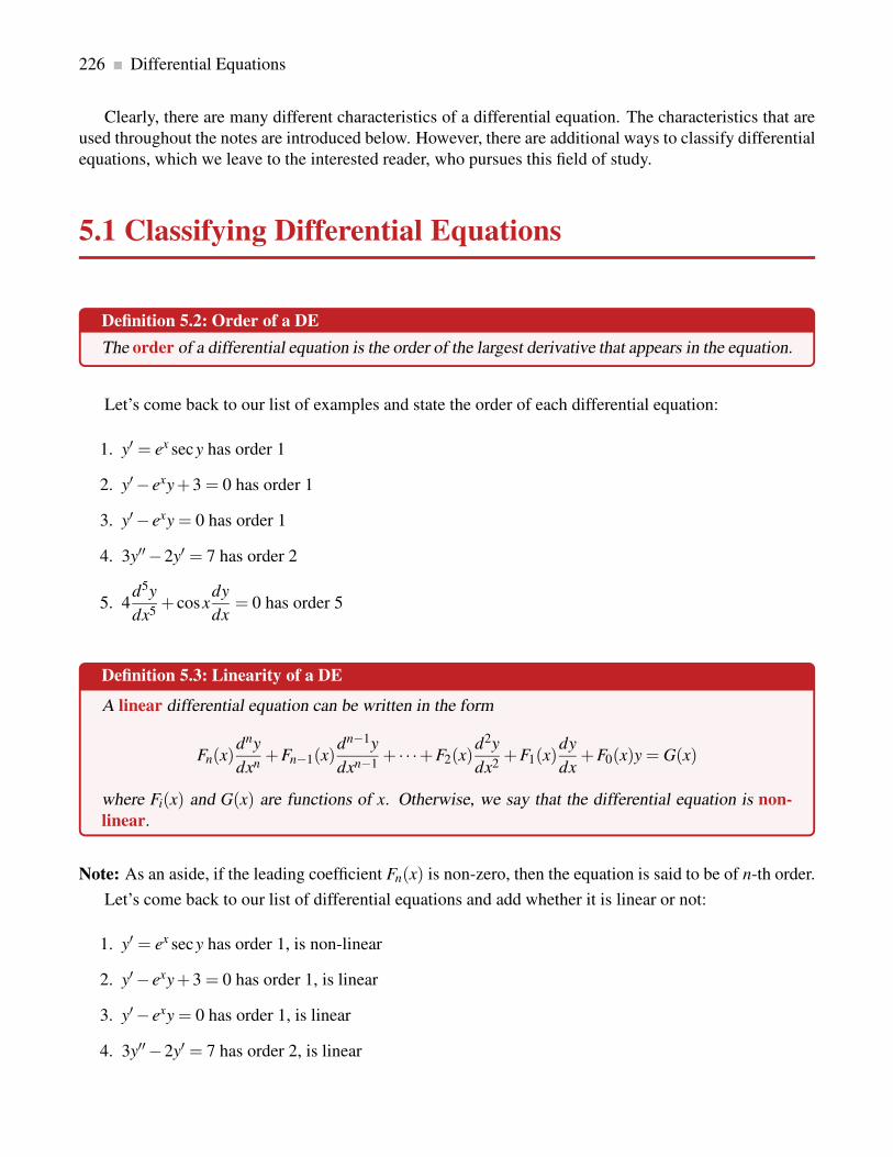
226 Differential Equations
Clearly, there are many different characteristics of a differential equation. The characteristics that are
used throughout the notes are introduced below. However, there are additional ways to classify differential
equations, which we leave to the interested reader, who pursues this field of study.
5.1 Classifying Differential Equations
Definition 5.2: Order of a DE
The order of a differential equation is the order of the largest derivative that appears in the equation.
Let’s come back to our list of examples and state the order of each differential equation:
1. y′ = ex secy has order 1
2. y′− exy+3 = 0 has order 1
3. y′− exy = 0 has order 1
4. 3y′′−2y′ = 7 has order 2
5. 4d5y
dx5+ cosx
dy
dx= 0 has order 5
Definition 5.3: Linearity of a DE
A linear differential equation can be written in the form
Fn(x)dny
dxn+Fn−1(x)
dn−1y
dxn−1+ · · ·+F2(x)
d2y
dx2+F1(x)
dy
dx+F0(x)y = G(x)
where Fi(x) and G(x) are functions of x. Otherwise, we say that the differential equation is non-
linear.
Note: As an aside, if the leading coefficient Fn(x) is non-zero, then the equation is said to be of n-th order.
Let’s come back to our list of differential equations and add whether it is linear or not:
1. y′ = ex secy has order 1, is non-linear
2. y′− exy+3 = 0 has order 1, is linear
3. y′− exy = 0 has order 1, is linear
4. 3y′′−2y′ = 7 has order 2, is linear
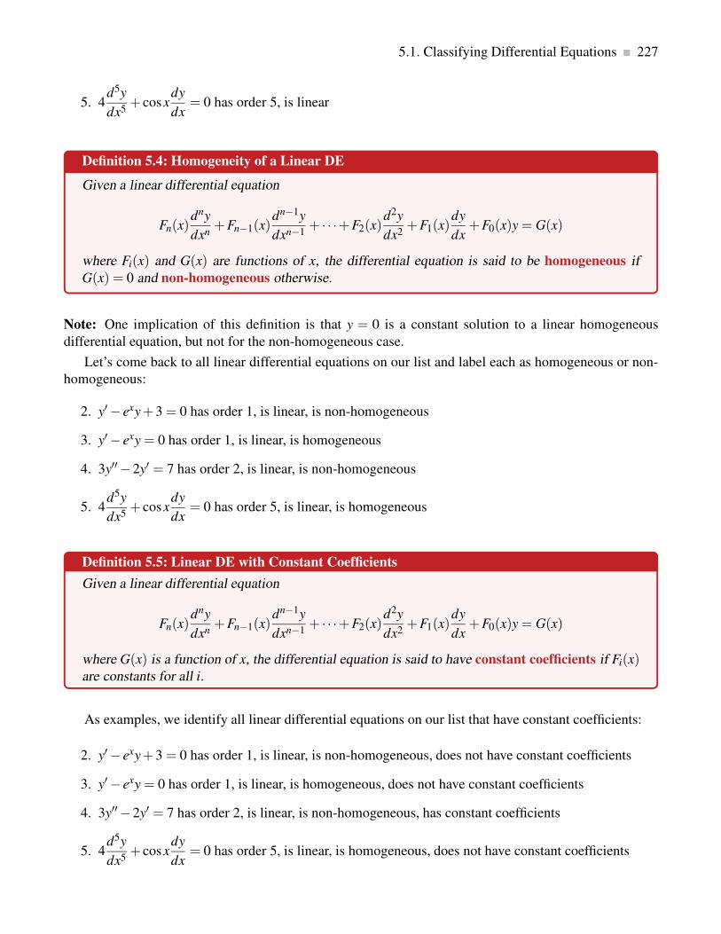
5.1. Classifying Differential Equations 227
5. 4d5y
dx5+ cosx
dy
dx= 0 has order 5, is linear
Definition 5.4: Homogeneity of a Linear DE
Given a linear differential equation
Fn(x)dny
dxn+Fn−1(x)
dn−1y
dxn−1+ · · ·+F2(x)
d2y
dx2+F1(x)
dy
dx+F0(x)y = G(x)
where Fi(x) and G(x) are functions of x, the differential equation is said to be homogeneous if
G(x) = 0 and non-homogeneous otherwise.
Note: One implication of this definition is that y = 0 is a constant solution to a linear homogeneous
differential equation, but not for the non-homogeneous case.
Let’s come back to all linear differential equations on our list and label each as homogeneous or non-
homogeneous:
2. y′− exy+3 = 0 has order 1, is linear, is non-homogeneous
3. y′− exy = 0 has order 1, is linear, is homogeneous
4. 3y′′−2y′ = 7 has order 2, is linear, is non-homogeneous
5. 4d5y
dx5+ cosx
dy
dx= 0 has order 5, is linear, is homogeneous
Definition 5.5: Linear DE with Constant Coefficients
Given a linear differential equation
Fn(x)dny
dxn+Fn−1(x)
dn−1y
dxn−1+ · · ·+F2(x)
d2y
dx2+F1(x)
dy
dx+F0(x)y = G(x)
where G(x) is a function of x, the differential equation is said to have constant coefficients if Fi(x)are constants for all i.
As examples, we identify all linear differential equations on our list that have constant coefficients:
2. y′− exy+3 = 0 has order 1, is linear, is non-homogeneous, does not have constant coefficients
3. y′− exy = 0 has order 1, is linear, is homogeneous, does not have constant coefficients
4. 3y′′−2y′ = 7 has order 2, is linear, is non-homogeneous, has constant coefficients
5. 4d5y
dx5+ cosx
dy
dx= 0 has order 5, is linear, is homogeneous, does not have constant coefficients

228 Differential Equations
Example 5.6: Newton’s Law of Cooling
The equation from Newton’s law of cooling,
dy
dt= k(M− y)
is a first order linear non-homogeneous differential equation with constant coefficients, where t is
time, k is the constant of proportionality, and M is the ambient temperature.
Exercises for Section 5.1
Exercise 5.1.1 Identify the order and linearity of each differential equation below.
(a) 5y′′′+3y′−4sin(y) = cos(x)
(b) 4d3y
dx3+2
dy
dx= exy
(c) ex dy
dx+ ex+y = e
(d) −d4y
dx4+ x
d3y
dx3− x2 d2y
dx2+ x3 dy
dx− x4y5 = 0
(e) f2(x)y′′+ f1(x)y
′+ f0(x)y−1 = 0, where fi(x) are non-constant functions of x
(f) tan(xy)y′ = sec(xy)
Exercise 5.1.2 Identify the homogeneity of each linear differential equation below.
(a) 5y′′′+3y′−4y = cos(x)
(b) 4d3y
dx3+2
dy
dx= exy
(c) ex dy
dx+ exy = e
(d) −d4y
dx4+ x
d3y
dx3− x2 d2y
dx2+ x3 dy
dx− x4y = 0
(e) f2(x)y′′+ f1(x)y
′+ f0(x)y−1 = 0, where fi(x) are non-constant functions of x
(f) tan(x)y′ = sec(x)y

5.2. First Order Differential Equations 229
Exercise 5.1.3 State whether the coefficients of each linear differential equation below are constant or
not.
(a) 5y′′′+3y′−4y = cos(x)
(b) 4d3y
dx3+2
dy
dx= exy
(c) ex dy
dx+ exy = e
(d) −d4y
dx4+ x
d3y
dx3− x2 d2y
dx2+ x3 dy
dx− x4y = 0
(e) f2(x)y′′+ f1(x)y
′+ f0(x)y−1 = 0, where fi(x) are non-constant functions of x
(f) tan(x)y′ = sec(x)y
5.2 First Order Differential Equations
In many fields such as physics, biology or business, a relationship is often known or assumed between
some unknown quantity and its rate of change, which does not involve any higher derivatives. It is therefore
of interest to study first order differential equations in particular.
Definition 5.7: First Order DE
A first order differential equation is an equation of the form F(t,y,y′) = 0. A solution of a first
order differential equation is a function f (t) that makes F(t, f (t), f ′(t)) = 0 for every value of t.
Here, F is a function of three variables which we label t, y, and y′. It is understood that y′ will
explicitly appear in the equation although t and y need not. The variable y itself is dependent on t, hence
it is understood that y′ must be the derivative of y with respect to t. Since only the first derivative of y
appears, but no higher order derivative, this is a first order differential equation.
Throughout the notes, we use the independent variable t as many applications are based on the inde-
pendent variable representing time. If no meaning is attributed to the independent variable, we may want
to write a first order differential equation in the usual manner as
F(x,y,y′) = 0.
Example 5.8: Simple First Order Differential Equation
y′ = t2+1 is a first order linear differential equation; F(t,y,y′) = y′− t2−1. Show that all solutions
to this equation are of the form y = t3/3+ t +C.

230 Differential Equations
Solution. We first note that y = t3/3+ t +C is a solution to the differential equation, since
d
dt
(
t3
3+ t +C
)
= t2+1,
for all C ∈ R.
We additionally need to show that there are no other solutions. To do so, we integrate the differential
equation:
y(t) =∫
(
t2 +1)
dt =t3
3+ t +C,
for some C ∈ R.
Thus, all solutions to the differential equation are of the form y = t3/3+ t +C. ♣
Example 5.9: Graphical Solution to First Order Differential Equation
Sketch various solutions to the differential equationdy
dx= 2x.
Solution. We integrate both sides of the differential equation to find
y =∫
2xdx = x2 +C
for any constant C ∈ R. This family of solutions are parabolas which are translated vertically, as shown in
the graph below taking C =−2,0,2.
−2
2
y = x2
y = x2 +2
y = x2 −2
x
y
♣
5.2.1. Initial Value Problems

5.2. First Order Differential Equations 231
Definition 5.10: Initial Conditions
Initial condition(s) are a set of points that the solution (or its derivatives) must satisfy.
Example 5.11: Initial Conditions
For a differential equation involving a function f (t), initial conditions are of the form:
f (t0) = f0, f ′(t0) = f1, f ′′(t0) = f2, . . .etc.
Definition 5.12: Initial Value Problem
An initial value problem (IVP) is a differential equation along with a set of initial conditions.
Example 5.13: First Order Initial Value Problem
Solve the initial value problem:dy
dx= 2x, y(0) = 2.
Solution. We had found in Example 5.9 that the solutions to the differential equation were the parabolas
y(x) = x2 +C.
So we use the initial condition to determine the constant C:
y(0) = (0)2+C = 2 =⇒ C = 2.
Therefore, the solution to the initial value problem is y = x2 +2, as shown in the graph below.
2
y = x2 +2
x
y

232 Differential Equations
♣
Example 5.14: Simple Initial Value Problem
Verify that the initial value problem y′ = t2+1, y(1) = 4 has solution f (t) = t3/3+ t +8/3.
Solution. Observe that f ′(t) = t2+1 and f (1) = 13/2+1+8/3 = 4 as required. ♣
The general first order equation is too general, so we can’t describe methods that will work on them
all, or even a large portion of them. We can make progress with specific kinds of first order differential
equations. For example, much can be said about equations of the form y′ = φ(t,y) where φ is a function
of the two variables t and y. Under reasonable conditions on φ , such an equation has a solution and the
corresponding initial value problem has a unique solution. However, in general, these equations can be
very difficult or impossible to solve explicitly.
Example 5.15: IVP for Newton’s Law of Cooling
Consider this specific example of an initial value problem for Newton’s law of cooling:
y′ = 2(25− y), y(0) = 40.
Discuss the solutions for this initial value problem.
Solution. We first note the zero of the equation: If y(t0) = 25, the right hand side of the differential
equation is zero, and so the constant function y(t) = 25 is a solution to the differential equation. It is
not a solution to the initial value problem, since y(0) 6= 25. (The physical interpretation of this constant
solution is that if a liquid is at the same temperature as its surroundings, then the liquid will stay at that
temperature.) So long as y is not 25, we can rewrite the differential equation as
dy
dt
1
25− y= 2
1
25− ydy = 2dt,
so∫
1
25− ydy =
∫
2dt,
that is, the two antiderivatives must be the same except for a constant difference. We can calculate these
antiderivatives and rearrange the results:
∫
1
25− ydy =
∫
2dt
(−1) ln |25− y| = 2t +C0
ln |25− y| = −2t −C0 =−2t +C
|25− y| = e−2t+C = e−2teC
y−25 = ±eCe−2t
y = 25± eCe−2t = 25+Ae−2t .

5.2. First Order Differential Equations 233
Here A =±eC =±e−C0 is some non-zero constant. Since we want y(0) = 40, we substitute and solve for
A:
40 = 25+Ae0 =⇒ A = 15.
Therefore, y = 25+ 15e−2t is a solution to the initial value problem. Note that y is never 25, so this
makes sense for all values of t. However, if we allow A = 0 we get the solution y = 25 to the differential
equation, which would be the solution to the initial value problem if we were to require y(0) = 25. Thus,
y = 25+Ae−2t describes all solutions to the differential equation y′ = 2(25− y), and all solutions to the
associated initial value problems. ♣
5.2.2. Separable Equations
Why could we solve Example 5.15 from the previous section? Our solution depended on rewriting the
equation so that all instances of y were on one side of the equation and all instances of t were on the
other. Of course, in this case the only t was originally hidden, since we didn’t write dy/dt in the original
equation. This is not required, however. This idea of being able to separate the independent and dependent
variables in a first order differential equation leads to a classification of first order differential equations
into separable and non-separable equations as follows.
Definition 5.16: Separable DE
A first order differential equation is separable if it can be written in the form
dy
dt= f (t)g(y).
Let’s come back to all first order differential equations on our list from the previous section and decide
which ones are separable or not:
1. y′ = ex secy has order 1, is non-linear, is separable
2. y′− exy+3 = 0 has order 1, is linear, is not separable
3. y′− exy = 0 has order 1, is linear, is separable
As in the examples, we can attempt to solve a separable equation by converting to the form
∫
1
g(y)dy =
∫
f (t)dt.
This technique is called separation of variables. The simplest (in principle) sort of separable equation is
one in which g(y) = 1, in which case we attempt to solve
∫
1dy =∫
f (t)dt.
We can do this if we can find an antiderivative of f (t).

234 Differential Equations
As we have seen so far, a differential equation typically has an infinite number of solutions. Such
a solution is called a general solution. A corresponding initial value problem will give rise to just one
solution. Such a solution in which there are no unknown constants remaining is called a particular
solution.
The general approach to separable equations is as follows: Suppose we wish to solve y′ = f (t)g(y)where f and g are continuous functions. If g(a) = 0 for some a then y(t) = a is a constant solution of the
equation, since in this case y′ = 0 = f (t)g(a). For example, y′ = y2−1 has constant solutions y(t) = 1 and
y(t) =−1.
To find the non-constant solutions, we note that the function 1/g(y) is continuous where g 6= 0, so 1/g
has an antiderivative G. Let F be an antiderivative of f . Now we write
G(y) =
∫
1
g(y)dy =
∫
f (t)dt = F(t)+C,
so G(y) = F(t)+C. Now we solve this equation for y.
Of course, there are a few places this ideal description could go wrong: Finding the antiderivatives
G and F , and solving the final equation for y. The upshot is that the solutions to the original differential
equation are the constant solutions, if any, and all functions y that satisfy G(y) = F(t)+C.
Guideline for Separation of Variables
Given the differential equationdy
dt= f (t)g(y),
follow these steps to find the non-constant solutions.
1. Separate the variables:dy
g(y)= f (t)dt
2. Apply the integration operator:∫
dy
g(y)=∫
f (t)dt
3. If an antiderivative exists for f and for 1/g, and we can solve for y, then
G(y) = F(t)+C
for some constant C.
Example 5.17: Solving a Separable Differential Equation
Solve the differential equation y′ = 2t(25− y).
Solution. This is almost identical to the previous example. As before, y(t) = 25 is a solution. If y 6= 25,
∫
1
25− ydy =
∫
2t dt

5.2. First Order Differential Equations 235
(−1) ln |25− y| = t2+C0
ln |25− y| = −t2−C0 =−t2 +C
|25− y| = e−t2+C = e−t2eC
y−25 = ±eCe−t2
y = 25± eCe−t2= 25+Ae−t2
.
As before, all solutions are represented by y = 25+Ae−t2, allowing A to be zero. ♣
Example 5.18: Solving a Seperable Differential Equation
Find the solutions to the differential equation
sec(t)dy
dt− ey+sin(t) = 0.
Solution. We begin by separating the variables and get
sec(t)dy
dt= ey+sin(t)
sec(t)dy
dt= eyesin(t)
e−y dy =esin(t)
sec(t)dt = cos(t)esin(t) dt
Now integrate both sides to obtain
∫
e−y dy =
∫
cos(t)esin(t) dt
−e−y = esin(t)+C
y =− ln(
D− esin(t))
For convenience, we left out the absolute value in the argument of the logarithm. As in the previous
examples, care must be taken to ensure that the argument of the logarithm is positive for a given value of
D.
Therefore, the solutions to the differential equation are given by
y =− ln(
D− esin(t))
,
for some constant D. ♣
5.2.3. Simple Growth and Decay Model

236 Differential Equations
Example 5.19: Rate of Change Proportional to Size
Find the solutions to the differential equation y′ = ky, which models a quantity y that grows or
decays proportionally to its size depending on whether k is positive or negative.
Solution. The constant solution is y(t) = 0; of course this will not be the solution to any interesting initial
value problem. For the non-constant solutions, we proceed much as before:
∫
1
ydy =
∫
k dt
ln |y| = kt +C
|y| = ekteC
y = ±eCekt
y = Aekt .
Again, if we allow A = 0 this includes the constant solution, and we can simply say that y = Aekt is the
general solution. With an initial value we can easily solve for A to get the solution of the initial value
problem. In particular, if the initial value is given for time t = 0, y(0) = y0, then A = y0 and the solution is
y = y0ekt . ♣
The constant k in the above differential equation is referred to as the growth rate constant. Further-
more, this type of differential equation is known as a simple model for growth and decay of some quantity,
since it only considers that the growth rate is proportional to the size of the quantity itself without any
other factors influencing y. The graph below shows the typical J-shape of such a solution for some y0.
y0
growth rate of y
accelerates
t
y

5.2. First Order Differential Equations 237
Simple Growth and Decay Model
The differential equationdy
dt= ky
with growth rate constant k models simple growth and decay of a quantity y at time t with solution
y = y0ekt ,
where y0 is the initial value at time t = 0.
When k > 0, this describes certain simple cases of population growth: It says that the change in the
population y is proportional to the population. The underlying assumption is that each organism
in the current population reproduces at a fixed rate, so the larger the population the more new
organisms are produced. While this is too simple to model most real populations, it is useful in
some cases over a limited time.
When k < 0, the differential equation describes a quantity that decreases in proportion to the current
value. This can be used to model radioactive decay.
Note: The simple growth and decay model is unrestricted because the quantity y grows without bound as
t → ∞ if k > 0. In the decay case, the solution only becomes unbounded if time t is allowed to approach
−∞.
Example 5.20: Simple Growth Model
Suppose $5,000 is deposited into an account which earns continuously compounded interest. Under
these conditions, the balance in the account grows at a rate proportional to the current balance.
Suppose that after 4 years, the account is worth $7,000.
(a) How much is the account worth after 5 years?
(b) How many years does it take for the balance to double?
Solution. Let y(t) denote the balance in the account at the start of year t. Then
dy
dt= ky(t),
for some constant k. We can solve this differential equation using separation of variables to obtain
y(t) = y0ekt = 5000ekt ,
where we used the fact that y(0) = 5,000. We know that y(4) = 7000, which we now use to solve for k:
7000 = 5000e4k
e4k =7
5
k =ln(
75
)
4

238 Differential Equations
Therefore,
y(t) = 5000eln(7/5)
4 t .
(a) After 5 years, the balance in the account is
y(5) = 5000eln(7/5)
4 ·5 ≈ $7614.30.
(b) We wish to find t so that y(t) = 10000.
10000 = 5000eln(7/5)
4 t
eln(7/5)
4 t = 2
t =ln(16)
ln(
75
) ≈ 8.24
Thus, it takes just over 8 years for the balance in the account to double in value.
♣
5.2.4. Logistic Growth Model
The simple growth model is unrealistic because a quantity that represents something from real life, say,
population, does not grow unrestricted. Typically, food resources, competition, predators, or diseases, to
name but a few factors, influence the growth of the population, and how much of the population can be
sustained in such an environment.
A more realistic model is the so-called logistic growth model, which mimics that as a quantity is
growing other factors will influence the growth and slow it down until a certain maximum size is being
approached. For example, if a population is growing, then food may become scarce or diseases may break
out among the population, and the population growth slows down until a certain sustainable size is reached.
Replacing k in the simple model with r(M − y) achieves that as the quantity y increases the growth rate
decreases, and furthermore, that the maximum population size that is sustained is M. This maximum is
referred to as the carrying capacity. So the simple model becomes
dy
dt= ry(M− y)
for some positive r and M.
In other words, the rate of growth of the quantity y is proportional to both itself and the remaining
carrying capacity that the quantity can still grow to. As usual, r is the growth rate constant.
To solve this first order non-linear differential equation, notice that the equation is separable
dy
y(M− y)= r dt.

5.2. First Order Differential Equations 239
Integrating both sides we obtain∫
dy
y(M− y)=
∫
r dt
∫
(
1
y+
1
M− y
)
dy =∫
rM dt
ln |y|− ln |M− y|= rMt +C
ln
∣
∣
∣
∣
M− y
y
∣
∣
∣
∣
=−rMt −C
∣
∣
∣
∣
M− y
y
∣
∣
∣
∣
= e−rMt−C
M− y
y= Ae−rMt ,
where A =M− y0
y0for t0 = 0.
Lastly, we solve for y and get the solution
y =M
1+Ae−rMtwith A =
M− y0
y0
for some constant y0 at time t0 = 0.
The graph below shows the typical S-shape of such a solution for some y0 between 0 and M. For
y0 > M, the solution decays exponentially to M. And for y0 = M, the solution remains constant.
y0 =M
1+A
M
point of max
growth
growth rate
decreasing
growth rate
increasing
t
y
Note: Let us rewritedy
dt= ry(M− y)
asdy
dt= rM
(
M− y
M
)
y.
Then we can make the following interpretations.

240 Differential Equations
1. When the quantity y is small, then the termM− y
Mis close in value to one, and so the differential
equationdy
dt= ry(M− y) ≈ rMy.
In other words, the growth is exponential.
2. However, when the quantity y is near that of the carrying capacity M, then the termM− y
Mis close
in value to zero. Hence, the less carrying capacity that remains the more the growth rate is slowed
down.
Logistic Growth Model
The differential equationdy
dt= ry(M− y)
with positive growth constant r and carrying capacity M models logistic growth of a quantity y at
time t with solution
y =M
1+Ae−rMt,
where A =M− yo
y0at time t0 = 0.
Exercises for Section 5.2
Exercise 5.2.1 Which of the following equations are separable?
(a) y′ = sin(ty)
(b) y′ = etey
(c) yy′ = t
(d) y′ = (t3− t)arcsin(y)
(e) y′ = t2 lny+4t3 lny
Exercise 5.2.2 Identify the constant solutions (if any) of the following differential equations.
(a) y′ = t siny (b) y′ = tey
Exercise 5.2.3 Solve the following differential equations. You may leave your solution in implicit form:
that is, you may stop once you have done the integration, without solving for y.

5.2. First Order Differential Equations 241
(a) y′ = 1/(1+ t2)
(b) y′ = ln t
(c) y′ = t/y
(d) y′ = y2 −1
(e) y′ = t/(y3−5)
(f) y′ = k(M− f (t))
Exercise 5.2.4 Solve the following initial value problems.
(a) y′ = tn, y(0) = 1 and n ≥ 0
(b) y′ = y1/3, y(0) = 0
(c) y′ = ky, y(0) = 2, and y′(0) = 3
Exercise 5.2.5 After 10 minutes in Jean-Luc’s room, his tea has cooled to 40◦ Celsius from 100◦ Celsius.
The room temperature is 25◦ Celsius. How much longer will it take to cool to 35◦?
Exercise 5.2.6 A radioactive substance obeys the equation y′ = ky where k < 0 and y is the mass of the
substance at time t. Suppose that initially, the mass of the substance is y(0) = M > 0. At what time does
half of the mass remain? (This is known as the half life. Note that the half life depends on k but not on
M.)
Exercise 5.2.7 Bismuth-210 has a half life of five days. If there is initially 600 milligrams, how much is
left after 6 days? When will there be only 2 milligrams left?
Exercise 5.2.8 The half life of carbon-14 is 5730 years. If one starts with 100 milligrams of carbon-14,
how much is left after 6000 years? How long do we have to wait before there is less than 2 milligrams?
Exercise 5.2.9 A certain species of bacteria doubles its population (or its mass) every hour in the lab.
The differential equation that models this phenomenon is y′ = ky, where k > 0 and y is the population of
bacteria at time t. What is y?
Exercise 5.2.10 If a certain microbe doubles its population every 4 hours and after 5 hours the total
population has mass 500 grams, what was the initial mass?
Exercise 5.2.11 Given the logistic equation y′ = ky(M− y),
(a) Solve the differential equation for y in terms of t.
(b) Sketch the graph of the solution to this equation when M = 1000, k = 0.002, y(0) = 1.
Exercise 5.2.12 The biologist G. F. Gause studied the growth of the protozoan Paramecium in the early
1930s. Through his data, he figured out that the relative growth rate is 0.7944 when y(0) = 2, and the
carrying capacity is 64. This leads to the logistic model
dy
dt= 0.7944
(
1− y
64
)
, y(0) = 2,
where time is measured in days.

242 Differential Equations
(a) Solve the differential equation for y in terms of t.
(b) How long will it take for the protozoa to reach 30?
(c) Sketch the graph of the solution to this equation.
5.3 First Order Linear Differential Equations
5.3.1. Homogeneous DEs
A simple, but important and useful, type of separable equation is the first order homogeneous linear
equation:
Definition 5.21: First Order Homogeneous Linear DE
A first order homogeneous linear differential equation is one of the form y′ + p(t)y = 0 or
equivalently y′ =−p(t)y.
We have already seen a first order homogeneous linear differential equation, namely the simple growth
and decay model y′ = ky.
Since first order homogeneous linear equations are separable, we can solve them in the usual way:
y′ = −p(t)y∫
1
ydy =
∫
−p(t)dt
ln |y| = P(t)+C
y = ±eP(t)
y = AeP(t),
where P(t) is an antiderivative of −p(t). As in previous examples, if we allow A = 0 we get the constant
solution y = 0.
Example 5.22: Solving an IVP
Solve the initial value problem
y′+ ycos t = 0,
subject to
(a) y(0) = 1/2 (b) y(2) = 1/2
Solution. We start with
P(t) =∫
−cos t dt =−sin t,

5.3. First Order Linear Differential Equations 243
so the general solution to the differential equation is
y = Ae−sin t .
(a) To compute the constant coefficient A, we substitute:
1
2= Ae−sin0 = A,
so the solutions is
y =1
2e−sin t .
(b) To compute the constant coefficient A, we substitute:
1
2= Ae−sin2
A =1
2esin2
so the solution is
y =1
2esin2e−sin t .
♣
Example 5.23: Solving an IVP
Solve the initial value problem ty′+3y = 0, y(1) = 2, assuming t > 0.
Solution. We write the equation in standard form: y′+3y/t = 0. Then
P(t) =
∫
−3
tdt =−3ln t
and
y = Ae−3ln t = At−3.
Substituting to find A: 2 = A(1)−3 = A, so the solution is y = 2t−3. ♣
5.3.2. Non-Homogeneous DEs
As you might guess, a first order non-homogeneous linear differential equation has the form y′ +p(t)y = f (t). Not only is this closely related in form to the first order homogeneous linear equation, we
can use what we know about solving homogeneous equations to solve the general linear equation.
Definition 5.24: First Order Non-Homogeneous Linear DE
A first order non-homogeneous linear differential equation is one of the form
y′+ p(t)y = f (t).

244 Differential Equations
Note: When the coefficient of the first derivative is one in the first order non-homogeneous linear differ-
ential equation as in the above definition, then we say the DE is in standard form.
Let us now discuss how we can find all solutions to a first order non-homogeneous linear differential
equation. Suppose that y1(t) and y2(t) are solutions to y′+ p(t)y = f (t). Let g(t) = y1 − y2. Then
g′(t)+ p(t)g(t) = y′1 − y′2 + p(t)(y1− y2)= (y′1 + p(t)y1)− (y′2 + p(t)y2)= f (t)− f (t) = 0.
In other words, g(t) = y1 − y2 is a solution to the homogeneous equation y′ + p(t)y = 0. Turning this
around, any solution to the linear equation y′+ p(t)y = f (t), call it y1, can be written as y2 + g(t), for
some particular y2 and some solution g(t) of the homogeneous equation y′+ p(t)y = 0. Since we already
know how to find all solutions of the homogeneous equation, finding just one solution to the equation
y′+ p(t)y = f (t) will give us all of them.
Theorem 5.25: General Solution of First Order Non-Homogeneous Linear DE
Given a first order non-homogeneous linear differential equation
y′− p(t)y = f (t),
let h(t) be a particular solution, and let g(t) be the general solution to the corresponding homoge-
neous DE
y′− p(t)y = 0.
Then the general solution to the non-homogeneous DE is constructed as the sum of the above two
solutions:
y(t) = g(t)+h(t).
Variation of Parameters
We now introduce the first one of two methods discussed in these notes to solve a first order non-
homogeneous linear differential equation. Again, it turns out that what we already know helps. We know
that the general solution to the homogeneous equation y′+ p(t)y= 0 looks like AeP(t), where P(t) is an an-
tiderivative of −p(t). We now make an inspired guess: Consider the function v(t)eP(t), in which we have
replaced the constant parameter A with the function v(t). This technique is called variation of parame-
ters. For convenience write this as s(t) = v(t)h(t), where h(t) = eP(t) is a solution to the homogeneous
equation. Now let’s compute a bit with s(t):
s′(t)+ p(t)s(t) = v(t)h′(t)+ v′(t)h(t)+ p(t)v(t)h(t)= v(t)(h′(t)+ p(t)h(t))+ v′(t)h(t)= v′(t)h(t).
The last equality is true because h′(t)+ p(t)h(t)= 0, since h(t) is a solution to the homogeneous equation.
We are hoping to find a function s(t) so that s′(t)+ p(t)s(t) = f (t); we will have such a function if we

5.3. First Order Linear Differential Equations 245
can arrange to have v′(t)h(t) = f (t), that is, v′(t) = f (t)/h(t). But this is as easy (or hard) as finding an
antiderivative of f (t)/h(t). Putting this all together, the general solution to y′+ p(t)y = f (t) is
v(t)h(t)+AeP(t) = v(t)eP(t)+AeP(t).
Method of Variation of Parameters
Given a first order non-homogeneous linear differential equation
y′+ p(t)y = f (t),
using variation of parameters the general solution is given by
y(t) = v(t)eP(t)+AeP(t),
where v′(t) = eP(t) f (t) and P(t) is an antiderivative of −p(t).
Note: The method of variation of parameters makes more sense after taking linear algebra since the
method uses determinants. We therefore restrict ourselves to just one example to illustrate this method.
Example 5.26: Solving an IVP Using Variation of Parameters
Find the solution of the initial value problem y′+3y/t = t2, y(1) = 1/2.
Solution. First we find the general solution; since we are interested in a solution with a given condition at
t = 1, we may assume t > 0. We start by solving the homogeneous equation as usual; call the solution g:
g = Ae−∫
(3/t)dt = Ae−3ln t = At−3.
Then as in the discussion, h(t) = t−3 and v′(t) = t2/t−3 = t5, so v(t) = t6/6. We know that every solution
to the equation looks like
v(t)t−3+At−3 =t6
6t−3+At−3 =
t3
6+At−3.
Finally we substitute to find A:
1
2=
(1)3
6+A(1)−3 =
1
6+A
A =1
2− 1
6=
1
3.
The solution is then
y =t3
6+
1
3t−3.
♣

246 Differential Equations
Integrating Factor
Another common method for solving such a differential equation is by means of an integrating factor.
In the differential equation y′+ p(t)y = f (t), we note that if we multiply through by a function I(t) to get
I(t)y′+ I(t)p(t)y= I(t) f (t), the left hand side looks like it could be a derivative computed by the Product
Rule:d
dt(I(t)y) = I(t)y′+ I′(t)y.
Now if we could choose I(t) so that I′(t) = I(t)p(t), this would be exactly the left hand side of the
differential equation. But this is just a first order homogeneous linear equation, and we know a solution
is I(t) = eQ(t), where Q(t) =∫
p(t)dt. Note that Q(t) = −P(t), where P(t) appears in the variation of
parameters method and P′(t) =−p(t). Now the modified differential equation is
e−P(t)y′+ e−P(t)p(t)y = e−P(t) f (t)d
dt(e−P(t)y) = e−P(t) f (t).
Integrating both sides gives
e−P(t)y =
∫
e−P(t) f (t)dt
y = eP(t)∫
e−P(t) f (t)dt.
Note: If you look carefully, you will see that this is exactly the same solution we found by variation
of parameters, because e−P(t) f (t) = f (t)/h(t). Some people find it easier to remember how to use the
integrating factor method, rather than variation of parameters. Since ultimately they require the same
calculation, you should use whichever of the two methods appeals to you more.
Definition 5.27: Integrating Factor
Given a first order non-homogeneous linear differential equation
y′+ p(t)y = f (t),
the integrating factor is given by
I(t) = e∫
p(t)dt .

5.3. First Order Linear Differential Equations 247
Method of Integrating Factor
Given a first order non-homogeneous linear differential equation
y′+ p(t)y = f (t),
follow these steps to determine the general solution y(t) using an integrating factor:
1. Calculate the integrating factor I(t).
2. Multiply the standard form equation by I(t).
3. Simplifly the left-hand side tod
dt[I(t)y] .
4. Integrate both sides of the equation.
5. Solve for y(t).
The solution can be compactly written as
y(t) = e−∫
p(t)dt
[
∫
e∫
p(t)dt f (t)dt+C
]
.
Using this method, the solution of the previous example would look just a bit different.
Example 5.28: Solving an IVP Using Integrating Factor
Find the solution of the initial value problem y′+3y/t = t2, y(1) = 1/2.
Solution. Notice that the differential equation is already in standard form. We begin by computing the
integrating factor and obtain
I(t) = e∫ 3
t dt = e3ln t = t3
for t > 0.
Next, we multiply both sides of the DE with I(t) and get
t3
[
y′+3
yy
]
= t3t2
y3y′+3t2y = t5
which simplifies tod
dt
[
t3y]
= t5.

248 Differential Equations
Now we integrate both sides with respect to t and solve for y:∫
d
dt
[
t3y]
dt =
∫
t5 dt
t3y =t6
6+C
y =t3
6+
C
t3.
Lastly, we use the initial value y(1) = 1/2 to find C:
y(1) =13
6+
C
13=
1
2=⇒ C =
1
3.
Hence, the solution to the DE is
y =t3
6+
1
3t2.
♣
Example 5.29: General Solution Using Integrating Factor
Determine the general solution of the differential equation
dy
dt+3t2y = 6t2.
Solution. We see that the differential equation is in standard form. We then compute the integrating factor
as
I(t) = e∫
3t2 dt = et3,
where we took the arbitrary constant of integration to be zero.
Therefore, we can write the DE as
et3 [
y′+3t2y]
= 6t2et3
d
dt
[
et3y]
= 6t2et3.
Integrating both sides with respect to t gives
et3y = 6
∫
t2et3dt
We solve this integral by making the substitution u = t3, du = 3t2 dt:∫
t2et3dt =
1
3
∫
eu du =1
3eu +C =
1
3et3
+C.
Thus,
et3y = 2et3
+C
y = 2+Ce−t3
.

5.3. First Order Linear Differential Equations 249
The general solution to the DE is therefore
y = 2+Ce−t3,
for C ∈ R. ♣
Exercises for Section 5.3
Exercise 5.3.1 Find the general solution of the following homogeneous differential equations.
(a) y′+5y = 0
(b) y′−2y = 0
(c) y′+y
1+ t2= 0
(d) y′+ t2y = 0
Exercise 5.3.2 Solve the following initial value problems concerning homogeneous DEs.
(a) y′+ y = 0, y(0) = 4
(b) y′−3y = 0, y(1) =−2
(c) y′+ ysin t = 0, y(π) = 1
(d) y′+ yet = 0, y(0) = e
(e) y′+ y√
1+ t4 = 0, y(0) = 0
(f) y′+ ycos(et) = 0, y(0) = 0
(g) ty′−2y = 0, y(1) = 4
(h) t2y′+ y = 0, y(1) =−2, t > 0
(i) t3y′ = 2y, y(1) = 1, t > 0
(j) t3y′ = 2y, y(1) = 0, t > 0
Exercise 5.3.3 Find the general solution of the following non-homogeneous differential equations.
(a) y′+4y = 8
(b) y′−2y = 6
(c) y′+ ty = 5t
(d) y′+ ety =−2et
(e) y′− y = t2
(f) 2y′+ y = t
Exercise 5.3.4 Find the general solution of the following non-homogeneous differential equations on the
restricted domain.
(a) ty′−2y = 1/t, t > 0
(b) ty′+ y =√
t, t > 0
(c) y′ cos t + ysint = 1, −π/2 < t < π/2
(d) y′+ ysec t = tan t, −π/2 < t < π/2
Exercise 5.3.5 Solve the following initial value problems concerning non-homogeneous DEs.

250 Differential Equations
(a) y′+4y = 8,y(0) = 1
(b) y′−2y = 6,y(0) = 3
(c) y′+ ty = 5t,y(2) = 1
(d) y′+ ety =−2et ,y(0) = e−1
(e) y′− y = t2,y(0) = 4
(f) 2y′+ y = t,y(1) =−1
Exercise 5.3.6 A function y(t) is a solution of y′+ ky = 0. Suppose that y(0) = 100 and y(2) = 4. Find k
and find y(t).
Exercise 5.3.7 A function y(t) is a solution of y′+ tky = 0. Suppose that y(0) = 1 and y(1) = e−13. Find
k and find y(t).
Exercise 5.3.8 A bacterial culture grows at a rate proportional to its population. If the population is one
million at t = 0 and 1.5 million at t = 1 hour, find the population as a function of time.
Exercise 5.3.9 A radioactive element decays with a half-life of 6 years. If a mass of the element weighs
ten pounds at t = 0, find the amount of the element at time t.
5.4 Approximation
We have seen how to solve a restricted collection of differential equations, or more accurately, how to
attempt to solve them—we still may not be able to find the required antiderivatives. Not surprisingly,
non-linear equations can be even more difficult to solve. Yet much is known about solutions to some more
general equations.
Suppose φ(t,y) is a function of two variables. A more general class of first order differential equations
has the form y′ = φ(t,y). This is not necessarily a linear first order equation, since φ may depend on y
in some complicated way; note however that y′ appears in a very simple form. Under suitable conditions
on the function φ , it can be shown that every such differential equation has a solution, and moreover
that for each initial condition the associated initial value problem has exactly one solution. In practical
applications this is obviously a very desirable property.
5.4.1. Slope Field
There are many ways to visualize solutions of differential equations of the form y′ = φ(t,y). A particularly
simple and useful way to do so is using a so-called slope field, where we make use of the fact that φ(t,y)is just the slope of the solution at any point (t,y). This allows us to generate a plot in the t-y-plane of the
slope at any point as shown below for the DE
dy
dy=− ty
1+ t2.
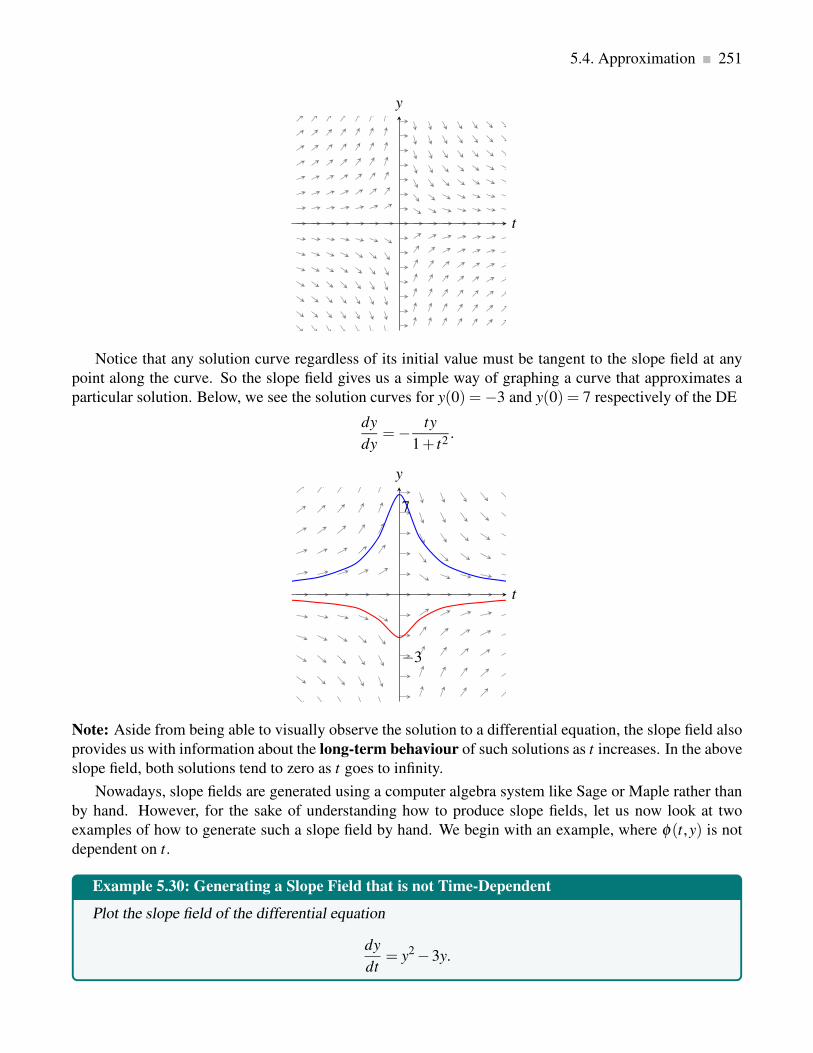
5.4. Approximation 251
t
y
Notice that any solution curve regardless of its initial value must be tangent to the slope field at any
point along the curve. So the slope field gives us a simple way of graphing a curve that approximates a
particular solution. Below, we see the solution curves for y(0) =−3 and y(0) = 7 respectively of the DE
dy
dy=− ty
1+ t2.
−3
7
t
y
Note: Aside from being able to visually observe the solution to a differential equation, the slope field also
provides us with information about the long-term behaviour of such solutions as t increases. In the above
slope field, both solutions tend to zero as t goes to infinity.
Nowadays, slope fields are generated using a computer algebra system like Sage or Maple rather than
by hand. However, for the sake of understanding how to produce slope fields, let us now look at two
examples of how to generate such a slope field by hand. We begin with an example, where φ(t,y) is not
dependent on t.
Example 5.30: Generating a Slope Field that is not Time-Dependent
Plot the slope field of the differential equation
dy
dt= y2 −3y.

252 Differential Equations
Solution. Notice that the right side of the DE is not dependent on t. This means that if we plot the slopes
along a vertical line of the t-y-plane, we can produce the full slope field by simply copying these slopes to
the left and right as t decreases and increases.
We begin by computing the slopes for y ranging between -5 and 5 in step-sizes of one:
y −5 −4 −3 −2 −1 0 1 2 3 4 5
y′ 40 28 18 10 5 0 −2 −2 0 4 1
Next, we graph short tangent line segments at the points (t,y) for, say, t = 2:
t = 2−5
−4
−3
−2
−1
1
2
3
4
5
t
y
Lastly, we produce the full slope field by making copies of this vertical slice of slopes to the left and
right as shown below for values of t between -5 and 5:
−5
5
t
y
♣
Let us now look at an example, where φ(t,y) depends on t and y, in which case the computations are
more labourious.

5.4. Approximation 253
Example 5.31: Generating a Slope Field that is Time-Dependent
Plot the slope field of the differential equation
dy
dt= t − y2.
Solution. Notice that the right side of the differential equation is dependent on both t and y. We can
therefore not replicate slopes as showcased in the above example, but must employ a different method.
In fact, we demonstrate two methods, one that is crude but will always work, and one where we identify
places where the derivative will be constant.
Method 1: In this approach, we simply compute the slope values at integer coordinates for a certain
section of the t-y-plane, say the [−5,5]× [−5,5] grid shown below.
t
y
Before we start computing slope values, we investigate the right side of the differential equation and
take note of any symmetry that might reduce the amount of computations that we need to do. Here, we
notice the symmetry in y, that is, the slope for a certain y-value is the same as for the corresponding
negative y-value at the same value of t. This reduces our computations by half. Let’s begin calculating the
slope values for −5 ≤ y ≤ 5 when t = 5:
y −5 −4 −3 −2 −1 0 1 2 3 4 5
y′ −20 −11 −4 1 4 5 4 1 −4 −11 −20
Next, we draw short tangent line segments at the grid points (5,y) as before to get the graph as shown:

254 Differential Equations
−5
5
t
y
We repeat the computations for all integer values of t and y on the [−5,5]× [−5,5] grid to obtain the
slope field below.
−5
5
t
y
Method 2: In this approach, we look for places where the derivative will be constant, that is, where
t − y2 = k,
for some constant k. When k = 0, then this produces the curve y2 = t, which is the parabola shown below:

5.4. Approximation 255
k = 0
t
y
At all points along this curve, the slope of the differential equation must be zero (see below).
k = 0
t
y
In fact, all curves y2 = t − k are parabolas shifted to the left or right depending on the value of k, and
the slopes along any of these curves must have the value k, which is shown in the following graph.
k = 0k = 2k = 4
k =−2k =−4
t
y
Ignoring the parabolas on the above plot, we have generated the desired slope field. ♣
Note:

256 Differential Equations
1. The curves produced by the equation φ(t,y) = k for k constant and any DE y′ = φ(t,y), as in the
above example with t − y2 = k, are referred to as a family of curves. They arise with differential
equations but also other areas of mathematics.
2. Method 1 in Example 5.31 does not depend on an integer grid. One can choose any points to
compute the slopes.
We now provide one example that outlines how to draw the solution curve to a differential equation
on a slope field for a particular initial value. We point out that in this process, we often make use of the
simplest slope, namely the zero slope, as it eases computations.
Example 5.32: Graphing Solution Curves on a Slope Field
Given the slope field from Example 5.31 for the differential equation
dy
dt= t − y2,
graph the solution curves for the following initial values:
(a) y(0) =−2 (b) y(0) = 0 (c) y(0) = 2
Solution.
(a) We start by indicating the point y(0) = −2 and then follow the solution trajectory forward and
backward in the independent variable t based on the little tangent lines. The solution curve is shown
below to the left.
(b) and (c) A similar approach as in part (a) produces the solution curves when y(0) = 0 shown below
centre and when y(0) = 2 shown below to the right.
−2
t
y
(a)
t
y
(b)
2
t
y
(c)
♣

5.4. Approximation 257
Even when a differential equation can be solved explicitly, the slope field can help in understanding
what the solutions look like with various initial conditions. Recall the logistic equation y′ = ky(M − y):y is a population at time t, M is a measure of how large a population the environment can support, and k
measures the reproduction rate of the population. Figure 5.1 shows a slope field for this equation that is
quite informative. It is apparent that if the initial population is smaller than M it rises to M over the long
term, while if the initial population is greater than M it decreases to M.
Figure 5.1: A slope field for y′ = 0.2y(10− y).
5.4.2. Euler’s Method
Not all differential equations that are important in practice can be solved exactly, so techniques have been
developed to numerically approximate solutions. Such techniques are referred to as numerical methods,
which are often quite accurate, and typically executed by means of a computer and so also fast. When exact
computation are not possible or excessively complicated, then numerical methods are chosen. We describe
one such method, Euler’s Method, which is simple though not particularly useful compared to some more
sophisticated techniques. Euler’s method is based on the method of linearization by approximating the
solution curve with a succession of linearizations over an interval as shown in the figure below.
exact solution
(t0,y0)
error
approximation
t
y

258 Differential Equations
Suppose we wish to approximate a solution to the initial value problem y′ = φ(t,y), y(t0) = y0, for
t ≥ t0. Under reasonable conditions on φ , we know the solution exists, represented by a curve in the t-y-
plane; call this solution f (t) as shown below. The point (t0,y0) is of course on this curve. We also know
the slope of the curve at this point, namely φ(t0,y0). If we follow the tangent line for a brief distance,
we arrive at a point that should be almost on the graph of f (t), namely (t0 +∆t,y0 +φ(t0,y0)∆t); call this
point (t1,y1). The graph below depicts the first linearization starting from the initial value (t0,y0).
exact solution(t1,y(t1))
(t0,y0)
(t1,y1)
approximation
t
y
Now we pretend, in effect, that this point (t1,y1) really is on the graph of f (t), in which case we again
know the slope of the curve through (t1,y1), namely φ(t1,y1). So we can compute a new point, (t2,y2) =(t1+∆t,y1+φ(t1,y1)∆t) that is a little farther along, still close to the graph of f (t) but probably not quite
so close as (t1,y1). The graph below shows two steps in the Euler approximation and the accumulated
error.
exact
solution
(t0,y0)
(t2,y2)
(t2,y(t2))
error
approximation
t
y
We can continue in this way as shown below, doing a sequence of straightforward calculations, until
we have an approximation (tn,yn) for whatever time tn we need.

5.4. Approximation 259
exact solution
(t0,y0)
(t2,y2)
(t1,y1)
(t3,y3) (t4,y4)
error
approximation
t
y
At each step we do essentially the same calculation, namely:
(ti+1,yi+1) = (ti +∆t,yi +φ(ti,yi)∆t).
Note: We expect that smaller time steps ∆t will give better approximations, but of course it will require
more work to compute to a specified time. It is possible to compute a guaranteed upper bound on how far
off the approximation might be, that is, how far yn is from f (tn). Suffice it to say that the bound is not
particularly good and that there are other more complicated approximation techniques that do better.
Guideline for Euler’s Method
Given a first order differential equation
dy
dt= φ(t,y),
with initial condition y(t0) = y0, the value of y(tn) for some tn > t0 and integer n is approximated
with Euler’s method as follows:
Define the step size
h =tn − t0
n.
For 1 ≤ i ≤ n compute the following sequence of numbers recursively
yi = yi−1 +hφ(ti−1,yi−1).
Then our hope is that y(ti)≈ yi.
Note:
1. The above method is based on a uniform step size; however, Euler’s method can also be performed
using a non-uniform step size.
2. Typically, Euler’s method is performed using a computer program, as the method is algorithmic.

260 Differential Equations
We first illustrate Euler’s method with one example, and then we demonstrate how to use a table if
computations are performed by hand rather than a computer.
Example 5.33: Approximating a Solution Using Euler’s Method
Compute an approximation to the solution for y′ = t − y2, y(0) = 0, when t = 1.
Solution. We will use ∆t = 0.2, which is easy to do even by hand, though we should not expect the
resulting approximation to be very good. We get
(t1,y1) = (0+0.2,0+(0−02)0.2) = (0.2,0)(t2,y2) = (0.2+0.2,0+(0.2−02)0.2) = (0.4,0.04)(t3,y3) = (0.6,0.04+(0.4−0.042)0.2) = (0.6,0.11968)(t4,y4) = (0.8,0.11968+(0.6−0.119682)0.2) = (0.8,0.23681533952)(t5,y5) = (1.0,0.23681533952+(0.6−0.236815339522)0.2) = (1.0,0.385599038513605)
So y(1) ≈ 0.3856. As it turns out, this is not accurate to even one decimal place. The graph below shows
these points connected by line segments (the lower curve) compared to a solution obtained by a much
better approximation technique. Note that the shape is approximately correct even though the end points
are quite far apart.
1
0.5
Euler
approximation
t
y
♣
Note: If you need to do Euler’s method by hand, it is useful to construct a table to keep track of the work,
as shown in Table 5.1. Each row holds the computation for a single step: The starting point (ti,yi); the
stepsize ∆t; the computed slope φ(ti,yi); the change in y, ∆y = φ(ti,yi)∆t; and the new point, (ti+1,yi+1) =(ti +∆t,yi +∆y). The starting point in each row is the newly computed point from the end of the previous
row.

5.4. Approximation 261
(t,y) ∆t φ(t,y) ∆y = φ(t,y)∆t (t +∆t,y+∆y)
(0,0) 0.2 0 0 (0.2,0)(0.2,0) 0.2 0.2 0.04 (0.4,0.04)(0.4,0.04) 0.2 0.3984 0.07968 (0.6,0.11968)(0.6,0.11968) 0.2 0.58 . . . 0.117 . . . (0.8,0.236 . . .)(0.8,0.236 . . .) 0.2 0.743 . . . 0.148 . . . (1.0,0.385 . . .)
Table 5.1: Computing with Euler’s Method.
Note: If we obtain a slope field for φ(t,y), then one can sketch reasonably accurate solution curves, in
essence doing Euler’s method visually. A slope field for y′ = t − y2 is shown in Figure 5.2.
1
0.5
t
y
Figure 5.2: A slope field for y′ = t − y2, and the solution curve for y(0) = 0.
Exercises for Section 5.4
Exercise 5.4.1 Match the slope fields to the differential equation.

262 Differential Equations
A
5−5
−5
5
t
y
B
5−5
−5
5
t
y
C
5−5
−5
5
t
y
D
5−5
−5
5
t
y
(a)dy
dt=−2t
y(b)
dy
dt= y− t (c)
dy
dy= t2 − y (d)
dy
dt= t2+ y2 −1
Exercise 5.4.2 Given the slope field of the differential equation, sketch in the solution curves for y(0)=−1
and y(0) = 1 respectively.
(a)dy
dt= y−1

5.4. Approximation 263
5 10
−5
−1
1
5
t
y
(b)dy
dt= t2−2t −5
5 10
−5
−1
1
5
t
y
(c)dy
dt= ty

264 Differential Equations
5 10
−5
−1
1
5
t
y
Exercise 5.4.3 Develop the slope field to the differential equation, and add the solution curve with the
given initial value.
(a)dy
dt= y2, y(0) =−2
(b)dy
dt= cos(t), y(0) = 0
(c)dy
dt= e−y, y(0) = 2
Exercise 5.4.4 Compute the Euler approximations for the initial value problem for 0≤ t ≤ 1 and ∆t = 0.2.
If you have access to a computer algebra system like Sage or Maple, generate the slope field first and at-
tempt to sketch the solution curve. Then use the computer algebra system to compute better approximations
with smaller values of ∆t.
(a) y′ = t/y, y(0) = 1
(b) y′ = t + y3, y(0) = 1
(c) y′ = cos(t + y), y(0) = 1
(d) y′ = t lny, y(0) = 2

6. Sequences and Series
In this Chapter, we introduce the concepts of infinite sequences and series. One important application is
the representation of a differentiable function as an infinite sum of powers of the independent variable.
This allows us to extend differentiation and integration to a more general class of functions that cannot
necessarily be represented in terms of elementary functions like power, trigonomentric, exponential and
logarithmic functions.
Consider the following sum:
1
2+
1
4+
1
8+
1
16+ · · ·+ 1
2i+ · · ·
The dots at the end indicate that the sum goes on forever. Does this make sense? Can we assign a
numerical value to an infinite sum? While at first it may seem difficult or impossible, we have certainly
done something similar when we talked about one quantity getting “closer and closer” to a fixed quantity.
Here we could ask whether, as we add more and more terms, the sum gets closer and closer to some fixed
value. That is, look at
1
2=
1
23
4=
1
2+
1
47
8=
1
2+
1
4+
1
815
16=
1
2+
1
4+
1
8+
1
16
and so on, and consider whether these values have a limit. It seems likely that they do, namely 1. In fact,
as we will see, it’s not hard to show that
1
2+
1
4+
1
8+
1
16+ · · ·+ 1
2i=
2i −1
2i= 1− 1
2i
and then
limi→∞
(
1− 1
2i
)
= 1−0 = 1.
There is a context in which we already implicitly accept this notion of infinite sum without really
thinking of it as a sum: The representation of a real number as an infinite decimal. For example,
0.33333̄ =3
10+
3
100+
3
1000+
3
10000+ · · ·= 1
3,
or likewise
3.14159 . . .= 3+1
10+
4
100+
1
1000+
5
10000+
9
100000+ · · ·= π .
265

266 Sequences and Series
An infinite sum is called a series, and is usually written using the same sigma notation that we encountered
in Chapter 1. In this case, however, we use infinity as an upper limit of summation to indicate that there is
no ‘last term’. The series we first examined can be written as
1
2+
1
4+ · · ·+ 1
2i+ · · ·=
∞
∑i=1
1
2i
A related notion that will aid our investigations is that of a sequence. A sequence is just an ordered
(possibly infinite) list of numbers. For example, the terms in the infinite sequence above are an example
of a sequence:
1,1
2,1
3, . . . ,
1
n, . . .
We will begin by learning some useful facts about sequences.
6.1 Sequences
While the idea of a sequence of numbers, a1,a2,a3, . . . is straightforward, it is useful to think of a sequence
as a function. We have dealt with functions whose domains are the real numbers, or a subset of the real
numbers, like f (x) = sinx. A sequence can be regarded as a function with domain as the natural numbers
N = {1,2,3, . . .} or the non-negative integers, Z≥0 = {0,1,2,3, . . .}. The range of the function is still
allowed to be the set of all real numbers. We say that a sequence is a function f : N→ R.
Definition 6.1: Infinite Sequence
An infinite sequence of numbers is a function f : N→ R such that
f (n) = an
where
a1, a2, a3, . . . are the terms of the sequence, and
an is the n-th term of the sequence.
Note: Sequences are commonly denoted in several different, but equally acceptable ways:
a1,a2,a3, . . .
{an}∞n=1
{ f (n)}∞n=1
As with functions of the real numbers, we will most often encounter sequences that can be expressed
by a formula. We have already seen the sequence ai = f (i) = 1−1/2i. Some other simple examples are:
f (i) =i
i+1
f (n) =1
2n

6.1. Sequences 267
f (n) = sin(nπ/6)
f (i) =(i−1)(i+2)
2i
Frequently these formulas will make sense if thought of either as functions with domain R or N, though
occasionally one will make sense for integer values only.
The main question of interest when dealing with sequences is what happens to the terms as we go
further and further down the list. In particular, as i becomes extremely large, does ai get closer to one
specific value? This is reminiscent of a question we asked in Chapter 3 of Calculus Early Transcendentals
Differential & Multi-Variable Calculus for Social Sciences, when looking at limits of functions. In fact,
the problems are closely related and we define the limit of a sequence in a way similar to the definition for
Limit at Infinity in that chapter.
Definition 6.2: Limit of a Sequence
Suppose that {an}∞n=1 is an infinite sequence. We write
limn→∞
an = L,
if an can be made arbitrarily close to L by taking n large enough. If this limit exists, we say that the
sequence converges to L, otherwise it diverges.
Note: Intuitively, limn→∞
an = L means that the further we go in the sequence, the closer the terms get to L.
Example 6.3: Exponential Sequence
Show that {21/n}∞n=1 converges to 1.
Solution. We see that an = 21/n and compute the following limit:
limn→∞
an = limn→∞
21/n = 20 = 1.
Therefore, the sequence converges to 1. ♣If a sequence is defined by a formula { f (n)}∞
n=1, we can often expand the domain of the function f to
the set of all (or almost all) real numbers. For example, f (n) = 1n is defined for all non-zero real numbers.
When this happens, we can sometimes find the limit of the sequence { f (n)}∞n=1 more easily by finding
the limit of the function f (x), x ∈ R, as x approaches infinity.
Theorem 6.4: Limit of a Sequence
If limx→∞
f (x) = L, where f : R→ R, then { f (n)}∞n=1 converges to L.
Proof. This follows immediately from the definition for Limit at Infinity in Chapter 3 of Calculus Early
Transcendentals Differential & Multi-Variable Calculus for Social Sciences. ♣

268 Sequences and Series
Note: Hereafter we will use the convention that x refers to a real-valued variable and i and n are integer-
valued.
Example 6.5: Sequence of 1/n
Show that
{
1
n
}∞
n=1
converges to 0.
Solution. Since limx→∞
1
x= 0, lim
n→∞
1
n= 0. ♣
Note:
1. The converse of Theorem 6.4 is not true. Let f (n) = sin(nπ). This is the sequence
sin(0π), sin(1π), sin(2π), sin(3π), . . .= 0,0,0,0, . . .
since sin(nπ) = 0 when n is an integer. Thus limn→∞
f (n) = 0. But limx→∞
f (x), when x is real, does not
exist: as x gets bigger and bigger, the values sin(xπ) do not get closer and closer to a single value,
but take on all values between −1 and 1 over and over.
2. In general, whenever you want to know limn→∞
f (n) you should first attempt to compute limx→∞
f (x),
since if the latter exists it is also equal to the first limit. But if for some reason limx→∞
f (x) does not
exist, it may still be true that limn→∞
f (n) exists, but you’ll have to figure out another way to compute
it.
It is occasionally useful to think of the graph of a sequence. Since the function is defined only for
integer values, the graph is just a sequence of points. In Figure 6.1 we see the graphs of two sequences
and the graphs of the corresponding real functions.
2 4 6
1
3
5 f (n) = 1/n
n
f
2 4 6
1
3
5 f (x) = 1/x
x
f
2 4 6
−1
1 f (n) = sin(nπ)
n
f
2 4 6
−1
1 f (x) = sin(xπ)
x
f
Figure 6.1: Graphs of sequences and their corresponding real functions.

6.1. Sequences 269
Not surprisingly, the properties of limits of real functions translate into properties of sequences quite
easily. The theorem on Limit Properties in Chapter 3 of Calculus Early Transcendentals Differential &
Multi-Variable Calculus for Social Sciences becomes:
Theorem 6.6: Properties of Sequences
Suppose that limn→∞
an = L and limn→∞
bn = M and k is some constant. Then
limn→∞
kan = k limn→∞
an = kL
limn→∞
(an +bn) = limn→∞
an + limn→∞
bn = L+M
limn→∞
(an −bn) = limn→∞
an − limn→∞
bn = L−M
limn→∞
(anbn) = limn→∞
an · limn→∞
bn = LM
limn→∞
an
bn=
limn→∞
an
limn→∞
bn=
L
M, if M is not 0
Likewise the Squeeze Theorem in Chapter 3 of Calculus Early Transcendentals Differential & Multi-
Variable Calculus for Social Sciences becomes:
Theorem 6.7: Squeeze Theorem for Sequences
Suppose that an ≤ bn ≤ cn for all n > N, for some N. If limn→∞
an = limn→∞
cn = L, then limn→∞
bn = L.
And a final useful fact:
Theorem 6.8: Absolute Value Sequence
limn→∞
|an|= 0 if and only if limn→∞
an = 0.
Note: This says simply that the size of |an| gets close to zero if and only if an gets close to zero.
Example 6.9: Convergence of a Rational Fraction
Determine whether
{
n
n+1
}∞
n=0
converges or diverges. If it converges, compute the limit.
Solution. Defining f (x) =x
x+1we obtain
limx→∞
x
x+1= lim
x→∞1− 1
x+1= 1−0 = 1.

270 Sequences and Series
Thus the sequence converges to 1. ♣
Example 6.10: Convergence of Ratio with Natural Logarithm
Determine whether
{
lnn
n
}∞
n=1
converges or diverges. If it converges, compute the limit.
Solution. We define f (x) =lnx
xand compute
limx→∞
lnx
x= lim
x→∞
1/x
1= 0,
using L’Hôpital’s Rule. Thus the sequence converges to 0. ♣
Example 6.11: Alternating Terms
Determine whether {(−1)n}∞n=0 converges or diverges. If it converges, compute the limit.
Solution. f (x) = (−1)x is undefined for irrational values of x so limx→∞
(−1)x does not exist. However, the
sequence has a very simple pattern:
1,−1,1,−1,1 . . .
and clearly diverges. ♣
Example 6.12: Convergence of Exponential Terms
Determine whether {(−1/2)n}∞n=0 converges or diverges. If it converges, compute the limit.
Solution. We consider the absolute value of the sequence {|−1/2|n}∞n=0 = {(1/2)n}∞
n=0 and define
f (x) =
(
1
2
)x
.
Then
limx→∞
(
1
2
)x
= limx→∞
1
2x= 0,
so by the Absolute Value Sequence Theorem the sequence converges to 0. ♣
Example 6.13: Using the Squeeze Theorem for Sequences
Determine whether
{
sinn√n
}∞
n=1
converges or diverges. If it converges, compute the limit.

6.1. Sequences 271
Solution. Since |sinn| ≤ 1 for all n, we have that
0 ≤∣
∣
∣
∣
sinn√n
∣
∣
∣
∣
≤ 1√n
.
Let an = 0 and cn =1√n
, then
limn→∞
an = limn→∞
0 = 0 and limn→∞
cn = limn→∞
1√n= 0.
Applying the Squeeze Theorem, we have
limn→∞
sinn√n
= 0,
and the sequence converges to 0. ♣
Example 6.14: Geometric Sequence
Let r be a fixed real number. Determine when {rn}∞n=0 coverges.
Solution. A particularly common and useful sequence is {rn}∞n=0, for various values of r. Some are quite
easy to understand:
• If r = 1 the sequence converges to 1 since every term is 1, and likewise if r = 0 the sequence
converges to 0.
• If r =−1 this is the sequence of Example 6.11 and diverges.
• If r > 1 or r <−1 the terms rn get large without limit, so the sequence diverges.
• If 0 < r < 1 then the sequence converges to 0.
• If −1 < r < 0 then |rn| = |r|n and 0 < |r| < 1, so the sequence {|r|n}∞n=0 converges to 0, so also
{rn}∞n=0 converges to 0.
In summary, {rn} converges precisely when −1 < r ≤ 1 in which case
limn→∞
rn =
{
0 if −1 < r < 1
1 if r = 1
♣
Note: Sequences of this form, or the more general form {krn}∞n=0, are called geometric sequences or
geometric progressions. They are encountered in a large variety of mathematical and real-world applica-
tions.

272 Sequences and Series
Definition 6.15: Geometric Sequence
A geometric sequence is of the form
{an}∞n=0 = {krn}∞
n=0,
where k is the first term and r =an+1
anfor n ≥ 0 is the common ratio.
Sometimes we will not be able to determine the limit of a sequence, but we still would like to know
whether it converges. In some cases we can determine this even without being able to compute the limit.
For this, we introduce two basic properties of sequences, namely monotonicity and boundedness.
Definition 6.16: Monotonic Sequence
A sequence {an} wih the following properties is called monotonic:
1. If an < an+1 for all n, then the sequence is increasing or strictly increasing.
2. If an ≤ an+1 for all n, then the sequence is non-decreasing.
3. If an > an+1 for all n, then the sequence is decreasing or strictly decreasing.
4. If an ≥ an+1 then the sequence is non-increasing.
Note: Unfortunately, some authors refer to a non-decreasing sequence as increasing or, similarly, to a
non-increasing sequence as decreasing, which is not correct in the strict sense. For example, the sequence
{a1 = 0, a2 = 0, a3 = 1} is not increasing (or strictly increasing), since a1 = a2 = 0; however, it is
non-decreasing because an ≤ an+1 for all n.
Example 6.17: Monotonic or Not
Determine the monotonicity of the following sequences:
(a)
{
2i −1
2i
}∞
i=1
=1
2,3
4,7
8,15
16, . . . (b)
{
n+1
n
}∞
n=1
=2
1,3
2,4
3,5
4, . . .
Solution.
(a) We investigate monotonicity by comparing the i-th and i+1-th terms:
Left side Right side
2i −1
2i
2i+1 −1
2i+1
2(2i −1) 2i+1 −1
2i+1 −2 2i+1 −1
−2 −1

6.1. Sequences 273
From the last statement, we observe that −2 <−1, and so
2i −1
2i<
2i+1 −1
2i+1
for all i. Hence, the sequence is strictly increasing.
(b) We need to compare the n-th and n+1-th terms:
Left side Right side
n+1
n
(n+1)+1
(n+1)n+1
n
n+2
n+1
(n+1)(n+1) n(n+2)
n2 +2n+1 n2 +2n
1 0
From the last statement, we observe that 1 > 0 and so
n+1
n>
(n+1)+1
(n+1)
for all n. Hence, the sequence is strictly decreasing.
♣
Definition 6.18: Bounded Sequences
A sequence {an} is bounded above if there is some number N such that an ≤ N for every n, and
bounded below if there is some number N such that an ≥ N for every n. If a sequence is bounded
above and bounded below it is bounded.
Note: If a sequence {an}∞n=0 is increasing or non-decreasing it is bounded below (by a0), and if it is
decreasing or non-increasing it is bounded above (by a0).
Finally, with all this new terminology we can state an important theorem concerning the convergence
of a monotonic and increasing sequence.
Theorem 6.19: Bounded Monotonic Sequence
If a sequence is bounded and monotonic then it converges.
We will not prove this, but the proof appears in many calculus books. It is not hard to believe: suppose
that a sequence is increasing and bounded, so each term is larger than the one before, yet never larger
than some fixed value N. The terms must then get closer and closer to some value between a0 and N. It
need not be N, since N may be a “too-generous” upper bound; the limit will be the smallest number that
is above all of the terms ai.
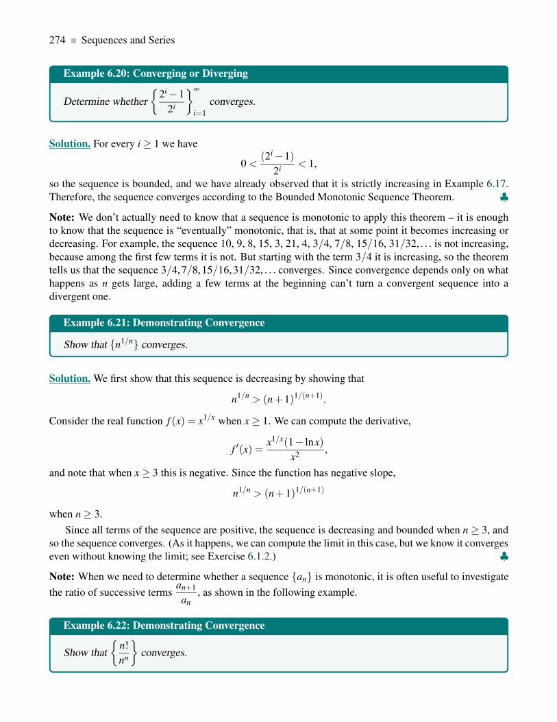
274 Sequences and Series
Example 6.20: Converging or Diverging
Determine whether
{
2i −1
2i
}∞
i=1
converges.
Solution. For every i ≥ 1 we have
0 <(2i −1)
2i< 1,
so the sequence is bounded, and we have already observed that it is strictly increasing in Example 6.17.
Therefore, the sequence converges according to the Bounded Monotonic Sequence Theorem. ♣Note: We don’t actually need to know that a sequence is monotonic to apply this theorem – it is enough
to know that the sequence is “eventually” monotonic, that is, that at some point it becomes increasing or
decreasing. For example, the sequence 10, 9, 8, 15, 3, 21, 4, 3/4, 7/8, 15/16, 31/32, . . . is not increasing,
because among the first few terms it is not. But starting with the term 3/4 it is increasing, so the theorem
tells us that the sequence 3/4,7/8,15/16,31/32, . . . converges. Since convergence depends only on what
happens as n gets large, adding a few terms at the beginning can’t turn a convergent sequence into a
divergent one.
Example 6.21: Demonstrating Convergence
Show that {n1/n} converges.
Solution. We first show that this sequence is decreasing by showing that
n1/n > (n+1)1/(n+1).
Consider the real function f (x) = x1/x when x ≥ 1. We can compute the derivative,
f ′(x) =x1/x(1− lnx)
x2,
and note that when x ≥ 3 this is negative. Since the function has negative slope,
n1/n > (n+1)1/(n+1)
when n ≥ 3.
Since all terms of the sequence are positive, the sequence is decreasing and bounded when n ≥ 3, and
so the sequence converges. (As it happens, we can compute the limit in this case, but we know it converges
even without knowing the limit; see Exercise 6.1.2.) ♣Note: When we need to determine whether a sequence {an} is monotonic, it is often useful to investigate
the ratio of successive termsan+1
an, as shown in the following example.
Example 6.22: Demonstrating Convergence
Show that
{
n!
nn
}
converges.

6.2. Series 275
Solution. If we look at the ratio of successive terms we see that:
an+1
an=
(n+1)!
(n+1)n+1
nn
n!=
(n+1)!
n!
nn
(n+1)n+1=
n+1
n+1
(
n
n+1
)n
=
(
n
n+1
)n
< 1.
Therefore an+1 < an, and so the sequence is decreasing. Since all terms are positive, it is also bounded,
and so it must converge. (Again it is possible to compute the limit; see Exercise 6.1.3.) ♣
Exercises for Section 6.1
Exercise 6.1.1 Graph the first 5 terms of the following sequences.
(a){
n2 −n}∞
n=0
(b)
{ √n√
n+1
}∞
n=0
(c)
{
en
n2
}∞
n=1
(d){ n
3n
}∞
n=1
Exercise 6.1.2 Compute limx→∞
x1/x.
Exercise 6.1.3 Use the Squeeze Theorem to show that limn→∞
n!
nn= 0.
Exercise 6.1.4 Determine whether the following sequences converge or diverge. In the case of conver-
gence, compute the limit.
(a) {n2 −n}∞n=0
(b)
{ √n√
n+1
}∞
n=0
(c)
{
en
n2
}∞
n=1
(d){ n
3n
}∞
n=1
(e){√
n+47−√
n}∞
n=0
(f)
{
n2 +1
(n+1)2
}∞
n=0
(g)
{
n+47√n2 +3n
}∞
n=1
(h)
{
2n
n!
}∞
n=0
6.2 Series
While much more can be said about sequences, we now turn to our principal interest, series. Recall that a
series, roughly speaking, is the sum of a sequence: If {an}∞n=0 is a sequence then we can construct a series

276 Sequences and Series
by adding up all the terms in the sequence:
∞
∑n=0
an = a0 +a1 +a2 + · · ·
Definition 6.23: Infinite Series
Given an infinite sequence {an}∞n=0, the sum
∞
∑n=0
an = a0 +a1 +a2 + . . .
is called an infinite series.
Associated with a series is a second sequence, called the sequence of partial sums {sn}∞n=0, where the
n-th partial sum sn always terminates with the n-th term an of the sequence:
s0 = a0, s1 = a0 +a1, s2 = a0 +a1 +a2, . . .
Definition 6.24: Sequence of Partial Sums
Given an infinite series∞
∑n=0
an, the sequence of partial sums is {sn}∞n=0, where the n-th partial
sum is defined as
sn =n
∑i=0
ai = a0 +a1 +a2 + · · ·+an.
Again, we are interested in the behaviour of the series, and whether its terms sum to a finite number or
not. We therefore define convergence and divergence for a series.
Definition 6.25: Convergence and Divergence of a Series
Given an infinite series∞
∑n=0
an, the series converges if the associated sequence of partial sums con-
verges; otherwise, the series diverges.
Definition 6.26: Geometric Series
If {kxn}∞n=0 is a geometric sequence, then the associated series ∑∞
i=0 kxi is called a geometric series.
Note: An infinite series∞
∑n=0
an can also be denoted by ∑n
an or ∑an, where it is understood that n is an
integer that runs over all admissible values of the index. However, if we are interested in the actual sum of
the series, then it is pertinent to identify the lower bound of the series.

6.2. Series 277
Theorem 6.27: Geometric Series Convergence
Given a geometric series∞
∑n=0
kxn with k 6= 0:
1. If |x|< 1, the series converges∞
∑n=0
kxn =k
1− x.
2. If |x| ≥ 1, the series diverges.
Proof.
A typical partial sum is
sn = k+ kx+ kx2 + kx3 + · · ·+ kxn = k(1+ x+ x2 + x3 + · · ·+ xn).
We note that for x 6= 1,
sn(1− x) = k(1+ x+ x2 + x3 + · · ·+ xn)(1− x)
= k(1+ x+ x2 + x3 + · · ·+ xn)1− k(1+ x+ x2 + x3 + · · ·+ xn−1 + xn)x
= k(1+ x+ x2 + x3 + · · ·+ xn − x− x2 − x3 −·· ·− xn − xn+1)
= k(1− xn+1)
so
sn(1− x) = k(1− xn+1)
sn = k1− xn+1
1− x.
1. If |x|< 1, limn→∞
xn = 0 so
limn→∞
sn = limn→∞
k1− xn+1
1− x= k
1
1− x.
Thus, when |x|< 1 the geometric series converges to k/(1− x).
2. (a) If |x|> 1, then
limn→∞
xn = ∞
and so the series diverges.
(b) If |x|= 1, then
|sn|=n
∑i=0
1 = n+1.
Therefore,
limn→∞
|sn|= limn→∞
(n+1) = ∞
and so the series diverges.

278 Sequences and Series
♣
Example 6.28: Summing a Geometric Series
Given the series∞
∑n=0
1
2n, determine the following:
(a) The partial sum sn. (b) The sum of the series.
Solution. We recognize that the series is geometric with k = 1 and x = 1/2.
(a) sn =1− (1/2)n+1
1−1/2=
2n+1 −1
2n= 2− 1
2n
(b)∞
∑n=0
1
2n=
1
1−1/2= 2.
♣
We began the chapter with the series∞
∑n=1
1
2n,
namely, the geometric series without the first term 1. Each partial sum of this series is 1 less than the
corresponding partial sum for the geometric series, so of course the limit is also one less than the value of
the geometric series, that is,∞
∑n=1
1
2n= 1.
It is not hard to see that the following theorem follows from Theorem 6.6.
Theorem 6.29: Series are Linear
Suppose that ∑an and ∑bn are convergent series, and c is a constant. Then
1. ∑can is convergent and ∑can = c∑an
2. ∑(an +bn) is convergent and ∑(an+bn) = ∑an +∑bn.
Note:
1. When c is non-zero, the converse of the first part of this theorem is also true. That is, if ∑can is
convergent, then ∑an is also convergent; if ∑can converges then 1c ∑can must converge.
2. On the other hand, the converse of the second part of the theorem is not true. For example, if an = 1
and bn =−1, then ∑an +∑bn = ∑0 = 0 converges, but each of ∑an and ∑bn diverges.

6.2. Series 279
In general, the sequence of partial sums sn is harder to understand and analyze than the sequence of
terms an, and it is difficult to determine whether series converge and if so to what. The following result
will let us deal with some simple cases easily.
Theorem 6.30: Divergence Test
If ∑an converges then limn→∞
an = 0.
Proof. Since ∑an converges, limn→∞
sn = L and limn→∞
sn−1 = L, because this really says the same thing but
“renumbers” the terms. By Theorem 6.6,
limn→∞
(sn − sn−1) = limn→∞
sn − limn→∞
sn−1 = L−L = 0.
But
sn − sn−1 = (a0 +a1 +a2 + · · ·+an)− (a0 +a1 +a2 + · · ·+an−1) = an,
so as desired limn→∞
an = 0. ♣
Note:
1. This theorem presents an easy Divergence Test when we use the contrapositive form: Given a series
∑an, if the limit limn→∞
an does not exist or has a value other than zero, the series diverges. This result
is captured in the next theorem called the n-th Term Test. Often, this theorem is referred to as the
Divergence Test.
2. Note well that the converse is not true: If limn→∞
an = 0 then the series does not necessarily converge.
One example is the so-called harmonic series, as will be shown in Example 6.33.
Theorem 6.31: n-th Term Test
If limn→∞
an 6= 0 or if the limit does not exist, then ∑an diverges.
Proof. Consider the statement of the theorem in contrapositive form:
If∞
∑n=1
an converges, then limn→∞
an = 0.
If sn are the partial sums of the series, then the assumption that the series converges gives us
limn→∞
sn = s
for some number s. Then
limn→∞
an = limn→∞
(sn − sn−1) = limn→∞
sn − limn→∞
sn−1 = s− s = 0.
♣

280 Sequences and Series
Example 6.32: Demonstrating Divergence
Show that∞
∑n=1
n
n+1diverges.
Solution. We compute the limit:
limn→∞
n
n+1= 1 6= 0.
Looking at the first few terms perhaps makes it clear that the series has no chance of converging:
1
2+
2
3+
3
4+
4
5+ · · ·
will just get larger and larger; indeed, after a bit longer the series starts to look very much like · · ·+1+1+1+1+ · · · , and of course if we add up enough 1’s we can make the sum as large as we desire. ♣
Example 6.33: Harmonic Series
Show that∞
∑n=1
1
ndiverges.
Solution. Here the theorem does not apply: limn→∞
1/n = 0, so it looks like perhaps the series converges.
Indeed, if you have the fortitude (or the software) to add up the first 1000 terms you will find that
1000
∑n=1
1
n≈ 7.49,
so it might be reasonable to speculate that the series converges to something in the neighborhood of 10.
But in fact the partial sums do go to infinity; they just get big very, very slowly. Consider the following:
1+1
2+
1
3+
1
4> 1+
1
2+
1
4+
1
4= 1+
1
2+
1
2
1+1
2+
1
3+
1
4+
1
5+
1
6+
1
7+
1
8> 1+
1
2+
1
4+
1
4+
1
8+
1
8+
1
8+
1
8= 1+
1
2+
1
2+
1
2
1+1
2+
1
3+ · · ·+ 1
16> 1+
1
2+
1
4+
1
4+
1
8+ · · ·+ 1
8+
1
16+ · · ·+ 1
16= 1+
1
2+
1
2+
1
2+
1
2and so on. By swallowing up more and more terms we can always manage to add at least another 1/2 to
the sum, and by adding enough of these we can make the partial sums as big as we like. In fact, it’s not
hard to see from this pattern that
1+1
2+
1
3+ · · ·+ 1
2n> 1+
n
2,
so to make sure the sum is over 100, for example, we’d add up terms until we get to around 1/2198, that
is, about 4 ·1059 terms. ♣

6.3. The Integral Test 281
Definition 6.34: Harmonic Series
A series of the form∞
∑n=1
1
n= 1+
1
2+
1
3+ · · ·+ 1
n+ . . .
is called a harmonic series.
Note: We will often make use of the fact that the first few (e.g. any finite number of) terms in a series
are irrelevant when determining whether it will converge. In other words,∞
∑n=0
an converges if and only if
∞
∑n=N
an converges for some N ≥ 1.
Exercises for Section 6.2
Exercise 6.2.1 Explain why the following series diverge.
(a)∞
∑n=1
n2
2n2 +1
(b)∞
∑n=1
5
21/n +14
(c)∞
∑n=1
3
n
Exercise 6.2.2 Compute the sum of the following series, if it converges.
(a)∞
∑n=0
(
4
(−3)n− 3
3n
)
(b)∞
∑n=0
(
3
2n+
4
5n
)
(c)∞
∑n=0
4n+1
5n
(d)∞
∑n=0
3n+1
7n+1
(e)∞
∑n=1
(
3
5
)n
(f)∞
∑n=1
3n
5n+1
6.3 The Integral Test
It is generally quite difficult, often impossible, to determine the value of a series exactly. In many cases
it is possible at least to determine whether or not the series converges, and so we will spend most of our
time on this problem.

282 Sequences and Series
If all of the terms an in a series are non-negative, then clearly the sequence of partial sums sn is
non-decreasing. This means that if we can show that the sequence of partial sums is bounded, the series
must converge. Many useful and interesting series have this property, and they are among the easiest to
understand. Let’s look at an example.
Example 6.35: Exploring Convergence Using an Integral
Show that∞
∑n=1
1
n2converges.
Solution. The terms 1/n2 are positive and decreasing, and since limx→∞
1/x2 = 0, the terms 1/n2 approach
zero. This means that the Divergence Test does not provide any information and we must find a different
method to deal with this series. We seek an upper bound for all the partial sums, that is, we want to find a
number N so that sn ≤N for every n. The upper bound is provided courtesy of integration, and is illustrated
in Figure 6.2.
A = 1
A = 1/4
1 2 3 4
1
x
y
Figure 6.2: Graph of y = 1/x2 with rectangles.
The figure shows the graph of y = 1/x2 together with some rectangles that lie completely below the
curve and that all have base length one. Because the heights of the rectangles are determined by the height
of the curve, the areas of the rectangles are 1/12, 1/22, 1/32, and so on—in other words, exactly the
terms of the series. The partial sum sn is simply the sum of the areas of the first n rectangles. Because the
rectangles all lie between the curve and the x-axis, any sum of rectangle areas is less than the corresponding
area under the curve, and so of course any sum of rectangle areas is less than the area under the entire curve.
Unfortunately, because of the asymptote at x = 0, the integral∫ ∞
01x2 is infinite, but we can deal with this
by separating the first term from the series and integrating from 1:
sn =n
∑i=1
1
i2= 1+
n
∑i=2
1
i2< 1+
∫ n
1
1
x2dx < 1+
∫ ∞
1
1
x2dx = 1+1 = 2,
recalling that we computed this improper integral in Section 2.7. Since the sequence of partial sums sn is

6.3. The Integral Test 283
increasing and bounded above by 2, we know that limn→∞
sn = L < 2, and so the series converges to some
number less than 2. In fact, it is possible, though difficult, to show that L = π2/6 ≈ 1.6. ♣
Example 6.36: Exploring Divergence Using an Integral
Why can the integral technique from Example 6.35 not be used with the series
∞
∑n=1
1
n?
Solution. We already know that ∑1/n diverges. What goes wrong if we try to apply the integral technique
to it? Here’s the calculation:
sn =1
1+
1
2+
1
3+ · · ·+ 1
n< 1+
∫ n
1
1
xdx < 1+
∫ ∞
1
1
xdx = 1+∞.
The problem is that the improper integral doesn’t converge. Note that this does not prove that ∑1/n
diverges, just that this particular technique fails to prove that it converges. ♣
A slight modification, however, allows us to prove in a second way that ∑1/n diverges.
Example 6.37: Alternate Method for Divergence of Harmonic Series
Use the idea of areas from Example 6.35 to show that the series
∞
∑n=1
1
n
diverges.
Solution. Consider a slightly altered version of Figure 6.2, shown in Figure 6.3.
A = 1
A = 1/2
A = 1/3
1 2 3 4
1
x
y
Figure 6.3: Graph of y = 1/x with rectangles.

284 Sequences and Series
This time the rectangles are above the curve, that is, each rectangle completely contains the corre-
sponding area under the curve. This means that
sn =1
1+
1
2+
1
3+ · · ·+ 1
n>
∫ n+1
1
1
xdx = lnx
∣
∣
∣
n+1
1= ln(n+1).
As n gets bigger, ln(n+1) goes to infinity, so the sequence of partial sums sn must also go to infinity, so
the harmonic series diverges.
The key fact in this example is that
limn→∞
∫ n+1
1
1
xdx =
∫ ∞
1
1
xdx = ∞.
♣
So these two examples taken together indicate that we can prove that a series converges or prove that
it diverges with a single calculation of an improper integral. This is known as the Integral Test, which we
state as a theorem.
Theorem 6.38: Integral Test
Suppose that f is a continuous, positive, and decreasing function of x on the infinite interval [1,∞)and that an = f (n). Then
∞
∑n=1
an and
∫ ∞
1f (x)dx
either both converge or both diverge.
Note: The lower bound in the Integral Test is arbitrary. We could have chosen any positive integer N as
the lower bound, since – as mentioned before – the first few (e.g. any finite number of) terms in a series
are irrelevant when determining whether it will converge.
The two examples we have seen are called p-series. A p-series is any series of the form ∑1/np.
Definition 6.39: p-Series
A series of the form∞
∑n=1
1
np= 1+
1
2p+
1
3p+ · · ·+ 1
np+ . . ., where p is a constant, is called a p-
series.
Theorem 6.40: p-Series Test
Given the p-series∞
∑n=1
1
np= 1+
1
2p+
1
3p+ · · ·+ 1
np+ · · · :
1. If p > 1, the series converges.
2. If p ≤ 1, the series diverges.

6.3. The Integral Test 285
Proof. We split the proof into three cases:
∫ ∞
1
1
xpdx = lim
R→∞
x1−p
1− p
∣
∣
∣
∣
R
1
= limR→∞
R1−p
1− p− 1
1− p.
1. If p > 1 then 1− p < 0 and limR→∞
R1−p = 0, so the integral converges.
2. If p < 1 then 1− p > 0 and limR→∞
R1−p = ∞, so the integral diverges.
3. If p = 1, we have the harmonic series, which we have already shown in two ways to be divergent.
♣
Example 6.41: p-Series Power of Three
Show that∞
∑n=1
1
n3converges.
Solution. We could of course use the Integral Test, but now that we have the theorem we may simply note
that this is a p-series with p > 1. ♣
Example 6.42: p-Series Power of Four
Show that∞
∑n=1
5
n4converges.
Solution. We know that if∞
∑n=1
1/n4 converges then∞
∑n=1
5/n4 also converges, by Theorem 6.29. Since
p = 4 > 1 we have that∞
∑n=1
1/n4 is a convergent p-series, and so∞
∑n=1
5/n4 converges also. ♣
Example 6.43: p-Series Square Root
Show that∞
∑n=1
5√n
diverges.
Solution. This also follows from Theorem 6.29: Since∞
∑n=1
1√n
is a p-series with p = 1/2 < 1, it diverges,
and so does∞
∑n=1
5√n
. ♣
Note: Since it is typically difficult to compute the value of a series exactly, a good approximation is
frequently required. In a real sense, a good approximation is only as good as we know it is, that is, while

286 Sequences and Series
an approximation may in fact be good, it is only valuable in practice if we can guarantee its accuracy to
some degree. This guarantee is usually easy to come by for series with decreasing positive terms.
Example 6.44: Approximating a p-Series
Approximate∞
∑n=1
1/n2 to within 0.01.
Solution. Referring to Figure 6.2, if we approximate the sum byN
∑n=1
1/n2, the size of the error we make is
the total area of the remaining rectangles, all of which lie under the curve 1/x2 from x = N to infinity. So
we know the true value of the series is larger than the approximation, and no bigger than the approximation
plus the area under the curve from N to infinity. Roughly, then, we need to find N so that
∫ ∞
N
1
x2dx < 1/100.
We can compute the integral:∫ ∞
N
1
x2dx =
1
N,
so if we choose N = 100 the error will be less than 0.01. Adding up the first 100 terms gives approxi-
mately 1.634983900. In fact, we can do a bit better. Since we know that the correct value is between our
approximation and our approximation plus the error (not minus), we can cut our error bound in half by
taking the value midway between these two values. If we take N = 50, we get a sum of 1.6251327 with an
error of at most 0.02, so the correct value is between 1.6251327 and 1.6451327, and therefore the value
halfway between these, 1.6351327, is within 0.01 of the correct value. We have mentioned that the true
value of this series can be shown to be π2/6 ≈ 1.644934068 which is 0.0098 more than our approxima-
tion, and so (just barely) within the required error. Frequently approximations will be even better than the
“guaranteed” accuracy, but not always, as this example demonstrates. ♣
Exercises for Section 6.3
Exercise 6.3.1 Determine whether each series converges or diverges.
(a)∞
∑n=1
1
nπ/4
(b)∞
∑n=1
n
n2 +1
(c)∞
∑n=1
lnn
n2
(d)∞
∑n=1
1
n2 +1
(e)∞
∑n=1
1
en
(f)∞
∑n=1
n
en

6.4. Alternating Series 287
(g)∞
∑n=2
1
n lnn(h)
∞
∑n=2
1
n(lnn)2
Exercise 6.3.2 Find an N so that each series is approximated to within the given error.
(a)∞
∑n=1
1
n4, 0.005
(b)∞
∑n=0
1
en, 10−4
(c)∞
∑n=1
lnn
n2, 0.005
(d)∞
∑n=2
1
n(lnn)2, 0.005
6.4 Alternating Series
Next we consider series with both positive and negative terms, but in a regular pattern: they alternate signs.
For example:
•∞
∑n=1
(−1)n−1 2
n+1= 1− 2
3+
2
4− 2
5+ . . .
•∞
∑n=1
(−1)n 2
n+1=−1+
2
3− 2
4+
2
5− . . .
•∞
∑n=0
(−1)n2n = 1−2+4−8+ . . .
•∞
∑n=4
(−1)n−1 n
n+2=−4
6+
5
7− 6
8+
7
9− . . .
Definition 6.45: Alternating Series
An alternating series has the form
∑(−1)nan
where an are all positive and the first index is arbitrary.
Note: An alternating series can start with a positive or negative term, i.e. the first index can be any
non-negative integer.
A well-known example of an alternating series is the alternating harmonic series:

288 Sequences and Series
Definition 6.46: Alternating Harmonic Series
A series of the form
∞
∑n=1
(−1)n−1
n= 1− 1
2+
1
3− 1
4+ · · ·+ (−1)n−1
n+ . . .
is called an alternating harmonic series.
In the alternating harmonic series the magnitude of the terms decrease, that is, |an| forms a decreasing
sequence, although this is not required in an alternating series. Recall that for a series with positive terms,
if the limit of the terms is not zero, the series cannot converge; but even if the limit of the terms is zero, the
series still may not converge. It turns out that for alternating series, the series converges exactly when the
limit of the terms is zero. In Figure 6.4, we illustrate what happens to the partial sums of the alternating
harmonic series. Because the sizes of the terms an are decreasing, the odd partial sums s1, s3, s5, and so
on, form a decreasing sequence that is bounded below by s2, so this sequence must converge. Likewise,
the even partial sums s2, s4, s6, and so on, form an increasing sequence that is bounded above by s1, so
this sequence also converges. Since all the even numbered partial sums are less than all the odd numbered
ones, and since the “jumps” (that is, the ai terms) are getting smaller and smaller, the two sequences must
converge to the same value, meaning the entire sequence of partial sums s1,s2,s3, . . . converges as well.
14
1 = s1 = a1
a2 =−12
s2 =12
a3
s3
a4
s4
a5
s5
a6
s6
..................................................................................................................................................................................................................................................................................................................................................................................................................................................................................................................................................................
............
................................................................................................................................................................................................................................................................................................................................................................................
............
.......................................................................................................................................................................................................................................................................................
............
..................................................................................................................................................................................................................................
............
..............................................................................................................................................................................................
............
Figure 6.4: The alternating harmonic series.
The same argument works for any alternating sequence with terms that decrease in absolute value. The
Alternating Series Test is worth calling a theorem.
Theorem 6.47: Alternating Series Test
Suppose that {an}∞n=1 is a non-increasing sequence of positive numbers and lim
n→∞an = 0. Then the
alternating series∞
∑n=1
(−1)n−1an converges.
Proof. The odd-numbered partial sums, s1,s3,s5, . . . ,s2k+1, . . ., form a non-increasing sequence, because
s2k+3 = s2k+1 − a2k+2 + a2k+3 ≤ s2k+1, since a2k+2 ≥ a2k+3. This sequence is bounded below by s2, so
it must converge, to some value L. Likewise, the partial sums s2,s4,s6, . . . ,s2k, . . ., form a non-decreasing
sequence that is bounded above by s1, so this sequence also converges, to some value M. Since limn→∞
an = 0
6.4. Alternating Series 289
and s2k+1 = s2k +a2k+1,
L = limk→∞
s2k+1 = limk→∞
(s2k +a2k+1) = limk→∞
s2k + limk→∞
a2k+1 = M+0 = M,
so L=M; the two sequences of partial sums converge to the same limit, and this means the entire sequence
of partial sums also converges to L. ♣
Another useful fact is implicit in this discussion. Suppose that
L =∞
∑n=1
(−1)n−1an
and that we approximate L by a finite part of this sum, say
L ≈N
∑n=1
(−1)n−1an.
Because the terms are decreasing in size, we know that the true value of L must be between this approxi-
mation and the next one, that is, between
N
∑n=1
(−1)n−1an andN+1
∑n=1
(−1)n−1an.
Depending on whether N is odd or even, the second will be larger or smaller than the first.
Example 6.48: Approximating a Series
Approximate the sum of the alternating harmonic series to within 0.05.
Solution. We need to go to the point at which the next term to be added or subtracted is 1/10. Adding up
the first nine and the first ten terms we get approximately 0.746 and 0.646. These are 1/10 apart, so the
value halfway between them, 0.696, is within 0.05 of the correct value. ♣
Note: We have considered alternating series with first index 1, and in which the first term is positive, but
a little thought shows this is not crucial. The same test applies to any similar series, such as∞
∑n=0
(−1)nan,
∞
∑n=1
(−1)nan,∞
∑n=17
(−1)nan, etc.
Exercises for Section 6.4
Exercise 6.4.1 Determine whether the following series converge or diverge.

290 Sequences and Series
(a)∞
∑n=1
(−1)n−1
2n+5
(b)∞
∑n=4
(−1)n−1
√n−3
(c)∞
∑n=1
(−1)n−1 n
3n−2
(d)∞
∑n=1
(−1)n−1 lnn
n
Exercise 6.4.2 Approximate each series to within the given error.
(a)∞
∑n=1
(−1)n−1 1
n3, 0.005 (b)
∞
∑n=1
(−1)n−1 1
n4, 0.005
6.5 Comparison Test
As we begin to compile a list of convergent and divergent series, new ones can sometimes be analyzed by
comparing them to ones that we already understand.
Example 6.49: Convergence by Comparison
Does∞
∑n=2
1
n2 lnnconverge?
Solution. The obvious first approach, based on what we know, is the Integral Test. Unfortunately, we
can’t compute the required antiderivative. But looking at the series, it would appear that it must converge,
because the terms we are adding are smaller than the terms of a p-series, that is,
1
n2 lnn<
1
n2,
when n ≥ 3. Since adding up the terms 1/n2 doesn’t get “too big”, the new series “should” also converge.
Let’s make this more precise.
The series∞
∑n=2
1
n2 lnnconverges if and only if
∞
∑n=3
1
n2 lnnconverges—all we’ve done is dropped the
initial term. We know that∞
∑n=3
1
n2converges. Looking at two typical partial sums:
sn =1
32 ln3+
1
42 ln4+
1
52 ln5+ · · ·+ 1
n2 lnn<
1
32+
1
42+
1
52+ · · ·+ 1
n2= tn.
Since the p-series converges, say to L, and since the terms are positive, tn < L. Since the terms of the new
series are positive, the sn form an increasing sequence and sn < tn < L for all n. Hence the sequence {sn}is bounded and so converges. ♣
6.5. Comparison Test 291
Like the Integral Test, the so-called Comparison Test can be used to show both convergence and
divergence. In the case of the Integral Test, a single calculation will confirm whichever is the case. To use
the Comparison Test we must first have a good idea as to convergence or divergence and pick the sequence
for comparison accordingly.
Example 6.50: Divergence by Comparison
Does∞
∑n=2
1√n2 −3
converge?
Solution. We observe that the −3 should have little effect compared to the n2 inside the square root.
Therefore, we guess that the terms are enough like 1/√
n2 = 1/n so that the series should diverge. This
analysis leads us to apply the Comparison Test based on the harmonic series. We note that
1√n2 −3
>1√n2
=1
n,
so that
sn =1√
22 −3+
1√32 −3
+ · · ·+ 1√n2 −3
>1
2+
1
3+ · · ·+ 1
n= tn,
where tn is 1 less than the corresponding partial sum of the harmonic series because we start at n = 2
instead of n = 1. Since limn→∞
tn = ∞, limn→∞
sn = ∞ as well. Hence, the given series diverges. ♣
For reference, we summarize the Comparison Test in a theorem.
Theorem 6.51: Comparison Test for Series
Suppose that an and bn are non-negative for all n and that an ≤ bn when n ≥ N, for some N.
1. If∞
∑n=0
bn converges, then∞
∑n=0
an also converges.
2. If∞
∑n=0
an diverges, then∞
∑n=0
bn also converges.
Note:
1. Sometimes, even when the Integral Test applies, comparison to a known series is easier, so it’s
generally a good idea to think about doing a comparison before doing the Integral Test.
2. The general approach is this: If you believe that a new series is convergent, attempt to find a conver-
gent series whose terms are larger than the terms of the new series; if you believe that a new series
is divergent, attempt to find a divergent series whose terms are smaller than the terms of the new
series.

292 Sequences and Series
Example 6.52: Applying the Comparison Test
Does∞
∑n=1
1√n2 +3
converge?
Solution. Just as in the last example, we guess that this is very much like the harmonic series and so
diverges. Unfortunately,1√
n2 +3<
1
n,
so we can’t compare the series directly to the harmonic series. A little thought leads us to
1√n2 +3
>1√
n2 +3n2=
1
2n,
so if ∑1/(2n) diverges then the given series diverges. But since ∑1/(2n) = (1/2)∑1/n, Theorem 6.29
implies that it does indeed diverge. ♣
Example 6.53: Integral Test or Comparison Test
Does∞
∑n=2
|sinn|n2
converge?
Solution. We can’t apply the Integral Test here, because the terms of this series are not decreasing. Just as
in Example 6.49, however,|sinn|
n2≤ 1
n2,
because |sinn| ≤ 1. Once again, the partial sums
sn =n
∑i=2
|sin i|i2
are non-decreasing and bounded above by
tn =n
∑i=2
1
i2< L,
where L is the sum of the p-series∞
∑n=2
1
n2. So the given series converges. ♣
Exercises for Section 6.5
Exercise 6.5.1 Determine whether the series converge or diverge.

6.6. Absolute and Conditional Convergence 293
(a)∞
∑n=1
1
2n2 +3n+5
(b)∞
∑n=2
1
2n2 +3n−5
(c)∞
∑n=1
1
2n2 −3n−5
(d)∞
∑n=1
3n+4
2n2 +3n+5
(e)∞
∑n=1
3n2 +4
2n2 +3n+5
(f)∞
∑n=1
lnn
n
(g)∞
∑n=1
lnn
n3
(h)∞
∑n=2
1
lnn
(i)∞
∑n=1
3n
2n +5n
(j)∞
∑n=1
3n
2n +3n
6.6 Absolute and Conditional Convergence
Roughly speaking there are two ways for a series to converge: As in the case of ∑1/n2, the individual terms
get small very quickly, so that the sum of all of them stays finite, or, as in the case of ∑(−1)n−1/n, the
terms don’t get small fast enough (∑1/n diverges), but a mixture of positive and negative terms provides
enough cancellation to keep the sum finite. You might guess from what we’ve seen that if the terms
get small fast enough that the sum of their absolute values converges, then the series will still converge
regardless of which terms are actually positive or negative. This leads us to the following theorem.
Theorem 6.54: Absolute Convergence Test
If∞
∑n=0
|an| converges, then∞
∑n=0
an converges.
Proof. Note that 0 ≤ an + |an| ≤ 2|an| so by the Comparison Test∞
∑n=0
(an+ |an|) converges. Since
∞
∑n=0
(an+ |an|)−∞
∑n=0
|an|=∞
∑n=0
an + |an|− |an|=∞
∑n=0
an,
by Theorem 6.29, the conclusion follows. ♣
Note:
1. Intuitively, this theorem says that it is (potentially) easier for ∑an to converge than for ∑ |an| to
converge, because terms may partially cancel in the first series.

294 Sequences and Series
2. So given a series ∑an with both positive and negative terms, you should first ask whether ∑ |an|converges. This may be an easier question to answer, because we have tests that apply specifically
to series with non-negative terms.
• If ∑ |an| converges then you know that ∑an converges as well.
• If ∑ |an| diverges then it still may be true that ∑an converges, but you will need to use other
techniques to decide.
If ∑ |an| converges we say that ∑an converges absolutely. To say that ∑an converges absolutely is to
say that the terms of the series get small (in absolute value) quickly enough to guarantee that the series
converges, regardless of whether any of the terms cancel each other. For example∞
∑n=1
(−1)n−1 1
n2converges
absolutely.
Definition 6.55: Absolutely Convergent
Given a series∞
∑n=1
an. If the corresponding series∞
∑n=1
|an| converges, then∞
∑n=1
an converges abso-
lutely.
If ∑an converges but ∑ |an| does not, we say that ∑an converges conditionally. Recall that the al-
ternating harmonic series∞
∑n=1
(−1)n−1
nconverges, but that the corresponding series of absolute values,
namely the harmonic series∞
∑n=1
1
n, diverges. Hence, the alternating harmonic series is conditionally con-
vergent.
Definition 6.56: Conditionally Convergent
Given a series∞
∑n=1
an. If∞
∑n=1
an converges, but the corresponding series∞
∑n=1
|an| does not converge,
then∞
∑n=1
an converges conditionally.
Note: Instead of writing that a series converges absolutely (or conditionally), we may also use the expres-
sion the series is absolutely (or conditionally) convergent.
Example 6.57: Absolutely Convergent, Conditionally Convergent, or Divergent
Does∞
∑n=2
sinn
n2converge? If so, how?
Solution. In Example 6.53 we saw that∞
∑n=2
|sinn|n2
converges, so the given series converges absolutely.
♣

6.6. Absolute and Conditional Convergence 295
Example 6.58: Absolutely Convergent, Conditionally Convergent, or Divergent
Does∞
∑n=0
(−1)n 3n+4
2n2 +3n+5converge? If so, how?
Solution. We begin by analyzing the corresponding series of absolute values, where
an =3n+4
2n2 +3n+5.
Looking at the leading terms in the numerator and denominator of an, we speculate to compare this series
with the harmonic series:
Left side Right side
1
n
3n+4
2n2 +3n+5
2n2 +3n+5 n(3n+4)
2n2 +3n+5 3n2 +4n
5 n2 +n
Indeed, n2 +n > 5 for n > 1, and therefore this series diverges since the harmonic series diverges. So if
the original series converges, it does so conditionally.
To test for convergence, we apply the Alternating Series Test:
1. Clearly, an =3n+4
2n2 +3n+5is positive for all n ≥ 0.
2. limn→∞
3n+4
2n2 +3n+5= 0.
3. If we let f (x) =3x+4
2x2 +3x+5then f ′(x) = − 6x2 +16x−3
(2x2 +3x+5)2, and it is not hard to see that this is
negative for x ≥ 1, so the sequence{
3n+42n2+3n+5
}∞
n=0is decreasing.
Thus, the series∞
∑n=0
(−1)n 3n+4
2n2 +3n+5converges by the Alternating Series Test, and we conclude that the
series converges conditionally. ♣
Exercises for Section 6.6
Exercise 6.6.1 Determine whether each series converges absolutely, converges conditionally, or diverges.

296 Sequences and Series
(a)∞
∑n=1
(−1)n−1 1
2n2 +3n+5
(b)∞
∑n=1
(−1)n−1 3n2 +4
2n2 +3n+5
(c)∞
∑n=1
(−1)n−1 lnn
n
(d)∞
∑n=1
(−1)n−1 lnn
n3
(e)∞
∑n=2
(−1)n 1
lnn
(f)∞
∑n=0
(−1)n 3n
2n +5n
(g)∞
∑n=0
(−1)n 3n
2n +3n
(h)∞
∑n=1
(−1)n−1 arctann
n
6.7 The Ratio and Root Tests
Does the series∞
∑n=0
n5
5nconverge? It is possible, but a bit unpleasant, to approach this with the Integral Test
or the Comparison Test, but there is an easier way. Consider what happens as we move from one term to
the next in this series:
· · ·+ n5
5n+
(n+1)5
5n+1+ · · ·
The denominator goes up by a factor of 5, 5n+1 = 5 · 5n, but the numerator goes up by much less:
(n+1)5 = n5 +5n4 +10n3 +10n2 +5n+1, which is much less than 5n5 when n is large, because 5n4 is
much less than n5. So we might guess that in the long run it begins to look as if each term is 1/5 of the
previous term. We have seen series that behave like this: The geometric series.
∞
∑n=0
1
5n=
5
4,
So we might try comparing the given series to some variation of this geometric series. This is possible,
but a bit messy. We can in effect do the same thing, but bypass most of the unpleasant work.
The key is to notice that
limn→∞
an+1
an= lim
n→∞
(n+1)5
5n+1
5n
n5= lim
n→∞
(n+1)5
n5
1
5= 1 · 1
5=
1
5.
This is really just what we noticed above, done a bit more formally: in the long run, each term is one
fifth of the previous term. Now pick some number between 1/5 and 1, say 1/2. Because
limn→∞
an+1
an=
1
5,
then when n is big enough, say n ≥ N for some N,

6.7. The Ratio and Root Tests 297
an+1
an<
1
2so an+1 <
an
2.
So aN+1 < aN/2, aN+2 < aN+1/2 < aN/4, aN+3 < aN+2/2 < aN/8, and so on. The general form is
aN+k < aN/2k. So if we look at the series
∞
∑k=0
aN+k = aN +aN+1 +aN+2 +aN+3 + · · ·+aN+k + · · · ,
its terms are less than or equal to the terms of the sequence
aN +aN
2+
aN
4+
aN
8+ · · ·+ aN
2k+ · · ·=
∞
∑k=0
aN
2k= 2aN .
So by the Comparison Test,∞
∑k=0
aN+k converges, and this means that∞
∑n=0
an converges, since we’ve just
added the fixed number a0 +a1 + · · ·+aN−1.
Under what circumstances could we do this? The crucial part was that the limit of an+1/an, say L,
was less than 1 so that we could pick a value r so that L < r < 1. The fact that L < r (in our example
1/5 < 1/2) means that we can compare the series ∑an to ∑rn, and the fact that r < 1 guarantees that ∑rn
converges. That’s really all that is required to make the argument work.
Theorem 6.59: Ratio Test
Given a series ∑an with positive terms and limn→∞
an+1
an= L:
1. If L < 1, then the series converges.
2. If L > 1, then the series diverges.
3. If L = 1, then this test gives no information.
Proof. The example above essentially proves the first part of this, if we simply replace 1/5 by L and 1/2
by r. Suppose that L > 1, and pick r so that 1 < r < L. Then for n ≥ N, for some N,
|an+1||an|
> r and |an+1|> r|an|.
This implies that |aN+k| > rk|aN|, but since r > 1 this means that limk→∞
|aN+k| 6= 0, which means also
that limn→∞
an 6= 0. By the Divergence Test, the series diverges.
To see that we get no information when L = 1, we need to exhibit two series with L = 1, one that
converges and one that diverges. The series ∑1/n2 and ∑1/n provide a simple example. ♣
Note:
1. The Ratio Test is particularly useful for series involving factorials and exponentials.

298 Sequences and Series
2. Absolute Convergence:
• In general, we require a series to just have non-zero terms
• Then we consider the absolute values of the terms: limn→∞
∣
∣
∣
∣
an+1
an
∣
∣
∣
∣
= L
• This means we are testing for absolute convergence.
Example 6.60: Factorials and Ratio Test
Analyze∞
∑n=0
5n
n!.
Solution.
limn→∞
5n+1
(n+1)!
n!
5n= lim
n→∞
5n+1
5n
n!
(n+1)!= lim
n→∞5
1
(n+1)= 0.
Since 0 < 1, the series converges. ♣
A similar argument to the one used for the Ratio Test justifies a related test that is occasionally easier
to apply, namely the so-called Root Test.
Theorem 6.61: Root Test
Given a series ∑an with positive terms and limn→∞
(an)1/n = L:
1. If L < 1, then the series converges.
2. If L > 1, then the series diverges.
3. If L = 1, then this test gives no information.
The proof of the Root Test is actually easier than that of the Ratio Test, and is left as an exercise.
Example 6.62: Exponentials and Root Test
Analyze∞
∑n=0
5n
nn.
Solution. The Ratio Test turns out to be a bit difficult on this series (try it). Using the Root Test:
limn→∞
(
5n
nn
)1/n
= limn→∞
(5n)1/n
(nn)1/n= lim
n→∞
5
n= 0.
Since 0 < 1, the series converges. ♣
Note:

6.8. Power Series and Polynomial Approximation 299
1. The Root Test is frequently useful for series involving exponentials.
2. Absolute Convergence:
• In general, we require a series to just have non-zero terms
• Then we consider the absolute values of the terms: limn→∞
(|an|)1/n = L
• This means we are testing for absolute convergence.
Exercises for Section 6.7
Exercise 6.7.1 Compute the following limit for the given series.
(a) limn→∞
|an+1/an| for ∑1/n2
(b) limn→∞
|an+1/an| for ∑1/n
(c) limn→∞
|an|1/n for ∑1/n2
(d) limn→∞
|an|1/n for ∑1/n
Exercise 6.7.2 Determine whether the series converge.
(a)∞
∑n=0
(−1)n 3n
5n
(b)∞
∑n=1
n!
nn
(c)∞
∑n=1
n5
nn
(d)∞
∑n=1
(n!)2
nn
6.8 Power Series and Polynomial Approximation
In this chapter we have a closer look at so-called power series, which arise in the study of analytic func-
tions. A power series is basically an infinite degree polynomial that represents some function. Since we
know a lot more about polynomial functions than arbitrary functions, this allows us to readily differentiate,
integrate, and approximate some functions using power series.
6.8.1. Power Series
Recall that the sum of a geometric series can be expressed using the simple formula:
∞
∑n=0
kxn =k
1− x,

300 Sequences and Series
if |x|< 1, and that the series diverges when |x| ≥ 1. At the time, we thought of x as an unspecified constant,
but we could just as well think of it as a variable, in which case the series
∞
∑n=0
kxn
is a function, namely, the function k/(1− x), as long as |x| < 1: Looking at this from the opposite per-
spective, this means that the function k/(1− x) can be represented as the sum of an infinite series. Why
would this be useful? While k/(1− x) is a reasonably easy function to deal with, the more complicated
representation ∑kxn does have some advantages: it appears to be an infinite version of one of the simplest
function types – a polynomial. Later on we will investigate some of the ways we can take advantage of
this ‘infinite polynomial’ representation, but first we should ask if other functions can even be represented
this way.
The geometric series has a special feature that makes it unlike a typical polynomial—the coefficients
of the powers of x are all the same, namely k. We will need to allow more general coefficients if we are to
get anything other than the geometric series.
Definition 6.63: Power Series Centred Around Zero
A power series is a series of the form∞
∑n=0
anxn,
where the coefficients an are real numbers.
Note:
1. As we did in the section on sequences, we can think of the an as being a function a(n) defined on
the non-negative integers.
2. It is important to remember that the an do not depend on x.
Example 6.64: Power Series Convergence
Determine the values of x for which the power series∞
∑n=1
xn
nconverges.
Solution. We can investigate convergence using the Ratio Test:
limn→∞
|x|n+1
n+1
n
|x|n = limn→∞
|x| n
n+1= |x|.
Thus when |x|< 1 the series converges and when |x|> 1 it diverges, leaving only two values in doubt.
When x = 1 the series is the harmonic series and diverges; when x = −1 it is the alternating harmonic
series (actually the negative of the usual alternating harmonic series) and converges. Thus, we may think
of∞
∑n=1
xn
nas a function from the interval [−1,1) to the real numbers. ♣

6.8. Power Series and Polynomial Approximation 301
A bit of thought reveals that the Ratio Test applied to a power series will always have the same nice
form. In general, we will compute
limn→∞
|an+1||x|n+1
|an||x|n= lim
n→∞|x| |an+1|
|an|= |x| lim
n→∞
|an+1||an|
= L|x|,
assuming that lim |an+1|/|an| exists:
• Then the series converges if L|x| < 1, that is, if |x| < 1/L, and diverges if |x| > 1/L. Only the two
values x =±1/L require further investigation. The value 1/L is called the radius of convergence.
• Thus the series will always define a function on the interval (−1/L,1/L), that perhaps will extend
to one or both endpoints as well. This interval is referred to as the interval of convergence, and is
essentially the domain of the power series.
Note: Two special cases deserve mention:
1. If L = 0 the limit is 0 no matter what value x takes, so the series converges for all x and the function
is defined for all real numbers.
2. If L = ∞, then no matter what value x takes the limit is infinite and the series converges only when
x = 0.
We can make these ideas a bit more general. Consider the series
∞
∑n=0
(x+2)n
3n
This looks a lot like a power series, but with (x+2)n instead of xn. Let’s try to determine the values of x
for which it converges. This is just a geometric series, so it converges when
|x+2|/3 < 1
|x+2|< 3
−3 < x+2 < 3
−5 < x < 1.
So the interval of convergence for this series is (−5,1). The centre of this interval is at −2, which is
at distance 3 from the endpoints, so the radius of convergence is 3, and we say that the series is centred at
−2.
Interestingly, if we compute the sum of the series we get
∞
∑n=0
(
x+2
3
)n
=1
1− x+23
=3
1− x.
Multiplying both sides by 1/3 we obtain
∞
∑n=0
(x+2)n
3n+1=
1
1− x,

302 Sequences and Series
which we recognize as being equal to∞
∑n=0
xn,
so we have two series with the same sum but different intervals of convergence.
This leads to the following definition:
Definition 6.65: Power Series Centred Around a
A power series centred at a has the form
∞
∑n=0
an(x−a)n,
where the centre a and coefficients an are real numbers.
Note: The power series centred at zero given in Definition 6.63 is a special case of the above definition
when a = 0.
Convergence of a Power Series
Given a power series ∑an(x−a)n and its radius of convergence R, the series behaves in one of three
ways:
1. The series converges absolutely for x with |x−a| < R, it diverges for x with |x−a| > R, and
at x = a−R and x = a+R further investigation is needed.
2. When R = ∞, the series converges absolutely for every x.
3. When R = 0, the series converges at x = a and diverges everywhere else.
Example 6.66: Interval of Convergence
Given the power series∞
∑n=0
(−1)nn(x−2)n
3n
determine the following:
(a) radius of convergence (b) interval of convergence
Solution. Obviously, the series converges for x = 2. To determine all values of x for which the series

6.8. Power Series and Polynomial Approximation 303
converges, we begin by applying the Ratio Test:
L = limn→∞
∣
∣
∣
∣
an+1
an
∣
∣
∣
∣
= limn→∞
∣
∣
∣
∣
(−1)n+1(n+1)(x−2)n+1
3n+1
3n
(−1)nn(x−2)n
∣
∣
∣
∣
= limn→∞
∣
∣
∣
∣
(n+1)(x−2)
3n
∣
∣
∣
∣
= |x−2| limn→∞
n+1
3n
=1
3|x−2|
(a) By the Ratio Test, the radius of convergence is R = 3.
(b) We now determine the interval of convergence. By the Ratio Test, the series converges absolutely if
L < 1:
1
3|x−2|< 1
=⇒ |x−2|< 3
=⇒ −3 < x−2 < 3
=⇒ −1 < x < 5
The series diverges if L > 1, i.e. x <−1 and x > 5.
Let us now look at the case when L = 1, which means investigating the behaviour of the series at
endpoints x =−1 and x = 5:
Case x =−1: Then the series becomes
∞
∑n=0
(−1)nn(−1−2)n
3n=
∞
∑n=0
(−1)2nn =∞
∑n=0
n.
Since limn→∞
n = ∞ 6= 0, this series is divergent by the n-th Term Test (Divergence Test).
Case x = 5: Then the series becomes
∞
∑n=0
(−1)nn(5−2)n
3n=
∞
∑n=0
(−1)nn.
Since limn→∞
(−1)nn does not exist, this series is also divergent by the n-th Term Test (Divergence
Test).
Thus, the interval of convergence for the given power series is x ∈ (−1,5).
♣

304 Sequences and Series
Example 6.67: Interval of Convergence
Given the power series∞
∑n=1
(n+1)!(x+3)n
determine the following:
(a) radius of convergence (b) interval of convergence
Solution. Obviously, the series converges for x = −3. To determine all values of x for which the series
converges, we begin by applying the Ratio Test:
L = limn→∞
∣
∣
∣
∣
an+1
an
∣
∣
∣
∣
= limn→∞
∣
∣
∣
∣
(n+2)!(x+3)n+1
(n+1)!(x+3)n
∣
∣
∣
∣
= |x+3| limn→∞
(n+1) = ∞,
provided that x 6=−3. Therefore, this series will only converge for x = 3.
(a) The radius of convergence is R = 0.
(b) The interval of convergence is x =−3, which is just one point.
♣
Exercises for Section 6.8.1
Exercise 6.8.1 Find the radius and interval of convergence for each series. In part c), do not attempt to
determine whether the endpoints are in the interval of convergence.
(a)∞
∑n=0
nxn
(b)∞
∑n=0
xn
n!
(c)∞
∑n=1
n!
nn(x−2)n
(d)∞
∑n=1
(n!)2
nn(x−2)n
(e)∞
∑n=1
(x+5)n
n(n+1)
(f)∞
∑n=1
n!
nnxn

6.8. Power Series and Polynomial Approximation 305
6.8.2. Calculus with Power Series
We now know that some functions can be expressed as power series, which look like infinite polynomials.
In fact, there are many extremely useful functions that cannot be represented using the usual elementary
functions, but they can be represented using a power series. For example, the Bessel functions and hy-
pergeometric functions which are important in such fields as engineering, physics and acoustics. Since it
is easy to find derivatives and integrals of polynomials, we might hope that we can take derivatives and
integrals of power series in an analogous way. In fact we can, as stated in the following theorem, which
we will not prove here.
Theorem 6.68: Differentiation and Integration of a Power Series
Suppose the power series f (x) =∞
∑n=0
an(x−a)n has radius of convergence R.
1. The derivative of f is the term by term differentiation of the power series:
f ′(x) =∞
∑n=1
nan(x−a)n−1
with radius of convergence R.
2. The integral of f is the term by term integration of the power series:
∫
f (x)dx =C+∞
∑n=0
an
n+1(x−a)n+1
with radius of convergence R.
Note: The process of differentiation and integration allows us to create further power series representations
of functions.
Example 6.69: Power Series Representation
Given f (x) = ln |1− x|:
(a) Find a power series representation of f .
(b) Use the first seven terms of this series to approximate ln(3/2).
(c) Approximate ln(9/4).
Solution.
(a) We recall that the derivative of ln |1− x| is 11−x , and so we start with the geometric series:
1
1− x=
∞
∑n=0
xn

306 Sequences and Series
when |x|< 1. Next, we integrate to obtain the function f :
∫
1
1− xdx =− ln |1− x|=
∞
∑n=0
1
n+1xn+1
f (x) = ln |1− x|=∞
∑n=0
− 1
n+1xn+1,
when |x| < 1. The series does not converge when x = 1, since ∑∞n=0− 1
n+1(1)n+1 = −∑∞
n=11n is the
negative harmonic series. But the series does converge when x = −1, since ∑∞n=0− 1
n+1(−1)n+1 =
∑∞n=1
(−1)n+1
n is the alternating harmonic series. Therefore, the interval of convergence is [−1,1).
(b) We note that −1 ≤ x < 1 implies 0 < 1− x ≤ 2, and that 0 < 32 ≤ 2, so we need x =−1
2 . Then
ln(3/2) = ln |−(−1/2)|=∞
∑n=0
− 1
n+1
(
−1
2
)n+1
=∞
∑n=0
(−1)n+1
(n+1)2n+1.
Now we use the first seven terms to approximate ln(3/2):
ln(3/2)≈ 1
2− 1
8+
1
24− 1
64+
1
160− 1
384+
1
896=
909
2240≈ 0.406.
Because this is an alternating series with decreasing terms, we know that the true value is between
909/2240 and 909/2240−1/2048 = 29053/71680 ≈ .4053, so 0.4053 ≤ ln(3/2)≤ 0.406.
(c) With a bit of arithmetic, we can approximate values outside of the interval of convergence, such as
9/4 > 2. We can use the approximation we just computed, plus some rules for logarithms:
ln(9/4) = ln((3/2)2) = 2ln(3/2)≈ 0.812,
and using our bounds above,
0.8106 ≤ ln(9/4)≤ 0.812.
♣
Exercises for Section 6.8.2
Exercise 6.8.2 Find a series representation for
(a) ln2
(b) ln(9/2)
Exercise 6.8.3 Find a power series representation for the following functions.

6.8. Power Series and Polynomial Approximation 307
(a) 1/(1− x)2
(b) 2/(1− x)3
(c) 1/(1− x)3
(d)
∫
ln(1− x)dx
6.8.3. Maclaurin Series and Taylor Series
We have seen that some functions can be represented as series, which may give valuable information
about the function. So far, we have seen only those examples that result from manipulation of our one
fundamental example, the geometric series. We would like to start with a given function and produce a
series to represent it, if possible.
Suppose that f (x) =∞
∑n=0
anxn on some interval of convergence centred at 0. Then we know that we
can compute derivatives of f by taking derivatives of the terms of the series. Let’s compute the first few
derivatives and look for a pattern:
f ′(x) =∞
∑n=1
nanxn−1 = a1 +2a2x+3a3x2 +4a4x3 + · · ·
f ′′(x) =∞
∑n=2
n(n−1)anxn−2 = 2a2 +3 ·2a3x+4 ·3a4x2 + · · ·
f ′′′(x) =∞
∑n=3
n(n−1)(n−2)anxn−3 = 3 ·2a3+4 ·3 ·2a4x+ · · ·
By examining these it’s not hard to discern the general pattern. The kth derivative must be
f (k)(x) =∞
∑n=k
n(n−1)(n−2) · · ·(n− k+1)anxn−k
= k(k−1)(k−2) · · ·(2)(1)ak +(k+1)(k) · · ·(2)ak+1x
+(k+2)(k+1) · · ·(3)ak+2x2 + · · ·
We can express this more clearly by using factorial notation:
f (k)(x) =∞
∑n=k
n!
(n− k)!anxn−k = k!ak +(k+1)!ak+1x+
(k+2)!
2!ak+2x2 + · · ·
We can solve for ak by substituting x = 0 in the formula for f (k)(x):
f (k)(0) = k!ak +∞
∑n=k+1
n!
(n− k)!an0n−k = k!ak,

308 Sequences and Series
ak =f (k)(0)
k!.
Note that the original series for f yields f (0) = a0. So if a function f can be represented by a series, we
can easily find such a series. This leads us to the definition of the so-called Maclaurin series.
Definition 6.70: Maclaurin Series
Suppose a function f is defined at x= 0 and whose derivatives all exist at x= 0. Then the Maclaurin
series of f at x = 0 is given by
f (x) =∞
∑n=0
f (n)(0)
n!xn
= f (0)+ f ′(0)+f ′′(0)
2!x2 + · · ·+ f (n)(0)
n!xn + · · ·
Note: A warning is in order here. Given a function f we may be able to compute the Maclaurin series,
but that does not mean we have found a series representation for f . We still need to know where the
series converges, and if, where it converges, it converges to f (x). While for most commonly encountered
functions the Maclaurin series does indeed converge to f on some interval, this is not true of all functions,
so care is required.
Example 6.71: Maclaurin Series
Find the Maclaurin series for f (x) = 1/(1− x).
Solution. We need to compute the derivatives of f and hope to spot a pattern.
f (x) = (1− x)−1
f ′(x) = (1− x)−2
f ′′(x) = 2(1− x)−3
f ′′′(x) = 6(1− x)−4
f (4)(x) = 4!(1− x)−5
...
f (n)(x) = n!(1− x)−n−1
So
an =f (n)(0)
n!=
n!(1−0)−n−1
n!= 1
and the Maclaurin series is∞
∑n=0
1 · xn =∞
∑n=0
xn,
the geometric series with interval of convergence |x|< 1. ♣

6.8. Power Series and Polynomial Approximation 309
As a practical matter, if we are interested in using a series to approximate a function, we will need
some finite number of terms of the series. Even for functions with messy derivatives we can compute
these using computer software like Sage. If we want to describe a series completely, we would like to
be able to write down a formula for a typical term in the series. Fortunately, a few of the most important
functions are very easy.
Example 6.72: Maclaurin Series
Find the Maclaurin series for f (x) = sinx.
Solution. Computing the first few derivatives is simple: f ′(x) = cosx, f ′′(x) = −sinx, f ′′′(x) = −cosx,
f (4)(x) = sinx, and then the pattern repeats. The values of the derivative when x = 0 are: 1, 0, −1, 0, 1, 0,
−1, 0,. . . , and so the Maclaurin series is
x− x3
3!+
x5
5!−·· ·=
∞
∑n=0
(−1)n x2n+1
(2n+1)!.
We should always determine the radius of convergence:
limn→∞
|x|2n+3
(2n+3)!
(2n+1)!
|x|2n+1= lim
n→∞
|x|2(2n+3)(2n+2)
= 0,
so the series converges for every x. Since it turns out that this series does indeed converge to sinx every-
where, we have a series representation for sinx for every x. ♣
Sometimes the formula for the n-th derivative of a function f is difficult to discover, but a combination
of a known Maclaurin series and some algebraic manipulation leads easily to the Maclaurin series for f .
Example 6.73: Maclaurin Series
Find the Maclaurin series for f (x) = xsin(−x).
Solution. To get from sinx to xsin(−x) we substitute −x for x and then multiply by x. We can do the same
thing to the series for sinx:
x∞
∑n=0
(−1)n (−x)2n+1
(2n+1)!= x
∞
∑n=0
(−1)n(−1)2n+1 x2n+1
(2n+1)!=
∞
∑n=0
(−1)n+1 x2n+2
(2n+1)!.
♣
As we have seen, a power series can be centred at a point other than zero, and the method that produces
the Maclaurin series can also produce such series, which are referred to as Taylor series.

310 Sequences and Series
Definition 6.74: Taylor Series
Suppose a function f is defined at x = a and whose derivatives all exist at x = a. Then the Taylor
series of f centred at x = a is given by
f (x) =∞
∑n=0
f (n)(a)
n!(x−a)n
= f (a)+ f ′(a)(x−a)+f ′′(a)
2!(x−a)2 + · · ·+ f (n)(a)
n!(x−a)n + · · ·
Note: Notice that the Maclaurin series is a special case of the Taylor series when a = 0.
Example 6.75: Taylor Series
Find a Taylor series centred at −2 for f (x) = 1/(1− x).
Solution.
Method 1: We develop the series from scratch. Suppose f (x) =∞
∑n=0
an(x+ 2)n. We compute the k-th
derivatives of f and the power series representation to solve for an:
Using our work in Example 6.71, the k-th derivative of f (x) = 11−x is given by
f (k)(x) = k!(1− x)−k−1.
Based on our work at the beginning of this section, the k-th derivative of the power series representation
is given by∞
∑n=k
n
(n− k)!an(x+2)n−k.
Now we equate these two results to obtain the following equation:
k!(1− x)−k−1 =∞
∑n=k
n!
(n− k)!an(x+2)n−k
and substituting x =−2 we get k!3−k−1 = k!ak and ak = 3−k−1 = 1/3k+1, so the series is
∞
∑n=0
(x+2)n
3n+1.
Method 2: We use the formula for the Taylor series representation of f :
f (x) =∞
∑n=0
f (n)(−2)
n!(x+2)n.

6.8. Power Series and Polynomial Approximation 311
Now we compute the first few derivatives and evaluate them at x =−2 to deduce a pattern:
f (x) = (1− x)−1 f (−2) =1
3
f ′(x) = (1− x)−2 f ′(−2) =1
32
f ′′(x) = 2!(1− x)−3 f ′′(−2) =3!
34
f ′′′(x) = 3!(1− x)−4 f ′′′(−2) =3!
34
Hence, the n-th derivative evaluated at x =−2 is
f (n)(−2) =n!
3n+1,
and so, as before, the series is
∞
∑n=0
f (n)(−2)
n!(x+2)n =
∞
∑n=0
n!3n+1
n!(x+2)n =
∞
∑n=0
(x+2)n
3n+1.
♣
Example 6.76: Taylor Series
Given f (x) = ex, find the following:
(a) The Taylor series of f centred at 3. (b) The interval of convergence for the series.
Solution.
(a) We use the formula for the Taylor series representation of f :
f (x) =∞
∑n=0
f (n)(3)
n!(x−3)n
Since the derivative of f (x) = ex is again ex, we have that the n-th derivative evaluated at x =−3 is
f (n)(3) = e3,
and so the series is∞
∑n=0
f (n)(3)
n(x−3)n =
∞
∑n=0
e3
n!(x−3)n.

312 Sequences and Series
(b) We use the Ratio Test to determine the radius of convergence:
L = limn→∞
∣
∣
∣
∣
an+1
an
∣
∣
∣
∣
= limn→∞
∣
∣
∣
∣
e3(x−3)n+1
(n+1)!
n!
e3(x−3)n
∣
∣
∣
∣
= limn→∞
∣
∣
∣
∣
x−3
n+1
∣
∣
∣
∣
= |x−3| limn→∞
1
n+1
= 0
Hence, the radius of convergence is infinity, and so the series converges absolutely for every x, i.e.
the interval of convergence is (−∞,∞).
♣
Table 6.1 is a list of the five most common Maclaurin series and their interval of convergence.
Function Maclaurin series Interval of convergence
11−x
∞
∑n=0
xn (−1,1)
ex∞
∑n=0
1
n!xn (−∞,∞)
ln(1+ x)∞
∑n=1
(−1)n−1 xn
n(−1,1]
sin(x)∞
∑n=0
(−1)n x2n+1
(2n+1)!(−∞,∞)
cos(x)∞
∑n=0
(−1)n x2n
(2n)!(−∞,∞)
Table 6.1: Common Maclaurin series.
Exercises for Section 6.8.3
Exercise 6.8.4 For each function, find the Maclaurin series and the radius of convergence.

6.8. Power Series and Polynomial Approximation 313
(a) f (x) = cosx
(b) f (x) = ex
(c) f (x) =1
1+ x
(d) f (x) = sin(2x)
(e) f (x) =1√
1− x
Exercise 6.8.5 For each function, find the Taylor series centred at a and the radius of convergence.
(a) f (x) =1
x, a = 5
(b) f (x) = lnx, a = 1
(c) f (x) = lnx, a = 2
(d) f (x) =1
x2, a = 1
Exercise 6.8.6 Find the first four terms of the Maclaurin series for the following functions:
(a) f (x) = tanx
(b) f (x) = xcos(x2)
(c) f (x) = xe−x
6.8.4. Taylor Polynomials
While the Taylor series can be thought of as an infinite degree polynomial, its partial sum sn is a polynomial
of degree n and referred to as Taylor polynomial.
Definition 6.77: Taylor Polynomial
Suppose a function f is defined at x = a. Then the Taylor polynomial of f centred at x = a with
degree n is given by
Tn(x) = f (a)+ f ′(a)(x−a)+f ′′(a)
2!(x−a)2 + · · ·+ f (n)(a)
n!(x−a)n.
Note: Notice that the first degree Taylor polynomial is the familiar linearization of f at x = a:
T1(x) = f (a)+ f ′(a)(x−a) = L(x).
In fact, Taylor polynomials can be thought of as approximations of the function f . Let us explore this
concept visually. In Example 6.72, we developed the Taylor series of f (x) = sin(x) centred at zero
∞
∑n=0
(−1)n x2n+1
(2n+1)!

314 Sequences and Series
with interval of convergence (−∞,∞). A linear approximation of sine is given by
T1(x) = f (0)+ f ′(0)(x−0) = cos(0)x = x
and shown below. Only at values close around zero is this linear approximation good enough to represent
sine values.
y = sinx
T1(x)
−2π −π π
−1
1
x
y
When we calculate T2,
T2(x) = T1(x)+−sin(0)
2!= T1(x),
we notice that this is again T1, since −sin(0) = 0. In fact, T2n = T2n−1 for n ≥ 1, since all even derivatives
of the sine function will be positive or negative sine, and sine evaluated at zero is zero. This means that
there is no quadratic Taylor polynomial approximation for sine using this series.
Let us compute T3:
T3(x) = T1(x)+−cos(0)
3!x3 = x− x3
6,
which yields a cubic approximation for sine as shown below. Notice that this cubic is already a better fit
to sine than the linear one.
y = sinx
T3(x)
−2π −π π
−1
1
x
y

6.8. Power Series and Polynomial Approximation 315
We compute one last Taylor polynomial, T5:
T5(x) = T3(x)+cos(0)
5!x5 = x− x3
6+
x5
120.
The graph below shows this approximation, and we can readily believe that continuing this process, we
get an even better fit to sine, and thus a better and better approximation of sine.
y = sinx
T5(x)
−2π −π π
−1
1
x
y
Note: One question that naturally arises is, How accurately do the Taylor polynomials approximate the
function? This question will be responded to in the next section.
Here is an example.
Example 6.78: Approximate e using Taylor Polynomials
Approximate ex using Taylor polynomials at a = 0, and use this to approximate e.
Solution. In this case we use the function f (x) = ex at a = 0, and therefore
Tn(x) = a0 +a1x+axx2 +a3x3 + . . .+anxn
Since all derivatives f (k)(x) = ex, we get:
a0 = f (0) = 1
a1 =f ′(0)1! = 1
a2 =f ′′(0)
2! = 12!
a3 =f ′′′(0)
3! = 13!
· · ·ak =
f (k)(0)k! = 1
k!· · ·an =
f (n)(0)n! = 1
n!
ThusT1(x) = 1+ x = L(x)
T2(x) = 1+ x+ x2
2!
T3(x) = 1+ x+ x2
2! +x3
3!

316 Sequences and Series
and in general
Tn(x) = 1+ x+x2
2!+
x3
3!+ · · ·+ xn
n!.
Finally, we can approximate e = f (1) by simply calculating Tn(1). A few values are:
T1(1) = 1+1 = 2
T2(1) = 1+1+ 12
2! = 2.5
T4(1) = 1+1+ 12
2! +13
3! = 2.6
T8(1) = 2.71825396825
T20(1) = 2.71828182845
We can continue this way for larger values of n, but T20(1) is already a pretty good approximation of
e, and we took only 20 terms! ♣
Exercises for Section 6.8.4
Exercise 6.8.7 Find the 5th degree Taylor polynomial for f (x) = sinx around a = 0.
(a) Use this Taylor polynomial to approximate sin(0.1).
(b) Use a calculator to find sin(0.1). How does this compare to our approximation in part (a)?
Exercise 6.8.8 Find the 3rd degree Taylor polynomial for f (x) = 11−x −1 around a = 0. Explain why this
approximation would not be useful for calculating f (5).
Exercise 6.8.9 Consider f (x) = lnx around a = 1.
(a) Find a general formula for f (n)(x) for n ≥ 1.
(b) Find a general formula for the Taylor Polynomial, Tn(x).
Exercise 6.8.10 Approximate ln(1.3) to accuracy of at least 0.0001.
6.8.5. Taylor’s Theorem
One of the most important uses of infinite series is using an initial portion of the series for f to approximate
f . We have seen, for example, that when we add up the first n terms of an alternating series with decreasing
terms that the difference between this and the true value is at most the size of the next term. A similar
result is true of many Taylor series, which is captured in Taylor’s Theorem. This theorem is essentially
a generalized version of the mean value theorem. It comes in a few different forms and we only state one
form that is useful for this course.

6.8. Power Series and Polynomial Approximation 317
Theorem 6.79: Taylor’s Theorem
Suppose that f is defined on some open interval I around a and suppose f (N+1)(x) exists on this
interval. Then for each x 6= a in I there is a value z between x and a so that
f (x) =N
∑n=0
f (n)(a)
n!(x−a)n +
f (N+1)(z)
(N +1)!(x−a)N+1.
Proof. The proof requires some cleverness to set up, but then the details are quite elementary. We define a
function F(t) as follows:
F(t) =N
∑n=0
f (n)(t)
n!(x− t)n +B(x− t)N+1.
Here we have replaced a by t in the first N+1 terms of the Taylor series, and added a carefully chosen term
on the end, with B to be determined. Note that we are temporarily keeping x fixed, so the only variable in
this equation is t, and we will be interested only in t between a and x. Now substitute t = a:
F(a) =N
∑n=0
f (n)(a)
n!(x−a)n +B(x−a)N+1.
Set this equal to f (x):
f (x) =N
∑n=0
f (n)(a)
n!(x−a)n +B(x−a)N+1.
Since x 6= a, we can solve this for B, which is a “constant”—it depends on x and a but those are temporarily
fixed. Now we have defined a function F(t) with the property that F(a) = f (x). Also, all terms with
a positive power of (x− t) become zero when we substitute x for t, so F(x) = f (0)(x)/0! = f (x). So
F(a) = F(x). By Rolle’s Theorem (from Differential Calculus), we know that there is a value z ∈ (a,x)such that F ′(z) = 0. But what is F ′? Each term in F(t), except the first term and the extra term involving
B, is a product, so to take the derivative we use the Product Rule on each of these terms.
F(t) = f (t)+f (1)(t)
1!(x− t)1+
f (2)(t)
2!(x− t)2+
f (3)(t)
3!(x− t)3+ · · ·
+f (N)(t)
N!(x− t)N +B(x− t)N+1.
So the derivative is
F ′(t) = f ′(t)+
(
f (1)(t)
1!(x− t)0(−1)+
f (2)(t)
1!(x− t)1
)
+
(
f (2)(t)
1!(x− t)1(−1)+
f (3)(t)
2!(x− t)2
)
+
(
f (3)(t)
2!(x− t)2(−1)+
f (4)(t)
3!(x− t)3
)
+ . . .
+
(
f (N)(t)
(N −1)!(x− t)N−1(−1)+
f (N+1)(t)
N!(x− t)N
)

318 Sequences and Series
+B(N +1)(x− t)N(−1).
The second term in each parenthesis cancel with the first term in the next one, leaving just
F ′(t) =f (N+1)(t)
N!(x− t)N +B(N +1)(x− t)N(−1).
At some z, F ′(z) = 0 so
0 =f (N+1)(z)
N!(x− z)N +B(N +1)(x− z)N(−1)
B(N +1)(x− z)N =f (N+1)(z)
N!(x− z)N
B =f (N+1)(z)
(N +1)!.
Now we can write
F(t) =N
∑n=0
f (n)(t)
n!(x− t)n +
f (N+1)(z)
(N+1)!(x− t)N+1.
Recalling that F(a) = f (x) we get
f (x) = F(a) =N
∑n=0
f (n)(a)
n!(x−a)n +
f (N+1)(z)
(N +1)!(x−a)N+1,
which is what we wanted to show. ♣
Note:
1. In essence, Taylor’s Theorem says that
f (x) = Tn(x)+Rn(x),
where Tn is the n-th degree Taylor polynomial and Rn is the so-called remainder term.
2. We often estimate the remainder
Rn(x) =f (n+1)(z)(x−a)n+1
(n+1)!
without knowing the value of z as will be seen in Example 6.80.
3. An important consequence of Taylor’s Theorem is that if limn→∞
Rn(x) = 0 for all x in the open interval
I, then
f (x) =∞
∑n=0
f (n)(a)
n!(x−a)n,
i.e. the Taylor series centred at a of f converges to f on I.
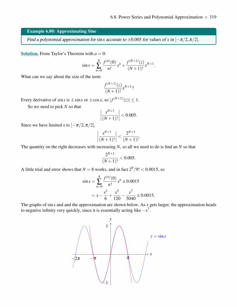
6.8. Power Series and Polynomial Approximation 319
Example 6.80: Approximating Sine
Find a polynomial approximation for sinx accurate to ±0.005 for values of x in [−π/2,π/2].
Solution. From Taylor’s Theorem with a = 0:
sinx =N
∑n=0
f (n)(0)
n!xn +
f (N+1)(z)
(N +1)!xN+1.
What can we say about the size of the term
f (N+1)(z)
(N +1)!xN+1?
Every derivative of sinx is ±sinx or ±cosx, so | f (N+1)(z)| ≤ 1.
So we need to pick N so that∣
∣
∣
∣
xN+1
(N +1)!
∣
∣
∣
∣
< 0.005.
Since we have limited x to [−π/2,π/2],∣
∣
∣
∣
xN+1
(N +1)!
∣
∣
∣
∣
<2N+1
(N+1)!.
The quantity on the right decreases with increasing N, so all we need to do is find an N so that
2N+1
(N +1)!< 0.005.
A little trial and error shows that N = 8 works, and in fact 29/9! < 0.0015, so
sinx =8
∑n=0
f (n)(0)
n!xn ±0.0015
= x− x3
6+
x5
120− x7
5040±0.0015.
The graphs of sinx and and the approximation are shown below. As x gets larger, the approximation heads
to negative infinity very quickly, since it is essentially acting like −x7.
y = sinx
−2π −π π
−1
1
x
y
320 Sequences and Series
♣
Note: We can now approximate the value of sin(x) to within 0.005 by using simple trigonometric identities
to translate x into the interval [−π/2,π/2].
We can extract a bit more information from this example.
Example 6.81: Convergence of Power Series Representation of Sine
Show that
sinx =∞
∑n=0
f (n)(0)
n!xn
by showing that limn→∞
Rn(x) = 0.
Solution. If we do not limit the value of x, we still have∣
∣
∣
∣
∣
f (N+1)(z)
(N +1)!xN+1
∣
∣
∣
∣
∣
≤∣
∣
∣
∣
xN+1
(N +1)!
∣
∣
∣
∣
so that sinx is represented byN
∑n=0
f (n)(0)
n!xn ±
∣
∣
∣
∣
xN+1
(N +1)!
∣
∣
∣
∣
.
If we can show that
limN→∞
∣
∣
∣
∣
xN+1
(N +1)!
∣
∣
∣
∣
= 0
for each x then
sinx =∞
∑n=0
f (n)(0)
n!xn =
∞
∑n=0
(−1)n x2n+1
(2n+1)!,
that is, the sine function is actually equal to its Maclaurin series for all x. How can we prove that the
limit is zero? Suppose that N is larger than |x|, and let M be the largest integer less than |x| (if M = 0 the
following is even easier). Then
|xN+1|(N +1)!
=|x|
N +1
|x|N
|x|N −1
· · · |x|M+1
|x|M
|x|M−1
· · · |x|2
|x|1
≤ |x|N +1
·1 ·1 · · ·1 · |x|M
|x|M−1
· · · |x|2
|x|1
=|x|
N +1
|x|MM!
.
The quantity |x|M/M! is a constant, so
limN→∞
|x|N +1
|x|MM!
= 0
and by the Squeeze Theorem 6.7
limN→∞
∣
∣
∣
∣
xN+1
(N +1)!
∣
∣
∣
∣
= 0
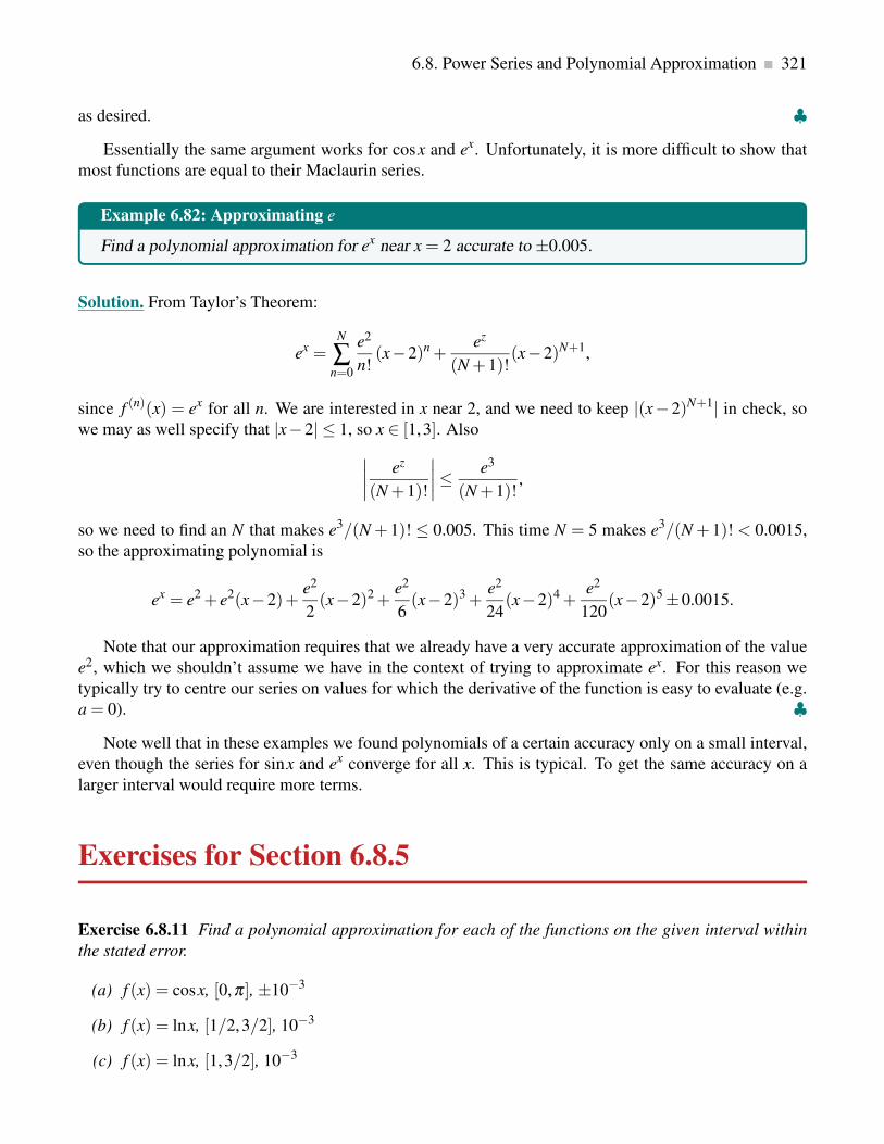
6.8. Power Series and Polynomial Approximation 321
as desired. ♣
Essentially the same argument works for cosx and ex. Unfortunately, it is more difficult to show that
most functions are equal to their Maclaurin series.
Example 6.82: Approximating e
Find a polynomial approximation for ex near x = 2 accurate to ±0.005.
Solution. From Taylor’s Theorem:
ex =N
∑n=0
e2
n!(x−2)n +
ez
(N +1)!(x−2)N+1,
since f (n)(x) = ex for all n. We are interested in x near 2, and we need to keep |(x−2)N+1| in check, so
we may as well specify that |x−2| ≤ 1, so x ∈ [1,3]. Also
∣
∣
∣
∣
ez
(N +1)!
∣
∣
∣
∣
≤ e3
(N+1)!,
so we need to find an N that makes e3/(N +1)! ≤ 0.005. This time N = 5 makes e3/(N +1)! < 0.0015,
so the approximating polynomial is
ex = e2 + e2(x−2)+e2
2(x−2)2 +
e2
6(x−2)3 +
e2
24(x−2)4 +
e2
120(x−2)5 ±0.0015.
Note that our approximation requires that we already have a very accurate approximation of the value
e2, which we shouldn’t assume we have in the context of trying to approximate ex. For this reason we
typically try to centre our series on values for which the derivative of the function is easy to evaluate (e.g.
a = 0). ♣
Note well that in these examples we found polynomials of a certain accuracy only on a small interval,
even though the series for sinx and ex converge for all x. This is typical. To get the same accuracy on a
larger interval would require more terms.
Exercises for Section 6.8.5
Exercise 6.8.11 Find a polynomial approximation for each of the functions on the given interval within
the stated error.
(a) f (x) = cosx, [0,π ], ±10−3
(b) f (x) = lnx, [1/2,3/2], 10−3
(c) f (x) = lnx, [1,3/2], 10−3

322 Sequences and Series
Exercise 6.8.12 Show that each function is equal to its Taylor series for all x by showing that limn→∞
Rn(x) =
0.
(a) f (x) = cosx
(b) f (x) = ex

Selected Exercise Answers
1.2.1 10
1.2.2 35/3
1.3.1 x2
1.3.2 2x2
1.3.3 2x2 −8
1.3.4 2b2 −2a2
1.3.5 4 rectangles: 41/4 = 10.25, 8 rectangles: 183/16 = 11.4375
1.3.6 23/4
1.4.1 (a) 8
(b) 2
(c) 9.3339
(d) 2
1.4.2 (a) 87/2
(b) 2
(c) ln(10)
(d) e5 −1
(e) 34/4
(f) 26/6−1/6
(g) 16√
2−2
(h)2
3
(i)2√
2
3
(j)log14− log5
3
(k) −1
1.4.3 (a) x2 −3x
(b) 2x(x4 −3x2)
(c) ex2
(d) 2xex4
(e) tan(x2)
(f) 2x tan(x4)−10tan(100x2)
323

324 Selected Exercise Answers
1.4.4 31, 14
1.4.5 5
1.4.7 (a) $530.40
(b) $119.60
1.4.8 (a) $7500
(b) $2500
1.5.1 (a) (16/3)x3/2 +C
(b) t3+ t +C
(c) 8√
y+C
(d) −2/z+C
(e) 7 lns+C
(f) (5x+1)3/15+C
(g) (t −6)3/3+C
(h) 2z5/2/5+C
(i) −4/√
x+C
(j) 4t − t2 +C, t < 2; t2 −4t +8+C, t ≥ 2
(k) (sinx−4) · cosx+C
(l) y2 − tany+C
(m) cotx+ secx+C
1.5.2 (a)s
6
(
4s2 +3s−6)
+C
(b) s3 −0.5s2 + s−2logs+C
(c)u8/3 −3
3√
2
4u2/3+C
(d)8√
t + t logt −4
4t+C
1.5.3 (a) f (t) = 32t2+2t +5
(b) f (t) = t +3logt −2
(c) f (t) =−cos t −1
(d) f (t) = 0.5e2t −4t
1.5.4 (a) R(q) = 16q−0.004q2
(b) p(q) = 16q−0.004q2
q
1.5.5 $36,400 when q = 5000 heads.
1.5.6 C(q) = 0.0005q2+50q+500
1.5.7 (a) N(t) = −23 t3 +5t2+100t +1 for 0 ≤ t ≤ 5.
(b) 272
2.1.1

Selected Exercise Answers 325
−(1− t)10/10+C
(a)(b) x5/5+2x3/3+ x+C
(c) (x2 +1)101/202+C
(d) −3(1−5t)2/3/10+C
(e) (sin4 x)/4+C
(f) −(100− x2)3/2/3+C
(g) −2√
1− x3/3+C
(h) sin(sinπt)/π +C
(i) 1/(2cos2 x) = (1/2)sec2 x+C
(j) − ln |cosx|+C
(k) tan2(x)/2+C
(l) −cos(tanx)+C
(m) (27/8)(x2 −7)8/9
(n) f (x)2/2
2.1.2 (a) 0
(b) 1/4
(c) 1/10
(d)√
3/4
(e) −(37 +1)/14
(f) 0
2.1.3 15e−0.2t +9985 trucks.
2.1.4 p(q) = 100(1/(1−q)+ log(q−1))+102
2.1.5 p(q) = 200√q2+3
−97
2.1.2 Approximately 300 units.
2.2.1 (a) x/2− sin(2x)/4+C
(b) −cosx+(cos3 x)/3+C
(c) 3x/8− (sin2x)/4+(sin4x)/32+C
(d) (cos5 x)/5− (cos3 x)/3+C
(e) sinx− (sin3 x)/3+C
(f) (sin3 x)/3− (sin5 x)/5+C
(g) −2(cosx)5/2/5+C
(h) tanx− cotx+C
(i) (sec3 x)/3− secx+C
(j) −cosx+ sinx+C
(k)3
2ln |secx+ tanx|+ tanx+
1
2secx tanx+C
(l)tan5(x2)
10+C
(m)tan5(x2)
10+C
2.3.1 (a) x√
x2 −1/2− ln |x+√
x2 −1|/2+C
(b) x√
9+4x2/2+(9/4) ln |2x+√
9+4x2|+C
(c) −(1− x2)3/2/3+C
(d) arcsin(x)/8− sin(4arcsinx)/32+C
(e) ln |x+√
1+ x2|+C
(f) (x+1)√
x2 +2x/2−ln |x+1+√
x2 +2x|/2+C
(g) −arctanx−1/x+C
(h) 2arcsin(x/2)− x√
4− x2/2+C
(i) arcsin(√
x)−√
x√
1− x+C
(j) (2x2 +1)√
4x2 −1/24+C

326 Selected Exercise Answers
2.4.1 (a) (1/2)ex2+C
(b) (x/2)− sin(2x)/4+C =(x/2)− (sinxcosx)/2+C
(c) (x2 arctanx+ arctanx− x)/2+C
(d) x2/4− (cos2 x)/4− (xsinxcosx)/2+C
(e) x/4− (xcos2 x)/2+(cosxsinx)/4+C
2.4.2 (a) cosx+ xsinx+C
(b) x2 sinx−2sinx+2xcosx+C
(c) (x−1)ex +C
(d) x lnx− x+C
(e) −x3 cosx+3x2 sinx+6xcosx−6sinx+C
(f) x3 sinx+3x2 cosx−6xsinx−6cosx+C
(g) xarctan(√
x)+ arctan(√
x)−√x+C
(h) 2sin(√
x)−2√
xcos(√
x)+C
(i) secxcscx−2cotx+C
2.5.1 (a) − ln |x−2|/4+ ln |x+2|/4+C
(b) −x3/3−4x−4ln |x−2|+4ln |x+2|+C
(c) −1/(x+5)+C
(d) −x− ln |x−2|+ ln |x+2|+C
(e) −4x+ x3/3+8arctan(x/2)+C
(f) (1/2)arctan(x/2+5/2)+C
(g) x2/2−2ln(4+ x2)+C
(h) (1/4) ln |x+3|− (1/4) ln |x+7|+C
(i) (1/5) ln |2x−3|− (1/5) ln |1+ x|+C
(j) (1/3) ln |x|− (1/3) ln |x+3|+C
2.6.1 (a) T,S: 4±0
(b) T: 9.28125±0.281125; S: 9±0
(c) T: 60.75±1; S: 60±0
(d) T: 1.1167±0.0833; S: 1.1000±0.0167
(e) T: 0.3235±0.0026; S: 0.3217±0.000065
(f) T: 0.6478±0.0052; S: 0.6438±0.000033
(g) T: 2.8833±0.0834; S: 2.9000±0.0167
(h) T: 1.1170±0.0077; S: 1.1114±0.0002
(i) T: 1.097±0.0147; S: 1.089±0.0003
(j) T: 3.63±0.087; S: 3.62±0.032
2.7.1 (a) Converges to π/2
(b) Divergent (to ∞)
(c) Converges to 1
(d) Divergent (to ∞)
(e) Converges to 53(4
3/5)
(f) Converges to 1
(g) Divergent
(h) Converges to 1/3
(i) Divergent
(j) Converges to π2
2+2π2
(k) Converges to π
(l) Divergent

Selected Exercise Answers 327
2.7.3 0 < p < 1
2.8.1(t +4)4
4+C
2.8.2(t2−9)5/2
5+C
2.8.3(et2
+16)2
4+C
2.8.4 cos t − 2
3cos3 t +C
2.8.5tan2 t
2+C
2.8.6 ln |t2+ t +3|+C
2.8.71
8ln |1−4/t2|+C
2.8.81
25tan(arcsin(t/5))+C =
t
25√
25− t2+C
2.8.92
3
√sin3t +C
2.8.10 t tant + ln |cos t|+C
2.8.11 2√
et +1+C
2.8.123t
8+
sin2t
4+
sin4t
32+C
2.8.13ln |t|
3− ln |t +3|
3+C
2.8.14−1
sinarctan t+C =−
√
1+ t2/t +C
2.8.15−1
2(1+ tant)2+C
2.8.16(t2+1)5/2
5− (t2+1)3/2
3+C

328 Selected Exercise Answers
2.8.17et sint − et cos t
2+C
2.8.18(t3/2+47)4
6+C
2.8.192
3(2− t2)3/2− 1
(2− t2)1/2+C
2.8.20ln |sin(arctan(2t/3))|
9+C = (ln(4t2)− ln(9+4t2))/18+C
2.8.21(arctan(2t))2
4+C
2.8.223ln |t +3|
4+
ln |t −1|4
+C
2.8.23cos7 t
7− cos5 t
5+C
2.8.24−1
t −3+C
2.8.25−1
lnt+C
2.8.26t2(lnt)2
2− t2 ln t
2+
t2
4+C
2.8.27 (t3−3t2+6t −6)et +C
2.8.285+
√5
10ln(2t +1−
√5)+
5−√
5
10ln(2t +1+
√5)+C
3.1.1 (a) 2/π; 2/π; 0
(b) 4/3
(c) 1/a
(d) π/4
3.1.2 (a) 8√
2/15
(b) 2/3−2/π
(c) 3/π −3√
3/(2π)−1/8

Selected Exercise Answers 329
(d) 1/3
(e) 1/5
(f) 1/6
3.1.3 (a) 1/12
(b) 500/3
3.1.4 (a) 9/2
(b) 4/3
(c) 10√
5/3−6
(d) 2
3.1.5 (a) 6.75
(b) 12.15
(c) 16/3
(d) 3 log(2)
(e) 4.5
(f) 1/3
3.1.6 It rises until t = 100/49, then falls. The position of the object at time t is s(t) = −4.9t2 +20t + k.
The net distance travelled is −45/2, that is, it ends up 45/2 meters below where it started. The total
distance travelled is 6205/98 meters.
3.1.7
∫ 2π
0sint dt = 0
3.1.8 net: 2π , total: 2π/3+4√
3
3.1.9 8
3.1.10 17/3
3.1.11 A = 18, B = 44/3, C = 10/3
3.3.1 (a) (1/3)(area of base)(height)
(b) 2π
3.3.2 (a) 4π/3

330 Selected Exercise Answers
(b) 50π/3
(c) π/2
(d) π/4
3.3.3 (a) 26π/5
(b) π/7
(c) 16π/3
(d) π
(e) 1.5420
(f) 8π/3
(g) 8π/3
(h) π(π/2−1)
3.3.4 (a) 2π/4
(b) 256√
2π/13
(c) π
(d) π/2
3.3.6 (a) 16π/3
(b) 9π/2
(c) 117π/5
(d) 625π/3
3.3.7 16π , 24π
3.3.9 πh2(3r−h)/3
3.4.5 (a) 114π/5
(b) 74π/5
(c) 20π
(d) 4π
4.1.1 (a) z = y2, z = x2, z = 0, lines of slope 1
(b) z = |y|, z = |x|, z = 2|x|, diamonds
(c) z = e−y2sin(y2), z = e−x2
sin(x2), z = e−2x2sin(2x2), circles

Selected Exercise Answers 331
(d) z =−sin(y), z = sin(x), z = 0, lines of slope 1
(e) z = y4, z = x4, z = 0, hyperbolas
4.1.2 (a) {(x,y) | |x| ≤ 3 and |y| ≥ 2}
(b) {(u,v) | u2 + v2 ≤ 2}
(c) {(x,y) | x2 +4y2 ≤ 16}
(d) All real x and y.
(e) All real x,y, and z
(f) {(x,y) | 1 ≤ x2 + y2 ≤ 3}
(g) {(u,v) | u 6= v}
(h) All real s and t
(i) {(r,s) | rs > 0}
(j) All real x and y
(k) {(x,y) | x+ y > 7}
4.1.4

332 Selected Exercise Answers
We draw the level curves of f :
(a)
−2 2
−1
1
x
y
(b)
−3 3
4
x
y
(c)
−2 2
1x
y
(d)
1
1x
y
(e)
4 5
x
y
(f)
1
1x
y
4.1.5 (a) R(qc,qb) =1
420
(
−105q2c −102qcqb +42000qc−140q2
b +63000qb
)
(b) The region where all of pc, pb,qc,qb ≥ 0.
4.1.6 (a) R(x,y) =−0.1q2b −0.9qbqc +10qb −q2
c +30qc
(b) The region where all of pb, pc,qb,qc ≥ 0.
4.1.7 $50,148.53; $28,661.05

Selected Exercise Answers 333
4.1.8 About 39 tires.
4.2.1 (a) 16
(b) 4
(c) 15/8
(d) 1/2
(e) 5/6
(f) 12−65/(2e)
(g) 1/2
(h) π/64
(i) (2/9)23/2 − (2/9)
(j) (1− cos(1))/4
(k) (2√
2−1)/6
(l) π −2
(m) (e9 −1)/6
(n)4
15− π
4
(o) 1/3
4.2.2 (a) 4/5
(b) 8π
(c) 2
(d) 5/3
(e) 81/2
(f) 2a3/3
(g) 4π
(h) π/32
(i) 31/8
(j) 128/15
4.2.3 448
4.2.4 1800π m3
4.2.5(e2 +8e+16)
15
√e+4− 5
√5
3− e5/2
15+
1
15
4.3.1 (a) 11/24
(b) 623/60
(c) −3e2/4+2e−3/4
(d) 1/20
(e) π/48
(f) 11/84
(g) 151/60
(h) π
4.3.23π
16
4.4.2 (a) f (x) = 29(3− x), x ∈ [0,3]
(b) f (x) = 4x5 , x ∈ [1,∞)
(c) f (x,y) = 6xy2, (x,y) ∈ [0,1]× [0,1]
(d) f (x,y) = 3e7 x2e−y, (x,y) ∈ [1,2]× [1,∞)
4.4.3 (a) i.0, ii. 0.173, iii.≈ 1, iv. 0.0498
(b) i. 0.739, ii. 0.261, iii.0.599, iv. 0.739
(c) i. 0.25, ii. 0

334 Selected Exercise Answers
(d) i. 0.0469, ii. 0.109
4.4.5 No; f (−1)< 0
4.4.6 (a) 0.318
(b) 0.0067
4.4.7 (c) i.3, ii.3, iii.√
3
4.4.8 (a) 0.2
(b) 0.5
4.4.9 2 minutes
4.4.10 5 kg
4.4.11 (a) Not independent
4.4.12 (a) i.3/4,4/7; ii.3/80,19/392; iii.1/63
5.1.1 (a) third order, non-linear
(b) third order, linear
(c) first order, non-linear
(d) fourth order, non-linear
(e) second order, linear
(f) first order, non-linear
5.1.2 (a) non-homogeneous
(b) homogeneous
(c) non-homogeneous
(d) homogeneous
(e) non-homogeneous
(f) homogeneous
5.1.3 (a) has constant coefficients
(b) does not have constant coefficients

Selected Exercise Answers 335
(c) does not have constant coefficients
(d) does not have constant coefficients
(e) does not have constant coefficients
(f) does not have constant coefficients
5.2.2 (a) y = nπ , for any integer n.
(b) none
5.2.3 (a) y = arctan t +C
(b) y = t lnt − t +C
(c) y =±√
t2+C
(d) y =±1, y = (1+Ae2t)/(1−Ae2t)
(e) y4/4−5y = t2/2+C
(f) y = M+Ae−kt
5.2.4 (a) y =tn+1
n+1+1
(b) y = (2t/3)3/2 and y(t) = 0
(c) y = 2e3t/2
5.2.510ln(15/2)
ln5≈ 2.52 minutes
5.2.6 t =− ln2
k
5.2.7 600e−6ln2/5 ≈ 261 mg;5 ln300
ln2≈ 41 days
5.2.8 100e−200ln2/191 ≈ 48 mg;5730ln50
ln2≈ 32339 years
5.2.9 y = y0et ln2
5.2.10 500e−5ln2/4 ≈ 210 g
5.2.11 y =M
1+Ae−Mkt

336 Selected Exercise Answers
5.3.1 (a) y = Ae−5t
(b) y = Ae2t
(c) y = Ae−arctan t
(d) y = Ae−t3/3
5.3.2 (a) y = 4e−t
(b) y =−2e3t−3
(c) y = e1+cos t
(d) y = e2e−et
(e) y = 0
(f) y = 0
(g) y = 4t2
(h) y =−2e(1/t)−1
(i) y = e1−t−2
(j) y = 0
5.3.3 (a) y = Ae−4t +2
(b) y = Ae2t −3
(c) y = Ae−(1/2)t2+5
(d) y = Ae−et −2
(e) y = Aet − t2−2t −2
(f) y = Ae−t/2 + t −2
5.3.4 (a) y = At2− 1
3t
(b) y =c
t+
2
3
√t
(c) y = Acos t + sin t
(d) y =A
sec t + tan t+1− t
sec t + tan t
5.3.5 (a) y = 2− e−4t

Selected Exercise Answers 337
(b) y = 6e2t −3
(c) y = 5−4e2−(1/2)t2
(d) y = e−et −2
(e) y = 6et − t2−2t −2
(f) y = t −2
5.3.6 k = ln5, y = 100e−t ln5
5.3.7 k =−12/13, y = exp(−13t1/13)
5.3.8 y = 106et ln(3/2)
5.3.9 y = 10e−t ln(2)/6
5.4.1 (a) B
(b) A
(c) C
(d) D
5.4.4 (a) y(1)≈ 1.355
(b) y(1)≈ 40.31
(c) y(1)≈ 1.05
(d) y(1)≈ 2.30
6.1.2 1
6.1.4 (a) diverges
(b) converges to 1
(c) diverges
(d) converges to 0
(e) converges to 0
(f) converges to 1
(g) converges to 1
(h) converges to 0

338 Selected Exercise Answers
6.2.1 (a) limn→∞
n2/(2n2 +1) = 1/2
(b) limn→∞
5/(21/n +14) = 1/3
(c)∞
∑n=1
1
ndiverges, so
∞
∑n=1
31
ndiverges
6.2.2 (a) −3/2
(b) 11
(c) 20
(d) 3/4
(e) 3/2
(f) 3/10
6.3.1 (a) diverges
(b) diverges
(c) converges
(d) converges
(e) converges
(f) converges
(g) diverges
(h) converges
6.3.2 (a) N = 5
(b) N = 10
(c) N = 1687
(d) any integer greater than e200
6.4.1 (a) converges
(b) converges
(c) diverges
(d) converges

Selected Exercise Answers 339
6.4.2 (a) 0.90
(b) 0.95
6.5.1 (a) converges
(b) converges
(c) converges
(d) diverges
(e) diverges
(f) diverges
(g) converges
(h) diverges
(i) converges
(j) diverges
6.6.1 (a) converges absolutely
(b) diverges
(c) converges conditionally
(d) converges absolutely
(e) converges conditionally
(f) converges absolutely
(g) diverges
(h) converges conditionally
6.7.2 (a) converges
(b) converges
(c) converges
(d) diverges
6.8.1 (a) R = 1, I = (−1,1)
(b) R = ∞, I = (−∞,∞)
(c) R = e, I = (2− e,2+ e)

340 Selected Exercise Answers
(d) R = 0, converges only when x = 2
(e) R = 1, I = [−6,−4]
(f) R = e
6.8.2 (a) the alternating harmonic series
6.8.3 (a)∞
∑n=0
(n+1)xn
(b)∞
∑n=0
(n+1)(n+2)xn
(c)∞
∑n=0
(n+1)(n+2)
2xn, R = 1
(d) C+∞
∑n=0
−1
(n+1)(n+2)xn+2
6.8.4 (a)∞
∑n=0
(−1)nx2n/(2n)!, R = ∞
(b)∞
∑n=0
xn/n!, R = ∞
6.8.5 (a)∞
∑n=0
(−1)n (x−5)n
5n+1, R = 5
(b)∞
∑n=1
(−1)n−1 (x−1)n
n, R = 1
(c) ln(2)+∞
∑n=1
(−1)n−1 (x−2)n
n2n, R = 2
(d)∞
∑n=0
(−1)n(n+1)(x−1)n, R = 1
6.8.6 (a) 1+∞
∑n=1
1 ·3 ·5 · · ·(2n−1)
n!2nxn = 1+
∞
∑n=1
(2n−1)!
22n−1(n−1)!n!xn, R = 1
6.8.7 T5(x) = x− x3
3! +x5
5!
(a) sin(0.1)≈ T5(0.1)≈ 0.10016675
(b) sin(0.1)= 0.0998334 . . . using a calculator. Our approximation is accurate to 0.10016675−0.0998334 . . .=0.0003̄.

Selected Exercise Answers 341
6.8.8 T3(x) = x+ x2 + x3. The point x = 5 is not close to x = 0, and f is not continuous at x = 1.
6.8.9 (a) f (n)(x) =(−1)(n−1)(n−1)!
xn
(b) Tn(x) = ln(1)+n
∑i=1
( (−1)(i−1)(i−1)!1n
)
i!(x− 1)i =
n
∑i=1
(
(−1)(i−1)(i−1)!
i!
)
(x− 1)i since ln(1) = 0 and
1n = 1.
6.8.10 0.262364...
6.8.11 (a) 1− x2
2+
x4
24− x6
720+ · · ·+ x12
12!

Index
absolute convergence test, 293
alternating harmonic series, 288
antiderivative, 3
general antiderivative, 38
antidifferentiation, 3
area, 24, 25
area between two curves, 114, 119
net area, 24, 25
average value, 109, 180
bell curve, 209
comparison test, 291
for improper integrals, 104
for series, 291
continuous money flow, 128
future value, 132, 133
present value, 131
total income, 129
present value, 130
contour map, 173
convergence, 276
absolutely, 294
conditionally, 294
covariance, 220
cumulative distribution, 198
bell-shaped, 209
exponential, 199, 200
joint, 214
normal, 199, 209
standard normal, 202, 209
uniform, 199
cylindrical shell, 154
definite integral, 24, 39
geometric interpretation, 25
lower limit of integration, 24
properties, 26
upper limit of integration, 24
derivative, 3
differential equation, 44, 225
Euler’s method, 257
first order, 229
standard form, 244
general solution, 234, 244
initial conditions, 231
initial value problem, 45, 231, 242, 245, 247
integrating factor, 246, 247
linear, 226, 243
constant coefficients, 227
homogeneous, 227, 242
non-homogeneous, 227, 243
long-term behaviour, 251
non-linear, 226
numerical methods, 257
order, 226
particular solution, 234
separable, 233
separation of variables, 233, 234
slope field, 250
solution, 225
variation of parameters, 244, 245
discrete probability, 194
disk, 141
disk method, 148
divergence, 276
double integral, 180
dummy variable, 24
Euler’s method, 257, 259
non-uniform, 259
uniform, 259
expected value, 195, 202, 203, 217
average, 202
mean, 202
first order differential equation, 229
first order homogeneous linear equation, 242
first order linear differential equation, 243
Fubini’s Theorem, 183, 186
function
continuous, 95
multi-variable, 168
single-variable, 168
fundamental theorem of calculus, 27, 95
342

INDEX 343
and chain rule, 35
geometric sequence, 272
common ratio, 272
growth and decay
carrying capacity, 238
growth rate constant, 236–238
logistic, 238, 240
simple, 236, 237
harmonic series, 281
improper integral, 96, 98
comparison test, 104
converges, 97
diverges, 97
improper integrals
p-integrals, 102
p-test, 103
indefinite integral, 39
index, 11
initial value problem, 231
integrable, 24
integral sign, 24, 39
integral test, 284
integrand, 24, 39
integrating, 24, 39
integrating factor, 246
integration, 3, 24, 39
area, 6
by parts, 75
definite
Riemann sums, 22
displacement, 4
partial fractions, 80, 87
products of secant and tangent, 65
products of sine and cosine, 59
rules, 41
substitution rule, 48, 56
trapezoid approximation, 89
trigonometric substitution, 70
integration by parts, 75
tabular method, 78
interval of convergence, 301
joint cumulative distribution function, 214
joint probability density function, 212
left hand rule, 8, 14
level curve, 173
level set, 175
level surface, 175
Maclaurin series, 308
midpoint rule, 8, 14, 89
error bound, 89
multi-variable, 168
normal distribution, 209
characteristics, 209
p-series, 284
partial fraction decomposition, 84
power series, 299, 300
centred at a, 302
convergence, 302
derivative, 305
integral, 305
interval of convergence, 301
radius of convergence, 301
probability, 199, 216
independent, 215
probability density function, 196
joint, 212
marginal, 212
uniform, 199
quadratic formula, 81
radius of convergence, 301
random variable, 195
continuous, 196
discrete, 196
random variables
independent, 212, 215
ratio test, 297
rational function, 80
Riemann sum, 7, 16, 22
right hand rule, 8, 14
root test, 298
sequence, 266
bounded, 273
bounded above, 273
bounded below, 273
boundedness, 272

344 INDEX
converves, 267
decreasing, 272
diverges, 267
geometric, 271
increasing, 272
limit, 267
monotonic, 272
monotonicity, 272
n-th term, 266
non-decreasing, 272
non-increasing, 272
properties, 269
strictly decreasing, 272
strictly increasing, 272
term, 266
series, 266, 275, 276
absolute convergence test, 293
alternating harmonic, 287, 288
comparison test, 291
converges, 276
diverges, 276
geometric, 276
harmonic, 279–281
Maclaurin, 308
p-series, 284
ratio test, 297
root test, 298
sequence of partial sums, 276
Taylor, 309, 310
shell method, 154, 158
sigma notation, 10, 11
Simpson’s rule, 93, 94
error bound, 94
single-variable, 168
slope field, 250
family of curves, 256
standard deviation, 205, 206, 218
standard normal distribution, 209
characteristics, 210
substitution
inverse substitution, 69
trigonometric substitution, 69
substitution rule
guideline for substitution rule, 49
summation
formulas, 12
notation, 10
properties, 12
summation symbol, 11
surplus, 123
consumer surplus, 125
producer surplus, 126
Taylor polynomial, 313
Taylor series, 309, 310
Taylor’s theorem, 316, 317
remainder, 318
trapezoid rule, 89–91
error bound, 91
trigonometric substitution, 69
guideline for trigonometric substitution, 70
triple integral, 188
variable of integration, 24, 39
variance, 205, 206, 218
variation of parameters, 244
volume, 136
axis of rotation, 140
cross-section, 136
cylindrical shell, 154
disk, 141
disk method, 148
shell method, 154, 158
solid of revolution, 140
washer method, 144, 150
volume below a surface, 180
washer method, 144, 150