CalculiXUSER’SMANUAL -CalculiXGraphiX,Version2.14- ·...
159
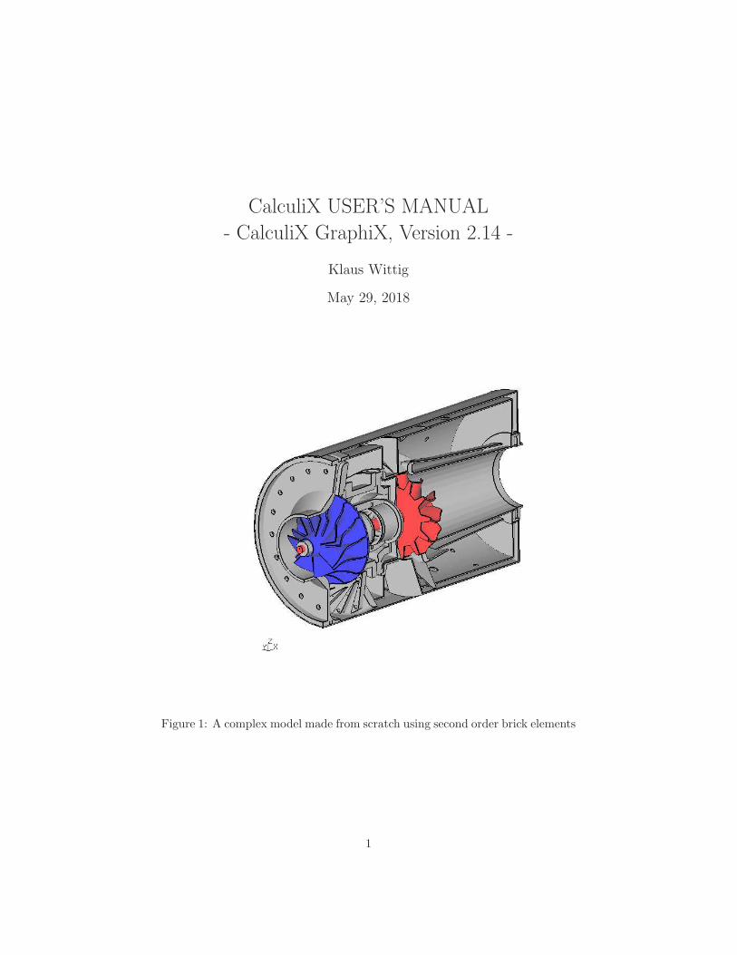
CalculiX USER’S MANUAL - CalculiX GraphiX, Version 2.14 - Klaus Wittig May 29, 2018 Figure 1: A complex model made from scratch using second order brick elements 1
-
Upload
phungthuan -
Category
Documents
-
view
227 -
download
0
Transcript of CalculiXUSER’SMANUAL -CalculiXGraphiX,Version2.14- ·...
CalculiX USER’S MANUAL
- CalculiX GraphiX, Version 2.14 -
Klaus Wittig
May 29, 2018
Figure 1: A complex model made from scratch using second order brick elements
1
Contents
1 Introduction 7
2 Concept 8
3 File Formats 9
4 Getting Started 10
5 Program Parameters 14
6 Input Devices 156.1 Mouse . . . . . . . . . . . . . . . . . . . . . . . . . . . . . . . . . 156.2 Keyboard . . . . . . . . . . . . . . . . . . . . . . . . . . . . . . . 16
7 Menu 177.1 Datasets . . . . . . . . . . . . . . . . . . . . . . . . . . . . . . . . 18
7.1.1 Entity . . . . . . . . . . . . . . . . . . . . . . . . . . . . . 187.2 Viewing . . . . . . . . . . . . . . . . . . . . . . . . . . . . . . . . 18
7.2.1 Show Elements With Light . . . . . . . . . . . . . . . . . 187.2.2 Show Bad Elements . . . . . . . . . . . . . . . . . . . . . 187.2.3 Fill . . . . . . . . . . . . . . . . . . . . . . . . . . . . . . . 187.2.4 Lines . . . . . . . . . . . . . . . . . . . . . . . . . . . . . . 197.2.5 Dots . . . . . . . . . . . . . . . . . . . . . . . . . . . . . . 197.2.6 Toggle Culling Back/Front . . . . . . . . . . . . . . . . . 197.2.7 Toggle Illuminate Backface . . . . . . . . . . . . . . . . . 197.2.8 Toggle Model Edges . . . . . . . . . . . . . . . . . . . . . 197.2.9 Toggle Element Edges . . . . . . . . . . . . . . . . . . . . 197.2.10 Toggle Surfaces/Volumes . . . . . . . . . . . . . . . . . . 197.2.11 Toggle Move-Z/Zoom . . . . . . . . . . . . . . . . . . . . 207.2.12 Toggle Background Color . . . . . . . . . . . . . . . . . . 207.2.13 Toggle Vector-Plot . . . . . . . . . . . . . . . . . . . . . . 207.2.14 Toggle Add-Displacement . . . . . . . . . . . . . . . . . . 207.2.15 Toggle Shaded Result . . . . . . . . . . . . . . . . . . . . 20
7.3 Animate . . . . . . . . . . . . . . . . . . . . . . . . . . . . . . . . 217.3.1 Start . . . . . . . . . . . . . . . . . . . . . . . . . . . . . . 217.3.2 Tune-Value . . . . . . . . . . . . . . . . . . . . . . . . . . 217.3.3 Steps per Period . . . . . . . . . . . . . . . . . . . . . . . 217.3.4 Time per Period . . . . . . . . . . . . . . . . . . . . . . . 217.3.5 Toggle Real Displacements . . . . . . . . . . . . . . . . . 217.3.6 Toggle Static Model Edges . . . . . . . . . . . . . . . . . 217.3.7 Toggle Static Element Edges . . . . . . . . . . . . . . . . 217.3.8 Toggle Dataset Sequence . . . . . . . . . . . . . . . . . . . 22
7.4 Frame . . . . . . . . . . . . . . . . . . . . . . . . . . . . . . . . . 227.5 Zoom . . . . . . . . . . . . . . . . . . . . . . . . . . . . . . . . . 227.6 Center . . . . . . . . . . . . . . . . . . . . . . . . . . . . . . . . . 22
2
7.7 Enquire . . . . . . . . . . . . . . . . . . . . . . . . . . . . . . . . 227.8 Cut . . . . . . . . . . . . . . . . . . . . . . . . . . . . . . . . . . 227.9 Graph . . . . . . . . . . . . . . . . . . . . . . . . . . . . . . . . . 237.10 User . . . . . . . . . . . . . . . . . . . . . . . . . . . . . . . . . . 237.11 Orientation . . . . . . . . . . . . . . . . . . . . . . . . . . . . . . 23
7.11.1 +x View . . . . . . . . . . . . . . . . . . . . . . . . . . . . 237.11.2 -x View . . . . . . . . . . . . . . . . . . . . . . . . . . . . 237.11.3 +y View . . . . . . . . . . . . . . . . . . . . . . . . . . . . 237.11.4 -y View . . . . . . . . . . . . . . . . . . . . . . . . . . . . 237.11.5 +z View . . . . . . . . . . . . . . . . . . . . . . . . . . . . 237.11.6 -z View . . . . . . . . . . . . . . . . . . . . . . . . . . . . 23
7.12 Hardcopy . . . . . . . . . . . . . . . . . . . . . . . . . . . . . . . 237.12.1 Tga-Hardcopy . . . . . . . . . . . . . . . . . . . . . . . . 247.12.2 Ps-Hardcopy . . . . . . . . . . . . . . . . . . . . . . . . . 247.12.3 Gif-Hardcopy . . . . . . . . . . . . . . . . . . . . . . . . . 247.12.4 Png-Hardcopy . . . . . . . . . . . . . . . . . . . . . . . . 247.12.5 Start Recording Gif-Movie . . . . . . . . . . . . . . . . . . 24
7.13 Help . . . . . . . . . . . . . . . . . . . . . . . . . . . . . . . . . . 247.14 Quit . . . . . . . . . . . . . . . . . . . . . . . . . . . . . . . . . . 24
8 Customization 25
9 Commands 259.1 anim . . . . . . . . . . . . . . . . . . . . . . . . . . . . . . . . . . 269.2 area . . . . . . . . . . . . . . . . . . . . . . . . . . . . . . . . . . 269.3 asgn . . . . . . . . . . . . . . . . . . . . . . . . . . . . . . . . . . 279.4 bia . . . . . . . . . . . . . . . . . . . . . . . . . . . . . . . . . . . 279.5 body . . . . . . . . . . . . . . . . . . . . . . . . . . . . . . . . . . 289.6 break . . . . . . . . . . . . . . . . . . . . . . . . . . . . . . . . . . 299.7 call . . . . . . . . . . . . . . . . . . . . . . . . . . . . . . . . . . . 299.8 cntr . . . . . . . . . . . . . . . . . . . . . . . . . . . . . . . . . . 299.9 comp . . . . . . . . . . . . . . . . . . . . . . . . . . . . . . . . . . 299.10 copy . . . . . . . . . . . . . . . . . . . . . . . . . . . . . . . . . . 309.11 corrad . . . . . . . . . . . . . . . . . . . . . . . . . . . . . . . . . 329.12 csysa . . . . . . . . . . . . . . . . . . . . . . . . . . . . . . . . . . 329.13 cut . . . . . . . . . . . . . . . . . . . . . . . . . . . . . . . . . . . 339.14 del . . . . . . . . . . . . . . . . . . . . . . . . . . . . . . . . . . . 339.15 dist . . . . . . . . . . . . . . . . . . . . . . . . . . . . . . . . . . . 349.16 div . . . . . . . . . . . . . . . . . . . . . . . . . . . . . . . . . . . 349.17 ds . . . . . . . . . . . . . . . . . . . . . . . . . . . . . . . . . . . 359.18 elem . . . . . . . . . . . . . . . . . . . . . . . . . . . . . . . . . . 389.19 else . . . . . . . . . . . . . . . . . . . . . . . . . . . . . . . . . . . 389.20 elty . . . . . . . . . . . . . . . . . . . . . . . . . . . . . . . . . . . 389.21 endif . . . . . . . . . . . . . . . . . . . . . . . . . . . . . . . . . . 409.22 endwhile . . . . . . . . . . . . . . . . . . . . . . . . . . . . . . . . 409.23 enq . . . . . . . . . . . . . . . . . . . . . . . . . . . . . . . . . . . 41
3
9.24 eprop . . . . . . . . . . . . . . . . . . . . . . . . . . . . . . . . . 429.25 eqal . . . . . . . . . . . . . . . . . . . . . . . . . . . . . . . . . . 429.26 exit . . . . . . . . . . . . . . . . . . . . . . . . . . . . . . . . . . . 429.27 fil . . . . . . . . . . . . . . . . . . . . . . . . . . . . . . . . . . . . 429.28 flip . . . . . . . . . . . . . . . . . . . . . . . . . . . . . . . . . . . 439.29 flpc . . . . . . . . . . . . . . . . . . . . . . . . . . . . . . . . . . . 439.30 font . . . . . . . . . . . . . . . . . . . . . . . . . . . . . . . . . . 439.31 frame . . . . . . . . . . . . . . . . . . . . . . . . . . . . . . . . . 439.32 gbod . . . . . . . . . . . . . . . . . . . . . . . . . . . . . . . . . . 449.33 gonly . . . . . . . . . . . . . . . . . . . . . . . . . . . . . . . . . . 449.34 graph . . . . . . . . . . . . . . . . . . . . . . . . . . . . . . . . . 449.35 grpa . . . . . . . . . . . . . . . . . . . . . . . . . . . . . . . . . . 469.36 grps . . . . . . . . . . . . . . . . . . . . . . . . . . . . . . . . . . 479.37 gsur . . . . . . . . . . . . . . . . . . . . . . . . . . . . . . . . . . 479.38 gtol . . . . . . . . . . . . . . . . . . . . . . . . . . . . . . . . . . 479.39 hcpy . . . . . . . . . . . . . . . . . . . . . . . . . . . . . . . . . . 489.40 help . . . . . . . . . . . . . . . . . . . . . . . . . . . . . . . . . . 489.41 if . . . . . . . . . . . . . . . . . . . . . . . . . . . . . . . . . . . . 489.42 int . . . . . . . . . . . . . . . . . . . . . . . . . . . . . . . . . . . 499.43 init . . . . . . . . . . . . . . . . . . . . . . . . . . . . . . . . . . . 499.44 lcmb . . . . . . . . . . . . . . . . . . . . . . . . . . . . . . . . . . 499.45 length . . . . . . . . . . . . . . . . . . . . . . . . . . . . . . . . . 509.46 line . . . . . . . . . . . . . . . . . . . . . . . . . . . . . . . . . . . 509.47 lnor . . . . . . . . . . . . . . . . . . . . . . . . . . . . . . . . . . 509.48 mata . . . . . . . . . . . . . . . . . . . . . . . . . . . . . . . . . . 519.49 map . . . . . . . . . . . . . . . . . . . . . . . . . . . . . . . . . . 519.50 mats . . . . . . . . . . . . . . . . . . . . . . . . . . . . . . . . . . 529.51 max . . . . . . . . . . . . . . . . . . . . . . . . . . . . . . . . . . 529.52 maxr . . . . . . . . . . . . . . . . . . . . . . . . . . . . . . . . . . 529.53 merg . . . . . . . . . . . . . . . . . . . . . . . . . . . . . . . . . . 529.54 menu . . . . . . . . . . . . . . . . . . . . . . . . . . . . . . . . . . 539.55 mesh . . . . . . . . . . . . . . . . . . . . . . . . . . . . . . . . . . 539.56 mids . . . . . . . . . . . . . . . . . . . . . . . . . . . . . . . . . . 549.57 min . . . . . . . . . . . . . . . . . . . . . . . . . . . . . . . . . . 549.58 minr . . . . . . . . . . . . . . . . . . . . . . . . . . . . . . . . . . 549.59 minus . . . . . . . . . . . . . . . . . . . . . . . . . . . . . . . . . 559.60 mm . . . . . . . . . . . . . . . . . . . . . . . . . . . . . . . . . . 559.61 move . . . . . . . . . . . . . . . . . . . . . . . . . . . . . . . . . . 559.62 movi . . . . . . . . . . . . . . . . . . . . . . . . . . . . . . . . . . 579.63 msg . . . . . . . . . . . . . . . . . . . . . . . . . . . . . . . . . . 589.64 mshp . . . . . . . . . . . . . . . . . . . . . . . . . . . . . . . . . . 589.65 node . . . . . . . . . . . . . . . . . . . . . . . . . . . . . . . . . . 599.66 norm . . . . . . . . . . . . . . . . . . . . . . . . . . . . . . . . . . 599.67 nurl . . . . . . . . . . . . . . . . . . . . . . . . . . . . . . . . . . 599.68 nurs . . . . . . . . . . . . . . . . . . . . . . . . . . . . . . . . . . 609.69 ori . . . . . . . . . . . . . . . . . . . . . . . . . . . . . . . . . . . 60
4

9.70 plot . . . . . . . . . . . . . . . . . . . . . . . . . . . . . . . . . . 619.71 plus . . . . . . . . . . . . . . . . . . . . . . . . . . . . . . . . . . 629.72 pnt . . . . . . . . . . . . . . . . . . . . . . . . . . . . . . . . . . . 629.73 prnt . . . . . . . . . . . . . . . . . . . . . . . . . . . . . . . . . . 639.74 proj . . . . . . . . . . . . . . . . . . . . . . . . . . . . . . . . . . 659.75 qadd . . . . . . . . . . . . . . . . . . . . . . . . . . . . . . . . . . 669.76 qali . . . . . . . . . . . . . . . . . . . . . . . . . . . . . . . . . . . 679.77 qbia . . . . . . . . . . . . . . . . . . . . . . . . . . . . . . . . . . 679.78 qbod . . . . . . . . . . . . . . . . . . . . . . . . . . . . . . . . . . 679.79 qcnt . . . . . . . . . . . . . . . . . . . . . . . . . . . . . . . . . . 689.80 qcut . . . . . . . . . . . . . . . . . . . . . . . . . . . . . . . . . . 689.81 qdel . . . . . . . . . . . . . . . . . . . . . . . . . . . . . . . . . . 699.82 qdis . . . . . . . . . . . . . . . . . . . . . . . . . . . . . . . . . . 699.83 qdiv . . . . . . . . . . . . . . . . . . . . . . . . . . . . . . . . . . 709.84 qenq . . . . . . . . . . . . . . . . . . . . . . . . . . . . . . . . . . 709.85 qfil . . . . . . . . . . . . . . . . . . . . . . . . . . . . . . . . . . . 729.86 qflp . . . . . . . . . . . . . . . . . . . . . . . . . . . . . . . . . . . 729.87 qint . . . . . . . . . . . . . . . . . . . . . . . . . . . . . . . . . . 739.88 qlin . . . . . . . . . . . . . . . . . . . . . . . . . . . . . . . . . . . 739.89 qmsh . . . . . . . . . . . . . . . . . . . . . . . . . . . . . . . . . . 749.90 qnor . . . . . . . . . . . . . . . . . . . . . . . . . . . . . . . . . . 759.91 qpnt . . . . . . . . . . . . . . . . . . . . . . . . . . . . . . . . . . 769.92 qnod . . . . . . . . . . . . . . . . . . . . . . . . . . . . . . . . . . 769.93 qrem . . . . . . . . . . . . . . . . . . . . . . . . . . . . . . . . . . 769.94 qseq . . . . . . . . . . . . . . . . . . . . . . . . . . . . . . . . . . 779.95 qshp . . . . . . . . . . . . . . . . . . . . . . . . . . . . . . . . . . 779.96 qspl . . . . . . . . . . . . . . . . . . . . . . . . . . . . . . . . . . 779.97 qsur . . . . . . . . . . . . . . . . . . . . . . . . . . . . . . . . . . 789.98 qtxt . . . . . . . . . . . . . . . . . . . . . . . . . . . . . . . . . . 799.99 quit . . . . . . . . . . . . . . . . . . . . . . . . . . . . . . . . . . 799.100read . . . . . . . . . . . . . . . . . . . . . . . . . . . . . . . . . . 799.101rep . . . . . . . . . . . . . . . . . . . . . . . . . . . . . . . . . . . 839.102rnam . . . . . . . . . . . . . . . . . . . . . . . . . . . . . . . . . . 839.103rot . . . . . . . . . . . . . . . . . . . . . . . . . . . . . . . . . . . 849.104save . . . . . . . . . . . . . . . . . . . . . . . . . . . . . . . . . . 849.105scal . . . . . . . . . . . . . . . . . . . . . . . . . . . . . . . . . . . 849.106send . . . . . . . . . . . . . . . . . . . . . . . . . . . . . . . . . . 859.107seqa . . . . . . . . . . . . . . . . . . . . . . . . . . . . . . . . . . 979.108seqc . . . . . . . . . . . . . . . . . . . . . . . . . . . . . . . . . . 979.109seql . . . . . . . . . . . . . . . . . . . . . . . . . . . . . . . . . . 989.110seta . . . . . . . . . . . . . . . . . . . . . . . . . . . . . . . . . . 989.111setc . . . . . . . . . . . . . . . . . . . . . . . . . . . . . . . . . . 999.112sete . . . . . . . . . . . . . . . . . . . . . . . . . . . . . . . . . . 999.113seti . . . . . . . . . . . . . . . . . . . . . . . . . . . . . . . . . . . 1009.114seto . . . . . . . . . . . . . . . . . . . . . . . . . . . . . . . . . . 1009.115setr . . . . . . . . . . . . . . . . . . . . . . . . . . . . . . . . . . . 101
5
9.116shpe . . . . . . . . . . . . . . . . . . . . . . . . . . . . . . . . . . 1019.117split . . . . . . . . . . . . . . . . . . . . . . . . . . . . . . . . . . 1029.118stack . . . . . . . . . . . . . . . . . . . . . . . . . . . . . . . . . . 1029.119steps . . . . . . . . . . . . . . . . . . . . . . . . . . . . . . . . . . 1039.120surf . . . . . . . . . . . . . . . . . . . . . . . . . . . . . . . . . . 1039.121swep . . . . . . . . . . . . . . . . . . . . . . . . . . . . . . . . . . 1049.122sys . . . . . . . . . . . . . . . . . . . . . . . . . . . . . . . . . . . 1069.123test . . . . . . . . . . . . . . . . . . . . . . . . . . . . . . . . . . . 1069.124thrs . . . . . . . . . . . . . . . . . . . . . . . . . . . . . . . . . . 1069.125tra . . . . . . . . . . . . . . . . . . . . . . . . . . . . . . . . . . . 1079.126trfm . . . . . . . . . . . . . . . . . . . . . . . . . . . . . . . . . . 1079.127txt . . . . . . . . . . . . . . . . . . . . . . . . . . . . . . . . . . . 1089.128ucut . . . . . . . . . . . . . . . . . . . . . . . . . . . . . . . . . . 1099.129ulin . . . . . . . . . . . . . . . . . . . . . . . . . . . . . . . . . . 1099.130valu . . . . . . . . . . . . . . . . . . . . . . . . . . . . . . . . . . 1099.131view . . . . . . . . . . . . . . . . . . . . . . . . . . . . . . . . . . 1119.132volu . . . . . . . . . . . . . . . . . . . . . . . . . . . . . . . . . . 1129.133while . . . . . . . . . . . . . . . . . . . . . . . . . . . . . . . . . . 1129.134wpos . . . . . . . . . . . . . . . . . . . . . . . . . . . . . . . . . . 1139.135wsize . . . . . . . . . . . . . . . . . . . . . . . . . . . . . . . . . . 1139.136zap . . . . . . . . . . . . . . . . . . . . . . . . . . . . . . . . . . . 1139.137zoom . . . . . . . . . . . . . . . . . . . . . . . . . . . . . . . . . . 113
10 Element Types 115
11 Result Format 12111.1 Model Header Record . . . . . . . . . . . . . . . . . . . . . . . . 12211.2 User Header Record . . . . . . . . . . . . . . . . . . . . . . . . . 12211.3 Nodal Point Coordinate Block . . . . . . . . . . . . . . . . . . . . 12211.4 Element Definition Block . . . . . . . . . . . . . . . . . . . . . . 12311.5 Parameter Header Record . . . . . . . . . . . . . . . . . . . . . . 12411.6 Nodal Results Block . . . . . . . . . . . . . . . . . . . . . . . . . 124
12 Pre-defined Calculations 12712.1 Von Mises Equivalent Stress . . . . . . . . . . . . . . . . . . . . . 12712.2 Von Mises Equivalent Strain . . . . . . . . . . . . . . . . . . . . . 12712.3 Principal Stresses . . . . . . . . . . . . . . . . . . . . . . . . . . . 12712.4 Principal Strains . . . . . . . . . . . . . . . . . . . . . . . . . . . 12812.5 maxShear Stresses . . . . . . . . . . . . . . . . . . . . . . . . . . 12812.6 Cylindrical Stresses . . . . . . . . . . . . . . . . . . . . . . . . . . 128
13 Meshing rules 128
14 User-Functions 129
6

A Known Problems 129A.1 Program is not responding . . . . . . . . . . . . . . . . . . . . . . 129A.2 Program generates a segmentation fault . . . . . . . . . . . . . . 129
B Tips and Hints 129B.1 How to change the format of the movie file . . . . . . . . . . . . 130B.2 How to get the sets from a geo- or ccx-inp file for post-processing 130B.3 How to define a set of entities . . . . . . . . . . . . . . . . . . . . 131B.4 How to enquire node numbers and values at certain locations . . 131B.5 How to write values to a file . . . . . . . . . . . . . . . . . . . . . 131B.6 How to select only nodes on the surface . . . . . . . . . . . . . . 132B.7 How to generate a time-history plot . . . . . . . . . . . . . . . . 132B.8 How the mesh is related to the geometry . . . . . . . . . . . . . . 133B.9 How to change the order of elements . . . . . . . . . . . . . . . . 134B.10 How to connect independent meshes . . . . . . . . . . . . . . . . 134B.11 How to define loads and constraints . . . . . . . . . . . . . . . . 134B.12 How to map loads . . . . . . . . . . . . . . . . . . . . . . . . . . 135B.13 How to run cgx in batch mode . . . . . . . . . . . . . . . . . . . 137B.14 How to process results . . . . . . . . . . . . . . . . . . . . . . . . 137B.15 How to deal with cad-geometry . . . . . . . . . . . . . . . . . . . 138B.16 How to check an input file for ccx . . . . . . . . . . . . . . . . . . 141B.17 Remarks Concerning Ansys . . . . . . . . . . . . . . . . . . . . . 142B.18 Remarks Concerning Code Aster . . . . . . . . . . . . . . . . . . 142B.19 Remarks Concerning dolfyn . . . . . . . . . . . . . . . . . . . . . 143B.20 Remarks Concerning Duns and Isaac . . . . . . . . . . . . . . . . 143B.21 Remarks Concerning Nastran . . . . . . . . . . . . . . . . . . . . 144B.22 Remarks Concerning NETGEN . . . . . . . . . . . . . . . . . . . 144B.23 Remarks Concerning OpenFOAM . . . . . . . . . . . . . . . . . . 145B.24 Remarks Concerning Samcef . . . . . . . . . . . . . . . . . . . . . 145
C Simple Examples 147C.1 Disc . . . . . . . . . . . . . . . . . . . . . . . . . . . . . . . . . . 147C.2 Cylinder . . . . . . . . . . . . . . . . . . . . . . . . . . . . . . . . 148C.3 Sphere . . . . . . . . . . . . . . . . . . . . . . . . . . . . . . . . . 150C.4 Sphere (Volume) . . . . . . . . . . . . . . . . . . . . . . . . . . . 151C.5 Airfoil for cfd codes . . . . . . . . . . . . . . . . . . . . . . . . . 152C.6 If and while demo . . . . . . . . . . . . . . . . . . . . . . . . . . 157
1 Introduction
This document is the description of CalculiX GraphiX (cgx). This program isdesigned to generate and display finite elements (FE) and results coming fromCalculiX CrunchiX (ccx). If you have any problems using cgx, this documentshould solve them. If not, you might send an email to the author [3]. The Con-cept and File Format sections give some background on functionality and mesher
7

capabilities. The Getting Started section describes how to run the verificationexamples you should have obtained along with the code of the program. Youmight use this section to check whether you installed CalculiX correctly. Then,a detailed overview is given of the menu and all the available keywords in al-phabetical order in the Menu and Commands sections respectively. Finally, theUser’s Manual ends with the appendix and some references used while writingthe code.
2 Concept
This program uses the openGL library for visualization and the glut library [2]for window management and event handling. This results in very high speedif a hardware-accelerated openGL-library is available and still high speed forsoftware-rendering (MesaGL,[1]).
The cgx has pre- and post-processor capabilities. It is able to generate anddisplay beam, shell and brick elements in its linear and quadratic form (fig. 1),tets can be generated from within cgx if NETGEN [4] is installed and the pro-gram ng vol (part of NETGEN) is accessible (see also ”How to deal with cad-geometry”).
The built-in mesher creates a structured mesh based on a description ofthe geometry. For example, it uses lines for beam elements, surfaces for shellelements and volumes (bodies) for brick elements. The program distinguishesbetween the mesh and the underlying geometry. Elements are made from facesand faces are made from nodes. If you move a node, the corresponding face(s)and element(s) will follow. The geometry behaves according to the mesh: Linesare made from points, surfaces are made from lines and bodies are made ofsurfaces. Surfaces might have 3 to 5 edges and bodies might have 5 to 7 surfaces.As a result, if you modify the position of a point, all related geometry will follow.In other words, if the location of geometric entities is changed, it is necessary tomove the points on which the entities rely. It should be noted that faces existonly on free surfaces of the model.
In addition, entities can be grouped together to make sets. Sets are usefulto handle parts of a model. For example, sets can be used to manipulate ordisplay a few entities at a time (see also ”How to define a set of entities”).
A simple but powerful entity which can store values (character strings) isalso available. This values can be derived from previous commands or calculatedresults by using an internal stack. Simple calculations can be performed. Thevalues can be used to substitute parameters of subsequent commands. The usermight measure a distance or calculate a distance and use this value to move apart of the mesh. Together with a ’while’ loop, an ’if’ case distinguishing com-mand and the possibility to use system calls via the ’sys’ command, elaboratedbatch files can be written.
After a mesh is created in cgx, it needs written to a file for use with the solver.Likewise, several boundary conditions and loads can be written to files (see also”How to connect independent meshes”, ”How to define loads and constraints” and”send”). These files need to be added into the control file for later use in ccx.
8

Additional commands, material description and so on must be added with thehelp of an external editor.
After the analysis is completed, the results can be visualized by calling thecgx program again in an independent session. The program is primary controlledby the keyboard with individual commands for each function. Only a subsetof commands which are most important for post-processing is also availablethrough a pop-up menu. Shaded animations of static and dynamic results, thecommon color plots and time history plots can be created. Also, a cut throughthe model can be done which creates a section and it is possible to zoom throughthe model.
Skilled users might include their own functions. For example someone mayneed his own functions to manipulate the result-data or he may need an interfaceto read or write his own results format (see also ”call”).
Both the pre- and post- processing can be automated in batch-mode (seealso ”How to run cgx in batch mode”).
The program searches the home directoy for a file named “.cgx”. The com-mands written there will be exected during startup. The user might store there”menu” commands which link user written command files to the menu.
3 File Formats
It is hoped by the author that common CAD formats will be supported bystand-alone interfaces which translate into fbd-commands. So far vda, step andiges to fbd interfaces are available on the CalculiX home pages. Tet-meshescan be generated based on the resulting fbd-files. The following file-formats areavailable to write(w) and/or read(r) geometric entities:
• fbd-format(r/w), this format consists of a collection of commands ex-plained in the section ”Commands” and it is mainly used to store geo-metrical information like points, lines, surfaces and bodies. All geometrygenerated by the user is stored in this format. But it can also be used todefine a batch job which uses the available commands.
• step-format(r), reverse engineered based on some cad files. Only pointsand certain types of lines are supported currently. Be aware of the morepowefull cad2fbd interface program on the CalculiX home page.
• stl-format in ascii (r/w), this format describes a shape using only triangles.
The following file-formats are available to write a mesh and certain boundary-conditions:
• Abaqus, which is used by the CalculiX solver ccx.
• Ansys, most boundary conditions available.
• Code Aster, mesh and sets of nodes and elements are available.
9
• Samcef, mesh and sets of nodes and elements are available.
• dolfyn, a free cfd-code [5].
• duns, a free cfd-code [6].
• isaac, a free cfd-code [7].
• OpenFOAM, a free cfd-code [8], only 8-noded brick-elements are sup-ported.
• Nastran, most boundary conditions available.
• tochnog, a free fem-code [9], only 8-noded brick-elements are supported.
The following solver-input-file-formats can be read to check the mesh, sets andcertain boundary-conditions:
• Abaqus, this is also used by the CalculiX solver ccx.
• Netgen, read Netgen native format (.vol)
The following file-formats are available to read solver results:
• frd-format, files of this format are used to read results of previous calcula-tions like displacements and stresses. This format is described in section”Result Format.” It is used by the CalculiX solver ccx.
• duns, a free cfd-code [6],
• isaac, a free cfd-code [7],
• OpenFOAM, a free cfd-code [8].
• Nastran, the f06-file can be read (sf. only CHEXA, displacements andstresses). Unfortunatelly this format differs from version to version andhas to be adapted occasionally.
For a more detailed description on how to use cgx to read this formats see”Program Parameters” and the program specific ”Tips and Hints” sections. Seethe ”send” command for how to write them from cgx.
4 Getting Started
For installation help, see .../Calculix/cgx X.X/INSTALL. After the program isinstalled on your machine, you should check the functionality by running theexamples included in the distribution. The examples are located in .../Cal-culix/cgx X.X/examples/. Begin with a result file called result.frd. Just type
”cgx result.frd”
10
and some information is echoed in the xterm and a new window called main win-dow appears on the screen. The name conventions used for the different areasin the main-window are explained in figure 2. Now you should move the mousepointer into the menu-area and press the left mouse-button. Keep it pressedand continue over the menu item “Dataset” to “Disp”. There you release thebutton. Then press the left button again and continue over “Dataset” and “En-tity” to “D1”. For background informations look into the subsection ”Datasets”and ”Entity” which explains how to display results. After seeing the values youmight play around a bit with the ”Menu”. Before going further, you should readthe section ”Input Devices”. See also the commands ”steps”, ”maxr”, ”minr”,”max”, ”min” (or the combination of max and min ”mm”) and ”scal” whichmight be used to modify the colour representation of the displayed values. Forexample type “min 0” to set the lower value of the colour bar to zero. Now youshould study the following interactive commands: Use ”qenq” to enquire valuesat nodes. Use ”qtxt” to generate node attached texts showing their number andvalue. Use ”qcut” to generate a section through the model. And use ”graph”to generate a 2D time history plot (for results with several time-steps) or a 2Dplot of values along a sequence of nodes (see ”qseq”). Watch out if you typea command; the cgx window MUST stay active and not the xterm from whichthe program was started. It is better to stay with the mouse pointer in the cgxwindow. Next, ”Quit” the program and type
”cgx -b geometry.fbd”
in the xterm. The program starts again but now you see only a wire-frameof the geometry. Move the mouse-pointer into the new window and type ”meshall”. The mouse-pointer MUST stay in this window during typing and NOT inthe xterm from which the program was started. After you see ”ready” in theparent xterm, the mesh is created. To actually see it, type ”plus ea all”. Nowyou see the mesh in green color. To see the mesh as a wire-frame, choose in themain menu”Viewing” and continue to the entry ”Toggle Element Edges” andthen again in ”Viewing” choose ”Dots”. To see the mesh illuminated chose in themain menu ”Viewing” and continue to the entry ”Show Elements With Light”.To see it filled, choose in the main menu ”Viewing” and continue to the entity”Fill”. Most of the time it is sufficient to see the surface elements only. Forthis purpose, choose in the main menu ”Viewing” and continue to the entry”Toggle Surfaces/Volumes”. If you start cgx in the post processor mode, as youdid in the first example (cgx result.frd), the surface mode is automatically set.To see the interior of the structure, choose in the main menu ”Viewing” andcontinue to the entity ”Toggle Culling Back/Front”. To save the mesh in theformat used by the solver, type ”send all abq”. To store the mesh in the resultformat type ”send all frd”.
To create a new model start the cgx by typing
”cgx -b file”
11
where ”file” will be the name of the new model if you later exit the programwith the command ”exit”. The way to create a model from scratch is roughlyas follows, create
• points with ”qpnt” or ”pnt”,
• lines with ”qlin”,
• surfaces with”qsur”,
• Bodies with ”qbod”.
If possible, create higher geometry by sweeping or copying geometry with ”swep”or ”copy”. You might move or scale your model with the command ”move”.The commands require sets to work with. Sets reference entities like bodies ornodes. They are usefull because you can deal with a bunch of entities at once.See the section ”How to define a set of entities” about how to create them.
You can write a file with basic commands like ”pnt” to create the basisfor your construction and read it with the ”read” command. Most commandscan be used in batch mode. This allows the user to write a command file forrepeated actions.
The interactive commands start with the letter ’q’. Please make yourselffamiliar with all of them before you start to model complex geometry.
After the geometry is created, the divisions of the lines can be changed tocontrol the density of the elements. Display the lines and their divisions with
• ”plot ld all”.
To change the element division, use
• ”qdiv”.
The default division is ”4”. With a division of”4,” a line will have 6 nodes andwill therefore be the edge of two element of the quadratic type. Next, the typeof the elements must be defined. This can be done for each of the different sets.A new assignment will replace a previous one. Delete all previous assignmentswith
• ”elty all”
and assign new types with
• ”elty all he20”.
If a mesh is already defined type
• ”del mesh”
and mesh again with
• ”mesh all”.
12
Then choose the menu entity ”Viewing - Show Elements With Light” to see themesh lighted. Lastly, export the mesh in the calculix solver format with
• ”send all abq”.
With the ”send” command, it is also possible to write boundary conditions,loads and equations to files. The equations are useful to ”glue” parts together.
It is advisable to save your work from time to time without exiting the pro-gram. This is done with the command
• ”save”.
You leave the program either with
• ”exit”
or with
• ”quit”.
Exit will write all geometry to an fbd-file and if a file of this name exists alreadythen the extension of this file will be renamed from fbd to fbb. ”quit” closesthe program without saving.
A solver input file can be written with the help of an editor (emacs, neditetc.). If you write a ccx command file, then include the mesh, the boundaryconditions etc. with the ccx command ”*INCLUDE”. After you finished yourinput-file for the solver (ccx) you might read it by calling the program again with
”cgx -c solverfile.inp”
for a final check. All predefined sets are available together with automati-cally generated sets which store boundaries, equations and more. These setsstart with the ”+”-sign. For example the set +bou stores all constrained nodeswhere the set +bou1, +bou2, +bou3 store the constraints for the individual di-rections. Further the set +dep and +ind store the dependent and independentnodes involved in equations etc. See which sets are defined with the command
• ”prnt se”.
Each line starts with the set-index, then the set-name followed by the number ofall referenced entities. The sets can be specified by index or name. For exampleif the index of set ”blade” is ”5” the following commands are equivalent:
• ”plot p 5”
• ”plot p blade”
The use of wildcards is possible to search for a certain expression:
• ”prnt se +*”
13
Now all sets starting with a “+” in their names will be listed.Predefined loads are stored as ”Datasets” to be visualized. Sets with the
name of the load-type (CLOAD, DLOAD) store the related nodes, faces orelements. Use the command
• ”plot”
or
• ”plus”
to visualize entities of sets.Then run the input file with ccx. The result file (.frd) can be visualized with
”cgx result.frd solverfile.inp”
were the solver input file ”filename.inp” is optional. With this file, the sets,boundary conditions and loads used in the calculation are available togetherwith the results.
If you have problems doing the above or if you want to learn more and in moredetail about the cgx continue with the tutorial [10] and look in the appendix,section Tips and Hints and Known Problems.
5 Program Parameters
usage:
cgx [-a|-b|-bg|-c|-duns2d|-duns3d|-isaac2d|-isaac3d|-foam|-ng|
-step|-stl] filename [ccxfile]
-a automatic-build-mode, geometry file derived from a
cad file is expected
-b build-mode, geometry file in fbd-format is expected
-bg background, suppress creation of graphic output
otherwhise as -b, geometry (command) file must be
provided
-c read an solver input file (ccx, Abaqus)
-duns2d read duns result files (2D)
-duns3d read duns result files (3D)
-duns2dl read duns result files (2D, long format)
-duns3dl read duns result files (3D, long format)
-isaac2d read isaac result files (2D)
-isaac3d read isaac result files (3D)
-foam read the OpenFOAM result directory structure
-f06 read Nastran f06 file.
-ng read Netgen native format (with surface domains)
-step read an ascii-step file (points and lines only)
14
-stepsplit read step and write its parts to the filesystem
in separate directories
-stl read an ascii-stl file (triangles)
[-v] (default) read a result file in frd-format and
optional a solver input file (ccx) in addition
which provides the sets and loads used in the
calculation.
special purpose options:
-mksets make node-sets from *DLOAD-values
(setname:’’_<value>’’)
-read forces the program to read the complete result-
file at startup
If no option is provided then a result-file (frd) is assumed, see ”Result Format”.A file containing commands or geometric informations is assumed if the
option -b is specified. Such a file will be created if you use ”exit” or ”save” afteryou have interactively created geometry. Option -a awaits the same formatas option -b but merging, defining of line-divisions and the calculation of theinterior of the surfaces is done automatically and the illuminated structure ispresented after startup. This should be used if the command file was generatedby an interface program which convertes cad-data to cgx-format (for examplevda2fbd). With option -a and -b the program will start also if no file is specified.
An input file for the solver can be read with option -c. Certain key-words areknown and the affected nodes or elements are stored in sets. For example thedefault set(s) +bou(dof) store nodes which are restricted in the correspondingdegree of freedom and the set(s) +dep(dof) and +ind(dof) store dependent andindependent nodes used in equations.
A special case is OpenFOAM. The results are organized in a directory struc-ture consisting of a case containing time-directories in which the result-files arestored. The user must call cgx using the case-directory (cgx -foam case). Theprogram will then search the time-directories. The time directories must con-tain a time-file to be recognized. Or in other words each directory in this levelcontaining a time-file is regarded as a result directory.
6 Input Devices
6.1 Mouse
The mouse is used to manipulate the view-point and scaling of the object insidethe drawing area (figure 2). Rotation of the object is controlled by the leftmouse button, zoom in and out by the middle mouse button and translation ofthe object is controlled by the right mouse button. Inside the menu area, themouse triggers the main menu with the left button.
In addition the mouse controls the animation of nodal values. The animation
15
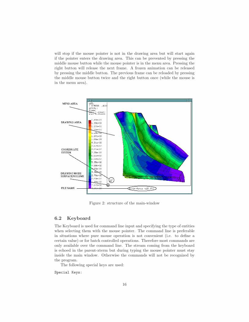
will stop if the mouse pointer is not in the drawing area but will start againif the pointer enters the drawing area. This can be prevented by pressing themiddle mouse button while the mouse pointer is in the menu area. Pressing theright button will release the next frame. A frozen animation can be releasedby pressing the middle button. The previous frame can be reloaded by pressingthe middle mouse button twice and the right button once (while the mouse isin the menu area).
Figure 2: structure of the main-window
6.2 Keyboard
The Keyboard is used for command line input and specifying the type of entitieswhen selecting them with the mouse pointer. The command line is preferablein situations where pure mouse operation is not convenient (i.e. to define acertain value) or for batch controlled operations. Therefore most commands areonly available over the command line. The stream coming from the keyboardis echoed in the parent-xterm but during typing the mouse pointer must stayinside the main window. Otherwise the commands will not be recognized bythe program.
The following special keys are used:
Special Keys:
16
ARROW_UP: previous command
ARROW_DOWN: next command
PAGE_UP: entities of previous set (if the last command was
plot or plus) or the previous Loadcase
PAGE_DOWN: entities of next set (if the last command was
plot or plus) or the next Loadcase
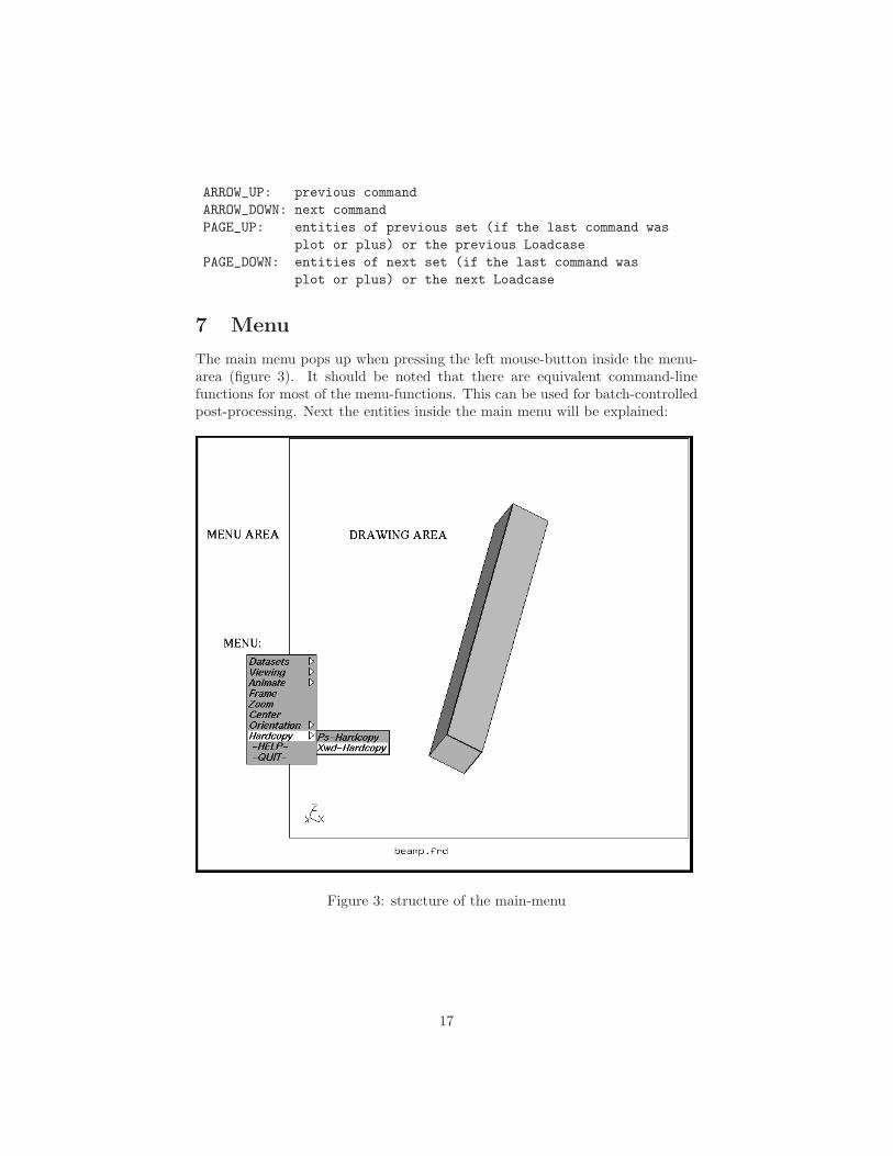
7 Menu
The main menu pops up when pressing the left mouse-button inside the menu-area (figure 3). It should be noted that there are equivalent command-linefunctions for most of the menu-functions. This can be used for batch-controlledpost-processing. Next the entities inside the main menu will be explained:
Figure 3: structure of the main-menu
17

7.1 Datasets
Datasets are selected with the menu-item ”Dataset”. A dataset is a block ofnodal values. These could be displacements due to a linear analysis or fora specific time-step during a nonlinear analysis. It could also contain othervalues like stresses, strains, temperatures or something else. To select a dataset,make sure that the mouse-pointer is inside the menu area. Then, press the leftmouse button and move the mouse-pointer over the menu entry ”Dataset”, thencontinue to the right. A sub-menu pops up showing all available datasets witha leading number and sometimes followed by a dataset-value (usually time orfrequency) and a dataset-description. Move the mouse-pointer over a datasetyou are interested in and release the left mouse button. The dataset is nowselected. A results ”Entity” must be chosen to see the values in the drawing-area. This Dataset might also contain automatically calculated values like thev. Mises stress and the maximum principal stress (see Pre-defined Calculationsand Result Format). See also the command ”ds” to control the functionalitywith the command-line.
7.1.1 Entity
To view data from the dataset, its also necessary to specify the entity (i.e. dx fora displacement Dataset). It works in the same way as for selecting the datasetbut instead of releasing the left mouse button over a Dataset continue to thebottom of the sub-menu to ”Entity.” Continue from that item to the right andrelease the mouse button when the pointer is over an entity. Now the data isdisplayed in the drawing-area.
7.2 Viewing
In the following sections, changing properties and styles of the displayed struc-ture are explained. See the command ”view” to control the functions with thecommand-line.
7.2.1 Show Elements With Light
This is the default view of the mesh if the program was started in viewing mode.If used, any animation will be interrupted and no values are displayed.
7.2.2 Show Bad Elements
This option presents elements which have a negative Jacobian value at least atone integration point. The solver ccx can not deal with those elements. So far,only TET and HEX elements are checked. These elements are stored in the setcalled -NJBY. See also the command ”eqal”.
7.2.3 Fill
This is the default mode and forces the element faces to be rendered.
18
7.2.4 Lines
The edges of the element faces are displayed. This is especially useful to see intothe structure to find hot spots in the displayed field. With ”Toggle Move-Z/Zoom”and ”qcut”, a more detailed analysis can follow. For very dense meshes switchto ”Dots”.
7.2.5 Dots
The corners of the element faces will be displayed. This is especially useful ifvalues inside the structure need checked.
7.2.6 Toggle Culling Back/Front
This removes the faces of volume elements for all elements or for the surface ofthe structure, depending on the state of ”Toggle Surfaces/Volumes”. With thisoption, the user can visualize internal structures like cracks or a core of a hollowstructure.
7.2.7 Toggle Illuminate Backface
Initially only the front faces are illuminated and the back faces are dark. Thisis helpful to determine the orientation of the elements. If you want to see allfaces illuminated regardless of the orientation, then use this option. If you wantto change the orientation of elements use the command ”qflp”.
7.2.8 Toggle Model Edges
Per default, all free element edges are shown. The user can remove/show themwith this option.
7.2.9 Toggle Element Edges
Per default, just the free element edges are shown. The user might add all edgesto the structure with that option.
7.2.10 Toggle Surfaces/Volumes
This switches the way each volume elements are displayed. Either all facesof the elements or just the element faces on the surface of the structure aredisplayed. Depending on the state of ”Toggle Culling Back/Front,” either thefaces pointing to the user or the faces pointing away are displayed. The defaultis just to show the surface pointing to the user. In the lower left corner of thedrawing area,(see figure 2) a character is printed, indicating the program is inthe surface mode ”s” or in the volume mode ”v”.
19

7.2.11 Toggle Move-Z/Zoom
Instead of zooming in with the help of the middle mouse button, it is alsopossible to move a clipping plane through the structure to get a view of theinside. The clipping plane is parallel to the screen and will be moved in thedirection to and from the user by pressing the middle mouse button and movingthe pointer up and down while inside the drawing area. Usually it needs somemouse movements until the clipping plane has reached the structure. Dependingon hardware, this functionality could be slow. After zooming in, consider usingthe ”plot” and ”plus” commands to customize your view.
7.2.12 Toggle Background Color
With this option, it is possible to switch between a black and a white back-ground.
7.2.13 Toggle Vector-Plot
It is possible to add small ”needles” to the plot which point with their headsin the direction of the vectors. Only entities which are marked in the databaseas vectors will be affected. See ”Nodal Results Block” for information on howentities are marked as vectors. Internally calculated vector-results, like the worstprincipal stress, are marked automatically. If one component or the value of avector is selected, then the option takes immediate effect.
This option can be used in combination with ”Animate Toggle Dataset Sequence”.
See also the keyboard command ”ds” how to select datasets and entities withthe keyboard. In this case, entities which are NOT marked in the dataset asvectors can be displayed with vector-needles. This command line approach with”ds” is the only way to display duns-cfd-results with vector-needles. See alsothe command ”scal” how to manipulate the length of the vectors.
7.2.14 Toggle Add-Displacement
It is possible to display results on the deformed structure. For example, youcan display a stress field on the deformed structure. If you know a suitableamplification factor for your displacements then use the ”scal” command toissue this value but this can also be done later. Of course displacements for theLoadcase must be available.
7.2.15 Toggle Shaded Result
It is possible to display results with illumination. For example, you can displaya stress field with a shaded appearance to have a better impression of the shapeof the structure.
20
7.3 Animate
This option allows the animation of displacements. See also ”anim”, ”ds” and”scal” to use this functionality with the command-line.
It is possible to create this sequence from just one Dataset, see ”Start”.This is useful for displaying mode-shapes. See also ”Toggle Dataset Sequence”to create a sequence from multiple Datasets to visualize dynamic responses.
7.3.1 Start
Creates a sequence of display-lists to visualize displacements (for example mode-shapes). The program recognizes displacements just by the name of the dataset.This name must start with the letters ”DISP”, otherwise the animation will notstart (see ”Nodal Results Block”).
7.3.2 Tune-Value
Controls the amplitude of the animation. If ”Toggle Real Displacements” waschosen before, the tune-value is equivalent to the amplification of the animation.
7.3.3 Steps per Period
Determines how many display lists for one period of animation will be used. If”Toggle Dataset Sequence” was chosen, then these number of display lists willbe interpreted as one period (see Time per Period).
7.3.4 Time per Period
Determines how many seconds per period.
7.3.5 Toggle Real Displacements
To see the correct displacement of each node. The animation can be controlledwith the help of the mouse.
7.3.6 Toggle Static Model Edges
The user can switch on additional undeformed model edges. This is usefull forhardcopies were this edges give a reference to the undeformed shape.
7.3.7 Toggle Static Element Edges
The user can switch on additional undeformed element edges. This is usefull forhardcopies were this edges give a reference to the undeformed shape.
21

7.3.8 Toggle Dataset Sequence
Creates a sequence of display-lists to visualize values of a sequence of Datasets.The Datasets must use the same type, for example only displacements or onlystresses. To activate the animation, after you have selected “Toggle DatasetSequence” choose the first Dataset to be displayed, then the second and thenthe last one. Finally choose the entity. The first two datasets define the spacingbetween the requested datasets and the third-one defines the last dataset to bedisplayed. The last two selections of datasets can be omitted. Then all datasetswhich use the same name, starting from the selected one, will be used. Thecommand ”ds” provides the same functionality.
7.4 Frame
Adjusts the drawing box.
7.5 Zoom
Use this command to zoom into a rectangular section of the window. After thisoption is chosen, use the mouse to select the opposite corners of a rectangle.The display will zoom in on the rectangular area. Note the rectangle is nevershown on the screen (see also ”zoom”).
7.6 Center
Used to choose a new center point for the structure. After this option is chosen,pick either a node, a point or the corner of an entity. To easily find the elementcorners, the function ”Toggle Element Edges” is triggered automatically (seealso ”qcnt”).
7.7 Enquire
Used to investigate parameters like the value and the position of a certain nodeof the model. Pick a node after this option is chosen. To easily find the elementcorners, the function ”Toggle Element Edges” is triggered automatically (seealso ”qenq”).
7.8 Cut
Used to cut elements and to create a section of new elements and nodes. Eitherpick three nodes, or, in case a dataset-entity of a vector was already selected,use the menu entry “vector” and select just one node. The cutting plane isthen determined by the direction of the selected vector (displacements, worstPSetc.). To easily find the element corners, the function ”Toggle Element Edges”is triggered automatically (see also ”qcut” and ”cut”)
22

7.9 Graph
Used to generate a 2D-plot. The option “Length” will provide a plot “valueover distance between nodes”. The option “Datasets” will provide a plot “valueover Dataset-nr” and the option “Time” will provide “value over Time”. Forthe later two options it is necessary to first create an animation with either thecommand ”ds” or the menu option ”Toggle Dataset Sequence” (see also ”graph”and ”How to generate a time-history plot”). To easily find the element corners,the function ”Toggle Element Edges” is triggered automatically.
7.10 User
This menu item does not exist until the first ”menu” command was executed.Each “menu” command adds a new user command to the menu. This “menu”commands are usually stored in a “.cgx” file in the home directory to link themto the menu during startup.
7.11 Orientation
7.11.1 +x View
To look along the x-axis.
7.11.2 -x View
To look against the x-axis.
7.11.3 +y View
To look along the y-axis.
7.11.4 -y View
To look against the y-axis.
7.11.5 +z View
To look along the z-axis.
7.11.6 -z View
To look against the z-axis.
7.12 Hardcopy
To create a hard-copy during animation, it is useful to stop the animation firstwith the middle mouse button while inside the menu area of the main windowand then release one picture after the other with the right button until thedesired amplitude or step is reached.
23

7.12.1 Tga-Hardcopy
To create a window dump in tga format. You might use the program ”convert”[11] to convert this format to others.
7.12.2 Ps-Hardcopy
To create a window dump in postscript format. The program convert must beinstalled.
7.12.3 Gif-Hardcopy
To create a window dump in gif format. The program convert must be installed.
7.12.4 Png-Hardcopy
To create a window dump in png format. The program convert must be installed.
7.12.5 Start Recording Gif-Movie
All frames during an animation are stored. The recording ends after the rightmouse button is pressed while in the menu area. Finally all frames are combinedin the file ”movie.gif” which can be displayed with various tools (Firefox [12] orrealplay). If the animation is stopped with the middle mouse button while inthe menu area, then the movie stops until it is released by pressing the middlemouse button again. See ”movi” for the keyboard options. Further remarks in”How to change the format of the movie file”.
7.13 Help
Starts the html help and displays this document. It only works if the specifiedhtml-viewer is available. The default is Firefox [12] but this can be changedin the ”cgx.h” file. The search-path for the documentation is also defined inthe ”cgx.h” file. Please make sure that the documentation is in the speci-fied location or change the path in the ”cgx.h” file and recompile the pro-gram after the object-files are deleted. The default location for the html helpis .../CalculiX/cgx X.X/doc/cgx and /CalculiX/ccx X.X/doc/ccx for cgx andccx respectively. The html files must be downloaded directly or compiled fromthe latex source for this function to work properly. The INSTALL file tellshow to compile the latex code to html. The INSTALL file is located .../Cal-culiX/cgx X.X/ and .../CalculiX/ccx X.X/ for cgx and ccx respectively.
7.14 Quit
This terminates the program without a save.
24
8 Customization
The file “.cgx” located in the $HOME directory will be read at program start.The following commands might be usefull in this context:
• ”font”
• ”menu”
• ”rot”
• ”view bg”
• ”view sh”
• ”wpos”
• ”wsize”
Example content of a “.cgx” init file:
valu vinp /home/user/cgx_templates/readinp.fbl
menu readinp(vinp) read vinp
9 Commands
This section is a reference to all commands and their parameters in alphabeticorder. If a command is typed the mouse-pointer must be in the main window(figure 2). Only the echo of the input stream is visible in the parent xterm. Thekeywords are not case sensitive but all command parameters are case sensitive.Each reference starts with a short description of the command. The followingsyntax is used for these descriptions:
Known commands and syntax:
’..’: Keyword (either uppercase or lowercase)
<..>: Parameter (case-sensitive)
[..]: combination of parameters or optional parameter
(..): Remark
| : OR
& : AND
- : from-to
-> : command continues in the next line
RETURN press the RETURN key
Entities—with the exception of nodes and elements—are referenced by nameswhich can contain letters and numbers. Usually one to four characters is rec-ommended. If a new entity uses an existing name, the old definition will beoverwritten. To overcome this problem, ”alias” names can be used. An aliasname is defined with the ! sign in front. An already defined alias name can be
25
referenced by placing the % sign in front. For example:
LINE !L1 %P1 %P2 %SET
will create a line with the alias name L1 and will use the alias names P1 andP2 to define the end-points and uses the set SET to define the point sequencebetween the end-points. The assigned alias name for a given entity can beenquired with a leading question mark using the prnt command.
9.1 anim
’anim’ ’tune’ <value>|’steps’ <value>|’time’ <value>|->
’real’ [’on’|’off’]|’model’ [’on’|’off’]| ->
’elem’ [’on’|’off’]| ’start’
This keyword is used to manipulate the animation of displacements. See also”ds” and ”scal”. The amplification is controlled with “tune”. “steps” defines thenumber of frames over one periode. “time” controlls the duration of one periode.“real” switches of the automatic amplification and the real displacements areused instead. In addition the displacements of the negative part of the periodeis set to zero. “model” switches the static model (undeformed) edges on or of.“elem” does this for the element edges. Start the animation with ’start’. Theanimation stops when using the ’ds’ or the ’view’ commands with appropriateparameters.
9.2 area
’area’ <set>
This keyword is used to calculate the area and the center of gravity of a set ofshell-elements or surfaces of volume-elements. If a ’dataset’ is active then anaveraged value is calculated.
It averages the nodal values per element and weight it (multipies it) withthe area of that element. The sum of all the weighted element-values is thendivided by the total area of all regarded elements. The center of gravity is alsoweighted with the indvidual areas. This works for faces as well. In case the”qcut” command was used to create a section it is necessary to use the ”comp”command to add the related faces to the set ’-qcut’ which holds the section:
comp -qcut do
Then the ’area’ command can be used:
area -qcut
which produces a listing like that:
26

AREA:98.437740 CENTER OF GRAVITY: 9.214960 0.663785
24.655288 AVERAGE-VALUE:252.453576
The command writes to the ”stack”.
9.3 asgn
’asgn’ [’n’|’e’|’p’|’l’|’c’|’s’|’b’|’S’|’L’|’se’|->
’sh’|’alpha’|’beta’|’nadapt’ <value>] | ->
[’rbe’ <value>|’mpc’]
This keyword is used to manipulate the behaviour of successive commands.For example to define the first node or element number which will be used
for the next mesh generation. And it is used to redefine the leading characterof new entities. The default is D for points p, L for lines l, C for combined lines(lcmb) c, A for surfaces s, B for Bodies b, Q for nurb lines (nurl) L, N for nurbsurfaces (nurs) S, A for sets se and H for Shapes sh. For example
asgn p U
will assign the character U as the leading character to all newly created namesof points. The automatically created names of geometric entities use 4 charac-ters. If all possible names with the chosen leading letter are in use then the nextalphabetical letter is chosen as a leading letter, so after PZZZ follows Q000. Ifno more letter follow then the amount of letters per name is increased. Themaximum number is 8. Each entity has its own name-space. Different entitiesmight use the same name. Remark: Currently nurbs-lines are automaticallyused to create splines sharing the same name. Nurbs-lines can not be used forother purposes than to be displayed and so far they can not be written to a file.
The command is also used to controll the behaviour of the unstructuredtriangulator. This unstructured mesher [14] uses the tree parameters alpha,beta, nadapt for mesh-control. Current default is 0.4 for alpha and beta and 4for nadapt.
In case Nastran input should be generated it is possible to switch from MPCsto RBEs when using the send command in combination with the areampc op-tion. The value after “rbe” represents the thermal expansion coefficient of thiselements:
asgn rbe 0.5e-6
It should be noted that coincident nodes are connected by MPCs either way.
9.4 bia
’bia’ <line>|<set> [ [<bias>] [<factor>]|
[’mult’|’div’ <factor>] ]
27

This keyword is used to define the bias of a single line or of a set of lines (seeqadd). The bias defines the ratio of the length of the first element to the lengthof the last element. For example,
bia all 4.5
will force a ratio in which the last element is 4.5 times bigger than the firstone. Real numbers are permitted since version 1.5 (see also qbia). To convertfrom pre 1.5 versions, start the program with the -oldbias option. A negativefactor permits to invert the direction of the bias:
bia all 4.5 -1
9.5 body
’body’ <name(char<9)>|’!’ [<surf1> <surf2>]|
[<surf1> <surf2> <surf3> <surf4> ->
<surf5> [<surf6> <surf6>]]|
[<set>]
This keyword is used to define or redefine a volume (body). Each body musthave five, six or seven surfaces to be mesh-able with hexaeder-elements, oth-erwise it can only meshed with tets if NETGEN [4] is installed. However, itis sufficient to specify just the ”top” and the ”bottom” surfaces. But if sur-faces with 3 or 5 edges are involved then this surfaces have to be the ”top” and”bottom” surfaces. This is also true if surfaces have different line-divisions atopposite edges. The missing surfaces between the ”top” and ”bottom” surfaceswill be created automatically if they do not already exist (they will always have4 edges with the same division on opposide edges). But all needed lines mustexist. More precisely, only single lines or existing combined lines (lcmb) can bedetected. The user must define the missing surface if just a chain of lines (andno lcmb) is defined between two corner points of the ”top” and ”bottom” sur-faces before he can successfully use the body command. It is a more convenientway to define a body than the command “gbod” but exactly 2 or all surfacesmust be specified otherwise the body will not be created (The most convenientway to define bodies is to use the command “qbod”). For example,
body b1 s1 s2
will look for the missing surfaces and if necessary create them if all lines betweenthe corner points of s1 and s2 are defined; the result is the creation of body, b1.Or for example,
body ! s1 s2 s3 s4 s5
28
will create a body and a new name for it. The new name is triggered by thesign !. Here the body is based on 5 surfaces. If the surfaces are not connected,the body is not mesh-able.
In case a body should only be meshable with tets it can be composed of morethan 7 surfaces. The definition can be provided by a set of surfaces:
body ! surfset
will create a body based on the surfaces referenced by surfset.
9.6 break
’break’
This keyword is used to end the interpretation of a command file. The programreturns to the interactive mode.
9.7 call
’call’ <parameters>
This keyword is used to allow the user to control his own functionality in the file”userFunction.c”. The data-structures for the mesh and datasets are available.The default function calculates the hydrodynamic stresses with the command:
call hydro
See ”User-Functions” for details.
9.8 cntr
’cntr’ <pnt|nod|set>|[x y z]
Defines a new rotation center. See also ”qcnt” for the cursor controlled com-mand.
9.9 comp
’comp’ <set|*chars*> ’u’|’d’|’e’
This keyword is used to add all entities to the specified set (see seta) which de-pend on the already included entities (u, up), or to include all entities necessaryto describe the already included entities (d, down).For example the set ”lines” stores lines and should also include all dependentpoints:
29

comp lines do
Or the set ”lines” should also include all surfs and bodies which depend onthe lines:
comp lines up
In some cases you will need only the end-points of lines. With the option(e, edges)
comp lines e
only end-points are included in the set. One exception to this logic was in-troduced for convenience:
comp nodes do
will add all faces described by the nodes in set nodes despite the fact thatfaces are made from nodes.
Wildcards (*) can be used to search for setnames of a certain expression:
comp E* do
will complete all sets starting with “E”.
9.10 copy
’copy’ <set> <set> [’scal’ <fx> <fy> <fz> <pnt> [a] ]|
[’tra’ <dx> <dy> <dz> [a]]|
[’rot’ <p1> <p2> <alfa> [a] ]|
[’rot’ ’x’|’y’|’z’ <alfa> [a] ]|
[’rot’ <p1> ’x’|’y’|’z’ <alfa> [a] ]|
[’rad’ <p1> <p2> <dr> [a] ]|
[’rad’ ’x’|’y’|’z’|’p’<PNT> <dr> [a] ]|
[’rad’ <p1> ’x’|’y’|’z’ <dr> [a] ]|
[’nor’ <dr> [a] ]|
[’mir’ <P1> <P2> [a] ]|
[’mir’ ’x’|’y’|’z’ [a] ]|
[’mir’ <P1> ’x’|’y’|’z’ [a] ]
This keyword is used to create a copy of a set (see seta about sets). Geometry,nodes and elements with their results can be copied. The copy of results isusefull to evaluate additional sectors in case of a cyclic symmetric calculation.The copy is included in the new set. Existing sets are extended by the copiedentities if the last parameter “a” (append) is provided. Several transformations
30

are available. For example scal creates a scaled copy, the scaling factors fx, fy,fz can be chosen independently,
Several transformations are available. For example scal creates a scaled copy,the scaling factors fx, fy, fz can be chosen independently,
copy part1 part2 scal 2 P0copy part1 part2 scal 1 1 2 P0
tra will create a copy and will move it away by the vector dx, dy, dz andthe optional parameter a will assign the new entities to sets were the mother ofeach entity is included,
copy set1 set2 tra 10 20 30 a
rot will create a copy and will move it around the axis defined by the points p1and p2 by alfa degrees,
copy set1 set2 rot p0 px 20.
or the axis of rotation is given by specifying one of the basis coordinate axes:copy set1 set2 rot x 20.
or just one point and a vector of rotation is given by specifying one of thebasis coordinate axes: copy set1 set2 rot p1 x 20.
rad will create a copy and uses the same transformation options as ’rot’ orwill create a spherical section if just a single point is defined,
copy sphere1 sphere2 rad pP0 10.
nor will create a copy and will move it away in the direction of averaged nor-mal local vector. This requires information about the normal direction for eachentity. Nodes will use associated element faces and geometric entities will usethe element faces, surfaces or shapes which are stored with them in the set1,
copy set1 set2 nor 1.2 a
mir will create a mirrored copy. The mirror-plane is placed normal to thedirection running from P1 to P2 and placed at P2,
copy section1 section2 mir P1 P2.
as with ’rot and ’rad’ additional transformation options are available:
copy section1 section2 mir P1 x
31

places the mirror at P1 with its normal direction in ’x’ direction
copy section1 section2 mir x
Places the mirror in the origin with its normal direction in ’x’ direction.
9.11 corrad
’corrad’ <set>
This is a very special command to adjust improperly defined arc-lines, like infillets. The center points of arc-lines included in the set are moved in a way thateach arc-line will run tangentially into a connected straight line. But becausethe end-points of the arc-lines are not moved only one side of each arc-line willrun into a connected line. The other side is not controlled and might end ina sharp corner. Therefore for each arc-line exactly one connected straight linemust be included into the set (figure 4).
Figure 4: Effect of the corrad command
9.12 csysa
’csysa’ <sysNr> <set>
Specifies the displacement coordinate system for each node (Nastran only).
32

9.13 cut
’cut’ <pnt|nod> [<pnt|nod> <pnt|nod>]
This keyword is used to define a cutting plane through elements to visualizeinternal results. The plane is either defined by three nodes or points, or, incase a dataset-entity of a vector was already selected, by just one node or point.The cutting plane is then determined by the direction of the vector (displace-ments, worstPS). The menu option ”Show Elements With Light” or the com-mands ”ucut”, ”view surf” or”view volu” will display the whole model again andwill delete the plane. This command is intended for batch-mode. See ”qcut”for the cursor controlled command.
9.14 del
’del’ [’p’|’l’|’l0’|’c’|’s’|’b’|’t’|’S’|’L’|’se’|’sh’ <entity>]|
[’se0’]|
[’mesh’]|
[’pic’]
This keyword is used to delete entities, the whole mesh (see also qdel) or abackground-picture. For example,
del se part
will delete the set “part” but all included entities are untouched. The followingentities are known:
Points p, Lines l, Combined Lines c, Surfaces s, Bodies b, Node Texts t, NurbSurfaces S, Nurb Lines L, Sets se and Shapes sh.
When an entity is deleted, all dependent higher entities are deleted as well.Special cases are
del l0 set (l¡zero¿)
were all lines with zero length in set ”set” are deleted and
del se0
will delete all empty sets. If a background-picture was loaded with the ”read”command it can be deleted with:
del pic
See also ”zap” on how to delete a set with all its referenced entities.
33
9.15 dist
’dist’ <set> <target-set>|<shpe> ->
[’tra’ <dx> <dy> <dz> <offset>]|
[’rot’ <p1> <p2> <offset>]|
[’rot’ ’x’|’y’|’z’ <offset>]|
[’rad’ <p1> <p2> <offset>]|
[’rad’ ’x’|’y’|’z’ <offset>]|
[’nor’ <offset> <tol>]
measures distances between entities of two sets. For example between points ornodes stored in one set to surfaces or shapes stored in a second set. The average-, maximum- and minimum distance is determined. The distance is measurednormal-, rotational-, radial or translatoric. The command works analogous tothe ”proj” command. Please look there for details.
The command writes to the ”stack”.
9.16 div
’div’ |
<defdiv>|
<line> [<division>]|
<set> [<division>]|
[’mult’|’div’ <factor-div> <factor-bias>]|
[’auto’ <node-dist> <angle> <elem-ratio>]
This keyword can be used to re-define the default division of lines:
div 4
The div keyword works on a line or a set of lines (see qadd). The divisioncontrols the number of nodes created when the geometry is meshed (see eltyand mesh). For example,
div all 4
attaches the division of 4 to all lines. With the keyword mult or div in combi-nation with a value, it is possible to multiply or divide already assigned divisions:
div all mult 2.
Or in case you need a starting-point for the individual divisions you can usethe option auto with the optional parameters node-dist and angle. Node-distis the maximum allowed distance between nodes and angle is the maximum al-lowed angle defined by three sequential nodes. If one parameter is not fulfilledthen the division is halved until the requirements are fulfilled. Default valuesare defined in the file cgx.h and can be listed with
34
div
without parameters
div all auto
uses the defaults. But they can be overruled
div all auto 2. 10. 0.5
will use a maximum element lenght of 2., the angle between successive nodesis less than 10 degree and the minimum element is only half of the maximum-length.
9.17 ds
’ds’ [<1.Dataset-Nr> [<2.Dataset-Nr>] [<n.Dataset-Nr>] ->
[’a[h]’|’e[h]’ [<entity-nr> (up to 4 times)]]|
[’o’ <value> [<entity-nr>]]|
[’p’ <power> [<entity-nr>]]|
[’s’ <value> [<entity-nr>]]|
[’r’ <key> [<parm1>] [<parm2>] [..<parm5>]]]|
[’g’ <name> [[<ncomps>|<0>] <value> <text> <type> ->
<step> <analysisName>]]|
[’e’ <name> <comp> <type> <row> <column>]
This keyword is used to select, modify or generate one or more Datasets (ds)and one or more Entity (e). In addition it can be used to generate or modifyrelated parameters which might store step specific descriptions. The dataset hasto be a positive number which has to match the nr in the Dataset-menu or an ’l’(lower case ’L’) which is interpreted as the last available Dataset or a negativenumber. Then it is interpreted as the last ds minus the specified number. Forexample
ds 1 e 1
will display the first entity of the first Dataset.
ds l e 1
will display the last Dataset. To start the animation of the second-to-lastDataset right away:
ds -1 a
35
Or generate an animated fringe plot by adding the desired entity:
ds -1 a 4
Sequences can be defined by specifying one to three datasets and by extend-ing the ’e’ parameter by an ’h’ (’history’):
ds 2 eh 1
Here all datasets of the same type as ds 2 are selected. The spacing betweendatasets of the same type is only evaluated for the first step. A unique step-withis therfore needed.
ds 2 10 eh 1
Here the datasets 2, 10 and all successive ones of the same type with a spacingof 8 are selected.
ds 2 4 10 eh 1
Here the 1st entity of each second Dataset is selected. The selection startsat the second- and ends at the 10th dataset. If more than one entity is definedthen a vector-plot will be displayed. If a 4th entity is defined then this entitywill be used for the basic color-plot:
ds 2 4 10 eh 12 13 14 15
In case the deformed shape should be shown together with the fringe plot in asequence of datasets then the ’e’ parameter has to be replaced by an ’a’ char-acter.
ds 2 ah 1
REMARK: So far vector plots can not use the deformed shape. Thereforeonly one entity is supported.
In addition, it is possible to scale or offset the entities of the specified datasets:
ds 1 s 1.2
will scale all entities of dataset 1 by a factor of 1.2.
ds 1 p 1.2 3
will use the given exponent to scale entity 3 of dataset 1 by an exponent of1.2.
36
ds 1 o 200.
will add a value of 200 to all entities of dataset 1.
ds 1 o 200. 2
will add a value of 200 to the entity 2 of dataset 1. Each dataset might userelated parameters (see Parameter Header Record for the format of a parame-ter record). This parameters can be overwritten or created:
ds 2 4 10 r TAMB 1
Each second dataset from 2 to 10 gets a related parameter ’TAMB’ with thevalue ’1’. If the value is nummeric it can be used by the “graph” command.
A new dataset in which all values are initiallized to zero is generated with:
ds g VELOCITY 3
The ’name’ VELOCITY will appear in the menu as the dataset name and canbe 8 character long. It has 3 components (’ncomps’, default is ’1’). The otherparameters are optional:
• value: A nummeric value, usually time or frequency (used by “graph”).
• text: A describing text (used by “graph”).
• type: Analysis type (static:0,time step:1,frequency:2, etc.).
• step: Step or increment number
• analysisName: Type of analysis (description).
The current dataset name is modified if only the name is given:
ds g VELOCITY
The other parameters of the current dataset can be modified if the numberof components is set to zero: ds g VELOCITY 0 1e4 test
The entities of the current dataset are manipulated with:
ds e V 2
The ’name’ V will appear in the menu as the entity name and can be 8 characterlong. It is the second entity of the current dataset (’comp’, default is ’1’). Theother parameters are optional:
37

• type: Mathematical data type (scalar:1, vector:2, matrix:4, etc.)
• row: sub-component index or row number
• column: column number if matrix
The values at the nodes are manipulated with the ”node” command. Thisshould happen before the ’ds e’ command is used since that command does alsodetermine the maximum and minimum values used in the graphical window.More details can be found in section ”Nodal Results Block”.
9.18 elem
’elem’ <nr|!> [set]|
[<firstNode> .. <lastNode> ’be2’|’be3’|’tr3’|’tr6’|->
’qu4’|’qu8’|’he8’|’he20’]
This keyword is used to define elements based on nodes and its type (see sectionElement Types in the appendix for the correct node-order). For example,
elem 1 1 2 3 4 qu4
creates a shell element with four nodes. If the an automatically generated nameis desired, then type ”!” instead of a name. Shell elements can be created basedon a set of element-faces:
elem ! faceset
This might be usefull to create a layer of shell elements on volume elements.
9.19 else
’else’
See the “if” command.
9.20 elty
’elty’ <set> ’be2’|’be2f’|’be2d’|’be3’|’be3f’|->
’tr3’|’tr3u’|’tr3e’|’tr3s’|’tr3c’->
’tr6’|’tr6u’|’tr6e’|’tr6s’|’tr6c’|->
’qu4’|’qu4e’|’qu4s’|’qu4c’|->
’qu4r’|’qu4er’|’qu4sr’|’qu4cr’|->
’qu8’|’qu8e’|’qu8s’|’qu8c’|->
’qu8r’|’qu8er’|’qu8sr’|’qu8cr’|->
’he8’|’he8f’|’he8i’|’he8r’|->
’he20’|’he20r’|’pe6’|’pe6f’|’pe15’|->
’pe15r’|’te4’|’te4f’|’te10’|’te10m’|->
’te10t’ [<parameter>]
38

This keyword is used to assign a specific element type to a set of entities (seesection Element Types in the appendix). In most cases it can be used to specifythe element type before the mesh is created. In case of unstructured meshes theelement attributes have to be assigned after the mesh is created (from tr6u totr6c or te10 to te10t etc.).
The element name is composed of the following parts: The leading twoletters define the shape (be: beam, tr: triangle, qu: quadrangle, he: hexahedra,pe: penta, te:tetraeder), then the number of nodes and at last an attributedescribing the mathematical formulation or other features (c: axisymmetric,e: plain strain, s: plain stress, u: unstructured mesh, r: reduced integration,i: incompatible modes, f: fluid element for ccx, t: initial temperatures areinterpolated linearly within the tet element (ccx:C3D10T)).
If the element type is omitted, the assignment is deleted. If all parametersare omitted, the actual assignments are posted:
elty
will print only the sets with assigned elements. Multiple definitions are pos-sible. For example,
elty all
deletes all element definitions. If the geometry was already meshed, the meshwill NOT be deleted. If the mesh command is executed again after new assign-ments has taken place, additional elements will be created.
elty all he20
assigns 20 node brick-elements to all bodies in the set all.
elty part1 he8
redefines that definition for all bodies in the set part1.
elty part2 tr6u
assigns 6 node unstructured triangle elements to all surfaces in set part2.
elty part2 tr6u 0.5
will do the same but specifies a mesh refinement factor of 0.5 (>1: coarserthan the average boundary spacing, <1: denser ). Be aware that specializedunstructured meshes must be created by using two times the elty command.First time the general unstructured type before the mesh is actually createdand afterwards a redefinition into the more specific type:
39
elty part2 tr6umesh allelty part2 tr6c
creates an axisymmetric unstructured mesh.
elty part3 te10
assigns 10 node elements to all bodies in set part3. But this works only ifNETGEN [4] is installed and the program ng vol is accessible.
elty part3 te10 3.5
will do the same but specifies a target size for the elements. In this case themodified program ng vol from the cgx-distribution must be available. Replacethe original ng vol in the NETGEN package and build it again. Be aware thatspecialized unstructured meshes must be created by using two times the eltycommand. First time the general unstructured type before the mesh is actuallycreated and afterwards a redefinition into the more specific type:
elty part2 te10mesh allelty part2 te10t
The penta element types are not supported for meshing but can be used toredefine the attributes (pe6 to pe6f). Penta elements are only created if a meshof triangles (2D) is sweeped in 3D. This procedure is used to create quasi 2Dcfd meshes.
The fluid network element types are be2f and be3f. The be2f has to be usedat the begin and the end of a network. This elements will use the special node nr’0’ at the entry and exit. This node-nr is automatically assigned to the elementdefinition when written in the ccx format. All other elements in the networkmust use the be3f type. The detailed element type definition has to be done inthe ccx input file based on element-sets.
9.21 endif
’endif’
See the “if” command.
9.22 endwhile
’endwhile’
See the “while” command.
40

9.23 enq
’enq’ <set> <set> [’set’ <setname> ]|->
[’rec’ <x-value>|’_’ <y-value>|’_’ <z-value>|’_’ ]|->
[’cx’|’cy’|’cz’ <r-value>|’_’ <fi-value(deg)>|’_’ ->
<axis-value>|’_’ ] ->
<tol> ’i’|’a’|’h’|’l’ [<value>]
This command is used to locate entities from a certain set (first provided set)and stores them in the second set. The following entities are handled: nodes,points, lines, surfaces. But surfaces can only be identified if the command “rep<setname>” was issued before. In case of nodes with related values (results)it will also determine the highes or lowest value in the specified range, or, allnodes above or below a certain value. The coordinates might be taken from onenode or point in a given 3rd set or given in cartesian coordinates (option rec) orcylindrical coordinates (option cx, cy, cz). Some coordinates might be omittedto specify an infinite range. The ’ ’ key has to be used in this case. The modeis defined by the keys ’i’ individual, ’a’ all, ’h’ high, ’l’ low, were h and l willsearch the highest or lowest value in range. This value will also be written to afile for automatic processing purposes. For example
enq all newset rec 10. 100. 0.1 i
will search for entities in set ’all’ at the given location x:10. y: (infinite range,triggered by the ’ ’ key) z:100. with a tolerance of 0.1 and only the closest entityof all kinds of entities are stored in set ’newset’, triggered by the ’i’ key. Withthe ’a’ key all in range would be stored. The key ’h’ or ’l’ would trigger a searchfor the highest or lowest value in the specified range.
In combination with a certain value
enq all newset rec 10. 100. 0.1 h 1013.
all nodes with a value above “1013.” would be stored in set “newset”. Thecommand
enq domain1 newset cx 100. 180. 10. 0.1 a
will search for entities in set ’domain1’ at radius:100. around x at fi:180 de-gree and x:10. with a tolerance of 0.1. All entities in range are stored in set’newset’.
The following example illustrates the use of “enq” to find the highest valueclose to a location given by a node-number:
# activate dataset 3 with entity 7:
ds 3 e 7
# read a file with one node to define a set:
read pos1.frd pos1
41

# search the highest value around a radius of 1:
enq all t set pos1 1. h
# move the file with the search result to a meaningfull name:
sys mv enq_lc3_e7_1.out pos1.out
The command writes to the ”stack”.
9.24 eprop
’eprop’ <set>
Calculates the element edge length and volume. Usefull for cfd meshing.
9.25 eqal
’eqal’ ’jbir’|’aspr’|’mca’ <value>
The keyword without parameters lists the current element quality thresholds(0==off):
• JBIR: The maximum ratio of jacobian determinants xsj between all gaus-points. Were xsj = Vworldcoordinates / Velementcoordinates and jbir =xsj-max / xsj-min. Supported element types he8, he20, te10.
• ASPR: Element aspect ratio between all element sides. Supported elementtypes he8, he20.
• MCA: Maximum corner angle between all element sides. Supported ele-ment types he8, (he20 as he8).
With parameter “value” sets the value of the threshold. The element-quality ischecked with ”plot eq all”.
9.26 exit
’exit’
This command terminates the program and saves the geometry (if any) to a filenamed as the input file but with the extension .fbd. If a file with that nameexists already, then this file will be saved with the new file extension .fbb as abackup (see also save).
9.27 fil
’fil’ <line> <line> <radius>
This command creates an arc of a given radius between the two specified lines.
42
9.28 flip
’flip’ [<set> <e>|<b>|<s>]|
[<s> [’auto’]]
This command changes the orientation of a set of shell-elements, bodies orsurfaces. In case of a single surface with the parameter “auto” all surfaces will beflipped in a way that they share a common direction (in or out of a volume). Therelated elements are also flipped. See qflp for the cursor controlled command.
9.29 flpc
’flpc’
This command changes the colour of the scale. Initialy the default is red forhigh values and blue for low values. The command will invert the current state.
9.30 font
’font’ ’d’|’l’ <value(1-6)>
This command changes the drawing-font. Six fonts of different heigh are avail-able:
font d 6
selects the highest font for the drawing area were
font l 1
selects the smallest one for the legend. The default is selected if no numberis specified:
font d or font l
9.31 frame
’frame’ [<setname>]
This command fits the model or the contents of a given set into the drawingspace.
When executing commands which increase the used space then it mighthappen that geometry is clipped and can not be seen or accessed anymore.This command is usually automatically triggered.
43

9.32 gbod
’gbod’ <name(char<9)>|’!’ ’NORM’ ’+|-’ <surf> ’+|-’ <surf> ->
.. ( 5-7 surfaces )
This keyword is used to define or redefine a body in the most basic way (see also“qbod”). Each body must have five to seven surfaces to be mesh-able. However,the number of recommended surfaces is six. The first two surfaces should bethe ”top” and the ”bottom” surfaces. For example,
gbod B001 NORM - S001 + S002 - S005 - S004 - S003 - S006
will create a body B001. The keyword ”NORM” is a necessary placeholderfor future functionallity but has no actual meaning. Next, follow the surfaceswith a sign ”+” or ”-” in front that indicates the orientation of each surface.These signs will be corrected automatically if necessary. If the an automaticallygenerated name is desired, then type ”!” instead of a name.
9.33 gonly
’gonly’ ’on’|’off’
This keyword is used to erase the contents of the menu area. Sometimes this isuseful for hardcopies.
9.34 graph
’graph’ [<amplitude|*chars*> ’amp’ [’l’]]|
[<material|*chars*> ’mat’ [’l’]]|
[<set|seq> ’length’ [’+’|’-’]]|
[<set>|’-p’ ’nr’|’time’|’descr’|<parameter-name> ->
[<Dataset-name> <entity-name>|<parameter-name> ] ->
[<first-Dataset-Nr> <last-Dataset-Nr>] ]
This keyword is used to create time history plots of nodal values. The valuesof the pre-selected nodes stored in the referenced set will be written to a filecalled ”graph.out”. A gnuplot command file will be written called ”graph.gnu”and executed. The resulting file ”graph.ps” will be automatically displayed withthe postscript viewer. The default is ”ghostview” but this can be changed in the”cgx.h” file before the program is build. See also “How to generate a time-history plot”for further details.
A set with the nodes of interest must be created (usually with “qadd”) be-fore a graph can be drawn. If the parameter l (length) is used to plot valuesalong the length of a set of nodes then this set should be of the sequence type(usually created with “qseq”):
graph seq length
44
The length is calculated as the sum of the distances between successive nodes.Un-ordered sets (as created with “qadd”) will be ordered in a way that thepositive direction points away from the origin of the coordinate system. Thedirection can be chosen with a ’+’ or ’-’ sign following the ’length’ parameter(’+’ is default).
Instead using existing nodes it is possible to use a line or a combined line“lcmb” as a method to generate new locations for data-points. The currentdisplayed results will be automatically mapped to this locations and shown ina 2D graph over the length of the line:
graph lineset length +
The set lineset stores a line. Since a ’+’ was given the graph starts at thebeginning of the line. With a ’-’ it would start at the end of the line.
Since version 1.8, there are two ways of operation. One way is to specify theDatasets and the entity as parameters of the command
graph set time DISP D1
which will display the displacement D1 of nodes in ”set” vs. the dataset-time ofall ”DISP” Datasets. The first and the last dataset can be specified optionally.
For the traditional way, a sequence of datasets must have been selected (seeToggle Dataset Sequence). After the selection of the datasets, an Entity mustbe specified. Then, the user could use the graph command to generate thehistory-plot of this pre-defined sequence. The command
graph set nr
will display the values on the node-positions vs. the dataset-numbers. Thecommand
graph set time
will display the values on the node-positions vs. the dataset-values (usually timeor frequency, see Nodal Results Block, parameter “VALUE”)) and the command
graph set descr
will display the values on the node-positions vs. the dataset-description (onlymakes sense if the description is a numerical value. See Nodal Results Block),parameter “TEXT”, for the location of this data in the frd-file.
In addition, a second data-file is written ”graph.out2” which stores the node-number and the node-coordinates and all values at this node-position for alldatasets. This file can be used to display values over node-positions, etc. It is
45

up to the user to generate a suitable plot out of this data.
The ”graph” files can be edited and combined. For example to plot one type ofvalue vs. another type of value.
If an ccx- or Abaqus-input-file was read then it is also possible to createtime history plots of the amplitudes (*AMPLITUDE in ccx) or the material-properties can be displayed (*MATERIAL in ccx):
graph amplitude-name amp
graph material-name mat
Wildcards (*) can be used to search for amplitudes or materials of a certainexpression. They are listed with all values if the parameter “l” follows after“amp” or “mat”:
graph *N* amp l
lists all amplitudes which contain the ’N’-key in its name with all values.The parameters related to datasets can also be displayed with the graph
command:
graph -p time DISP HID
This command plots the nodal-diameters used in a cyclic symmetry calcula-tion over the dataset-value. Only few parameters are written from ccx in frd-format. Other applications might define its own parameters in frd-format (seeParameter Header Record for the format of a parameter record). If needed cgxcan also create this dataset parameters, see the ”ds” command on how to do it.
9.35 grpa
’grpa’
This command allows to assign elements to a group. The group number is anelement attribute used in the frd file. That way the user can read an result file,define groups and store the results together with group-definitions for furtheruse in case no ccx input file is available. One element can only belong to onegroup. This command assigns a group number to certain elements stored in agiven set. See “Element Definition Block” how this applies to the result format(frd).
46
9.36 grps
’grps’
The result format (frd) allows to assign elements to a group. One element canonly belong to one group. This command creates sets and stores all elements of acertain group in a certain set called “+grp[nr]”. See “Element Definition Block”how this applies to the result format (frd).
9.37 gsur
’gsur’ <name(char<9)>|’!’ ’+|-’ ’BLEND|<nurbs>|<shape>’ ->
’+|-’ <line|lcmb> ’+|-’ <line|lcmb> .. (3-5 times)
This keyword is used to define or redefine a surface in the most basic way (seealso qsur). Each surface which is intended for a regular mesh must have threeto five edges which might consist of a single line or a combined line (see lcmb)to be mesh-able. However, the recommend amount of edges is four. For example,
gsur S004 + BLEND - L002 + L00E + L006 - L00C
will create the surface S004 with a mathematically positive orientation indicatedby the ”+” sign after the surface name. The keyword ”BLEND” indicates thatthe interior of the surface will be defined according to Coons [13] or a NURBSsurface (nurs) or shape (shpe) is referenced. It should be mentioned that onlynurbs or shape related surfaces can be meshed with unstructured triangles. Usea ”+” or ”-” in front of the lines or lcmbs to indicate the orientation. Thesesigns will be corrected automatically if necessary. If the surface is intended foran unstructured mesh it is not necessary to care about the correct orientation ofthe lines and the number of edges is not limmited. If automatic name generationis desired, then use ”!” instead of a name.
9.38 gtol
’gtol’ [RETURN]|<auto>|<geometric-tol>
This keyword is used to enquire the default geometric tolerance:
gtol
Or it is used to recalculate the geometric tolerance:
gtol auto
Or it is used to set the geometric tolerance:
gtol 0.1
47

The merg command will recognize points or nodes as equally located whenthe distance between them is less than gtol.
The command writes to the ”stack”.
9.39 hcpy
’hcpy’ [’ps’|’xwd’|’gif’|’png’]|[make [ls]]|[clean] (def:xwd)
This keyword creates a hardcopy in one of the above formats. Default is xwd.Use the program ”convert” to convert to other formats if needed.
hcpy ps
will create a ps file.
hcpy make ls
will bundle all ps files created in one file using the landscape (ls) format. Thels parameter may be omitted. A maximum of six pictures is placed on each page.
hcpy clean
will remove all ”hcpy” files. See also the commands ”ulin”, ”rot”, ”ds”, ”max”,and ”min” which might be used in hcpy batch files. These commands shouldbe used in the shown order before using the ”hcpy” command.
9.40 help
’help’
This keyword prints a short overview of all commands.
9.41 if
’if’ <value>|<const> ’eq’|’ne’|’==’|’!=’|’<’|’>’ <value>|<const>
This keyword is used to compare two values (’valu’ or constant numbers). If thecompare is True the following commands are executed. If the compare is Falsethe code after ’else’ is executed. Normal operation continues after ’endif’:
if arg1 == arg2
will skip successive commands when the numerical value stored in ’arg1’ isnot equal to the numerical value stored in value ’arg2’. The values are locallyconverted to ’float’ format for the numerical comparison. The ’eq’ and ’ne’ com-pare strings and should not be used for numerical values since no conversion to
48
a common format is done. Two strings are equal if they have the same lengthand all characters are equal.
See also “while”, “valu”, “stack” and “How to run cgx in batch mode”.
9.42 int
’int’ <line> <line>
This command creates the intersection point between the two specified lines.The longer part of the given lines is kept. The shorter part will be erased.
9.43 init
’init’ <internal parameters>
This command defines the window and model size, the model position, rotationalcenter, fonts and others. It is created and written to a file by the “send”command. If that command changes the window dimensions and is used in abatch file, it has to be used in the first line. Otherwhise the window dimensionstake only effect after the batch file was completely parsed and executed. Abatch file could look like that::
read init.fbl
read ccx.frd new
ds 1 e 1
plot fv all
hcpy png
quit
If the window size will not change then the command can later be executed.
9.44 lcmb
’lcmb’ <name(char<9)>|’!’ [’+|-’ <line> ’+|-’ <line> ’+|-’ ->
<line>..(up to 14 lines)]|
[’ADD’ ’+|-’ <line> ’+|-’ <line> ->
’+|-’ <line>..(up to 14 lines)]
This keyword is used to define, extend or redefine a combined line (lcmb). Com-bined lines are necessary if the edge of a surface should be made of more thanone line. Usually the user does not create lcmb’s directly. They are createdautomatically during the process of defining a surface with the command qsur.There is no limitation to the number of lines in a combined line. However withone command, not more than 14 lines can be specified at a time. To specifymore than that or to extend an existing lcmb a modify command has to follow.For example,
49
lcmb U260 + U249 - U248 - U247 - U243 - U237 - U236 - U231 - U219
defines the lcmb U260 with 8 lines and their orientation in the lcmb. Thefollowing command
lcmb U260 ADD - U218 - U217
extends the lcmb U260 by two additional lines.
9.45 length
’length’ <set>
This keyword is used to calculate the length of all lines stored in a set.The command writes to the ”stack”.
9.46 line
’line’ <name(char<9)>|’!’ <p1> <p2> <cp|seq> <div> [<bias>]
This keyword is used to define or redefine a line. A line depends on points. Aline can only be defined if the necessary points are already defined. There arethree different types of lines available. The straight line
line l1 p1 p2 4
is defined by: its name l1 (the name could have up to 8 characters), by thepoints p1 and p2 and optionally by the division. The arc
line ! p1 p2 cp 4
needs a center point cp. The radius changes linear from p1 to p2 if the center-point cp is excentric. The name is chosen automatically (triggered by the char-acter !). The spline
line l1 p1 p2 seq 4
needs a so called sequential-set, seq (use the command “seqa” or “qseq” todefine such a set). This set seq stores the spline points between the end-pointsin the right order. The spline function is described in [15]. Usually, a line isdefined interactively with “qlin”.
9.47 lnor
’lnor’ <name|!> <p1> <p2> <p3> <length>
A new line normal to a plane defined by three points and a length is created.It starts at the last point.
50

9.48 mata
’mata’ <Material-Nr> <set>
This keyword is used to assign a material-number to a set of elements. Currently,this feature is only useful if the NASTRAN format is used. The material-numberis a numeric attribute assigned to each element of the mesh and will be storedwith the mesh in the frd-format or nastran-format (see send). For example,
mata 7 part
assigns the material-number 7 to all elements in the set part. Elements canhave just one material-number. The default number is 1. These numbers willbe saved with the mesh if the database is written to the file-system with thecommand:
send all frd or send all nas
If the frd-file is used later, the material-number(s) are available immediately.
9.49 map
’map’ <slave-set> <master-set> [ ->
[’surf’]|
[’volu’]|
[ ’x’|’y’|’z’|’rx’|’ry’|’rz’] ->
] ’ds’[<nr>]
This keyword is used to map (or interpolate) values from one mesh to another.For example
map slave master surf ds1
will map the values from Dataset 1 to the nodes of set slave. All availabledatasets will be mapped if no number follows the “ds” parameter. The param-eter “surf” is used for mapping of values from surface to surface (2D to 2D).A typical application would be the mapping of pressure. The parameter “volu”triggers the mapping from a 3D mesh to another 3D mesh of the same shape(i.e. temperatures). The parameters “x,y,z” are used for mapping from 2D to2D/3D in the indicated direction. The parameters “rx,ry,rz” are used for ro-tational mapping of 2D to 2D/3D around the x,y,z-axis. The “master”-nodesmust belong to elements. Unconnected nodes are not allowed. Usually the mas-ter nodes (on which the values are known) were included from an external resultfile with the “read” command (with the parameter “add”). For further detailssee “How to map loads” in the appendix.
51

9.50 mats
’mats’
This keyword is used to get an overview of all material numbers defined. Newsets will be created for all material numbers of elements. This feature is usuallyused if a mesh with mateial numbers was read. For example if a native-netgenfile [4] was read then this command will generate sets which can be used to asignboundary conditions.
9.51 max
’max’ <value> [’f’|’i’|’e’] [’l’|’u’]
This keyword is used to define the upper value of the scale in the menu area(see figure 2). The number representation can be changed between int,float,exp.For example
max 1100 i
will set the upper value to 1100 and the representation to integer. A thirdparameter ”l” (lock) or ”u” (unlock) can be provided which locks the scale tocertain max or min values. The selection of a different dataset will not changethe scale.
9.52 maxr
’maxr’ <value> [’f’|’i’|’e’] [’l’|’u’]
The functionallity of ”max” but one more color box is above the specified value.Due to rounding issures it can not be said to which of the adjacent boxes thevalue belongs.
9.53 merg
’merg’ ’n’|’e’|’p’|’l’|’c’|’s’ <set> <gtol> ’nolock’
This keyword is used to merge close points and nodes or equally defined enti-ties. The following entities are known: Nodes n, Elements e, Points p, Lines l,Combined Lines c, Surfaces s. For example, to merge points included in the setpoint-set type
merg p point-set
Only entities included in the set are considered. The value gtol determines themaximum distance between merged nodes and points. The parameter nolockwill force merging even if the dependent entities, like lines, are degeneratedafterwards. For example, a degenerate line will have two equal points.
52
9.54 menu
’menu’ <name> <command>
This keyword is used to add a cgx command line to the menu. It will appearin the submenu ’user’. The command is usually a ’read’ command which loadsand executes a file with cgx commands:
menu checkbou read cb
were ’cb’ is a value (”valu”) which stores the path to a file to check bound-ary conditions. The file could have been used diredtly but using a value isconvenient since it is then possible to start the same action with a quite shortcommand line (”read cb”) instead of typing the full file name. This commandsare usually stored in a “.cgx” file in the home directory to link them to themenu during startup.
9.55 mesh
’mesh’ <set> [’fast’] [’tet’ <size>|’block’|->
’lonly’|’nolength’|’noangle’|’length’|’angle’]
This keyword is used to start the meshing of the model. before using the meshcommand, the element types must be defined with the elty command. Existingelements will not be deleted. Therefore, its possible to start cgx in the viewingmode (-v) with a mesh alone, and then create bodies and fill them with addi-tional elements. To delete a mesh use the command del mesh. See the command”send” to describe areas for boundary-conditions.
In case a blocked grid for cfd-calculations should be generated, use the ad-ditional parameter ”block”:
mesh setname block
see also the section ”Remarks Concerning Duns and Isaac”.
The mesh optimizer for structured elements is controlled with the additionalparameters ”nolength” and ”noangle”. These parameters switch off length andangle optimizations of elements. The parameter ”fast” suppresses the Nurbs-based meshing and uses the fast coons-algorithm for surface meshing.
Usually all elements are generated in a structured way. That means that noholes in a surface or volume are permitted. The only exception are the elementtypes ”tr3u” and ”tr6u”. This types are generated in an unstructured way usingthe mesher from [14]. In this case, holes are permitted and a surface comingfrom a cad system should be meshable. These surfaces MUST reference a givenNURBS-surface or a shape to be meshable (if they are plane, a shape will be
53

genrated atomatically). This is usually the case if the data is derived from acad-system with the interface-program (vda2fbd). If NETGEN [4] is installedand if the elements form a closed volume they can be used to generate a tet mesh:
mesh set-with-trias tet
or
mesh set-with-trias tet <element-target-size>
This is a second method to generate tets. The other one is to use “elty” toasign tet-elements to bodies.
9.56 mids
’mids’ <set> [’lin’|’gen’|’rem’]
This keyword is used correct the midside node-position of higher order elementsstored in a set. It is performed automatically if a new mesh is created or ifnodes are projected to target surfaces. The correction will use a circular trackdefined by the corner-nodes and the midside node. With the parameter ”lin,”the corrected position is halfway between the corner-nodes for all inner nodes.Nodes on the surface are not affected by the lin option. The ”gen” option willgenerate midside nodes for linear elements like he8 or te4. The ”rem” optionwill remove midside nodes from the element formulation but the nodes are notdeleted. The nodes are stored in a new set called ”-delete” and the user might”zap” this set.
9.57 min
’min’ <value> [’f’|’i’|’e’] [’l’|’u’]
This keyword is used to define the lower value in the scale in the menu area (seefigure 2). The number representation can be changed between int,float,exp. Forexample
max 1100 i
will set the upper value to 1100 and the representation to integer. A thirdparameter ”l” (lock) or ”u” (unlock) can be provided which locks the scale tocertain max or min values. The selection of a different dataset will not changethe scale.
9.58 minr
’minr’ <value> [’f’|’i’|’e’] [’l’|’u’]
54

The functionallity of ”min” but one more color box is below the specified value.Due to rounding issures it can not be said to which of the adjacent boxes thevalue belongs.
9.59 minus
’minus’ ’n’|’e’|’p’|’l’|’s’|’b’|’S’|’L’|’sh’ <set>
This keyword is used to remove entities of a set from the screen (see also plus).The following entities are known:
Nodes n, Elements e, Points p, Lines l, Surfaces s, Bodies b, Nurb SurfacesS, Nurb Lines L and Shapes sh
Only the set which was used to display the entities can be used to removethem.
9.60 mm
’mm’ <value> [’f’|’i’|’e’] [’l’|’u’]
This keyword combines the functionallity of the commands max and min in onecommand. The minimum value is set to -max.
9.61 move
’move’ <set> [’scal’ <fx> <fy> <fz> <pnt>]|
[’tra’ <dx> <dy> <dz>]|
[’rot’ [<p1> [<p2>]|[’x’|’y’|’z’]] |
[’x’|’y’|’z’] <alfa> |
[<alfa1> <ax1> <alfa2> <ax2>]]|
[’rad’ [<p1> [<p2>]|[’x’|’y’|’z’]] |[’x’|’y’|’z’] |
’p’<pnt> <dr>] | [<dr1> <ax1> <dr2> <ax2>]
[’nor’ <dr>]|
[’equ’ <trgt-set> [<tol>]]|
[’mir’ <P1> <P2>]
This keyword is used to move nodes or points which are stored in a set. Re-lated entities will be moved as well (Warning: results are not affected by thiscommand, they are unchanged). For example to move a line it is necessary toinclude their points in a set (see comp). Several transformations are available:
For example scal will scale the entities of the set, the scaling factors fx, fy,fz can be chosen independently and a reference point can be used,
move part scal 2move part scal 1 1 2
55

move part scal 2 P0move part scal 1 1 2 P0
tra will move it away by the vector dx, dy, dz,
move all tra 10 20 30
rot will move it around the axis defined by the points p1 and p2 (or the axisx,y,z) by alfa degrees,
move all rot p0 px 20.
rad will move it radially to the x-, y- or z-axis (or two points as above) orto a single point,
move cylinder rad x 20.move sphere rad pP0 10.
The axis for the rad or rot commands can also be specified by one point and onmain-axis (x—y—z) as shown in the following example:
move all rot P y 20.
The change in length or angle might be interpolated for the rad or rot cases:
move set rad x 1. 120. 2. 140.
The number 1 specifies the radial change around x at 120 length units along thex-axis and 2 is the change at 140 length units,
nor will move nodes away in the direction of averaged normal local vector.Associated element faces must exist. Eventually use the ”mids” command tocorrect the midside node position of higher order elements,
move set nor 1.2 a
With parameter equ points will be moved to their nearest neighbour in set“trgt-set” as long as the neighbour is not more than 0.01 units away:
move slave-set equ trgt-set 0.01
mir will mirror the set. The mirror-plane is placed normal to the directionrunning from P1 to P2 and placed at P2, or defined by a point and a main-axis(x—y—z) as shown in the following example:
56
move part mir P y
9.62 movi
’movi’ [delay <sec>]|[start]|[stop]|
[frames [’auto’]|[<nr> [<epilogFile>]]]|
[make [<pic-nr> <pic-nr> [<prolog.gif>]]]|
[clean]
This keyword is used to start or stop the recording of a movie. After ”start” allframes will be stored in single gif files until the ”stop” command is issued. Usethe option ”make” to assemble the movie from the individual files. The rangeconsists of the nr of the first and last picture to be used. An existing movie willbe copied in front of a range of frames if its name is given. With the option”delay,” a time-delay (in seconds) between frames can be specified. With theoption ”clean,” all single gif-files will be erased.
Below is an example command sequence. Do not use this sequence in a filesince the start and stop commands will be executed without delay (see option’frames’ for use in a command file):
movi delay 0.01
movi start
(let the program run until all frames are recorded)
movi stop
movi make
(or if a certain movie should be extended by the first 500 frames:)
movi make 1 500 prolog.gif
movi clean
When using the “frames” option the recording starts and a given nr of frames willbe recorded before the recording stops atomatically. In cases were an animationof a mode shape or a sequence of datasets should be recorded it might be usefullto use the argument ’auto’ instead of a specific nr of frames. With the ’auto’functionallity the program determines how much frames are needed to coverone period of frames and this period is then recorded. The ’make’ and ’clean’functionallity is included in the ’auto’ mode. The ’auto’ mode requires that theanimation or the sequence is defined and started with the next command line(see ”ds”):
anim real
movi frames auto
ds 3 eh 7
There is a second method available when successive commands after the record-ing of a given number of frames are needed:
movi frames 90 epilogCommandFile.fbl
57

This command must be the last command in an eventual command file. After90 frames the given file ’epilogCommandFile.fbl’ will be executed (the recordsare interpreted as cgx commands).
Further remarks in ”How to change the format of the movie file”. See also themenu options ”Start Recording Gif-Movie”.
9.63 msg
’msg’ ’on|off’
This keyword is used to enable or disable full printout during runtime. This isuseful for debugging purposes. The default is ”off”.
9.64 mshp
’mshp’ <name> ’s’|’b’ <element-type-nr> <element-attr-nr> <density>|<size>
This keyword is used to set the mesh parameters for individual surfaces andbodies:
mshp A001 s 8 -1 2.074
sets the lement type to 8 (please see ”Element Types” for a key to the ele-ment numbers) and the attribute to -1 (tr6u) and the mesh density to 2.074(mesh refinement). For sets of surfaces or bodies the elty command must beused. The attributes are integer values with the following meaning:
• -1: unstructured mesh tr3u (-2 for mesh with libGLu tr3g )
• 0: default
• 1: reduced integration he8r he20r
• 2: incompatible modes he8i
• 3: DASHPOTA be2d
• 4: plane strain (CPE) tr3e tr6e qu4e qu8e
• 5: plane stress (CPS) tr3s
• 6: axisymmetric (CAX) tr3c
• 7: fluid he8f
• 8: tet10m
• 14: reduced integration, plane strain (CPE)
• 15: reduced integration, plane stress (CPS)
• 16: reduced integration, axisymmetric (CAX)
58

9.65 node
’node’ <nr|!> [<x> <y> <z>]|
[’v’ <value> [<value> .. ]]
This keyword is used to define or redefine a node. For example
node 23580 10. 0. 1.
defines a node with the number 23580 at the position x=10, y=0, z=1. If thean automatically generated name is desired, then type ”!” instead of a name.
The values of the selected (current) dataset of a given node can be manipu-lated by using the option ’v’:
node 23580 v 1.1 2.1 3.3
redefine the first three entities to the above values of the selected dataset. Themaximum number of entities is determined by the definition of the dataset. Seealso ”ds” on how to select or generate a new dataset or on how to manipulateentities of the selected dataset.
9.66 norm
’norm’ <set>
This keyword is used to evaluate the normal direction of nodes stored in thegiven set. Of course the node must be referenced by faces. The command writesthe normal direction of nodes to the konsole. The user might store this valueson the stack for further use (see also stack and valu).
9.67 nurl
’nurl’ <name(char9)>|’!’ [’DEFINE’ [’COMPACT’] ->
<pstart> <pend> <deg> <npnt> <nknt> <div>]|
[’CONTROL’ <index> [<pnt>|<x y z>] <weight>]|
[’KNOT’ <index> <value>]|
[’END’]
This keyword is used to define a nurbs line. So far, this command is only usedto read a nurbs-line definition. Nurbs lines are converted automatically intoa spline. Nurbs lines can be displayed but not saved. There are two possibleways of definition. Either by using predefined point-names or by specifying thecoordinates explicitly. When the coordinates are defined, the parameter ”COM-PACT” must be used as shown above. When the point names are used, then”COMPACT” must be omitted. CAD-interfaces might use this functionality.
59

9.68 nurs
’nurs’ [<name(char9)>|’!’ [’DEFINE’ [’COMPACT’] ->
<u.deg> <v.deg> <u.npnt> <v.npnt> <u.nknt> <v.nknt>]|
[’CONTROL’ <u.index> <v.index> [<pnt>|<x y z>] ->
<weight>]|
[’KNOT’ <U>|<V> <index> <value>]|
[’END’]] |
[ <!> <setname(containing surfaces)>]
This keyword is used to define a nurbs shape. Surfaces might use nurbs to definethe interior geometry. There are two possible ways of definition. The first usingpredefined point names and the second by specifying the coordinates explicitly.When the coordinates are defined, then the parameter ”COMPACT” must beused as shown above but when point names are used, then ”COMPACT” mustbe omitted. CAD-interfaces might use this functionality.
REMARK: The knot-vector has to have a multiplicity of “degree+1”.
There is also a small nurbs-building capability in cgx. It is possible to useexisting surfaces (with 4 edges) which do not already reference a given nurbs orshape. The new nurbs will follow the Coons-algorithm but can be modified bymoving the control points. NOTE: The number of control points is controlledby the divisions of the lines defining the surface edges. The surfaces must bestored in a set. For example,
nurs ! surfaceSet
will define nurbs for all surfaces stored in the set surfaceSet. This nurbs can beused to define the interiour of other surfaces. This is necessary if “tr3u” ele-ments (unstructured triangles) should be used and if the surface is not relatedto a given shape. Note: “qsur” offers another option to create nurbs related sur-faces by associating existing surfaces to an overlapping existing NURBS. Theinteriour of the surface is then defined by the NURBS.
Remark: Internally nurbs are always linked by a shape to a surface defini-tion. Such a shape will be automatically generated when a nurbs is finished bythe “END” parameter using the same name as the nurbs. This shapes will notbe written to a file but using the prnt command will list them:
shpe N001 NURS N001
9.69 ori
’ori’ <set>
This keyword is used to trigger the orientation of the entities. This is doneautomatically and it should never be necessary to use it manually.
60
9.70 plot
’plot’ [’n’|’e’|’f’|’p’|’l’|’s’|’b’|’S’|’L’|’sh’|’si’]&->
[’a’|’d’|’p’|’q’|’t’|’v’] ->
<set> [’w’|’k’|’r’|’g’|’b’|’y’|’m’|’n’|’t’] [<width>]
This keyword is used to display the entities of a set. Entities already visible willbe erased. The following types of entities are known:
Nodes n, Elements e, Faces f, Points p, Lines l, Surfaces s, Bodies b, NurbsSurfaces S, Nurbs Lines L, Shapes sh and the shaded (illuminated) surfaces si
The entities can be displayed in the following colors:
White w, Black k, Red r, Green g, Blue b, Yellow y, Magenta m, Nickel ’n’(metallic grey) and turquois t
To display the entities with attributes, use the type in combination with anattribute (second letter). For example
plot la all
will display all lines with their names. The attribute d works only for lines,
plot ld all
will display all lines with their division and bias (see bia). The division isgiven by the numbers (1-99) following the # sign and the bias by the leadingnumbers. If there is more than one number in front of the division, the numberhas to be divided by a factor of ten to get the bias (101#30 means a bias of 10.1and a div of 30). Also, the attribute p works only for lines. In this case thelines with its end-points are drawn:
plot lp all
This is useful to detect the begin and end of all lines. If end-points are deleted,the line is also deleted. Therefore special care with end-points is necessary.Shaded surfaces
plot si all
can only be displayed if the interiour was previously calculated, which is donewith the command “rep”. The attribute t applies only to nodes and will displayonly the ones which have attached texts:
plot nt all
61

will display only the nodes which have attached texts out of the set ’all’. Theyare created with ”qadd”, ”qenq” or ”qtxt”. The attribute “width” determinesthe number of pixels used for the thickness of the entity (points, nodes, lines):
plot l all 4
will display all lines with a width of 4 pixels. This works also for 2D facesand beams.
The attribute q works only for elements. With this attribute, only elementswhich do not pass the element-quality check are displayed:
plot eq all
The threshold for the element-quality is defined with ”eqal”. The attributev works only for nodes,
plot nv set1
will display the nodes in set set1 with their values. This is only meaningfulin post-processing mode (see Datasets how to assign values to nodes). To plotadditional entities, see plus.
9.71 plus
’plus’ [’n’|’e’|’f’|’p’|’l’|’s’|’b’|’S’|’L’|’sh’|’si’]& ->
[’a’|’d’|’p’|’q’|’t’|’v’] ->
<set> [’w’|’k’|’r’|’g’|’b’|’y’|’m’|’n’|’t’] [<width>]
This keyword is used to display the entities of an additional set after a plotcommand was used (see also minus). Further details are explained in sectionplot.
9.72 pnt
’pnt’ <name(char<9)>|’!’ [<x> <y> <z>]|
[<line> <ratio> <times>]|
[<P1> <P2> <ratio> <times>]|
[<setname(containing nodes)>]
This keyword is used to define or redefine a point. There are four possibilitiesto define a point. To define a point just with coordinates:
pnt p1 11 1.2 34
or,
62

pnt ! 11 1.2 34
where the name is chosen automatically. It is also possible to create pointson a line or in the direction from P1 to P2 by defining a spacing (ratio) andnumber-of-points:
pnt ! L1 0.25 3
or
pnt ! P1 P2 0.25 3
will create 3 new points at the positions 0.25, 0.5 and 0.75 times the lengthof the line or the distance from P1 to P2, and it is also possible to create pointson the positions of existing nodes. The command
pnt ! set
will create new points on the positions of the nodes included in the specifiedset. Usually when points are defined interactive the command qpnt is used.
9.73 prnt
’prnt’ [’se’|’sq’ <RETURN|set|*chars*> [’range’]]|
[’n’|’e’ <set|*chars*> ’range’]|
[’n’|’e’|’f’|’p’|’l’|’s’|’b’|’L’|’S’|’v’ <entity>]|
[’amp’ <RETURN|amplitude|*chars*>]|
[’mat’ <RETURN|material|*chars*>]|
[’par’ <RETURN|parameter>]|
[’eq’ <set>]|
[’st’ [’si’]]|
[’in’]|
[’usr’]
This keyword is used to print entity-definitions. The following entities areknown:
Nodes n, Elements e, Faces f, Points p, Lines l, Surfaces s, Bodies b, NurbLines L, Nurb Surfaces S, Values v, Sets se and Sequences sq
To see all known sets, type:
prnt se
Or type
63

prnt sq
to see all known sequential sets (sequences: Sets which maintain the historyof entity selection). Wildcards (*) can be used to search for setnames of a cer-tain expression. In this case all sets matching the expression will be listed:
prnt se N*
lists all sets starting with ’N’. To see the contents of a specific set, type
prnt se setName
In case the “stack” was activated the value and the coordinates of stored nodesare written to the stack. The content of the stack can be listed with:
prnt st
The index and the value are written. The value with the highest index isaddressed next. The number of stack entries (the size) can be enquired (andwritten to the stack) with:
prnt st si
A model summary (info) is listed with:
prnt in
which will list the number of mesh- and geometric entities. In addition it liststhe hidden entity ’edge’ which are the free element edges. This number has to bezero in case of a closed surface triangulation which is required for tet-meshing.
To print the definition of a line, type:
prnt l lineName
An eventually assigned alias name for a given entity can be enquired with aleading question mark:
prnt l ?lineName
For elements and nodes is an additional parameter “range” availabe. In thiscase the range of node- or element-numbers will be displayed (max and min nr)and holes in the numbering are detected:
prnt n setname range
If an ccx- or abaqus-input-file was read then it is also possible to print the
64

amplitudes (*AMPLITUDE in ccx) or the material-propperties (*MATERIALin ccx), wildcards (*) can be used:
prnt amp amplitude-name
prnt mat material-name
If an ccx result file was read then the user headers (meta data)
prnt usr
and parameters of each dataset can be listed and written to the stack with either
prnt par
to list all parameters of the active dataset or a single one like for example
prnt par STEP
can be listed and written to the stack (see stack).The element quality is checked by using
prnt eq setName
The failed elements are stored in set “-NJBY”. See “eqal” on how to set thecriterions.
Several other but not all parameters of this command writes to the ”stack”.
9.74 proj
’proj’ <set> <target-set>|<shpe> ->
[’tra’ <dx> <dy> <dz> <offset> [<tol>]]|
[’rot’ <p1> <p2> <offset> [<tol>]]|
[’rot’ ’x’|’y’|’z’ <offset> [<tol>]]|
[’rad’ <p1> <p2> <offset> [<tol>]]|
[’rad’ ’x’|’y’|’z’ <offset> [<tol>]]|
[’nor’ <offset> [<tol>] ]
This keyword is used to project points (with all related geometry) or nodes ontoa set of surfaces or element-faces. Alternative a shape can be specified as thetarget. In consequence the set with the entities which should be moved mustcontain nodes and/or points and the target-set must contain surfaces and/orelement-faces.
Several transformations are available. For example tra will move points inthe direction of the vector dx, dy, dz onto elements or surfaces included in set2.Alternatively an offset could be specified as well,
65

proj set1 set2 tra 0. 0.5 0.7
rot will move points around the axis defined by the points p1 and p2 or aroundthe x,y,z axis onto elements or surfaces included in set2,
proj set1 set2 rot p0 px
rad will move points radial to the axis defined by the points p1 and p2 orradial to the x-, y- or z-axis onto elements or surfaces included in set2. Alterna-tively a set of lines could be used instead of surfaces as the target-set. Then thegeometry will be moved onto an imaginary rotational surface defined by theselines,
proj set1 set2 rad x
nor will move points in a direction normal to the target surface onto surfacesincluded in set2. An offset might be specified:
proj set1 set2 nor 0.7
If a point does not hit any surface from the target-set, then it will not bemoved. A tolerance can be specified for the projections. No projection takesplace if the target surface is farther away as this value defines:
proj set1 set2 nor 0.7 10.
9.75 qadd
’qadd’ <set|seq> [’t’<value>] RETURN ->
<’w’|’a’|’i’|’r’|’n’|’e’|’f’|’p’|’l’| ->
’s’|’b’|’S’|’L’|’h’|’m’|’q’|’s’|’t’|’u’>
This keyword is used to add entities to a set. See also seta. But a set will notkeep the sequence in which the entities were selected. Use seqa or the command“qseq” if the order of the selected entities has to be kept.
After an entitiy was selected you get certain informations about the entity.If the node which belongs to the maximum or minimum value in a certain areahas to be stored in a set you might use the same key-strokes as described forthe command ”qenq”.
To catch more than one entity with one stroke, type ”a” (all) at first. Thencreate a rectangular picking area by pressing two times the ”r” key. Both strokesdefine opposite corners of the selection-rectangle. To catch only the entity whichis closest to the user type ”i” before.
66
Then move the mouse pointer over the entity(s) and press one of the followingkeys, for Nodes n, Elements e, Faces f, Points p, Lines l, Surfaces s, Bodies b,Nurb Surfaces S, node attached texts t and for Nurb Lines L.
If faces f of a certain area have to be selected, the user might specify atolerance-value which restricts the deviation of the normal vectors of faces fromthe selected face. As long as the deviation is below the specified value (in de-grees) all adjacent faces will be selected in a loop:
qadd areaset t25
Press ”q” to quit the command.It is also possible to measure distances between two pixels on the screen. Just
press the key ”w” on the positions of the two pixels. The distance is calculatedin the scale of the displayed geometry.
9.76 qali
’qali’ RETURN ’w’|’p’|’n’|’q’
This keyword is used to align a plane defined by three points or nodes with thescreen (working plane). This is useful if a point or a node should be movedmanually along a defined plane (see qpnt). To define the plane move the mousepointer over the first entity and press ”n” if its a node or a ”p” if its a point. Thendefine the next two entities in the same way. Press ”q” to quit the command.
It is also possible to measure distances between two pixels on the screen. Justpress the key ”w” on the positions of the two pixels. The distance is calculatedin the scale of the displayed geometry.
9.77 qbia
’qbia’ RETURN ’w’|’a’|’i’|’c’|’1’-’9’|’ 10’-’ 99’|’q’
This keyword is used to change the bias of a line. The bias defines a coarseningor refinement of the mesh along a line. The number defines the ratio of thelength of the first element to the length of the last element at a given line. Itworks by pressing a number between 1 and 9 when the mouse pointer is at theposition of a line. To define numbers between 10 and 99 press the space bar whenthe mouse pointer is at the position of a line and then the number. To selectmore than one line with one stroke, type ”a” before and create a rectangularpicking area by pressing two times the ”r” key. Both strokes define oppositecorners of the rectangle. To select only one line type ”i” before. Press ”c” tochange the direction of the bias. Press ”q” to quit the command (see alse bia).
9.78 qbod
’qbod’ <name>(optional) RETURN ’w’|’b’|’a’|’i’|’r’|’s’|’g’|
67

’q’|’u’
This keyword is used to create a body (see also gbod and body). The usermight specify a name in the command-line or by picking an existing body withthe key ”b”. Otherwise the program chooses an unused name. It is possible tocreate the body out of five to seven surfaces which are needed to define a bodyor just of two opposite surfaces, but then these two surfaces must be connectedon their corner points by lines. To be more precise only single lines or existingcombined lines (lcmb) will be detected. If a combined line would be necessarybut does not exist then the user should define a surface using this lines whichwill create the necessary combined-line. Other missed surfaces will be createdautomatically. To catch more than one surface with one stroke, type ”a” beforeand create a rectangular picking area by pressing two times the ”r” key. Bothstrokes define opposite corners of the rectangle. Type ”s” to select surfaces. Tocatch surfaces individually type ”i” before (its also the default). After selectingexactly six or two opposite surfaces press ”g” to generate the body. Press ”q”to quit the command or ”u” to undo the last action.
It is also possible to measure distances between two pixels on the screen. Justpress the key ”w” on the positions of the two pixels. The distance is calculatedin the scale of the displayed geometry.
9.79 qcnt
’qcnt’ RETURN ’w’|’n’|’p’
This keyword is used to define a new center-point or -node by pressing ”n” or”p” when the mouse pointer is at the position of a node or a point.
It is also possible to measure distances between two pixels on the screen. Justpress the key ”w” on the positions of the two pixels. The distance is calculatedin the scale of the displayed geometry.
9.80 qcut
’qcut’ RETURN ’w’|’q’|’n’|’p’|’u’|’v’
This keyword is used to define a cutting plane trough elements to visualizeinternal results (see figure 5). The plane is defined either by picking three nodes(select with key “n”) or points (select with key “p”), or, in case a dataset-entityof a vector was already selected, by just one node (select with key “v”). Thecutting plane is then determined by the direction of the vector (displacements,worstPS ..). Be aware of the key “u” (undo) to return to the un-cutted structure.See also ”cut” for the command-line function.
It is also possible to measure distances between two pixels on the screen. Justpress the key ”w” on the positions of the two pixels. The distance is calculatedin the scale of the displayed geometry.
68
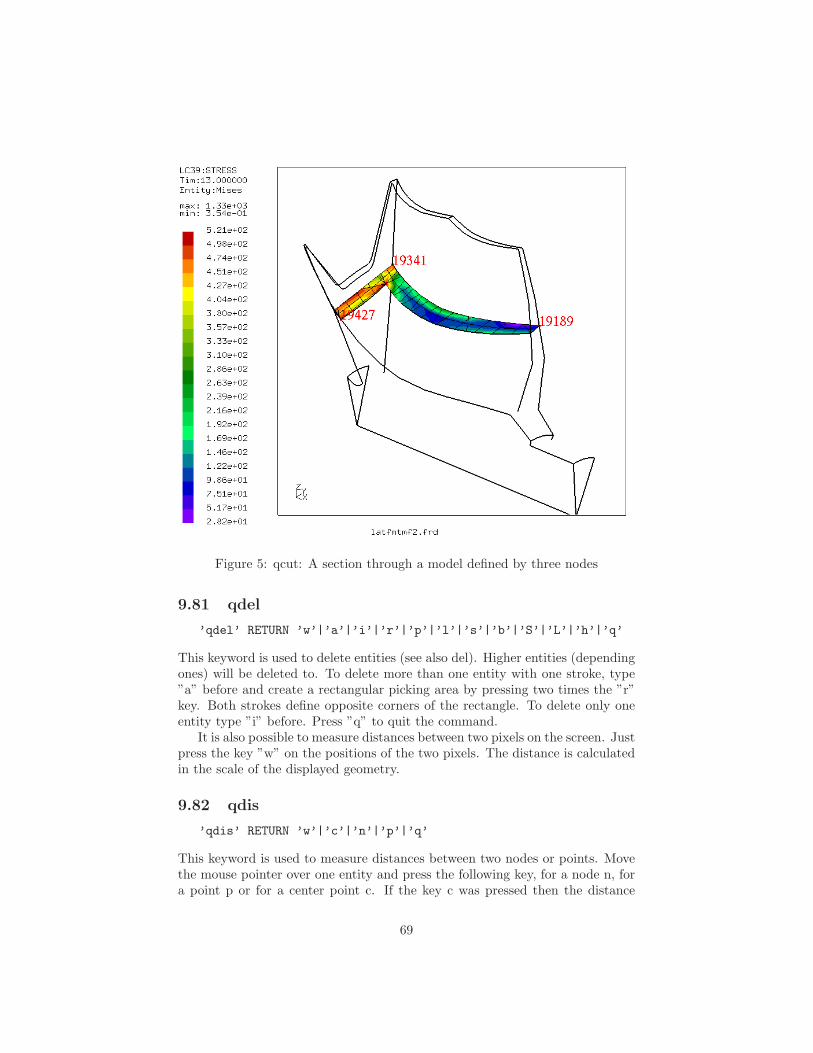
Figure 5: qcut: A section through a model defined by three nodes
9.81 qdel
’qdel’ RETURN ’w’|’a’|’i’|’r’|’p’|’l’|’s’|’b’|’S’|’L’|’h’|’q’
This keyword is used to delete entities (see also del). Higher entities (dependingones) will be deleted to. To delete more than one entity with one stroke, type”a” before and create a rectangular picking area by pressing two times the ”r”key. Both strokes define opposite corners of the rectangle. To delete only oneentity type ”i” before. Press ”q” to quit the command.
It is also possible to measure distances between two pixels on the screen. Justpress the key ”w” on the positions of the two pixels. The distance is calculatedin the scale of the displayed geometry.
9.82 qdis
’qdis’ RETURN ’w’|’c’|’n’|’p’|’q’
This keyword is used to measure distances between two nodes or points. Movethe mouse pointer over one entity and press the following key, for a node n, fora point p or for a center point c. If the key c was pressed then the distance
69
between the two nodes or points are given in cylindrical coordinates. Here lcir isthe length of the arc da the angle dr is r2-r1. If no center point was chosen thenthe distance and its xyz components are given in the Cartesian system. But inaddition the cylindrical distances around the origin and around the xyz-axis arealso given. Press ”q” to quit the command.
• dist: global distance
• dx, dy,dz: distance in the three Cartesian directions
• da: global angle
• dax, day, daz: angle around x, y, z
• dr: global radius difference
• drx, dry, drz: radius difference around x, y, z
It is also possible to measure distances between two pixels on the screen. Justpress the key ”w” on the positions of the two pixels. The distance is calculatedin the scale of the displayed geometry.
9.83 qdiv
’qdiv’ RETURN ’w’|’a’|’i’|’1’-’9’|’ 10’-’ 99’|’q’
This keyword is used to change the division of a line by pressing a numberbetween 1 and 9 when the mouse pointer is at the position of a line (see alsodiv). To define numbers between 10 and 99 press the space bar when the mousepointer is at the position of a line and then the number. To select more thanone line with one stroke, type ”a” before and create a rectangular picking areaby pressing two times the ”r” key. Both strokes define opposite corners ofthe rectangle. To select only one line type ”i” before. Press ”q” to quit thecommand. General rules are described in ”div”.
It is also possible to measure distances between two pixels on the screen. Justpress the key ”w” on the positions of the two pixels. The distance is calculatedin the scale of the displayed geometry.
9.84 qenq
’qenq’ RETURN ’w’|’a’|’i’|’r’|’n’|’e’|’f’|’p’|’l’|’s’|->
’b’|’S’|’L’|’h’|’m’|’u’|’v’|’t’|’q’
This keyword is used to gain information about entities. It is especially usefulto get the values on particular nodes.
If the maximum or minimum value in a certain area has to be searchedtype first “m” to go in the max/min mode and create a rectangular pickingarea by pressing two times the ”r” key. Both strokes define opposite corners ofthe selection-rectangle. Then the key “h” (high) to search the node with the
70

maximum value. The minimum is searched with “l” (low). The search-result isthen shown in the xterm and also attached to the node. With the “u” key thelast search result can be deleted (“undo”). The ’t’-key changes into the “qtxt”-mode. The ”qtxt” functionallity is now available which allows to manipulatethe node-attached-string and its position on the screen. Use ”qadd” instead of“qenq” if you need to save the node in a set for further use.
To catch more than one entity with one stroke, type ”a” (all) before andcreate a rectangular picking area by pressing two times the ”r” key. Bothstrokes define opposite corners of the rectangle. To catch only the entity whichis closest to the user type ”i” before.
Then move the mouse pointer over the entity(s) and press one of the followingkeys, for Nodes n, Elements e, Faces f, Points p, Lines l, Surfaces s, Bodies b,Nurb Surfaces S and for Nurb Lines L.
The position of nodes or points are given in Cartesian and cylindrical co-ordinates (see figure 6, axyz are the 3 angles around x,y and z, rxyz are the 3radii around x, y and z). In a second row the sets to which the picked entitybelongs are listed.
Press ”q” to quit the command.It is also possible to measure distances between two pixels on the screen. Just
press the key ”w” on the positions of the two pixels. The distance is calculatedin the scale of the displayed geometry.
Figure 6: qenq: Definition of the cylindrical system
71
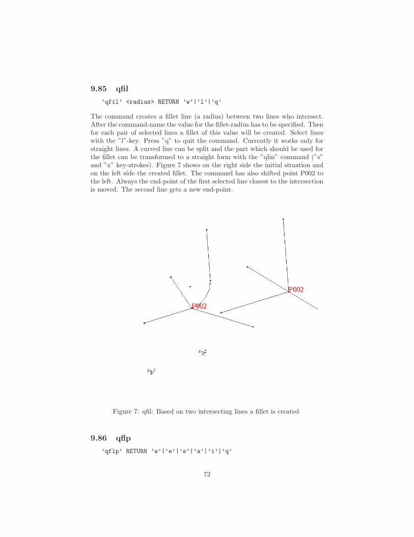
9.85 qfil
’qfil’ <radius> RETURN ’w’|’l’|’q’
The command creates a fillet line (a radius) between two lines who intersect.After the command-name the value for the fillet-radius has to be specified. Thenfor each pair of selected lines a fillet of this value will be created. Select lineswith the ”l”-key. Press ”q” to quit the command. Currently it works only forstraight lines. A curved line can be split and the part which should be used forthe fillet can be transformed to a straight form with the ”qlin” command (”s”and ”x” key-strokes). Figure 7 shows on the right side the initial situation andon the left side the created fillet. The command has also shifted point P002 tothe left. Always the end-point of the first selected line closest to the intersectionis moved. The second line gets a new end-point.
Figure 7: qfil: Based on two intersecting lines a fillet is created
9.86 qflp
’qflp’ RETURN ’w’|’e’|’s’|’a’|’i’|’q’
72
This keyword is used to invert the outer- and inner side (the orientation) ofshell-elements and surfaces. The orientation of shell-elements or surfaces can beseen by the interior color. The outer face reflects light, if the face is dark-greyit is the back-side. If ”Toggle Culling Back/Front” was selected before thenboth sides are illuminated. To flip the orientation of a surface and all relatedshell-elements select either a shell-element with the ”e” key or if the illuminatedsurfaces are displayed (see “rep” how to do that) select the surface with the”s” key. To see the effect on the elements immediatelly they must have beendisplayed with the ”plot” command. If only elements are in the database flipthem with the ”e” key. The ”a” key has a different meaning than usually. Ifpressed before a selection then a so called auto mode is activated. It makes sensefor volumes were a vector pointing in or out can be determined for all surfaces.In this case all related surfaces (and embedded elements) are oriented in thesame way as the selected one. It works only in situations were only two surfacesshare a common edge. This is the case for volumes without inner surfaces ora 2D model. In case of a volume all surface normals will point either inwardsor outwards, depending on the orientation of the selected surface. Press ”q” toquit the command.
It is also possible to measure distances between two pixels on the screen. Justpress the key ”w” on the positions of the two pixels. The distance is calculatedin the scale of the displayed geometry.
9.87 qint
’qint’ RETURN ’w’|’l’|’q’
This keyword is used to extend two lines to their intersecting location. Theend-points of the two lines are moved to the intersecting location but theyare not merged. Use the ”merg” command to merge duplicate points. Onlystraight lines are supported. Select lines with the ”l”-key. Press ”q” to quit thecommand.
9.88 qlin
’qlin’ <name>(optional) RETURN ’w’|’b’|’c’|’e’|’g’|’l’|’m’|’p’|->
’q’|’s’|’t’|’u’|’x’
This keyword is used to create a sequence of lines (or just one, see also line).The user might specify a name in the command-line or by picking an existingline with the key ”l”. In this case an existing line might be redefined withoutdestroying related geometries.
To start a sequence of lines move the mouse pointer over a point and pressthe key ”b” (begin).
To define just a straight line go to the end point and press ”g” (generate).This point is also the starting point for the next line. So no ”b” is necessary forthe next line.
73
If the line is a sequential line (spline) then the points of the sequence mustbe defined with the key ”t” in the correct order, but the last point must beselected with the key ”g”.
If the line is an arc then the center point must be selected with the ”c” keyor one point on the line between the end-points must be selected with the ”m”key, but the last point must be selected with the key ”g”.
In case you need to split a line during the process, you can do that bypressing the ”s” key.
When you want to modify the length then pick an existing line with the key”l” and then the endpoint you want to move with the key ”p”. The displacementis requested and the point is moved in the direction of the line by the specifieddisplacement.
The ”x” key will transform the line into a straight line.One quite usefull function for cad-based surfaces is triggered by the ”e”-
key (exchange). This allows to modify an existing surface (gsur). With thatcommand a line or a line sequence in a lcmb can be exchanged by the previousselected (“l” key) or generated line. For example one edge of an already existingsurface uses a lcmb but the user wants to replace it by a spline (line) then theuser defines or selects the new spline and then moves the mouse in an area wereone of the old lines (the new one might be present as well) is located and pressesthe ”e” key. The definition of the lcmb will be changed without destroying thesurface-definition.
Press ”q” to quit the command or ”u” to delete the last created line.It is also possible to measure distances between two pixels on the screen. Just
press the key ”w” on the positions of the two pixels. The distance is calculatedin the scale of the displayed geometry.
9.89 qmsh
’qmsh’ RETURN ’i’|’a’|’e’|’f’|’v’|’n’|’l’|’c’|’s’|’m’|’d’|’h’|’t’|’q’
A very usefull command to optimize surface meshes as a basis for tet-meshes.Line divisions can be changed by selecting a line with the “l” key and then anumber as for qdiv. The mesh will be updated automatically.
Based on identified lines “l” or surfaces “s” meshes can be coarsened ’t’,refined ’h’, deleted “d” and generated “m”. Surfaces can be combined “c” toget rid of very small ones and splitted ’b’.
To change the mesh density along a line:
• Identify a line or several lines with key “l”. The related surfaces areselected.
• The line division is changed by pressing the key with the desired num-ber. This function of qmsh works like the “qdiv” command. The relatedsurfaces are automatically re-meshed.
74

Example for a surface combination:
• Identify a line with key “l”. The related surfaces are selected.
• Or identify two adjacent surfaces with key “s” or by selecting two singleelements “e” one for each surface. They must use the same lines at thejunction.
• To combine the two selected surfaces press key “c” (Attention: The sur-face with the longer perimeter must reference a shape (a nurbs)). In themoment an automatic adaption of the embedded shape or nurbs is notdone. The shape of the bigger surface is just used for the combined sur-face. It might be necessary to use a mapped mesh for the new surfaceif the embedded shape is too small ( use tr6 instead of tr6u, see elty ormshp).
A surface (only without holes!) can be splitted by a crossing line:
• First create the desired splitting line, for example with “qlin”.
• Type “qmsh” and identify the line with key “l”.
• Identify the surface with key “s” or by selecting a single element “e”.
• Press key “b” to break (split) the surface in two. The previously selectedline will be converted to a spline with as much control points as the linedivision. Then the line-points are projeted to the surface.
To change the mesh density in a selected surface:
• Select one or more surfaces with key “s” or by selecting lines “l” or byselecting a single element “e”.
• Press “h” (higher) to increase the mesh density or “t” (thinner) to de-crease.
•This keyword can be used to manually define elements. The key “n” selects
nodes and the key “f” or “v” generate a surface or volume element based on thenode-selection.
To catch more than one entity with one stroke, type ”a” (all) at first. Thencreate a rectangular picking area by pressing two times the ”r” key. Both strokesdefine opposite corners of the selection-rectangle. To catch only the entity whichis closest to the user type ”i” before.
9.90 qnor
’qnor’ RETURN ’w’|’p’
A new line normal to a plane defined by three points and a length is created.It starts at the last point.
75

9.91 qpnt
’qpnt’ <name>(optional)RETURN ’w’|’p’|’g’|’m’|’n’|’s’|’S’|’u’
This keyword is used to create or move points (see also pnt). The user mightspecify a name in the command-line if a certain name should be used. Tocreate a point move the mouse pointer to the desired location and press thekey ”g” (generate) or over an existing node and press ”n” (uses then the node-coordinates). After a point was selected with ”p” it can be moved in differentways: Either in the screen-plane, for this go to the desired position and press”m” (move, see qali or the section Orientation how to rotate the model into acertain position). Or the point can be moved to the position of a second point,for this go to the second point which coordinates should be used and press ”p”again. If the coordinates of a node should be used press ”n” instead. Also anormal projection to a nurbs related surface (from cad-systems) is feasible bychoosing the target-surface with the ”s” key or a NURBS-surface with the ”S”key either before or after the point was marked. Press ”q” to quit the commandor ”u” to undo the last action.
If you picked the wrong point (the one which should be moved), just pickthe same again and pick then the correct one.
It is also possible to measure distances between two pixels on the screen. Justpress the key ”w” on the positions of the two pixels. The distance is calculatedin the scale of the displayed geometry.
9.92 qnod
’qnod’ RETURN ’w’|’p’|’m’|’u’
This keyword is used to move nodes (see also node). To move a node move themouse pointer to the desired node and press ”p” (pick) then go to the desiredposition and press ”m” (move). See qali or the section Orientation how to rotatethe model into a certain position. Press ”q” to quit the command or ”u” toundo the last action.
It is also possible to measure distances between two pixels on the screen. Justpress the key ”w” on the positions of the two pixels. The distance is calculatedin the scale of the displayed geometry.
9.93 qrem
’qrem’ <set> RETURN ’w’|’a’|’i’|’r’|’n’|’e’|’f’|’p’|’l’|’s’|->
’b’|’q’
This keyword is used to erase entities from a set (see also setr). To removeentities move the mouse pointer over the entity and press the following keys,for Nodes n, Elements e, Faces f, Points p, Lines l, Surfaces s, Bodies b, NurbSurfaces S and for Nurb Lines L. To catch more than one entity with one stroketype ”a” before and create a rectangular picking area by pressing two times the
76
”r” key. Both strokes define opposite corners of the rectangle. To catch onlyone entity type ”i” before. Press ”q” to quit the command.
It is also possible to measure distances between two pixels on the screen. Justpress the key ”w” on the positions of the two pixels. The distance is calculatedin the scale of the displayed geometry.
9.94 qseq
’qseq’ [<set> RETURN ’n’|’p’]|[ RETURN ’nr’]
This keyword is used to define a sequence. The sequence might consist of nodesor points. A sequence is nothing else than a set which keeps the selection-orderof the entities:
qseq nodeset
will store all selected nodes (selected with the ’n’ key) in the order in whichthey were selected. This set might be used for a subsequent ”graph” command.Point sequences are used to define splines. If
qseq
is typed without a setname then an existing line has to be selected with anumerical keystroke (or the space-bar followed by two numbers). New pointswill be created on this line which in turn are used to redefine the selected lineas a sequence-line which uses the new spline-points. Sequences can be shownwith the “prnt sq” command. Node sequences can be written to a file and readagain with the commands “send seqname fbd” and “read seqname.fbd”.
9.95 qshp
’qshp’ RETURN ’w’|’n’|’p’|’g’|’h’|’s’|’S’|’c’|’q’
This keyword is used to define a plane shape. A plane shape needs 3 points (ornodes, points at their location will be generated and used) for its definition. Thepoints are selected with the ’p’ (nodes ’n’) key. After the points are selected itwill be generated by a ’g’ keystroke. The shape can be assigned to a surface byselecting first either a shape ’h’ or a nurbs ’S’ and then the surface with the ’s’key. The shape will then define the interiour of this surface. The selected shapeor nurbs stay selected until cleared with ’c’. See also “shpe” for the keyboardcontrolled definition of shapes.
It can also be used for projection purposes (see ”proj”) or splitting (see”split”).
9.96 qspl
’qspl’ RETURN ’w’|’s’|’q’
77
This keyword is used to split one or more lines at a certain position (can alsobe done with ”qlin”). A point is created at the splitting position, the originalline is deleted and two new lines will appear instead. All lines running throughthe selected location will be split at once and the newly created splitting pointswill be merged to one if they are closer to each other than defined by ”gtol”. Tosplit a line move the mouse pointer over the line and press the ”s” key. Press”q” to quit the command.
It is also possible to measure distances between two pixels on the screen. Justpress the key ”w” on the positions of the two pixels. The distance is calculatedin the scale of the displayed geometry.
9.97 qsur
’qsur’ <name>(optional) RETURN
’w’|’a’|’b’|’l’|’i’|’r’|’1’-’9’|’g’|’q’|’u’|’s’|’S’|’h’|’c’
This keyword is used to create or change a surface (see also gsur). The usermight specify a name in the command-line or by picking an existing surfacewith the ”s” key.
If the surface is supposed to be meshed with unstructured triangles (elementtype tr3u or tr6u) it is sufficient to select all lines with the “l” key (lowercase“L”). This can be done either in the “all”-mode (press “a”) or “individual”-mode(press “i”) which is default. Then generate the surface by pressing the ”g” key.Such surfaces allow holes in it. If the surface is not plane it will need to referencean embedded NURBS surface (see ”nurs”) or a shape (see ”shpe”). Despite itis quite an exception it should be noted here that this kind of mesh might beextruded in the 3rd dimension by using the ”swep” command to generate pentaelements for the cfd solver.
For the definition of a regular meshable surface three to five edges must bedefined. To create a surface move the mouse pointer over the first line of thefirst edge and select it with the ”1” key (number “one”). If more than one lineis necessary to define the first edge select the following ones one after the otherwith the ”1” key. Each marked line is listed in the mother xterm. If all linesof the first edge are selected select the lines of the second edge by pressing the”2” key, then the third and eventually the fourth and fifth. The last selectedline must match the first. All lines defining an edge will create a combined line(see lcmb) and this combined line will show up in the definition of the surface.Then generate the surface by pressing the ”g” key and you might continue withthe next surface. By default the interior of the surface is defined according toCoons [13] which is a blended function. But it can also follow an embeddedNURBS-surface or a shape. To relate a surface to an existing NURBS surfaceselect another surface which already uses the desired NURBS with the ”S” key(uppercase) or to reference the shape with the “h” key. Then select the target-surface with “s”. The target surface is converted to a NURBS surface whichis necessary to be meshable with unstructured triangles (tr3u, tr6u) and to beused to generate tet elements. The selected shape or nurbs will stay selected
78
until cleared with ’c’. In case the NURBS or shape in question is not related toa surface it is necessary to use ”qshp” to select first the NURBS or shape andthen the surface which should reference them.
An existing surface might be completly redefined without destroying thedefinition of related bodies or other geometries. After selecting a surface withthe “s” key the referenced lines might be replaced by selecting new ones. Theprevious selected lines are not longer referenced.
Replace assignments by the blended function with the ”b” key. To quit thecommand use the ”q” key or use ”u” to undo the last action.
It is also possible to measure distances between two pixels on the screen. Justpress the key ”w” on the positions of the two pixels. The distance is calculatedin the scale of the displayed geometry.
9.98 qtxt
’qtxt’ RETURN ’g’|’a’|’i’|’b’|’p’|’m’|’n’|’v’|’f’|’d’|’q’
This keyword is used to move node-attached texts (showing node-number andvalue, see figure 8) at certain positions in the drawing area or to manipulatethem otherwhise. They are created with the key “g” while the mouse-pointer isover the node to which it should be attached. Attention: They are only visibleafter the command ”plus nt all” was used (but they are immediatelly visiblewhen the the commands ”qenq” or ”qadd” were used instead of “qtxt”). Tomove a text pick it at the lower-left corner with the key ’p’ and place it withthe key ’m’ in the new location. To move it back to its node use ’b’. Deletethem with ’d’. The node-nr and the value in the text can be switched on and offwith the ’n’ and ’v’ key. The ’f’ key will toggle the format of the value between“int”, “float” and “exponent”. See the command ”font” on how to change thefont-size. See “txt” for the batch mode command
To catch more than one entity with one stroke, type ’a’ (all) before andcreate a rectangular picking area by pressing two times the ’r’ key. Both strokesdefine opposite corners of the rectangle. To catch only the entity which is closestto the user type ’i’ before.
9.99 quit
’quit’
This keyword is used to terminate the program without save.
9.100 read
’read’ [<geo-file> [’add’]]|
[<ccx-file> ’inp’ [’add’|’ext’|’nom’|’new’]]|
[<openFoam-file> ’foam’ [’add’|’ext’|’nom’]]|
[<result-file(frd)> [’add’|’ext’|’nom’]|[<setname>]]|
[<stl-file> [’add’|’ext’|’nom’]]|
79

Figure 8: qtxt: Node attached texts at two locations, one with node-nr andvalue in exp-form and one just with his value in floating point form. The fontwith gives biggest numbers was used.
[<list-file> ’-n’|’-e’<column>]|
[<edge-file> ’edg’]|
[<netgen-file> ’ng’ [’add’|’ext’|’nom’|’ndsb’]]|
[<pixel-file> [<zoom>]|[<x_zoom> <y_zoom>]]
This keyword is used to read files or commands from a file. Most commandscan be read from a file but not all of them. In general all basic commands tocreate geometry are understood and up to now this is the only way to read predefined geometry during run-time. To read commands from a file like pnt, line,node, or seta and so on, type
read geo-file
this will eventually replace entities if their names were already in use. To pre-vent this, type
80

read geo-file add
this forces the program to change the names which are already in use to unusedones. Therefore no existing geometry will be overwritten.
If an ccx-input-file with loads, boundary-conditions and sets is read with acommand like
read ccx-file inp
then the loads and boundary-conditions are stored in automatically createdsets which start with a leading ’+’. For example the ccx command ’*BOUND-ARY’ will trigger the creation of the set ’+bou’. The ccx sets are stored in cgxsets of the same name. The load-values are stored in Datasets.
The option “nom” (no-mesh) can be used to speed up the reading of frd orinp formatted files like:
read ccx-file inp nom
and/or
read result-file nom
This option suppresses the reading of nodes and elements and makes sense ifthe mesh exists and only the set-definitions and loads or results should be read.
If the parameter ”add” is used,
read ccx-file inp add
then existing node- or element-numbers are not overwritten and the programchoses new numbers. If the ccx-input-file ends with “.inp” the parameter “inp”might be omitted.
An openFoam file [8] can be read in a similar way
read CaseDirName foam
as an ccx input file. Sets will be created if defined in the openFoam file. Resultscan be used for mapping purposes. For further details see “How to map loads”in the appendix.
The user might read a result-file in frd format during runtime. If a meshexists and should not be overwritten just add the parameter “add”
read result-file add
this forces the program to change the numbers which are already in use tounused ones. Existing datasets will be extended by the new node-numbers andtheir data. The option “ext”
81
read result-file ext
will also extend the existing datasets but in this case the nodes and elements areupdated (modified). If no parameter follows then existing nodes and elementsare updated and the new datasets will be appended to existing ones. Sincethe dependency checks are time consuming the user might scip them by usingthe ’ne’ parameter. Then the existing mesh is deleted before the new one is read:
read result-file new
It is also possible to read files written in the result format (.frd) during run-time only to define sets of nodes or elements without changing the definitionsof them. The command
read result-file setname
will create a set of the name setname and all nodes and elements listed inthe file mesh.frd will be added to that set. But this will NOT create or modifythe nodes and elements. All nodes and elements must exist and will not bechanged.
An stl file can be read with
read file.stl
.If a file with the numbers of nodes or elements is not available in the result
format (.frd) then a so called list-file could be read instead. In such a file eithernumbers of nodes or elements can be defined. The numbers found in a spec-ified column is interpreted as a node- or element-number. If ”-n” is specifiedthe numbers are interpreted as nodes and if ”-e” is specified the numbers areinterpreted as elements. For example
read list-file -e3
will define a set storing names of elements from the third column of file list-file.txt. The created set-name is always the name of the file.
NETGEN Import
In case NETGEN is used for meshing then the edges which are generated byNETGEN can be included for modifications;
read edge-file edg
82

will create beam elements based on the defined edges. When the modificationsare done, the beam elements can be exported in the NETGEN-edge formatwith the ”send setname stl” command and used for meshing in netgen (see also”How to deal with cad-geometry”). The netgen mesh can be imported with
read netgen-file ng
If the NETGEN (.vol) file contains solid elements, all shells and beams are onlyused to define surface sets of nodes and faces (+set<nr>). The shell elementsand beams are deleted by default. If you want to be more selective about theelements imported from netgen, you use the keyword ndsb (NoDeleteShellsAnd-Beams).
read myfile.vol ng ndsb
This keyword forces all the netgen elements to be imported. Be aware that theimported NETGEN element types (1D, 2D and 3D elements) are distributed invarious sets for further operations (as well as being contained in set ’all’). Forinstance the set ’+typ11’ will contain all elements of type 11 (2-node beams).Please see ”Element Types” for a key to the element numbers.
If a pixel-file in xwd-format is available it can be included as a background-picture. The user can then create geometry based on this picture:
read pixelfile 2 4
here the picture will be scaled by a factor of “2” in x- and “4” in y-direction.Delete it with ”del pic”. The picture can not be modified in cgx. Only scal-ing during reading (with either a global factor or separate scaling in x- andy-direction) is supported. Other modifications have to be made with externalsoftware.
The command parameters are writen to the ”stack”.
9.101 rep
’rep’ <set>
This keyword is used to refresh entities of a certain set. This is done automati-cally but with one exception: The rendering of the interior definition of surfacesmust be triggered manually with this command. The rendered surfaces can bedisplayed with ”plot” or ”plus” using the type ”si”.
9.102 rnam
’rnam’ <set> <set>
This keyword is used to rename a set.
83
9.103 rot
’rot’ [’u’|’d’|’r’|’l’|’c’ <angle>]|
[’x’|’-x’|’y’|’-y’|’z’|’-z’]
This keyword is used to rotate the view-direction to the model. For example
rot u 10
will rotate the view-direction 10 degrees upwards. The meaning of the otherletters is down d, right r, left l, clockwise c. The remaining letters will rotate theview into a pre-defined direction. For example the user will look in x directionafter the command
rot x
and against the x direction with the command
rot -x
and so on.
9.104 save
’save’
This keyword is used to save the geometry (if any) to a file named as the inputfile but with the extension .fbd. If a file with that name exists already, thenthis file will be saved with the new file extension .fbb as a backup.
9.105 scal
’scal’ [’s’|’v’|’d’] [<value>]
This keyword is used to scale the graphic presentation of values but no valuesof entities. The scaling of the value itself can be done with the command ”ds”.For example the command
scal s 0.5
will scale the range of values presented in the color plot by a factor of 0.5.The command
scal v 5.
will scale the length of vectors by a factor of 5. The command
84

scal d 2.
will scale the deformed shape by a factor of 2. Without a value it restoresthe default value. See also ”Toggle Vector-Plot”, ”Toggle Add-Displacement”,”Datasets”.
9.106 send
’send’ ’init’|
<set> ’fbd’ [’c’,’e’]| ->
’stl’| ->
’abq’|’ans’|’ast’|’dar’|’duns’|’frd’|’gmp’|->
’lst’|’nas’|’ng’|’pat’|’tcg’ <RETURN>|
[’bin’]|
[’ds’<nr>[+] [e<nr>[’,’|’-’<nr>]..]]|
[’tmf’]|
[’sta’ <refspeed>]|
[’crp’ <timefact> <refspeed> <writefreq>]|
[’comp’]|
[’mpc’ [[<rotation>|’v’<node> <v1> <v2> <v3> ]|
[’n’<node>]]]|
[’names’]|
[’spc’ <dofs(1-6|t|p)> <value>]| ->
[<dofs(1-6|t|p)> ’ds’<nr> e<nr>]| ->
[’nor’ <fac1> [<fac2> <fac3>]]| ->
[’nor’ ’ds’<nr> ’e’<nr>]|
[’spcf’ <dofs(1-6|t|p)> <value>]| ->
[<dofs(1-6|t|p)> ’ds’<nr> ’e’<nr>]| ->
[’slide’ ’c’|’s’|’rx’| ->
’ry’|’rz’|’tx’|’ty’|’tz’]|
[’pres’ [<value>]|[’ds’<nr> ’e’<nr>] [+|-] ]|
[’film’ [[n<nodnr>][<temp>]|->
[[[’ds’<nr>]|[sq<dsnr>-<dsnr>]] ’e’<nr>]->
[[<coeff>]|->
[[’ds’<nr>]|[sq<dsnr>-<dsnr>] ’e’<nr>]] [+|-] ]|
[’rad’ [[<temp>|[cr<temp>]|[’ds’<nr> ’e’<nr>]] ->
[[<emis>|[’ds’<nr> ’e’<nr>]] [+|-] ]|
[’dflux’ [[<load>]|[’ds’<nr> ’e’<nr>]] [+|-] ]|
[’mflow’ [[<load>]|[’ds’<nr> ’e’<nr>]] [+|-] ]|
[’cflux’ <load>]|
[’force’ <f1> <f2> <f3>]|
[’quadlin’]|
[’sur’ [+|-] ]
’send’ <set> [’dolfyn’|’duns’|’isaac’|’foam’] [<type> <set>] | ->
[’cyclic’ <set> <set> ’tx’|’ty’|’tz’|’rx’|’ry’|’rz’|
’cx’|’cy’|’cz’|<vx,vy,vz>]
85
’send’ <dep-set> <indep-set> ’nas’|’abq’|’ans’ [’cycmpc’|’cycmpcf’ ->
’px’|’py’|’pz’|’tx’|’ty’|’tz’| ->
’rx’|’ry’|’rz’|’cx’|’cy’|’cz’<+-segments> ’c’|’u’<NR>]| ->
[’areampc’ <dofs(’t’|’p’|’1-6’)> ’c’|’u’<Nr>]|’f’<value> ->
[’areampc’ ’slide’]| ->
[’areampc’ ’presfit’ [’s’<value>]]| ->
[’gap’ <vx> <vy> <vz> <tol>]
This keyword is used to send data to the file-system. In certain cases the writtenfile-name contains given parameters to make them unique which is convenientwhen the user writes several files of the same type. But on the other handthis makes it sometimes hard to know in advance how the file would be named.Therefore the send command writes the file-name to the stack from which theuser can derive the name if the ”stack” was activated.
The following formats are known (but not all options for all formats are fullysupported so far); The geometry-format (fbd)
send set fbd
or
send set fbd c
will complete the set downwards before writing, or
send set fbd e
will write all model-edges as small lines running from node to node. A spe-cial case of a command file is written with
send init
named init.fbl which stores status variables (also written at the end of geometryfiles). This can be used in a second or later session by reading it with the ”read”command:
read init.fbl
The user might use the ”menu” command to define two command lines forthe writing and reading of the init file to a certain location. With this approacha certain orientation of the model can be quickly stored and restored.
A surface description with triangles (stl)can be written:
send all stl
This triangles are based on elements which were created by meshing surfaces or
86

by automatically triangulated element-faces of all types of supported elements.If be2 elements are included in the mesh (meshed lines) a so called edge filefor NETGEN will also be created if stl is written. NETGEN provides also astand-alone mesher called ng vol. The mesher can be found in the netgen sub-directory nglib. As for the stl-format triangles can be written for this mesherwith:
send set ng
It has the advantage that the triangles are directly used to define tetras and notas with stl are only used to define the outer shape of the body.
The following mesh-related formats are known: Femview and CADfix (frd),Nastran (nas), Abaqus (abq), Ansys (ans), CodeAster (ast), Samcef (sam), Dar-win (dar), patran (pat, only sets), gagemap (gmp, only sets) and Tochnog (tcg)but only ccx (Abaqus) is fully supported. Good support is also provided foransys, darwin and nastran. If no further parameter follows then just the defini-tion of the nodes and elements will be written:
send all abq
will write the mesh in the format used by Abaqus and the CalculiX solver.If the parameter ”ds” is provided followed by the dataset-nr
send set abq ds1
then the values stored in Dataset 1 are written. For ’frd’-format the ’ds’ pa-rameter w/o any further values forces cgx to write all datasets but w/o theinternally calculated ones:
send all frd ds
If a “+” sign appears at the end of the ’ds’ parameter
send all frd ds+
or
send all frd ds1+
then also the internally calculated values like vMises-stress are written. Ad-ditionally the entities might be specified with the ’e’ parameter followed by thenumbers to write. The numbers have to be separated by a ’,’ sign or in case ofa range by a ’-’ sign:
send all frd ds1 e9,25-30
87

The “bin” parameter has the same meaning as the “ds” parameter but inthis case the result is written in the binary form of the frd-format (alwaysall datasets). In case data should be written for the crack analysis tool Darwin
send all dar ds
will write all datasets. Since Darwin changed the format from version 7.1 on, itis possible to change the format with the parameter ’v7.1’ as the last parameter.If the set is of the ordered type and includes nodes (see “qseq”) then the dataare written in tabular form for use in a 1D crack-prop Darwin-analysis.
In certain circumstances the user needs an easy solver independent formatto write node- and element numbers. This is provided by the “lst” parameter:
send setname lst
will write the node- and element-numbers in lines of seven space separatedrows.
Missing lower entities (nodes, points, lines etc.) will be added to the set be-fore the set is written if the parameter ”comp” follows. For example geometrylike bodies
send set fbd comp
will be extended by surfaces, lines and points or
send set frd comp
will include all nodes used by the elements to the set elem and will then writethe file.
The parameter “quadlin” forces the conversion from second order elements intosingle order elements were each element is subdivided into 8 single order ele-ments. This takes place during writing and will not change the current state ofthe mesh in cgx. Up to now it is only available for the abq format:
send all abq quadlin
If the parameter ”tmf” follows the definition of a solver format
send set abq tmf
then the mesh plus all temperatures with the necessary solver context for tmfcalculations is written. If the parameter ”sta” follows
send set abq sta 2900.
88
then the mesh plus all temperatures with the necessary solver context for astatic calculations is written. Here the value for ”speed” is a reference valuefor eventual numerical values in the TEXT-Block of the Datasets in the resultfile (frd-file, see ”Nodal Results Block”). A scaling factor will be determinedbased on the reference value (here a ref.speed of 2900.) and the individualTEXT-Block values (factor = speed**2 / refspeed**2). This factor is used in*AMPLITUDE commands which will also be written and will be used to scalestatic loads which are referenced in the *STEP data. If the parameter ”crp”follows
send set abq crp 1. 2900. 1
then the mesh plus all temperatures with the necessary solver context for creepcalculations is written. Here the value for ”timefact” scales the time-values ofthe Datasets, ”speed” is a reference value for scaling static loads (see option“sta”) and writefreq limits the output to the result-file.
If the parameter ”names” follows the solver-type then just the element- or node-numbers are written. This is useful for defining sets for the solvers. The com-mand
send steel abq names
will write the node and element numbers included in ”steel”. This file couldbe used to define a set for material assignments, boundary conditions or loads.If all sets should be written at once, use:
send all abq nam
If the solver-format ”duns” is used then related numbers of surfaces (3D) orlines (2D) will be written. This information is necessary to apply boundary-conditions to duns. The numbers are used in the connectivity file (duns.conn)which will be created by the mesh-command. The user has to refer this numbersin the duns.script2 file when assigning boundary conditions.
It is also possible to define and send some constraints to the file system. Toconstrain degrees of freedom (dof) of selected nodes use the parameter ”spc” incombination with the numbers of the constrained dofs and optionally a forceddeflection. For example:
send hinge abq spc 123
will constrain the translational degrees of freedom of the nodes in set ”hinge”.Or
send hinge abq spc 12356
89

will leave just one rotational degree of freedom unconstrained. And
send move-nodes abq spc 1 0.1
will move the nodes in set move-nodes by 0.1 in direction 1.
send move-nodes abq spc 1 ds1 e1
will use the values from dataset-nr 1 and the entity-nr 1 for the forced dis-placement in direction 1 and
send move-nodes abq spc nor 0.1
will force the nodes included in set move-nodes by 0.1 in the normal direc-tion (normal to the element-faces). The components of the vectors at the nodepositions can be scaled individually (fac1-3)). The vector length can also beread from an entity of a dataset:
send move-nodes abq spc nor ds1 e4
A subsequent calculation with ccx will move the mesh accordingly. After solvingthe deformed mesh can be used as a new mesh for further calculations. With thisprocedure geometric variations are possible without manipulating the geometry(morphing).
For cfd there is a “spc” function available which works on faces instead onnodes (see *BOUNDARYF in the ccx manual).
send Inlet abq spcf 123
The degees of freedom 123 define velocities and not deflections. Its called “spcf”and works otherwhise accordingly to the “spc” command.
The parameter ”slide” in combination with one additional parameter willcreate equations that force the selected nodes to move only in a plane. If theadditional parameter ”s” is specified then the specified nodes will be attached totheir element faces. All nodes of the affected element-faces have to be selected.For example you type:
send sur abq slide s
and this should attach the node with the node-nr. 1 to a plane parallel tothe surface of the corresponding element-face. This element uses the node 1,2, 3, 4, 5, 6, 7 and 8 where 1, 2, 3 and 4 are on the surface of the mesh. Theprogram will detect this element face and constrain the node only then if thenodes 2, 3 and 4 were also included in the set ”sur”! The detected elements orfaces of volume-elements will be assigned to the set. So it is possible to checkthe detected elements. Instead of providing a set with the necessary nodes, you
90
might instead provide a set with shell-elements or/and faces of volume-elements.The nodes will be derived from them. In most cases this is the most convenientway.
A special case which works probably only in ccx (abaqus might give wrongresults) is triggered by the “c” parameter. It behaves as for the “s” parameterbut works for cycsym calcs:
send cycsur abq slide c
A new set with new nodes will be created with the name “<set> COPY” whichhas to be used in the cycsym definition in ccx instead of “<set>”. In addi-tion equations are specified which connect the new nodes with the original onesin the normal direction of the element faces. In this way two faces used in acyclic symmetry connection will slide at each other instead of beeing glued inall directions.
If nodes should slide radially to the y axis then use ”ry”:
send sur abq slide ry
or use ”ty” if the nodes should move only tangential to the y axis. In bothcases the axial movement is still permitted.
The parameter ”sur” will write the surfaces of the mesh either in abaqus-format for the *SURFACE command or in frd-format as shell elements. Forexample
send top abq sur
will write the elements in set top together with the face-nr (Important: Onlyfree surfaces of the mesh are regarded, internal faces are unknown and can notbe identified). The front- or rear side of the face (pos or neg) is selected withthe ’+’ or ’-’ parameter:
send surset abq sur -
will write all surfaces in set surset in abaqus format but all surfaces whichhave a potentially negative side will be written in that manner.
The parameter ”pres” is used to assign pressure values to element faces. Forexample
send surf abq pres 0.05
will assign the pressure value 0.05 to all element-faces in set surf. If a datasetwith nodal values is available it is also possible to use this values instead ofusing a uniform value for all faces. For example
send surf abq pres lc1 e1
91

will specify the dataset-nr 1 and the entity-nr 1 to be used instead of a uni-form value. The front- or rear side of the face (pos or neg) is selected with the’+’ or ’-’ parameter (it has to be the last parameter).
The parameter ”film” is used to assign free-stream temperatures and ther-mal heat coefficients to element faces. It works similar to the ”pres” option.For example
send surf abq film 1200. 0.5
will assign the film temperature of 1200 and the coefficient 0.5 to all element-faces in set surf. If datasets with nodal values are available it is also possible touse this values instead of using a uniform value for all faces. For example
send surf abq film ds1 e1 0.5
will specify the dataset-nr 1 and the entity-nr 1 to be used for the tempera-ture instead of a uniform value, or
send surf abq film ds1 e1 lc1 e2
will specify also the dataset-nr 1 with the entity-nr 2 to be used for the film-coefficients instead of a uniform value. The front- or rear side of the face (pos orneg) is selected with the ’+’ or ’-’ parameter (it has to be the last parameter).Instead of a single dataset-nr a range can be given:
send surf abq film sq1-9 e1 sq1-9 e2
and instead of giving e determined value for the temperature a node of a ther-mal network can be specified with:
send surf abq film n1277 ds1 e1
The parameter ”rad” is used to assign a sink temperatures and the emissiv-ity to element faces. It works similar to the ”pres” option. For example
send surf abq rad 1200. 0.5
will assign the sink temperature of 1200 and the emissivity 0.5 to all element-faces in set surf. If datasets with nodal values are available it is also possible touse this values instead of using a uniform value for all faces. For example
send surf abq rad lc1 e1 1200.
will specify the dataset-nr 1 and the entity-nr 1 to be used for the tempera-
92

ture instead of a uniform value, or
send surf abq rad lc1 e1 lc1 e2
will specify also the dataset-nr 1 with the entity-nr 2 to be used for the emis-sivity instead of a uniform value. The front- or rear side of the face (pos orneg) is selected with the ’+’ or ’-’ parameter (it has to be the last parameter).If cavity radiation should be used then the command has to use the ’cr’ attribute:
send surf abq rad cr1000. 0.7
Here 1000. is either the sink temperature, or, if the ccx parameter ENVNODEis active (*RADIATE,ENVNODE), the sink node.
The parameters ”dflux” and ”mflow” are used to assign an energy streamor a mass-flow to element faces. They work similar to the ”pres” option. Forexample
send surf abq dflux 0.5
will assign the flux of 0.5 to all element-faces in set surf. And
send surf abq mflow 0.5
will assign the mass-flow of 0.5 to all element-faces of the given set. If a datasetwith nodal values is available it is also possible to use this values instead ofusing a uniform value for all faces. For example
send surf abq dflux lc1 e1
will specify the dataset-nr 1 and the entity-nr 1 to be used instead of a uni-form value. The front- or rear side of the face (pos or neg) is selected with the’+’ or ’-’ parameter (it has to be the last parameter).
The parameter ”cflux” is used to assign an energy stream to nodes. Forexample
send surf abq cflux 0.5
will assign the flux of 0.5 to all nodes in set surf.The parameter ”force” is used to assign force values to nodes. For example
send nodes abq force 1. 20. 0.
will assign the specified forces to all nodes of the set nodes.The parameter ”mpc” is either used to create input for the user-subroutine
umpc which forces all nodes from ”set” to rotate by an average value speci-fied with ”rotation” around the vector v, or to create a rigid body. In case of a
93

rotation the value has to be in degree were 90 degree is orthogonal. For example
send nodes abq mpc 4. 1. 0. 0.
will assign the nodes of the set ”nodes” to the user-subroutine umpc and willforce them to rotate by 4 degree around the x-axis. Two files are produced.The one with the equations has to be included in the model-definition-sectionand the boundary-file in the step section.
In case of a rigid-body request there are two other parameters in combina-tion with “mpc” available. The rotation value is replaced by a nodenr of anindependent node which will be created based on either provided coordinates
send nodes nas mpc v4711 1. 0. 0.
or by averaged coordinates based on the specified set (here “nodes”) whichare interpreted as dependent nodes:
send nodes nas mpc n4711
In both cases an RBE2 (nastran) or *RIGID BODY,REF NODE=nodenr (ccx,abq)element will be created which connect all this nodes. See also ”asgn” on how topredefine a thermal expansion coefficient “alfa” for this element (only nastran).
Another useful method are so called ”cyclic symmetry” equations. Theseequations are used when just a section of a rotation-symmetric part like a diskis modeled. These equations force the two cutting planes of such a section tomove exactly equal in the cylindrical system. If the coordinate system of thedisplacements for the solver is rectangular (xyz) then the syntax is:
send dep indep nas cycmpc rx12 c1
Here ”dep” is the set containing the nodes of the dependent side. These nodeswill be replaced by the solver with the independent nodes from the set ”in-dep”. In this case the equations will be written in the nastran format ”nas” (innastran called MPC). The parameter ”rx12” defines the displacement systemas rectangular ”r”, the rotational axis is ”x” and the ”12” defines the num-ber of segments in 360 deg, therefore the angle of the segment is 360 deg /12.Attention: The sign of the number-of-segments must be negative if the anglebetween the independent side and the dependent side is negative. When thenr-of-segments is omitted the value is calculated individual for each node. The”c” triggers the correction of the position of the dependent nodes to a positiondefined by the angle of the segment (highly recommended), ”u” would preventthe correction. The ”1” will be the identifier for the equations if the format isnas (nastran). In case the format would be ans (ansys) then the ”1” would bethe number of the first equation. No number is required for abq (abaqus and
94
calculix). If the coordinate system of the displacements is cylindrical (rtz) thenthe example would be:
send dep indep nas cycmpc cx12 c1
Only the ”r” from ”rx12” is changed to ”c”. A thermal connection is cre-ated with:
send dep indep nas cycmpc tx c
The thermal connection is triggered by the ”t”, a pressure connection with“p”. See comments above for the single parameters. In case of cfd elements thesyntax is similar but only the function name itself differs:
send dep indep abq cycmpcf rx12 c1
The function name for cfd elements is ’cycmpcf’ instead of ’cycmpc’.In addition it is possible to ”glue” independent meshes together. For this
purpose the dependent nodes are tied to independent elements by equations.Choose the finer mesh for the dependent side. The equations are based on theshape-functions of the element types. For example
send dep indep nas areampc 123 c1
will connect the nodes in the set dep to element-faces described by nodes in-cluded in the set indep. The set dep must contain all nodes which should be”glued” and the set indep should contain all nodes of the elements surfaces towhich the dep nodes should be glued. The numbers ”123” are the degrees offreedom which will be connected (”t” will create a thermal connection, “p” apressure connection). The ”c” triggers the correction of the position of the de-pendent nodes to a position on the surface of the independent elements (highlyrecommended and default), ”u” would prevent the correction, “f” forces thedependend node away from the independent face. Of course the mesh has tobe written after the use of such a command, otherwhise the corrected nodepositions would not be regarded and the equations would lead to increased stiff-ness and decreased accuracy. The ”1” will be the identifier for the equations ifthe format is nas (nastran). In case the format would be ans (ansys) then the”1” would be the number of the first equation. No number is required for abq(abaqus and calculix), see also ”How to connect independent meshes”.
There is also the ”slide” option in combination with the ”areampc” option:For example if the mesh of a turbine-blade and a disk should be connected witheach other in a simpler but realistic way then a sliding condition between thisparts can be established. The command:
send dep indep abq areampc slide
95
will connect the nodes in the set dep to element-faces described by nodes in-cluded in the set indep but only in the direction perpendicular to a plane definedby nodes of the dep-set. Therefore all dep-nodes and all indep-nodes must liein the same plane and will slide in the same plane!
Another case is considered with the ”presfit” option in combination withthe ”areampc” option. For example if a cylindrical press fit should be simulatedthen a forced displacement between the two intersecting surfaces is necessary.This forces the dependent nodes to move to the independent face. Two modesare available:
send dep indep abq areampc presfit f
simulates sticking friction and with the option s
send dep indep abq areampc presfit s
works for sliding conditions. The user might request a certain value for thepress fit if the overlapping of the mesh do not represent the necessary distance:
send dep indep abq areampc presfit s0.06
will move the dep-nodes 0.06 in the normal direction of the independent faces(works also with option f). Additional nodes are generated and can be usedto request the reaction forces on the dependent nodes. They are stored in aset named N¡dep-set-name¿¡ind-set-name¿. Two files are produced. The onewith the equations has to be included in the model-definition-section and theboundary-file in the step section.
Special cases are the cfd-solvers Duns, Isaac and OpenFoam. The boundarypatches are an integral part of the mesh. So it is necessary to specify all bound-ary patches when writing the mesh. All free surfaces of the mesh must bespecified. This is an example for OpenFoam:
send all foam cyclic cyc1 cyc2 cx patch in patch out wall wall
will write the so called polyMesh description to the file-system. After the sendcommand the set (all) with the mesh is specified, then the format (foam), thencyclic boundary conditions (cyclic cyc1 cyc2 cx) between set cyc1 and cyc2 ofthe axi-symmetric case around x (cx), then boundary conditions of type patchfor set ”in” (patch in), then boundary conditions of type patch for set ”out”(patch out) and boundary conditions of type wall for set ”wall” (wall wall).
The symmetric boundary-conditions (base-type: cyclic) can be axi-symmetric(c) around x,y,z or rectangular (r) in direction of x,y,z. Only for OpenFoam andin the rectangular (Cartesian) case also a vector pointing in the direction of thesymmetry can be specified (ie: 1.,1.,0.)
96
For dolfyn, duns and isaac the same syntax has to be used:
send all duns viscous-wall profil subsonic-inflow in subsonic-outflow out
send all isaac WALL profil FARFIELD far EXTRAPOLATE out
send all dolfyn INLE ingang OUTL uitgang ... etc
To define so called ”gap” elements and related control-commands: Theseelements will connect parts if they are closer as a certain distance. For exampleif the distance is zero (contact). The command:
send dep indep abq gap 1. 0. 0.
will connect the nodes in the set dep and indep with gap-elements but onlyif they match each other in the direction 1.
9.107 seqa
’seqa’ <seq> [’nod’|’pnt’ <name> .. <=>]|
[’afte’|’befo’ <name> ’nod’|’pnt’ <name>.. <=>]|
[’end’ ’nod’|’pnt’ <name> .. <=>]
This keyword is used to create or redefine a set marked as a sequential set.This set is used for spline definitions (see line). With the command qlin such asequential set is automatically created. To begin such a set type for example:
SEQA Q003 PNT P004 P005 P006 P00M P00N
The program will create or overwrite the set Q003. The command will con-tinue in the next line if the sign ”=” is found:
SEQA Q003 PNT P004 P005 P006 =P007 P008 P009
The parameter AFTE will insert additional points after the first specified pointin the existing sequence. The parameter BEFO will insert additional points be-fore the first specified point and the parameter END will add additional pointsto a sequence.
9.108 seqc
’seqc’ <set>
97

Converts an “lcmb into a spline. The lcmb will be deleted (not the referencedlines) and keeps the sum of divisions but sets the bias to 1.
9.109 seql
’seql’ <set> <nr>
Makes splines from all sorts of lines. The nr of new created inner points isdefined by the parameter nr. Also existing splines will be redefined.
9.110 seta
’seta’ <set> [’!’|’n’|’e’|’p’|’l’|’c’|’s’|’b’|’L’|’S’|’v’|’se’| ->
’sh’|’ld’<div> <[\]name|*chars* ..>] |
[’n’|’e’ <name> ’-’ <name> <steps>]
This keyword is used to create or redefine a set (see also qadd). All entities likepoints or bodies and so on must be stored at least in one set to be reachable.The set ”all” is created automatically at startup and will be open (see seto) allthe time unless explicitly closed (see setc). To add points to the set ”dummy”type:
seta dummy p p1 p2
This will add the points p1 and p2 to the set dummy. The following entities areknown:
Nodes n, Elements e, Faces f, Points p, Lines l, Surfaces s, Bodies b, NurbLines L, Nurb Surfaces S, Values v, names of other sets se or shapes sh. If theentity of the specified type does not exits a set of that name is assumed and ifexisting then all it’s entities of the specified type are appended:
seta set1 n set2
will append only the nodes in set2 to set1. If the type ’se’ is used then thefull content of set2 is appended. Wildcards (*) can be used to search for set-names of a certain expression.
The program will automatically determine the type of the entities if notspecified, but then the names must be unique. More than one name can bespecified. A minus sign between two numbers of nodes or elements specifies arange of entities with steps of ”steps”:
seta set1 n 1001 - 1100 12
If the ’ !’ sign is specified instead of a setname then the program generatesautomatically sets with system defined setnames and stores entities in it. This
98

can be used is to separate independent meshes and line-loops. The single inde-pendent meshes are then referenced by new setnames, for example:
seta ! all
will determine all separate (disjunct) meshes in set “all” and store them insets called +CF<nr>. Figure 9.110) illustrates this function. Other entitieshave to be specified as an additional argument after the ’ !’ sign:
seta ! l all
will determine all separate (disjunct) line-loops. Other entieties are not im-plemented so far.
Values ”valu” can be used as arguments. It is necessary to mask a valuewith a leading ’\’ In cases were the value should not be replaces by its content:
seta set v \val1 \val2
will not substitute the val1 and val2 but add the values itself to the set.Lines with a division higher than specified with
seta setname ld50
can be stored in a set. Here all lines with a division above 50 are stored insetname.
9.111 setc
’setc’ [<set>]
This keyword is used to close an open set. Without parameter setc will closethe at last opened set.
9.112 sete
’sete’ <set> ’n’|’e’|’p’|’l’|’c’|’s’|’b’|’S’|’L’|’se’|’sh’ ->
’max’|’min’|’strict’
This keyword is used to enquire other sets which have entities in common orwhich have an identical content. Example:
sete blade p min
searches for sets who store at least the same points as ”blade” (always theset ”all”). The option “max” searches for sets whose entities are completelyincluded in the specified set. The option “strict” searches for identical setsregarding the specified type of entity.
99
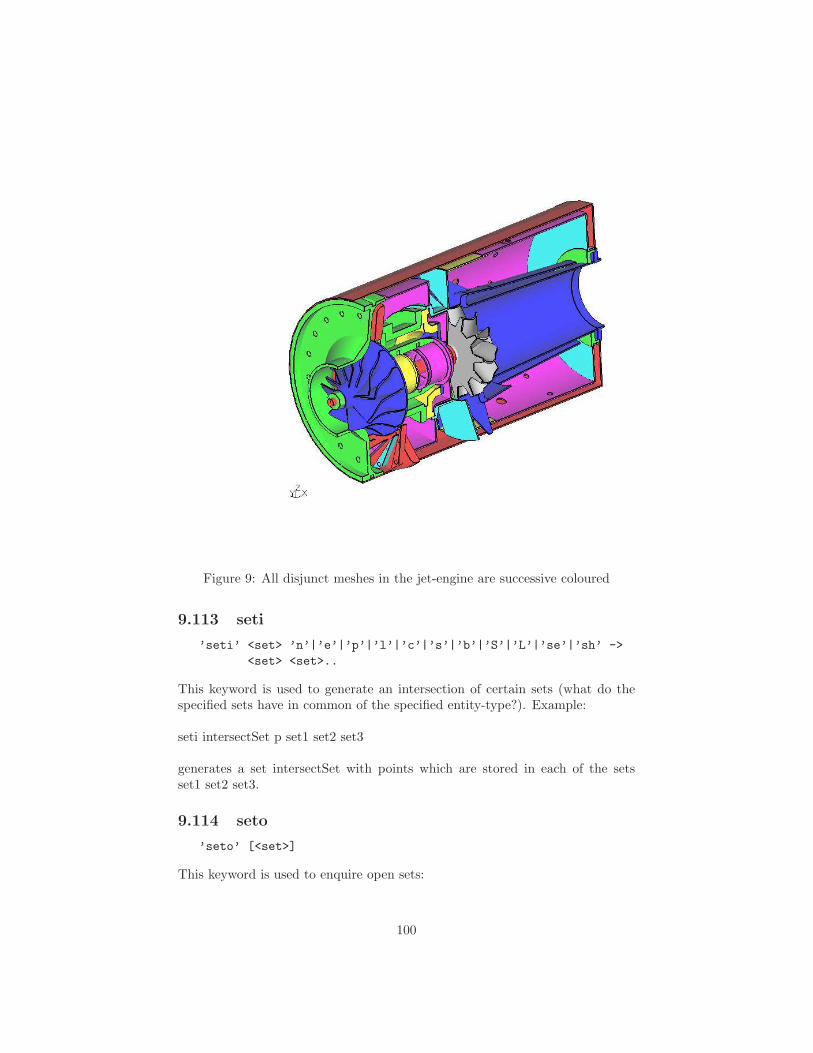
Figure 9: All disjunct meshes in the jet-engine are successive coloured
9.113 seti
’seti’ <set> ’n’|’e’|’p’|’l’|’c’|’s’|’b’|’S’|’L’|’se’|’sh’ ->
<set> <set>..
This keyword is used to generate an intersection of certain sets (what do thespecified sets have in common of the specified entity-type?). Example:
seti intersectSet p set1 set2 set3
generates a set intersectSet with points which are stored in each of the setsset1 set2 set3.
9.114 seto
’seto’ [<set>]
This keyword is used to enquire open sets:
100

seto
Or to mark a set as open:
seto set
All newly defined or redefined entities will be members of all open sets. Seesetc how to close an open set.
9.115 setr
’setr’ <set> ’n’|’e’|’p’|’l’|’s’|’b’|’L’|’S’|’v’|’se’|’sh’
<name|*chars*> <name|*chars*> ..
This keyword is used to remove entities from a set (see also qrem. The entitywill not be deleted. It is just not longer a member of that set. To remove entitiesfrom the set dummy type:
setr dummy p p1 p2
This will remove the points p1 and p2 from the set. The following entitiesare known: Nodes n, Elements e, Points p, Lines l, Surfaces s, Bodies b, NurbLines L, Nurb Surfaces S, Values v, other sets se and shapes sh. The programwill automatically determine the type of the entities if not specified, but thenthe names must be unique. Wildcards (*) can be used to search for setnamesof a certain expression.
9.116 shpe
’shpe’ <name|!> [’pln’ <P1> <P2> <P3>] |
[’cyl’ <P1> <P2> <R1>] |
[’con’ <P1> <P2> <R1> <R2>] |
[’tor’ <P1> <R1> <P2> <R2>] |
[’sph’] <P1> <R1>]
This keyword is used to create a shape which can be used to define the interiourof surfaces or to be used as a target for projections (see proj) or to split entities(see split). A plane shape is defined with the parameter “pln” followed by thenames of three points:
shpe H001 pln P1 P2 P3
A cylinder can be defined by
shpe H001 cyl P1 P2 10.5
101

were 10.5 is the radius. A cone can be defined by
shpe H001 con P1 P2 10.5 2.
were 10.5 is the radius at point P1 and 2. at point P2. A torus can be defined by
shpe H001 tor P1 10.5 P2 2.0
were 10.5 is the radius at point P1. Point P2 lies on the torus axis and 2.0is the radius of the tube. A sphere can be defined by
shpe H001 sph P1 10.5
were 10.5 is the radius at point P1. If automatic name generation is desired,then use ”!” instead of a name. See also “qshp” for the mouse controlled defi-nition of shapes. It should be mentioned that all shapes are actually nurbs andthat internally all nurbs which are used by surfaces are actually referenced bya shape as an interface.
Remark: A further shape type exists which links a nurbs to a surface defi-nition. Such a shape will be automatically generated when a nurbs is finishedby the “END” parameter using the same name as the nurbs. This shapes willnot be written to a file but using the prnt command will list them:
shpe N001 NURS N001
9.117 split
’split’ <set1> <set2>
This keyword is used to split lines, surfaces and elements.The split command will not generate new surfaces but it will create points
along the intersection between the surfaces in set1 and the surfaces (or shapesor faces) in set2.
So far only tetraeder elements (in set1) can be splitted by surfaces, faces orshapes (in set2). In this case the splitted tetraeder elements will be replaced bynew tetraeder- and pentaeder elements. It can be used to cut out parts of themesh to be either used directly in other models or which can be remeshed withtets based on an stl-file derived from them. Or it can be used to apply damagesto a structure. See “How to map loads” in the appendix on how to map loadsto the new created nodes from the original mesh.
9.118 stack
’stack’ on|off|free
Several functions which return values to the user might now place them also ona software-stack (used by area,dist,ds,enq,gtol,length,prnt,valu,volu and many
102

Figure 10: The shape types and its symbols together with an illustrating mesh
more). The “valu” command is able to read this values from the stack and placethem in variables. The ’free’ parameter will empty the stack but does not openor close it.
See also “if” and “while”.
9.119 steps
’steps’ <value>
This keyword is used to define the number of different colors in the post-processor mode. The default is 21.
9.120 surf
’surf’ <name(char<9)>|’!’ [<set>]|->
<line|lcmb> <line|lcmb> <line|lcmb> <line|lcmb>
This keyword is used to define or redefine a surface. It is a more convenient wayto define a surface than the command gsur. Either individual lines or a set oflines can be specified. To be meshable with structured elements it requires 3, 4
103
or 5 edges (lines or lcmbs). To be meshable with tr3u or tr6u it requires eitherto be plane or to reference a shape or nurbs which can not be provided with thiscommand (see “gsur” which allows the assignment of a shape or “qshp” whichallows the assignment of a shape or nurbs to a surface). The mouse controlledway to define surfaces is to use the command qsur. If the name of the surfaceshould be automatically generated, then just type ”!” instead of a name.
9.121 swep
’swep’ <set> <set> [’scal’ <fx> <fy> <fz> <P0>|<div> [a] ]|
[’tra’ <dx> <dy> <dz> <div> [a] ]|
[’rot’ <p1> <p2> <alfa> <div> [a|&n] ]|
[’rot’ ’x’|’y’|’z’ <alfa> <div> [a|&n] ]|
[’rot’ <p1> ’x’|’y’|’z’ <alfa> <div> [a|&n] ]|
[’rad’ <p1> <p2> <dr> <div> [a] ]|
[’rad’ ’x’|’y’|’z’|’p’<pnt> <dr> <div> [a] ]|
[’rad’ <p1> ’x’|’y’|’z’ <dr> <div> [a] ]|
[’nor’ <dr> <div> [a] ]|
[’mir’ <P1> <P2> <div> [a] ]|
[’mir’ ’x’|’y’|’z’ <div> [a] ]|
[’mir’ <P1> ’x’|’y’|’z’ <div> [a] ]
This keyword is used to sweep entities into the next higher dimension. Sweepinga point will create a line, sweeping a line will create a surface and sweepinga surface will create a body. Shell elements will be expanded into Volumeelements. The ’div’ parameter defines how much elements will be created in thesweep direction. Existing results will be applied to the new nodes. Important:The “trfm” command must be used after the sweep operation and not before.
At first a copy of the first set (see seta and copy) will be created. The copyof the master-set is included in the second set. Then the connecting lines andsurfaces are created and at last the bodies. The divisions of the new lines be-tween set1 and set2 is specified with the parameter ”div” or the default is used.Existing sets are extended by the copied entities if the last parameter includesthe character “a” (append). Rotational sweeped lines create nurbs related sur-faces if the last parameter includes the character “n”. Several transformationsare available. For example scal creates a scaled copy, the scaling factors fx, fy,fz could be chosen independently,
swep part1 part2 scal 2swep part1 part2 scal 1 1 2 P0
tra will create a copy and will move it away by the vector dx, dy, dz andthe optional parameter ’a’ will assign the new entities to sets were the motherof each entity is included,
swep set1 set2 tra 10 20 30 a
104

nurbs related surfaces will be created if “a” is followed by “n” or a sole “n”is used in a rotational sweep,
swep set1 set2 rot 10 20 30 an
rot will create a copy and will move it around the axis defined by the points p1and p2 by ’alfa’ degrees (the connecting lines will be of type arc below 180 deg,above a spline),
swep set1 set2 rot p0 px 20.
or the axis of rotation is given by specifying one of the basis coordinate axes:swep set1 set2 rot x 20.
or just one point and a vector of rotation is given by specifying one of thebasis coordinate axes: swep set1 set2 rot p1 x 20.
rad will create a copy and uses the same transformation options as ’rot’ orwill create a spherical section if just a single point is defined,
swep sphere1 sphere2 rad pP0 10.
nor will create a copy and will move it away in the direction of the averagednormal local vector. This requires information about the normal direction foreach entity. Nodes will use associated element faces and geometric entities willuse the element faces, surfaces or shapes which must be stored with them in theset1. It should be noted that faces from volume elements stored in set1 will beused to generate shell elements. This elements will then be extruded in normaldirection into 3D elements,
swep set1 set2 nor 1.2 6 a
mir will create a mirrored copy. The mirror-plane is placed normal to thedirection running from P1 to P2 and placed at P2,
swep section1 section2 mir p1 p2
as with ’rot and ’rad’ additional transformation options are available:
swep section1 section2 mir P1 x
places the mirror at P1 with its normal direction in ’x’ direction
swep section1 section2 mir x
105

Places the mirror in the origin with its normal direction in ’x’ direction.
9.122 sys
’sys’ <shell-command parameters>
This keyword is used to issue any shell command (unix or dos shell). For ex-ample to move files created by the ’send’ command to certain file names or/andlocations and to start the analysis. On certain platforms cgx will not wait forthe completition of the command if the ’&’ key was provided as the last argu-ment of the command. Otherwhise cgx waits until the command was completed.
WARNING:
If you use CGX to open an untrusted .fbd file downloaded form the internet, itmight delete all your files or do whatever it wants as long as cgx has the neces-sary rights. Even an honest but carelessly written .fbd file could be destructiveif it makes incorrect assumptions about the locations of files. For example, byclearing the contents of a directory to clean up, it might delete important fileson someone else’s computer.
Therefore before you open a foreign command file (usually with the ending.fbd or .fbl) scan for ”sys” and evaluate the command line.
To activate the “sys” command permanently add
’allow_sys’
in your configuration file (’.cgx’ in your home directory).
9.123 test
’test’ ’v’|’n’|’e’|’p’|’l’|’c’|’s’|’b’|’S’|’L’|
’se’|’sh’ <entity>
Tests the existence of a given entity. Returns TRUE or FALSE and writes it onthe stack.
9.124 thrs
’thrs’ <value> ’h’|’l’|’o’ [’t’]
Compiles all nodes which values of the actual dataset are above (h) or below(l) the given value. The related elements are collected as well and stored inseparate sets (+CF1..+CFn). This sets are displayed in a certain mode wereonly the edges are visible (see “view”):
thrs 600. h
106

When the parameter ’t’ is used the local maximum or minimum values arestored in separate sets (+CFN1..+CFNn) and displayed in addition:
thrs 600. h t
This node attached texts can be manipulated with “qtxt”To display the full model again in the filled mode:
thrs o
9.125 tra
’tra’ ’f’|’u’|’d’|’l’|’r’ <relative-distance>
This keyword is used to move the model in the window. For example
tra u .1
will move the model 0.1 times the model dimensions upwards. The meaningof the other letters is forward f, down d, right r, left l.
9.126 trfm
’trfm’ ’rec’|’cyl’ [’x’|’y’|’z’] ->
[<first-Dataset-Nr> [<last-Dataset-Nr>]]
Changes dataset entities from one coordinate system to another. The option’cyl’ transforms the global results to cylindrical and ’rec’ from cylindrical toglobal cartesian. In both cases the axis of the cylindrical system must be pro-vided. Optionally the first and the last dataset of a range of a unique type canbe specified. The current dataset is selected if no dataset is specified. In anycase a dataset parameter will be created which stores the type of the appliedtransformation. It will show up after re-selecting the dataset in the menu entry’dataset->entity->parameter’ and will be written by the ”send” command if thefrd-format is used (see also ”ds” and Parameter Header Record).
The transformation into the cylindrical system takes place in a way thattensors and vectors are transformed into a new local cartesian system whichis alligned with the directions of a true cylindrical system. In this way thedimensions are maintained (for example the displacement in angular directionis not transformed into an angle but into a displacement in tangential direction).
The transformation from a cylindrical into a cartesian system works accord-ingly. Therefore successive ”cyl” and ”rec” commands are permitted. Thiscommand sequence can be used to rotate the model with its datasets in thecorrect way which means that all results are also rotated.
107
Example; Choose the desired dataset (and an entity) with the menu or the’ds’ command. Then type
trfm cyl z
to transform the dataset from a rectangular system into a cylindrical aroundthe global z axis. Type
trfm rec z
to transform from cylindrical (which exists after the first call) to the rectan-gular system (which re-produces the original values).
To transform several datasets of the same type (!) at once:
trfm rec z 1 10000
This command transforms all datasets starting with the first to the last ifthe last dataset has a number below 10001 (but only the ones of the same typeas the 1st!).
9.127 txt
’txt’ <set> [’n’]|[[’v’|’e’|’f’|’i’]&[’n’]] [<dx> <dy>]
Creates node-attached texts (showing node-number and value, see figure 8) inthe drawing area. The optional dx,dy values define an offset (normalized co-ordinates) to the actual node position on the screen where the origin is in thelower left corner:
txt nodset 0.1 0.2
The texts are attached to the related nodes if no location is specified:
txt nodset
The texts comprise of a node-nr and the value. The node-nr can be deselected byproviding the key ’n’ or the value can be deselected with key ’v’. The exponen-tial format of the value can be selected with ’e’, float with ’f’ and integer with ’i’:
txt nodset fn
108
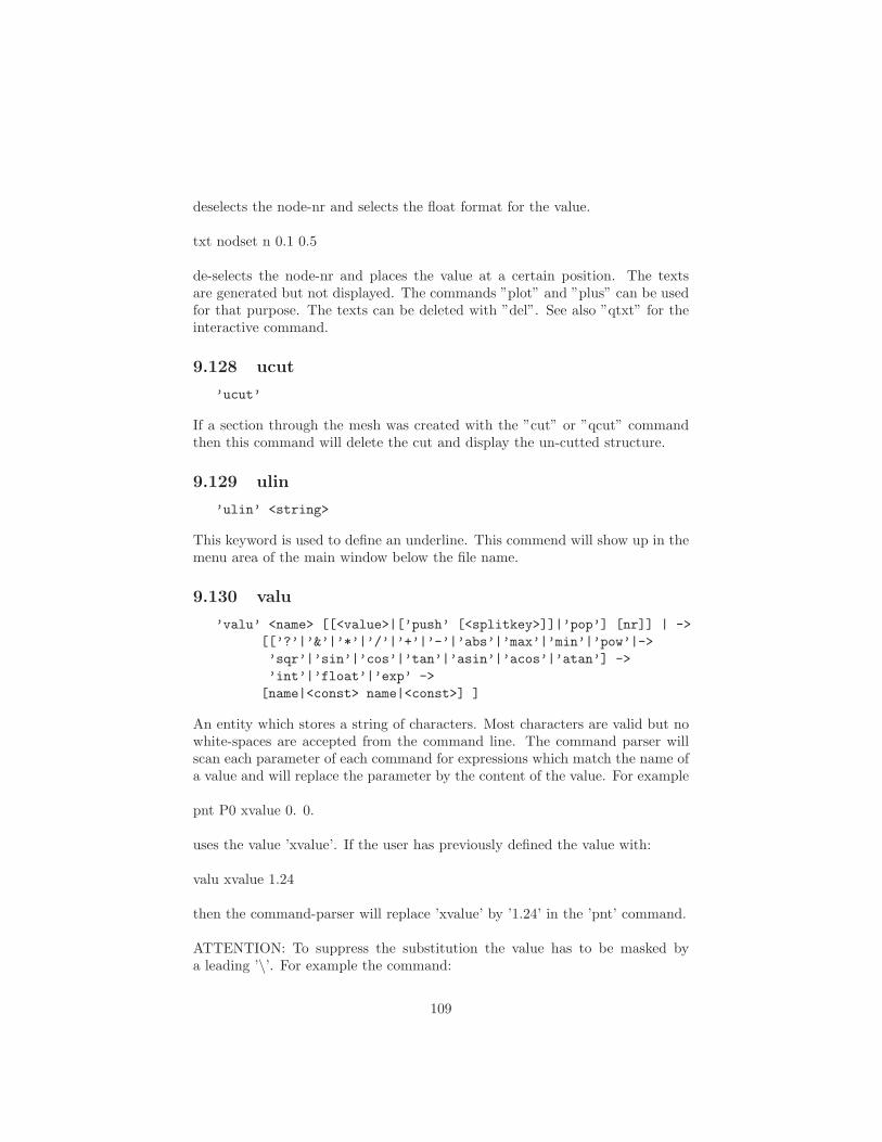
deselects the node-nr and selects the float format for the value.
txt nodset n 0.1 0.5
de-selects the node-nr and places the value at a certain position. The textsare generated but not displayed. The commands ”plot” and ”plus” can be usedfor that purpose. The texts can be deleted with ”del”. See also ”qtxt” for theinteractive command.
9.128 ucut
’ucut’
If a section through the mesh was created with the ”cut” or ”qcut” commandthen this command will delete the cut and display the un-cutted structure.
9.129 ulin
’ulin’ <string>
This keyword is used to define an underline. This commend will show up in themenu area of the main window below the file name.
9.130 valu
’valu’ <name> [[<value>|[’push’ [<splitkey>]]|’pop’] [nr]] | ->
[[’?’|’&’|’*’|’/’|’+’|’-’|’abs’|’max’|’min’|’pow’|->
’sqr’|’sin’|’cos’|’tan’|’asin’|’acos’|’atan’] ->
’int’|’float’|’exp’ ->
[name|<const> name|<const>] ]
An entity which stores a string of characters. Most characters are valid but nowhite-spaces are accepted from the command line. The command parser willscan each parameter of each command for expressions which match the name ofa value and will replace the parameter by the content of the value. For example
pnt P0 xvalue 0. 0.
uses the value ’xvalue’. If the user has previously defined the value with:
valu xvalue 1.24
then the command-parser will replace ’xvalue’ by ’1.24’ in the ’pnt’ command.
ATTENTION: To suppress the substitution the value has to be masked bya leading ’\’. For example the command:
109

del v \value
will delete the value itself. The content of a value can be defined by the user
valu arg1 1.24
or derived from the stack previously filled by a command
valu arg1 pop
if the ”stack” was activated. A certain number on the stack can be addressedwith
valu arg1 pop 2
were the ’2’ means that 2 successive ’pops’ are executed. In this way the secondvalue on the stack can be loaded at once.
Values can be added to a set
seta valset v all
and can then be deleted by zapping “zap” the set storing the values.Values can be written to the stack when the ’push’ parameter is used:
valu arg1 push
A white-space separated string stored in a “valu” will be written to the stack inseparate sub-strings. With this method single pieces of a white-space separatedstring can be splitted and stored in separate values:
stack on
opens the stack
valu complicatedString push
splits the string stored in ’complicatedString’ and writes the single pieces tothe stack. The command
valu subString pop 3
loads the 3rd substring into the varible ’subString’. Other splitting charac-ters can be used when this character follows the push key-word:
valu string push .
110

splits the string at each occurence of “.” and writes the pieces to the stack.The command is able to perform simple calculations like
valu result * arg1 arg2
’result’ will store the product from ’arg1’ and ’arg2’. The two arguments arg1and arg2 may be other ’values’ or constant numbers. That means that a directmultiplication of two numbers or a value with a number is possible. During thecalulation the strings are converted to double precision numbers and the resultis stored as a string representing an exponential number. The ’int’, ’float’ and’exp’ convert between integer, floating point and exponential format:
valu result int result
The ’?’ operator is used to request user input:
valu string ?
The command is waiting for user input. Please type into the terminal. Usuallythis requires to leave the graphics window and click into the terminal from whichcgx was started.
The ’&’ operator is used to concatenate two strings:
valu string3 & string1 string2
The string1 and string2 might be values or constant strings.See also “prnt” and ”How to write values to a file”.
9.131 view
’view’ ’fill’|’line’|’point’ <value>|
’edge’ [’off’]|’elem’ [’off’]|’surf’|’volu’|
’front’|’back’|’vec’ [’off’]|’disp’ [’off’]|
’bg’ [’w’|’k’]|’sh’ [’off’]|’ill’ [’off’]
Commands to control the graphic output. This command is intended for batch-mode. See also ”Viewing” for the menu controlled functions.
• ”fill” Element-faces are filled
• ”line” Elements are displayed as fireframes
• ”point” Element-edges are displayed as points with a pixel-width of ’value’
• ”edge” triggers the display of the model edges were
111

• ”elem” triggers the display of the element edges. They are deselected withthe additional parameter ”off”.
• ”surf” and ”volu” are used to display the structure either only by it’souter skin (surf) or by drawing all elements (volu).
• ”front” and ”back” define which side of the structure should be drawn.Either the side which faces the user or the back-side. If the back-side isdisplayed then internal structures are visible.
• ”vec” triggers the vector mode. All vector-entities like displacements aredisplayed with arrows pointing in the direction of the vector and with alength proportional to the value of the vector. See ”Toggle Vector-Plot”for a detailed description of the equivalent menu-function.
• ”disp” will show the deformed structure based on a formerly selected dis-placement dataset (no entity must be selected). See ”Toggle Add-Displacement”for a detailed description of the equivalent menu-function.
• ”bg” Without second parameter toggles the background colour. The sec-ond parameter ’w’ forces white while the parameter ’k’ forces black asbackground colour.
• ”sh” Shaded results are shown. Switched off with ”off”.
• ”ill” Illuminale the backface of the elements. Switched off with ”off”.
9.132 volu
’volu’ <set>
This keyword is used to calculate the volume and the center of gravity of a setof volume-elements. If an ccx-input file with density data was read then themass will be also calculated. If a ’dataset’ is active then an averaged value iscalculated.
The command writes to the ”stack”.
9.133 while
’while’ <value>|<const> ’eq’|’ne’|’==’|’!=’|’<’|’>’ <value>|<const>
A command to compare two values (’valu’ or constant numbers). If the compareis True the following commands are executed until the ’endwhile’ command isfound. This procedure is repeated until the compare is False.
while arg1 == arg2
will repeat the commands between ’while’ and ’endwhile’ until the numericalvalue stored in ’arg1’ is not equal to the numerical value stored in value ’arg2’.
112

The values are locally converted to ’float’ format for the numerical comparison.The ’eq’ and ’ne’ compare strings and should not be used for numerical valuessince no conversion to a common format is done. Two strings are equal if theyhave the same length and all characters are equal.
See also “if”, “valu”, “stack” and “How to run cgx in batch mode”.
9.134 wpos
’wpos’ <xp> <yp>
Positions the window on the screen were xp and yp are the coordinates in pixelrelative to the left upper corner. This command takes no effect during readingand execution of a batch file. It will be executed in the glut event loop (the glutlibrary [2] for window management and event handling).
9.135 wsize
’wsize’ [RETURN]|’f’]|[<xp> <yp>]
Size of the window were xp and yp are the size in pixel. Without argument thesize is the initial size and with the argument ’f’ (fullsize) the screen resolutionis used. This command takes ONLY effect during reading and execution of abatch file IF it is written in the very first line. Otherwhise it will be executedafter reading of the batch file in the glut event loop (the glut library [2] forwindow management and event handling) which means that the program hasto go into the interactive mode to take effect.
9.136 zap
’zap’ <set>
This keyword is used to delete all entities of a set and the set itself. All dependingentities will be deleted as well.
9.137 zoom
’zoom’ [<scale>]|[<p1x> <p1y> <p2x> <p2y>]
This keyword is used to scale the model in the window. For example
zoom 2
will increase the size of the representation of the model by a factor of 2. Acertain region of the model can be specified with two corner points of an imagi-nary rectangle. The coordinates are relative to the graphic-window which has itsorigin at the left/lower corner and as a fraction of the edge-lengths. For example
113

zoom 0. 0. 0.5 0.5
will display the third quadrant of the window scaled by a factor of 2.
114

10 Element Types
Node numbering of the elements and the type numbers used in the Result For-mat (frd-file). The solvers might use different node-numbering rules.
1
2
2 node beam element (be2, type 11)
115

1
2
3
3 node beam element (be3, type 12)
21
3
3 node shell element (tr3, tr3u, type 7)
116

21
3
4
56
6 node shell element (tr6, type 8)
21
34
4 node shell element (qu4, type 9)
117
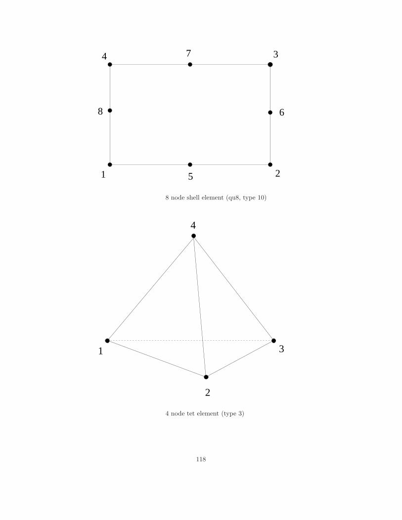
21
34
5
6
7
8
8 node shell element (qu8, type 10)
1
2
3
4
4 node tet element (type 3)
118
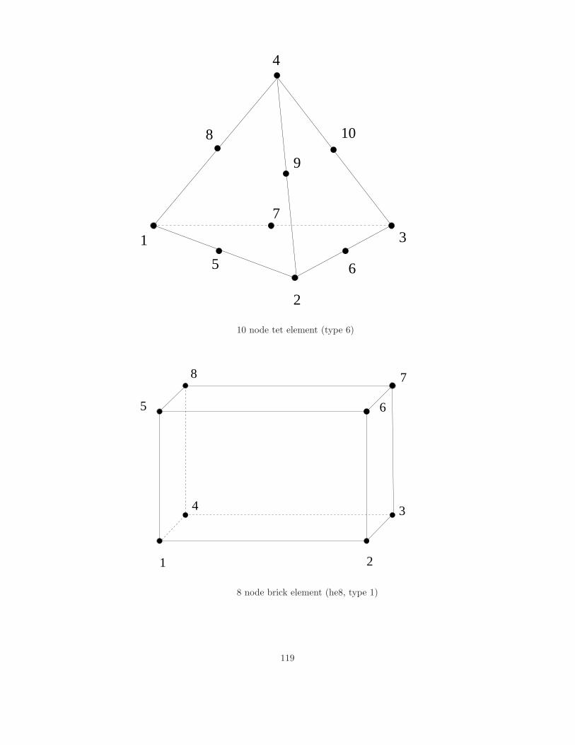
1
2
3
4
5 6
7
8 10
9
10 node tet element (type 6)
21
34
5 6
78
8 node brick element (he8, type 1)
119
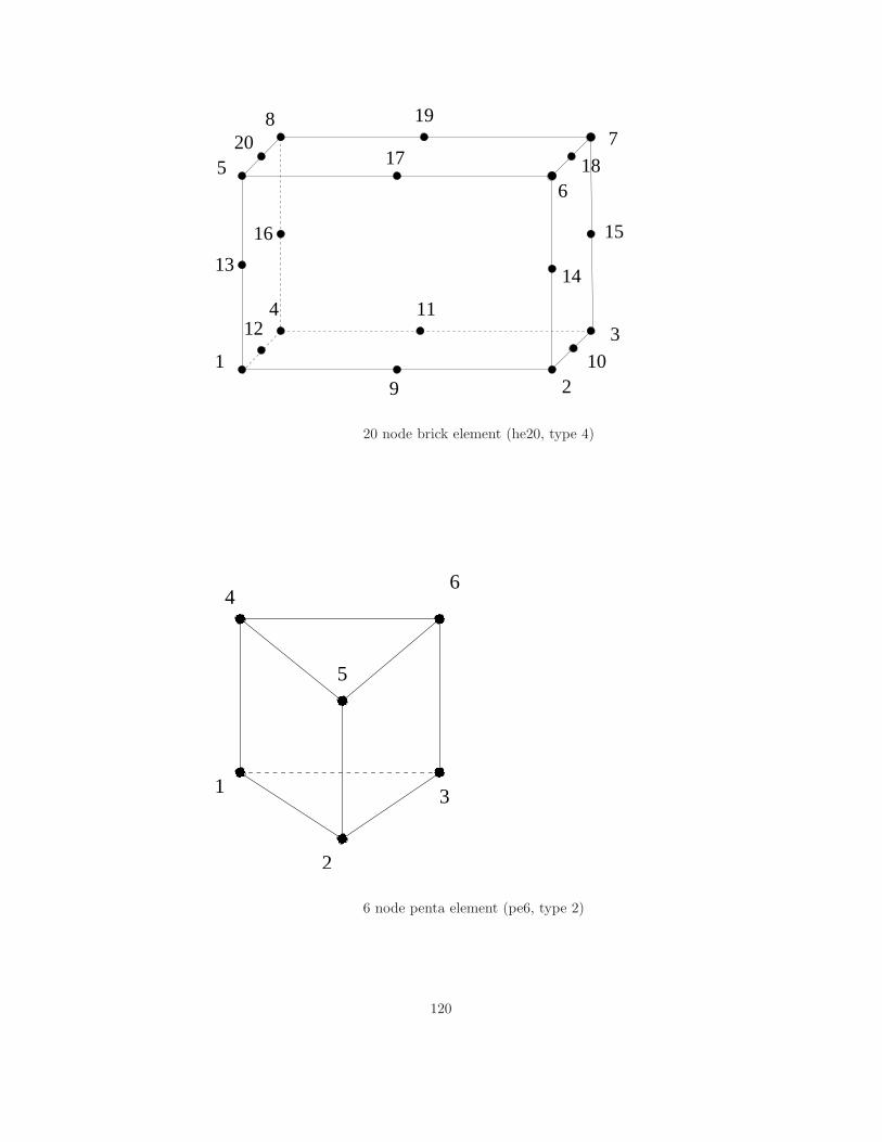
8
5
2
3
6
7
9
11
1314
1516
17 18
19
20
4
1
12
10
20 node brick element (he20, type 4)
1
6
5
4
3
2
��
����
��
����
����
6 node penta element (pe6, type 2)
120
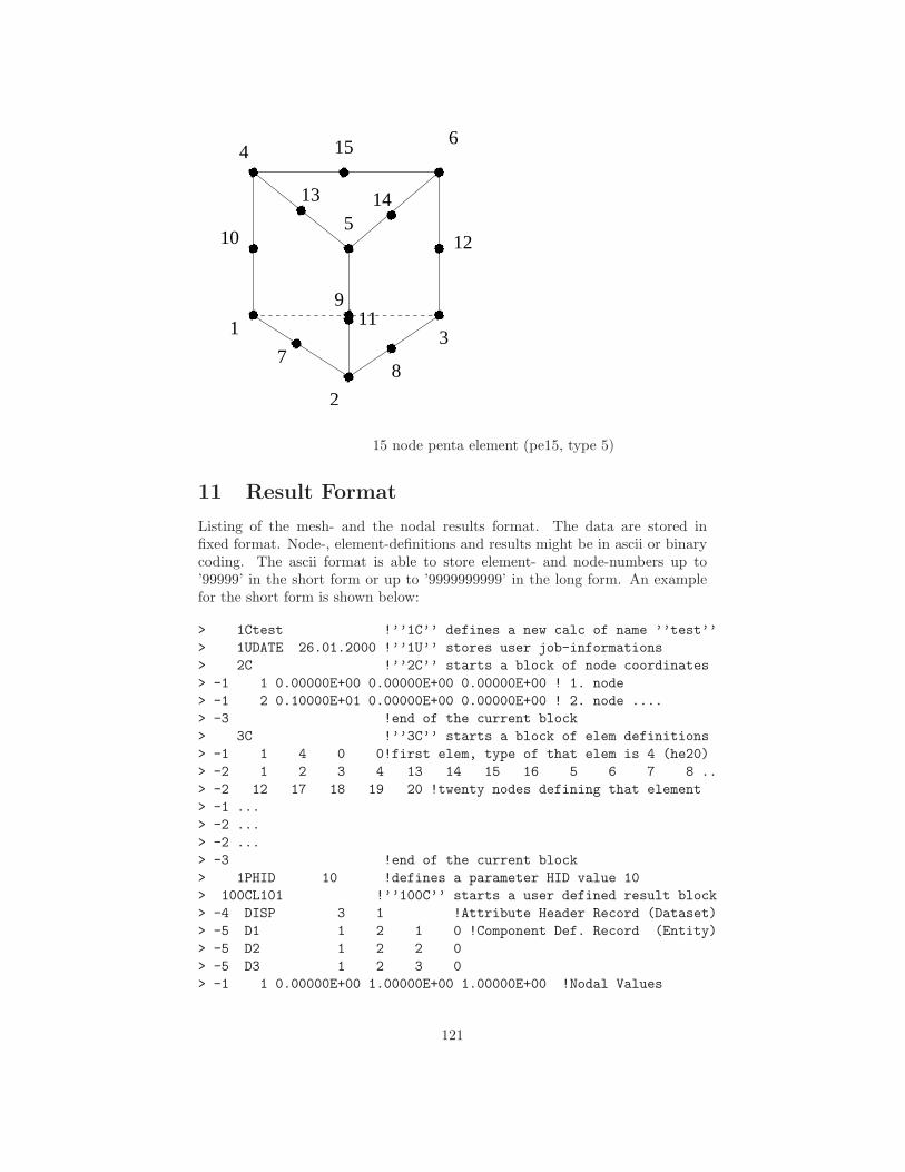
2
3
4
5
1
6
12
14
15
13
11
78
9
10����
����
��������
����
��������
��������
����
����
��
������
��������
����
��
����
15 node penta element (pe15, type 5)
11 Result Format
Listing of the mesh- and the nodal results format. The data are stored infixed format. Node-, element-definitions and results might be in ascii or binarycoding. The ascii format is able to store element- and node-numbers up to’99999’ in the short form or up to ’9999999999’ in the long form. An examplefor the short form is shown below:
> 1Ctest !’’1C’’ defines a new calc of name ’’test’’
> 1UDATE 26.01.2000 !’’1U’’ stores user job-informations
> 2C !’’2C’’ starts a block of node coordinates
> -1 1 0.00000E+00 0.00000E+00 0.00000E+00 ! 1. node
> -1 2 0.10000E+01 0.00000E+00 0.00000E+00 ! 2. node ....
> -3 !end of the current block
> 3C !’’3C’’ starts a block of elem definitions
> -1 1 4 0 0!first elem, type of that elem is 4 (he20)
> -2 1 2 3 4 13 14 15 16 5 6 7 8 ..
> -2 12 17 18 19 20 !twenty nodes defining that element
> -1 ...
> -2 ...
> -2 ...
> -3 !end of the current block
> 1PHID 10 !defines a parameter HID value 10
> 100CL101 !’’100C’’ starts a user defined result block
> -4 DISP 3 1 !Attribute Header Record (Dataset)
> -5 D1 1 2 1 0 !Component Def. Record (Entity)
> -5 D2 1 2 2 0
> -5 D3 1 2 3 0
> -1 1 0.00000E+00 1.00000E+00 1.00000E+00 !Nodal Values
121

> -1 2 1.00000E+00 0.00000E+00 0.00000E+00
> -3 !end of the current block
> 9999 !end of data
The binary format applys only for data lines and the “end of the current block”line (-3), which is omitted. All other lines are the same.
11.1 Model Header Record
Purpose: Defines the name of the model
Format:(1X,’ 1’,’C’,A6)
Values: KEY, CODE, NAME
11.2 User Header Record
Purpose: Stores additional user informations regarding the job
ie. user id, creation date, model informations
Format:(1X,’ 1’,’U’,A66)
Values: KEY, CODE, STRING
11.3 Nodal Point Coordinate Block
Purpose: Defines the nodal coordinates
1. Record:
Format:(1X,’ 2’,’C’,18X,I12,37X,I1)
Values: KEY, CODE,NUMNOD, FORMAT
Where: KEY = 2
CODE = C
NUMNOD = Number of nodes in this block
FORMAT = Format indicator
0 short format
1 long format
2 binary format, coordinates float
3 binary format, coordinates double
Following records (ascci, FORMAT=0 | 1):
Short Format:(1X,’-1’,I5,3E12.5)
Long Format:(1X,’-1’,I10,3E12.5)
Values: KEY, NODE, X,Y,Z
Where: KEY = -1
NODE = node number
X.. = coordinates
122
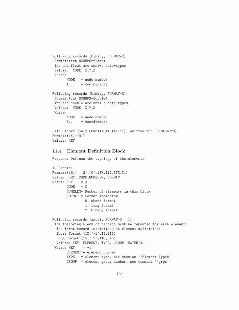
Following records (binary, FORMAT=2):
Format:(int NCOMPS*float)
int and float are ansi-c data-types
Values: NODE, X,Y,Z
Where:
NODE = node number
X.. = coordinates
Following records (binary, FORMAT=3):
Format:(int NCOMPS*double)
int and double are ansi-c data-types
Values: NODE, X,Y,Z
Where:
NODE = node number
X.. = coordinates
Last Record (only FORMAT=0&1 (ascii), omitted for FORMAT=2&3):
Format:(1X,’-3’)
Values: KEY
11.4 Element Definition Block
Purpose: Defines the topology of the elements
1. Record:
Format:(1X,’ 3’,’C’,18X,I12,37X,I1)
Values: KEY, CODE,NUMELEM, FORMAT
Where: KEY = 3
CODE = C
NUMELEM= Number of elements in this block
FORMAT = Format indicator
0 short format
1 long format
2 binary format
Following records (ascci, FORMAT=0 | 1):
The following block of records must be repeated for each element:
The first record initializes an element definition:
Short Format:(1X,’-1’,I5,3I5)
Long Format:(1X,’-1’,I10,3I5)
Values: KEY, ELEMENT, TYPE, GROUP, MATERIAL
Where: KEY = -1
ELEMENT = element number
TYPE = element type, see section ’’Element Types’’
GROUP = element group number, see command ’’grps’’
123

MATERIAL= element material number, see command ’’mats’’.
Then the nodes in the correct order have to follow:
Short Format:(1X,’-2’,15I5)
Long Format:(1X,’-2’,10I10)
Values: KEY,NODE,NODE,NODE,NODE, ...
Where: KEY = -2
NODE = node number
Additional lines must follow if more nodes are used.
Following records (binary, FORMAT=2):
Format:(4*int nodes*int)
int and float are ansi-c data-types
Values: ELEMENT, TYPE, GROUP, MATERIAL,NODE,NODE,NODE,NODE, ...
Where:
ELEMENT= element number
TYPE = element type, see section ’’Element Types’’
GROUP = element group number, see command ’’grps’’
MATERIAL= element material number, see command ’’mats’’.
NODE = node number
Last Record (only FORMAT=0 | 1 (ascii), omitted for FORMAT=2):
Format:(1X,’-3’)
Values: KEY
11.5 Parameter Header Record
Purpose: Stores informations related to datasets.
ie. bondary conditions and loads
They should consist of a keyword and a value
Format:(1X,’ 1’,’P’,A66)
Values: KEY, CODE, STRING
Where: KEY = 1
CODE = P
STRING = Keyword Value (ie: FORCE 1000.)
11.6 Nodal Results Block
Purpose: Stores values on node positions
1. Record:
Format:(1X,’ 100’,’C’,6A1,E12.5,I12,20A1,I2,I5,10A1,I2)
124
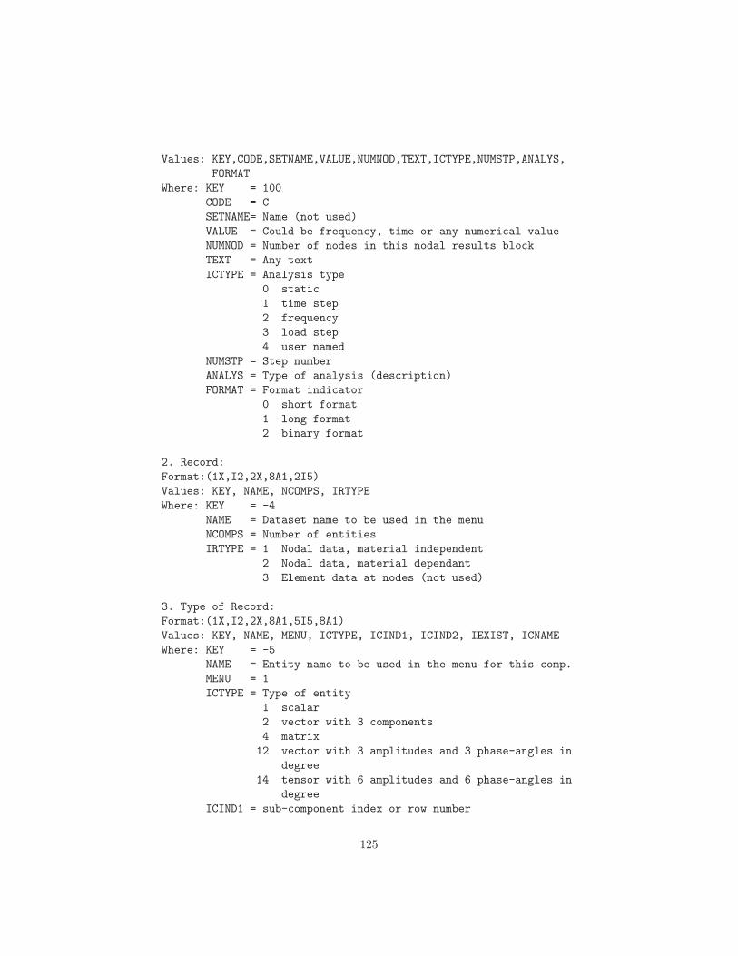
Values: KEY,CODE,SETNAME,VALUE,NUMNOD,TEXT,ICTYPE,NUMSTP,ANALYS,
FORMAT
Where: KEY = 100
CODE = C
SETNAME= Name (not used)
VALUE = Could be frequency, time or any numerical value
NUMNOD = Number of nodes in this nodal results block
TEXT = Any text
ICTYPE = Analysis type
0 static
1 time step
2 frequency
3 load step
4 user named
NUMSTP = Step number
ANALYS = Type of analysis (description)
FORMAT = Format indicator
0 short format
1 long format
2 binary format
2. Record:
Format:(1X,I2,2X,8A1,2I5)
Values: KEY, NAME, NCOMPS, IRTYPE
Where: KEY = -4
NAME = Dataset name to be used in the menu
NCOMPS = Number of entities
IRTYPE = 1 Nodal data, material independent
2 Nodal data, material dependant
3 Element data at nodes (not used)
3. Type of Record:
Format:(1X,I2,2X,8A1,5I5,8A1)
Values: KEY, NAME, MENU, ICTYPE, ICIND1, ICIND2, IEXIST, ICNAME
Where: KEY = -5
NAME = Entity name to be used in the menu for this comp.
MENU = 1
ICTYPE = Type of entity
1 scalar
2 vector with 3 components
4 matrix
12 vector with 3 amplitudes and 3 phase-angles in
degree
14 tensor with 6 amplitudes and 6 phase-angles in
degree
ICIND1 = sub-component index or row number
125

ICIND2 = column number for ICTYPE=4
IEXIST = 0 data are provided
1 data are to be calculated by predefined
functions (not used)
2 as 0 but flaged by cgx
ICNAME = Name of the predefined calculation (not used)
ALL calculate the total displacement if ICTYPE=2
This record must be repeated for each entity.
4. Type of Record: (not used)
This record will be necessary in combination with the request for
predefined calculations. This type of record is not allowed in
combination with binary coding of data.
Format:(1X,I2,2I5,20I3)
Values: KEY,IRECTY,NUMCPS,(LSTCPS(I),I=1,NUMCPS)
Where: KEY = -6
IRECTY = Record variant identification number
NUMCPS = Number of components
LSTCPS = For each variant component, the position of the
corresponding component in attribute definition
5. Type of Record:
The following records are data-records and the format is repeated
for each node.
In case of material independent data
- ascii coding:
Following records (ascci, FORMAT=0 | 1):
Short Format:(1X,I2,I5,6E12.5)
Long Format:(1X,I2,I10,6E12.5)
Values: KEY, NODE, XX..
Where: KEY = -1 if its the first line of data for a given node
-2 if its a continuation line
NODE = node number or blank if KEY=-2
XX.. = data
- binary coding:
Following records (ascci, FORMAT=2):
(int,NCOMPS*float)
int and float are ansi-c data-types
Values: NODE, XX..
Where:
NODE = node number or blank if KEY=-2
XX.. = data
126

In case of material dependant data
REMARK: Implemented only for NMATS=1
- first line:
Short Format:(1X,I2,4I5)
Long Format:(1X,I2,I10,3I5)
Values: KEY, NODENR, NMATS
Where: KEY = -1
NODENR = Node number
NMATS = Number of different materials at this node(unused)
- second and following lines:
Short Format:(1X,I2,I5,6E12.5)
Long Format:(1X,I2,I10,6E12.5)
Values: KEY, MAT, XX, YY, ZZ, XY, YZ, ZX ..
Where: KEY = -2
MAT = material-property-number if KEY=-2 (unused)
XX.. = data
Last Record (only FORMAT=0 | 1 (ascii), omitted for FORMAT=2):
Format:(1X,’-3’)
Values: KEY
12 Pre-defined Calculations
Listing of the automatically calculated additional results.
12.1 Von Mises Equivalent Stress
Entity name: Mises
σvM =1√2
√
(σx − σy)2 + (σy − σz)2 + (σz − σx)2 + 6τ2yz + 6τ2zx + 6τ2xy
12.2 Von Mises Equivalent Strain
Entity name: Mises
ǫvM = 2/3 ∗ 1√2
√
(ǫx − ǫy)2 + (ǫy − ǫz)2 + (ǫz − ǫx)2 + 6ǫ2yz + 6ǫ2zx + 6ǫ2xy
12.3 Principal Stresses
Entity names: PS1, PS2, PS3, worstPS
127
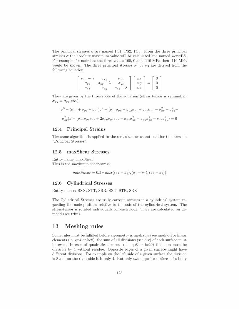
The principal stresses σ are named PS1, PS2, PS3. From the three principalstresses σ the absolute maximum value will be calculated and named worstPS.For example if a node has the three values 100, 0 and -110 MPa then -110 MPawould be shown. The three principal stresses σ1 σ2 σ3 are derived from thefollowing equation:
σxx − λ σxy σxz
σyx σyy − λ σyz
σzx σzy σzz − λ
nxnynz
=
000
They are given by the three roots of the equation (stress tensor is symmetric:σxy = σyx etc.):
σ3 − (σxx + σyy + σzz)σ2 + (σxxσyy + σyyσzz + σzzσxx − σ2
xy − σ2
yz−
σ2
zx)σ − (σxxσyyσzz + 2σxyσyzσzx − σxxσ2
yz − σyyσ2
zx − σzzσ2
xy) = 0
12.4 Principal Strains
The same algorithm is applied to the strain tensor as outlined for the stress in”Principal Stresses”.
12.5 maxShear Stresses
Entity name: maxShearThis is the maximum shear-stress:
maxShear = 0.5 ∗max((σ1 − σ3), (σ1 − σ2), (σ2 − σ3))
12.6 Cylindrical Stresses
Entity names: SXX, STT, SRR, SXT, STR, SRX
The Cylindrical Stresses are truly cartesin stresses in a cylindrical system re-garding the node-position relative to the axis of the cylindrical system. Thestress-tensor is rotated individually for each node. They are calculated on de-mand (see trfm).
13 Meshing rules
Some rules must be fulfilled before a geometry is meshable (see mesh). For linearelements (ie. qu4 or he8), the sum of all divisions (see div) of each surface mustbe even. In case of quadratic elements (ie. qu8 or he20) this sum must bedivisible by 4 without residue. Opposite edges of a given surface might havedifferent divisions. For example on the left side of a given surface the divisionis 8 and on the right side it is only 4. But only two opposite surfaces of a body
128

can use this feature. These surfaces are called top and bottom surfaces. Allother surfaces of this body must have unique divisions on opposite edges. Incase of 3 sided surfaces it is necessary to apply a minimum division sufficientfor two elements along the edge. The only exception is the element tr3u (seeelty) which allows a division of one.
A body can not be meshed when the shape of the body is very far from beingbrick-like. The body might be subdivided to improve the shapes of the singleones. There is a restriction for the definition of five- or seven-sided bodies. Thefirst two surfaces in the body-topology (see gbod) have to be defined in thesame order. That means the first line of the first surface has to be connectedwith the first line in the second surface by one of the remaining surfaces. Thisis always the case if the body is a product of a ”swep” command.
14 User-Functions
The user might define his own functions to manipulate the mesh or the re-sults with the user function stored in file ”userFunction.c”. See the command”call” how to call a user function. The user can generate new nodes, elementsor datasets or extend or manipulate existing datasets or interfaces to othersoftware. The file ”userFunction.c” includes an example which calculates thehydrostatic stress and stores the result in a new dataset. There the user can seehow to deal with datasets.
A Known Problems
A.1 Program is not responding
If the program seems to hang then leave the window with the mouse pointerand go in again. If that does not help then probably a command is waiting forinput. Stay with the mouse pointer inside the window and press the ”q” keyseveral times. Another very popular error is to move the mouse-pointer intothe xterm were the typed commands and the protocol is visible. Please, themouse-pointer MUST stay in the main-window during typing!
A.2 Program generates a segmentation fault
Write a mail to the author and, if possible, add the input-file.[3].
B Tips and Hints
The following collection will give you background information and proceduresto deal with common situations.
129
B.1 How to change the format of the movie file
Use a shell command like convert to split up movie.gif with multiple layers intomultiple frames, as seperate jpeg files:
convert movie.gif %d.jpg
Convert any series of multiple jpeg files into WMV format with:
mencoder ’mf://*.jpg’ -mf type=jpg:fps=25 -ovc lavc -lavcopts
vcodec=wmv2 -o movie.wmv
To convert a video file into avi format use this command:
mencoder <videofile> -ovc lavc -lavcopts vcodec=flv -of avi -o movie.avi
In general:To convert a video file from one format into the other, use the program”mencoder”. It comes with the mplayer packages.
mplayer movie.wmv
B.2 How to get the sets from a geo- or ccx-inp file forpost-processing
Quite often it is usefull to have the already defined sets from the pre-processingor/and the calculation available when doing the post-processing of results. Thesets defined in the ccx-input file (.inp) can either be read together with theresults (.frd) at start-up:
cgx results.frd input.inp
or the user may read them during run-time
read input.inp nom
(see “read”). When it comes to the sets defined in the geo file a slightly differentapproach is needed. The geo file must be read before the result file. So the userstarts cgx in the build mode
cgx -b geofile.fbd
meshes the model (see “mesh”) and then read the results
read results.frd nom
and optionally the input file. Be aware that the parameter “nom” is essen-tial here. Use “prnt” to get an overview over the available sets.
130
B.3 How to define a set of entities
Some knowledge is necessary to efficiently select entities (nodes, points ..). As agolden rule in complicated situations never try to create a set just by ”adding”the entities to the set (see qadd). It is much better to catch a bigger groupwhich includes certainly the wanted ones. Then display the set with the plotcommand and remove all unwanted entities with the qrem command. Entitiesare selected if at least one pixel of it is inside the selection rectangle. But thereis one exception: Only the lower left corner of any text (names of points etc.)can be selected. Surfaces can also be selected by picking its shaded interiour(see “rep)”. You might add all lower entities (as points for example) by typing”comp set do”. This is necessary for example if you had selected surfaces andyou want to move them in space. Only points have locations and thereforenothing will happen unless you completed the set by the related points with”comp” command.
There is another type of set called sequence. The data-structure is the samebut with one exception, the data keep their order in which they were selected.This type of set is used for splines (see ”qlin” and ”line”) or in combinationwith the ”graph” command if values along a path should be displayed. Use”prnt sq” to list all existing sequences and use ”qseq” or ”seqa” to create them.Up to now they are only used to store nodes and points. As sets they will bewritten to a file if fbd format is specified. In this case also node-sequences canbe stored.
B.4 How to enquire node numbers and values at certainlocations
A very common problem is how to get the exact value on a node position duringpost-processing. To actually get the value add the element edges to the view(see Toggle Element Edges) and type qenq and press the RETURN key (duringtyping the mouse-pointer MUST stay in the main window, do NOT move thepointer into the xterm). Then move the mouse-pointer over the location of anode and press the ”n” key. The node-number, the value at that node and thelocation will be written in the xterm from which the cgx was started. See alsothe ”enq” command for batch controlled value extraction.
B.5 How to write values to a file
When you need to write certain values (see “valu”) to a file you may use the’echo’ system command:
• Choose the relevant dataset (menu or ds command)
• Add the relevant nodes to a set (qadd setname or seta setname n ..)
• Open the stack: stack on
• Place node-values on the stack: prnt se setname
131
• Store the node: valu nod1 pop
• Store the value: valu val1 pop
• Write to file: sys echo Node nod1 Value val1 >| file.txt
See also “if” and “while” and see the demo in “If and while demo” on how towork with this commands. They are usefull for automatic post-processing.
B.6 How to select only nodes on the surface
Some times you need to select nodes only on the surface of the mesh. This can bedone when the mesh is displayed in the surface mode (see ”Toggle Surfaces/Volumes”)using the menu-entry ”Show Elements With Light”. To find node positionsmore easily add the element edges to the view (see Toggle Element Edges).
A different way uses the element-faces (see ”plot” with parameter ”f”). Storethe desired faces in a new set (qadd) and complete the set downwards (“compset do”). Check the selected nodes with “plot n setname”.
B.7 How to generate a time-history plot
So called time history plots can be created based on a previous displayed se-quence of data-sets (see ”Toggle Dataset Sequence”) with the command ”graph”.It is also possible to use only the command line. For example:
• ds 1 e 3
• ds 1 2 10
• graph set t
will produce a time history plot for the nodes stored in set over all loadcasesfrom 1 to 10 for the entity nr 3. Or
• graph set t DISP D1
will display the displacement in direction 1 for all loadcases. For more detailsand other options look into the ”graph” command description.
132
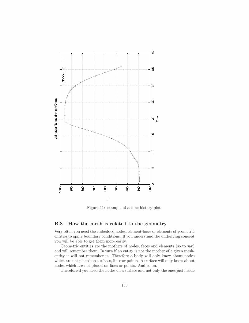
Figure 11: example of a time-history plot
B.8 How the mesh is related to the geometry
Very often you need the embedded nodes, element-faces or elements of geometricentities to apply boundary conditions. If you understand the underlying conceptyou will be able to get them more easily.
Geometric entities are the mothers of nodes, faces and elements (so to say)and will remember them. In turn if an entity is not the mother of a given mesh-entity it will not remember it. Therefore a body will only know about nodeswhich are not placed on surfaces, lines or points. A surface will only know aboutnodes which are not placed on lines or points. And so on.
Therefore if you need the nodes on a surface and not only the ones just inside
133
the surface, then create a set with this surface and do a ”comp set do”. Thiswill add the lines and points together with their nodes to the set.
On the other hand if you have only a node and you need the geometric entityin which the node is embedded you might also type ”comp set do”.
B.9 How to change the order of elements
Use the command ”mids” to change from second order to first order or vice versa.In this case the amount of elements will not change. Or use the command ”send”with the parameter “quadlin” to change from second order to first order. Butin this case each second order element will be splitted in 8 first order elements.
B.10 How to connect independent meshes
Sometimes it is advisable to ”glue” independent meshes together instead oftrying to create one big seamless-mesh. Or you just want to create a contactformulation were you know that no separation will happen. In this situations youmight use equations (also called mpc’s) which connect one dependent node withone or more independent nodes. The independent side should be coarser thanthe dependent side to avoid gaps in the connection. See the command ”send incombination with the option ”areampc” how to create such connections. Slidingand fixed contact as well as press-fits can be modelled. The necessary sets shouldbe defined based on geometry not on the mesh. In this case the definition willbe stored with the ”save” or ”exit” command and can be used after the nextprogram call.
Background: The movement of each location in an element (or on its surface)is fully described by the movement of its associated nodes and its shape-function.In an iterative algorithm element-coordinates are varied until the real-worldcoordinates of a dependent node are matched. Based on the element coordinatesthe shape function gives the participation (weight) factors of the independentnodes (the coefficients in the mpc’s). This approach delivers valid results aslong as the dependent node is not located outside of the independent element.Therefore the location of the dependent node has to be modified in such cases.The dependent will be moved to the surface of the independent element (againdecribed by its shape-function) and the procedure is repeated.
B.11 How to define loads and constraints
Loads and constraints are not saved in any database. They are just createdand written to a file with the ”send” command. But the sets which are neededfor the definition are stored together with the geometry if you type the ”save”command. Of course the sets must have been defined based on geometry andnot based on mesh entities like nodes because mesh-entities are not saved withthe ”save” command. You must know that geometry-sets know also their meshentities after a ”mesh” command. If you store your commands to write theboundary conditions in a file you can easily repeat them by just reading this
134

Figure 12: Dependent node on element face to create a connection
command-file (see ”read”). Several types of loads can be applied. That isforces, pressure, thermal-heat-coefficients and radiation etc. For unsupportedloads write a set of element-, node- or face-labels (parameter ”names”) and applythe desired load to that set in the solver input-file. Other boundary conditionslike single-point-constraints for structural, thermal and fluid-calculations can bewritten. The sliding condition (parameter ”slide”) were nodes are bound to theelement-faces to which they belong can be used for structural calculations orfor fluid calculations. In the later case it forces the flow to follow the surfaceof the elements. This is necessary in inviscid calculations to prevent the fluidto penetrate the walls. Results from a previous calculation can be written inthe solver input format for further calculations (parameter ”ds”, ”tmf” etc.).For example temperatures for thermal mechanic fatigue analysis or velocities,pressures and thermals for a restart of a cfd calculation.
B.12 How to map loads
Values at nodes can be mapped (interpolated) from a second mesh with the”map” command. This second mesh (data source or “master”) is usually avail-able as a result-file from a previous calculation. The ”read” command with the“add” parameter can be used to include this file in the current model. Solver-input files (inp) and result files (frd) can be used as a data source. The command
135
will add an offset to the nodes and elements so that existing nodes and elementswill not be overwritten. The original mesh is the target or “slave” of the map-ping process. The mapping process will add the values to the dataset(s). Themapped values can be visualized by selecting the mapped dataset and entity andthen by plotting the slave elements or faces with “plot fv slave”. An exampleof the necessary commands for the mapping process (2D to 2D) is listed below:
Define a set with the slave nodes or faces. For example with:
qadd slave
comp slave do (to extend the set by the referenced faces or
nodes)
Then open a set and read the master-model:
seto new
read result.frd add
setc
If necessary move ’new’ in space to match the position of the
slave (see ‘‘move’’).
Add the faces to the ’new’ set
(only nodes and elements are already stored in "new"):
comp new do
plot f new
Define the master set:
qadd master (catch the right faces)
comp master do
Map the values of dataset 1 with:
map slave master surf ds1
Check the mapping with:
ds 1 e 1
plot fv slave
Write the file with the mapped values:
send slave abq pres ds1 e1
Check the file ‘‘slave_ds1e1.dlo’’ with an editor and use it
in an inp-file.
If the master values are not available in either inp or frd format but in anyother format which can be read by cgx (isaac, openFoam ..) it is then possibleto write them in frd format with the ”send” command.
136

B.13 How to run cgx in batch mode
Most commands can be executed in batch-mode. Actually if you read a file withgeometry (fbd-file) then you run cgx in batch mode already! You just have toadd ”exit” or ”quit” at the end of the file and it will be obvious. You might usethe ”read” command in such a command-file to reference other command-filesor to read files with mesh-entities for whatever purposes. In such a way youcan create and modify geometry or meshes in batch-mode or evaluate resultsin batch-mode. But you need a graphic-capable computer because cgx needs italso if no graphic output is requested. Nevertheless the pop up of the graphicwindow can be suppressed by starting cgx with the “-bg” parameter.
Some commands make only sense in a batch file like “if” and “while”. Pleasehave a look into “If and while demo” on how to work with this commands.Results can be extracted and stored to a file, see “How to write values to a file”.
Be aware of the ’examples’ directory. It holds examples on how to use thecommand language as a programming language. The ’ifwhiledemo’ generatespoints in a loop and shows how to write cgx generated values to a file. The’userDataset’ shows how to generate a user dataset for a temperature field basedon the z coordinate of the nodes.
It should be noted that a successive ’save’ or ’exit’ command will overwritethe batch file if it has the file-extension ’fbd’. To prevent this the user shoulduse a different extension like ’fbl’.
When executing commands which increase the used space then it might hap-pen that geometry is clipped and can not be seen or accessed anymore. In sucha case a “frame” command is needed. This command is usually automaticallytriggered. Especially in batch mode without graphic output it solves sometimesstrange situations.
If the command “init” or “wsize” is used then they have to be used in thevery first line. Otherwhise the window dimensions take only effect after thebatch file was completely parsed and executed.
B.14 How to process results
The node results can be modified or used to generate derived results. There arebasically three levels of operations.
The easiest one is to just multiply with a factor, add a number or use anexponent to all node results of a certain dataset with the ”ds” command.
The next level is using variables which can be used to do calculations basedon results and can be written back to an existion dataset or a new one. Thisrequires a good knowledge of the way cgx works and of the necessary commands(”if”, ”while”, ”stack”, ”valu”, ”enq”, ”prnt”, ”ds”, ”sys” etc.). In this way datacan be written to a file with the “sys” command (using echo) were an externalprogram might be invoked by the “sys” command which in turn could providedata for cgx.
Finally, complex operations can be coded in C in the file userFunction.c.The user function is activated by the ”call” command. A new compilation of
137

cgx is required unless a dynamically linked library is used.
B.15 How to deal with cad-geometry
In general hexahedra-elements perform better than tets but if the mesh shouldbe derived from a cad-geometry it is often more convenient to create a tetrahedramesh as to modify or rebuild the geometry to make it meshable with hexahedra-elements. The following section gives some hints which alternatives are available.
• The CAD format is supported by a stand alone translator (see the calculixhome pages). In this case the user can mesh the surfaces with structured-[13] (elty setname tr3 etc.) or unstructured triangles [14] (elty setnametr3u etc.). The user might modify this surface mesh until he is happy withit. The surface mesh can then be filled with tets created by an externalauto-mesher called from within cgx (mesh setname tet). The cgx uses thetet-mesher from NETGEN [4] for this task.
Therefore cgx can only generate a tet-mesh if NETGEN is installed and theprogram ng vol (part of NETGEN) is accessible. For the full functionallityreplace the original ng vol in the NETGEN package with the modifiedprogram ng vol from the cgx-distribution and build it again. This versionregards a target element size.
• For CAD models in STEP- or IGES-format you may consider to use atet-mesher like NETGEN [4] which often generates quite nice tet-mesheswith very few user interaction. You can read this meshes with cgx andcombine them with cgx-geometry and meshes. Then create your boundaryconditions etc. You might read the native-netgen format (.vol) instead ofabaqus-format because this includes the 2D meshing regions in separatesets which can be used to apply boundary conditions (“cgx -ng file.vol”,see ”Program Parameters”). See “prnt” how to list the available sets.
• A simple step-reader is integrated in cgx (cgx -step filename). It can dealwith points and lines. This is sufficient for axis-symmetric structures likea rotor but the experienced user might also use the following approach formore complex geometries: You start with a file containing a 2D-section,subdivide it in mesh-able surfaces and sweep it in the 3rd dimension tocreate your geometry (see swep). If features exist in the 3rd dimensionthen this features must be included in the 2D-section. Sweep the 2D-section to the location were the feature starts, then right to the end andat last to the end of the geometry. Delete the unwanted bodies beforeand after the feature. You might project the sweped sections to a targetsurface if the feature is shaped in the 3rd dimension (see proj).
Sometimes the geometry consists of several (maybe even identical) partswhich are arranged on different positions in space. This is called assembly.When cgx is started with the parameter “-stepsplit” instead of “-step”it will write the single parts to separate directories using their original
138

coordinate systems. The user can prepare meshable geometry or meshesbased on them. But he must use the filenames which he finds there. Thefinal meshed assembly can be build afterwards by calling the fbl-file whichwas written by cgx. This fbl-file contains the original step-commands toposition and eventually duplicate the single geometries/meshes from thesubdirectories.
The following section describes the process to generate a tet-mesh with cgxbased on a cad model:
Figure 13: CAD-geometry meshed with tet-elements
• Install and use the propper interface program to convert the cad format tofbd format (You find example data (vda,iges,step) in CalculiX/cgx x.x/examples/cad)
(ie: vda2fbd halter.vda > halter.fbd).
Remark: In some cases the header of the vda file causes trouble and mustbe modified to make the program run.
• Start cgx with that file (cgx -a halter.fbd). Usually some warnings appearon the screen but the program will fix that automatically (triggered bythe parameter -a). After all geometry has been read the program willmerge points and lines to close the volume. If problems occur the usermight start the program with option -b instead of -a (cgx -b halter.fbd).Then no automatic post-processing is done and the user has to preparethe geometry manually. See the commands merg, div, qdiv, qlin, rep.
139

• Then all nurbs related surfaces might be shaded (optional, the openGLextension library GLu is used for that matter). This has to be donemanually by typing first “rep all” and then “plus si all”. The whole processmight need some time. If a surface points inwards it is not illuminatedand appears only dark grey. Flip the surfaces in a way that its normaldirection points outwards (use ”qflp”. Press the ”a” key to selet the “all”mode and then select a correctly oriented surface by pressing key ”s”, allother surfaces will immediatelly use the same orientation). The orientationfix can also be done later after the surface mesh is available by selectinga wrong oriented element (dark grey) with ’qflp’ (key “e”).
• Define the element type (see elty). In most cases it is advisable to usetriangles first (tr6u) and not directly tetraeders (te10) because this hasthe advantage that the surface mesh can be interactively improved beforethe tets are generated. Remark: If you choose tets from the beginning,you must identify a set which holds an existing body (if only one bodyexists, its the set ’all’) or you must create a body with “body ! all” beforeyou can assign tets using the “elty” command.
• Type the command ”mesh all” to generate the surface-mesh (see mesh).
• Visualize and check the mesh (”plot f all“). If the command ”prnt info”lists ”ed:0” then the mesh is closed and ready to be used for tet meshing.
• If some surfaces can not be meshed then modify the divisions of the linesof this surfaces (see ”qdiv” or ”qmsh”) or chose the structured elementtype tr6 for this surfaces. Or define a certain element-size transition with“elty”. See especially the command ”qmsh” to fix parts of the surface-mesh in a convenient way since this command combines several other ones(for convenient usage of “qmsh” display the elements “plot e all y“ togetherwith faces “plus f all“ and add the lines with “plus lp all r“ and “plus ldall r“). You may switch on the element edges with ”view” elem.
In some cases surfaces are not meshable when you combined surfaces with“qmsh”. The referenced NURBS might be too small to cover the wholesurface. Without such a related nurbs no unstructured mesh can be cre-ated. If structured elements are no solution you may delete the relatedNURBS from the surface definition with ”qsur” and key ’b’. Then storethe surface in a set and create a new NURBS with “nurs ! setname”.The surfaces stored in the set will produce NURBS based on the Coonsalgorithm [13]. If the surface shape matches a primitive shape you mayalso use the ”qshp” or ”shpe” command to assign the matching shape.
• Generate the tet mesh (“mesh all tet“). A target-size for the tet-elementscan be specified if “ng vol” from the cgx distribution was installed (forexample “mesh all tet 2.5“ will define a maximum element-size of “2.5”).If the model consists of several unconnected parts separate them in singlesets and mesh one after the other (see seta, qadd, qrem, comp).
140
• Create sets of nodes, faces or elements to create boundary conditions (ifyou had not created them already based on the geometry) and exportthem with ”send”.
• Create the input deck for ccx with an editor and start the calculation.
• Look at the results with cgx (cgx results.frd).
B.16 How to check an input file for ccx
A quick check of a ccx input-file can be done with cgx by reading the file withthe option -c (cgx -c file.inp). After startup all defined node-, element-, andsurface-sets are availabe together with internal sets which group togeter certainentities according to their purposes. The following internal sets will be createdif appropriate data were found:
• +bou(DOF): Created if *BOUNDARY is found. All affected nodes arestored in +bou were +bou(DOF) store just the nodes which are con-strained in the related DOF number.
• +dep(BOU): Created if *EQUATION is found. All dependent nodes arestored in +dep.
• +ind(BOU): Analog to +dep.
• +clo[nr]: Created if *CLOAD is found. The nr counts the number ofappearance.
• +dlo[nr]: Created if *DLOAD is found.
• +mpc[nr]: Created if *MPC is found.
• +rad[nr]: Created if *MPC is found.
• +flm[nr]: Created if *FILM is found.
• +cflx[nr]: Created if *CFLUX is found.
• +dflx[nr]: Created if *DFLUX is found.
• +tie[1—2]: Created if *TIE is found. The set +tie1 stores the slave entitiesand +tie2 the master. The single sets which define the contact areas arelinked together so if identified with the “qenq” command the referenced(linked) opposing set is listed in the xterm.
• +trans...: Created if *TRANSFORM is found. The name consists of thedefinition of the transformation.
• +[elty]: Created for all known element types like *C3D20.
141

Check the element quality with “Show Bad Elements” or use “eqal” to setthresholds and “plot” or “prnt” to actually plot or list the affected elements.
Forces regard their referenced coordinate-system (*TRANSFORM). The val-ues are automatically transformed into the global cartesian system so that thevectors point in the correct direction.
Multiple load definitions inside one *STEP on a single entity will sum up(ccx compatible). This applies to cflux, dflux, cload, dload.
B.17 Remarks Concerning Ansys
The cgx is capable to write the following mesh entities to files (see “send”, thenecessary key-parameters are listed in brackets below):
• Nodes and Elements
• Sets of nodes and elements (nam)
• Single point constraints (spc)
• Equations (areampc)
• Pressure (pres)
• Temperatures (ds, all datasets with just one entity will be written astemperatures)
The resulting files have to be combined with the help of an editor and extendedby material-data and the necessary controll-commands.
So far results can not be read.
B.18 Remarks Concerning Code Aster
From Paul CARRICO (2005/02/12)Brief presentation of CODE ASTER: Code Aster is an implicit solver under
GPL licence from the French company EDF (Electricite de France).Code Aster and its documentations is downloadable at the following address:
http://www.code-aster.org
(NOTA : the documentation is in French at the moment but many users aretranslating it in English and in German)
The following list is not exhaustive but it briefly presents the capabilities ofthe solver:
• Mechanical modeling: Code aster allows linear and non linear calculationsin static, dynamic, acoustic etc. Many mechanical laws are implemented inthe solver such as damage, fatigue, creep, viscosities (elastic, plastic) etc.For isotropic and non-isotropic materials (orthotropic ones for example).Because of EDF fields, the materials used in Code Aster are essentiallyMetallic ones and Geo material one, but there are probably some others.
142
• Thermal and thermomechanical calculations: The Thermal solver per-forms linear and non-linear calculations for pure thermal but also forthermomechanical simulations.
• Input interface: EFICAS is the input interface for coding the input file,but it’s not a pre-processing as you can find in many commercial code.
• Tools: Many tools are provided with Code Aster: HOMARD for meshrefinement, GIBI and GMSH for post-processing.
CGX to ASTER export format (i.e HOWTO use this export format) Theexport format allows to export meshes and sets from CGX to Code Aster forlinear and quadratic 1D, 2D and 3D elements. For this, just type: ’send allaster’ for exporting a complete mesh. The file will have the ’.mail’ extension.Type ’send set aster nam’ for exporting the GROUP-NO (node group) and theGROUP-MA (mesh group) which compose the set. The file will have ’.nam’extension
The later item is particularly useful to apply boundary conditions onto(DOF, pressure, force, displacement, temperature, etc.). Since of these bound-ary conditions are coded with EFICAS in the input file, I thought it was notnecessary to develop another features than the 2 previous ones !
So far results can not be read.
B.19 Remarks Concerning dolfyn
Some support for dolfyn (a free cfd code) was provided by Runar Tenfjord.In the CalculiX/cgx (nr)/examples/dolfyn directory is a patch for the dolfynsource-code included. This patch enables dolfyn to write frd-result files whichcan be visualized with cgx. There is also an example which allows cgx to beused as an pre-processor for dolfyn. The mesh can be written in dolfyn formatwith the command ”send”.
B.20 Remarks Concerning Duns and Isaac
If you intent to create a 2D-mesh for the cfd-code duns or isaac you have towatch out that all surfaces are created in the same order. That means that allsurfaces must be defined clockwise or counter-clockwise. For isaac they haveto be clockwise if you look in z direction. The block-structure can be detectedonly in this case. You can check the mesh by simply mesh it with linear shell-elements and display them. All elements must be either dark or illuminated. Alater “qflp” or “flip” command will not cure wrong oriented surfaces since it onlychanges the “sign” in their definition and not the basic edge sequence, whichis necessary here. The results of a calculation can be opened by specifying theparameter (-duns2d -duns3d -isaac2d -isaac3d) and the filenmae without anyextention(cgx -isaac2d RAE2822). See also ”Program Parameters”, ”mesh”,”send”. Watch also the airfoil-example in the distrib.
143

B.21 Remarks Concerning Nastran
The cgx is capable to write the following mesh entities to files (see “send”, thenecessary key-parameters are listed in brackets below):
• Nodes and Elements
• node displacement coordinate system (see command “csysa”)
• Single point constraints (spc)
• Equations or RBEs (areampc, to glue components. A previous command“asgn” defines if mpcs or rbes will be created)
• RBE2 ( mpc, for rbe-spiders)
• Pressure (pres, so far only CHEXA8)
• Temperatures (ds, all datasets with just one entity will be written astemperatures)
The resulting files have to be combined with the help of an editor and extendedby material-data and the necessary controll-commands.
The f06-file with results can be read (so far only CHEXA with displacementsand stresses).
B.22 Remarks Concerning NETGEN
It is not necessary to write the mesh in abaqus format if you use netgen as amesher. The native netgen format (.vol) can be read by cgx (cgx -ng file.vol)as well. The netgen mesh format (.vol) includes the surface-patches which weredefined by the edges of the model and used for the generation of the volume-mesh. This patches can be used to define boundary conditions or loads. Thenodes and faces of this patches are stored in sets named “+set[nr]”. To getan overview over the patches type “prnt se”. To see were the patches are lo-cated type “plot f all” and use the “PAGE DOWN”-key to scan through all sets.
A netgen surface mesh can be written based on faces of elements. The faces ofhex, tet, quad and tria elements are triangulated and written in the stl formatwhich can be read by using the netgen-gui or the stand-alone netgen mesher for-mat (file.ng). This mesher can be found in the netgen sub-directory nglib andis named ng vol. It will create tet4 elements which use and keep the shape ofthe provided tri3 elements. To improve the meshing results with the netgen-guithe user could create own edges based on the stl triangles or read and manip-ulate the netgen created edges with cgx and then write them back. To readthe edges: In NETGEN open the stl-doctor and go in the edges menu. Theredelete all edges with ”all undefined” then load the edges with ”load edgedata”and activate them with ”candidate to confirm”.
144
B.23 Remarks Concerning OpenFOAM
The mesh can be written in OpenFOAM polyMesh format with the command”send”. If you work in the polyMesh-directory of the OpenFOAM case then allmesh-related files will be already in place. So far the physical-type is not writtenin the boundary file as it is not mandatory. The results of an OpenFOAMcalculation can be viewed by specifying the parameter -foam and the case (therelative or absolute path including the directory-name of the case). See also”Program Parameters”, ”mesh”.
B.24 Remarks Concerning Samcef
From Paul CARRICO (2006/04/17)
BASIC TUTORIAL FOR HOWTO USE THE SAMCEF EXPORT FORMAT
1- Definition of the points
K: pnt p0 0 0 0
K: pnt p1 1 0 0
K: pnt p2 0 1 0
K: pnt p3 2 1 0
K: plot pa all
2- Definition of the lines
K: plus l all
K: qlin (link the points p0 p1 p3 p2 p2 p0)
3- Creation of the first surface
K: qsur
4- Creation of l0 (between p0 &p1) and l1 (between p1 &p3) sets
K : qadd lo
K : qadd l1
4- Creation of the 2 other surfaces
K : swep l0 l1 tra 0 -3 0
K : swep l1 l1b tra -3 0 0
5- Creation of the SYMETRY set
K : plot s all
K : qadd SYMETRY (use both a and rr keys to select all the
surfaces)
6- Creation of the volumes
K : swep SYMETRY s1 swep tra 0 0 1 (all the volume will be
automatically created)
145

7- Looking for common points, lines and surfaces
In the order :
K : merg p all
K : merg l all
K : merg s all
8- Creation of the LOAD set and ANCHORAG one
K : qadd LOAD (use rr keys to select the surface)
K : qadd ANCHORAG (use rr keys to select the surface)
NOTA : It’s easy to verify the different sets ; for example :
K : plot b all (you can see all the volumes)
K : plus s LOAD (you can see the set LOAD)
K : plus s ANCHORAG
K : plus s SYMETRY
9 - Mesh
K : plot ld all
K : div all mult 2
K : elty all HE20 (to specify HEXAHEDRA with 20 nodes)
K : elty LOAD qu8 (to mesh the set LOAD otherwise no quads will
be created)
K : elty ANCHORAG qu8
K : elty SYMETRY
K : mesh all (to mesh the part with all.dat name)
K : send all sam (to export the mesh into Samcef format)
K : send LOAD sam nam (to export groups into Samcef format)
K : send ANCHORAG sam nam (see previous remark)
K : send SYMETRY sam nam
10- Modifications
It’s possible now to make some modifications :
a- open all.dat file with your favorite text editor (Vi for me)
b- open ANCHORAG.nam & the SYMETRIC.nam files and do the same as
previously
c- concatenate under Linux the files using the following schema :
cat all.dat LOAD.nam > s1.m
cat s1.m ANCHORAG.nam > s2.m
cat s2.m SYMETRY.nam > part.dat
(all the sx.m files will be erased afterward)
d- open PART.dat file and go to the end => then add RETURN
e- the mesh file now works with Samcef
Another interesting way : add for each .nam file an input in your
bank file:
146
input ’’part.dat’’
input ’’LOAD.nam’’
input ’’ANCHORAG.nam’’
etc. ...
11 IMPORTANT REMARK
After, it’s possible to modify the mesh into BACON (extrusions,
etc. ...);
that’s why the element hypothesis is not added at the end of the
file ;
=> you must define the element definition AFTER the last mesh
modification (.HYP MINDLIN)
12- Comments
if you’ve any remark or any comment or any suggestion to improve
this export format, please send a mail to paul.carrico_at_free.fr
So far results can not be read.
C Simple Examples
The following listings show simple geometry input-files. The pictures show thisgeometry together with their labels and the generated mesh. The models weremade based on three points. Two points defined one axis of rotation and onewas the basis of several ”swep” and ”merg” operations. In case of the spherethe surfaces on the pole had to be redefined using only three lines per surface.
C.1 Disc
PNT py -0.00000 1.00000 0.00000
PNT p0 -0.00000 -0.00000 0.00000
PNT P001 0.70711 -0.00000 -0.70711
PNT P003 -0.00000 -0.00000 -1.00000
PNT P005 -0.70711 -0.00000 -0.70711
PNT P006 -1.00000 -0.00000 0.00000
PNT P009 -0.70711 -0.00000 0.70711
PNT P00A 0.00000 -0.00000 1.00000
PNT P00G 0.70711 -0.00000 0.70711
PNT P00I 1.00000 -0.00000 -0.00000
LINE L001 P00I P001 p0 4
LINE L002 P001 P003 p0 4
LINE L003 P003 p0 8
LINE L004 p0 P00I 8
147

Figure 14: disc made of four 90 degree segments
LINE L005 P003 P005 p0 4
LINE L006 P005 P006 p0 4
LINE L007 P006 p0 8
LINE L009 P006 P009 p0 4
LINE L00A P009 P00A p0 4
LINE L00C P00A p0 8
LINE L00G P00A P00G p0 4
LINE L00I P00G P00I p0 4
GSUR A001 + BLEND - L003 - L002 - L001 - L004
GSUR A002 + BLEND - L007 - L006 - L005 + L003
GSUR A003 + BLEND - L00C - L00A - L009 + L007
GSUR A004 + BLEND + L004 - L00I - L00G + L00C
ELTY all QU4
C.2 Cylinder
PNT p0 -0.00000 -0.00000 0.00000
148
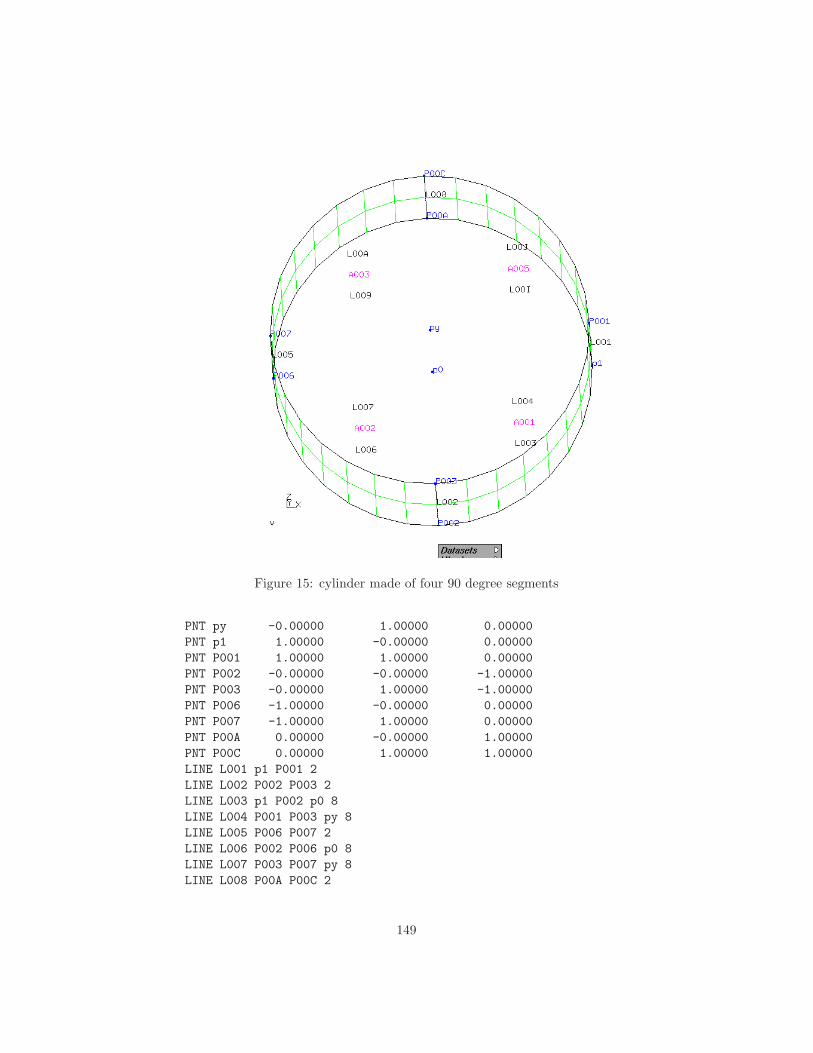
Figure 15: cylinder made of four 90 degree segments
PNT py -0.00000 1.00000 0.00000
PNT p1 1.00000 -0.00000 0.00000
PNT P001 1.00000 1.00000 0.00000
PNT P002 -0.00000 -0.00000 -1.00000
PNT P003 -0.00000 1.00000 -1.00000
PNT P006 -1.00000 -0.00000 0.00000
PNT P007 -1.00000 1.00000 0.00000
PNT P00A 0.00000 -0.00000 1.00000
PNT P00C 0.00000 1.00000 1.00000
LINE L001 p1 P001 2
LINE L002 P002 P003 2
LINE L003 p1 P002 p0 8
LINE L004 P001 P003 py 8
LINE L005 P006 P007 2
LINE L006 P002 P006 p0 8
LINE L007 P003 P007 py 8
LINE L008 P00A P00C 2
149
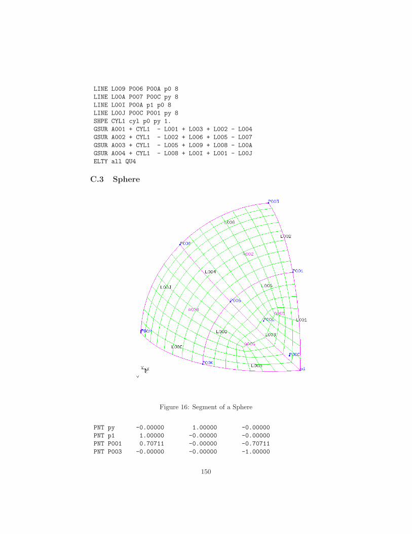
LINE L009 P006 P00A p0 8
LINE L00A P007 P00C py 8
LINE L00I P00A p1 p0 8
LINE L00J P00C P001 py 8
SHPE CYL1 cyl p0 py 1.
GSUR A001 + CYL1 - L001 + L003 + L002 - L004
GSUR A002 + CYL1 - L002 + L006 + L005 - L007
GSUR A003 + CYL1 - L005 + L009 + L008 - L00A
GSUR A004 + CYL1 - L008 + L00I + L001 - L00J
ELTY all QU4
C.3 Sphere
Figure 16: Segment of a Sphere
PNT py -0.00000 1.00000 -0.00000
PNT p1 1.00000 -0.00000 -0.00000
PNT P001 0.70711 -0.00000 -0.70711
PNT P003 -0.00000 -0.00000 -1.00000
150
PNT P006 0.70711 0.50000 -0.50000
PNT P008 -0.00000 0.70711 -0.70711
PNT P00C 0.70711 -0.00000 -0.00000
PNT P00K 0.70711 0.70711 -0.00000
PNT P00L -0.00000 -0.00000 -0.00000
PNT P00N -0.00000 1.00000 -0.00000
LINE L001 p1 P001 P00L 8
LINE L002 P001 P003 P00L 8
LINE L003 p1 P006 P00L 8
LINE L004 P006 P008 P00L 8
LINE L006 P001 P006 P00C 8
LINE L008 P003 P008 P00L 8
LINE L00A p1 P00K P00L 8
LINE L00C P00K P00N P00L 8
LINE L00G P006 P00K P00C 8
LINE L00J P008 P00N P00L 8
SHPE SPH1 sph P00L 1.
GSUR A005 + SPH1 - L003 + L001 + L006
GSUR A002 + SPH1 - L002 + L006 + L004 - L008
GSUR A006 + SPH1 + L003 + L00G - L00A
GSUR A004 + SPH1 - L004 + L00G + L00C - L00J
ELTY all QU4
C.4 Sphere (Volume)
PNT py 0.00000 1.00000 0.00000
PNT p1 1.00000 0.00000 0.00000
PNT P006 0.70711 0.50000 -0.50000
PNT P008 0.00000 0.70711 -0.70711
PNT P00C 0.70711 0.00000 0.00000
PNT P00K 0.70711 0.70711 0.00000
PNT P00L 0.00000 0.00000 0.00000
PNT P00N 0.00000 1.00000 0.00000
LINE L001 p1 P00L 8
LINE L002 P00L P008 8
LINE L003 p1 P006 P00L 8
LINE L004 P006 P008 P00L 8
LINE L005 P00L P00N 8
LINE L00A p1 P00K P00L 8
LINE L00C P00K P00N P00L 8
LINE L00G P006 P00K P00C 8
LINE L00J P008 P00N P00L 8
SHPE SPH1 sph P00L 1.
GSUR A001 + BLEND - L003 + L001 + L002 - L004
GSUR A002 + BLEND - L005 - L001 + L00A + L00C
GSUR A006 + SPH1 + L003 + L00G - L00A
151

Figure 17: Segment of a Sphere (Volume)
GSUR A004 + SPH1 - L004 + L00G + L00C - L00J
GSUR A003 + BLEND + L002 + L00J - L005
GBOD B001 NORM + A006 - A003 - A004 + A002 + A001
ELTY all HE20
C.5 Airfoil for cfd codes
All surfaces must be oriented in the same way. The sets are used to define areasfor the boundary conditions.
PNT P002 -0.24688 0.00667 0.00000
PNT P003 -0.24375 0.00903 0.00000
PNT P004 -0.23750 0.01228 0.00000
PNT P005 -0.23125 0.01450 0.00000
PNT P006 -0.22500 0.01608 0.00000
PNT P007 -0.21250 0.01798 0.00000
PNT P008 -0.20000 0.01875 0.00000
PNT P009 -0.18750 0.01900 0.00000
152

Figure 18: Airfoil for cfd codes
PNT P00A -0.17500 0.01888 0.00000
PNT P00C -0.15000 0.01785 0.00000
PNT P00E -0.12500 0.01602 0.00000
PNT P00G -0.10000 0.01368 0.00000
PNT P00I -0.07500 0.01090 0.00000
PNT P00J -0.05000 0.00770 0.00000
PNT P00K -0.02500 0.00420 0.00000
PNT P00L -0.01250 0.00230 0.00000
PNT P00O -0.25000 0.00000 0.00000
PNT P00P -0.24688 -0.00308 0.00000
PNT P00R -0.24375 -0.00427 0.00000
PNT P00S -0.23750 -0.00565 0.00000
PNT P00T -0.23125 -0.00653 0.00000
PNT P00V -0.22500 -0.00730 0.00000
PNT P00W -0.21250 -0.00875 0.00000
PNT P00X -0.20000 -0.00993 0.00000
PNT P00Z -0.18750 -0.01070 0.00000
153
PNT P010 -0.17500 -0.01115 0.00000
PNT P011 -0.15000 -0.01120 0.00000
PNT P012 -0.12500 -0.01043 0.00000
PNT P013 -0.10000 -0.00917 0.00000
PNT P014 -0.07500 -0.00750 0.00000
PNT P015 -0.05000 -0.00540 0.00000
PNT P016 -0.02500 -0.00308 0.00000
PNT P017 -0.01250 -0.00175 0.00000
PNT P019 0.00000 0.00000 0.00000
PNT P1 -0.50000 -0.50000 0.00000
PNT P2 0.50000 -0.50000 0.00000
PNT p3 0.50000 0.50000 0.00000
PNT p4 -0.50000 0.50000 0.00000
PNT P01A -0.18162 0.01898 0.00000
PNT P01B -0.18180 -0.01094 0.00000
PNT P046 -0.27025 0.01256 0.00000
PNT P059 -0.26599 0.28688 0.00000
PNT P049 -0.25144 0.02439 0.00000
PNT P05A -0.35589 0.17566 0.00000
PNT P04C -0.22636 0.03241 0.00000
PNT P04D -0.20128 0.03643 0.00000
PNT P05C -0.38027 0.00958 0.00000
PNT P04G -0.12604 0.03833 0.00000
PNT P04H -0.07588 0.03616 0.00000
PNT P04I -0.02572 0.03231 0.00000
PNT P05D -0.31932 -0.21136 0.00000
PNT P04L -0.27652 -0.00154 0.00000
PNT P04M -0.27025 -0.00803 0.00000
PNT P05F -0.20962 -0.27840 0.00000
PNT P04P -0.25373 -0.01567 0.00000
PNT P04R -0.22676 -0.02143 0.00000
PNT P04T -0.20124 -0.02394 0.00000
PNT P05G 0.01132 0.29145 0.00000
PNT P04W -0.12604 -0.02508 0.00000
PNT P04X -0.07588 -0.02519 0.00000
PNT P04Z -0.02572 -0.02355 0.00000
PNT P05H 0.00065 -0.30887 0.00000
PNT P052 -0.18074 0.03754 0.00000
PNT P054 -0.18133 -0.02465 0.00000
PNT P056 0.00118 0.02891 0.00000
PNT P058 0.00010 -0.02250 0.00000
PNT P05I 0.01244 0.50000 0.00000
PNT P05J 0.00610 -0.50000 0.00000
PNT P05L 0.50000 -0.34112 0.00000
PNT P05M 0.50000 0.29206 0.00000
PNT P05N 0.50000 0.05780 0.00000
154
PNT P05S 0.50000 -0.05314 0.00000
PNT P05V 0.50000 -0.00217 0.00000
PNT P00N -0.23448 0.01345 0.00000
PNT P02M -0.23471 -0.00608 0.00000
PNT P03B -0.24164 0.02804 0.00000
PNT P03C -0.23405 -0.02029 0.00000
PNT P03E -0.24536 0.00794 0.00000
PNT P03P -0.24464 -0.00400 0.00000
PNT pl1 -1.00000 0.00000 0.00000
PNT pl2 1.00000 0.00000 0.00000
SEQA S006 pnt P01A P00A P00C P00E P00G P00I P00J P00K P00L P019
SEQA S007 pnt P019 P017 P016 P015 P014 P013 P012 P011 P010 P01B
SEQA S00W pnt P03B P049 P046 P04L P04M P04P P03C
SEQA S00R pnt P052 P04G P04H P04I P056
SEQA S00S pnt P058 P04Z P04X P04W P054
SEQA S00T pnt P05F P05D P05C P05A P059
SEQA S001 pnt P01A P009 P008 P007 P006 P005 P00N
SEQA S00E pnt P03E P002 P00O P00P P03P
SEQA S00L pnt P052 P04D P04C P03B
SEQA S00A pnt P02M P00T P00V P00W P00X P00Z P01B
SEQA S00X pnt P03C P04R P04T P054
SEQA S002 pnt P00N P004 P003 P03E
SEQA S00P pnt P03P P00R P00S P02M
LINE L003 P01A P052 910
LINE L00C P01A P019 S006 120
LINE L00E P019 P01B S007 120
LINE L004 p4 P1 150
LINE L05F P2 P05L -204
LINE L05S P05L P05S -912
LINE L05C P1 P05J 120
LINE L006 P01B P054 910
LINE L007 P019 P056 910
LINE L008 P058 P019 -910
LINE L00G P05S P05V -210
LINE L00N P03B P03C S00W 130
LINE L03R P052 P056 S00R 120
LINE L00I P05V P05N 210
LINE L03S P058 P054 S00S 120
LINE L04V p4 P059 -204
LINE L04W P059 P052 -912
LINE L04X P054 P05F 912
LINE L04Z P05F P1 204
LINE L050 P05F P059 S00T 150
LINE L052 P059 P05G 120
LINE L054 P05F P05H 120
LINE L056 P05H P058 -912
155

LINE L058 P056 P05G 912
LINE L059 p3 P05I 130
LINE L05A P05I p4 120
LINE L05D P05J P2 130
LINE L05V P056 P05N 130
LINE L05I P05M p3 204
LINE L05L P05N P05M 912
LINE L05Z P058 P05S 130
LINE L06C P019 P05V 130
LINE L06F P05M P05G 130
LINE L06H P05G P05I 204
LINE L06I P05L P05H 130
LINE L06J P05H P05J 204
LINE L001 P01A P00N S001 -210
LINE L00A P03E P03P S00E 120
LINE L00K P052 P03B S00L 110
LINE L009 P02M P01B S00A 210
LINE L00O P03C P054 S00X 110
LINE L002 P00N P03E S002 -205
LINE L00L P03P P02M S00P 205
LINE cl pl1 pl2 120
LINE L005 P00O P019 120
LCMB C001 + L001 + L002 + L00A + L00L + L009
LCMB C004 + L00K + L00N + L00O
GSUR A001 + BLEND + L003 + C004 - L006 - C001
GSUR A002 + BLEND + L006 - L03S + L008 + L00E
GSUR A003 + BLEND + L00C + L007 - L03R - L003
GSUR A004 + BLEND - L008 + L05Z + L00G - L06C
GSUR A005 + BLEND + L06C + L00I - L05V - L007
GSUR A00I + BLEND - L04W - L050 - L04X - C004
GSUR A00J + BLEND - L04V + L004 - L04Z + L050
GSUR A00K + BLEND + L04Z + L05C - L06J - L054
GSUR A00L + BLEND + L06J + L05D + L05F + L06I
GSUR A00N + BLEND + L04V + L052 + L06H + L05A
GSUR A00O + BLEND - L06H - L06F + L05I + L059
GSUR A00P + BLEND + L04W + L03R + L058 - L052
GSUR A00R + BLEND + L04X + L054 + L056 + L03S
GSUR A00S + BLEND - L058 + L05V + L05L + L06F
GSUR A00T + BLEND - L056 - L06I + L05S - L05Z
SETA wall l L05C
SETA wall l L059
SETA wall l L05A
SETA wall l L05D
SETA profil l L00C
SETA profil l L00E
SETA profil l L001
156
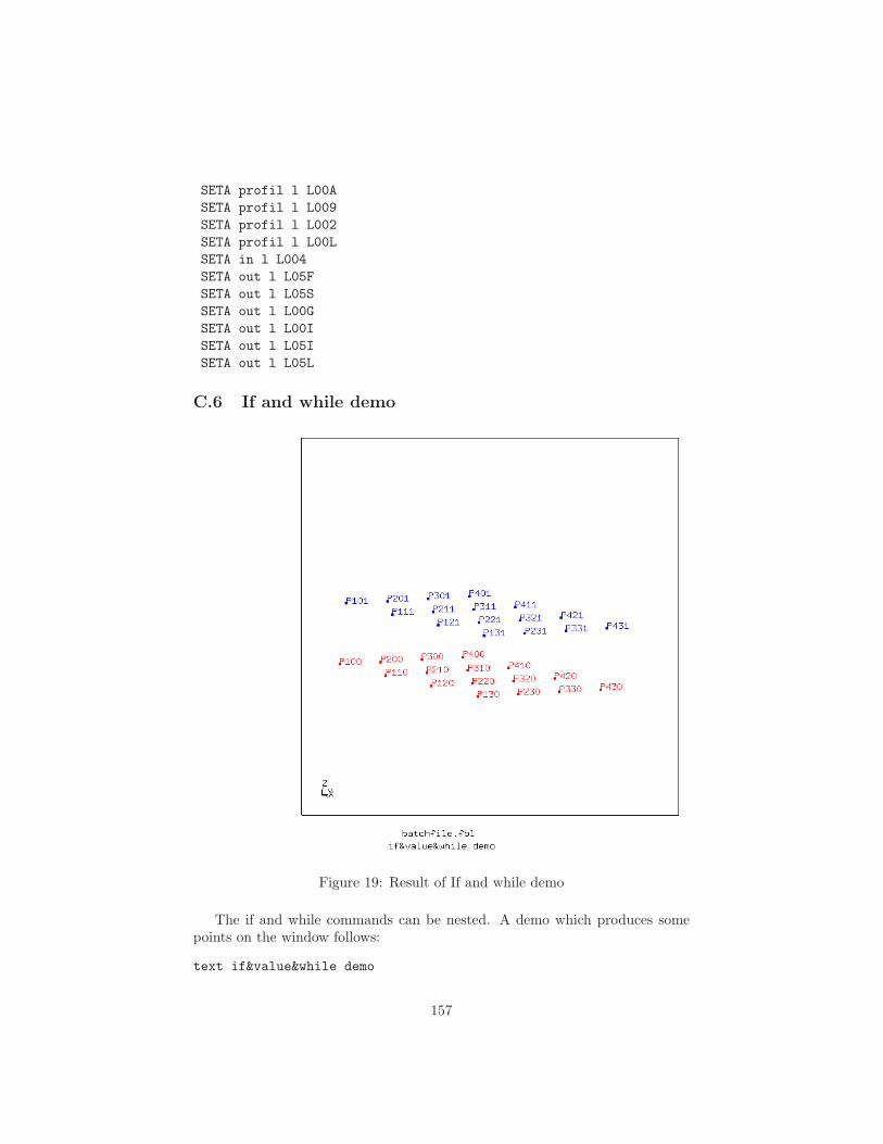
SETA profil l L00A
SETA profil l L009
SETA profil l L002
SETA profil l L00L
SETA in l L004
SETA out l L05F
SETA out l L05S
SETA out l L00G
SETA out l L00I
SETA out l L05I
SETA out l L05L
C.6 If and while demo
Figure 19: Result of If and while demo
The if and while commands can be nested. A demo which produces somepoints on the window follows:
text if&value&while demo
157

# def the leading letter of point names
valu vp P
# define the initial x value
valu vx 0.
# define parameters
valu v2 4
valu v3 1
# start loop:
while vx < v2
valu vy 0.
valu vz 0.
seto S1
while vy < v2
# define the pnt coordinates
valu vy + vy v3
valu vy int vy
valu vx int vx
valu vz int vz
# define the pnt name
valu p1 & vp vy
valu p1 & p1 vx
valu p1 & p1 vz
# generate the pnt
pnt p1 vx vy vz
endwhile
setc
valu vy 0.
valu vz 1.
seto S2
while vy < v2
valu vy + vy v3
valu vy int vy
valu vx int vx
valu vz int vz
valu p2 & vp vy
valu p2 & p2 vx
valu p2 & p2 vz
pnt p2 vx vy vz
endwhile
setc
valu vx + vx v3
if vx == 1
plot pa S1 r
else
plus pa S2 b
endif
158

endwhile
send all fbd
# demo on how to write the content of variables to writedemo.txt
valu vx int vx
valu vy int vy
sys echo VX: vx VY: vx VZ: vz >| writedemo.txt
References
[1] OpenGL-Like Rendering Toolkit, from Brian Paul,http://www.mesa3d.org/
[2] OpenGL Utility Toolkit (GLUT), from Mark J. Kilgard
[3] CalculiX GraphiX (cgx), from Klaus Wittig, [email protected]
[4] NETGEN, unstructured mesher, http://www.hpfem.jku.at/netgen/
[5] dolfyn, Open Source CFD code, http://www.dolfyn.net
[6] Duns, a two- and three dimensional cfd code,http://sourceforge.net/projects/duns/
[7] ISAAC, a two- and three dimensional cfd code, http://isaac-cfd.sourceforge.net
[8] OpenFOAM, a three dimensional cfd code, http://www.opencfd.co.uk
[9] Tochnog, a free fem-code, http://tochnog.sourceforge.net/
[10] Tutorial for CalculiX, from Dr. Guido Dhondt,http://www.dhondt.de/tutorial.html
[11] ImageMagick 5.1.0 00/01/01 Q:8 [email protected]. Copy-right: Copyright (C) 2000 ImageMagick Studio
[12] Mozilla Foundation, http://www.firefox.com
[13] S. A. Coons, ’Surfaces for computer-aided design of space forms’. ProjectMAC, MIT (1964). Revised to MAC-TR-41 (1967).
[14] mesh2d, unstructured 2D-mesher from B. Kaan Karamete, Ph.D, No URLAvailable
[15] Paul Dierckx, Curve and Surface Fitting with Splines, Oxford. UniversityPress, 1993
159


![Βίντεο για εκμάθηση Scratch 1€¦ · Φύλλα εργασίας για εκμάθηση Scratch 1͙4 – Κοκκόρη Αθηνά [3] Εφαρογή σο Scratch:](https://static.fdocuments.us/doc/165x107/5fa1e23ac073f719dc091d73/-f-scratch-1-f-.jpg)