CALCULATION OF THE SHIELDING EFFECTIVENESS OF … CARBON-FIBER COMPOSITE STRUCTURES Mohammadali...
91
CALCULATION OF THE SHIELDING EFFECTIVENESS OF CARBON-FIBER COMPOSITE STRUCTURES Mohammadali Ansarizadeh A Thesis in The Department of Electrical and Computer Engineering Presented in Partial Fulfillment of the Requirements for the Degree of Master of Applied Science Concordia University Montreal, Quebec, Canada September 2013 c Mohammadali Ansarizadeh, 2013
-
Upload
truongtuong -
Category
Documents
-
view
224 -
download
1
Transcript of CALCULATION OF THE SHIELDING EFFECTIVENESS OF … CARBON-FIBER COMPOSITE STRUCTURES Mohammadali...
CALCULATION OF THE SHIELDING EFFECTIVENESS
OF CARBON-FIBER COMPOSITE STRUCTURES
Mohammadali Ansarizadeh
A Thesis
in
The Department
of
Electrical and Computer Engineering
Presented in Partial Fulfillment of the Requirements
for the Degree of Master of Applied Science
Concordia University
Montreal, Quebec, Canada
September 2013
c©Mohammadali Ansarizadeh, 2013

Abstract
Calculation of the Shielding Effectiveness of Carbon-Fiber Composite
Structures
Mohammadali Ansarizadeh
Carbon-fiber composite (CFC) materials are replacing metals in the construction of
modern aircraft because of their outstanding strength/weight ratio. The purpose of
this thesis is to identify the capabilities and limitations of the commercially available
software in calculating the shielding effectiveness (SE) of CFC structures. This work
is started by a literature survey focused on the characterization and modeling of CFC
panels.
The homogenized model of CFC panels is analyzed using the skin-effect approxi-
mation in a method of moments (MoM) solution. It is found that the stack-to-sheet
conversion is a limiting factor in the skin effect approximation and not the homoge-
nization scheme.
Experimental results are presented which indicate that performance of monopole
antennas up to a frequency of 12.5 GHz is not altered by replacing a metallic ground
plane with a CFC one. Also, a monopole antenna is mounted on hollow CFC and
aluminum cubes with the same physical dimensions and the radiated electromagnetic
interference (EMI) inside the cube are theoretically compared.
Although wire meshes with unbonded junctions are better shields it is shown
that this is less important for meshes is epoxy as compared to free space. For CFC
materials reinforced with woven carbon-fiber fabrics the effects of physical contact
between orthogonally oriented fiber bundles are examined. It is found that bonding
CFC fiber bundles at the junctions actually improves the shielding performance.
The simulation results for the electric and magnetic SE inside a hollow spherical
CFC shell are compared with the benchmark analytic solutions. It is shown that the
analytic solutions could not be numerically evaluated unless the wave functions are
iii

expressed in terms of the thickness of CFC materials.
iv

Acknowledgements
I would like to thank my supervisor Prof. Robert Paknys for his academic and
financial support. This work would not have been possible without his support and
supervision. I am grateful to Prof. Sebak and Dr. Alper Ozturk for their supervision
in the early stages of my research. I appreciate Prof. Laurin for providing me access
with the measurement setup at Ecole Polytechnique de Montreal and, also, valuable
feedback about my work. I thank Prof. Kishk for answering some of my questions.
Support from the National Science and Engineering Research Council (NSERC)
CRD Program, the Consortium de Recherche et d’Innovation en Aerospatiale au
Quebec (CRIAQ) and industry partners Bombardier Aerospace and MacDonald Det-
twiler and Associates Inc. is gratefully acknowledged.
I appreciate Shailesh Prasad, Dr. Donald Davis and my good friends and col-
leagues Ali Chakavak, Ayman, Zouhair, Tiago Leao, Mohamed Hassan, and Mehdi
Ardavan. Last but not least, I thank my parents for their support and sacrifices.
v
Contents
1 Literature Survey 1
1.1 Introduction . . . . . . . . . . . . . . . . . . . . . . . . . . . . . . . . 1
1.2 Overview of the Pioneering Research . . . . . . . . . . . . . . . . . . 2
1.3 Basic Assumptions . . . . . . . . . . . . . . . . . . . . . . . . . . . . 3
1.4 Thesis Outline . . . . . . . . . . . . . . . . . . . . . . . . . . . . . . . 4
2 The Skin-Effect Approximation 6
2.1 Introduction . . . . . . . . . . . . . . . . . . . . . . . . . . . . . . . . 6
2.2 Homogenization of a CFC Laminate . . . . . . . . . . . . . . . . . . . 7
2.3 Tensor Permittivity of Embedded Fibers . . . . . . . . . . . . . . . . 8
2.4 The Skin-Effect Approximation . . . . . . . . . . . . . . . . . . . . . 9
2.5 Stack-to-Sheet Conversion . . . . . . . . . . . . . . . . . . . . . . . . 10
2.6 Numerical Results . . . . . . . . . . . . . . . . . . . . . . . . . . . . . 12
2.6.1 A Single CFC Laminate . . . . . . . . . . . . . . . . . . . . . 12
2.6.2 CFC Panel with Two Laminates . . . . . . . . . . . . . . . . . 13
2.6.3 CFC Panel with Four Laminates . . . . . . . . . . . . . . . . 15
2.6.4 Hollow Cubic Shell with a CFC Face . . . . . . . . . . . . . . 17
2.7 Conclusions . . . . . . . . . . . . . . . . . . . . . . . . . . . . . . . . 19
3 Monopole Antennas on CFC Structures 21
3.1 Introduction . . . . . . . . . . . . . . . . . . . . . . . . . . . . . . . . 21
3.2 Monopole Antennas on CFC Ground Planes . . . . . . . . . . . . . . 22
vi

3.3 Interference Due to VHF Antennas . . . . . . . . . . . . . . . . . . . 25
3.4 Interference Due to HF Antennas . . . . . . . . . . . . . . . . . . . . 28
3.5 Conclusions . . . . . . . . . . . . . . . . . . . . . . . . . . . . . . . . 30
4 Effects of Interlaminar Bondings 31
4.1 Introduction . . . . . . . . . . . . . . . . . . . . . . . . . . . . . . . . 31
4.2 Wire Meshes in Free Space . . . . . . . . . . . . . . . . . . . . . . . . 32
4.3 Wire Meshes Embedded in Epoxy . . . . . . . . . . . . . . . . . . . . 35
4.4 Woven Reinforcements . . . . . . . . . . . . . . . . . . . . . . . . . . 38
4.5 1D-Array Reinforcement . . . . . . . . . . . . . . . . . . . . . . . . . 40
4.6 2D-Bonded and Unbonded Reinforcements . . . . . . . . . . . . . . . 41
4.7 Conclusions . . . . . . . . . . . . . . . . . . . . . . . . . . . . . . . . 43
5 Shielding Effectiveness of CFC Enclosures 44
5.1 Introduction . . . . . . . . . . . . . . . . . . . . . . . . . . . . . . . . 44
5.2 The Inside-Outside SIE Formulation . . . . . . . . . . . . . . . . . . 45
5.3 SE of an Infinite CFC Panel . . . . . . . . . . . . . . . . . . . . . . . 47
5.4 SE Inside a Hollow CFC Shell . . . . . . . . . . . . . . . . . . . . . . 49
5.5 Conclusions . . . . . . . . . . . . . . . . . . . . . . . . . . . . . . . . 52
6 Conclusions and Future Work 54
6.1 Conclusions . . . . . . . . . . . . . . . . . . . . . . . . . . . . . . . . 54
6.2 Future Work . . . . . . . . . . . . . . . . . . . . . . . . . . . . . . . . 58
A SE Inside a Hollow Spherical CFC Shell 65
A.1 Formulating the Problem . . . . . . . . . . . . . . . . . . . . . . . . . 65
A.2 Fields at the Origin . . . . . . . . . . . . . . . . . . . . . . . . . . . . 73
A.3 Numerical Issues . . . . . . . . . . . . . . . . . . . . . . . . . . . . . 73
vii

List of Figures
2.1 (a) and (b) are, respectively, the idealized geometry of a CFC laminate
and its equivalent layer model [1]. . . . . . . . . . . . . . . . . . . . . 8
2.2 The geometry of the ideal model of a CFC laminate. D, P, and L
are, respectively, the fiber diameter, periodicity of the fiber array, and
laminate thickness. εm = 2ε0 is the permittivity of the binding dielec-
tric material. εf = 2ε0 and σf = 104 S/m are the permittivity and
conductivity of the fibers, respectively. . . . . . . . . . . . . . . . . . 12
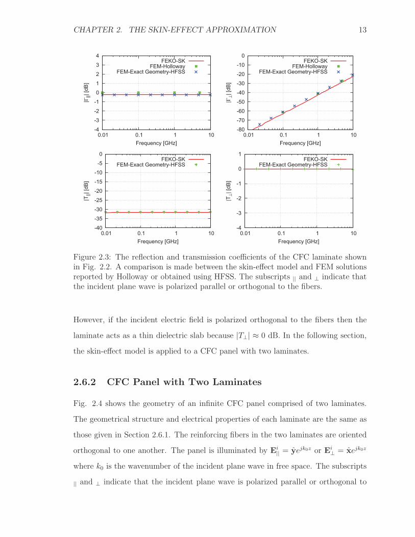
2.3 The reflection and transmission coefficients of the CFC laminate shown
in Fig. 2.2. A comparison is made between the skin-effect model and
FEM solutions reported by Holloway or obtained using HFSS. The
subscripts || and ⊥ indicate that the incident plane wave is polarized
parallel or orthogonal to the fibers. . . . . . . . . . . . . . . . . . . . 13
2.4 The geometry of a CFC panel with two laminates. The reinforcing
fibers are oriented along the y- and x-axis. The geometrical and elec-
trical parameters of each laminate are given in Section 2.6.1. . . . . . 14
2.5 The reflection and transmission coefficients of a CFC panel with two
laminates for a normally incident plane wave. The panel is illuminated
by a normally incident plane wave polarized along the x- and y-axis. . 14
2.6 The geometry of a CFC panel comprised of four laminates. The lam-
inates have the same geometrical and electrical properties as the one
discussed in Section 2.6.1. . . . . . . . . . . . . . . . . . . . . . . . . 16
viii
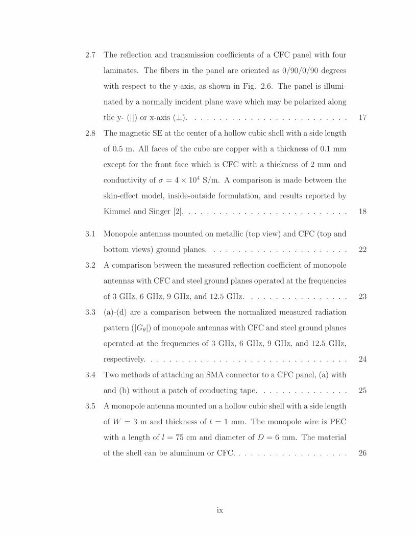
2.7 The reflection and transmission coefficients of a CFC panel with four
laminates. The fibers in the panel are oriented as 0/90/0/90 degrees
with respect to the y-axis, as shown in Fig. 2.6. The panel is illumi-
nated by a normally incident plane wave which may be polarized along
the y- (||) or x-axis (⊥). . . . . . . . . . . . . . . . . . . . . . . . . . 17
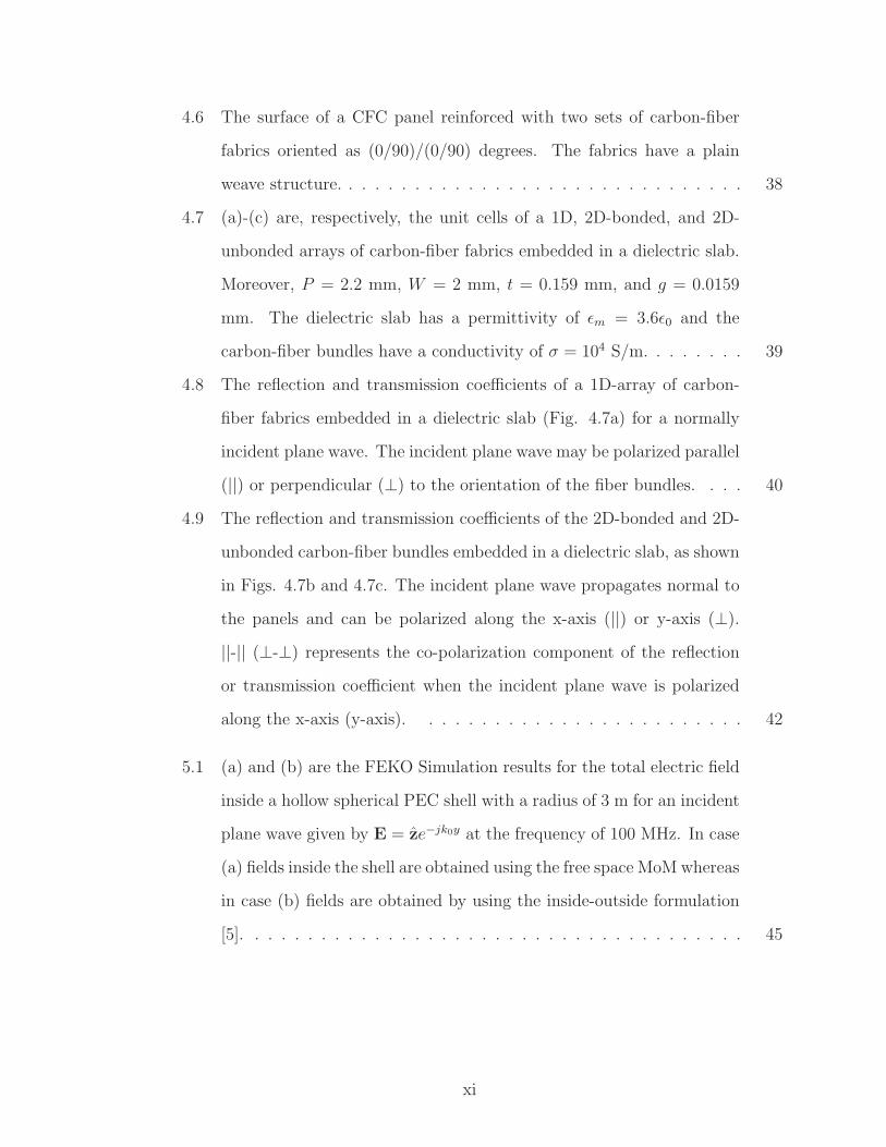
2.8 The magnetic SE at the center of a hollow cubic shell with a side length
of 0.5 m. All faces of the cube are copper with a thickness of 0.1 mm
except for the front face which is CFC with a thickness of 2 mm and
conductivity of σ = 4 × 10⁴ S/m. A comparison is made between the
skin-effect model, inside-outside formulation, and results reported by
Kimmel and Singer [2]. . . . . . . . . . . . . . . . . . . . . . . . . . . 18
3.1 Monopole antennas mounted on metallic (top view) and CFC (top and
bottom views) ground planes. . . . . . . . . . . . . . . . . . . . . . . 22
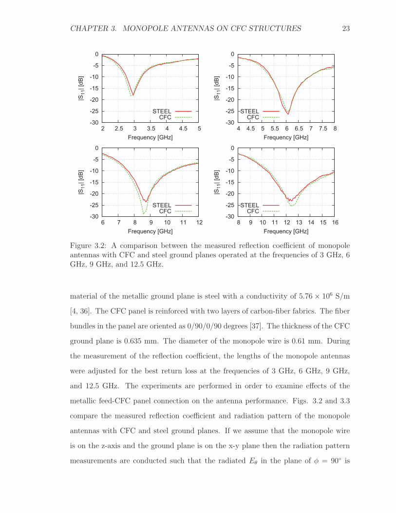
3.2 A comparison between the measured reflection coefficient of monopole
antennas with CFC and steel ground planes operated at the frequencies
of 3 GHz, 6 GHz, 9 GHz, and 12.5 GHz. . . . . . . . . . . . . . . . . 23
3.3 (a)-(d) are a comparison between the normalized measured radiation
pattern (|Gθ|) of monopole antennas with CFC and steel ground planes
operated at the frequencies of 3 GHz, 6 GHz, 9 GHz, and 12.5 GHz,
respectively. . . . . . . . . . . . . . . . . . . . . . . . . . . . . . . . . 24
3.4 Two methods of attaching an SMA connector to a CFC panel, (a) with
and (b) without a patch of conducting tape. . . . . . . . . . . . . . . 25
3.5 A monopole antenna mounted on a hollow cubic shell with a side length
of W = 3 m and thickness of t = 1 mm. The monopole wire is PEC
with a length of l = 75 cm and diameter of D = 6 mm. The material
of the shell can be aluminum or CFC. . . . . . . . . . . . . . . . . . . 26
ix

3.6 (a)-(d) are the electric and magnetic fields on the y-z plane inside the
hollow cubic shell shown in Fig. 3.5. The average power delivered to
the monopole antenna is 1 W of at the frequency of 100 MHz. . . . . 27
3.7 The electric and magnetic fields on the y-z plane inside the hollow cubic
shell shown in Fig. 3.5. The average power delivered to the monopole
is delivered 1 W of at the frequency of 3 MHz. . . . . . . . . . . . . . 29
4.1 The geometry of the unit cells of bonded and unbonded PEC wire
meshes in free space. D, P , and S are, respectively, the wire diameter,
periodicity of the mesh, and vertical spacing between wire arrays. . . 32
4.2 A comparison between FEKO simulation and results of Hill and Wait
[3] for the co-polarization and cross-polarization transmission coeffi-
cients of bonded and unbonded PEC thin wire meshes in free space
versus the azimuth angle φ. . . . . . . . . . . . . . . . . . . . . . . . 33
4.3 The co- and cross-polarization reflection and transmission coefficients
of bonded and unbonded wire meshes in free space (Fig. 4.1) versus
the azimuth angle φ for an oblique incident plane wave with θ = 70◦
at a frequency where P = λ0/100. . . . . . . . . . . . . . . . . . . . . 34
4.4 The geometry of the bonded and unbonded wire meshes embedded in
an infinite dielectric epoxy slab. The thickness of the dielectric slab is
L = 4D. D, P , and S are, respectively, the wire diameter, periodicity
of the mesh, and vertical spacing between wire arrays. The wires are
assumed to be PEC and the permittivity of the dielectric slab is epoxy
with εm = 3.6ε0 [4]. . . . . . . . . . . . . . . . . . . . . . . . . . . . . 36
4.5 (a)-(h) are the co- and cross-polarization reflection and transmission
coefficients of bonded and unbonded wire meshes embedded in an in-
finite epoxy slab versus the azimuth angle φ at an oblique incidence
angle of θ = 70◦. Two frequencies are chosen such that P = 0.01λ0
and P = 0.25λ0. . . . . . . . . . . . . . . . . . . . . . . . . . . . . . . 37
x
4.6 The surface of a CFC panel reinforced with two sets of carbon-fiber
fabrics oriented as (0/90)/(0/90) degrees. The fabrics have a plain
weave structure. . . . . . . . . . . . . . . . . . . . . . . . . . . . . . . 38
4.7 (a)-(c) are, respectively, the unit cells of a 1D, 2D-bonded, and 2D-
unbonded arrays of carbon-fiber fabrics embedded in a dielectric slab.
Moreover, P = 2.2 mm, W = 2 mm, t = 0.159 mm, and g = 0.0159
mm. The dielectric slab has a permittivity of εm = 3.6ε0 and the
carbon-fiber bundles have a conductivity of σ = 104 S/m. . . . . . . . 39
4.8 The reflection and transmission coefficients of a 1D-array of carbon-
fiber fabrics embedded in a dielectric slab (Fig. 4.7a) for a normally
incident plane wave. The incident plane wave may be polarized parallel
(||) or perpendicular (⊥) to the orientation of the fiber bundles. . . . 40
4.9 The reflection and transmission coefficients of the 2D-bonded and 2D-
unbonded carbon-fiber bundles embedded in a dielectric slab, as shown
in Figs. 4.7b and 4.7c. The incident plane wave propagates normal to
the panels and can be polarized along the x-axis (||) or y-axis (⊥).
||-|| (⊥-⊥) represents the co-polarization component of the reflection
or transmission coefficient when the incident plane wave is polarized
along the x-axis (y-axis). . . . . . . . . . . . . . . . . . . . . . . . . 42
5.1 (a) and (b) are the FEKO Simulation results for the total electric field
inside a hollow spherical PEC shell with a radius of 3 m for an incident
plane wave given by E = ze−jk0y at the frequency of 100 MHz. In case
(a) fields inside the shell are obtained using the free space MoM whereas
in case (b) fields are obtained by using the inside-outside formulation
[5]. . . . . . . . . . . . . . . . . . . . . . . . . . . . . . . . . . . . . . 45
xi

xii
5.2 (a) The geometry of the unit cell of an infinite CFC panel modeled as
a dielectric material with σ = 104 S/m. The panel thickness is 0.159
mm. The triangle edge length (TEL) denotes the mesh size in FEKO.
TEL is expressed in terms of the wavelength in the CFC panel. (b) The
transmission coefficient of the panel shown in Fig. 5.2a for a normally
incident plane wave. The incident plane wave is polarized along the
x-axis and its frequency varies from 1 GHz to 20 GHz. . . . . . . . . 47
5.3 The analytic and simulation results for the electric and normalized
magnetic fields at the center of a hollow spherical CFC shell with a
radius of 3 m, thickness of 1 mm, and conductivity of σ = 104 S/m.
The incident plane wave is Ei = xe−jk0z. . . . . . . . . . . . . . . . . 50
5.4 The analytic and simulation results for the electric and magnetic fields
on the z-axis inside a hollow spherical CFC shell with a radius of 3 m,
thickness of 1 mm, and conductivity of σ = 104 S/m. The incident
plane wave is Ei = xe−jk0z where k0 is wavenumber of the incident
plane wave at the frequencies of 43.672 MHz and 71.508 MHz. . . . . 51
A.1 The cross section of a hollow spherical CFC shell which is illuminated
by a plane wave. a and b represent the inner and outer radii of the
shell, respectively. The subscripts 1, 2, and 3, respectively, represent
the regions corresponding to r ≤ a, a ≤ r ≤ b, and r ≥ b. . . . . . . . 66

List of Symbols and Acronyms
β0 Propagation constant in free space
δs Skin depth
ε0 Permittivity of free space
εm Permittivity of epoxy
εr Relative permittivity
η0 Impedance of free space
λ Material wavelength
μ0 Permeability of free space
σ Conductivity
c0 Speed of light in free space
k0 Wavenumber in free space
Zs Equivalent sheet impedance
Js Equivalent electric surface current
E Electric field
H Magnetic field
CFC Carbon-Fiber Composite
xiii

xiv
EM Electromagnetics
EMC Electromagnetic Compatibility
EMI Electromagnetic Interference
FEKO FEldberechnung bei Korpern mit beliebiger Oberflache, meaning, Field com-
putations involving bodies of arbitrary shape
FIT Finite Integration Technique
HFSS High Frequency Structural Simulator
MoM Method of Moments
PEC Perfect Electric Conductor
PMCHWT Poggio Miller Chang Harrington Wu Tsai
RCS Radar Cross Section
SE Shielding Effectiveness
SEL Segment Edge Length
SEP Surface Equivalence Principle
SIE Surface Integral Equations
TEL Triangle Edge Length
UHF Ultra High Frequency
VEP Volume Equivalence Principle
VHF Very High Frequency

Chapter 1
Literature Survey
1.1 Introduction
There is a growing trend in the aerospace industries to replace metals with carbon-
fiber composite (CFC) materials because they offer superior mechanical performances
at a lower cost [6]. In fact, the Bombardier aerospace company is using CFC ma-
terials in the construction of its modern aircraft. CFC panels are synthesized as a
sandwich of multiple laminates. A laminate is often composed of a planar array of
long continuous carbon-fibers embedded in an epoxy host medium. A single lami-
nate is strongly anisotropic. However, by progressively changing the orientation of
the reinforcing carbon-fibers in a CFC panel, bulk isotropic mechanical and electri-
cal material properties may be obtained. The anisotropic conductivity of a single
CFC laminate is not of interest in this thesis because CFC panels with industrial
applications are usually quasi-isotropic which are modeled as isotropic conducting
materials with a conductivity in the order of 104 S/m [7]. In fact, the conductivity
of CFC materials is almost 1000 times lower than the conductivity of most metals.
Since conductivity plays an important role in SE, the EMC may be compromised by
replacing metals with CFC materials. Therefore, it is necessary to understand the
capabilities and limitations of the commercially available software while calculating
1

CHAPTER 1. LITERATURE SURVEY 2
the SE of CFC structures so that the design engineer can assure if a CFC substitute
will meet the required standards. FEKO offers a MoM solver for SE problems in-
volving CFC materials. The purpose of this thesis is to understand the capabilities
and limitations of an MoM SIE formulation in calculating the SE of CFC structures.
This formulation is conveniently available in the commercial EM solver code FEKO
[8].
To understand the research history on the EM properties of CFC materials, a brief
literature survey on characterization and modeling of CFC materials is presented in
the following section.
1.2 Overview of the Pioneering Research
To our knowledge, the earliest EM study of CFC materials dates back to 1971 which
was focused on the homogenized conductivity of a single laminate [9]. Later in
1972, a series of destructive and nondestructive experiments focused on the effects of
lightning-produced currents on CFC panels were reported [10]. Knibbs and Morris
modeled a CFC laminate from the knowledge of its mechanical, thermal, and elec-
trical properties [11]. Their model was based on fibers embedded in a dielectric host
medium. It was concluded that fibers in a CFC laminate do not have exactly the
same orientation and there is misalignment from the nominal orientation. Moreover,
there are fiber-to-fiber electrical contacts in a laminate which are only 25% effective
[11]. In 1975, Keen tested a CFC reflector antenna and reported that at X-band
frequencies if the surface of a CFC reflector is not covered with a metallic coating
then a gain loss of 0.5 dB is incurred [12]. Later, Keen pointed out that the surface
roughness is the main cause of the gain loss and not the relatively lower conductiv-
ity of CFC materials [13]. According to Blake, the difference between the gain and
radiation pattern of UHF antennas mounted on metallic and CFC ground planes is
“little”. However, the magnetic SE of CFC materials is reported as “minimal” [14].
CHAPTER 1. LITERATURE SURVEY 3
Casey in 1977, calculated the SE of CFC panels by using boundary conditions that
relate the tangential electric and magnetic fields on both sides of a laminate [15].
Casey noted that quasi-isotropic CFC panels can be modeled as isotropic conducting
materials with a conductivity in the order of 104 S/m. Weinstock studied the impact
of replacing metals with CFC panels in the construction of aircraft [16]. One of his
conclusions was that the main reasons for the reduction of SE in CFC enclosures are
the discontinuity of the surface currents at seams and joints.
Hill and Wait calculated the reflection and transmission coefficients of wire meshes
in free space and reported that unbonded wire meshes are superior EM shields com-
pared to the bonded case [17]. Holloway et al. proposed equivalent-layer models to
simplify analysis of CFC panels [1]. In their model, the electrical contact between
fibers in the same laminate or in adjacent laminates were ignored. Kazerani used
FEKO to obtain the radiation pattern of antennas that are mounted on a CFC air-
craft fuselage [18]. Mehdipour used the equivalent-layer models of Holloway et al. to
calculate the SE of CFC materials [19]. Furthermore, Mehdipour et al. showed that
carbon-fiber nanotubes may be used to increase the conductivity of CFC materials
[20].
Due to a limited current handling capability, CFC materials are damaged by
high electric currents associated with lightning strikes. Therefore, a series of lighting
protection schemes for CFC materials have been developed [21].
1.3 Basic Assumptions
This work is focused on calculating the SE of CFC structures using the commercially
available software FEKO [8]. We will focus on the surface integral equations (SIE)
and method of moments (MoM) solver in FEKO. Throughout this thesis, the term
“CFC laminate” is referred to a dielectric slab reinforced with long continuous parallel
carbon-fiber reinforcements. If there is only one laminate then the reinforcing fibers

CHAPTER 1. LITERATURE SURVEY 4
are equally spaced and non-touching but in practice not all fibers are parallel and there
is misalignment between the fibers. Moreover, there is electrical contact between the
reinforcing fibers in a CFC panel. The term “panel” refers to a material whose
width and length are much larger than its thickness. The term “CFC panel” refers
to the sandwich structure of woven fibers forming multiple CFC laminates. In this
thesis, CFC panels with quasi-isotropic material properties are modeled as isotropic
conducting materials with σ = 104 S/m unless otherwise stated [22]. Furthermore,
simulation or analytic results that differ by less than 3 dB are considered to be in
good agreement with one another.
1.4 Thesis Outline
The thesis is organized as follows. In Chapter 2, the skin-effect approximation is
used in a MoM solver to calculate the reflection and transmission coefficients of CFC
panels and the results are compared with Holloway et al. [1]. Application of the skin-
effect model is motivated by a FEKO application note in which CFC panels were
modeled using the skin-effect approximation [23]. In Chapter 3, effects of replacing
metallic structures with CFC ones on the reflection coefficient, radiation pattern,
or radiated electromagnetic interference (EMI) of monopole antennas are examined.
Experimental and simulation results will be reported. This chapter is motivated
by the fact that in modern aircraft, monopole antennas are being mounted on a
CFC rather than a metallic fuselage. Chapter 4 is focused on the effects of bonding
between orthogonally oriented reinforcements in adjacent laminates. The reinforcing
fibers in the CFC panels that were analyzed by Holloway et al. were unbonded while
some CFC panels have a woven structure with physical contact between orthogonally
oriented reinforcements. The bonding between orthogonally oriented wires can affect
the reflection and transmission coefficient of wire meshes [17, 24, 25, 26]. That is
why in Chapter 4, effects of interlaminar bondings on the reflection and transmission

CHAPTER 1. LITERATURE SURVEY 5
coefficients of CFC panels are investigated. Chapter 5 is focused on the electric
and magnetic SE of CFC enclosures. Certain benchmark solutions are developed to
validate the FEKO simulation results. Numerical difficulties were encountered while
evaluating the benchmark SE quantities. In Appendix A, an approach is presented
to resolve such numerical problems. Finally, conclusions and suggestions for future
work are presented in Chapter 6.

Chapter 2
The Skin-Effect Approximation
2.1 Introduction
An ideal model of a CFC laminate is a dielectric slab reinforced by an array of
long continuous carbon-fibers. In each laminate, carbon-fibers are assumed to be
parallel, equally spaced, and not in contact with one another. CFC panels are usually
composed of a stack of multiple laminates where in each laminate carbon-fibers have
a specific orientation. By changing the orientation of the reinforcing fibers through
the panel, quasi-isotropic mechanical and electrical properties are obtained. The
diameter of individual carbon-fibers and the spacing between the fibers are in the
order of micrometers. However, frequency bands that are used in navigation and
communication systems correspond to wavelengths that are much larger than the
geometrical periodicity of CFC materials. As a result, CFC panels can be replaced
with equivalent homogeneous models because it is not necessary to calculate surface
or volume currents for individual carbon-fibers. Consequently, the EM analyses of
CFC materials is greatly simplified.
In order to analyze CFC materials in FEKO it is recommended that the skin-effect
model (“SK-card”) be used [23]. This approach is motivated by a FEKO application
note in which the skin-effect model is used to calculate the RCS of aircraft with a
6
CHAPTER 2. THE SKIN-EFFECT APPROXIMATION 7
CFC skin [23, 27]. The FEKO skin-effect model is based on approximate boundary
conditions and calculates the electric surface currents on CFC materials. The FEKO
skin-effect model can be used to analyze CFC panels composed of a single or multiple
laminates. The main purpose of this chapter is to examine FEKO’s ability to calculate
the EM SE of CFC panels. The geometrical and constitutive parameters of the
panels under consideration are the same as those used by Holloway et al. so that a
comparison can be made between published results and FEKO simulations.
This chapter is organized as follows. In the next section, a CFC laminate is
modeled with an equivalent-layer model composed of three homogeneous layers. Cal-
culation of the homogenized complex tensor permittivity of fibers embedded in a
dielectric slab is discussed in Section 2.3. In Section 2.4, the skin-effect approxima-
tion in FEKO is briefly explained. Then in Section 2.5, the multilayer structure CFC
panels is shrunk to a sheet with zero thickness. Next in Section 2.6, the simulation
results for the reflection and transmission coefficients of CFC panels composed of
one, two, and four laminates are presented and compared with published literature
[1]. Moreover, the magnetic SE at the center of a hollow cubic shell with a CFC face
is calculated using the skin-effect model and results are compared with published
literature [2]. Finally, conclusions are made in Section 2.7.
2.2 Homogenization of a CFC Laminate
Figs. 2.1a and 2.1b show the idealized model of a CFC laminate and its equivalent
layer model, respectively. With reference to Fig. 2.1a, D is the fiber diameter, P
is periodicity of the reinforcing fiber array, and L is the laminate thickness. The
model shown in Fig. 2.1a can be analyzed using one unit cell and application of the
periodic boundary conditions. But since the physical spacing between the reinforcing
carbon-fibers is usually much smaller than the wavelength of the excitation signals
it is possible to replace all the fibers embedded in the binding dielectric material
CHAPTER 2. THE SKIN-EFFECT APPROXIMATION 8
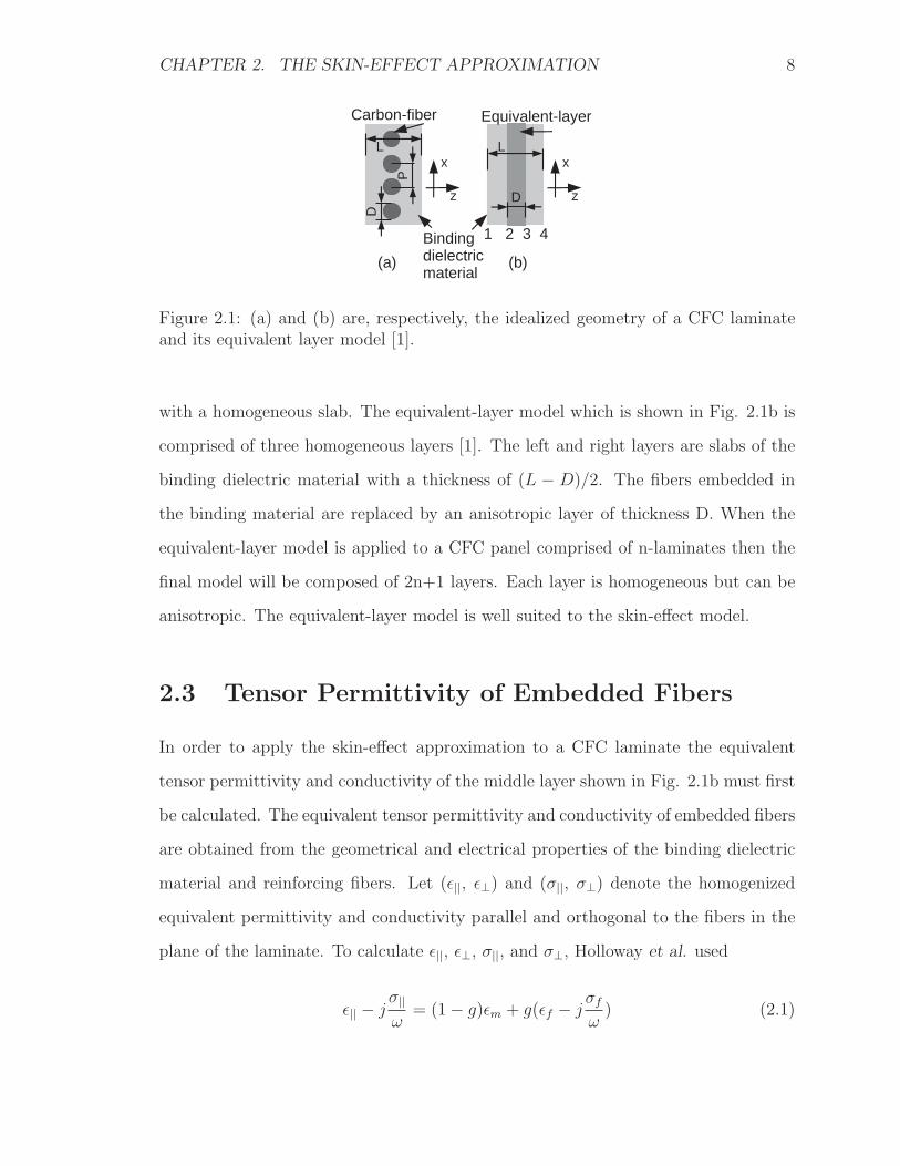
Figure 2.1: (a) and (b) are, respectively, the idealized geometry of a CFC laminateand its equivalent layer model [1].
with a homogeneous slab. The equivalent-layer model which is shown in Fig. 2.1b is
comprised of three homogeneous layers [1]. The left and right layers are slabs of the
binding dielectric material with a thickness of (L − D)/2. The fibers embedded in
the binding material are replaced by an anisotropic layer of thickness D. When the
equivalent-layer model is applied to a CFC panel comprised of n-laminates then the
final model will be composed of 2n+1 layers. Each layer is homogeneous but can be
anisotropic. The equivalent-layer model is well suited to the skin-effect model.
2.3 Tensor Permittivity of Embedded Fibers
In order to apply the skin-effect approximation to a CFC laminate the equivalent
tensor permittivity and conductivity of the middle layer shown in Fig. 2.1b must first
be calculated. The equivalent tensor permittivity and conductivity of embedded fibers
are obtained from the geometrical and electrical properties of the binding dielectric
material and reinforcing fibers. Let (ε||, ε⊥) and (σ||, σ⊥) denote the homogenized
equivalent permittivity and conductivity parallel and orthogonal to the fibers in the
plane of the laminate. To calculate ε||, ε⊥, σ||, and σ⊥, Holloway et al. used
ε|| − jσ||
ω= (1 − g)εm + g(εf − j
σf
ω) (2.1)

CHAPTER 2. THE SKIN-EFFECT APPROXIMATION 9
and [ε⊥ − j
σ⊥
ω
]−1
= (1 − g)εm−1 + g(εf − j
σf
ω)−1
(2.2)
where εm and εf are, respectively, the permittivity of the binding material and carbon-
fibers. σf is the conductivity of the fibers and the conductivity of the binding dielectric
material is assumed to be zero. Moreover, g is called the “volume fraction” of carbon-
fibers and is given by [1]
g =πD
4P. (2.3)
Material properties in the direction normal to the CFC laminate are not required
when using the skin-effect approximation because the laminate will be shrunk to a
sheet with zero thickness. In fact, the VEP currents normal to the plane of a CFC
laminate are ignored in the skin-effect approximation.
Now two dielectric materials should be created in FEKO with (ε||, σ||) and (ε⊥,
σ⊥) corresponding to the material properties along and orthogonal to the fibers orien-
tation. In the next section application of the skin effect approximation to a dielectric
slab is explained.
2.4 The Skin-Effect Approximation
Although the homogenization technique discussed in Section 2.2 greatly facilitates
simulation of the CFC laminate shown in Fig. 2.1a it is possible to further simplify
the equivalent-layer model shown in Fig. 2.1b. The typical thickness of a CFC
laminate is in the order of L=0.13 mm [28, 29]. If the tangential electric field is
approximately the same through the laminate then it is not necessary to calculate
electric and magnetic surface currents on the four boundaries in Fig. 2.1b. Since
CFC materials are not magnetic it is possible to replace the equivalent-layer model
shown in Fig. 2.1b with electric surface currents on a sheet. In fact, in the skin-effect
approximation the VEP currents are converted to surface currents provided that the
panel thickness is thin with respect to the material wavelength i.e., |γL| < 0.2 where
CHAPTER 2. THE SKIN-EFFECT APPROXIMATION 10
γ is the propagation constant in the laminate and L is the panel thickness [30].
A surface which supports an electric surface current such that Etan = ZsJs is
called an “impedance sheet” and Zs is referred to as the “sheet impedance”. For a
thin dielectric slab with a thickness of L, conductivity of σ and permittivity of ε the
equivalent sheet impedance is given by [31, 32]
Zs =β
2(σ + jωε − jωεe) sin(βL
2)
(2.4)
where β = ω√
μ0(ε + σ/jω) is the propagation constant in the dielectric material and
εe is the permittivity of the background medium. For lossless media σ = 0, ε and εe
are real and Zs will also be real. However, for lossy media σ �= 0 and β and Zs are
complex quantities. For an array of carbon-fibers embedded in a binding dielectric
material, Eqs. 2.1 and 2.2 are used to calculate the equivalent sheet impedance along
the laminate’s principal directions.
For the equivalent-layer model shown in Fig. 2.1b, FEKO recognizes three sheet
impedances corresponding to the three dielectric layers. In the next section, the three
impedance sheets will be merged into one sheet.
2.5 Stack-to-Sheet Conversion
There is usually more than one laminate in a CFC panel and the orientation of
the reinforcing fibers varies through the panel. Let ¯ZLsi represent the tensor sheet
impedance of the i-th laminate of a CFC panel with N laminates. Furthermore,
let Zsdi represent the sheet impedance of the left and right dielectric layers in the
equivalent-layer model of the i-th laminate. Finally, let Zs||i and Zs⊥i denote the
sheet impedance of the middle layer in the equivalent-layer model of the i-th laminate.
CHAPTER 2. THE SKIN-EFFECT APPROXIMATION 11
Then, ¯ZLsi is written as:
¯ZL
si =
⎧⎪⎨⎪⎩
⎡⎣ Zsdi 0
0 Zsdi
⎤⎦
−1
+
⎡⎣ Zs||i 0
0 Zs⊥i
⎤⎦−1
+
⎡⎣ Zsdi 0
0 Zsdi
⎤⎦−1
⎫⎪⎬⎪⎭
−1
. (2.5)
¯ZLsi is defined in a local coordinate system associated with the i-th laminate. In order
to describe the tensor sheet impedance of the i-th laminate in the panel’s coordinate
system the following transformation is used
¯ZP
si = ¯Ti¯Z
L
si¯Ti
−1(2.6)
where
¯T i =
⎡⎣ cos αi − sin αi
sin αi cos αi
⎤⎦ (2.7)
and αi is the angle that the fibers in the i-th laminate make with the panel’s reference
direction [32]. Finally, the tensor sheet impedance of a CFC panel with N laminates
in the panel’s coordinate system can be written as [31]:
¯Zs =
[N∑
i=1
¯ZPsi
−1
]−1
. (2.8)
The expression of ¯Zs is very similar to the overall impedance of multiple shunt loads
because it is assumed that the electric field is almost the same through the panel’s
thickness. In the skin-effect approximation, ¯Zs is used to calculate the surface currents
that penetrate CFC panels. The surface currents on a CFC panel are found such that
they reproduce the scattered fields of the original CFC panel. Using the skin-effect
approximation the fields everywhere in space are the summation of the incident and
scattered fields.
In the following section, the skin-effect model is used to calculate the reflection and
transmission coefficients of infinite CFC panels. Moreover, the magnetic SE inside a
hollow cubic shell with a CFC face is also obtained.
CHAPTER 2. THE SKIN-EFFECT APPROXIMATION 12
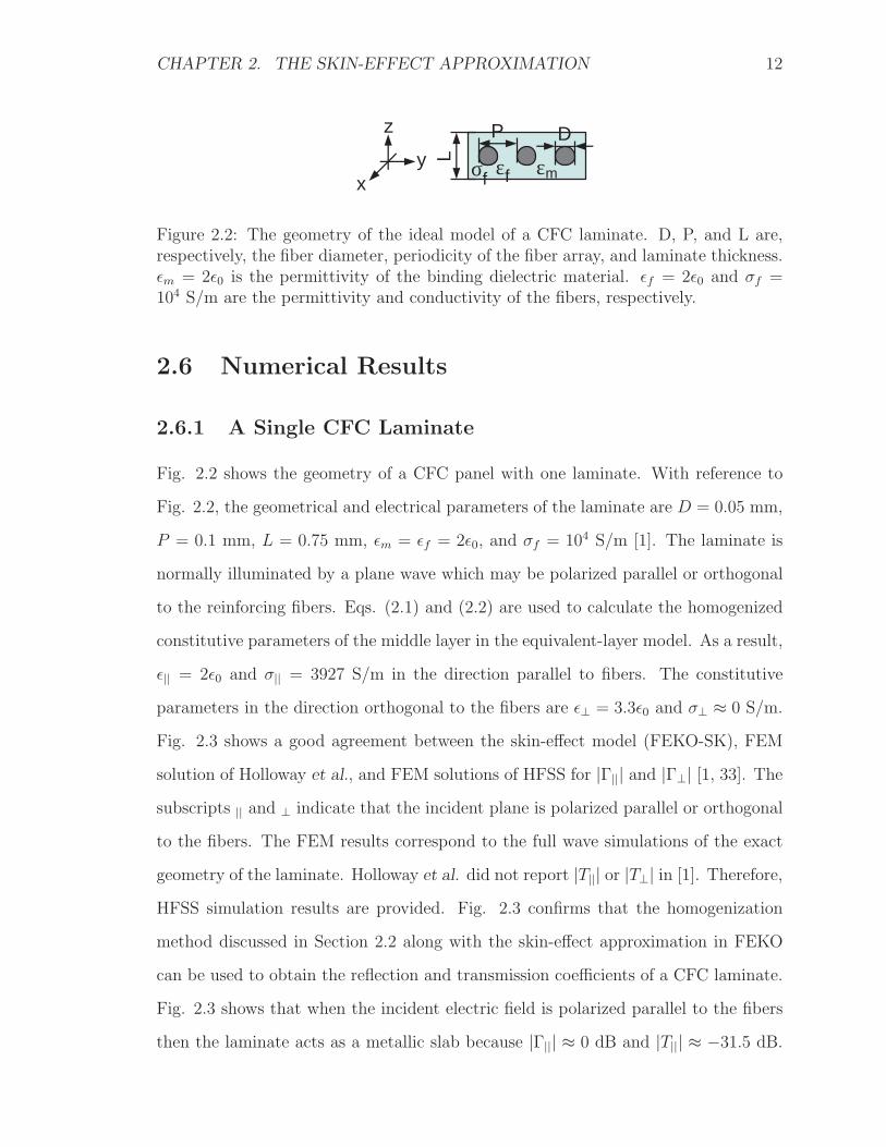
Figure 2.2: The geometry of the ideal model of a CFC laminate. D, P, and L are,respectively, the fiber diameter, periodicity of the fiber array, and laminate thickness.εm = 2ε0 is the permittivity of the binding dielectric material. εf = 2ε0 and σf =104 S/m are the permittivity and conductivity of the fibers, respectively.
2.6 Numerical Results
2.6.1 A Single CFC Laminate
Fig. 2.2 shows the geometry of a CFC panel with one laminate. With reference to
Fig. 2.2, the geometrical and electrical parameters of the laminate are D = 0.05 mm,
P = 0.1 mm, L = 0.75 mm, εm = εf = 2ε0, and σf = 104 S/m [1]. The laminate is
normally illuminated by a plane wave which may be polarized parallel or orthogonal
to the reinforcing fibers. Eqs. (2.1) and (2.2) are used to calculate the homogenized
constitutive parameters of the middle layer in the equivalent-layer model. As a result,
ε|| = 2ε0 and σ|| = 3927 S/m in the direction parallel to fibers. The constitutive
parameters in the direction orthogonal to the fibers are ε⊥ = 3.3ε0 and σ⊥ ≈ 0 S/m.
Fig. 2.3 shows a good agreement between the skin-effect model (FEKO-SK), FEM
solution of Holloway et al., and FEM solutions of HFSS for |Γ||| and |Γ⊥| [1, 33]. The
subscripts || and ⊥ indicate that the incident plane is polarized parallel or orthogonal
to the fibers. The FEM results correspond to the full wave simulations of the exact
geometry of the laminate. Holloway et al. did not report |T||| or |T⊥| in [1]. Therefore,
HFSS simulation results are provided. Fig. 2.3 confirms that the homogenization
method discussed in Section 2.2 along with the skin-effect approximation in FEKO
can be used to obtain the reflection and transmission coefficients of a CFC laminate.
Fig. 2.3 shows that when the incident electric field is polarized parallel to the fibers
then the laminate acts as a metallic slab because |Γ||| ≈ 0 dB and |T||| ≈ −31.5 dB.
CHAPTER 2. THE SKIN-EFFECT APPROXIMATION 13
-4
-3
-2
-1
0
1
2
3
4
0.01 0.1 1 10
|Γ|||
[dB
]
Frequency [GHz]
FEKO-SKFEM-Holloway
FEM-Exact Geometry-HFSS
-80
-70
-60
-50
-40
-30
-20
-10
0
0.01 0.1 1 10
|Γ⊥| [
dB]
Frequency [GHz]
FEKO-SKFEM-Holloway
FEM-Exact Geometry-HFSS
-40
-35
-30
-25
-20
-15
-10
-5
0
0.01 0.1 1 10
|T|||
[dB
]
Frequency [GHz]
FEKO-SKFEM-Exact Geometry-HFSS
-4
-3
-2
-1
0
1
0.01 0.1 1 10|T
⊥| [
dB]
Frequency [GHz]
FEKO-SKFEM-Exact Geometry-HFSS
Figure 2.3: The reflection and transmission coefficients of the CFC laminate shownin Fig. 2.2. A comparison is made between the skin-effect model and FEM solutionsreported by Holloway or obtained using HFSS. The subscripts || and ⊥ indicate thatthe incident plane wave is polarized parallel or orthogonal to the fibers.
However, if the incident electric field is polarized orthogonal to the fibers then the
laminate acts as a thin dielectric slab because |T⊥| ≈ 0 dB. In the following section,
the skin-effect model is applied to a CFC panel with two laminates.
2.6.2 CFC Panel with Two Laminates
Fig. 2.4 shows the geometry of an infinite CFC panel comprised of two laminates.
The geometrical structure and electrical properties of each laminate are the same as
those given in Section 2.6.1. The reinforcing fibers in the two laminates are oriented
orthogonal to one another. The panel is illuminated by Ei|| = yejk0z or Ei
⊥ = xejk0z
where k0 is the wavenumber of the incident plane wave in free space. The subscripts
|| and ⊥ indicate that the incident plane wave is polarized parallel or orthogonal to

CHAPTER 2. THE SKIN-EFFECT APPROXIMATION 14
Figure 2.4: The geometry of a CFC panel with two laminates. The reinforcing fibersare oriented along the y- and x-axis. The geometrical and electrical parameters ofeach laminate are given in Section 2.6.1.
-0.7-0.65-0.6
-0.55-0.5
-0.45-0.4
-0.35-0.3
-0.25-0.2
0.01 0.1 1 10 100
|Γ|||
[dB
]
Frequency [GHz]
FEKO-SKFEM-Exact Geometry-HFSS
-0.7-0.65-0.6
-0.55-0.5
-0.45-0.4
-0.35-0.3
-0.25-0.2
0.01 0.1 1 10 100
|Γ⊥| [
dB]
Frequency [GHz]
FEKO-SKFEM-Exact Geometry-HFSS
-34
-33
-32
-31
-30
-29
-28
0.01 0.1 1 10 100
|T|||
[dB
]
Frequency [GHz]
FEKO-SKFEM-Exact Geometry-HFSS
-34
-33
-32
-31
-30
-29
-28
0.01 0.1 1 10 100
|T⊥| [
dB]
Frequency [GHz]
FEKO-SKFEM-Exact Geometry-HFSS
FEM-Holloway
Figure 2.5: The reflection and transmission coefficients of a CFC panel with twolaminates for a normally incident plane wave. The panel is illuminated by a normallyincident plane wave polarized along the x- and y-axis.
the fibers oriented along the y-axis. Using the homogenization method discussed in
Section 2.2, the equivalent-layer model of each laminate is obtained and fed to the
skin-effect model in FEKO. Then, the reflection and transmission coefficients of the
panel are obtained using double periodic boundary conditions and simulation results
are shown in Fig. 2.5. The MoM solutions of the skin-effect model (FEKO-SK) are
compared with FEM solutions reported by Holloway et al. or obtained using HFSS
simulations [1]. The FEM solutions correspond to the full wave analysis of the unit cell
of the panel shown in Fig. 2.4. Holloway’s solutions were available only for |T⊥| [1].
CHAPTER 2. THE SKIN-EFFECT APPROXIMATION 15
Hence, HFSS simulation results are also presented. Fig. 2.5 shows that having fibers
oriented in two orthogonal orientations eliminated the strong anisotropic behavior of
a single CFC laminate. The magnitude of the reflection coefficients |Γ||| or |Γ⊥| is
almost 0 dB indicating that the incident plane wave is reflected and not absorbed
by the panel. Moreover, for f ≤ 10 GHz the tangential electric field is almost the
same through the panel’s thickness and |T||| ≈ |T⊥| ≈ −31.5 dB. In Section 2.6.1,
|T||| ≈ −31.5 dB for a single laminate. It is evident that the laminate in which
fibers are oriented orthogonal to the polarization of the incident plane wave does
not contribute in the SE. It is worth noting that since |Γ||| and |Γ⊥| are almost 0
dB they are not sensitive to the approximations that are made in the skin effect
model. However, Fig. 2.5 reveals that the skin-effect model has limitations in SE
calculations because the FEKO-SK solution for |T||| and |T⊥| start to deviate from
the exact solutions for f > 10 GHz.
For a homogeneous conducting panel the SE is due to reflection and absorption
[4]. The FEKO skin-effect model is capable of modeling only the reflection portion of
the shielding mechanism because the skin-effect approximation neglects the variations
of the electric field as the wave travels through the lossy material. Absorption loss
is about 1 dB when the material is one skin-depth thick. This is also the point at
which the skin-effect approximation begins to deteriorate. Therefore, as the panel’s
physical thickness increases the highest frequency at which the skin-effect model can
be used in SE calculations decreases. FEKO does not yet have the capability of using
the ABCD parameters of each laminate of a CFC panel to eliminate such limitations
on the panel’s thickness. To further elaborate this point, a CFC panel with four
laminates is simulated in the next section.
2.6.3 CFC Panel with Four Laminates
Fig. 2.6 shows the geometry of a CFC panel composed of four laminates. The reinforc-
ing fibers are oriented as 0/90/0/90 degrees with respect to the y-axis. The laminates
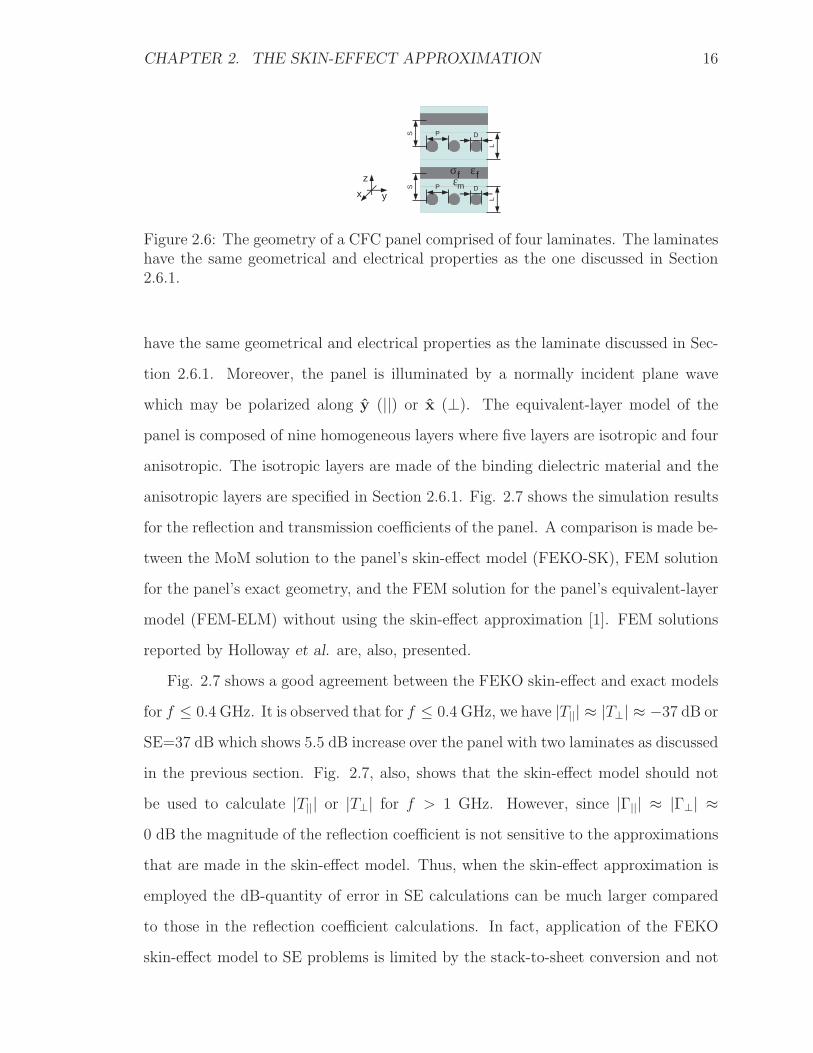
CHAPTER 2. THE SKIN-EFFECT APPROXIMATION 16
Figure 2.6: The geometry of a CFC panel comprised of four laminates. The laminateshave the same geometrical and electrical properties as the one discussed in Section2.6.1.
have the same geometrical and electrical properties as the laminate discussed in Sec-
tion 2.6.1. Moreover, the panel is illuminated by a normally incident plane wave
which may be polarized along y (||) or x (⊥). The equivalent-layer model of the
panel is composed of nine homogeneous layers where five layers are isotropic and four
anisotropic. The isotropic layers are made of the binding dielectric material and the
anisotropic layers are specified in Section 2.6.1. Fig. 2.7 shows the simulation results
for the reflection and transmission coefficients of the panel. A comparison is made be-
tween the MoM solution to the panel’s skin-effect model (FEKO-SK), FEM solution
for the panel’s exact geometry, and the FEM solution for the panel’s equivalent-layer
model (FEM-ELM) without using the skin-effect approximation [1]. FEM solutions
reported by Holloway et al. are, also, presented.
Fig. 2.7 shows a good agreement between the FEKO skin-effect and exact models
for f ≤ 0.4 GHz. It is observed that for f ≤ 0.4 GHz, we have |T||| ≈ |T⊥| ≈ −37 dB or
SE=37 dB which shows 5.5 dB increase over the panel with two laminates as discussed
in the previous section. Fig. 2.7, also, shows that the skin-effect model should not
be used to calculate |T||| or |T⊥| for f > 1 GHz. However, since |Γ||| ≈ |Γ⊥| ≈0 dB the magnitude of the reflection coefficient is not sensitive to the approximations
that are made in the skin-effect model. Thus, when the skin-effect approximation is
employed the dB-quantity of error in SE calculations can be much larger compared
to those in the reflection coefficient calculations. In fact, application of the FEKO
skin-effect model to SE problems is limited by the stack-to-sheet conversion and not

CHAPTER 2. THE SKIN-EFFECT APPROXIMATION 17
-0.7
-0.6
-0.5
-0.4
-0.3
-0.2
-0.1
0.01 0.1 1 10 100
|Γ|||
[dB
]
Frequency [GHz]
FEKO-SKFEM-Exact Geometry-HFSS
FEM-ELM-0.7
-0.6
-0.5
-0.4
-0.3
-0.2
-0.1
0.01 0.1 1 10 100
|Γ⊥| [
dB]
Frequency [GHz]
FEKO-SKFEM-Exact Geometry-HFSS
FEM-ELM
-75
-70
-65
-60
-55
-50
-45
-40
-35
0.01 0.1 1 10 100
|T|||
[dB
]
Frequency [GHz]
FEKO-SKFEM-Exact Geometry-HFSS
FEM-ELM-75
-70
-65
-60
-55
-50
-45
-40
-35
0.01 0.1 1 10 100|T
⊥| [
dB]
Frequency [GHz]
FEKO-SKFEM-Exact Geometry-HFSS
FEM-ELMFEM-Holloway
Figure 2.7: The reflection and transmission coefficients of a CFC panel with fourlaminates. The fibers in the panel are oriented as 0/90/0/90 degrees with respect tothe y-axis, as shown in Fig. 2.6. The panel is illuminated by a normally incidentplane wave which may be polarized along the y- (||) or x-axis (⊥).
the homogenization method discussed in Section 2.2. To prove this point, the FEM
solutions for the panel’s equivalent-layer model (FEM-ELM) are shown in Fig. 2.7.
The good agreement between the reflection and transmission coefficient of the exact
geometry and its equivalent-layer model proves that the stack-to-sheet conversion
limits application of the FEKO skin-effect model in SE calculations.
In the next section, the skin-effect model is applied to a finite structure.
2.6.4 Hollow Cubic Shell with a CFC Face
Fig. 2.8a shows a hollow cubic shell with a side length of W = 0.5 m. The front face
of the shell has a conductivity of σ = 4× 10⁴ S/m and thickness of d = 2 mm. Other
faces of the shell are copper with a conductivity of σCu = 5.7×10⁷ S/m and thickness

CHAPTER 2. THE SKIN-EFFECT APPROXIMATION 18
(a)
20 30 40 50 60 70 80 90
100 110 120 130
0.1 1 10 100
Mag
netic
SE
[dB
]
Frequency [MHz]
Kimmel-SingerFEKO-SK
Inside-outside
(b)
Figure 2.8: The magnetic SE at the center of a hollow cubic shell with a side length of0.5 m. All faces of the cube are copper with a thickness of 0.1 mm except for the frontface which is CFC with a thickness of 2 mm and conductivity of σ = 4 × 10⁴ S/m.A comparison is made between the skin-effect model, inside-outside formulation, andresults reported by Kimmel and Singer [2].
of 0.1 mm. The CFC face is illuminated by the plane wave Ei = 120πzejk0x V/m
where k0 = 2π/λ0 and λ0 is the wavelength of the incident plane wave in free space.
The electric and magnetic symmetries of the problem with respect to the z = 0 and
y = 0 planes are applied in order to accelerate the simulations. In this section, the
magnetic SE at the center of the cube is obtained using two different formulations, the
skin-effect model and inside-outside formulation. The inside-outside formulation is
the standard approach in FEKO for SE calculations as will be described in Chapter 5.
In the skin-effect approximation the simulation results for the SE are sensitive to the
discretization errors in the surface currents because inside conducting enclosures the
fields produced by the surface currents should almost perfectly cancel the incident
fields. In this section, the mesh size is progressively reduced until the simulation
results approached a final solution. The inside-outside formulation did not show such
dependence on the mesh size. The simulations results for the magnetic SE at the
center of the cube i.e., SE = |H(0, 0, 0)|no cube/|H(0, 0, 0)|cube are shown in Fig. 2.8b.
The FEKO simulations are performed for a mesh size of W/10. The shell is meshed
into 946 triangle surface elements. Furthermore, the total number of unknowns are,

CHAPTER 2. THE SKIN-EFFECT APPROXIMATION 19
respectively, 709 and 1418 in the skin-effect model and inside-outside formulation.
Fig. 2.8b shows very good agreement between the simulation results for the skin-
effect approximation and inside-outside formulation for f ≤ 1 MHz. Because σCu �σCFC the leakage through the copper faces can be ignored compared to the leakage
through the CFC face. At f = 1 MHz, the thickness of the CFC face is d = 0.8δs
and that is where the results of the skin-effect approximation start to deviate from
the other solutions as the frequency increases. An excellent agreement is observed
between the inside-outside formulation and published results [2]. The thickness of
the front face is d = 8δs at f = 100 MHz. If the dB-quantity of the SE is small and
is basically determined by the presence of apertures, cracks, or seams on the CFC
structure and not the leakage through a CFC skin then the skin-effect model might
be an efficient tool.
2.7 Conclusions
Using homogenization techniques and the FEKO skin effect model (“SK-card”) the
reflection and transmission coefficients of CFC panels were obtained and validated.
In the skin-effect model, an equivalent tensor sheet impedance was found such that
the total electric VEP currents that penetrate a CFC panel are reproduced on an
impedance sheet. The skin-effect model used stack-to-sheet conversion approach to
shrink CFC panels to an impedance sheet with zero thickness. As a result, the
scattered fields produced by CFC panels composed of a single or multiple laminates
could be calculated with no more simulation resources than what would be required
if the panel was PEC. This is the greatest merit of the skin-effect model especially
useful for electrically large structures, such as CFC aircraft. The tensor complex
permittivity of each laminate was calculated with homogenization techniques and
then used in the skin-effect model. For CFC panels with one, two, and four laminates
the FEKO MoM simulation results were compared and validated with published FEM

CHAPTER 2. THE SKIN-EFFECT APPROXIMATION 20
solutions or those of the HFSS. It was observed that the reflection coefficient of CFC
panels was not prone to errors associated with the skin-effect approximation because
often |Γ| ≈ 0 dB for CFC panels. The limitation of the skin-effect model in calculating
the SE of CFC panels with multiple laminates was shown to be caused by the stack-
to-sheet conversion and not homogenization techniques. Moreover, it was observed
that the fibers that were oriented orthogonal to the polarization of the incident plane
wave did not contribute in the shielding mechanism.
The plane wave magnetic SE at the center of a hollow cubic shell with a CFC
face was also calculated using the skin-effect model and the results were compared
with published literature and agreement was obtained for d ≤ 0.8δs. Although the
skin-effect model could be used in SE calculations a very fine mesh might have to
be used to eliminate discretization errors associated with the representation of the
surface currents in terms of the basis functions. This limitation can be overcome with
the inside-outside formulation. The skin-effect model is best used for calculating the
scattered fields of CFC structures. Moreover, if the SE is determined by apertures,
crack, and seams on a CFC structure and not leakage through a CFC material then
the skin-effect model might also be useful.
Chapter 3
Monopole Antennas on CFC
Structures
3.1 Introduction
A typical aircraft can use as many as 20 antennas for communication, navigation,
instrument landing systems, radar altimeter, and other purposes [34]. Therefore, in
this chapter, the reflection coefficient and radiation pattern of monopole antennas
mounted on metallic and CFC ground planes are experimentally examined [35].
The impact of replacing metals with CFC materials on the EMI inside CFC en-
closures is examined in this chapter. The electrical conductivity of a barrier plays a
key role in reducing the level of fields that leak into an enclosure and meeting EMC
requirements. The conductivity of CFC materials is 1000 times lower than that of
most metals [1]. Moreover, the permeability of CFC materials is basically that of the
free space. Therefore, the attenuation of EM waves propagating in CFC materials is
much lower compared to metals.
The term SE usually refers to the SE to electric fields [4]. The SE to magnetic
fields is more dependent on the barrier’s conductivity compared to the SE to electric
fields. Therefore in this chapter, the leakage of magnetic fields as well as electric fields
21

CHAPTER 3. MONOPOLE ANTENNAS ON CFC STRUCTURES 22
Figure 3.1: Monopole antennas mounted on metallic (top view) and CFC (top andbottom views) ground planes.
into enclosures are examined [4].
The skin depth is 1/√
πfμ0σ and approximately 32 times larger in CFC materials
compared to metals. Therefore, the difference between metallic and CFC shields
manifest at frequencies for which the metallic barrier is much thicker than the skin
depth in the barrier while a CFC replacement with the same physical thickness is not.
The CFC materials that are considered in this chapter have a thickness in the order
of 1 mm. For frequencies in the VHF and HF frequency bands the material thickness
is in the order of the skin depth. That is why in this chapter, the CFC shells are
simulated in the VHF and HF frequency bands.
This chapter is organized as follows. Section 3.2 presents the measurement results
for the reflection coefficient and radiation pattern of monopole antennas mounted on
metallic and CFC ground planes. Moreover, different methods of attaching an SMA
connector feed to a CFC ground plane are tested. In Sections 3.3 and 3.4, monopole
antennas are mounted on hollow aluminum or CFC cubic shells and operated at
the frequencies of 100 MHz and 3 MHz, respectively. FEKO simulation results for
the leaked electric and magnetic fields inside the shells are presented and discussed.
Finally, conclusions are made in Section 3.5.
3.2 Monopole Antennas on CFC Ground Planes
Two monopole antennas using CFC and metallic ground planes were built as shown
in Fig. 3.1. The ground planes are square with a side length of 15.24 cm. The
CHAPTER 3. MONOPOLE ANTENNAS ON CFC STRUCTURES 23
-30
-25
-20
-15
-10
-5
0
2 2.5 3 3.5 4 4.5 5
|S11
| [dB
]
Frequency [GHz]
STEELCFC
-30
-25
-20
-15
-10
-5
0
4 4.5 5 5.5 6 6.5 7 7.5 8
|S11
| [dB
]
Frequency [GHz]
STEELCFC
-30
-25
-20
-15
-10
-5
0
6 7 8 9 10 11 12
|S11
| [dB
]
Frequency [GHz]
STEELCFC
-30
-25
-20
-15
-10
-5
0
8 9 10 11 12 13 14 15 16|S
11| [
dB]
Frequency [GHz]
STEELCFC
Figure 3.2: A comparison between the measured reflection coefficient of monopoleantennas with CFC and steel ground planes operated at the frequencies of 3 GHz, 6GHz, 9 GHz, and 12.5 GHz.
material of the metallic ground plane is steel with a conductivity of 5.76 × 10⁶ S/m
[4, 36]. The CFC panel is reinforced with two layers of carbon-fiber fabrics. The fiber
bundles in the panel are oriented as 0/90/0/90 degrees [37]. The thickness of the CFC
ground plane is 0.635 mm. The diameter of the monopole wire is 0.61 mm. During
the measurement of the reflection coefficient, the lengths of the monopole antennas
were adjusted for the best return loss at the frequencies of 3 GHz, 6 GHz, 9 GHz,
and 12.5 GHz. The experiments are performed in order to examine effects of the
metallic feed-CFC panel connection on the antenna performance. Figs. 3.2 and 3.3
compare the measured reflection coefficient and radiation pattern of the monopole
antennas with CFC and steel ground planes. If we assume that the monopole wire
is on the z-axis and the ground plane is on the x-y plane then the radiation pattern
measurements are conducted such that the radiated Eθ in the plane of φ = 90◦ is

CHAPTER 3. MONOPOLE ANTENNAS ON CFC STRUCTURES 24
-40 -30 -20 -10 0
STEELCFC
(a)
-30 -20 -10 0
STEELCFC
(b)
-20 -10 0
STEELCFC
(c)
-20 -10 0
STEELCFC
(d)
Figure 3.3: (a)-(d) are a comparison between the normalized measured radiationpattern (|Gθ|) of monopole antennas with CFC and steel ground planes operated atthe frequencies of 3 GHz, 6 GHz, 9 GHz, and 12.5 GHz, respectively.
measured. The radiation pattern measurements were performed at the frequencies of
3 GHz, 6 GHz, 9 GHz, and 12.5 GHz and all patterns are normalized using the same
factor. It is observed that by replacing a metallic ground plane with a CFC panel the
return loss and radiation pattern of the antennas are practically unchanged even at
12.5 GHz.
The establishment of the electrical contact between the SMA connector and the
CFC panel is made by the two different methods which are shown in Figs. 3.4a and
3.4b. In the first method, the CFC sheet is sandpapered around the feed area so that
the carbon-fibers in the panel are exposed. Then, the area is cleaned and a conduc-
tive tape is attached to the feed area. Next, the SMA connector is soldered to the
conductive tape. In the second method, another copy of the same CFC panel is used.

CHAPTER 3. MONOPOLE ANTENNAS ON CFC STRUCTURES 25
(a) (b)
Figure 3.4: Two methods of attaching an SMA connector to a CFC panel, (a) withand (b) without a patch of conducting tape.
However, no conductive tapes are employed and the feed area is not sandpapered.
The SMA connector is simply attached to the CFC panel using two bolts and nuts
as shown in Fig. 3.4b. The monopole antennas were operated at 3 GHz, 6 GHz,
9 GHz, and 12.5 GHz. The measured reflection coefficient of the antennas did not
show dependence on the feed attachment method. In other words, both techniques
provided enough coupling between the panel and SMA connector. It is believed that
current flow from the SMA connector to the CFC panel can be established either
through the conduction currents between the conductive tape and the carbon-fibers
in the panel or through displacement currents through the capacitance that is formed
by mounting the SMA feed on the CFC panel.
3.3 Interference Due to VHF Antennas
Fig. 3.5 shows a monopole antenna mounted on a hollow cubic shell. The cubic
shell has a side length of W = 3 m and thickness of t = 1 mm representing part
of an aircraft fuselage. Two materials for the shell are considered aluminum σAl =
3.96×10⁷ S/m [36] and CFC σ = 104 S/m. The monopole wire is PEC with a diameter
of D = 6 mm and length of l = 75 cm. The monopole antenna is fed at the intersection
of the monopole wire and top face of the shell using a “vertex port” in FEKO. In this
section, the monopole antenna is operated at the VHF frequency of f = 100 MHz and
delivered an active power of 1 W. At f = 100 MHz, the shell thickness equals to 2δs
and 125δs in CFC and aluminum, respectively. The MoM solver is used to calculate

CHAPTER 3. MONOPOLE ANTENNAS ON CFC STRUCTURES 26
Figure 3.5: A monopole antenna mounted on a hollow cubic shell with a side lengthof W = 3 m and thickness of t = 1 mm. The monopole wire is PEC with a length ofl = 75 cm and diameter of D = 6 mm. The material of the shell can be aluminum orCFC.
surface currents inside and outside of the shell and line currents on the wire. The
magnetic symmetries with respect to the x-z, and y-z planes are imposed in order
to accelerate the simulations. The monopole wire is modeled using the thin wire
assumption because D = 0.002λ0 λ0. Since fields inside the hollow shell are much
weaker compared to fields outside the shell the surface currents inside and outside the
shell are designated as unknowns by filling the shell with a dielectric material with
a relative permittivity of unity [5]. The wire and the shell are meshed into 7 wire
segments and 4912 triangle surface elements using the fine mesh settings in FEKO.
The total number of unknowns is 3617. The electric and magnetic fields on the y-z
plane inside the hollow shell are obtained and shown in Fig. 3.6. Figs. 3.6a and 3.6b
reveal that there is practically no leakage of EM fields from outside into inside the
aluminum shell. At the frequency of 100 MHz the thickness of the aluminum slab is
t = 1 mm= 125δs where δs is the skin depth in aluminum. In fact, the magnitude of
the leaked electric and magnetic fields are in the order of 10−57 V/m and 10−60 A/m.
Furthermore, Figs. 3.6a and 3.6b could be made only on a linear scale because the
fields were so weak.
CHAPTER 3. MONOPOLE ANTENNAS ON CFC STRUCTURES 27
(a) Aluminum (b) Aluminum
(c) CFC (d) CFC
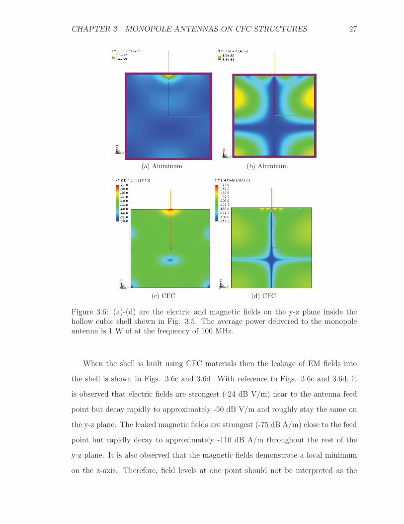
Figure 3.6: (a)-(d) are the electric and magnetic fields on the y-z plane inside thehollow cubic shell shown in Fig. 3.5. The average power delivered to the monopoleantenna is 1 W of at the frequency of 100 MHz.
When the shell is built using CFC materials then the leakage of EM fields into
the shell is shown in Figs. 3.6c and 3.6d. With reference to Figs. 3.6c and 3.6d, it
is observed that electric fields are strongest (-24 dB V/m) near to the antenna feed
point but decay rapidly to approximately -50 dB V/m and roughly stay the same on
the y-z plane. The leaked magnetic fields are strongest (-75 dB A/m) close to the feed
point but rapidly decay to approximately -110 dB A/m throughout the rest of the
y-z plane. It is also observed that the magnetic fields demonstrate a local minimum
on the z-axis. Therefore, field levels at one point should not be interpreted as the

CHAPTER 3. MONOPOLE ANTENNAS ON CFC STRUCTURES 28
field level everywhere inside the shell.
3.4 Interference Due to HF Antennas
In this section, the monopole antenna shown in Fig. 3.5 is operated at the frequency
of 3 MHz. At f = 3 MHz, the shell thickness equals to 0.34δs and 22δs in CFC
and aluminum, respectively. 22δs is very thick, but 0.34δs of the CFC shell shows
potential for leakage. The geometry of the antenna is not modified and the mismatch
between the monopole antenna and a 50 Ω transmission line is not of concern because
FEKO is set up to automatically multiply all surface currents with an appropriate
factor such that an active power of 1 W is delivered to the antenna. As a result,
a comparison can be made between the leaked electric and magnetic fields into the
shell at HF and VHF frequencies. At f = 3 MHz, we have λ0 = 100 m. The side
length of the shell is W = 3 m= 0.03λ0 which is considered to be electrically small.
Therefore, the mesh size is chosen based on the variations of the surface currents
from one edge to other edges and not based on the wavelength. The simulations are
repeated with progressively smaller mesh sizes until variations of the simulated leaked
fields to the mesh size are negligible. A mesh size of W/18 = λ0/600 is found to be
small enough to represent surface currents on the shell because by choosing smaller
mesh sizes the magnitude of the leaked electric and magnetic fields close to the feed
point vary by a value smaller than 3 dB. The monopole wire and shell are meshed into
5 wire segments and 6232 triangle surface elements. The total number of unknowns
is 4597. Figs. 3.7a and 3.7b show the magnitude of the leaked electric and magnetic
fields on the y-z plane inside the aluminum shell. It is observed that the strongest
electric and magnetic fields inside the shell are in the order of -210 dB V/m and -225
dB A/m near to the feed point. Figs. 3.7c and 3.7d show the magnitude of the leaked
electric and magnetic fields on the y-z plane if aluminum is replaced with CFC in
constructing the shell. It is observed that the strongest leaked electric and magnetic

CHAPTER 3. MONOPOLE ANTENNAS ON CFC STRUCTURES 29
(a) Aluminum (b) Aluminum
(c) CFC (d) CFC
Figure 3.7: The electric and magnetic fields on the y-z plane inside the hollow cubicshell shown in Fig. 3.5. The average power delivered to the monopole is delivered 1W of at the frequency of 3 MHz.
fields inside the CFC shell are in the order of 7.5 dB V/m and -7.5 dB A/m near to
the feed point. Furthermore, electric and magnetic fields decay rapidly away from the
feed point. Fig. 3.7 shows that by replacing metals with CFC materials variations of
the electric and magnetic fields are approximately preserved but the fields strength
are increased.

CHAPTER 3. MONOPOLE ANTENNAS ON CFC STRUCTURES 30
3.5 Conclusions
This chapter showed that by replacing a metallic ground plane with a CFC one the
measured radiation pattern and feed point reflection coefficient of monopole anten-
nas remained practically unchanged for frequencies up to 12.5 GHz. Moreover, no
conductive tapes or sandpapering the feed area was found to be necessary to operate
the monopole antennas on CFC ground planes. Although the antenna performance
did not change by replacing a metallic ground plane with a CFC one the EMI inside
CFC enclosures was much larger compared to an equivalent metallic enclosure.
Monopole antennas were mounted on hollow aluminum and CFC cubic shells and
operated in the VHF and HF frequency bands. FEKO simulation results showed
that by changing the enclosure’s material from aluminum to CFC the field patterns
inside the shell did not change but the magnitude of the leaked electric and magnetic
fields were increased. In fact, the contrast between CFC and metallic shields of the
same physical thickness was a source of concern at frequencies for which the barriers
thickness is much larger compared to the skin depth in the metallic material but not
in the CFC. It was observed that the maximum leakage of EM fields inside the shell
occurred in the vicinity of the antenna feed point and could be 70 dB larger compared
to other locations away from the feed area. The leakage into the shell was increased
as the frequency decreased. Moreover, the quantity of the fields at one point should
not be interpreted as the quantity of the fields everywhere in the shell because of the
possibility of the occurrence of local nulls in the field’s pattern inside the shell. When
the side length of the cubic shell was much smaller than the free space wavelength
the mesh size was chosen based on the variations of the surface currents on the shell
and not merely based on the wavelength.
Chapter 4
Effects of Interlaminar Bondings
4.1 Introduction
The model of CFC materials which is used by Holloway et al. does not take into ac-
count the bonding between the reinforcing fibers in adjacent laminates [1]. However,
other authors have shown that bonding between orthogonally oriented wires changes
the reflection and transmission coefficients of wire meshes in free space. According to
Hill and Wait, unbonded wire meshes have “superior reflecting properties” compared
to the bonded wire meshes [17, 24, 25, 26]. Therefore, in this chapter the effects of
bonding between the reinforcing fibers on the transmission and reflection coefficient
of CFC materials are investigated. The CFC panel used in Chapter 3 was reinforced
with woven fabrics. In other words, the reinforcing carbon-fibers were packed in
ribbon-shaped bundles and then woven before the final CFC panel is produced. In
this thesis, such a woven bundle of carbon-fibers is called a carbon-fiber fabric. The
effects of bonding between orthogonally oriented carbon-fiber bundles on the reflec-
tion and transmission coefficient of CFC panels are also investigated. The electrical
contact at the junction of bonded reinforcements is assumed to be ideal i.e., zero con-
tact resistance. In this chapter, effects of embedding wire meshes with bonded and
unbonded junctions in a dielectric slab on the reflection and transmission coefficients
31
CHAPTER 4. EFFECTS OF INTERLAMINAR BONDINGS 32
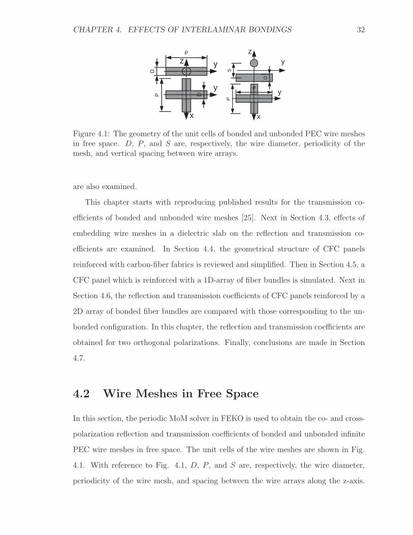
Figure 4.1: The geometry of the unit cells of bonded and unbonded PEC wire meshesin free space. D, P , and S are, respectively, the wire diameter, periodicity of themesh, and vertical spacing between wire arrays.
are also examined.
This chapter starts with reproducing published results for the transmission co-
efficients of bonded and unbonded wire meshes [25]. Next in Section 4.3, effects of
embedding wire meshes in a dielectric slab on the reflection and transmission co-
efficients are examined. In Section 4.4, the geometrical structure of CFC panels
reinforced with carbon-fiber fabrics is reviewed and simplified. Then in Section 4.5, a
CFC panel which is reinforced with a 1D-array of fiber bundles is simulated. Next in
Section 4.6, the reflection and transmission coefficients of CFC panels reinforced by a
2D array of bonded fiber bundles are compared with those corresponding to the un-
bonded configuration. In this chapter, the reflection and transmission coefficients are
obtained for two orthogonal polarizations. Finally, conclusions are made in Section
4.7.
4.2 Wire Meshes in Free Space
In this section, the periodic MoM solver in FEKO is used to obtain the co- and cross-
polarization reflection and transmission coefficients of bonded and unbonded infinite
PEC wire meshes in free space. The unit cells of the wire meshes are shown in Fig.
4.1. With reference to Fig. 4.1, D, P , and S are, respectively, the wire diameter,
periodicity of the wire mesh, and spacing between the wire arrays along the z-axis.

CHAPTER 4. EFFECTS OF INTERLAMINAR BONDINGS 33
0 0.1 0.2 0.3 0.4 0.5 0.6 0.7 0.8 0.9
1
0 5 10 15 20 25 30 35 40 45
|Γ..|
ϕ°
P=0.25λ0D=0.04Pθ=70°Bonded
|Γθθ||Γϕϕ||Γϕθ||Γθϕ|
0 0.1 0.2 0.3 0.4 0.5 0.6 0.7 0.8 0.9
1
0 5 10 15 20 25 30 35 40 45
|Γ..|
ϕ°
P=0.25λ0D=0.04Pθ=70°S=1.5DUnbonded
|Γθθ||Γϕϕ||Γϕθ||Γθϕ|
0 0.1 0.2 0.3 0.4 0.5 0.6 0.7 0.8 0.9
1
0 5 10 15 20 25 30 35 40 45
|T..|
ϕ°
P=0.25λ0D=0.04Pθ=70°Bonded
|Tθθ|Hill-Wait |Tθθ|
|Tϕϕ|Hill-Wait |Tϕϕ|
|Tϕθ||Tθϕ|
0 0.1 0.2 0.3 0.4 0.5 0.6 0.7 0.8 0.9
1
0 5 10 15 20 25 30 35 40 45
|T..|
ϕ°
P=0.25λ0D=0.04PS=1.5Dθ=70°
Unbonded
|Tθθ|Hill-Wait |Tθθ|
|Tϕϕ|Hill-Wait |Tϕϕ|
|Tθϕ|Hill-Wait |Tθϕ|
|Tϕθ|Hill-Wait |Tϕθ|
Figure 4.2: A comparison between FEKO simulation and results of Hill and Wait [3]for the co-polarization and cross-polarization transmission coefficients of bonded andunbonded PEC thin wire meshes in free space versus the azimuth angle φ.
The wire meshes have square unit cells because the periodicity is the same along
the x- and y-axis. The wire meshes are illuminated by an incident plane wave at an
oblique incident angle of θ = 70◦. The elevation angle θ is measured with respect
to the z-axis and θ = 0 denotes normal incidence. This incidence angle was chosen
by Hill and Wait and the behavior of the wire meshes at other incidence angles of
θ are not examined here [3]. The incident plane wave may be polarized along φ
or θ in the spherical coordinate system. The θ-polarization (φ-polarization) is such
that the incident plane wave is parallel (perpendicular) to the plane of incidence. The
frequency of the incident plane wave is such that P = λ0/4 where λ0 is the wavelength
of the incident plane wave in free space. By optionally choosing f = 1 GHz as the
simulation frequency, the parameters in Fig. 4.1 become D = 3 mm, P = 75 mm,
and S = 4.5 mm. The wires are analyzed using the thin wire assumption because

CHAPTER 4. EFFECTS OF INTERLAMINAR BONDINGS 34
0
0.2
0.4
0.6
0.8
1
1.2
0 10 20 30 40 50 60 70 80 90
|Γ..|
ϕ°
P=0.01λ0
D=0.04Pθ=70°S=0Bonded
|Γϕϕ||Γθϕ||Γθθ||Γϕθ|
0 0.1 0.2 0.3 0.4 0.5 0.6 0.7 0.8 0.9
1 1.1
0 10 20 30 40 50 60 70 80 90
|Γ..|
ϕ°
P=0.01λ0
D=0.04Pθ=70°S=1.5DUnbonded
|Γϕϕ||Γθϕ||Γθθ||Γϕθ|
0
0.01
0.02
0.03
0.04
0.05
0.06
0.07
0.08
0 10 20 30 40 50 60 70 80 90
|T..|
ϕ°
P=0.01λ0D=0.04Pθ=70°S=0Bonded
|Tϕϕ||Tθϕ||Tθθ||Tϕθ|
0
0.01
0.02
0.03
0.04
0.05
0.06
0.07
0.08
0 10 20 30 40 50 60 70 80 90
|T..|
ϕ°
P=0.01λ0D=0.04Pθ=70°S=1.5DUnbonded
|Tϕϕ||Tθϕ||Tθθ||Tϕθ|
Figure 4.3: The co- and cross-polarization reflection and transmission coefficients ofbonded and unbonded wire meshes in free space (Fig. 4.1) versus the azimuth angleφ for an oblique incident plane wave with θ = 70◦ at a frequency where P = λ0/100.
D λ0. The geometries shown in Fig. 4.1 are simulated and results are presented
in Fig. 4.2. With reference to Fig. 4.2, |Γφθ| denotes the magnitude of the reflection
coefficient for the φ polarized reflected plane wave due to a θ-polarized incident plane
wave.
Hill and Wait employed a MoM solution using the Fourier expansion of the induced
currents on the wires to calculate the reflection and transmission coefficients of the
wire meshes. In the case of the bonded wire mesh, a discontinuity in the wire currents
at the junction was also applied [17, 24, 25, 26]. Fig. 4.2 shows a good agreement
between the results reported by Hill and Wait [25] and those produced by FEKO. The
following conclusions are made from Fig. 4.2: 1) Bonded wire meshes may be assumed
isotropic even when P = λ0/4 because the transmission and reflection transmission
coefficients are, almost, independent of the azimuth angle φ and the cross-polarization

CHAPTER 4. EFFECTS OF INTERLAMINAR BONDINGS 35
components are negligible compared to the co-polarization components [25]. 2) The
co-polarization transmission coefficient of an unbonded wire mesh is generally smaller
than that of the bonded [17].
The reflection and transmission coefficients of bonded and unbonded wire meshes
shown in Fig. 4.1 are simulated again when the frequency of the incident plane wave
is reduced to f = 40 MHz (P = λ0/100) while the wire mesh is not changed. The
results are shown in Fig. 4.3. It is observed that the co- and cross-polarization trans-
mission and reflection coefficients of the unbonded wire mesh for θ- or φ-polarized
incident plane waves still show azimuth dependence despite P λ0. Moreover, for the
unbonded mesh, the cross-polarization components in the transmitted and reflected
waves are not negligible compared to the respective co-polarization components.
In summary, unbonded wire meshes in free space generally have a lower trans-
mission coefficient compared to the bonded. However, unbonded wire meshes have
an azimuth-dependent transmission coefficient and produce cross-polarization com-
ponents.
4.3 Wire Meshes Embedded in Epoxy
The wire meshes that were discussed in the previous section are embedded in an
infinite dielectric slab as shown in Fig. 4.4. The slab has a thickness of L = 4D =
12 mm where D is the wire diameter. The material of the dielectric slab is “epoxy
resin” or simply epoxy which is widely used in manufacturing CFC materials for the
aerospace industry [7]. The permittivity of epoxy resin is εm = 3.6ε0 [4]. The purpose
of this section is to examine effects of embedding bonded and unbonded wire meshes
in an epoxy slab. With reference to Fig. 4.4, the co- and cross-polarization reflection
and transmission coefficients of the embedded wire meshes are obtained for an oblique
incident plane wave. The incident plane wave propagates inward and makes an angle
of θ = 70◦ with the z-axis. The incident plane wave can be polarized along θ or φ in

CHAPTER 4. EFFECTS OF INTERLAMINAR BONDINGS 36
Figure 4.4: The geometry of the bonded and unbonded wire meshes embedded inan infinite dielectric epoxy slab. The thickness of the dielectric slab is L = 4D. D,P , and S are, respectively, the wire diameter, periodicity of the mesh, and verticalspacing between wire arrays. The wires are assumed to be PEC and the permittivityof the dielectric slab is epoxy with εm = 3.6ε0 [4].
the spherical coordinate system. If the incident plane wave is polarized along φ then
the incident electric field is parallel to the slab. The simulations are performed at
f = 40 MHz and f = 1 GHz which correspond to P = 0.01λ0 and P = 0.25λ0 and λ0
is the wavelength of the incident plane wave in vacuum. Therefore, the reflection and
transmission properties may be identified in a wide frequency range. The embedded
wire meshes shown in Fig. 4.4 are simulated using FEKO and the results are given
in Fig. 4.5. With reference to Figs. 4.5(a)-4.5(d), the following conclusions at P =
0.01λ0 are made: 1) The co-polarization reflection and transmission coefficients have
variations of less than 1 dB when the azimuth angle of the incident plane wave varies
from 0◦ to 90◦. Moreover, the cross polarization components in the transmitted waves
are more than 10 dB lower compared to the co-polarization components. Therefore,
the embedded bonded and unbonded wire meshes may be considered isotropic. 2)
For the embedded bonded and unbonded wire meshes, the transmission coefficient is
approximately 17 dB larger for a θ-polarized incident plane wave compared to a φ-
polarized one. 3) Embedding wire meshes in epoxy reduces effects of bonding between
orthogonally oriented wires because the co-polarization transmission coefficients of
the embedded unbonded wire mesh is less than 1 dB smaller than that of the bonded

CHAPTER 4. EFFECTS OF INTERLAMINAR BONDINGS 37
0 0.1 0.2 0.3 0.4 0.5 0.6 0.7 0.8 0.9
1
0 10 20 30 40 50 60 70 80 90
|Γ..|
ϕ°
BondedP=0.01λ0D=0.04P
θ=70°L=4D
|Γϕϕ||Γθϕ||Γθθ||Γϕθ|
(a)
0
0.2
0.4
0.6
0.8
1
0 10 20 30 40 50 60 70 80 90
|Γ..|
ϕ°
UnbondedP=0.01λ0D=0.04P
S=1.5Dθ=70°L=4D
|Γϕϕ||Γθϕ||Γθθ||Γϕθ|
(b)
0
0.02
0.04
0.06
0.08
0.1
0.12
0.14
0.16
0 10 20 30 40 50 60 70 80 90
|T..|
ϕ°
Bonded
P=0.01λ0
D=0.04P
θ=70°
L=4D|Tϕϕ||Tθϕ||Tθθ||Tϕθ|
(c)
0
0.02
0.04
0.06
0.08
0.1
0.12
0.14
0.16
0 10 20 30 40 50 60 70 80 90|T
..|ϕ°
Unbonded
P=0.01λ0
D=0.04P
S=1.5D
θ=70°
L=4D |Tϕϕ||Tθϕ||Tθθ||Tϕθ|
(d)
0
0.2
0.4
0.6
0.8
1
0 10 20 30 40 50 60 70 80 90
|Γ..|
ϕ°
BondedP=0.25λ0D=0.04P
θ=70°L=4D
|Γϕϕ||Γθϕ||Γθθ||Γϕθ|
(e)
0
0.2
0.4
0.6
0.8
1
0 10 20 30 40 50 60 70 80 90
|Γ..|
ϕ°
UnbondedP=0.25λ0D=0.04P
S=1.5Dθ=70°L=4D
|Γϕϕ||Γθϕ||Γθθ||Γϕθ|
(f)
0
0.2
0.4
0.6
0.8
1
0 10 20 30 40 50 60 70 80 90
|T..|
ϕ°
BondedP=0.25λ0D=0.04P
θ=70°L=4D
|Tϕϕ||Tθϕ||Tθθ||Tϕθ|
(g)
0
0.2
0.4
0.6
0.8
1
0 10 20 30 40 50 60 70 80 90
|T..|
ϕ°
UnbondedP=0.25λ0D=0.04P
S=1.5Dθ=70°L=4D
|Tϕϕ||Tθϕ||Tθθ||Tϕθ|
(h)
Figure 4.5: (a)-(h) are the co- and cross-polarization reflection and transmissioncoefficients of bonded and unbonded wire meshes embedded in an infinite epoxy slabversus the azimuth angle φ at an oblique incidence angle of θ = 70◦. Two frequenciesare chosen such that P = 0.01λ0 and P = 0.25λ0.

CHAPTER 4. EFFECTS OF INTERLAMINAR BONDINGS 38
Figure 4.6: The surface of a CFC panel reinforced with two sets of carbon-fiber fabricsoriented as (0/90)/(0/90) degrees. The fabrics have a plain weave structure.
configuration.
Next, the frequency of the incident plane wave is increased to f = 1 GHz where
P = 0.25λ0; the simulation results are shown in Figs. 4.5(e)-4.5(h). The level of
cross-polarization components and azimuth-angle dependence of the reflection and
transmission coefficients are slightly increased. Moreover, it is observed that em-
bedding bonded and unbonded wire meshes in an epoxy slab reduces the difference
between the two structures. The transmission coefficient of the embedded unbonded
structure is approximately 1 dB lower than that of the bonded.
In summary, embedding wire meshes in an epoxy slab made the bonding between
the orthogonally oriented wires less important.
4.4 Woven Reinforcements
The surface of a CFC panel with woven reinforcements is shown in Fig. 4.6 [37].
This is the same panel that was used in Chapter 3 as antenna ground plane. The
panel is composed of two layers of carbon-fiber fabrics embedded in an epoxy host

CHAPTER 4. EFFECTS OF INTERLAMINAR BONDINGS 39
Figure 4.7: (a)-(c) are, respectively, the unit cells of a 1D, 2D-bonded, and 2D-unbonded arrays of carbon-fiber fabrics embedded in a dielectric slab. Moreover,P = 2.2 mm, W = 2 mm, t = 0.159 mm, and g = 0.0159 mm. The dielectric slabhas a permittivity of εm = 3.6ε0 and the carbon-fiber bundles have a conductivity ofσ = 104 S/m.
medium [37]. The panel has a thickness of L = 0.635 mm. The exact geometry of
a woven structure is available in [38]. For simplicity, the entanglement associated
with the weaves is ignored and the cross section of the bundles is approximated to be
rectangular with a width of W = 2 mm and thickness of t = L/4 = 0.159 mm. The
permittivity and conductivity of the fiber bundles are assumed to be ε0 and 104 S/m,
respectively. The epoxy slab is lossless with a permittivity of εm = 3.6ε0 [4]. Although
the panel shown in Fig. 4.6 is reinforced with two layers of carbon-fiber fabrics the
panels simulated in this chapter are reinforced with reinforcements shown in Fig. 4.7.
Moreover, it is assumed that the CFC panel is infinite so that plane wave reflection
and transmission coefficients may be defined. Based on the geometry shown in Fig.
4.6, the periodicity of the panel is assumed to be P = 2.2 mm along the x- and y-axis.
Based on the physical structure of the panel, the three geometries shown in Fig. 4.7
are conceived. The panel with a 1D array of reinforcements serves as a reference panel.
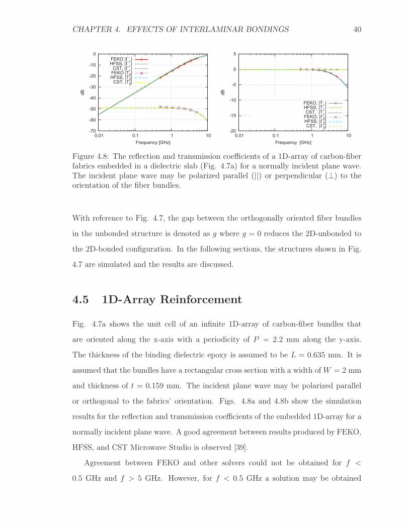
CHAPTER 4. EFFECTS OF INTERLAMINAR BONDINGS 40
-70
-60
-50
-40
-30
-20
-10
0
0.01 0.1 1 10
dB
Frequency [GHz]
FEKO |Γ⊥|HFSS, |Γ⊥|
CST, |Γ⊥|FEKO |T|||HFSS, |T|||
CST, |T|||
-20
-15
-10
-5
0
5
0.01 0.1 1 10
dB
Frequency [GHz]
FEKO, |T⊥|HFSS, |T⊥|CST, |T⊥|
FEKO, |Γ|||HFSS, |Γ|||CST, |Γ|||
Figure 4.8: The reflection and transmission coefficients of a 1D-array of carbon-fiberfabrics embedded in a dielectric slab (Fig. 4.7a) for a normally incident plane wave.The incident plane wave may be polarized parallel (||) or perpendicular (⊥) to theorientation of the fiber bundles.
With reference to Fig. 4.7, the gap between the orthogonally oriented fiber bundles
in the unbonded structure is denoted as g where g = 0 reduces the 2D-unbonded to
the 2D-bonded configuration. In the following sections, the structures shown in Fig.
4.7 are simulated and the results are discussed.
4.5 1D-Array Reinforcement
Fig. 4.7a shows the unit cell of an infinite 1D-array of carbon-fiber bundles that
are oriented along the x-axis with a periodicity of P = 2.2 mm along the y-axis.
The thickness of the binding dielectric epoxy is assumed to be L = 0.635 mm. It is
assumed that the bundles have a rectangular cross section with a width of W = 2 mm
and thickness of t = 0.159 mm. The incident plane wave may be polarized parallel
or orthogonal to the fabrics’ orientation. Figs. 4.8a and 4.8b show the simulation
results for the reflection and transmission coefficients of the embedded 1D-array for a
normally incident plane wave. A good agreement between results produced by FEKO,
HFSS, and CST Microwave Studio is observed [39].
Agreement between FEKO and other solvers could not be obtained for f <
0.5 GHz and f > 5 GHz. However, for f < 0.5 GHz a solution may be obtained

CHAPTER 4. EFFECTS OF INTERLAMINAR BONDINGS 41
by using a larger unit cell. In the non-periodic solver metallic media in FEKO could
be used for t ≤ δs or t ≥ δs where t is the material thickness and δs is the skin-
depth. However, in the periodic solver the carbon-fiber bundles had to be modeled
as lossy dielectric materials because t ≥ δs. But using a lossy dielectric instead of
metallic medium introduces a new problem of λ λ0 while meshing and simulating
the geometry for f > 5 GHz.
Figs. 4.8a and 4.8b show that at frequencies below 1 GHz, if the incident plane
wave is polarized orthogonal to the bundles then the embedded 1D-array acts as a
lossless dielectric slab. However, if the incident plane wave is polarized parallel to
the bundles then the embedded 1D-array behaves as a lossy conducting slab. Fur-
thermore, the transmission coefficient of the embedded 1D-array for a normally inci-
dent plane wave polarized parallel to the fibers orientation is |T||| = −49 dB. Since
|Γ||| ≈ 0 dB for f ≤ 1 GHz the incident plane wave is reflected and not absorbed by
the panel.
4.6 2D-Bonded and Unbonded Reinforcements
Figs. 4.7b and 4.7c show the geometries of the 2D-bonded and 2D-unbonded arrays
of fiber bundles that are embedded in an epoxy slab. The gap between the orthog-
onally oriented fiber bundles is denoted as g. In order to examine bonding effects
the gap should be chosen small compared to the bundles thickness t; Therefore, g is
chosen as t/10. Fig. 4.9 shows the reflection and transmission coefficients of the CFC
panels with 2D-bonded and 2D-unbonded reinforcements for two normally incident
plane waves polarized along x or y. The simulations are performed using FEKO,
HFSS, and CST Microwave Studio and a good agreement between the solutions are
obtained. Figs. 4.9a-4.9d show that at normal incidence, the transmission and re-
flection coefficient of the 2D-bonded structure is not dependent on the polarization
of the incident plane wave for f ≤ 1 GHz. Moreover, the transmission coefficient of

CHAPTER 4. EFFECTS OF INTERLAMINAR BONDINGS 42
-0.5
-0.4
-0.3
-0.2
-0.1
0
0.01 0.1 1 10
|Γ..|
[dB
]
Frequency [GHz]
Bonded
||-||, HFSS||-||, CST||-||, FEKO⊥-⊥, HFSS⊥-⊥, CST⊥-⊥, FEKO
(a)
-0.5
-0.4
-0.3
-0.2
-0.1
0
0.01 0.1 1 10
|Γ..|
[dB
]
Frequency [GHz]
Unbonded
||-||, HFSS||-||, CST
||-||, FEKO⊥-⊥, HFSS
⊥-⊥, CST⊥-⊥, FEKO
(b)
-120
-110
-100
-90
-80
-70
-60
-50
-40
0.01 0.1 1 10
|T..|
[dB
]
Frequency [GHz]
Bonded
||-||, HFSS||-||, CST||-||, FEKO⊥-⊥, HFSS⊥-⊥, CST⊥-⊥, FEKO
(c)
-120
-110
-100
-90
-80
-70
-60
-50
-40
0.01 0.1 1 10
|T..|
[dB
]
Frequency [GHz]
Unbonded
||-||, HFSS||-||, CST
||-||, FEKO⊥-⊥, HFSS
⊥-⊥, CST⊥-⊥, FEKO
(d)
Figure 4.9: The reflection and transmission coefficients of the 2D-bonded and 2D-unbonded carbon-fiber bundles embedded in a dielectric slab, as shown in Figs. 4.7band 4.7c. The incident plane wave propagates normal to the panels and can bepolarized along the x-axis (||) or y-axis (⊥). ||-|| (⊥-⊥) represents the co-polarizationcomponent of the reflection or transmission coefficient when the incident plane waveis polarized along the x-axis (y-axis).
the 2D-unbonded configuration is -49 dB for f ≤ 1 GHz which equals to that of the
1D-array discussed in the previous section. Fig. 4.9c shows that the transmission
coefficient of the bonded structure is -54 dB for f ≤ 1 GHz.
In summary, bonding orthogonally oriented carbon-fiber bundles causes the fiber
bundles that are oriented orthogonal to the polarization of the incident plane wave
to attenuate the incident plane wave also. This is an important conclusion which
may be used in increasing the SE of CFC materials. At f = 1 GHz, the bundles
thickness equals to the skin depth in the carbon-fibers. For f ≤ 1 GHz, the bundles
are completely penetrated by the incident plane wave and the SE is provided by

CHAPTER 4. EFFECTS OF INTERLAMINAR BONDINGS 43
reflection. For f > 1 GHz, absorption of the incident plane wave in the carbon-fibers
also contributes in SE. That is why the transmission coefficients start to decrease for
f > 1 GHz.
4.7 Conclusions
In this chapter, effects of the bonding between orthogonally oriented wires or fiber
bundles were investigated. It was assumed that structures under consideration are
infinite panels so that the double periodic boundary conditions could be employed
in the simulations. The wires were assumed to be PEC and were modeled using the
thin wire approximation. For wire meshes in free space, FEKO simulation results for
the co- and cross-polarization transmission coefficients were validated with published
results. It was observed that unbonded wire meshes in free space were preferable
over the bonded wire meshes from a SE point of view. However, embedding the
wire meshes in an epoxy slab reduced the effects of bonding on the transmission and
reflection coefficients. In other words, although unbonded wire meshes in free space
are preferable over bonded wire meshes from a SE point of view, that advantage is
weakened by embedding unbonded wire meshes in a dielectric material. The reflection
and transmission coefficients of CFC panels with reinforcements in the form of fiber
bundles were obtained. It was assumed that the reinforcing fiber bundles had a
rectangular cross section with a width of 2 mm and thickness of 0.159 mm. The
fiber bundles were modeled using lossy dielectric materials with a conductivity of
104 S/m. Simulation results showed that bonded fiber bundles were preferable over
the unbonded from a SE point of view. In fact, the bondings caused the bundles
that are oriented orthogonal to the polarization of the incident plane to contribute in
the shielding process. This is a useful point which may be employed to enhance the
shielding capabilities of CFC panels.

Chapter 5
Shielding Effectiveness of CFC
Enclosures
5.1 Introduction
CFC materials can be modeled as isotropic lossy conducting media with a conductivity
in the order of σ = 104 S/m [15]. In this chapter, the capabilities and limitations of
FEKO in modeling conducting materials are investigated. The focus is on the Surface
Integral Equations (SIE) solutions to SE problems involving CFC materials. By
default, FEKO treats conducting materials as impedance sheets rather than generally
penetrable objects because fields decay very rapidly inside conducting materials [32].
FEKO User’s manual recommends Modeling conducting materials using “Metallic
Media” [32]. “Metallic Media” that are bound by free space regions are modeled
as impedance sheets [32]. The sheet impedance Zs is the proportionality constant
between the tangential electric field and the electric surface currents on the sheet
[32]. The value of the sheet impedance is automatically calculated by FEKO. If
the sheet impedance has been obtained through measurement techniques or other
analytical solutions then the user can also use custom values for the sheet impedance.
In order to validate FEKO’s ability in calculating large SE quantities inside CFC
44

CHAPTER 5. SHIELDING EFFECTIVENESS OF CFC ENCLOSURES 45
(a) (b)
Figure 5.1: (a) and (b) are the FEKO Simulation results for the total electric fieldinside a hollow spherical PEC shell with a radius of 3 m for an incident plane wavegiven by E = ze−jk0y at the frequency of 100 MHz. In case (a) fields inside the shellare obtained using the free space MoM whereas in case (b) fields are obtained byusing the inside-outside formulation [5].
enclosures certain benchmark solutions are generated in this chapter.
This chapter is outlined as follows. In Section 5.2, the inside-outside formulation is
elaborated and its difference with the free space MoM is explained. An infinite CFC
panel modeled as a lossy dielectric material is simulated in FEKO and the results
are compared with the analytic solution in Section 5.3. In Section 5.4, benchmark
numerical results for the electric and magnetic SE inside a hollow spherical CFC shell
are presented and compared with FEKO simulation results. Finally, conclusions are
made in Section 5.5.
5.2 The Inside-Outside SIE Formulation
If a closed PEC surface is bound by free space regions then FEKO uses the free
space MoM to find the electric surface currents on the PEC surface such that the
scattered and incident electric fields cancel each other everywhere inside the PEC
shell. This requires perfect cancellation of the tangential components of the incident
and scattered electric fields everywhere on the PEC surface. In fact, a very small

CHAPTER 5. SHIELDING EFFECTIVENESS OF CFC ENCLOSURES 46
error in the cancellation of the tangential electric fields causes large SE errors on the
dB-scale [5].
Fig. 5.1a shows the cross sectional view of a hollow spherical PEC shell with a
radius of 3 m which is illuminated by a plane wave with a frequency of 100 MHz. The
shell is bound by free space regions in the FEKO model and the free space MoM is
used to solve the problem by default. Using the standard mesh settings, the electric
fields inside the shell on the x-y plane are obtained and results are shown in Fig. 5.1a.
The magnitude of the electric fields inside the shell should be 0 V/m or −∞ dB V/m.
Effects of the imperfect cancellation of the incident and scattered fields are evident
in Fig. 5.1a. It is observed that the electric fields produced by the surface currents
on shell are capable of canceling the incident electric field down to a range of -22.5
dB V/m to -90 dB V/m. Fig. 5.1a also shows that the error tends to be larger in the
vicinity of the walls of the shell.
If the SIE is formulated such that total fields inside the shell are given by one
set of electric surface currents and the scattered fields outside the shell are obtained
by another set of surface currents then the inside-outside formulation is obtained [5].
Obviously, the inside-outside formulation is based on the surface equivalence principle
(SEP) [40]. Using the inside-outside formulation, perfect cancellation of the incident
and scattered fields inside the PEC shell is no longer required and large SE quantities
can be obtained. In order to replace the free space MoM with the inside-outside
formulation the only requirement is to change the material inside the hollow PEC
shell from free space to a dielectric material with a relative permittivity of unity
[5]. Having done that, the electric fields inside the shell are shown in Fig. 5.1b. It is
observed that the magnitude of the electric fields inside shell is now as low as -1000 dB
V/m. In fact, 0.0 on a linear scale is shown as -1000 dB on a dB-scale in FEKO. The
magnitude of the magnetic fields inside the shell is not shown for the sake of brevity
but they are also -1000 dB A/m on the x-y plane inside the shell. Application of
the inside-outside SIE formulation requires twice as many unknowns as the free space

CHAPTER 5. SHIELDING EFFECTIVENESS OF CFC ENCLOSURES 47
(a)
-70
-60
-50
-40
-30
-20
-10
0
1 10
|T| [
dB]
Frequency [GHz]
AnalyticTEL=2.5λ
TEL=λ
(b)
Figure 5.2: (a) The geometry of the unit cell of an infinite CFC panel modeled as adielectric material with σ = 104 S/m. The panel thickness is 0.159 mm. The triangleedge length (TEL) denotes the mesh size in FEKO. TEL is expressed in terms of thewavelength in the CFC panel. (b) The transmission coefficient of the panel shown inFig. 5.2a for a normally incident plane wave. The incident plane wave is polarizedalong the x-axis and its frequency varies from 1 GHz to 20 GHz.
MoM. In return, it makes it possible to calculate very large SE quantities. In Section
5.4, capabilities of the inside-outside formulation will be further explored. The SE of
the simplest closed CFC structure which is an infinite CFC slab is calculated in the
next section.
5.3 SE of an Infinite CFC Panel
In order to obtain the SE of an infinite CFC panel whose thickness is larger than
the skin-depth in the material a solution could only be obtained if the panel were
modeled as a lossy dielectric material with σ = 104 S/m. The geometry of the
problem is shown in Fig. 5.2. The panel has a thickness of t = 0.159 mm and the
double periodic boundary conditions are used in the simulations.
The transmission coefficient of the panel for a normally incident plane wave is
calculated in the frequency range of 1 GHz to 20 GHz. The skin depth in the panel is
δs = 0.159 mm and δs = 0.036 mm at f = 1 GHz and f = 20 GHz, respectively. The
width of the unit cell in Fig. 5.2 is chosen as W = 5λ where λ is the wavelength in

CHAPTER 5. SHIELDING EFFECTIVENESS OF CFC ENCLOSURES 48
the panel at the frequency of the incident plane wave. Inside the CFC panel and at
f = 1 GHz, λ = 1 mm but λ0 = 300 mm; consequently, we have W = 5λ = λ0/6 = 5
mm. Although in the FEKO examples guide a unit cell size of λ0/2 was employed a
choice of W = λ0/6 had to be made because the periodic solver crashed for W > λ0/6
[41].
The simulation results for the transmission coefficient of the panel are compared
with the analytic solution in Fig. 5.2b. The simulations are performed with two
different mesh sizes i.e., triangle edge length (TEL)=2.5λ and TEL=λ. Fig. 5.2b
shows that satisfactory results are obtained only for TEL=λ. It should be noted
that at normal incidence the surface currents are constant with no variations on the
surface. In other words, Fig. 5.2b shows that in SE calculations the mesh size on the
surface of a dielectric material should be chosen smaller than or equal to the material
wavelength.
The SIE formulation associated with Poggio, Miller, Chang, Harrington, Wu and
Tsai (PMCHWT) is used by FEKO to model dielectric materials. In other words,
FEKO uses the PMCHWT formulation to calculate the surface currents on the top
and bottom faces of the unit cell. In the PMCHWT formulation, the SEP is em-
ployed to postulate the existence of equivalent electric and magnetic surface currents
on the boundary of the scatterer such that Js and Ms produce the scattered fields
outside the scatterer but the total fields inside the obstacle. Js and Ms are found
by imposing boundary conditions associated with the continuity of the tangential
electric and magnetic fields on the boundary of the scatterer. The elements of the
MoM matrix in the PMCHWT formulation are dependent on the wavelength in the
conducting material as well as the free space wavelength [42, 43]. For materials with
a conductivity in the order of 104 S/m, this leads to an excessive simulation time and
loss of accuracy in SE problems. Therefore, instead of using the exact formulation
alternative SIE formulations along with approximate boundary conditions are widely
used when modeling conducting media.

CHAPTER 5. SHIELDING EFFECTIVENESS OF CFC ENCLOSURES 49
Therefore, modeling CFC panels as lossy dielectric materials in SE calculations
requires extensive simulation resources and is not efficient. In order to eliminate the
dependence of the mesh size to the material wavelength the inside-outside formulation
is employed in FEKO [5].
5.4 SE Inside a Hollow CFC Shell
In this section, it is assumed that a hollow spherical CFC shell in free space is illu-
minated by a plane wave of Ei = xe−jk0z where k0 = 2πf√
μ0ε0 and f varies in the
range of 1 MHz to 100 MHz. The shell has a radius of 3 m, thickness of 1 mm, and
conductivity of σ = 104 S/m. The shell’s center is coincident with the origin of the
coordinate system. In this section, we are interested in calculating the electric and
magnetic fields inside the shell.
The problem of scattering by concentric spheres is considered in [44]. Calculating
the analytic solution for the SE inside a hollow spherical shell is straightforward [45].
However, if the shell is a made of a conducting material with σ = 104 S/m then
the analytic solutions could not be numerically evaluated because of an overflow in
the involving Schelkunoff Bessel functions. A method is developed to eliminate this
problem and is presented in Appendix A.
The procedure for defining the problem in FEKO is as follows. At first, a metallic
medium named “cfc” with a conductivity of 104 S/m is defined. Next, a dielectric
medium named “air” with a relative permittivity of unity is created. Then, a solid
sphere with a radius of 3 m is constructed in FEKO and the material of the sphere
is changed from the default PEC to “air”. Finally, the surface (“face”) of the sphere
is set to be “cfc” with a thickness of 1 mm. Fig. 5.3 shows the FEKO simulation
results and the analytic solutions for the electric fields |E(x = 0, y = 0, z = 0)| and
normalized magnetic fields |η0H(x = 0, y = 0, z = 0)| at the shell’s center; η0 is the
characteristic impedance of the free space. The SE to electric or magnetic fields at
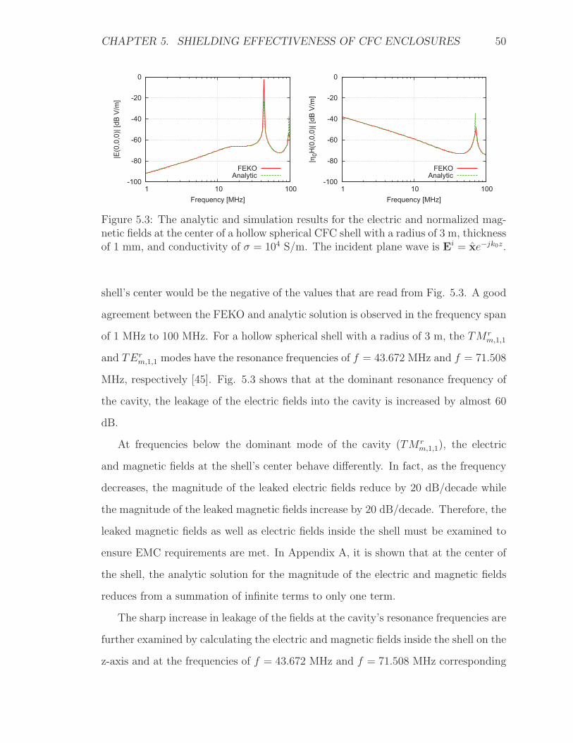
CHAPTER 5. SHIELDING EFFECTIVENESS OF CFC ENCLOSURES 50
-100
-80
-60
-40
-20
0
1 10 100
|E(0
,0,0
)| [d
B V
/m]
Frequency [MHz]
FEKOAnalytic
-100
-80
-60
-40
-20
0
1 10 100
|η0H
(0,0
,0)|
[dB
V/m
]
Frequency [MHz]
FEKOAnalytic
Figure 5.3: The analytic and simulation results for the electric and normalized mag-netic fields at the center of a hollow spherical CFC shell with a radius of 3 m, thicknessof 1 mm, and conductivity of σ = 104 S/m. The incident plane wave is Ei = xe−jk0z.
shell’s center would be the negative of the values that are read from Fig. 5.3. A good
agreement between the FEKO and analytic solution is observed in the frequency span
of 1 MHz to 100 MHz. For a hollow spherical shell with a radius of 3 m, the TM rm,1,1
and TErm,1,1 modes have the resonance frequencies of f = 43.672 MHz and f = 71.508
MHz, respectively [45]. Fig. 5.3 shows that at the dominant resonance frequency of
the cavity, the leakage of the electric fields into the cavity is increased by almost 60
dB.
At frequencies below the dominant mode of the cavity (TM rm,1,1), the electric
and magnetic fields at the shell’s center behave differently. In fact, as the frequency
decreases, the magnitude of the leaked electric fields reduce by 20 dB/decade while
the magnitude of the leaked magnetic fields increase by 20 dB/decade. Therefore, the
leaked magnetic fields as well as electric fields inside the shell must be examined to
ensure EMC requirements are met. In Appendix A, it is shown that at the center of
the shell, the analytic solution for the magnitude of the electric and magnetic fields
reduces from a summation of infinite terms to only one term.
The sharp increase in leakage of the fields at the cavity’s resonance frequencies are
further examined by calculating the electric and magnetic fields inside the shell on the
z-axis and at the frequencies of f = 43.672 MHz and f = 71.508 MHz corresponding

CHAPTER 5. SHIELDING EFFECTIVENESS OF CFC ENCLOSURES 51
-60
-50
-40
-30
-20
-10
0
-1 -0.8 -0.6 -0.4 -0.2 0 0.2 0.4 0.6 0.8 1
|E(0
,0,z
)| [d
B V
/m]
z/a
f= 43.672 MHz
FEKOAnalytic
-60
-50
-40
-30
-20
-10
0
-1 -0.8 -0.6 -0.4 -0.2 0 0.2 0.4 0.6 0.8 1
|η0H
(0,0
,z)|
[dB
V/m
]
z/a
f= 43.672 MHz
AnalyticFEKO
-60
-50
-40
-30
-20
-10
0
-1 -0.8 -0.6 -0.4 -0.2 0 0.2 0.4 0.6 0.8 1
|E(0
,0,z
)| [d
B V
/m]
z/a
f= 71.508 MHz
FEKOAnalytic
-60
-50
-40
-30
-20
-10
0
-1 -0.8 -0.6 -0.4 -0.2 0 0.2 0.4 0.6 0.8 1
|η0H
(0,0
,z)|
[dB
V/m
]
z/a
f= 71.508 MHz
AnalyticFEKO
Figure 5.4: The analytic and simulation results for the electric and magnetic fieldson the z-axis inside a hollow spherical CFC shell with a radius of 3 m, thickness of1 mm, and conductivity of σ = 104 S/m. The incident plane wave is Ei = xe−jk0z
where k0 is wavenumber of the incident plane wave at the frequencies of 43.672 MHzand 71.508 MHz.
to the TM rm,1,1 and TEr
m,1,1 resonances of the spherical cavity. Fig. 5.4 shows a very
good agreement between the FEKO simulation results and analytic solutions for the
electric and magnetic fields on the z-axis. In order to obtain the agreement, the mesh
size is chosen as TEL=λ0/20 where λ0 is the wavelength of the incident plane wave in
free space. The SE of an infinite CFC panel with a thickness of 1 mm to a normally
incident plane wave at f = 43.672 MHz is 66 dB. However, the electric SE of the
same CFC material when used as a hollow spherical shell can be as low as 15 dB at
cavity resonances. Fig. 5.4 shows that the magnetic SE inside the shell can be as low
as 10 dB at cavity resonances.
CHAPTER 5. SHIELDING EFFECTIVENESS OF CFC ENCLOSURES 52
5.5 Conclusions
This chapter was focused on the calculation of the electric and magnetic SE inside
CFC enclosures. It was observed that an approximate solution based on using metallic
media in FEKO should replace the exact PMCHWT formulation when modeling
penetrable materials with σ = 104 S/m. This was proved by showing that the if a
CFC panel is modeled as a lossy dielectric material then the mesh size has to be chosen
as small as the wavelength in the CFC material. Using the problem of scattering by a
hollow spherical PEC shell, the free space MoM and inside-outside formulations were
compared. In the free space MoM formulation the sum of the surface currents on the
inner and outer sides of the PEC shell was calculated and the fields everywhere in
space were the summation of the incident and scattered fields. Using this formulation
the maximum SE that could be calculated near to the walls of a shell was limited to
22.5 dB. This is because the cancellation of the incident and scattered fields could
not be perfect because of discretization of the surface currents and finite precision
arithmetic operations. It was shown that the inside-outside formulation is capable of
calculating SE quantities as large as 1000 dB at the expense of doubling the number
of unknowns. In the inside-outside formulation, the electric surface currents inside
and outside the shell were individually calculated. In order to replace the free space
MoM with the inside-outside formulation in FEKO the CFC panel should be backed
by a dielectric material with a permittivity of ε0.
For the SE inside a hollow spherical CFC shell, FEKO simulation results were
compared with the analytic solution and a good agreement was obtained. To calculate
SE quantities inside the shell the mesh size was chosen as λ0/20 which is smaller than
the default value of λ0/12. It was observed that the SE was significantly compromised
at the cavity’s resonance frequencies. At frequencies much smaller than the dominant
resonance of the cavity, as the frequency was decreasing, the electric SE increased by
20 dB/decade while the magnetic SE decreased by 20 dB/decade. While evaluating
the benchmark analytic solutions for the SE inside a hollow spherical CFC shell

CHAPTER 5. SHIELDING EFFECTIVENESS OF CFC ENCLOSURES 53
certain numerical difficulties were encountered and resolved.

Chapter 6
Conclusions and Future Work
6.1 Conclusions
A literature survey in Chapter 1 showed that CFC materials could be modeled as
conducting materials with a conductivity in the order of 104 S/m. Furthermore,
the radiation pattern and gain of antennas that were mounted on metallic ground
planes were practically unchanged by replacing the ground plane with a CFC one.
Therefore, the focus of the thesis was on the calculation of the SE of CFC structures
using FEKO.
In Chapter 2, the reflection and transmission coefficients of the idealized model
of CFC panels with one, two, and four laminates were obtained with the FEKO
skin-effect approximation and the results were validated with published literature
and other commercially available software. Using homogenization techniques the in-
homogeneous structure of the idealized model of CFC panels were simplified to an
equivalent multilayer structure. All layers of the equivalent multilayer model were
homogeneous but certain layers were anisotropic. The tensor conductivity and per-
mittivity of each layer of the equivalent multilayer model were specified in FEKO. A
stack-to-sheet conversion approach was used to shrink the equivalent multilayer model
to an impedance sheet with zero thickness. Using the skin-effect approximation the
54
CHAPTER 6. CONCLUSIONS AND FUTURE WORK 55
total VEP currents that penetrated a CFC panel were reproduced on an impedance
sheet. Furthermore, the VEP currents normal to a CFC panel were ignored. The ten-
sor sheet impedance of a CFC panel was found such that the tangential electric field
in the panel equaled to that on the impedance sheet. Therefore, the CFC panel had
to be thin with respect to the material wavelength so that the electric field was almost
constant in the panel. It was observed that approximations made in the skin-effect
model could be ignored in simulation results for the reflection coefficient. However,
simulation results for the transmission coefficient were in agreement with exact solu-
tions only if the panel was thin with respect to the material wavelength. It was shown
that the stack-to-sheet conversion and not the homogenization techniques limited the
largest frequency at which the FEKO skin-effect approximation could be used in SE
calculations. Furthermore, to use the skin-effect approximation the panel’s physical
thickness had to be thin compared to the panel’s lateral dimensions. The magnetic
SE at the center of a hollow cubic shell with a CFC face was calculated using the skin-
effect and inside-outside approaches and the results were compared with published
literature. Although results of the skin-effect model were in agreement with other
solutions when the panel’s thickness was smaller than or equal to the skin-depth,
application of the skin-effect approximation in SE calculations required a very fine
mesh. That said, for a fixed mesh size, the skin-effect model created as many un-
knowns as if the CFC panel composed of multiple laminates was simply a PEC sheet.
This was the greatest merit of the skin-effect approximation which made it useful for
calculating the far-zone scattered fields of electrically large CFC structures, such as
aircraft. In fact, if a CFC panel is not quasi-isotropic or its thickness is not larger
than the skin depth in the panel then it must be modeled as a laminated material
using the skin-effect approximation rather than a PEC sheet.
In Chapter 3, it was shown that the reflection coefficient and radiation pattern
of monopole antennas operated up to a frequency of 12.5 GHz were not altered if
the metallic ground plane was replaced by a much lighter CFC one. Sandpapering
CHAPTER 6. CONCLUSIONS AND FUTURE WORK 56
the feed area or using conductive tapes were found to be unnecessary for operating
monopole antennas mounted on CFC ground planes.
Monopole antennas mounted on metallic and CFC cubic shells were operated at
the frequency of 3 MHz and 100 MHz and the radiated EMI inside the shells were
calculated. It was shown that by replacing aluminum with CFC the pattern of the
leaked fields did not change but the strength of the leaked fields increased. It was
observed that as the frequency decreased effects of the lower conductivity of CFC
panels compared to the metallic ones became more of concern because a CFC barrier
with the same physical thickness as the metallic panel might no longer be much thicker
than the skin-depth in the barrier. The maximum leakage of EM fields inside a cubic
CFC enclosure occurred near to the feed point and could be 70 dB larger compared
to other locations in the shell away from the feed point. The leakage of EM fields into
the shell increased as the frequency decreased. Furthermore, the quantity of fields at
one point could not be interpreted as the general value of fields in CFC enclosures.
In Chapter 4, effects of bonding between orthogonally oriented reinforcements
were examined. PEC wire meshes were modeled using the thin wire assumption and
reinforcements in the form of carbon-fiber bundles had to be modeled as dielectric
materials with σ = 104 S/m. The published results for the co- and cross-polarization
transmission coefficients of bonded and unbonded wire meshes were reproduced using
the periodic MoM solver in FEKO. It was observed that in free space, wire meshes
with unbonded junctions were preferable to wire meshes with bonded junctions from
a SE standpoint. However, bonded wire meshes were more isotropic compared to
the unbonded and created weaker cross-polarization components. It was shown that
embedding wire meshes in an epoxy slab weakened effects of the bonding at the
junctions.
Based on the geometry of a purchased CFC panel, reinforcements in the form of
carbon-fiber bundles were conceived. The carbon-fiber bundles had a width of 2 mm
and thickness of 0.159 mm. It was shown that bonding the junctions improved the SE

CHAPTER 6. CONCLUSIONS AND FUTURE WORK 57
of CFC panels with reinforcements in the form of carbon-fiber bundles. Furthermore,
in the case of unbonded junctions the reinforcements that were oriented orthogonal
to the orientation of the polarization of the incident plane wave were transparent to
a normally incident plane wave. Moreover, the periodic solver in FEKO took much
longer simulation time compared to HFSS or CST Microwave Studio for the same
problem involving carbon-fiber bundles.
Chapter 5 was focused on EM modeling of conducting materials with σ = 104 S/m
in SE calculations. To calculate the SE of an infinite CFC panel at a frequency
for which the panel’s thickness was larger than the skin-depth the panel had to be
modeled as a dielectric material with σ = 104 S/m. It was observed that the exact
PMCHWT formulation which was used for modeling dielectric materials required
that the mesh size be determined by the wavelength in the CFC material and not
free space. Therefore, approximate instead of exact formulations were adapted for
calculating the SE of conducting structures.
The maximum dB-quantity of the SE that could be obtained using the free space
MoM was found to be very sensitive to the numerical errors associated with the
cancellation of the incident and scattered fields. Furthermore, the free space MoM
was based on calculating the sum of the surface currents on both sides of sheets while
the inside-outside formulation calculated currents on each side of sheets. That was the
reason that the inside-outside formulation created twice as many unknowns as the free
space MoM did. The total fields inside a hollow spherical PEC shell illuminated by a
plane wave were calculated using the free space MoM and inside-outside formulations.
When the free space MoM was employed, the electric fields inside the shell were in
the order of -22.5 dB V/m near to the walls of the shell while in the inside-outside
formulation the electric fields were in the order of -1000 dB V/m.
The SE quantities obtained using the inside-outside formulation were validated
by creating benchmark solutions for the SE inside a hollow spherical CFC shell. The
analytic solution needed to be modified to overcome the overflow of the Schelkunoff
CHAPTER 6. CONCLUSIONS AND FUTURE WORK 58
Bessel functions that were associated with the conducting media. In order to obtain
agreement with the benchmark solutions FEKO simulations were performed using
the inside-outside formulation and a mesh size of λ0/20 instead of the default value
of λ0/12. At frequencies below the resonance of the dominant mode of the spherical
cavity the SE to electric fields increased by 20 dB/decade as the frequency decreased
but the magnetic SE was decreasing with the same rate. The SE could be reduced
by 60 dB at the resonance frequencies of the spherical cavity.
6.2 Future Work
In future work, the periodic MoM solver in FEKO should be accelerated because at
this time the FEKO’s periodic solver often requires a much longer simulation time
compared to other commercially available FEM or finite integration technique (FIT)
solvers.
The CFC panel reinforced with carbon-fiber bundles was simulated up to 10 GHz.
It would be advantageous to simulate the panel at higher frequencies and verify the
simulation results and the differences between the bonded and unbonded configura-
tions. Moreover, effects of a non-zero contact resistance at the junctions of bonded
and unbonded reinforcements on the SE can also be investigated.
Materials with σ = 104 S/m cannot always be treated using the inside-outside
formulation e.g., a periodic array of carbon-fiber bundles. In fact, it is necessary to
modify the MoM solver so that it can efficiently handle materials with σ = 104 S/m
in SE calculations using an exact SIE formulation.
The inside-outside formulation in FEKO could not be applied to anisotropic lay-
ered media. This is another feature that can be added to FEKO.
It would be interesting to examine the reduction of the electric and magnetic SE of
non-spherical hollow CFC shells at their resonance frequencies e.g., inside an aircraft
fuel tank. Furthermore, it would be worthwhile to calculate the interference that is

CHAPTER 6. CONCLUSIONS AND FUTURE WORK 59
caused by a transmitter operated by a passenger inside the aircraft on the antennas
that are mounted on the aircraft fuselage using the inside-outside formulation.
Modeling CFC materials in SE calculations has proved to be a challenge due to
their moderate conductivity of σ = 104 S/m. This work was an effort on identifying
key issues in modeling CFC materials in commercially available MoM-solvers. It is
hoped that future researchers and practicing engineers find this thesis useful in their
carrier.

Bibliography
[1] C. L. Holloway, M. S. Sarto, and M. Johansson, “Analyzing carbon-fiber com-
posite materials with equivalent-layer models,” Electromagnetic Compatibility,
IEEE Transactions on, vol. 47, no. 4, pp. 833–844, 2005.
[2] M. Kimmel and H. Singer, “Numerical computation of anisotropic shielding ma-
terials based on the method of moments,” in Electromagnetic Compatibility,
1996. Symposium Record. IEEE 1996 International Symposium on, 1996, pp.
87–91.
[3] D. A. Hill and J. R. Wait, “Electromagnetic scattering of an arbitrary plane
wave by two nonintersecting perpendicular wire grids,” Can. J. Phys., vol. 52,
no. 3, pp. 277–237, 1974.
[4] C. R. Paul, Electromagnetic Compatibility, 2nd ed. Wiley Online Library, 2006.
[5] EMSS, How to increase the ”dynamic range” of shielding problems in FEKO.
100 Exploration Way, Suite 310-B, Hampton VA 23666, USA: FEKO Application
Note, 2011.
[6] E. Guizzo, “Carbon takeoff [carbon fiber composites],” Spectrum, IEEE, vol. 43,
no. 1, pp. 26–29, 2006.
[7] P. Mallick, Fiber-Reinforced Composites: Materials, Manufacturing, and Design,
3rd ed. CRC Press LLC, 2007.
60

BIBLIOGRAPHY 61
[8] EMSS, FEKO Suite 6.2. 100 Exploration Way, Suite 310-B, Hampton VA
23666: EM Software & Systems-S.A. (Pty) Ltd. (EMSS-SA), 2012. [Online].
Available: www.feko.info
[9] M. J. Beran and N. R. Silnutzer, “Effective electrical, thermal and magnetic
properties of fiber reinforced materials,” Journal of Composite Materials, vol. 5,
no. 2, pp. 246–249, 1971.
[10] F. Fisher and W. Fassell, “Lightning effects relating to aircraft. part i. light-
ning effects on and electromagnetic shielding properties of boron and graphite
reinforced composite materials.” DTIC Document, Tech. Rep., 1972.
[11] R. Knibbs and J. Morris, “The effects of fibre orientation on the physical prop-
erties of composites,” Composites, vol. 5, no. 5, pp. 209–218, 1974.
[12] K. Keen, “Gain-loss measurements on a carbon-fibre composite reflector an-
tenna,” Electronics Letters, vol. 11, no. 11, pp. 234–235, 1975.
[13] ——, “Surface efficiency measurements on a high-modulus carbon fibre compos-
ite reflector antenna at l-and s-band frequencies,” Electronics Letters, vol. 12,
no. 7, pp. 160–161, 1976.
[14] C. Blake, “Composites-their electrical and electromagnetic impact,” in Interna-
tional Symposium on Electromagnetic Compatibility, Washington, D.C; United
States, July 1976.
[15] K. Casey, Electromagnetic shielding by advanced composite materials. Defense
Technical Information Center, 1978.
[16] G. Weinstock, “Electromagnetic integration of composite structure in aircraft,”
in NATO Advisory Group for Aerospace Research and Development, Avionics
Panel, Conference, no. 283. DTIC Document, 1980.
[17] D. Hill and J. Wait, “Analyses of electromagnetic scattering from wire-mesh
structures,” Electronics Letters, vol. 12, no. 17, pp. 427–428, 1976.

BIBLIOGRAPHY 62
[18] P. Kazerani, “Analysis of antennas on carbon-fiber composite aircraft,” Master’s
thesis, Concordia University, 2012.
[19] A. Mehdipour, “Advanced carbon fiber composite materials for shielding and
antenna applications,” Ph.D. dissertation, Concordia University, 2011.
[20] A. Mehdipour, I. Rosca, C. Trueman, A. Sebak, and S. V. Hoa, “Multiwall carbon
nanotube-epoxy composites with high shielding effectiveness for aeronautic ap-
plications,” Electromagnetic Compatibility, IEEE Transactions on, vol. 54, no. 1,
pp. 28–36, 2012.
[21] F. A. Fisher and J. A. Plumer, Lightning Protection of Aircraft, 2nd ed. Light-
ning Technologies, 2004.
[22] L. Allen, W. F. Walker, and K. R. Siarkiewicz, “An investigation of the electro-
magnetic properties of advanced composite materials (in aircraft applications),”
International Symposium on Electromagnetic Compatibility, pp. 174–179, July
1976.
[23] EMSS, The effect of carbon fiber body panels on aircraft RCS, FEKO Quarterly
March 2010. [Online]. Available: http://www.feko.info/about-us/quarterly/feko-
quarterly-march-2010
[24] D. A. Hill and J. R. Wait, “Electromagnetic scattering from an unbonded retan-
gular wire mesh located near the air-ground interface,” Electromagnetic Com-
patibility, IEEE Transactions on, vol. EMC-19, no. 4, pp. 402–406, 1977.
[25] ——, “Electromagnetic scattering of an arbitrary plane wave by a wire mesh
with bonded junctions,” Canadian Journal of Physics, vol. 54, no. 4, pp. 353–
361, 1976.
[26] D. Hill and J. Wait, “Theoretical and numerical studies of wire mesh structures,”
Sensor and Simulation Note 231, Tech. Rep., June 1977.
[27] M. Ansarizadeh, A. Ozturk, and R. Paknys, “Using feko for electromagnetic
analysis of carbon-fiber composite structures,” in 27th Annual Review of Progress

BIBLIOGRAPHY 63
in Applied Computational Electromagnetics, March 27-31, 2011 - Williamsburg,
VA, USA, pp. 353–356.
[28] A. Adams, W. Gajda, R. Heintz, W. Walker, and R. F. Stratton, “Electromag-
netic properties and effects of advanced composite materials: Measurement and
modeling,” DTIC Document, Tech. Rep., 1978.
[29] W. Gajda, “A fundamental study of the electromagnetic properties of advanced
composite materials,” DTIC Document, Tech. Rep. RADC-TR-76-168, 1978.
[30] E. Newman and M. Schrote, “An open surface integral formulation for elec-
tromagnetic scattering by material plates,” Antennas and Propagation, IEEE
Transactions on, vol. 32, no. 7, pp. 672–678, 1984.
[31] EMSS, FEKO Short Course Notes, 100 Exploration Way, Suite 310-B, Hampton
VA 23666, USA, 2010.
[32] ——, FEKO 6.2 User’s Manual, September 2012.
[33] HFSS, Version 15.0.0. 275 Technology Drive, Canonsburg, PA 15317, USA:
ANSYS, Inc., 2013. [Online]. Available: www.ansys.com
[34] L. Josefsson and P. Persson, Conformal array antenna theory and design. Wiley-
IEEE Press, 2006, vol. 29.
[35] M. Ansarizadeh and R. Paknys, “Performance of monopole antennas on carbon
fiber composite ground planes– theory and experiment,” in Canadian Aeronau-
tics and Space Institute, Montreal QC, Apr. 26-28, 2011.
[36] C. A. Balanis, Advanced engineering electromagnetics, 2nd ed. Wiley New York,
2012.
[37] Allred & Associates Inc., http://www.dragonplate.com., 321 Route 5 West, El-
bridge, New York 13060, USA, 2013.
BIBLIOGRAPHY 64
[38] E. J. Barbero, P. Lonetti, and K. K. Sikkil, “Finite element continuum damage
modeling of plain weave reinforced composites,” Composites Part B: Engineering,
vol. 37, no. 2-3, pp. 137–147, 2005.
[39] CST Studio Suite 2013. CST-Computer Simulation Technology AG, 2012.
[40] R. Paknys, Advanced Electromagnetics. ELEC 6301 Course Notes, Concordia
University, Montreal, QC, Canada, 2011.
[41] EMSS, “Feko examples guide,” Dec. 2011, suite 6.1.1.
[42] J. R. Mautz and R. F. Harrington, “Electromagnetic scattering from a homoge-
neous material body of revolution,” Archiv Elektronik und Uebertragungstechnik,
vol. 33, pp. 71–80, 1979.
[43] Y.-H. Chu and W. C. Chew, “A robust surface-integral-equation formulation for
conductive media,” Microwave and optical technology letters, vol. 46, no. 2, pp.
109–114, 2005.
[44] A. L. Aden and M. Kerker, “Scattering of electromagnetic waves from two con-
centric spheres,” Journal of Applied Physics, vol. 22, no. 10, pp. 1242–1246,
1951.
[45] R. F. Harrington, Time-Harmonic Electromagnetic Fields. IEEE Press, 2001.
[46] M. E. Abramowitz and I. Stegun, Handbook of mathematical functions: with
formulas, graphs, and mathematical tables. Courier Dover Publications, 1964,
vol. 55.
[47] R. L. Burden and J. D. Faires, Numerical analysis. Brooks/Cole, USA, 2001.
[48] MATLAB, version 8.1.0.604 (R2013a). Natick, Massachusetts: The MathWorks
Inc., 2013.
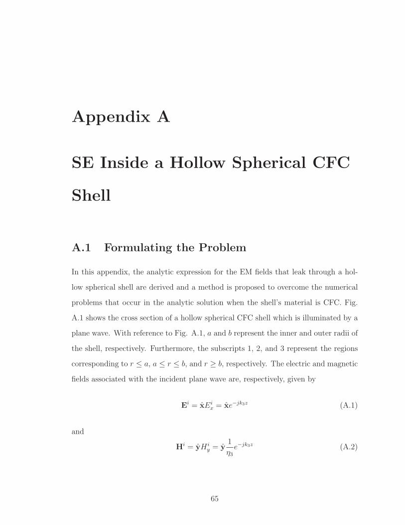
Appendix A
SE Inside a Hollow Spherical CFC
Shell
A.1 Formulating the Problem
In this appendix, the analytic expression for the EM fields that leak through a hol-
low spherical shell are derived and a method is proposed to overcome the numerical
problems that occur in the analytic solution when the shell’s material is CFC. Fig.
A.1 shows the cross section of a hollow spherical CFC shell which is illuminated by a
plane wave. With reference to Fig. A.1, a and b represent the inner and outer radii of
the shell, respectively. Furthermore, the subscripts 1, 2, and 3 represent the regions
corresponding to r ≤ a, a ≤ r ≤ b, and r ≥ b, respectively. The electric and magnetic
fields associated with the incident plane wave are, respectively, given by
Ei = xEix = xe−jk3z (A.1)
and
Hi = yH iy = y
1
η3
e−jk3z (A.2)
65

APPENDIX A. SE INSIDE A HOLLOW SPHERICAL CFC SHELL 66
Figure A.1: The cross section of a hollow spherical CFC shell which is illuminated bya plane wave. a and b represent the inner and outer radii of the shell, respectively.The subscripts 1, 2, and 3, respectively, represent the regions corresponding to r ≤ a,a ≤ r ≤ b, and r ≥ b.
where k3 and η3 are, respectively, the wavenumber and impedance of the incident
plane wave. In order to calculate the electric and magnetic fields that leak into the
shell the spherical coordinate system and the concept of electric and magnetic vector
potentials are employed [45]. The analytic solution is obtained by finding sets of
spherical wave functions that satisfy the boundary conditions at r = a and r = b.
The boundary conditions are the continuity of the tangential electric and magnetic
fields at r = a and r = b. To satisfy the boundary conditions, it is necessary and
sufficient to include TM r and TEr modes which are specified by the vector potentials
A = rAr and F = rFr, respectively. In the spherical coordinate system Ar/r and
Fr/r satisfy the following scalar Helmholtz equations [45]:
(∇2 + k2)Ar
r= 0, (A.3)
(∇2 + k2)Fr
r= 0 (A.4)
where k is the wavenumber. Therefore, the electric and magnetic vector potentials
everywhere in space should be expressed in terms of spherical wave functions that
satisfy (A.3) or (A.4) and the boundary conditions. The electric and magnetic vector
potentials in regions 1, 2, and 3 are written as follows.

APPENDIX A. SE INSIDE A HOLLOW SPHERICAL CFC SHELL 67
For region 1 i.e., 0 ≤ r ≤ a we have:
A1r =
cos φ
ωμ1
∞∑n=1
j−n 2n + 1
n(n + 1)anJn(k1r)P
1n(cos θ), (A.5)
F 1r =
sin φ
k1
∞∑n=1
j−n 2n + 1
n(n + 1)bnJn(k1r)P
1n(cos θ). (A.6)
For region 2 i.e., a ≤ r ≤ b we have:
A2r =
cos φ
ωμ2
∞∑n=1
j−n 2n + 1
n(n + 1)
[cnJn(k2r) + dnNn(k2r)
]P 1
n(cos θ), (A.7)
F 2r =
sin φ
k2
∞∑n=1
j−n 2n + 1
n(n + 1)
[enJn(k2r) + fnNn(k2r)
]P 1
n(cos θ). (A.8)
For region 3 i.e., r ≥ b we have:
A3r =
cos φ
ωμ3
∞∑n=1
j−n 2n + 1
n(n + 1)
[Jn(k3r) + gnH(2)
n (k3r)]P 1
n(cos θ), (A.9)
F 3r =
sin φ
k3
∞∑n=1
j−n 2n + 1
n(n + 1)
[Jn(k3r) + hnH
(2)n (k3r)
]P 1
n(cos θ). (A.10)
In (A.5)-(A.10) μi is the permeability of region i, ki = ω√
μiεi is the propagation
constant in region i, and εi is the complex permittivity of region i. In (A.9) and
(A.10), the incident plane wave is expressed in terms of spherical wave functions as
[45]:
Air =
cos φ
ωμ3
∞∑n=1
j−n 2n + 1
n(n + 1)Jn(k3r)P
1n(cos θ), (A.11)
F ir =
sin φ
k3
∞∑n=1
j−n 2n + 1
n(n + 1)Jn(k3r)P
1n(cos θ). (A.12)
where P 1n (cos θ) is the associated legendre function of degree n and order 1. Further-
more, in (A.5)-(A.12) Jn(.) and Nn(.) are the Schelkunoff Bessel functions of the first
and second kind and integer order n which can be expressed as [45, 46]
Jn(z) = z[fn(z) sin z + (−1)n+1f−n−1(z) cos z
](A.13)
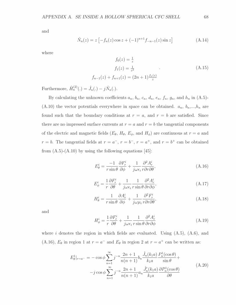
APPENDIX A. SE INSIDE A HOLLOW SPHERICAL CFC SHELL 68
and
Nn(z) = z[−fn(z) cos z + (−1)n+1f−n−1(z) sin z
](A.14)
where
f0(z) = 1z
f1(z) = 1z2
fn−1(z) + fn+1(z) = (2n + 1)fn(z)z
. (A.15)
Furthermore, H(2)n (.) = Jn(.) − jNn(.).
By calculating the unknown coefficients an, bn, cn, dn, en, fn, gn, and hn in (A.5)-
(A.10) the vector potentials everywhere in space can be obtained. an, bn,...,hn are
found such that the boundary conditions at r = a, and r = b are satisfied. Since
there are no impressed surface currents at r = a and r = b the tangential components
of the electric and magnetic fields (Eθ, Hθ, Eφ, and Hφ) are continuous at r = a and
r = b. The tangential fields at r = a−, r = b−, r = a+, and r = b+ can be obtained
from (A.5)-(A.10) by using the following equations [45]:
Eiθ =
−1
r sin θ
∂F ir
∂φ+
1
jωεi
∂2Air
r∂r∂θ, (A.16)
Eiφ =
1
r
∂F ir
∂θ+
1
jωεi
1
r sin θ
∂2Air
∂r∂φ, (A.17)
H iθ =
1
r sin θ
∂Air
∂φ+
1
jωμi
∂2F ir
r∂r∂θ, (A.18)
and
H iφ =
1
r
∂F ir
∂θ+
1
jωεi
1
r sin θ
∂2Air
∂r∂φ(A.19)
where i denotes the region in which fields are evaluated. Using (A.5), (A.6), and
(A.16), Eθ in region 1 at r = a− and Eθ in region 2 at r = a+ can be written as:
E1θ |r=a− = − cos φ
∞∑n=1
j−n 2n + 1
n(n + 1)bn
Jn(k1a)
k1a
P 1n(cos θ)
sin θ+
−j cos φ∞∑
n=1
j−n 2n + 1
n(n + 1)an
J ′n(k1a)
k1a
∂P 1n(cos θ)
∂θ
(A.20)

APPENDIX A. SE INSIDE A HOLLOW SPHERICAL CFC SHELL 69
and
E2θ |r=a+ = − cos φ
∞∑n=1
j−n 2n + 1
n(n + 1)
[en
Jn(k2a)
k2a+ fn
Nn(k2a)
k2a
]P 1
n(cos θ)
sin θ+
−j cos φ∞∑
n=1
j−n 2n + 1
n(n + 1)
[cn
J ′n(k2a)
k2a+ dn
N ′n(k2a)
k2a
]∂P 1
n(cos θ)
∂θ.
(A.21)
By imposing the boundary condition that E1θ |r=a− = E2
θ |r=a+ the following equations
are obtained:
an
J ′n(k1a)
k1a− cn
J ′n(k2a)
k2a− dn
N ′n(k2a)
k2a= 0 (A.22)
and
bn
Jn(k1a)
k1a− en
Jn(k2a)
k2a− fn
Nn(k2a)
k2a= 0. (A.23)
It is worth noting that conditions that make Eθ continuous at r = a or r = b also
make Eφ continuous at r = a or r = b. This conclusion can be extended to magnetic
fields, also. Using (A.5), (A.6), and (A.18) the magnetic fields in region 1 at r = a−
and in region 2 at r = a+ are written as
H1θ |r=a− = −sin φ
η1
∞∑n=1
j−n 2n + 1
n(n + 1)an
Jn(k1a)
k1a
P 1n(cos θ)
sin θ+
sin φ
jη1
∞∑n=1
j−n 2n + 1
n(n + 1)bn
J ′n(k1a)
k1a
∂P 1n(cos θ)
∂θ
(A.24)
and
H2θ |r=a+ = −sin φ
η2
∞∑n=1
j−n 2n + 1
n(n + 1)
[cn
Jn(k2a)
k2a+ dn
Nn(k2a)
k2a
]P 1
n(cos θ)
sin θ+
sin φ
jη2
∞∑n=1
j−n 2n + 1
n(n + 1)
[en
J ′n(k2a)
k2a+ fn
N ′n(k2a)
k2a
]∂P 1
n(cos θ)
∂θ.
(A.25)
Imposing the boundary condition that H1θ |r=a− = H2
θ |r=a+ lead to
an
Jn(k1a)
η1k1a− cn
Jn(k2a)
η2k2a− dn
Nn(k2a)
η2k2a= 0 (A.26)

APPENDIX A. SE INSIDE A HOLLOW SPHERICAL CFC SHELL 70
and
bn
J ′n(k1a)
η1k1a− en
J ′n(k2a)
η2k2a− fn
N ′n(k2a)
η2k2a= 0. (A.27)
Using (A.7), (A.8), and (A.16) Eθ in region 1 at r = b− and Eθ in region 2 at r = b+
can be written as
E2θ |r=b− = − cos φ
∞∑n=1
j−n 2n + 1
n(n + 1)
[en
Jn(k2b)
k2b+ fn
Nn(k2b)
k2b
]P 1
n(cos θ)
sin θ+
−j cos φ∞∑
n=1
j−n 2n + 1
n(n + 1)
[cn
J ′n(k2b)
k2b+ dn
N ′n(k2b)
k2b
]∂P 1
n(cos θ)
∂θ
(A.28)
and
E3θ |r=b+ = − cos φ
∞∑n=1
j−n 2n + 1
n(n + 1)
[Jn(k3b)
k3b+ hn
H(2)n (k3b)
k3b
]P 1
n(cos θ)
sin θ+
−j cos φ
∞∑n=1
j−n 2n + 1
n(n + 1)
[J ′
n(k3b)
k3b+ gn
H(2)′
n (k3b)
k3b
]∂P 1
n(cos θ)
∂θ.
(A.29)
The boundary conditions associated with the continuity of the electric fields at r = b
lead to
cn
J ′n(k2b)
k2b+ dn
N ′n(k2b)
k2b− gn
H(2)′n (k3b)
k3b− J ′
n(k3b)
k3b= 0 (A.30)
and
en
Jn(k2b)
k2b+ fn
Nn(k2b)
k2b− hn
H(2)n (k3b)
k3b− J ′
n(k3b)
k3b= 0. (A.31)
Using (A.7)-(A.10), and (A.18) the magnetic fields at r = b− and r = b+ can be
written as
H2θ |r=b− = −sin φ
η2
∞∑n=1
j−n 2n + 1
n(n + 1)
[cn
Jn(k2b)
k2b+ dn
Nn(k2b)
k2b
]P 1
n(cos θ)
sin θ+
sin φ
jη2
∞∑n=1
j−n 2n + 1
n(n + 1)
[en
J ′n(k2b)
k2b+ fn
N ′n(k2b)
k2b
]∂P 1
n(cos θ)
∂θ
(A.32)

APPENDIX A. SE INSIDE A HOLLOW SPHERICAL CFC SHELL 71
and
H3θ |r=b+ = −sin φ
η3
∞∑n=1
j−n 2n + 1
n(n + 1)
[Jn(k3b)
k3b+ gn
H(2)n (k3b)
k3b
]P 1
n(cos θ)
sin θ+
sin φ
jη3
∞∑n=1
j−n 2n + 1
n(n + 1)
[J ′
n(k3b)
k3b+ hn
H(2)′
n (k3b)
k3b
]∂P 1
n(cos θ)
∂θ.
(A.33)
The boundary conditions associated with the continuity of the magnetic fields at
r = b lead to
cn
Jn(k2b)
η2k2b+ dn
Nn(k2b)
η2k2b− gn
H(2)n (k3b)
η3k3b− Jn(k3b)
η3k3b= 0 (A.34)
and
en
J ′n(k2b)
η2k2b+ fn
N ′n(k2b)
η2k2b− hn
H(2)′n (k3b)
η3k3b− J ′
n(k3b)
η3k3b= 0. (A.35)
Now that the boundary conditions are imposed the eight unknown coefficients an,...,hn
may be determined. In the matrix form (A.22), (A.23), (A.26), (A.27), (A.30), (A.31),
(A.34), and (A.35) can be written as
⎡⎢⎢⎢⎢⎢⎢⎢⎣
J ′n(k1a)k1a
−J ′n(k2a)
k2a
−N ′n(k2a)
k2a0
Jn(k1a)η1k1a
−Jn(k2a)η2k2a
−Nn(k2a)η2k2b
0
0 J ′n(k2b)k2b
N ′n(k2b)k2b
−H(2)′n (k3b)k3b
0 Jn(k2b)η2k2b
Nn(k2b)η2k2b
−H(2)n (k3b)η3k3b
⎤⎥⎥⎥⎥⎥⎥⎥⎦
⎡⎢⎢⎢⎢⎢⎢⎢⎣
an
cn
dn
gn
⎤⎥⎥⎥⎥⎥⎥⎥⎦
=
⎡⎢⎢⎢⎢⎢⎢⎢⎣
0
0
J ′n(k3b)k3b
Jn(k3b)η3k3b
⎤⎥⎥⎥⎥⎥⎥⎥⎦
(A.36)
and ⎡⎢⎢⎢⎢⎢⎢⎢⎣
Jn(k1a)k1a
−Jn(k2a)k2a
−Nn(k2a)k2a
0
J ′n(k1a)
η1k1a
−J ′n(k2a)
η2k2a
−N ′n(k2a)
η2k2a0
0 Jn(k2b)k2b
Nn(k2b)k2b
−H(2)n (k3b)k3b
0 J ′n(k2b)
η2k2b
N ′n(k2b)
η2k2b
−H(2)′n (k3b)η3k3a
⎤⎥⎥⎥⎥⎥⎥⎥⎦
⎡⎢⎢⎢⎢⎢⎢⎢⎣
bn
en
fn
hn
⎤⎥⎥⎥⎥⎥⎥⎥⎦
=
⎡⎢⎢⎢⎢⎢⎢⎢⎣
0
0
Jn(k3b)k3b
J ′n(k3b)
η3k3a
⎤⎥⎥⎥⎥⎥⎥⎥⎦
. (A.37)
Eqs. (A.36) and (A.37) may be solved using the standard numerical methods for
solving linear systems [47]. Then, the electric and magnetic fields that leak through
the shell to the region of r ≤ a can be expressed using (A.5), (A.6), and the following
APPENDIX A. SE INSIDE A HOLLOW SPHERICAL CFC SHELL 72
equations [45]:
E1r =
1
jωε1
(k21 +
∂2
∂r2)A1
r = −j cos φ
∞∑n=1
j−n 2n + 1
n(n + 1)an
[Jn(k1r) + J ′′
n(k1r)]P 1
n(cos θ),
(A.38)
E1θ =
−1
r sin θ
∂F 1r
∂φ+
1
jωε1
∂2A1r
r∂r∂θ= − cos φ
∞∑n=1
j−n 2n + 1
n(n + 1)bn
Jn(k1r)
k1r
P 1n(cos θ)
sin θ
−j cos φ
∞∑n=1
j−n 2n + 1
n(n + 1)an
J ′n(k1r)
k1r
∂P 1n(cos θ)
∂θ,
(A.39)
E1φ =
1
r
∂F 1r
∂θ+
1
jωε1
1
r sin θ
∂2A1r
∂r∂φ= sin φ
∞∑n=1
j−n 2n + 1
n(n + 1)bn
Jn(k1r)
k1r
∂P 1n(cos θ)
∂θ
+j sin φ
∞∑n=1
j−n 2n + 1
n(n + 1)an
J ′n(k1r)
k1r
P 1n(cos θ)
sin θ,
(A.40)
H1r =
1
jωμ1
(k21+
∂2
∂r2)F 1
r =1
jη1
sin φ∞∑
n=1
j−n 2n + 1
n(n + 1)bn
[Jn(k1r) + J ′′
n(k1r)]P 1
n(cos θ),
(A.41)
H1θ =
1
r sin θ
∂A1r
∂φ+
1
jωμ1
∂2F 1r
r∂r∂θ= − sin φ
η1
∞∑n=1
j−n 2n + 1
n(n + 1)an
Jn(k1r)
k1r
P 1n(cos θ)
sin θ
+sin φ
jη1
∞∑n=1
j−n 2n + 1
n(n + 1)bn
J ′n(k1r)
k1r
∂P 1n(cos θ)
∂θ,
(A.42)
and
H1φ =
1
r
∂F 1r
∂θ+
1
jωε1
1
r sin θ
∂2A1r
∂r∂φ=− cos φ
η1
∞∑n=1
j−n 2n + 1
n(n + 1)bn
Jn(k1r)
k1r
∂P 1n(cos θ)
∂θ
+cos φ
jη1
∞∑n=1
j−n 2n + 1
n(n + 1)an
J ′n(k1r)
k1r
P 1n(cos θ)
sin θ.
(A.43)

APPENDIX A. SE INSIDE A HOLLOW SPHERICAL CFC SHELL 73
A.2 Fields at the Origin
Eqs. (A.38)-(A.43) may be used to calculate fields everywhere inside the shell. The
fields at the origin can be found using only the terms a1 and b1. Using (A.38)-(A.43)
the magnitude of the electric and magnetic fields at the origin are, respectively
limr→0
|E1(r, θ, φ)| =√
|E1r |2 + |E1
θ |2 + |E1φ|2 = |a1| (A.44)
and
limr→0
|H1(r, θ, φ)| =√|H1
r |2 + |H1θ |2 + |H1
φ|2 =|b1|η0
. (A.45)
To obtain (A.44) and (A.45) use has been made of the following limitations and
identities [46]:
limr→0
Jn(k1r)
k1r= 0, n ≥ 1, (A.46)
limr→0
J ′n(k1r)
k1r= lim
r→0J ′′
n(k1r) =
⎧⎪⎪⎨⎪⎪⎩
2/3, n = 1
0, n > 1
, (A.47)
P1(cos θ) = cos θ, (A.48)
and
P 11 (cos θ) =
∂P1(cos θ)
∂θ= − sin θ. (A.49)
A.3 Numerical Issues
Fig. A.1 shows a hollow spherical CFC shell which is illuminated by a plane wave at
the frequency of f = 100 MHz. The propagation constant in the CFC material with
σ = 104 S/m is given by [36]
k2 =
√j2πfμ0σ
j= 1986.9 − j1986.9 [rad/m]. (A.50)

APPENDIX A. SE INSIDE A HOLLOW SPHERICAL CFC SHELL 74
Using (A.50), the Schelkunoff Bessel functions Jn(k2b) and Nn(k2b) which are given
by (A.13)-(A.15) could not be evaluated for b > 35 cm even when double precision
variable are employed. This is because sin(k2b) and cos(k2b) overflow for b > 35 cm.
To eliminate this problem, an and bn are expressed in terms of sin [k2(b − a)] and
cos [k2(b − a)] as described in the following.
Using (A.36) and (A.37), an and bn can be written as
an =
∣∣∣∣∣∣∣∣∣∣∣∣∣
0 −J ′n(k2a)
k2a
−N ′n(k2a)
k2a0
0 −Jn(k2a)η2k2a
−Nn(k2a)η2k2a
0
J ′n(k3b)k3b
J ′n(k2b)k2b
N ′n(k2b)k2b
−H(2)′n (k3b)k3b
Jn(k3b)η3k3b
Jn(k2b)η2k2b
Nn(k2b)η2k2b
−H(2)n (k3b)η3k3b
∣∣∣∣∣∣∣∣∣∣∣∣∣∣∣∣∣∣∣∣∣∣∣∣∣∣
J ′n(k1a)k1a
−J ′n(k2a)
k2a
−N ′n(k2a)
k2a0
Jn(k1a)η1k1a
−Jn(k2a)η2k2a
−Nn(k2a)η2k2a
0
0 J ′n(k2b)k2b
N ′n(k2b)k2b
−H(2)′n (k3b)k3b
0 Jn(k2b)η2k2b
Nn(k2b)η2k2b
−H(2)n (k3b)η3k3b
∣∣∣∣∣∣∣∣∣∣∣∣∣
=
1jη2η3(k2ak3b)2
ΔTMn
(A.51)
and
bn =
∣∣∣∣∣∣∣∣∣∣∣∣∣
0 −Jn(k2a)k2a
−Nn(k2a)k2a
0
0 −J ′n(k2a)
η2k2a
−N ′n(k2a)
η2k2a0
Jn(k3b)k3b
Jn(k2b)k2b
Nn(k2b)k2b
−H(2)n (k3b)k3b
J ′n(k3b)
η3k3b
J ′n(k2b)
η2k2b
N ′n(k2b)
η2k2b
−H(2)′n (k3b)η3k3b
∣∣∣∣∣∣∣∣∣∣∣∣∣∣∣∣∣∣∣∣∣∣∣∣∣∣
Jn(k1a)k1a
−Jn(k2a)k2a
−Nn(k2a)k2a
0
J ′n(k1a)
η1k1a
−J ′n(k2a)
η2k2a
−N ′n(k2a)
η2k2a0
0 Jn(k2b)k2b
Nn(k2b)k2b
−H(2)n (k3b)k3b
0 J ′n(k2b)
η2k2b
N ′n(k2b)
η2k2b
−H(2)′n (k3b)η3k3b
∣∣∣∣∣∣∣∣∣∣∣∣∣
=
j
η2η3(k2ak3b)2
ΔTEn
(A.52)

APPENDIX A. SE INSIDE A HOLLOW SPHERICAL CFC SHELL 75
where
ΔTMn = − 1
η1η2k1k3(k2ab)2Jn(k1a)H(2)′
n (k3b)[Jn(k2b)N
′n(k2a) − Nn(k2b)J
′n(k2a)
]− 1
η1η3k1k3(k2ab)2Jn(k1a)H(2)
n (k3b)[J ′
n(k2a)N ′n(k2b) − N ′
n(k2a)J ′n(k2b)
]− 1
η3η2k1k3(k2ab)2J ′
n(k1a)H(2)n (k3b)
[J ′
n(k2b)Nn(k2a) − N ′n(k2b)Jn(k2a)
]− 1
η22k1k3(k2ab)2
J ′n(k1a)H(2)′
n (k3b)[Jn(k2a)Nn(k2b) − Nn(k2a)Jn(k2b)
],
(A.53)
and
ΔTEn = − 1
η2η3k1k3(k2ab)2Jn(k1a)H(2)′
n (k3b)[Jn(k2b)N
′n(k2a) − Nn(k2b)J
′n(k2a)
]− 1
η22k1k3(k2ab)2
Jn(k1a)H(2)n (k3b)
[J ′
n(k2a)N ′n(k2b) − N ′
n(k2a)J ′n(k2b)
]− 1
η1η2k1k3(k2ab)2J ′
n(k1a)H(2)n (k3b)
[J ′
n(k2b)Nn(k2a) − N ′n(k2b)Jn(k2a)
]− 1
η1η3k1k3(k2ab)2J ′
n(k1a)H(2)′
n (k3b)[Jn(k2a)Nn(k2b) − Nn(k2a)Jn(k2b)
].
(A.54)
The numerators in (A.51) and (A.52) are simplified using
W (Jn(k3b), H(2)n (k3b)) = −j (A.55)
and
W (Jn(k2a), Nn(k2a)) = 1 (A.56)
where W (., .) is the Wronskian operator [45, 46]. In order to evaluate (A.53) and
(A.54), the terms Jn(k2a), J ′n(k2a), Jn(k2b), J ′
n(k2b), Nn(k2a), N ′n(k2a), Nn(k2b),
N ′n(k2b) should not be evaluated individually. Instead the following equations should
be used:
Jn(k2a)Nn(k2b) − Nn(k2a)Jn(k2b) = k22abW 1
n(k2a, k2b), (A.57)

APPENDIX A. SE INSIDE A HOLLOW SPHERICAL CFC SHELL 76
J ′n(k2b)Nn(k2a) − N ′
n(k2b)Jn(k2a) = −k2aW 1n(k2a, k2b) + k2
2ab[W 2n(k2a, k2b)
+W 3n(k2a, k2b)],
(A.58)
Jn(k2b)N′n(k2a) − Nn(k2b)J
′n(k2a) = −k2bW
1n(k2a, k2b) + k2
2ab[W 4n(k2a, k2b)
−W 3n(k2a, k2b)],
(A.59)
and
J ′n(k2a)N ′
n(k2b) − N ′n(k2a)J ′
n(k2b) = W 1n(k2a, k2b) + k2
2ab[W 5n(k2a, k2b)+
W 6n(k2a, k2b) + W 1
n(k2a, k2b)] + k2a[W 3
n(k2a, k2b) − W 4n(k2a, k2b)
]−k2b
[W 2
n(k2a, k2b) + W 3n(k2a, k2b)
].
(A.60)
Moreover, W 1n(k2a, k2b), W 2
n(k2a, k2b),...,W6n(k2a, k2b) are given by:
W 1n(k2a, k2b) = (−1)n+1 [fn(k2a)f−n−1(k2b) − fn(k2b)f−n−1(k2a)] cos(k2b − k2a)+
[fn(k2a)fn(k2b) + f−n−1(k2a)f−n−1(k2b)] sin(k2b − k2a),
(A.61)
W 2n(k2a, k2b) = (−1)(n+1)
[f−n−1(k2a)f ′
n(k2b) − fn(k2a)f ′−n−1(k2b)
]cos [k2(b − a)]−[
f−n−1(k2a)f ′−n−1(k2b) + fn(k2a)f ′
n(k2b)]sin [k2(b − a)] ,
(A.62)
W 3n(k2a, k2b) = (−1)(n+1)
[fn(k2a)f ′
−n−1(k2b) − fn(k2b)f′−n−1(k2a)
]sin [k2(b − a)]−
[fn(k2a)f ′n(k2b) + f−n−1(k2a)f−n−1(k2b)] cos [k2(b − a)] ,
(A.63)
W 4n(k2a, k2b) = (−1)n+1
[f ′−n−1(k2a)fn(k2b) − f ′
n(k2a)f−n−1(k2b)]cos [k2(b − a)]−[
f ′−n−1(k2a)f−n−1(k2b) + f ′
n(k2a)fn(k2b)]sin [k2(b − a)] ,
(A.64)
W 5n(k2a, k2b) =
[f ′
n(k2a)f ′n(k2b) + f ′
−n−1(k2a)f ′−n−1(k2b)
]sin [k2(b − a)]
+(−1)n+1[f ′
n(k2a)f ′−n−1(k2b) − f ′
n(k2b)f′−n−1(k2a)
]cos [k2(b − a)] ,
(A.65)

APPENDIX A. SE INSIDE A HOLLOW SPHERICAL CFC SHELL 77
and
W 6n(k2a, k2b) = sin [k2(b − a)] (−1)n+1[fn(k2a)f ′
−n−1(k2b) − f ′n(k2a)f−n−1(k2b)−
f−n−1(k2a)f ′n(k2b) + f ′
−n−1(k2a)fn(k2b)]+
cos [k2(b − a)] [−fn(k2a)f ′n(k2b) + fn′(k2a)fn(k2b)−
f−n−1(k2a)f ′−n−1(k2b) + f ′
−n−1(k2a)f−n−1(k2b)].
(A.66)
Eqs. (A.61)-(A.66) are obtained by replacing (A.13)-(A.15) in (A.53) and (A.54) and
simplifying the resulting expressions using the symbolic math toolbox in MATLAB
[48].