Calculation of Dynamic Stresses using Finite Element...
14
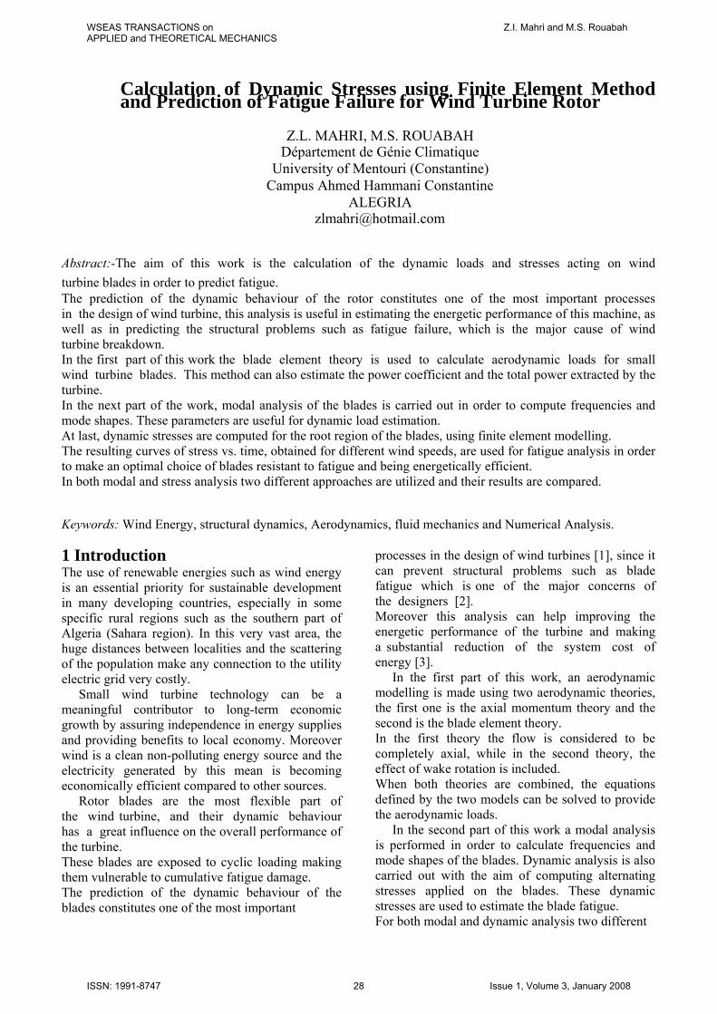
Calculation of Dynamic Stresses using Finite Element Method and Prediction of Fatigue Failure for Wind Turbine Rotor Z.L. MAHRI, M.S. ROUABAH Département de Génie Climatique University of Mentouri (Constantine) Campus Ahmed Hammani Constantine ALEGRIA [email protected] Abstract:-The aim of this work is the calculation of the dynamic loads and stresses acting on wind turbine blades in order to predict fatigue. The prediction of the dynamic behaviour of the rotor constitutes one of the most important processes in the design of wind turbine, this analysis is useful in estimating the energetic performance of this machine, as well as in predicting the structural problems such as fatigue failure, which is the major cause of wind turbine breakdown. In the first part of this work the blade element theory is used to calculate aerodynamic loads for small wind turbine blades. This method can also estimate the power coefficient and the total power extracted by the turbine. In the next part of the work, modal analysis of the blades is carried out in order to compute frequencies and mode shapes. These parameters are useful for dynamic load estimation. At last, dynamic stresses are computed for the root region of the blades, using finite element modelling. The resulting curves of stress vs. time, obtained for different wind speeds, are used for fatigue analysis in order to make an optimal choice of blades resistant to fatigue and being energetically efficient. In both modal and stress analysis two different approaches are utilized and their results are compared. Keywords: Wind Energy, structural dynamics, Aerodynamics, fluid mechanics and Numerical Analysis. 1 Introduction The use of renewable energies such as wind energy is an essential priority for sustainable development in many developing countries, especially in some specific rural regions such as the southern part of Algeria (Sahara region). In this very vast area, the huge distances between localities and the scattering of the population make any connection to the utility electric grid very costly. Small wind turbine technology can be a meaningful contributor to long-term economic growth by assuring independence in energy supplies and providing benefits to local economy. Moreover wind is a clean non-polluting energy source and the electricity generated by this mean is becoming economically efficient compared to other sources. Rotor blades are the most flexible part of the wind turbine, and their dynamic behaviour has a great influence on the overall performance of the turbine. These blades are exposed to cyclic loading making them vulnerable to cumulative fatigue damage. The prediction of the dynamic behaviour of the blades constitutes one of the most important processes in the design of wind turbines [1], since it can prevent structural problems such as blade fatigue which is one of the major concerns of the designers [2]. Moreover this analysis can help improving the energetic performance of the turbine and making a substantial reduction of the system cost of energy [3]. In the first part of this work, an aerodynamic modelling is made using two aerodynamic theories, the first one is the axial momentum theory and the second is the blade element theory. In the first theory the flow is considered to be completely axial, while in the second theory, the effect of wake rotation is included. When both theories are combined, the equations defined by the two models can be solved to provide the aerodynamic loads. In the second part of this work a modal analysis is performed in order to calculate frequencies and mode shapes of the blades. Dynamic analysis is also carried out with the aim of computing alternating stresses applied on the blades. These dynamic stresses are used to estimate the blade fatigue. For both modal and dynamic analysis two different WSEAS TRANSACTIONS on APPLIED and THEORETICAL MECHANICS Z.I. Mahri and M.S. Rouabah ISSN: 1991-8747 28 Issue 1, Volume 3, January 2008
Transcript of Calculation of Dynamic Stresses using Finite Element...
Calculation of Dynamic Stresses using Finite Element Method and Prediction of Fatigue Failure for Wind Turbine Rotor
Z.L. MAHRI, M.S. ROUABAH
Département de Génie Climatique University of Mentouri (Constantine)
Campus Ahmed Hammani Constantine ALEGRIA
Abstract:-The aim of this work is the calculation of the dynamic loads and stresses acting on wind turbine blades in order to predict fatigue. The prediction of the dynamic behaviour of the rotor constitutes one of the most important processes in the design of wind turbine, this analysis is useful in estimating the energetic performance of this machine, as well as in predicting the structural problems such as fatigue failure, which is the major cause of wind turbine breakdown. In the first part of this work the blade element theory is used to calculate aerodynamic loads for small wind turbine blades. This method can also estimate the power coefficient and the total power extracted by the turbine. In the next part of the work, modal analysis of the blades is carried out in order to compute frequencies and mode shapes. These parameters are useful for dynamic load estimation. At last, dynamic stresses are computed for the root region of the blades, using finite element modelling. The resulting curves of stress vs. time, obtained for different wind speeds, are used for fatigue analysis in order to make an optimal choice of blades resistant to fatigue and being energetically efficient. In both modal and stress analysis two different approaches are utilized and their results are compared. Keywords: Wind Energy, structural dynamics, Aerodynamics, fluid mechanics and Numerical Analysis. 1 Introduction The use of renewable energies such as wind energy is an essential priority for sustainable development in many developing countries, especially in some specific rural regions such as the southern part of Algeria (Sahara region). In this very vast area, the huge distances between localities and the scattering of the population make any connection to the utility electric grid very costly.
Small wind turbine technology can be a meaningful contributor to long-term economic growth by assuring independence in energy supplies and providing benefits to local economy. Moreover wind is a clean non-polluting energy source and the electricity generated by this mean is becoming economically efficient compared to other sources.
Rotor blades are the most flexible part of the wind turbine, and their dynamic behaviour has a great influence on the overall performance of the turbine. These blades are exposed to cyclic loading making them vulnerable to cumulative fatigue damage. The prediction of the dynamic behaviour of the blades constitutes one of the most important
processes in the design of wind turbines [1], since it can prevent structural problems such as blade fatigue which is one of the major concerns of the designers [2]. Moreover this analysis can help improving the energetic performance of the turbine and making a substantial reduction of the system cost of energy [3].
In the first part of this work, an aerodynamic modelling is made using two aerodynamic theories, the first one is the axial momentum theory and the second is the blade element theory. In the first theory the flow is considered to be completely axial, while in the second theory, the effect of wake rotation is included. When both theories are combined, the equations defined by the two models can be solved to provide the aerodynamic loads.
In the second part of this work a modal analysis is performed in order to calculate frequencies and mode shapes of the blades. Dynamic analysis is also carried out with the aim of computing alternating stresses applied on the blades. These dynamic stresses are used to estimate the blade fatigue. For both modal and dynamic analysis two different
WSEAS TRANSACTIONS onAPPLIED and THEORETICAL MECHANICS
Z.I. Mahri and M.S. Rouabah
ISSN: 1991-8747 28 Issue 1, Volume 3, January 2008
techniques are used and their results are compared. In the first approach a numerical solution of the blade motion equation is performed. In this case, a blade of simple geometry is used and considered as a continuous system. The second approach is a finite element modelling of a real blade having a complex geometry. The result of finite element modelling agrees well with that obtained by the first approach.
It should be noted that the deformation of blades depends on the Loads applied on these components. Conversely, this response to the loads (the deformation) influences the aerodynamic loads. The interaction between the load and the deformation is known as Aeroelastic phenomenon, which is one of the most challenging problems in the design and development of wind turbines. This case gives rise to a great computational complexity [4].
Finally, the fatigue of the blades is estimated in order to prevent blade breakage which is one of the major causes of wind turbine failure. However the difficulty in predicting fatigue is in large part due to an insufficient knowledge of the dynamic behaviour of the rotor [3]. 2 Aerodynamic Calculation Wind turbine aerodynamic analysis is mainly concerned with the prediction of rotor loads and power output. This analysis is one of the first and most critical steps in designing rotors and has, consequently, received a great deal of attention from a number of researchers. Because of the complexity of the unsteady three-dimensional flow field around the rotor, the use of some simplification hypotheses are necessary [5]. Different approaches are used to carry out this analysis ranging from very complex unsteady three-dimensional models to simple one dimensional analysis. So far, the blade element/momentum (BEM) formulation is the most widely used technique for such analysis, since it has demonstrated its capabilities for the conception and the design of turbines operating under normal flow conditions [6].
The objective of this part is to estimate the aerodynamic loads, which are essential to design wind systems. These loads are required for predicting and analyzing wind system energetic performance and for structural design as well. In this aerodynamic modelling two aerodynamic theories are used, the first one is the axial momentum theory and the second is the blade element theory.
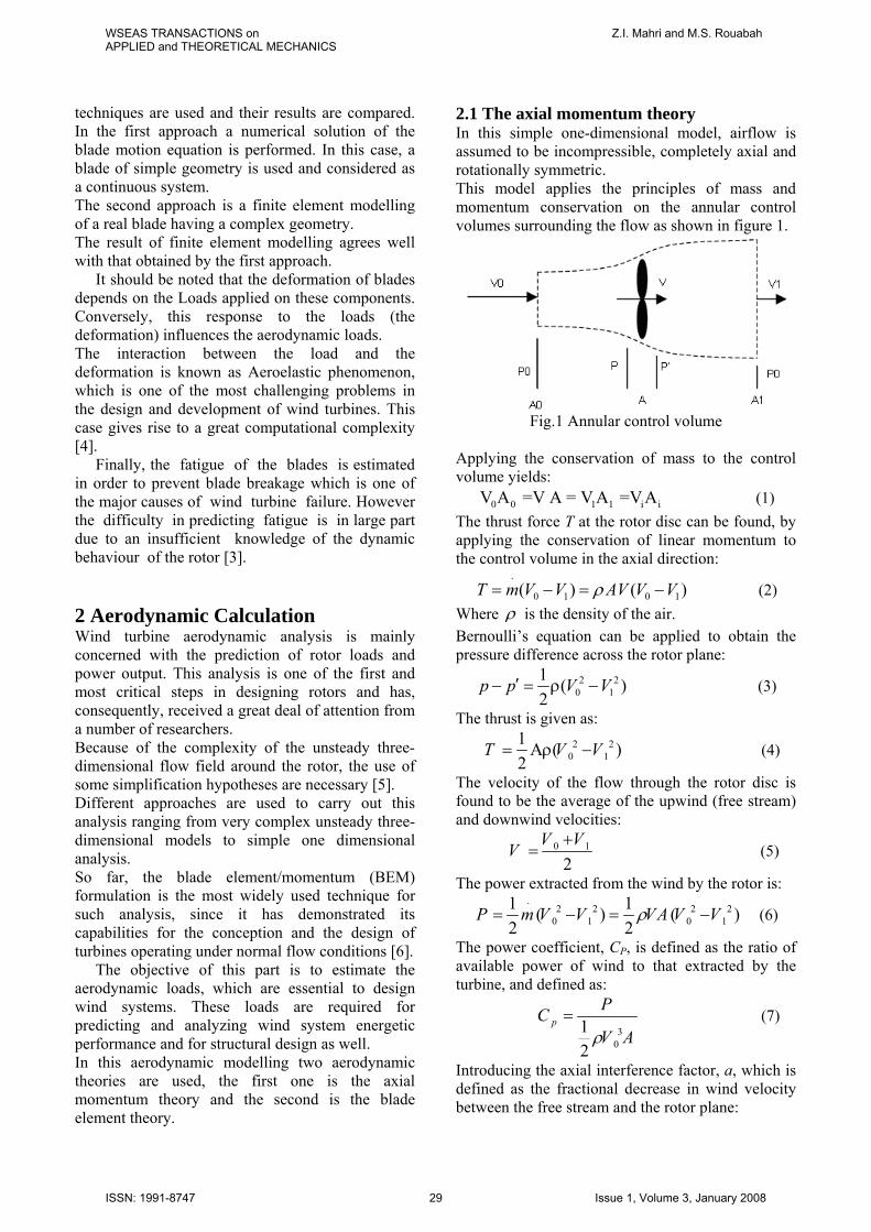
2.1 The axial momentum theory In this simple one-dimensional model, airflow is assumed to be incompressible, completely axial and rotationally symmetric. This model applies the principles of mass and momentum conservation on the annular control volumes surrounding the flow as shown in figure 1.
Fig.1 Annular control volume
Applying the conservation of mass to the control volume yields:
0 0 1 1 i iV A =V A = V A =V A (1) The thrust force T at the rotor disc can be found, by applying the conservation of linear momentum to the control volume in the axial direction:
.
0 1 0 1( ) (T m V V AV V Vρ= − = − ) (2) Where ρ is the density of the air. Bernoulli’s equation can be applied to obtain the pressure difference across the rotor plane:
2 20 1
1 (2
)p p V V′− = ρ − (3)
The thrust is given as:
2 20 1
1 (2
T V V= Αρ − ) (4)
The velocity of the flow through the rotor disc is found to be the average of the upwind (free stream) and downwind velocities:
0
2V VV 1+
= (5)
The power extracted from the wind by the rotor is: .
2 2 2 20 1 0 1
1 1( ) ( )2 2
P m V V VA V Vρ= − = − (6)
The power coefficient, CP, is defined as the ratio of available power of wind to that extracted by the turbine, and defined as:
3
012
pPCV Aρ
= (7)
Introducing the axial interference factor, a, which is defined as the fractional decrease in wind velocity between the free stream and the rotor plane:
WSEAS TRANSACTIONS onAPPLIED and THEORETICAL MECHANICS
Z.I. Mahri and M.S. Rouabah
ISSN: 1991-8747 29 Issue 1, Volume 3, January 2008
(8) 0(1 )V a= − VThe trust expression of equation (4) becomes:
20
1 4 (1 )2
T AV aρ= a− (9)
The power extracted by the rotor is: 3
01 4 (1 )2
P AV a aρ= 2−
i
(10)
The expression of Cp becomes: (11) 24 (1 )pC a a= −
2.2 The blade element theory This analysis uses the angular momentum conservation principle, taking into account the blade geometry characteristics, in order to determine the forces and the torque exerted on a wind turbine. This method is known as blade element theory [8].
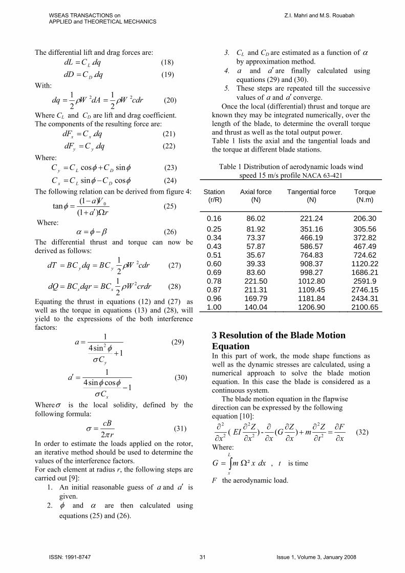
The control volume used in the previous one-dimensional model can be divided into several annular stream tube control volumes, which split the blade into a number of distinct elements, each of length dr (fig.2). In this case, the differential area of annular ring at station i, , is defined as: idA
2i idA r drπ= In this theory it is assumed that there is no interference between these blade elements and these blade elements behave as airfoils.
Fig.2 Annular stream tube control volumes
The differential rotor thrust, dT, at a given span
location on the rotor (at a specified r) can be derived from the previous theory using equation (9):
(12) 204 (1 )dT a a V rdrρ π= −
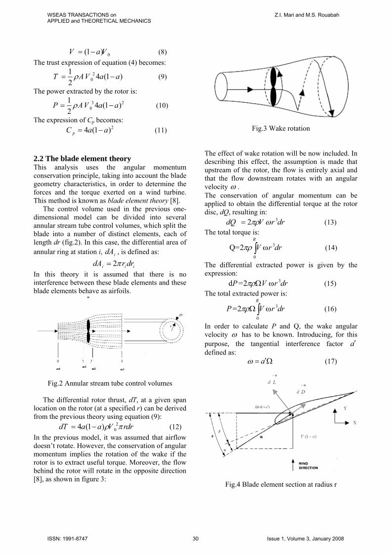
In the previous model, it was assumed that airflow doesn’t rotate. However, the conservation of angular momentum implies the rotation of the wake if the rotor is to extract useful torque. Moreover, the flow behind the rotor will rotate in the opposite direction [8], as shown in figure 3:
Fig.3 Wake rotation
The effect of wake rotation will be now included. In describing this effect, the assumption is made that upstream of the rotor, the flow is entirely axial and that the flow downstream rotates with an angular velocity ω . The conservation of angular momentum can be applied to obtain the differential torque at the rotor disc, dQ, resulting in:
32 r rdQ V dπρ ω= (13) The total torque is:
(14) 3
0
=2QR
V r drπρ ω∫The differential extracted power is given by the expression:
(15) 3d =2 V r dP πρΩ ω r
r r
The total extracted power is:
3
0
2=R
V dP πρΩ ω∫ (16)
In order to calculate P and Q, the wake angular velocity ω has to be known. Introducing, for this purpose, the tangential interference factor a′ defined as:
aω ′= Ω (17)
Fig.4 Blade element section at radius r
WSEAS TRANSACTIONS onAPPLIED and THEORETICAL MECHANICS
Z.I. Mari and M.S. Rouabah
ISSN: 1991-8747 30 Issue 1, Volume 3, January 2008
The differential lift and drag forces are: (18) .LdL C dq= (19) .DdD C dq=
With: 21 1
2 2dq W dA W cdrρ ρ= = 2 (20)
Where CL and CD are lift and drag coefficient. The components of the resulting force are:
(21) .x xdF C dq= (22) .y ydF C dq=
Where: cos siny L DC C Cφ φ= + (23)
sin cosx L DC C Cφ φ= − (24) The following relation can be derived from figure 4:
0(1 )tan(1 )
a Va r
φ −=
′+ Ω (25)
Where: α φ β= − (26)
The differential thrust and torque can now be derived as follows:
212y ydT BC dq BC W cdrρ= = (27)
212x xdQ BC dqr BC W crdrρ= = (28)
Equating the thrust in equations (12) and (27) as well as the torque in equations (13) and (28), will yield to the expressions of the both interference factors:
21
4sin 1y
a
Cφ
σ
=+
(29)
1
4sin cos 1x
a
Cφ φσ
′ =−
(30)
Whereσ is the local solidity, defined by the following formula:
2cB
rσ
π= (31)
In order to estimate the loads applied on the rotor, an iterative method should be used to determine the values of the interference factors. For each element at radius r, the following steps are carried out [9]:
1. An initial reasonable guess of a and a′ is given.
2. φ and α are then calculated using equations (25) and (26).
3. CL and CD are estimated as a function of α by approximation method.
4. and aa ′are finally calculated using equations (29) and (30).
5. These steps are repeated till the successive values of and a converge. a ′
Once the local (differential) thrust and torque are known they may be integrated numerically, over the length of the blade, to determine the overall torque and thrust as well as the total output power. Table 1 lists the axial and the tangential loads and the torque at different blade stations.
Table 1 Distribution of aerodynamic loads wind speed 15 m/s profile NACA 63-421
Station (r/R)
Axial force (N) Tangential force
(N) Torque (N.m)
0.16 86.02 221.24 206.30 0.25 81.92 351.16 305.56 0.34 73.37 466.19 372.82 0.43 57.87 586.57 467.49 0.51 35.67 764.83 724.62 0.60 39.33 908.37 1120.220.69 83.60 998.27 1686.210.78 221.50 1012.80 2591.9 0.87 211.31 1109.45 2746.150.96 169.79 1181.84 2434.311.00 140.04 1206.90 2100.65
3 Resolution of the Blade Motion Equation In this part of work, the mode shape functions as well as the dynamic stresses are calculated, using a numerical approach to solve the blade motion equation. In this case the blade is considered as a continuous system.
The blade motion equation in the flapwise direction can be expressed by the following equation [10]:
2 2 2
2 2 2( ) - ( ) Z Z ZEI G m Fx x x x t x∂ ∂ ∂ ∂ ∂ ∂
+ =∂ ∂ ∂ ∂ ∂ ∂
(32)
Where:
²L
x
G m x d= Ω∫ x , t is time
F the aerodynamic load.
WSEAS TRANSACTIONS onAPPLIED and THEORETICAL MECHANICS
Z.I. Mahri and M.S. Rouabah
ISSN: 1991-8747 31 Issue 1, Volume 3, January 2008
3.1 Resolution of the free vibration Equation (Calculation of the blade mode shapes) The modal analysis is (Calculation of the natural frequencies and the mode shapes) is an essential step that precedes the dynamic analysis.
The mode shapes can be calculated in case of free vibrations (if the blade is not exposed to external loads) using equation(32), which can be written as follows:
2 2 2
2 2 2( ) - ( ) 0Z Z ZEI G mx x x x t∂ ∂ ∂ ∂ ∂
+∂ ∂ ∂ ∂ ∂
= (33)
By taking Z=S(x). (t) ϕ and using the method of variable separation, a set of two ordinary differential equations is obtained:
2 22
2 2( ) - ( ) - d d S d dSEI G m Sdx dx dx dx
ω = 0 (34)
2
22 + = 0
tddϕ ω ϕ (35)
The boundary conditions of Eq. (34) are: At the fixed end of the blade:
Displacement = 0 (0) 0 S⇒ = (36)
Slope = 0 0dS(0)dx
⇒ = (37)
At the free end of the blade:
Bending moment = 0 0d²S(L)dx²
⇒ = (38)
Shear force = 0 03
3
dS (L)dx
⇒ = (39)
The numerical solution of (34) is complicated by its special boundary problem, having two initial values, at the fixed end (Equations (36) and (37)), and two final values, at the free end (Equations (38) and (39)). In order to start a numerical solution of Eq.(34), the
initial valuesd²S(0)
dx² and
3
3
dS (0)dx
must be known.
If a first guess of these values is made, a solution S(x) can be obtained using a numerical technique, but in this case the solution obtained doesn’t necessarily satisfy the given boundary conditions. It is obvious that different initial values will give different solutions.
It has been verified that the predictor corrector method (Adam’s formula) can solve Eq.(34) with a good convergence, while the Runge-Kutta method has failed to reach convergence [11]. In this case the Runge-Kutta method is used only as starting method.
Taking:
1 2² (0) and x
²
3
3
d S dS (0)xdx dx
= =
Also:
1 2² ( )( , )
²d S Lf x x
dx= (40)
3
1 2 3
( )( , ) dS Lg x xdx
= (41)
This boundary condition problem can then be formulated as a problem of solving a set of two equations:
1 2( , ) 0f x x = (42) 1 2( , ) 0g x x = (43)
Since the analytical expressions of the functions f and g are unknown but their numerical values are obtained by the predictor corrector method, the secant method can be used to obtain the root x1 from Eq.(40) and the root x2 from Eq. (41). This iterative Secant procedure is repeated using the new values of x1 and x2 until convergence is reached.
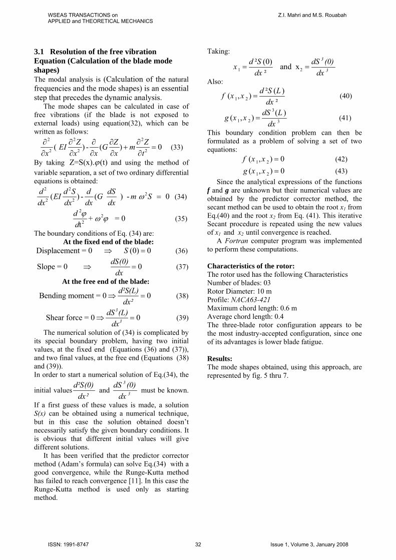
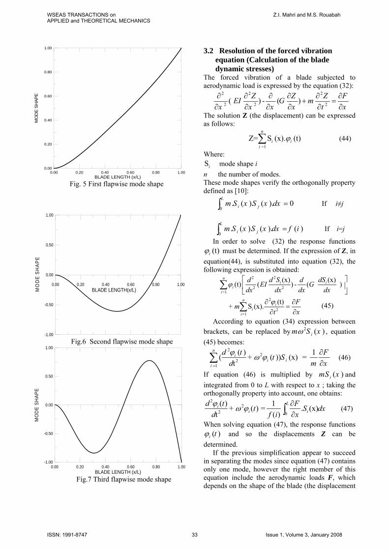
A Fortran computer program was implemented to perform these computations. Characteristics of the rotor: The rotor used has the following Characteristics Number of blades: 03 Rotor Diameter: 10 m Profile: NACA63-421 Maximum chord length: 0.6 m Average chord length: 0.4 The three-blade rotor configuration appears to be the most industry-accepted configuration, since one of its advantages is lower blade fatigue. Results: The mode shapes obtained, using this approach, are represented by fig. 5 thru 7.
WSEAS TRANSACTIONS onAPPLIED and THEORETICAL MECHANICS
Z.I. Mahri and M.S. Rouabah
ISSN: 1991-8747 32 Issue 1, Volume 3, January 2008
0.00 0.20 0.40 0.60 0.80 1.00BLADE LENGTH (x/L)
0.00
0.20
0.40
0.60
0.80
1.00
MO
DE
SHAP
E
Fig. 5 First flapwise mode shape
0.00 0.20 0.40 0.60 0.80 1.00BLADE LENGTH(x/L)
-1.00
-0.50
0.00
0.50
1.00
MO
DE
SHAP
E
Fig.6 Second flapwise mode shape
0.00 0.20 0.40 0.60 0.80 1.00BLADE LENGTH (x/L)
-1.00
-0.50
0.00
0.50
1.00
MO
DE
SHAP
E
Fig.7 Third flapwise mode shape
3.2 Resolution of the forced vibration equation (Calculation of the blade dynamic stresses)
The forced vibration of a blade subjected to aerodynamic load is expressed by the equation (32):
2 2 2
2 2 2 ( ) - ( ) Z Z ZEI G m Fx x x x t x∂ ∂ ∂ ∂ ∂ ∂
+ =∂ ∂ ∂ ∂ ∂ ∂
The solution Z (the displacement) can be expressed as follows:
(44) =1
Z= S (x). (t) n
i ii
ϕ∑Where: Si mode shape i n the number of modes. These mode shapes verify the orthogonally property defined as [10]:
0. ( ). ( ). 0
L
i jm S x S x dx =∫ If i≠j
0. ( ). ( ). ( )
L
i jm S x S x dx f i=∫ If i=j
In order to solve (32) the response functions (t)iϕ must be determined. If the expression of Z, in
equation(44), is substituted into equation (32), the following expression is obtained:
22
2 2=1
(x) (x)(t) ( ) - ( )n
i ii
i
d S dSd dEI Gdx dx dx dx
ϕ ⎡ ⎤⎢ ⎥⎣ ⎦
∑
2
2=1
(t)+ S (x).n
ii
i Fm
t xϕ∂ ∂
=∂ ∂∑ (45)
According to equation (34) expression between brackets, can be replaced by , equation 2 ( )im S xω(45) becomes:
22
21
( ) 1( + ( )) (x) = t
ni
i ii
d t Ft Sd mϕ ω ϕ
=
∂∂∑ x
(46)
If equation (46) is multiplied by and integrated from 0 to L with respect to x ; taking the orthogonally property into account, one obtains:
( )imS x
22
2 0
( ) 1+ ( ) = . (x)t ( )
Lii i
d t Ftd f i xϕ ω ϕ ∂
∂∫ S dx (47)
When solving equation (47), the response functions ( )i tϕ and so the displacements Z can be
determined. If the previous simplification appear to succeed
in separating the modes since equation (47) contains only one mode, however the right member of this equation include the aerodynamic loads F, which depends on the shape of the blade (the displacement
WSEAS TRANSACTIONS onAPPLIED and THEORETICAL MECHANICS
Z.I. Mahri and M.S. Rouabah
ISSN: 1991-8747 33 Issue 1, Volume 3, January 2008
Z) and thereby of all the modes. Thus each mode is dependent of the rest of the modes. This interdependence between the load and the shape of blade (deformation) can make the solution of equation (47) very complicated to accomplish. To start the resolution of equation (47), one should assume an initial blade form, such as a simple rigid (linear) deformation. Then the right member of this equation is computed for each mode. The equation (47) becomes:
2
22
( ) + ( ) = Cti
id t t
dϕ ω ϕ i (48)
Where Ci is the value of the right member calculated for ith
mode. Each value Ci will be supposed constant, for a small time interval ∆t. The solution of equation (48), In this case, will be [10]:
002
C (1 cos ) cos sin i t t tϕϕ ω ϕ ω ωω
′= − + +
ω (49)
Where 0ϕ and 0ϕ′ are the initial values. The new response modes calculated, using
equation (49), are used to determine the displacements Z (a new form of the blade) which allow the calculation of the aerodynamic load and thus the values Ci. This approach is repeated using the iterative formulas derived from equation (49):
1 2
C (1 cos ) cos sin jij jt t t
ϕϕ ω ϕ ω
ω ω+
′= − Δ + Δ + Δω
(50)
1C sin sin cos i
j j jt tϕ ω ωϕ ω ϕω+′ ′= Δ − Δ + tωΔ
(51) It should be noted that the subscript j, in this case, represents the calculation step number.
At the beginning, this calculation procedure is repeated, until convergence is reached (in order to correct the initial form of the blade). Afterward, this calculation is carried out for each sequential step of time [11]. The torsion motion equation is solved in a similar manner as the flapwise equation. 3.3 Resolution of the torsional motion equation (calculation of angular displacements and shear stress) The forced torsional movement is governed by the following equation [10]:
22
2( ) ALGJ C Cx x t
θ θ θ ∂∂ ∂ ∂− − Ω = −
∂ ∂ ∂ ∂x (52)
C the moment of inertia per unit length. Ω the angular velocity . θ the twist angle . LA the aerodynamic moment. G.J the torsional rigidity . The solution of this equation is form:
1
( ). ( )n
i ii
Q x tθ φ=
=∑ (53)
Q (x) the mode shape of torsion. φ (t) the response mode.
The free (natural) vibration of the torsional motion can be expressed by the following equation:
22
2( )x x
GJ C Ct
∂ ∂θ ∂ θ θ∂ ∂ ∂
0− − Ω = (54)
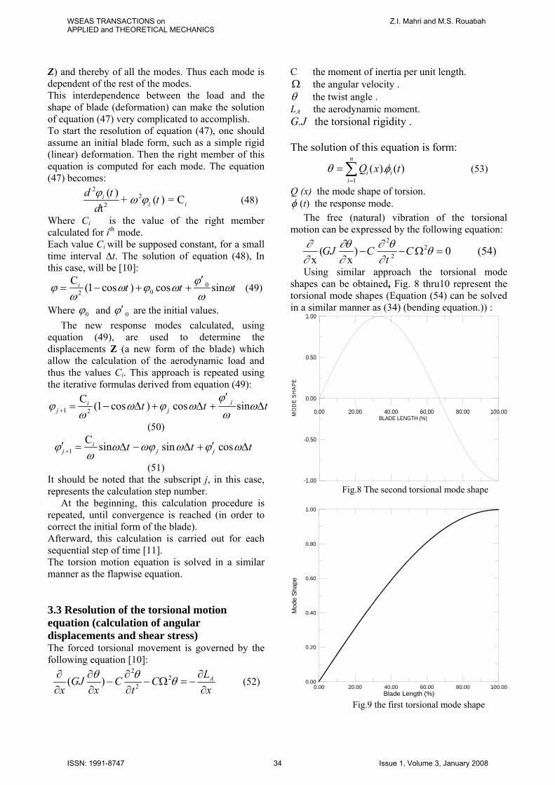
Using similar approach the torsional mode shapes can be obtained, Fig. 8 thru10 represent the torsional mode shapes (Equation (54) can be solved in a similar manner as (34) (bending equation.)) :
0.00 20.00 40.00 60.00 80.00 100.00BLADE LENGTH (%)
-1.00
-0.50
0.00
0.50
1.00
MO
DE
SHAP
E
Fig.8 The second torsional mode shape
0.00 20.00 40.00 60.00 80.00 100.00Blade Length (%)
0.00
0.20
0.40
0.60
0.80
1.00
Mod
e Sh
ape
Fig.9 the first torsional mode shape
WSEAS TRANSACTIONS onAPPLIED and THEORETICAL MECHANICS
Z.I. Mahri and M.S. Rouabah
ISSN: 1991-8747 34 Issue 1, Volume 3, January 2008
0.00 20.00 40.00 60.00 80.00 100.00Blade Length (%)
-1.00
-0.50
0.00
0.50
1.00
Mod
e Sh
ape
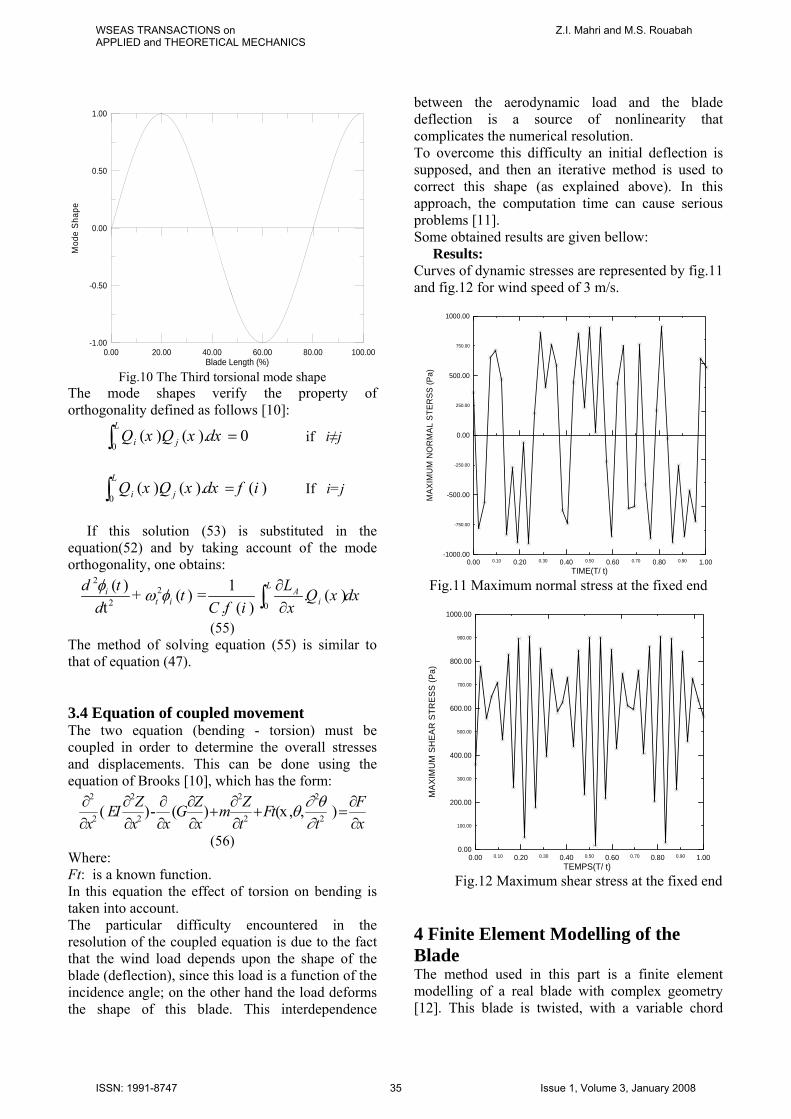
Fig.10 The Third torsional mode shape
The mode shapes verify the property of orthogonality defined as follows [10]:
0( ). ( ). 0
L
i jQ x Q x dx =∫ if i≠j
0( ). ( ). ( )
L
i jQ x Q x dx f i=∫ If i=j
If this solution (53) is substituted in the
equation(52) and by taking account of the mode orthogonality, one obtains:
22
2 0
( ) 1+ ( ) = . ( )t . ( )
Li
t i id t Lt
d C f i xφ ω φ ∂
∂∫ A Q x dx
(55) The method of solving equation (55) is similar to that of equation (47). 3.4 Equation of coupled movement The two equation (bending - torsion) must be coupled in order to determine the overall stresses and displacements. This can be done using the equation of Brooks [10], which has the form:
2 2 2 2
2 2 2 2( )- ( ) (x , , )Z Z ZEI G m Ft Fx x x x t t
∂ θθx∂
∂ ∂ ∂ ∂ ∂ ∂+ + =
∂ ∂ ∂ ∂ ∂ ∂
(56) Where: Ft: is a known function. In this equation the effect of torsion on bending is taken into account. The particular difficulty encountered in the resolution of the coupled equation is due to the fact that the wind load depends upon the shape of the blade (deflection), since this load is a function of the incidence angle; on the other hand the load deforms the shape of this blade. This interdependence
between the aerodynamic load and the blade deflection is a source of nonlinearity that complicates the numerical resolution. To overcome this difficulty an initial deflection is supposed, and then an iterative method is used to correct this shape (as explained above). In this approach, the computation time can cause serious problems [11]. Some obtained results are given bellow:
Results: Curves of dynamic stresses are represented by fig.11 and fig.12 for wind speed of 3 m/s.
0.10 0.30 0.50 0.70 0.900.00 0.20 0.40 0.60 0.80 1.00TIME(T/ t)
-750.00
-250.00
250.00
750.00
-1000.00
-500.00
0.00
500.00
1000.00
MAX
IMU
M N
OR
MAL
STE
RSS
(Pa)
Fig.11 Maximum normal stress at the fixed end
0.10 0.30 0.50 0.70 0.900.00 0.20 0.40 0.60 0.80 1.00 TEMPS(T/ t)
100.00
300.00
500.00
700.00
900.00
0.00
200.00
400.00
600.00
800.00
1000.00
MAX
IMU
M S
HEA
R S
TRES
S (P
a)
Fig.12 Maximum shear stress at the fixed end 4 Finite Element Modelling of the Blade The method used in this part is a finite element modelling of a real blade with complex geometry [12]. This blade is twisted, with a variable chord
WSEAS TRANSACTIONS onAPPLIED and THEORETICAL MECHANICS
Z.I. Mahri and M.S. Rouabah
ISSN: 1991-8747 35 Issue 1, Volume 3, January 2008
length and having a complex shape at the root region.
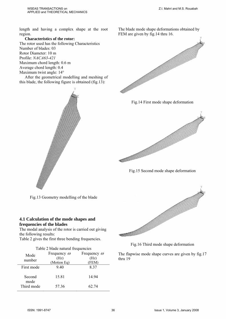
Characteristics of the rotor: The rotor used has the following Characteristics Number of blades: 03 Rotor Diameter: 10 m Profile: NACA63-421 Maximum chord length: 0.6 m Average chord length: 0.4 Maximum twist angle: 14°
After the geometrical modelling and meshing of this blade, the following figure is obtained (fig.13):
Fig.13 Geometry modelling of the blade
4.1 Calculation of the mode shapes and frequencies of the blades The modal analysis of the rotor is carried out giving the following results: Table 2 gives the first three bending frequencies.
Table 2 blade natural frequencies
Mode number
Frequency ω (Hz)
(Motion Eq)
Frequency ω (Hz)
(FEM) First mode 9.40 8.37
Second mode
15.81
14.94
Third mode 57.36 62.74
The blade mode shape deformations obtained by FEM are given by fig.14 thru 16.
Fig.14 First mode shape deformation
Fig.15 Second mode shape deformation
Fig.16 Third mode shape deformation The flapwise mode shape curves are given by fig.17 thru 19
WSEAS TRANSACTIONS onAPPLIED and THEORETICAL MECHANICS
Z.I. Mahri and M.S. Rouabah
ISSN: 1991-8747 36 Issue 1, Volume 3, January 2008
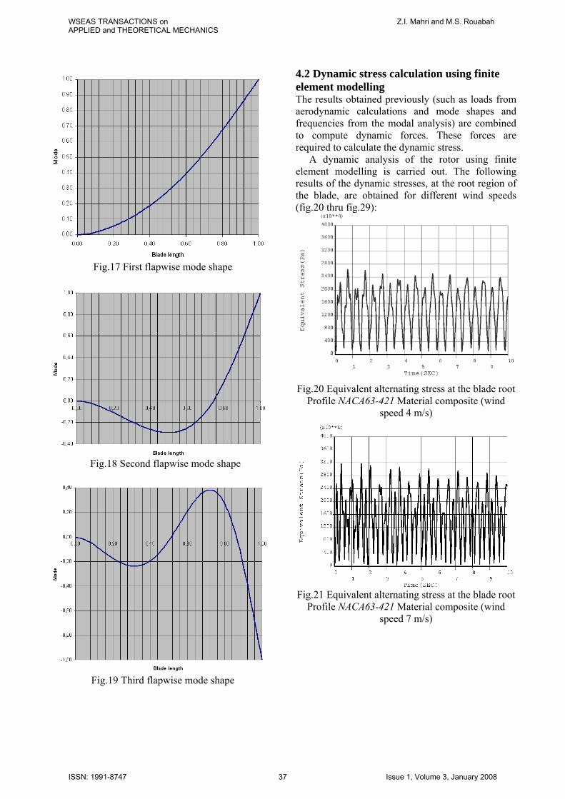
Fig.17 First flapwise mode shape
Fig.18 Second flapwise mode shape
Fig.19 Third flapwise mode shape
4.2 Dynamic stress calculation using finite element modelling The results obtained previously (such as loads from aerodynamic calculations and mode shapes and frequencies from the modal analysis) are combined to compute dynamic forces. These forces are required to calculate the dynamic stress.
A dynamic analysis of the rotor using finite element modelling is carried out. The following results of the dynamic stresses, at the root region of the blade, are obtained for different wind speeds (fig.20 thru fig.29):
Fig.20 Equivalent alternating stress at the blade root Profile NACA63-421 Material composite (wind
speed 4 m/s)
Fig.21 Equivalent alternating stress at the blade root
Profile NACA63-421 Material composite (wind speed 7 m/s)
WSEAS TRANSACTIONS onAPPLIED and THEORETICAL MECHANICS
Z.I. Mahri and M.S. Rouabah
ISSN: 1991-8747 37 Issue 1, Volume 3, January 2008
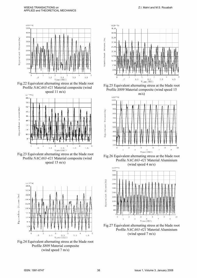
Fig.22 Equivalent alternating stress at the blade root Profile NACA63-421 Material composite (wind
speed 11 m/s)
Fig.23 Equivalent alternating stress at the blade root Profile NACA63-421 Material composite (wind
speed 15 m/s)
Fig.24 Equivalent alternating stress at the blade root
Profile S809 Material composite (wind speed 7 m/s)
Fig.25 Equivalent alternating stress at the blade root
Profile S809 Material composite (wind speed 15 m/s)
Fig.26 Equivalent alternating stress at the blade root
Profile NACA63-421 Material Aluminium (wind speed 4 m/s)
Fig.27 Equivalent alternating stress at the blade root
Profile NACA63-421 Material Aluminium (wind speed 7 m/s)
WSEAS TRANSACTIONS onAPPLIED and THEORETICAL MECHANICS
Z.I. Mahri and M.S. Rouabah
ISSN: 1991-8747 38 Issue 1, Volume 3, January 2008
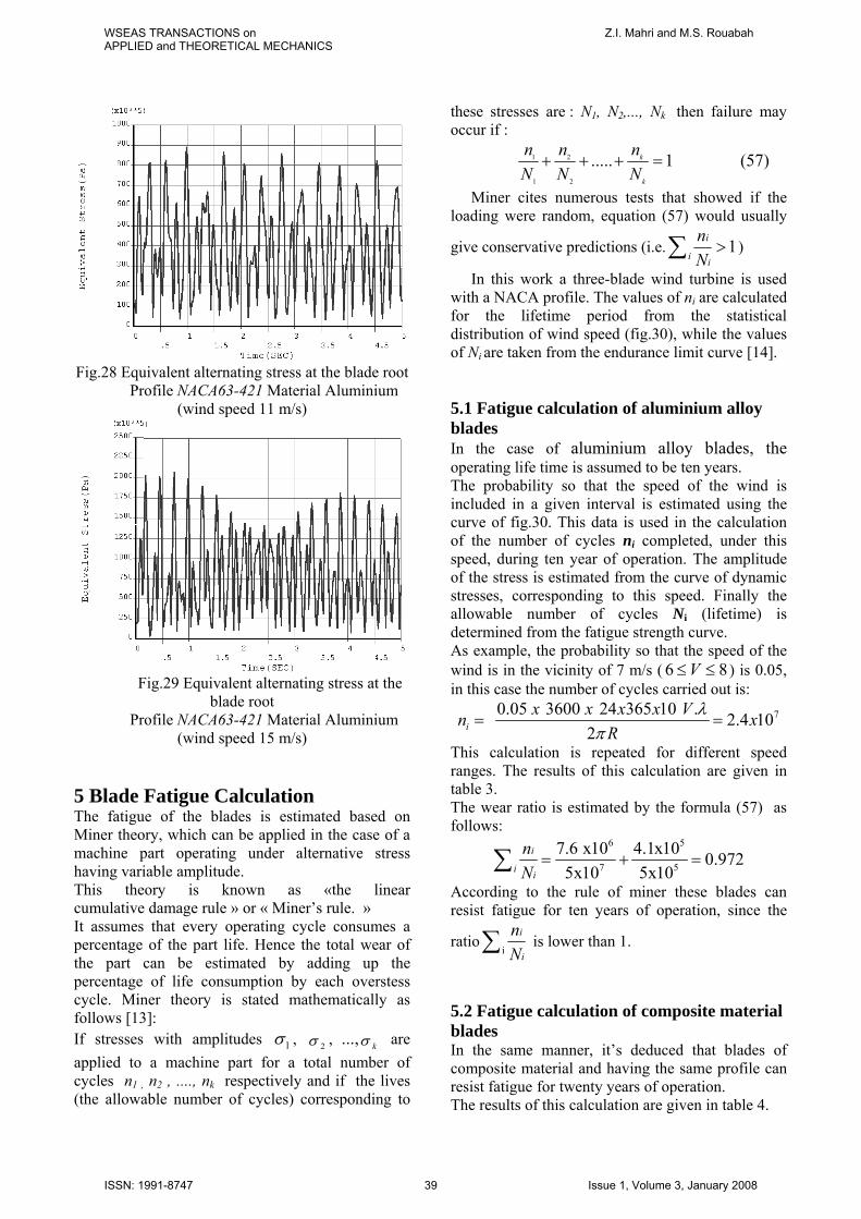
Fig.28 Equivalent alternating stress at the blade root
Profile NACA63-421 Material Aluminium (wind speed 11 m/s)
Fig.29 Equivalent alternating stress at the
blade root Profile NACA63-421 Material Aluminium
(wind speed 15 m/s) 5 Blade Fatigue Calculation The fatigue of the blades is estimated based on Miner theory, which can be applied in the case of a machine part operating under alternative stress having variable amplitude. This theory is known as «the linear cumulative damage rule » or « Miner’s rule. » It assumes that every operating cycle consumes a percentage of the part life. Hence the total wear of the part can be estimated by adding up the percentage of life consumption by each overstess cycle. Miner theory is stated mathematically as follows [13]: If stresses with amplitudes 1σ , 2σ , ..., kσ are applied to a machine part for a total number of cycles n1 , n2 , ...., nk respectively and if the lives (the allowable number of cycles) corresponding to
these stresses are : N1, N2,..., Nk then failure may occur if :
1 2
1 2
..... 1k
k
n n nN N N
+ + + = (57)
Miner cites numerous tests that showed if the loading were random, equation (57) would usually
give conservative predictions (i.e. 1i
i i
nN
>∑ )
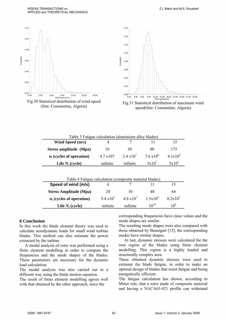
In this work a three-blade wind turbine is used with a NACA profile. The values of ni are calculated for the lifetime period from the statistical distribution of wind speed (fig.30), while the values of Ni are taken from the endurance limit curve [14]. 5.1 Fatigue calculation of aluminium alloy blades In the case of aluminium alloy blades, the operating life time is assumed to be ten years. The probability so that the speed of the wind is included in a given interval is estimated using the curve of fig.30. This data is used in the calculation of the number of cycles ni completed, under this speed, during ten year of operation. The amplitude of the stress is estimated from the curve of dynamic stresses, corresponding to this speed. Finally the allowable number of cycles Ni (lifetime) is determined from the fatigue strength curve. As example, the probability so that the speed of the wind is in the vicinity of 7 m/s ( ) is 0.05, in this case the number of cycles carried out is:
6 V≤ ≤ 8
70.05 3600 24 365 10 . 2.4 102i
x x x x Vn xR
λπ
= =
This calculation is repeated for different speed ranges. The results of this calculation are given in table 3. The wear ratio is estimated by the formula (57) as follows:
6 5
7 5
7.6 x10 4.1x10 0.9725x10 5x10
i
i i
nN
= + =∑
According to the rule of miner these blades can resist fatigue for ten years of operation, since the
ratioi
i
i
nN∑ is lower than 1.
5.2 Fatigue calculation of composite material blades In the same manner, it’s deduced that blades of composite material and having the same profile can resist fatigue for twenty years of operation. The results of this calculation are given in table 4.
WSEAS TRANSACTIONS onAPPLIED and THEORETICAL MECHANICS
Z.I. Mahri and M.S. Rouabah
ISSN: 1991-8747 39 Issue 1, Volume 3, January 2008
0.00 3.00 6.00 9.00 12.00 15.00 18.00Wind speed (m/s)
0.00
0.02
0.04
0.06
0.08
0.10
0.12
Prob
abilit
y
Fig.30 Statistical distribution of wind speed
(Site: Constantine, Algeria)
0.00 3.00 6.00 9.00 12.00 15.00 18.00 21.00 24.00 27.00 30.00Wind speed(m/s)
0.00
0.02
0.04
0.06
0.08
0.10
0.12
0.14
0.16
Prob
abilit
y
Fig.31 Statistical distribution of maximum wind
speed(Site: Constantine, Algeria)
Table 3 Fatigue calculation (aluminium alloy blades) Wind Speed (m/s) 4 7 11 15
Stress amplitude (Mpa) 10 30 80 175
ni (cycles of operation) 4.7 x10⁷ 2.4 x10⁷ 7.6 x10⁶ 4.1x10⁵
Life Ni (cycle) infinite infinite 5x10⁷ 5x10⁵
Table 4 Fatigue calculation (composite material blades) Speed of wind (m/s) 4 7 11 15
Stress Amplitude (Mpa) 24 30 40 64
ni (cycles of operation) 9.4 x10⁷ 4.8 x10⁷ 1.5x10⁶ 8.2x10⁵
Life Ni (cycle) infinite infinite 1010 108
6 Conclusion In this work the blade element theory was used to calculate aerodynamic loads for small wind turbine blades. This method can also estimate the power extracted by the turbine.
A modal analysis of rotor was performed using a finite element modelling in order to compute the frequencies and the mode shapes of the blades. These parameters are necessary for the dynamic load calculation. The modal analysis was also carried out in a different way using the blade motion equation. The result of finite element modelling agrees well with that obtained by the other approach, since the
corresponding frequencies have close values and the mode shapes are similar. The resulting mode shapes were also compared with those obtained by Baumgart [15], the corresponding modes have similar shapes.
At last, dynamic stresses were calculated for the root region of the blades using finite element modelling. This region is a highly loaded and structurally complex area. These obtained dynamic stresses were used to estimate the blade fatigue, in order to make an optimal design of blades that resist fatigue and being energetically efficient. The fatigue calculation has shown, according to Miner rule, that a rotor made of composite material and having a NACA63-421 profile can withstand
WSEAS TRANSACTIONS onAPPLIED and THEORETICAL MECHANICS
Z.I. Mahri and M.S. Rouabah
ISSN: 1991-8747 40 Issue 1, Volume 3, January 2008
fatigue failure for duration close to 20 years with an operating speed exceeding 15 m/s. In order to make conservative estimation of fatigue, one can use the statistical distribution of maximum wind speed (fig. 31)
The interdependence between the aerodynamic load and the blade deflection known as Aeroelastic phenomenon, is the most challenging problems in the design of wind turbines since it causes a great deal of computational complexity.
The minimum cost of energy is the criterion actually used to optimize blade geometry rather than maximum annual energy production. The optimization of wind turbine based on Minimum cost of energy requires a multidisciplinary method that includes aerodynamic and structural models for blades along with a cost model for the whole turbine [16]. This work can be a part of a global optimization study aiming to minimize cost and structurral problems of wind turbine while maximizing its energetic performance. References: [1] P.S. Veers, T.D. Ashwill, Trends in Design Manufacture an Evaluation of Wind Turbine, Wind Energy, Vol.6, 2003, pp. 245-259. [2] K.O. Ronoldk, Reliability-based Fatigue Design of Wind Turbine Rotor Blades, Engineering Structures, Vol.21, 1999, pp. 1101-1114. [3] F. Rasmunssen, M.H. Hansen, Present Status of Aeroelasticity of Wind Turbine, Wind Energy, Vol.6, 2003, pp.213-228. [4] P.S Veers, T.D. Ashwill, Trends in Design Manufacture and Evaluation of Wind Turbine, Wind Energy, Vol.6, 2003, pp.245-259. [5] W. Can-Xing, S. Xi, Numerical Simulation of Three Dimensional Flow in a Centrifugal Fan, WSEAS Transactions on Applied and Theoretical Mechanics, Vol.1, No.1, 2006. [6] C. Masson, A. Smaili, C. Leclerc, Aerodynamic Analysis of HAWT Operating in Unsteady Conditions, Wind Energy, Vol.4, 2001, pp1-22. [7] E. Lysen, Introduction to Wind Energy, Netherlands: Amersfort, 2nd Edition, 1983. [8] J.M. Jonkman, Modeling of the UAE Wind Turbine for Refinement of Fast Ad, National Renewable Energy Laboratory, Task No. WER3 2010 NREL/TP-500-34755, December 2003. [9] D. Wood, Design and Analysis of Small Wind Turbine, New castle Australia, University of New Castle, 2002. [10] A. Bramwell, Helicopter dynamic, Edward Arnold, New York, 1989. [11] Z.L, Mahri, M.S, Rouabah, Aeroelastic
Simulation of a Rotating Wind Turbine Blade, International Conference on Fluid Mechanics, WSEAS Press, Mexico, 2008. [12] L. Vasiliauskiene, S. Valentinavicius, A. Sapalas, Adaptive Finite Element Analysis for Solution of Complex Engineering Problems, WSEAS Transactions on Applied and Theoretical Mechanics, Vol.1, No.1, 2006. [13] M. Nielsen, G.C. Larsen, J. Mann, Wind Simulation for Extreme and Fatigue Load, Riso Laboratory, Riso-R-1437(EN), 2004. [14] H. Teodorescu, S. Vlase, D. Nicoara, Mechanical Behaviour of pre-Tensioned Glass Fiber Reinforced Composite Tubes Subjected to Internal Pressure, WSEAS Transactions on Applied and Theoretical Mechanics, Vol.2, No.2, 2007. [15] A. Baumgart, a Mathematical Model for Wind Turbine Blade, Journal of Sound and Vibration, Vol.251, 2002, pp. 1-12. [16] J.L. Tangler, The Evolution of Rotor and blade Design, American Wind Energy Conference, 2000.
WSEAS TRANSACTIONS onAPPLIED and THEORETICAL MECHANICS
Z.I. Mahri and M.S. Rouabah
ISSN: 1991-8747 41 Issue 1, Volume 3, January 2008