Version_17Mar2015

Calculating Population in GIS Prepared by Thomas J. Ballatore, Ph.D. Director, Lake Basin Action Network (LBAN) Affiliated Scientist, Center for Ecological Research, Kyoto University Visiting Researcher, International Lake Environment Committee (ILEC) Foundation Please send questions and comments to ballatore@lakebasin.org

Purpose This tutorial provides a step-by-step guide for calculating the population of a given area (a lake basin, an administrative area, etc.) in geographic information system (GIS) software. It uses the Lake Biwa drainage basin as an example but the techniques presented here are fully applicable to the basins you may be working on in your own countries. Two different datasets (GRUMP and Landscan) are used to explore various methods in calculating population. A follow-up tutorial will explore the use of WorldPop.

Checklist of Prerequisites

¨ Completion of “Delineating Lake Drainage Basins in ArcGIS” tutorial. ¨ Completion of “Calculating Areas and Lengths in ArcGIS” tutorial. ¨ Installation and activation of ArcGIS (version 10.0~10.2) including Spatial

Analyst extension. ¨ Internet access. (If you don’t have access, I can transfer the files via USB)

Preliminaries

Step 1. Creating a new map with the appropriate layers

Step 1.1. Open a new ArcMap document.

Step 1.2. Save it in C:\GIS\Basins\Biwa as Biwa_population.mxd.

Step 1.3. Add the following files from previous work in “Delineating Lake Drainage Basins in ArcGIS”:

• basin4.shp from C:\GIS\Basins\Biwa\SRTM (or whatever your “final”

lake basin shapefile was called) • SWBD_final.shp from C:\GIS\Basins\Biwa\SWBD (or whatever your final

“waterbody” shapefile was called) This is all the previously-created files we will need for the tutorial.

2

Calculating Population with GRUMP

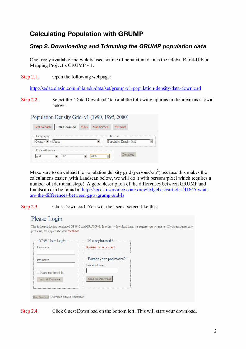
Step 2. Downloading and Trimming the GRUMP population data One freely available and widely used source of population data is the Global Rural-Urban Mapping Project’s GRUMP v.1.

Step 2.1. Open the following webpage: http://sedac.ciesin.columbia.edu/data/set/grump-v1-population-density/data-download

Step 2.2. Select the “Data Download” tab and the following options in the menu as shown below:

Make sure to download the population density grid (persons/km2) because this makes the calculations easier (with Landscan below, we will do it with persons/pixel which requires a number of additional steps). A good description of the differences between GRUMP and Landscan can be found at http://sedac.uservoice.com/knowledgebase/articles/41665-what-are-the-differences-between-gpw-grump-and-la

Step 2.3. Click Download. You will then see a screen like this:

Step 2.4. Click Guest Download on the bottom left. This will start your download.

3

This file is called jpn_grumpv1_pdens_00_grid_30.zip.

Step 2.5. Save the downloaded file (jpn_grumpv1_pdens_00_grid_30.zip) to a folder you make called C:\GIS\Data\Population\GRUMP.

Step 2.6. Unzip the file to C:\GIS\Basins\Biwa\Population\GRUMP. You should see the

following files:

Step 2.7. Add the raster jpnuds00g to the map document. You should see something like this (if you have made the basin4.shp layer outlined in black, with no fill).

This is data for all of Japan, so we would like to trim it to the Lake Biwa basin extent.

4

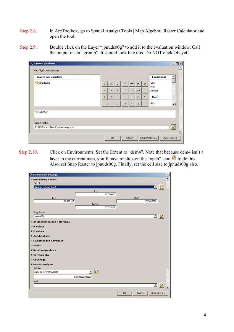
Step 2.8. In ArcToolbox, go to Spatial Analyst Tools | Map Algebra | Raster Calculator and open the tool.

Step 2.9. Double click on the Layer “jpnuds00g” to add it to the evaluation window. Call the output raster “grump”. It should look like this. Do NOT click OK yet!

Step 2.10. Click on Environments. Set the Extent to “dem4”. Note that because dem4 isn’t a layer in the current map, you’ll have to click on the “open” icon to do this. Also, set Snap Raster to jpnuds00g. Finally, set the cell size to jpnuds00g also.

5

Step 2.11. Click OK twice to evaluate the expression.

Step 2.12. Turn off the jpnuds00g layer and zoom out a bit to see that the data has indeed been trimmed to the dem4 extent.

Step 2.13. Remove jpnuds00g from the Table of Contents.

Notes. The GRUMP data is 0.00833333 degrees or 30 arc seconds which is approximately 1km2 for each pixel (but not exactly!). Next, to calculate the basin population we need to perform several steps: (1) convert the GRUMP data from floating point to integer; (2) convert the raster to feature (polygon); (3) clip the GRUMP feature with basin3.shp; (4) calculate the area of each record in the clipped shapefile; and (5) multiply the area by the population density of each record and sum to find the total population.

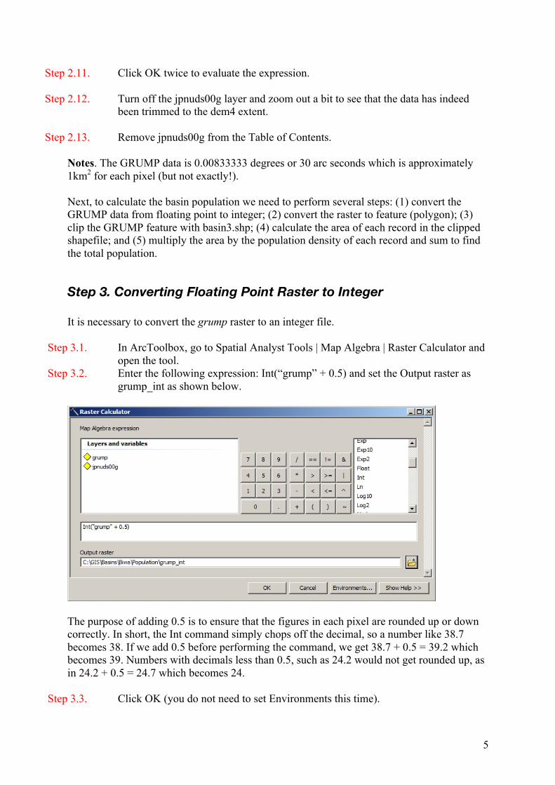
Step 3. Converting Floating Point Raster to Integer It is necessary to convert the grump raster to an integer file.

Step 3.1. In ArcToolbox, go to Spatial Analyst Tools | Map Algebra | Raster Calculator and open the tool.

Step 3.2. Enter the following expression: Int(“grump” + 0.5) and set the Output raster as grump_int as shown below.

The purpose of adding 0.5 is to ensure that the figures in each pixel are rounded up or down correctly. In short, the Int command simply chops off the decimal, so a number like 38.7 becomes 38. If we add 0.5 before performing the command, we get 38.7 + 0.5 = 39.2 which becomes 39. Numbers with decimals less than 0.5, such as 24.2 would not get rounded up, as in 24.2 + 0.5 = 24.7 which becomes 24.

Step 3.3. Click OK (you do not need to set Environments this time).

6

Step 4. Converting Raster to Polgyon Next, we must convert the raster grump_int to a polygon shapefile.

Step 4.1. In ArcToolbox, go to Conversion Tools | From Raster | Raster to Polygon and open the tool.

Step 4.2. Set grump_int as the Input raster and call the Output polygon features grump_int.shp (note you will have to type in .shp as that extension is no automatic with this tool).

Step 4.3. Click OK to get the following result:

The output shapefile probably looks a strange to you but it is okay. If you use the Identify tool to probe around, you will find that the shapefile contains the same data as the raster (but is now in a form we can do calculations on).

7

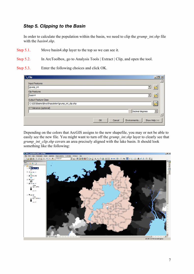
Step 5. Clipping to the Basin In order to calculate the population within the basin, we need to clip the grump_int.shp file with the basin4.shp.

Step 5.1. Move basin4.shp layer to the top so we can see it.

Step 5.2. In ArcToolbox, go to Analysis Tools | Extract | Clip, and open the tool.

Step 5.3. Enter the following choices and click OK.

Depending on the colors that ArcGIS assigns to the new shapefile, you may or not be able to easily see the new file. You might want to turn off the grump_int.shp layer to clearly see that grump_int_clip.shp covers an area precisely aligned with the lake basin. It should look something like the following:

8

Step 6. Calculating area of each record

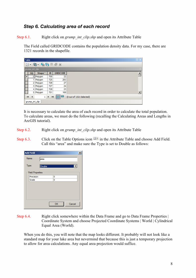
Step 6.1. Right click on grump_int_clip.shp and open its Attribute Table The Field called GRIDCODE contains the population density data. For my case, there are 1321 records in the shapefile.

It is necessary to calculate the area of each record in order to calculate the total population. To calculate areas, we must do the following (recalling the Calculating Areas and Lengths in ArcGIS tutorial).

Step 6.2. Right click on grump_int_clip.shp and open its Attribute Table

Step 6.3. Click on the Table Options icon in the Attribute Table and choose Add Field. Call this “area” and make sure the Type is set to Double as follows:

Step 6.4. Right click somewhere within the Data Frame and go to Data Frame Properties | Coordinate System and choose Projected Coordinate Systems | World | Cylindrical Equal Area (World).

When you do this, you will note that the map looks different. It probably will not look like a standard map for your lake area but nevermind that because this is just a temporary projection to allow for area calculations. Any equal area projection would suffice.

9

(Note: Instead of changing the Data Frame coordinate system, you could convert the raster by using the tool Data Management Tools | Projections and Transformations | Raster | Project Raster. This would produces a new raster but it is a complicated process that involves resampling the data and I do not do it for temporary calculations like this. For your final data---especially if you country uses a different projection (coordinate system)---you should probably do this.)

Step 6.5. In the Attribute table for grump_int_clip.shp, right click on the Area field. Choose Calculate Geometry. The Property should be “area” and the Units “Square Kilometers” as follows:

Step 6.6. Click OK and you will get the area for each record.

Step 7. Calculating total population

Step 7.1. In the Attribute Table of grump_int_clip.shp, add a new field called “pop” and be sure to make the type “Double”.

Step 7.2. Right click on that field and choose Field Calculator. You need to then multiple GRIDCODE by Area to get the population in each record (persons/km2 * km2 = persons). Your expression should look like this:

10

Step 7.3. Click OK.

Step 7.4. Right click on the top of the pop field and choose Statistics.

Step 7.5. Write down the value for Sum. In my case, it is 1,322,511 persons and represents the total number of people in the basin. Note that this is for 2000 and based on the GRUMP methodology. It also reflects the lake basin that we have delineated which may be different from what others determine (based on different pour points or elevation data). Nevertheless, it compares well with official data.

11

Calculating Population with Landscan I have found the Landscan (http://web.ornl.gov/sci/landscan/) dataset to be superior to GRUMP in many ways. However, it is not free and arranging access takes time. Assuming you/your institution is able to get access, and that you have downloaded the appropriate data, you can use this tutorial to calculate the Landscan-based population of your basin. The workflow for calculating population with Landscan is the same as for GRUMP except for one crucial difference: we first need to convert the Landscan data from “persons/pixel” to “persons/km2”. Because the area of a given pixel depends on its latitude, this is not a trivial step. Here, I will describe only the steps you need to get ready to enter the GRUMP workflow (Step 3 above).

Step L.1. Assuming you have acquired access, please unzip Landscan into a folder called C:\GIS\Data\Population\Landscan.

Step L.2. To Biwa_population.mxd, add areagrd from C:\GIS\Data\Population\Landscan\ArcGIS\AreaGrid, then add lspop2008 from C:\GIS\Data\Population\Landscan\ArcGIS\Population.

The former contains the “area of a given pixel” information; the latter contains the “persons per pixel” information. Next, we need to trim the Landscan data to the extent of dem4.

Step L.3. In ArcToolbox, go to Spatial Analyst Tools | Map Algebra | Raster Calculator and open the tool.

Step L.4. Double click on the Layer “lspop2008” to add it to the evaluation window. Call the output raster “lspop2008” in C:\GIS\Basins\Biwa\Population\Landscan (you will have to make this folder). It should look like this. Do NOT click OK yet!

12

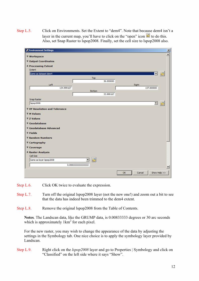
Step L.5. Click on Environments. Set the Extent to “dem4”. Note that because dem4 isn’t a

layer in the current map, you’ll have to click on the “open” icon to do this. Also, set Snap Raster to lspop2008. Finally, set the cell size to lspop2008 also.

Step L.6. Click OK twice to evaluate the expression.

Step L.7. Turn off the original lspop2008 layer (not the new one!) and zoom out a bit to see that the data has indeed been trimmed to the dem4 extent.

Step L.8. Remove the original lspop2008 from the Table of Contents.

Notes. The Landscan data, like the GRUMP data, is 0.00833333 degrees or 30 arc seconds which is approximately 1km2 for each pixel. For the new raster, you may wish to change the appearance of the data by adjusting the settings in the Symbology tab. One nice choice is to apply the symbology layer provided by Landscan.

Step L.9. Right click on the lspop2008 layer and go to Properties | Symbology and click on “Classified” on the left side where it says “Show”.

13

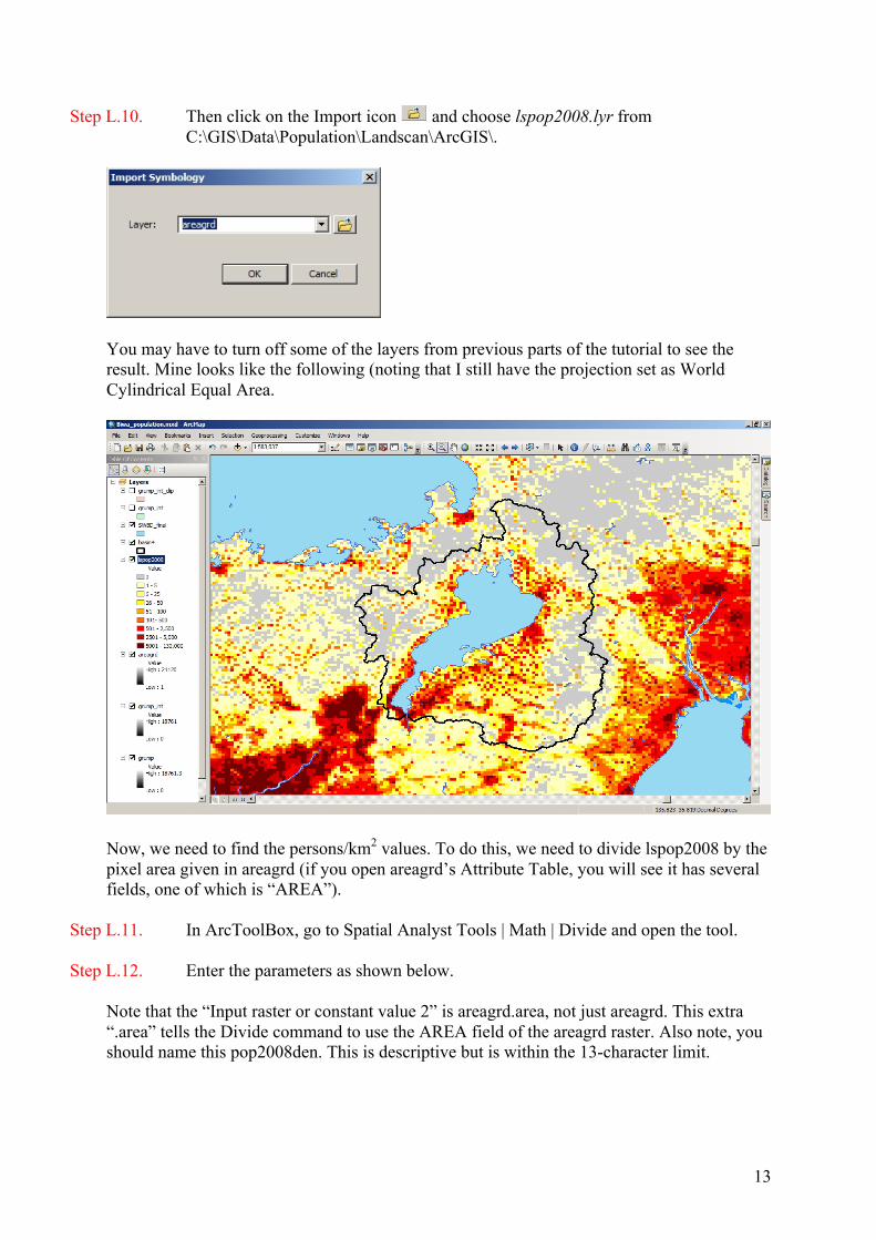
Step L.10. Then click on the Import icon and choose lspop2008.lyr from C:\GIS\Data\Population\Landscan\ArcGIS\.

You may have to turn off some of the layers from previous parts of the tutorial to see the result. Mine looks like the following (noting that I still have the projection set as World Cylindrical Equal Area.

Now, we need to find the persons/km2 values. To do this, we need to divide lspop2008 by the pixel area given in areagrd (if you open areagrd’s Attribute Table, you will see it has several fields, one of which is “AREA”).

Step L.11. In ArcToolBox, go to Spatial Analyst Tools | Math | Divide and open the tool.

Step L.12. Enter the parameters as shown below. Note that the “Input raster or constant value 2” is areagrd.area, not just areagrd. This extra “.area” tells the Divide command to use the AREA field of the areagrd raster. Also note, you should name this pop2008den. This is descriptive but is within the 13-character limit.

14

You can use the identify tool to click around on the raster to see how the pop2008den values compare with lspop2008.

Step L.13. If you like, you can change the symbology of pop2008den to be the same as lspop2008.

You will note that the colors slightly darker because the values of pop2008den are slightly higher because the area of a given pixel was less than 1 km2 on average Go to Step 3.1 on page 5 and use pop2008den instead of grump. The calculation process will be identical. I leave this as an exercise for you. For Lake Biwa, I get a value close but not the same as GRUMP. This is because the time period and methods are different so direct comparison is not possible. You can however see the higher “precision” of Landscan versus GRUMP but applying the Landscan symbology to GRUMP and comparing. Landscan uses much more auxiliary data (such as lights at night, distance from schools, roads, etc.) to allocate population within census tracks. In my experience, the results are superior to other population data sets and I recommend you try to get access if possible. Another possibility is to use the freely-available WorldPop dataset (100m!) at http://www.worldpop.org.uk/data/data_sources/ For the Lake Biwa case, the current iteration of WorldPop isn’t very accurate (somehow the road that goes around the lake has led their algorithm to allocate way too many people to the shoreline in the north). However, for work in Africa, I have found WorldPop to be superior to other sources. The 100m resolution is breathtaking when the results are correct.