Michigan State University

ECE 480 - Spring 2015

Team 10 – Tool Condition Monitoring System

Final Report

Caitlin Slicker

Richard Skrbina

Ali ElSeddik

Chris Vogler

Kyle Burgess

May 1st 2015

1

Executive Summary:

Great Lakes Controls & Engineering has identified the problem of monitoring tool wear

in a multi-spindle automatic screw machine. It is necessary to monitor the wear of a cutting tool

so as it becomes dull, it can be replaced before producing faulty parts.

Team 10 implemented a solution using an accelerometer to measure the subtle vibrations

caused by the machining process, which change with tool life. The team built an embedded

system which analyzes both the frequency and amplitude of the accelerometer’s output. The

system was calibrated based on data gathered by the team on a single spindle lathe; however, the

device can be adapted for a number of machines and purposes.

2

Acknowledgements:

Design Team 10 would like to thank Justin Walz of Great Lakes Controls Engineering for

sponsoring our project and allowing us to test at their machine shop facility, Maes Tool in

Jackson, MI. We would like to thank the employees of Maes Tool for operating the lathe,

allowing us to take data, and providing valuable insight into the project requirements. We would

like to thank Brian Wright, Gregg Mudler, and Roxxane Peacock of the ECE Shop for supplying

electronic components and allowing us to loan lab equipment for gathering data in various

machine shops. We would also like to thank Dr. Joydeep Mitra for being our facilitator and

keeping us on track during this semester. Finally, we would like to thank Dr. Timothy Grotjohn,

Dr. Lalita Udpa, and the many guest speakers in class for their inspiration and encouragement.

3

Table of Contents

1. Chapter 1: Introduction and Background .............................................................................4

1. Project Description ...................................................................................................4

2. Current Commercial Systems ..................................................................................5

3. Overview of Tool Wear ...........................................................................................5

2. Chapter 2: Exploring the Solution Space .............................................................................7

1. Senor Options...........................................................................................................7

2. Analysis and Design Decision .............................................................................. 12

3. Schedule and Project Planning.............................................................................. 15

4. Project Budget ....................................................................................................... 17

3. Chapter 3: Technical Description ..................................................................................... 18

1. Power Supplies...................................................................................................... 18

2. Sensor Interface Circuit ........................................................................................ 18

3. PWM and Filters .................................................................................................. 19

4. Comparator and Interrupt ...................................................................................... 19

5. Adjustable Band Pass Filter .................................................................................. 20

6. Prototype Implementation ..................................................................................... 22

4. Chapter 4: Testing and Validation .................................................................................... 23

1. Testing Plan and Data ........................................................................................... 23

2. Final Outcomes ..................................................................................................... 29

5. Chapter 5: Final Cost, Schedule, Summary, and Conclusions ......................................... 31

6. Appendix 1: Technical Roles ............................................................................................ 33

7. Appendix 2: Literature Review ......................................................................................... 38

8. Appendix 3: Detailed Technical Attachments .................................................................. 41

4

Chapter 1: Introduction and Background

1.1 Project Description

The purpose of this project is to detect the wear of a cutting tool used in multi-spindle

automatic screw machine. A screw machine is a metal-working machine “that continuously

creates a number of finished parts from bar stock. Bar stock advances through the spindle and is

held by a collet. It is also commonly called a bar machine. The cutting tool is gradually passed

along the surface of the rotating part.” [1].

As a cutting tool becomes dull, faulty parts are produced.

Figure 1.1 shows a part that has been manufactured using a dull

cutting tool where the radial imperfections could be visibly seen.

Currently, the factory that produces these parts depends on a

part-production counter to determine when to change a cutting

tool. The cutting operation is done using what they refer to as a

‘box’ cutting tool. After 40,000 aluminum parts are produced

using the box tool, the cutting tool is changed. However,

because of variations in materials, humidity, temperature, or even lubricant viscosity, the number

of parts a given cutting tool can produce varies from this set number. As a result, it is desirable to

have a system that can dynamically detect a dull cutting tool and indicate to the machine operator

to replace the tool.

Great Lakes Controls and Engineering detailed a number of specifications that the team’s

system must meet. First, the system must detect the wear on only one cutting tool in real time,

rejecting the noise produced from the simultaneous machining operations of the other five

cutting tools. The system needs to produce an output signal to the Programmable Logic

Controller (PLC), viewable by the machine operator, which indicates the current level of tool life

remaining. This output must be a 0-10 V signal mapping of the percent tool life remaining.

Because the system is an extension of the PLC, it must run off the same 24 V power supply.

Additionally, the entire product must not be larger than 2” x 2” x 2” in order to fit within the

machine without disrupting normal operation. The budget for volume production must not be

greater than $250.

Figure 1.1: Faulty Production Part

5

Figure 1.2: Normann Tool Condition Monitoring System

In addition to these basic qualifications, the system ought to auto-calibrate in the case of a

tool being replaced. In other words, when a machine operator receives the signal to replace the

lathe tool and does so, the system’s output to the PLC should automatically reflect this change

without needing to be reset or any other calibration. Furthermore, the environment within the

machine is very volatile where coolant and metal shavings are constantly being projected during

machining operation, and so the device must be able to withstand this environment.

1.2 Current Commercial Systems

Given that most screw machines were built over fifty years ago, there is an increasing

interest within the industry to develop systems that can detect tool life for machining processes.

Whether it is to identify how much longer a tool can be run until product imperfections occur or

the precise moment a tool fails, there are effective solutions to measure both. There are a number

of sensor and sensing systems specifically designed to accommodate most machines and

machining processes. Commercial systems include those from companies such as Nordmann,

Montronix, and Prometec. These companies provide a variety of solutions for monitoring

different parameters of tool condition including force monitoring, electric power consumption,

and acoustic emission sensing, but for a significantly expensive price. For a variety of reasons,

most of these systems could not be directly

implemented to the customer’s machine.

The team took inspiration and technical

consultancy from these companies to

produce a system adaptable to the

customer’s machine. Figure 1.2 illustrates

a Normann developed system for

monitoring tool breakage on a six-spindle

automatic lathe [2].

1.3 Overview of Tool Wear

It is necessary to first understand and quantitatively define what tool wear is. Tool life,

according to Mikell P. Groover’s Fundamentals of Modern Manufacturing, “is defined as the length

of cutting time that the tool can be used. Operating the tool until final catastrophic failure is one

6

Figure 1.3: Taylor Tool Life Equation [3]

way of defining tool life” [3]. Groover

further explains that a tool can fail from

three different causes: fracture failure,

temperature failure, and gradual wear.

Fracture failure and temperature failures

are when a cutting tool breaks due to

excessive force or high temperatures on the

tool. On the other hand, gradual wear can

either be crater wear which is caused by

the action of the chip as it is being

removed from the work surface or flank wear which results from the rubbing between the newly

generated work surface and the flank face of the cutting tool [4]. Gradual flank wear is the focus

of the project. Flank wear can be approximated using tool life according to the Taylor tool life

equation where:

𝑣𝑇𝑛 = 𝐶(𝑇𝑟𝑒𝑓𝑛)

𝑤ℎ𝑒𝑟𝑒: 𝑣: 𝑠𝑝𝑖𝑛𝑑𝑙𝑒 𝑐𝑢𝑡𝑡𝑖𝑛𝑔 𝑠𝑝𝑒𝑒𝑑, 𝑇: 𝑡𝑜𝑜𝑙 𝑙𝑖𝑓𝑒

𝑛 𝑎𝑛𝑑 𝐶 𝑑𝑒𝑝𝑒𝑛𝑑 𝑜𝑛 𝑓𝑒𝑒𝑑, 𝑑𝑒𝑝𝑡ℎ 𝑜𝑓 𝑐𝑢𝑡, 𝑤𝑜𝑟𝑘 𝑚𝑎𝑡𝑒𝑟𝑖𝑎𝑙, 𝑡𝑜𝑜𝑙𝑖𝑛𝑔, 𝑎𝑛𝑑 𝑡ℎ𝑒 𝑡𝑜𝑜𝑙 𝑙𝑖𝑓𝑒 𝑐𝑟𝑡𝑖𝑡𝑒𝑟𝑖𝑜𝑛 𝑢𝑠𝑒𝑑.

Figure 1-3 plots the cutting tool’s wear as a function of time according to Groover’s

Fundamentals of Modern Manufacturing [3]. Three regions could be seen where the tool wear

increases rapidly over the initial ‘break-in’ period, then linearly in the ‘steady-state’ wear region

and finally the cutting tool is prone to failure within the final ‘failure’ region.

The Taylor tool life equation is only a theoretical measure of a cutting tool’s tool life within

the specified parameters that are determined by prior experimentation or known published

research data. It doesn’t directly apply to the project’s development; rather, it gives the team a

measure on the effects of speed and feed rate on the operation. These relationships became vital

later in the progress of the project when testing the device at different cutting speeds.

7

Chapter 2: Exploring the Solution Space

2.1 Senor Options

When producing a system that would monitor the tool wear of an automated lathe, the

most critical component was the sensor. At the onset of this project, the team conducted

extensive research to determine what method of sensing would most effectively achieve the

overall goal. Some of the parameters taken into consideration included the sensor price,

frequency range, and feasibility. The following methods were put into a feasibility matrix before

a final selection was made.

Audio: To an experienced machine operator, there is a distinguishable audible difference

between new and used cutting tools. A tool in poor condition emits a higher amplitude and

frequency output during cutting. For this reason, this was the suggested method of tool wear

sensing by Great Lakes Controls & Engineering.

To meet the requirement of sensing a single tool on the six spindle lathe, the sensing

device must be placed 2 feet away from the lathe and should only listen to an area of 4 square

inches. To achieve this design specification, the angle of incidence must be 4.76°. To understand

how this might be accomplished, the polar patterns of microphones must be taken into

consideration. A polar pattern is coordinate plane where the sensitivity of a microphone can be

plotted relative to the angle of incidence that the sound hits [5]. Figure 2.1 shows the five

common polar patterns of microphones. In comparison, the 4.76° angle of incidence sensitivity is

shown in Figure 2.2.

Figure 2.1: Common Polar Patterns of Audio Microphones

It was determined that a purely audio solution would not be possible for several reasons.

First, by analyzing the polar patterns of most commercial microphones, a single microphone

8

would not be able to capture the sound of a single tool with

necessary accuracy. A shotgun microphone has the narrowest

polar pattern but it is still much wider than the 4.76° angle of

incidence sensitivity needed [6]. Additionally, the size of a

shotgun type microphone greatly exceeded the size

requirements for this project. Directionality could be increased

with an array of microphones, also known as beamforming,

but because of the highly resonant enclosure of the lathe,

standing and reflected waves eliminate the ability to filter out

noise in an audio recording [6] [7] [8]. The team also considered more exotic acoustic solutions

such as laser vibrometry and ultrasound but these were determined to be prohibitively expensive

and not well suited to the environment within the lathe [9].

Acoustic Emissions: Acoustic Emission (AE) is the phenomenon that under stress or

pressure, materials rapidly emit energy in the form of transient elastic waves [10]. When

irreversible deformation occurs, these vibrational waves can be measured to determine structural

properties of the material of interest. Because these high frequency waves typically range from

100 kHz to 1 MHz, AE sensors are primarily designed based on frequency and desired

bandwidth [11].

For tool monitoring, there are three methods in which AE sensors can be used. The first

type of AE sensor uses a cooling or lubricant jet as a waveguide, that is, a method of wave

transmission. The sensor is placed directly on a line directed at the cutting operation, and the

emitted waves travel through the liquid back to the sensor. The second type of AE sensor is

placed directly on the tool close to the cutting operation, thus the waves are transmitted directly

through the tool material itself. The third type simply uses air as a medium of transmission to

capture the radiation of acoustic waves when the sensor is placed in close proximity to the

operation. The Figures below are examples of these types of acoustic emission sensors [12].

Figure 2.2: Approximate Representation of

4.76° Polar Pattern

9

Figure 2.3: Types of Acoustic Emission Sensors [16]

(a) AE Hydrophone (b) Contact AE Sensor (c) AE Microphone

It was initially thought that acoustic emission testing would be the appropriate choice for

real-time tool monitoring. However, after consulting with an expert in the field of AE sensors for

tool monitoring, it was discovered that AE sensing is particularly useful in detecting tool

breakages, where short, high-amplitude spikes from fracturing can be detected quickly.

However, measuring wear over the course of a tool’s life would not be effectively achieved

through this method. Another drawback was the lack of quantitative data regarding the emitted

frequencies from the tool under different loads. It was known through research that the

frequencies detected using acoustic emissions sensors would exceed the human audible spectrum

(20 kHz) and could drift into the MHz range. Frequencies that high could present hardware and

processing issues, while choosing a sensor with the wrong frequency range could render

meaningless data. Finally, after obtaining several quotes for AE sensors, it was determined that

this method would also be outside the team’s budget.

Power Consumption: When a tool is sharp, it cuts through metal easily. As it dulls, there

is greater mechanical resistance as the tool begins to drag across the part. The machine must now

work harder to maintain the same RPM, which causes an increase in power consumption. The

life of a tool can thus be measured accurately by analyzing the power consumption during

operation. This can be applied to a wide variety of machines such as CNC mills and lathes,

machining centers and transfer lines, and grinding applications. The sensor itself works based on

the Hall Effect, which states that a current carrying conductor in a magnetic field will generate a

voltage proportional to the current and magnetic field [13]. The sensor measures this voltage

difference, called the Hall voltage, which is used to calculate the instantaneous power to the load.

10

Monitoring by power consumption provides

accurate measurements and is especially effective in

detecting tool breakages. Because sensing components

use the Hall Effect, the sensor responds to magnetic

fields and are therefore easy to install because they do

not require power lines to be modified or disrupted.

This provides a non-intrusive system that does not

interfere with the cutting operation.

Nonetheless, power sensors are not well suited

to all applications. Small cutting or drilling tools are difficult to measure because there might be

very little fluctuation in the power consumption from a good to poor tool. Also, operations that

involve common-drive spindles, such as a six-spindle lathe, cannot use power consumption as a

technique [12].

In the case of the six-spindle automatic lathe being used in this project, all six spindles

are driven by a single power supply. As a result, variations in power consumption that resulted

from any single tool would be indistinguishable from the overall power consumption of the

machine or the wear of other tools. While this would have been an ideal solution, the team

immediately ruled out this method from the selection matrix.

Force Sensing: Cutting tools are

designed to remove material from an object

based on the amount of force applied, as

shown in Figure 2.5. This applied force

increases as a tool wears out and becomes dull.

The rate at which this force increases is

heavily based upon the materials being

machined as well as the tooling material.

Therefore, the remaining tool life can be

determined by the increased force applied by a

cutting tool [12].

Figure 2.4: 3-Phase Effective Power

Measurement Unit [2]

Figure 2.5: Force Sensor Placement on Rocker Arm [22]

11

In a multi-spindle lathe, there are two applications in which force sensing can be applied

and interpreted. These methods utilize a strain gauge sensor placed on the rocker arm or the feed

rod, which controls the tool performing the cutting. These highly sensitive gauges can detect

micro or nanometer fluctuations in the tool position. The strain put on the feeding system while

this cutting process occurs is measured and as it increases over time, it can thus be translated to a

decrease in tool life. Alternatively, the gauge can also capture data regarding the moment the

cutting tool makes contact with the material to be machined. By monitoring the transient

response at the start of the cutting operation, it can be shown that there will be a difference in the

tool movement when a sharp tool is used versus a deteriorated tool. The force needed to start the

initial cut of material will increase and there will be more fluctuations in tool position as initial

contact is made between tool and part [12].

While this solution seemed to be acceptable at first, it was not cost effective. Strain

sensors designed for this application were not available to stay within the team budget.

Ultimately force sensing was ruled out for this reason.

Accelerometer: An accelerometer is a device which measures g-force, or the force of

gravity. It will measure 9.81m/s2 while stationary and zero while in free-fall. The output is a

continuous voltage that is proportional to the g-force experienced by the accelerometer. For

example, the sensitivity of accelerometers can be denoted as 50 mV/g or 100 mV/g.

Accelerometers can use piezoelectric (internal crystals respond to stress), piezoresistive

(resistance changes based on force applied), or piezocapacitive (capacitance between

microstructures changes based on accelerative force applied) principles to measure changes in

acceleration [14]. An accelerometer can be an inexpensive, general-purpose solution to

measuring internal vibrations within a solid. The frequencies measured are typically lower, from

10 Hz to 30 kHz. Accelerometers are not inaccurate; rather they are most effective for large-scale

operations.

In relation to tool monitoring, there are two design solutions in which an accelerometer

can be used. The first design measures the vibration of the tool as it is in use. The accelerometer

would be mounted as close as possible to the cutting operation. The accelerometer is a pure

transducer, meaning the output is a voltage with a frequency equivalent to the vibrations

produced by the cutting operation. This data would be recorded for both good and poor condition

12

tools, and the harmonic frequency differences could create criteria in which to compare future

tools. The second design solution is concerned with the transient response of the tool as it makes

initial contact with the part being machined. Similar to force measurements, these vibrations

should intensify as the tool becomes dull, because there is an increased resistance. Therefore,

when initial contact occurs, a good tool will begin removing material quickly while a poor tool

will experience a larger “bounce back” effect before cutting, resulting in increased vibrations.

Sensor Selection: Many sensing options were available for the monitoring of tool wear.

However, these options were either not applicable to the specific process or machine specified by

Great Lakes Controls and Engineering, or were beyond the allotted budget. Based on the team’s

understanding of commercial tool monitoring sensors, it was decided that a general purpose

accelerometer would measure similar metrics related to tool wear as other commercial options,

but at a lower cost. As discussed earlier, the team used the design selection matrix shown below

in Table 2.1 to rank each sensor by criteria. While not being the top solution, an accelerometer

offered simplicity, affordability, and an overall lower risk than other sensors.

Engineering Criteria Importance Possible Solutions

Force Accelerometer AE Coolant Microphone Power

Sensitivity to Noise 3 9 3 3 3 1 9

Installation 2 3 3 3 1 3 9

Durability 1 9 9 9 3 3 9

Data Correlation to

Tool Life

5 9 3 5 3 1 3

Output Compatibility 4 3 3 3 3 3 9

Price 2 1 9 1 1 3 1

Total 101 78 63 43 35 107

Table 2.1: Solutions Selection Matrix for Tool Monitoring Sensors

2.2 Analysis and Design Decision

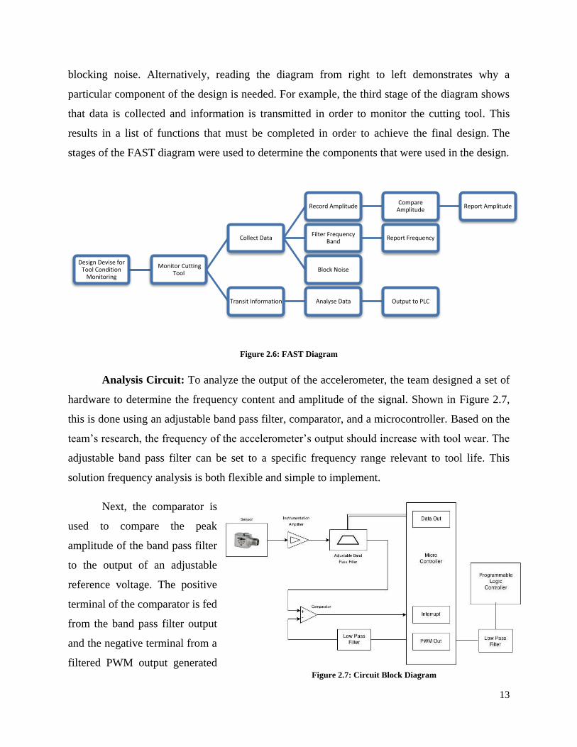
FAST Analysis: The project’s FAST diagram, shown in Figure 2.6, represents the

functions that need be completed to reach the final design. On the left is the design goal, to

design a device for tool condition monitoring. Reading the diagram from left to right

demonstrates how these functions relate to one another. For example, the third stage of the

diagram shows that data is collected by recording amplitude, filtering frequency bands, and

13

blocking noise. Alternatively, reading the diagram from right to left demonstrates why a

particular component of the design is needed. For example, the third stage of the diagram shows

that data is collected and information is transmitted in order to monitor the cutting tool. This

results in a list of functions that must be completed in order to achieve the final design. The

stages of the FAST diagram were used to determine the components that were used in the design.

Figure 2.6: FAST Diagram

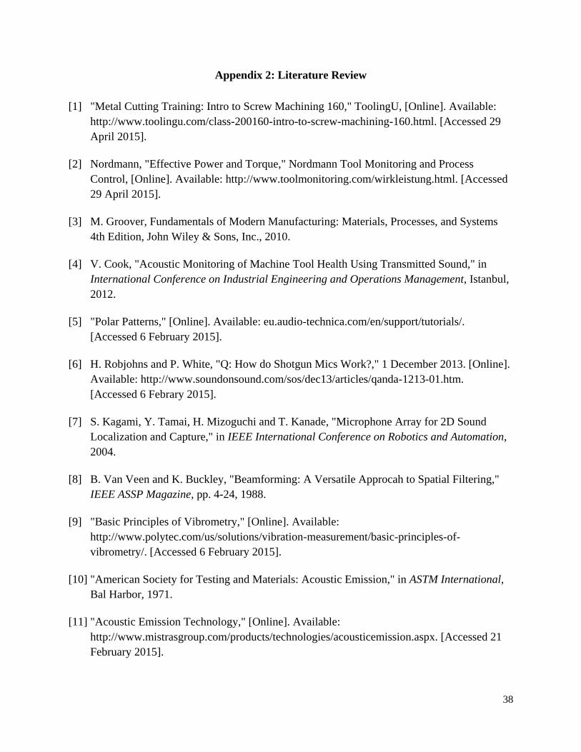
Analysis Circuit: To analyze the output of the accelerometer, the team designed a set of

hardware to determine the frequency content and amplitude of the signal. Shown in Figure 2.7,

this is done using an adjustable band pass filter, comparator, and a microcontroller. Based on the

team’s research, the frequency of the accelerometer’s output should increase with tool wear. The

adjustable band pass filter can be set to a specific frequency range relevant to tool life. This

solution frequency analysis is both flexible and simple to implement.

Next, the comparator is

used to compare the peak

amplitude of the band pass filter

to the output of an adjustable

reference voltage. The positive

terminal of the comparator is fed

from the band pass filter output

and the negative terminal from a

filtered PWM output generated

Design Devise for Tool Condition

Monitoring

Monitor Cutting Tool

Collect Data

Record Amplitude Compare

Amplitude Report Amplitude

Filter Frequency Band

Report Frequency

Block Noise

Transit Information Analyse Data Output to PLC

Figure 2.7: Circuit Block Diagram

14

from the microcontroller. If the amplitude of the filter output surpasses the reference voltage, the

comparator output will be driven high, indicating that the magnitude of the signal at a set

frequency has surpassed a reasonable level. Otherwise, the comparator output will remain low.

The output of the comparator drives an interrupt enabled pin on the microcontroller,

indicating that a milestone in tool life has been reached. Within the interrupt service routine, the

pass band of the filter and the PWM reference voltage can be adjusted to check for the next

relevant condition and the output to the PLC can be adjusted to reflect the current level of wear.

Part Selection: The accelerometer chosen was made by Connection Technology Center,

Inc.. The sensor has a rating of 100 mV/g, meaning that for each multiple of gravity acceleration

it detects, it will output a voltage 100 mV above or below the signal ground. It can detect up to

+/- 50g of acceleration.

The chosen design requires multiple band pass filters built for each frequency that is

determined to indicate tool wear. However, this implementation is labor intensive, spatially

inefficient, and inflexible. Instead, the team used a MAX262 chip, an adjustable band pass filter

IC made by Maxim Integrated. This allowed the team to filter a wide range of frequencies using

only one chip.

The MAX262 chip has switched capacitor filters whose cutoff frequency can be changed

by software control. The MAX262 has the option to change both the cutoff frequency and filter

quality for two on chip filter sections. The chip also provides high pass, low pass, band pass and

notch filter outputs for each individually adjustable filter section based on the parameters

provided by the microcontroller. The filter sections can be cascaded in order to provide sharper

filtering. The MAX262 can have a cutoff frequency from 0 - 140 kHz and costs around $15.

The microcontroller chosen was the MSP430. The MSP430 is a low power, inexpensive

microcontroller manufactured by Texas Instruments. It has the advantages of being simple to

program and interface with.

Critical Customer Specifications: The team believes that this design meets a great deal

of the customer’s specifications. As per the project description, this system design should be able

to detect the wear on a single tool during machine operation. The hardware built to interface with

15

the sensor and analyze its output will be able to produce a 0 to 10 V signal based on the sensor

output and be run off of a 24 V power supply. The system will also be capable of the necessary

auto calibration; if it is reset after a tool is replaced, the system will begin checking for the first

signs of tool wear again. The sensor is also robust enough to withstand the harsh environment

within the lathe.

The specifications that weren’t met were discussed and negotiated with the customer. For

example, the project description stated that the sensor should be 2” x 2” x 2” and attached to a

back wall of the machine, 4’ from the lathe operation. This specification was given because the

customer envisioned a solution using an acoustic microphone. After reviewing the team’s

research with the customer, it was determined that the dimensions and placement specified were

negotiable in the circumstance of a promising alternative sensing method. Additionally, the 2” x

2” x 2” size requirement pertains to the size of the elements being placed within the lathe, and

does not apply to external circuitry.

2.3 Schedule and Project Planning

One of the primary hurdles of this project was designing a system around data that would

not be available until after the system was built to gather the data. One way the team chose to

handle this, was to build a system that was flexible and could be adjusted based on the data

gathered. By using an adjustable filter IC instead of a single filter or set of filters, it was simple

to adjust the frequency band and amplitude based on what differences the team found indicated

tool wear. Additionally, a state machine in the interrupt service routine allowed the team to

check for specific conditions of interest rather than assuming that the sensor output would map

directly to the output to the PLC.

Particularly given the time constraints of the semester, it was critical that the team built a

system that could be adapted based on the data that was found to indicate differences between a

good and bad tool. This significantly reduced the critical path for the project timeline; instead of

waiting to have data to begin building a circuit around the sensor, a system could built

simultaneously and variables altered in software later based on the findings.

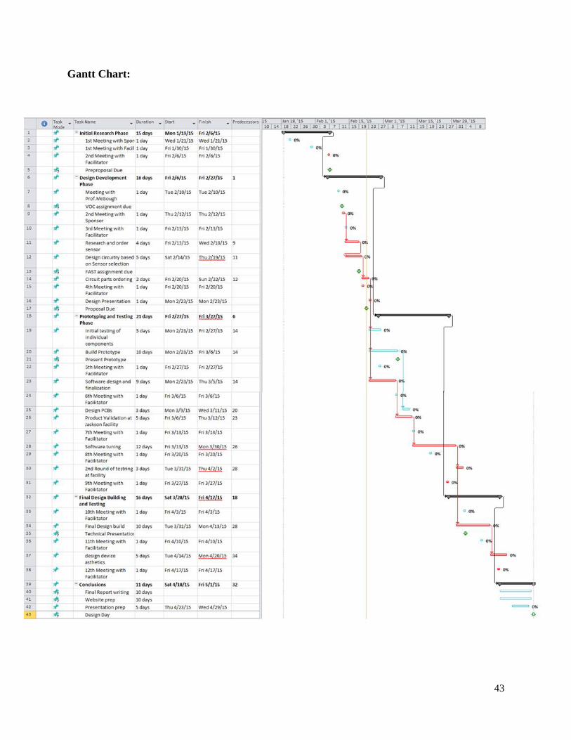
The project as a whole was divided into multiple work phases that identify the tasks

required within the project. A Gantt chart with the various tasks and work phases was built to

16

visualize these tasks and assure the work progress is on time. The Gantt chart was developed at

the early stages of the project where the final design details were unknown; hence, most of the

tasks are in general terms. The Gantt chart can be found in Appendix 3.

The following are descriptions of the 5 phases of the project:

Phase 1: Initial Research Phase: This phase included the initial meetings with the

customer and the development of the customer needs and constraints. This also introduced the

team members to each other and assigned different roles for each member.

Phase 2: Design Development Phase: This phase included looking at possible design

solutions and making decisions on parts on components for the design. This phase included

meetings with different faculty of the MSU College of Engineering, Dr. Robert McGough and

Dr. Thompson, for their consultancy on different design approaches. During this phase, the

initial circuit design was developed and the sensor selection was made. All required parts were

ordered. Finally this phase included the development of the Project Proposal to the customer

with finalized device design selections.

Phase 3: Prototyping and Testing Phase: After all parts were ordered, this phase

included building the circuits and systems for the prototype and testing individual systems

separately. The sensor power-supply circuit was built which then allowed the sensor to be tested

within the laboratory. This phase also included the development of the software for the

controlling the band-pass filter and PWM outputs, which was also tested separately within the

laboratory.

Phase 4: Final Design Building Phase: This phase was focused on compiling various

hardware sections and debugging the project as a single unit. This allowed the team to then run

different tests on the device at different machine shops at MSU and at the customer’s shop.

Lastly, the final components were housed within a presentable layout for the customer.

Phase 5: Conclusions Phase: This phase spanned the duration of the last week, and

included working on the technical communications tasks including the final report, final

presentation and demo, design day poster and the website.

17

2. 4 Project Budget

According to the ECE 480 course description, each team was granted a $500 budget to

complete their project. Great Lakes Control & Engineering also set a $250 per unit cost on each

sensing system developed. The final cost of the project is broken up into several categories in

which specific components are itemized. They are namely the sensor, microcontroller, and

analog circuitry. After completing research, it was determined that the bulk of the budget for this

system should be invested in a high-quality, durable accelerometer. To the team’s benefit, the

unit selected only consumed a third of the total available budget. Also, by utilizing the ECE shop

inventory, many hardware components could be obtained for free, thus resulting in an overall

cost savings. A detailed breakdown of the budget is displayed below in Table 2.2.

Component Quantity Price Subtotal

MSP430 1 $0.00 $0.00

PIC32 Pinguino Microcontroller 1 $16.70 $16.70

MAX262 Programmable Filter 4 $16.48 $66.58

CTC AC130 Accelerometer 1 $150.00 $150.00

Accelerometer shielded cable 1 $57.50 $57.50

Accelerometer mounting disk 1 $6.50 $6.50

20 pin SIL socket 4 $1.89 $7.56

Breadboard, resistors, capacitors, voltage

regulator, wire - $0.00 $0.00

Shipping - $13.52 $13.52

Total $318.36

Table 2.2: Itemized Cost of all Components Used

18

Chapter 3: Technical Description

The hardware and software elements of the project overlap significantly and were

developed in conjunction. While some elements, such as the power supplies, are strictly analog,

others have both hardware and software components to their implementation, such as the

MAX262 filter IC which processes an analog signal based on programmable parameters. For this

reason, this section is structured around each of the primary project elements. Each of these

sections describes both the hardware and software efforts needed to implement that element, the

schematics of which can be found in Appendix 3.

The team chose the MSP430 to control the digital elements of our circuitry. The main

functions of the MSP430 software were to program the MAX262 adjustable band pass filter IC,

output two PWM signals for the comparator and the final output, and to trigger an interrupt that

would reprogram the filter and PWMs based on the output of the comparator.

3. 1 Power Supplies

The device is powered from the lathe’s Programmable Logic Controller with 24V. This

needed to be stepped down to several other levels required by the circuitry. The voltages required

are 19V, 5V, and 3.3V. The 19 V supply powers the sensor and most of the analog circuitry. This

supply is created with an LM317 adjustable voltage regulator. The voltage output of the LM317

is a function of two resistors used to adjust the voltage. These were chosen to have an output of

19V. Fixed linear voltage regulators are used to create the 5V and 3.3V supplies. The supplies

are cascaded to minimize dropout voltage across the regulators themselves. This configuration

cuts down on the power dissipated as heat. The 5V supply is necessary for the adjustable band

pass filter chip, while the 3.3V is used for the microcontroller. There are filter capacitors

throughout the power supply to ensure clean supply rails.

3.2 Sensor Interface Circuit

The sensor requires a constant current power supply with a voltage of 18 – 30 V. The

power supply circuit given in the application notes of the sensor, and shown in Figure 3.1, calls

for a constant current diode with a current between 2 mA and 10 mA. Since constant current

diodes as a discrete component are an obscure part, the team chose to implement one with a

19

JFET transistor and resistor. The value of

the resistor was first calculated and

simulated in PSPICE before being tested

with the sensor.

3.3 PWM and DC Filters

There are two adjustable voltages

required by the circuit. The first is the

previously discussed adjustable level

used to set a comparator threshold. The

other is the overall output of the system, the 0-10V signal used to communicate the remaining

tool life with the lathe’s Programmable Logic Controller.

These adjustable voltage levels are implemented by filtering two PWM outputs of the

microcontroller. The low pass filters were implemented as second order active filters using op-

amps in a modified non-inverting amplifier configuration. An LM324 quad op-amp is used to

implement these filters.

The gain of each filter was determined by the desired output range of the voltage level.

For the signal going to the comparator, a gain of 1.8 was chosen to allow for a voltage output

range of 0 – 6V. This range overlaps well with the output of the filter IC, which is 5V. For the

overall output PWM filter, a gain of 3 was chosen, yielding a range of approximately 0 – 9.9V.

In general, the output voltage can be estimated using the formula:

𝑉𝑜𝑢𝑡 = 3.3 × 𝑔𝑎𝑖𝑛 × 𝑑𝑢𝑡𝑦 𝑐𝑦𝑐𝑙𝑒

0 ≤ 𝑑𝑢𝑡𝑦 𝑐𝑦𝑐𝑙𝑒 ≤ 1

3.4 Comparator and Interrupt

A single op-amp in an LM339 quad op-amp chip is used in our circuit for the comparator.

The comparator circuit is very simple, using only 3 resistors. A pull-up resistor is necessary for

the LM339 to saturate. The other two resistors form a voltage divider to step the saturated output

of 19V down to 3.3V, so it can interrupt the microcontroller without risk of damage to the chip.

Figure 3.1: Sensor Interface Circuit

20

When the output of the comparator goes high, indicating that the amplitude of the filter

output has surpassed the PWM reference voltage, the rising edge triggers an interrupt on the

MSP430. In order to change the values of the PWM outputs and the frequency band of the filter

during operation in response to increased tool wear, the team have implemented an interrupt

service routine (ISR) to reprogram these values when the previous conditions for amplitude and

frequency have been met.

Once inside the ISR, there is a state machine that can set the filter and PWM values to

check for a new frequency and amplitude. Designing the system in this way allows us to program

the system to check for particular conditions rather than mapping the output of the sensor

directly onto the signal to the PLC.

3.5 Adjustable Band Pass Filter

The team opted to use the MAX262

programmable switched capacitor filter IC for this

design. This chip offers a wide range of center

frequencies and bandwidths selected under

microprocessor control. The chip provides output for

low pass, band pass, and high pass based on the

parameters given. The center frequency is determined

as a function of the external clock frequency and a

selected pre-defined ratio based on the internal register

value set in software.

The chip can be powered with a +/-5V supply,

or a single ended +5V supply. The team opted to use a

single 5V supply to avoid the need for negative voltages. In this configuration, the ground pin is

biased at +2.5V, and the negative supply is grounded. Thus, any signal fed into the filter should

have a DC offset of 2.5V, and the output of the filter has this same offset. There are some

drawbacks to running the filter off of a single ended supply, including a large amount of error in

the clock to center frequency ratios supplied in the datasheet. The datasheet does not supply

Figure 3.2: Filter Parameter Equations

21

Figure 3.3: Description of MAX262 Address Space and Storage

much information on how the ratios change, and when running in this mode, trial and error is the

best method of getting the desired filter parameters.

The team chose to clock the MAX262 with a 1 MHz crystal oscillator. The crystal

oscillator requires only a 5V power supply to output a 50% duty cycle square wave with great

accuracy. A clock frequency of 1 MHz gives provides a center frequency range from around 7.2

kHz to 25.8 kHz. The team determined that this frequency range overlapped well with the data

gathered from good and bad cutting tools.

To program the MAX262 chip, the correct data correlating to a specific center frequency

and pass band must be determined, then the data must be sent to the chip through a series of

write operations. The equations in Figure 3.2 show the basic method for calculating filter values.

Once the desired output has been calculated, the correct data to be sent to the filter can be

determined from the data sheet. The actual center frequency of the chip is a function of the input

clock to the filter and so it must be calculated in conjunction with this value.

Figure 3.4: MAX262 Timing Diagram

22

The MAX262 chip uses seven parallel inputs to receive data and set the center frequency

and pass band for the two on chip filters. Of these seven pins, two are data inputs, four are

address bits, and one is a write enable line. Figure 3.3 demonstrates the programming

requirements for the chip. M0:M1 indicate the mode of operation, F0:F5 are the program code

bits setting the center frequency, and Q0:Q6 set the pass band frequencies. This series of data

must be sent two bits at a time to the specified addresses, therefore requiring a series of eight

write operations to set a single filter. Figure 3.4 shows the timing diagram for these inputs. In

code, all data and address bits are set, then the write enable line is brought low. After a small

delay, the write enable is brought high again and the address and data bits can be reset.

3.6 Prototype Implementation

While testing the various circuits on a breadboard, it became apparent that a more robust

solution would be required. The team found that moving to a soldered PCB produced more

predictable results with the adjustable band pass filter circuit. The PCB prototype, shown in

Figure 3.5, is completely self-contained, with the microcontroller on the board as well. However,

this means that the microcontroller must be removed to be reprogrammed with new firmware

during debugging.

Figure 3.5: Hardware Prototype

23

Figure 4.4: Project Testing Plan

Chapter 4: Testing and Validation

The testing plan for the project included multiple

stages. First, the team had to test and tune the analysis

circuit and the software for controlling the band-pass filter

as well as testing and gathering data from the sensor. These

two stages were developed and tested in parallel within the

same time frame. Once these two systems were proven to

function as expected, they were tuned to work together and

tested at the machine shop.

4.1 Testing Plan and Data

Hardware: To test the analysis circuit, the team used a function generator to simulate the

sensor output. The filter was programed to detect a frequency band of interest, as determined by

the data collected. In this case, the center frequency of the pass band is 8.4 kHz. First to test the

filter functionality, the function generator output was set to the center frequency and then to

another frequency outside the pass band. In Figures 4.2 and 4.3, the function generator output is

the top waveform in green and the frequency of the waves is shown in the measurements panel to

be 8.4 and 7.4 kHz, respectively, while the amplitude of the wave is held constant at 300mV. The

filter output is the middle waveform, which demonstrates the difference in output at these

frequencies. The MAX262 chip has a significant gain associated with the filter output when the

Figure 4.2: Output within Pass Band at 8.4 kHz Figure 4.3: Output outside Pass Band at 7.4 kHz

24

input signal is within the pass band, as shown by the difference in amplitude of the filter output

at the center frequency versus another frequency outside the pass band.

The next functionality tested was the comparator that checks the filter output against a

reference voltage set by one of the filtered PWM outputs. When the peak amplitude of the filter

output surpassed the reference voltage, the output of the comparator was pulled high. In Figures

4.2 and 4.3, the comparator output is the bottom waveform in red. In Figure 4.2, it is clear that

the output is being pulled high when the amplitude of the waveform increases beyond this

threshold, then returns to 0 V when this condition is no longer met. In comparison, in Figure 4.3,

the function generator frequency is outside the pass band, the amplitude of the filter output is

below the reference voltage, and the comparator output is never pulled high.

The interrupt service routine and the state machine inside were tested by setting a

different PWM in each state and then triggering the interrupt by pulling the interrupt enabled pin

on the MSP430 high. Each time the interrupt was triggered, the PWM duty cycle increased,

demonstrating that the on the rising edge, the MSP430 entered the ISR and was successfully

moving through the state machine. Once this function was verified, the comparator output could

be attached to the interrupt enabled pin.

Additionally, other nodes and individual components of these functions were tested and

debugged throughout the process of building this system. For example, the MSP430’s PWM

outputs have amplitude of only 3.3 V, so the filters used to convert them to a DC wave also

required amplification. This was necessary both to generate an appropriate reference voltage for

comparison against the filter output and to generate the 0-10 V output to the PLC. Additionally,

the comparator uses the 19 V supply rail, so a voltage divider was needed to produce a lower DC

voltage appropriate for the MSP430. All of these nodes and interface elements were verified

individually.

Sensor Circuit: As mentioned in Chapter 3, the sensor needs the accompanying power-

supply circuit to function which was seen in Figure 3.1. This circuit was tested separately to

ensure the sensor outputs consistent results. To measure the output from the sensor, the sensor

signal was connected to the laboratory’s digital oscilloscope to plot the voltage and Fast Fourier

Transforms (FFT) signals. The sensor was tested over multiple stages.

25

1

2

3

4

Figure 4.5: Testing Set-up Using Single-Spindle Lathe

1) Sensor mounted using magnet 2) Work piece 3) Cutting tool

holder 4) Cutting tool tip

First, the sensor was tested manually

by rapidly moving the sensor by hand and

observing the oscilloscope signals. This

proved the functioning of the power-supply

circuit and sensor.

Next, the sensor was tested on a

manual drill press. This allowed the team to

mount the sensor directly to an aluminum

work-piece and manually introduce

vibrations through the drilling of holes

through the work piece. The drill-press introduced much higher frequencies than before and

proved the sensor to work within the 0 to 20 kHz range. Figure 4.4 shows the set-up used while

operating the drill press.

The sensor was then tested on a single-spindle semi-automatic metalworking lathe with a

stock carbide cutting tip available at the MSU machine shop. This provided a very accurate

simulation of the problem and helped the team gather preliminary data on what the sensor output

might look like. The sensor was placed at different locations on the tool holder to identify the

location with the greatest range of both

output amplitude and frequency. As expected,

the closer the sensor was mounted to the

cutting operation, the better the sensor output

was. Different tests were made for new

cutting tools compared to worn out ones to

study the differences. Figure 4.5 shows the

set-up used for testing the sensor on the

single-spindle lathe. While, Figure 4.6 shows

the voltage (yellow) and FFT (white)

readings on the oscilloscope for a bad tool

cutting at 360rpm.

Figure 4.4: Testing Set-up Using Drill Press

1) Sensor placed inside work piece 2) Work piece 3) Drill Press

1

2

3

26

Figure 4.6: Voltage and FFT Readings from Lathe Testing

Afterwards, the sensor was tested on a

single-spindle semi-automatic metalworking

lathe with the required box tool available at the

customer’s machine shop. This allowed the

capture of data with the cutting tool specified in

the project description. The box tool can be

seen in Figure 4.7.

Finally, after gathering data from the

previous four testing stages, the team returned

to the MSU machine shop and ran an extensive series of tests for a number of different

conditions. The set-up of the final mounting is seen in Figure 4.8.

At this point, the team decided to optimize the device for the single spindle lathe

available at the machine shop with the stock cutting tool. Building a system that is functional for

a specific machine requires multiple trips to gather data, test the device, and make adjustments.

Given the time constraints of this project, the MSU machine shop provided the only accessible

location for extensive testing. This eliminated the possibility of testing on a multi-spindle lathe

machine because the MSU machine shop only has single-spindle lathes. Moreover, this also only

allowed the team to use the stock cutting tip provided by the MSU machine shop rather than the

‘box tool’ required by the sponsor.

Figure 4.7: Box Tool in the Tool Holder Figure 4.8: Machine Set-up for Final Testing Stage

27

The team’s goal regarding data collection then became 1) to make the system functional

for the given machine and 2) to gather enough data to extrapolate what might happen in other

circumstances. Due to the large amount of variables that could affect the results, it was decided

to only focus on three different spindle speeds at a constant cutting tool feed-rate. It was also

decided that measurements would be taken for a new tool vs a worn out tool. As a result, the data

only indicated the difference between when the cutting tool was good (new) or bad (dull) and

eliminated the possibility of mapping out tool life in a linear fashion.

This provided three data collection conditions for each good and bad tool. The speeds

were selected to be 480-rpm, shown in Figure 4.9; 700-rpm, shown in Figure 4.10; 1000-rpm,

shown in Figure 4.11. Five different samples were taken for each tool under each condition. This

provided sufficient data to look for trends on the FFT plots to compare the good (cyan) vs bad

(red) tool. The results of this final phase of testing were as following:

Figure 4.9: FFT of Good Tool vs. Bad Tool at 430rpm

28

Figure 4.11: FFT of Good Tool vs. Bad Tool at 1000rpm

Figure 4.10: FFT of Good Tool vs. Bad Tool at 700rpm

29

Form Figures 4.9 to 4.11, the following conclusions could be made:

The bad (dull) tool has a dip in frequency components around 0.4x104 Hz (4 kHz)

compared to the good (new) tool.

All the frequency components of the good tool are larger than that of the bad tool within

the 8 kHz to 10 kHz range.

The amplitude of the FFT components of interest (2 kHz to 12 kHz) are all significantly

small. These signals are only -100 to -50 dBm which is only about 2.25 µV to 2.25 mV.

A signal with such low amplitude would be significantly difficult to detect without

significant amplification.

4.2 Final Outcomes

This project provided a platform for the team to build an initial design, upon which

further development could be made. Within the time and budgets constraints of this project, the

team developed a system to monitor tool condition on metalworking lathe machines. However,

data limitations introduced a significant setback for the complete implementation of this system

on the customer’s six-spindle lathe machine. For these reasons, the team has opted to call the

outcome of this project a proof of concept rather than a ready-to-install product.

Nonetheless, the team believes that the system could be reasonably adapted to the

customer’s specifications. With the results seen in the previous section, it was proven that dull

tools produce lower amplitudes at certain frequencies than new tools. The FFT amplitude dips at

approx. 4 kHz and in the 8 to 10 kHz range, which indicates this trend. These amplitude dips

were seen across all spindle speeds, which proves that this conclusion could be generalized to

high-speed operating machines, as is the customer’s case. These frequency dips’ locations will

likely differ for different cutting operations such as using the box tool. However, the device

could be easily adjusted by controlling the band-pass filter to check for different frequency

ranges. Given the flexibility of the system developed, modifications like these could be easily

implemented for the device to work on different machines.

The other conclusion made from the data in the previous section was that the amplitude

of the sensor output is very low voltage. The output range for the signals of interest between 2

kHz and 12 kHz is only -100 to -50dbm which converts to 2.25µ to 2.25mV. With such low

30

Figure 4.12: Sensor and Project Box

amplitudes, the analysis circuit would be incapable of distinguishing between sensor signals.

Moreover, the circuit components’ noise would decrease the signal-to-noise ratio (SNR) even

more. A possible solution could be to purchase one of the higher sensitivity sensors mentioned in

Chapter 2. Most of these sensors also have built-in preamplifiers to amplify the sensor outputs

and can be purchased with an accompanying amplifying circuit that can increase the SNR of the

sensor at different frequencies. These sensors and pre-amplifier circuits were too expensive to lie

within the budget allocated for this project.

Nonetheless, the analysis circuit and algorithm developed for evaluating the sensor

signals are still compatible with any sensor if minor modifications are made. This circuit and

algorithm are the core of the team’s development efforts. The team believes that linking the

successful circuitry and algorithm with the results of the data plotted from the sensor would

make for a complete system.

All the circuits and components of this

project were finally housed within a metallic

project box to protect all components inside.

Figure 4.12 shows a picture of the project box

along with the connected sensor module.

31

Chapter 5: Final Cost, Schedule, Summary, and Conclusions

Team 10 succeeded in using a sensor to detect discernible differences in tool wear and in

designing and building a device that is capable of monitoring the amplitude and frequency of a

waveform, and setting a 0 to 10 V output based on this data. However, due to time constraints, it

was not possible for the team to do extensive testing needed on the multi-spindle late described

in the project description. Team 10 believes that significant progress has been made in terms of

quantifying tool condition through data collection and analysis. Both the data analysis techniques

and the device built could be adapted in the future to other machines.

If the team were to continue with this project, there are many future avenues to explore.

The largest hurdle currently is the small signal amplitude and the poor signal to noise ratio at the

frequencies of interest coming from the accelerometer. The best option would likely be a

combination of investing in a higher resolution accelerometer, perhaps 500 mV/g or 1 V/g, and

designing a low noise differential amplifier to pick up the signal. Amplifying such small signals

can be very tricky to do without also amplifying noise, burying the signal within it. Amplifiers

for tool monitoring applications are available as part of complete tool monitoring systems or

available to purchase with individual sensors. The high cost of such devices made this option

infeasible for this project. Once another method of amplifying the signal is devised, it could

easily be integrated with the infrastructure already built to determine amplitude of particular

frequency components of the signal.

While other methods of sensing could certainly be explored further, the feasibility of

using an accelerometer for this type of tool monitoring hasn’t been completely ruled out. The

benefit of the accelerometer is the low cost compared to the many application specific sensors

for this purpose currently on the market.

Upon solving the amplification issue, data must be taken on the machine the device is to

be applied to. Data should be taken at many points during the life span of one particular cutting

tool. With this data, milestones in tool wear will be identified and our algorithm could be finely

tuned to be able to pick them up. When milestones are hit, the device will update the

Programmable Logic Controller on the status of the cutting tool.

32

The final cost of the device would be around $300. This cost differs slightly from the

project budget outlined earlier due to developmental costs. Moreover, many parts were obtained

for free from the ECE Shop so the actual production cost would be slightly higher.

33

Appendix 1: Technical Roles

Ali ElSeddik - Manager

Ali’s role in this project started with gathering research

and looking into the background of tool monitoring systems

and tool wear. He complied an initial list of research papers

and articles that later became a resource for the team to learn

more about the applications of tool monitoring systems. Along

with the team members, Ali proposed a variety of approaches

to solving the problem and at the end wt was finally decided

that force sensing was the most suitable.

From there, the task was to research companies and suppliers

for the sensor component of the device. This was an extensive and time-consuming stage of the

project that caused later delays to the team. Ali was the primary contact person for the team in

communicating with the companies for the purchase of the sensor. By summarizing and writing

reports back to the team, it was decided that the best solution was to purchase an accelerometer

that was cheaper than the force sensors and fitted within the project budget.

Finally, Ali helped set up the testing procedures and system validation after the prototype

was build. He coordinated visits to the MSU engineering machine shop and communicated with

the team sponsor for tests at the sponsor’s facilities. He later worked on analyzing the collected

data by writing MATLAB scripts and drawing conclusions from the trends seen while testing.

The outcome of these tests approved the design of the circuitry that was built by the other team

members.

34

Richard Skrbina - Lab Coordinator

Richard’s technical role in the project was heavily

focused on the development and design of the hardware.

Beginning with the initial system block diagram, his focus was

put researching methods and creating hardware capable of

detecting frequency and amplitude of the accelerometer output.

A considerable amount of his time was spent

researching what components are available on the market and

deciding which ones to integrate into the design. When

choosing the more simple components such as op-amps or

voltage regulators, we opted to use ones that we had been already familiar with from other

courses. The key component to determine frequency spectra however was very unfamiliar. There

are many methods of determining the frequency content of a signal, including Fast Fourier

Transform algorithms, Digital Signal Processors, and Digital Filtering. When he discovered that

programmable switched capacitor filter chips were available, we opted to use one in place of the

other software intensive digital filtering techniques. These chips can change their filter

parameters based on micro controller input.

Once parts were selected and ordered, building prototype hardware became his priority.

Richard scoured datasheets and other technical documents for information on how apply the

chips to our Tool Monitoring System. Hardware development was done in a modular

fashion. Small pieces of the circuit were built and tested on a breadboard before integrating them

with the rest of the system.

Richard also spent a large portion of time building our prototype on a soldered perf-

board. This final prototype is much more robust than the breadboard circuits built as a proof of

concept. The perf-board prototype is entirely self contained, not relying on any external

hardware to function.

During hardware development, Richard worked very closely with the team’s software

guru, Caitlin to get the system up and running. Long hours were spent in the lab getting the

hardware and software to run as expected. There were also many team discussions when data

collection was taking place on how our hardware would be able to make sense of the data it was

collecting.

35

Kyle Burgess - Webmaster

Kyle’s technical role was split between testing,

research, hardware and software. In the early stages of the

design process, Kyle researched different methods of sensing

and frequency analysis with the team; he focused specifically

on using an Accelerometer and Fast Fourier Transform to

gather and process data. Fast Fourier Transform was later

dropped for an Integrated Circuit with an adjustable band-pass

filter, but an accelerometer was used in the final design.

The sensor arrived with documentation, and a

schematic for the analog circuit needed for its operation. Kyle designed and wired the Constant

Current Diode needed for the sensor circuit. He then modeled it in PSPICE and worked with

part of the team to initially test the sensor; the oscilloscope was used to read frequency data from

the sensor, which was mounted on an aluminum beam that was being drilled.

The adjustable band-pass filter IC had limited documentation, so testing had to be done.

Kyle programmed the MSP430 clock to drive the IC at 1 MHz. The function generator was used

to test the center frequencies of the adjusted band pass filter. He also rewired the IC power rails

to be more stable. After initial testing, the MSP430 clock was replaced with a 555 Timer.

Kyle helped gather data for good and bad tools. The sensor was tested on a lathe that was

provided by the sponsor, and on a lathe available at the ME machine shop at MSU. The sensor

was mounted under the tool, which was decided to be the optimal location from prior

testing. The lathe was run with different speed and feed-rate combinations for both new and dull

tools. The oscilloscope data was captured using live screen-capture video, and data points were

extracted into a MATLAB file.

Additionally, Kyle helped map the pins on the Pinguino Microcontroller that was

originally ordered. However, the Pinguino Board was later scrapped due to poor documentation,

and the MSP430 was used instead.

36

Caitlin Slicker – Document Preparation

In the early stages of the project, Caitlin spent a

significant amount of time researching audio sensing methods.

After the project design had been finalized, Caitlin’s primary

role on the team was software implementation and debugging

in conjunction with the hardware development. This

coordination was important due to the significant overlap

between hardware and software systems in the project.

Caitlin wrote all MSP430 code and implemented each

functionality in a modular fashion so it was accessible and

easy to use for other team members. For example, the code to program the MAX262 filter chip

requires eight successive, 7-bit parallel write operations. However, it can be implemented by the

user with a function that takes parameters directly from the data sheet. Within the function, these

parameters are parsed and converted to the correct binary values to be sent to the chip. This level

of abstraction is important for quick prototyping and debugging of embedded systems.

Overall, the code written by Caitlin achieves the following functionality: 1) programs the

MAX262 filter IC, 2) produces two PWM outputs, 3) configures a GPIO as a rising edge

triggered interrupt enabled pin, 4) handles events through the use of an interrupt service routine

(ISR), and 5) implements a state machine within the ISR to modulate the PWM outputs and the

filter parameters.

Caitlin also assisted significantly in hardware prototyping and debugging. A significant

amount of time was spent coordinated with Richard’s hardware efforts to debug the filter and

other embedded components. Ultimately installing the 1MHz crystal oscillator and validating the

center frequency and cutoffs of the filters was a part of this process.

Caitlin assisted the test and data gathering portions of the project by evaluating methods

of data capture using the software tool BenchVue, which interfaces with Agilent oscilloscopes

and other hardware. She also played a significant role in the photographic documentation of the

testing procedures.

37

Chris Vogler – Presentation Preparation

Chris’s technical role was heavily focused on the

research of sensors to provide data regarding the tool life of the

six-spindle screw machine. Specifically, he investigated further

into acoustic emissions technology and advised directing

efforts shift to vibrational based methods instead of purely

audio solutions. Once the decision had ultimately been made to

use an accelerometer, Chris contributed to the research of

general purpose units that would satisfy the requirements of the

project. This process involved making contact with

manufacturer representatives and obtaining quotes so that budget planning could occur.

After hardware and software development, design, and initial testing occurred, his

priority shifted to real-world testing applications. The major decision was made to accomplish

testing at the engineering machine shop in the basement of the Engineering Building, with

trained professional staff present willing to extend their help in running tests (controlling speed,

feed rate, safety procedures). He proposed further tests be run locally at MSU to save time and

focus efforts on obtaining quick data while ensuring the consistency and accuracy of these tests.

Chris worked with Ali to conduct several data acquisition sessions at the engineering

machine shop. This consisted of the setting up and configuration of testing equipment including

the lathe, oscilloscope, power supply, and accelerometer. Data capturing and exporting methods

were explored with the oscilloscope especially using math functions to include the Fast Fourier

Transform (FFT) frequency analysis data. This data was then plotted for good and bad tools for

several lathe speeds and analyzed. By coming to a consensus first with Ali and finally the

remaining team members, Chris proposed solutions on how to interpret the data and apply the

necessary procedures to ensure the circuitry and software was validated. This consisted of the

identification of frequencies and consistent trends for output data.

38

Appendix 2: Literature Review

[1] "Metal Cutting Training: Intro to Screw Machining 160," ToolingU, [Online]. Available:

http://www.toolingu.com/class-200160-intro-to-screw-machining-160.html. [Accessed 29

April 2015].

[2] Nordmann, "Effective Power and Torque," Nordmann Tool Monitoring and Process

Control, [Online]. Available: http://www.toolmonitoring.com/wirkleistung.html. [Accessed

29 April 2015].

[3] M. Groover, Fundamentals of Modern Manufacturing: Materials, Processes, and Systems

4th Edition, John Wiley & Sons, Inc., 2010.

[4] V. Cook, "Acoustic Monitoring of Machine Tool Health Using Transmitted Sound," in

International Conference on Industrial Engineering and Operations Management, Istanbul,

2012.

[5] "Polar Patterns," [Online]. Available: eu.audio-technica.com/en/support/tutorials/.

[Accessed 6 February 2015].

[6] H. Robjohns and P. White, "Q: How do Shotgun Mics Work?," 1 December 2013. [Online].

Available: http://www.soundonsound.com/sos/dec13/articles/qanda-1213-01.htm.

[Accessed 6 Febrary 2015].

[7] S. Kagami, Y. Tamai, H. Mizoguchi and T. Kanade, "Microphone Array for 2D Sound

Localization and Capture," in IEEE International Conference on Robotics and Automation,

2004.

[8] B. Van Veen and K. Buckley, "Beamforming: A Versatile Approcah to Spatial Filtering,"

IEEE ASSP Magazine, pp. 4-24, 1988.

[9] "Basic Principles of Vibrometry," [Online]. Available:

http://www.polytec.com/us/solutions/vibration-measurement/basic-principles-of-

vibrometry/. [Accessed 6 February 2015].

[10] "American Society for Testing and Materials: Acoustic Emission," in ASTM International,

Bal Harbor, 1971.

[11] "Acoustic Emission Technology," [Online]. Available:

http://www.mistrasgroup.com/products/technologies/acousticemission.aspx. [Accessed 21

February 2015].

39

[12] A. Trail, "Reliable Monitoring for Small Tools," 6 May 2006. [Online]. Available: from

http://www.productionmachining.com/articles/reliable-monitoring-for-small-tools.

[Accessed 6 February 2015].

[13] Hall Effect, Encyclopædia Britannica Online., 2015.

[14] "A Beginner's Guide to Accelerometers," DimensionEngineering: Robotics, Radio Control,

Power Electronics, [Online]. Available:

http://www.dimensionengineering.com/info/accelerometers. [Accessed 29 April 2015].

[15] "Circuit Ideas for Designers: Band-pass Network," 1 January 2005. [Online]. Available:

http://www.aldinc.com/pdf/wf_47002.0.pdf. [Accessed 6 February 2015].

[16] "Acoustic and Vibration," [Online]. Available: http://www.toolmonitoring.com/schall.html.

[Accessed 21 February 2015].

[17] "Possible Sensor Positions for Tool Monitoring in Multi-Spindle Austomatic Lathes,"

[Online]. Available: http://www.toolmonitoring.com/mehrspindeldrehautomaten.html.

[Accessed 21 February 2015].

[18] "Monitor Strategy of the Tool Monitor," 6 February 2015. [Online]. Available:

http://www.toolmonitoring.com/strategien.html.

[19] "Force," [Online]. Available: http://www.toolmonitoring.com/kraft.html. [Accessed 21

February 2015].

[20] P. R. Aguiar, C. H. Martins, M. Marchi and E. C. Bianchi, Digital Signal Processing for

Acoustic Emission, Data Acquisition Applications, 2012.

[21] J. Keraita, H. Oyango and G. Misoi, "Lathe Stability Charts Via. Acoustic Emission

Monitoring," African Journal of Science and Technology, vol. 2, no. 2, pp. 81-93, 2001.

[22] Nordmann, "Force Sensor: BDA-Kralle," Nordmann Tool Monitoring and Process Control,

[Online]. Available: http://www.toolmonitoring.com/pdf/sensoren/BDA-Kralle_Eng.pdf.

[Accessed 29 April 2015].

40

Datasheets Accessed:

MSP430G2553 - Micro controller: http://www.ti.com/lit/ds/symlink/msp430g2553.pdf

MAX262 - Adjustable Switched Capacitor Filter:

http://datasheets.maximintegrated.com/en/ds/MAX260-MAX262.pdf

LM 324 - Quad Operational Amplifier: http://www.ti.com/lit/ds/symlink/lm224-n.pdf

LM 339 - Quad Comparator: http://www.ti.com/lit/ds/symlink/lm339-n.pdf

LM 317 - Adjustable Linear Voltage Regulator:

http://www.ti.com/lit/ds/symlink/lm117.pdf

LM 7805 - 5 V Linear Regulator:

https://www.fairchildsemi.com/datasheets/LM/LM7805.pdf

LM 3940 - 3.3 V Linear Regulator: http://www.ti.com/lit/ds/symlink/lm3940.pdf

1 MHZ Crystal Oscillator: http://www.jameco.com/Jameco/Products/ProdDS/354853.pdf

Accelerometer Application Note:

https://www.ctconline.com/FileUp/PrdDS2011/5_TI_PwrRequirements_DS.pdf

41

Appendix 3: Detailed Technical Attachments

Circuit Schematics:

42

43

Gantt Chart: