cahpter XI cyril
19
1 Chapter 11 Response Surface Methods and Other Approaches to Process Optimization
-
Upload
cyril-pilligrin -
Category
Documents
-
view
222 -
download
0
Transcript of cahpter XI cyril

7/25/2019 cahpter XI cyril
http://slidepdf.com/reader/full/cahpter-xi-cyril 1/19
1
Chapter 11 Response Surface
Methods and Other Approaches to
Process Optimization

7/25/2019 cahpter XI cyril
http://slidepdf.com/reader/full/cahpter-xi-cyril 2/19
2
11.1 Introduction to Response
Surface Methodology Response Surface Methodology !RSM" is useful
for the modeling and analysis of programs in
#hich a response of interest is influenced $yse%eral %aria$les and the o$&ecti%e is to optimize
this response.
'or e(ample) 'ind the le%els of temperature !(1"
and pressure !(2" to ma(imize the yield !y" of a
process.
ε += "*! 21 x x f y

7/25/2019 cahpter XI cyril
http://slidepdf.com/reader/full/cahpter-xi-cyril 3/19
+
Response surface) !see 'igure 11.1 , 11.2"
-he function f is unno#n Appro(imate the true relationship $et#een y and
the independent %aria$les $y the lo#er/order
polynomial model.
Response surface design
"*!"! 21 x x f y E ==η
ε β β β β
ε β β β
++++=
++++=
∑∑∑<== ji
jiij
k
i
iii
k
i
ii
k k
x x x x y
x x y
1
2
1
0
110

7/25/2019 cahpter XI cyril
http://slidepdf.com/reader/full/cahpter-xi-cyril 4/19
A seuential procedure
-he o$&ecti%e is to lead
the e(perimenter rapidly
and efficiently along a
path of impro%ement
to#ard the general%icinity of the optimum.
'irst/order model 34
Second/order model
Clim$ a hill

7/25/2019 cahpter XI cyril
http://slidepdf.com/reader/full/cahpter-xi-cyril 5/19
5
11.2 -he Method of Steepest Ascent
Assume that the first/order model is an adeuate
appro(imation to the true surface in a small ragion
of the (6s. -he method of steepest ascent) A procedure for
mo%ing seuentially along the path of steepest
ascent.

7/25/2019 cahpter XI cyril
http://slidepdf.com/reader/full/cahpter-xi-cyril 6/19
7
8ased on the first/order
model*
-he path of steepest ascent 99
the regression coefficients
-he actual step size is
determined $y the
e(perimenter $ased on process no#ledge or other
practical considerations
∑=
+=k
i
ii x y1
0::: β β

7/25/2019 cahpter XI cyril
http://slidepdf.com/reader/full/cahpter-xi-cyril 7/19
;
<(ample 11.1
= -#o factors* reaction time , reaction
temperature = >se a full factorial design and center points
!see -a$le 11.1")
1. O$tain an estimate of error 2. Chec for interactions in the model
+. Chec for uadratic effect
A?O@A ta$le !see -a$le 11.2"
-a$le 11.+ , 'igure 11.5
-a$le 11. , 11.5

7/25/2019 cahpter XI cyril
http://slidepdf.com/reader/full/cahpter-xi-cyril 8/19
Factor 1 Factor 2 ResponseStd Run Block A:Time B:Temp yield
minutes degC percent
1 7 { 1 } 1 1 !"#!
2 $ { 1 } 1 1 %&#"
! ' { 1 } 1 1 %&% 2 { 1 } 1 1 %1#'
' " { 1 } & & %&#!
$ % { 1 } & & %&#'
7 1 { 1 } & & %
( ! { 1 } & & %" ( { 1 } & & %&#$
1 2: 0. 0.;;5 0.+25 y x x= + +

7/25/2019 cahpter XI cyril
http://slidepdf.com/reader/full/cahpter-xi-cyril 9/19
B
-he step size is 5 minutes of reaction time and 2 degrees '
hat happens at the conclusion of steepest ascentD

7/25/2019 cahpter XI cyril
http://slidepdf.com/reader/full/cahpter-xi-cyril 10/19
10
Assume the first/order model
1. Choose a step size in one process %aria$le* ( &.
2. -he step size in the other %aria$le*
+. Con%ert the ( & from coded %aria$les to the
natural %aria$le
∑=
+=k
iii
x y1
0
::: β β
j j
ii
x x
∆=∆
9:
:
β β

7/25/2019 cahpter XI cyril
http://slidepdf.com/reader/full/cahpter-xi-cyril 11/19
11
11.+ Analysis of a Second/order
Response Surface hen the e(perimenter is relati%e closed to the
optimum* the second/order model is used to
appro(imate the response.
'ind the stationary point. Ma(imum response*
Minimum response or saddle point.
Eetermine #hether the stationary point is a point
of ma(imum or minimum response or a saddle
point.
2 2
0 1 1 2 2 12 1 2 11 1 22 2 y x x x x x xβ β β β β β ε = + + + + + +
7/25/2019 cahpter XI cyril
http://slidepdf.com/reader/full/cahpter-xi-cyril 12/19
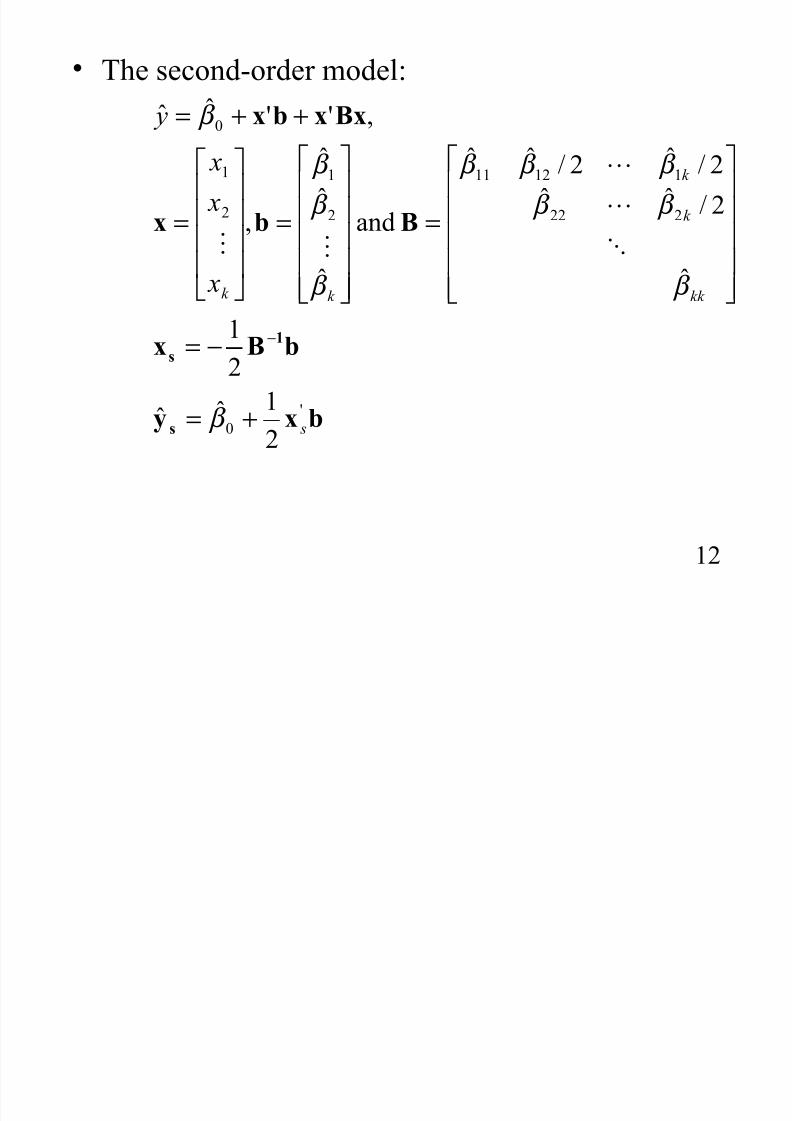
12
-he second/order model)
bxy
bBx
Bbx
Bxxbx
s
1
s
F0
222
11211
2
1
2
1
0
21::
2
1
:
29::
29:29::
and
:
:
:
*
*FF::
s
kk
k
k
k k x
x
x
y
+=
−=
=
=
=
++=
−
β
β
β β
β β β
β
β
β
β

7/25/2019 cahpter XI cyril
http://slidepdf.com/reader/full/cahpter-xi-cyril 13/19
1+
Characterizing the response surface)
= Contour plot or Canonical analysis
= Canonical form !see 'igure 11.B"
= Minimum response) i are all positi%e
= Ma(imum response) i are all negati%e
= Saddle point) i ha%e different signs
22
11::
k k s ww y y λ λ +++=
7/25/2019 cahpter XI cyril
http://slidepdf.com/reader/full/cahpter-xi-cyril 14/19
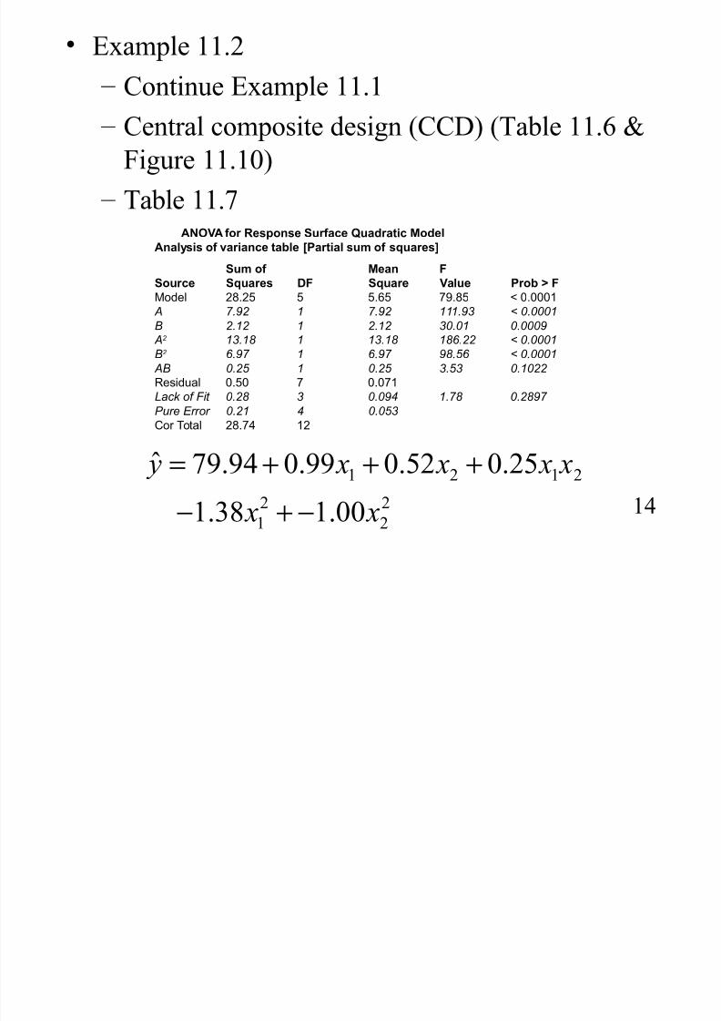
1
<(ample 11.2
= Continue <(ample 11.1
= Central composite design !CCE" !-a$le 11.7 ,'igure 11.10"
= -a$le 11.; ANOVA for Response Surface Quadratic Model
Analysis of variance table [Partial sum of squares]Sum of Mean
Source Squares ! Square Value Prob "
)odel 2(#2' ' '#$' 7"#(' * &#&&&1
A 7.92 1 7.92 111.93 < 0.0001
B 2.12 1 2.12 30.01 0.0009
A2 13.18 1 13.18 186.22 < 0.0001
B2 6.97 1 6.97 98.56 < 0.0001
AB 0.25 1 0.25 3.53 0.1022
Residual &#'& 7 &#&71
Lack of Fit 0.28 3 0.094 1.78 0.2897
Pure Error 0.21 4 0.053
Cor Total 2(#7% 12
1 2 1 2
2 21 2
: ;B.B 0.BB 0.52 0.25
1.+ 1.00
y x x x x
x x
= + + +
− + −

7/25/2019 cahpter XI cyril
http://slidepdf.com/reader/full/cahpter-xi-cyril 15/19
15
-he contour plot is gi%enin the natural %aria$les
!see 'igure 11.11"
-he optimum is at a$out
; minutes and 1;7.5
degrees
yield
A : ti m e
B
: t
e
m
p
(&#&& (2#'& ('#&& (7#'& "&#&&
17&#&&
172#'&
17'#&&
177#'&
1(&#&&
7 $ # " ' %
7 7 # $ & ' $
7 ( # 2 ' 7 !
7 ( # 2 ' 7 !
7 ( # " & ( "
7 " # ' $ & $
'

7/25/2019 cahpter XI cyril
http://slidepdf.com/reader/full/cahpter-xi-cyril 16/19
17
-he relationship $et#een ( and #)
= M is an orthogonal matri( and the columns of
M are the normalized eigen%ectors of 8.
Multiple response)
= -ypically* #e #ant to simultaneously optimizeall responses* or find a set of conditions #here
certain product properties are achie%ed
= O%erlay the contour plots !'igure 11.17"
= Constrained optimization pro$lem
"!F sxxMw −=
7/25/2019 cahpter XI cyril
http://slidepdf.com/reader/full/cahpter-xi-cyril 17/19
1;
11. <(perimental Eesigns for
'itting Response Surfaces Eesigns for fitting the first/order model
= -he orthogonal first/order designs
= G6G is a diagonal matri(
= 2 factorial and fractions of the 2 series in
#hich main effects are not aliased #ith each
others = 8esides factorial designs* include se%eral
o$ser%ations at the center.
= Simple( design

7/25/2019 cahpter XI cyril
http://slidepdf.com/reader/full/cahpter-xi-cyril 18/19
1
Eesigns for fitting the second/order model
= Central composite design !CCE"
= n' runs on 2 a(ial or star points* and nC centerruns
= Seuential e(perimentation
= -#o parameters) nC and α
= -he %ariance of the predicted response at ()
= Rotata$le design) -he %ariance of predicted
response is constant on spheres
= -he purpose of RSM is optimization and the
location of the optimum is unno#n prior to
running the e(periment.
xX)(X'x'x 1−= 2""!:! σ yVar

7/25/2019 cahpter XI cyril
http://slidepdf.com/reader/full/cahpter-xi-cyril 19/19
1B
3 !n'"19 yields a rotata$le central composite
design
= -he spherical CCE) Set 3 !"192
= Center runs in the CCE* nC) + to 5 center runs
= -he 8o(/8ehnen design) three/le%el designs
!see -a$le 11."
= Cu$oidal region)
face/centered central composite design !or
face/centered cu$e" 3 1
nC32 or +