Illinois State Water Survey Division SURFACE WATER SECTION

SWS Contract Report 485

CACHE RIVER BASIN: HYDROLOGY, HYDRAULICS,

AND SEDIMENT TRANSPORT

VOLUME 2: MATHEMATICAL MODELING

by Misganaw Demissie, Ta Wei Soong, and Rodolfo Camacho

Prepared for the Illinois Department of Conservation

Champaign, Illinois January 1990

CACHE RIVER BASIN: HYDROLOGY, HYDRAULICS, AND SEDIMENT TRANSPORT

VOLUME 2: MATHEMATICAL MODELING

by Misganaw Demissie, Ta Wei Soong, and Rodolfo Camacho

Illinois State Water Survey 2204 Griffith Drive

Champaign, IL 61820-7495

Prepared for the Illinois Department of Conservation

Champaign, Illinois January 1990

CONTENTS

Page

Introduction 1 Rationale for Application of Models in the Cache River Basin 1 Report Organization 3 Acknowledgments 3

Lower Cache River Modeling 5 HEC-1 Model 5

Model Assumptions and Structure 5 Precipitation 6 Abstractions 6 Runoff 8

Unit Hydrograph Method 8 Kinematic Wave Method 11

Calibration Methodology 16 Application of HEC-1 in the Lower Cache River Basin 17

Methodology 17 Lower Cache River Subbasins 19 Input Data Parameters and Selection of Methods 19

Precipitation 19 Abstractions 22 Runoff 22 Geometry 22 Resistance Coefficients 22

Calibration 23 Storms for Calibration 23 Calibration Results 25 Verification 25

Model Application for Routing of Flows in the LCRNA 26 Storage Relationships within the LCRNA . 26 Water Balance and Parameter Transferability Verification 27 Flow Routing in the LCRNA 28

Upper Cache River Modeling 45 HEC-6 Model 45

Input Data Requirements 46 Potential Uses and Limitations 47

Application of the HEC-6 Model in the Upper Cache River 48 Geometric Data 48 Sediment Data 52

Bed Material Gradation 52 Inflow Sediment Load 52

Sediment Load in the Main-Stem Stream 56 Sediment Inflow from Tributary Streams 60

Hydrologic Data 62 Operating Rules and Downstream Boundary Conditions 63

Calibration of the HEC-6 Model for the Upper Cache River 67

Concluded on next page

HEC-6 Results for the Upper Cache River 69 Flood Elevations 69 Sediment Transport 74

Summary 98

References 100

Appendix: Geometry of Cross Sections That Were Used in the HEC-6 Model for the Upper Cache River printed in a separate volume

CACHE RIVER BASIN: HYDROLOGY, HYDRAULICS, AND SEDIMENT TRANSPORT VOLUME 2: MATHEMATICAL MODELING

by Misganaw Demissie, Ta Wei Soong, and Rodolfo Camacho

INTRODUCTION

Rationale for Application of Models in the Cache River Basin Mathematical models are useful tools for investigating future conditions under various

assumed scenarios. Data collection alone does not provide sufficient information to explain previous or future conditions. The length of time and the variability of the conditions under which data are collected are usually limited and do not cover all possible conditions. However, field data are needed for calibrating model parameters used in mathematical equations that represent the physical laws controlling water and sediment movement in a drainage basin. They also provide input data to mathematical models, as well as valuable information for selecting, modifying, and developing these models.

It is imperative to use mathematical models when contemplating implementation of management alternatives. Such models provide the capability of simulating expected conditions resulting from assumed measures, and thus they provide the basis for selecting among alternative measures. Along with a well-designed data collection program, mathematical models provide excellent management tools for watersheds and river basins.

Mathematical models were used to compute runoff from storm events, flood elevations, and the transport of sediment in the Cache River basin. These aspects of hydrology, hydraulics, and sediment transport of the basin are the primary problems that have to be managed properly to accommodate the various uses of the river. Models were applied for two separate areas shown in figure 1. The first area is the segment of the Lower Cache River that drains into the Lower Cache River Natural Area (LCRNA). The major problem investigated in this segment of the river was flood elevations. The second area is the Post Creek Cutoff - Upper Cache River segment from the junction with the Ohio River, to the Route 146 bridge upstream of the Little Black Slough wetland area. The primary problem in this area is the entrenchment of the Upper Cache River channel and its impacts on the hydrology of wetlands, especially the area around Heron Pond and Little Black Slough.

After several hydrologic models were evaluated, the U.S. Army Corps of Engineers' (USACOE) HEC-1 model (1987) was selected for modeling the rainfall-runoff processes in the Lower Cache River segment. HEC-1 was selected because of the extensive use of this model in

1

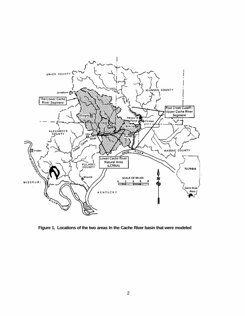
Figure 1. Locations of the two areas In the Cache River basin that were modeled

2

the United States. Since its original release in 1968, it has been tested extensively in many watersheds in the United States with satisfactory results. Furthermore, HEC-l's calibration capabilities and optimization techniques of runoff hydrographs are appropriate for the hydrologic modeling of the Lower Cache River because of the types of data that are available. Using this program permits proper simulation of water movement in the watershed and of storage changes in the Lower Cache River Natural Area.

For modeling sediment transport and surface water profiles in the Upper Cache River, the HEC-6 model (USACOE, 1977) was selected on the basis of its capabilities and the nature of the problems in the Cache River. The experience of Illinois State Water Survey (ISWS) researchers in applying the HEC-6 model to investigate various hydraulic problems in Illinois, and the satisfactory nature of the results from the model, also played an important role in its selection (Demissie et al., 1986, 1988; Demissie and Stephanatos, 1985). Other models of similar capabilities were compared to the HEC-6, and their results were found to be no better. Moreover, they require more data and computer time.

This report presents the results of the applications of the HEC-1 model to the Lower Cache River and of the HEC-6 model to the Upper Cache River. Brief discussions of the models, their data requirements, and the types of results they generate are also included.

Report Organization This report is one of two volumes prepared as the completion report for the Cache River

basin project. In addition to these two volumes, a report has been prepared that outlines problems, alternative solutions, and recommendations. This volume deals only with the application and results of the mathematical models used in the project. It has two major sections: "Lower Cache River Modeling" and "Upper Cache River Modeling." As mentioned previously, two different models were used: the HEC-1 model for the Lower Cache River and the HEC-6 model for the Upper Cache River. The two major sections discuss these models, as well as their important assumptions, input data requirements, calibration procedures, and limitations. They then discuss the applications of the models to the two segments of the Cache River, including the input data for the different conditions considered, the calibration results, and finally the results of the models. The appendix to the report is printed in a separate volume along with the appendices to volume 1.

Acknowledgments This work was accomplished as part of the regular work of the Illinois State Water

Survey (ISWS) under the administrative guidance of Richard G. Semonin, Chief; Richard J.

3

Schicht, former Assistant Chief; Michael L. Terstriep, Head of the Surface Water Section; and Nani G. Bhowmik, Assistant Head of the Surface Water Section.

The work upon which this report is based was supported in part by funds provided by the Illinois Department of Conservation (IDOC). Marvin Hubbell is the project manager for IDOC and provided valuable guidance for the project. Renjie Xia, graduate student in civil engineering at the University of Illinois, assisted in the modeling effort. Richard Allgire and Laura Keefer, who are responsible for data collection and analysis for the Cache River project, provided all the necessary data for calibration and verification of the models. Paul Makowski, formerly of ISWS, assisted in the collection and analysis of bed and bank material. Becky Howard typed the report, Gail Taylor edited it, and Linda Riggin prepared the illustrations.

4

LOWER CACHE RIVER MODELING

Modeling for the Lower Cache River consisted primarily of simulating watershed runoff from the tributary streams that drain into the Lower Cache River Natural Area (LCRNA) and then routing the flows through the swamp to determine flood elevations for varying conditions. The model was further used in evaluating the hydrologic impacts of alternative management scenarios for the LCRNA

The model selected for investigating runoff and flood conditions in the Lower Cache River is the HEC-1 model of the USACOE, which is widely used in the United States and many other countries. A brief discussion of the model and its capabilities, and results of the application of the model, are presented in the following sections. More detailed information on HEC-1 is provided by the USACOE (1987) in the HEC-1 Flood Hydrograph Package-User's Manual.

HEC-1 Model The first version of the HEC-1 model, released in October 1968, was designed by the

Hydrologic Engineering Center (HEC) to simulate the surface water runoff from a watershed that is generated by precipitation. The main outputs of the HEC-1 model are runoff hydrographs for given watersheds under various precipitation and antecedent conditions. The model has gone through major revisions and expansions since 1968. The present version of the program (1987) is a major revision of the 1973 revision of the original. Dam-break (HEC-1DB), project optimization (HEC-1GS), and kinematic wave (HEC-1KW) special versions have been incorporated in the program. A personal computer (PC) version, developed in 1984, includes all the capabilities of the main-frame version except for the flood damage and ogee spillway options, which were omitted because of memory and compiler limitations. Only the hydrograph simulation portion of the program was used for the hydrologic modeling of the Lower Cache.

Model Assumptions and Structure The HEC-1 model represents a basin by means of hydrologically interconnected units or

subareas. Hydrologic processes in each unit are assumed to be uniform, and model parameters are averages for these subareas. Besides the assumption of spatial averages, temporal averages are also assumed for the selected computational time interval. The time interval chosen should be small enough for adequate model application. The model can simulate only single storm events since consideration is not given to soil moisture changes in periods without rainfall.

The river basin to be modeled is divided into hydrologically interconnected subbasins based on topographic maps. This subdivision is based on the assumption of uniform average hydrologic conditions for each subbasin, as well as on particular interests in studying

5

predetermined areas. The model provides different options for computing the runoff hydrograph for each subbasin through its different components for overland flow and river and reservoir routing.

The rainfall-runoff modeling in HEC-1 is performed by using mathematical relationships for the different hydrologic processes schematically represented in figure 2. These processes include precipitation, abstractions (losses, such as those due to infiltration), runoff, and base flow. The HEC-1 Flood Hydrograph Package allows the user to choose among different methodologies to simulate most of these processes. Brief descriptions of the methods used to simulate some of these processes are presented below.

Precipitation. Precipitation values must be provided as input data to the model. Precipitation is assumed to be uniform over the subbasin area and is represented in HEC-1 by rainfall depths over a specified time interval conforming to the rainfall hyetograph. Precipitation may be provided as a basin average or a weighted precipitation average at gages. In the first case, the total precipitation and its temporal variation are provided for the whole basin. In the second case, the total storm precipitation for a subbasin is obtained from weighted average measurements at different gages. Therefore the hyetograph computed for a subbasin from different gages is obtained by the following formula:

where PRCP (i) is the subbasin-average precipitation for the ith time interval, PRCPR (i, j) is the precipitation at the recording station j for the ith time interval, WTR (j) is the weight assigned to the station, and N is the number of gages.

The program also provides the options of generating the standard project storm, SPS; probable maximum precipitation, PMP; and synthetic storms from depth duration data. These options are frequently used for planning and design based on long-term studies of precipitation data for the region under consideration.

Abstractions. The precipitation that does not contribute to runoff is defined as abstractions or losses. These losses may be due to interception, depression storage, or infiltration.

HEC-1 provides four different methods for computing precipitation loss: 1) the initial and uniform loss rate; 2) the exponential loss rate; 3) the SCS curve number; and 4) the Holtan loss

6

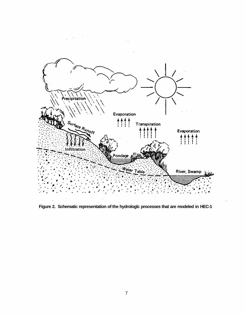
Figure 2. Schematic representation of the hydrologlc processes that are modeled in HEC-1

7

rate. The HEC-1 does not consider soil moisture or surface storage recovery, limiting the applicability of the model to single storm events.

In the initial and uniform loss rate method, all the initial precipitation is considered lost until the initial loss specified as input is matched. From that point on, the losses by infiltration are assumed to be constant.

The exponential loss rate method empirically represents the loss rate of precipitation by an exponential function. This function takes into account the antecedent soil moisture and the infiltration capacity according to the characteristics of the soil in the basin. Estimates of the different parameters of this function can be obtained by using the optimization routines of HEC-1.

The Soil Conservation Service method (SCS curve number) provides relationships for the precipitation loss between the initial surface moisture storage, curve number, and total runoff depth of the event under consideration. The curve number is a function of the soil type, land use, and antecedent soil moisture condition, and is obtained from tables developed by the SCS.

In the Holtan loss rate method (Holtan et al., 1975), the loss f is computed on the basis of a power function for the infiltration capacity plus a constant factor as shown in equation 2.

f = G I * a * S A B E + FC (2)

In this equation the constant FC represents the steady-state infiltration rate, which is determined from the soil type; GI is the growth index of the crop expressed as a percentage of maturity; a is the infiltration capacity available in storage; SA is the available storage in the soil surface; and BE is an empirical exponent commonly taken as 1.4.

Runoff. Runoff from the effective rainfall (total rainfall minus losses) may be computed by either the unit hydrograph method or the kinematic wave approach. The different options available in HEC-1 are discussed briefly in the following sections.

Unit Hydrograph Method. The unit hydrograph was first proposed by Sherman (1932) and was defined as "the hydrograph of direct runoff resulting from 1 inch of effective rainfall generated uniformly over the basin area at a uniform rate during a specified period of time or duration." The concept is illustrated in figure 3, where the flow hydrograph generated by 1 inch of effective rainfall is shown. The main advantage of using the unit hydrograph is that it reflects the physical characteristics of the subbasin and is assumed not to be storm-dependent. Therefore direct runoff from multiple storms can be linearly superimposed. The best results from using the unit hydrograph theory are achieved if the hydrologic conditions selected for the analysis represent the assumptions behind this theory as closely as possible (Sherman, 1932). In

8

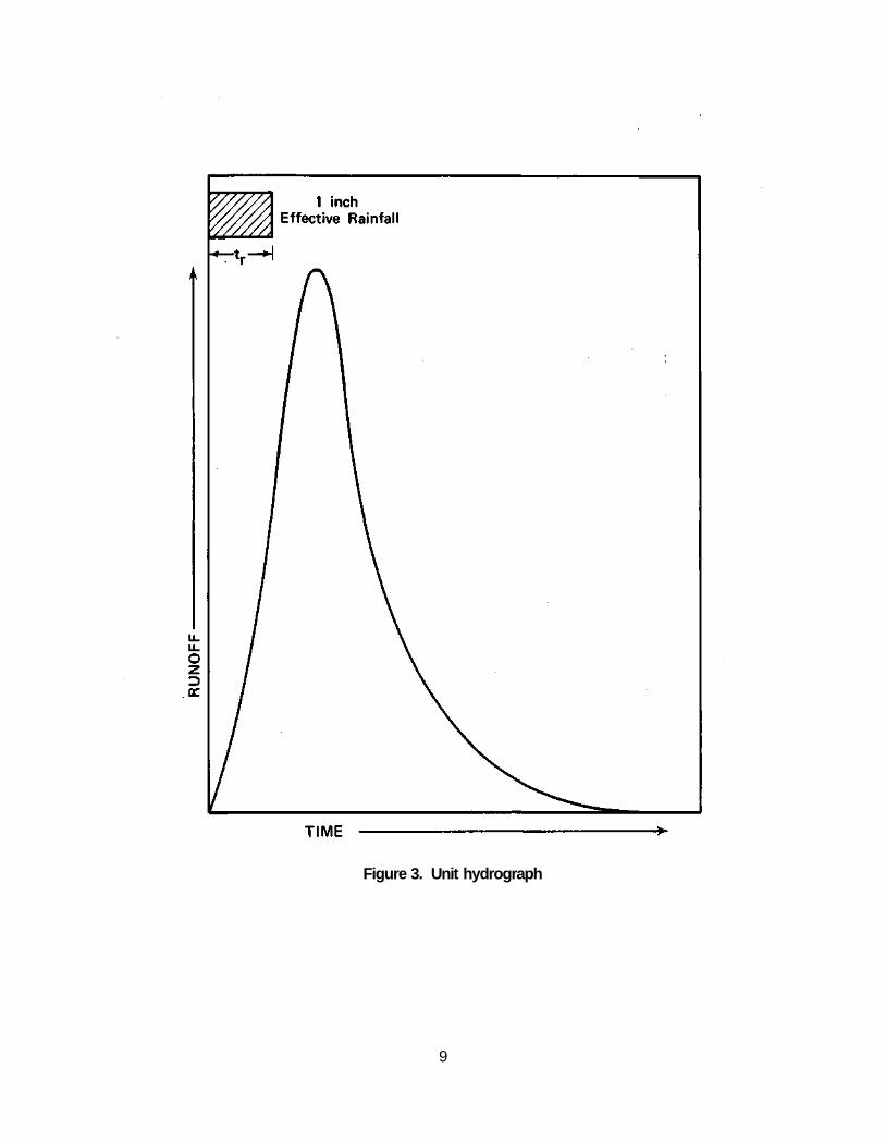
Figure 3. Unit hydrograph

9

other words, as pointed out by Chow (1964), first, the effective rainfall is uniformly distributed over the subbasin and falls within its specified time interval; second, the base time duration of direct runoff is constant for an effective unit rainfall; and finally, the direct runoff ordinates of a common base time duration are proportional to the total amount of runoff. On the basis of these assumptions, selection of short-duration storms is recommended because they are produced by high-intensity rainfalls that are uniform over the duration of the storm. Moreover, the drainage areas should not be very large to avoid nonuniform distribution of rainfall within the area under consideration.

Once a unit hydrograph is obtained for a particular duration for the subbasin, the effective rainfall is transformed to the direct runoff by using the equation:

where Q(i) is the subbasin outflow at the end of period i, U(j) is the jth ordinate of the unit hydrograph, and X(i) is the average rainfall excess for the ith period. This equation states that the runoff discharge Q(i) is the accumulation of different periods of effective rainfall.

The HEC-1 model offers methods for determining three different synthetic unit hydrographs: the Clark unit hydrograph, Snyder unit hydrograph, and SCS dimensionless unit hydrograph.

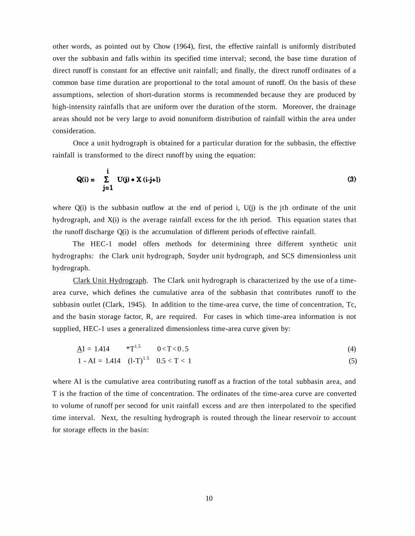
Clark Unit Hydrograph. The Clark unit hydrograph is characterized by the use of a time-area curve, which defines the cumulative area of the subbasin that contributes runoff to the subbasin outlet (Clark, 1945). In addition to the time-area curve, the time of concentration, Tc, and the basin storage factor, R, are required. For cases in which time-area information is not supplied, HEC-1 uses a generalized dimensionless time-area curve given by:

AI = 1.414 *T1.5 0<T<0 .5 (4) 1 - AI = 1.414 (l-T)1.5 0.5 < T < 1 (5)

where AI is the cumulative area contributing runoff as a fraction of the total subbasin area, and T is the fraction of the time of concentration. The ordinates of the time-area curve are converted to volume of runoff per second for unit rainfall excess and are then interpolated to the specified time interval. Next, the resulting hydrograph is routed through the linear reservoir to account for storage effects in the basin:

10

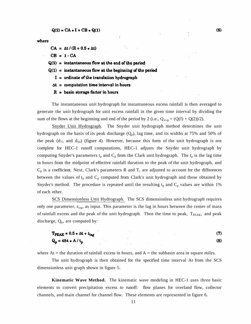
The instantaneous unit hydrograph for instantaneous excess rainfall is then averaged to generate the unit hydrograph for unit excess rainfall in the given time interval by dividing the sum of the flows at the beginning and end of the period by 2 (i.e., Qavg = (Q(l) + Q(2))/2).

Snyder Unit Hydrograph. The Snyder unit hydrograph method determines the unit hydrograph on the basis of its peak discharge (Qp), lag time, and its widths at 75% and 50% of the peak (d75 and d50) (figure 4). However, because this form of the unit hydrograph is not complete for HEC-1 runoff computations, HEC-1 adjusts the Snyder unit hydrograph by computing Snyder's parameters tp and Cp from the Clark unit hydrograph. The tp is the lag time in hours from the midpoint of effective rainfall duration to the peak of the unit hydrograph, and Cp is a coefficient. Next, Clark's parameters R and Tc are adjusted to account for the differences between the values of tp and Cp computed from Clark's unit hydrograph and those obtained by Snyder's method. The procedure is repeated until the resulting tp and Cp values are within 1% of each other.

SCS Dimensionless Unit Hydrograph. The SCS dimensionless unit hydrograph requires only one parameter, tlag, as input. This parameter is the lag in hours between the center of mass of rainfall excess and the peak of the unit hydrograph. Then the time to peak, TPEAK, and peak discharge, Qp, are computed by:

where At = the duration of rainfall excess in hours, and A = the subbasin area in square miles. The unit hydrograph is then obtained for the specified time interval At from the SCS

dimensionless unit graph shown in figure 5.

Kinematic Wave Method. The kinematic wave modeling in HEC-1 uses three basic elements to convert precipitation excess to runoff: flow planes for overland flow, collector channels, and main channel for channel flow. These elements are represented in figure 6.

11

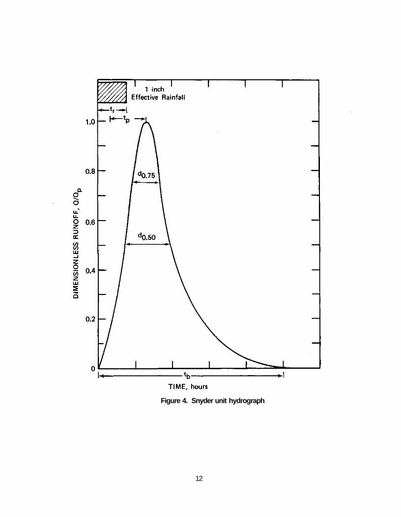
Figure 4. Snyder unit hydrograph

12

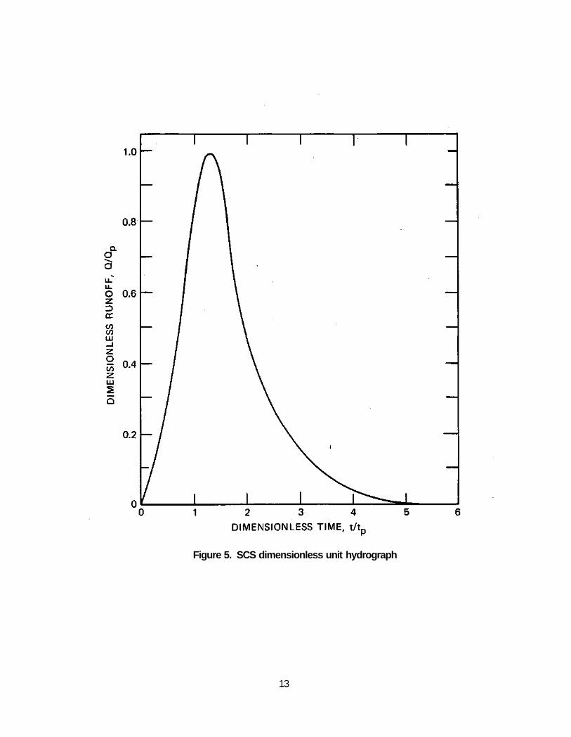
Figure 5. SCS dimensionless unit hydrograph

13

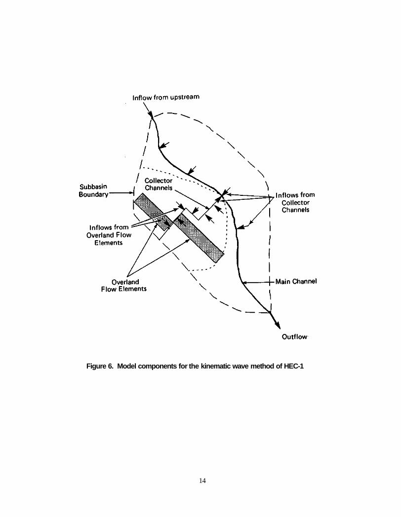
Figure 6. Model components for the kinematic wave method of HEC-1

14

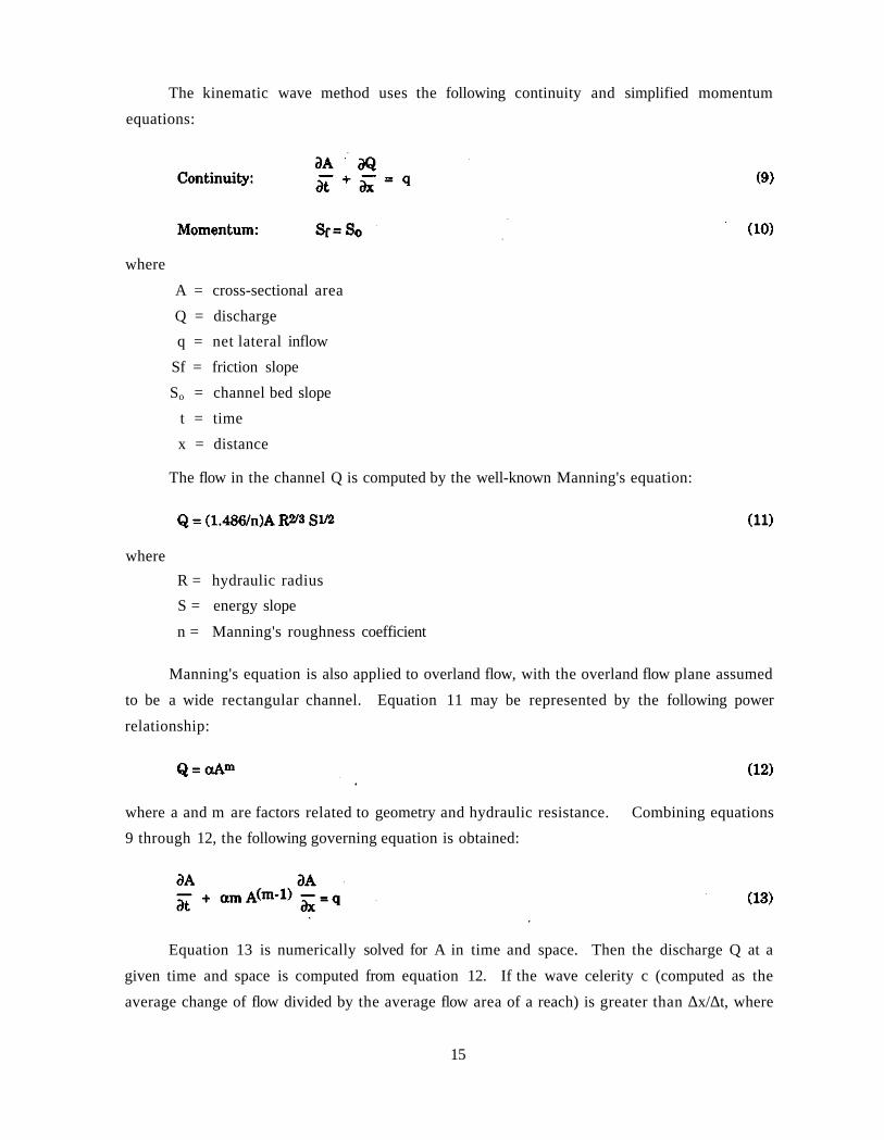
The kinematic wave method uses the following continuity and simplified momentum equations:

where A = cross-sectional area Q = discharge q = net lateral inflow

Sf = friction slope So = channel bed slope

t = time x = distance

The flow in the channel Q is computed by the well-known Manning's equation:

where R = hydraulic radius S = energy slope n = Manning's roughness coefficient

Manning's equation is also applied to overland flow, with the overland flow plane assumed to be a wide rectangular channel. Equation 11 may be represented by the following power relationship:

where a and m are factors related to geometry and hydraulic resistance. Combining equations 9 through 12, the following governing equation is obtained:

Equation 13 is numerically solved for A in time and space. Then the discharge Q at a given time and space is computed from equation 12. If the wave celerity c (computed as the average change of flow divided by the average flow area of a reach) is greater than Δx/Δt, where

15

Ax and At are the computational space and time intervals respectively, equation 9 should be

solved numerically instead of equation 13 to guarantee numerical stability.

Calibration Methodology The application of mathematical models of rainfall-runoff processes generally requires

model calibration for the watershed under consideration. The calibrations are based on rainfall data measured in the watershed and on runoff measured at its outlet. The results of the calibration determine the parameters for the different equations for future runoff predictions and for simulating runoff from hypothetical storms.

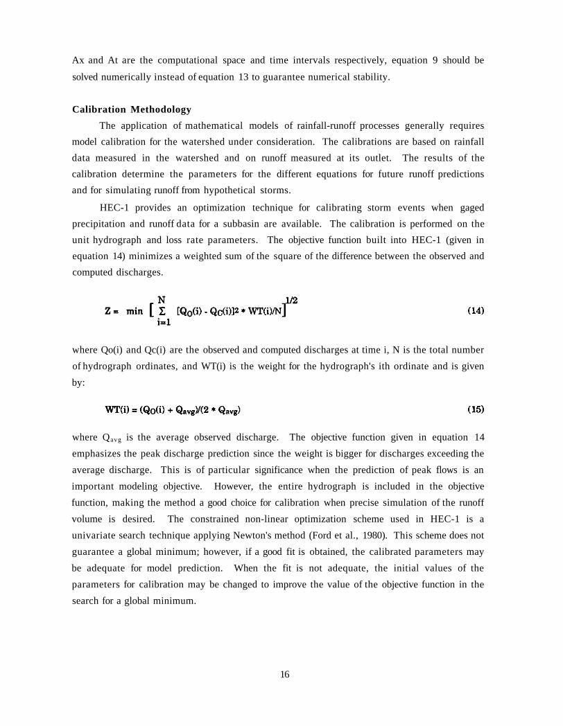
HEC-1 provides an optimization technique for calibrating storm events when gaged precipitation and runoff data for a subbasin are available. The calibration is performed on the unit hydrograph and loss rate parameters. The objective function built into HEC-1 (given in equation 14) minimizes a weighted sum of the square of the difference between the observed and computed discharges.

where Qo(i) and Qc(i) are the observed and computed discharges at time i, N is the total number of hydrograph ordinates, and WT(i) is the weight for the hydrograph's ith ordinate and is given by:

where Qavg is the average observed discharge. The objective function given in equation 14 emphasizes the peak discharge prediction since the weight is bigger for discharges exceeding the average discharge. This is of particular significance when the prediction of peak flows is an important modeling objective. However, the entire hydrograph is included in the objective function, making the method a good choice for calibration when precise simulation of the runoff volume is desired. The constrained non-linear optimization scheme used in HEC-1 is a univariate search technique applying Newton's method (Ford et al., 1980). This scheme does not guarantee a global minimum; however, if a good fit is obtained, the calibrated parameters may be adequate for model prediction. When the fit is not adequate, the initial values of the parameters for calibration may be changed to improve the value of the objective function in the search for a global minimum.

16

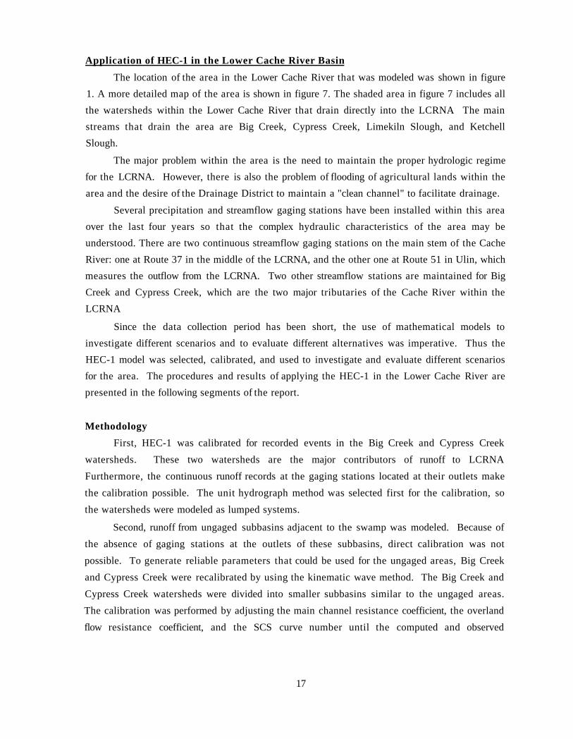
Application of HEC-1 in the Lower Cache River Basin The location of the area in the Lower Cache River that was modeled was shown in figure

1. A more detailed map of the area is shown in figure 7. The shaded area in figure 7 includes all the watersheds within the Lower Cache River that drain directly into the LCRNA The main streams that drain the area are Big Creek, Cypress Creek, Limekiln Slough, and Ketchell Slough.

The major problem within the area is the need to maintain the proper hydrologic regime for the LCRNA. However, there is also the problem of flooding of agricultural lands within the area and the desire of the Drainage District to maintain a "clean channel" to facilitate drainage.

Several precipitation and streamflow gaging stations have been installed within this area over the last four years so that the complex hydraulic characteristics of the area may be understood. There are two continuous streamflow gaging stations on the main stem of the Cache River: one at Route 37 in the middle of the LCRNA, and the other one at Route 51 in Ulin, which measures the outflow from the LCRNA. Two other streamflow stations are maintained for Big Creek and Cypress Creek, which are the two major tributaries of the Cache River within the LCRNA

Since the data collection period has been short, the use of mathematical models to investigate different scenarios and to evaluate different alternatives was imperative. Thus the HEC-1 model was selected, calibrated, and used to investigate and evaluate different scenarios for the area. The procedures and results of applying the HEC-1 in the Lower Cache River are presented in the following segments of the report.

Methodology First, HEC-1 was calibrated for recorded events in the Big Creek and Cypress Creek

watersheds. These two watersheds are the major contributors of runoff to LCRNA Furthermore, the continuous runoff records at the gaging stations located at their outlets make the calibration possible. The unit hydrograph method was selected first for the calibration, so the watersheds were modeled as lumped systems.

Second, runoff from ungaged subbasins adjacent to the swamp was modeled. Because of the absence of gaging stations at the outlets of these subbasins, direct calibration was not possible. To generate reliable parameters that could be used for the ungaged areas, Big Creek and Cypress Creek were recalibrated by using the kinematic wave method. The Big Creek and Cypress Creek watersheds were divided into smaller subbasins similar to the ungaged areas. The calibration was performed by adjusting the main channel resistance coefficient, the overland flow resistance coefficient, and the SCS curve number until the computed and observed

17

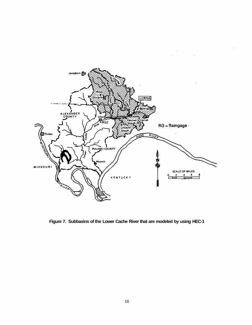
Figure 7. Subbasins of the Lower Cache River that are modeled by using HEC-1

18

hydrographs matched. Resistance coefficients and runoff curve numbers determined for Big Creek and Cypress Creek were then extrapolated to ungaged subbasins according to their similarities.

Finally, the HEC-1 model was run for the whole area. Since no calibration was possible for the ungaged subbasins, and to verify the kinematic wave parameters extrapolated from Big Creek and Cypress Creek, some overall calibration or adjustment of the kinematic wave parameters for ungaged subbasins was needed. This was accomplished by comparing measured and computed shapes and volumes of hydrographs of the whole area for the calibration events. The shape of the resulting hydrograph after being routed through the swamp was compared with that recorded for the Cache River at Route 51 or at Route 37 where stages are recorded. The volume of the resulting hydrograph was verified by a water balance in the LCRNA area, with consideration given to the measured outflow and change of storage within the LCRNA. Once these adjustments were made, the calibrated model could be used for modeling hypothetical future storms in the Lower Cache River basin.

Lower Cache River Subbasins For modeling purposes by the kinematic wave method, the area of the Lower Cache River

draining into the LCRNA was subdivided into 36 small subbasins on the basis of 7-1/2 minute USGS topographic maps. The size and number of subbasins were selected on the basis of uniformity of hydrologic conditions within each subbasin. Figure 8 schematically shows these subbasins and their drainage patterns towards the swamp. The areas of these subbasins range from 0.73 to 10.9 square miles, with an average of 4.2 square miles. For the HEC-1 model, these subbasins are hydrologically linked as depicted schematically in figure 8. The important physical properties of all the subbasins, including those within the Big Creek and Cypress Creek watersheds, are summarized in table 1.

Input Data Parameters and Selection of Methods For modeling and calibrating the Lower Cache River, the following input data methods

were used.

Precipitation. Precipitation information was obtained from rainfall records at each of the three raingages within the area being modeled (figure 7). The distribution of rainfall or the hyetograph was provided to the model as average rainfall depths over a predetermined time interval. These hyetographs were obtained at each raingage in the study area. In addition to the hyetographs, the corresponding spatial weight (in percentage) of each gage was provided.

19

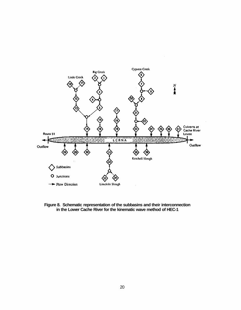
Figure 8. Schematic representation of the subbasins and their interconnection in the Lower Cache River for the kinematic wave method of HEC-1

20

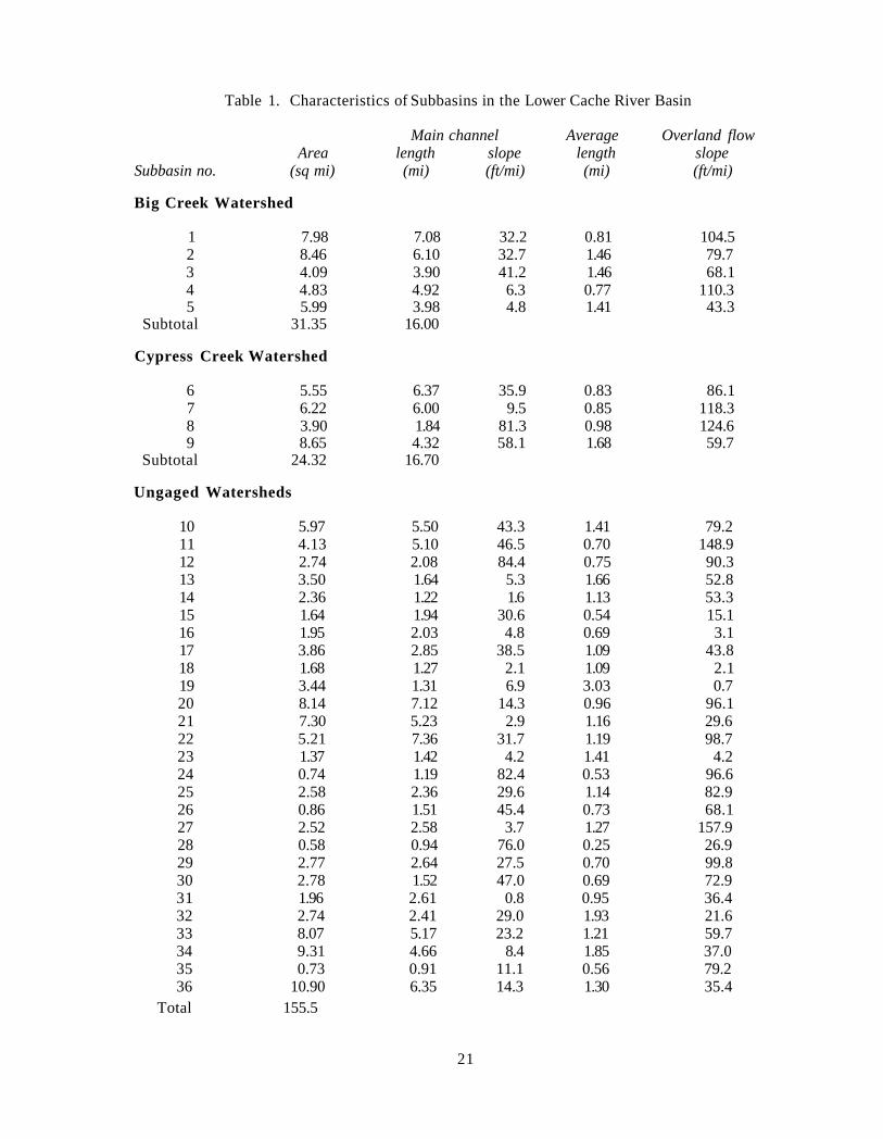
Table 1. Characteristics of Subbasins in the Lower Cache River Basin

Main channel Average Overland flow Area length slope length slope

Subbasin no. (sq mi) (mi) (ft/mi) (mi) (ft/mi)

Big Creek Watershed

1 7.98 7.08 32.2 0.81 104.5 2 8.46 6.10 32.7 1.46 79.7 3 4.09 3.90 41.2 1.46 68.1 4 4.83 4.92 6.3 0.77 110.3 5 5.99 3.98 4.8 1.41 43.3

Subtotal 31.35 16.00

Cypress Creek Watershed

6 5.55 6.37 35.9 0.83 86.1 7 6.22 6.00 9.5 0.85 118.3 8 3.90 1.84 81.3 0.98 124.6 9 8.65 4.32 58.1 1.68 59.7

Subtotal 24.32 16.70

Ungaged Watersheds

10 5.97 5.50 43.3 1.41 79.2 11 4.13 5.10 46.5 0.70 148.9 12 2.74 2.08 84.4 0.75 90.3 13 3.50 1.64 5.3 1.66 52.8 14 2.36 1.22 1.6 1.13 53.3 15 1.64 1.94 30.6 0.54 15.1 16 1.95 2.03 4.8 0.69 3.1 17 3.86 2.85 38.5 1.09 43.8 18 1.68 1.27 2.1 1.09 2.1 19 3.44 1.31 6.9 3.03 0.7 20 8.14 7.12 14.3 0.96 96.1 21 7.30 5.23 2.9 1.16 29.6 22 5.21 7.36 31.7 1.19 98.7 23 1.37 1.42 4.2 1.41 4.2 24 0.74 1.19 82.4 0.53 96.6 25 2.58 2.36 29.6 1.14 82.9 26 0.86 1.51 45.4 0.73 68.1 27 2.52 2.58 3.7 1.27 157.9 28 0.58 0.94 76.0 0.25 26.9 29 2.77 2.64 27.5 0.70 99.8 30 2.78 1.52 47.0 0.69 72.9 31 1.96 2.61 0.8 0.95 36.4 32 2.74 2.41 29.0 1.93 21.6 33 8.07 5.17 23.2 1.21 59.7 34 9.31 4.66 8.4 1.85 37.0 35 0.73 0.91 11.1 0.56 79.2 36 10.90 6.35 14.3 1.30 35.4

Total 155.5

21

Abstractions. The initial loss and uniform continuous loss rate method and the SCS curve number were used to account for abstractions in HEC-1. The initial loss and uniform continuous loss rate method was selected because of its simplicity. Moreover, as pointed out by Ford et al. (1980), an initial loss and uniform loss rate is more appropriate when temporal and spatial distribution of rainfall may not be well defined. In addition to the initial loss and uniform continuous loss rate method, SCS curve number values were used for comparison since these values are well documented in the literature and are also used in the kinematic wave approach.

Runoff. Direct runoff hydrographs must be available and specified to the program for model calibration. Complete runoff hydrographs were obtained from the continuous stage records at the gaging stations within the area being modeled by using their rating curves. The runoff ordinates from the observed hydrographs were provided with the same time interval as that used for the hyetograph.

For simulating hypothetical storms, unit hydrograph approaches and the kinematic wave method were used. Unit hydrograph parameters or other runoff and abstraction parameters, obtained through the calibration process, were given as input parameters.

For the unit hydrograph approach, Clark's method was selected for calibration of the Big Creek and Cypress Creek watersheds. As reported by Ford et al. (1980), a detailed time-area curve is not required since the dimensionless time-area curve provided by the model gives satisfactory results. This was also verified by Melching (1987). The Snyder and SCS unit hydrographs were also tested for comparison purposes.

Geometry. For the unit hydrograph, as well as for the kinematic wave approach, the subbasin areas are required by the model. These areas were obtained from digitized topographic maps. In addition to the area of each subbasin, the kinematic wave approach requires the average lengths and slopes of the overland flow subcatchments. The main channel length and slope, and its typical cross-sectional shape, are also required. Average overland flow lengths and slopes were obtained from topographic maps, and channel cross-sectional shapes were obtained from field surveys.

Resistance Coefficients. Overland flow and channel resistance coefficients are required input parameters of the kinematic wave approach. These values were initially determined by field observations and tables of Manning's resistance coefficient (Chow, 1959). The overland flow resistance coefficients were obtained from tables given by Crawford and Linsley (1966) and Woolhiser (1975).

22

Calibration Calibration of the Big Creek and Cypress Creek watersheds was performed first because

of the availability of gaged precipitation and runoff data for them. As pointed out before, these subbasins are the major contributors of water to the Lower Cache River and the LCRNA. Three different approaches to the runoff calibration were analyzed: the Clark unit hydrograph; the SCS dimensionless unit hydrograph; and the Snyder unit hydrograph. For the abstractions due to infiltration and interception, the initial loss and uniform continuous loss rate and SCS curve number were calibrated. HEC-1 has a built-in optimization technique for calibration using the three approaches.

Runoff from ungaged subbasins was modeled by using the kinematic wave approach. HEC-1 does not have a built-in routine for automatic calibration of the kinematic wave parameters. Therefore the continuous loss rate or curve number parameters obtained by the automatic calibration are fixed in the kinematic wave approach. Then the overland and channel flow resistance coefficients are modified until the computed runoff hydrograph matches the measured hydrograph at the subbasin outlet.

Storms for Calibration. Storm events from Water Years 1986 and 1987 were selected for calibration purposes. The selection of these events was based on the following criteria:

1) The events had to be single storms of considerable magnitude with no appreciable spatial variation of precipitation within the watershed.

2) For the events selected, complete rainfall and runoff records had to be available at the gaging stations.

3) The direct runoff from the events had to be the consequence of precipitation excess, with no snowmelt.

4) Enough events had to be chosen during the year that seasonal variation of the parameters could be identified by the calibration.

On the basis of these criteria, six storms were selected for the calibration of the Big Creek and Cypress Creek watersheds. The times of occurrence and the main characteristics of these events are summarized in table 2.

Calibration of these events is performed on the basis of the direct runoff hydrographs. Therefore, to obtain the direct runoff hydrograph, base flow from the recorded runoff hydrograph is separated by the following procedure: The events for calibration are isolated events and therefore the base flow may be considered constant for the rising limb of the hydrograph. In the recession limb, the slope of the direct runoff hydrograph becomes constant. Then a line with the same slope may be drawn backwards up to the inflection point of the recession limb, signaling

23

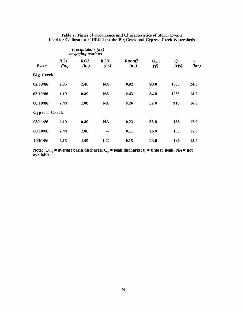
Table 2. Times of Occurrence and Characteristics of Storm Events Used for Calibration of HEC-1 for the Big Creek and Cypress Creek Watersheds

Precipitation (in.) at gaging stations

RG1 RG2 RG3 Runoff Qaug Qp tp Event (in.) (in.) (in.) (in.) (cfs) (cfs) (hrs)

Big Creek

02/03/86 2.35 2.40 NA 0.92 90.0 1605 24.0

03/12/86 1.19 0.89 NA 0.43 84.0 1085 18.0

08/10/86 2.44 2.88 NA 0.26 52.0 918 16.0

Cypress Creek

03/11/86 1.19 0.89 NA 0.23 35.0 136 12.0

08/10/86 2.44 2.88 -- 0.11 16.0 178 15.0

12/01/86 1.16 1.05 1.22 0.15 23.0 140 18.0

Note: Qavg = average basin discharge; Qp = peak discharge; tp = time to peak; NA = not available.

24

the base flow at the end of the event. Next, the base flow at the peak and the inflection point are connected by a straight line. This methodology is illustrated in figure 9 for the measured runoff at Big Creek for the event of March 12,1986.

Calibration Results. Calibration of the Big Creek and Cypress Creek watersheds was performed by following the procedure outlined in the previous section. The resulting parameters from the calibration are given in table 3. Initial and continuous water losses are higher for the summer event than for the winter and spring events, as shown in table 3, because of higher interception and infiltration rates during the summer. The presence of vegetation retards the runoff rate, allowing the water more time to penetrate the soil. This is also reflected by the runoff curve numbers, which are smaller for the summer event. The calibrated parameters for Big Creek are more consistent than those for Cypress Creek.

Table 4 shows the percent error in the runoff volume, peak discharge (Qp), and time to peak (tp) for the events calibrated by using the Clark unit hydrograph and the initial loss continuous water loss method. The coefficient of model fit efficiency, EFF (in percent), is also shown in the table. This coefficient, proposed by Nash and Sutcliffe (1971), indicates the efficiency of the calibration. EFF is computed by the following equation:

where Qo(i) is the observed discharge at time i, Qavg is the average observed discharge, Qc(i) is the computed discharge for time i, and N is the number of time periods.

In general the calibration results are acceptable. The efficiency factors are particularly high for Big Creek, and runoff volume and time-to-peak percentage errors are very small. The calibration results are better for Big Creek than for Cypress Creek.

Figures 10 through 15 show comparisons of the observed hydrographs for Big Creek and Cypress Creek and those computed by using the Clark unit hydrograph and initial loss and continuous water loss model, for the calibration events summarized in table 2.

Verification. To test the accuracy of the calibration, the storm of February 28, 1987, was used as a verification storm. Runoff from the storm was simulated by using the parameters obtained for the calibration events. This storm had recorded precipitation of 2.13 inches at raingage 2 and 2.19 inches at gage 3 in a period of 48 hours. The maximum observed peak

25

discharge at the gaging station on Big Creek was 1023 cfs, with a total runoff of 1.1 inches. At the Cypress Creek gaging station, the recorded peak discharge was 390 cfs, with a total runoff of 0.93 inches.

The results of this verification in terms of percent error in the total volume, peak discharge, and time to peak and the efficiency factor, EFF, defined by equation 16, are as follows:

Percent error EFF Volume Qp tp (%)

Big Creek 15.0 2.1 0.0 71.2

Cypress Creek 9.5 16.1 -4 90.1

The overall verification results are better for Cypress Creek than for Big Creek, as indicated by the efficiency factor EFF. However, the peak discharge for Cypress Creek is overestimated by 16.1% as compared to only 2.1% for Big Creek. The observed and computed hydrographs for the verification storm are compared in figures 16 and 17 for Big Creek and Cypress Creek, respectively.

Model Application for Routing of Flows in the LCRNA Storage Relationships within the LCRNA

Because of the importance of water storage in the floodplain, relations between storage volume and elevation are required for different portions of the area to properly simulate the water-surface elevations and movements of water in the LCRNA. On the basis of 10-foot contour topographic maps of the Lower Cache River drainage basin, surface areas at contour elevations of 330, 340, and 350 feet msl (above mean sea level) were determined for the following four segments along the Cache River in the LCRNA: Route 51 to Cache Chapel Road; Cache Chapel Road to Perks Road; Perks Road to Route 37; and Route 37 to the culverts at the Cache River levee (sometimes referred to as the Forman Floodway levee). The relative locations and sizes of these four segments are shown in figure 18. Curves for elevation versus storage volume were then developed for each segment by using the conic method for computing reservoir volumes as illustrated in figure 19 (USACOE, 1987).

Figures 20 through 23 show the curves for elevation versus storage volume for each of the segments mentioned above, and figure 24 shows the relation for the whole Lower Cache River valley between Route 51 and the culverts at the Cache River levee.

26

Water Balance and Parameter Transferability Verification To further verify the calibration of the HEC-1 and the transferability of parameters to

ungaged subbasins in the Lower Cache River basin, a water balance check was performed in the LCRNA for selected events for which precipitation and runoff were measured. This was accomplished by considering the following fundamental storage relationship, which relates the change in storage, Δs/Δt, to the difference between inflow, I, and outflow, O:

In equation 17, I represents all inputs of water to the LCRNA for a period of time At. These inputs are the modeled runoffs from all the subbasins of the Lower Cache River that drain into the LCRNA, and the direct rainfall over the area. O is the outflow of water from the LCRNA at its outlets at Route 51 and the culverts at the Cache River levee during the same period of time At. Other secondary losses such as evaporation and losses to ground water at the swamp can be included in the 0 term. AS is the change of storage within the LCRNA for the period At.

Two events (one in winter and one in summer), during which stages along the LCRNA were recorded at different times, were selected. Rainfall amounts at the three gaging stations and the peak flows at the Route 51 gage during these events were as follows:

Precipitation in inches at gaging stations peak flow

Event RG1 RG2 RG3 at Route 51 (cfs)

02/28/87 - 2.13 2.19 668 06730/87 1.88 3.42 1.81 563

Figures 25 and 26 show the water surface elevations along the LCRNA at the beginning and end of the events.

Inputs of water from all subbasins draining into the LCRNA were computed by HEC-1. Outflows of water from the LCRNA were determined from discharge measurements at Route 51 and estimated discharges of the culverts. The time interval At was taken as 50 hours, and water surface elevations were recorded at the beginning and end of this period (figures 25 and 26). The corresponding changes in storage were determined by using the stage-versus-volume curves developed for the different sections along the LCRNA.

The only unmeasured variable in equation 17 is I, and it was determined by using the HEC-1 model. Equation 17 was applied for the events of February 28 and June 30, 1987, with

27

the curve number or loss factor in the HEC-1 model adjusted until the equality of the equation was achieved. This resulted in curve numbers of 90 for the February event and 72 for the June event. These curve numbers are in agreement with the values obtained after calibration, as shown in table 3.

Figures 27 and 28 show the input hydrographs, which are the computed hydrographs for Big Creek, Cypress Creek, and Limekiln Slough, and the outflow hydrographs at Route 51 and the culverts for the events of February 28 and June 30, respectively. In figures 27 and 28, the inflow hydrograph peaks are significantly greater than the outflow hydrograph peaks. This peak flow attenuation is due to the storage capacity of the LCRNA, which stores most of the inflow from tributary streams during flood events and releases it slowly.

Flow Routing in the LCRNA HEC-1 flow routing options were used for routing flood hydrographs through the

LCRNA. The event of June 30, 1987, was chosen for testing the flow routing technique. The selected flow routing technique was verified by comparisons of observed and model-predicted stages at different locations in the LCRNA.

The flow directions in the swamp for the event of June 30 are shown in figure 26. Field observations during this event showed that all inflow into the LCRNA east of Perks Road was flowing towards the culverts. Inflow west of Perks Road was observed to flow towards Route 51. However, it should be pointed out that the observed flow directions for the event of June 30 may not necessarily occur during other events. The flow directions depend on the areal rainfall distribution and initial surface water elevations in the LCRNA. In general, it is found that as events progress in time, and water elevations in the LCRNA rise, the slope of the water surface between Route 37 and the Cache River levee decreases. Eventually, the water surface level between Route 37 and the levee becomes horizontal, and thereafter water flowing into the LCRNA east of Perks Road may flow westward towards Route 51. These flow direction changes were observed at Route 37 and other locations in the LCRNA for several events. At the beginning of major events, in the rising limb of the hydrograph, the flow direction in the Cache River east of the junction with Big Creek is generally to the east. After the peak, in the receding part of the hydrograph, water flows either west or east depending upon the water surface slope between Route 37 and the levee. The water surface slope and therefore the flow direction in the LCRNA are mainly controlled by the outlet capacities on both ends of the LCRNA.

In general, three flow behaviors are found in the LCRNA during a storm event, and therefore three modeling approaches are followed for initial conditions similar to those of the event of June 30, 1987 (figure 26):

28

1) At the beginning of the event, water entering into the swamp west of Perks Road flows towards Route 51, while water entering the LCRNA east of Perks Road flows towards the culverts. Therefore a channel flow routing technique is used for routing between Perks Road and Route 51 and between Route 37 and the culverts at the levee. From Perks Road to Route 37, a level pool storage routing is used.

2) After the water surface between Route 37 and the levee becomes horizontal and water starts to flow west throughout the LCRNA, a level pool storage routing of all inflows between the levee and Cache Chapel Road is used.

3) Finally, if the event is extremely large and the outlet at Route 51 is not able to pass all the incoming flow, more water will be backed up in the LCRNA. The surface water slope between Cache Chapel Road and Route 51 will approach horizontal. Then all inflow hydrographs into the swamp are routed by using a level pool routing technique with outflow at Route 51 and the culverts at the levee. The outflow through the culverts depends on the water level at the levee and is computed by using a rating curve developed for the culverts. The outflow at Route 51 is computed by using the rating curve for the gaging station.

The routing of hydrographs between Perks Road and Cache Chapel Road and between Perks Road and Route 37 was performed by using the modified Puls method (Chow, 1964). A storage-versus-outflow relationship is provided as input to the model. This relationship is obtained from the storage-elevation curve between Perks and Cache Chapel Roads (figure 21) and a rating curve at Cache Chapel Road. For channel routing from Cache Chapel Road to Route 51 and from Route 37 to the culverts, the kinematic wave approach was selected from among the different techniques provided in the HEC-1 model.

Figures 29 and 30 show the observed and computed stages at Route 37 and Route 51 for the event of June 30, 1987. Although further refinement of the routing procedure is needed, the agreement between the observed and computed stages is generally good, and the model can be used for preliminary evaluations of different scenarios and alternatives.

29

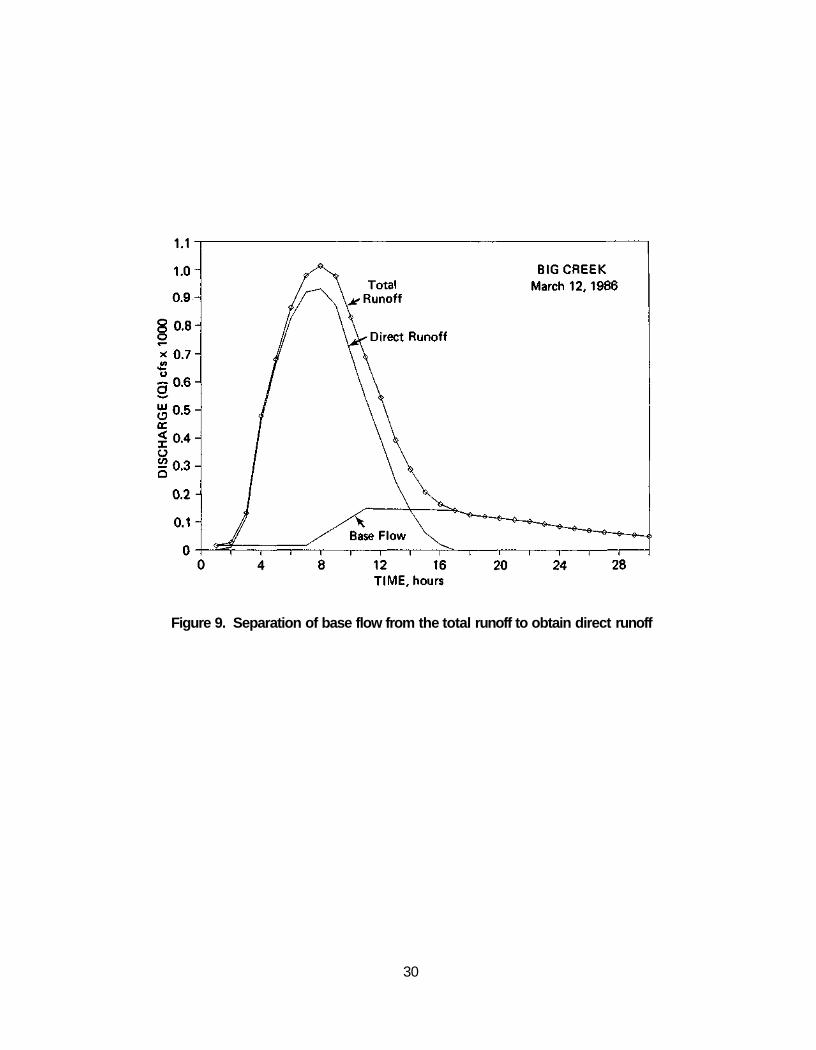
Figure 9. Separation of base flow from the total runoff to obtain direct runoff

30

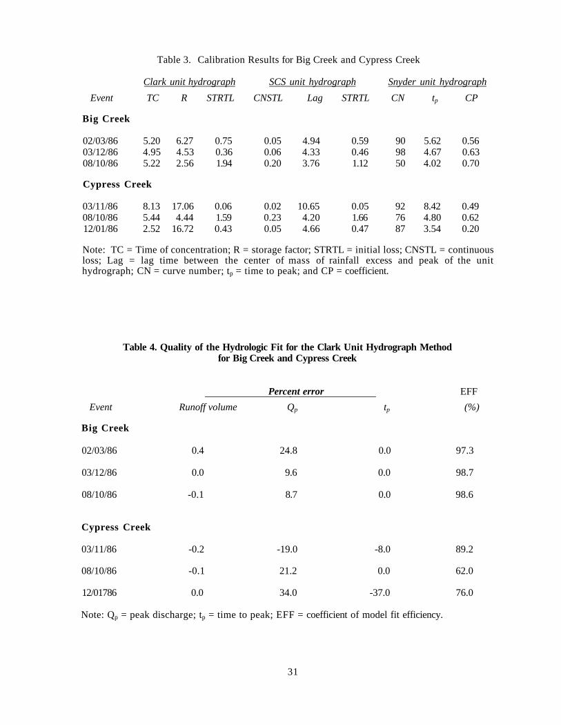
Table 3. Calibration Results for Big Creek and Cypress Creek

Clark unit hydrograph SCS unit hydrograph Snyder unit hydrograph Event TC R STRTL CNSTL Lag STRTL CN tp CP

Big Creek

02/03/86 5.20 6.27 0.75 0.05 4.94 0.59 90 5.62 0.56 03/12/86 4.95 4.53 0.36 0.06 4.33 0.46 98 4.67 0.63 08/10/86 5.22 2.56 1.94 0.20 3.76 1.12 50 4.02 0.70

Cypress Creek

03/11/86 8.13 17.06 0.06 0.02 10.65 0.05 92 8.42 0.49 08/10/86 5.44 4.44 1.59 0.23 4.20 1.66 76 4.80 0.62 12/01/86 2.52 16.72 0.43 0.05 4.66 0.47 87 3.54 0.20

Note: TC = Time of concentration; R = storage factor; STRTL = initial loss; CNSTL = continuous loss; Lag = lag time between the center of mass of rainfall excess and peak of the unit hydrograph; CN = curve number; tp = time to peak; and CP = coefficient.

Table 4. Quality of the Hydrologic Fit for the Clark Unit Hydrograph Method for Big Creek and Cypress Creek

Percent error EFF Event Runoff volume Qp tp (%)

Big Creek

02/03/86 0.4 24.8 0.0 97.3

03/12/86 0.0 9.6 0.0 98.7

08/10/86 -0.1 8.7 0.0 98.6

Cypress Creek

03/11/86 -0.2 -19.0 -8.0 89.2

08/10/86 -0.1 21.2 0.0 62.0

12/01786 0.0 34.0 -37.0 76.0

Note: Qp = peak discharge; tp = time to peak; EFF = coefficient of model fit efficiency.

31

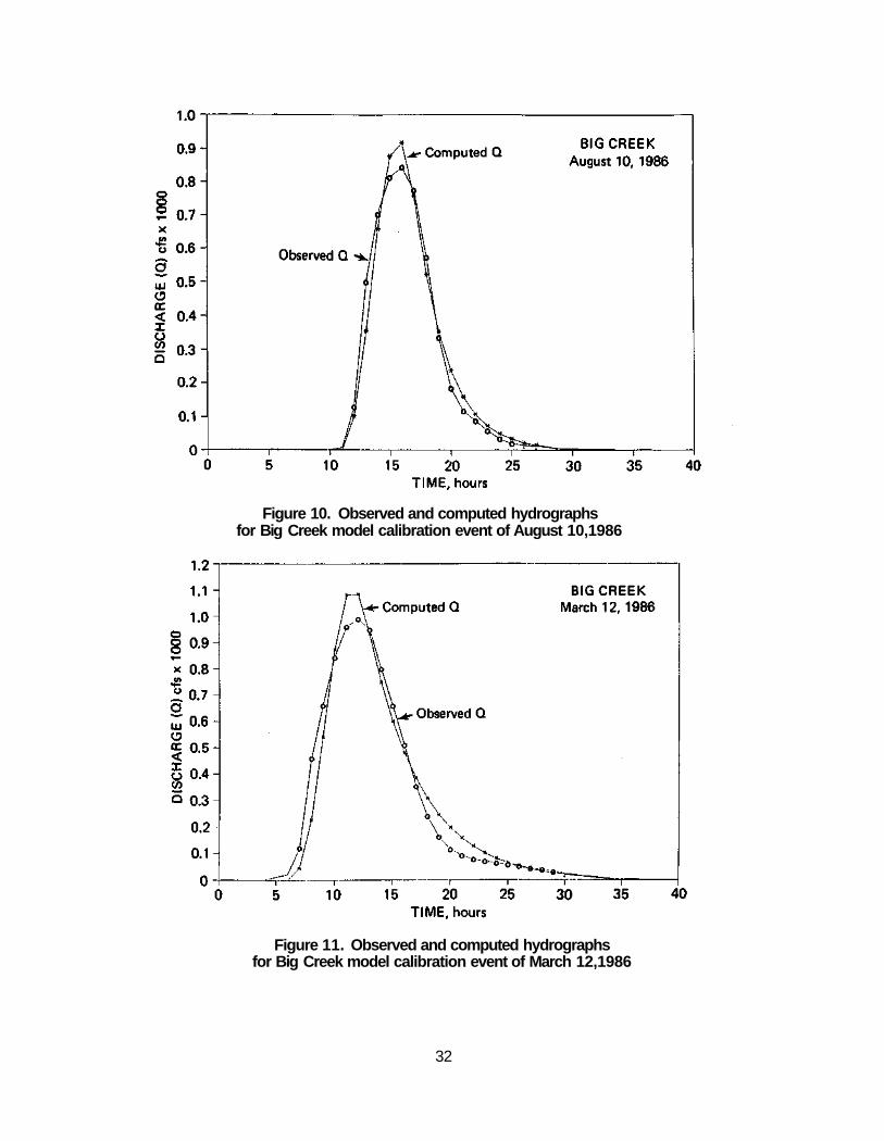
Figure 11. Observed and computed hydrographs for Big Creek model calibration event of March 12,1986

32

Figure 10. Observed and computed hydrographs for Big Creek model calibration event of August 10,1986

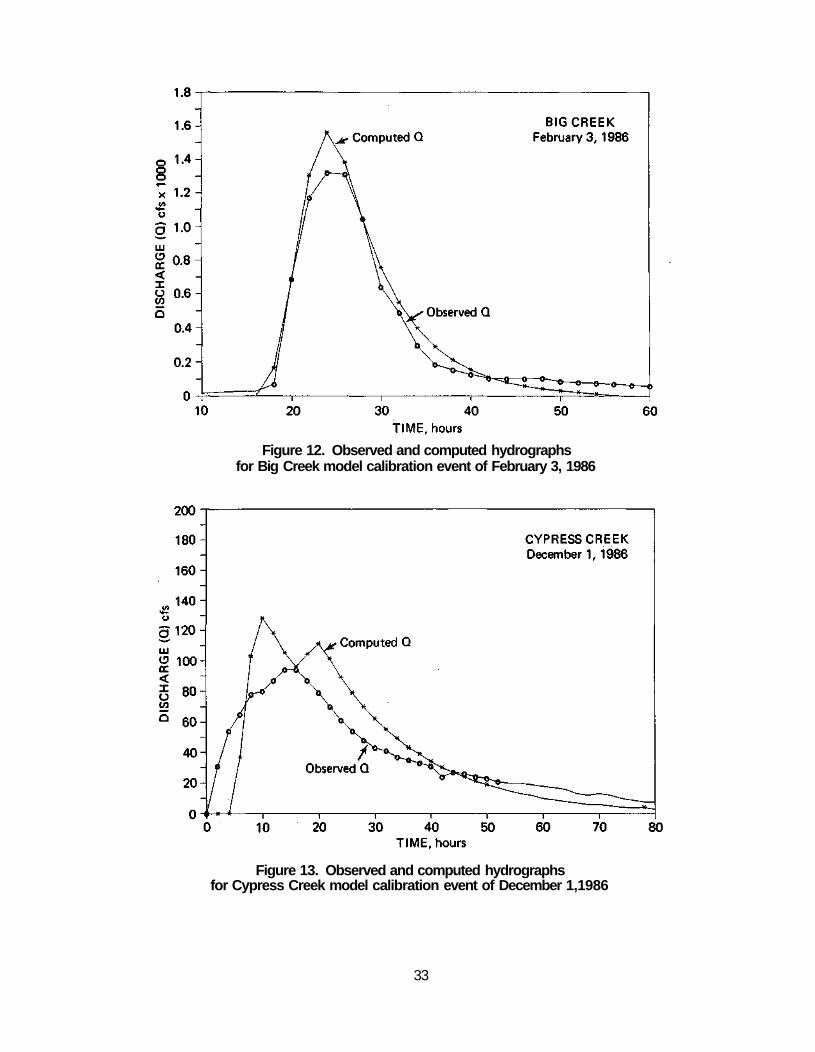
Figure 13. Observed and computed hydrographs for Cypress Creek model calibration event of December 1,1986

33

Figure 12. Observed and computed hydrographs for Big Creek model calibration event of February 3, 1986

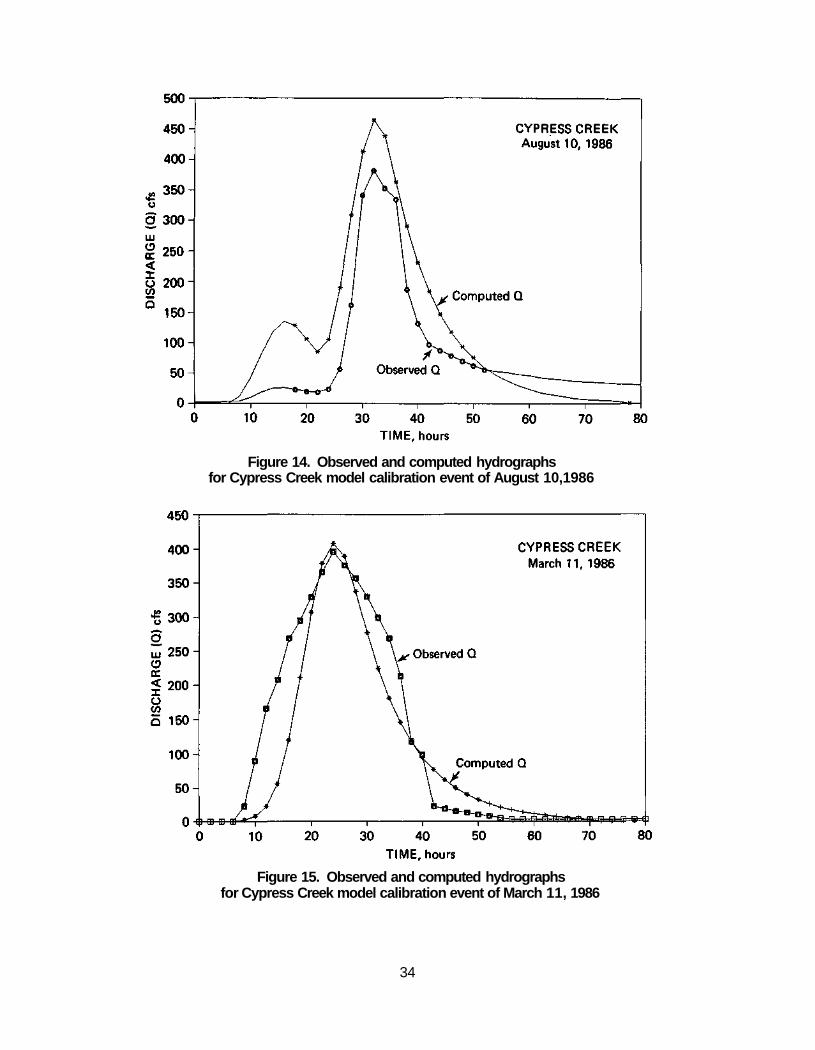
Figure 15. Observed and computed hydrographs for Cypress Creek model calibration event of March 11, 1986

34

Figure 14. Observed and computed hydrographs for Cypress Creek model calibration event of August 10,1986

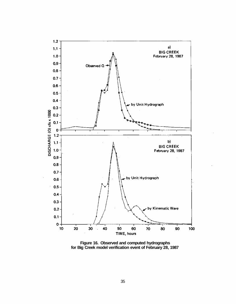
Figure 16. Observed and computed hydrographs for Big Creek model verification event of February 28, 1987

35

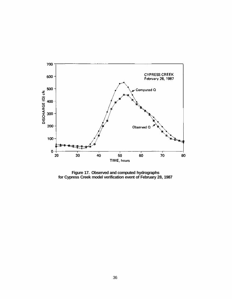
Figure 17. Observed and computed hydrographs for Cypress Creek model verification event of February 28, 1987

36

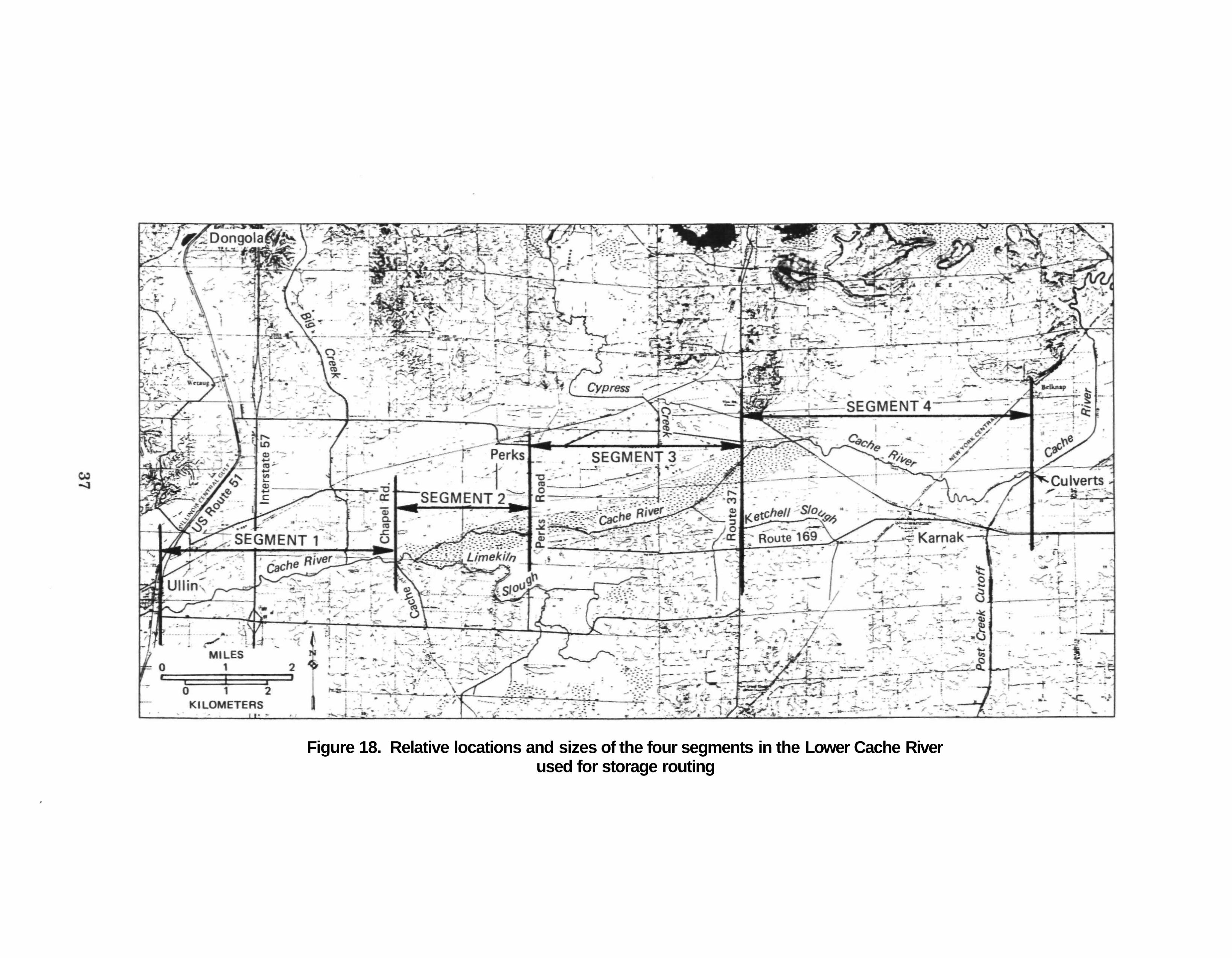
Figure 18. Relative locations and sizes of the four segments in the Lower Cache River used for storage routing

*

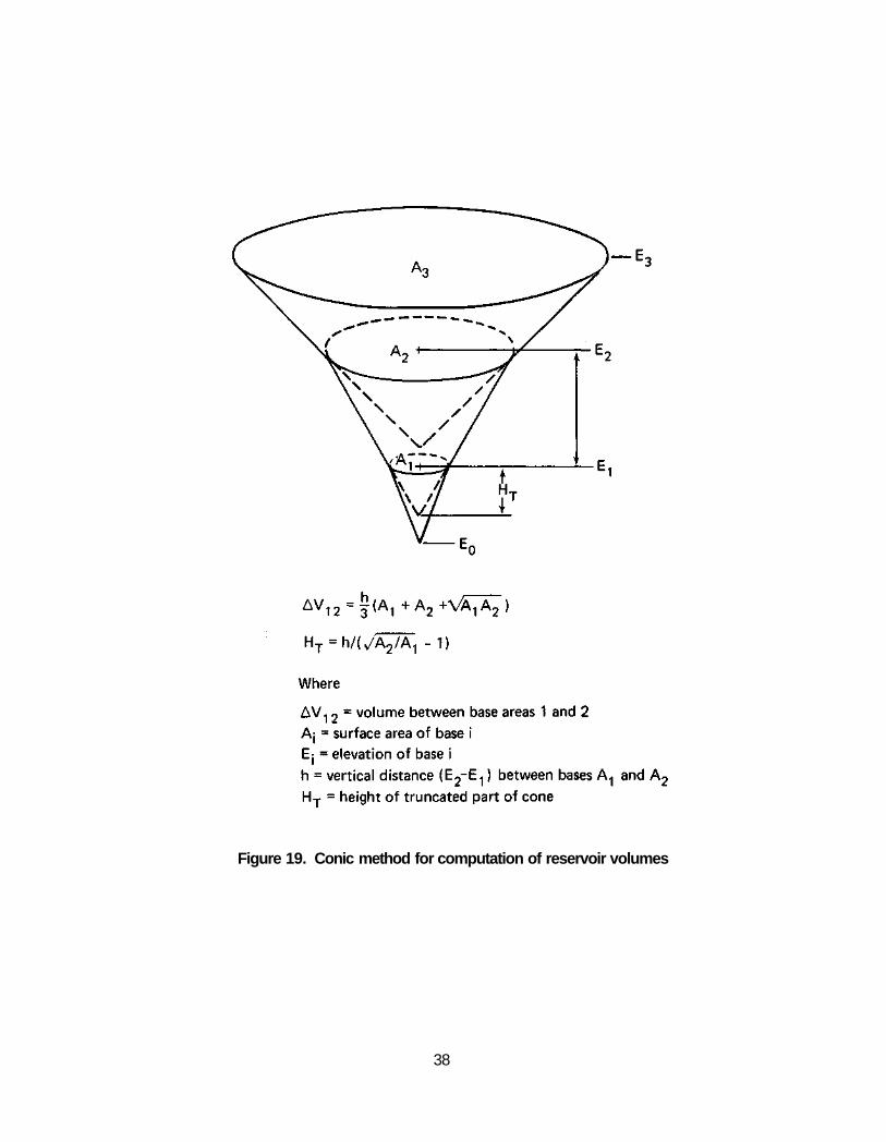
Figure 19. Conic method for computation of reservoir volumes

38

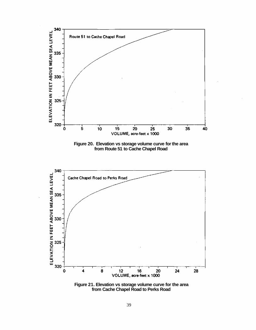
Figure 20. Elevation vs storage volume curve for the area from Route 51 to Cache Chapel Road

Figure 21. Elevation vs storage volume curve for the area from Cache Chapel Road to Perks Road

39

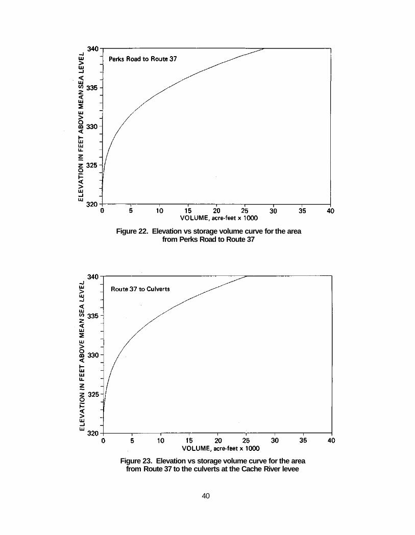
Figure 22. Elevation vs storage volume curve for the area from Perks Road to Route 37

Figure 23. Elevation vs storage volume curve for the area from Route 37 to the culverts at the Cache River levee

40

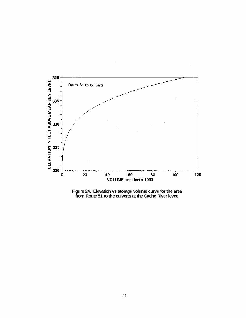
Figure 24. Elevation vs storage volume curve for the area from Route 51 to the culverts at the Cache River levee

41

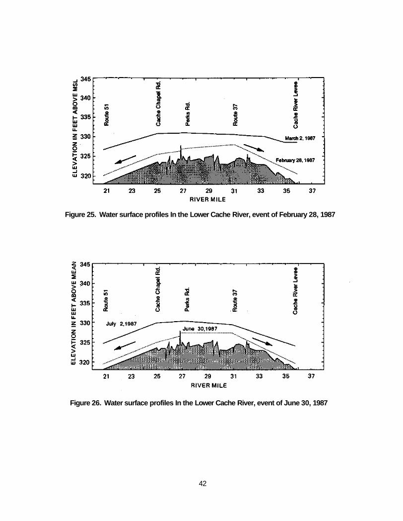
Figure 25. Water surface profiles In the Lower Cache River, event of February 28, 1987

Figure 26. Water surface profiles In the Lower Cache River, event of June 30, 1987

42

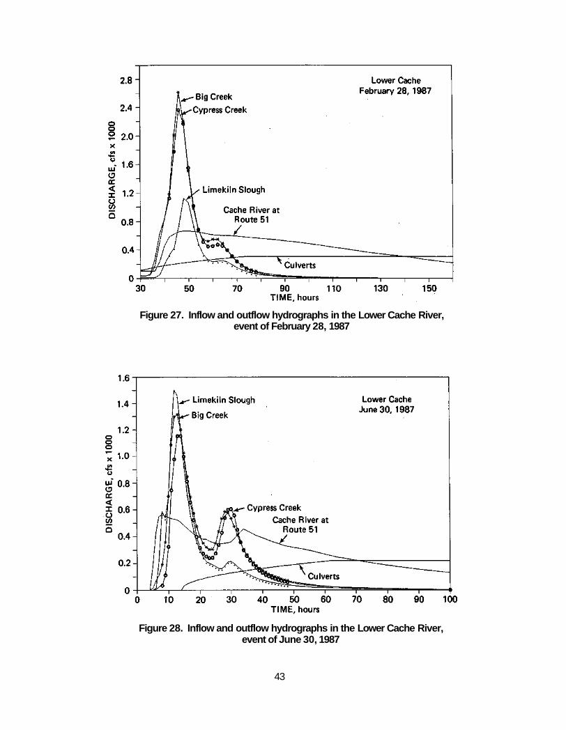
Figure 27. Inflow and outflow hydrographs in the Lower Cache River, event of February 28, 1987

Figure 28. Inflow and outflow hydrographs in the Lower Cache River, event of June 30, 1987

43

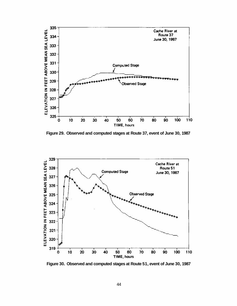
Figure 29. Observed and computed stages at Route 37, event of June 30, 1987

Figure 30. Observed and computed stages at Route 51, event of June 30, 1987

44

UPPER CACHE RIVER MODELING

The purpose of the modeling effort for the Upper Cache River is different from that for the Lower Cache River. In the Upper Cache River, the major concern is channel entrenchment and lateral gully formations; therefore modeling for the Upper Cache River was used to investigate sediment transport and channel scour. It was also used to evaluate the effectiveness of remedial measures that might be implemented in the Upper Cache River to retard or stop the entrenchment of the stream channels.

As mentioned in the introduction, the HEC-6 was selected as the best sediment transport model to use for the Upper Cache River. The following subsections of this report include discussions of the HEC-6 model and its application to the Upper Cache River. Initially the HEC-6 model is discussed in general terms, with brief discussions of the equations, computational procedures, input data requirements, and the potential uses and limitations of the model. Then the application of the model to the Upper Cache River is discussed. The report outlines all the geometric, sediment, and hydrologic data used in the model, discusses the calibration of the model for the Upper Cache River, and presents the results of the model.

HEC-6 Model The HEC-6 model is a one-dimensional flow model designed to analyze scour and

deposition of sediment in rivers and reservoirs. It simulates the ability of a stream to transport sediment and computes the scour and deposition of sand, silt, and clay in streams and reservoirs. Before any sediment transport computations are carried out, the HEC-6 performs the necessary hydraulic calculations, which include determination of water surface profiles and velocities. This is done in a manner similar to that in the water surface profile computations program of the HEC-2 (USACOE, 1982).

The basic equation used in the model is the equation for the continuity of sediment material given as:

where

B = width of deposit or scour area (movable bed) G = sediment load

ys = depth of sediment deposit or scour above a stable layer t = time x = distance along the channel

45

The HEC-6 model uses an implicit finite difference scheme to solve equation 18. The computational procedure in the model is as follows:

Step 1: The program computes the water surface profile and all the pertinent hydraulic parameters (elevation, slope, velocity, depth, and width) at each cross section along the study reach. The water surface profile is calculated by using the backward step method to solve the energy equation in the same way as in the HEC-2 water surface profile computations (USACOE, 1982).

Step 2: Using the hydraulic data obtained during the calculations of water surface profiles, the program calculates the inflowing sediment load, armoring, equilibrium depth, gradation of material in the active layer, transport capacity, etc., for each cross section. The transport capacity is determined from empirical relations incorporated in the model. The available options for such relations are: 1) Toffaleti's application of Einstein's bed load function (Toffaleti, 1966); 2) Laursen's relationship as modified by Madden for small rivers (Laursen, 1958; USACOE, 1977); 3) the DuBoys relationship (Vanoni, 1977); 4) Yang's streampower equation (Yang, 1976); or 5) any relationship developed by the user for a particular study. The relationship has to be specified in a form whereby the transport capacity per unit width is a function of the product of the water depth and the energy slope. For the forms of the different sediment transport equations and detailed discussions of them, the reader is referred to Vanoni (1977), Graf (1971), Garde and Raju (1985), and Simons and Senturk (1977).

Step 3: The program calculates the sediment load leaving the study reach and then changes the volume of bed material to reflect scour or deposition. The depth of deposit or scour is adjusted to reflect the new volume. The above procedure is repeated for a sequence of water discharges (derived from the discretized hydrograph) and the corresponding sediment loads. The changes are calculated with respect to time for each reach and with respect to distance along the stream for the different reaches within the study area.

Input Data Requirements The input data needed to run HEC-6 can be grouped into four categories, as described in

USACOE (1977):

1) Geometric data. Cross section coordinates, reach lengths, and Manning's n-values are required for water surface calculations. In addition, the movable bed portion of each cross section and the depth of sediment layers have to be inputted.

2) Sediment data. Inflow sediment load data, gradation of bed material in the streambed, and fluid and sediment properties are needed.

3) Hydrologic data. Water discharges, temperatures, and durations have to be inputted.

46

4) Operating rule. A relationship between discharge and water surface elevation at the downstream boundary of the study reach (where calculations start) has to be supplied. This relationship can be a rating curve developed at a gaging station or else can be derived from Manning's equation or from a critical depth assumption.

The procedures for preparing all the input data are described in detail in USACOE (1977). For the geometric data input, two formats are available. One is the standard format that is also used in the HEC-2 water surface profiles program (USACOE, 1982). The other is an optional format, called the alternative format, used only in the HEC-6 program. It is designed so that a quasi two-dimensional approach can be implemented for solving sediment transport problems. The alternative format uses hydraulically similar strips in the direction of flow to compute hydraulic variables in the lateral direction. Up to seven strips can be used for the same problem. The final step in implementing a two-dimensional sediment transport technique would require transferring water and sediment from one strip to another in such a manner that continuity and momentum are preserved. However, this step has not yet been incorporated in the HEC-6 program.

Potential Uses and Limitations The HEC-6 model has many potential applications, and it has been successfully applied to the

following or related problems: -Reservoir sediment deposition, to determine volume and location of sediment -Degradation of streambed downstream of a dam -Long-term trends of scour or deposition in channels -Influence of dredging on the rate of deposition

-Scour during floods

-Development of scour channel after spillway failure -Impact of changes in the water-sediment mixture in natural streams, or of changes in the

stream's boundary and hydraulics of flow -Impact of dams on a stream -Impact of channel contraction required to maintain navigation depths However, HEC-6 is a one-dimensional sediment transport model; thus it does not simulate

a lateral distribution of sediment load across a cross section. The cross section is divided into two parts: the movable bed part and the stable bed. For each reach, the entire movable bed part is moved vertically up or down depending on whether deposition or scour occurs in the reach. The stable bed is not allowed to change. Bed forms are not simulated except that n-values can be introduced as functions of the discharge. This indirectly introduces an approximate consideration of bed forms.

47

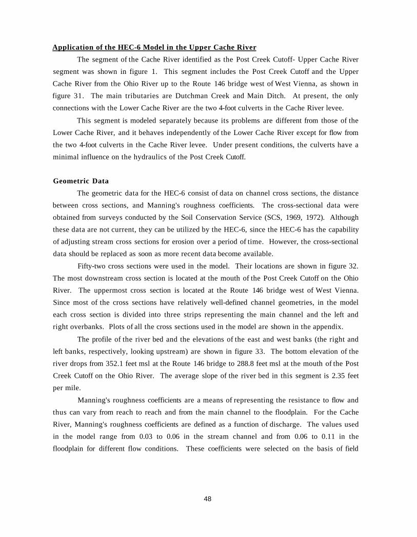
Application of the HEC-6 Model in the Upper Cache River The segment of the Cache River identified as the Post Creek Cutoff- Upper Cache River

segment was shown in figure 1. This segment includes the Post Creek Cutoff and the Upper Cache River from the Ohio River up to the Route 146 bridge west of West Vienna, as shown in figure 31. The main tributaries are Dutchman Creek and Main Ditch. At present, the only connections with the Lower Cache River are the two 4-foot culverts in the Cache River levee.

This segment is modeled separately because its problems are different from those of the Lower Cache River, and it behaves independently of the Lower Cache River except for flow from the two 4-foot culverts in the Cache River levee. Under present conditions, the culverts have a minimal influence on the hydraulics of the Post Creek Cutoff.

Geometric Data The geometric data for the HEC-6 consist of data on channel cross sections, the distance

between cross sections, and Manning's roughness coefficients. The cross-sectional data were obtained from surveys conducted by the Soil Conservation Service (SCS, 1969, 1972). Although these data are not current, they can be utilized by the HEC-6, since the HEC-6 has the capability of adjusting stream cross sections for erosion over a period of time. However, the cross-sectional data should be replaced as soon as more recent data become available.

Fifty-two cross sections were used in the model. Their locations are shown in figure 32. The most downstream cross section is located at the mouth of the Post Creek Cutoff on the Ohio River. The uppermost cross section is located at the Route 146 bridge west of West Vienna. Since most of the cross sections have relatively well-defined channel geometries, in the model each cross section is divided into three strips representing the main channel and the left and right overbanks. Plots of all the cross sections used in the model are shown in the appendix.

The profile of the river bed and the elevations of the east and west banks (the right and left banks, respectively, looking upstream) are shown in figure 33. The bottom elevation of the river drops from 352.1 feet msl at the Route 146 bridge to 288.8 feet msl at the mouth of the Post Creek Cutoff on the Ohio River. The average slope of the river bed in this segment is 2.35 feet per mile.

Manning's roughness coefficients are a means of representing the resistance to flow and thus can vary from reach to reach and from the main channel to the floodplain. For the Cache River, Manning's roughness coefficients are defined as a function of discharge. The values used in the model range from 0.03 to 0.06 in the stream channel and from 0.06 to 0.11 in the floodplain for different flow conditions. These coefficients were selected on the basis of field

48

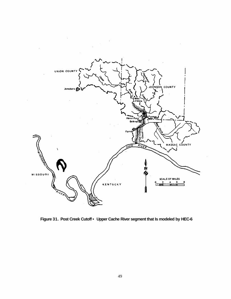
Figure 31. Post Creek Cutoff • Upper Cache River segment that Is modeled by HEC-6

49

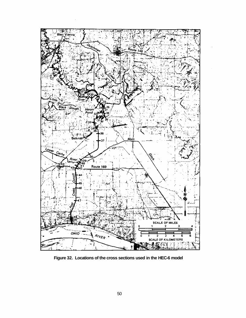
Figure 32. Locations of the cross sections used in the HEC-6 model

50

Figure 33. Profile of the river bed and elevations of the right and left banks looking upstream along the Post Creek Cutoff - Upper Cache River segment

51

inspections, aerial photographs, and engineering judgment, with additional reference to the

roughness coefficients reported by Chow (1959) and Barnes (1967).

Sediment Data Two sets of sediment data are required for the HEC-6: the gradation of bed material at

each cross section, and the inflow sediment load. The inflow sediment load includes the sediment load of the main river and the inflow from tributary streams. A discussion of the sediment data used in the model follows.

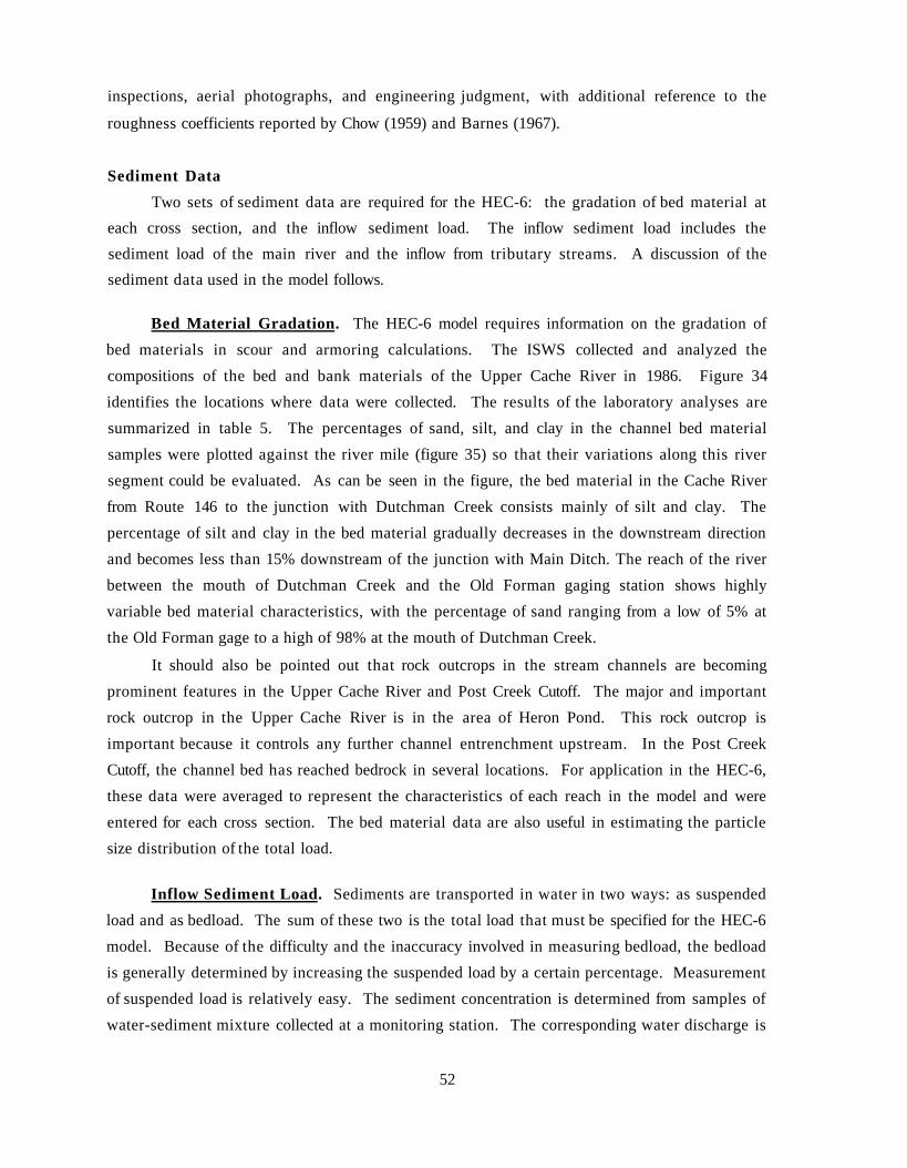
Bed Material Gradation. The HEC-6 model requires information on the gradation of bed materials in scour and armoring calculations. The ISWS collected and analyzed the compositions of the bed and bank materials of the Upper Cache River in 1986. Figure 34 identifies the locations where data were collected. The results of the laboratory analyses are summarized in table 5. The percentages of sand, silt, and clay in the channel bed material samples were plotted against the river mile (figure 35) so that their variations along this river segment could be evaluated. As can be seen in the figure, the bed material in the Cache River from Route 146 to the junction with Dutchman Creek consists mainly of silt and clay. The percentage of silt and clay in the bed material gradually decreases in the downstream direction and becomes less than 15% downstream of the junction with Main Ditch. The reach of the river between the mouth of Dutchman Creek and the Old Forman gaging station shows highly variable bed material characteristics, with the percentage of sand ranging from a low of 5% at the Old Forman gage to a high of 98% at the mouth of Dutchman Creek.

It should also be pointed out that rock outcrops in the stream channels are becoming prominent features in the Upper Cache River and Post Creek Cutoff. The major and important rock outcrop in the Upper Cache River is in the area of Heron Pond. This rock outcrop is important because it controls any further channel entrenchment upstream. In the Post Creek Cutoff, the channel bed has reached bedrock in several locations. For application in the HEC-6, these data were averaged to represent the characteristics of each reach in the model and were entered for each cross section. The bed material data are also useful in estimating the particle size distribution of the total load.

Inflow Sediment Load. Sediments are transported in water in two ways: as suspended load and as bedload. The sum of these two is the total load that must be specified for the HEC-6 model. Because of the difficulty and the inaccuracy involved in measuring bedload, the bedload is generally determined by increasing the suspended load by a certain percentage. Measurement of suspended load is relatively easy. The sediment concentration is determined from samples of water-sediment mixture collected at a monitoring station. The corresponding water discharge is

52

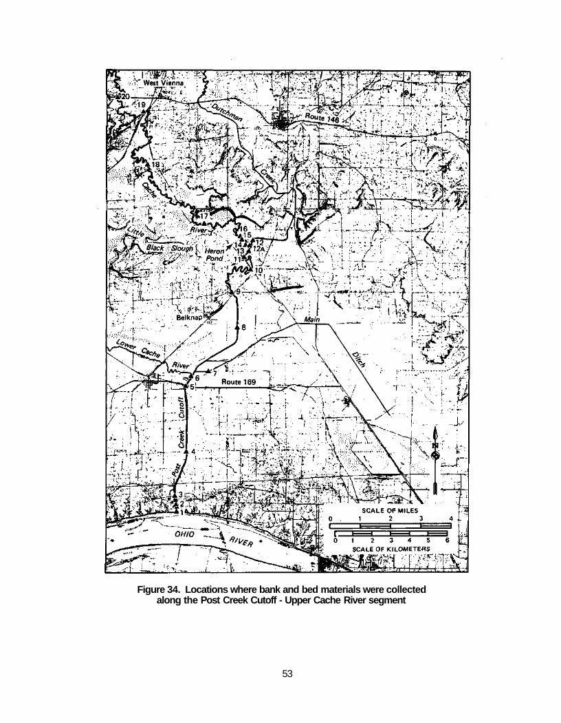
Figure 34. Locations where bank and bed materials were collected along the Post Creek Cutoff - Upper Cache River segment

53

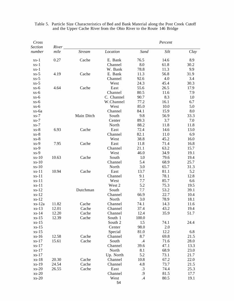
Table 5. Particle Size Characteristics of Bed and Bank Material along the Post Creek Cutoff and the Upper Cache River from the Ohio River to the Route 146 Bridge

Cross Percent Section River number mile Stream Location Sand Silt Clay

xs-1 0.27 Cache E. Bank 76.5 14.6 8.9 xs-1 Channel 8.0 61.8 30.2 xs-1 W. Bank 78.8 11.3 9.9 xs-5 4.19 Cache E. Bank 11.3 56.8 31.9 xs-5 Channel 92.6 4.0 3.4 xs-5 West 24.3 45.4 30.3 xs-6 4.64 Cache East 55.6 26.5 17.9 xs-6 Channel 80.5 11.6 7.9 xs-6 C. Channel 90.7 8.3 1.0 xs-6 W.Channel 77.2 16.1 6.7 xs-6 West 85.0 10.0 5.0 xs-6a Channel 84.1 15.9 8.0 xs-7 Main Ditch South 9.8 56.9 33.3 xs-7 Center 89.3 3.7 7.0 xs-7 North 88.2 11.8 11.8 xs-8 6.93 Cache East 72.4 14.6 13.0 xs-8 Channel 82.1 11.0 6.9 xs-8 West 38.8 45.2 16.0 xs-9 7.95 Cache East 11.8 71.4 16.8 xs-9 Channel 21.1 63.2 15.7 xs-9 West 46.0 34.9 19.1 xs-10 10.63 Cache South 1.0 79.6 19.4 xs-10 Channel 5.4 68.9 25.7 xs-10 North 3.0 65.7 31.3 xs-11 10.94 Cache East 13.7 81.1 5.2 xs-11 Channel 9.1 78.1 12.8 xs-11 West 7.7 85.7 6.6 xs-11 West 2 5.2 75.3 19.5 xs-12 Dutchman South 7.7 53.2 39.1 xs-12 Channel 66.9 22.7 10.4 xs-12 North 3.0 78.9 18.1 xs-12a 11.82 Cache Channel 74.1 14.3 11.6 xs-13 12.01 Cache Channel 37.4 43.2 19.4 xs-14 12.20 Cache Channel 12.4 35.9 51.7 xs-15 12.39 Cache South 1 100.0 xs-15 South 2 1.5 74.1 24.4 xs-15 Center 98.0 2.0 xs-15 Special 81.0 12.2 6.8 xs-16 12.58 Cache Channel 8.7 69.8 21.5 xs-17 15.61 Cache South .4 71.6 28.0 xs-17 Channel 39.6 47.1 13.3 xs-17 North 8.1 68.9 23.0 xs-17 Up. North 5.2 73.1 21.7 xs-18 20.30 Cache Channel 10.8 67.2 22.0 xs-19 24.54 Cache Channel 4.8 73.7 21.5 xs-20 26.55 Cache East .3 74.4 25.3 xs-20 Channel .9 81.5 17.7 xs-20 West .4 80.5 19.1

54

Figure 35. Distributions of sand, silt, and clay In the channel bed materials along the Post Creek Cutoff - Upper Cache River segment

55

either measured at the time of sample collection or determined from rating tables for a known stage. The sediment load that is transported is then determined by multiplying the discharge by the sediment concentration.

The inflow sediment load into a study reach generally consists of two components: the sediment load in the main stream, and that from tributary streams. In this case, the main stream is the Upper Cache River, and the tributary streams are Dutchman Creek and Main Ditch. The following sections present the methods used to determine the sediment loads in the main stem and tributary streams in the Upper Cache River.

Sediment Load in the Main-Stem Stream. The main-stem stream in this segment of the study area is the Upper Cache River. Therefore the suspended sediment load and discharge relationship developed from data collected at a gaging station on the Upper Cache River at Route 146 is used to determine the inflow sediment at the upstream end of the main-stem stream. This gaging station was established by the ISWS for the Cache River basin project, and sediment data are available from June 1985 to the present. The regression equation between suspended sediment load (Qs, in tons per day) and discharge (Qw, in cfs) based on all the available data is

Figure 36 shows these data points, the fitted regression line (equation 19), and the 95% confidence lines. The correlation coefficient and the standard error of estimate are 0.91 and 0.42, respectively.

In addition to this set of data at Route 146, the relationship of sediment and discharge for the Cache River at the Forman gaging station was analyzed. The Forman station is located 16.8 miles downstream from Route 146 and 1.2 miles downstream from the junction of the Cache River with Dutchman Creek (figure 31). Sediment data for this gaging station are available for the period from October 1980 to the present. The regression equation between suspended sediment load (Qs, in tons per day) and discharge (Qw, in cfs) for the gaging station at Forman is given by:

The correlation coefficient is 0.95, and the standard error of estimate is 0.31. This relationship is presented in figure 37. The Forman gage data cover a relatively long period and several floods that have occurred since 1980; therefore the equation derived from the data at Forman is reliable.

The percentages of sand, silt, and clay in the suspended sediment at Route 146 were estimated on the basis of data from laboratory analyses of field samples. Two samples were

56

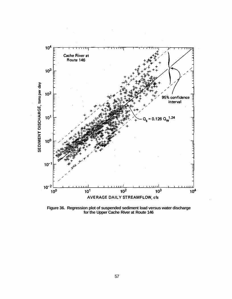
Figure 36. Regression plot of suspended sediment load versus water discharge for the Upper Cache River at Route 146

57

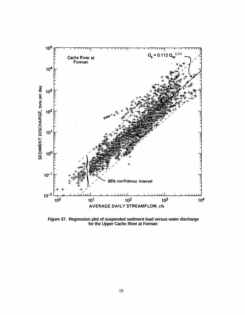
Figure 37. Regression plot of suspended sediment load versus water discharge for the Upper Cache River at Forman

58

collected at Route 146 for particle size analysis, one on May 16, 1986, and the other on August 11, 1986. The results indicated that the May 16 sample consisted of 0.2% sand, 16.2% silt, and 83.6% clay, and the August 11 sample consisted of 0.3% sand, 40.5% silt, and 59.2% clay. The flow conditions were different when these two samples were taken. The May 16 data were taken during a flood (Q = 2690 cfs) with a return period of 1.56 years (determined by analyzing the discharge at the Forman station). On the other hand, the August 11 data were taken during a low-flow condition (Q = 352 cfs). Both samples showed that sand was only a small percentage of the suspended sediment, which is primarily silt and clay. These samples also indicated that the sand content did not increase as the discharge increased at Route 146.

Suspended particle size data at the Forman station were also used to supplement the data at Route 146. Two samples were collected in 1986. One of these samples, collected on May 15 when the discharge was 801 cfs, consisted of 2.8% sand, 48.3% silt, and 48.9% clay. The other one, collected on August 12 when the water discharge was 314 cfs, consisted of 0.4% sand, 40.4% silt, and 59.2% clay. For the Forman station, the sand fraction increased slightly with the discharge. Since very little sand flows into the Cache River at Route 146, the increases in sand at Forman may be due to scouring from the river bed and banks downstream from Route 146. The particle size distribution of the suspended sediment for this segment of the river was taken as the average of the four available samples: sand 1.0%, silt 37%, and clay 62%.

To estimate the total sediment load, the suspended sediment load is generally increased by 5% to 25% to account for the contribution of the bedload to the total load (Simons and Senturk, 1977). Bedload generally consists of larger particles and is transported through saltation, rolling, or sliding in the bed layer. It is not routinely measured. In this study, the available particle sizes from the bed materials were used as a guide for estimating the bedload. On the basis of the bed material characteristics and the particle size distribution of the suspended sediment in this segment of the river, the bedload is assumed to be 5% of the total load. By increasing the suspended load by 5%, the total load for each sediment component is given by the following equations:

Qsd = 0.001 Qwl - 2 4 (for sand) (21)

Qst = 0.490 Qw1.24 (for silt) (22) Qcl = 0.082 Q w

l . 2 4 (for clay) (23)

where Qsd, Qst, and Qcl are the sediment loads for sand, silt, and clay, respectively. The silt and sand fractions are further subdivided into different size classifications in the HEC-6 model for a better description of the particles being transported.

59

Sediment Inflow from Tributary Streams. Three tributaries flow into the Post Creek Cutoff - Upper Cache River segment. They are Dutchman Creek, Main Ditch, and the Lower Cache River (figure 31).

Water and sediment discharges in Dutchman Creek are not monitored continuously. However, because of the similarities of the watersheds of Dutchman Creek and the Upper Cache River upstream of Route 146 in terms of overland slope, land uses, and soil types, the suspended sediment load information for the Cache River at Route 146 is assumed to represent the sediment load from Dutchman Creek. The suspended sediment-discharge relationship for Dutchman Creek is therefore the same as that shown in equation 19. The distribution of suspended sediment particle sizes is also assumed to be the same as that of the Upper Cache River at Route 146.

The bed material characteristics data summarized in table 5 show that the sand fraction is relatively high in Dutchman Creek and immediately downstream of its junction with the Cache River as compared to that found in the Cache River upstream of the junction. This suggests that there is a significant sand input from Dutchman Creek, and it can be assumed that most of that sand is transported as bedload. On the basis of this information, the bedload was estimated to be 10% of the total load and was assumed to be all sand. The corresponding sediment-discharge equations for each of the sediment classes are therefore:

Qsd = 0.001 QW1.24 (for sand) (24)

Qst = 0.051 Qw1.24 (for silt) (25) Qcl = 0.085 Qw1-24 (for clay) (26)

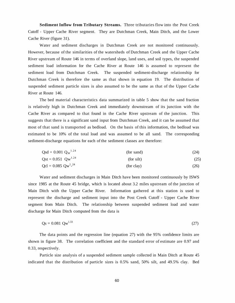
Water and sediment discharges in Main Ditch have been monitored continuously by ISWS since 1985 at the Route 45 bridge, which is located about 3.2 miles upstream of the junction of Main Ditch with the Upper Cache River. Information gathered at this station is used to represent the discharge and sediment input into the Post Creek Cutoff - Upper Cache River segment from Main Ditch. The relationship between suspended sediment load and water discharge for Main Ditch computed from the data is

Qs = 0.081 Qw1.33 (27)

The data points and the regression line (equation 27) with the 95% confidence limits are shown in figure 38. The correlation coefficient and the standard error of estimate are 0.97 and 0.33, respectively.

Particle size analysis of a suspended sediment sample collected in Main Ditch at Route 45 indicated that the distribution of particle sizes is 0.5% sand, 50% silt, and 49.5% clay. Bed

60

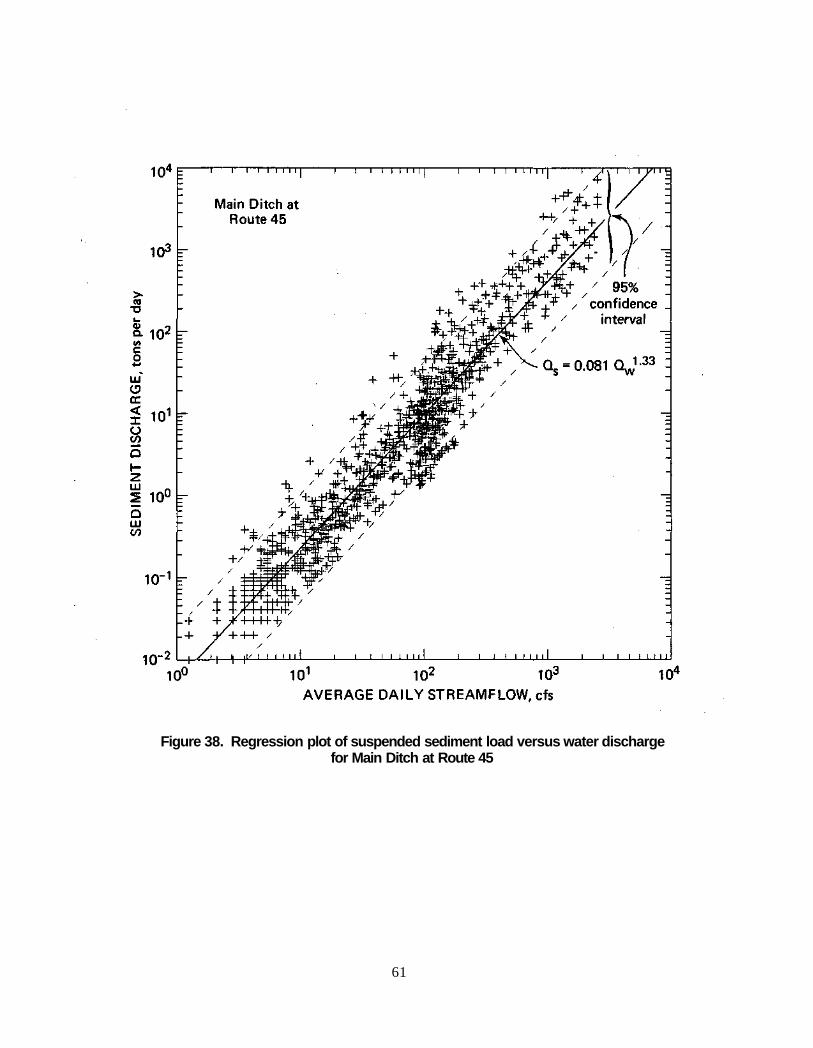
Figure 38. Regression plot of suspended sediment load versus water discharge for Main Ditch at Route 45

61

material samples collected in Main Ditch indicated that the bed material is 89.3% sand (table 5). Therefore, as with the assumption made for Dutchman Creek, the bedload is assumed to consist of sand only and to account for 10% of the total load. Combining this assumption with the distribution of suspended sediment particle sizes and equation 27, the regression equations for sediment inflow in each sediment category are:

Q s d = 0.008 Qw1.33 (for sand) (28) Q s t = 0.04 Q w

l . 3 3 (forsilt) (29)

Qcl = 0.039 Q wl . 3 3 (for clay) (30)

Since the water discharge from the Lower Cache River through the two culverts is generally smaller than the flow in the Upper Cache River, especially during periods of high flows, the sediment inflow from the Lower Cache River to the Post Creek cutoff is ignored for this analysis.

Hydrologic Data Two types of hydrological data are used in this investigation: hydrographs for selected

periods, and flood discharges with specified return periods. The purpose of using floods with specified return periods is to evaluate the flood elevations along the Post Creek Cutoff and Upper Cache River segments, i.e., to determine the water surface elevations at specific locations for given floods. Floods with recurrence intervals of 2, 5, 25, and 100 years were chosen for the analysis. The historic data for the Cache River at Forman were used to compute the magnitudes of these floods since the Forman gage has the longest flow record for the Upper Cache River. The corresponding discharges from tributaries were estimated in accordance with the ratio of their watershed areas to the watershed area at Forman. The ratio for Dutchman Creek was determined to be 0.35; the ratio for Main Ditch was 0.40. Discharge from the Lower Cache River to the Post Creek cutoff is assumed to be 450 cfs, which is the capacity of the culverts when the water surface elevation is at 339 feet above mean sea level. The total discharge at the downstream end of the HEC-6 model reach was obtained by adding the discharges from the Upper Cache River at Forman, Main Ditch at Route 45, and the Lower Cache River at the culverts; The flood discharges at the downstream end and the return periods associated with discharges at Forman were as follows:

62

Discharge at Discharge at Return period Forman downstream end

(years) (cfs) (cfs)

2 3650 5293 5 5950 8628

25 9435 13679 100 12230 17600

The use of different flow records of variable durations in the HEC-6 model aids in investigating the possible scour or sedimentation conditions in the Upper Cache River under various hydrologic conditions. For this purpose, flow hydrographs from Water Years 1929, 1981, 1986, and 1981-1986 were used. Water Year 1929 includes the flood with maximum discharge in the Upper Cache River and thus represents a wet year. Water Year 1981 represents a low-flow year. Water Year 1986 is an average year, with the 26th highest flood on record. The hydrograph for 1981-1986 is used for the purpose of studying long-term trends.

The hydrograph for Water Year 1986 is used to demonstrate the procedures for deriving the total hydrograph and discretizing it for input into HEC-6. Daily discharges are available for the Upper Cache River at Route 146 and at Forman, and for Main Ditch at Route 45. These discharges are plotted in figure 39. The total discharge that flows into the Ohio River is the sum of discharges from the Upper Cache River at Forman, Main Ditch at Route 45, and the Lower Cache River through the culverts. Figure 40 shows the total hydrograph used at the downstream end of the model. The hydrograph is discretized into 22 discharges for input into the HEC-6 model.

The discharge hydrographs for Water Years 1929 and 1981 and for the period 1981-1986 were derived by using the flow records of the Cache River at Forman. The daily discharges of the Upper Cache River at Forman are available from 1924 to the present (USGS, various years). The discharges from tributaries were estimated by using the drainage area ratios and the flow hydrographs of the Cache River at Forman, as discussed earlier. The discharge hydrographs at the downstream end for Water Years 1929, 1981, and 1981-1986 are presented in figures 41 through 43, respectively.

Operating Rules and Downstream Boundary Conditions Operating rules are specified for cross sections with man-made structures designed to

regulate and control water flow and river stages. Formerly, two man-made control structures were located in the Post Creek Cutoff - Upper Cache River segment, one at the Old Forman gaging station and one at Grand Chain Road. The weir structure at the Old Forman gaging station has been damaged as a result of the entrenchment of the stream channel, and it does not

63

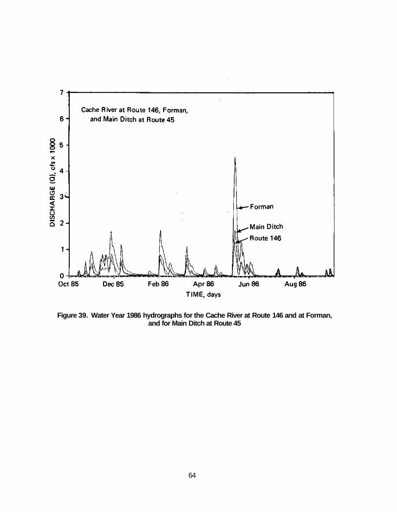
Figure 39. Water Year 1986 hydrographs for the Cache River at Route 146 and at Forman, and for Main Ditch at Route 45

64

Figure 40. Discretized hydrograph for Water Year 1986 used at the downstream end of the Post Creek Cutoff - Upper Cache River model

Figure 41. Discretized hydrograph for Water Year 1929 used at the downstream end of the Post Creek Cutoff - Upper Cache River model

65

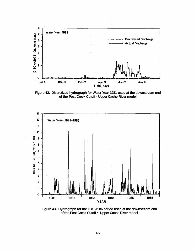
Figure 42. Discretized hydrograph for Water Year 1981 used at the downstream end of the Post Creek Cutoff - Upper Cache River model

Figure 43. Hydrograph for the 1981-1986 period used at the downstream end of the Post Creek Cutoff • Upper Cache River model

66

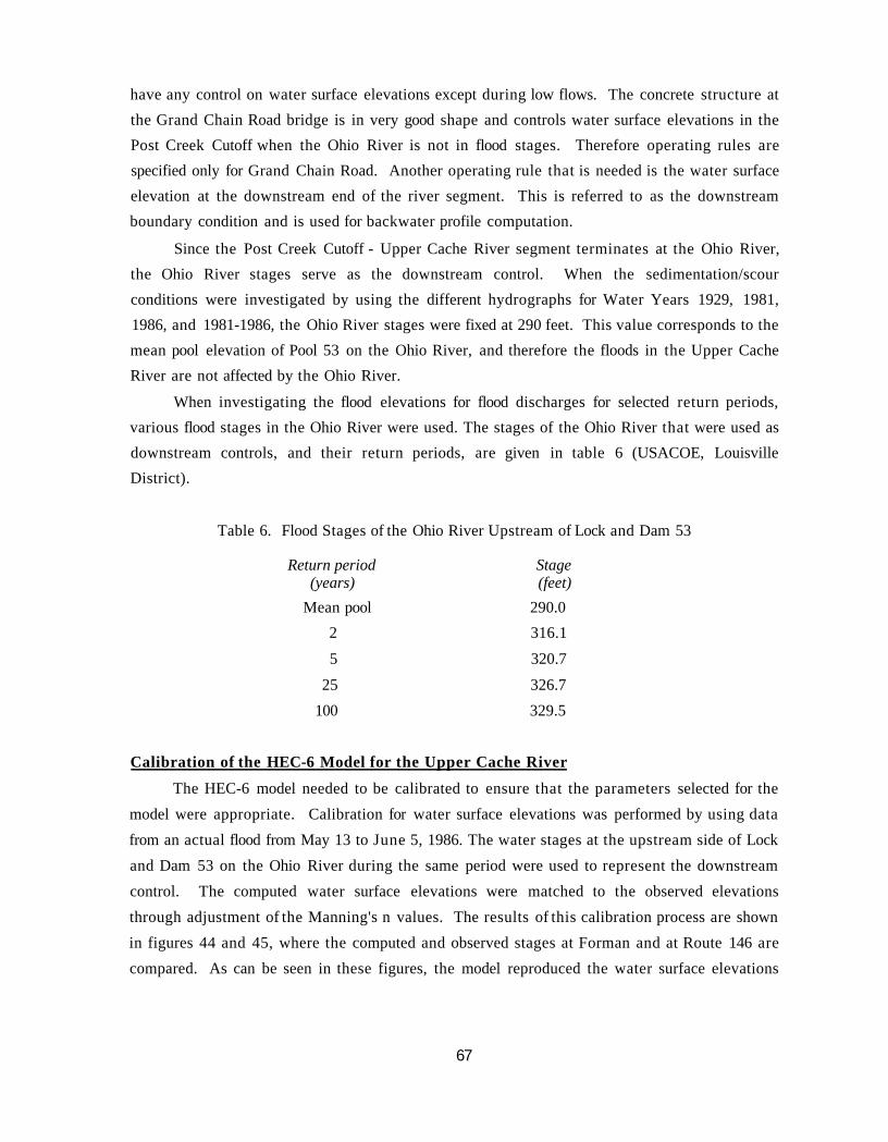
have any control on water surface elevations except during low flows. The concrete structure at the Grand Chain Road bridge is in very good shape and controls water surface elevations in the Post Creek Cutoff when the Ohio River is not in flood stages. Therefore operating rules are specified only for Grand Chain Road. Another operating rule that is needed is the water surface elevation at the downstream end of the river segment. This is referred to as the downstream boundary condition and is used for backwater profile computation.

Since the Post Creek Cutoff - Upper Cache River segment terminates at the Ohio River, the Ohio River stages serve as the downstream control. When the sedimentation/scour conditions were investigated by using the different hydrographs for Water Years 1929, 1981, 1986, and 1981-1986, the Ohio River stages were fixed at 290 feet. This value corresponds to the mean pool elevation of Pool 53 on the Ohio River, and therefore the floods in the Upper Cache River are not affected by the Ohio River.

When investigating the flood elevations for flood discharges for selected return periods, various flood stages in the Ohio River were used. The stages of the Ohio River that were used as downstream controls, and their return periods, are given in table 6 (USACOE, Louisville District).

Table 6. Flood Stages of the Ohio River Upstream of Lock and Dam 53

Return period Stage (years) (feet)

Mean pool 290.0 2 316.1 5 320.7

25 326.7 100 329.5

Calibration of the HEC-6 Model for the Upper Cache River The HEC-6 model needed to be calibrated to ensure that the parameters selected for the

model were appropriate. Calibration for water surface elevations was performed by using data from an actual flood from May 13 to June 5, 1986. The water stages at the upstream side of Lock and Dam 53 on the Ohio River during the same period were used to represent the downstream control. The computed water surface elevations were matched to the observed elevations through adjustment of the Manning's n values. The results of this calibration process are shown in figures 44 and 45, where the computed and observed stages at Forman and at Route 146 are compared. As can be seen in these figures, the model reproduced the water surface elevations

67

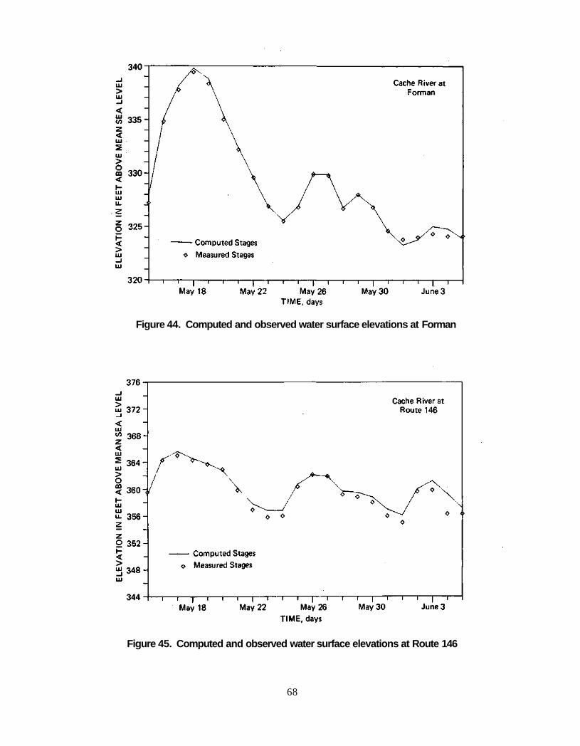
Figure 44. Computed and observed water surface elevations at Forman

Figure 45. Computed and observed water surface elevations at Route 146

68

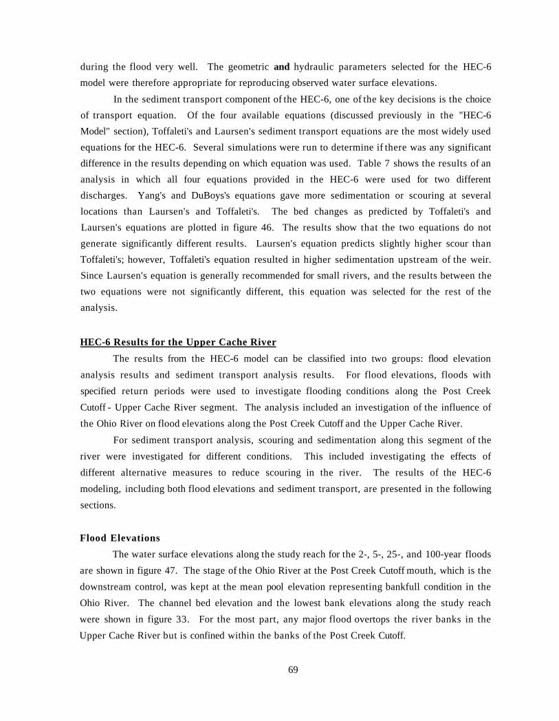
during the flood very well. The geometric and hydraulic parameters selected for the HEC-6 model were therefore appropriate for reproducing observed water surface elevations.

In the sediment transport component of the HEC-6, one of the key decisions is the choice of transport equation. Of the four available equations (discussed previously in the "HEC-6 Model" section), Toffaleti's and Laursen's sediment transport equations are the most widely used equations for the HEC-6. Several simulations were run to determine if there was any significant difference in the results depending on which equation was used. Table 7 shows the results of an analysis in which all four equations provided in the HEC-6 were used for two different discharges. Yang's and DuBoys's equations gave more sedimentation or scouring at several locations than Laursen's and Toffaleti's. The bed changes as predicted by Toffaleti's and Laursen's equations are plotted in figure 46. The results show that the two equations do not generate significantly different results. Laursen's equation predicts slightly higher scour than Toffaleti's; however, Toffaleti's equation resulted in higher sedimentation upstream of the weir. Since Laursen's equation is generally recommended for small rivers, and the results between the two equations were not significantly different, this equation was selected for the rest of the analysis.

HEC-6 Results for the Upper Cache River The results from the HEC-6 model can be classified into two groups: flood elevation

analysis results and sediment transport analysis results. For flood elevations, floods with specified return periods were used to investigate flooding conditions along the Post Creek Cutoff - Upper Cache River segment. The analysis included an investigation of the influence of the Ohio River on flood elevations along the Post Creek Cutoff and the Upper Cache River.

For sediment transport analysis, scouring and sedimentation along this segment of the river were investigated for different conditions. This included investigating the effects of different alternative measures to reduce scouring in the river. The results of the HEC-6 modeling, including both flood elevations and sediment transport, are presented in the following sections.

Flood Elevations The water surface elevations along the study reach for the 2-, 5-, 25-, and 100-year floods

are shown in figure 47. The stage of the Ohio River at the Post Creek Cutoff mouth, which is the downstream control, was kept at the mean pool elevation representing bankfull condition in the Ohio River. The channel bed elevation and the lowest bank elevations along the study reach were shown in figure 33. For the most part, any major flood overtops the river banks in the Upper Cache River but is confined within the banks of the Post Creek Cutoff.

69

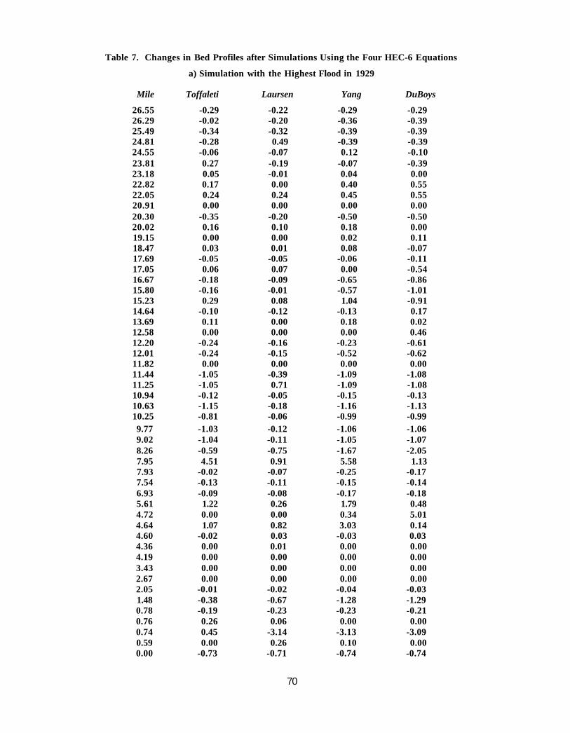
Table 7. Changes in Bed Profiles after Simulations Using the Four HEC-6 Equations

a) Simulation with the Highest Flood in 1929

Mile Toffaleti Laursen Yang DuBoys

26.55 -0.29 -0.22 -0.29 -0.29 26.29 -0.02 -0.20 -0.36 -0.39 25.49 -0.34 -0.32 -0.39 -0.39 24.81 -0.28 0.49 -0.39 -0.39 24.55 -0.06 -0.07 0.12 -0.10 23.81 0.27 -0.19 -0.07 -0.39 23.18 0.05 -0.01 0.04 0.00 22.82 0.17 0.00 0.40 0.55 22.05 0.24 0.24 0.45 0.55 20.91 0.00 0.00 0.00 0.00 20.30 -0.35 -0.20 -0.50 -0.50 20.02 0.16 0.10 0.18 0.00 19.15 0.00 0.00 0.02 0.11 18.47 0.03 0.01 0.08 -0.07 17.69 -0.05 -0.05 -0.06 -0.11 17.05 0.06 0.07 0.00 -0.54 16.67 -0.18 -0.09 -0.65 -0.86 15.80 -0.16 -0.01 -0.57 -1.01 15.23 0.29 0.08 1.04 -0.91 14.64 -0.10 -0.12 -0.13 0.17 13.69 0.11 0.00 0.18 0.02 12.58 0.00 0.00 0.00 0.46 12.20 -0.24 -0.16 -0.23 -0.61 12.01 -0.24 -0.15 -0.52 -0.62 11.82 0.00 0.00 0.00 0.00 11.44 -1.05 -0.39 -1.09 -1.08 11.25 -1.05 0.71 -1.09 -1.08 10.94 -0.12 -0.05 -0.15 -0.13 10.63 -1.15 -0.18 -1.16 -1.13 10.25 -0.81 -0.06 -0.99 -0.99 9.77 -1.03 -0.12 -1.06 -1.06 9.02 -1.04 -0.11 -1.05 -1.07 8.26 -0.59 -0.75 -1.67 -2.05 7.95 4.51 0.91 5.58 1.13 7.93 -0.02 -0.07 -0.25 -0.17 7.54 -0.13 -0.11 -0.15 -0.14 6.93 -0.09 -0.08 -0.17 -0.18 5.61 1.22 0.26 1.79 0.48 4.72 0.00 0.00 0.34 5.01 4.64 1.07 0.82 3.03 0.14 4.60 -0.02 0.03 -0.03 0.03 4.36 0.00 0.01 0.00 0.00 4.19 0.00 0.00 0.00 0.00 3.43 0.00 0.00 0.00 0.00 2.67 0.00 0.00 0.00 0.00 2.05 -0.01 -0.02 -0.04 -0.03 1.48 -0.38 -0.67 -1.28 -1.29 0.78 -0.19 -0.23 -0.23 -0.21 0.76 0.26 0.06 0.00 0.00 0.74 0.45 -3.14 -3.13 -3.09 0.59 0.00 0.26 0.10 0.00 0.00 -0.73 -0.71 -0.74 -0.74

70

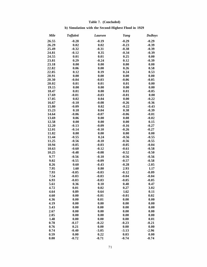
Table 7. (Concluded)

b) Simulation with the Second-Highest Flood in 1929

Mile Toffaleti Laursen Yang DuBoys

26.55 -0.28 -0.19 -0.29 -0.29 26.29 0.02 0.02 -0.23 -0.39 25.49 -0.32 -0.31 -0.38 -0.39 24.81 -0.12 0.35 -0.34 -0.39 24.55 0.01 0.01 0.25 0.00 23.81 0.29 -0.24 0.12 -0.39 23.18 0.00 0.00 0.00 0.00 22.82 0.06 0.00 0.26 0.58 22.05 0.12 0.19 0.24 0.53 20.91 0.00 0.00 0.00 0.00 20.30 -0.04 -0.03 -0.06 -0.05 20.02 0.01 0.01 0.01 0.00 19.15 0.00 0.00 0.00 0.00 18.47 0.01 0.00 0.01 -0.05 17.69 -0.01 -0.03 -0.01 0.00 17.05 0.02 0.04 0.00 -0.22 16.67 -0.10 -0.08 -0.26 -0.36 15.80 -0.09 0.02 -0.22 -0.43 15.23 0.18 0.04 0.38 -0.39 14.64 -0.06 -0.07 -0.06 -0.01 13.69 0.06 0.00 0.08 -0.02 12.58 0.00 0.00 0.00 0.15 12.20 -0.13 -0.09 -0.16 -0.27 12.01 -0.14 -0.10 -0.26 -0.27 11.82 0.00 0.00 0.00 0.00 11.44 -0.55 0.24 -0.56 -0.55 11.25 -0.56 -0.10 -0.56 -0.55 10.94 -0.05 -0.03 -0.05 -0.04 10.63 -0.60 -0.12 -0.61 -0.58 10.25 -0.48 -0.08 -0.52 -0.50 9.77 -0.56 -0.10 -0.56 -0.56 9.02 -0.55 -0.09 -0.57 -0.58 8.26 0.60 -0.43 -0.28 -2.05 7.95 1.60 0.80 2.93 1.17 7.93 -0.05 -0.03 -0.12 -0.09 7.54 -0.03 -0.03 -0.04 -0.04 6.93 -0.03 -0.03 -0.05 -0.05 5.61 0.36 0.10 0.48 0.47 4.72 0.01 0.02 0.27 3.02 4.64 0.89 0.64 1.62 0.11 4.60 0.00 -0.01 -0.01 0.02 4.36 0.00 0.01 0.00 0.00 4.19 0.00 0.00 0.00 0.00 3.43 0.00 0.00 0.00 0.00 2.67 0.00 0.00 0.00 0.00 2.05 0.00 0.00 0.00 0.00 1.48 0.00 0.00 0.00 0.01 0.78 -0.17 -0.22 -0.23 -0.21 0.76 0.21 0.00 0.00 0.00 0.74 -0.40 -3.05 -3.13 -2.96 0.59 0.00 0.22 0.03 0.00 0.00 -0.72 -0.71 -0.74 -0.74

71

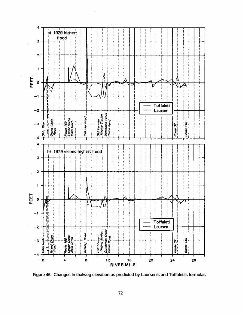
Figure 46. Changes In thalweg elevation as predicted by Laursen's and Toffaleti's formulas

72

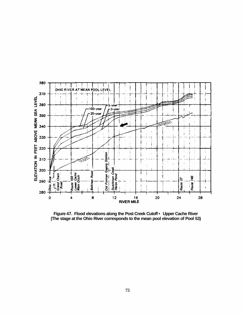
Figure 47. Flood elevations along the Post Creek Cutoff • Upper Cache River (The stage at the Ohio River corresponds to the mean pool elevation of Pool 53)

73

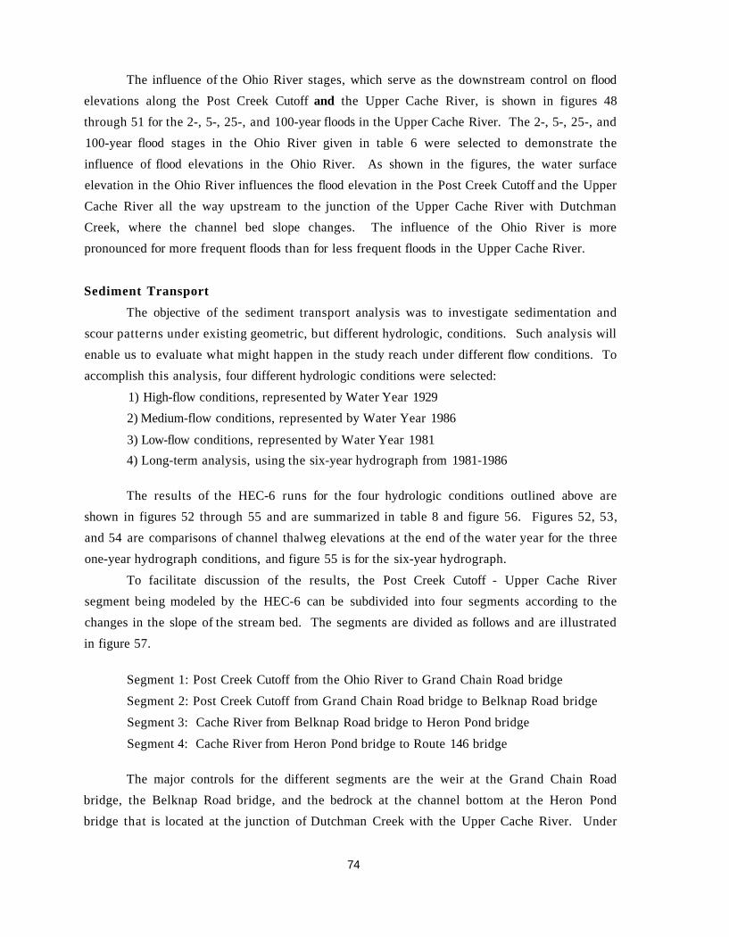
The influence of the Ohio River stages, which serve as the downstream control on flood elevations along the Post Creek Cutoff and the Upper Cache River, is shown in figures 48 through 51 for the 2-, 5-, 25-, and 100-year floods in the Upper Cache River. The 2-, 5-, 25-, and 100-year flood stages in the Ohio River given in table 6 were selected to demonstrate the influence of flood elevations in the Ohio River. As shown in the figures, the water surface elevation in the Ohio River influences the flood elevation in the Post Creek Cutoff and the Upper Cache River all the way upstream to the junction of the Upper Cache River with Dutchman Creek, where the channel bed slope changes. The influence of the Ohio River is more pronounced for more frequent floods than for less frequent floods in the Upper Cache River.

Sediment Transport The objective of the sediment transport analysis was to investigate sedimentation and

scour patterns under existing geometric, but different hydrologic, conditions. Such analysis will enable us to evaluate what might happen in the study reach under different flow conditions. To accomplish this analysis, four different hydrologic conditions were selected:

1) High-flow conditions, represented by Water Year 1929 2) Medium-flow conditions, represented by Water Year 1986

3) Low-flow conditions, represented by Water Year 1981 4) Long-term analysis, using the six-year hydrograph from 1981-1986

The results of the HEC-6 runs for the four hydrologic conditions outlined above are shown in figures 52 through 55 and are summarized in table 8 and figure 56. Figures 52, 53, and 54 are comparisons of channel thalweg elevations at the end of the water year for the three one-year hydrograph conditions, and figure 55 is for the six-year hydrograph.

To facilitate discussion of the results, the Post Creek Cutoff - Upper Cache River segment being modeled by the HEC-6 can be subdivided into four segments according to the changes in the slope of the stream bed. The segments are divided as follows and are illustrated in figure 57.

Segment 1: Post Creek Cutoff from the Ohio River to Grand Chain Road bridge Segment 2: Post Creek Cutoff from Grand Chain Road bridge to Belknap Road bridge Segment 3: Cache River from Belknap Road bridge to Heron Pond bridge Segment 4: Cache River from Heron Pond bridge to Route 146 bridge

The major controls for the different segments are the weir at the Grand Chain Road bridge, the Belknap Road bridge, and the bedrock at the channel bottom at the Heron Pond bridge that is located at the junction of Dutchman Creek with the Upper Cache River. Under

74

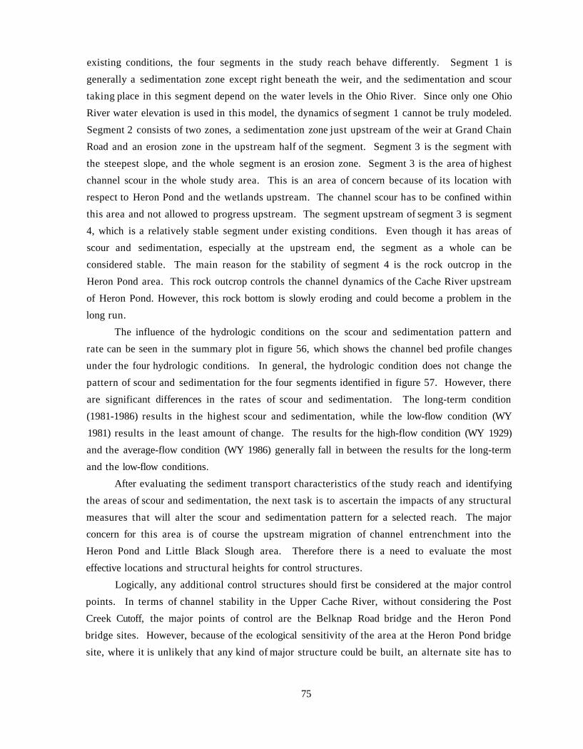
existing conditions, the four segments in the study reach behave differently. Segment 1 is generally a sedimentation zone except right beneath the weir, and the sedimentation and scour taking place in this segment depend on the water levels in the Ohio River. Since only one Ohio River water elevation is used in this model, the dynamics of segment 1 cannot be truly modeled. Segment 2 consists of two zones, a sedimentation zone just upstream of the weir at Grand Chain Road and an erosion zone in the upstream half of the segment. Segment 3 is the segment with the steepest slope, and the whole segment is an erosion zone. Segment 3 is the area of highest channel scour in the whole study area. This is an area of concern because of its location with respect to Heron Pond and the wetlands upstream. The channel scour has to be confined within this area and not allowed to progress upstream. The segment upstream of segment 3 is segment 4, which is a relatively stable segment under existing conditions. Even though it has areas of scour and sedimentation, especially at the upstream end, the segment as a whole can be considered stable. The main reason for the stability of segment 4 is the rock outcrop in the Heron Pond area. This rock outcrop controls the channel dynamics of the Cache River upstream of Heron Pond. However, this rock bottom is slowly eroding and could become a problem in the long run.

The influence of the hydrologic conditions on the scour and sedimentation pattern and rate can be seen in the summary plot in figure 56, which shows the channel bed profile changes under the four hydrologic conditions. In general, the hydrologic condition does not change the pattern of scour and sedimentation for the four segments identified in figure 57. However, there are significant differences in the rates of scour and sedimentation. The long-term condition (1981-1986) results in the highest scour and sedimentation, while the low-flow condition (WY 1981) results in the least amount of change. The results for the high-flow condition (WY 1929) and the average-flow condition (WY 1986) generally fall in between the results for the long-term and the low-flow conditions.

After evaluating the sediment transport characteristics of the study reach and identifying the areas of scour and sedimentation, the next task is to ascertain the impacts of any structural measures that will alter the scour and sedimentation pattern for a selected reach. The major concern for this area is of course the upstream migration of channel entrenchment into the Heron Pond and Little Black Slough area. Therefore there is a need to evaluate the most effective locations and structural heights for control structures.

Logically, any additional control structures should first be considered at the major control points. In terms of channel stability in the Upper Cache River, without considering the Post Creek Cutoff, the major points of control are the Belknap Road bridge and the Heron Pond bridge sites. However, because of the ecological sensitivity of the area at the Heron Pond bridge site, where it is unlikely that any kind of major structure could be built, an alternate site has to

75

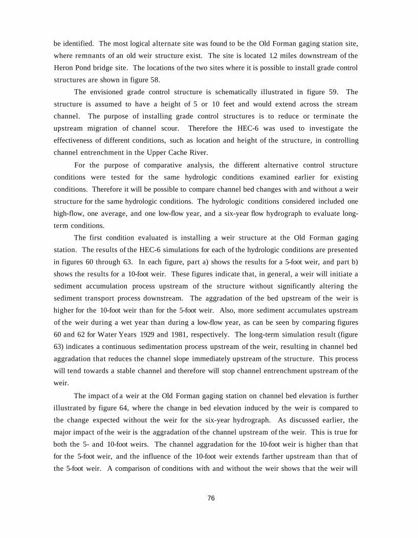
be identified. The most logical alternate site was found to be the Old Forman gaging station site, where remnants of an old weir structure exist. The site is located 1.2 miles downstream of the Heron Pond bridge site. The locations of the two sites where it is possible to install grade control structures are shown in figure 58.

The envisioned grade control structure is schematically illustrated in figure 59. The structure is assumed to have a height of 5 or 10 feet and would extend across the stream channel. The purpose of installing grade control structures is to reduce or terminate the upstream migration of channel scour. Therefore the HEC-6 was used to investigate the effectiveness of different conditions, such as location and height of the structure, in controlling channel entrenchment in the Upper Cache River.

For the purpose of comparative analysis, the different alternative control structure conditions were tested for the same hydrologic conditions examined earlier for existing conditions. Therefore it will be possible to compare channel bed changes with and without a weir structure for the same hydrologic conditions. The hydrologic conditions considered included one high-flow, one average, and one low-flow year, and a six-year flow hydrograph to evaluate long-term conditions.

The first condition evaluated is installing a weir structure at the Old Forman gaging station. The results of the HEC-6 simulations for each of the hydrologic conditions are presented in figures 60 through 63. In each figure, part a) shows the results for a 5-foot weir, and part b) shows the results for a 10-foot weir. These figures indicate that, in general, a weir will initiate a sediment accumulation process upstream of the structure without significantly altering the sediment transport process downstream. The aggradation of the bed upstream of the weir is higher for the 10-foot weir than for the 5-foot weir. Also, more sediment accumulates upstream of the weir during a wet year than during a low-flow year, as can be seen by comparing figures 60 and 62 for Water Years 1929 and 1981, respectively. The long-term simulation result (figure 63) indicates a continuous sedimentation process upstream of the weir, resulting in channel bed aggradation that reduces the channel slope immediately upstream of the structure. This process will tend towards a stable channel and therefore will stop channel entrenchment upstream of the weir.

The impact of a weir at the Old Forman gaging station on channel bed elevation is further illustrated by figure 64, where the change in bed elevation induced by the weir is compared to the change expected without the weir for the six-year hydrograph. As discussed earlier, the major impact of the weir is the aggradation of the channel upstream of the weir. This is true for both the 5- and 10-foot weirs. The channel aggradation for the 10-foot weir is higher than that for the 5-foot weir, and the influence of the 10-foot weir extends farther upstream than that of the 5-foot weir. A comparison of conditions with and without the weir shows that the weir will

76

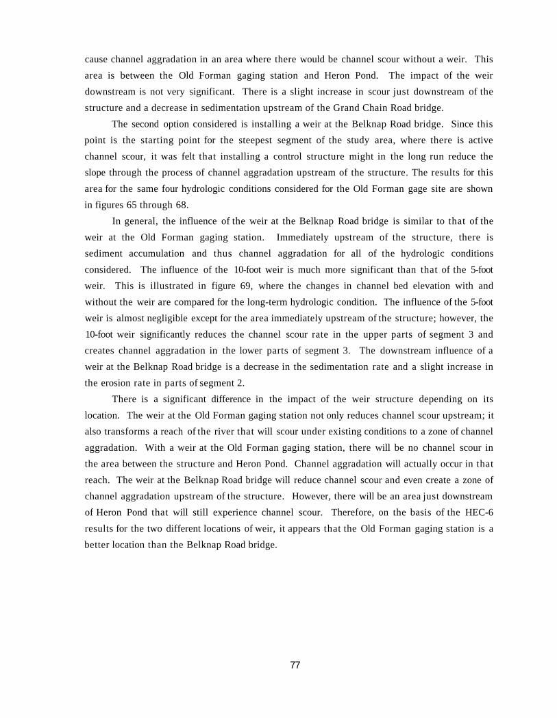
cause channel aggradation in an area where there would be channel scour without a weir. This area is between the Old Forman gaging station and Heron Pond. The impact of the weir downstream is not very significant. There is a slight increase in scour just downstream of the structure and a decrease in sedimentation upstream of the Grand Chain Road bridge.

The second option considered is installing a weir at the Belknap Road bridge. Since this point is the starting point for the steepest segment of the study area, where there is active channel scour, it was felt that installing a control structure might in the long run reduce the slope through the process of channel aggradation upstream of the structure. The results for this area for the same four hydrologic conditions considered for the Old Forman gage site are shown in figures 65 through 68.

In general, the influence of the weir at the Belknap Road bridge is similar to that of the weir at the Old Forman gaging station. Immediately upstream of the structure, there is sediment accumulation and thus channel aggradation for all of the hydrologic conditions considered. The influence of the 10-foot weir is much more significant than that of the 5-foot weir. This is illustrated in figure 69, where the changes in channel bed elevation with and without the weir are compared for the long-term hydrologic condition. The influence of the 5-foot weir is almost negligible except for the area immediately upstream of the structure; however, the 10-foot weir significantly reduces the channel scour rate in the upper parts of segment 3 and creates channel aggradation in the lower parts of segment 3. The downstream influence of a weir at the Belknap Road bridge is a decrease in the sedimentation rate and a slight increase in the erosion rate in parts of segment 2.

There is a significant difference in the impact of the weir structure depending on its location. The weir at the Old Forman gaging station not only reduces channel scour upstream; it also transforms a reach of the river that will scour under existing conditions to a zone of channel aggradation. With a weir at the Old Forman gaging station, there will be no channel scour in the area between the structure and Heron Pond. Channel aggradation will actually occur in that reach. The weir at the Belknap Road bridge will reduce channel scour and even create a zone of channel aggradation upstream of the structure. However, there will be an area just downstream of Heron Pond that will still experience channel scour. Therefore, on the basis of the HEC-6 results for the two different locations of weir, it appears that the Old Forman gaging station is a better location than the Belknap Road bridge.

77

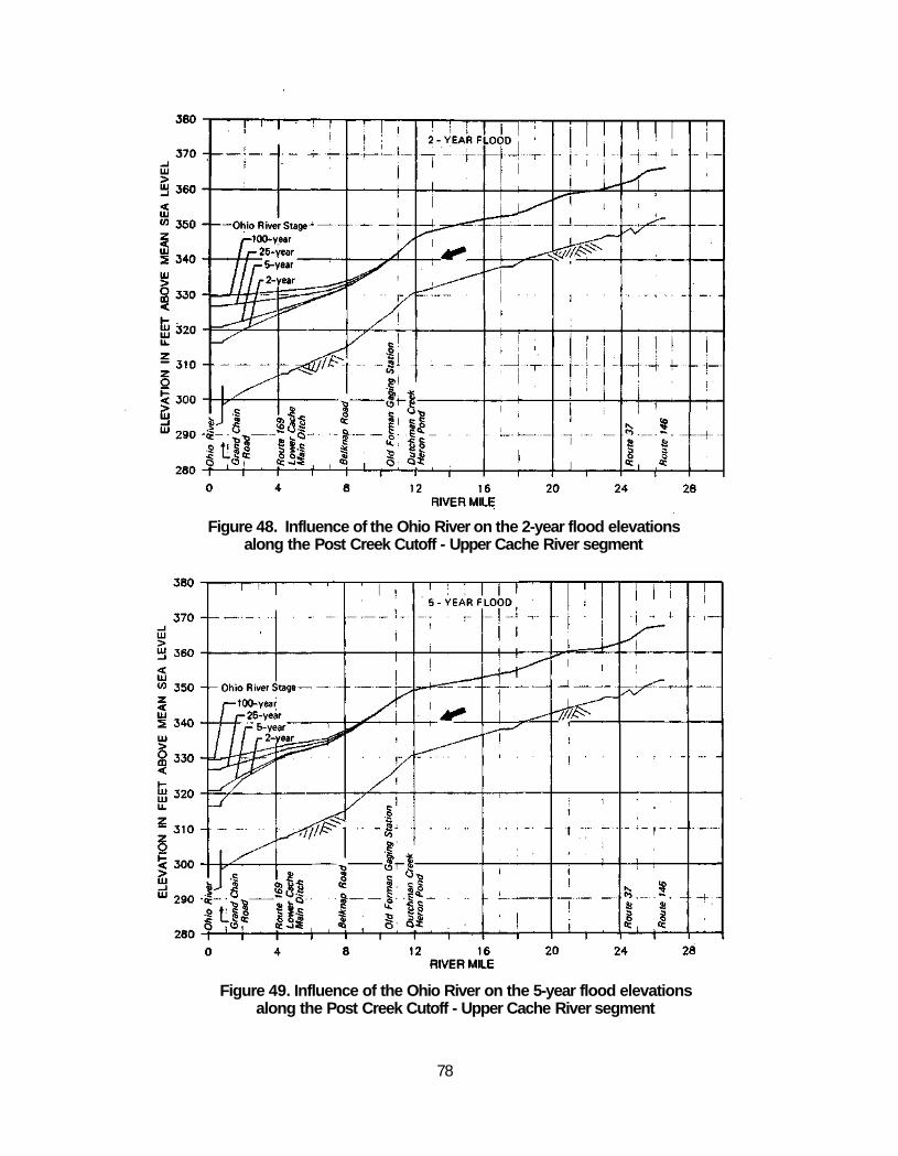
Figure 48. Influence of the Ohio River on the 2-year flood elevations along the Post Creek Cutoff - Upper Cache River segment

Figure 49. Influence of the Ohio River on the 5-year flood elevations along the Post Creek Cutoff - Upper Cache River segment

78

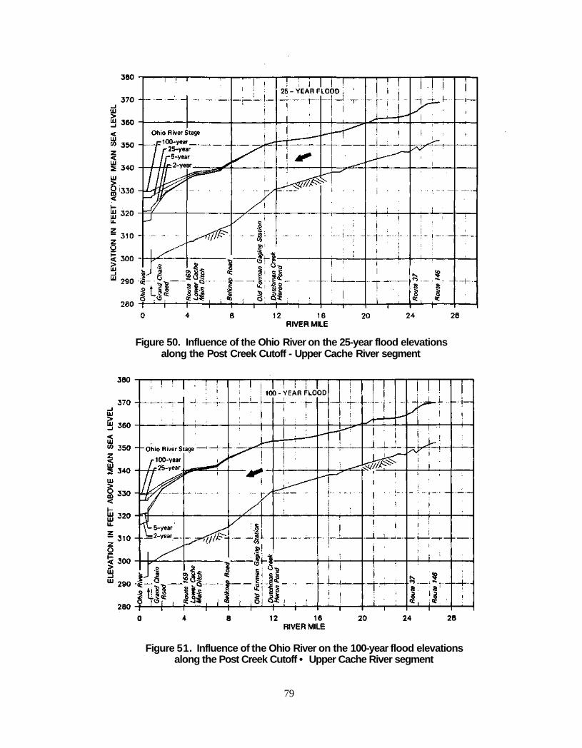
Figure 50. Influence of the Ohio River on the 25-year flood elevations along the Post Creek Cutoff - Upper Cache River segment

Figure 51. Influence of the Ohio River on the 100-year flood elevations along the Post Creek Cutoff • Upper Cache River segment

79

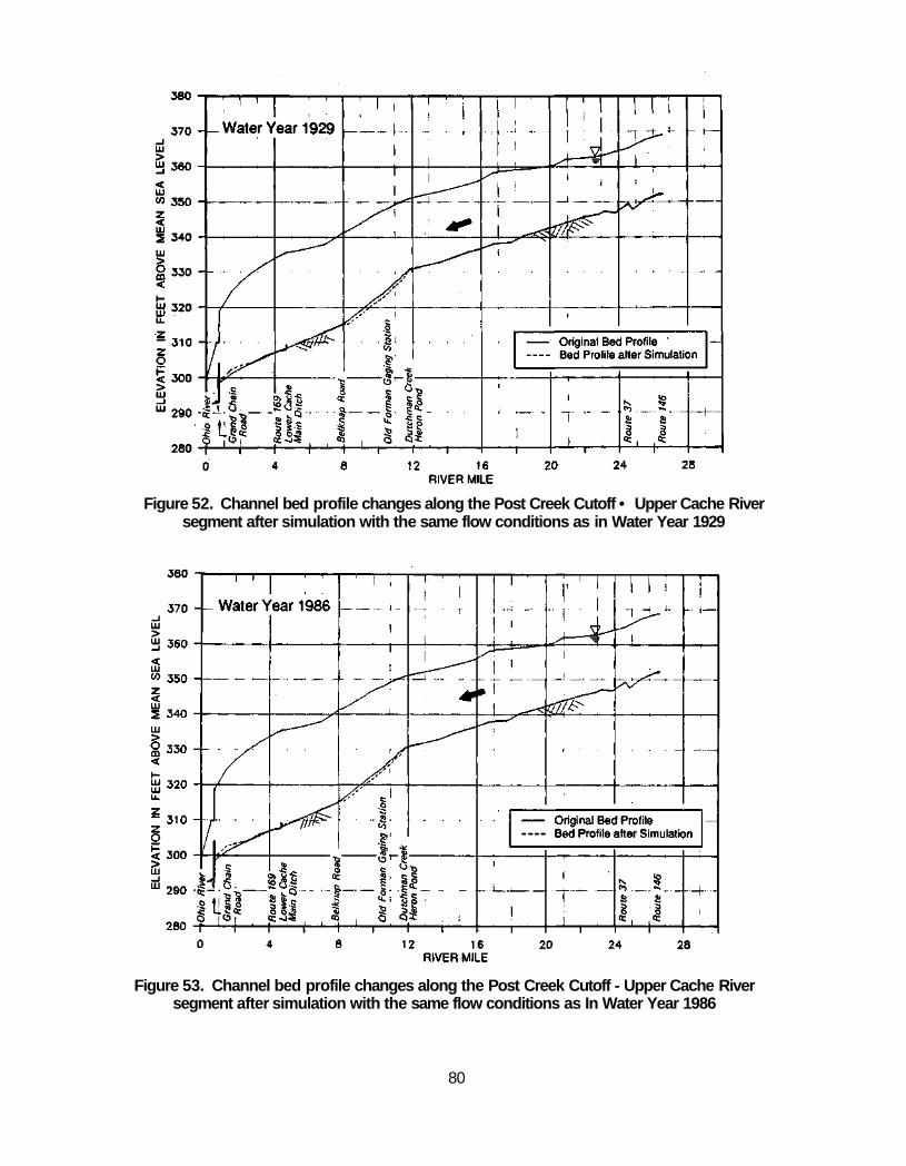
Figure 52. Channel bed profile changes along the Post Creek Cutoff • Upper Cache River segment after simulation with the same flow conditions as in Water Year 1929

Figure 53. Channel bed profile changes along the Post Creek Cutoff - Upper Cache River segment after simulation with the same flow conditions as In Water Year 1986

80

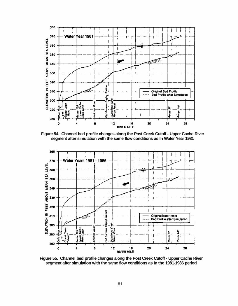
Figure 54. Channel bed profile changes along the Post Creek Cutoff - Upper Cache River segment after simulation with the same flow conditions as In Water Year 1981

Figure 55. Channel bed profile changes along the Post Creek Cutoff - Upper Cache River segment after simulation with the same flow conditions as In the 1981-1986 period

81

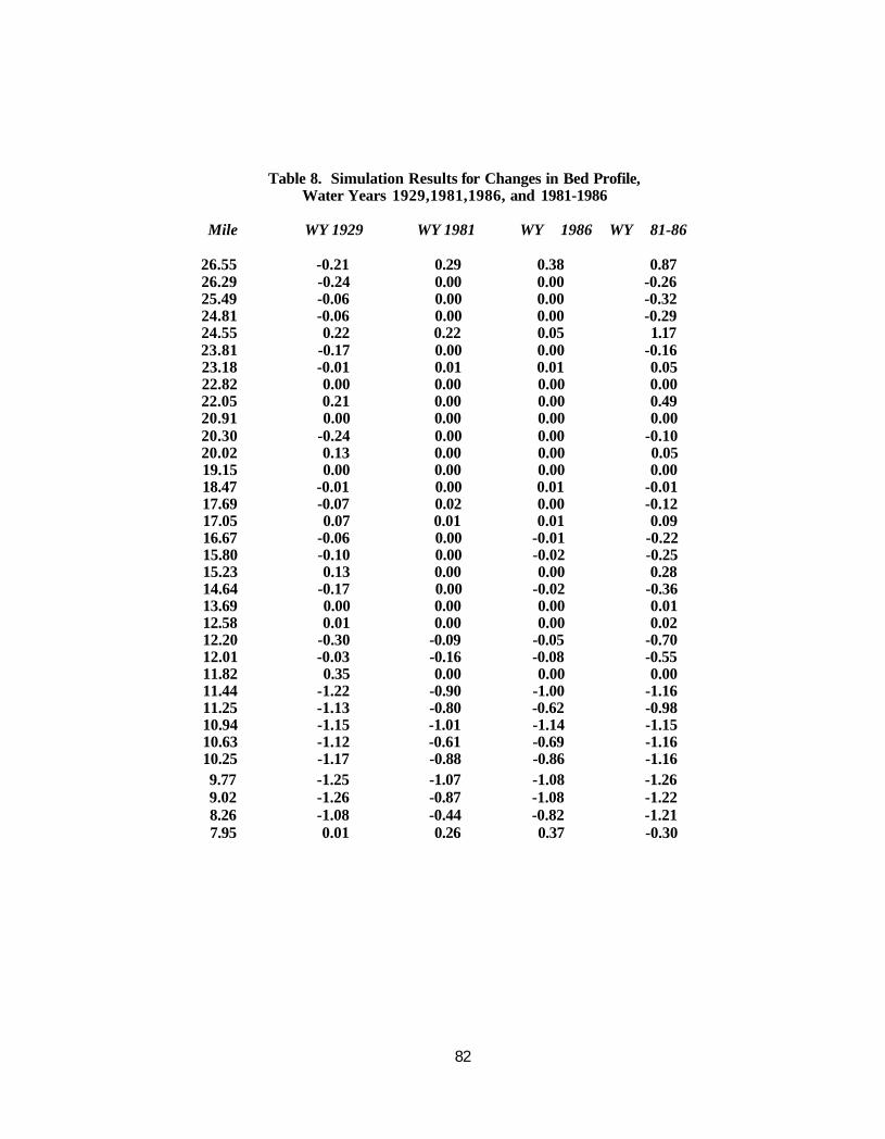
Table 8. Simulation Results for Changes in Bed Profile, Water Years 1929,1981,1986, and 1981-1986

Mile WY 1929 WY 1981 WY 1986 WY 81-86

26.55 -0.21 0.29 0.38 0.87 26.29 -0.24 0.00 0.00 -0.26 25.49 -0.06 0.00 0.00 -0.32 24.81 -0.06 0.00 0.00 -0.29 24.55 0.22 0.22 0.05 1.17 23.81 -0.17 0.00 0.00 -0.16 23.18 -0.01 0.01 0.01 0.05 22.82 0.00 0.00 0.00 0.00 22.05 0.21 0.00 0.00 0.49 20.91 0.00 0.00 0.00 0.00 20.30 -0.24 0.00 0.00 -0.10 20.02 0.13 0.00 0.00 0.05 19.15 0.00 0.00 0.00 0.00 18.47 -0.01 0.00 0.01 -0.01 17.69 -0.07 0.02 0.00 -0.12 17.05 0.07 0.01 0.01 0.09 16.67 -0.06 0.00 -0.01 -0.22 15.80 -0.10 0.00 -0.02 -0.25 15.23 0.13 0.00 0.00 0.28 14.64 -0.17 0.00 -0.02 -0.36 13.69 0.00 0.00 0.00 0.01 12.58 0.01 0.00 0.00 0.02 12.20 -0.30 -0.09 -0.05 -0.70 12.01 -0.03 -0.16 -0.08 -0.55 11.82 0.35 0.00 0.00 0.00 11.44 -1.22 -0.90 -1.00 -1.16 11.25 -1.13 -0.80 -0.62 -0.98 10.94 -1.15 -1.01 -1.14 -1.15 10.63 -1.12 -0.61 -0.69 -1.16 10.25 -1.17 -0.88 -0.86 -1.16 9.77 -1.25 -1.07 -1.08 -1.26 9.02 -1.26 -0.87 -1.08 -1.22 8.26 -1.08 -0.44 -0.82 -1.21 7.95 0.01 0.26 0.37 -0.30

82

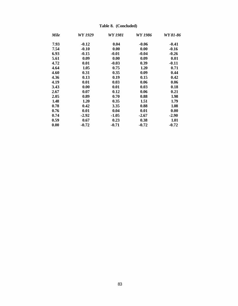
Table 8. (Concluded)

Mile WY 1929 WY 1981 WY 1986 WY 81-86

7.93 -0.12 0.04 -0.06 -0.41 7.54 -0.10 0.00 0.00 -0.16 6.93 -0.15 -0.01 -0.04 -0.26 5.61 0.09 0.00 0.09 0.01 4.72 0.01 -0.03 0.39 -0.11 4.64 1.05 0.75 1.20 0.71 4.60 0.31 0.35 0.09 0.44 4.36 0.13 0.19 0.15 0.42 4.19 0.01 0.03 0.06 0.06 3.43 0.00 0.01 0.03 0.18 2.67 0.07 0.12 0.06 0.21 2.05 0.89 0.70 0.88 1.98 1.48 1.20 0.35 1.51 1.79 0.78 0.42 3.35 0.88 1.08 0.76 0.01 0.04 0.01 0.00 0.74 -2.92 -1.05 -2.67 -2.90 0.59 0.67 0.23 0.38 1.01 0.00 -0.72 -0.71 -0.72 -0.72

83

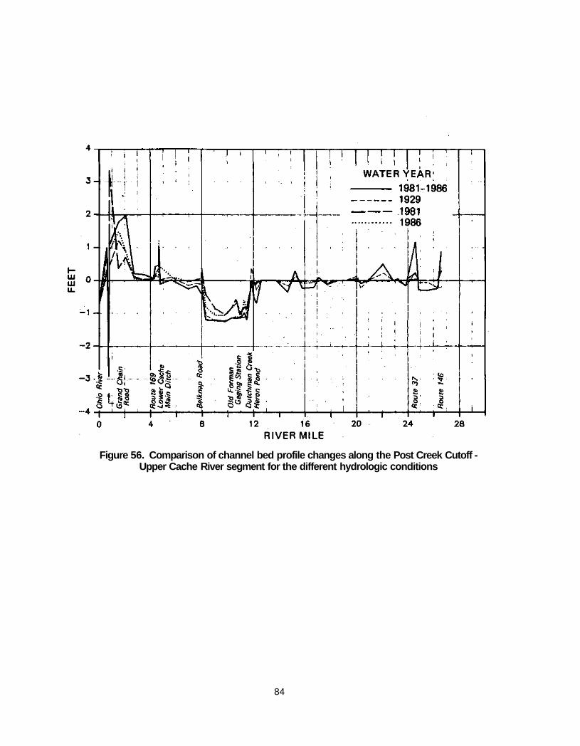
Figure 56. Comparison of channel bed profile changes along the Post Creek Cutoff -Upper Cache River segment for the different hydrologic conditions

84

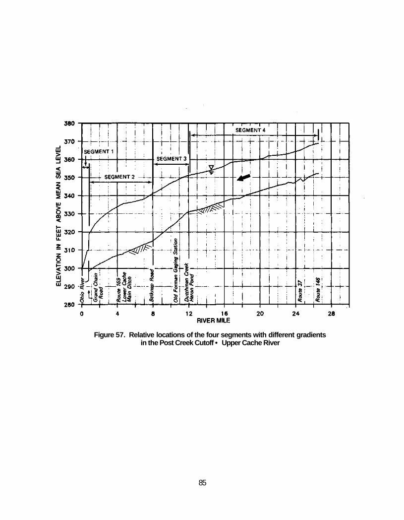
Figure 57. Relative locations of the four segments with different gradients in the Post Creek Cutoff • Upper Cache River

85

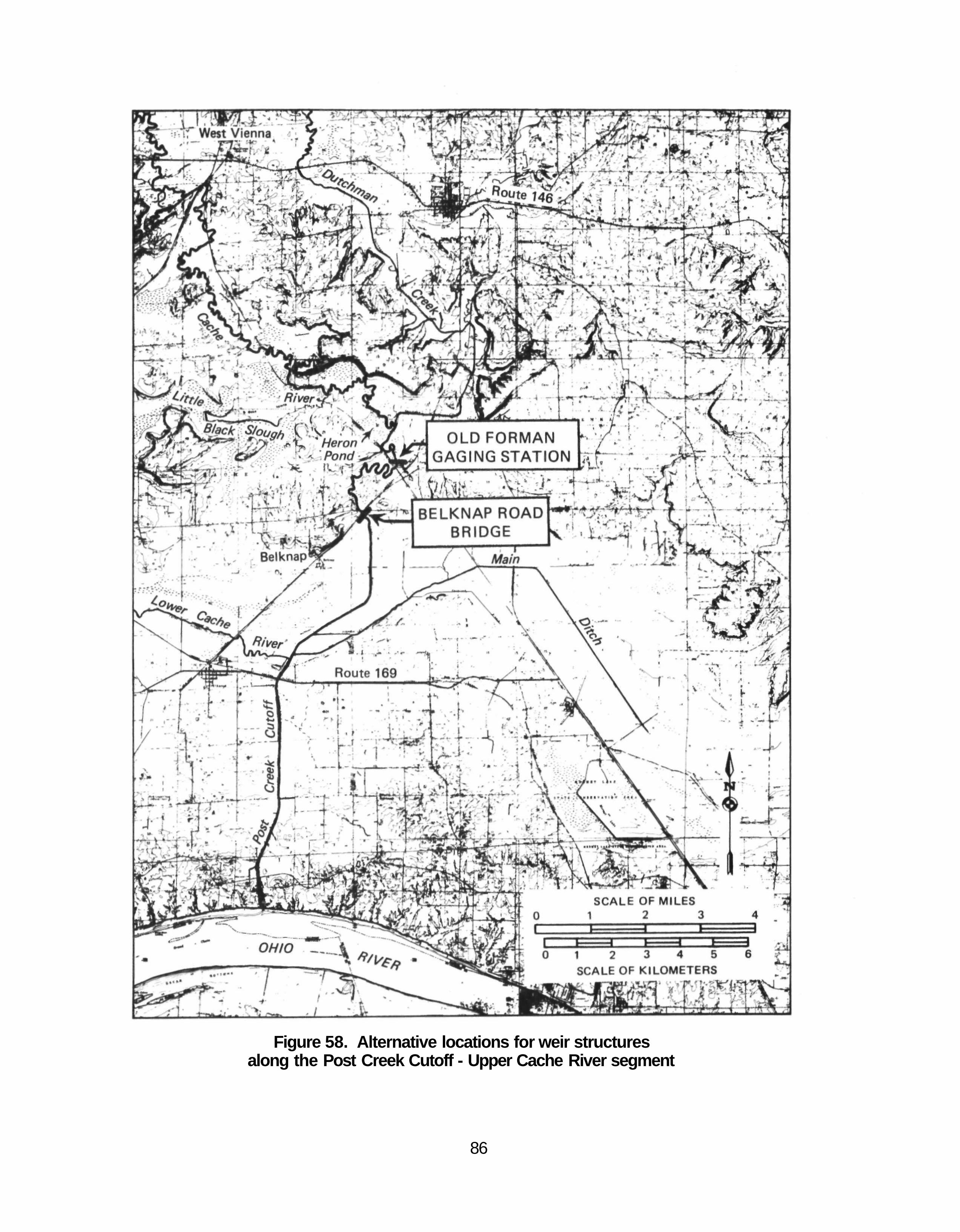
Figure 58. Alternative locations for weir structures along the Post Creek Cutoff - Upper Cache River segment

86

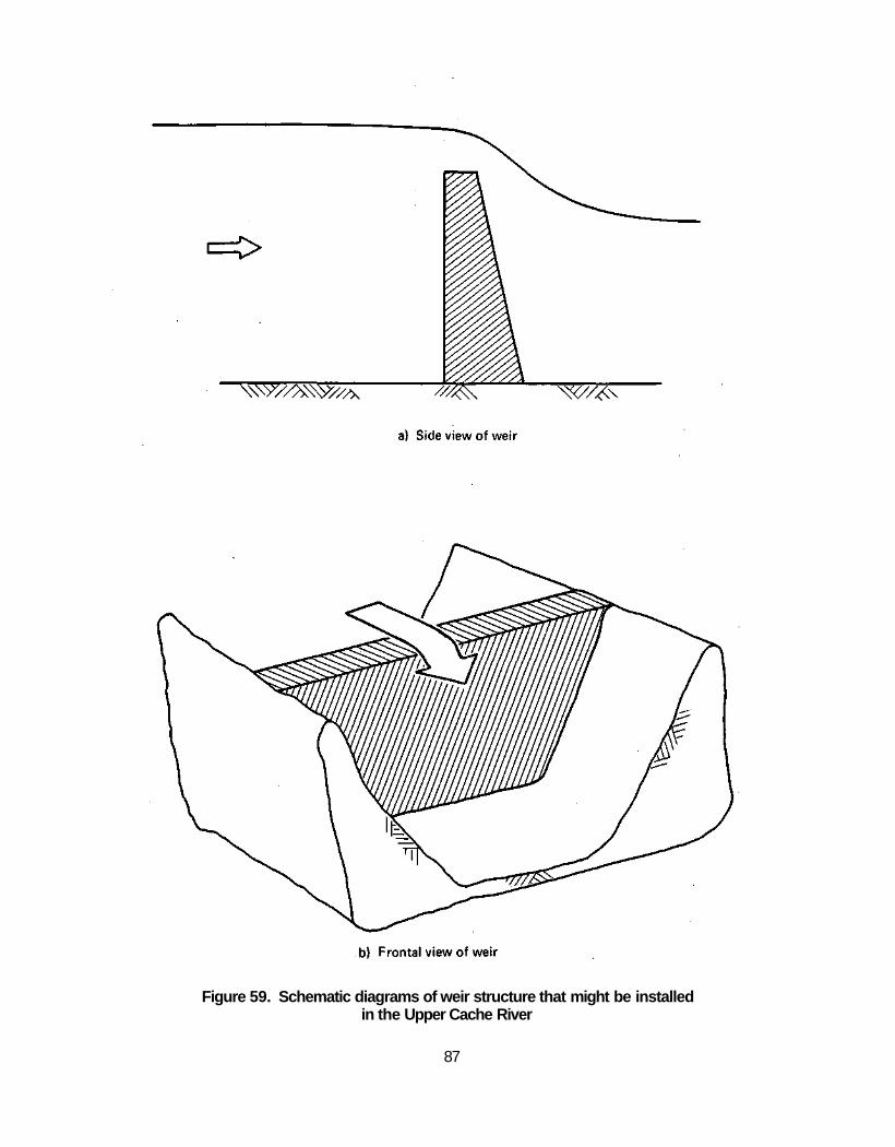
Figure 59. Schematic diagrams of weir structure that might be installed in the Upper Cache River

87

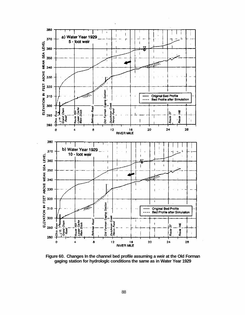
Figure 60. Changes In the channel bed profile assuming a weir at the Old Forman gaging station for hydrologlc conditions the same as in Water Year 1929

88

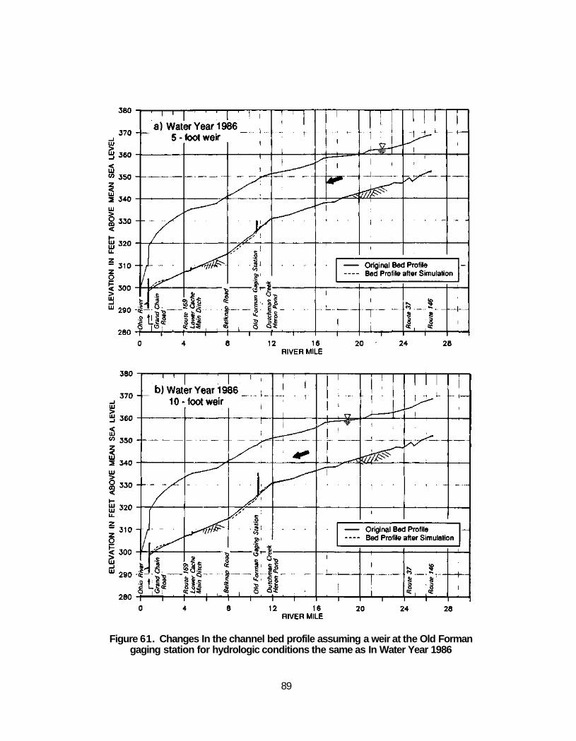
Figure 61. Changes In the channel bed profile assuming a weir at the Old Forman gaging station for hydrologic conditions the same as In Water Year 1986

89

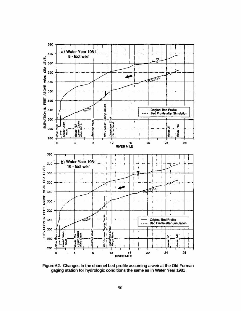
Figure 62. Changes In the channel bed profile assuming a weir at the Old Forman gaging station for hydrologic conditions the same as in Water Year 1981

90

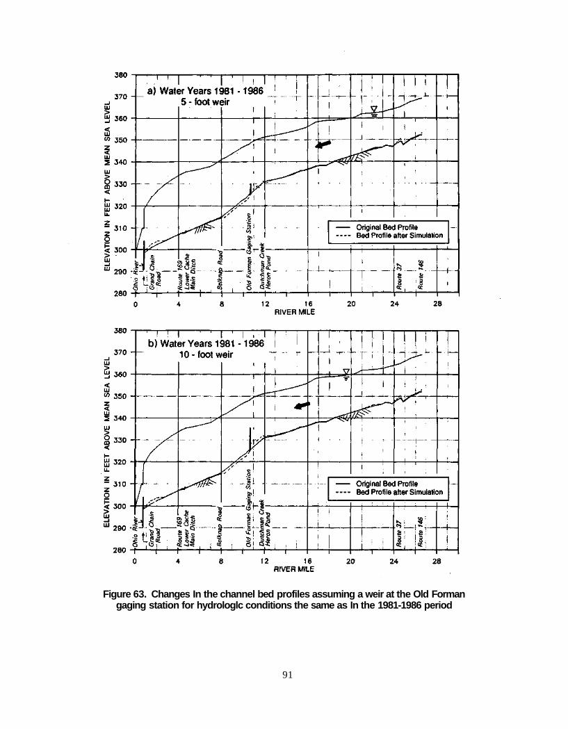
Figure 63. Changes In the channel bed profiles assuming a weir at the Old Forman gaging station for hydrologlc conditions the same as In the 1981-1986 period

91

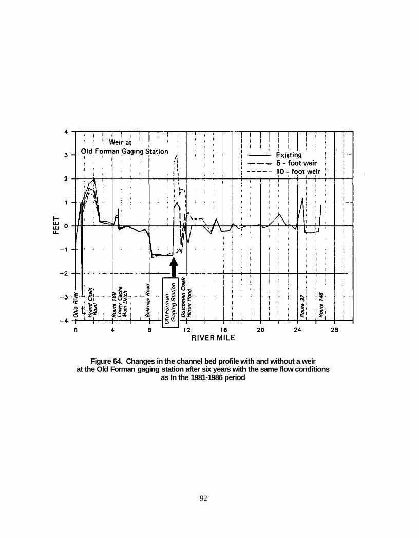
Figure 64. Changes in the channel bed profile with and without a weir at the Old Forman gaging station after six years with the same flow conditions

as In the 1981-1986 period

92

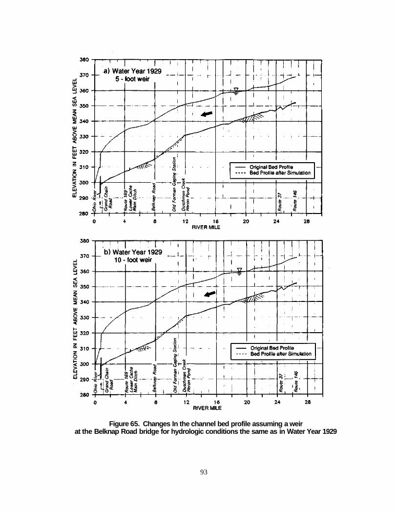
Figure 65. Changes In the channel bed profile assuming a weir at the Belknap Road bridge for hydrologic conditions the same as in Water Year 1929

93

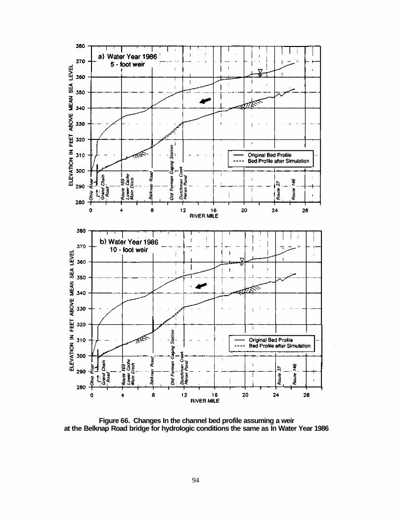
Figure 66. Changes In the channel bed profile assuming a weir at the Belknap Road bridge for hydrologic conditions the same as In Water Year 1986

94

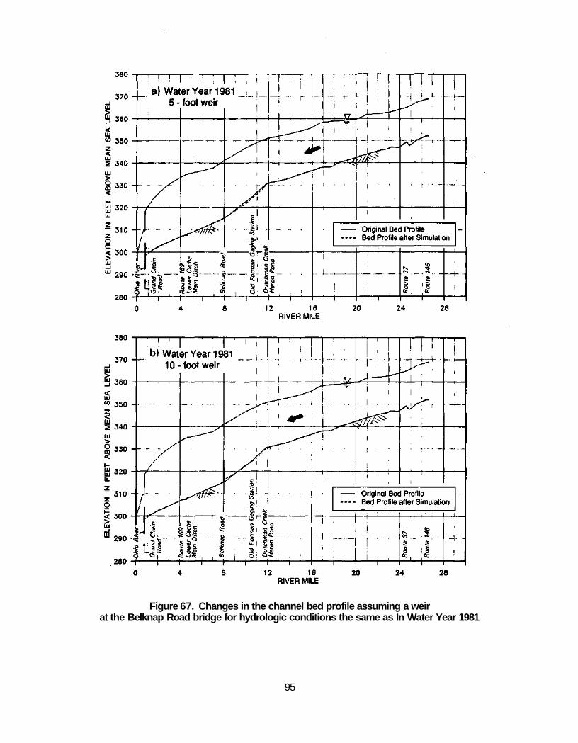
Figure 67. Changes in the channel bed profile assuming a weir at the Belknap Road bridge for hydrologic conditions the same as In Water Year 1981

95

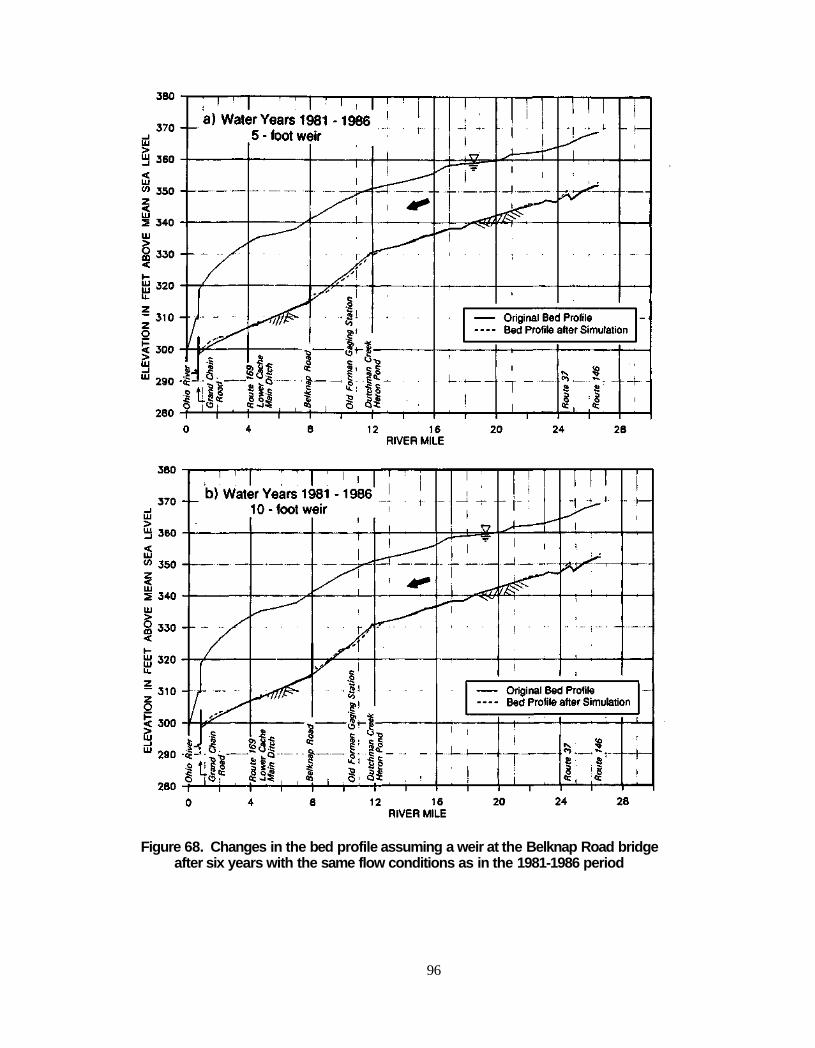
Figure 68. Changes in the bed profile assuming a weir at the Belknap Road bridge after six years with the same flow conditions as in the 1981-1986 period

96

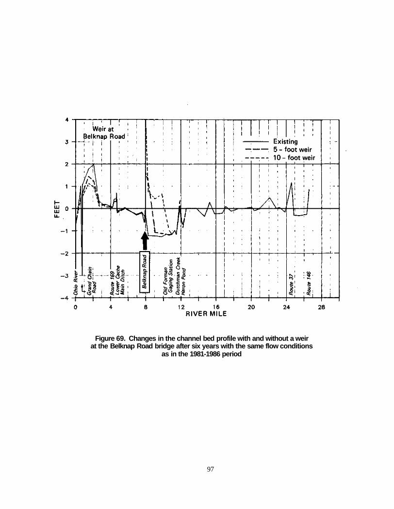
Figure 69. Changes in the channel bed profile with and without a weir at the Belknap Road bridge after six years with the same flow conditions

as in the 1981-1986 period

97

SUMMARY This report summarizes the use of mathematical models in an investigation of the

hydraulics and hydrology of the Cache River basin. Two different models were used in the study. The HEC-1 model was used to investigate flooding in the Lower Cache River, and the HEC-6 model was used to investigate flood elevations and sediment transport as they relate to channel entrenchment in the Upper Cache River.

The problems in the Lower and Upper Cache Rivers are different. In the Lower Cache River, the main problems are flooding and sedimentation. Because of the flooding problems, the local drainage district has been attempting to clear the Cache River channel and floodplain. Such operations, if permitted without an environmental impact assessment, could destroy the natural areas and wetlands in the Lower Cache River Natural Area (LCRNA). The sedimentation problem is associated with an increased sediment load in the tributary streams that drain into the LCRNA and with the inability of the Lower Cache River to transport the incoming sediment out of the LCRNA. The sedimentation problem in the Lower Cache River was not investigated by using models but is being analyzed on the basis of sediment input and output measurements and sedimentation rates.

The purpose of using the HEC-1 in the Lower Cache River was to investigate flooding conditions in the LCRNA under different precipitation and control measures. The HEC-1 model was calibrated by using data collected for Big and Cypress Creeks, which are the major tributaries of the Lower Cache River in the LCRNA, and by transferring parameter values to ungaged areas. Further calibrations and verifications were performed for the whole area by using flow and stage records at Route 51, which is the main outlet of flow from the LCRNA, and at several locations within the LCRNA. After the calibrations and verifications were completed, the HEC-1 was used to generate runoff from tributary streams, to route the water through the LCRNA, and to determine flood elevations in the LCRNA. It is now possible to use the HEC-1 model to investigate the impacts of different alternatives on flood elevations in the LCRNA.

The problem in the Upper Cache River is different from that in the Lower Cache River. The main problem is channel entrenchment along the Upper Cache River, and its impacts on the hydrology of wetlands in the area. Even though this has not been a major problem since the construction of the Forman Floodway levee, the influence of the Ohio River on flood elevations along this stretch of the river is an important consideration. The HEC-6 was used to investigate the influence of the Ohio River on flood stages along Post Creek and the Upper Cache River. The HEC-6 was calibrated by using stage records for the Cache River at Forman and at Route 146. Sediment inflow information for the main river and tributary streams was obtained from the sediment monitoring data collected by the ISWS at three locations in the study area. Bed material characteristics were determined from data collected by the ISWS for this project.

98

The HEC-6 results show that the Ohio River stages influence flood stages in the Post Creek Cutoff and the Upper Cache River all the way upstream past the Cache River levee to the Heron Pond area. The influence of the Ohio River is more pronounced for more frequent floods than for less frequent floods. It is important to consider the impacts that the Ohio River floods might have on the Lower and Upper Cache before implementing any changes in the present system. Of special concern will be any modifications along the Cache River levee.

Sediment transport analysis was carried out for different hydrologic conditions, since the nature of sediment transport depends on the hydrologic conditions. Four different hydrologic conditions (one high-flow year, one average-flow year, one low-flow year, and a six-year period for long-term analysis) were used as input data. The results of the sediment transport analysis showed that the Upper Cache River has not reached stable channel conditions. Channel scour is taking place at several locations along the Upper Cache River. The greatest amount of channel scour is taking place in a segment of the river with the highest slope from the Belknap Road bridge to Heron Pond. A rock outcrop in the Heron Pond area is preventing an upstream migration of the channel scour. How stable the rock bottom will remain, and for how long it will remain stable, are unknown.

Model simulations were also run to investigate how weir structures would influence channel scour. Weir structures at two locations, the Old Forman gaging station and the Belknap Road bridge, were investigated as to their effectiveness in reducing or terminating channel scour. The weir structures were assumed to have heights of either 5 or 10 feet. In general, it was found that sediment accumulation and channel aggradation will occur upstream of the weir structures. The erosion and sedimentation pattern downstream of the structures will not change significantly. The 10-foot weirs result in higher sediment accumulation and channel aggradation than the 5-foot weirs. The Old Forman gaging station site was found to prevent channel scour and to cause some channel aggradation between the structure and Heron Pond. The Belknap Road site reduces channel scour and creates some channel aggradation upstream of the site, but will not terminate channel scour in the area just downstream of Heron Pond. Therefore, if only one weir structure is to be constructed, it has to be located between the Old Forman gaging station site and Heron Pond.

The two models that have been developed for the Lower and Upper Cache Rivers perform their intended purposes very well. They are intended to be used for evaluating alternative solutions in the Cache River basin so that informed decisions can be made about the future of this important resource.

99

REFERENCES

Barnes, H.H. 1967. Roughness Characteristics of Natural Channels. U.S. Geological Survey Water Supply Paper 1849.

Chow, V.T. 1959. Open Channel Hydraulics. McGraw-Hill, New York, New York.

Chow, V.T. 1964. Statistical and Probability Analysis of Hydrologic Data. In Handbook of Applied Hydrology, edited by V.T. Chow, McGraw-Hill, New York, New York.

Clark, CO. 1945. Storage and the Unit Hydrograph. Transactions. American Society of Civil Engineers, Vol. 110, pp. 1419-1488.

Crawford, N.H., and Linsley, R.K. 1966. Digital Simulation in Hydrology: Stanford Watershed Model IV. Stanford University, Department of Civil Engineering Technical Report 39.

Demissie, M., W.C. Bogner, V. Tsihrintzis, and N.G. Bhowmik. 1986. Channel Scour Induced by Spillway at Lake Charleston, Illinois. Illinois State Water Survey Contract Report 409, Champaign, Illinois.

Demissie, M., V. Tsihrintzis, W.C. Bogner, and N.G. Bhowmik. 1988. Channel Scour Induced by Spillway Failure at Lake Charleston, Illinois. Journal of Hydraulic Engineering, American Society of Civil Engineers, Vol. 114, No. 8, 32 pp. 844-860.

Demissie, M., and B. Stephanatos. 1985. Computer Modeling of Lake Sedimentation. Proceedings of the Illinois Conference on Lake and Watershed Management, Water Resources Center, University of Illinois at Urbana-Champaign, Special Report 15, pp. 119-127.

Ford, D.T., E.C. Morris, and A.D. Feldman. 1980. Corps of Engineers' Experience with Automatic Calibration of Precipitation-Runoff Model. In Water and Related Land Resources Systems, edited by Y. Haimes and J . Kindler, Pergamon Press, New York, New York.

Garde, R.J., and K.G. Ranga Raju. 1985. Mechanics of Sediment Transportation and Alluvial Stream Problems. Halsted Press, John Wiley & Sons, Inc., New York.

Graf. W.H. 1971. Hydraulics of Sediment Transport. McGraw-Hill, New York, New York.

Holton, H.N., G.J. Stitner, W.H. Henson, and N.C. Lopez. 1975. USDAHL-74 Revised Model of Watershed Hydrology. Technical Bulletin 1518, Agricultural Research Service, U.S. Department of Agriculture, Washington, D.C.

Laursen, E.M. 1958. The Total Sediment Load of Streams. Journal of the Hydraulics Division. American Society of Civil Engineers, Vol. 84, No. HY1, pp. 1530-1 -1530-36.

Melching, C.S. 1987. A Reliability Analysis on Flood Event Forecasting with Uncertainties. Ph.D. Thesis, Department of Civil Engineering, University of Illinois at Urbana-Champaign.

Nash, J.E., and J.V. Sutcliffe. 1971. River Flow Forecasting through Conceptual Models, Part I - A Discussion of Principles. Journal of Hydrology. Vol. 10, No. 3, pp. 282-290.

100

Sherman, L.K. 1932. Stream Flow from Rainfall by the Unit-Graph Method. Engineering News-Record. Vol. 108, pp. 501-505.

Simons, D.B., and F. Senturk. 1977. Sediment Transport Technology. Water Resources Publications, Fort Collins, Colorado.

Soil Conservation Service (SCS). 1969. Unpublished cross-sectional survey data. Champaign, Illinois.

Soil Conservation Service (SCS). 1972. Unpublished cross-sectional survey data. Champaign, Illinois.

Toffaleti, F.B. 1966. A Procedure for Computation of Total River Sand Discharge and Detailed Distribution, Bed to Surface. Committee on Channel Stabilization, U.S. Army Corps of Engineers.

U.S. Geological Survey. Various years. Water Resources Data, Illinois. U.S. Geological Survey Water Data Report, Department of the Interior.

U.S. Army Corps of Engineers (USACOE). 1977. HEC-6, Scour and Deposition in Rivers and Reservoirs, User's Manual. The Hydrologic Engineering Center, Davis, California.

U.S. Army Corps of Engineers (USACOE). 1982. HEC-2, Water Surface Profiles. The Hydrologic Engineering Center, Davis, California.

U.S. Army Corps of Engineers (USACOE). 1987. HEC-1 Flood Hydrograph Package-User's Manual. U.S. Corps of Engineers Hydrologic Engineering Center, Computer Program No. 723-010.

Vanoni, V.A. 1977. Sedimentation Engineering. American Society of Civil Engineers, New York, New York.

Woolhiser, D.A. 1975. Simulation of Unsteady Overland Flow. In Unsteady Flow in Open Channels, edited by K. Mahmood and V. Yevjevich, Water Resources Publications, Colorado.

Yang, C.T. 1976. Minimum Unit Stream Power and Fluvial Hydraulics. Journal of the Hydraulics Division. Proceedings, ASCE, Vol. 102, No. HY7, Paper 12238, pp. 919-934.

101