An Introduction to Core-conductor Theory

“I often say when you can measure what you are speaking about

and express it in numbers you know something about it; but when

you cannot measure it, when you cannot express it in numbers, your

knowledge of it is of a meagre and unsatisfactory kind.”

Lord Kelvin

1 Introduction

It would not be inaccurate to suggest that the manner in which electric currentflows along a semi-insulated conductor forms a central conceptual core in the-oretical neuroscience. The passive properties of dendrites and the propagatingaction potential are only explicable within the context of the cable equation.

The cable equation is a second order in space, first order in time, partial differ-ential equation 1. A form of this equation was probably first derived by WilliamThomson (1824-1907), later Lord Kelvin, during his involvement with the laying,design and analysis of the first trans-atlantic telegraph cables beginning in 1854.

The cable equation is based on the simple notion of transverse current leakagebetween an inner and outer conductor due to an imperfect insulator as a conse-quence of the longitudinal flow of current within the inner conductor.

2 Assumptions

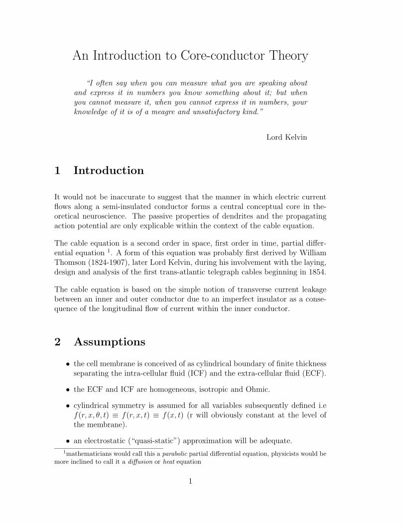
• the cell membrane is conceived of as cylindrical boundary of finite thicknessseparating the intra-cellular fluid (ICF) and the extra-cellular fluid (ECF).

• the ECF and ICF are homogeneous, isotropic and Ohmic.

• cylindrical symmetry is assumed for all variables subsequently defined i.ef(r, x, θ, t) ≡ f(r, x, t) ≡ f(x, t) (r will obviously constant at the level ofthe membrane).

• an electrostatic (“quasi-static”) approximation will be adequate.

1mathematicians would call this a parabolic partial differential equation, physicists would bemore inclined to call it a diffusion or heat equation

1

• currents in the inner and outer conductors will flow in the longitudinal (x)direction only.

• trans-membrane current flows in the radial (r) direction only

inner conductor

insulator (membrane)

outer conductora

Figure 1: Cross-section of the model cable illustrating the geometry of the innerconductor, insulator and outer conductor.

3 Definitions

• Io(x, t) = the total longitudinal current flowing in the +x direction in theouter conductor. (A)

• Ii(x, t) = the total longitudinal current flowing in the +x direction in theinner conductor. (A)

• Jm(x, t) is the membrane current density flowing from inner conductor to

outer conductor. (Am−2)

• Km(x, t) is the membrane current per unit length flowing from inner con-ductor to outer conductor. (Am−1) 2

• Keo(x, t) is the current per unit length due to external sources applied in acylindrically symmetric manner to the outer conductor. (Am−1)

• Kei(x, t) is the current per unit length applied to the inner conductor.(Am−1)

2this is the neurophysiological or physiologists convention and is often referred to as the“inward negative” definition in that the trans-membrane current is defined as negative when itflows from outer conductor to inner conductor. We will return to the issue of conventions atthe end of this chapter.

2

• Vi(x, t) is the potential of the inner conductor. (V )

• Vo(x, t) is the potential of the outer conductor. (V )

• Vm(x, t) = Vi(x, t) − Vo(x, t) is the trans-insulator (i.e trans-membrane)potential. (V )

• ri is the resistance per unit length of the inner, cylindrically symmetricconductor. (Ωm−1)

• ro is the resistance per unit length of the outer, cylindrically symmetricconductor. (Ωm−1)

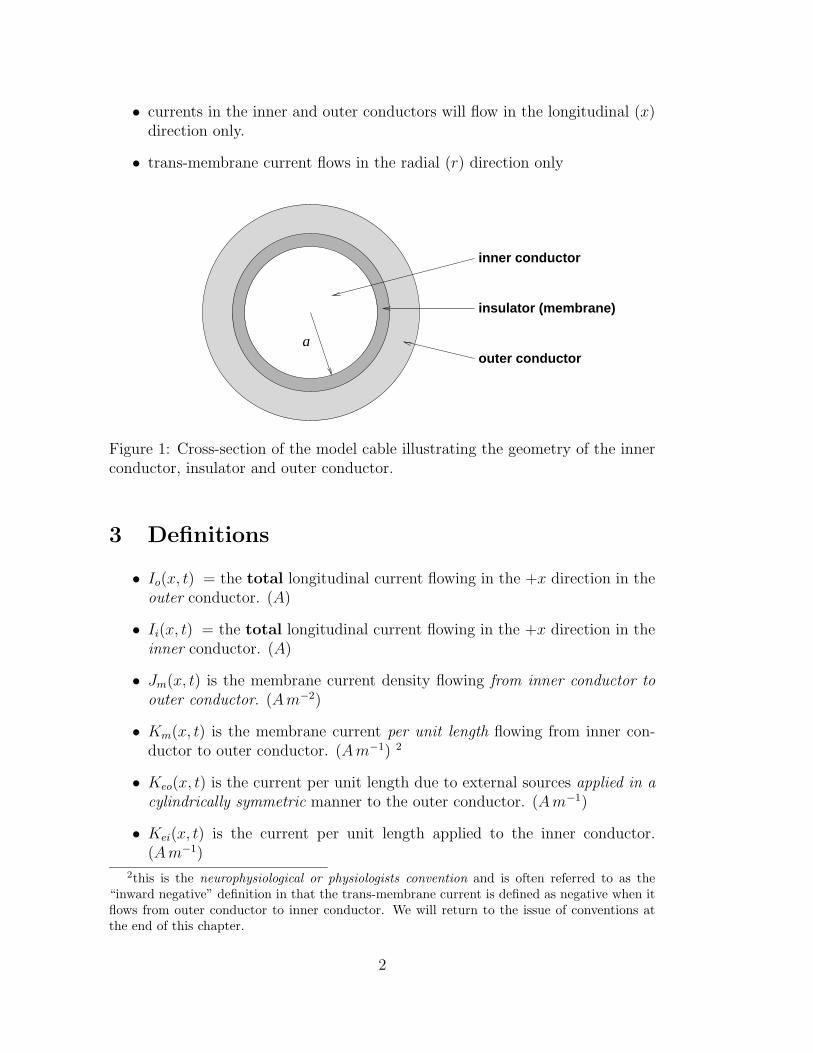
• a is the internal radius of the cylindrical shell. (m)

PSfrag replacements a

ri∆x

∆x

Figure 2: Geometry of the inner conductor

Based on these definitions and assumptions we are now able to represent conciselyin diagrammatic form the structure of the cable. This is illustrated in Figure 3.Note that we have “collapsed” the cylindrical symmetry of the cable.

4 Derivation of the core-conductor equations

While it is quite easy to derive the cable equation directly without noting anyintermediate equations it is more profitable to derive a limited form of the cableequation, called the core-conductor equations, which require no assumptions bemade about the structure of the cell membrane or insulator. The core-conductorequations are easily derived by the use of Kirchoff’s electrical circuit laws and aspatially discrete cable.

3

(x,t)

ri ∆x ri ∆x

r ∆xo r ∆xo r ∆xo

∆x(x+ ,t)ViVi(x,t)ri ∆x

(x,t)Km ∆x

∆x(x,t)eiK ∆x∆x(x+ ,t)eiK

∆x(x,t)eoK

i(x,t)I ∆x(x+ ,t)iI

∆x(x+ ,t)Km ∆x

∆x x+

∆x

∆x∆x(x+ ,t)

∆x

oI

Vo

K eo

Vo

oI

(a) (b)

(c) (d)

outer conductor

inner conductor

insulator (membrane)

x

(x,t) (x+ ,t)

(x+ ,t)

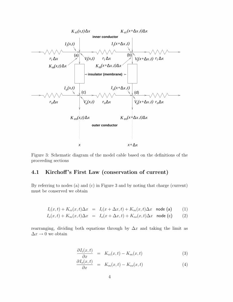
Figure 3: Schematic diagram of the model cable based on the definitions of theproceeding sections

4.1 Kirchoff’s First Law (conservation of current)

By referring to nodes (a) and (c) in Figure 3 and by noting that charge (current)must be conserved we obtain

Ii(x, t) +Kei(x, t)∆x = Ii(x+∆x, t) +Km(x, t)∆x node (a) (1)

Io(x, t) +Km(x, t)∆x = Io(x+∆x, t) +Keo(x, t)∆x node (c) (2)

rearranging, dividing both equations through by ∆x and taking the limit as∆x→ 0 we obtain

∂Ii(x, t)

∂x= Kei(x, t)−Km(x, t) (3)

∂Io(x, t)

∂x= Km(x, t)−Keo(x, t) (4)

4

4.2 Kirchoff’s Second Law (conservation of energy)

From Figure 3 and a simple application of Ohm’s Law we obtain

Vi(x, t)− Vi(x+∆x, t) = ri∆xIi(x+∆x, t) nodes (a) and (b) (5)

Vo(x, t)− Vo(x+∆x, t) = ro∆xIo(x+∆x, t) nodes (c) and (d) (6)

dividing through by ∆x and taking the limit as ∆x→ 0 we obtain

∂Vi(x, t)

∂x= −riIi(x, t) (7)

∂Vo(x, t)

∂x= −roIo(x, t) (8)

However Vm = Vi − Vo and thus by subtracting equation (8) from (7) we obtain

∂Vm(x, t)

∂x= roIo(x, t)− riIi(x, t) (9)

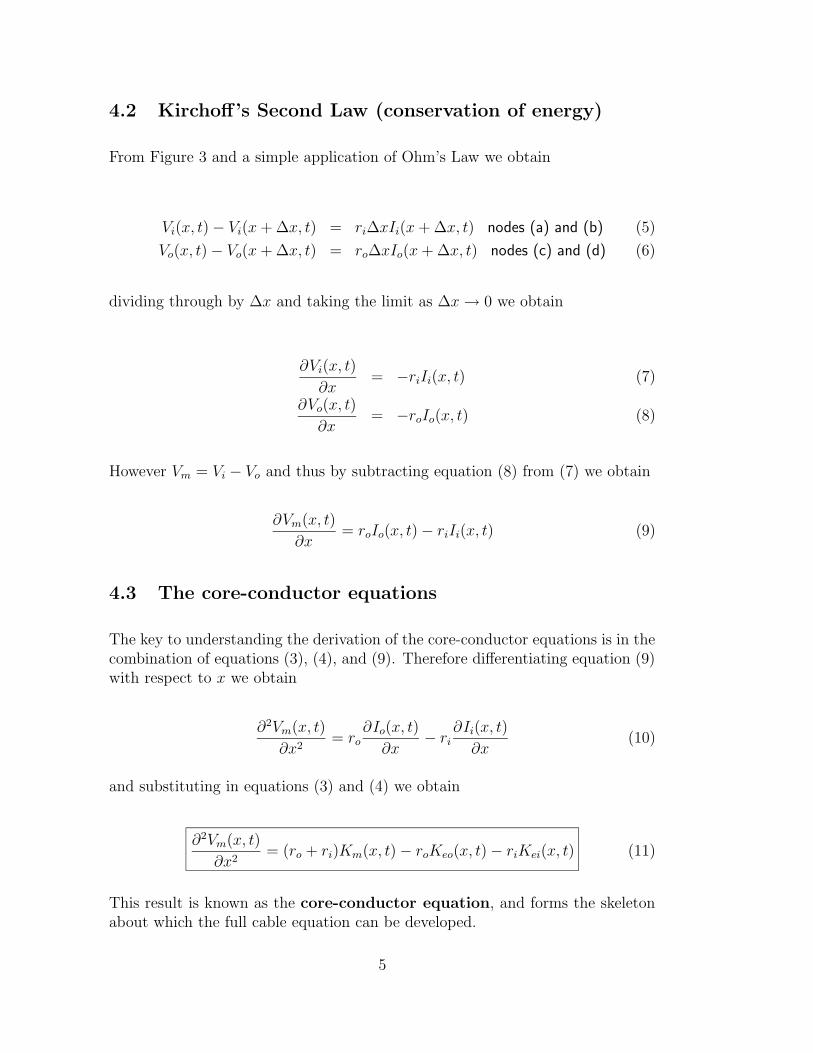
4.3 The core-conductor equations

The key to understanding the derivation of the core-conductor equations is in thecombination of equations (3), (4), and (9). Therefore differentiating equation (9)with respect to x we obtain

∂2Vm(x, t)

∂x2= ro

∂Io(x, t)

∂x− ri

∂Ii(x, t)

∂x(10)

and substituting in equations (3) and (4) we obtain

∂2Vm(x, t)

∂x2= (ro + ri)Km(x, t)− roKeo(x, t)− riKei(x, t) (11)

This result is known as the core-conductor equation, and forms the skeletonabout which the full cable equation can be developed.

5

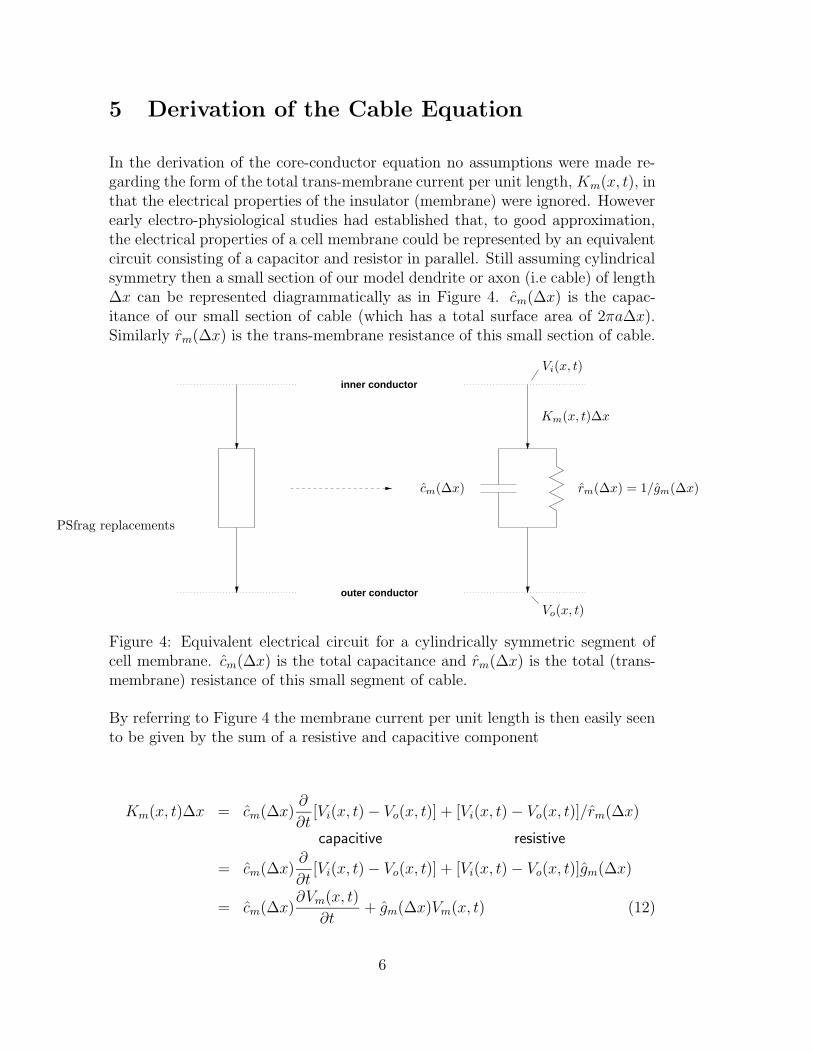
5 Derivation of the Cable Equation

In the derivation of the core-conductor equation no assumptions were made re-garding the form of the total trans-membrane current per unit length, Km(x, t), inthat the electrical properties of the insulator (membrane) were ignored. Howeverearly electro-physiological studies had established that, to good approximation,the electrical properties of a cell membrane could be represented by an equivalentcircuit consisting of a capacitor and resistor in parallel. Still assuming cylindricalsymmetry then a small section of our model dendrite or axon (i.e cable) of length∆x can be represented diagrammatically as in Figure 4. cm(∆x) is the capac-itance of our small section of cable (which has a total surface area of 2πa∆x).Similarly rm(∆x) is the trans-membrane resistance of this small section of cable.

outer conductor

inner conductor

PSfrag replacements

Vi(x, t)

Vo(x, t)

cm(∆x) rm(∆x) = 1/gm(∆x)

Km(x, t)∆x

Figure 4: Equivalent electrical circuit for a cylindrically symmetric segment ofcell membrane. cm(∆x) is the total capacitance and rm(∆x) is the total (trans-membrane) resistance of this small segment of cable.

By referring to Figure 4 the membrane current per unit length is then easily seento be given by the sum of a resistive and capacitive component

Km(x, t)∆x = cm(∆x)∂

∂t[Vi(x, t)− Vo(x, t)] + [Vi(x, t)− Vo(x, t)]/rm(∆x)

capacitive resistive

= cm(∆x)∂

∂t[Vi(x, t)− Vo(x, t)] + [Vi(x, t)− Vo(x, t)]gm(∆x)

= cm(∆x)∂Vm(x, t)

∂t+ gm(∆x)Vm(x, t) (12)

6

As defined the membrane capacitance and membrane resistance are functions of∆x. In order to take the limit as ∆x → 0 a more explicit relationship betweenthese quantities and ∆x is required. Therefore assuming that cm(∆x) and rm(∆x)are not functions of x we can define the the following relationships

cm(∆x) = cm∆x = 2πaCm∆x (13)

gm(∆x) = gm∆x = 2πaGm∆x (14)

where cm and gm are the capacitance and conductance per unit length respectively(F m−1, S m−1) and Cm and Gm are the capacitance and conductance per unitarea respectively (F m−2, S m−2). By inserting these definitions into equation(12) and dividing both sides through by ∆x we obtain

Km(x, t) = cm

∂Vm(x, t)

∂t+ Vmgm (15)

= cm

∂Vm(x, t)

∂t+ Vm/rm (16)

Be careful to note the meaning and units of rm in the last equation ! By substitut-ing equation (16) into (11) and rearranging we obtain the following second-orderpartial differential equation

rmcm

∂Vm

∂t=

rm

ro + ri

∂2Vm

∂x2+ roKeo(x, t) + riKei(x, t)

− Vm (17)

This result is commonly referred to as the cable equation. Ignoring any externalcurrent input (i.e Kei = Keo = 0) it is often convenient to rewrite the aboveequation as

τm

∂Vm

∂t= λ2

c

∂2Vm

∂x2− Vm (18)

where λc =√

rm/(ro + ri) and τm = rmcm3. For reasons that will soon become

apparent λc is called the cable space constant and τm is called the membrane timeconstant. Further by defining the dimensionless quantities X = x/λc and T =

3the student should note that rmcm = RmCm, where Rm = 1/Gm

7

t/τm equation (18) can be written as the following parabolic partial differentialequation

∂Vm

∂T=

∂2Vm

∂X2− Vm (19)

Solutions of the partial differential equations so defined depend, in addition tothe stated electrical properties, on the initial conditions and the boundary con-ditions (i.e the value of Vm at either ends of the cable). Further, under certainassumptions, equations (17-19) are able to describe the passive properties of mul-tiply branched and tapered cables. The ability to incorporate multiply branchedcables is of particular interest in describing the passive electrical properties ofdendrites and axons. The interested reader should consult Rall (1989) for furtherdetails.

5.1 The cable space constant

Let a constant trans-membrane current be applied at some point along the modelcable. As the membrane capacitance becomes polarised with the passage of timethe trans-membrane current density will become a function of axial distance only.Thus for sufficiently long times ∂Vm

∂t→ 0. This corresponds to a steady state.

For increasing distances away from this site of current injection the membranepotential would be expected to decrease due to the continual trans-membraneleakage of current. Thus at steady state the partial differential cable equation isreduced to an ordinary differential equation (ODE)

λ2c

d2Vm

dx2= Vm (20)

As can be verified by direct substitution, a general solution to this ODE forconstant current applied at x = 0 is 4

Vm(x) = A exp[x/λc] +B exp[−x/λc] (21)

where A and B will depend on the boundary conditions. For boundary-value

4This is easily derived by substituting exp[−λx] into the differential equation. The solution ofthe resulting characteristic equation (which is a simple quadratic equation) defines the solutionbasis set. The student should refer to any textbook on the solution of ordinary differentialequations to be reminded of the procedure.

8

solutions it is often convenient to use another pair of solutions to the second-orderordinary differential equation which are (as can be verified by direct substitution)

Vm(x) = A cosh(x/λc) +B sinh(x/λc) (22)

where cosh(x) = (exp[x] + exp[−x])/2 and sinh(x) = (exp[x]− exp[−x])/2.

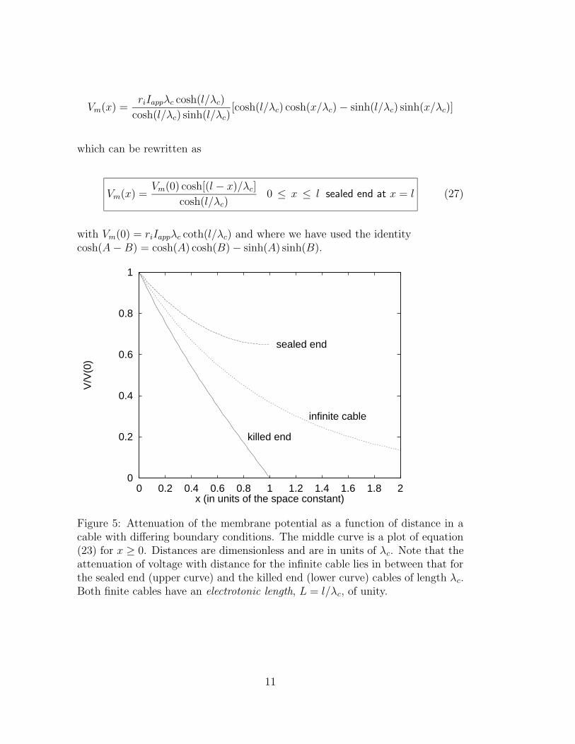
The space constant is useful as a parameter for estimating how far an axon ordendrite can propagate activity passively. Typical values for large myelinatedaxons are 1 − 2 mm whereas for small unmyelinated axons or dendrites thevalues range upwards from 30 µm. We will now consider the determination ofthe coefficients for the following three cases

• infinite cylinder

• a finite cylinder of length l with a sealed ends at x = 0 and x = l

• a finite cylinder of length l with a sealed end at x = 0 and a killed end atx = l (i.e the end at x = l is clamped to the resting membrane potentialVm = 0)

5.1.1 infinite cylinder

For the case in which the cable extends from −∞ to +∞ we require

V (−∞) = V (∞) = 0

and thus for x ≥ 0 A = 0 and B = V0 in equation (21), where V0 is the membranepotential at the site of the current passing electrode. Similarly for x ≤ 0 A = V0

and B = 0 and thus

Vm(x) = V0 exp[−|x|/λc] (23)

for a constant current applied at x = 0.

9

5.1.2 finite cylinder, sealed end at x = l

The idea of the sealed end is that axial current is prevented from flowing acrossa boundary. For the case now considered this boundary will be the end of thecable at x = l. Further we will assume that a current, Iapp, is injected at x = 0at the inner conductor and Vm has attained its steady-state value. By referringto equation (9) it is seen that the following conditions must be satisfied

dVm

dx

∣

∣

∣

∣

x=0

= −riIapp

dVm

dx

∣

∣

∣

∣

x=l

= 0 (24)

These conditions are known as Neumann conditions 5. These boundary conditionsare used to solve for the coefficients A and B in our general solution (22) byobserving that

dVm

dx=

A

λc

sinh(x/λc) +B

λc

cosh(x/λc) (25)

Thus at x = 0 −riIapp = B/λc i.e B = −riIappλc, whereas at x = l

0 = A sinh(l/λc) +B cosh(l/λc)

which gives

A = −B coth(l/λc)

= riIappλc coth(l/λc)

where coth(x) = cosh(x)/ sinh(x). Thus the solution is

Vm(x) = riIappλc[coth(l/λc) cosh(x/λc)− sinh(x/λc)] (26)

by rearranging the above equation we get

5More specifically Neumann conditions specify normal gradients on the boundary.

10

Vm(x) =riIappλc cosh(l/λc)

cosh(l/λc) sinh(l/λc)[cosh(l/λc) cosh(x/λc)− sinh(l/λc) sinh(x/λc)]

which can be rewritten as

Vm(x) =Vm(0) cosh[(l − x)/λc]

cosh(l/λc)0 ≤ x ≤ l sealed end at x = l (27)

with Vm(0) = riIappλc coth(l/λc) and where we have used the identitycosh(A−B) = cosh(A) cosh(B)− sinh(A) sinh(B).

0

0.2

0.4

0.6

0.8

1

0 0.2 0.4 0.6 0.8 1 1.2 1.4 1.6 1.8 2

V/V

(0)

x (in units of the space constant)

killed end

infinite cable

sealed end

Figure 5: Attenuation of the membrane potential as a function of distance in acable with differing boundary conditions. The middle curve is a plot of equation(23) for x ≥ 0. Distances are dimensionless and are in units of λc. Note that theattenuation of voltage with distance for the infinite cable lies in between that forthe sealed end (upper curve) and the killed end (lower curve) cables of length λc.Both finite cables have an electrotonic length, L = l/λc, of unity.

11

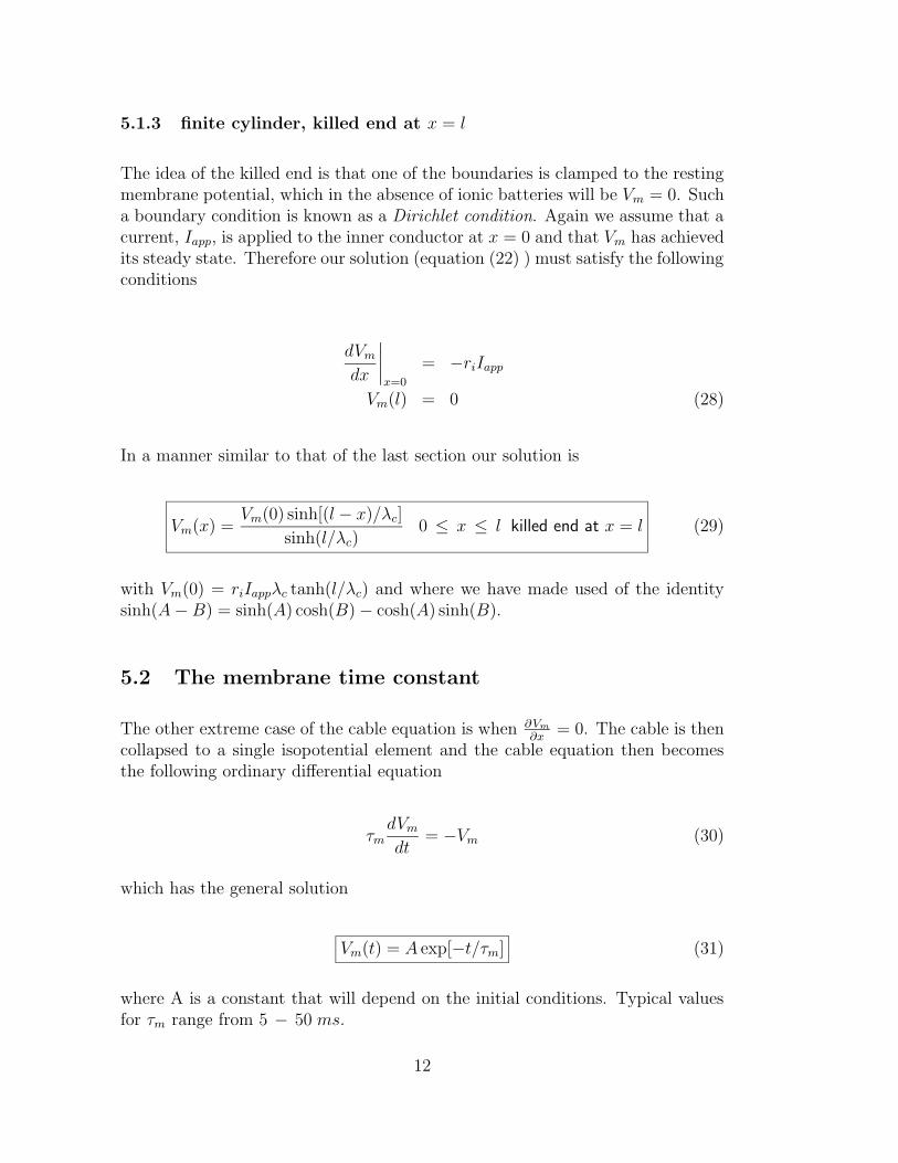
5.1.3 finite cylinder, killed end at x = l

The idea of the killed end is that one of the boundaries is clamped to the restingmembrane potential, which in the absence of ionic batteries will be Vm = 0. Sucha boundary condition is known as a Dirichlet condition. Again we assume that acurrent, Iapp, is applied to the inner conductor at x = 0 and that Vm has achievedits steady state. Therefore our solution (equation (22) ) must satisfy the followingconditions

dVm

dx

∣

∣

∣

∣

x=0

= −riIapp

Vm(l) = 0 (28)

In a manner similar to that of the last section our solution is

Vm(x) =Vm(0) sinh[(l − x)/λc]

sinh(l/λc)0 ≤ x ≤ l killed end at x = l (29)

with Vm(0) = riIappλc tanh(l/λc) and where we have made used of the identitysinh(A−B) = sinh(A) cosh(B)− cosh(A) sinh(B).

5.2 The membrane time constant

The other extreme case of the cable equation is when ∂Vm

∂x= 0. The cable is then

collapsed to a single isopotential element and the cable equation then becomesthe following ordinary differential equation

τm

dVm

dt= −Vm (30)

which has the general solution

Vm(t) = A exp[−t/τm] (31)

where A is a constant that will depend on the initial conditions. Typical valuesfor τm range from 5 − 50 ms.

12

5.3 The addition of ionic batteries

Trans-membrane current is mediated by the flux of ions, through protein pores,between the intra-cellular and extra-cellular fluids. The flux of each type ofion will depend on its electro-chemical gradient, which in turn depends on thetrans-membrane concentration gradients and the cell membrane potential, andthe selective permeability of the membrane to any given ionic species. Further,the membrane permeability for any given ion may be regulated by one or moreconductances. All of these conductances may be regulated by endogenous ligands(e.g neurotransmitters), membrane potential and the concentrations of other ionsin the extracellular and intracellular fluids. The total trans-membrane currentdensity will depend on the contributions of the individual ionic currents. Figure 6displays a circuit diagram describing the electrical properties of nerve membranewhich incorporates the individual ionic currents.

extracellular

intracellular

PSfrag replacements

Ei Ej Ek

Gi(x, t) Gj(x, t) Gk(x, t)

Ji(x, t) Jj(x, t) Jk(x, t)Jc(x, t)

Jm(x, t)

Cm

Figure 6: An equivalent electrical circuit of a small section of neuron membrane.See text for definitions.

From Figure 6 it is easily ascertained that

Jm = Jc +∑

k

Jk (32)

where Jm is the total trans-membrane current flowing per unit area (Am−2) whichis composed of a capacitive current (Jc = Cm

∂Vm

∂t) and k ionic currents (Jk). For

each ionic conductance we have

13

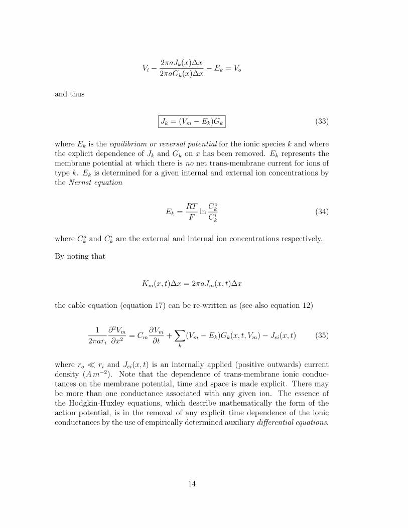
Vi −2πaJk(x)∆x

2πaGk(x)∆x− Ek = Vo

and thus

Jk = (Vm − Ek)Gk (33)

where Ek is the equilibrium or reversal potential for the ionic species k and wherethe explicit dependence of Jk and Gk on x has been removed. Ek represents themembrane potential at which there is no net trans-membrane current for ions oftype k. Ek is determined for a given internal and external ion concentrations bythe Nernst equation

Ek =RT

Fln

Cok

C ik

(34)

where Cok and C i

k are the external and internal ion concentrations respectively.

By noting that

Km(x, t)∆x = 2πaJm(x, t)∆x

the cable equation (equation 17) can be re-written as (see also equation 12)

1

2πari

∂2Vm

∂x2= Cm

∂Vm

∂t+∑

k

(Vm − Ek)Gk(x, t, Vm)− Jei(x, t) (35)

where ro ¿ ri and Jei(x, t) is an internally applied (positive outwards) currentdensity (Am−2). Note that the dependence of trans-membrane ionic conduc-tances on the membrane potential, time and space is made explicit. There maybe more than one conductance associated with any given ion. The essence ofthe Hodgkin-Huxley equations, which describe mathematically the form of theaction potential, is in the removal of any explicit time dependence of the ionicconductances by the use of empirically determined auxiliary differential equations.

14

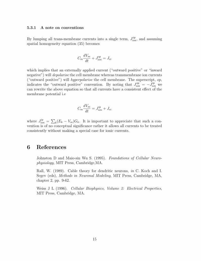
5.3.1 A note on conventions

By lumping all trans-membrane currents into a single term, J opion, and assuming

spatial homogeneity equation (35) becomes

Cm

dVm

dt+ Jop

ion = Jei

which implies that an externally applied current (“outward positive” or “inwardnegative”) will depolarise the cell membrane whereas transmembrane ion currents(“outward positive”) will hyperpolarise the cell membrane. The superscript, op,indicates the “outward positive” convention. By noting that J op

ion = −Jipion we

can rewrite the above equation so that all currents have a consistent effect of themembrane potential i.e

Cm

dVm

dt= J ip

ion + Jei

where J ipion =

∑

k(Ek − Vm)Gk. It is important to appreciate that such a con-vention is of no conceptual significance rather it allows all currents to be treatedconsistently without making a special case for ionic currents.

6 References

Johnston D and Maio-sin Wu S. (1995). Foundations of Cellular Neuro-

physiology, MIT Press, Cambridge,MA.

Rall, W. (1989). Cable theory for dendritic neurons, in C. Koch and I.Segev (eds), Methods in Neuronal Modeling, MIT Press, Cambridge, MA,chapter 2, pp. 9-62.

Weiss J L (1996). Cellular Biophysics, Volume 2: Electrical Properties,MIT Press, Cambridge, MA.

15