Chapter 6

C4 Stator Observations

6.1 Introduction

The performance of an embedded blade row in an axial turbomachine is largely dic-

tated by transitional flow phenomena occurring on the surface of blade row elements.

This process is known to be influenced by many factors including unsteady flow effects

which occur due to the relative motion between adjacent blade rows. As discussed

in Chapter 5, one common source of unsteady flow is vortical disturbances caused

by the relative motion of wakes convected from upstream blade rows. The disper-

sion and interaction of these wakes lead to pitchwise-periodic variations in time-mean

flow, periodic disturbance level and random turbulent fluctuations. Machines that

have identical blade numbers in adjacent rotor–stator blade row pairs can alter the

relative circumferential alignment to influence performance. This process, known as

‘indexing’ or blade row ‘clocking’, has been suggested by many researchers as a way

of improving efficiency and influencing noise generation.

It should also be noted that skewing of wakes due to radial variation in peripheral

velocity means that blade elements at different radial locations experience different

wake disturbance regimes. Average performance increase due to clocking will therefore

be less than the optimum for an individual blade element.

Blade row clocking effects have previously been studied using the UTAS research

compressor. Walker et al. [180] surveyed the stator inlet flow field with a hot-wire

probe using a similar approach to the investigation detailed in Chapter 5. Surveys

performed downstream from the stator blade row were used to determine tempo-

ral variations of stator wake momentum thickness. This procedure was repeated for

6.1 Introduction 82

several different IGV–stator blade row alignments. The study showed that wake mo-

mentum thickness varied by a greater amount for the clocking case where the IGV

wake street was aligned in the stator blade row passage. No firm conclusion could

be made with respect to the variation of time-mean stator wake momentum thick-

ness with clocking position, since the resulting differences were comparable with the

estimated level of uncertainty in the data.

Walker et al. [181] extended their earlier study to examine the effect of blade row

clocking on the unsteady boundary layer behaviour of a stator blade row element.

Measurements were made using an array of hot-film sensors mounted on the surface

of a stator blade. The study showed that clocking the IGV blade row relative to

the stator blade row caused significant changes in both the nature and extent of

boundary layer transition on the blade surface. The extent of periodic transitional

flow was greatly reduced in the case where the stator blade row was immersed in the

IGV wake street.

In another study, Mailach and Vogeler [110] investigated clocking effects in a four-

stage axial compressor. They found that the unsteady pressure fluctuations experi-

enced by a downstream stator were nearly independent of the convective wake distur-

bances; this was partially due to the low Mach number in the research compressor.

They also noted that the position of the upstream stator blade row greatly influenced

the magnitude of the unsteady pressure fluctuations.

Many other studies have focused on clocking effects in axial turbines. Hummel [86]

measured significant changes in shock strength with clocking position inside a tran-

sonic turbine cascade. Tiedemann and Kost [169] found that clocking a nozzle guide

vane blade row substantially influenced the magnitude of periodic pressure fluctua-

tions downstream from the turbine stator. These studies, and also those by Reinmoller

et al. [133], Haldeman et al. [58] and Jouini et al. [92], suggest that clocking may be

used to improve efficiency up to 1 percent. However, the current level of understand-

ing of the flow phenomena is not sufficient to allow firm conclusions to be made; in

some cases conflicting or inconclusive findings have been published.

The ability of single-stage machines to simulate the multi-stage environment has

previously been questioned in literature due to the lack of a high turbulence envi-

ronment characteristic of an embedded stage (see Place et al. [131]). This chapter

studies how free-stream turbulence and blade row clocking influence transitional flow

behaviour on a C4 stator blade in the UTAS research compressor. Measurements

6.2 Range of Investigation 83

using the natural low turbulence inflow configuration are compared to those at high

turbulence, the latter achieved using a turbulence grid at inlet. Surface hot-film

measurements show how boundary layer transition is altered by both free-stream tur-

bulence and IGV–stator blade row clocking. Significant conclusions are drawn about

the influence of free-stream turbulence on blade row clocking and the ability of 1.5-

stage machines to simulate the performance of an embedded blade row in a multi-stage

machine.

6.2 Range of Investigation

The measurements presented in this chapter were made using the same set of compres-

sor loading cases used in the study of the stator inlet flow field, described in Chapter 5.

These cases corresponded to high load (φ = 0.600), medium load (φ = 0.675) and low

load (φ = 0.840). The resulting stator surface pressure distributions were measured by

Solomon [154] using the long axial gap (LAG) configuration of the research compressor.

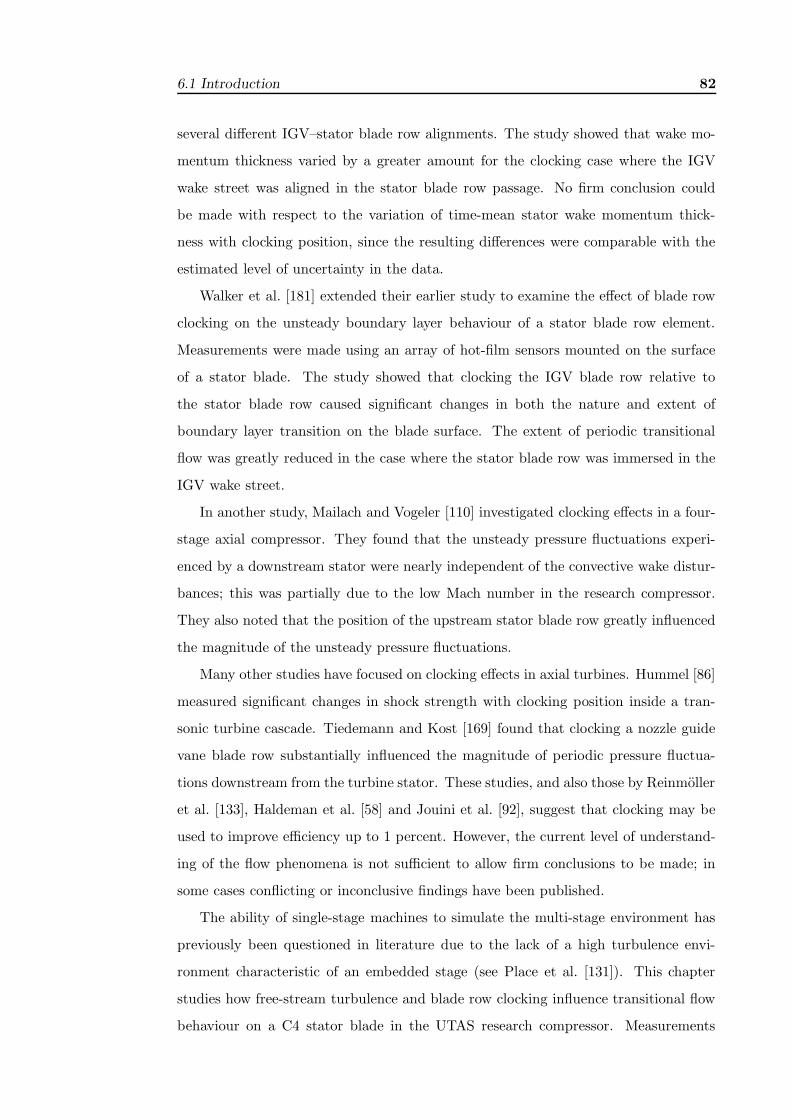
The resulting velocity distributions are shown in Fig. 6.1. A predicted surface velocity

distribution was obtained in the present study using the viscous/inviscid steady flow

solver MISES of Drela and Giles [36]. In this case the predicted velocity at the outer

edge of the boundary layer, U/U1 has been expressed as U/Umb using Eq. (4.3). The

inlet turbulence intensity was set to 1% for these simulations. No allowance was made

for changing axial velocity – density ratio.

The velocity distributions for both medium and high compressor loading show a

high level of similarity. The flow on the suction surface experiences a rapid acceleration

around the leading edge, reaching maximum velocity near s∗ = 0.05. This is followed

by a near linear deceleration over the remaining surface. The flow on the pressure

surface accelerates to maximum velocity at s∗ = 0.15. This is followed by a gentle

deceleration to s∗ = 0.7 and then a mild acceleration to the trailing edge.

The flow at low compressor loading is significantly different from the other cases.

Due to the negative incidence, the suction surface acceleration is more gradual with

maximum velocity occurring at approximately s∗ = 0.3. The presence of a large

mid-chord separation bubble is indicated by a discontinuity in pressure coefficient at

s∗ = 0.7. The flow on the pressure surface experiences a much stronger acceleration

and deceleration than in the other load cases.

The agreement between predicted and measured velocity distributions is generally

6.2 Range of Investigation 84

0.0 0.2 0.4 0.6 0.8 1.0s*

0.2

0.4

0.6

0.8

1.0

1.2

1.4

1.6

U/U

mb

0.840 -6.1 1300000.675 1.2 1170000.600 4.1 110000

LowMediumHigh

LOAD SS PS MISES i Re1

Figure 6.1: C4 stator surface velocity distribution at mid-span (Rec = 120000) forLAG configuration. Experimental data from Solomon [154]

good. At low loading (φ = 0.840) the suction surface separation bubble is predicted

close to the location observed in the experimental data. A separation bubble is also

predicted on the pressure surface near s∗ = 0.25. This is not indicated in the experi-

mental data: the hot-film measurements presented in Section 6.5 show that separation

occurs closer to the leading at 0.05 < s∗ < 0.1. Similarly, the suction surface separa-

tion bubbles predicted at s∗ = 0.35 in the high load case (φ = 0.600) and s∗ = 0.45 in

the medium load case (φ = 0.675) are not indicated in the experimental data. Strong

periodic transitional flow occurring on the surface, shown by the hot-film measure-

ments of Section 6.5, are likely for preventing separation bubbles that would normally

form at low turbulence in steady flow conditions.

At high loading (φ = 0.600), the agreement deteriorates toward the trailing edge.

This is likely due to changing axial velocity – density ratio that results from increas-

ingly non-uniform flow towards the hub as loading is increased.

The agreement between predicted and measured surface velocity distributions

demonstrates highly two-dimensional flow at mid-span position.

6.3 Time-Mean Stator Inlet Flow 85

6.3 Time-Mean Stator Inlet Flow

Three-hole probe surveys performed in the rotor–stator axial space were used to deter-

mine the time-mean distributions of total pressure and flow incidence. This provided

an important verification of changes resulting from installation of the turbulence grid.

Details of the probe and calibration are given in Section 3.4.8 and the measurement

procedure is outlined in Section 4.10.

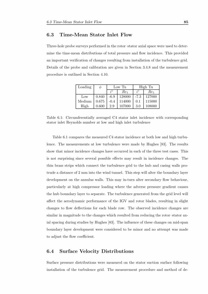
Loading φ Low Tu High Tui◦ Re1 i◦ Re1

Low 0.840 -6.9 128000 -7.3 127000Medium 0.675 -0.4 114000 0.1 115000

High 0.600 2.9 107000 3.0 108000

Table 6.1: Circumferentially averaged C4 stator inlet incidence with correspondingstator inlet Reynolds number at low and high inlet turbulence

Table 6.1 compares the measured C4 stator incidence at both low and high turbu-

lence. The measurements at low turbulence were made by Hughes [83]. The results

show that minor incidence changes have occurred in each of the three test cases. This

is not surprising since several possible effects may result in incidence changes. The

thin brass strips which connect the turbulence grid to the hub and casing walls pro-

trude a distance of 2 mm into the wind tunnel. This step will alter the boundary layer

development on the annulus walls. This may in-turn alter secondary flow behaviour,

particularly at high compressor loading where the adverse pressure gradient causes

the hub boundary layer to separate. The turbulence generated from the grid level will

affect the aerodynamic performance of the IGV and rotor blades, resulting in slight

changes to flow deflections for each blade row. The observed incidence changes are

similar in magnitude to the changes which resulted from reducing the rotor–stator ax-

ial spacing during studies by Hughes [83]. The influence of these changes on mid-span

boundary layer development were considered to be minor and no attempt was made

to adjust the flow coefficient.

6.4 Surface Velocity Distributions

Surface pressure distributions were measured on the stator suction surface following

installation of the turbulence grid. The measurement procedure and method of de-

6.4 Surface Velocity Distributions 86

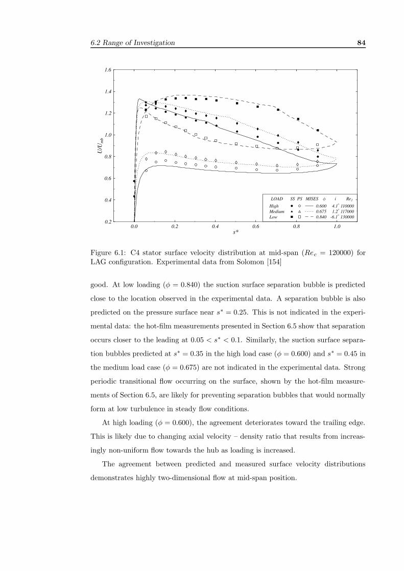
termining velocity from surface pressure are detailed in Section 4.7. Figure 6.2 shows

the influence of turbulence and IGV–stator blade row clocking on the suction surface

velocity distributions at mid-span. The measurements at low turbulence level without

the grid were made by Hughes [83].

0.0 0.2 0.4 0.6 0.8 1.0

s*

0.8

1.0

1.2

1.4

No grid, a/S=0.5No grid, a/S=0.0Grid, a/S=0.5Grid, a/S=0.0

0.8

1.0

1.2

1.4

U/U

mb

0.8

1.0

1.2

1.4

Low Loading ( =0.840)

Medium Loading ( =0.675)

High Loading ( =0.600)

Figure 6.2: C4 stator suction surface velocity distributions at mid-span (Rec =120000). Measurements without grid from Hughes [83].

Time constraints prohibited measuring pressure distributions on the pressure sur-

face since this would have required dismantling the compressor and replacing the

stator blade instrumented with hot-film sensors with the stator blade instrumented

6.5 Hot-Film Surveys 87

with pressure surface tappings. However, this was only a minor inconvenience since

the flow behaviour on the suction surface was of principal interest in this study.

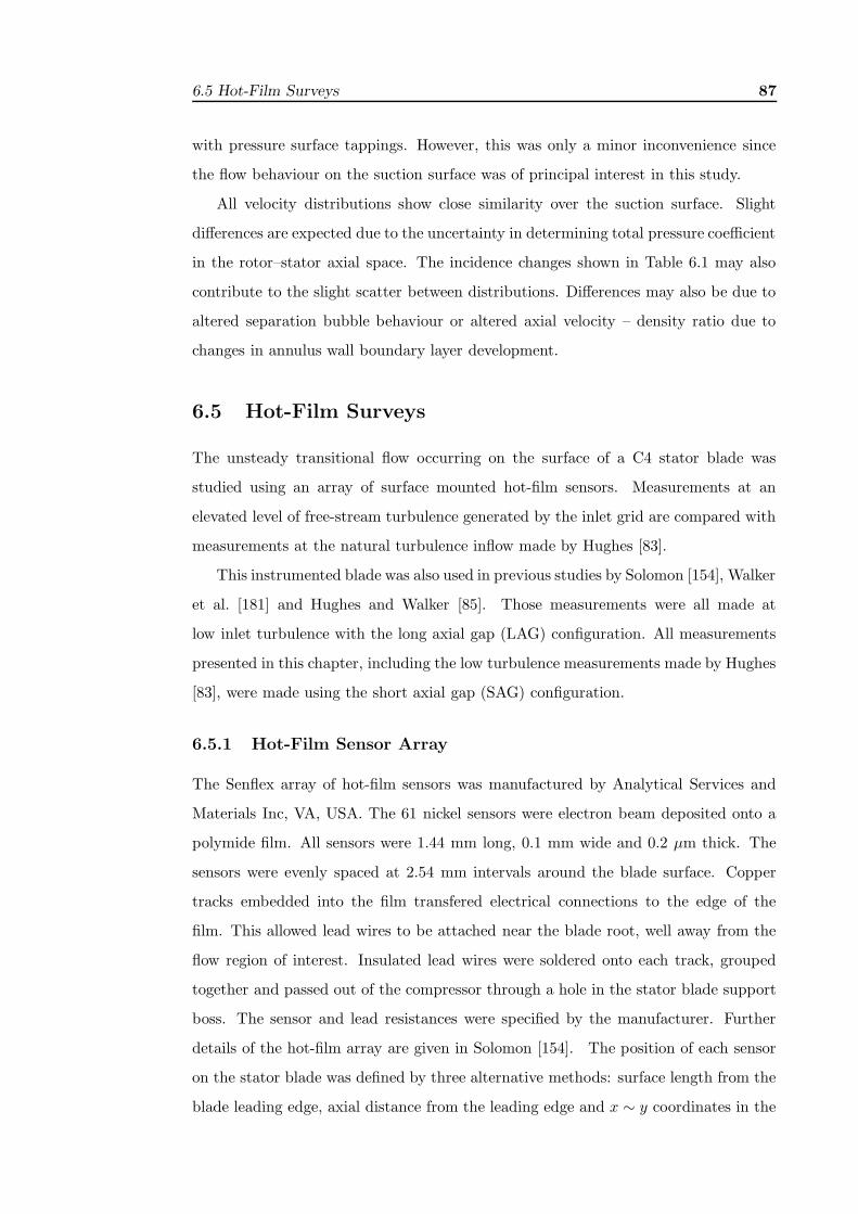
All velocity distributions show close similarity over the suction surface. Slight

differences are expected due to the uncertainty in determining total pressure coefficient

in the rotor–stator axial space. The incidence changes shown in Table 6.1 may also

contribute to the slight scatter between distributions. Differences may also be due to

altered separation bubble behaviour or altered axial velocity – density ratio due to

changes in annulus wall boundary layer development.

6.5 Hot-Film Surveys

The unsteady transitional flow occurring on the surface of a C4 stator blade was

studied using an array of surface mounted hot-film sensors. Measurements at an

elevated level of free-stream turbulence generated by the inlet grid are compared with

measurements at the natural turbulence inflow made by Hughes [83].

This instrumented blade was also used in previous studies by Solomon [154], Walker

et al. [181] and Hughes and Walker [85]. Those measurements were all made at

low inlet turbulence with the long axial gap (LAG) configuration. All measurements

presented in this chapter, including the low turbulence measurements made by Hughes

[83], were made using the short axial gap (SAG) configuration.

6.5.1 Hot-Film Sensor Array

The Senflex array of hot-film sensors was manufactured by Analytical Services and

Materials Inc, VA, USA. The 61 nickel sensors were electron beam deposited onto a

polymide film. All sensors were 1.44 mm long, 0.1 mm wide and 0.2 µm thick. The

sensors were evenly spaced at 2.54 mm intervals around the blade surface. Copper

tracks embedded into the film transfered electrical connections to the edge of the

film. This allowed lead wires to be attached near the blade root, well away from the

flow region of interest. Insulated lead wires were soldered onto each track, grouped

together and passed out of the compressor through a hole in the stator blade support

boss. The sensor and lead resistances were specified by the manufacturer. Further

details of the hot-film array are given in Solomon [154]. The position of each sensor

on the stator blade was defined by three alternative methods: surface length from the

blade leading edge, axial distance from the leading edge and x ∼ y coordinates in the

6.5 Hot-Film Surveys 88

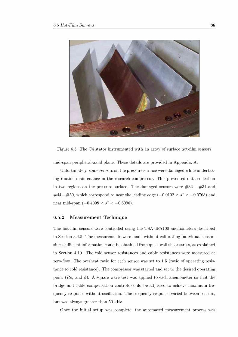
Figure 6.3: The C4 stator instrumented with an array of surface hot-film sensors

mid-span peripheral-axial plane. These details are provided in Appendix A.

Unfortunately, some sensors on the pressure surface were damaged while undertak-

ing routine maintenance in the research compressor. This prevented data collection

in two regions on the pressure surface. The damaged sensors were #32 − #34 and

#44−#50, which correspond to near the leading edge (−0.0102 < s∗ < −0.0768) and

near mid-span (−0.4098 < s∗ < −0.6096).

6.5.2 Measurement Technique

The hot-film sensors were controlled using the TSA–IFA100 anemometers described

in Section 3.4.5. The measurements were made without calibrating individual sensors

since sufficient information could be obtained from quasi wall shear stress, as explained

in Section 4.10. The cold sensor resistances and cable resistances were measured at

zero-flow. The overheat ratio for each sensor was set to 1.5 (ratio of operating resis-

tance to cold resistance). The compressor was started and set to the desired operating

point (Rec and φ). A square wave test was applied to each anemometer so that the

bridge and cable compensation controls could be adjusted to achieve maximum fre-

quency response without oscillation. The frequency response varied between sensors,

but was always greater than 50 kHz.

Once the initial setup was complete, the automated measurement process was

6.5 Hot-Film Surveys 89

started. A short series of readings were taken from each channel to determine the

optimum gain and offset settings for the signal conditioners. Data were acquired using

the Win30DS card detailed in Section 3.4.7. The acquisition process was triggered at

a fixed rotor phase. The anemometer voltages were simultaneously sampled at 50 kHz

and low pass filtered at 20 kHz to prevent aliasing of the signal during the digitisation

process. This procedure was repeated until 512 records were collected, each acquired

on separate revolutions of the rotor. Each record contained 1024 samples. Once data

acquisition was complete, the compressor was brought to rest and the anemometer

voltages were recorded at zero-flow.

Measurements were not made from every hot-film sensor, since sufficient infor-

mation could be provided by measuring every second sensor in regions where flow

behaviour did not change rapidly. This approach was also used by Hughes [83], al-

though different combinations of sensors were used in the present study due to the

damaged sensors reported in Section 6.5.1.

6.5.3 Surface Intermittency Distributions

The hot-film results presented in this Section have been processed using the method

described in Section 4.10. The processed results have been presented in the conven-

tional s∗ ∼ t∗ format where the horizontal axis indicates dimensionless surface length

s∗ and the vertical axis indicates dimensionless time t∗. Particle trajectories at var-

ious fractions of the free-stream velocity have been overlaid to aid with interpreting

the leading and trailing edge celerities of the turbulent strips. The trajectories were

calculated from the surface pressure measurements presented in Section 6.4 using the

method described in Section 4.11.

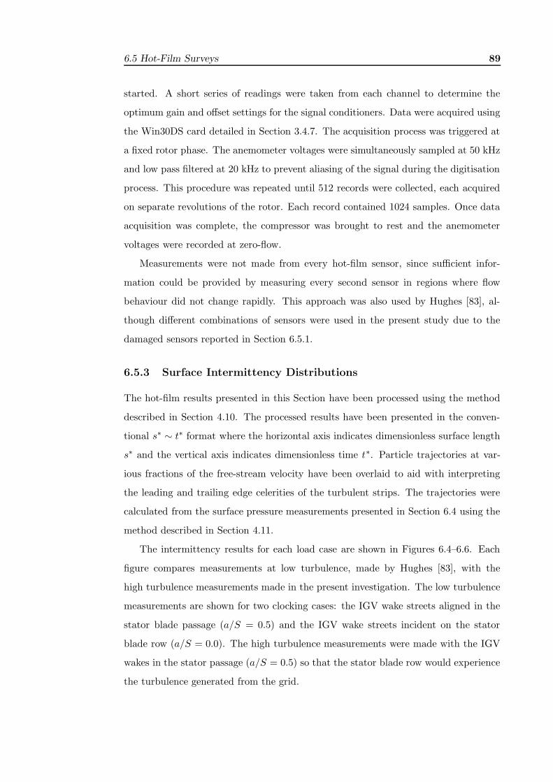
The intermittency results for each load case are shown in Figures 6.4–6.6. Each

figure compares measurements at low turbulence, made by Hughes [83], with the

high turbulence measurements made in the present investigation. The low turbulence

measurements are shown for two clocking cases: the IGV wake streets aligned in the

stator blade passage (a/S = 0.5) and the IGV wake streets incident on the stator

blade row (a/S = 0.0). The high turbulence measurements were made with the IGV

wakes in the stator passage (a/S = 0.5) so that the stator blade row would experience

the turbulence generated from the grid.

6.5 Hot-Film Surveys 90

-0.8 -0.6 -0.4 -0.2 0.0 0.2 0.4 0.6 0.8Pressure Surface ~ s* ~ Suction Surface

0.0

0.5

1.0

1.5

2.0

2.5

3.0

0.0

0.5

1.0

1.5

2.0

2.5

3.0

t*

0.0

0.5

1.0

1.5

2.0

2.5

3.0

0.0

1.0

<>

High Tu (IGV wakes in stator passage g/S=0.5, a/S=0.5)

Low Tu (IGV wakes on stator row a/S=0.0)

Low Tu (IGV wakes in stator passage a/S=0.5)

Figure 6.4: C4 stator surface intermittency distribution at high loading (φ = 0.600,Rec = 120000). Colour filled contours show ensemble average intermittency (〈γ〉), linecontours show probability of relaxing flow in 1% intervals, and particle trajectories at1.0U, 0.88U, 0.7U and 0.5U

6.5 Hot-Film Surveys 91

-0.8 -0.6 -0.4 -0.2 0.0 0.2 0.4 0.6 0.8Pressure Surface ~ s* ~ Suction Surface

0.0

0.5

1.0

1.5

2.0

2.5

3.0

0.0

0.5

1.0

1.5

2.0

2.5

3.0

t*

0.0

0.5

1.0

1.5

2.0

2.5

3.0

0.0

1.0

<>

High Tu (IGV wakes in stator passage g/S=0.5, a/S=0.5)

Low Tu (IGV wakes on stator row a/S=0.0)

Low Tu (IGV wakes in stator passage a/S=0.5)

Figure 6.5: C4 stator surface intermittency distribution at medium loading (φ = 0.675,Rec = 120000). Colour filled contours show ensemble average intermittency (〈γ〉), linecontours show probability of relaxing flow in 1% intervals, and particle trajectories at1.0U, 0.88U, 0.7U and 0.5U

6.5 Hot-Film Surveys 92

-0.8 -0.6 -0.4 -0.2 0.0 0.2 0.4 0.6 0.8Pressure Surface ~ s* ~ Suction Surface

0.0

0.5

1.0

1.5

2.0

2.5

3.0

0.0

0.5

1.0

1.5

2.0

2.5

3.0

t*

0.0

0.5

1.0

1.5

2.0

2.5

3.0

0.0

1.0

<>

High Tu (IGV wakes in stator passage g/S=0.5, a/S=0.5)

Low Tu (IGV wakes on stator row a/S=0.0)

Low Tu (IGV wakes in stator passage a/S=0.5)

Figure 6.6: C4 stator surface intermittency distribution at low loading (φ = 0.840,Rec = 120000). Colour filled contours show ensemble average intermittency (〈γ〉), linecontours show probability of relaxing flow in 1% intervals, and particle trajectories at1.0U, 0.88U, 0.7U and 0.5U

6.5 Hot-Film Surveys 93

The grid wakes were aligned in the centre of the IGV blade row passage (g/S = 0.5)

which results in the most uniform turbulence condition. The effect of clocking the

IGV blade row relative to the turbulence grid on stator intermittency distribution is

discussed in Part (c) of this Section

(a) Observations at Low Turbulence

The intermittency distributions for the high and medium loading cases are shown in

Figs 6.4 and 6.5. The two clocking cases at low turbulence are shown in the centre

and top sections. With the IGV wakes in the stator passage (a/S = 0.5), well-

defined wake-induced transitional strips are present on both the suction and pressure

surfaces. These strips are immediately followed by relaxing flow as indicated by the

line contours. The strength of relaxing flow is significantly greater on the suction

surface. This is likely a reflection of the stronger development of the transitional

strips occurring on the suction surface. In this case, the suction surface transition

between wake-induced strips occurs at s∗ = 0.7. This is consistent with the stator

blade row experiencing pockets of very low turbulence between rotor wakes (typically

0.5%) as shown in Chapter 5. Immersing the stator blade row in the IGV wake street

(a/S = 0.0) causes the stator to experience higher turbulence between rotor wakes

(typically 2−3%). Correspondingly, the transition between wakes moves upstream to

s∗ = 0.3. The calming effect is observed to more weakly inhibit transition. This effect

wears off before the arrival of the next wake-induced strip and the transition onset

moves upstream to s∗ = 0.3.

Clocking is observed to have little influence on the pressure surface intermittency

distributions at these loading cases. It may be that the apparent transitional strip

could be rather a laminar layer buffeted by the rotor wake jet turbulence impinging

on the blade surface. The limit for pressure surface transition onset may be set by

Reθminfor sustained turbulent flow.

The blade surface intermittency distribution for low loading is shown in Fig. 6.6.

The flow over the suction surface experiences a favourable pressure gradient from the

leading edge to approximately s∗ = 0.3, as shown in Fig. 6.1. This has a stabilising

effect on the boundary layer that delays transition further along the surface than in the

other loading cases. The discontinuity in surface velocity shown in Fig. 6.1 indicates

the presence of a large separation bubble at s∗ = 0.7. This was confirmed by hot-film

measurements made by Solomon [154]. These measurements, expressed in terms of

6.5 Hot-Film Surveys 94

log ensemble quasi wall shear stress, showed a sudden drop between s∗ = 0.5 and

s∗ = 0.8, which is consistent with a region of separated flow. The separation point

occurs upstream from the detected onset of wake-induced transition. This suggests

that wake-induced transition occurs in the separated shear layer rather than in the

attached boundary layer. The suction surface intermittency distribution showed little

variation with clocking position for this compressor loading.

High levels of intermittency are observed on the pressure surface in the low loading

case. Here, an interesting clocking effect is observed with the IGV wakes in the

stator passage (a/S = 0.5). Wake-induced transitional strips occur very close to the

leading edge produce an associated region of calmed flow that extends to s∗ = −0.7

before being overtaken by turbulent flow. The wake-induced transition temporarily

suppresses formation of a leading edge separation bubble extending to s∗ = −0.3.

Immersing the stator blade row in the IGV wake street reduces the extend of separation

and causes transition between strips to move closer to the leading edge (s∗ = −0.03),

thus resulting in almost continuous turbulent flow over the pressure surface.

(b) Observations at high turbulence

The lower part of Figs 6.4–6.6 shows the intermittency distribution at high turbulence

level with the turbulence grid. Although the turbulence profile at inlet was quite

uniform, as shown in Section 5.3, the IGV wake street was deliberately aligned in the

stator passage (a/S = 0.5). This ensured that the stator blade row was exposed to

turbulence generated from the grid, rather than from IGV wake street.

The general features of the intermittency distributions for each load case closely

resemble the low turbulence case with the mid-span stator blade row element immersed

in the IGV wake street (a/S = 0.0). At medium and high loading, the suction surface

transition between the rotor wake-induced transitional strips moves closer toward the

leading edge. The regions of calmed flow following the strip are also more sharply

defined.

The small incidence increases noted in Section 6.3 have the effect of moving tran-

sition upstream on the suction surface, particularly in the high and medium load

cases. However, such changes would be relatively minor and the observed differences

in intermittency distribution are considered to be primarily due to altered turbulence

properties. Other minor differences, particularly on the pressure surface close to the

leading edge are attributed to the use of different hot-film sensors (See Section 6.5.2).

6.5 Hot-Film Surveys 95

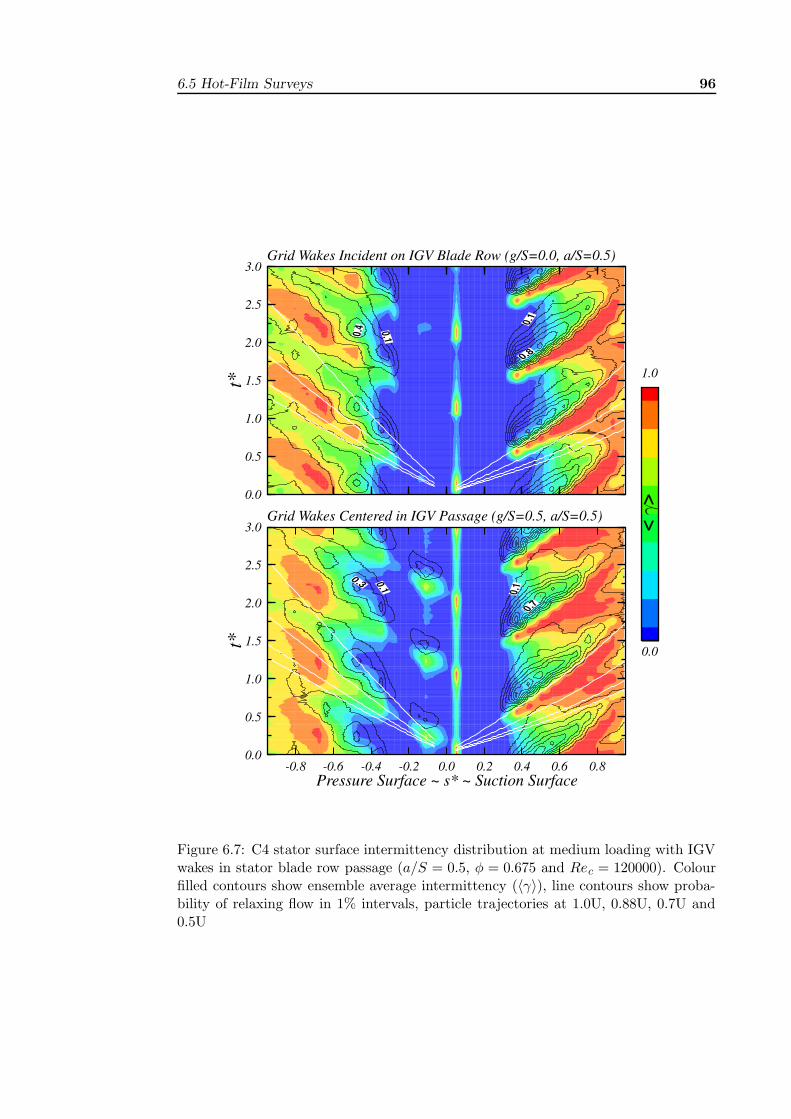
(c) Grid–IGV Clocking Effect

Figure 6.7 shows the effect of clocking the IGV blade row relative to the turbulence

grid on the stator surface intermittency distribution. In these measurements, a relative

alignment was maintained between the IGV and stator blade rows. Both the IGV and

stator blade rows were moved together to change the alignment between the IGV and

turbulence grid (g/S). For consistency with results presented in the previous Part (b)

of this Section, the IGV wakes were centred in the stator blade row passage so that

the stator blade row experienced turbulence generated from the grid rather than the

IGV blade row (a/S = 0.5).

The results show a slightly greater extent of turbulent flow on both surfaces in the

case where the grid wakes were centred in the IGV blade row passage (g/S = 0.5).

This is consistent with the inlet turbulence measurements presented in Section 5.3.1

which show this configuration results in a greater turbulence level between IGV wake

streets.

(d) Time-Averaged Intermittency Distributions

Useful information is also provided by comparing long term averaged intermittency

distributions as shown in Fig. 6.8. These were obtained by averaging ensemble aver-

aged intermittency (γ) over an integral number of rotor passing periods. The uneven

spacing between data points reflects the fact that not every hot-film sensor was mea-

sured.

The highest average intermittency occurs in the high turbulence case using the

turbulence grid. The distribution closely resembles the low turbulence case with the

stator blade row immersed in the IGV wake street. This is consistent with the trend

shown by the ensemble average s∗ ∼ t∗ contour plots in Figs 6.4–6.6.

The local intermittency peak near the leading edge may be genuine turbulent flow

which rapidly decays, spurious detections caused by external turbulence buffeting the

thin boundary layer, or incidence fluctuations associated with the rotor wake passage.

6.5 Hot-Film Surveys 96

-0.8 -0.6 -0.4 -0.2 0.0 0.2 0.4 0.6 0.8Pressure Surface ~ s* ~ Suction Surface

0.0

0.5

1.0

1.5

2.0

2.5

3.0

t*

0.0

0.5

1.0

1.5

2.0

2.5

3.0

t*

0.0

1.0

<>

Grid Wakes Centered in IGV Passage (g/S=0.5, a/S=0.5)

Grid Wakes Incident on IGV Blade Row (g/S=0.0, a/S=0.5)

Figure 6.7: C4 stator surface intermittency distribution at medium loading with IGVwakes in stator blade row passage (a/S = 0.5, φ = 0.675 and Rec = 120000). Colourfilled contours show ensemble average intermittency (〈γ〉), line contours show proba-bility of relaxing flow in 1% intervals, particle trajectories at 1.0U, 0.88U, 0.7U and0.5U

6.5 Hot-Film Surveys 97

-0.8 -0.6 -0.4 -0.2 0.0 0.2 0.4 0.6 0.8Pressure Surface ~ s* ~ Suction Surface

0.0

0.2

0.4

0.6

0.8

1.0

grid, a/S=0.0no grid, a/S=0.5no grid, a/S=0.0

0.0

0.2

0.4

0.6

0.8

1.0

0.0

0.2

0.4

0.6

0.8

1.0

Low Loading ( =0.840)

Medium Loading ( =0.675)

High Loading ( =0.600)

Figure 6.8: Time-mean ensemble averaged intermittency distribution for the C4 stator(γ)

6.6 Conclusions 98

6.6 Conclusions

This chapter has compared the transitional behaviour on a C4 stator blade under the

natural low turbulence inflow conditions with that under artificially generated high

turbulence conditions characteristic of an embedded stage in a multi-stage machine.

The intermittency distributions at the natural low turbulence inflow were strongly

influenced by blade row clocking. Aligning the IGV wakes in the stator passage

exposed the stator to pockets of low turbulence. The corresponding intermittency

distribution showed a very high levels of periodicity. Immersing the stator blade row

in the IGV wake street resulted in the suction surface transition between wake-induced

strips moving upstream. The intermittency distribution resulting from use of the

turbulence grid closely resembled the test case without the grid where the IGV wake

street was incident on the stator blade row. This suggests that a 1.5-stage machine can

simulate the transitional flow behaviour on an embedded blade row element without

artificially increasing the inlet turbulence.