1

C. LAB 3. MINEQL LABORATORY  

This lab introduces you to the use of the computer program MINEQL for solving chemical equilibrium problems.  The program can handle numerous components, temperature corrections, and corrections for ionic strength; it is quite useful in solving complex chemical equilibrium problems.  The program also can be used to simulate experiments (e.g., titrations) and to predict adsorption.  It is limited by its thermodynamic database (the solutions to problems are only as accurate as the thermodynamic database in the program) and by the fact that it lacks the capability of solving chemical kinetics problems.  You may use this program for any remaining problem sets and labs throughout the term; a number of you are likely to use a program similar to this in a future job setting. 

We will use the program to examine aspects of equilibrium that are tedious to calculate by hand.  This first introduction is intended to acquaint you with the structure of the program, and the details of how to begin to use it.  Remember that computer programs are no substitute for your head.  The computer cannot tell you whether the answer it spits out is correct.  You have to develop the ability to estimate approximate answers, and then to refine those estimates with the computer.  To make such estimates, you need a conceptual understanding of the problem.  In all problems for this program that you will be given in problem sets, you will be asked for an approximate answer determined without the computer program.   

How does such a program work?  It follows an iterative procedure similar to what you would use in solving the problem by hand, except that it uses a numerical, matrix method (Newton‐Raphson) for solving the multiple simultaneous equations.  Specifically, the program sets up the matrix with the equations for the equilibrium constants.  It then uses your input values for total ion concentrations as its guess of the free concentrations and solves the matrix.  Next the program compares its results with the mass balance equations (including the proton condition) and, if the mass balance is not satisfied, it adjusts the starting concentrations and resolves the matrix. 

To learn how to use the program you will walk through the steps in the attached Tutorial.  Do not proceed unless you get the results given in the manual.  The program is user‐friendly, and the on‐line help mode will answer most of your questions regarding the use of the program.    Introduction to MINEQL 

As you will learn later in the course, solving equilibrium chemistry problems involves relatively simple but tedious algebra.  Most problems involve numerous unknowns (generally, the concentrations of chemical species; e.g., [Ca2+] or [CO3

2‐]) and, therefore, they require solving numerous, simultaneous equations.  For simple problems, the equations are linear, but frequently they are quadratic or cubic.  The computer program merely provides an easy method for solving this algebra using a numerical method.  To use the program, you still have to know how to set up the problem and how to estimate an approximate answer.  Components and Species Used in Solving Chemical Equilibrium Problems 

The first step in setting up a problem is identifying the unknowns.  In the vast majority of cases in this course, the unknowns are the concentrations of chemical species.  This first step 

2

involves identifying the chemical species that are present in the system and then determining which of these are involved in equilibrium reactions.  That may sound intimidating now, but soon this step will be quite easy.  In MINEQL, the simplest dissolved chemical species are called components or Type I species.  The components in a system are a set of chemical entities that are used to create every species by chemical reactions involving the components.  No other components can be used to represent a particular component other than itself.  The first step in running the program is to enter (from a table) the components.  For example, rather than defining bicarbonate (HCO3

‐) as a component, this complex is broken into its two constituent components H+ and CO3

2‐.  Similarly, if the problem involves addition of a solid to water (e.g., cement, CaCO3•H2O), the components would be the dissolved species that may be formed from this solid (in this case, Ca2+, CO3

2‐, and H2O are selected as components).  The components H2O and H

+ are automatically selected in all problems. Components may undergo several types of reactions to form other "classes" of 

compounds.  The formation of complexes or Type II species was mentioned above.  Complexes are dissolved species that consist of two or more components.  Examples include acids (e.g., HCl, HNO3, and H2SO4 ), bases (e.g., NaOH, NH4OH), and other soluble charged or uncharged groupings of components (e.g., HCO3

‐, HSO4‐, CuCO3

o).  A rather strange complex is OH‐; in the terminology of MINEQL, OH‐ is a complex of water and a negative proton.   

Another class of compounds are the dissolved solids or Type V species.  A dissolved solid is a salt that is present at a concentration below its solubility limit, but has the potential to precipitate if the concentrations reach the solubility limit.  If it were allowed to precipitate in the program, it would then become a Type IV or precipitated solid.  Precipitated solids may redissolve if concentrations in solution are low enough.  (This will be explained in detail later in the course.) 

Often, we know that a chemical species does not form in the environment even though it is thermodynamically possible for it to form.  There also are cases where we know that a solid phase is present, but it reacts so slowly that it need not be considered in the estimation of equilibrium conditions.  Because MINEQL predicts what is thermodynamically favorable, the program would erroneously predict that such species would form or react unless we were to prevent it from doing so.  It is for these cases that MINEQL has Type VI species or species not considered.  The program ignores these species when carrying out mass balances, but it nevertheless calculates the concentration of each of these species. So the final concentrations of these species are not relevant to the calculation of the equilibrium composition in the current problem. Sometimes these concentrations are of interest to us, even though they are not often the concentrations of real species in the equilibrium solution.  

The final category of chemical species are those that are present at a known concentration; these are termed fixed or Type III species.  Often we know that the pH is buffered at a constant value; it would be erroneous to allow the program to calculate the H+ concentration as if it were a free variable.  Instead, we tell the program that the concentration is fixed.  Similarly, if a large quantity of a solid phase is present such that it cannot possibly all dissolve, then the concentrations of the component ions will be held at the solubility limit of this solid.  Another common example involves open systems; the supply of gases from the atmosphere is unlimited and hence the concentration of the dissolved gas in an open system is 

3

considered to be in equilibrium (fixed at a give value) with the concentration of the gas present in the atmosphere.  Tableau 

Tableaux (plural – French meaning “Table”) are useful in solving chemical equilibrium problems, and they are used in MINEQL.  A tableau (singular) is a matrix of stoichiometric coefficients. The columns of the table represent chemical components, while the rows of the table represent chemical species. In addition to stoichiometry, a tableau also includes thermodynamic data that is associated with each reaction plus the total concentrations associated with each chemical component. 

The best way to understand the tableau is with an example. Let’s assume we have a solution comprised of 1.0 × 10‐3 M Na2CO3, 5.0 × 10‐4 M NaAc, and 7.0 × 10‐4 M HCl. The components in the system are H2O, H

+, Na+, Ac‐, Cl‐, and CO32‐. In the following expressions, 

TOTA is the total molar concentrations of species A if A has been chosen as a component. [ ]T is the molar concentration of the chemical compound used in the system.  

[ ]2 2 TH O H O 55.56TOT M= =  

[ ] 4T

H HCl 7.0 10TOT M−= = ×  

[ ] [ ] 32 3 T T

Na 2 Na CO NaAc 2.5 10TOT M−= + = ×  

[ ] 4T

Ac NaAc 5.0 10TOT M−= = ×  

[ ] 4T

Cl HCl 7.0 10TOT M−= = ×  

[ ]2- 33 2 3 T

CO Na CO 1.0 10TOT M−= = ×  

 The following reactions take place in the system:  

+ -2H O H OH+     Log K = ‐14.00 + 2- -

3 3H CO HCO+     Log K = 10.33 + 2-

3 2 32H CO H CO+   Log K = 16.68 + -H Ac HAc+     Log K = 4.76 

 The species expected to be present at equilibrium include chemicals that are identical to all six components plus OH‐, HCO3

‐, H2CO3, and HAc. The tableau for the system is written as:  

Species  H2O  H+  Na+  Ac‐  Cl‐  CO32‐  LogK 

H2O  1  0  0  0  0  0  0.00 H+  0  1  0  0  0  0  0.00 Na+  0  0  1  0  0  0  0.00 Ac‐  0  0  0  1  0  0  0.00 Cl‐  0  0  0  0  1  0  0.00 

CO32‐  0  0  0  0  0  1  0.00 

4

OH‐  1  ‐1  0  0  0  0  ‐14.00 HCO3

‐  0  1  0  0  0  1  10.33 H2CO3  0  2  0  0  0  1  16.68 

HAc  0  1  0  1  0  0  4.76 Total Conc. (M)  55.56  7.0×10‐3  2.5×10‐3  5.0 × 10‐4  7.0×10‐3  1.0 × 10‐3    

This tableau contains all the necessary information for the equilibrium problem. A complete set of equations can be readily written. Mole balances (from each column) can be written as:  

[ ] -2 2H O H O OH 55.56TOT ⎡ ⎤= + =⎣ ⎦  

[ ] [ ]+ - - 33 2 3H H OH HCO 2 H CO HAc 7.0 10TOT −⎡ ⎤ ⎡ ⎤ ⎡ ⎤= − + + + = ×⎣ ⎦ ⎣ ⎦ ⎣ ⎦  

+ 3Na Na 2.5 10TOT −⎡ ⎤= = ×⎣ ⎦  

[ ]- 4Ac Ac HAc 5.0 10TOT −⎡ ⎤= + = ×⎣ ⎦  - 3Cl Cl 7.0 10TOT −⎡ ⎤= = ×⎣ ⎦  

[ ]2- 2- - 33 3 3 2 3CO CO HCO H CO 1.0 10TOT −⎡ ⎤ ⎡ ⎤= + + = ×⎣ ⎦ ⎣ ⎦  

 The mass action equations that form the species are:  

{ } { }{ } 114210OH H O H

−− − +=  

{ } { }{ }- 10.33 + 2-3 3HCO 10 H CO=  

{ } { } { }216.68 + 2-2 3 3H CO 10 H CO=  

{ } { }{ }4.76 +HAc 10 H Ac=  

 There are 10 unknowns in this equilibrium problem (i.e., the concentrations of each of the 10 species) and 10 equations (6 mole balances and 4 mass laws). The equations can be solved by applying an appropriate numerical method. Fortunately, we do not need to do this. The MINEQL software does this for us. 

5

 MINEQL Tutorial   Starting MINEQL 

The  computer  program MINEQL+  is  installed  on  all  departmental  PCs.  To  start  the program,  click Start   programs   classes   environmental classes   MINEQL+.   Choosing Components 

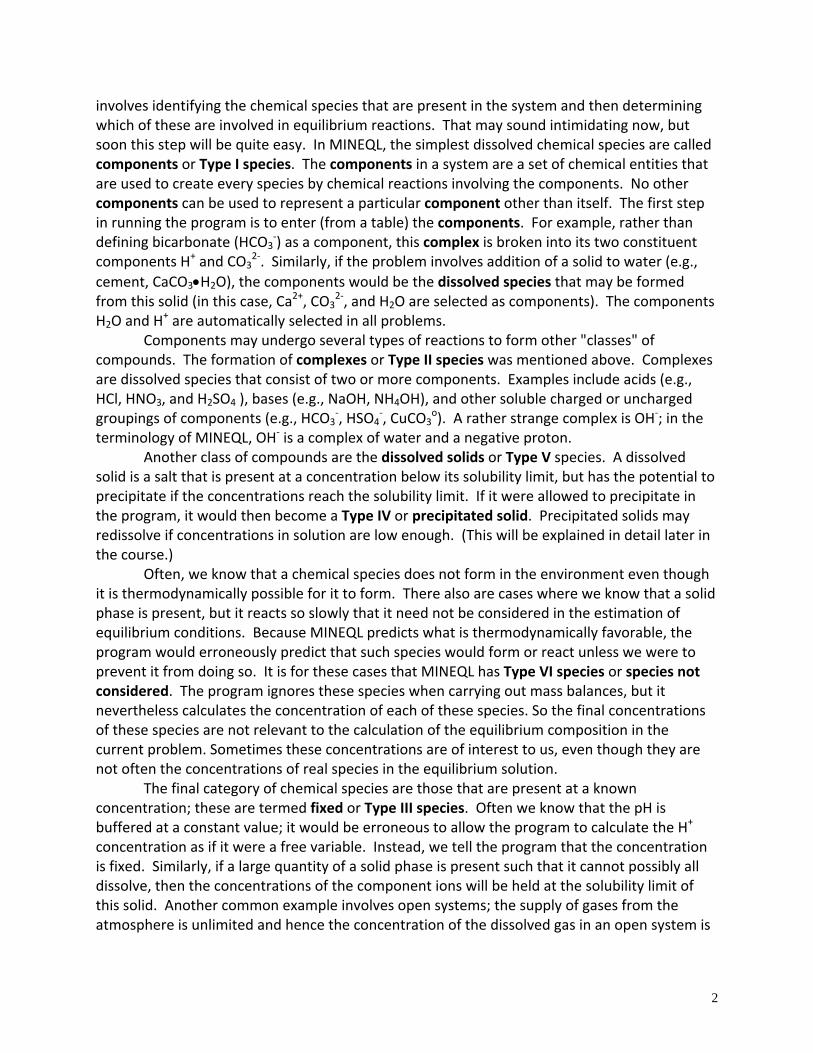
The Autopilot should initialize when the program starts up. This in turn should open the Select Components  tool. This  is a window entitled  “Chemical Components Selection Module” that contains various anions, cations and neutral molecules (Figure 1). In this module, one can choose the various basic components that make up a system by simply clicking on the boxes to the left of the desired component. The ions are arranged row‐wise in an alphabetical order.  

By default, both H2O and H+ are always selected. This is because there are many ways to write down a particular reaction. For example, consider the following reaction:  HCO3

‐       H+  +  CO32‐                    log K1 

 A second way to write the above reaction would be:  HCO3

‐  +  OH‐      H2O  +  CO32‐      log K2 

 MINEQL+ always writes this original reaction as if the species of interest is being formed:   H+   +   CO3

2‐          HCO3‐                 log K3 (=  ‐ log K1) 

 and has the value log K3 stored in its database for that reaction.   

6

 Figure 1. Chemical Components Selection Module Window  More about the chemical component selection module: 

In addition to the various anions and cations, the component selection module contains the following 5 buttons right below the title bar:  

1. Scan THERMO: Press this button once you are done selecting the components. The computer will automatically search the default thermodynamic database and come up  with  a  list  of  thermodynamically  feasible  reactions  and  the  appropriate equilibrium constants. 

2. New:  Press  this  button  if  you  want  to  deselect  all  selected  components.  This obviates the necessity to de‐click all the components for the next calculation. 

3. Return:  Press  this  button  if  you  want  to  directly  go  into  the  next  menu.  The computer then uses the components selected. This button is mainly used if you want to perform further calculations on a previously defined system. 

4. Edit Menu: Use this button to define new components. All components that you’ll be working with in this course are already in the components menu.  

5. Help: Press this button  if you need some help anytime during the course of a run. The menu is fairly extensive and should help you solve most of your problems. 

 The  four  examples  provided  below  illustrate  how  to  use  MINEQL  to  determine 

equilibrium activities.   Example 1: Equilibrium speciation in water

Exercise: Suppose a container of water has some calcium phosphate in it. Suppose it is known that the total [Ca2+] equals 10-4 M, total [PO4

3-] equals 5 × 10-5 M and the pH of the solution is 5.20. What is the speciation of phosphate in this water sample under equilibrium conditions?

Answer: The basic components that make up this solution are H+, OH-, Ca2+ and PO43-.

Since it is possible to calculate the OH- activity from H+ activity, you need not specify both H+ and OH-. Since this is a Ca-PO4 system, we will need to include these components in the Select Components tool in addition to H2O and H(+). Use the mouse to click on Ca(2+) and then PO4(3-) from the list of components shown on the screen. Again, using your mouse, press the Scan thermo button in order to extract the reaction data you’ll need to run this problem.

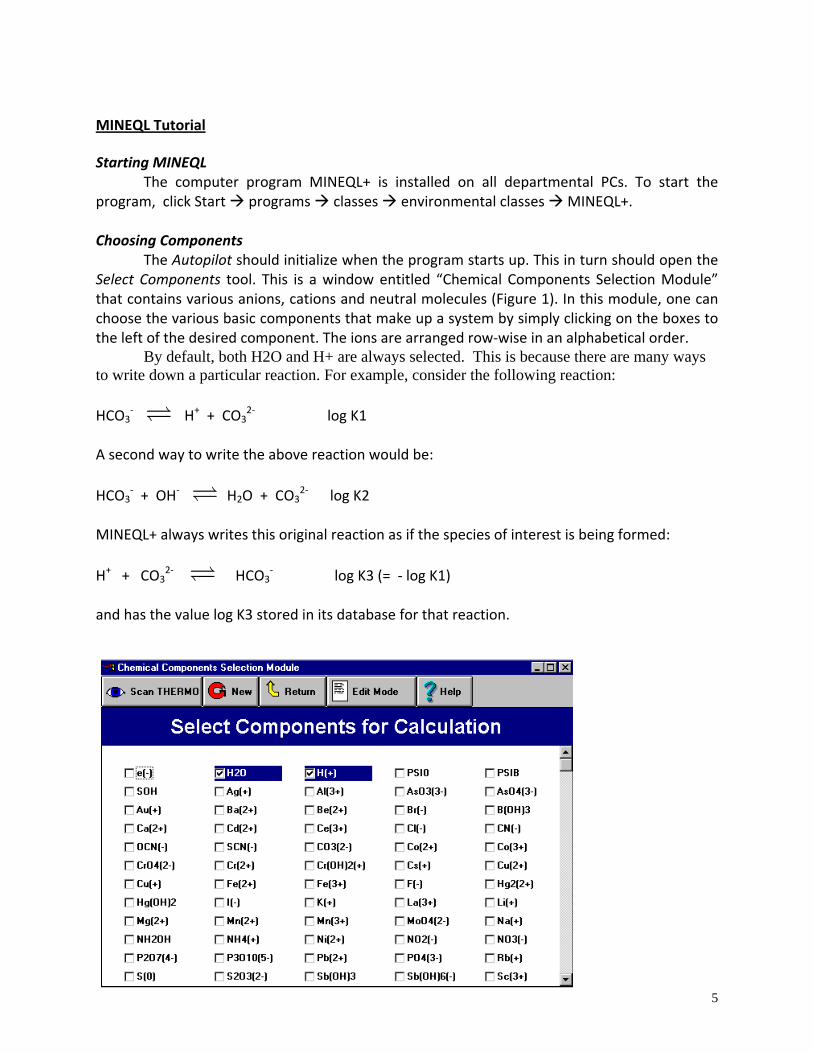
Pressing the “Scan Thermo” or “Return” buttons will take you to a Tableau tool titled Type II – Aqueous Species (see Figure 2). In this and the next few windows, you can examine the species that make up your system, and enter the total component concentrations that will be used to solve the problem.

7

Figure 2. Aqueous Species Window

Types II through VI tableaux contain three main columns: (i) Left column: name and charge of the species that can be formed from the components that you specified in the previous menu; (ii) middle panel: stoichiometry of species in left panel formed from the various species you selected in the previous menu; and (iii) right two columns: Log K and ΔHi° values for the formation of the species in the left column. For the above mentioned example, you should see the window shown in Figure 2 for Type II – Aqueous Species.

There are 8 aqueous species listed in the left column that can be formed from H2O, H(+), Ca(2+) and PO4(3-). The next main column lists the stoichiometric coefficients of the reactants (components) required to form the species listed under the “name” column. For example: 0 H2O + 1 H(+) + 1 Ca(2+) + 1 PO4(3-) CaHPO4 (aq) specifies the number of H2O, H(+), Ca(2+) and PO4(3-) molecules necessary to form one CaHPO4 molecule. The equilibrium constant for this reaction is 1015.035. One can enter the total concentrations of the species present in one’s system in the last row under “Total Conc. (M) ”. The value can be entered simply by highlighting the displayed value and typing in the new value, and pressing Return. For the above example, in order to enter the total calcium ion concentration, simply highlight the value under the Ca(2+) column and type in 1E-4 (10-4 M concentration). One can do the same thing for PO4(3-) and H(+)(from [H+] = 10-pH). Other ways for entering the concentrations of species are possible using the Wizard Tool, which will be discussed later on.

Once you are done entering all the values, press the Close button located below the title bar. The Tableau tool will disappear and a software tool will appear that will allow you to examine other types of reaction data in your system. Select the type of species you wish to examine and press the Yes button to open the appropriate tableau. For example, to look at the dissolved solids present in the system, make sure that the Dissolved Solids button is selected and press the Yes button to examine the tableau for dissolved solids. This tableau contains a list of solids that have the potential to precipitate if their solubility product is exceeded. For the above mentioned example, the window shown in Figure 3 appears.

8

Figure 3. Dissolved Solids Window

Similar to Type II menu, each row gives all the necessary information for a given

reaction. For example, the top line contains all the information necessary to describe the formation of lime (CaO (S)). Ca2+ + H2O CaO (S) + 2 H+ Click on the Close button and this time press the No button to stop opening the Tableau Tool. The RunTime manager will open at this point. More about the Tableau Tool for Type II - VI Species: In addition to the names of species, all the tableau tool windows contain the following buttons:

1. Insert: Use this button to insert any compounds that were either not considered under any

of the species (Type II, III, etc.) or to move a compound FROM a species of another type to the present tableau.

2. Delete: Use this button to delete compounds that you do not want to consider in your system. To delete a compound, use the scroll button on the right side to highlight the compound of choice and press delete. Pressing delete will remove the compound from the potential list of compounds that are formed. These species will not be available for future calculations. Another option to accomplish the same objective would be to move that

9

compound to “Species Not Considered”(discussed next). In this case, it is always possible to move the compound back in case you want to perform calculations involving this compound.

3. Move: Use this button to move a compound from a particular Species type to another. For example, the concentration of H3PO4 in this example is pretty small. You could remove the species from the system without causing any apparent change in the concentrations of the other species. To accomplish this, move this compound to Type VI species (Species Not Considered), highlight the compound by scrolling down and press “move”. The Tableau Switch Tool should appear with the following four species types listed: Aqueous complexes, Fixed Entities, Dissolved Solids and Species Not Considered. Some of the fields might not be highlighted, implying that the species cannot be moved to these fields. Click on the radio button to the left of Species Not Considered to move the compound to this field.

4. Close: Use this button to close the displayed window and move to the next one. For example, pressing the Close button while in the Type II – Aqueous Species window will take you to the Tableau Switch Tool window.

5. Wizard: The wizard is a tool for entering the concentrations of species, specifying/calculating the pH of the solution, specifying/calculating the total carbonate/alkalinity of the system, etc. among other things. Pressing the Wizard button opens a window entitled Calculation Wizard. This wizard consists of 5 subsections consisting of the following: (a) Totals listing the components you selected in the Component Selection Tool (minus H2O, H+ and CO3(2-)) and a box to the right of each component into which you can enter the total concentration of that particular component. (b) pH showing two possible calculation types viz. pH is supplied by user or pH is calculated by MINEQL+. One can enter the pH in terms of molar units or as pH. If pH is to be calculated by MINEQL+, the box next to “Base pH calculation on Electroneutrality” should be checked. In this case, fix pH at a value of 5.20. (c) CO2 showing two possible calculation types viz. open to the atmosphere and closed to the atmosphere. When the system is open to the atmosphere, you can specify the partial pressure of CO2 in the atmosphere in log units. On the other hand, when the system is closed to the atmosphere, the carbonate in the system can be entered either as total carbonate in the system (sum of [H2CO3

*], [HCO3-] and [CO3

2-]) or you can estimate the total alkalinity of the system by specifying the pH and alkalinity of the initial system. The computer then will automatically calculate the concentrations of [H2CO3

*], [HCO3-] and [CO3

2-] for your system. (d) Solids Mover showing a list of possible solids that are in your system. This option is used to specify solids that are present in the system at all times and which control the concentrations of other species in the system. (e) Redox showing a list of possible reactions that involve electron transfer.

6. Help: On-line help.

Runtime Manager The RunTime Manager window is shown in Figure 4. Every calculation requires a

unique output file name. Specify a name in the Output Data Name box below the title bar. The program will automatically append .MDO (MINEQL Data Output) to the file name once it starts the run. You’ll need the name of this file to view the results of your calculation.

10

Figure 4. RunTime Manager Window

In the Runtime Manager, specify ionic strength corrections, temperature corrections, take adsorption effects into account, and set the convergence criteria for the calculations. There are three options listed under ionic strength corrections. Setting the ionic strength corrections to Off assumes ideal behavior, i.e., the activity of a compound is equal to its concentration. Clicking the Calculated button tells the program to compute ionic strength of the solution and consider non-ideal behavior of species in the calculations. You can also set the ionic strength of a solution to a certain value. In this case, the ionic strength should be entered in Molar units.

Temperature has an effect on the activities of species as well as the equilibrium constants. As before, you can either turn off this feature or enter a measured value in units of degrees Centigrade. The adsorption model box is used to specify the type of adsorption isotherm while the criteria button is used to specify the default convergence limits for the various calculations. Also, it is alright to perform the calculations using the default convergence criteria. Setting stricter convergence limits tends to increase the time required for completing the calculations. In this example, set ionic strength and temperature corrections Off, and adsorption model None. The Runtime Manager also contains the following 5 buttons:

1. Run: Press this button to start the calculation. After a few seconds, the calculation will be completed and the Output Manager will appear.

2. Cancel: Press this button to start all over again. 3. Wizard: Same as explained above. You can enter the concentrations of the different

components from the Runtime Manager. 4. Multirun: Press this button to do a series of calculations on one or more variables. This

is the ideal tool to study the effects of a titration, as titrations usually involve changing the pH of a solution by adding an acid or a base. The Multirun Manager should appear on

11

clicking the Multirun button. By default, the Type of Calculation is set to Single Run. If you perform a multirun, you’ll have to use the combo box to select the type of the multirun (example: titration). We’ll discuss an example later on.

5. Help: Online help. Output Manager

The Output Manager window is shown in Figure 5. It allows you to: (i) extract speciation output from any perspective and display it in a tabular format; (ii) display the header, log, and the multirun files; (iii) generate graphical output of speciation data (via the Graphic Manager); (iv) generate special reports (e.g., calculate alkalinity, or extract special types of data like ionic strength or saturation index).

Figure 5. Output Manager Window

In the upper-left-hand corner of the screen there is a group of selection buttons, called the

Output Type group, which allow you to choose what type of output you want to display. This group of selection is connected with the View button located at the lower left of the screen. When you use the View button you can display the type of output that you have selected. There are five selection buttons in the Output Type group:

The Header is a concise representation of the input problem, including the date and time of the calculation, a listing of the calculation’s overall assumptions (i.e., the use of electroneutrality assumptions, temperature and ionic strength corrections, or the use of a surface model), the convergence criteria, and the total concentration that was input for each chemical component.

The Log contains a running output of miscellaneous data and error messages that may occur while processing the data. For a normal run, without error message, it is not important to refer to the log file.

The Multirun Variables store the variables in a multirun calculation (i.e., titration). For a titration calculation, the numbers displayed in this table will reflect the range of values that

12

were set using the MultiRun Magnager. As a result, MDO’s for single calculations will not have a multirun member.

The Component Groups selection is associated with two different areas in the Output Manager. First, you must select which component you want to view. This selection is accomplished by clicking off the component from the list located in the middle of the screen, right below the Data Object. Next, you must select the perspective from which you wish to view the data. In the low middle portion of the screen is a group box that contains three options for viewing the data. This box will only become active when the component groups option has been selected. Each option has a combo box button (accessed with the down arrow) for more options. The three options are: (i) Obs. × Variables: gives the concentration, LogC, LogK, % total and stoichiometry for any one species. For instance, if you select Ca2+ in the previous step, you can use the corresponding combo box to view Ca2+, CaOH+, CaH2PO4

+, CaHPO4 (aq), or CaPO4-.

This process is illustrated in Figure 6; (ii) Species × Variables: gives the concentration, LogC, LogK, % total and stoichiometry for all species in which the selected component appears. You’ll need to tell the Output Manager what Run you want to view using the corresponding combo box; (iii) Obs. × Species: gives one of the following information for all species associated with the selected component: Conc. (M), LogC, LogK, or %Total. Similarly, you can use the corresponding combo box to select which information you want to view.

Figure 6. Selecting a Species to View in the Output Manager Window

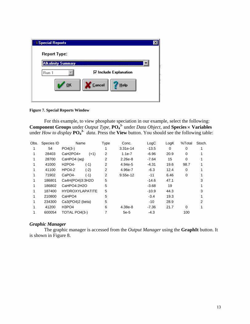
The Special Reports option contains seven text files that are produced as a result of extra calculations performed on the output data: (i) alkalinity report, (ii) total dissolved concentration report, (iii) total adsorbed concentration report, (iv) total dissolved minus total adsorbed concentration report, (v) ion balance report, (vi) saturation index report, (vii) summary report. To view a special report, first check the Special Report box, then click the View button. A new window titled Special Reports will appear (Figure 7). On the Special Reports window, you can use the combo box to select the text file you want to view.

13

Figure 7. Special Reports Window

For this example, to view phosphate speciation in our example, select the following:

Component Groups under Output Type, PO43- under Data Object, and Species × Variables

under How to display PO43- data. Press the View button. You should see the following table:

Obs. Species ID Name Type Conc. LogC LogK %Total Stoch.

1 54 PO4(3-) 1 3.31e-14 -13.5 0 0 1 1 28403 CaH2PO4+ (+1) 2 1.1e-7 -6.96 20.9 0 1 1 28700 CaHPO4 (aq) 2 2.26e-8 -7.64 15 0 1 1 41000 H2PO4- (-1) 2 4.94e-5 -4.31 19.6 98.7 1 1 41100 HPO4-2 (-2) 2 4.96e-7 -6.3 12.4 0 1 1 71902 CaPO4- (-1) 2 9.55e-12 -11 6.46 0 1 1 186801 Ca4H(PO4)3:3H2O 5 -14.6 47.1 3 1 186802 CaHPO4:2H2O 5 -3.68 19 1 1 187400 HYDROXYLAPATITE 5 -10.9 44.3 3 1 210800 CaHPO4 5 -3.4 19.3 1 1 234300 Ca3(PO4)2 (beta) 5 -10 28.9 2 1 41200 H3PO4 6 4.38e-8 -7.36 21.7 0 1 1 600054 TOTAL PO4(3-) 7 5e-5 -4.3 100

Graphic Manager

The graphic manager is accessed from the Output Manager using the GraphIt button. It is shown in Figure 8.

14

Figure 8. Graphic Manager Window There are five combo box buttons displayed on the screen:

The Graph Type lets you choose between Bar Chart and X-Y Plots. For single calculations you will only be able to choose a bar chart.

The Component box is a list of all of the components in this MDO. When you select a different component from this list the window on the right hand side of the screen will be updated to reflect the chemical species associated with that component. These species will comprise the y-axis for your plot.

The Observation box allows you to select which run you want to display for a bar chart. This option will not be active for X-Y Plots.

The Units box allows you to select the units for your y-axis. These can be the concentration, LogC, LogK, or %Total. This option will not be active when the bar chart is used.

The X-Axis box is a list of all of the variables that were included in your multirun file. This option will not be active when bar charts are chosen.

15

For this example, to plot the phosphate speciation, press GraphIt, type the graph title on the Graphics Manager window, select PO4

3- in Component box and Run 1 in Observation box. Press the Plot button. You should see the following Figure.

Figure 9. Graphic Output for Phosphate Speciation Saving Your Work

There are two ways to save input data for future MINEQL+ runs. First, you can save a complete problem set. This will store all of the reaction data, component totals, multirun data, and internal switches that were used to run the problem. To do so, just click the Save or SaveAs button from the File menu. A Windows tool will appear that will allow you to specify the name and location of the stored file. To retrieve the file later on, use the Open option in the File menu. Again, a Windows tool will appear that will help you to locate the file. If you make any changes to the thermodynamic data, these changes will also be saved. However, changes to the thermodynamic data will remain to the particular problem set, so if you want to use a new chemical species in a different problem set you would need to use the second approach, saving Personal Thermodynamic Data. This methods allow you save new reaction data or data that has been changed in some way. You can then retrieve that data for later use in any problem set. Example 2: Calculating equilibrium pH for closed and open systems

Exercise: I add 1 mg each of NaF, KCl, CaCO3 and Na2HPO4 salts to 1 liter of water. My aim is to find the pH and speciation of calcium in the water after taking ionic strength corrections into account assuming (i) a closed system (ii) an open system. How do I go about solving this problem using MINEQL+?

16

Answer: To answer (i), identify the basic individual components that make up the system. The basic individual components are the simplest forms of ions that can exist in a given solution. For the solution in the example, the basic components are Na+, K+, Ca(2+), H+, F-, Cl-, CO3(2-), PO4(3-) and either H2O or OH-. Next, select these components and press Scan THERMO to extract the reaction data you’ll need to run this problem. The reaction data for chemical species is stored in the default thermodynamics database and the Scan Thermo button tells MINEQL+ to extract only those reactions that are appropriate for the components you have selected.

The next screen that appears is the Tableau Tool for aqueous species. Aqueous species include dissolved complexes and ion pairs in solution. If we wanted to, we could add new species using the tableau tool or delete species that we didn’t want in the problem. For this problem, we will just review the data and accept the default configuration of species. Also, we’ll use the Totals Wizard to enter the concentrations of the individual components. Press the Close button. The Tableau Tool will disappear and a software tool (called Tableau Switch Tool) will appear that will allow you to look at other types of reaction data in your system. Select the species type you wish to view and press the Yes button to open the corresponding tableau. Once you are done viewing the species, press No in the Tableau Switch Tool to leave the Tableau Tool.

The Runtime Manager will open at this point. Switch ionic strength corrections to Calculated. We need to set the total molar concentrations of the different species for our system. Press the Wizard button located at the bottom of the RunTime Manager. The Totals Wizard will appear. At this point, you need to calculate the total concentrations of the individual species in molar units. Each salt dissociates completely to form the stoichiometric number of moles of counterions: [NaF]T = 0.001 g/L * 1 mole/41.99 g = 2.382 × 10-5 M [KCl]T = 0.001 g/L * 1 mole/74.5 g = 1.342 × 10-5 M [CaCO3]T = 0.001 g/L * 1 mole/100 g = 1.000 × 10-5 M [Na2HPO4]T = 0.001 g/L * 1 mole/142 g = 7.042 × 10-6 M The numbers shown in bold are the molecular weights of the salts. TOTNa = [NaF]T + 2 [Na2HPO4]T = 3.790 × 10-5 M TOTK = [KCl]T = 1.342 × 10-5 M TOTCl = [KCl]T = 1.342 × 10-5 M TOTCa = [CaCO3]T = 1.000 × 10-5 M TOTCO3 = [CaCO3]T = total carbonate in closed system. TOTF = [NaF]T = 2.382 x 10-5 M TOTPO4 = [Na2HPO4]T = 7.042 × 10-6 M

Enter the values for all the totals except carbonate. Now, use the mouse to press the tab labeled pH in the Calculation Wizard. Two buttons are located at the top of the pH Wizard: one labeled pH is supplied by user and another labeled pH is calculated by MINEQL+. In this scenario, since we want MINEQL+ to calculate the pH, we will use the option labeled pH is calculated by MINEQL+. Below these buttons, you’ll find three fields: one labeled pH value (which is inactive), the next Total H (M) and the last a check box with Base pH Calculation on Electroneutrality. Check this box in order to ask MINEQL to base it’s pH calculations on electroneutrality.

17

Next, use the mouse to press the tab labeled CO2 in the Calculation Wizard. At the top of the window are two buttons relating to the type of calculation that will be performed. Select the button labeled Closed to the Atmosphere. Next, move the mouse to the field labeled Total CO3 and type in the value 1e-5. Press the OK button at the top of the wizard to finalize your work. Now, you are ready to run your calculation. Specify a name for the output file. Press the Run button located at the bottom of the Runtime Manager.

After a second or two, the calculation will be completed and the Output Manager will appear. By default, the most recent type of output file is selected. Press the field labeled Special Reports under Output Type and then press the View button located at the bottom of the Output Manager. Under Report Type, choose the second option, viz. total dissolved concentrations by component. Listed here you will find the concentrations of all the basic components including the pH. The pH predicted by MINEQL+ is 8.802.

To examine calcium speciation, select the following: Ca2+ under Data Object, Component Groups under Output Type and Species × Variables under How to display Ca2+ data. Press the View button. You should see the following table: Obs.

Species ID Name

Type Conc.

LogC

LogK

%Total

Stoch.

1 16 Ca(2+) 15.75E-

06 -5.24 0 57.5 1

1 7300 CaOH+ (+1) 27.11E-

10 -9.15 -12.7 0 1

1 28400 CaHCO3+ (+1) 29.95E-

10 -9 11.6 0 1

1 28403 CaH2PO4+ (+1) 21.31E-

11 -10.9 20.9 0 1

1 28700 CaHPO4 (aq) 21.06E-

08 -7.97 15 0 1

1 71800 CaCO3 (aq) 22.49E-

09 -8.6 3.17 0 1

1 71900 CaF+ (+1) 21.44E-

09 -8.84 1.02 0 1

1 71902 CaPO4- (-1) 21.81E-

08 -7.74 6.41 0 1

1 187400 HYDROXYLAPATITE 48.43E-

07 0 44.1 42.1 51 186800 PORTLANDITE 5 -10.5 -22.8 11 186801 Ca4H(PO4)3:3H2O 5 -9.6 46.9 41 186802 CaHPO4:2H2O 5 -4.01 18.9 11 186700 LIME 5 -20.4 -32.7 11 210800 CaHPO4 5 -3.73 19.2 11 218800 ARAGONITE 5 -3.5 8.27 11 218900 CALCITE 5 -3.32 8.45 11 219400 FLUORITE 5 -4.01 10.5 11 234300 Ca3(PO4)2 (beta) 5 -4.75 28.8 3

1 600016 TOTAL Ca(2+) 75.79E-

06 -5.24 57.9

18

The table essentially shows the distribution of the total calcium in the system. Note that

57.5% of the calcium exists as free calcium ({Ca2+}= 5.75 × 10-6 M), and 42.1% of the calcium exists as hydroxyapatite. The sum of the calcium contained in Type I through V species adds up to the total calcium concentration in the system (1.00 × 10-5 M).

(ii) To answer question (ii), you need to alter the way in which total carbonate is entered in the Calculation Wizard. In this case, the second option i.e., Open to the Atmosphere is selected instead of the Closed to the Atmosphere option. Next, move the cursor to the field labeled Log PCO2. The PCO2 of CO2(g) at atmospheric pressure is 10-3.5. Since we are using a log value, we will need to input a value of –3.50 in this field. Press the OK button to finalize your work. You need not change the values in the Totals and pH fields of the Calculation Wizard. If you open the Tableau Tool for Fixed Entities, you’ll notice a species for CO2(g). You’ll also notice that the Log K value for this species is equal to 21.66. This value includes a correction for partial pressure. Close and return to the Runtime Manager. Change the name of the output file and press Run. Check to see how leaving a solution open to the atmosphere causes major changes in the speciation of the dissolved components. The pH of the solution in this case is 6.718.

Follow the steps outlined in part (i) of this example to obtain the speciation of calcium in an open system. You should obtain the following table: Obs.

Species ID

Name Type

Conc. LogC LogK %Total

Stoch.

1 16 Ca(2+) 1 9.98E-06 -5 0 99.8 11 7300 CaOH+ (+1) 2 1.01E-11 -11 -12.7 0 11 28400 CaHCO3+ (+1) 2 4.52E-09 -8.35 11.6 0 11 28403 CaH2PO4+ (+1) 2 1.12E-09 -8.95 20.9 0 11 28700 CaHPO4 (aq) 2 7.51E-09 -8.12 15 0 11 71800 CaCO3 (aq) 2 9.32E-11 -10 3.16 0 11 71900 CaF+ (+1) 2 2.49E-09 -8.6 1.02 0 11 71902 CaPO4- (-1) 2 1.05E-10 -9.98 6.4 0 11 186700 LIME 5 -24.3 -32.7 11 186800 PORTLANDITE 5 -14.4 -22.8 11 186801 Ca4H(PO4)3:3H2O 5 -14 46.9 41 186802 CaHPO4:2H2O 5 -4.17 18.9 11 187400 HYDROXYLAPATIT

E 5 -8.31 44.1 5

1 210800 CaHPO4 5 -3.88 19.2 11 218800 ARAGONITE 5 -4.93 8.26 11 218900 CALCITE 5 -4.75 8.44 11 219400 FLUORITE 5 -3.77 10.5 11 234300 Ca3(PO4)2 (beta) 5 -8.98 28.8 31 600016 TOTAL Ca(2+) 7 1.00E-05 -5 100

Notice that unlike in the closed system, almost all of the calcium in this case exists as

free calcium ({Ca2+}= 9.98 x 10-6 M). The speciation of calcium depends primarily on the pH. This will be evident after drawing a pC- pH diagram for calcium (using MINEQL+ to draw pC – pH diagrams is shown in the next example). A pC – pH diagram shows how the speciation of a compound changes with change in pH. At higher pH values, Ca2+ reacts with carbonate and

19

phosphate to form calcium carbonate and calcium phosphate. Hence, the concentration of free calcium in the solution is low. The opposite is true at low pHs. In our closed system example, the pH of the solution was 8.80. When the same system is opened to the atmosphere, carbonate from the atmosphere will be transferred to the water because the initial concentration of carbonate in the system is less than the equilibrium concentration of water open to the atmosphere. The pH of the solution decreases to 6.72 due to the hydrolysis of carbon dioxide to form the weak acid H2CO3. As the pH decreases, calcium carbonate and calcium phosphate dissociate to form free calcium. Thus, one notices an increase in the free calcium concentration for the open system. Example 3: Calculation of initial pH, total alkalinity; drawing pC – pH diagrams and performing synthetic titrations

Exercise: A container of water contains 5 mM NaT and 4 mM total carbonate. (i) What is the initial pH of the solution? (ii) What is the alkalinity of the solution? (iii) How does the speciation of the total carbonate in the solution change with respect to pH? (iv) How will the pH of the solution change when I add (titrate with) (a) a base (b) an acid? Take ionic strength corrections into effect while performing your calculations.

Answer: (i) Identify the basic components in the solution: Na+, H+, CO3(2-) and H2O/OH-. Select the components in the Component Selection Menu and scan the thermodynamic database. Go to the Runtime Manager and turn the ionic strength correction to Calculated. Next, go to the Wizard and enter the appropriate total sodium ion concentration in the Totals menu of the Calculation Wizard. Set the pH to be Calculated by MINEQL+ using the electroneutrality equation. In the CO2 field, make the system closed to the atmosphere and enter the total carbonate concentration under Total CO3 in molar units. Give a file name and run the calculation. The pH of the solution should be 9.688 (this can be seen under the Special Reports

View Total dissolved concentrations by component menu). (ii) For answering part (ii), the alkalinity of the sample can be read from the Alkalinity

Summary menu in the Report Type field of Special Reports. To get to this menu, select Special Reports under Output Type in the Output Manager and press the View button. The report will appear and you will see the pH on the left-hand side of the screen. You will notice that there are other values pertaining to the alkalinity of the system are also listed here. The total alkalinity of the solution should be 4.871 × 10-3 eq/L. Notice also that carbonate species contribute the most towards the alkalinity of the sample with a value of 4.818 × 10-3 eq/L.

(iii) One of the most common uses for MINEQL+ is examining the distribution of chemical species as a function of pH. MINEQL+ can automatically perform a series of calculations while changing the value of one variable. This gives us the possibility to examine chemical speciation along a defined and regularly-spaced pH interval. This calculation is referred to as a fixed pH titration. In MINEQL+, the word titration is used to refer to the change in any chemical parameter. So, as in the real world, it is possible to titrate with an acid or base, which we will do for answering part (iv) of this example.

To study the speciation of carbonate with respect to pH, select the components present in the system from the Select Components tool. The components are the same as in part (i) of the example. Scan the thermodynamic database; access the Calculation Wizard and input the total concentration values for Na+ and CO3(2-) in the totals and CO2 menus respectively. By default, the pH wizard should be configured to perform a fixed pH calculation and the calculation type

20

should be changed to pH is supplied by user (as opposed to pH is calculated by MINEQL+), used for parts (i) and (ii) of this example).

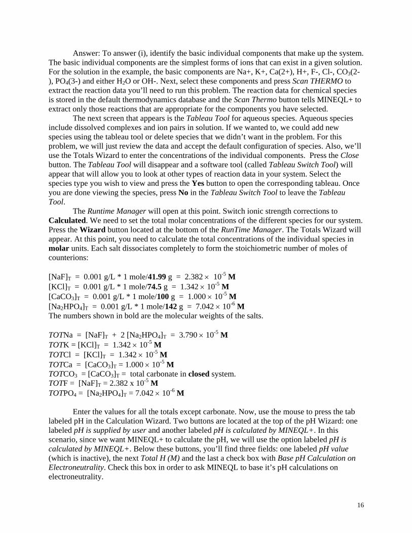
Figure 10. MultiRun Manager Window

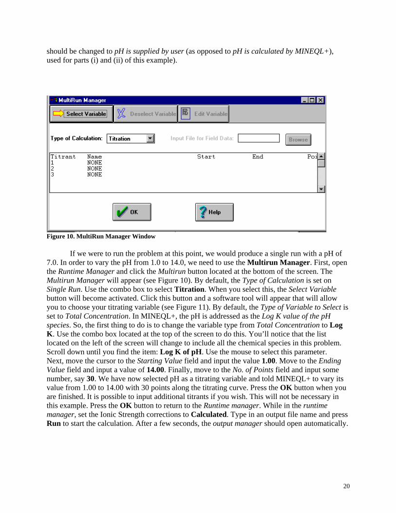
If we were to run the problem at this point, we would produce a single run with a pH of 7.0. In order to vary the pH from 1.0 to 14.0, we need to use the Multirun Manager. First, open the Runtime Manager and click the Multirun button located at the bottom of the screen. The Multirun Manager will appear (see Figure 10). By default, the Type of Calculation is set on Single Run. Use the combo box to select Titration. When you select this, the Select Variable button will become activated. Click this button and a software tool will appear that will allow you to choose your titrating variable (see Figure 11). By default, the Type of Variable to Select is set to Total Concentration. In MINEQL+, the pH is addressed as the Log K value of the pH species. So, the first thing to do is to change the variable type from Total Concentration to Log K. Use the combo box located at the top of the screen to do this. You’ll notice that the list located on the left of the screen will change to include all the chemical species in this problem. Scroll down until you find the item: Log K of pH. Use the mouse to select this parameter. Next, move the cursor to the Starting Value field and input the value 1.00. Move to the Ending Value field and input a value of 14.00. Finally, move to the No. of Points field and input some number, say 30. We have now selected pH as a titrating variable and told MINEQL+ to vary its value from 1.00 to 14.00 with 30 points along the titrating curve. Press the OK button when you are finished. It is possible to input additional titrants if you wish. This will not be necessary in this example. Press the OK button to return to the Runtime manager. While in the runtime manager, set the Ionic Strength corrections to Calculated. Type in an output file name and press Run to start the calculation. After a few seconds, the output manager should open automatically.

21

Figure 11. Selecting Variables for MultiRun

From within the Output Manager, click the GraphIT button to open the Graphics Manager. Move the cursor to the combo box labeled Component and select CO3(2-). The list on the right-hand side will be updated to reflect the carbonate species included in this problem. Choose the species that you wish to view. You may choose all the species if you wish. Make sure that the units are set to Log C. Press the Plot button to produce the log C-pH diagram for carbonate species (Figure 12).

Figure 12: Speciation of carbonate species in a closed system. At low pHs, H2CO3 is the major form of carbonate while at high pHs, CO3

2- is the dominant species. At intermediate pHs, the bicarbonate form (HCO3-) is

dominant. Other species are present, albeit at lower concentrations.

22

(iv) To answer part (iii), we varied the pH along pre-determined fixed values. For answering part (iv), we will allow MINEQL+ to calculate the pH using information about the ion balance in the system. While performing titrations, we will vary the concentration of some species that is not present in the original system and study the effect of adding that variable on the pH of the system. Thus, for our system, for base titration, one can use KOH if K+ is not present in the system, while for acid titration, one can use HCl or H2SO4 if Cl- or SO4

2- are not present in the system. In this example, we will carry out a titration with the acid HCl.

In addition to H2O, H+, CO3(2-) and Na+, select Cl- from the Select Components tool. Scan the thermodynamic database. Open the Calculation Wizard and set the concentration for Na+ to 5.0E-3 and the concentration of CO3(2-) to 4.0E-3 in the totals and CO2 menus respectively. Note that you can leave the value for Cl- at 0 since you will be using Cl- as your titrating variable. Next, go to the pH wizard and make sure the Calculation Type is set to pH is calculated by MINEQL+. Also, make sure the check box is selected to base pH calculation on Electroneutrality. Press the OK button at the top of the screen to finalize your work. Open the Runtime Manager and access the multirun features by pressing the Multirun button at the bottom of the screen. Change the Type of Calculation to Titration. The Select variable option will become activated. Press this button and a tool will appear that will allow you to set the information for your titrating variable. Although we are trying to simulate a titration with HCl, it is not necessary to vary both H+ and Cl-. Since we have told MINEQL+ to calculate the pH based on electroneutrality, the total H+ concentration will be determined by the electroneutrality equation. As a result, we only need to be concerned with the concentration of total Cl-.

Select Total Conc. of Cl- from the list on the left-hand side of the screen. Move the cursor to the Starting Value field and input a value close to zero, say, 1.0E-10 (in molar units). Next, input a value higher than the alkalinity of the original system, say, 7.0E-3. Finally, set the No. of points to 25. Press OK when you are done to return to the Multirun Manager. Press the OK button again to return to the Runtime Manager. In the Ionic Strength Corrections section, select the Calculated button. Set the output name and press the Run button at the bottom of the screen to start the calculation.

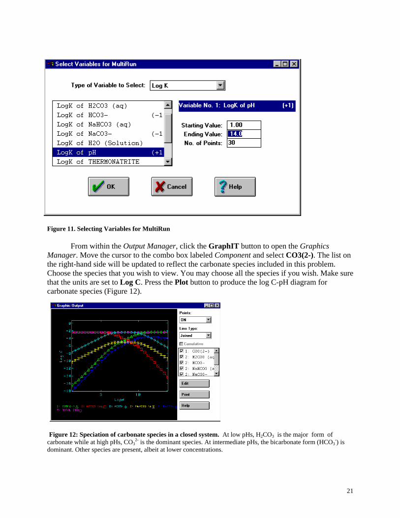
Open the output manager and press the GraphIT button at the bottom of the screen. The Graphics manager will be displayed. We are interested in plotting pH versus moles of acid added. To do this, select H(+) from the composition combo box. Then, for the y-axis, select 1: H(+) from the list on the right-hand side of the screen. Make sure that the units field is set to Log C. Press the Plot button at the bottom of the screen to generate the graph. This will display a plot of the Log {H+} vs Cl- added (Figure 13).

23

Figure 13: Titration curve – Log{H+} versus volume of acid (HCl) added. When the concentration of Cl- changes from 0.0015 M to 0.004 M, the pH of the system is stable at a value of around 6.3. The solution is well-buffered in this region because the pH changes little for large acid additions. The central pH value in this region of the diagram is the pKa of the solution. Such a diagram for a natural water sample may exhibit multiple pKas because natural waters can contain more than one acid or base, or multiprotic acids. Note: Other special reports of interest are the sixth and seventh options in Special Reports, which deal with the saturation index report and summary of all species in a single run, respectively. The reported saturation index is computed as:

Saturation Index, SI = log (Q/Ksp) Where Q is the ion product and Ksp is the solubility constant for the solid. Example: CaCO3 (S) Ca2+ + CO3

2- Reaction Quotient = Q = {Ca2+}{CO3

2-} A negative SI implies undersaturation of the solution with respect to CaCO3(s); zero implies an equilibrium (saturation point); a positive value implies oversaturation. The seventh option simply lists the concentrations of all possible species/complexes in the solution including the pH of the solution. Also listed is the type of species viz. Type I, II, etc.

24

Example 4: Saturation Index Computations (SI) Exercise: 1 nanomole of Fe(OH)3 is added to 1 liter of water at room temperature.

Determine if any solids are formed. Answer: The solubility of Fe3+ in water is very low. Hence, some solids will be formed in

the solution. Select Fe3+, H+ and H2O from the Component Selection menu and scan the

thermodynamics database. Move all the solids from Type V (dissolved solids) to Type VI (Species not considered) to view the SI’s of all solids. Go to the Wizard and enter the appropriate total ferric iron concentration in the Totals menu. Set the pH to 7.00. Run the calculation.

To view the saturation indices, click on Special Reports under output type and choose the sixth option: saturation index report. The report should contain the following numbers for the saturation index: Lepidocrocite Goethite Hematite Ferrihydrite Maghemite 1.178 2.058 6.516 -0.642 -1.288 This report shows that the solution is oversaturated with respect to Lepidocrocite, Goethite, and Hematite. The solution is undersaturated with respect to Ferrihydrite and Maghemite.