C H A P T E R 8 -...

Copyright © 2013 Pearson Education, Inc. • Microeconomics • Pindyck/Rubinfeld, 8e. 1 of 35

8.1 Perfectly Competitive Markets

8.2 Profit maximization

8.3 Marginal Revenue, Marginal

Cost, and Profit Maximization

8.4 Choosing Output in the Short

Run

8.5 The Competitive Firm’s Short-

Run Supply Curve

8.6 The Short-Run Market Supply

Curve

8.7 Choosing Output in the Long-Run

8.8 The Industry’s Long-Run Supply

Curve

C H A P T E R 8

Prepared by:

Fernando Quijano, Illustrator

Profit Maximization

and Competitive Supply CHAPTER OUTLINE

2 of 35 Copyright © 2013 Pearson Education, Inc. • Microeconomics • Pindyck/Rubinfeld, 8e.

Perfectly Competitive Markets 8.1

PRICE TAKING

Because each individual firm sells a sufficiently small proportion of total market

output, its decisions have no impact on market price.

● price taker Firm that has no influence over market price and thus takes the

price as given.

PRODUCT HOMOGENEITY

When the products of all of the firms in a market are perfectly substitutable with

one another—that is, when they are homogeneous—no firm can raise the price

of its product above the price of other firms without losing most or all of its

business.

In contrast, when products are heterogeneous, each firm has the opportunity to

raise its price above that of its competitors without losing all of its sales.

The assumption of product homogeneity is important because it ensures that

there is a single market price, consistent with supply-demand analysis.


FREE ENTRY AND EXIT

● free entry (or exit) Condition under which there are no special

costs that make it difficult for a firm to enter (or exit) an industry.

When Is a Market Highly Competitive?

Many markets are highly competitive in the sense that firms face highly elastic

demand curves and relatively easy entry and exit. But there is no simple rule of

thumb to describe whether a market is close to being perfectly competitive.

Because firms can implicitly or explicitly collude in setting prices, the presence of

many firms is not sufficient for an industry to approximate perfect competition.

Conversely, the presence of only a few firms in a market does not rule out

competitive behavior.

With free entry and exit, buyers can easily switch from one supplier to another,

and suppliers can easily enter or exit a market.


Profit Maximization 8.2

Do Firms Maximize Profit?

The assumption of profit maximization is frequently used in microeconomics

because it predicts business behavior reasonably accurately and avoids

unnecessary analytical complications.

For smaller firms managed by their owners, profit is likely to dominate almost

all decisions. In larger firms, however, managers who make day-to-day

decisions usually have little contact with the owners.

Firms that do not come close to maximizing profit are not likely to survive. The

firms that do survive make long-run profit maximization one of their highest

priorities.

Alternative Forms of Organization

● cooperative Association of businesses or people jointly owned and

operated by members for mutual benefit.

● condominium A housing unit that is individually owned but provides

access to common facilities that are paid for and controlled jointly by an

association of owners.


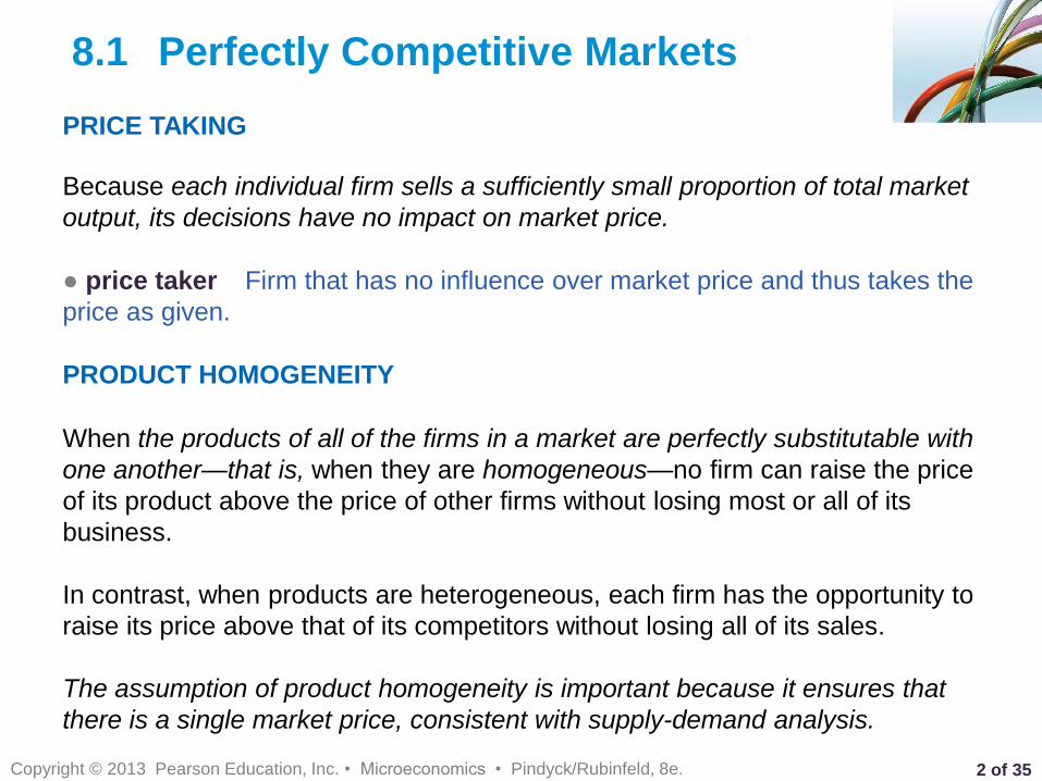
While owners of condominiums must join with fellow condo owners to manage

common, they can make their own decisions as to how to manage their

individual units. In contrast, co-ops share joint liability on any outstanding

mortgage on the co-op building and are subject to more complex governance

rules.

Nationwide, condos are far more common than co-ops, outnumbering them by

a factor of nearly 10 to 1. In this regard, New York City is very different from the

rest of the nation—co-ops are more popular, and outnumber condos by a factor

of about 4 to 1.

Many building restrictions in New York have long disappeared, and yet the

conversion of apartments from co-ops to condos has been relatively slow.

The typical condominium apartment is worth about 15.5 percent more than a

equivalent apartment held in the form of a co-op. Clearly, holding an apartment

in the form of a co-op is not the best way to maximize the apartment’s value.

It appears that in New York, many owners have been willing to forgo

substantial amounts of money in order to achieve non-monetary benefits.

EXAMPLE 8.1 CONDOMINIUMS VERSUS COOPERATIVES IN

NEW YORK CITY


Marginal Revenue, Marginal Cost,

and Profit Maximization

8.3

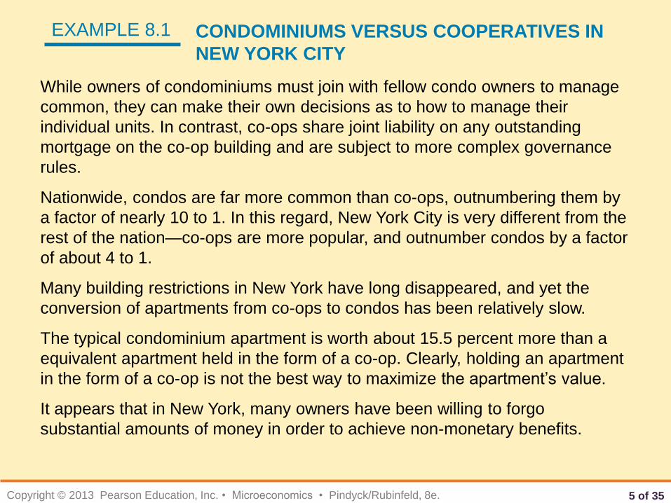
● profit Difference between total revenue and total cost.

π(q) = R(q) − C(q)

● marginal revenue Change in revenue resulting from a one-unit increase in

output.

A firm chooses output q*, so that

profit, the difference AB between

revenue R and cost C, is

maximized.

At that output, marginal revenue

(the slope of the revenue curve) is

equal to marginal cost (the slope

of the cost curve).

Δπ/Δq = ΔR/Δq − ΔC/Δq = 0

MR(q) = MC(q)

PROFIT MAXIMIZATON IN

THE SHORT RUN

FIGURE 8.1


Demand and Marginal Revenue for a Competitive Firm

A competitive firm supplies only a small portion of the total output of all the firms in an

industry. Therefore, the firm takes the market price of the product as given, choosing

its output on the assumption that the price will be unaffected by the output choice.

In (a) the demand curve facing the firm is perfectly elastic,

even though the market demand curve in (b) is downward sloping.

DEMAND CURVE FACED BY A COMPETITIVE FIRM

FIGURE 8.2


The demand curve d facing an individual firm in a competitive market is

both its average revenue curve and its marginal revenue curve. Along this

demand curve, marginal revenue, average revenue, and price are all equal.

Profit Maximization by a Competitive Firm

MC(q) = MR = P

Because each firm in a competitive industry sells only a small fraction

of the entire industry output, how much output the firm decides to sell

will have no effect on the market price of the product.

Because it is a price taker, the demand curve d facing an individual competitive

firm is given by a horizontal line.

A perfectly competitive firm should choose its output so that marginal cost

equals price:


Short-Run Profit Maximization by a Competitive Firm

A COMPETITIVE FIRM

MAKING A POSITIVE

PROFIT

FIGURE 8.3

In the short run, the

competitive firm maximizes

its profit by choosing an

output q* at which its

marginal cost MC is equal

to the price P (or marginal

revenue MR) of its product.

The profit of the firm is

measured by the rectangle

ABCD.

Any change in output,

whether lower at q1 or

higher at q2, will lead to

lower profit. Output Rule: If a firm is producing any

output, it should produce at the level at which

marginal revenue equals marginal cost.

Choosing Output in the Short Run 8.4


When Should the Firm Shut Down?

A COMPETITIVE FIRM

INCURRING LOSSES

FIGURE 8.4

A competitive firm should

shut down if price is below

AVC.

The firm may produce in

the short run if price is

greater than average

variable cost.


THE SHORT-RUN OUTPUT OF AN

ALUMINUM SMELTING PLANT

FIGURE 8.5

EXAMPLE 8.2 THE SHORT-RUN OUTPUT DECISION OF AN

ALUMINUM SMELTING PLANT

How should the manager determine the plant’s profit maximizing

output? Recall that the smelting plant’s short-run marginal cost of

production depends on whether it is running two or three shifts

per day.

In the short run, the plant should

produce 600 tons per day if price is

above $1140 per ton but less than

$1300 per ton.

If price is greater than $1300 per

ton, it should run an overtime shift

and produce 900 tons per day.

If price drops below $1140 per ton,

the firm should stop producing, but

it should probably stay in business

because the price may rise in the

future.


The application of the rule that marginal revenue should equal marginal cost

depends on a manager’s ability to estimate marginal cost. First, except under

limited circumstances, average variable cost should not be used as a substitute

for marginal cost.

EXAMPLE 8.3 SOME COST CONSIDERATIONS FOR MANAGERS

Current output 100 units per day, 80 of which are produced during the regular shift and

20 of which are produced during overtime

Materials cost $8 per unit for all output

Labor cost $30 per unit for the regular shift; $50 per unit for the overtime shift

For the first 80 units of output, average variable cost and marginal cost are both

equal to $38 per unit. When output increases to 100 units, marginal cost is

higher than average variable cost, so a manager who relies on average

variable cost will produce too much.

Also, a single item on a firm’s accounting ledger may have two components,

only one of which involves marginal cost.

Finally, all opportunity costs should be included in determining marginal cost.

These three guidelines can help a manager to measure marginal cost correctly.

Failure to do so can cause production to be too high or too low and thereby

reduce profit.


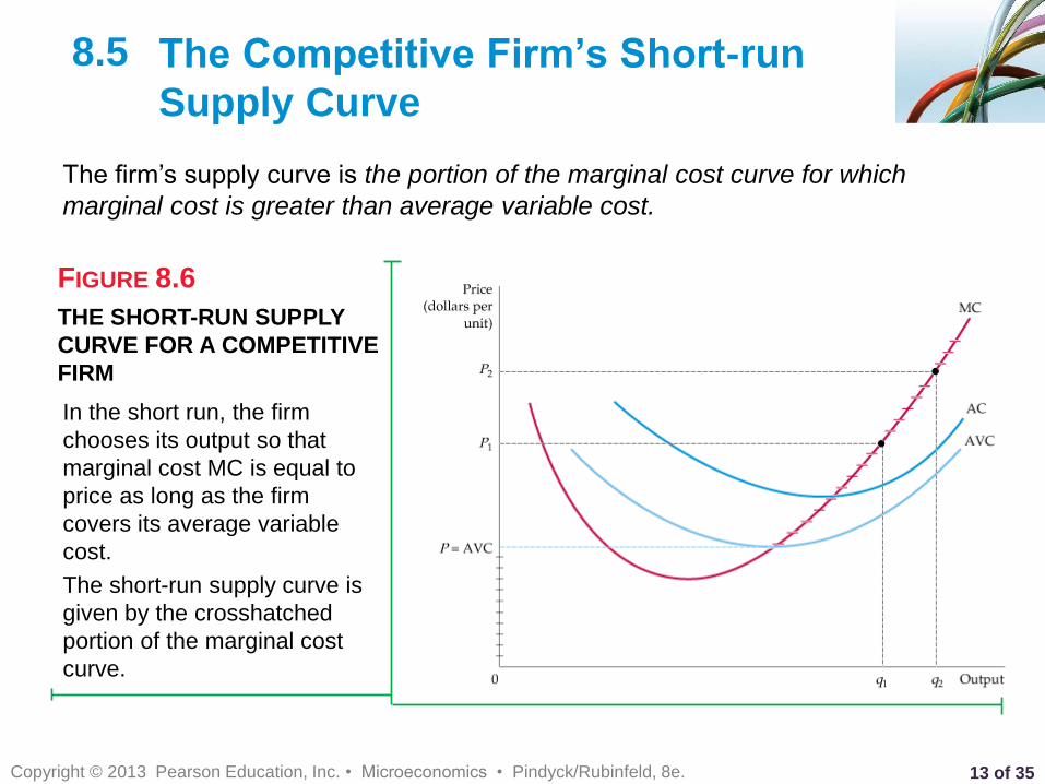
The Competitive Firm’s Short-run

Supply Curve

8.5

THE SHORT-RUN SUPPLY

CURVE FOR A COMPETITIVE

FIRM

FIGURE 8.6

The firm’s supply curve is the portion of the marginal cost curve for which

marginal cost is greater than average variable cost.

In the short run, the firm

chooses its output so that

marginal cost MC is equal to

price as long as the firm

covers its average variable

cost.

The short-run supply curve is

given by the crosshatched

portion of the marginal cost

curve.


THE RESPONSE OF A FIRM

TO A CHANGE IN INPUT

PRICE

FIGURE 8.7

When the marginal cost of

production for a firm

increases (from MC1 to MC2),

the level of output that

maximizes profit falls (from q1

to q2).

The Firm’s Response to an Input Price Change


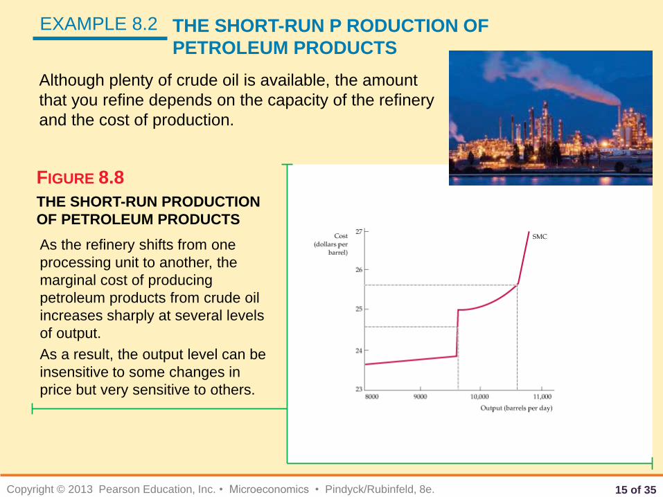
THE SHORT-RUN PRODUCTION

OF PETROLEUM PRODUCTS

FIGURE 8.8

EXAMPLE 8.2 THE SHORT-RUN P RODUCTION OF

PETROLEUM PRODUCTS

Although plenty of crude oil is available, the amount

that you refine depends on the capacity of the refinery

and the cost of production.

As the refinery shifts from one

processing unit to another, the

marginal cost of producing

petroleum products from crude oil

increases sharply at several levels

of output.

As a result, the output level can be

insensitive to some changes in

price but very sensitive to others.


The Short-Run Market Supply Curve 8.6

INDUSTRY SUPPLY IN THE

SHORT RUN

FIGURE 8.9

The short-run industry

supply curve is the

summation of the supply

curves of the individual

firms.

Because the third firm has

a lower average variable

cost curve than the first two

firms, the market supply

curve S begins at price P1

and follows the marginal

cost curve of the third firm

MC3 until price equals P2,

when there is a kink.

For P2 and all prices above

it, the industry quantity

supplied is the sum of the

quantities supplied by each

of the three firms.

Elasticity of Market Supply

Es = (ΔQ/Q)/(ΔP/P)


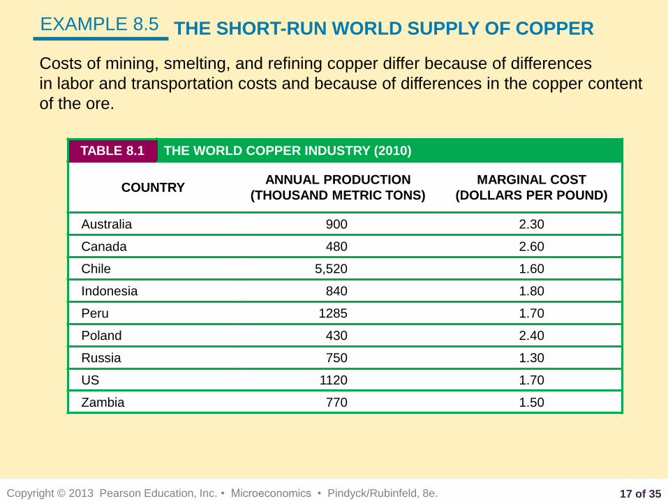
EXAMPLE 8.5 THE SHORT-RUN WORLD SUPPLY OF COPPER

Costs of mining, smelting, and refining copper differ because of differences

in labor and transportation costs and because of differences in the copper content

of the ore.

TABLE 8.1 THE WORLD COPPER INDUSTRY (2010)

COUNTRY ANNUAL PRODUCTION

(THOUSAND METRIC TONS)

MARGINAL COST

(DOLLARS PER POUND)

Australia 900 2.30

Canada 480 2.60

Chile 5,520 1.60

Indonesia 840 1.80

Peru 1285 1.70

Poland 430 2.40

Russia 750 1.30

US 1120 1.70

Zambia 770 1.50


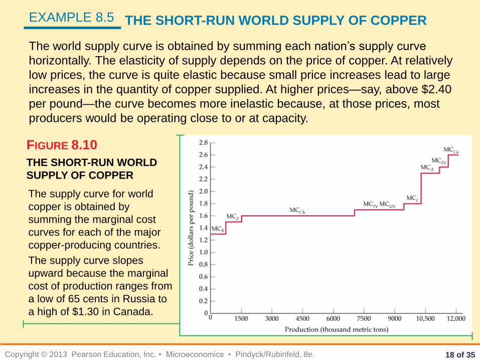
THE SHORT-RUN WORLD

SUPPLY OF COPPER

FIGURE 8.10

EXAMPLE 8.5 THE SHORT-RUN WORLD SUPPLY OF COPPER

The world supply curve is obtained by summing each nation’s supply curve

horizontally. The elasticity of supply depends on the price of copper. At relatively

low prices, the curve is quite elastic because small price increases lead to large

increases in the quantity of copper supplied. At higher prices—say, above $2.40

per pound—the curve becomes more inelastic because, at those prices, most

producers would be operating close to or at capacity.

The supply curve for world

copper is obtained by

summing the marginal cost

curves for each of the major

copper-producing countries.

The supply curve slopes

upward because the marginal

cost of production ranges from

a low of 65 cents in Russia to

a high of $1.30 in Canada.


Producer Surplus in the Short Run

● producer surplus Sum over all units produced by a firm of

differences between the market price of a good and the marginal cost of

production.

PRODUCER SURPLUS FOR

A FIRM

FIGURE 8.11

The producer surplus for a

firm is measured by the

yellow area below the market

price and above the marginal

cost curve, between outputs 0

and q*, the profit-maximizing

output.

Alternatively, it is equal to

rectangle ABCD because the

sum of all marginal costs up

to q* is equal to the variable

costs of producing q*.


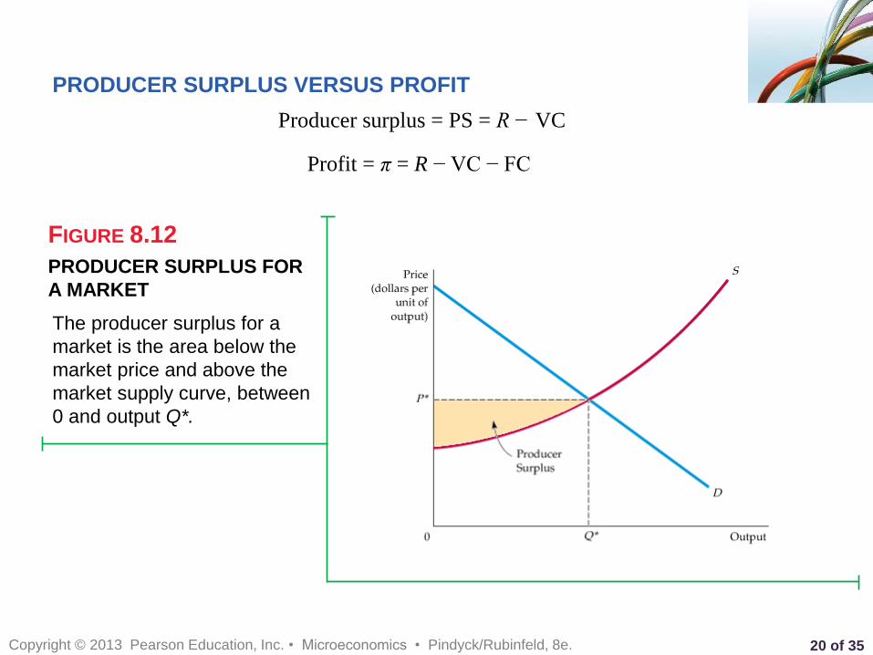
PRODUCER SURPLUS VERSUS PROFIT

PRODUCER SURPLUS FOR

A MARKET

FIGURE 8.12

Producer surplus = PS = R − VC

Profit = π = R − VC − FC

The producer surplus for a

market is the area below the

market price and above the

market supply curve, between

0 and output Q*.


Long-Run Profit Maximization

OUTPUT CHOICE IN THE

LONG RUN

FIGURE 8.13

The firm maximizes its profit

by choosing the output at

which price equals long-run

marginal cost LMC.

In the diagram, the firm

increases its profit from

ABCD to EFGD by

increasing its output in the

long run.

The long-run output of a profit-maximizing competitive firm is the point at which

long-run marginal cost equals the price.

Choosing Output in the Long Run 8.7


Long-Run Competitive Equilibrium

ACCOUNTING PROFIT AND ECONOMIC PROFIT

π = R − wL − rK

ZERO ECONOMIC PROFIT

● zero economic profit A firm is earning a normal return on its investment—

i.e., it is doing as well as it could by investing its money elsewhere.

ENTRY AND EXIT

In a market with entry and exit, a firm enters when it can earn a positive long-

run profit and exits when it faces the prospect of a long-run loss.

Economic profit takes into account opportunity costs. One such opportunity cost

is the return to the firm’s owners if their capital were used elsewhere. Accounting

profit equals revenues R minus labor cost wL, which is positive. Economic profit

𝜋, however, equals revenues R minus labor cost wL minus the capital cost, Rk.


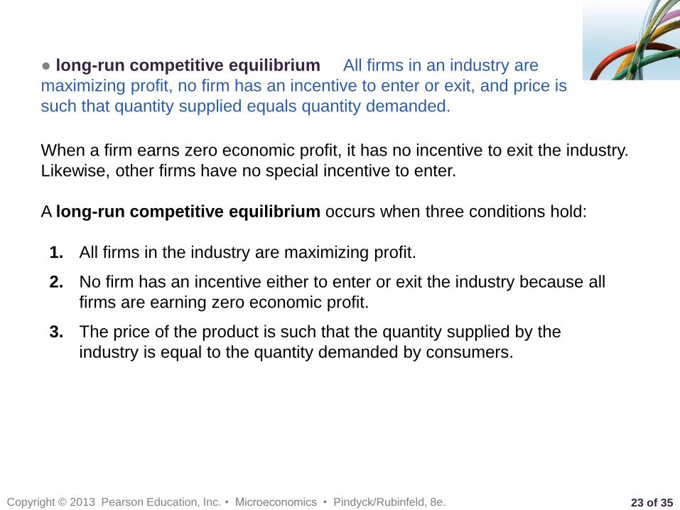
● long-run competitive equilibrium All firms in an industry are

maximizing profit, no firm has an incentive to enter or exit, and price is

such that quantity supplied equals quantity demanded.

When a firm earns zero economic profit, it has no incentive to exit the industry.

Likewise, other firms have no special incentive to enter.

A long-run competitive equilibrium occurs when three conditions hold:

1. All firms in the industry are maximizing profit.

2. No firm has an incentive either to enter or exit the industry because all

firms are earning zero economic profit.

3. The price of the product is such that the quantity supplied by the

industry is equal to the quantity demanded by consumers.


LONG-RUN COMPETITIVE

EQUILIBRIUM

FIGURE 8.14

Initially the long-run equilibrium

price of a product is $40 per unit,

shown in (b) as the intersection of

demand curve D and supply curve

S1.

In (a) we see that firms earn

positive profits because long-run

average cost reaches a minimum

of $30 (at q2).

Positive profit encourages entry of

new firms and causes a shift to

the right in the supply curve to S2,

as shown in (b).

The long-run equilibrium occurs at

a price of $30, as shown in (a),

where each firm earns zero profit

and there is no incentive to enter

or exit the industry.


FIRMS HAVING IDENTICAL COSTS

To see why all the conditions for long-run equilibrium must hold,

assume that all firms have identical costs.

Now consider what happens if too many firms enter the industry in

response to an opportunity for profit. The industry supply curve will shift

further to the right, and price will fall.

Only when there is no incentive to exit or enter can a market be in long-

run equilibrium.

FIRMS HAVING DIFFERENT COSTS

Now suppose that all firms in the industry do not have identical cost curves.

Perhaps one firm has a patent that lets it produce at a lower average cost than

all the others. In that case, it is consistent with long-run equilibrium for that firm

to earn a greater accounting profit and to enjoy a higher producer surplus than

other firms.

If the patent is profitable, other firms in the industry will pay to use it. The

increased value of the patent thus represents an opportunity cost to the firm

that holds it. It could sell the rights to the patent rather than use it. If all firms

are equally efficient otherwise, the economic profit of the firm falls to zero.


THE OPPORTUNITY COST OF LAND

There are other instances in which firms earning positive accounting profit may

be earning zero economic profit.

Suppose, for example, that a clothing store happens to be located near a large

shopping center. The additional flow of customers can substantially increase

the store’s accounting profit because the cost of the land is based on its

historical cost. When the opportunity cost of land is included, the profitability of

the clothing store is no higher than that of its competitors.

Economic Rent

In competitive markets, in both the short and the long run, economic rent is

often positive even though profit is zero.

● economic rent Amount that firms are willing to pay for an input less the

minimum amount necessary to obtain it.

In the long run, in a competitive market, the producer surplus that a firm earns

on the output that it sells consists of the economic rent that it enjoys from all its

scarce inputs.

Producer Surplus in the Long Run


FIRMS EARN ZERO PROFIT IN LONG-RUN EQUILIBRIUM

FIGURE 8.15

In long-run equilibrium, all firms earn zero economic profit.

In (a), a baseball team in a moderate-sized city sells enough tickets so that price ($7) is

equal to marginal and average cost.

In (b), the demand is greater, so a $10 price can be charged. The team increases sales

to the point at which the average cost of production plus the average economic rent is

equal to the ticket price.

When the opportunity cost associated with owning the franchise is taken into account,

the team earns zero economic profit.


The Industry’s Long-Run Supply Curve 8.8 Constant-Cost Industry

● constant-cost industry Industry whose long-run supply curve is horizontal.

In (b), the long-run supply

curve in a constant-cost

industry is a horizontal line SL.

When demand increases,

initially causing a price rise,

the firm initially increases its

output from q1 to q2, as shown

in (a).

But the entry of new firms

causes a shift to the right in

industry supply.

Because input prices are

unaffected by the increased

output of the industry, entry

occurs until the original price is

obtained (at point B in (b)).

The long-run supply curve for a constant-cost industry is,

therefore, a horizontal line at a price that is equal to the

long-run minimum average cost of production.

LONG-RUN SUPPLY IN A

CONSTANT COST INDUSTRY

FIGURE 8.16


The Industry’s Long-Run Supply Curve 8.8 Increasing-Cost Industry

● increasing-cost industry Industry whose long-run supply curve is upward sloping.

LONG-RUN SUPPLY IN AN

INCREASING COST INDUSTRY

FIGURE 8.17

In (b), the long-run supply

curve in an increasing-cost

industry is an upward-sloping

curve SL.

When demand increases,

initially causing a price rise,

the firms increase their output

from q1 to q2 in (a).

In that case, the entry of new

firms causes a shift to the right

in supply from S1 to S2.

Because input prices increase

as a result, the new long-run

equilibrium occurs at a higher

price than the initial

equilibrium.

In an increasing-cost industry, the long-run

industry supply curve is upward sloping.


Decreasing-Cost Industry

● decreasing-cost industry Industry whose long-run supply curve is

downward sloping.

You have been introduced to industries that have constant, increasing, and

decreasing long-run costs.

We saw that the supply of coffee is extremely elastic in the long run. The

reason is that land for growing coffee is widely available and the costs of

planting and caring for trees remains constant as the volume grows. Thus,

coffee is a constant-cost industry.

The oil industry is an increasing cost industry because there is a limited

availability of easily accessible, large-volume oil fields.

Finally, a decreasing-cost industry. In the automobile industry, certain cost

advantages arise because inputs can be acquired more cheaply as the volume

of production increases.

EXAMPLE 8.6 CONSTANT-, INCREASING-, AND DECREASING-COST

INDUSTRIES: COFFEE, OIL, AND AUTOMOBILES


The Effects of a Tax

An output tax raises the firm’s

marginal cost curve by the

amount of the tax.

The firm will reduce its output

to the point at which the

marginal cost plus the tax is

equal to the price of the

product.

EFFECT OF AN OUTPUT TAX

ON A COMPETITIVE FIRM’S

OUTPUT

FIGURE 8.18


EFFECT OF AN OUTPUT TAX

ON INDUSTRY OUTPUT

FIGURE 8.19

An output tax placed on all

firms in a competitive market

shifts the supply curve for the

industry upward by the

amount of the tax.

This shift raises the market

price of the product and

lowers the total output of the

industry.


Long-Run Elasticity of Supply

The long-run elasticity of industry supply is defined in the same way as

the short-run elasticity: It is the percentage change in output (Q/Q) that

results from a percentage change in price (P/P).

In a constant-cost industry, the long-run supply curve is horizontal, and the

long-run supply elasticity is infinitely large. (A small increase in price will induce

an extremely large increase in output.) In an increasing-cost industry, however,

the long-run supply elasticity will be positive but finite.

Because industries can adjust and expand in the long run, we would generally

expect long-run elasticities of supply to be larger than short-run elasticities.

The magnitude of the elasticity will depend on the extent to which input costs

increase as the market expands. For example, an industry that depends on

inputs that are widely available will have a more elastic long-run supply than

will an industry that uses inputs in short supply.


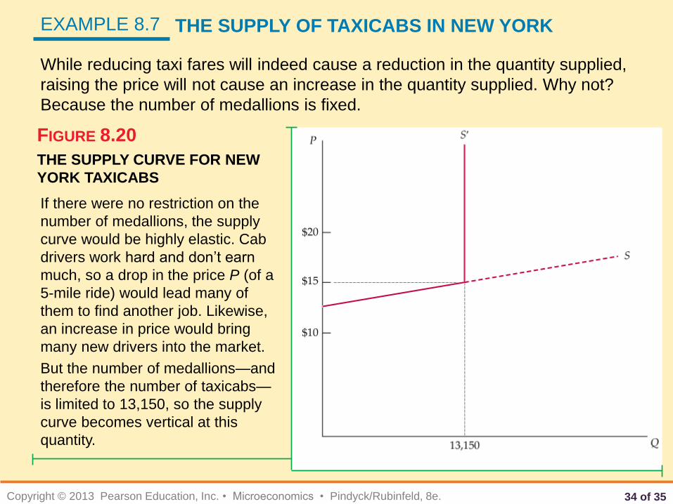
THE SUPPLY CURVE FOR NEW

YORK TAXICABS

FIGURE 8.20

EXAMPLE 8.7 THE SUPPLY OF TAXICABS IN NEW YORK

While reducing taxi fares will indeed cause a reduction in the quantity supplied,

raising the price will not cause an increase in the quantity supplied. Why not?

Because the number of medallions is fixed.

If there were no restriction on the

number of medallions, the supply

curve would be highly elastic. Cab

drivers work hard and don’t earn

much, so a drop in the price P (of a

5-mile ride) would lead many of

them to find another job. Likewise,

an increase in price would bring

many new drivers into the market.

But the number of medallions—and

therefore the number of taxicabs—

is limited to 13,150, so the supply

curve becomes vertical at this

quantity.


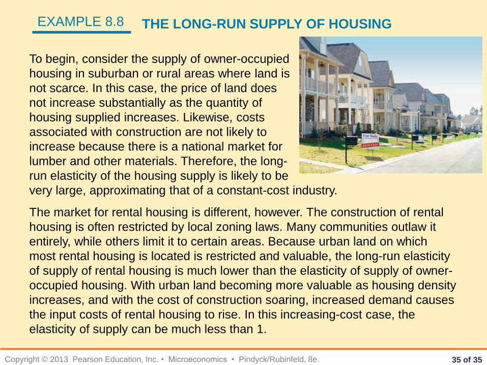
To begin, consider the supply of owner-occupied

housing in suburban or rural areas where land is

not scarce. In this case, the price of land does

not increase substantially as the quantity of

housing supplied increases. Likewise, costs

associated with construction are not likely to

increase because there is a national market for

lumber and other materials. Therefore, the long-

run elasticity of the housing supply is likely to be

very large, approximating that of a constant-cost industry.

The market for rental housing is different, however. The construction of rental

housing is often restricted by local zoning laws. Many communities outlaw it

entirely, while others limit it to certain areas. Because urban land on which

most rental housing is located is restricted and valuable, the long-run elasticity

of supply of rental housing is much lower than the elasticity of supply of owner-

occupied housing. With urban land becoming more valuable as housing density

increases, and with the cost of construction soaring, increased demand causes

the input costs of rental housing to rise. In this increasing-cost case, the

elasticity of supply can be much less than 1.

EXAMPLE 8.8 THE LONG-RUN SUPPLY OF HOUSING

C H A P T E R 8 -...

Documents

Transcript of C H A P T E R 8 -...