°c All rights reserved - NCSU

Two-Window Heterodyne Methods to Characterize Light

Fields

by

Frank Reil

Department of PhysicsDuke University

Date:Approved:

Dr. John E. Thomas, Supervisor

Dr. Daniel J. Gauthier

Dr. Robert Behringer

Dr. Moo-Young Han

Dr. Bob Guenther

Dissertation submitted in partial fulfillment of therequirements for the degree of Doctor of Philosophy

in the Department of Physicsin the Graduate School of

Duke University

2003

abstract

(Physics)

Two-Window Heterodyne Methods to Characterize Light

Fields

by

Frank Reil

Department of PhysicsDuke University

Date:Approved:

Dr. John E. Thomas, Supervisor

Dr. Daniel J. Gauthier

Dr. Robert Behringer

Dr. Moo-Young Han

Dr. Bob Guenther

An abstract of a dissertation submitted in partial fulfillment ofthe requirements for the degree of Doctor of Philosophy

in the Department of Physicsin the Graduate School of

Duke University

2003

Abstract

In this dissertation, I develop a novel Two-Window heterodyne technique for mea-

suring the time-resolved Wigner function of light fields, which allows their complete

characterization. A Wigner function is a quasi-probability density that describes

the transverse position and transverse momentum of a light field and is Fourier-

transform related to its mutual coherence function. It obeys rigorous transport

equations and therefore provides an ideal way to characterize a light field and

its propagation through various media. I first present the experimental setup of

our Two-Window technique, which is based on a heterodyne scheme involving two

phase-coupled Local Oscillator beams we call the Dual-LO. The Dual-LO consists

of a focused beam (’SLO’) which sets the spatial resolution, and a collimated beam

(’BLO’) which sets the momental resolution. The resolution in transverse posi-

tion and transverse momentum can be adjusted individually by the size of the

SLO and BLO, which enables a measurement resolution surpassing the uncertainty

principle associated with Fourier-transform pairs which limits the resolution when

just a single LO is used. We first use our technique to determine the beam size,

transverse coherence length and radius of curvature of a Gaussian-Schell beam, as

well as its longitudinal characteristics, which are related to its optical spectrum.

We then examine Enhanced Backscattering at various path-lengths in the turbid

medium. For the first time ever, we demonstrate the phase-conjugating properties

of a turbid medium by observing the change in sign of the radius of curvature for a

iv

non-collimated field incident on the medium. We also perform time-resolved mea-

surements in the transmission regime. In tenuous media we observe two peaks in

phase-space confined by a hyperbola which are due to low-order scattering. Their

distance depends on the chosen path-delay. Some coherence and even spatial prop-

erties of the incident field are preserved in those peaks as measurements with our

Two-Window technique show. Various other applications are presented in less de-

tail, such as the Wigner function of the field inside a speckle produced by a piece

of glass containing air bubbles.

v

Acknowledgments

First, I would like to thank John Thomas for being a great advisor. His love of

physics has been contagious and his insight inspirational; this helped me change my

mind when I had thought about switching to economics. From a human side, John

has always been a very decent person who was fun to be around.

Thank you also to all my friends I made at Duke. Among my fellow graduate

students I would first like to mention Jon Blakely, with whom I had many political

discussions. He’s a perfect example that you can disagree with someone on a great

many political topics and be good friends with the same time. The same is true

for Rob Macri, who I’ve been with to China Inn numerous times over the past

years. I would also like to mention Steve-O Nelson, Shigeyuki Tajima, Konstantin

Sabourov and Bob Hartley, with whom I hung out on many occasions, when the

busy schedule in graduate school permitted, as well as Meenakshi Dutt, Marina

Brozovic and Michael Stenner, which I liked to socialize with in the department.

I’m also thankful to all my fellow co-workers in our group who provided a very

pleasant environment to work in: My predecessor Adam and post-doc Samir, who

left in 1999 and 2000; then Ken, Mike, Stephen and Lee, and also the students who

joined the group after me, Staci and Joe.

I would also like to thank my friends at home who I kept in contact with over

the years, most of all my good buddy of 17 years, Martin Nolte. He is one of the

funniest and most decent people I know, and manages to organize circle of friends

vi

reunion-parties each time I visit home.

Most of all I’m thankful to my parents back in Germany who have instilled my

early interest in science by giving me vividly illustrated books of astronomy and

paleontology when I was about 5, while never pushing me to do or read stuff I didn’t

like to. Oftentimes my father would sat down with me to translate some of those

huge numbers appearing next to the pictures of Jupiter, Saturn and the Andromeda

galaxy into some hand-drawn figure which was more accessible to my mind at that

stage - and still is :-). Next came the electronics kit I got for chrismas when I was

8. I wasn’t allowed to use the soldering iron by myself since my father was afraid

I could hurt my fingers which would have interfered with me playing piano. One

night, when everyone was asleep, I went down to the basement anyway to finish

that multivibrator - needless to say, I ended up with a couple of blisters on my

fingers. Despite that first, rather unpleasant experience with experimental physics,

a decade of distorted radio reception for my poor mother during her favorite radio

shows ensued, which she bravely put up with in the name of science - thank you,

Mama! Also thanks to my sister Margarete who has been a great sibling and friend

over the years we grew up together.

vii

For my beloved parents and sister

viii

Contents

Abstract iv

Acknowledgments vi

List of Figures xvii

1 Introduction 1

1.1 Wigner functions and their measurement . . . . . . . . . . . . . . . 3

1.2 Thesis organization . . . . . . . . . . . . . . . . . . . . . . . . . . . 10

2 Optical Tomography Methods 12

2.1 Introduction . . . . . . . . . . . . . . . . . . . . . . . . . . . . . . . 12

2.2 Time domain methods . . . . . . . . . . . . . . . . . . . . . . . . . 13

2.3 Frequency domain methods . . . . . . . . . . . . . . . . . . . . . . 15

2.4 Optical techniques using fluorescence . . . . . . . . . . . . . . . . . 16

2.4.1 Multiphoton Fluorescence Microscopy . . . . . . . . . . . . . 16

2.4.2 Fluorescence Lifetime Imaging (FLIM) . . . . . . . . . . . . 17

2.5 Resolution-enhancing techniques . . . . . . . . . . . . . . . . . . . . 17

2.5.1 Near-field Scanning Optical Microscopy (NSOM) . . . . . . 17

2.5.2 Deconvolution Microscopy . . . . . . . . . . . . . . . . . . . 18

2.6 Optical spectroscopy for chemical analysis . . . . . . . . . . . . . . 20

2.6.1 Infrared Spectroscopy . . . . . . . . . . . . . . . . . . . . . . 20

ix

2.6.2 Raman spectroscopy . . . . . . . . . . . . . . . . . . . . . . 20

2.7 Confocal Microscopy . . . . . . . . . . . . . . . . . . . . . . . . . . 21

2.8 Optical Coherence Tomography (OCT) . . . . . . . . . . . . . . . . 23

2.8.1 Optical Coherence Microscopy (OCM) . . . . . . . . . . . . 24

2.8.2 Color Doppler Optical Coherence Tomography(CDOCT) . . . . . . . . . . . . . . . . . . . . . . . . . . . . 25

3 Wigner Functions 27

3.1 Introduction . . . . . . . . . . . . . . . . . . . . . . . . . . . . . . . 27

3.2 Basic properties of Wigner functions . . . . . . . . . . . . . . . . . 29

3.3 Wigner functions of spatially incoherent light . . . . . . . . . . . . . 29

3.4 Wigner functions of a (partially) coherentbeam . . . . . . . . . . . . . . . . . . . . . . . . . . . . . . . . . . . 30

3.5 Integrals of Wigner functions . . . . . . . . . . . . . . . . . . . . . 32

3.6 Propagation through linear optical systems . . . . . . . . . . . . . . 33

3.6.1 General Luneburg’s first order systems . . . . . . . . . . . . 35

4 The Single-Window technique 39

4.1 Introduction . . . . . . . . . . . . . . . . . . . . . . . . . . . . . . . 39

4.2 Experimental setup with laser light source . . . . . . . . . . . . . . 40

4.3 Balanced detection scheme . . . . . . . . . . . . . . . . . . . . . . . 44

4.4 Real time noise suppression . . . . . . . . . . . . . . . . . . . . . . 45

4.5 Automated data acquisition . . . . . . . . . . . . . . . . . . . . . . 46

4.6 Experimental setup with SLD light source . . . . . . . . . . . . . . 47

4.7 Measurement of smoothed Wigner functions . . . . . . . . . . . . . 49

4.7.1 Mean square beat signal for transversely coherent light . . . 54

x

4.7.2 Averaging over fields . . . . . . . . . . . . . . . . . . . . . . 56

4.7.3 Resolution of the Single-Window technique . . . . . . . . . . 57

5 The Two-Window technique 58

5.1 Introduction . . . . . . . . . . . . . . . . . . . . . . . . . . . . . . . 58

5.2 Experimental Setup . . . . . . . . . . . . . . . . . . . . . . . . . . . 59

5.3 Measurement of true Wigner functions . . . . . . . . . . . . . . . . 61

5.3.1 Extraction of the true Wigner function from SB(x, p) . . . . 65

5.3.2 Relation between SB(x, p) and the Signal field . . . . . . . . 67

5.4 Interpretation of the measured beat signals . . . . . . . . . . . . . . 69

5.4.1 Ideal Dual-LO . . . . . . . . . . . . . . . . . . . . . . . . . . 71

5.4.2 The quadrature signals . . . . . . . . . . . . . . . . . . . . . 73

5.4.3 Non-ideal Dual-LO . . . . . . . . . . . . . . . . . . . . . . . 75

5.4.4 Measurement of Gaussian beams for ideal and real Dual-LO 78

5.5 Acousto-optic modulators (AO) . . . . . . . . . . . . . . . . . . . . 79

5.6 Phase-locked loop . . . . . . . . . . . . . . . . . . . . . . . . . . . . 80

5.7 4f-system . . . . . . . . . . . . . . . . . . . . . . . . . . . . . . . . 82

5.8 Overview of complete system . . . . . . . . . . . . . . . . . . . . . 84

6 The Superluminescent diode 87

6.1 Introduction . . . . . . . . . . . . . . . . . . . . . . . . . . . . . . . 87

6.2 General parameters of the SLD . . . . . . . . . . . . . . . . . . . . 88

6.2.1 Determination of the SLD’s longitudinal coherence length . . 89

6.3 Collimation of SLD light . . . . . . . . . . . . . . . . . . . . . . . . 91

6.4 Drift . . . . . . . . . . . . . . . . . . . . . . . . . . . . . . . . . . . 93

xi

6.5 Temperature stabilization . . . . . . . . . . . . . . . . . . . . . . . 94

6.6 SLD power supply . . . . . . . . . . . . . . . . . . . . . . . . . . . 95

7 Characterization of a transverse beam profile - Theory 97

7.1 Introduction . . . . . . . . . . . . . . . . . . . . . . . . . . . . . . . 99

7.1.1 Single-Window method . . . . . . . . . . . . . . . . . . . . . 99

7.1.2 Two-Window method . . . . . . . . . . . . . . . . . . . . . . 102

7.2 R=∞, σs and σg unknown . . . . . . . . . . . . . . . . . . . . . . . 103

7.2.1 General beat voltage . . . . . . . . . . . . . . . . . . . . . . 104

7.2.2 Beat voltage for a close-to perfect SLO (A ¿ B) . . . . . . . 107

7.2.3 Beat voltage for our special BLO (A = B) . . . . . . . . . . 108

7.2.4 Complex beat signal SB(dx, px) . . . . . . . . . . . . . . . . 109

7.2.5 Extraction of σs and σg from the quadrature signals . . . . . 110

7.3 σg=∞, σs and R unknown . . . . . . . . . . . . . . . . . . . . . . . 116

7.3.1 General beat voltage . . . . . . . . . . . . . . . . . . . . . . 116

7.3.2 Beat voltage for a perfect SLO (A ¿ B) . . . . . . . . . . . 118

7.3.3 Beat voltage for our special BLO (A = B) . . . . . . . . . . 119

7.3.4 Beat voltage for a perfect BLO (A À B) . . . . . . . . . . . 121

7.3.5 Complex beat signal SB(dx, px) . . . . . . . . . . . . . . . . 121

7.3.6 Approximation of SB(dx, px) for small R . . . . . . . . . . . 122

7.3.7 Extraction of R and σs from the quadrature signals . . . . . 123

8 Characterization of a transverse beam profile - Experiment 128

8.1 R=∞, σs and σg unknown . . . . . . . . . . . . . . . . . . . . . . . 128

8.1.1 Extraction of beam parameters from in-phase signal . . . . . 129

xii

8.1.2 Extraction of beam parameters from out-of-phase signal . . 130

8.1.3 Wigner function of Signal beam . . . . . . . . . . . . . . . . 132

8.1.4 Discussion . . . . . . . . . . . . . . . . . . . . . . . . . . . . 132

8.2 σg=∞, σs and R unknown . . . . . . . . . . . . . . . . . . . . . . . 134

8.2.1 Discussion . . . . . . . . . . . . . . . . . . . . . . . . . . . . 136

8.3 Summary . . . . . . . . . . . . . . . . . . . . . . . . . . . . . . . . 137

9 Characterization of a longitudinal beam profile 139

9.1 Experimental Results . . . . . . . . . . . . . . . . . . . . . . . . . . 139

9.1.1 Discussion . . . . . . . . . . . . . . . . . . . . . . . . . . . . 142

Phase gradients by curved wavefronts . . . . . . . . . . . . . 146

Phase gradients through spectral ripple . . . . . . . . . . . . 148

9.2 Summary . . . . . . . . . . . . . . . . . . . . . . . . . . . . . . . . 151

10 Scattering theory 154

10.1 Introduction . . . . . . . . . . . . . . . . . . . . . . . . . . . . . . . 154

10.2 Single-scatter theory . . . . . . . . . . . . . . . . . . . . . . . . . . 157

10.2.1 Rayleigh scattering . . . . . . . . . . . . . . . . . . . . . . . 157

10.2.2 Born approximation . . . . . . . . . . . . . . . . . . . . . . 158

10.2.3 WKB interior wave number approximation . . . . . . . . . . 158

10.2.4 Mie Theory . . . . . . . . . . . . . . . . . . . . . . . . . . . 159

10.3 Multiple Scattering . . . . . . . . . . . . . . . . . . . . . . . . . . . 160

10.3.1 Transfer theory . . . . . . . . . . . . . . . . . . . . . . . . . 160

10.3.2 Twersky’s theory . . . . . . . . . . . . . . . . . . . . . . . . 161

10.4 Diffusion theory . . . . . . . . . . . . . . . . . . . . . . . . . . . . . 161

xiii

11 Enhanced Backscattering (EBS) Theory 164

11.1 Introduction . . . . . . . . . . . . . . . . . . . . . . . . . . . . . . . 164

11.2 Wigner function of an EBS field . . . . . . . . . . . . . . . . . . . . 166

11.2.1 Mutual coherence function of an EBS field . . . . . . . . . . 167

11.2.2 Basic properties of an EBS field . . . . . . . . . . . . . . . . 173

11.2.3 Breakdown of Enhanced Backscattering . . . . . . . . . . . . 174

11.2.4 Time-resolved Wigner function of an EBS field . . . . . . . . 175

11.3 The probability density P for photon migration . . . . . . . . . . . 177

Note regarding the dimensionality of Wigner functions . . . 179

11.4 EBS in the diffusion approximation regime . . . . . . . . . . . . . . 180

11.4.1 EBS field for Gaussian incident beam . . . . . . . . . . . . . 181

11.5 Measured signal for the backscattered field . . . . . . . . . . . . . . 183

11.5.1 General expression for SincohB and Scoh

B . . . . . . . . . . . . . 183

Incoherent part . . . . . . . . . . . . . . . . . . . . . . . . . 184

Coherent part . . . . . . . . . . . . . . . . . . . . . . . . . . 185

11.5.2 Single-Window technique . . . . . . . . . . . . . . . . . . . . 186

11.5.3 Dual-Window technique . . . . . . . . . . . . . . . . . . . . 187

Incoherent part . . . . . . . . . . . . . . . . . . . . . . . . . 187

Coherent part . . . . . . . . . . . . . . . . . . . . . . . . . . 189

11.5.4 Generalization for arbitrary Gaussian beams . . . . . . . . . 190

12 Enhanced Backscattering (EBS) Experiments 192

12.1 Experimental Setup . . . . . . . . . . . . . . . . . . . . . . . . . . . 193

12.1.1 Turbid medium . . . . . . . . . . . . . . . . . . . . . . . . . 195

12.2 Experimental Data . . . . . . . . . . . . . . . . . . . . . . . . . . . 197

xiv

12.2.1 Collimated incident beam . . . . . . . . . . . . . . . . . . . 197

12.2.2 Diverging incident beam . . . . . . . . . . . . . . . . . . . . 200

12.2.3 Converging incident beam . . . . . . . . . . . . . . . . . . . 204

12.2.4 Comparison of Single- and Two-Window technique . . . . . 206

12.3 Momentum distribution of an EBS peak . . . . . . . . . . . . . . . 208

12.4 Discussion and Summary . . . . . . . . . . . . . . . . . . . . . . . . 211

13 Transmission through random media 213

13.1 Experimental setup . . . . . . . . . . . . . . . . . . . . . . . . . . . 213

13.2 Single-Window technique . . . . . . . . . . . . . . . . . . . . . . . . 214

13.3 Two-Window technique . . . . . . . . . . . . . . . . . . . . . . . . . 221

13.3.1 Gaussian input beam . . . . . . . . . . . . . . . . . . . . . . 222

13.3.2 Gaussian input beam blocked by a wire . . . . . . . . . . . . 223

13.4 Discussion and Summary . . . . . . . . . . . . . . . . . . . . . . . . 225

14 Summary 227

A Circuit diagrams 233

A.1 Temperature control . . . . . . . . . . . . . . . . . . . . . . . . . . 233

A.2 Power supply . . . . . . . . . . . . . . . . . . . . . . . . . . . . . . 235

A.3 Phase-locked loop . . . . . . . . . . . . . . . . . . . . . . . . . . . . 236

B Various calculations 238

B.1 〈E∗(x)E(p)〉 for finite R . . . . . . . . . . . . . . . . . . . . . . . . . 238

B.2 Peak locations of out-of-phase signal . . . . . . . . . . . . . . . . . 239

B.3 Detection of misalignment by means of SB(z) . . . . . . . . . . . . 241

xv

B.4 Complex beat signal for EBS field . . . . . . . . . . . . . . . . . . . 243

B.4.1 Complex ScohB . . . . . . . . . . . . . . . . . . . . . . . . . . 243

B.4.2 Complex SincohB . . . . . . . . . . . . . . . . . . . . . . . . . 249

C C++ codes 252

C.1 Inverse Margenau-Hill transformation . . . . . . . . . . . . . . . . . 252

C.2 Time-resolved single-scattering in transmission . . . . . . . . . . . . 255

C.2.1 Calculation of xmax . . . . . . . . . . . . . . . . . . . . . . . 257

C.3 Time-resolved double-scattering in transmission . . . . . . . . . . . 258

C.3.1 C++ Code . . . . . . . . . . . . . . . . . . . . . . . . . . . 263

D Speckle 268

Bibliography 271

Biography 276

xvi

List of Figures

1.1 Basic scheme for Two-Window technique . . . . . . . . . . . . . . . 4

1.2 Principle of One-Window- and Two-Window heterodyne detection . 6

1.3 Wigner functions of fields incident on and Enhanced-backscatteredfrom our turbid medium. . . . . . . . . . . . . . . . . . . . . . . . . 6

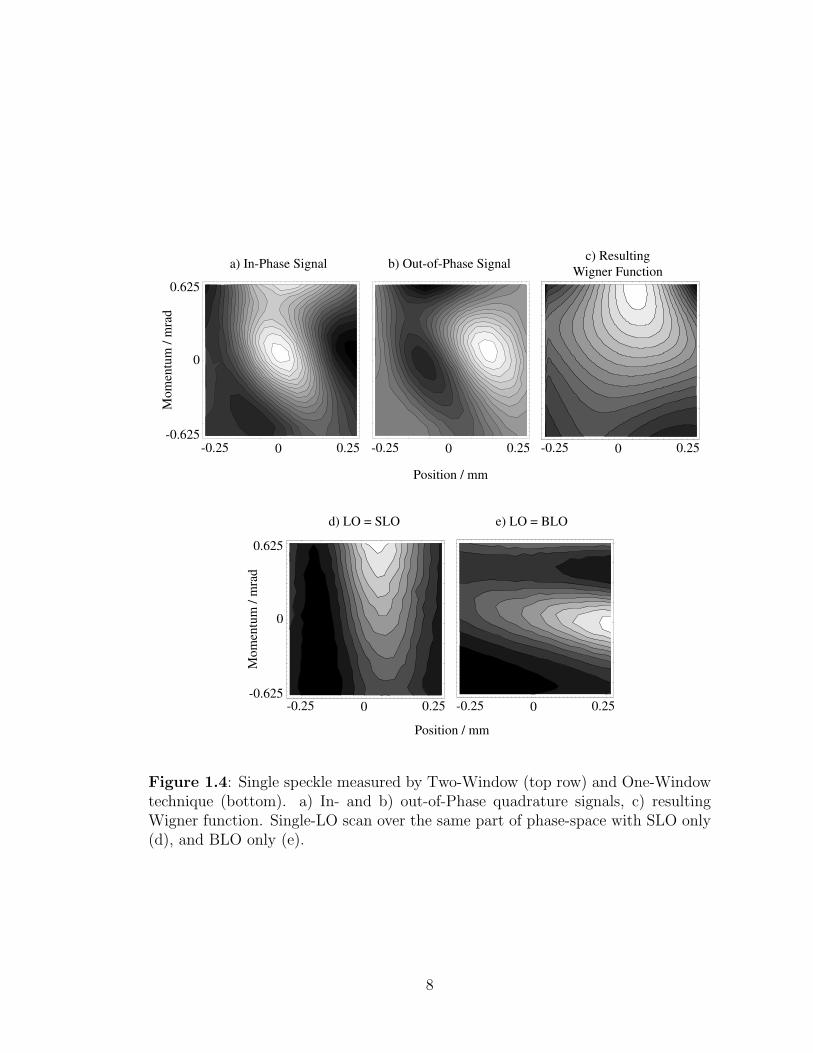
1.4 Single speckle measured by Two- and One-Window technique . . . 8

2.1 Setup for Optical Coherence Tomography (OCT) . . . . . . . . . . 22

2.2 Optical Coherence Tomography (OCT) compared to Optical Coher-ence Microscopy (OCM) . . . . . . . . . . . . . . . . . . . . . . . . 24

3.1 Wigner functions and corresponding ray diagrams . . . . . . . . . . 31

4.1 Experimental setup for Single-Window technique and HeNe . . . . . 41

4.2 Dependence of measured momentum p on translation dp . . . . . . 43

4.3 Principle of balanced detection scheme . . . . . . . . . . . . . . . . 44

4.4 Block diagram for automated data acquisition . . . . . . . . . . . . 47

4.5 Experimental setup for Single-Window technique and SLD . . . . . 48

4.6 Subscript notation for Γ . . . . . . . . . . . . . . . . . . . . . . . . 50

5.1 Experimental setup for Two-Window technique and SLD . . . . . . 60

5.2 Dual-LO measures Signal field . . . . . . . . . . . . . . . . . . . . . 70

5.3 Simulation of typical SB for flat Gaussian Signal field . . . . . . . . 74

5.4 Block diagram of phase-locked loop (PLL) . . . . . . . . . . . . . . 80

xvii

5.5 4f system . . . . . . . . . . . . . . . . . . . . . . . . . . . . . . . . 83

5.6 Complete experimental setup for Two-Window technique . . . . . . 85

6.1 z-scan of the SLD light . . . . . . . . . . . . . . . . . . . . . . . . . 90

6.2 Collimation of SLD light . . . . . . . . . . . . . . . . . . . . . . . . 92

7.1 Practical way to measure xm and pm . . . . . . . . . . . . . . . . . 113

7.2 Quadrature signals for divergent Gaussian beam . . . . . . . . . . . 124

7.3 Projections of quadrature signals for divergent Gaussian beam . . . 125

8.1 Quadrature signals for collimated Gaussian beam . . . . . . . . . . 129

8.2 x- and p−plots for in-phase quadrature signal . . . . . . . . . . . . 130

8.3 Measured Wigner function of flat Signal beam . . . . . . . . . . . . 132

8.4 Points of intersection of the out-of-phase part peaks with the dx = 0and px = 0 line. . . . . . . . . . . . . . . . . . . . . . . . . . . . . . 135

8.5 Measured momentum-integrated Wigner function of a divergent Gaus-sian beam . . . . . . . . . . . . . . . . . . . . . . . . . . . . . . . . 136

9.1 Data- Dual-LO z-scan of a Gaussian beam #1 . . . . . . . . . . . . 140

9.2 Data- Dual-LO z-scan of a Gaussian beam #2 . . . . . . . . . . . . 141

9.3 Numerical simulation of quadrature signals for z-scan of Gaussian beam144

9.4 Measured spectrum and ripple of SLD . . . . . . . . . . . . . . . . 148

9.5 Correlation function . . . . . . . . . . . . . . . . . . . . . . . . . . 149

10.1 Various scattering regimes . . . . . . . . . . . . . . . . . . . . . . . 155

10.2 Mie-plots . . . . . . . . . . . . . . . . . . . . . . . . . . . . . . . . 159

11.1 Principle of Anderson localization . . . . . . . . . . . . . . . . . . . 165

xviii

11.2 Principle of EBS . . . . . . . . . . . . . . . . . . . . . . . . . . . . 166

11.3 Notation for counter-propagating rays . . . . . . . . . . . . . . . . . 167

11.4 Probability density P . . . . . . . . . . . . . . . . . . . . . . . . . . 172

12.1 Setup close to sample container for EBS measurements . . . . . . . 193

12.2 Two-Window measurement of EBS from flat incident beam, 150 mi-cron path-delay . . . . . . . . . . . . . . . . . . . . . . . . . . . . . 198

12.3 Two-Window measurement of EBS from flat incident beam, 185 mi-cron path-delay . . . . . . . . . . . . . . . . . . . . . . . . . . . . . 199

12.4 Setup modification for EBS experiment with curved incident wavefront200

12.5 Quadrature signals and Wigner functions for divergent incident beamand convergent EBS cone. . . . . . . . . . . . . . . . . . . . . . . . 202

12.6 Quadrature signals for convergent incident beam and divergent EBScone . . . . . . . . . . . . . . . . . . . . . . . . . . . . . . . . . . . 205

12.7 Converging EBS cone detected with Two-Window technique andSingle-Window-technique . . . . . . . . . . . . . . . . . . . . . . . . 207

12.8 Position-integrated momentum distribution of EBS cone . . . . . . 208

12.9 Theory: Momentum distribution for various path-delays . . . . . . 210

13.1 Experimental setup for transmission measurements . . . . . . . . . 214

13.2 Transmission phase-space profiles, One-Window technique, variouspath delays . . . . . . . . . . . . . . . . . . . . . . . . . . . . . . . 215

13.3 Transmission phase-space profiles, One-Window technique, variousconcentration of scatterers . . . . . . . . . . . . . . . . . . . . . . . 216

13.4 Comparison of phase-space profiles with two models . . . . . . . . . 217

13.5 Two-column pattern . . . . . . . . . . . . . . . . . . . . . . . . . . 219

13.6 Momentum-integrated two-column pattern . . . . . . . . . . . . . . 220

13.7 Transmission phase-space profiles, Two-Window technique . . . . . 221

xix

13.8 Closeup transmission peak, Two-Window technique . . . . . . . . . 222

13.9 Incident beam blocked by wire, Two-Window technique . . . . . . . 223

13.10Closeup transmission peak with incident beam blocked by wire, Two-Window technique . . . . . . . . . . . . . . . . . . . . . . . . . . . 224

A.1 Circuit diagram of the temperature control . . . . . . . . . . . . . . 234

A.2 Circuit diagram of the off-board switch . . . . . . . . . . . . . . . . 234

A.3 Circuit diagram of the SLD power supply . . . . . . . . . . . . . . . 235

A.4 Circuit diagram of the phase-locked loop . . . . . . . . . . . . . . . 236

C.1 Single-scattering model . . . . . . . . . . . . . . . . . . . . . . . . . 256

C.2 Double-scattering model . . . . . . . . . . . . . . . . . . . . . . . . 259

D.1 Speckle field . . . . . . . . . . . . . . . . . . . . . . . . . . . . . . . 269

D.2 Speckle scanned by one LO . . . . . . . . . . . . . . . . . . . . . . 270

D.3 Wigner function of single speckle . . . . . . . . . . . . . . . . . . . 270

xx

Chapter 1

Introduction

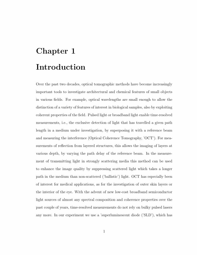
Over the past two decades, optical tomographic methods have become increasingly

important tools to investigate architectural and chemical features of small objects

in various fields. For example, optical wavelengths are small enough to allow the

distinction of a variety of features of interest in biological samples, also by exploiting

coherent properties of the field. Pulsed light or broadband light enable time-resolved

measurements, i.e., the exclusive detection of light that has travelled a given path

length in a medium under investigation, by superposing it with a reference beam

and measuring the interference (Optical Coherence Tomography, ’OCT’). For mea-

surements of reflection from layered structures, this allows the imaging of layers at

various depth, by varying the path delay of the reference beam. In the measure-

ment of transmitting light in strongly scattering media this method can be used

to enhance the image quality by suppressing scattered light which takes a longer

path in the medium than non-scattered (’ballistic’) light. OCT has especially been

of interest for medical applications, as for the investigation of outer skin layers or

the interior of the eye. With the advent of new low-cost broadband semiconductor

light sources of almost any spectral composition and coherence properties over the

past couple of years, time-resolved measurements do not rely on bulky pulsed lasers

any more. In our experiment we use a ’superluminescent diode (’SLD’), which has

1

a transverse coherence close to a laser diode but longitudinal coherence length of

just 25 microns. In Chapter 2 I will give an overview over the most common optical

tomographic methods.

In this dissertation I present a novel Two-Window Heterodyne method which

allows the direct measurement of the Wigner function of a light field [1]. Wigner

functions are a convenient way to fully characterize light fields up to their first-order-

coherence properties: A Wigner function simultaneously describes the transverse

position and momentum of a light field while preserving all phase and amplitude

information of the field. Wigner functions obey rigorous transport equations and

are a convenient way to describe the propagation of fields, through turbid, multiple

scattering media, for example.

Our Two-Window technique allows the phase-sensitive measurement of light

fields, unlike intensity measurements, as well as the immediate distinction between

coherent and incoherent contributions to the field, unlike the Single-Window tech-

nique employed previously [2–5].

We use the Two-Window technique to classify the beams generated by our SLD,

i.e., its transverse phase front as well as its first-order coherence properties both

transversely and longitudinally. The main part of this thesis deals with the mea-

surements of Wigner functions backscattered and transmitted through turbid me-

dia. Our method allows the immediate distinction between coherent and incoherent

light exiting the medium. It allows us to observe Enhanced Backscattering (”EBS”),

which causes the intensity of backscattered light to be twice as big opposite of the

direction of incidence than in other directions, thanks to constructive interference

of pairs of wavelets oppositely travelling along the same sequence of scatterers. For

the first time we are able to observe the change of sign of the radius of curvature for

2

a curved wavefront experiencing EBS: A divergent beam incident on the medium

generates a converging wavefront exiting the sample, and the other way around.

We also observe conservation of coherence for scattered light in transmission,

and look inside the speckle. The presented study will hopefully open new avenues

to examine and classify light fields in various fields, in particular in biomedical

imaging. In the following, I will briefly outline the inner workings of the Two-

Window technique.

1.1 Wigner functions and their measurement

Wigner functions describe the position and momentum distribution of a light field

in a plane perpendicular to its direction of propagation and contains all phase- and

amplitude information about it. It is Fourier-transform related to the correlation

function Γ(x, x′) = 〈E∗(x)E(x′)〉 of the field:

W (x, p) =

∫dε

2πexp(iεp)〈E∗(x +

ε

2)E(x− ε

2)〉 (1.1)

For Gaussian beams, the Wigner function bears many similarities to the geometrical

description of rays; for all other fields though it contains negative interference terms.

A detailed treatment of Wigner functions is given in Chapter 3.

In this thesis, we present a novel Two-Window heterodyne detection scheme

which allows the mapping of the true Wigner function in a given direction within

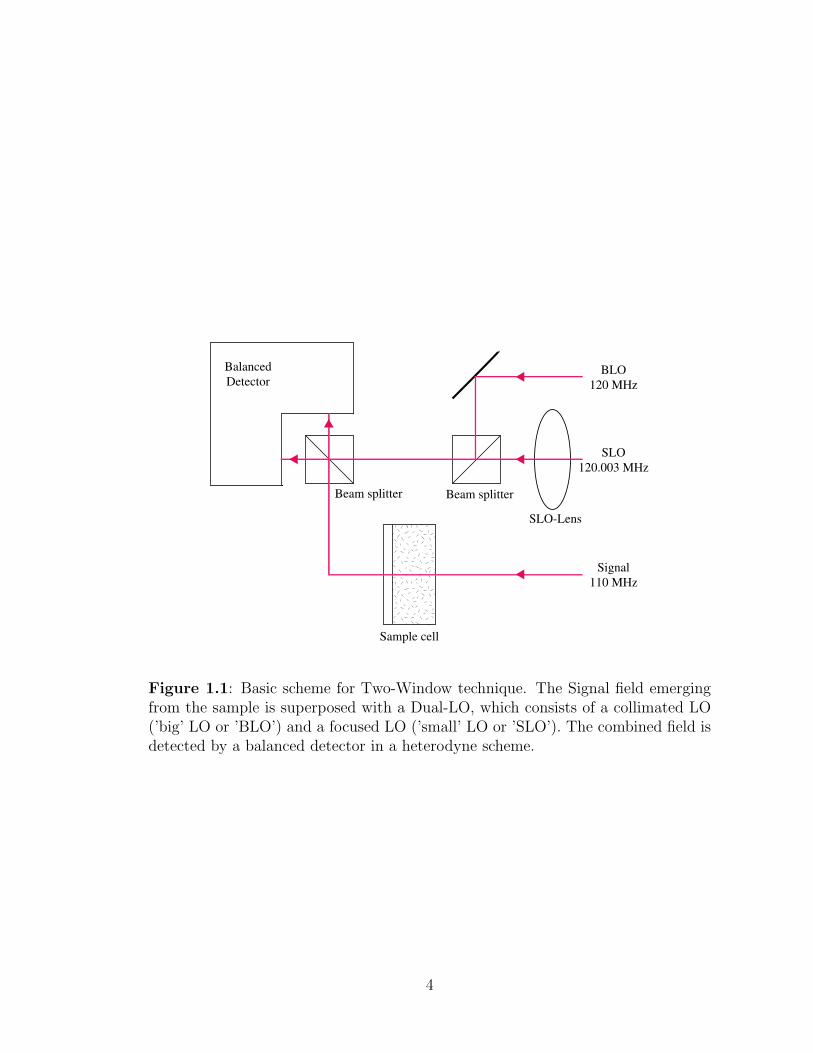
a transverse plane [1]. Figure 1.1 demonstrates how it works: A signal beam is

frequency shifted by means of an acousto-optical modulator by 110 MHz and inci-

dent on to a sample. The emerging field is superposed with a combination of two

local oscillator beams (’Dual-LO’), each LO shifted by 120 MHz and 120.003 MHz

3

SLO 120.003 MHz

BLO 120 MHz

Signal 110 MHz

SLO-Lens

Beam splitterBeam splitter

Sample cell

Balanced Detector

Figure 1.1: Basic scheme for Two-Window technique. The Signal field emergingfrom the sample is superposed with a Dual-LO, which consists of a collimated LO(’big’ LO or ’BLO’) and a focused LO (’small’ LO or ’SLO’). The combined field isdetected by a balanced detector in a heterodyne scheme.

4

respectively. This Dual-LO consists of a focused beam (”SLO”) and collimated

(”BLO”) beam; the SLO determining the spatial resolution, the BLO the angular

distribution. The two beat notes at 10 and 10.003 MHz are detected while moving

the Dual-LO relative to the Signal field in a grid-like fashion in position and mo-

mentum. The relative phase between the two beat notes is measured by a Lock-In

amplifier, whose quadrature signals then contain all the information necessary to

calculate the field’s Wigner function. Those quadrature signals are recorded during

the scanning process and the Wigner function is retrieved afterwards by performing

a simple transformation.

Like the One-Window technique, the Two-Window technique has a high dynamic

range of 130 dB [5], with the lowest detectable power level of about 10−16 W (300

photons/s).

The resolution for position and momentum in this technique can be adjusted

individually, unlike in the Single-LO technique, where a single LO causes a trade-

off between position x- and momentum p-resolution, due to the inverse relationship

between spread of x and p of the LO. Therefore, the Two-Window technique has

a much better phase-space resolution than the Single-LO technique; it allows the

measurement of true as opposed to smoothed Wigner functions. Figure 1.2 shows

the sizes of a single-LO (a) and a Dual-LO (b) in phase-space, which determine the

resolution in each method.

The high resolution and phase sensitivity allows new measurements of interesting

coherent phenomena in turbid media, like the Enhanced Backscattering effect. This

effect describes the enhancement of backscattering opposite to the direction of inci-

dence of a field, due to the coherent addition of time-reversed counter-propagating

wavelets scattered by the same sequence of scatterers in the turbid medium. Using

5

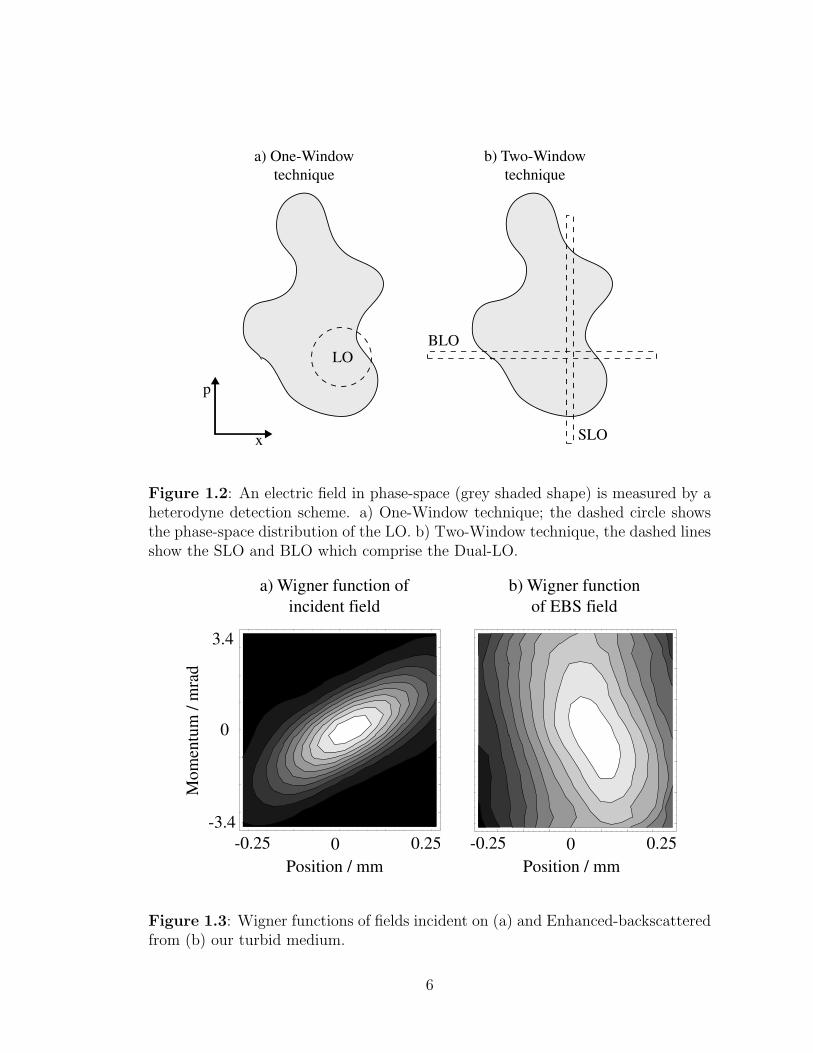
a) One-Window technique

b) Two-Window technique

LOBLO

SLOx

p

Figure 1.2: An electric field in phase-space (grey shaded shape) is measured by aheterodyne detection scheme. a) One-Window technique; the dashed circle showsthe phase-space distribution of the LO. b) Two-Window technique, the dashed linesshow the SLO and BLO which comprise the Dual-LO.

3.4

-3.4

0

-0.25 0.250 -0.25 0.250Position / mm Position / mm

Mom

entu

m /

mra

d

a) Wigner function of incident field

b) Wigner function of EBS field

Figure 1.3: Wigner functions of fields incident on (a) and Enhanced-backscatteredfrom (b) our turbid medium.

6

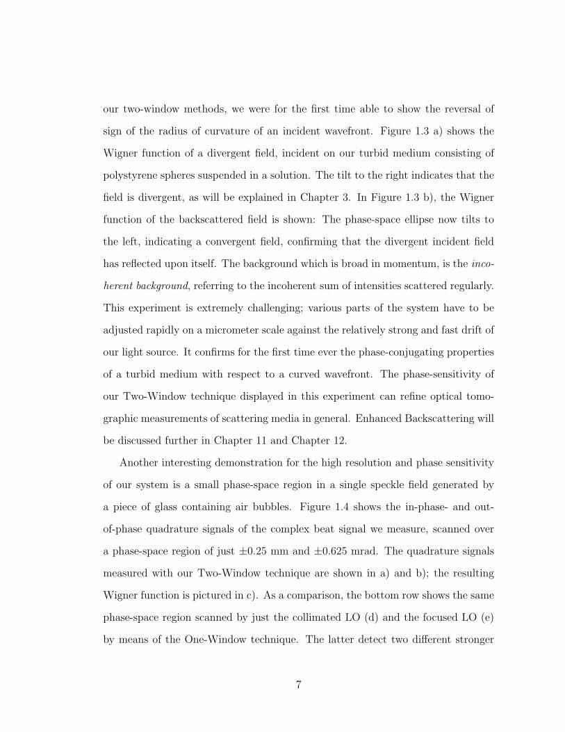
our two-window methods, we were for the first time able to show the reversal of

sign of the radius of curvature of an incident wavefront. Figure 1.3 a) shows the

Wigner function of a divergent field, incident on our turbid medium consisting of

polystyrene spheres suspended in a solution. The tilt to the right indicates that the

field is divergent, as will be explained in Chapter 3. In Figure 1.3 b), the Wigner

function of the backscattered field is shown: The phase-space ellipse now tilts to

the left, indicating a convergent field, confirming that the divergent incident field

has reflected upon itself. The background which is broad in momentum, is the inco-

herent background, referring to the incoherent sum of intensities scattered regularly.

This experiment is extremely challenging; various parts of the system have to be

adjusted rapidly on a micrometer scale against the relatively strong and fast drift of

our light source. It confirms for the first time ever the phase-conjugating properties

of a turbid medium with respect to a curved wavefront. The phase-sensitivity of

our Two-Window technique displayed in this experiment can refine optical tomo-

graphic measurements of scattering media in general. Enhanced Backscattering will

be discussed further in Chapter 11 and Chapter 12.

Another interesting demonstration for the high resolution and phase sensitivity

of our system is a small phase-space region in a single speckle field generated by

a piece of glass containing air bubbles. Figure 1.4 shows the in-phase- and out-

of-phase quadrature signals of the complex beat signal we measure, scanned over

a phase-space region of just ±0.25 mm and ±0.625 mrad. The quadrature signals

measured with our Two-Window technique are shown in a) and b); the resulting

Wigner function is pictured in c). As a comparison, the bottom row shows the same

phase-space region scanned by just the collimated LO (d) and the focused LO (e)

by means of the One-Window technique. The latter detect two different stronger

7

-0.25 0.250 -0.25 0.250 -0.25 0.250

-0.25 0.250 -0.25 0.250

0.625

-0.625

0

0.625

-0.625

0

Position / mm

Mom

entu

m /

mra

d

Mom

entu

m /

mra

d

d) LO = SLO e) LO = BLO

a) In-Phase Signal b) Out-of-Phase Signal c) Resulting Wigner Function

Position / mm

Figure 1.4: Single speckle measured by Two-Window (top row) and One-Windowtechnique (bottom). a) In- and b) out-of-Phase quadrature signals, c) resultingWigner function. Single-LO scan over the same part of phase-space with SLO only(d), and BLO only (e).

8

speckles outside the scanned region (as larger scans reveal) and yield insufficient

information about the field inside the scanned region. The Two-Window technique,

on the other hand, provides immediate phase-information of the field in the region

and allows the retrieval of the true Wigner function, as seen in (c).

The low coherence length of 24.9 µm of our light source enables the selection

of light having travelled a given path length. This is done by exploiting the fact

that two fields from the same light source only interfere when the path travelled is

equal within the longitudinal resolution ∆lB =21 µm. For scattering experiments

in transmission, this allows the suppression of the ballistic (i.e., non-scattered)

component through selection of a non-zero path-delay, which for dilute media is

much stronger than the scattered components. Light backscattered and transmitted

at various path delays also provide information about the properties of scatterers

and medium. For example, in Enhanced Backscattering, the narrowing of the EBS

cone with increasing path delay determines the scattering parameters such as the

mean free path l and the transport mean free path l∗. Additional features, such

as the momentum side-peaks of the EBS cone we observe, potentially hint towards

aberrations from the diffusion regime. In transmission, time-resolution helps resolve

the question about the contribution of various orders of scattering to the scattered

field (see Chapter 13).

In summary, our Two-Window technique presents a new way to fully characterize

a light field by measuring its Wigner function. A Wigner function contains all

phase- and amplitude information contained in the field and obeys strict propagation

laws. Our technique allows for the immediate distinction between coherent and

incoherent parts of a light field, unlike the previously employed Single-Window

technique. We apply the Two-Window technique to the determination of beam

9

parameters such as beam-size, curvature, and transverse and longitudinal coherence;

the characterization of speckle, and to the study of propagation of light fields in

turbid media.

1.2 Thesis organization

In Chapter 2 I will give an overview over the most important optical tomography

methods. The two methods for path-resolved tomography, in the time- and in the

frequency domain, are presented first. Thereafter, resolution enhancing techniques

and those gaining information on chemical composition are briefly described. The

chapter concludes with a section on Optical Coherence Tomography (OCT) and

-Microscopy (OCM), which are related to our experiment.

In Chapter 3 we introduce the Wigner function. It basic properties, including

both coherent and incoherent light, are presented, and its behavior during propaga-

tion through linear optical systems, in particular free space and lenses, are discussed.

The One-Window technique, which is the basis for the Two-Window technique,

will be presented in Chapter 4. In addition to the experimental setup and its

components we will discuss the measured mean square beat signal and its relation

to the Wigner function as well as its shortcomings that triggered the development of

the Two-Window technique. In Chapter 5 we present the Two-Window technique.

Again, the experimental setup is described , the complex beat signal measured for

ideal and non-ideal LOs and the retrieval of the true Wigner function are discussed.

This chapter concludes with a description of essential parts of the Two-Window

technique like the phase-locked loop and an overview of the complete system.

Chapter 6 presents the optical properties superluminescent diode (SLD) and

its control gadgets used in our experiment: its power-supply and temperature-

10

stabilization. The generation of a collimated Gaussian beam from the SLD output

field is described, as well as countermeasures against drift and beam instabilities.

Chapter 7 and Chapter 8 present the theoretical footing and the experimen-

tal results of the characterization of the transverse beam profile of the SLD using

our Two-Window technique. Chapter 9 presents the corresponding results for the

longitudinal beam characteristics of the SLD.

The second part of this thesis deals with scattering in turbid media. Chapter 10

describes the basics of scattering theory. The most important single-scattering

models are discussed, which describe the amplitude of an electromagnetic wave

scattering from a single particle for a range of special cases. In the second part of

this chapter the most important models for the propagation of light in turbid media

of various concentrations are presented.

In Chapter 11 and Chapter 12, theory and experimental results for our exper-

iment on Enhanced Backscattering are presented. Chapter 11 discusses the basic

principles of EBS to the complex beat signal measured for low-coherence light.

Chapter 12 shows our experimental results for flat and curved incident beams.

Finally, Chapter 13 examines scattering in dilute media. The contributions of

various orders of scattering as well as the preservation of coherence in scattered light

are investigated. Chapter 14 concludes this thesis with a summary and discusses

future directions.

11

Chapter 2

Optical Tomography Methods

2.1 Introduction

With the advent of technologies enabling the engineering of semiconductor light

sources covering a spectrum from the far infrared to the far ultraviolet and almost

arbitrary coherence properties and beam profiles, optical tomography of biological

and non-biological materials has experienced a dramatic boost. This is especially

true for time-resolved measurements which formerly depended on large and ex-

pensive femto-second lasers but can now be performed by small and inexpensive

broadband superluminescent diodes (SLDs).

A field especially interesting for optical tomography is the medical field, where

light backscattered from or generated in a sample provides insight about structural

and chemical composition of biological tissue. A general feature of these samples

is that the light experiences scattering and absorption between the surface and the

tissue layer or object of interest. While some techniques contain ways to elimi-

nate scattered or out-of-focus light, others collect that light for additional gain of

information.

For example, a relatively common procedure these days is the examination of

light backscattered from skin tissue to detect architectural abnormalities which can

12

be an indicator for cancer, in particular melanoma [6, 7]. Various methods which

measure the way light diffuses through breast tissue enable the detection of tumors

of less than 1 cm diameter before metastasis occurs and treatment becomes more

difficult [8, 9].

Optical methods also provide a safe way to image cerebral oxygenation, blood

volume by exploiting the characteristic absorption by hemoglobin, which acts as

a natural contrast agent. But also artificial contrast agents like indocyanine have

been administered for example to monitor blood flow optically [8].

Most optical techniques which examine the chemical composition of a sample

make use of light generated in the sample by fluorescence, two- or multiple-photon

processes or Raman scattering. The intensity, frequency composition or temporal

profile of the response can be an indicator for the type and concentration of a

chemical in question.

There are many approaches to push the spatial resolution for an optical method

beyond the limit dictated by the wavelength of the used light. Two of the most

important techniques are Near-field scanning optical microscopy (NSOM) and de-

convolution which are presented in Section 2.5.1 and Section 2.5.2.

In the following sections I will give a brief overview over the most prominent

optical tomography methods which are being developed today.

2.2 Time domain methods

Time domain methods use ultrashort light pulses or broadband light with a sim-

ilar coherence time to obtain time-resolution, which in turn provides path-length

resolution in the medium once the local speed of light is known. In the simplest

case, femtosecond pulses of laser light are incident on a sample and the intensity of

13

the emerging light is measured by a streak camera [10–12]. 1 Ultra-fast Kerr gates

provide another way of time-gating [14, 15]. Time-gating using broadband sources

exploits the fact that two beams generated by the same light source only interfere

if the difference in the paths they have travelled is within the coherence length of

the light. By shining one beam onto the sample and superposing the emerging light

with a second beam, only the parts of the field which match the path delay of the

second beam contribute to interference, all other parts average out due to the ran-

dom phase of broad band light. The interference signal can be measured by homo-

or heterodyne detection. We postpone a more detailed explanation to Section 2.8,

where we introduce Optical Coherence Tomography (OCT) which is a precursor to

our experiment.

By varying the time delay of the trigger for the streak camera in case of the

femtosecond laser setup or the path delay in case of a broadband source, light that

has travelled a given additional path in the medium can be exclusively detected [10,

11]. In transmission, ballistic, i.e. non-scattered light can be selected, which arrives

first at the opposite surface of the sample (path delay equals zero) [12]. This way

scattered light can be suppressed, which enhances the visibility of objects hidden in

the sample. The intensity of the ballistic light decreases exponentially with distance;

the exponent is proportional to the sum of the absorption and scattering coefficients.

For near-infrared light incident on most skin tissue, the ballistic component drops

below the detection level after a few millimeters.

A deeper penetration into turbid media is possible by analyzing the scattered

light component. In the transmission case, this component reaches the sample

surface after the ballistic component, since it travels a longer path. Time gating

1A streak camera measures ultrafast light phenomena (resolution about 0.2 ps or 60 µm lightadvancement) and delivers intensity vs. time vs. position (or wavelength) information [13].

14

allows the selection of scattered light of a given path delay here as well; its amplitude

or intensity as a function of path delay contain information about the concentration

and properties of the scatterers in the sample. A more detailed treatment of light

transmitted through turbid media is given in Chapter 13.

These time domain methods can also be used for fluorescence imaging methods

[16], as described in Section 2.4.

2.3 Frequency domain methods

Frequency domain methods examine how light modulated at radio frequency prop-

agates in a medium by measuring phase changes of the sideband frequencies with

respect to the carrier frequency. A way to study how light diffuses in highly scat-

tering media is to amplitude modulate the incident light and measure the resulting

photon density waves in the medium [17]. These density waves have been shown to

display refraction at boundaries [18], scattering and wavelength transduction [19]

(look up transduction) as well as interference patterns [20]. This method has been

used to locate breast tumors smaller than the critical size of 1 cm [21–23].

The aforementioned measurement of density waves is part of the wider field

of modulation spectroscopy, which employs an amplitude- or frequency-modulated

incident light field or combination thereof. For example, when a purely amplitude-

modulated light field is passed through a medium that displays sufficiently strong

frequency dependent propagation characteristics, the emerging field can be partially

frequency-modulated [24]. This happens if the sidebands which are in phase for

the incident light travel a different (optical) distance, leading to phase difference

between them for the emerging field. From the degree of frequency modulation,

information on narrow atomic states in the sample can be gained (i.e., trapping

15

defects in semiconductors or absorption states in gas).

2.4 Optical techniques using fluorescence

2.4.1 Multiphoton Fluorescence Microscopy

In Multiphoton Spectroscopy, femtosecond lasers serve as a light source for multi-

photon excitation of organic fluorophores 2 [25] embedded in samples. Fluorophores

can be designed so they are selectively absorbed in the specific area of a tissue under

investigation [26]. The incident long-wavelength light (e.g., infrared) is projected

onto the sample by a microscope objective. At high photon densities as in the focal

spot, two or more photons can be simultaneously absorbed by mediation of a virtual

state. The energies of those photons add up, leaving the fluorophore in an excited

state. From this state, the fluorophore drops back into its original state by emit-

ting a photon of higher energy than the exciting photons, generally in the visible

spectrum. The resulting intensity of the fluorescence is measured as a function of

the location of the focal spot.

As mentioned before, the required high photon density is only given in the fo-

cal point of the microscope objective (a micron thick at high numerical aperture),

thereby diminishing background fluorescence and out-of-focus flare that typically

limits the sensitivity in confocal microscopy. For the same reason, photodamage

is minimized which is an important limiting factor in imaging living cells, thereby

enabling the examination of thick living tissue specimen. By translating the fo-

cal point in all three dimensions and recording the intensity of the fluorescence,

three-dimensional images with micron-resolution can be captured [25]. Two-photon

2an excited fluorescent molecule releases (part of) its energy by emitting a photon.

16

microscopy has developed into a standard technique of biomedical imaging.

2.4.2 Fluorescence Lifetime Imaging (FLIM)

In Fluorescence Lifetime Imaging Microscopy (FLIM), the temporal profile of the

fluorescence is measured rather than the absolute intensity [16,27]. This is especially

useful for greater depth, where the quantitative measurement of fluorescent intensity

becomes increasingly difficult due to absorption and scattering in the tissue [26].

The fluorescence lifetime is a function of the fluorophore environment because the

non-radiative decay rate depends on the interaction with the surrounding molecules.

The fluorescence lifetimes can be measured by time-domain- and frequency-domain-

methods. In time-domain methods, pulsed laser-light in combination with photon

counting or other techniques described in Section 2.2 are used. In frequency-domain

methods and and for decays on the order of nano-seconds, a light field modulated

at a given radio-frequency experiences a characteristic phase-shift and attenuation

caused by a specific life-time.

FLIM is already being used for the dynamic measurement of Ca2+ and oxygen

concentrations as well as pH values with single-cell-resolution, for the characteriza-

tion of impurities in metal samples and in combustion related studies [26, 27].

2.5 Resolution-enhancing techniques

2.5.1 Near-field Scanning Optical Microscopy (NSOM)

In almost all optical spectroscopy methods, the spatial resolution is limited by the

wavelength of the light used. In Near-field Scanning Optical Microscopy (NSOM)

a tapered single-mode optical fiber probe with an aperture of less than an optical

17

wavelength is placed within a fraction of wavelength of the surface which is to be

examined [28]. The spatial resolution in this case is approximately the size of the

tip diameter; resolutions of up to 20 times better than the best conventional mi-

croscope have been obtained. By collecting the light emitted in the near-field or

by measuring the current induced by photo-excitation using a source with tunable

wavelength, the composition and electronic structure of semiconductors or bioma-

terials can be examined. Also, evanescent phenomena in waveguides and couplers

as well as temperature profiles of active devices can be studied.

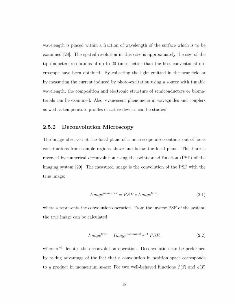
2.5.2 Deconvolution Microscopy

The image observed at the focal plane of a microscope also contains out-of-focus

contributions from sample regions above and below the focal plane. This flare is

reversed by numerical deconvolution using the pointspread function (PSF) of the

imaging system [29]. The measured image is the convolution of the PSF with the

true image:

Imagemeasured = PSF ∗ Imagetrue, (2.1)

where ∗ represents the convolution operation. From the inverse PSF of the system,

the true image can be calculated:

Imagetrue = Imagemeasured ∗−1 PSF, (2.2)

where ∗−1 denotes the deconvolution operation. Deconvolution can be performed

by taking advantage of the fact that a convolution in position space corresponds

to a product in momentum space: For two well-behaved functions f(~x) and g(~x)

18

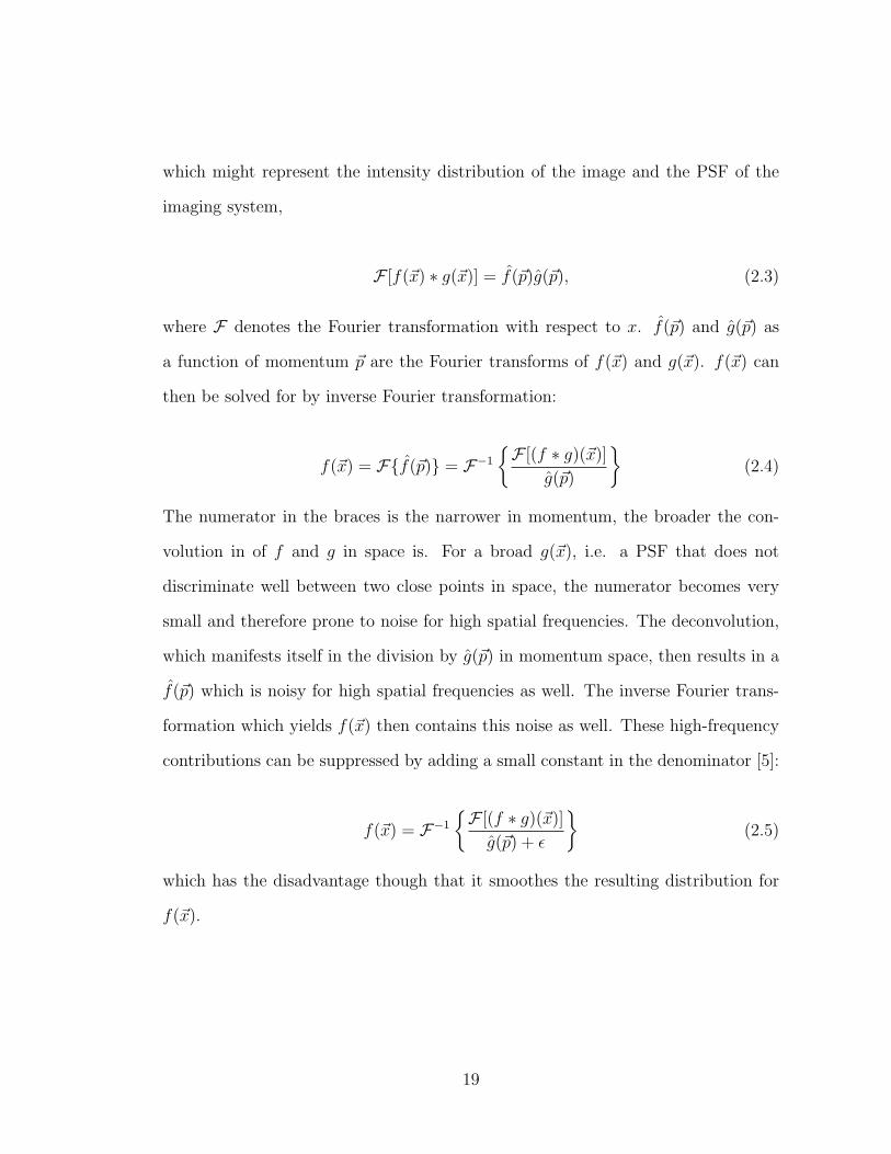
which might represent the intensity distribution of the image and the PSF of the

imaging system,

F [f(~x) ∗ g(~x)] = f(~p)g(~p), (2.3)

where F denotes the Fourier transformation with respect to x. f(~p) and g(~p) as

a function of momentum ~p are the Fourier transforms of f(~x) and g(~x). f(~x) can

then be solved for by inverse Fourier transformation:

f(~x) = Ff(~p) = F−1

F [(f ∗ g)(~x)]

g(~p)

(2.4)

The numerator in the braces is the narrower in momentum, the broader the con-

volution in of f and g in space is. For a broad g(~x), i.e. a PSF that does not

discriminate well between two close points in space, the numerator becomes very

small and therefore prone to noise for high spatial frequencies. The deconvolution,

which manifests itself in the division by g(~p) in momentum space, then results in a

f(~p) which is noisy for high spatial frequencies as well. The inverse Fourier trans-

formation which yields f(~x) then contains this noise as well. These high-frequency

contributions can be suppressed by adding a small constant in the denominator [5]:

f(~x) = F−1

F [(f ∗ g)(~x)]

g(~p) + ε

(2.5)

which has the disadvantage though that it smoothes the resulting distribution for

f(~x).

19

2.6 Optical spectroscopy for chemical analysis

2.6.1 Infrared Spectroscopy

Infrared Spectroscopy measures the absorption spectrum of infrared light of various

frequencies incident on a sample [30]. The absorption features, which are charac-

teristic for a chemical, are the results of excitations of vibrational, rotational and

bending modes of a molecule. The image contrast is solely dependent on the chem-

ical nature of the sample. A requirement for excitation by infrared radiation is

molecular asymmetry. Excitation of symmetric molecules is only possible if asym-

metric stretching or bending transitions are possible. The wavelengths in Infrared

Spectroscopy are usually in the near to mid-infrared; the wavelengths best suited

for organic compounds are in the range from 2.5 to 16 µm [31].

2.6.2 Raman spectroscopy

Raman Spectroscopy is considered a complementary technique for Infrared Spec-

troscopy. It provides information about molecular vibrations that can be used for

identification and quantification of a chemical contained in a sample. [32–34] A

rather monochromatic laser beam is directed onto the sample and the scattered

light detected by a spectrometer. While most of the scattered light will have the

same frequency as the incident light, less than 10% is frequency shifted due to energy

transfers between the incident field and vibrational energy levels of the molecules in

the sample. The various frequency lines measured around the center frequency cor-

respond to different functional group vibrations and are characteristic for a certain

chemical. The lines with a frequency below the incident field frequency are called

Stokes lines, the ones above anti-Stokes lines.

20

2.7 Confocal Microscopy

Confocal Microscopy is a technique for improving the contrast of microscope images,

particularly in thick samples. By restricting the observed volume, the technique

keeps scatterers close to the focal plane from contributing to the detected signal.

The trade-off for this is that only one point at a time can be observed [35].

In this technique, a sample is scanned by a tightly focused laser beam while the

reflected or fluoresced light is being collected by a high numerical aperture (≈ 1.4)

objective lens [36]. The high-NA objective as well as a pinhole which is introduced

into the path of light suppress out-of-focus glare which leads to improved contrast

and sharpness. The intensity of the collected light is measured by a photomultiplier

or a photo-diode. By moving the laser beam in a regular two-dimensional raster

and repeating this procedure for various depths, a three-dimensional image of the

sample can be created. The vertical resolution is on the order of 0.5 µm and the

horizontal resolution on the order of 0.2 µm [37]. Confocal Microscopy provides a

good technique for non-invasive, optical sectioning of thick living specimen.

There exist many more optical tomography methods, such as differential interfer-

ence contrast (DIC) microscopy, Optical Staining microscopy, Hoffman Modulation

Contrast Microscopy, Polarized Light Microscopy and Phase Contrast Microscopy,

which will not be discussed in this thesis. Instead, we will conclude this chapter with

the presentation of Optical Coherence Tomography, whose principle is the basis of

our experiment.

21

DetectorLateral

beam scanning

SLD

Referencemirror M

BeamSplitter

Demodulator A/D converter Computer

R

Figure 2.1: Setup for Optical Coherence Tomography (OCT).

22

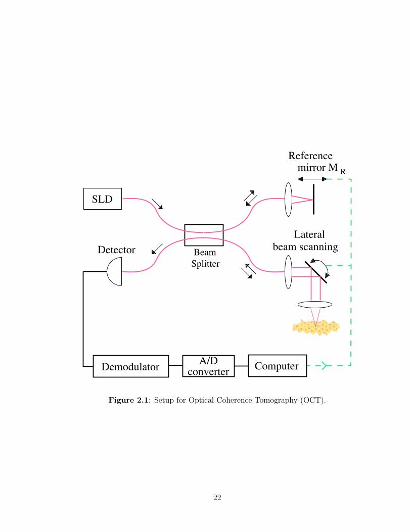
2.8 Optical Coherence Tomography (OCT)

Optical Coherence Tomography (OCT) uses a combination of the principles of low-

coherence tomography and confocal microscopy [38]. Figure 2.1 shows set setup:

two beams are generated from a broadband (or pulsed laser) source (SLD); we

will refer to them as Signal- and Local Oscillator- beam. The Signal beam is in-

cident on the sample; the transmitted or scattered light is then superposed with

the Local Oscillator beam. Due to the broad spectrum of the light, its longitudi-

nal coherence length is small; typically on the order of tens of micrometers. The

light coming from the sample and the Local Oscillator beam only interfere if their

path-length is matched within the coherence length of the light. By changing the

relative path-delay between the beams with the reference mirror (MR) and detect-

ing the interference signal of the beams at the same time, signal contributions from

different regions in the sample can be selected. In the shown setup, a map of tissue

reflectivity versus depth can be obtained (z-scan). By moving the laser beam in a

two-dimensional raster and taking z-scans for each point, similar to the procedure

described for Confocal Microscopy in Section 2.7, a three-dimensional image can be

obtained.

The interference between the Signal- and Local Oscillator beam is usually mea-

sured by means of heterodyne detection. In the most straightforward way, the

Doppler-shift introduced by the moving reference mirror MR during a depth-scan

is exploited: The interference signal will be centered at the Doppler frequency and

can easily be extracted by a lock-in amplifier, while the parts of the signal that do

not contribute to interference average out.

23

Axial Resolution determined by Depth of Focus

Lateral Resolution

OCT OCM

Low NA Focusing

Axial Resolution determined by Coherence Length

High NA Focusing

Water Immersion

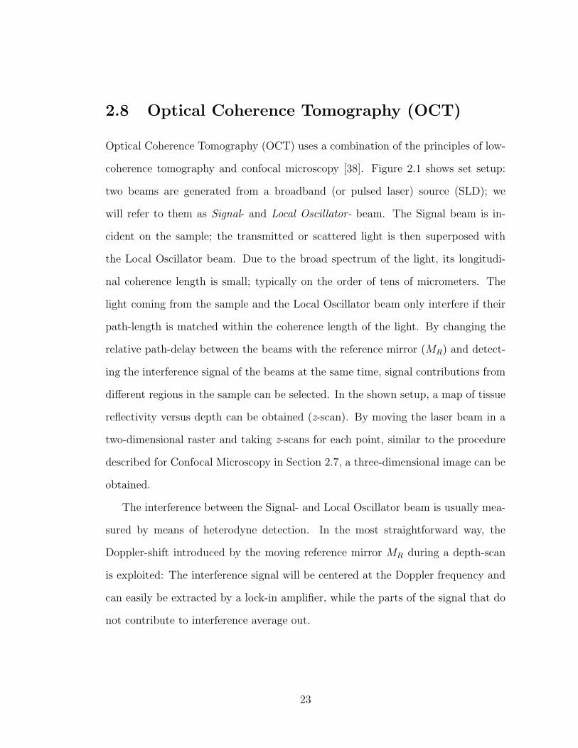
Figure 2.2: Optical Coherence Tomography (OCT, left) compared to Optical Co-herence Microscopy (OCM, right).

2.8.1 Optical Coherence Microscopy (OCM)

Optical Coherence Tomography (OCM) directly combines OCT and Confocal Mi-

croscopy [38]. While its principle is the same as that of OCT, it adds a high NA

objective in order to increase lateral and axial resolution due to the smaller focal

spot size and Rayleigh length.3 In addition the high NA objective provides en-

hanced rejection of out-of-focus or multiply scattered light. OCM can be used in

case where there are no physical constraints with respect to the distance between

the sample and the objective. Figure 2.2 demonstrates the differences between OCT

3The Rayleigh length is the distance after which a beam passing through its beamwaist growsto twice its area. It is inversely proportional to the area of the beamwaist.

24

and OCM. In the figure shown, the OCM objective is immersed in water where the

wavelength is smaller, thereby enhancing the resolution.

Since the small Rayleigh length and the strong rejection of out-of-focus light

in OCM determine the axial location of the examined plane, a longitudinal z-scan

can not be performed as easily as for OCT, using the Doppler-shift introduced by

the reference mirror, unless the focal plane of the objective is changed at the same

rate.4 This problem also arises when the reference mirror is moved stepwise and

the heterodyne signal is generated by the beat frequency of the Signal- and Local

Oscillator beams frequency-shifted by means of acousto-optic modulators.

Compared to Confocal Microscopy alone, the short coherence of the broadband

light in OCM helps rejecting light coming from above and beneath the objective

focal plane, where its point-spread function is broad.

2.8.2 Color Doppler Optical Coherence Tomography

(CDOCT)

Color Doppler Optical Coherence Tomography measures the flow of objects in a

sample by taking advantage of the additional Doppler-shift they introduce. This

way, reflections from objects moving away and towards the incident Signal beam

cause frequency components in the heterodyne signal below and above the Doppler-

frequency generated by the reference mirror. Several groups have used this tech-

niques for quantitative measurements of blood flow in tissue with micron-scale res-

olution [39, 40]. The spatial resolution in [39] is better than 45 µm in depth and

10 µm laterally, the velocity resolution on the order of 0.5 mm/s, the latter being

4This is non-trivial since the depth-dependent refractive index in the sample influences thedepth of the focal plane which has to be taken into account when adjusting the relative path delaybetween the Signal- and Local Oscillator beam.

25

easily adjustable by varying the speed of the reference mirror.

26

Chapter 3

Wigner Functions

3.1 Introduction

A central feature of this thesis is the measurement of Wigner functions to charac-

terize light fields. Wigner functions provide a convenient way to describe a light

field is by means of the Wigner function [2, 3]. Wigner functions characterize the

spatial and angular distribution of a field at the same time as well as its coherence

properties. They obey simple transport equations in first-order systems such as thin

lenses, magnifiers and free space [41] which are analogous to those in ray-optics.

A Wigner function is a real function which simultaneously describes a distribu-

tion in two conjugate variables, like time and frequency or space and momentum.

In the first case it can be compared to a musical score, which tells a musician the

frequencies of a song as a function of time. In the second case it can be considered

the local spatial frequency spectrum of a signal. The Wigner function for a Gaus-

sian beam closely resembles its ray-optical equivalent in geometrical optics [41]. For

all other types of fields Wigner functions exhibit interference terms and negative

features. Wigner functions belong to the group of so-called quasi-propabilities.

The Wigner function for a light field E(x) is

27

W (x, p) =1

2π

∫dε exp(ipε) 〈E∗(x +

ε

2)E(x− ε

2)〉

=

∫dε

2πexp(ipε) Γ(x +

ε

2, x− ε

2), (3.1)

where x is the transverse position and p the transverse momentum of the light field.

The transverse momentum p is the wave-vector k times the angle of direction θ of

a light field: p = θk. The angled brackets signifies temporal averaging for partially

coherent light fields.

For a given transverse position x, W (x, p) is the Fourier transform integral of the

mutual coherence functions Γ(x + ε2, x− ε

2) = 〈E∗(x + ε

2)E(x− ε

2)〉 centered around

x. Similarly, for a given transverse momentum p, W (x, p) is the Fourier transform

integral of the angular cross-spectral densities Γ(p+ q2, p− q

2) = 〈E∗(p+ q

2)E(p− q

2)〉

centered around p. The cross-spectral density becomes separable for coherent light,

where the averaging becomes unnecessary.

Wigner functions contain phase information about a light field (as opposed to

intensity measurements), which can easily be seen from its relationship to the mu-

tual coherence function. Therefore, they offer an attractive framework in which

to study the propagation of optical coherence through random media [42]. Previ-

ously, we have measured smoothed Wigner functions using a single beam heterodyne

method [1–4]. In that technique, the position and momentum resolution were de-

termined by the LO’s size and angular spread, which are inversely proportional to

each other and which mathematically manifests itself in an uncertainty product

associated with Fourier transform pairs.

The novel two-window technique [1] presented in this thesis allows independent

28

control over the position and momentum resolution by using a phase-coupled set of

LOs, thereby surpassing this uncertainty limit and permitting measurement of true

(vs. smoothed) Wigner functions.

3.2 Basic properties of Wigner functions

In the following, some basic properties of Wigner functions will be discussed, which

will be beneficial in understanding more complex experimental and theoretical re-

sults later on.

3.3 Wigner functions of spatially incoherent light

Spatially incoherent light, such as the broad background contribution of light experi-

encing large angle scattering in random media, can be described by the cross-spectral

density Γ(x+ 12ε, x− 1

2ε) = c(x)δ(ε) with c(x) being a non-negative function [41]. A

Fourier-transformation with respect to ε yields the corresponding Wigner function

W (x, p) = c(x) which is independent of p. This is in agreement with the property

of light to develop transverse coherence while travelling in a preferred direction: in

order to be incoherent, the field has to be direction-independent.

29

3.4 Wigner functions of a (partially) coherent

beam

Partially coherent Gaussian beams belong to the family of Gaussian Schell model

light sources and can be described by the cross-spectral density [43]

Γ(x1, x2) = 〈E∗(x1)E(x2)〉

= exp

[−x2

1 + x22

4σ2s

]exp

[−(x1 − x2)

2

2σ2g

]exp

[ik

2R(x2

1 − x22)

]. (3.2)

The corresponding Wigner function is the Fourier transformation with respect to

the difference between x1 and x2 (see Eq. (3.1)). Inserting Eq. (3.2) into Eq. (3.1)

yields:

W part.coh(x, p) =π

αexp

[− x2

2σ2s

− (kxR

+ p)2

4α

](3.3)

with α = 18σ2

s+ 1

2σ2g. The momentum spread of a light field in phase-space becomes

larger with decreasing transverse coherence length σg which is consistent with the

quintessence of Section 3.3. For finite radii of curvature, the spatial size of the field

displays a similar σg-dependence, converging towards the size we would have for a

flat wavefront. The momentum peaks at p = −kxR

.

Most laser beams can be viewed as transverse coherent, which implies σg À σs.

In that case the exponential term in the middle of Eq. (3.2) is approximately unity.

The resulting Wigner function reduces to:

W coh(x, p) =1

π2exp

[− x2

2σ2s

− 2σ2s

(kx

R+ p

)2]

(3.4)

30

Figure 3.1: Ray-diagrams and their corresponding Wigner function for a Gaussianbeam waist, and a divergent and convergent Gaussian beam.

31

Figure 3.1 shows ray-diagrams for a beam waist (a), divergent (b) and convergent

(c) beams together with their correspondent Wigner functions.

For the beam waist (R = ∞), σs is both in the denominator of the x-prefactor

and the numerator of the p-pre-factor, which confirms the inverse relationship be-

tween the size of the beam and its angular spread.

For R 6= ∞, i.e. a convergent or divergent beam, there exists a correlation be-

tween momentum and position: For a divergent beam (R positive), the momentum

distribution is centered around positive values for positive x and around negative

values for negative x. This is consistent with the physical picture of off-axis parts of

a divergent beam moving away from the center. An opposite relationship between

x and p exists for a convergent beam, seen on the right, as can easily be verified.

A Gaussian beam is the only field for which the Wigner distribution is positive

throughout phase-space. Even the combination of two Gaussian beams separated

by a distance displays negative features as part of an additional oscillating term in

momentum [5].

3.5 Integrals of Wigner functions

The integrals

I(x) =

∫dp W (x, p) (3.5)

and

I(p) =

∫dx W (x, p) (3.6)

32

are the positional and the directional intensity of the light field, whereas

P =

∫dp dx W (x, p) (3.7)

is its total power.

3.6 Propagation through linear optical systems

A linear system in optics such as a thin lens or free space can be described by two

equations which connect the position and momentum of an incident field with those

of the emerging field. For the position distribution of both fields the relationship

Ecoho (xo) =

∫dxi hxx(xo, xi)Ecoh

i (xi) (3.8)

exists, where hxx(x1, x0) is the so-called point-spread function and E0 and E1 are

the coherent incident and emerging field [41]. hxx is the response of the system in

the space domain when the input signal is a point source. Partially coherent light,

which can be described by the cross-spectral density function, displays a similar

relationship between emerging and incident field:

Γo(xo, x′o) =

∫ ∫dx dx′ hxx(xo, x)Γi(x, x′)h∗xx(x

′o, x

′). (3.9)

The Wigner function, which is Fourier-transform related to the mutual coherence

function, can be directly calculated by inserting Eq. (3.9) into Eq. (3.1), which

results in

Wo(xo, po) =

∫ ∫dxi dpi K(xo, po, xi, pi) Wi(xi, pi). (3.10)

33

K is called the ray-spread function of the system since it is the response to the

hypothetical case of a single ray with the (impossible) Wigner function Wi(x, p) =

δ(x − xi)δ(p − pi) entering the system. K can be expressed as a function of the

point-spread function hxx:

K(xo, po, xi, pi) =

∫ ∫dx′o dx′i hxx(xo +

1

2x′o, xi +

1

2x′i)h

∗xx(xo − 1

2x′o, xi − 1

2x′i)

× exp[−i(pox′o − pix

′i)]. (3.11)

This relation allows us to directly calculate the propagation of a Wigner function

through linear media. For a thin lens in the paraxial approximation the point

spread function takes the form

hxx(x1, x0) = exp

(− ik

2fx2

1

)δ(x1 − x0) (3.12)

which results in the transport equation for the Wigner function

W1(x, p) = W0(x, p +kx

f). (3.13)

A section of free space in the Fresnel approximation has the point spread

function

hxx(x1, x0) =

√k

2πizexp

[ik

2z(x1 − x0)

2

]. (3.14)

The corresponding Wigner function becomes:

W1(x, p) = W0(x− zp

k, p). (3.15)

34

Both Equations (3.13) and (3.15) are equivalent to the geometrical description of a

ray propagating through a lens or a section of free space, respectively. It should be

kept in mind though, that a Wigner function contains the full phase information of

a field.

Another interesting property of the propagation of a Wigner function in free

space is that the total time-derivative is zero, which has been verified for coherent

electromagnetic fields [5]:

dW (~x, ~p; t)

dt=

∂W (~x, ~p; t)

∂t+ ~v ·W (~x, ~p; t) = 0. (3.16)

This expression is equivalent to the Liouville’s theorem of classical mechanics, which

tells us that the density of a volume element we follow along a flow-line in phase-

space is conserved [44]. This can easily be seen by looking at Eq. (3.15): For a

given momentum p at a given distance z, the position-distribution x(p) shifts by an

offset zpk, without otherwise changing its properties. A volume element containing

an arbitrary part of the Wigner function remains constant in size, because in free

space the field does not lose energy. Therefore, the Wigner function, which is the

power density in phase-space, has to be constant as well, which proves Liouville’s

theorem in this particular case. By inspection of the corresponding expression for

propagation through a lens (Eq. (3.13)), it is clear that Liouville’s theorem should

apply for that case, too.

3.6.1 General Luneburg’s first order systems

Luneburg’s first order systems [45] display a propagation behavior of

Wo(xo, po) = Wi(Axi + Bpi, Cxi + Dpi) (3.17)

35

where the transformation parameters must obey the symplecticity condition on the

determinant

∣∣∣∣∣∣∣A B

C D

∣∣∣∣∣∣∣= 1. (3.18)

We have three free parameters here; the fourth one is determined by condition

(3.18).

As we just have seen, Liouville’s theorem holds for the first-order systems lens

and free space. It is clear that it still holds for the similar, but more general cases

where we replace the factors − zk

and kf

in Equations (3.15) and (3.13) with the

arbitrary parameters B and C from Eq. (3.17). The ABCD matrices for both

cases are then

A B

C D

lens

=

1 0

k/f 1

(3.19)

A B

C D

free space

=

1 −z/k

0 1

. (3.20)

(3.21)

B can even be negative, but in this case it does not represent the travel through

free space anymore. Let us consider an arrangement of the generalized expressions

for lens, a section of free space and another lens. It can then easily be verified

that the resulting total ABCD-transformation matrix is symplectic and represents

36

a first-order Luneburg system itself:

We consider a Wigner function W1(x, p) incident on a lens. Right after lens

L1, the Wigner function is W2(x, p) = W1(x, p + Cx). After travelling through the

generalized space, W3(x′, p′) = W2(x

′ + B′p′, p′) or

W3(x, p) = W1[x + B′(p + Cx), p + Cx]

= W1[(1 + B′C)x + B′p, Cx + p]

= W1(A′′x + B′′p, C ′′x + D′′p). (3.22)

It can easily be verified that A′′D′′−B′′C ′′ = 1 which confirms that the combination

of a lens and the distance of generalized space still represents a first-order system.

After passing lens L2, the Wigner function becomes

W4(x′′, p′′) = W3(x

′′, p′′ + C(3)x′′)

= W2[x′ + B′p′, p′ + C(3)(x′ + B′p′)]

= W1x(1 + B′C) + B′p, [C + C(3)(1 + B′C)]x + (1 + c(3)B′)p

= W1(A(4)x + B(4)p, C(4)x + D(4)p). (3.23)

A4, B4, C4 and D4 are fully determined by C,B′ and C(3) and fulfill the symplecticity

condition (3.18) for every choice of them.

The relationship of A4, B4, C4, D4 and C, B′, C(3) expressed in Eq. (3.23)

37

A(4) = 1 + B′C (3.24)

B(4) = B′ (3.25)

C(4) = C + C(3)(1 + B′C) (3.26)

D(4) = 1 + C(3)B′ (3.27)

can be solved for C,B′ and C(3):

C =A(4) − 1

B(4)(3.28)

B′ = B(4) (3.29)

C(3) =D(4) − 1

B(4)(3.30)

where B′ and C(3) can be uniquely derived from Equations (3.25) and (3.27); C

results from Eq. (3.24) and either Eq. (3.25) or Eq. (3.26) together with the

symplecticity requirement Eq. (3.18).

Since the Liouville expression holds for each one of the three-component system

just described, it will also hold for their combination. Furthermore, Eq. (3.28)

shows that an arbitrary Luneburg first-order system can be expressed as such a

three-component system. Therefore we can draw the conclusion that the Liouville

expression holds for all Luneburg first-order systems.

38

Chapter 4

The Single-Window technique

4.1 Introduction

In this section I will explain the experimental setup for the Single-Window technique

that we have been using in the past to measure smoothed Wigner functions [46].

Its basic concept is the heterodyne measurement of a signal field by means of a

single Local Oscillator (LO) beam. The Signal- and LO fields are frequency-shifted

by different amounts and superposed on a detector. The detector measures a beat

note which corresponds to the difference in frequencies of Signal- and LO fields.

Its amplitude is proportional to the overlap integral of both fields at the area of

coincidence. By stepwise changing the relative transverse position x and transverse

momentum p of the LO with respect to the Signal field and recording the beat signal,

the phase-space distribution of the Signal field can be determined. For maximum

resolution, the LO itself must be as small as possible in phase-space, that means

its diameter and angular spread must be minimal. The trade-off between small size

and angular spread can best be met by using a Gaussian beam. A Gaussian beam

of ’diameter’ a has an angular spread of about λa. Therefore, the smallest features

in the Signal field that can be measured are on the order of a in size and 1a

in

transverse momentum. The finite x- and p resolution leads to a smoothing effect of

39

the measured signal. Therefore, we refer to the Single-LO technique as a technique

for measuring ’smoothed’ Wigner functions which will be explained in the following

section Section 4.2.

In all of our experiments, we use a Superluminescent diode (SLD) as a light

source. It has a longitudinal coherence of just 24.9 µm which enables time-resolved

measurement of the signal field, as will be explained later. This short coherence

length requires additional elements in the experimental setup. A detailed treatment

will be given in Section 4.6.

The Single-LO technique used for the measurement of smoothed Wigner func-

tions serves as a basis for the Two-Window technique, which enables the mea-

surements of the true, i.e. non-smoothed Wigner function. This technique is the

centerpiece of this thesis and will be described in Chapter 5.

In the following section, I start by explaining the experimental setup for the

stationary measurement of smoothed Wigner functions, followed by a discussion of

the balanced detection system (Section 4.3), the real-time noise suppression scheme

(Section 4.4) and the automated data acquisition setup we use (Section 4.5). In Sec-

tion 4.6 the modifications for time-resolved measurements using broadband light are

discussed. The chapter is concluded in Section 4.7 with a description of the actual

measurement of time-resolved Signal fields and the retrieval of Wigner functions for

transversely coherent Signal fields.

4.2 Experimental setup with laser light source

Figure 4.1 shows the basic setup for the measurement of stationary smooth Wigner

functions. For demonstrative purposes, the setup for transmission measurements is

shown. Omitted for clarity are a 4f -system used in the signal arm as well as several

40

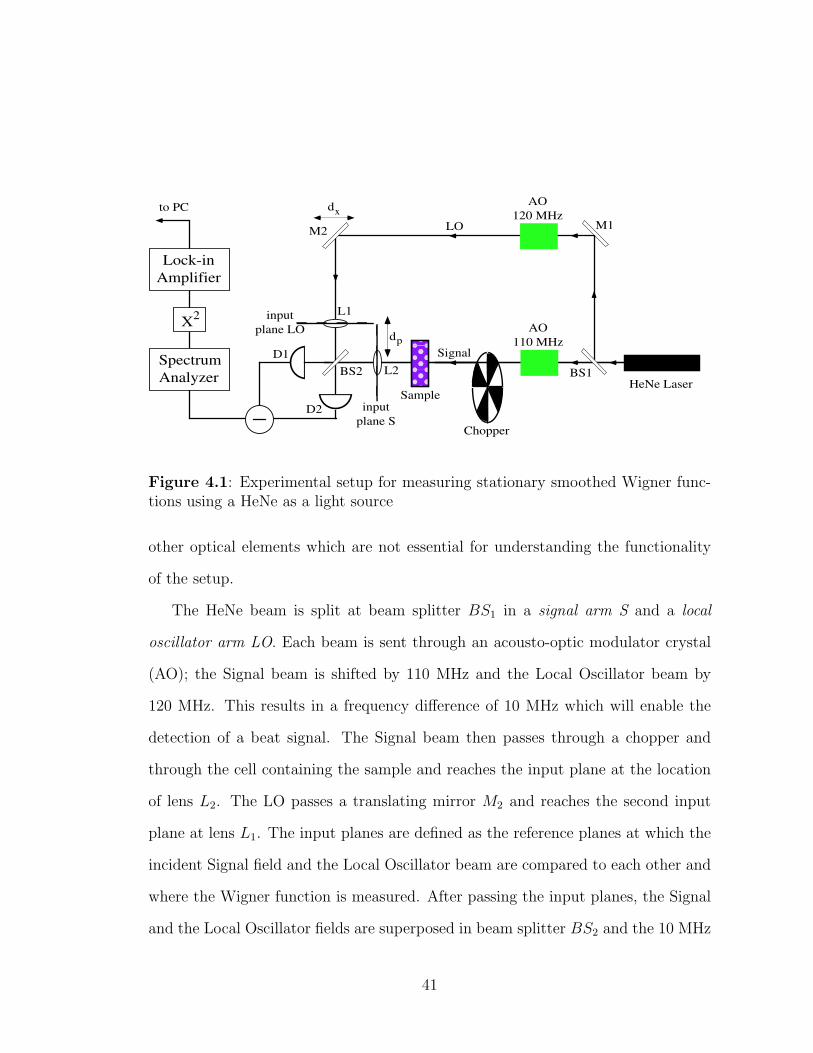
D1

M2

L2

L1

dx

dp

LO

X2

Spectrum Analyzer

Lock-in Amplifier

to PC

D2

Signal

AO 120 MHz

AO 110 MHz

Chopper

BS2

Sample

M1

BS1

input plane S

input plane LO

HeNe Laser

Figure 4.1: Experimental setup for measuring stationary smoothed Wigner func-tions using a HeNe as a light source

other optical elements which are not essential for understanding the functionality

of the setup.

The HeNe beam is split at beam splitter BS1 in a signal arm S and a local

oscillator arm LO. Each beam is sent through an acousto-optic modulator crystal

(AO); the Signal beam is shifted by 110 MHz and the Local Oscillator beam by

120 MHz. This results in a frequency difference of 10 MHz which will enable the

detection of a beat signal. The Signal beam then passes through a chopper and

through the cell containing the sample and reaches the input plane at the location

of lens L2. The LO passes a translating mirror M2 and reaches the second input

plane at lens L1. The input planes are defined as the reference planes at which the

incident Signal field and the Local Oscillator beam are compared to each other and

where the Wigner function is measured. After passing the input planes, the Signal

and the Local Oscillator fields are superposed in beam splitter BS2 and the 10 MHz

41

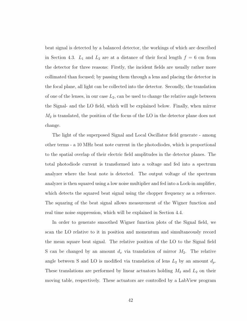
beat signal is detected by a balanced detector, the workings of which are described

in Section 4.3. L1 and L2 are at a distance of their focal length f = 6 cm from

the detector for three reasons: Firstly, the incident fields are usually rather more

collimated than focused; by passing them through a lens and placing the detector in

the focal plane, all light can be collected into the detector. Secondly, the translation

of one of the lenses, in our case L2, can be used to change the relative angle between

the Signal- and the LO field, which will be explained below. Finally, when mirror

M2 is translated, the position of the focus of the LO in the detector plane does not

change.

The light of the superposed Signal and Local Oscillator field generate - among

other terms - a 10 MHz beat note current in the photodiodes, which is proportional

to the spatial overlap of their electric field amplitudes in the detector planes. The

total photodiode current is transformed into a voltage and fed into a spectrum

analyzer where the beat note is detected. The output voltage of the spectrum

analyzer is then squared using a low noise multiplier and fed into a Lock-in amplifier,

which detects the squared beat signal using the chopper frequency as a reference.

The squaring of the beat signal allows measurement of the Wigner function and

real time noise suppression, which will be explained in Section 4.4.

In order to generate smoothed Wigner function plots of the Signal field, we

scan the LO relative to it in position and momentum and simultaneously record

the mean square beat signal. The relative position of the LO to the Signal field

S can be changed by an amount dx via translation of mirror M2. The relative

angle between S and LO is modified via translation of lens L2 by an amount dp.

These translations are performed by linear actuators holding M2 and L2 on their

moving table, respectively. These actuators are controlled by a LabView program

42

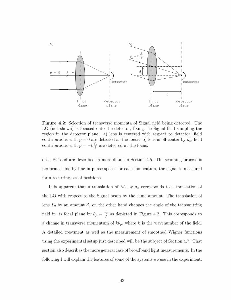
d = 0pdp

f

input plane

input plane

detector plane

detector plane

p = 0

p = d__fp_k

a) b)

Detector Detector

Figure 4.2: Selection of transverse momenta of Signal field being detected. TheLO (not shown) is focused onto the detector, fixing the Signal field sampling theregion in the detector plane. a) lens is centered with respect to detector; fieldcontributions with p = 0 are detected at the focus. b) lens is off-center by dp; field

contributions with p = −k dp

fare detected at the focus.

on a PC and are described in more detail in Section 4.5. The scanning process is

performed line by line in phase-space; for each momentum, the signal is measured

for a recurring set of positions.

It is apparent that a translation of M2 by dx corresponds to a translation of

the LO with respect to the Signal beam by the same amount. The translation of

lens L2 by an amount dp on the other hand changes the angle of the transmitting

field in its focal plane by θp = dp

fas depicted in Figure 4.2. This corresponds to

a change in transverse momentum of kθp, where k is the wavenumber of the field.

A detailed treatment as well as the measurement of smoothed Wigner functions

using the experimental setup just described will be the subject of Section 4.7. That

section also describes the more general case of broadband light measurements. In the

following I will explain the features of some of the systems we use in the experiment.

43

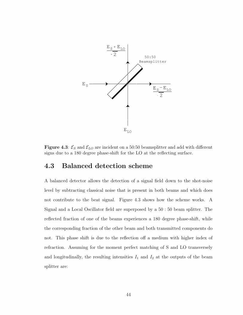
ELO

ES

50:50 Beamsplitter

ES ELO+

2

ES_ ELO2

.

.

Figure 4.3: ES and ELO are incident on a 50:50 beamsplitter and add with differentsigns due to a 180 degree phase-shift for the LO at the reflecting surface.

4.3 Balanced detection scheme

A balanced detector allows the detection of a signal field down to the shot-noise

level by subtracting classical noise that is present in both beams and which does

not contribute to the beat signal. Figure 4.3 shows how the scheme works. A

Signal and a Local Oscillator field are superposed by a 50 : 50 beam splitter. The

reflected fraction of one of the beams experiences a 180 degree phase-shift, while

the corresponding fraction of the other beam and both transmitted components do

not. This phase shift is due to the reflection off a medium with higher index of

refraction. Assuming for the moment perfect matching of S and LO transversely

and longitudinally, the resulting intensities I1 and I2 at the outputs of the beam

splitter are:

44

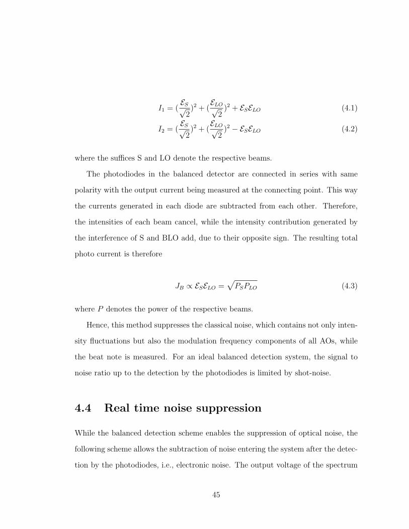
I1 = (ES√

2)2 + (

ELO√2

)2 + ESELO (4.1)

I2 = (ES√

2)2 + (

ELO√2

)2 − ESELO (4.2)

where the suffices S and LO denote the respective beams.

The photodiodes in the balanced detector are connected in series with same

polarity with the output current being measured at the connecting point. This way

the currents generated in each diode are subtracted from each other. Therefore,

the intensities of each beam cancel, while the intensity contribution generated by

the interference of S and BLO add, due to their opposite sign. The resulting total

photo current is therefore

JB ∝ ESELO =√

PSPLO (4.3)

where P denotes the power of the respective beams.

Hence, this method suppresses the classical noise, which contains not only inten-

sity fluctuations but also the modulation frequency components of all AOs, while

the beat note is measured. For an ideal balanced detection system, the signal to

noise ratio up to the detection by the photodiodes is limited by shot-noise.

4.4 Real time noise suppression

While the balanced detection scheme enables the suppression of optical noise, the

following scheme allows the subtraction of noise entering the system after the detec-

tion by the photodiodes, i.e., electronic noise. The output voltage of the spectrum

45

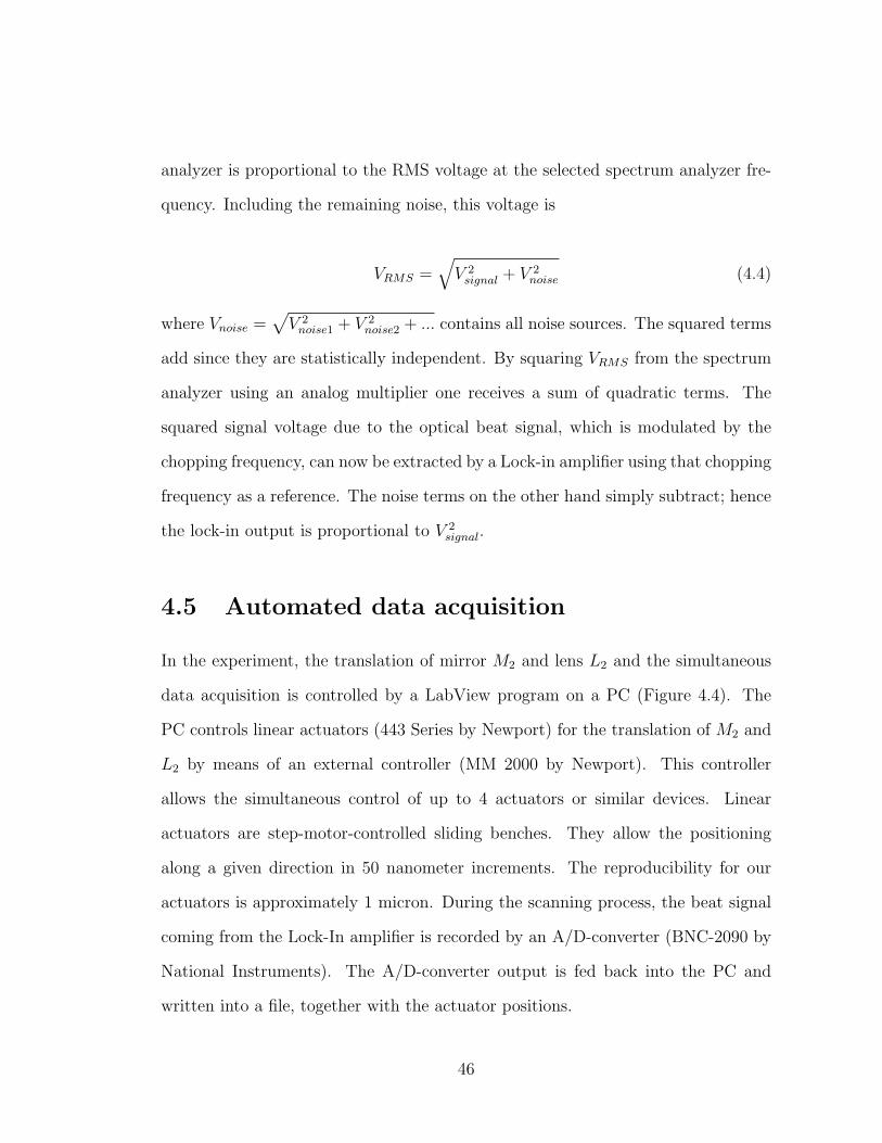
analyzer is proportional to the RMS voltage at the selected spectrum analyzer fre-

quency. Including the remaining noise, this voltage is

VRMS =√

V 2signal + V 2

noise (4.4)

where Vnoise =√

V 2noise1 + V 2

noise2 + ... contains all noise sources. The squared terms

add since they are statistically independent. By squaring VRMS from the spectrum

analyzer using an analog multiplier one receives a sum of quadratic terms. The

squared signal voltage due to the optical beat signal, which is modulated by the

chopping frequency, can now be extracted by a Lock-in amplifier using that chopping

frequency as a reference. The noise terms on the other hand simply subtract; hence

the lock-in output is proportional to V 2signal.

4.5 Automated data acquisition

In the experiment, the translation of mirror M2 and lens L2 and the simultaneous

data acquisition is controlled by a LabView program on a PC (Figure 4.4). The

PC controls linear actuators (443 Series by Newport) for the translation of M2 and

L2 by means of an external controller (MM 2000 by Newport). This controller

allows the simultaneous control of up to 4 actuators or similar devices. Linear

actuators are step-motor-controlled sliding benches. They allow the positioning

along a given direction in 50 nanometer increments. The reproducibility for our

actuators is approximately 1 micron. During the scanning process, the beat signal

coming from the Lock-In amplifier is recorded by an A/D-converter (BNC-2090 by

National Instruments). The A/D-converter output is fed back into the PC and

written into a file, together with the actuator positions.

46

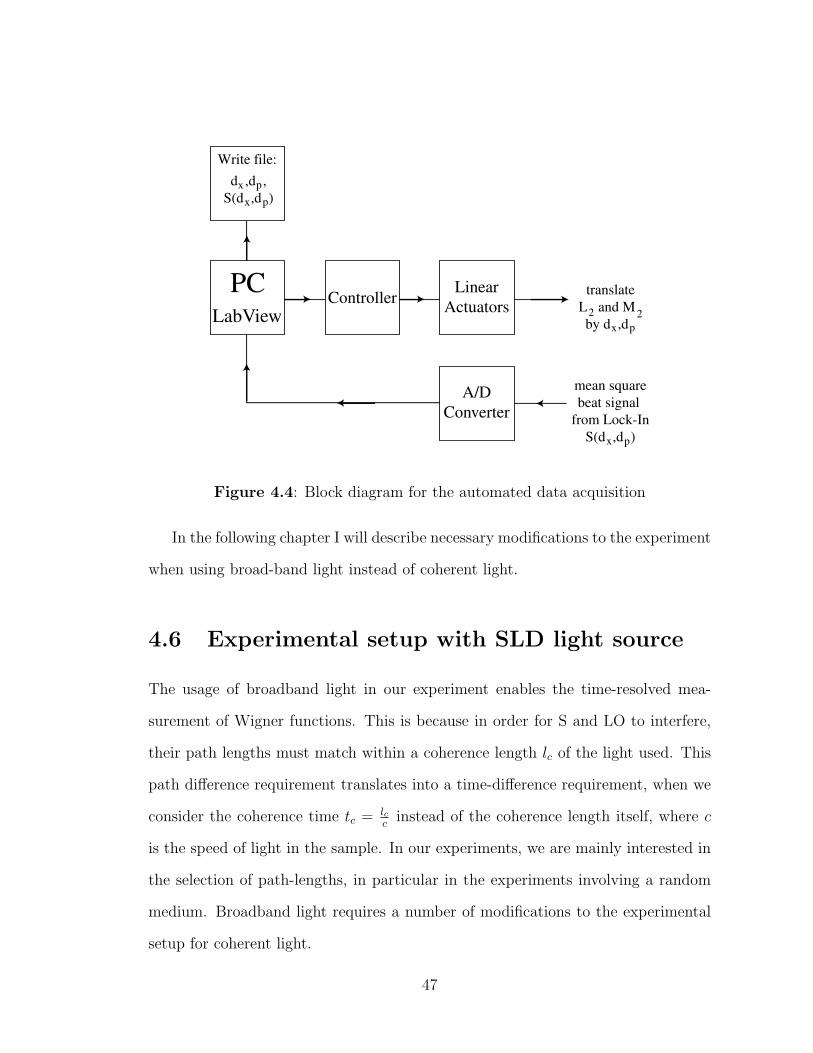
PC LabView

Controller Linear

Actuators

A/D Converter

translate L and M by d ,d 2 2

mean square beat signal

from Lock-In S(d ,d )px

x p

Write file:d ,d ,

S(d ,d )x p

x p

Figure 4.4: Block diagram for the automated data acquisition

In the following chapter I will describe necessary modifications to the experiment

when using broad-band light instead of coherent light.

4.6 Experimental setup with SLD light source

The usage of broadband light in our experiment enables the time-resolved mea-

surement of Wigner functions. This is because in order for S and LO to interfere,

their path lengths must match within a coherence length lc of the light used. This

path difference requirement translates into a time-difference requirement, when we

consider the coherence time tc = lcc

instead of the coherence length itself, where c

is the speed of light in the sample. In our experiments, we are mainly interested in

the selection of path-lengths, in particular in the experiments involving a random

medium. Broadband light requires a number of modifications to the experimental

setup for coherent light.

47

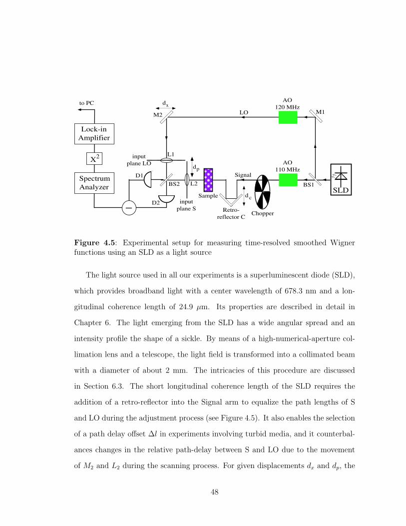
D1

M2

L2

L1

dx

dp

LO

Retro- reflector C

dc

X2

Spectrum Analyzer

Lock-in Amplifier

to PC

D2

Signal

AO 120 MHz

AO 110 MHz

Chopper

BS2

Sample

M1

BS1

SLDinput

plane S

input plane LO

Figure 4.5: Experimental setup for measuring time-resolved smoothed Wignerfunctions using an SLD as a light source

The light source used in all our experiments is a superluminescent diode (SLD),

which provides broadband light with a center wavelength of 678.3 nm and a lon-

gitudinal coherence length of 24.9 µm. Its properties are described in detail in

Chapter 6. The light emerging from the SLD has a wide angular spread and an

intensity profile the shape of a sickle. By means of a high-numerical-aperture col-

limation lens and a telescope, the light field is transformed into a collimated beam

with a diameter of about 2 mm. The intricacies of this procedure are discussed

in Section 6.3. The short longitudinal coherence length of the SLD requires the

addition of a retro-reflector into the Signal arm to equalize the path lengths of S

and LO during the adjustment process (see Figure 4.5). It also enables the selection

of a path delay offset ∆l in experiments involving turbid media, and it counterbal-

ances changes in the relative path-delay between S and LO due to the movement

of M2 and L2 during the scanning process. For given displacements dx and dp, the

48

correction will be given by the last three terms of Eq. (4.5):

∆l = 2dc + dx +d2

p

2f− dpdx

2f(4.5)

f is the focal length of the detector input lenses L1 and L2. The derivation of this

correction factor is outlined in the following section Section 4.7.

4.7 Measurement of smoothed Wigner functions

In this section I will describe how smoothed Wigner functions can be measured

using the experimental setup outlined in the previous section. The calculations will

be done for the more general case of partially coherent light of a broadband source,

since this light is used in all our experiments. The expressions for coherent light can

usually be directly deduced from those for partially coherent light. In most cases

they simplify considerably. In other parts of the calculation, I use transformations

for partially coherent light usually reserved for coherent light, but only when the

frequency dependency of the elements involved is negligible (lenses, short distances

of free space). The calculation of the squared beat signal and its connection to the

Wigner function of the Signal field will be the center part of this section. During

the calculation, the path-delay compensation necessary for broadband light and to

be performed by the retro-reflector will become evident.

For the following calculations, Figure 4.6 shows the notation regarding the dif-

ferent planes under consideration. The subscript 0 denotes the field right before the

input lens in the input plane, the prime ′ the field right behind it. The subscript D

denotes the field at the location of the detector.

In the derivation of the voltage output of the balanced detection scheme in

49

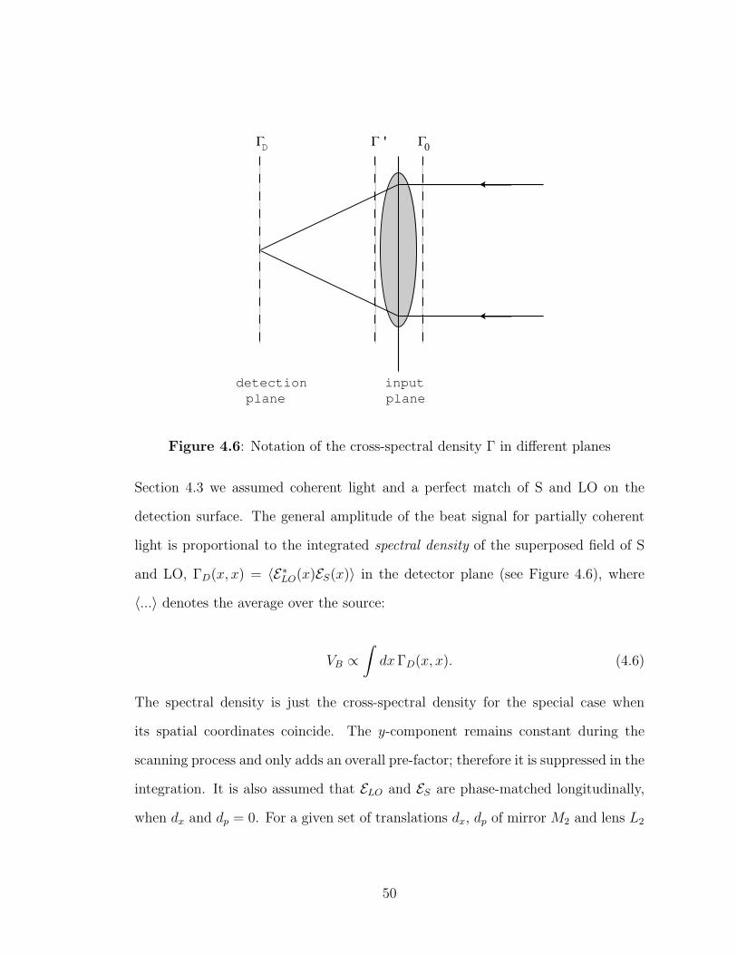
input plane

ΓΓ 0

ΓD '

detection plane

Figure 4.6: Notation of the cross-spectral density Γ in different planes

Section 4.3 we assumed coherent light and a perfect match of S and LO on the

detection surface. The general amplitude of the beat signal for partially coherent

light is proportional to the integrated spectral density of the superposed field of S

and LO, ΓD(x, x) = 〈E∗LO(x)ES(x)〉 in the detector plane (see Figure 4.6), where

〈...〉 denotes the average over the source:

VB ∝∫

dx ΓD(x, x). (4.6)

The spectral density is just the cross-spectral density for the special case when

its spatial coordinates coincide. The y-component remains constant during the

scanning process and only adds an overall pre-factor; therefore it is suppressed in the

integration. It is also assumed that ELO and ES are phase-matched longitudinally,

when dx and dp = 0. For a given set of translations dx, dp of mirror M2 and lens L2

50

the input fields ES, ELO right behind the input lenses are1

E ′∗LO(x) = E∗LO(x− dx) exp

(−i

k

2fx2

)(4.7)

E ′S(x) = ES(x) exp

[−i

k

2f(x− dp)

2

]. (4.8)

The first term in Eq. (4.7) is due to the translation of M2 which shifts the LO

relative to S by a distance dx. The following position dependent phase factor is the

paraxial approximation for the wavefront passed through input lens L1. A similar

transformation occurs in Eq. (4.8): S itself does not translate, but its input lens

L2 does by a factor dp, thereby introducing a position dependent quadratic phase

factor, shifted by dp. Even though ES and ELO superpose only in the beam splitter

and not yet in the input planes, we treat the problem as such in the following,

because we consider the input planes of the detection system as our reference. This

is perfectly valid, since both ES and ELO undergo the same linear transformations

after the input planes and before they superpose at the detectors.

The cross-spectral density of the superposed field behind the input lens is then:

Γ′(x, x′) = 〈E ′∗LO(x)E ′S(x′)〉 (4.9)

= Γ0(x− dx, x′) exp

i

k

2f[x2 − (x′ − dp)

2]

, (4.10)

where Γ0(x − dx, x′) = 〈E∗LO(x − dx)ES(x′)〉 is the cross-spectral density before the

1Since the SLD light is partially coherent, the cross-spectral density Γ(x1, x2) should actuallybe used instead of E(x). But, as pointed out at the beginning of this section, in cases where thecoherence properties have a negligible effect, I treat the field as if it were coherent since it simplifiesthe calculations.

51

lens. From there, both fields travel a distance f to the photodiodes, where f is

the focal length of the input lenses. The cross-spectral density at that location

can be calculated by propagating the cross-spectral density of ES and ELO with the

point-spread function for travel through free space (see Equations (3.9), (3.14)):

ΓD(x1, x′1) =

∫ ∫dx dx′ hxx(x1, x) Γ′(x, x′) h∗xx(x

′1, x

′) (4.11)

where, according to Eq. (3.14),

hxx(x1, x0) =

√k

2πizexp

[ik

2z(x1 − x0)

2

]. (4.12)

By inserting Equations (4.9) and (4.12) into Eq. (4.11), the cross-spectral density

at the detector results:

ΓD(x, x′) =k

2πfexp

[ik

2f(x2 − x′2 − d2

p)

]

×∫ ∫

dη dη′ Γ0(η − dx, η′)

× exp

ik

f[η2 − η′2 − x(η − η′) + η′dp]

. (4.13)

Inserting Eq. (4.13) into Eq. (4.6), the complex beat voltage for partially coherent

light results:

VB ∝ exp(−ik

2fd2

p)

∫dη Γ0(η − dx, η) exp(i

k

fηdp). (4.14)

The phase factors are due to path contributions when dp is off-center. They indicate

an additional path delay of

52

l′ = − d2p

2f+

dpη

f(4.15)

during the integration which introduces an attenuation factor of exp(− l′lc) due to

the short coherence length lc of the light source. By compensating those path delays

by means of the retro-reflector, the attenuating term vanishes. The second term in

Eq. (4.15) can not be compensated directly since it changes with integration over

the detector plane, but it can be minimized for certain types of fields. For signal

fields which are broad in position, as is the case for fields emerging from a turbid

medium, Γ(η − dx, η) is centered around dx. The phase factor inside the integral

in Eq. (4.14) can then be approximated by replacing η with dx, which results in a

correction factor

− d2p

2f+

dpdx

f. (4.16)

Another path delay that needs to be taken into consideration is introduced by the

translation of M2 by dx. Together with Eq. (4.16) the total correction term amounts

to

2dc = dx −d2

p

2f+

dpdx

f. (4.17)

The factor 2 in front of dc accounts for the fact that for a translation dc of the retro-

reflector the path length changes by 2dc, as can easily be seen. The attenuation due

to the varying path difference is now reduced to almost zero and the mean square

voltage is

| VB(dx, dp) |2∝∣∣∣∣∫

dη Γ0(η − dx, η) exp(ik

fηdp)

∣∣∣∣2

(4.18)

53

4.7.1 Mean square beat signal for transversely coherent light

For longitudinally coherent light, S and LO will interfere regardless of relative path

length difference. No correction by the retro-reflector is necessary. For transversely

coherent light, Γ0 separates into a product of E∗LO and ES due to the infinite trans-

verse coherence length (see Eq. (3.2)):

ΓCoh0 (x1, x2) = E∗LO(x1)ES(x2) (4.19)

without the requirement to average over fluctuations inherent only to partially co-

herent light, so that Eq. (4.18) can be written as

| V cohB (dx, dp) |2 ∝

∣∣∣∣∫

dη E∗LO,0(η − dx)ES,0(η) exp(−ik

fηdp)

∣∣∣∣2

=

∫dη E∗LO,0(η − dx)ES,0(η) exp(−i

k

fηdp)

×∫

dη′ ELO,0(η′ − dx)E∗S,0(η

′) exp(ik

fη′dp). (4.20)

In the following we replace η and η′ by the relative coordinates x = 12(η + η′) and

x′ = η− η′. The Jacobian in this case is unity, so dη dη′ = dx dx′. The substitution

yields:


∫dx

∫dx′ E∗LO,0(x +

x′

2− dx))ELO,0(x− x′

2− dx)

× E∗S,0(x +x′

2)ES,0(x− x′

2) exp(−i

k

fdpx

′). (4.21)

A product of fields E∗(x + ε2)E(x − ε

2) can be expressed in terms of their Wigner

54

function by inverse Fourier-transformation of expression Eq. (3.1):

E∗(x +ε

2)E(x− ε

2) =

∫dp exp(−iεp) W (x, p). (4.22)

Replacing E∗S,0(x + x′2)ES,0(x− x′

2) in Eq. (4.21) yields


∫dx

∫dx′ E∗LO,0(x +

x′

2− dx)ELO,0(x− x′

2− dx)

×∫

dp exp(ix′p) WS(x, p) exp(−ik

fdpx

′) (4.23)

where WS(x, p) is the Wigner function of the Signal field.

Using Eq. (3.1) again, we can express the remaining terms in Eq. (4.23) together

with the integral over dx′ as a Wigner function:

WLO(x0 − dx, p +k

fdp) =

∫dx′

2πexp[ix′(p +

k

fdp)]

× E∗LO,0(x +x′

2− dx)ELO,0(x− x′

2− dx). (4.24)

Replacing this expression in Eq. (4.23) we get as a final expression for the mean

square beat signal for coherent light:

| V cohB (dx, dp) |2∝

∫dx dp WLO(x− dx, p + px) WS(x, p) (4.25)

with px = kfdp.

This is a convolution of the Wigner functions of the Signal- and the Local Oscilla-

tor field which shows that the measured distribution is indeed a smoothed Wigner

55

function. For identical Signal- and Local Oscillator beams, such a convolution

broadens the phase-space profile by a factor√

2, as can easily be verified (also see

Section 5.4.4). For a finite transverse coherence length Γ0 does not separate into ELO

and ES; in that case | VB(dx, dp) |2 can not be expressed in terms of the individual

Wigner functions as in Eq. (4.25).

4.7.2 Averaging over fields

There are several types of averaging of interest in our experiments. First, there is

the averaging process in the Lock-In amplifier which extracts a weak signal from a

noisy background. Secondly, for experiments involving turbid media, the signal field

displays speckle, which are due to the interference of parts of the field taking different

paths in the medium. This effect is noticeable stronger for coherent light than for

partially coherent light. Speckle is considered noise in the type of experiments

we do and can shield weaker features of the field we are interested in. In our

experiment, we use polystyrene spheres floating in a water-glycerol mixture as a

turbid medium (see Section 12.1.1). These spheres are subject to Brownian motion;

therefore the speckle pattern changes with time. By ensemble averaging over the

sample, i.e. either spatial or temporal averaging over the signal field emerging

from the sample, speckle average out. Ensemble averaging in turbid media is also

necessary to make sure all possible arrangements of scatterers contribute to the

measured signal. The different techniques we apply for spatial averaging will be the

subject of Section 12.1.1. Temporal averaging is performed by the Lock-In amplifier

in our experiment. Ensemble averaging over a turbid medium is necessary for both

coherent and incoherent light probing the sample. For coherent light, it is often

more convenient to calculate the Wigner function of the ensemble averaged Signal

56

field and the LO field separately and use Eq. (4.25) to calculate the mean square

beat signal.

For partially coherent light on the other hand, a third type of averaging makes it

necessary to perform the averaging at the plane where S and LO interfere: Partially

coherent light of frequency ω, which has a bandwidth of ∆ω, fluctuates temporally

at a rate of about ∆ω. In our experiment we measure the average of the fluctuating

product of S and LO which is not equal to the product of the averaged S and LO

itself, at least for partially coherent light:

〈E∗LOES〉 6= 〈E∗LO〉〈ES〉 (4.26)

4.7.3 Resolution of the Single-Window technique

The resolution of the measured signal field is determined by the size of the LO in

phase-space, namely its spatial width and its angular spread. For a Gaussian beam

with a diameter of 2σs the angular spread is about λ2σs

, i.e. ∆k = 12σs

, so that

∆x∆k = 1.

There is obviously a trade-off between good position- and momentum resolution:

A small diameter σs of the LO provides good position resolution, but its resulting

high momentum spread decreases the momentum resolution. The opposite relation-

ship holds for a wide collimated beam. This uncertainty relation associated with

Fourier transform pairs can be surpassed by using a combination of two LOs with

small and big diameter, as will be described in the next chapter.

57

Chapter 5

The Two-Window technique

5.1 Introduction

The last chapter which treated the experimental setup for the Single-Window tech-

nique showed that there is a trade-off between position and momentum resolution if

a single LO is used. Therefore, the measured signal is a smoothed Wigner function

rather then the true Wigner function. In the following, we present a Two-Window

technique which employs a combination of two phase-coupled LOs, which enables

the measurement of un-smoothed Wigner functions. The set of phase-coupled LOs

consists of an LO which is narrowly focused to allow high spatial resolution (small

LO or SLO), and a second LO which is highly collimated which provides high angu-

lar resolution (big LO or BLO). Both LOs are frequency-shifted by 120 and 120.003

MHz, respectively; their frequency-difference of 3 kHz is locked to an external oscil-

lator by means of a phase-locked loop. The signal field S, which is frequency-shifted

by 110 MHz as in the Single-Window experimental setup, is superposed with the

dual-LO in the detector plane. This time, the beat note contains two frequency

components, one from the superposition of S and BLO at 10 MHz, the other from

S and SLO at 10.003 MHz.

The beat-signals are detected by a spectrum analyzer and squared as in the

58

Single-Window case. The signal exiting the squarer oscillates at the frequency

difference of SLO and BLO of 3 kHz and is detected in the Lock-In amplifier which

uses the 3 kHz external oscillator as a reference. The quadrature outputs of the

Lock-In amplifier contain all the information about the true Wigner function, as we

will see below.

In the following section, the experimental setup for the Two-Window technique

will be described. In Section 5.3 and Section 5.3.1 we will derive the mathematical

expression for the signal we measure and show how to retrieve the true Wigner

function of the field from it. Also, a derivation of the direct relation between mean

square beat signal and the distribution of the Signal field in position and momentum

will be presented. In Section 5.4 we discuss the physical meaning of the measured

complex beat-signal for an ideal and non-ideal dual-LO.

I will conclude the chapter by short descriptions of the Acousto-optic modulators

(Section 5.5), the phase-locked loop I developed for this experiment (Section 5.6),

the 4f -system (Section 5.7), and an overview over the complete system (Section 5.8).

5.2 Experimental Setup

As already mentioned in the Introduction, the Two-Window technique employs a

pair of phase-coupled LO’s instead of a single LO as in the Single-Window case.

This pair consists of a large collimated beam (’Big LO’ or BLO) providing high

momentum resolution and a small focused beam (’Small LO’ or SLO) providing

high spatial resolution. Figure 5.1 shows the experimental setup. Again, a 4f -

system as well as other optical components which are not crucial for grasping the

concept of this technique were omitted in the figure. Electronic connections are

displayed as dashed lines, optical pathways as solid lines. While the Signal arm has

59

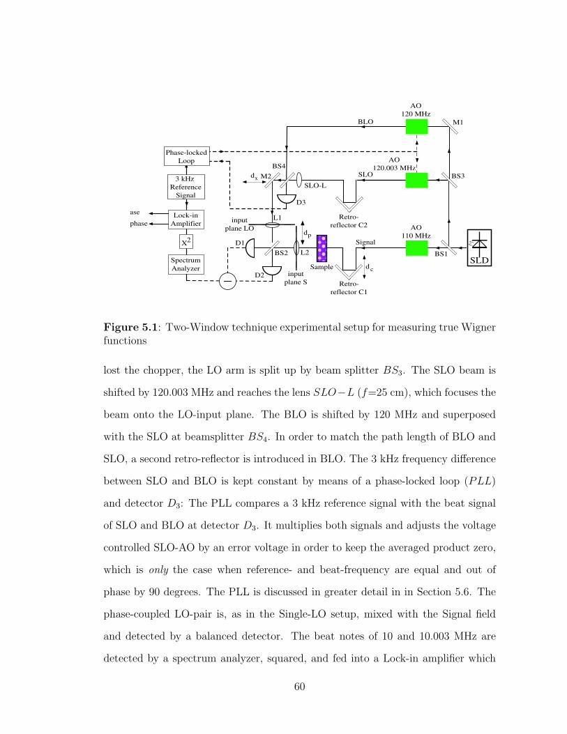
D1

M2

L2

L1

dx

dp

SLO

Retro- reflector C1

dc

X2

Spectrum Analyzer

Lock-in Amplifier

D2

Signal

AO 120.003 MHz

AO 110 MHz

BS2

Sample

M1

BS1SLD

input plane S

input plane LO

AO 120 MHz

BS3BS4

SLO-L3 kHz

Reference Signal

D3

BLO

Phase-locked Loop

Retro- reflector C2

In-phase

Out-of-phase

Figure 5.1: Two-Window technique experimental setup for measuring true Wignerfunctions

lost the chopper, the LO arm is split up by beam splitter BS3. The SLO beam is

shifted by 120.003 MHz and reaches the lens SLO−L (f=25 cm), which focuses the

beam onto the LO-input plane. The BLO is shifted by 120 MHz and superposed

with the SLO at beamsplitter BS4. In order to match the path length of BLO and

SLO, a second retro-reflector is introduced in BLO. The 3 kHz frequency difference

between SLO and BLO is kept constant by means of a phase-locked loop (PLL)

and detector D3: The PLL compares a 3 kHz reference signal with the beat signal

of SLO and BLO at detector D3. It multiplies both signals and adjusts the voltage

controlled SLO-AO by an error voltage in order to keep the averaged product zero,

which is only the case when reference- and beat-frequency are equal and out of

phase by 90 degrees. The PLL is discussed in greater detail in in Section 5.6. The

phase-coupled LO-pair is, as in the Single-LO setup, mixed with the Signal field

and detected by a balanced detector. The beat notes of 10 and 10.003 MHz are

detected by a spectrum analyzer, squared, and fed into a Lock-in amplifier which

60

uses the 3 kHz reference signal as a reference as opposed to the chopper used in

the Single-Window setup. The Lock-in amplifier produces two quadrature voltages:

an In-phase signal which is proportional to the signal component which is in phase

with respect to the reference signal, and an out-of-phase signal which is proportional

to the component which is 90 degrees shifted to it. In combination they contain

the complete amplitude- and phase information of the detected signal. In the next

section I show how the true Wigner function of a signal field can be measured using

this setup.

5.3 Measurement of true Wigner functions

For sufficiently high global coherence, the Wigner function of a Signal field can be

directly measured. In our experiment, this condition is met to a very good degree

with a global coherence of more than 7 (see Section 8.1). In the following we show

how the true Wigner function is measured and retrieved.

The LO in the dual-LO scheme is a phase-coupled pair of a small LO (SLO) and

a big LO (BLO), as already mentioned. Its electric field can be written as: 1

ELO(x) = ELO,0

[exp(− x2

2a2) + βeiωt exp(− x2

2A2)

], (5.1)

where eiωt denotes the relative phase of the BLO with respect to the SLO determined

by the phase-locking at ω = 2π×3 kHz and β its relative amplitude. a and A are the

beam intensity e−2 radii for the SLO and BLO, respectively. The Wigner function

for this LO is then:

1In the following calculation, a and A denote characteristic widths of SLO and BLO. In allother calculations in this thesis a and A are dimensionless scaling factors. We only choose to strayfrom this habit here to enhance the readability of the formulae.

61

WLO(x, p) =

∫dε

2πeipεE∗LO(x +

ε

2)ELO(x− ε

2)

= E2LO,0

∫dε

2πeipε

exp

[−(x + ε

2)2

2a2

]+ βe−iωt exp

[−(x + ε

2)2

2A2

]

×

exp

[−(x− ε

2)2

2a2

]+ βeiωt exp[−(x− ε

2)2

2A2]

. (5.2)

Since the Lock-in amplifier locks on to the reference frequency used to phase-lock

the LO’s, only the cross terms ∝ exp(±iωt) in Eq. (5.2) are detected; the other

terms cancel. The cross terms are

WaA(x, p) = βE20

∫dε

2πeipε

eiωt exp

[−(x + ε

2)2

2a2− (x− ε

2)2

2A2

]

+ e−iωt exp

[−(x + ε

2)2

2A2− (x− ε

2)2

2a2

]

∝ e−iωtI + eiωtI∗ (5.3)

where

I =

∫dε

2πexp

[−(x + ε

2)2

2a2− (x− ε

2)2

2A2

]eiεp. (5.4)

I can be transformed the following way:

62

I =

∫dε

2πexp

[−A2(x + ε

2)2 + a2(x− ε

2)2

2a2A2

]eiεp

=

∫dε

2πexp

−1

2

[(

1

a2+

1

A2)(x2 +

ε2

4) + (

1

a2− 1

A2)xε

]eiεp

= exp

[−1

2(

1

a2+

1

A2)x2

]

×∫

dε

2πexp

−

[1

8(

1

a2+

1

A2)ε2 +

1

2(

1

a2− 1

A2)xε− ipε

]

= exp(−α

2x2)

∫dε

2πexp

[−

(α

8ε2 +

β

2xε− ipε

)](5.5)

where

α =1

a2+

1

A2

β =1

a2− 1

A2. (5.6)

Solving the integral in Eq. (5.5) yields:

I =4

αexp(−α

2x2) exp

[2

α

(β2

4x2 − p2 − iβxp

)]

=4

αexp

[−(

α

2− β2

2α)x2 − 2

αp2 − 2i

β

αxp

]. (5.7)

Replacing α and β according to Eq. (5.6), one gets

I ∝ A2a2

A2 + a2exp

(−2x2 1

A2 + a2− 2p2 A2a2

A2 + a2− 2i

A2 − a2

A2 + a2xp

)(5.8)

which reduces to

63

I ∝ exp

(−2x2

A2− 2a2p2 − 2ixp

)(5.9)

for A À a. This is always the case in our experiment, where we choose the BLO to

have a much larger diameter than the focused SLO. When we choose the diameters

of BLO and SLO so that A is much bigger than the position x range of the Signal

field and 1a

much bigger than the momentum p range of the Signal field we measure,

the exponential terms in Eq. (5.9) reduce to unity and we get:

I ∝ exp(−2ixp). (5.10)

With Equations (5.9) or (5.10) we can calculate the Wigner function of the LO in

Eq. (5.3):

WaA(x, p) ∝ e−iωtI + eωtI∗

= exp

(−2x2

A2− 2a2p2

)[exp(iωt− 2ixp) + exp(−iωt + 2ixp)]

= 2 exp

(−2x2

A2− 2a2p2

)cos(2xp− ωt) (5.11)

≈ 2 cos(2xp− ωt). (5.12)

Now that we have the Wigner function for our dual-LO beam, we can calculate the

in-phase signal we measure, using Eq. (4.25)

SIPB (x, p) =

∫dx′ dp′ WLO(x′ − x, p′ − p) WS(x′, p′)

∝∫

dx′ dp′ cos[2(x′ − x)(p′ − p)] WS(x′, p′). (5.13)

64

The second quadrature of the Lock-In amplifier, which is referred to as out-of-

phase signal, measures the signal field component that is 90 degrees out of phase

with respect to the reference signal and can be found by subtracting a phase of 90

degrees from ωt in Eq. (5.13). This manipulation just changes cosine into sine:

SOPB (x, p) ∝

∫dx′ dp′ sin[2(x′ − x)(p′ − p)] WS(x′, p′). (5.14)

The combined in-phase and out-of-phase signals can be written more elegantly using

complex notation:

SB(x, p) = SIPB (x, p) + iSOP

B (x, p) (5.15)

=1

π

∫dx′ dp′ exp[2i(x′ − x)(p′ − p)] WS(x′, p′). (5.16)

S(x, p) is a Margenau-Hill transformation of the true Wigner function WS(x, p) of

the field. We will refer to SB(x, p) as the complex beat signal.

5.3.1 Extraction of the true Wigner function from SB(x, p)

In order to retrieve the Wigner function WS(x′, p′) of the signal field, the expression

in Eq. (5.16) must be inverted. A reasonable guess would be that

WS(x, p) =1

π

∫dx′ dp′ exp[−2i(x− x′)(p− p′)] SB(x′, p′). (5.17)

That this is indeed the case can be shown very straightforwardly by integrating Eq.

(5.16) from both sides according to the right side of Eq. (5.17):

65

1

π

∫dx dp SB(x, p) exp[−2i(x′′ − x)(p′′ − p)]

=1

π2

∫ ∫ ∫ ∫dx dp dx′ dp′ exp[−2i(x′′ − x)(p′′ − p) + 2i(x′ − x)(p′ − p)]

× WS(x′, p′)

=1

π2

∫ ∫ ∫ ∫dx dp dx′ dp′ exp[2i(x′p′ − x′′p′′ + x(p′′ − p′) + p(x′′ − x′)]

× WS(x′, p′)

=1

π2

∫ ∫exp[2i(x′p′ − x′′p′′)] WS(x′, p′)

×∫

dx dp exp[2i(x(p′′ − p′) + p(x′′ − x)]. (5.18)

The last integral on the left reduces to a product of delta functions:

∫dx dp exp[2i(x(p′′ − p′) + p(x′′ − x)] = π2δ(p′′ − p′)δ(x′′ − x′) (5.19)

so that Eq. (5.18) becomes:

π2 1

π2

∫ ∫exp[2i(x′p′ − x′′p′′)] WS(x′, p′)δ(p′′ − p′)δ(x′′ − x′)

= WS(x′′, p′′). (5.20)

Summarizing Equations (5.18)-(5.20), it was shown that WS(x, p) can indeed be

retrieved from the complex beat signal SB(x, p) by means of the inverse Margenau-

Hill transformation

66

WS(x, p) =1

π

∫dx′ dp′ exp[−2i(x− x′)(p− p′)] SB(x′, p′). (5.21)

Eq. (5.21) shows that the Two-Window technique enables the retrieval of the true

Wigner function without the smoothing effect of a convolution with the Wigner

function of a Single-LO. The spatial and momentum resolution with which the

Wigner function is measured is limited by the size of the small LO and collimation

of the big LO.

In practice, we use a C++ program program to perform the inverse Margenau-

Hill transformation in Eq. (5.21) for the data we measure. The program code and

description can be found in Appendix C.

5.3.2 Relation between SB(x, p) and the Signal field

Another interesting relation between the measured complex beat signal SB(x, p)

and the Signal field as a function of position and momentum will be demonstrated

in the following.

When we replace WS(x, p) in Eq. (5.16) by its expression in terms of the cross-

spectral density in Eq. (3.1), we get

67

SB(x, p) =1

π

∫dx′ dp′ exp[2i(x′ − x)(p′ − p)]

×∫

dε exp(iεp) 〈E∗(x′ + ε

2) E(x′ − ε

2)〉

=1

π

∫dx′

∫dε 〈E∗(x′ + ε

2) E(x′ − ε

2)〉

×∫

dp′ exp(iεp′) exp[2i(x′ − x)(p′ − p)]

=1

π

∫dx′

∫dε 〈E∗(x′ + ε

2) E(x′ − ε

2)〉

× exp[2i(x− x′)p]

∫dp′ exp(iεp′) exp[2i(x′ − x)p′]. (5.22)

The last integral in Eq. (5.22) reduces to a delta function:

∫dp′ exp(iεp′) exp[2i(x′ − x)p′] = 2πδ[ε + 2(x′ − x)] (5.23)

so that Eq. (5.22) becomes

SB(x, p) = 2〈E∗(x) exp(2ixp)

∫dx′ E(2x′ − x) exp(−2ix′p)〉. (5.24)

If we replace 2x′ − x by the variable u, Eq. (5.24) becomes:

SB(x, p) = 〈E∗(x) exp(2ixp)

∫du E(u) exp[−i(u + x)p] 〉

= 〈E∗(x) exp(ixp)

∫du E(u) exp(−iup)〉

= 〈E∗(x) E(p)〉 exp(ixp). (5.25)

The measured signal SB(x, p) is the averaged correlation of the Signal field at a given

68

position E(x) and the Signal field at given momentum E(p), times a phase-factor. A

much shorter derivation in terms of the electric fields as well as a discussion of the

phase-factor will be given in Section 5.4. We note that this expression only holds

for Signal fields which are sufficiently broad in space and momentum, which is the

case for all our experiments involving turbid media. In other words, the results for

an ideal Dual-LO must be very close to those for the Dual-LO we employ. In our

experiments involving the characterization of the Signal beam itself, we have to take

into account the finite size of the BLO and the non-zero size of the SLO we use.

This will be discussed for a transverse coherent beam in Section 5.4.3; the complete

derivation for a finite coherence area of a beam will be performed in Section 7.2.

5.4 Interpretation of the measured beat signals

In the Two-window scheme, the balanced detection system isolates two beat notes

from the frequency components of ES, EBLO and ESLO which oscillate with 110, 120

and 120.003 MHz. Between the SLO and BLO, there is no 180 degree phase-shift

since they take the same paths through the detector beam splitter. Therefore, their

beat amplitude at a relative frequency of 3 kHz cancels in the balanced detector.

The relative phase-shift exists only between the Signal field on one side and the SLO

and BLO on the other side. The measured beat notes have therefore frequencies

of 10 and 10.003 MHz. The bandwidth on the spectrum analyzer has to be chosen

so that both frequencies can pass without experiencing attenuation or frequency-

dependent phase-shifts. In our experiment, the bandwidth was set to at least ten

times the frequency difference.

The beat note of a superposed LO and S can be written as (see Eq. (4.6)):

69

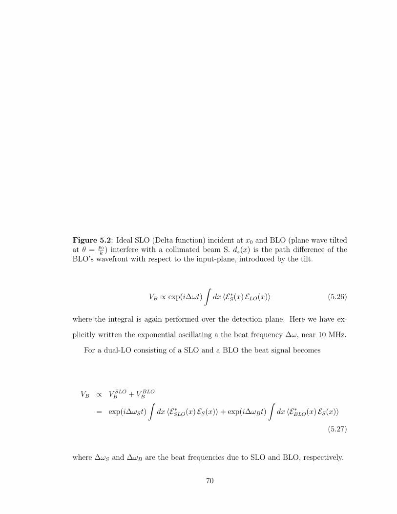
θ

SLO

BLO

d (x)z

xx0

0

d (0)z

Collimated Gaussian beam S

input plane

Figure 5.2: Ideal SLO (Delta function) incident at x0 and BLO (plane wave tiltedat θ = p0

k) interfere with a collimated beam S. dz(x) is the path difference of the

BLO’s wavefront with respect to the input-plane, introduced by the tilt.

VB ∝ exp(i∆ωt)

∫dx 〈E∗S(x) ELO(x)〉 (5.26)

where the integral is again performed over the detection plane. Here we have ex-

plicitly written the exponential oscillating a the beat frequency ∆ω, near 10 MHz.

For a dual-LO consisting of a SLO and a BLO the beat signal becomes

VB ∝ V SLOB + V BLO

B

= exp(i∆ωSt)

∫dx 〈E∗SLO(x) ES(x)〉+ exp(i∆ωBt)

∫dx 〈E∗BLO(x) ES(x)〉

(5.27)

where ∆ωS and ∆ωB are the beat frequencies due to SLO and BLO, respectively.

70

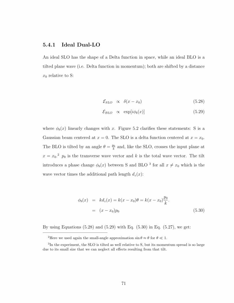
5.4.1 Ideal Dual-LO

An ideal SLO has the shape of a Delta function in space, while an ideal BLO is a

tilted plane wave (i.e. Delta function in momentum); both are shifted by a distance

x0 relative to S:

ESLO ∝ δ(x− x0) (5.28)

EBLO ∝ exp[iφb(x)] (5.29)

where φb(x) linearly changes with x. Figure 5.2 clarifies these statements: S is a

Gaussian beam centered at x = 0. The SLO is a delta function centered at x = x0.

The BLO is tilted by an angle θ = p0

kand, like the SLO, crosses the input plane at

x = x0.2 p0 is the transverse wave vector and k is the total wave vector. The tilt

introduces a phase change φb(x) between S and BLO 3 for all x 6= x0 which is the

wave vector times the additional path length dz(x):

φb(x) = kdz(x) = k(x− x0)θ = k(x− x0)p0

k.

= (x− x0)p0 (5.30)

By using Equations (5.28) and (5.29) with Eq. (5.30) in Eq. (5.27), we get:

2Here we used again the small-angle approximation sin θ ≈ θ for θ ¿ 1.3In the experiment, the SLO is tilted as well relative to S, but its momentum spread is so large

due to its small size that we can neglect all effects resulting from that tilt.

71

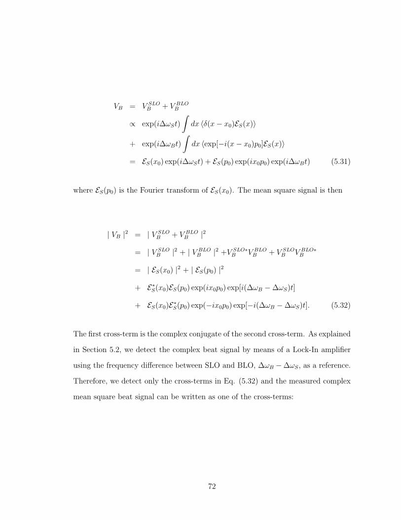
VB = V SLOB + V BLO

B

∝ exp(i∆ωSt)

∫dx 〈δ(x− x0)ES(x)〉

+ exp(i∆ωBt)

∫dx 〈exp[−i(x− x0)p0]ES(x)〉

= ES(x0) exp(i∆ωSt) + ES(p0) exp(ix0p0) exp(i∆ωBt) (5.31)

where ES(p0) is the Fourier transform of ES(x0). The mean square signal is then

| VB |2 = | V SLOB + V BLO

B |2

= | V SLOB |2 + | V BLO

B |2 +V SLO∗B V BLO

B + V SLOB V BLO∗

B

= | ES(x0) |2 + | ES(p0) |2

+ E∗S(x0)ES(p0) exp(ix0p0) exp[i(∆ωB −∆ωS)t]

+ ES(x0)E∗S(p0) exp(−ix0p0) exp[−i(∆ωB −∆ωS)t]. (5.32)

The first cross-term is the complex conjugate of the second cross-term. As explained

in Section 5.2, we detect the complex beat signal by means of a Lock-In amplifier

using the frequency difference between SLO and BLO, ∆ωB −∆ωS, as a reference.

Therefore, we detect only the cross-terms in Eq. (5.32) and the measured complex

mean square beat signal can be written as one of the cross-terms:

72

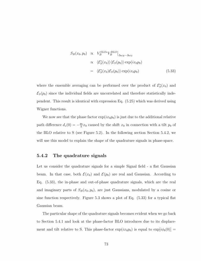
SB(x0, p0) ∝ V SLO∗B V BLO

B

∣∣∆ωB−∆ωS

∝ 〈E∗S(x0)〉〈ES(p0)〉 exp(ix0p0)

= 〈E∗S(x0)ES(p0)〉 exp(ix0p0) (5.33)

where the ensemble averaging can be performed over the product of E∗S(x0) and

ES(p0) since the individual fields are uncorrelated and therefore statistically inde-

pendent. This result is identical with expression Eq. (5.25) which was derived using

Wigner functions.

We now see that the phase factor exp(ix0p0) is just due to the additional relative

path difference dz(0) = −p0

kx0 caused by the shift x0 in connection with a tilt p0 of

the BLO relative to S (see Figure 5.2). In the following section Section 5.4.2, we

will use this model to explain the shape of the quadrature signals in phase-space.

5.4.2 The quadrature signals

Let us consider the quadrature signals for a simple Signal field - a flat Gaussian

beam. In that case, both E(x0) and E(p0) are real and Gaussian. According to

Eq. (5.33), the in-phase and out-of-phase quadrature signals, which are the real

and imaginary parts of SB(x0, p0), are just Gaussians, modulated by a cosine or

sine function respectively. Figure 5.3 shows a plot of Eq. (5.33) for a typical flat

Gaussian beam.

The particular shape of the quadrature signals becomes evident when we go back

to Section 5.4.1 and look at the phase-factor BLO introduces due to its displace-

ment and tilt relative to S. This phase-factor exp(ix0p0) is equal to exp[iφb(0)] =

73

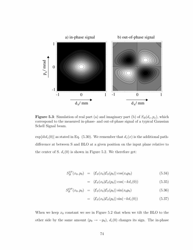
0 0

0

1 1-1

1

-1-1

p /

mra

dx

d / mmx d / mmx

a) in-phase signal b) out-of-phase signal

Figure 5.3: Simulation of real part (a) and imaginary part (b) of SB(dx, px), whichcorrespond to the measured in-phase- and out-of-phase signal of a typical GaussianSchell Signal beam.

exp[ikdz(0)] as stated in Eq. (5.30). We remember that dz(x) is the additional path-

difference at between S and BLO at a given position on the input plane relative to

the center of S. dz(0) is shown in Figure 5.2. We therefore get:

SIPB (x0, p0) = 〈ES(x0)ES(p0)〉 cos(x0p0) (5.34)

= 〈ES(x0)ES(p0)〉 cos(−kdz(0)) (5.35)

SOPB (x0, p0) = 〈ES(x0)ES(p0)〉 sin(x0p0) (5.36)

= 〈ES(x0)ES(p0)〉 sin(−kdz(0)) (5.37)

When we keep x0 constant we see in Figure 5.2 that when we tilt the BLO to the

other side by the same amount (p0 → −p0), dz(0) changes its sign. The in-phase

74

part does not see the sign of dz(0) here; its amplitude which is maximal for p0 = 0

becomes smaller in each case by the same amount. The out-of-phase signal on the

other hand which is proportional to the sine of −kdz(0), switches its sign. The same

happens when we keep the momentum of BLO constant and change the location

of the LOs from x0 to −x0, where dz(0) changes its sign as well. This behavior

of these phase-terms, together with the Gaussian dependence of the beat-signals

amplitude, explains the spade-like shape of the in-phase signal (Figure 5.3a) as well

as the clover-like appearance of the out-of-phase signal (Figure 5.3b).

5.4.3 Non-ideal Dual-LO

The requirements for an SLO to be infinitely small and a BLO to be a perfect

plane wave can of course not be realized. In fact, both SLO and BLO have a

Gaussian beam profile. While the SLO has a diameter of about 100 µm, the BLO has

approximately the same size as the Signal beam. As already mentioned, most Signal

fields measured in our experiment have position- and momentum distributions which

are much larger than those of the SLO or the BLO, respectively. In those cases,

the Dual-LO can be considered perfect, to a good approximation. When we try

do determine the beam parameters of the Signal input beam itself (Chapter 7) on

the other hand, we must take into account that its momentum distribution is equal

to that of the BLO and the BLO also becomes position-dependent due to its finite

size. The SLO on the other hand can still be considered perfect, with its beam size

smaller than the Signal beam by an order of magnitude.

In the following we will briefly outline the corrections for the beat signal of a

finite size BLO and a similar Signal beam. The expression for an ideal BLO on the

right of Eq. (5.29) is multiplied by a Gaussian term:

75

ErealBLO(x,A) ∝ exp[iφb(x)] exp(− x2

2A2) (5.38)

For an ideal BLO, A →∞ and the second exponential becomes unity. We express

the Signal beam in the Gaussian-Schell model as a product of a Gaussian term and

a phase term E ′S(x) describing the curvature of the field:

ES(x) ∝ exp(− x2

2B2)E ′S(x) (5.39)

B is usually on the order of half a millimeter. Again we assume the transverse

coherence length to be sufficiently large to be neglected. The beat signal for the

BLO in line 3 of Eq. (5.31) then becomes:

V realBLOB (x0, p0, A,B) ∝

∫dx exp[−i(x− x0)p0] exp[−(x− x0)

2

2A2] exp(− x2

2B2)E ′S(x)

∝ exp(ix0p0) exp[− x20

2(A2 + B2)]

×∫

dx exp(−ixp0) exp

[−1

2(

1

A2+

1

B2)(x− x0

1 + A2

B2

)2

]E ′S(x)

(5.40)

where we omitted the exponential containing the beat frequency which will not be

affected by the following calculations. There is no general solution to the above

integral. For a plane wavefront (E ′S(x) ≡ 1), Eq. (5.40) becomes

76

V realBLOB (x0, p0, A, B, R = ∞) ∝ exp

[− x2

0

2(A2 + B2)

]exp

[− p2

0

2( 1A2 + 1

B2 )

]

× exp

[ix0p0

(1

1 + B2

A2

)]. (5.41)

Compared to the the beat signal for an ideal BLO (A →∞)

V idealBLOB (x0, p0, B, R = ∞) ∝ exp(−B2

2p2

0) exp(ix0p0) (5.42)

the pre-factor of both x0 and p0 change by a factor√

1 + B2

A2 , as can easily be seen:

V realBLOB (x0, p0, A, B, R = ∞) = V idealBLO

B (x0√

1 + B2

A2

,p0√

1 + B2

A2

, R = ∞). (5.43)

In our experiment, B = A, so Eq. (5.43) reduces to:

V realBLOB (x0, p0, A = B, R = ∞) = V idealBLO

B (x0√2,

p0√2, R = ∞) (5.44)

which is the expected result for the convolution of two equal-sized beams, as in the

Single-LO technique. The above expressions is only exact for R = ∞; for finite R

we need to replace 12B2 by 1

2B2 − ik2R

= 12B2 (1 − ikB2

R). Eq. (5.44) is still a good

approximation as long as R À kB2 which is usually on the order of 5 meters.

For completeness we mention the result for V realBLOB for the other extreme where

the radii of curvature R ¿ kB2:

77

V realBLOB (x0, p0, A, B,Rsmall) ∝ exp

[− 1

2A2(x0 − R

kp0)

2 − R2

2B2k2p2

0

]

× exp

i

[xp +

2R

k

(x2

(2A2)2+ p2

)](5.45)

The derivation is shown in Appendix B.

5.4.4 Measurement of Gaussian beams for ideal and real

Dual-LO

While a real Dual-LO comes very close to an ideal LO in most experiments involving

turbid media, in measurements of Signal fields which are small in phase-space the

true properties of BLO and SLO have to be taken into account. For a flat Gaussian

Signal field of the form

ES(x) ∝ exp(− x2

2B2), (5.46)

an ideal Dual-LO will measure a complex beat signal of

SidealB (x0, p0) ∝ ES(x0)ES(p0) exp(ix0p0)

∝ exp(− x2

2B2) exp(−B2

2p2) exp(ix0p0) (5.47)

as shown in Eq. (5.33), where we omitted the averaging brackets again since we

consider a transverse coherent beam. Also, the electric fields are real because the

wavefront is flat.

For the Dual-LO in our experiment on the other hand, which uses practically

78

an ideal SLO but a BLO the size of the Signal beam (A=B), the measured signal is

SrealB (x0, p0) = exp

[−x2

2

(1

B2+

1

A2 + B2

)]exp

(− B2

2( 1A2 + 1

B2 )p2

0

)

× exp

[ix0p0

(1− 1

1 + B2

A2

)]

= exp[− x2

2B2(23)] exp(−B2

4p2

0) exp(i

2x0p0). (5.48)

It can easily be seen that the measured position distribution is narrower by a factor√

23

compared to a perfect BLO, while the momentum distribution is broader by a

factor√

2 (convolution of two beams with identical momentum distribution).

In Chapter 7 we will characterize the Signal beam of the SLD we use, which re-

quires the incorporation of the finite transverse coherence length into the calculation

of the beat signals.

In the following I will give an overview over some of the integral building blocks

of the experimental setup.

5.5 Acousto-optic modulators (AO)

In our experiment we use three AO-Drivers and -crystals by IsoMET Co. with driver

shifting frequencies of 110 and 120 MHz and a third 120 MHz tunable-one. The

crystals are made from Lead Molybdate (PbMoO4) and have an active aperture of 1

mm. The tunable AO-driver contains a VCO with a voltage range between 4 and 17

V, which corresponds to a frequency range of 80 to 130 MHz. The frequency-voltage

dependency is approximately linear.

79

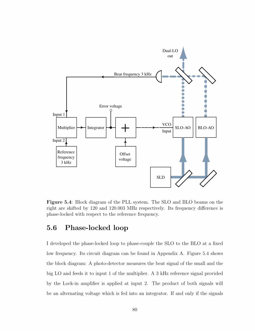
+Offset voltage

Reference frequency

3 kHz

Integrator SLO-AOVCO

InputBLO-AO

Beat frequency 3 kHz

Input 1

Input 2

Error voltage

SLD

Dual-LO out

Multiplier

Figure 5.4: Block diagram of the PLL system. The SLO and BLO beams on theright are shifted by 120 and 120.003 MHz respectively. Its frequency difference isphase-locked with respect to the reference frequency.

5.6 Phase-locked loop

I developed the phase-locked loop to phase-couple the SLO to the BLO at a fixed

low frequency. Its circuit diagram can be found in Appendix A. Figure 5.4 shows

the block diagram: A photo-detector measures the beat signal of the small and the

big LO and feeds it to input 1 of the multiplier. A 3 kHz reference signal provided

by the Lock-in amplifier is applied at input 2. The product of both signals will

be an alternating voltage which is fed into an integrator. If and only if the signals

80

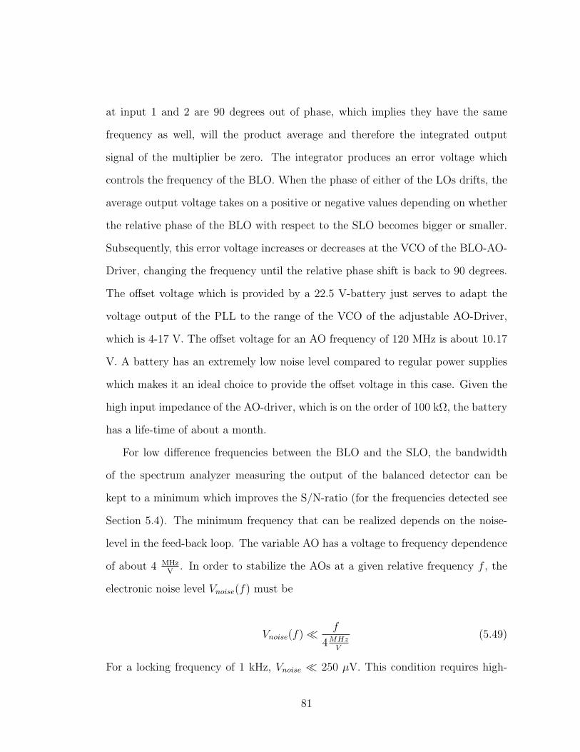
at input 1 and 2 are 90 degrees out of phase, which implies they have the same

frequency as well, will the product average and therefore the integrated output

signal of the multiplier be zero. The integrator produces an error voltage which

controls the frequency of the BLO. When the phase of either of the LOs drifts, the

average output voltage takes on a positive or negative values depending on whether

the relative phase of the BLO with respect to the SLO becomes bigger or smaller.

Subsequently, this error voltage increases or decreases at the VCO of the BLO-AO-

Driver, changing the frequency until the relative phase shift is back to 90 degrees.

The offset voltage which is provided by a 22.5 V-battery just serves to adapt the

voltage output of the PLL to the range of the VCO of the adjustable AO-Driver,

which is 4-17 V. The offset voltage for an AO frequency of 120 MHz is about 10.17

V. A battery has an extremely low noise level compared to regular power supplies

which makes it an ideal choice to provide the offset voltage in this case. Given the

high input impedance of the AO-driver, which is on the order of 100 kΩ, the battery

has a life-time of about a month.

For low difference frequencies between the BLO and the SLO, the bandwidth

of the spectrum analyzer measuring the output of the balanced detector can be

kept to a minimum which improves the S/N-ratio (for the frequencies detected see

Section 5.4). The minimum frequency that can be realized depends on the noise-

level in the feed-back loop. The variable AO has a voltage to frequency dependence

of about 4 MHzV

. In order to stabilize the AOs at a given relative frequency f , the

electronic noise level Vnoise(f) must be

Vnoise(f) ¿ f

4MHzV

(5.49)

For a locking frequency of 1 kHz, Vnoise ¿ 250 µV. This condition requires high-

81

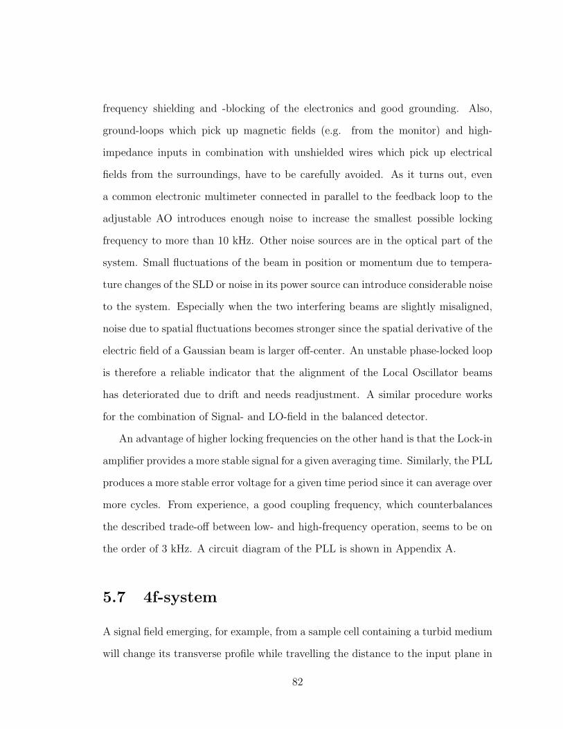
frequency shielding and -blocking of the electronics and good grounding. Also,

ground-loops which pick up magnetic fields (e.g. from the monitor) and high-

impedance inputs in combination with unshielded wires which pick up electrical

fields from the surroundings, have to be carefully avoided. As it turns out, even

a common electronic multimeter connected in parallel to the feedback loop to the

adjustable AO introduces enough noise to increase the smallest possible locking

frequency to more than 10 kHz. Other noise sources are in the optical part of the

system. Small fluctuations of the beam in position or momentum due to tempera-

ture changes of the SLD or noise in its power source can introduce considerable noise

to the system. Especially when the two interfering beams are slightly misaligned,

noise due to spatial fluctuations becomes stronger since the spatial derivative of the

electric field of a Gaussian beam is larger off-center. An unstable phase-locked loop

is therefore a reliable indicator that the alignment of the Local Oscillator beams

has deteriorated due to drift and needs readjustment. A similar procedure works

for the combination of Signal- and LO-field in the balanced detector.

An advantage of higher locking frequencies on the other hand is that the Lock-in

amplifier provides a more stable signal for a given averaging time. Similarly, the PLL

produces a more stable error voltage for a given time period since it can average over

more cycles. From experience, a good coupling frequency, which counterbalances

the described trade-off between low- and high-frequency operation, seems to be on

the order of 3 kHz. A circuit diagram of the PLL is shown in Appendix A.

5.7 4f-system

A signal field emerging, for example, from a sample cell containing a turbid medium

will change its transverse profile while travelling the distance to the input plane in

82

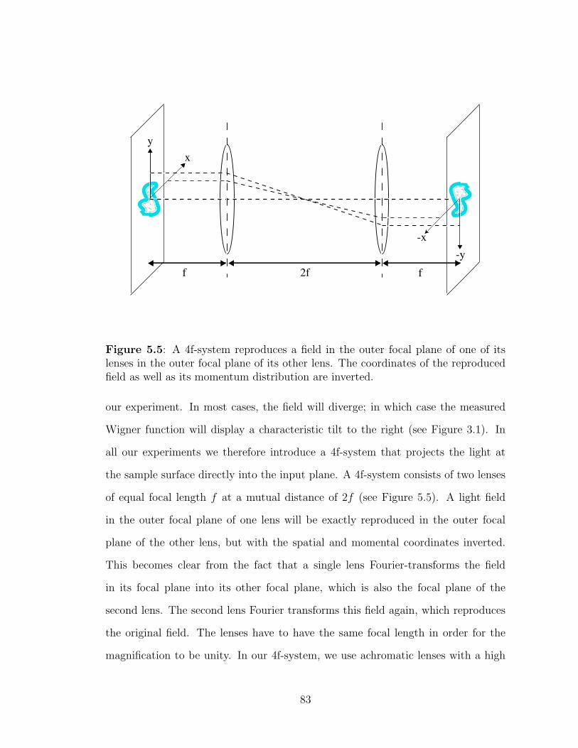
x

-x

y

-y

f f2f

Figure 5.5: A 4f-system reproduces a field in the outer focal plane of one of itslenses in the outer focal plane of its other lens. The coordinates of the reproducedfield as well as its momentum distribution are inverted.

our experiment. In most cases, the field will diverge; in which case the measured

Wigner function will display a characteristic tilt to the right (see Figure 3.1). In

all our experiments we therefore introduce a 4f-system that projects the light at

the sample surface directly into the input plane. A 4f-system consists of two lenses

of equal focal length f at a mutual distance of 2f (see Figure 5.5). A light field

in the outer focal plane of one lens will be exactly reproduced in the outer focal

plane of the other lens, but with the spatial and momental coordinates inverted.

This becomes clear from the fact that a single lens Fourier-transforms the field

in its focal plane into its other focal plane, which is also the focal plane of the

second lens. The second lens Fourier transforms this field again, which reproduces

the original field. The lenses have to have the same focal length in order for the

magnification to be unity. In our 4f-system, we use achromatic lenses with a high

83

numerical aperture. Each lens consists of a convex lens glued to a concave lens made

from a material with higher refractive index. This combination corrects spherical

aberration to a good degree, thereby allowing high-numerical aperture applications

without distortions [47].

In our experiment, the 4f-system is one of the most sensitive parts. Even small

tilts of the lenses with respect to each other, misalignments perpendicular to the

direction of the beam or regarding the mutual distance of the lenses will lead to

distortions in the measured Signal, due to the high phase-sensitivity of the Two-

Window technique.

In all our experiments we use a 4f-system right before the input lens in the

Signal arm in order to project the output field from the sample directly into the

input plane, as can be seen in the following section.

5.8 Overview of complete system

We conclude this chapter with the presentation of the complete experimental setup,

which includes all optical elements which have been omitted for clarity in the pre-

vious sections. Figure 5.6 shows the scheme.

The preparation of a collimated beam from the SLD light is performed by the

optical elements between the SLD and beam splitter BS1. This is discussed in

more detail in Chapter 6. The three lenses and the aperture collimate the beam;

the mirrors M13 and M14 serve to adjust the transverse location and the angle of

the beam entering the system. The λ/2-plate turns the polarization to vertical in

order to avoid polarization effects in the system.

All three AOs are situated in the focal planes of 4f-systems built from lenses

with a focal length of 30 cm (L6-L11). Focusing a beam before sending it through

84

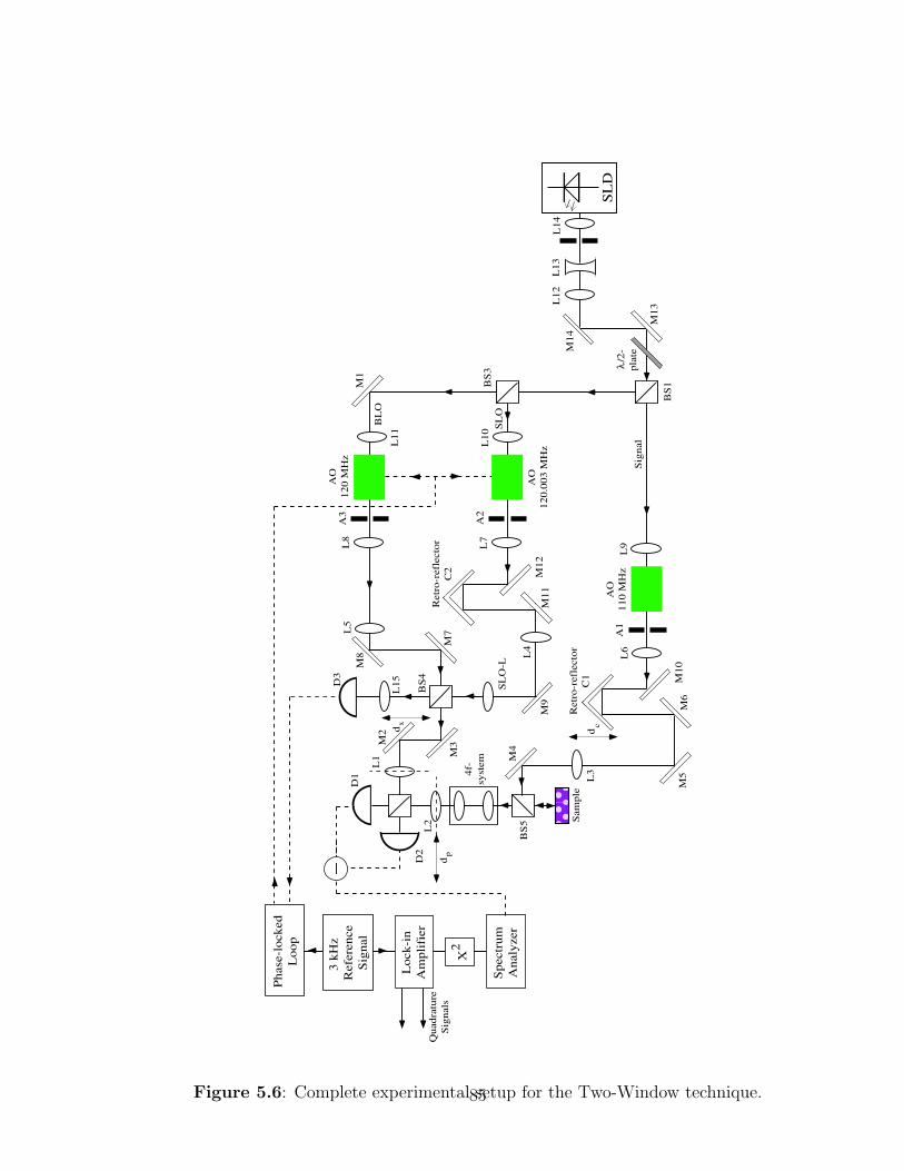
M2

SL

O

Ret

ro-r

efle

ctor

C

1d

c

Sig

nal

AO

12

0.00

3 M

Hz

AO

11

0 M

Hz

M1

BS

1

SL

D

AO

12

0 M

Hz

BS

3

BS

4

SL

O-L

D3

BL

O

X2

Spe

ctru

m

Ana

lyze

r

Loc

k-in

A

mpl

ifie

r

3 kH

z

Ref

eren

ce

Sig

nal

Pha

se-l

ocke

d L

oop

D1

L2

L1

dx

dp

D2

4f-

syst

em

Ret

ro-r

efle

ctor

C

2

L3

L4

L5

L6

L7

L8

L9

L10

L11

M3

M4

M5

M6

M7

M8

M9

M10

M11

M12

M13

M14

L12

L13

L14

A1

A2

A3

L15

Qua

drat

ure

Sig

nals

Sam

ple

BS

5

λ/2

- pl

ate

Figure 5.6: Complete experimental setup for the Two-Window technique.85

an AO crystal is necessary to ensure that the beam hits a region in the AO crystal

where the phase of the acoustic wave is approximately uniform, which guarantees

uniform deflection. A beam diameter on the order of 0.5 mm is recommended by

IsoMET. In order to minimize random differences of the beam profiles of both LOs

and S, the distances between each AO and the initial beam splitter BS1 are set to

be equal.

There are additional lenses with a focal lens of 100 cm in each beam close to

the detector (L3-L5) which allow the fine-tuning of the wavefronts in the input

planes. Transversely partially coherent light has a stronger tendency to diverge

than coherent light. The Two-Window technique is especially sensitive to the radii

of curvature of each beam, which requires a careful alignment of all three correction

lenses.4 A more detailed treatment about the properties of partially coherent light

in this context can be found in Section 6.3.

The Signal beam arm shows the setup for backscatter measurements. The in-

coming Signal beam from M4 is reflected onto the sample by beam splitter B5. The

light backscattered from the sample is projected onto the Signal field input plane at

L2 by the 4f-system. The sample surface is in the first focal plane, the Signal field

input plane in the second focal plane of the 4f-system. The adjustment of the Signal

arm for the measurement of the enhanced backscattering effect will be explained in

detail in Section 12.1.

For transmission experiments, beam splitter BS5 will be replaced by a mirror

and the sample be placed between this mirror and the 4f-system. As before, the

sample surface must be located in the focal plane of the first lens of the 4f-system

(see Section 13.1).

4Even though the SLO has an additional convex lens with a shorter focal lens (SLO− L), thecorrection lens L4 is still useful for initial alignment of the SLO.

86

Chapter 6

The Superluminescent diode

6.1 Introduction

In nearly all of our experiments, a superluminescent light emitting diode SLD by

Superlum Co. serves as a light source. An SLD is an emitter based on stimulated

emission with amplification but insufficient feedback for laser oscillation to build

up [48]. It can be viewed as a semiconductor laser diode with angled cleaved surfaces.

Consequently, the free spectral range is relatively high, resulting in a broad spectra

width on the order of 10 nm. A laser diode on the other hand has typically a spectral

width of just 2-3 nm. Due to the angled structure of the emitter, the emerging light

field is usually non-Gaussian and has an intensity distribution the shape of a sickle.

Its angular spread is on the order of tens of degrees. Therefore the losses for beam-

collimation can be expected to be high; they were measured to be about 70-80%

which coincides with data from Superlum Co. The intricacies of the collimation of

the SLD light and its collimation will be dealt with in Section 6.3.

The SLD is very sensitive to static electricity and other voltage spikes which

might damage its depletion area. Because of its exponential I − V−characteristics,

it requires a current source for operation. Due to the relatively small size of the

emitting area the current density in the emitter can be on the order of tens of

87

kAcm2 . This makes it vulnerable to current spikes and optical feedback which can

lead to local overheating resulting in dopant diffusion or even destruction of the

semiconductor crystal. The power supply and its safety measures regarding the

operation of the SLD will be explained in Section 6.6.

SLDs from Superlum Co. which operate in the visible spectrum use a relatively

new technology which make them very temperature-sensitive. Therefore temper-

ature stabilization is required. A thermistor in combination with a peltier ele-

ment which are mounted in the SLD casing keep the temperature constant down to

milli-Kelvins. A brief description of the temperature stabilization will be given in

Section 6.5

6.2 General parameters of the SLD

In this section we present the intrinsic parameters of the SLD we use as well as the

properties of the collimated beams. The following table shows the most important

parameters of the SLD provided by Superlum Co.:

88

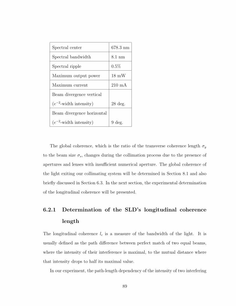
Spectral center 678.3 nm

Spectral bandwidth 8.1 nm

Spectral ripple 0.5%

Maximum output power 18 mW

Maximum current 210 mA

Beam divergence vertical

(e−2-width intensity) 28 deg.

Beam divergence horizontal

(e−2-width intensity) 9 deg.

The global coherence, which is the ratio of the transverse coherence length σg

to the beam size σs, changes during the collimation process due to the presence of

apertures and lenses with insufficient numerical aperture. The global coherence of

the light exiting our collimating system will be determined in Section 8.1 and also

briefly discussed in Section 6.3. In the next section, the experimental determination

of the longitudinal coherence will be presented.

6.2.1 Determination of the SLD’s longitudinal coherence

length

The longitudinal coherence lc is a measure of the bandwidth of the light. It is

usually defined as the path difference between perfect match of two equal beams,

where the intensity of their interference is maximal, to the mutual distance where

that intensity drops to half its maximal value.

In our experiment, the path-length dependency of the intensity of two interfering

89

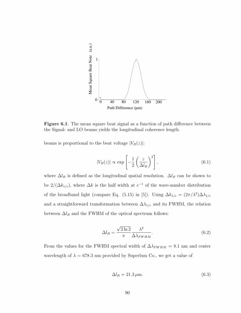
Mea

n Sq

uare

Bea

t Not

e (

a.u.

)

Path Difference (µm)20016012080400

1

0

Figure 6.1: The mean square beat signal as a function of path difference betweenthe Signal- and LO beams yields the longitudinal coherence length.

beams is proportional to the beat voltage |VB(z)|:

|VB(z)| ∝ exp

[−1

2

(z

∆lB

)2]

, (6.1)

where ∆lB is defined as the longitudinal spatial resolution. ∆lB can be shown to

be 2/(∆k1/e), where ∆k is the half width at e−1 of the wave-number distribution

of the broadband light (compare Eq. (5.15) in [5]). Using ∆k1/e = (2π/λ2)∆λ1/e

and a straightforward transformation between ∆λ1/e and its FWHM, the relation

between ∆lB and the FWHM of the optical spectrum follows:

∆lB =

√2 ln 2

π

λ2

∆λFWHM

. (6.2)

From the values for the FWHM spectral width of ∆λFWHM = 8.1 nm and center

wavelength of λ = 678.3 nm provided by Superlum Co., we get a value of

∆lB = 21.3 µm. (6.3)

90

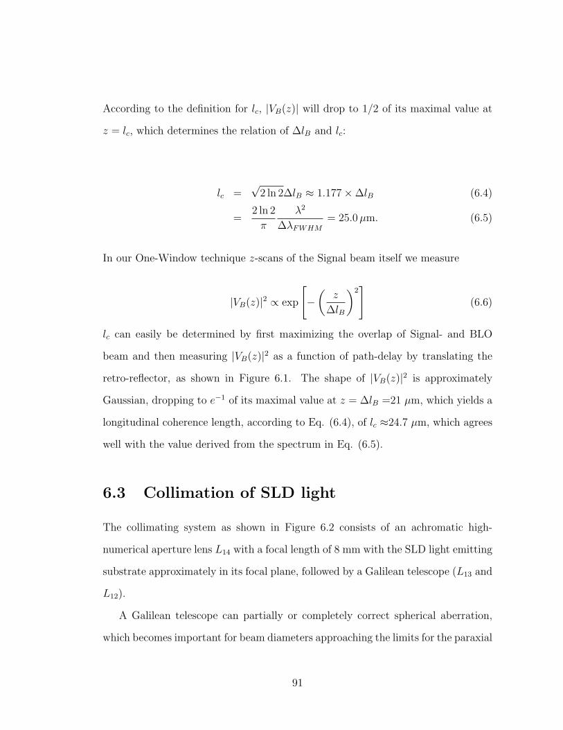
According to the definition for lc, |VB(z)| will drop to 1/2 of its maximal value at

z = lc, which determines the relation of ∆lB and lc:

lc =√

2 ln 2∆lB ≈ 1.177×∆lB (6.4)

=2 ln 2

π

λ2

∆λFWHM

= 25.0 µm. (6.5)

In our One-Window technique z-scans of the Signal beam itself we measure

|VB(z)|2 ∝ exp

[−

(z

∆lB

)2]

(6.6)

lc can easily be determined by first maximizing the overlap of Signal- and BLO

beam and then measuring |VB(z)|2 as a function of path-delay by translating the

retro-reflector, as shown in Figure 6.1. The shape of |VB(z)|2 is approximately

Gaussian, dropping to e−1 of its maximal value at z = ∆lB =21 µm, which yields a

longitudinal coherence length, according to Eq. (6.4), of lc ≈24.7 µm, which agrees

well with the value derived from the spectrum in Eq. (6.5).

6.3 Collimation of SLD light

The collimating system as shown in Figure 6.2 consists of an achromatic high-

numerical aperture lens L14 with a focal length of 8 mm with the SLD light emitting

substrate approximately in its focal plane, followed by a Galilean telescope (L13 and

L12).

A Galilean telescope can partially or completely correct spherical aberration,

which becomes important for beam diameters approaching the limits for the paraxial

91

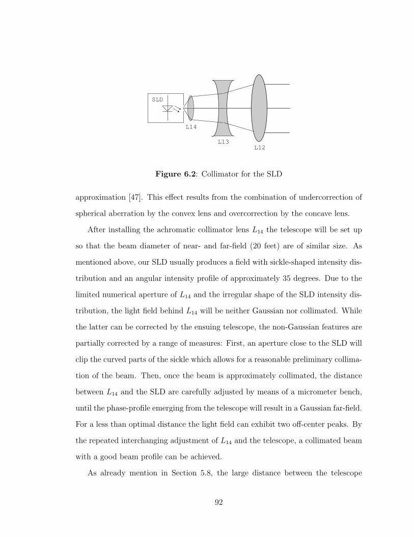
SLD

L14

L13L12

Figure 6.2: Collimator for the SLD

approximation [47]. This effect results from the combination of undercorrection of

spherical aberration by the convex lens and overcorrection by the concave lens.

After installing the achromatic collimator lens L14 the telescope will be set up

so that the beam diameter of near- and far-field (20 feet) are of similar size. As

mentioned above, our SLD usually produces a field with sickle-shaped intensity dis-

tribution and an angular intensity profile of approximately 35 degrees. Due to the

limited numerical aperture of L14 and the irregular shape of the SLD intensity dis-

tribution, the light field behind L14 will be neither Gaussian nor collimated. While

the latter can be corrected by the ensuing telescope, the non-Gaussian features are

partially corrected by a range of measures: First, an aperture close to the SLD will

clip the curved parts of the sickle which allows for a reasonable preliminary collima-

tion of the beam. Then, once the beam is approximately collimated, the distance

between L14 and the SLD are carefully adjusted by means of a micrometer bench,

until the phase-profile emerging from the telescope will result in a Gaussian far-field.

For a less than optimal distance the light field can exhibit two off-center peaks. By

the repeated interchanging adjustment of L14 and the telescope, a collimated beam

with a good beam profile can be achieved.

As already mention in Section 5.8, the large distance between the telescope

92

and the input planes of the detector will lead to a considerable divergence at the

detector for the beam size we use. The additional spread due to the finite transverse

coherence is negligible in our case: With a global coherence σglob = σg/σs of 7.05

(see Section 8.1), the angular spread θs increases by about 4% according to the

relation below [43]:

θs =1√2σsk

√1 +

4

σ2glob

(6.7)

6.4 Drift

The Superlum SLD is based on a relatively new technology which enables the pro-

duction of low-cost, red-light high-power SLDs. One trade-off though is the rela-

tively high sensitivity towards temperature changes and backscattered light.

The SLD casing contains a peltier element and a thermistor which are part of

an electronic temperature stabilization.

During experimental runs I have noticed that the airstream as a result of a

person passing by could already change the direction of the beam considerably. A

cardboard windshield around the SLD an the sealing of the foil curtains around the

optical table with duct tape reduced this kind of drift by 80%.

Even small amounts of light reflecting back into the SLD can lead to changes in

power output and temporal oscillations. In particular, this effect was observed with

light reflecting off an acousto-optic modulator crystal in the signal beam arm. A

brief reflection, e.g. coming from the glass surface of our sample container during

adjustment, usually changes the direction of the output beam for hours.

The remaining drift can not be sufficiently controlled at the moment and presents

a major challenge. Necessary readjustments due to changes in direction as well as

93

the phase- and intensity distribution of the beam generated by the SLD, require

about 99% of the time allocated to experimental work. Drifts over a time period

of minutes to hours necessitate rapid readjustment of all elements involved, and a

comprehensive knowledge of especially drift-sensitive parts of the system which need

frequent readjustments. Furthermore, the ability to quickly interpret and correct

drift-induced aberrations visible in the measured phase-space distribution is imper-

ative: Misalignments of various components in the x− and y−directions display

characteristic distortions in the phase-space diagram. Extremely sensitive measure-

ments, as the ’curvature flipping’-experiment presented in Section 12.2.2, could only

be accomplished by fully exploiting all drift countermeasures. In addition, taking

those scans at night proved beneficial, probably due to less air turbulence and vibra-

tions. With the advancement of SLD technology, these light sources, and especially

those using the novel technology that is employed in our SLD, should hopefully

become more stable.

6.5 Temperature stabilization

The temperature stabilization controller keeps the temperature of the SLD at 25

degrees Celsius in our experiments. This is done by a feedback loop: The controller

measures the temperature of the SLD by means of a temperature-sensitive resistor

and adjusts it by heating or cooling of a thermoelectric cooler (TEC) which holds

the SLD.

The temperature-sensitive resistor is an NTC thermistor (temperature depen-

dent resistor with a negative temperature coefficient) also placed close to the SLD

in its casing.

This thermistor is part of a Wien bridge in the temperature controller, whose

94

voltage output will be adjusted to zero for the value thermistor’s resistance at 25

degrees C. For other temperatures, the Wien bridge will then generate a positive

or negative voltage, depending on whether the measured temperature is higher

or lower than 25 degrees. This voltage is amplified using operational amplifiers

and passed through low-pass filters in order to adjust the time constant of the

temperature control: If the time constant is too fast, the feedback loop and with it

the temperature will oscillate. If the time constant is too slow, it can not keep up

with temperature fluctuations.

The operational amplifiers control a pair of two transistors in push-pull con-

figuration which are connected to the TEC in the SLD casing. The error voltage

generated by the Wien bridge is also used to trigger an alarm to sound in case

the temperature deviates from the selected value by more than a degree. A circuit

diagram of the temperature stabilization is shown in Appendix A.

6.6 SLD power supply

The power supply for the SLD is a stabilized current source. It consists of a MOS-

FET which is controlled by a stabilized, but variable voltage at the gate. The output

circuit contains an internal feedback loop: In the source side of the MOSFET, a

low-ohm resistor is in series with the SLD across which the voltage is measured and

fed back into an OP Amp which controls the MOSFETs gate. This way fluctuations

in the source current can be compensated.

The power supply also has protective measures against current overload as re-

sistors. Diodes in forward and reverse parallel to the SLD shortcut voltage spikes.

In the current setup, the maximum current is limited to 160 mA and the max-

imum voltage to 2.7 V. A circuit diagram of the SLD power supply is shown in

95

Appendix A.

96

Chapter 7

Characterization of a transversebeam profile - Theory

The spatial- and coherence properties of the Signal beam S can easily be determined

using the Two-Window technique: The phase-space profile SB(dx, px) and the lon-

gitudinal profile SB(z) of the Signal beam itself are measured, which then determine

all beam parameters of interest for our experiment. In this chapter we show how to

extract from a transverse scan the beam size σs, the transverse coherence length σg,

and the radius of curvature R of the Signal beam. We use the theory developed here

in the experimental part in Chapter 8. Chapter 9 completes the characterization

of all beams in this experiment with the measurement of the longitudinal coherence

length and the spectral characteristics of our light source. Also in that chapter, a

model for determining the spot-size and Rayleigh length of the small LO (SLO) as

well as a model for mapping the location and frequency-shifts of transverse modes

are introduced.

In the past, we have used the Single-Window technique to characterize the

Signal- and LO-beams. In this technique, the Signal- and the LO-beam are prepared

equally in size and radius of curvature. Then, the phase-space profile of the Signal

beam is measured using the identical LO-beam. This technique requires knowledge

about the preparation of the Signal field to be measured so that the LO can be pre-

97

pared the same. This information is not always available. Also, the Single-Window

technique does not allow for the detection of misalignments below a level that is

necessary for some of the beam parameters to have a reasonable margin of error:

For a radius of curvature of both beams on the order of a meter, a 20% difference of

radius of curvature and beam size in one of the beams, which is difficult to detect

in a convolution of similar beams, can lead to a 50% error in measured beam-size

and 20% error in the transverse coherence length of the beam pair. For a larger

misalignment of more than 25% the measured transverse coherence length goes to-

wards infinity, after that it becomes imaginary. The beam-size on the other hand

goes towards zero.

Using flat wavefronts for the determination of the transverse coherence length

σg has several advantages. Firstly, it is easier to give both the LO- and Signal beam

a nearly flat wavefront than any other finite value which has to be equal for both

beams. Secondly, it turns out that the measured beam parameters then become

much less dependent on differences in beam-size between the beams than for finite

radii of curvature. This is also of importance for the Two-Window technique, where

the big LO (BLO)- and Signal (S) beam are of equal size. Generally, mismatches

in radius of curvature and beam size decrease the measured beam size and increase

the transverse coherence length.

The Two-window uses flat wavefronts for both SLO and BLO, regardless of the

Signal field to be measured.1 In the following sections we show how to determine

two beam parameters while a third is known. For the determination of σs and σg of

the Signal beam as described in Section 7.2, I collimate the Signal beam in order to

make the measurement less dependent on misalignments, as mentioned above. From

1The Single-Window technique could theoretically also be modified so that the preparation ofonly one beam is required, but small misalignments have a larger effect in that case.

98

the measured beam properties we can determine the global coherence σglob = σg/σs

which is the same for all beams. In Section 7.3 I show how to determine σs and

R from a transversely coherent beam, which applies to our system very well, given

the high transverse coherence of the light we employ. In Chapter 8 I use the theory

derived in the current chapter to determine the beam parameters in our experiment.

In Chapter 9 I present the experimental results and a discussion of phase-sensitive

z-scans, i.e., scans which measure the complex beat signal as a function of path-

delay ∆l. We examine the origin and potential applications of a phase-gradient in

the complex beat signal that we observe in these experiments.

7.1 Introduction

7.1.1 Single-Window method

Previously, we have measured the parameters of an identically prepared set of

Signal- and LO beam, using the Single-LO method [2, 3]. In this section, we will

briefly describe the workings of this technique.

From Eq. (4.14) we know the beat voltage for a the superposed Signal- and LO

beams as a function of relative displacement dx and momentum dp to be

VB ∝∫

dη exp

(ik

fηdp

)Γ(η − dx, η)

=

∫dη exp(iηpx) 〈E∗LO(η − dx)ES(η)〉 (7.1)

where 〈...〉 denotes the temporal averaging over the source light. We omitted the

phase-factor exp(−i k2f

d2p) which is identical for SLO and BLO and will cancel when

99

we multiply V SLO∗ and V BLO later on (see Eq. (5.33)). We also abbreviated the

transverse momentum kfdp by px.

The cross-spectral density of the combined field for identical S and LO beam is

given by Eq. (3.2). For two equal-sized beams with a different radius of curvature,

this expression becomes:

Γ(x1, x2) = 〈E∗(x1)E(x2)〉

= exp

(−x2

1 + x22

4σ2s

)exp

[−(x1 ± x2)

2

2σ2g

]exp

(ik

2R1

x21 −

ik

2R2

x22

)

= exp

(− x2

1

4σ2s

+ik

2R1

x21

)exp

(− x2

2

4σ2s

− ik

2R2

x22

)exp

[−(x1 ± x2)

2

2σ2g

]

(7.2)

= 〈E∗(x1)〉〈E∗(x2)〉 exp

[−(x1 ± x2)

2

2σ2g

]. (7.3)

We also replaced the minus in the term containing the transverse coherence length

with a ±. The ± is ”−” when the beam profiles of S and LO match, and ”+”

when they are inverted with respect to each other. Such an inversion only affects

the relative position of the coherence areas, necessitating the change in sign of

one of the spatial variables in the σg-term. In the Single-LO technique, which,

as stated earlier, employs identical beams, x1 − x2 = dx, where dx is again the

perpendicular translation between the beams. If the beam profiles of S and LO are

matched (”−”), the last term in Eq. (7.3) can be simplified accordingly, leading to

the following relation between the cross-spectral density for a partially transversely

coherent beam Γ(x1, x2) and a fully transversely coherent beam 〈E(x1)〉〈E(x2)〉:

Γ(x− dx, x) = exp

(− d2

x

2σ2g

)〈E∗(x− dx)〉〈E∗(x)〉. (7.4)

100

Inserting this expression into Eq. (7.1) yields

V part.coh.B (dx, px) = exp

(− d2

x

2σ2g

) ∫dη exp(iηpx) 〈E∗(x− dx)〉〈E∗(x)〉

= exp

(− d2

x

2σ2g

)V coh

B (dx, px) (7.5)

and consequently

|V incohB (dx, px)|2 = exp

(−d2

x

σ2g

)|V coh

B (dx, px)|2. (7.6)

This demonstrates the simple relationship between the beat voltages of pairs of

equally-sized beams with different transverse coherence: A finite transverse coher-

ence length narrows the position width of the phase-space profile of |VB(dx, px)|2 by

a Gaussian factor. Note that even though the beams have to be equal in size, their

individual radii of curvature can be arbitrary.

Previously, we identically prepared the Signal and the LO beam before deter-

mining their beam parameters. Using relation (7.6) we can readily derive the mean

square beat signal for two arbitrary but equal beams. From Eq. (3.4) we know the

Wigner function of a coherent Gaussian beam to be

W coh(x, p) ∝ exp

[− x2

2σ2s

− 2σ2s(

kx

R+ p)2

]. (7.7)

For transversely coherent light, |VB(dx, px)|2 is just the convolution of the identical

Wigner functions of S and LO, according to Eq. (4.25). This convolution causes a

broadening of |VB(dx, px)|2 in x and p by a factor of√

2 (see Section 5.4.4), resulting

in

101

|V cohB (dx, px)|2 ∝ ∝

∫dx dp WLO(x− dx, p + px) WS(x, p)

= exp

[− x2

4σ2s

− σ2s(

kx

R+ p)2

]. (7.8)

The mean square beat signal for finite transverse coherence length then follows

immediately from Eq. (7.6):

|V part.cohB (dx, px)|2 = exp

[−d2

x

(1

4σ2s

+1

σ2g

)]exp

[−σ2

s

(px + dx

k

R

)2]

(7.9)

which reproduces the result in [3]. In this paper, we measured the position-,

momentum- and position-integrated momentum distribution to determine σs, σg

and R of the equally prepared beam pair.

7.1.2 Two-Window method

In the Two-Window technique we prepare the Dual-LO as usual; the BLO collimated

and the SLO focused. The Signal beam can have an arbitrary Gaussian wavefront.

The fact that no two beams are prepared to be equal leads to a more complex

interplay between the beam parameters. We adapt the expression for the cross-

spectral density in Eq. (7.2) by including beam size scaling factors a, A and B and

different radii of curvature R1, R2 = ∞ for S and LO:

102

Γ(x1, x2) = exp

[−x2

1

(1

4σ2sA

2+

ik

2R1A2

)]exp

[−x2

2

(1

4σ2sB

2− ik

2R2B2

)]

× exp

[−(x1

A± x2

B)2

2σ2g

]. (7.10)

a, A and B are dimensionless scaling parameters which relate the size ratio of a

(potentially modified) beam at the detection input plane to its original size 2σs. For

the BLO and S beam, A and B are usually close to 1, while for the SLO a is on the

order of 0.1. Note that the definition of a, A and B is different than in Section 5.3,

where they denoted the respective beam-sizes itself.

In the following sections, we will calculate the complex beat signal for the two

most important cases: a flat Signal beam of finite transverse coherence length (Sec-

tion 7.2) and a transversely coherent beam with a finite radius of curvature (Sec-

tion 7.3). For both cases, we will show how to extract the remaining unknown

parameters.

7.2 R=∞, σs and σg unknown

In this section, we will show how to determine σs and σg of a flat Signal beam of

arbitrary transverse coherence. We first derive the general expression for the beat

voltage between the Signal beam and an LO (Section 7.2.1), followed by the beat

voltage for a close-to perfect SLO (Section 7.2.2) and a BLO about the size of the

Signal beam (Section 7.2.3) as used in our experiment. From the complex beat

signal calculated in Section 7.2.4 we show how to extract σs and σg from either

quadrature signal (Section 7.2.5).

103

7.2.1 General beat voltage

Inserting Eq. (7.10) into Eq. (7.1) and setting R1 = ∞ (flat LO) and R2 = ∞ (flat

Signal beam), we get for the beat voltage of the S and BLO beams:

VB(dx, px) ∝∫

dη exp(iηpx)

× exp

− 1

4σ2s

[(η − dx)

2

A2+

η2

B2

]− 1

2σ2g

(η − dx

A± η

B

)2

= exp

−dx2

[1

A2

(1

4σ2s

+1

2σg

)]

×∫

dη exp

−η2

[1

4σ2s

(1

A2+

1

B2

)+

1

2σ2g

(1

A2+

1

B2± 2

AB

)]

+ 2η

[ipx

2+

dx

2σ2g

(1

A2± 1

AB

)]. (7.11)

By defining ρ = 14σ2

s+ 1

2σ2g

we get

VB(dx, px) ∝ exp(−d2x

ρ

A2)

×∫

dη exp

−η2

[ρ

(1

A2+

1

B2

)± 1

σ2gAB

]

+ 2η

[ipx

2+ dx

(ρ2

A2± 1

2σ2gAB

)]

∝ exp(−d2x

ρ

A2) exp

[ipx

2+ dx(

ρA2 ± 1

2σ2gAB

)]2

ρ( 1A2 + 1

B2 )± 1σ2

gAB

= exp(−d2x

ρ

A2)

× exp

1

ρ( 1A2 + 1

B2 )± 1σ2

gAB

[−d2

x

(ρ

A2± 1

2σ2gAB

)2

− p2x

4+ idxpx

(ρ

A2± 1

2σ2gAB

)].

(7.12)

104

While the pre-factors for px and dxpx can not be simplified any further, the prefactor

dx can be transformed as follows:

−prefdx =ρ

A2+

( ρA2 ± 1

2σ2gAB

)2

( 1A2 + 1

B2 )± 1σ2

gAB

=ρ

A2−

ρ2

A4 ± ρA2

1σ2

gAB+ 1

4σ4A2B2

ρA2 + ρ

B2 ± 1σ2

gAB

=ρ

A2− ρ

A2

ρA2 ± 1

σ2gAB

+ 14ρσ4B2

ρA2 + ρ

B2 ± 1σ2

gAB

. (7.13)

For simplicity we define ξ = ρA2 ± 1

σ2AB:

−prefdx =ρ

A2− ρ

A2

ξ + 14ρσ4B2

ξ + ρB2

=ρ

A2

[1−

ξ + 14ρσ4

gB2

ξ + ρB2

]

=ρ

A2

[ξ + ρ

B2 − ξ − 14ρσ4

gB2

ξ + ρB2

]

=ρ

A2

[ ρB2 − 1

B2(σ4g/σ2

s+2σ2g)

ρ( 1A2 + 1

B2 )± 1σ2

gAB

]

=ρ

A2B2

ρ− σ2s/σ2

g

σ2g+2σ2

s

( 1A2 + 1

B2 )[ρ± 1σ2

g(BA

+ AB

)]

. (7.14)

The numerator can be simplified even further:

105

ρ

(ρ− σ2

s/σ2g

σ2g + 2σ2

s

)

=

(1

4σ2s

+1

2σ2g

)(1

4σ2s

+1

2σ2g

− σ2s/σ

2g

σ2g + 2σ2

s

)

=

(1

4σ2s

+1

2σ2g

)2[1− σ2

s/σ2g

( 14σ2

s+ 1

2σ2g)(σ2

g + 2σ2s)

]

=

(1

4σ2s

+1

2σ2g

)21− 1

σ4g

4σ4s

+σ2

g

σ2s

+ 1

=

(1

4σ2s

+1

2σ2g

)21− 1

(σ2

g

2σ2s

+ 1)2

=

(1

4σ2s

+1

2σ2g

)2[1− 1

4σ4( 14σ2

s+ 1

2σ2g)2

]

=

(1

4σ2s

+1

2σ2g

)2

− 1

σ4g

= ρ2 − 1

4σ4g

=

(ρ− 1

2σ2g

)(ρ +

1

2σ2g

). (7.15)

Inserting this expression into Eq. (7.14) and also simplifying the first two terms in

the denominator of Eq. (7.14) finally yields:

prefdx =1

A2 + B2

(ρ− 12σ2

g)(ρ + 1

2σ2g)

ρ± 1σ2

g(BA

+ AB

)

. (7.16)

The complete expression for VB(dx, dp) then becomes:

106

VB(dx, px) ∝ exp

−d2

x

1

A2 + B2

(ρ− 12σ2

g)(ρ + 1

2σ2g)

ρ± 1σ2

g(BA

+ AB

)

− p2x

1

4[ρ( 1A2 + 1

B2 )± 1σ2

gAB]

+ idxpx

ρ/A2 ± 12σ2

gAB

ρ( 1A2 + 1

B2 )± 1σ2

gAB

(7.17)

Using this general expression we now calculate the VB(dx, dp) for our SLO (A ¿ B)

and the special BLO we use (A = B).

7.2.2 Beat voltage for a close-to perfect SLO (A ¿ B)

For a close-to perfect SLO, i.e., A ¿ B, the expression in Eq. (7.17) simplifies

considerably:

V SLOB (dx, px) ∝ exp

− d2

x

B2

ρ2 − 14σ4

g

ρ− p2

x

4[ρ/A2]+ idxpx

ρA± 1

2σ2gB

ρA± 1

σ2gB

= exp

−

d2x

B2

ρ− 1

σ4g

σ2s

+ 2σ2g

− p2

x

A2

4ρ+ ipxdx

. (7.18)

The prefactor for p2x goes towards zero as expected for an SLO, which has a big

momentum spread. The prefactor for dx simplifies as shown below:

107

prefdx =1

4σ2s

+1

2σ2g

− 1σ4

g

σ2s

+ 2σ2g

=1

4σ2s

+1

2σ2g

1− 2σ2

g

σ4g

σ2s

+ 2σ2g

=1

4σ2s

+1

2σ2g

1− 1

σ2g

2σ2s

+ 1

=1

4σ2s

+1

2σ2g

1

1 + 2σ2s

σ2g

=1

4σ2s

+1

2σ2g + 4σ2

s

. (7.19)

Inserting Eq. (7.19) into Eq. (7.18) yields the final expression for the beat voltage

for the SLO:


[− d2

x

B2

(1

4σ2s

+1

2σ2g + 4σ2

s

)+ idxpx

](7.20)

which is independent of a potential inversion between SLO and S.

7.2.3 Beat voltage for our special BLO (A = B)

For a BLO the same size as the Signal beam (A = B), Eq. (7.17) simplifies as well:

V BLOB (dx, px) ∝ exp

[− d2

x

2B2

(ρ− 12σ2

g)(ρ + 1

2σ2g)

ρ± 12σ2

g

− p2x

4B2 (

12σ2

s+ 1

σ2g± 1

σ2g)

+ idxpx

1B2 (

14σ2 + 1

2σ2g± 1

2σ2g)

1B2 (

12σ2

s+ 1

σ2g± 1

σ2g)

]. (7.21)

108

Depending on the sign which signifies an inversion between BLO and S, we get two

different results. If the beam profiles are matched, we get

VBLO(−)B (dx, px) ∝ exp

[− d2

x

2B2

(ρ +

1

2σ2g

)− p2

xB2

4( 12σ2

s)

+ idxpx

14σ2

s

12σ2

g

]

= exp

[− d2

x

B2

(1

8σ2s

+1

2σ2g

)− p2

x

B2σ2s

2+ i

dxpx

2

]. (7.22)

In case BLO is inverted with respect to S, expression (7.21) becomes:

VBLO(+)B (dx, px)

∝ exp

[− d2

x

2B2

(ρ− 1

2σ2g

)− p2

xB2

4

1

2σ2s+ 2

σ2g

+ idxpx

1B2

1

4σ2s+ 1

σ2g

1

B2

1

2σ2s+ 2

σ2g

]

= exp

[− d2

x

8B2σ2s− p2

xB2

2

σ2s+ 8

σ2g

+ idxpx

2

]. (7.23)

Notice that for matched beam profiles the position distribution depends on 18σ2

s+ 1

2σ2g,

while the momentum distribution only on σ2s . For inverted beam profiles, it is

exactly the other way around.

7.2.4 Complex beat signal SB(dx, px)

Now that we know the beat voltages for both SLO and BLO, we can calculate the

complex beat voltage which - as stated in Section 5.4.1 - consists of the cross terms

from |V SLOB + V BLO

B |2 as seen in Eq. (5.33):

SB(dx, dp) ∝ V SLO∗B V BLO

B (7.24)

109

where we omitted the frequency-dependent factor. The resulting complex beat

signals for non-inverted (−) and inverted (+) Dual-LO are:

S(−)B (dx, px) ∝ exp

[−d2

x

(3

8σ2s

+1

2σ2g

+1

4σ2s + 2σ2

g

)− p2

x

σ2s

2− i

dxpx

2

](7.25)

S(+)B (dx, px) ∝ exp

−d2

x

(3

8σ2s

+1

4σ2s + 2σ2

g

)− p2

x

1

2(

1σ2

s+ 4

σ2g

) − idxpx

2

.

(7.26)

Figure 5.3 in Section 5.4.2 shows a numerical simulation of the in-phase and out-

of-phase quadrature signals, which are the real and imaginary part of the complex

beat signal, of a collimated partially coherent Gaussian beam for typical values of

σs and σg, according to Eq. (7.25) or Eq. (7.26).

7.2.5 Extraction of σs and σg from the quadrature signals

From the complex beat signal SB(dx, px) measured in our experiment, the coeffi-

cients of dx and px in Equations (7.25) and (7.26) can be determined. We can then

solve for the beam size σs and the transverse coherence length σg. In the following,

we will abbreviate the coefficients as follows:

(dex)

2 =

(3

8σ2s

+1

2σ2g

+1

4σ2s + 2σ2

g

)−1

(7.27)

(pex)

2 =2

σ2s

(7.28)

for the non-inverted Dual-LO, and

110

(dex)

2 =

(3

8σ2s

+1

4σ2s + 2σ2

g

)−1

(7.29)

(pex)

2 = 2

(1

σ2s

+4

σ2g

)(7.30)

for the inverted Dual-LO, so that

SB(dx, px) ∝ exp

[− d2

x

(dex)

2− p2

x

(pex)

2− i

dxpx

2

]. (7.31)

Both the in-phase- and out-of-phase quadrature signal contain all information about

σs and σg. When we use the in-phase signal, we measure the e−1-width of its x-

and p− distribution individually holding its respective conjugate coordinate at zero.

In this case the term containing the variable held at zero as well as the phase in

Eq. (7.31) cancels.2 For example, if we set dx ≡ 0, the d2x and dxpx terms cancel.

SB(dx ≡ 0, px) is then maximal at px = 0 and drops to e−1 of that value at a

momentum pex which can be measured. The extraction of de

x works similarly, when

we set px ≡ 0.

The out-of-phase signal also contains the beam parameters for example in the

distance of its four peaks from another (see Figure 5.3). In the following we will

derive how σs and σg determine the location of those peaks.

The out-of-phase signal, which is the imaginary part of the complex beat signal

(see Eq. (5.16)), is of the form

f(x, p) = exp(−ax2 − bp2) sinxp

2(7.32)

2One has to keep in mind that this is only true when R = ∞ for all beams, as is the case here.For finite radii, SB contains additional phase factors which shift the phase of both quadraturesignals. This will be subject of Section 7.3.

111

where x = dx, p = px and

a =1

(dex)

2(7.33)

b =1

(pex)

2. (7.34)

At the location (xm, pm) of the extrema, the derivatives of f(x, p) with respect to

both variables must be zero:

df(x, p)

dx

∣∣∣∣xm,pm

=[pm

2cos

(xmpm

2

)− 2axm sin

(xmpm

2

)]exp(−ax2

m − bp2m)

= 0 (7.35)

df(x, p)

dp

∣∣∣∣xm,pm

=[xm

2cos

(xmpm

2

)− 2bpm sin

(xmpm

2

)]exp(−ax2

m − bp2m)

= 0 (7.36)

which requires the terms in squared brackets to vanish. Regrouping its terms yields:

pm

4axm

= tan(xmpm

2

)(7.37)

xm

4bpm

= tan(xmpm

2

). (7.38)

Solving for a and b and replacing them with 1(de

x)2and 1

(pex)2

then leads to the final

expressions

112

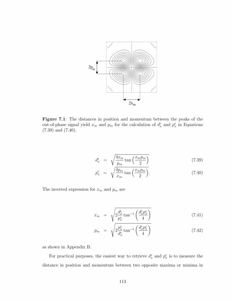
2pm

2xm

Figure 7.1: The distances in position and momentum between the peaks of theout-of-phase signal yield xm and pm for the calculation of de

x and pex in Equations

(7.39) and (7.40).

dex =

√4xm

pm

tan(xmpm

2

)(7.39)

pex =

√4pm

xm

tan(xmpm

2

). (7.40)

The inverted expression for xm and pm are

xm =

√2de

x

pex

tan−1

(de

xpex

4

)(7.41)

pm =

√2pe

x

dex

tan−1

(de

xpex

4

)(7.42)

as shown in Appendix B.

For practical purposes, the easiest way to retrieve dex and pe

x is to measure the

distance in position and momentum between two opposite maxima or minima in

113

the out-of-phase phase-space diagram, as shown in Figure 7.1, divide by 2 to get

xm and pm and calculate dex and pe

x using the expressions (7.39) and (7.40). From

there we solve for σs and σg as shown below.

The advantage of using the out-of-phase signal to extract the beam parameters

is that the procedure only requires measuring a distance as opposed to fitting a

Gaussian to a curve to measure its width as in the case for the in-phase part.

Now that we know dex and pe

x, either from the measured in-phase or out-of-phase

quadrature signal for the Signal beam, we need to calculate an expression for σs and

σg in terms of those parameters, in order to extract them from the measurements.

Let us first consider the case for non-inverted S and Dual-LO, expressed in Eq.

(7.25). We have:

[pex]

2 =2

[σ(−)s ]2

(7.43)

Solving for σs yields

σ(−)meass =

√2

pex

. (7.44)

We added meas to the superscript to emphasize that σs was determined from the

measured value of pex.

Again, according to Eq. (7.25), we have for [dex]

2:

[dex]

2 =

[3

8[σmeas(−)s ]2

+1

2σ2g

+1

4[σmeas(−)s ]2 + 2σ2

g

]−2

(7.45)

We already know σmeas(−)s so we solve for σ

meas(−)g :

114

σmeas(−)g = σs

√7− 8σ2

s/[dex]

2 ±√

25− 48σ2s/[d

ex]

2 + 64σ4s/[d

ex]

4

−3 + 8σ2s/[d

ex]

2(7.46)

where we omitted the superscript meas(-) of σs for the sake of visual clarity. The

procedure for extracting σmeas(+)s and σ

meas(+)g is similar. Equations (7.47) and

(7.48) show the results:

σmeas(+)s =

√√√√−8/[de

x]2 − 5

2[pe

x]2 ±

√64/[de

x]4 − 24[pe

x]2/[de

x]2 + 25

4[pe

x]4

8[pex]/[d

ex]

(7.47)

σmeas(+)g =

√√√√8/[dex]

2 − 72[pe

x]2 ±

√64/[de

x]4 − 24[pe

x]2/[de

x]2 + 25

4[pe

x]4

4[pex]

2/[dex]

2 − 34[pe

x]4

.

(7.48)

There are obviously two sets of solutions for both parameters σs and σg, but only

one set where both parameters are real. From σmeas(±)s and σ

meas(±)g the global

coherence

σmeas(±)glob =

σmeas(±)g

σmeas(±)s

. (7.49)

can be calculated, which does not change during propagation through free space or

first-order optical systems as lenses [43]. We will apply this theory to the determi-

nation of σs and σg of a flat Gaussian Signal beam in Section 8.1.

115

7.3 σg=∞, σs and R unknown

In this section we will show how to extract the beam size σs and the radius of

curvature R from a transversely coherent Signal beam. We again assume the SLO

to be close to perfect. For the BLO, we consider two frequently encountered cases

in our experiment; where the BLO is close to the size of the Signal beam (A = B),

and where it is much larger.

First, we will derive the beat voltage for a LO of arbitrary size in Section 7.3.1.

We use this result to derive the beat voltages for a perfect SLO (Section 7.3.2), a

BLO the size of the Signal beam (Section 7.3.3) and an ideal BLO (Section 7.3.4).

Using these results, we calculate the complex beat signal (Section 7.3.5) and an

approximation of the complex beat signal for small R which we frequently use

(Section 7.3.6). We conclude this theory chapter by showing how to extract σs and

R from the measured complex beat signal (Section 7.3.7).

7.3.1 General beat voltage

Inserting Eq. (7.10) into Eq. (7.1) again we can write the beat voltage of the Signal-

with a general LO beam for this case (σg →∞, R2 = RLO →∞) as

VB(dx, px) =

∫dx exp(ixp) exp

[−(x− dx)

2

4σ2sA

2− x

4σ2sB

2− i

k

2R

x2

B2

]. (7.50)

Solving the integral yields

VB(dx, px) ∝ exp

(− d2

x

4σ2sA

2

)exp

[( dx

4σ2sA2 + ipx

2)2

14σ2

sA2 + 14σ2

sB2 + i k2RB2

]. (7.51)

116

Transformation of the denominator results in

11

4σ2sA2 + 1

4σ2sB2 + i k

2RB2

= 4σ2sA

2 1 + A2

B2 − i2σ2s

A2

B2kR

(1 + A2

B2 )2 + 4σ4s

A4

B4 (kR)2

. (7.52)

Combining Equations (7.51) and (7.52) yields

VB(dx, px) ∝ exp

(− d2

x

4σ2sA

2

)

× exp

[(d2

x

4σ2sA

2− p2

xσ2sA

2 + ipxdx

)1 + A2

B2 − i2σ2s

A2

B2kR

(1 + A2

B2 )2 + 4σ4s

A4

B4 (kR)2

].

(7.53)

Let us abbreviate the size ratio of BLO and S as well as the denominator in the

second exponential as follows:

g ≡ A

B(7.54)

m(g, R) ≡ (1 + g2)2 + 4σ4sg

4(k

R)2. (7.55)

Regrouping the terms according to the order of dx and px, we can then rewrite Eq.

(7.53) as

117

VB(dx, px) ∝ exp

− d2

x

4σ2sA

2

[1− 1 + g2

m(g,R)− i

k

2RB2

1

m(g, R)

]

× − p2x

m(g, R)

[σ2

sA2(1 + g2) + i2σ4

sg4 k

R

]

× pxdx

m(g, R)

[2σ2

sg2 k

R+ i(1 + g2)

]. (7.56)

Using this general expression we can calculate the beat voltages for three types of

LOs: g ¿ 1 (SLO), g = 1 (our BLO which is the size of the Signal beam) and

g → ∞ (ideal BLO). g = 1 does not necessarily represent the case of identical LO

and S as in Section 7.2, where we used a collimated Signal beam: the preparation of

a divergent or convergent Signal beam by means of a lens changes the beam width

in the detection input plane, provided there is a non-zero distance between lens and

input-plane.

7.3.2 Beat voltage for a perfect SLO (A ¿ B)

For g ¿ 1, all terms except for the d2x-terms and the ipxdx-term are negligible. The

beat signal for the SLO is then:


− d2

x

4σ2sA

2

[1− 1 + g2

(1 + g2)2 + 4σ4sg

4( kR)2

]− i

d2x

B2

k

2R+ ipxdx

.

(7.57)

The real pre-factor of −d2x simplifies as shown below:

118

1

4σ2sA

2

[1− 1 + g2

(1 + g2)2 + 4σ4sg

4( kR)2

]

≈ 1

4σ2sA

2

[1− 1 + A2

B2

(1 + A2

B2 )2

]≈ 1

4σ2sA

2

(1− 1 + A2

B2

1 + 2A2

B2

)

=1

4σ2sA

2

A2

B2

1 + 2A2

B2

≈ 1

4σ2sB

2. (7.58)

The complete expression for V SLOB is thus


(− d2

x

4σ2sB

2− i

d2x

2B2

k

R+ ipxdx

). (7.59)

V SLOB (dx, px) is therefore directly proportional to the amplitude and phase of the

curved Signal field, given by the first two terms in Eq. (7.59). The third term is

just due to the fact that we change the relative momentum px between S and SLO

in the Signal arm rather than the LO-arm: If we replace the x in exp(ixpx) in Eq.

(7.50) by x − dx, which would correspond to tilting the respective LO rather than

S, this phase-factor cancels, but will then turn up in the BLO beat signal.

7.3.3 Beat voltage for our special BLO (A = B)

For g = 1,

m(g, R) → 4 + 4σ4(k

R)2. (7.60)

Eq. (7.56) then simplifies to:

119

V g=1B (dx, px) ∝

exp

−d2

x

[1

4σ2sB

2

(1− 2

4 + 4σ4s(

kR)2

)− i

1

B2

k2R

4 + 4σ4s(

kR)2

]

−p2x

[σ2

sB2 2

4 + 4σ4s(

kR)2

+ iB2 2σ4s

kR

4 + 4σ4s(

kR)2

]

+2pxdx

[σ2

skR

4 + 4σ4s(

kR)2

+ i2

4 + 4σ4s(

kR)2

]. (7.61)

The real exponentials can be simplified even further:

− d2x

4σ2sB

2

[2 + 4σ4

s(kR)2

4 + 4σ4s(

kR)2

]− p2

x

[σ2

sB2 2

4 + 4σ4s(

kR)2

]+ 2pxdx

[σ2

skR

4 + 4σ4s(

kR)2

]

= − d2x

4σ2sB

2

[2 + 2σ4

s(kR)2

4 + 4σ4s(

kR)2

]

− d2x

σ2s(

kR)2

2B2[4 + 4σ4s(

kR)2]− p2

x

[σ2

sB2 2

4 + 4σ4s(

kR)2

]+ 2pxdx

[σ2

skR

4 + 4σ4s(

kR)2

]

= − d2x

8σ2sB

2−

(dxkR

σs√2B− pxσs

√2B)2

4 + 4σ4s(

kR)2

. (7.62)

The final expression for V g=1B then reads:

V g=1B (dx, px) ∝ exp

[− d2

x

8σ2sB

2−

(dxkR

σs√2B− pxσs

√2B)2

4 + 4σ4s(

kR)2

]

× exp

[i

4 + 4σ4s(

kR)2

(−d2

x

k

2B2R+ 2B2p2

xσ4s

k

R+ 2dxpx

)].

(7.63)

120

7.3.4 Beat voltage for a perfect BLO (A À B)

For g →∞, i.e., for a perfect BLO,

m(g, R) → g4

[1 + 4σ4

s(k

R)2

]. (7.64)

All pre-factors in Eq. (7.56), except for those of p2x, vanish. We get

V g→∞B ∝ exp

−p2

xσ2s

[A2(1 + A2

B2 )A4

B4 [1 + 4σ4s(

kR)2]− i

2σ2s

kR

A4

B2

A4

B4 [1 + 4σ4s(

kR)2]

]

= exp

−p2

xσ2s

[A4

B2

A4

B4 [1 + 4σ4s(

kR)2]− i2B2 σ2

skR

1 + 4σ4s(

kR)2

]

= exp

−p2

xσ2sB

2

[1

1 + 4σ4s(

kR)2− i2

σ2s

kR

1 + 4σ4s(

kR)2

]. (7.65)

7.3.5 Complex beat signal SB(dx, px)

Using the beat voltages calculated in the previous sections (Section 7.3.2-Section 7.3.4),

we can calculate the complex beat signal we expect. In all of our experiments involv-

ing the characterization of the divergent or convergent Signal beam itself, the BLO

generally has a larger diameter than the Signal beam, so that we can approximate

the BLO to a very good degree to be perfect, i.e. infinitely wide. The remaining

scaling factor B then becomes meaningless and we can set it to unity.

Using the results for V g¿1B (Eq. (7.59)) and V g→∞

B (Eq. (7.69)) to describe the

beat voltages for SLO and BLO, we get for the complex beat signal:

121

SB(dx, px) ∝ V SLO∗B (dx, px)V

BLOB (dx, px)

∝ exp

[− d2

x

4σ2s

− p2x

σ2s

1 + 4σ4s(

kR)2

]

× exp

i

[d2

x

2

k

R+ 2σ2

sp2x

σ2s

kR

1 + 4σ4s(

kR)2− pxdx

]. (7.66)

It can readily be seen that, unlike Single-LO beat signals, for curved Signal beams

(see Eq. (7.9)), there is no correlation between position and momentum in the

magnitude of the beat signal. All information on the radius of curvature is contained

in the phase of SB(dx, px).3

7.3.6 Approximation of SB(dx, px) for small R

If, for a given σs and k, the radius of curvature of the Signal beam is sufficiently

small, Eq. (7.66) can be simplified even further. Let us assume the phase-difference

between the center of the beam and the transverse position 2σs where the relative

field amplitude drops to e−1, is large compared to unity, i.e.

k

2|R|(2σs)2 À 1, (7.67)

where R can be positive or negative. Squaring both sides yields

4σ4s

k2

R2À 1 (7.68)

3For a less than ideal Dual-LO on the other hand, there is a correlation between position andmomentum in the amplitude due to the finite and non-zero size and angular spread of the LOs.

122

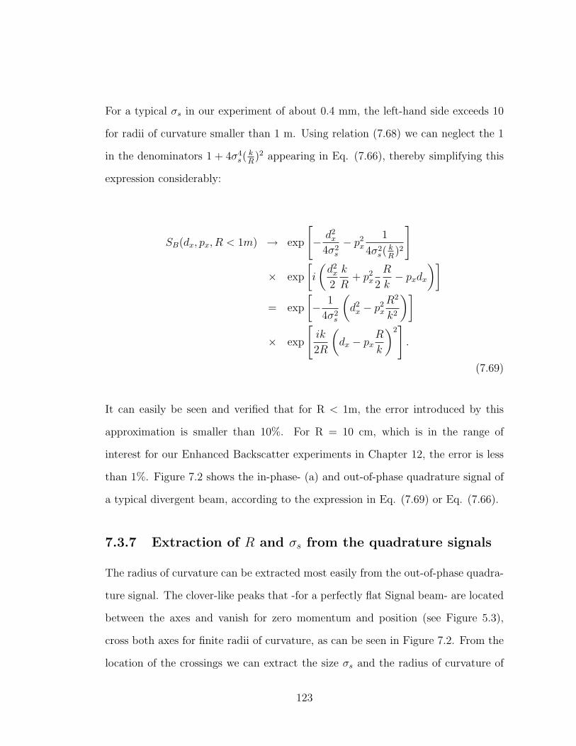
For a typical σs in our experiment of about 0.4 mm, the left-hand side exceeds 10

for radii of curvature smaller than 1 m. Using relation (7.68) we can neglect the 1

in the denominators 1 + 4σ4s(

kR)2 appearing in Eq. (7.66), thereby simplifying this

expression considerably:

SB(dx, px, R < 1m) → exp

[− d2

x

4σ2s

− p2x

1

4σ2s(

kR)2

]

× exp

[i

(d2

x

2

k

R+ p2

x 2

R

k− pxdx

)]

= exp

[− 1

4σ2s

(d2

x − p2x

R2

k2

)]

× exp

[ik

2R

(dx − px

R

k

)2]

.

(7.69)

It can easily be seen and verified that for R < 1m, the error introduced by this

approximation is smaller than 10%. For R = 10 cm, which is in the range of

interest for our Enhanced Backscatter experiments in Chapter 12, the error is less

than 1%. Figure 7.2 shows the in-phase- (a) and out-of-phase quadrature signal of

a typical divergent beam, according to the expression in Eq. (7.69) or Eq. (7.66).

7.3.7 Extraction of R and σs from the quadrature signals

The radius of curvature can be extracted most easily from the out-of-phase quadra-

ture signal. The clover-like peaks that -for a perfectly flat Signal beam- are located

between the axes and vanish for zero momentum and position (see Figure 5.3),

cross both axes for finite radii of curvature, as can be seen in Figure 7.2. From the

location of the crossings we can extract the size σs and the radius of curvature of

123

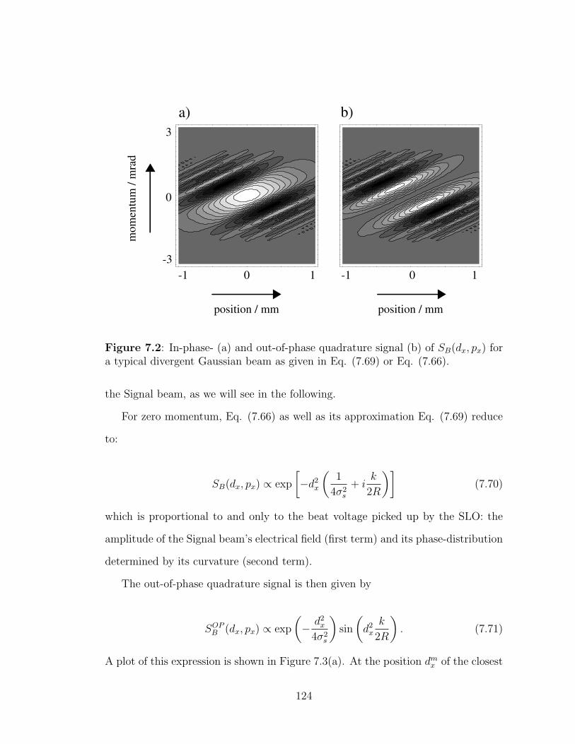
0 0

0

1 1 -1 -1

3

-3

position / mm position / mm

mom

entu

m /

mra

d

a) b)

Figure 7.2: In-phase- (a) and out-of-phase quadrature signal (b) of SB(dx, px) fora typical divergent Gaussian beam as given in Eq. (7.69) or Eq. (7.66).

the Signal beam, as we will see in the following.

For zero momentum, Eq. (7.66) as well as its approximation Eq. (7.69) reduce

to:

SB(dx, px) ∝ exp

[−d2

x

(1

4σ2s

+ ik

2R

)](7.70)

which is proportional to and only to the beat voltage picked up by the SLO: the

amplitude of the Signal beam’s electrical field (first term) and its phase-distribution

determined by its curvature (second term).

The out-of-phase quadrature signal is then given by

SOPB (dx, px) ∝ exp

(− d2

x

4σ2s

)sin

(d2

x

k

2R

). (7.71)

A plot of this expression is shown in Figure 7.3(a). At the position dmx of the closest

124

position / mm

0

1-1

a) b)

3-3

momentum / mrad

S (d , p = 0)OPB x x S (d = 0, p )OP

B x x

-dxm dx

m -pxm px

m

Figure 7.3: The position distribution for zero momentum (a) and the momentumdistribution at the beam center (b) of the out-of-phase quadrature part of SB(dx, px)are used to extract σs and R.

peaks, which correspond to the intersection of the clover peaks in phase-space with

the dx-axis, the derivative of SOPB (dx, px) with respect to dx must vanish:

dSOPB (dx, 0)

d(dx)

∣∣∣∣dm

x

= 0

=

− dm

x

2σ2s

sin

[(dm

x )2 k

2R

]+ dm

x

k

Rcos

[(dm

x )2 k

2R

]

× exp

[−(dm

x )2

4σ2s

](7.72)

which requires the term in the braces to vanish. Rearranging and solving for σs

yields

σs =

√R

2ktan

[(dm

x )2k

2R

]. (7.73)

The next step is to find the crossings of the clover peaks with the p-axis (Fig-

ure 7.3(b)). We use the approximate expression in Eq. (7.69) here since in our

125

experiment we are exclusively concerned with radii of curvature ¿ 1 m, and we can

express R and σs in a closed form. If we used the full expression in Eq. (7.66) we

would have to rely on iterative numerical methods.

For x ≡ 0, Eq. (7.69) reduces to

SB(dx, px) ∝ exp

[−p2

x

(1

4σ2s

R2

k2− i

R

2k

)](7.74)

with the out-of-phase part being

SOPB (dx, px) ∝ − exp

[−p2

x

(R

2σsk

)2]

sin

(p2

x

R

2k

). (7.75)

Again, the derivative of SOPB (dx, px), this time with respect to px, has to be zero at

the intersection pmx between the clover peaks and the p-axis:

dSOPB (0, px)

d(px)

∣∣∣∣pm

x

= 0

= −

pxR

kcos

[(pm

x )2 R

2k

]− (pm

x )

2

(R

σsk

)2

sin

[(pm

x )2 R

2k

]

× exp

[−(pm

x )2

(R

2σsk

)2]

. (7.76)

As before, the term in braces has to be zero in order for the equation to hold.

Rearranging and solving for σs yields

σs =

√R

2ktan

[(pm

x )21

2

R

k

]. (7.77)

By comparing Eq. (7.77) to Eq. (7.73) it is clear that the arguments of their

respective tangent have to be equal, resulting in an expression for R:

126

(pmx )2 R

2k= (dm

x )2 k

2R(7.78)

R = ±dmx

pmx

k. (7.79)

The ”+” holds if the phase-space profile is tilted in the direction where dx and px

have the same sign, and ”−” for different signs; which is the reasoning outlined in

Section 3.4. The above expression is identical to the one we use to determine R from

the plot of Wigner function itself, when we consider pmx

dmx

its slope in phase-space.

We use the R extracted in Eq. (7.79) to determine σs in either Eq. (7.77) or

Eq. (7.73):

σs =

√12

dmx

pmx

tan(

dmx pm

x

2

). (7.80)

We will apply this theory to the determination of R and σs for a divergent Gaussian

Signal beam in Section 8.2.

127

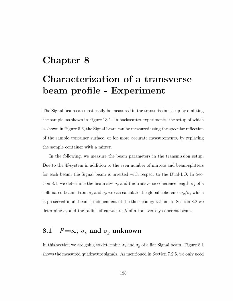
Chapter 8

Characterization of a transversebeam profile - Experiment

The Signal beam can most easily be measured in the transmission setup by omitting

the sample, as shown in Figure 13.1. In backscatter experiments, the setup of which

is shown in Figure 5.6, the Signal beam can be measured using the specular reflection

of the sample container surface, or for more accurate measurements, by replacing

the sample container with a mirror.

In the following, we measure the beam parameters in the transmission setup.

Due to the 4f-system in addition to the even number of mirrors and beam-splitters

for each beam, the Signal beam is inverted with respect to the Dual-LO. In Sec-

tion 8.1, we determine the beam size σs and the transverse coherence length σg of a

collimated beam. From σs and σg we can calculate the global coherence σg/σs which

is preserved in all beams, independent of the their configuration. In Section 8.2 we

determine σs and the radius of curvature R of a transversely coherent beam.

8.1 R=∞, σs and σg unknown

In this section we are going to determine σs and σg of a flat Signal beam. Figure 8.1

shows the measured quadrature signals. As mentioned in Section 7.2.5, we only need

128

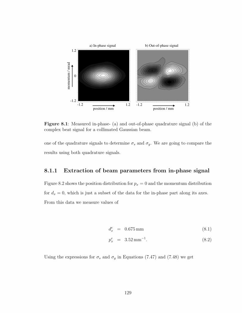
1.2

-1.2

0

1.2-1.2 1.2-1.2position / mm position / mm

mom

entu

m /

mra

d

a) In-phase signal b) Out-of-phase signal

Figure 8.1: Measured in-phase- (a) and out-of-phase quadrature signal (b) of thecomplex beat signal for a collimated Gaussian beam.

one of the quadrature signals to determine σs and σg. We are going to compare the

results using both quadrature signals.

8.1.1 Extraction of beam parameters from in-phase signal

Figure 8.2 shows the position distribution for px = 0 and the momentum distribution

for dx = 0, which is just a subset of the data for the in-phase part along its axes.

From this data we measure values of

dex = 0.675 mm (8.1)

pex = 3.52 mm−1. (8.2)

Using the expressions for σs and σg in Equations (7.47) and (7.48) we get

129

-1.2 1.20

p /k / mrad

S (p )BS (0)B

1

0

S (d )BS (0)B

1

0

d / mm

1.2-1.2

a) b)

0

e-1 e-1

x x

x x

2pxe

2dxe

Figure 8.2: (a) Measured position distribution for p = 0 and (b) momentumdistribution for x = 0 of the in-phase part of SB in Figure 8.1.

σs = 0.42 mm (8.3)

σg = 2.82 mm (8.4)

and therefore a global coherence for our SLD light leaving the collimating system

of

σglob =σg

σs

= 7.05. (8.5)

8.1.2 Extraction of beam parameters from out-of-phase sig-

nal

The measurement of dex and pe

x from the out-of-phase signal is done by measuring

the distance between the peaks and using Equations (7.39) and (7.40), as discussed

in Section 7.2.5. In Figure 8.1b, xm and pm are measured as shown in Figure 7.1:

130

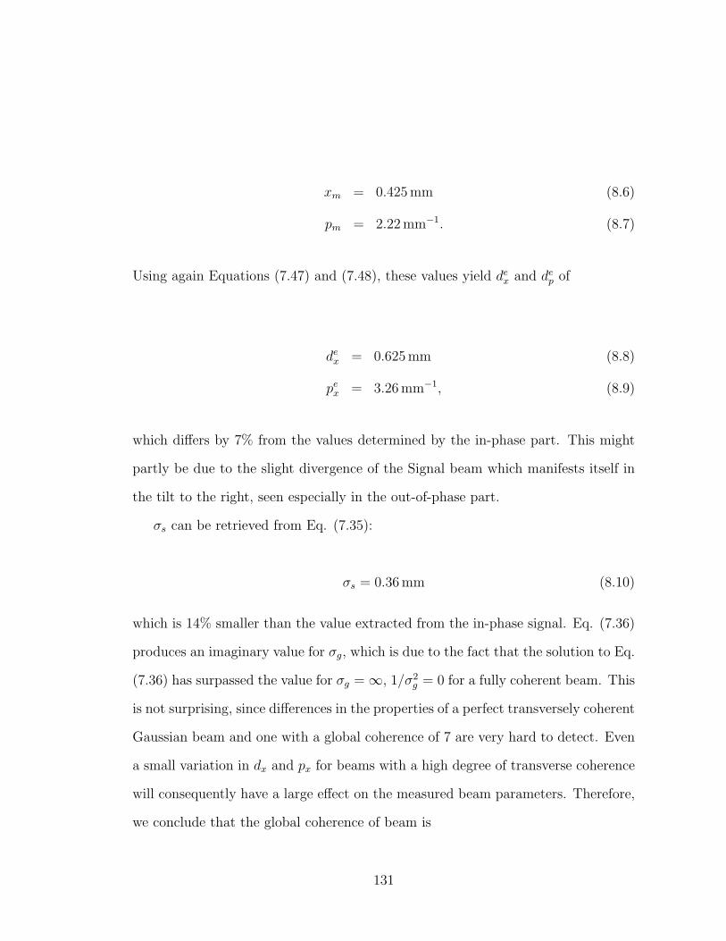
xm = 0.425 mm (8.6)

pm = 2.22 mm−1. (8.7)

Using again Equations (7.47) and (7.48), these values yield dex and de

p of

dex = 0.625 mm (8.8)

pex = 3.26 mm−1, (8.9)

which differs by 7% from the values determined by the in-phase part. This might

partly be due to the slight divergence of the Signal beam which manifests itself in

the tilt to the right, seen especially in the out-of-phase part.

σs can be retrieved from Eq. (7.35):

σs = 0.36 mm (8.10)

which is 14% smaller than the value extracted from the in-phase signal. Eq. (7.36)

produces an imaginary value for σg, which is due to the fact that the solution to Eq.

(7.36) has surpassed the value for σg = ∞, 1/σ2g = 0 for a fully coherent beam. This

is not surprising, since differences in the properties of a perfect transversely coherent

Gaussian beam and one with a global coherence of 7 are very hard to detect. Even

a small variation in dx and px for beams with a high degree of transverse coherence

will consequently have a large effect on the measured beam parameters. Therefore,

we conclude that the global coherence of beam is

131

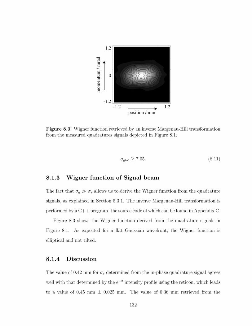
1.2

-1.2

0

1.2-1.2position / mm

mom

entu

m /

mra

d

Figure 8.3: Wigner function retrieved by an inverse Margenau-Hill transformationfrom the measured quadratures signals depicted in Figure 8.1.

σglob ≥ 7.05. (8.11)

8.1.3 Wigner function of Signal beam

The fact that σg À σs allows us to derive the Wigner function from the quadrature

signals, as explained in Section 5.3.1. The inverse Margenau-Hill transformation is

performed by a C++ program, the source code of which can be found in Appendix C.

Figure 8.3 shows the Wigner function derived from the quadrature signals in

Figure 8.1. As expected for a flat Gaussian wavefront, the Wigner function is

elliptical and not tilted.

8.1.4 Discussion

The value of 0.42 mm for σs determined from the in-phase quadrature signal agrees

well with that determined by the e−2 intensity profile using the reticon, which leads

to a value of 0.45 mm ± 0.025 mm. The value of 0.36 mm retrieved from the

132

out-of-phase signal on the other hand is off by 20 % from the reticon value, which

might be due to a slight curvature in the Signal beam wavefront which affects the

out-of-phase signal more than the in-phase signal.

The measured values for the transverse coherence length of σg ≥ 2.82 mm in the

in-phase signal and σg →∞ in the out-of-phase signal can not as easily be verified.

A good indicator to support the result that σg À σs is that in our experiments the

beat signal is almost invariant with respect to an inversion of the beam profile by

insertion of a 4f-system. Such an inversion affects not only the x− but also the

y−distribution of the field which most likely has a different global coherence length

due to the different collimation process in this direction.

The emitting area of our SLD is only 5×1 µm (width × height) [49] which leads

to a large angle of radiation. An estimate of the transverse coherence length can

be done using the Cittert-van Zernike theorem, assuming incoherent radiation from

the emitting area of the SLD, and taking into account the clipping of the field by

apertures: Light emitted from the emitting area of a width of w=5 µm propagates

approximately d=8 mm before entering the first collimation lens. At that distance,

the width of the coherence area is

σg ≈ λ

wd ≈ 1.1 mm. (8.12)

An aperture with a diameter of less than a millimeter clips the beam further in

order to improve the beam profile (see Section 6.3); therefore the transverse part of

the beam we use is well within its coherence area.

The fact that σg À σs is very convenient since it allows us to neglect the

exp[− (x1−x2)2

2σ2g

]-term in Eq. (3.2) which couples the Signal- and LO-fields due to

its cross-terms in the heterodyne scheme and makes it impossible to use their in-

133

dividual Wigner functions. Using the procedures outlined in Section 5.3.1 we can

then determine the Wigner function of the Signal field by inverse Margenau-Hill

transformation of the complex beat signal.

8.2 σg=∞, σs and R unknown

In this section, we are going to determine the radius of curvature and beam size of

a divergent Signal beam, using the out-of-phase quadrature signal as described in

Section 7.3.7. We detect and measure the beam reflected off the polished surface of

the sample container used in an experiment in Section 12.2.2 where we demonstrate

the change in sign of the radius of curvature of a field backscattered from a random

medium. The incident field, partially reflected from the surface of the sample cell,

serves as a reference in that experiment. The set-up modifications in the Signal arm

for the measurement of backscattered and reflected light are displayed in Figure 12.1.

The divergent beam is generated by placing a lens with a focal length of f=20

cm at a distance of 27 cm from the sample surface. The top row of Figure 12.5

shows the measured in-phase part, out-of-phase part and resulting Wigner function

of this field, reflected off the sample container. The rest of the figures shall not

concern us at the moment.

We extract the points of intersection dmx and pm

x of the tilted peaks in the out-

of-phase signals by plotting the momentum distribution at dx = 0 and the position

distribution at px = 0, as demonstrated in Section 7.3.7. Figure 8.4 shows both

plots.

We measure:

134

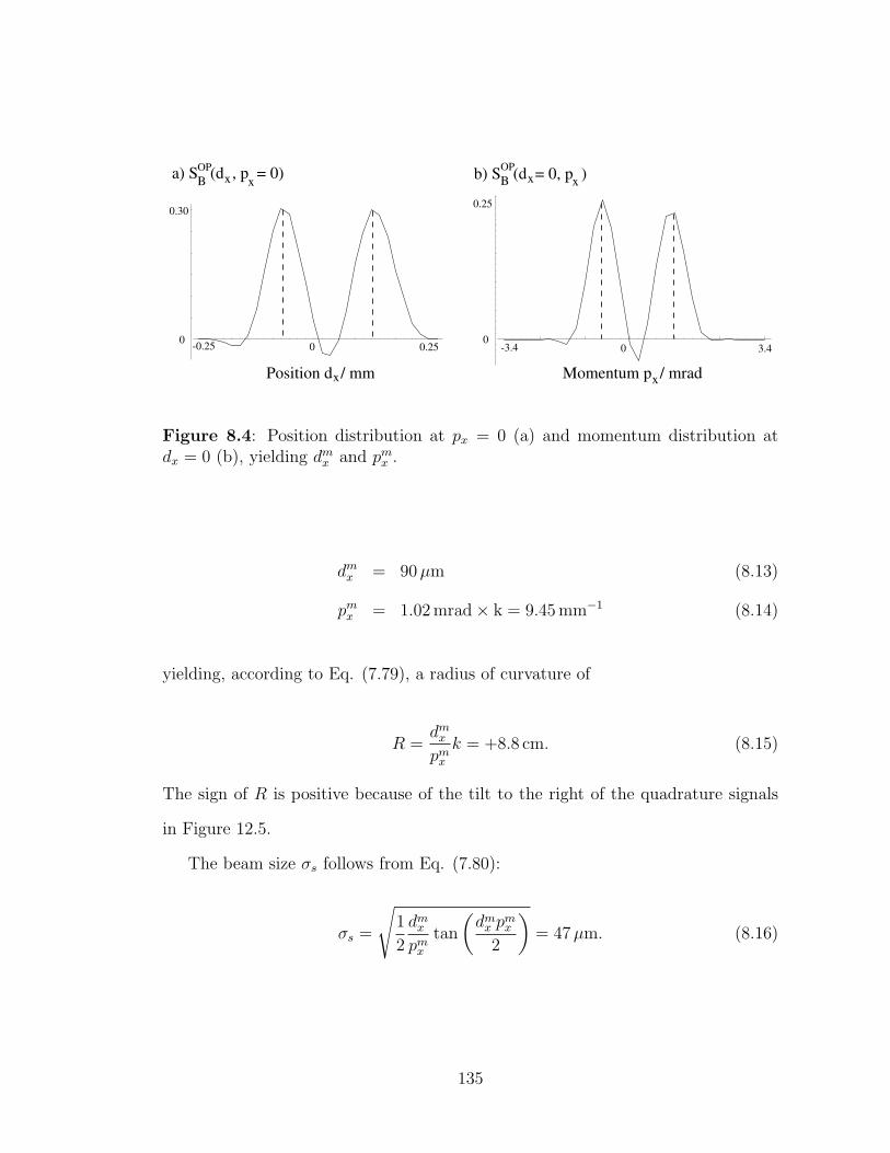
-0.25 0.250

Position d / mm

-3.4 3.40

Momentum p / mrad

0.250.30

0 0

x x

a) S (d , p = 0) B OP

x x b) S (d = 0, p ) B OP

x x

Figure 8.4: Position distribution at px = 0 (a) and momentum distribution atdx = 0 (b), yielding dm

x and pmx .

dmx = 90 µm (8.13)

pmx = 1.02 mrad× k = 9.45 mm−1 (8.14)

yielding, according to Eq. (7.79), a radius of curvature of

R =dm

x

pmx

k = +8.8 cm. (8.15)

The sign of R is positive because of the tilt to the right of the quadrature signals

in Figure 12.5.

The beam size σs follows from Eq. (7.80):

σs =

√1

2

dmx

pmx

tan

(dm

x pmx

2

)= 47 µm. (8.16)

135

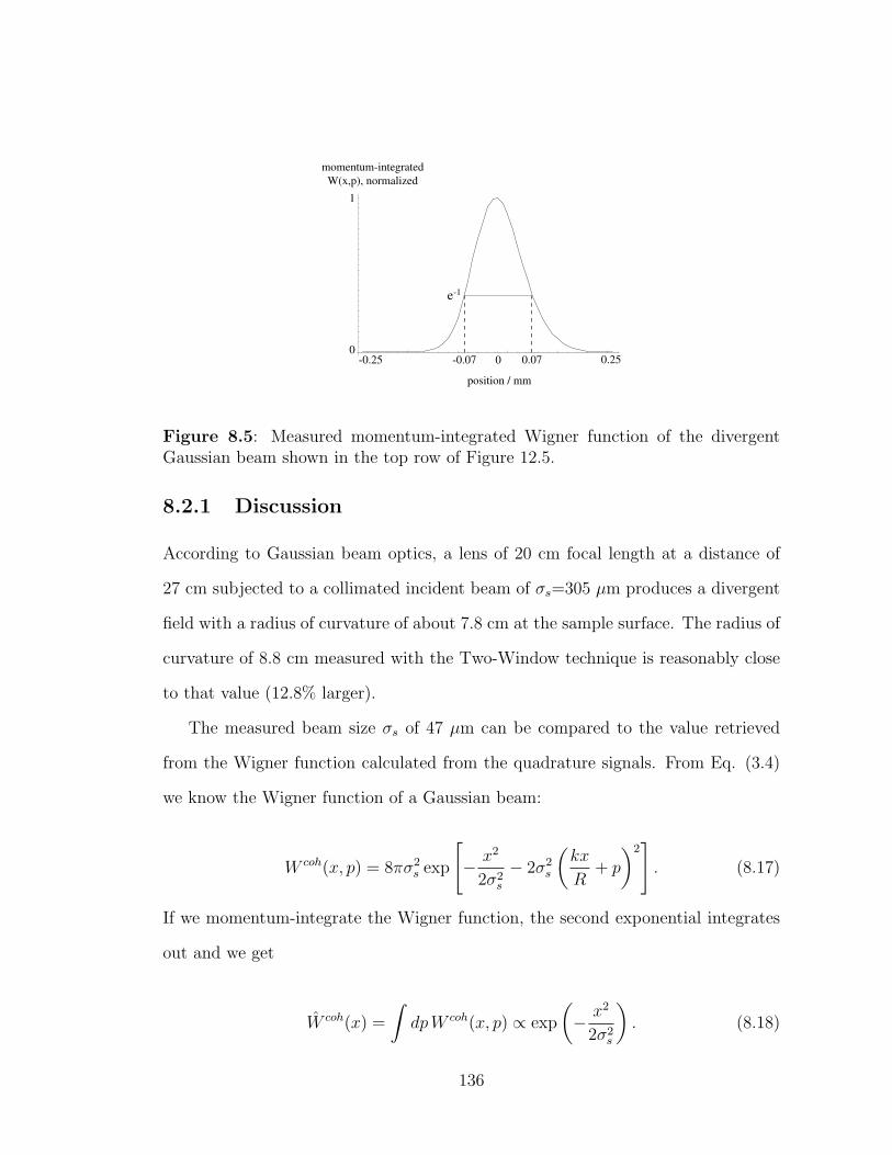
-0.25 0.250

1

0

momentum-integrated W(x,p), normalized

e-1

-0.07 0.07

position / mm

Figure 8.5: Measured momentum-integrated Wigner function of the divergentGaussian beam shown in the top row of Figure 12.5.

8.2.1 Discussion

According to Gaussian beam optics, a lens of 20 cm focal length at a distance of

27 cm subjected to a collimated incident beam of σs=305 µm produces a divergent

field with a radius of curvature of about 7.8 cm at the sample surface. The radius of

curvature of 8.8 cm measured with the Two-Window technique is reasonably close

to that value (12.8% larger).

The measured beam size σs of 47 µm can be compared to the value retrieved

from the Wigner function calculated from the quadrature signals. From Eq. (3.4)

we know the Wigner function of a Gaussian beam:

W coh(x, p) = 8πσ2s exp

[− x2

2σ2s

− 2σ2s

(kx

R+ p

)2]

. (8.17)

If we momentum-integrate the Wigner function, the second exponential integrates

out and we get

W coh(x) =

∫dp W coh(x, p) ∝ exp

(− x2

2σ2s

). (8.18)

136

From the spatial width of W coh(x) we can determine σs. Figure 8.5 shows the

measured W coh(x), retrieved from the measured Wigner function in Figure 12.5.

We measure σs = 50 µm, which agrees very well with the value of 47 µm determined

by the intersection points of the peaks in the out-of-phase quadrature signal.

8.3 Summary

The Two-Window technique enables the determination of the beam size σs, the

transverse coherence length σg and the radius of curvature R of the Signal beam by

means of either quadrature of the complex beat signal SB(dx, px). For a collimated

Signal beam, σs and σg can be extracted by determining the width of the in-phase

signal in position and momentum and also, more easily, from the location of the

clover-like peaks of the out-of-phase signal. From σs and σg the global coherence

σglob can be derived which is invariant for propagation through first-order optical

systems, in particular lenses and free space.

The measured beam sizes of σs = 0.42 mm (from in-phase signal) and 0.36 mm

(from out-of-phase signal) are in reasonable agreement with the value determined

by the reticon (0.45 mm ± 0.025 mm). A value for the transverse coherence length

of σg=2.82 mm was determined by the in-phase signal, the out-of-phase signal

yields a value of σg → ∞, resulting in a global coherence of σglob >7.05. Due

to the indistinguishability of beams with different but large global coherence, the

determination of an exact value for σg proves challenging.

For a Signal beam with finite radius of curvature and σg À σs, R and σs have

been determined from the locations of the clover-like peaks in phase-space for zero

position and momentum. The radius of curvature determined this way agrees with

the value calculated with Gaussian optics to within 13%. The beam-size σs was

137

measured to be 47 µm, which agrees very well with the value of 50 µm determined

by the spatial width of the momentum-integrated measured Wigner function of the

beam.

Unlike the One-Window technique previously used, the Two-Window technique

does not require the preparation of two identical beams. It employs a Dual-LO con-

sisting of a phase-locked set of a flat focused and a flat collimated LO which enables

the fast and accurate determination of beam-size, transverse coherence length and

radius of curvature of a Signal beam.

138

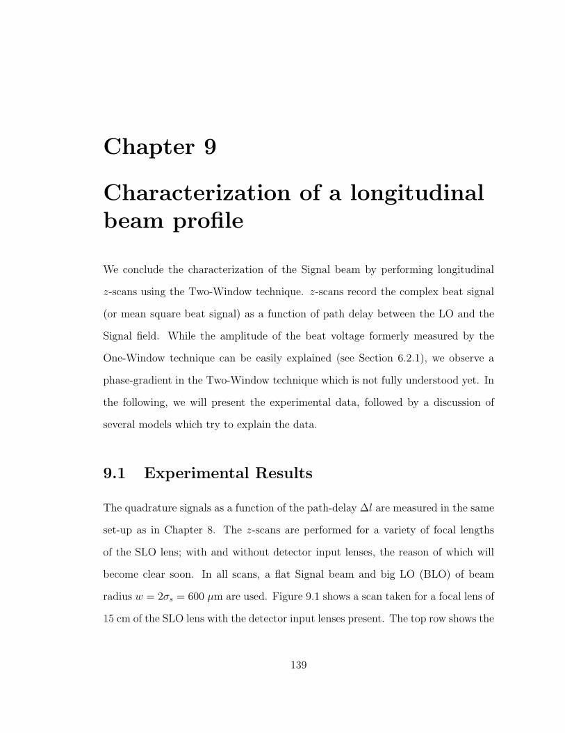
Chapter 9

Characterization of a longitudinalbeam profile

We conclude the characterization of the Signal beam by performing longitudinal

z-scans using the Two-Window technique. z-scans record the complex beat signal

(or mean square beat signal) as a function of path delay between the LO and the

Signal field. While the amplitude of the beat voltage formerly measured by the

One-Window technique can be easily explained (see Section 6.2.1), we observe a

phase-gradient in the Two-Window technique which is not fully understood yet. In

the following, we will present the experimental data, followed by a discussion of

several models which try to explain the data.

9.1 Experimental Results

The quadrature signals as a function of the path-delay ∆l are measured in the same

set-up as in Chapter 8. The z-scans are performed for a variety of focal lengths

of the SLO lens; with and without detector input lenses, the reason of which will

become clear soon. In all scans, a flat Signal beam and big LO (BLO) of beam

radius w = 2σs = 600 µm are used. Figure 9.1 shows a scan taken for a focal lens of

15 cm of the SLO lens with the detector input lenses present. The top row shows the

139

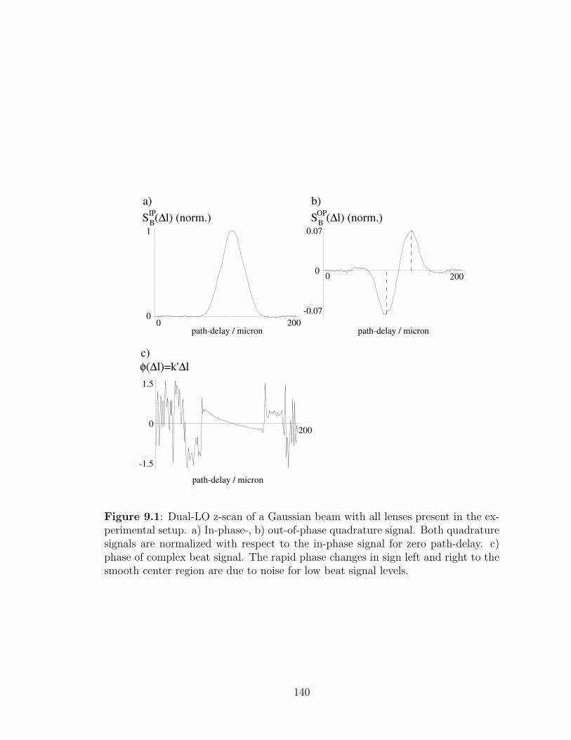
2000

path-delay / micron0 200

1

0

path-delay / micron

0

0.07

-0.07

S (∆l) (norm.)BIP S (∆l) (norm.)B

OP

0

-1.5

1.5

path-delay / micron

φ(∆l)=k'∆l

200

a) b)

c)

Figure 9.1: Dual-LO z-scan of a Gaussian beam with all lenses present in the ex-perimental setup. a) In-phase-, b) out-of-phase quadrature signal. Both quadraturesignals are normalized with respect to the in-phase signal for zero path-delay. c)phase of complex beat signal. The rapid phase changes in sign left and right to thesmooth center region are due to noise for low beat signal levels.

140

1

0

S (∆l) (norm.)BIP

0

0.04

-0.04

S (∆l) (norm.)BOP

φ(∆l)=k'∆l

0

-1.5

1.5

200

200path-delay / micron

path-delay / micron

path-delay / micron

200

a) b)

c)

Figure 9.2: Dual-LO z-scan of a Gaussian beam with SLO-lens present and bothinput lenses removed. a) In-phase-, b) out-of-phase quadrature signal. Both quadra-ture signals are again normalized with respect to the in-phase signal for zero path-delay. c) phase of complex beat signal.

in-phase- (a) and out-of-phase quadrature signal (b), normalized to the maximum

amplitude of the in-phase signal at zero path delay, over a path-delay range of 200

microns. c) shows the phase of the complex beat signal. The in-phase part looks

almost Gaussian, with an e−1 half-width of about ∆lB, as in the Single-LO z-scan

(Section 6.2.1).

Additional measurements without the input lenses and SLO-lenses of different

focal lengths yield results where the location of the out-of-phase peaks and ampli-

tude relative to the in-phase signal is similar to those measured in the first scan.

141

One example, which is shown in Figure 9.2, is a z-scan taken with the SLO-lens

present and both detector input lenses removed.

9.1.1 Discussion

The quadrature signals observed in Figure 9.1 and Figure 9.2 can be modelled by

the sum of a Gaussian amplitude and a phase gradient along the scanning direction;

i.e., a phase-difference between V SLOB and V BLO

B that changes linearly with the path-

difference ∆l between the respective LO and the Signal beam. In this case, the beat

voltages of the LOs can be written as

V BLOB (∆l) ∝ exp

[− ∆l2

2(∆lB)2

]exp(ik∆l + ik′1∆l) (9.1)

V SLOB (∆l) ∝ exp

[− ∆l2

2(∆lB)2

]exp(ik∆l + ik′2∆l). (9.2)

The first terms in both beat voltages in Equations (9.1) and (9.2) describe the

amplitude dependence; in the Single-Window technique this term is squared and

reproduces Eq. (6.1). The second term contains the phase contributions from the

path difference ∆l between the Signal beam and the respective LO and by the

additional phase gradients k′1 and k′2, which contribute to V BLOB and V SLO

B . The

complex beat signal is then:

SB(∆l) = V SLO∗B V BLO

B

= exp

[− ∆l2

(∆lB)2

]exp [i(k′1 − k′2)∆l] (9.3)

142

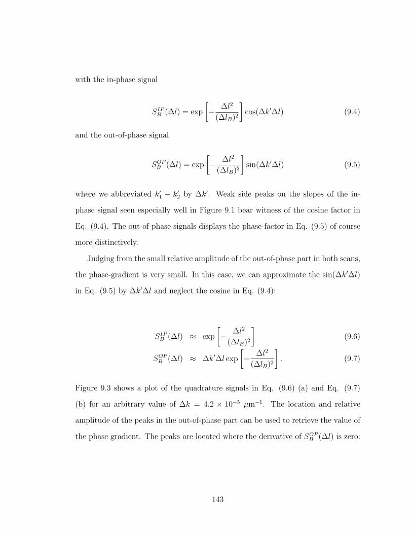
with the in-phase signal

SIPB (∆l) = exp

[− ∆l2

(∆lB)2

]cos(∆k′∆l) (9.4)

and the out-of-phase signal

SOPB (∆l) = exp

[− ∆l2

(∆lB)2

]sin(∆k′∆l) (9.5)

where we abbreviated k′1 − k′2 by ∆k′. Weak side peaks on the slopes of the in-

phase signal seen especially well in Figure 9.1 bear witness of the cosine factor in

Eq. (9.4). The out-of-phase signals displays the phase-factor in Eq. (9.5) of course

more distinctively.

Judging from the small relative amplitude of the out-of-phase part in both scans,

the phase-gradient is very small. In this case, we can approximate the sin(∆k′∆l)

in Eq. (9.5) by ∆k′∆l and neglect the cosine in Eq. (9.4):

SIPB (∆l) ≈ exp

[− ∆l2

(∆lB)2

](9.6)

SOPB (∆l) ≈ ∆k′∆l exp

[− ∆l2

(∆lB)2

]. (9.7)

Figure 9.3 shows a plot of the quadrature signals in Eq. (9.6) (a) and Eq. (9.7)

(b) for an arbitrary value of ∆k = 4.2 × 10−5 µm−1. The location and relative

amplitude of the peaks in the out-of-phase part can be used to retrieve the value of

the phase gradient. The peaks are located where the derivative of SOPB (∆l) is zero:

143

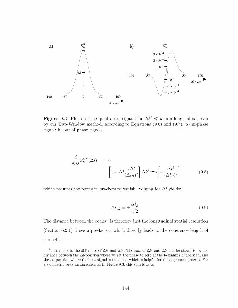
-100

1

0.5

-50 0 50 100

-100 -500

50 100

3 x10 -4

2 x10

10

-4

-4

-3 x10 -4

-2 x10 -4

-10 -4∆l / µm

∆l / µm

S OPBS B

IPa) b)

Figure 9.3: Plot o of the quadrature signals for ∆k′ ¿ k in a longitudinal scanby our Two-Window method, according to Equations (9.6) and (9.7). a) in-phasesignal; b) out-of-phase signal.

d

d∆lSOP

B (∆l) = 0

=

[1−∆l

2∆l

(∆lB)2

]∆k′ exp

[− ∆l2

(∆lB)2

](9.8)

which requires the terms in brackets to vanish. Solving for ∆l yields:

∆l1,2 = ±∆lB√2

. (9.9)

The distance between the peaks 1 is therefore just the longitudinal spatial resolution

(Section 6.2.1) times a pre-factor, which directly leads to the coherence length of

the light:

1This refers to the difference of ∆l1 and ∆l2. The sum of ∆l1 and ∆l2 can be shown to be thedistance between the ∆l-position where we set the phase to zero at the beginning of the scan, andthe ∆l-position where the beat signal is maximal, which is helpful for the alignment process. Fora symmetric peak arrangement as in Figure 9.3, this sum is zero.

144

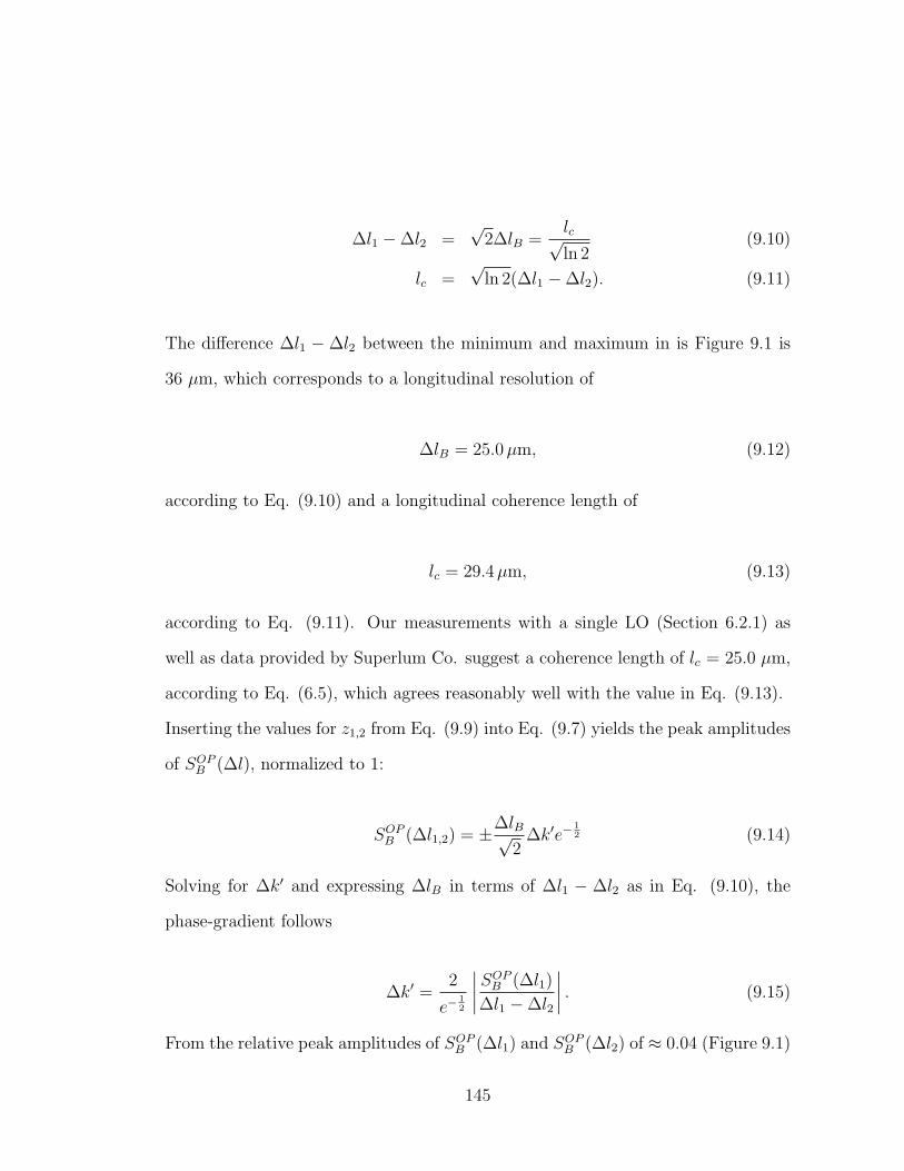
∆l1 −∆l2 =√

2∆lB =lc√ln 2

(9.10)

lc =√

ln 2(∆l1 −∆l2). (9.11)

The difference ∆l1 − ∆l2 between the minimum and maximum in is Figure 9.1 is

36 µm, which corresponds to a longitudinal resolution of

∆lB = 25.0 µm, (9.12)

according to Eq. (9.10) and a longitudinal coherence length of

lc = 29.4 µm, (9.13)

according to Eq. (9.11). Our measurements with a single LO (Section 6.2.1) as

well as data provided by Superlum Co. suggest a coherence length of lc = 25.0 µm,

according to Eq. (6.5), which agrees reasonably well with the value in Eq. (9.13).

Inserting the values for z1,2 from Eq. (9.9) into Eq. (9.7) yields the peak amplitudes

of SOPB (∆l), normalized to 1:

SOPB (∆l1,2) = ±∆lB√

2∆k′e−

12 (9.14)

Solving for ∆k′ and expressing ∆lB in terms of ∆l1 − ∆l2 as in Eq. (9.10), the

phase-gradient follows

∆k′ =2

e−12

∣∣∣∣SOP

B (∆l1)

∆l1 −∆l2

∣∣∣∣ . (9.15)

From the relative peak amplitudes of SOPB (∆l1) and SOP

B (∆l2) of ≈ 0.04 (Figure 9.1)

145

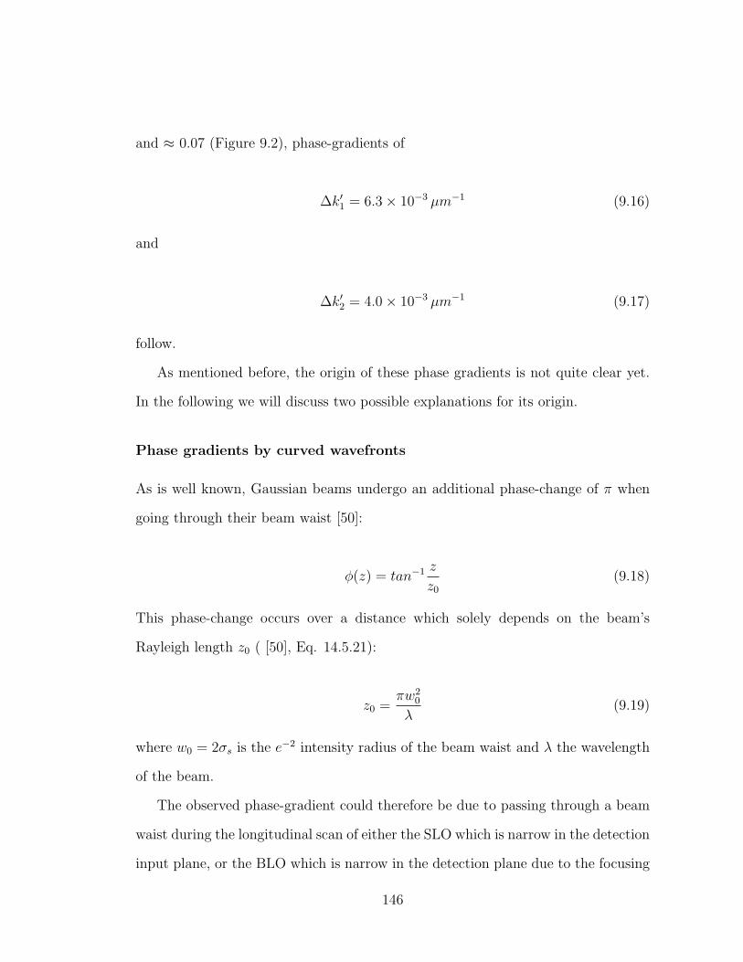
and ≈ 0.07 (Figure 9.2), phase-gradients of

∆k′1 = 6.3× 10−3 µm−1 (9.16)

and

∆k′2 = 4.0× 10−3 µm−1 (9.17)

follow.

As mentioned before, the origin of these phase gradients is not quite clear yet.

In the following we will discuss two possible explanations for its origin.

Phase gradients by curved wavefronts

As is well known, Gaussian beams undergo an additional phase-change of π when

going through their beam waist [50]:

φ(z) = tan−1 z

z0

(9.18)

This phase-change occurs over a distance which solely depends on the beam’s

Rayleigh length z0 ( [50], Eq. 14.5.21):

z0 =πw2

0

λ(9.19)

where w0 = 2σs is the e−2 intensity radius of the beam waist and λ the wavelength

of the beam.

The observed phase-gradient could therefore be due to passing through a beam

waist during the longitudinal scan of either the SLO which is narrow in the detection

input plane, or the BLO which is narrow in the detection plane due to the focusing

146

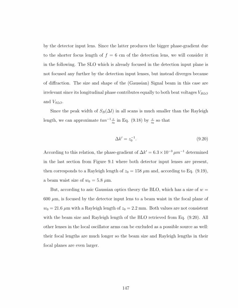
by the detector input lens. Since the latter produces the bigger phase-gradient due

to the shorter focus length of f = 6 cm of the detection lens, we will consider it

in the following. The SLO which is already focused in the detection input plane is

not focused any further by the detection input lenses, but instead diverges because

of diffraction. The size and shape of the (Gaussian) Signal beam in this case are

irrelevant since its longitudinal phase contributes equally to both beat voltages VBLO

and VSLO.

Since the peak width of SB(∆l) in all scans is much smaller than the Rayleigh

length, we can approximate tan−1 zz0

in Eq. (9.18) by zz0

so that

∆k′ = z−10 . (9.20)

According to this relation, the phase-gradient of ∆k′ = 6.3×10−3 µm−1 determined

in the last section from Figure 9.1 where both detector input lenses are present,

then corresponds to a Rayleigh length of z0 = 158 µm and, according to Eq. (9.19),

a beam waist size of w0 = 5.8 µm.

But, according to asic Gaussian optics theory the BLO, which has a size of w =

600 µm, is focused by the detector input lens to a beam waist in the focal plane of

w0 = 21.6 µm with a Rayleigh length of z0 = 2.2 mm. Both values are not consistent

with the beam size and Rayleigh length of the BLO retrieved from Eq. (9.20). All

other lenses in the local oscillator arms can be excluded as a possible source as well:

their focal lengths are much longer so the beam size and Rayleigh lengths in their

focal planes are even larger.

147

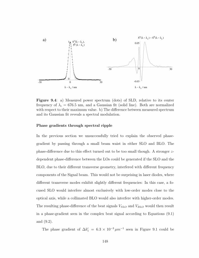
-30 300

1

0-0.03

0.05

-30 300

λ − λ / nmc

S (λ − λ ) − S (λ − λ )cex th

c

S (λ − λ ), S (λ − λ )

cex

thc

λ − λ / nmc

a) b)

Figure 9.4: a) Measured power spectrum (dots) of SLD, relative to its centerfrequency of λc = 676.5 nm, and a Gaussian fit (solid line). Both are normalizedwith respect to their maximum value. b) The difference between measured spectrumand its Gaussian fit reveals a spectral modulation.

Phase gradients through spectral ripple

In the previous section we unsuccessfully tried to explain the observed phase-

gradient by passing through a small beam waist in either SLO and BLO. The

phase-difference due to this effect turned out to be too small though. A stronger z-

dependent phase-difference between the LOs could be generated if the SLO and the

BLO, due to their different transverse geometry, interfered with different frequency

components of the Signal beam. This would not be surprising in laser diodes, where

different transverse modes exhibit slightly different frequencies: In this case, a fo-

cused SLO would interfere almost exclusively with low-order modes close to the

optical axis, while a collimated BLO would also interfere with higher-order modes.

The resulting phase-difference of the beat signals VSLO and VBLO would then result

in a phase-gradient seen in the complex beat signal according to Equations (9.1)

and (9.2).

The phase gradient of ∆k′1 = 6.3 × 10−3 µm−1 seen in Figure 9.1 could be

148

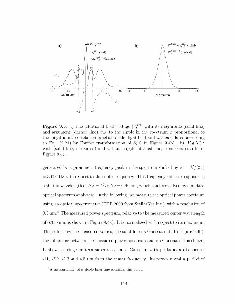
-100 0 100-50 50

∆l / micron-100 0 100-50 50

∆l / micron

|V | (solid)Bfri

|V + V | (solid)BfriB

Gauss 2

|V | (dashed)BGauss 2

0.074VBGaussa) b)

π π

−π −π

Arg(V ) (dashed)Bfri

Figure 9.5: a) The additional beat voltage |V friB | with its magnitude (solid line)

and argument (dashed line) due to the ripple in the spectrum is proportional tothe longitudinal correlation function of the light field and was calculated accordingto Eq. (9.21) by Fourier transformation of S(ν) in Figure 9.4b). b) |VB(∆l)|2with (solid line, measured) and without ripple (dashed line, from Gaussian fit inFigure 9.4).

generated by a prominent frequency peak in the spectrum shifted by ν = ck′/(2π)

= 300 GHz with respect to the center frequency. This frequency shift corresponds to

a shift in wavelength of ∆λ = λ2/c ∆ν = 0.46 nm, which can be resolved by standard

optical spectrum analyzers. In the following, we measure the optical power spectrum

using an optical spectrometer (EPP 2000 from StellarNet Inc.) with a resolution of

0.5 nm.2 The measured power spectrum, relative to the measured center wavelength

of 676.5 nm, is shown in Figure 9.4a). It is normalized with respect to its maximum.

The dots show the measured values, the solid line its Gaussian fit. In Figure 9.4b),

the difference between the measured power spectrum and its Gaussian fit is shown.

It shows a fringe pattern superposed on a Gaussian with peaks at a distance of

-11, -7.2, -2.3 and 4.5 nm from the center frequency. Its zeroes reveal a period of

2A measurement of a HeNe-laser line confirms this value.

149

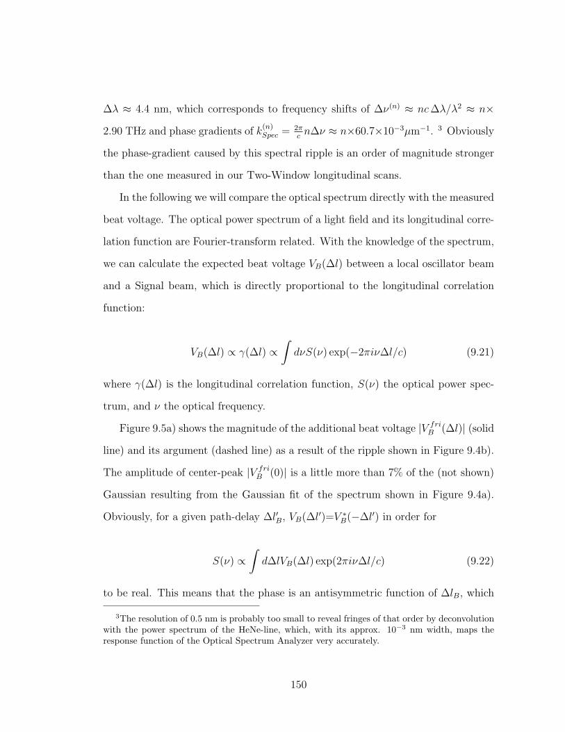
∆λ ≈ 4.4 nm, which corresponds to frequency shifts of ∆ν(n) ≈ nc ∆λ/λ2 ≈ n×2.90 THz and phase gradients of k

(n)Spec = 2π

cn∆ν ≈ n×60.7×10−3µm−1. 3 Obviously

the phase-gradient caused by this spectral ripple is an order of magnitude stronger

than the one measured in our Two-Window longitudinal scans.

In the following we will compare the optical spectrum directly with the measured

beat voltage. The optical power spectrum of a light field and its longitudinal corre-

lation function are Fourier-transform related. With the knowledge of the spectrum,

we can calculate the expected beat voltage VB(∆l) between a local oscillator beam

and a Signal beam, which is directly proportional to the longitudinal correlation

function:

VB(∆l) ∝ γ(∆l) ∝∫

dνS(ν) exp(−2πiν∆l/c) (9.21)

where γ(∆l) is the longitudinal correlation function, S(ν) the optical power spec-

trum, and ν the optical frequency.

Figure 9.5a) shows the magnitude of the additional beat voltage |V friB (∆l)| (solid

line) and its argument (dashed line) as a result of the ripple shown in Figure 9.4b).

The amplitude of center-peak |V friB (0)| is a little more than 7% of the (not shown)

Gaussian resulting from the Gaussian fit of the spectrum shown in Figure 9.4a).

Obviously, for a given path-delay ∆l′B, VB(∆l′)=V ∗B(−∆l′) in order for

S(ν) ∝∫

d∆lVB(∆l) exp(2πiν∆l/c) (9.22)

to be real. This means that the phase is an antisymmetric function of ∆lB, which

3The resolution of 0.5 nm is probably too small to reveal fringes of that order by deconvolutionwith the power spectrum of the HeNe-line, which, with its approx. 10−3 nm width, maps theresponse function of the Optical Spectrum Analyzer very accurately.

150

leads to a phase gradient close to zero path-delay, while its amplitude magnitude

is symmetric. Even though the phase-gradient is obviously much stronger than

the one observed in the z-scans, it might be possible that BLO and SLO inter-

fere with two parts of the Signal beam which have a slightly different spectral

composition, thereby causing a small phase-gradient in the complex beat signal

SB(∆l) ∝ V ∗SLOVBLO.

Figure 9.5b) shows the mean square beat signal |VB(∆l)|2 calculated from the

measured spectrum with (solid line) and without (dashed line) ripple in the spec-

trum. From the e−1-amplitude of the Gaussian fit of |VB(∆l)|2 a value of ∆lB=19.5

µm follows which is about 8% smaller than the values of 21.3 µm and 21.0 µm, de-

termined by the spectral values provided by Superlum Co. and a single-LO z-scan

in Section 6.2.1. This is probably due to the too small resolution of the optical spec-

trometer of 0.5 nm which broadens the measured spectrum and thereby decreases

the resulting ∆lB.

9.2 Summary

The measurement of the longitudinal distance between the peaks in the out-of-phase

signal, seen in Figure 9.1, enables the determination of the longitudinal coherence

to within 17.6%. This method requires a linear phase-gradient but is independent of

its magnitude as long as the phase-gradient is much smaller than the wavenumber of

the light. The origin of the phase gradient observed in our experiment is unknown.

It can not be explained by a narrow beam waist in either LO: The smallest values in

our experiment for the Rayleigh length z0 and the size of the beam waist w0 are still

an order of magnitude greater than those which would would cause the observed

phase gradient.

151

A much stronger phase gradient could be caused by spectral ripple pattern. The

phase-gradient we observe corresponds to a secondary peak in the spectrum of 0.46

nm next to the center peak. A measurement with an optical spectrometer with 0.5

nm resolution does not give any indication of such a peak though, but reveals a

ripple spectrum with spacings of about 4.4 nm. The corresponding phase gradient,

which is an order of magnitude larger than that measured by the z-scans, would only

be observed if the LOs would interfere with two different peaks in the spectrum.

Most likely though both LOs will interfere with parts of the Signal field of almost

the same spectral composition, except for a small difference which could possibly

cause the small phase gradient in the complex beat signal we observe.

The origin of the ripple in the spectrum itself is unknown; Superlum Co. gives

a value of 1% for the residual spectral modulation, and a maximum of 5%. Judging

from the peaks close to the center wavelength, the spectral modulation we measure

is about 4%. Transverse modes in the SLD could be a possible explanation, in case

the optical feedback is sufficiently high. Transverse modes differ by their spatial and

angular profile, so that LO beams with different beam profiles would interfere with

each mode to various extents, resulting in an overall phase-shift between the re-

spective beat voltages. But, in order to avoid stimulated emission, optical feedback

in SLDs is suppressed by anti-reflective coatings (reflectivity usually <0.01%, [51])

and a tilted or curved geometry of the active channel.

The pattern could also be caused by a parasitic Fabry-Perot interferometer of an

optical length of L = c2∆ν

=52 µm within (reflections in the semiconductor crystal)

or immediately after the SLD itself (SLD glass window). The frequency-selection

by a Fabry-Perot interferometer depends on the the angle of incidence, so that LOs

with different angular spectra will interfere with different frequency-components of

152

the Signal beam, also resulting in a approximately linear phase-gradient parallel to

scanning direction.

A more thorough investigation in a modified set-up could clarify the situation:

A measurement with a high-resolution optical spectrum analyzer space-integrated

over the beam profile should detect all side-peaks. Also, z-scans performed with

two small local oscillator beams at a variable, pre-selected transverse distance, su-

perposed with a collimated Signal beam, could potentially enable the mapping of

the spatial distribution of spectral features. In lasers, such a measurement could be

used to map the spatial profile and frequencies of transverse modes.

153

Chapter 10

Scattering theory

10.1 Introduction

Scattering in random media plays an important part in many fields of science.

In meteorology, electromagnetic waves are used to measure the properties of the

atmosphere by investigating the reflection off turbulent layers of air, rain, hail and

snow. In oceanography, particles in the ocean and fish swarms can be detected and

analyzed. In astronomy, scattering theory of light is used to model asteroid belts,

the rings and outer layers of the gas planets in our solar system and the interior of

stars. Another field where scattering theory plays an important role is biophysics,

where many optical techniques exist to characterize biological tissue, in particular

in-vivo, as described in Chapter 2. In some cases, scattering by cells is an unwelcome

byproduct that can be suppressed by certain techniques. In other cases the scattered

light is detected and analyzed in order to gain information about the scatterers

themselves. In particular, the spatial and angular distribution of a field scattered

from a skin layer can provide useful information about an architectural atypia of its

skin cells, which is an indicator for or, for mild abnormalities, a potential precursor

to skin cancer. This provides the grounds for a new diagnostic tool which might

potentially replace the time-consuming and invasive biopsy of today. Scattering

154

*

*

*

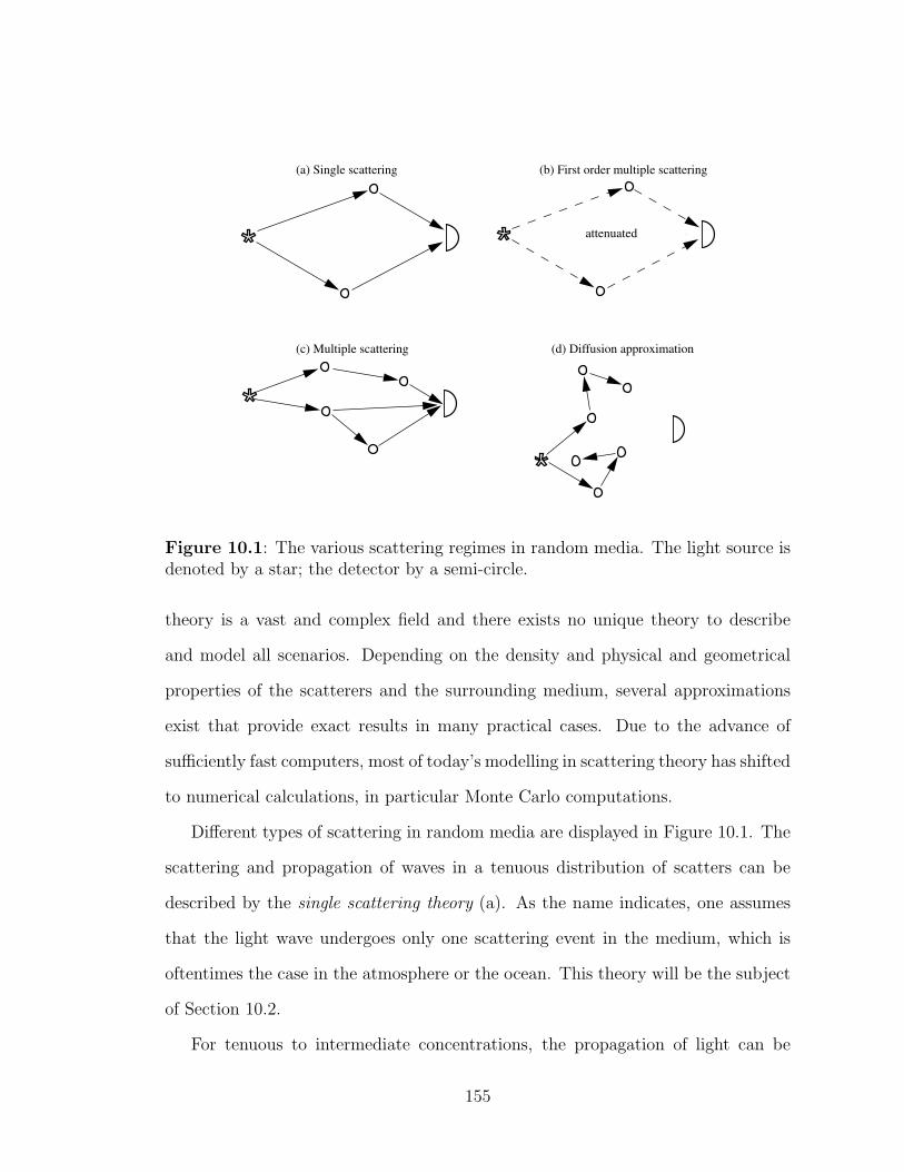
* attenuated

(a) Single scattering (b) First order multiple scattering

(c) Multiple scattering (d) Diffusion approximation

Figure 10.1: The various scattering regimes in random media. The light source isdenoted by a star; the detector by a semi-circle.

theory is a vast and complex field and there exists no unique theory to describe

and model all scenarios. Depending on the density and physical and geometrical

properties of the scatterers and the surrounding medium, several approximations

exist that provide exact results in many practical cases. Due to the advance of

sufficiently fast computers, most of today’s modelling in scattering theory has shifted

to numerical calculations, in particular Monte Carlo computations.

Different types of scattering in random media are displayed in Figure 10.1. The

scattering and propagation of waves in a tenuous distribution of scatters can be

described by the single scattering theory (a). As the name indicates, one assumes

that the light wave undergoes only one scattering event in the medium, which is

oftentimes the case in the atmosphere or the ocean. This theory will be the subject

of Section 10.2.

For tenuous to intermediate concentrations, the propagation of light can be

155

approximated by first-order multiple scattering (b) where also only one scattering

event is considered but with the path to and from the scatterer weighted by an

attenuation factor.

For intermediate concentrations, multiple scattering events are taken into ac-

count (c). One approach for this very complex problem is the Transfer theory, also

called theory of radiative transfer, which focuses on the propagation of intensities at

intermediate densities and provides a good approximation for many situations. This

theory will be the described in Section 10.3.1. Another approach is the Multiple

Scattering theory, which approximates the electric field by recursively integrating

over a number of scattering events while omitting unlikely scattering sequences.

This theory will be briefly summarized in Section 10.3.2.

For sufficiently dense distributions of scatterers and a scattering coefficient with

low angular dependence, the propagation of photons can be approximated by a

Markovian random-walk which means the intensity distribution is described by the

isotropic diffusion equation (d). This diffusion theory will be presented in Sec-

tion 10.4. Most practical examples in the diffusion-approximation regime display

an incoherent light field emerging from the random medium, due to the rapid ran-

domization of the fields phase and amplitude. There are some interesting coherent

phenomena though, which have gained increasing attention since their realization

in optical experiments in the beginning of the 1980s. They base on interference

of waves counter-propagating through identical paths in the medium. The most

important examples of this kind are Anderson localization and Enhanced backscat-

tering, the latter of which is an important part of this thesis. They are described

in Chapter 11.

156

10.2 Single-scatter theory

Most scatterers can be approximated by spheres, especially when they appear in

great numbers and random orientations. All single-scattering approximations pre-

sented in the following calculate the far-field of the secondary field generated in a

sphere by an incident flat wave. Depending on the size and relative index of refrac-

tion of the sphere there are many approximations. A good reference for a detailed

treatment is [52]. In the following I will briefly describe the idea and the most

important results of each approximation.

10.2.1 Rayleigh scattering

Rayleigh scattering describes the case where the size of a particle is much smaller

than a wavelength. Let us again assume this particle to be a dielectric sphere. In

that case, at each instant in time the electric field within and near the particle can

be approximated by an electrostatic field. The scattered field then corresponds to

that of regular dipole. The differential cross-section is proportional to the square

of the volume and inversely proportional to the fourth power of the wavelength.

The latter is responsible for the blue sky, because blue light scatters more than red

light. Contrary to early beliefs, the molecules of air itself contribute to Rayleigh

scattering, not only water and ice particles. The Rayleigh scattering cross section

approximation is exact within 4% of the true value if the size of the particle is

smaller then 0.05λ [53].

157

10.2.2 Born approximation

The Born approximation, also known as Raleigh-Debye scattering, applies to scat-

terers whose relative dielectric constant is close to unity:

[εr(~r)− 1]kD ¿ 1, (10.1)

where D is the diameter of the particle and k the wavenumber. In this case the

electric field inside the particle is approximated by the incident field. The resulting

scattering amplitude takes on a very simple form; it is directly proportional to the

Fourier transform of εr(~r)− 1 as a function of the change in momentum during the

scattering process.

10.2.3 WKB interior wave number approximation

In the WKB approximation the field inside the particle is approximated as the in-

cident field propagating with the medium’s propagation constant without changing

direction on entry into the medium. The transmission coefficient is assumed to be

that for normal incidence. The necessary conditions for this approximation are

[εr(~r)− 1]kD À 1 (10.2)

εr(~r)− 1 < 1. (10.3)

The calculated absorption cross sections in this approximation are usually a little

larger than the true value.

158

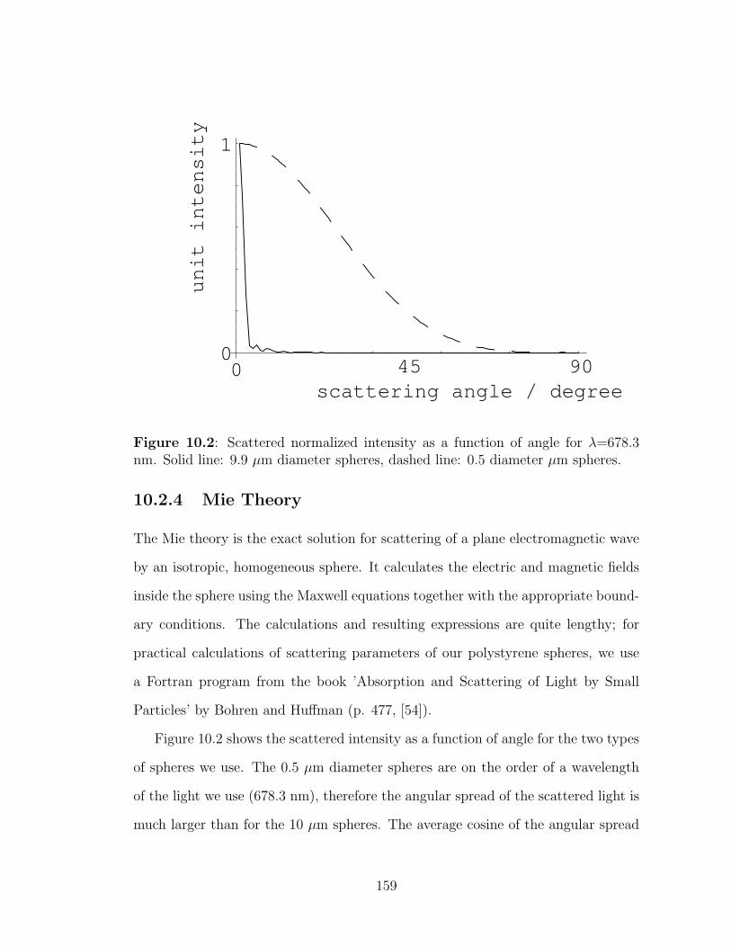
45 0 90

1

0

scattering angle / degree

unit intensity

Figure 10.2: Scattered normalized intensity as a function of angle for λ=678.3nm. Solid line: 9.9 µm diameter spheres, dashed line: 0.5 diameter µm spheres.

10.2.4 Mie Theory

The Mie theory is the exact solution for scattering of a plane electromagnetic wave

by an isotropic, homogeneous sphere. It calculates the electric and magnetic fields

inside the sphere using the Maxwell equations together with the appropriate bound-

ary conditions. The calculations and resulting expressions are quite lengthy; for

practical calculations of scattering parameters of our polystyrene spheres, we use

a Fortran program from the book ’Absorption and Scattering of Light by Small

Particles’ by Bohren and Huffman (p. 477, [54]).

Figure 10.2 shows the scattered intensity as a function of angle for the two types

of spheres we use. The 0.5 µm diameter spheres are on the order of a wavelength

of the light we use (678.3 nm), therefore the angular spread of the scattered light is

much larger than for the 10 µm spheres. The average cosine of the angular spread

159

for a 0.5 µm sphere is 〈cos θ〉 = 0.805, for a 10 µm sphere it is 〈cos θ〉 = 0.901.

Due to diffraction, the scattering cross-section of our spheres deviates from the

’classical’ cross-section that would be expected for particles. This is taken into

account by a correction factor Qsca so that the true cross section is Qscaπr2sph. For

0.5 µm diameter spheres, Qsca = 0.515, resulting in a scattering cross-section of

σs=0.101 µm2, for 10 µm diameter spheres Qsca = 1.993, leading to a cross-section

of σs=156.5 µm2.

10.3 Multiple Scattering

10.3.1 Transfer theory

Transfer theory, also called radiative transfer theory, is appropriate in the multiple-

scattering regime (see Figure 10.1(c)). It deals with the transport of energy in

random media containing particles and does not include interference or diffraction

effects, except for those affecting the single particle scattering characteristics. Also,

no correlation between fields is assumed, allowing for the superposition of intensities.

Transfer theory produces a differential equation, commonly referred to as equation

of transfer, which is equivalent to Boltzmann’s equation. The specific intensity

I(~r, s) is the quantity propagated in Transfer theory; it is the intensity per solid

angle and frequency at a given position and is measured in Wm2 sr Hz

.

The general form of the equation of transfer is

dI(~r, s)

ds= −ρσtI(~r, s) +

ρσt

4π

∫

4π

p(s, s′)I(~r, s)dω + ε(~r, s) (10.4)

which describes the change of I(~r, s) as it travels along a path ds. The first term

on the right-hand side describes the attenuation, which is proportional to the den-

160

sity of scatterers ρ and their total cross-section σt, which includes absorption and

scattering. The second term describes light scattered into the path of propagation

from all directions. It is proportional to ρσs since it is the scatterers in the path of

propagation that deflect the light. It is also proportional to the integral over the

specific intensities coming from all directions weighted by the phase-function p(s, s′)

which is the probability for a photon to be scattered from direction s′ into direction

s. The final term describes a potential source term. An exact analytical solution is

possible only for certain simple geometries and phase-functions. In cases where the

volume density is less then 0.1%, the second term can be simplified by assuming

that the light going to be scattered into the path s has to come from the reduced

incident intensity itself, rather than from diffuse light coming from all directions.

10.3.2 Twersky’s theory

Twersky’s integral is an iterative method where the field incident on a scatterer is

expressed as the field incident on the sample plus the field scattered from all other

scatterers [52]. The field scattered from that scatterer is in turn used to calculate

the field incident on all other scatterers. In order to simplify the iteration procedure,

certain unlikely scattering sequences are neglected. For practical calculations, the

sums are replaced by integrals.

10.4 Diffusion theory

For volume densities much greater than 1%, which is the case for all samples we use

for enhanced backscattering, the diffusion approximations provides good results.

The assumption here is that the diffuse intensity is scattered almost uniformly in

161

all directions, with a small overall flux in a direction s. This can be expressed as

Id(~r, s) ∝ Ud(~r) + c ~Fd(~r) · s, (10.5)

where Ud(~r) = 14π

∫4π

dω Id(~r, s) is the average diffuse intensity and

~Fd(~r) =∫4π

dω s Id(~r, s) is the diffuse flux vector. From the equation of transfer,

the diffusion equation can then be derived:

∇2Ud(~r)+3ρ2σtr[σsUri(~r)−σaUd(~r)] = − 3

4πρσtrE(~r)+

3

4π∇·

∫

4π

dω ε(~r, s) s, (10.6)

where σtr is the absorption cross section σa plus the scattering cross-section σs

corrected for anisotropic scattering and the ratio of the volume occupied by scat-

terers to the total volume. E(~r) is the angle-integrated source-function and ε(~r, s)

the source-terms due to the ballistic part of the incident field as well as additional

sources. Since the diffusion equation only holds if the light if sufficiently diffuse, it

is valid only far from the boundary and the source. Mathematically, this manifests

itself as follows: The boundary condition at a surface of a dense turbid medium,

Id(~r, s) = 0 when s is pointed inwards can not be fulfilled because the diffusion

equation describes the scalar field U rather then a vector field. Therefore, this

boundary condition needs to be replaced by one of the many approximations that

exist in that case. One of them requires that the total diffuse flux inwards be zero:

∫

2π

dω Id(~r, s) (s · n) = 0 (10.7)

where n is a unit vector normal to the surface and pointing inwards. Depending on

the anisotropy of the scatterers, this boundary condition takes on different forms for

162

the average diffuse intensity U . For special practical cases this boundary condition

simplifies. One example is the so-called Milne problem: For a semi-infinite slab

containing isotropic scatterers, an exact solution can be derived [52]. We will discuss

the time-dependent diffusion equation and present a solution for the Milne case in

Section 11.3. This section deals with the probability density for photon migration

which is proportional to the intensity of the light field.

In the following chapter I will describe Enhanced backscattering, which manifests

itself in the diffusion approximation regime but is nevertheless a coherent effect.

163

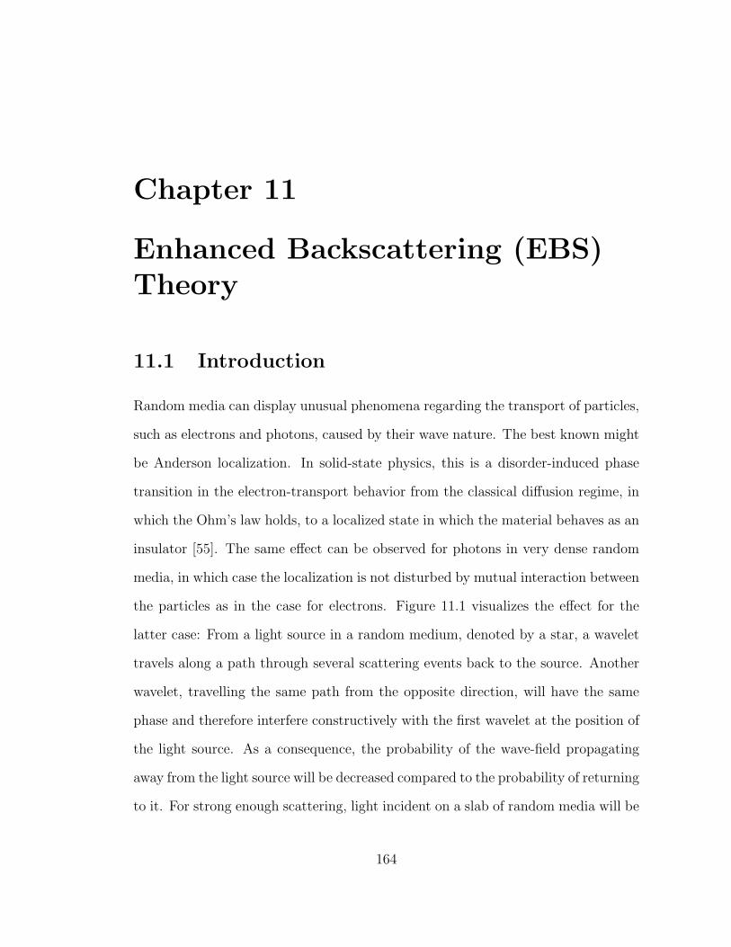
Chapter 11

Enhanced Backscattering (EBS)Theory

11.1 Introduction

Random media can display unusual phenomena regarding the transport of particles,

such as electrons and photons, caused by their wave nature. The best known might

be Anderson localization. In solid-state physics, this is a disorder-induced phase

transition in the electron-transport behavior from the classical diffusion regime, in

which the Ohm’s law holds, to a localized state in which the material behaves as an

insulator [55]. The same effect can be observed for photons in very dense random

media, in which case the localization is not disturbed by mutual interaction between

the particles as in the case for electrons. Figure 11.1 visualizes the effect for the

latter case: From a light source in a random medium, denoted by a star, a wavelet

travels along a path through several scattering events back to the source. Another

wavelet, travelling the same path from the opposite direction, will have the same

phase and therefore interfere constructively with the first wavelet at the position of

the light source. As a consequence, the probability of the wave-field propagating

away from the light source will be decreased compared to the probability of returning

to it. For strong enough scattering, light incident on a slab of random media will be

164

*

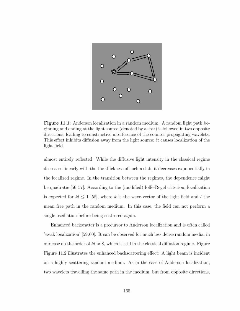
Figure 11.1: Anderson localization in a random medium. A random light path be-ginning and ending at the light source (denoted by a star) is followed in two oppositedirections, leading to constructive interference of the counter-propagating wavelets.This effect inhibits diffusion away from the light source: it causes localization of thelight field.

almost entirely reflected. While the diffusive light intensity in the classical regime

decreases linearly with the the thickness of such a slab, it decreases exponentially in

the localized regime. In the transition between the regimes, the dependence might

be quadratic [56,57]. According to the (modified) Ioffe-Regel criterion, localization

is expected for kl ≤ 1 [58], where k is the wave-vector of the light field and l the

mean free path in the random medium. In this case, the field can not perform a

single oscillation before being scattered again.

Enhanced backscatter is a precursor to Anderson localization and is often called

’weak localization’ [59,60]. It can be observed for much less dense random media, in

our case on the order of kl ≈ 8, which is still in the classical diffusion regime. Figure

Figure 11.2 illustrates the enhanced backscattering effect: A light beam is incident

on a highly scattering random medium. As in the case of Anderson localization,

two wavelets travelling the same path in the medium, but from opposite directions,

165

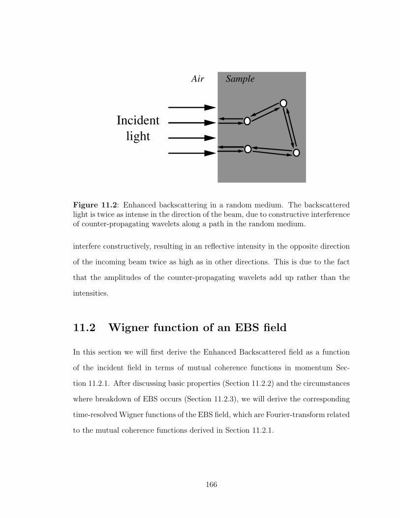
Incident light

Air Sample

Figure 11.2: Enhanced backscattering in a random medium. The backscatteredlight is twice as intense in the direction of the beam, due to constructive interferenceof counter-propagating wavelets along a path in the random medium.

interfere constructively, resulting in an reflective intensity in the opposite direction

of the incoming beam twice as high as in other directions. This is due to the fact

that the amplitudes of the counter-propagating wavelets add up rather than the

intensities.

11.2 Wigner function of an EBS field

In this section we will first derive the Enhanced Backscattered field as a function

of the incident field in terms of mutual coherence functions in momentum Sec-

tion 11.2.1. After discussing basic properties (Section 11.2.2) and the circumstances

where breakdown of EBS occurs (Section 11.2.3), we will derive the corresponding

time-resolved Wigner functions of the EBS field, which are Fourier-transform related

to the mutual coherence functions derived in Section 11.2.1.

166

k0

kf

k' (time-rev.)f

k' (time-rev.)0

r r

rrr

kk

k

k1

2

34

a

bc

j

i

-k4

-k3

-k2

-k1

Figure 11.3: Random path and its time-reversed counterpart in a random mediumfor an arbitrary incident wave: the rays ~k0 and ~k′0 which are incident on ~ri and ~rj

are no longer parallel, their amplitude is no longer equal. The outgoing field ~kf and~k′f becomes space-dependent and can no longer be fully described by a momentum-dependent intensity only.

11.2.1 Mutual coherence function of an EBS field

Figure 11.3 shows the intricacies of enhanced backscattering in more detail: the

incoming field with wave-vector ~k0 is incident on scatterers located at ~ri and ~rj in a

sample of random medium. We assume all scatterers in the sample to be point-like

and lossless. The relation between the momentum component of the field scattered

by a single scatterer ~k and of the incident field ~k′ can be described by a scattering

matrix.1 For the simple case of elastic scattering off a point scatterer at position ~r,

the scattering matrix Sk,k′(r) can be approximated by a position dependent phase

shift, weighted by a term describing the angular dependence:

S~k,~k′(~r) = S~k,~k′ei(~k′−~k)·~r (11.1)

1Here and in the following a prime ′ will mark fields and rays before scattering.

167

S~k′,~k=S ~−k, ~−k′ is time-reversal invariant, which means that the scattering character-

istics remain unchanged if we interchange incoming and outgoing wavevectors. The

amplitude of the field following a ray path with wavevector ~k0 which scatters first

at ~ri and exits with wavevector ~kf after scattering at ~rj is therefore given by

Aj = S ~kf~k4S ~k4

~k3S ~k3

~k2S ~k2

~k1S ~k1

~k0

× ei ~rj ·( ~k4− ~kf )+i ~rc·( ~k3− ~k4)+i ~rb·( ~k2− ~k3)+i ~ra·( ~k1− ~k2)+i~ri·( ~k0− ~k1)A′i (11.2)

= Pi,j(α)ei( ~k0·~ri− ~kf ·~rj)A′i (11.3)

where A′i and Aj are the complex amplitudes of the ray incident at ~ri and exiting

at ~rj,

Pj,i(α) = S ~kf~k4S ~k4

~k3S ~k3

~k2S ~k2

~k1S ~k1

~k0ei ~k4·(~rj−~rc)+i ~k3·(~rc−~rb)+i ~k2·(~rb− ~ra)+i ~k1·( ~ra−~ri). (11.4)

and α denotes the sequence of scatterers at locations ~ri, ~ra...~rc, ~rj that determine

the path and the direction of travel in the medium. Pj,i(α) = |Pj,i(α)| exp(iφj,i) is

called an probability amplitude by some authors [61] since it is a measure for the

probability that a given loop between ~ri and ~rj has acquired a phase φi,j and its

square magnitude enters the intensity.

Similarly, the ray entering at ~rj and exiting at ~ri, i.e. the ray counter-propagating

the one in Eq. (11.3) is given by

168

Ai = S ~kf~−k1

S ~−k1~−k2

S ~−k2~−k3

S ~−k3~−k4

S ~−k4~k0

× ei~ri·( ~−k1− ~kf )+i ~ra·( ~−k2+ ~k1)+i ~rb·( ~−k3+ ~k2)+i ~rc·( ~−k4+ ~k3)+i ~rj ·( ~k0+ ~k4)A′j

(11.5)

= Pi,j(αT )ei( ~k0·~rj− ~kf ·~ri)A′j (11.6)

where Ai, A′j and Pi,j(αT ) are defined accordingly, with αT denoting the same

scatterer sequence as α, travelled from the opposite direction. By comparison of

the phase-terms defining Pi,j and Pj,i it can be seen that Pi,j(αT )=Pj,i(α).

The mutual coherence function in momentum space resulting from all loops is

the sum of Equations (11.3) and (11.6), summed over all possible starting points,

paths and incident wavevectors:

〈E∗(~kf1)E(~kf2)〉 =∑

i,j,α,~k01

Pj,i(α)E0( ~k01)ei( ~k01·~ri− ~kf1·~rj)

×∑

l,m,α′,~k02

P∗l,m(α′)E∗0 ( ~k02)e−i( ~k02· ~rm− ~kf2·~rl) (11.7)

=∑

i,j,α,~k01

∑

l,m,α′,~k02

〈Pj,i(α)P∗l,m(α′)〉〈E0( ~k01)E∗0 ( ~k02)〉

× expi(~k01 · ~ri − ~kf1 · ~rj)− i(~k02 · ~rm − ~kf2 · ~rl) (11.8)

where we replaced the vectors A by electric fields E(k). E(k01) and E(k02) describe

the incoming field, E(kf1) and E(kf2) the outgoing field. The incoherent part repre-

sents the case where both electrical fields undergo the same sequence of scattering

in the same direction, i.e. i = m, j = l, α = α′. In this case Eq. (11.8) reduces to

169

〈E∗(~kf1)E(~kf2)〉incoh =∑

i,j,α,~k01,~k02

〈|Pj,i(α)|2〉〈|E∗0 (~k01)E0(~k02)〉

× expi[(~k02 − ~k01) · ~ri − (~kf2 − ~kf1) · ~rj] (11.9)

For the coherent part, the electrical fields go exactly opposite directions so that

i = l, j = m and Pij(αT ) = Pji(α), so that

〈E∗(~kf1)E(~kf2)〉coh =∑

i,j,α,~k01,~k02,α

〈|Pj,i(α)|2〉〈E∗0 (~k01)E0(~k02)〉

× expi[(~k02 + ~kf1) · ~ri − (~kf2 + ~k01) · ~rj]. (11.10)

All other contributions for arbitrary i, j, l, m, excluding Equations (11.9) and

(11.10), are responsible for a speckle pattern, which can be observed for stationary

scatterers and masks the enhanced backscatter peak. The speckle have a charac-

teristic width ∆θSp ∝ λ/L0, where L0, for limited-sized beams, is on the order of

the size of the coherence area or illuminated area, whichever is smaller. In the

introduction to this thesis, Chapter 1, we showed the Wigner function of a single

speckle coming from a piece of glass containing air bubbles. In the current setup,

the scattering polystyrene spheres which are suspended in a solution, are subject to

Brownian motion, so the speckle averages out and can therefore be neglected.

Before we go on with this calculation, let us consider the special case where a

plane wave is incident normal to the surface (~k01 = ~k02 ≡ ~k0) and we measure the

intensity as a function of angle (~kf1 = ~kf2 ≡ ~kf ). In this case, Equations (11.9) and

(11.10) reduce to

170

〈|E( ~kf )|2〉incoh =∑α,i,j

〈|Pj,i(α)|2〉〈|E0(~k0)|2〉 (11.11)

〈|E( ~kf )|2〉coh =∑α,i,j

〈|Pj,i(α)|2〉〈|E0(~k0)|2〉 cos[(~k0 + ~kf ) · ~ri − (~kf + ~k0) · ~rj],

(11.12)

yielding a total squared field of

〈|E( ~kf )|2〉 =∑α,i,j

〈|Pj,i(α)|2〉〈|E0(~k0)|2〉

× (1 + cos[(~k0 + ~kf ) · ~ri − (~kf + ~k0) · ~rj]), (11.13)

which displays the well known (1+ cos[(~k0 +~kf ) ·~ri− (~kf +~k0) ·~rj])-factor observed

in intensity measurements of collimated beams [59, 62, 63]. This factor becomes 2

when k0=−kf .

The width and length of the sample as well as the spatial characteristics of the

incident beam are generally large compared to the mean free path, so we can treat

the medium as semi-infinite. Then it is convenient to replace the sums in Eq. (11.8)

by integrals. For a given set of scatterers close to the surface at ~ri and ~rj, the sum of

the probabilities 〈|Pi,j(α)|2〉 over all possible loops α(~ri, ~rj) joining these scatterers

can be replaced by an integral over a probability density P (~rj − ~ri, t):2

2We directly assume P to be a function of the difference between ~rj and ~ri, which is justifiedin a semi-infinite random medium with homogeneous concentration of scatterers.

171

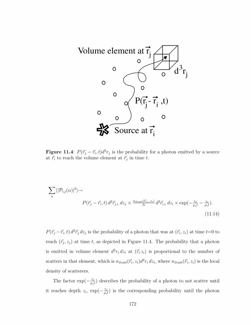
*d 3 r

P(r - r ,t)

Source at r i

j

Volume element at rj

ij

Figure 11.4: P (~rj − ~ri, t)d3rj is the probability for a photon emitted by a source

at ~ri to reach the volume element at ~rj in time t.

∑α

〈|Pi,j(α)|2〉→

P (~rj − ~ri, t) d2~rj⊥ dzj × nScatt(~ri⊥,zi)N

d2~ri⊥ dzi × exp(− zj

µj l− zi

µil).

(11.14)

P (~rj−~ri, t) d2~rj dzj is the probability of a photon that was at (~ri, zi) at time t=0 to

reach (~rj, zj) at time t, as depicted in Figure 11.4. The probability that a photon

is emitted in volume element d2ri dzi at (~ri zi) is proportional to the number of

scatters in that element, which is nScatt(~ri, zi)d2ri dzi, where nScatt(~ri, zi) is the local

density of scatterers.

The factor exp(− zj

µj l) describes the probability of a photon to not scatter until

it reaches depth zi, exp(− zj

µil) is the corresponding probability until the photon

172

reaches the surface after scattering at depth zj. l is the scattering mean free path

and µj and µi are the projections of the direction unit vectors of kj and ki on the

z-axis, assuming close to perpendicular incidence and emergence of the beam3. We

will incorporate this factor into P later on and therefore neglect displaying it for

now.

We will postpone the derivation of an expression for P (~rj−~ri, t) to Section 11.3.

The quantitatively exact integral form of Eq. (11.8), i.e., the correct prefactor, is

still subject to debate. The qualitatively correct expression follows from combining

Equations (11.8) and (11.14):

〈E∗(~kf1)E(~kf2)〉Back =

∫d3ri d

3rj P (~rj − ~ri, t)

×∫

d3k01 d3k02 〈E∗0 (~k01)E(~k02)〉

×

exp[i(~k02 + ~kf1) · ~ri − i(~kf2 + ~k01) · ~rj

]

+ exp[i(~k02 − ~k01) · ~ri − i(~kf2 − ~kf1) · ~rj

](11.15)

where we omitted constant prefactors.

11.2.2 Basic properties of an EBS field

The angular distribution of the intensity of the backscattered field as shown in Eq.

(11.13) is centered around the opposite direction of incidence (~kf = −~ki), where

the cosine is one. In this direction, the intensity is twice as big as the incoherent

3Actually the distance travelled by the wavelets before and after the scattering events differs fora given path and its time-reversed counterpart [64], which is negligible in the small angle regimewe are interested in. Therefore we just take one set of µi,j for both parts. Later on, we assumeµ ≈ 1.

173

background. The angular width of the Enhanced Backscatter peak depends on the

path lengths in the medium contributing to the enhanced backscatter effect and is,

for a given path length, approximately [62]

θc =λ

2π√

Dt(11.16)

Here, D is the diffusion constant of the photon migrating in the medium and t the

time passed after its incidence;√

Dt therefore is the typical distance of diffusion.

11.2.3 Breakdown of Enhanced Backscattering

There are many ways enhanced backscattering can break down. When the scatterers

move so fast that during the time the light needs to travel a given path, the path-

length changes by more than half the light’s wavelength, the wavelets coming from

opposite directions will not interfere constructively. In that case the EBS effect is

no longer observable. This does not pose a problem in our experiment though; even

with our smallest scatterers the comparably slow Brownian motion would require

a path length of the light in the medium of 3 meters [62] in order to destroy the

symmetry between counter-propagating wavelets, which is orders of magnitude more

than the submillimeter path-length we employ.

Other methods of destroying the Enhanced Backscatter effect break the sym-

metry between co- and counter-propagating waves. This works for example for

electrons, which are subjected to a magnetic field [55], but they have also been

experiments in the optical regime exploiting the Faraday effect [65].

174

11.2.4 Time-resolved Wigner function of an EBS field

The Wigner function formalism offers an attractive framework to describe Enhanced

Backscattering since it includes angular- and position information as well as phase

information. In this section, the time-resolved Wigner function of the backscattered

scalar field for a given incident light field will be derived. We again assume the case

of a light beam incident on the surface of a semi-infinite random medium. This

time we employ broadband light though, which enables us to selectively measure

the contributions by paths in the medium of a given length. The random medium

shall again consist of non-absorbing point-like scatterers.

We can transform the relation between the mutual coherence functions for the

incident and exiting fields in Eq. (11.15) into a relation between Wigner functions,

since the angular mutual coherence function is Fourier-transform related to the

Wigner function, as pointed out in Chapter 3:

W (~x, ~p) =

∫d3q

(2π)3exp(i~x · ~q) 〈E∗(~p +

~q

2)E(~p− ~q

2)〉 (11.17)

Solving for the mutual coherence function in momentum space yields:

〈E∗(~p +~q

2)E(~p− ~q

2)〉 =

∫d3x exp(−i~q · ~x)W (~x, ~p). (11.18)

We then define ~k01 = ~p1−~q1/2, ~k02 = ~p1 +~q1/2 for the incident field and ~kf1 = ~p2−~q2/2, ~kf2 = ~p2 +~q2/2 for the backscattered field in Eq. (11.15). This transformation

has a Jacobian of unity so that d3k01 d3k02 = d3p1 d3q1 and d3kf1 d3kf2 = d3p2 d3q2.

Replacing 〈E∗(~k01)E(~k02)〉 in Eq. (11.15) and integrating both sides according to

Eq. (11.17) yields

175

WBack(~x, ~p) =

∫d3~ri d

3~rj P (~rj − ~ri, t)

×∫

d3q2

(2π)3exp(i~x · ~q2)

×∫

d3p1 d3q1

∫d3x′ exp(−i~q1 · ~x′)W0(~x

′, ~p1)

× exp(i~q1 · ~ri − i~q2 · ~rj)

+ exp

[i

(~p1 + ~p2 +

~q1 − ~q2

2

)· ~ri − i

(~p1 + ~p2 +

~q2 − ~q1

2

)· ~rj

]

(11.19)

with the first exponential in the bottom line still the coherent and the second

exponential the incoherent part. The integrals with respect to ~q1 and ~q2 con-

tain only complex exponentials and can be directly solved, yielding delta functions

for the incoherent part (Equations (11.20),(11.21)) and coherent part (Equations

(11.22),(11.23)):

∫d3q2 exp[i~q2 · (~x− ~rj)] = (2π)3δ(~rj − ~x) (11.20)

∫d3q1 exp[i~q1 · (~ri − ~x′)] = (2π)3δ(~ri − ~x′) (11.21)

∫d3q2 exp

[i~q2 ·

(~x− ~ri + ~rj

2

)]= (2π)3δ

(~x− ~ri + ~rj

2

)(11.22)

∫d3q1 exp

[i~q1 ·

(−~x′ +

~ri + ~rj

2

)]= (2π)3δ

(~x′ − ~ri + ~rj

2

)(11.23)

By replacing the integrals in Eq. (11.19) with those delta functions the incoherent

and coherent parts of the Wigner function of the backscattered field result:

176

W IncohBack (~x, ~p) =

∫d3x′ d3p1 P (~x′ − ~x, t)W0(~x

′, ~p1)

=

∫d3x′ P (~x′ − ~x, t)W0(~x

′) (11.24)

where W0(~x′) is the momentum-integrated incident Wigner function4, and

WCohBack(~x, ~p) =

∫d3r′ d3p1 P (~r′, t) exp[−i(~p1 + ~p) · ~r′]W0(~x, ~p1). (11.25)

Even though the probability distribution P is not yet known, there are already some

interesting features discernible. The incoherent contribution W IncohBack in Eq. (11.24)

depends only on x and not an p, as is expected from incoherent fields. The spatial

characteristics of WCohBack in Eq. (11.25) are identical to W0. Its angular character-

istics are determined by P . In the next section we will derive an expression for P

in the diffusion approximation, which allows us to solve the integrals in Equations

(11.24) and (11.25) analytically.

11.3 The probability density P for photon migra-

tion

There exist many approximations for the probability density P , describing the sta-

tionary as well as the time-resolved behavior of photons in random media. The

stationary case has already been discussed in Section 10.4. As already pointed out

there, for sufficiently small size and large density of scatterers in the medium the

4Note that W has the unit power times momentum space volume = [Watt/m3], while the unitof W is just [Watts].

177

transport of the light can be described by the isotropic diffusion equation, at least

for distances from the surface large compared to the mean free path, where the

photons are sufficiently randomized. The Green’s function in the time-dependent

diffusion approximation regime has to obey [62]

(D∇2r +

∂

∂t)P (~r, ~r′; t) = δ(~r − ~r′)δ(t) (11.26)

where D is the diffusion constant. P (~r, ~r′; t) is then the probability distribution

for a photon to perform a random walk from ~r to ~r′ in time t without crossing the

surface. It would appear that the latter condition could be satisfied by requiring

P (~r, ~r′; t) to cancel at the surface. But, depending on the approach, P will cancel at

different surfaces outside the medium: For the exact solution of the Milne problem,

which treats the stationary mean-density of energy U(z) of a semi-infinite medium

containing isotropic scatterers as outlined in Section 10.4, P will cancel on the

plane z = −z0 with z0 = 0.7104...l. Within the more general stationary diffusion

approximation on the other hand, P will cancel on the plane z = −z0 with z0 = 23l

which is also valid for the time-dependent case. In this case, one obtains for P [62]:

P (~r, ~r′; t) =1

(4πDt)32

exp

(− ρ2

4Dt

)exp

[−(z − z′)2

4Dt

]− exp

[−(z + z′ + 2z0)

2

4Dt

].

(11.27)

It can readily be seen that the terms in brackets becomes zero for z = z′ = −z0.

Also, P depends only on ρ =| (~r − ~r′)⊥ | as expected from a semi-infinite medium

with translational invariance.

In our experiment, we measure the emerging field at the output plane, where

z = z′ = 0. Eq. (11.27) then reduces to

178

P (ρ; t) =1

(4πDt)32

exp

(− ρ2

4Dt

)[1− exp

(− z2

0

Dt

)]. (11.28)

For√

Dt À z0, which means that the light has diffused over much more than a

mean free path, the exponential can be expanded and the term in brackets becomes

approximatelyz20

Dt, so that Eq. (11.28) simplifies to:

P (ρ; t) =z20

(4π)32 (Dt)

52

exp

(− ρ2

4Dt

). (11.29)

In this expression and in the following we neglect the attenuation in z-direction

expressed by the last term in Eq. (11.14); we assume that the distance between the

sample surface and the first scatterer can be neglected.

In Section 11.4, the Wigner function for the backscattered field in the diffu-

sion approximation regime will be discussed, using the probability distribution for

photon migration in Eq. (11.29).

Note regarding the dimensionality of Wigner functions

Scattering in a bulk medium is a three-dimensional problem and needs to be treated

as such. On the other hand, we only detect the light field on the surface of the

sample, which is a two-dimensional problem.

For close to perpendicular incidence on and emission from a random medium,

the transverse mutual coherence function of the scattered field is determined by

the transverse properties of the incident beam but also by the path delay in z, as

discussed in the previous sections. The longitudinal mutual coherence function of

the backscattered field depends on the longitudinal properties of the incident beam

but also on the transverse location; inside the EBS cone it is different than out-

179

side. That means, that unlike for a Gaussian beam, the transverse and longitudinal

mutual coherence functions are not separable.

We extract the transverse Wigner function by keeping z constant, thereby defin-

ing the transverse plane we are interested in:

W (3D)(~r, ~p) → W⊥(~r⊥, ~p⊥, z = const, pz =ω

c) (11.30)

We can therefore use all results for three-dimensional Wigner functions from the

previous sections and just assume all vectors to be two-dimensional surface vectors.

11.4 EBS in the diffusion approximation regime

When we combine the result for the probability distribution P for photon migra-

tion from Eq. (11.29) and the general expression for the Wigner function of the

backscattered field in Equations (11.24) and (11.25), we get

W IncohBack (~x, ~p) ∝ z2

0

(4π)32 (Dt)

52

∫d2x′ exp

[−(~x− ~x′)2

4Dt

]W0(~x

′) (11.31)

WCohBack(~x, ~p) ∝ z2

0

Dt

∫d2p′ exp[−Dt(~p + ~p′)2]W0(~x, ~p′). (11.32)

We now have an expression for the Wigner function of the backscattered field as a

function of the Wigner function of the incident field alone. For the case of a Gaussian

beam incident on the sample, Equations (11.31) and (11.32) yield relatively simple

analytic expressions, as will be shown in Section 11.4.1.

180

In addition to the features of W IncohBack and WCoh

Back for general probability distri-

butions P already pointed out in Section 11.2.4, some other interesting properties

become visible for this special P : W IncohBack is the convolution of the incident Wigner

function and a Gaussian broadening term. It becomes broader with time as diffusion

progresses. For the hypothetical case of W0 = δ(~x), W IncohBack would be proportional

to P (~x, ~x0, t).

For the coherent part WCohBack(~x, ~p), the incident Wigner function is convolved

with a Gaussian term, which, unlike its counterpart in the incoherent term, be-

comes narrower with time, which causes the momentum distribution of the En-

hanced Backscatter Wigner function also to narrow with time. This Gaussian term

is maximal for ~p = −~p′, which agrees with the physical picture that enhanced

backscattering is most intense in the direction exactly opposite of the incident field.

11.4.1 EBS field for Gaussian incident beam

The Wigner function for the backscattered field with Gaussian transversely coher-

ent incident beam can be calculated straightforwardly by replacing the W0(~x, ~p) in

Equations (11.31) and (11.32) by Eq. (3.4):

W coh0 (~x, ~p) ∝ exp

− ~x2

2σ2s

− 2σ2s

(~k · ~xR

+ ~p

)2 (11.33)

where the vectors denote transverse components; we omit the ⊥ subscript for sim-

plicity. After some lines of straight-forward transformations we get for the incoher-

ent part

181

W Incoh,GaussianBack (~x, ~p) =

z20

(4π)32 (Dt)5/2

∫d2x′d2p′ exp

[−(~x− ~x′)2

4Dt

]W coh

0 (~x′, ~p′)

=

√π

2

z20

(Dt)3/2

1

2σ2s + 4Dt

exp

(− ~x2

2σ2s + 4Dt

)(11.34)

and for the coherent part

WCoh,GaussianBack (~x, ~p) =

z20

Dt

∫d2p′ exp[−Dt(~p + ~p′)2]W coh

0 (~x, ~p′)

=z20

Dt

π2

2σ2s + Dt

exp

− ~x2

2σ2s

−

(~k·~xR− ~p

)2

1Dt

+ 12σ2

s

. (11.35)

The combined Wigner function is then:5

W tot,GaussianBack (~x, ~p) = W Incoh,Gaussian

Back (~x, ~p) + WCoh,GaussianBack (~x, ~p)

=z20

(Dt)3/2

√π/2

2σ2s + 4Dt

exp

(− ~x2

2σ2s + 4Dt

)

+π2√

Dt

2σ2s + Dt

exp

− ~x2

2σ2s

−

(~k·~xR− ~p

)2

1Dt

+ 12σ2

s

(11.36)

5For both W , W →∞ for t →0 which is non-physical. This happens because our assumptionthat Dt À z2

0 is violated so the approximation leading to Eq. (11.29) breaks down and we needto replace z2

0Dt with 1− exp

(− z2

0Dt

).

182

11.5 Measured signal for the backscattered field

11.5.1 General expression for SincohB and Scoh

B

Now that we have an expression for the Wigner function of the backscattered field

we can calculate the mean square beat signal in the Single-Window technique and

the complex beat signal in the Two-Window technique that we expect to measure.

In Section 11.5.2 we will discuss the Single-Window case where all beams have a

circular Gaussian beam profile of the same size and the same radius of curvature.

Afterwards, the results can easily be adapted to the more general case. In Sec-

tion 11.5.3 we will derive the complex beat signal for the Two-Window technique.

All two-dimensional integrals in the following integrate over the transverse field.

For simplicity we will again omit the ⊥-subscript after each vector.

According to Eq. (4.25), the signal we measure is the convolution of the Wigner

function of the signal field, in the following denoted as WBack, and the Wigner

function of the local oscillator field, WLO:

SB( ~dx, ~dp) =

∫d2x d2p 〈WLO(~x− ~dx, ~p− ~px)WBack(~x, ~p, t)〉. (11.37)

As shown in Eq. (3.1), the Wigner function of the LO can be directly expressed in

terms of the corresponding electric field:

WLO(~x− ~dx, ~p + k~dp

f0

) =

∫d2ε

(2π)2exp

[i~ε

(~p + ~k ·

~dp

f0

)]

× E∗LO(~x +~ε

2− ~dx) ELO(~x− ~ε

2− ~dx). (11.38)

Here we just replaced (~x, ~p) by the coordinates shifted in phase-space (~x−~dx, ~p+k~dp

f0)

183

which describe the phase-space location of the LO relative to the Signal beam.

Incoherent part

We now insert Equations (11.34) and (11.38) into Eq. (11.37) and replace W coh0 (~x, ~p′)

in Eq. (11.34) according to Eq. (3.1), which yields

SincohB =

1

(2π)4

z20

(4π)3/2(Dt)5/2

∫d2x d2p d2x′d2p′d2ε d2ε′ exp[i~ε · (~p + ~px)]

× exp

[−(~x− ~x′)2

4Dt

]exp(i~ε′ · ~p′)

× 〈E∗LO(~x +~ε

2− ~dx)ELO(~x− ~ε

2− ~dx)E∗0 (~x′ +

~ε′

2)E0(~x

′ − ~ε′

2)〉.

(11.39)

As explained in Section 4.7, for heterodyne detection with transversely partially

coherent light it is necessary to ensemble average over E∗LO(x)ES(x′) rather than

E∗S(x)ES(x′) and E∗LO(x)ELO(x′) itself. Therefore we group the angled brackets in

Eq. (11.39) so that this is achieved. The integrals for p and p′ can be solved right

away:

∫d2p exp(i~ε · ~p) = (2π)2δ(~ε) (11.40)

∫d2p′ exp(i~ε′ · ~p′) = (2π)2δ(~ε′) (11.41)

(11.42)

so that Eq. (11.39) becomes

184

SincohB (~dx, ~dp) =

z20

(4π)3/2(Dt)5/2

∫d2x d2x′ exp

[−(~x− ~x′)2

4Dt

]

× 〈E∗LO(~x− ~dx)E0(~x′)〉〈ELO(~x− ~dx)E∗0 (~x′)〉

=z20

(4π)3/2(Dt)5/2

∫d2x d2x′ exp

[−(~x− ~x′)2

4Dt

]|〈E∗LO(~x− ~dx)E0(~x

′)〉|2.

(11.43)

Coherent part

For the coherent part we proceed similar to the incoherent part, except that we now

insert Equations (11.35) and (11.38) into Eq. (11.37). We get:

ScohB (~dx, ~dp) =

1

16π4

z20

Dt

∫d2x d2ε d2ε′

× 〈E∗LO(~x +~ε

2− ~dx)ELO(~x− ~ε

2− ~dx)E∗0 (~x +

~ε

2)E0(~x− ~ε′

2)〉

×∫

d2p d2p0 exp

[i~ε ·

(~p + k

~dp

f0

)]exp(i~ε′ · ~p0) exp[−Dt(~p + ~p0)

2].

(11.44)

The integrals over p and p0 can be solved right away:

∫d2p d2p0 exp(i~ε · ~p) exp(i~ε′ · ~p0) exp[−Dt(~p + ~p0)

2]

= exp(i~px · ~ε)∫

d2p exp(i~ε · ~p) exp(−i~ε′ · ~p)∫

d2p0 exp(i~ε′ · ~p0) exp[−Dt~p20]

=4π3

Dtexp(i~px · ~ε) exp

(− ~ε′2

4Dt

)δ(~ε− ~ε′). (11.45)

185

Inserting Eq. (11.45) into Eq. (11.44) and switching the angled brackets as in the

incoherent case, we get

ScohB ( ~dx, ~dp) =

z20

4π(Dt)2

∫d2x d2ε exp

[− ~ε2

4Dt− i~ε · ~dp

k

f0

]

× 〈E∗LO(~x− ~dx +~ε

2)E0(~x− ~ε

2)〉

× 〈ELO(~x− ~dx − ~ε

2)E∗0 (~x +

~ε

2)〉. (11.46)

Equations (11.43) and (11.46) are the basis for the calculations of the mean square

beat signal in the Single-Window technique and the complex beat signal in the

Dual-Window technique.

11.5.2 Single-Window technique

The mean square beat signal for the special case that LO and incident Signal beam

have an identical beam profile, has already been derived in [4, 5]. Since then, we

corrected the prefactor of the probability density P we use so that the mean square

signal now reads:

SSingleLOB (dx, dp, t) ∝

√4πδ2z2

0

(Dt)3/2exp

(− d2

x

a′2

)+

δ′2z20

(Dt)2exp

(−d2

x

a2− δ′2p2

x

),(11.47)

where 1/a2 = 1/(4σ2s) + 1/σ2

g , 1/δ2 = 1/(Dt) + 4/a2, a′2 = a2(Dt/δ2), and 1/δ′2 =

1/δ2 + 4k2σ2s/R

2. As in previous chapters, σs is the beam size, σg the transverse

coherence, and R the radius of curvature.

Since this thesis deals primarily with the Two-Window technique, we will not

186

get into the details of the Single-Window technique results and instead refer to the

aforementioned papers.

11.5.3 Dual-Window technique

The calculations of the mean square beat signal for the Dual-Window technique are

rather lengthy and not very instructional. I will therefore just mention the most

important steps and refer to Appendix B for details.

Incoherent part

For the incoherent part, we take Eq. (11.43) and adapt it to the dual-LO case. The

electric fields for LO and incident light are, as already shown in Eq. (5.1):

ELO(~x) ∝ exp

(− ~x2

4σ2sa

2

)+ βeiθ exp

(− ~x2

4σ2sA

2

)= Ea

LO(~x) + βeiθEALO(~x) (11.48)

with θ = ωt denoting the 3 kHz-phase-lock frequency between the LOs and β the

relative amplitude of the big LO with respect to the small LO; and the incident

beam is

E0(~x) ∝ exp

(− ~x2

4σ2sB

2+

ik

2RB2~x2

). (11.49)

A, a and B denote again the scaling factors of the big LO, small LO and signal

beam relative to the initial beam radius 2σs. The squared product of the electric

fields in Eq. (11.43) is then:

187

|〈E∗LO(~x1)E0(~x2)〉|2 = (〈Ea∗LO(~x1)E0(~x2)〉+ βeiθ〈EA∗

LO(~x1)E0(~x2)〉)

× (〈EaLO(~x1)E∗0 (~x2)〉+ βe−iθ〈EA

LO(~x1)E∗0 (~x2)〉) (11.50)

with ~x1=~x− ~dx and ~x2=~x′. Again, we detect the cross-terms only:

βeiθ〈EA∗LO(~x1)E0(~x2)〉〈Ea

LO(~x1)E∗0 (~x2)〉+ βe−iθ〈EALO(~x1)E∗0 (~x2)〉〈Ea∗

LO(~x1)E0(~x2)〉,(11.51)

the other terms average to zero. The second term in Eq. (11.51) is the complex

conjugate of the first, so we need to calculate the first term only. The in-phase

mean square beat signal will be twice the real part of the ensuing calculation; the

out-of-phase signal twice the imaginary part. The ensuing calculation is explicitly

shown in Appendix B; we will just show the result here. The complex beat signal

SincohB is then:

SincohB (dx) =

√π

4

z20

(Dt)3/2

1

(vB + v∗B)(vA + va)

× exp

(− d2

x1

vA+va+ 1

vB+v∗B+ 4Dt

). (11.52)

where

188

vA =1

4σ2sA

2(11.53)

va =1

4σ2sa

2(11.54)

vB =1

4σ2sB

2− ik

2RB(11.55)

(11.56)

The complex beat signal for the incoherently backscattered field is real. Therefore,

the out-of-phase quadrature signal is zero throughout phase-space. In reality, the

measured out-of-phase signal is never at exactly at 90 degree phase-shift with re-

spect to the center of the EBS cone in Signal phase-space, which leads to small

contributions from the incoherent background for the out-of-phase part as well.

The imaginary part of vB which contains the radius of curvature R of the Signal

field, cancels. This means that the properties of the incoherent background are

independent of the radius of curvature of the incident field, at least for an ideal

turbid medium.

Coherent part

For the calculation of the coherent part of the mean square beat signal, ScohB , we

start with Eq. (11.46), using the same expressions for E0 (Eq. (11.49)) and ELO

(Eq. (11.48)) as for the incoherent part. The detailed calculation is shown in

Appendix B. The resulting integral for ScohB is

189

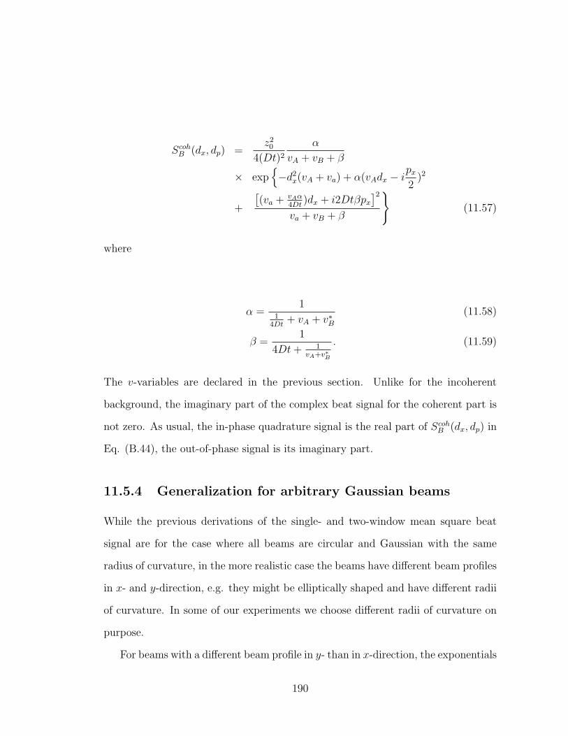
ScohB (dx, dp) =

z20

4(Dt)2

α

vA + vB + β

× exp−d2

x(vA + va) + α(vAdx − ipx

2)2

+

[(va + vAα

4Dt)dx + i2Dtβpx

]2

va + vB + β

(11.57)

where

α =1

14Dt

+ vA + v∗B(11.58)

β =1

4Dt + 1vA+v∗B

. (11.59)

The v-variables are declared in the previous section. Unlike for the incoherent

background, the imaginary part of the complex beat signal for the coherent part is

not zero. As usual, the in-phase quadrature signal is the real part of ScohB (dx, dp) in

Eq. (B.44), the out-of-phase signal is its imaginary part.

11.5.4 Generalization for arbitrary Gaussian beams

While the previous derivations of the single- and two-window mean square beat

signal are for the case where all beams are circular and Gaussian with the same

radius of curvature, in the more realistic case the beams have different beam profiles

in x- and y-direction, e.g. they might be elliptically shaped and have different radii

of curvature. In some of our experiments we choose different radii of curvature on

purpose.

For beams with a different beam profile in y- than in x-direction, the exponentials

190

in the final results remain the same, but the pre-factor pref must be replaced by√

prefxprefy, where prefx and prefy contain the direction-specific beam parameters

in x and y.

Misalignments in y-direction, both angular and positional, can be also be in-

cluded into the model simply by introducing equivalent expressions for dy and dp(y)

as for dx and dp.

191

Chapter 12

Enhanced Backscattering (EBS)Experiments

This chapter presents a study of measured time-resolved Wigner functions of En-

hanced Backscattering from a turbid medium. In the first section we briefly de-

scribe the adaptations to the experimental setup for the measurement of backscat-

tered light. Also we are going to discuss the properties and limitations of the turbid

medium we use: It consists of polystyrene spheres of 0.5 micron diameter suspended

in a neutral buoyancy solution.

In the second section we are going to present our experimental results; for a

collimated as well as a convergent and divergent incident beam and at various path

lengths in the medium. The Enhanced Backscatter cone for a curved incident wave-

front shows a reversal of radius of curvature, confirming for the first time directly the

phase-conjugating properties of a Enhanced Backscattering from a turbid medium.

In the third section we study the momentum distribution of the EBS peak as a

function of path-delay. We conclude this chapter with the discussion of the experi-

mental results, the comparison to the theoretical predictions outlined in Chapter 11,

and the summary.

192

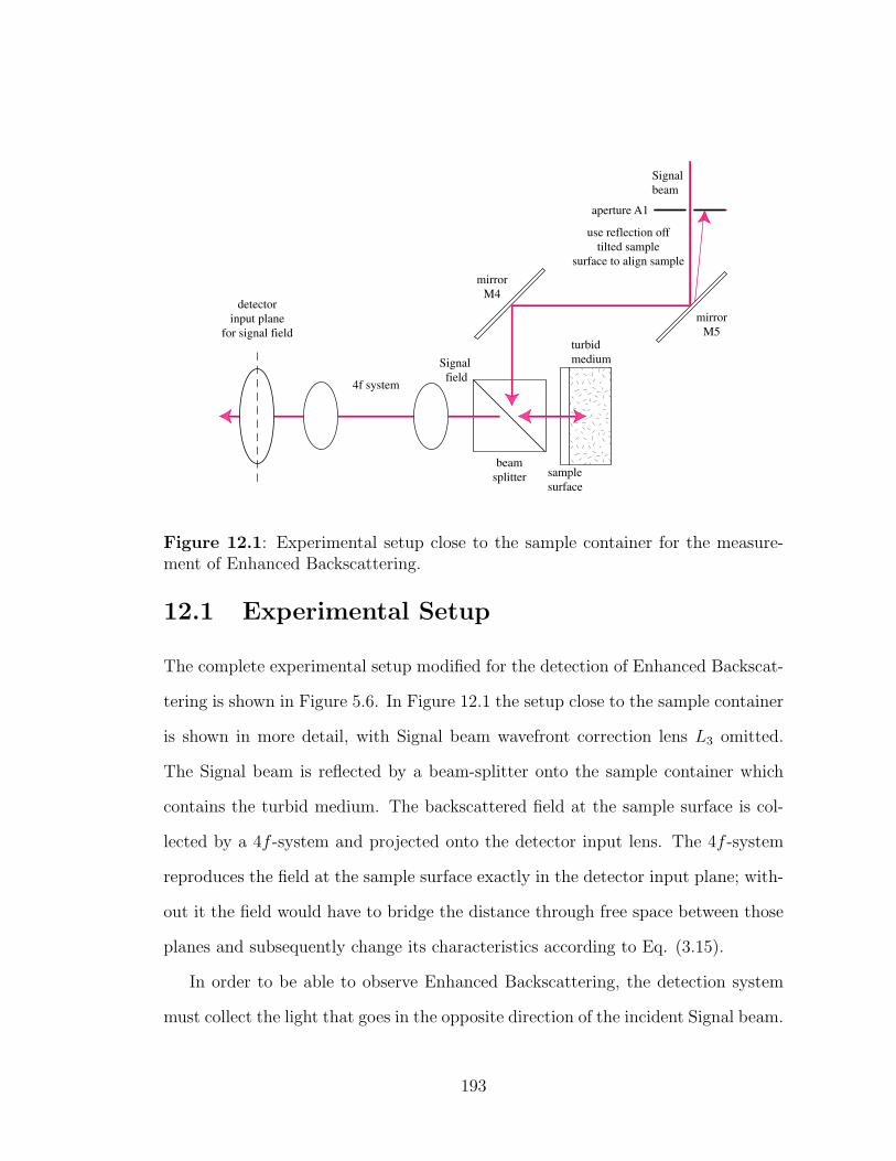
Signal field

sample surface

use reflection off tilted sample

surface to align sample

4f system

detector input plane

for signal field

Signal beam

turbid medium

beam splitter

mirror M4

mirror M5

aperture A1

Figure 12.1: Experimental setup close to the sample container for the measure-ment of Enhanced Backscattering.

12.1 Experimental Setup

The complete experimental setup modified for the detection of Enhanced Backscat-

tering is shown in Figure 5.6. In Figure 12.1 the setup close to the sample container

is shown in more detail, with Signal beam wavefront correction lens L3 omitted.

The Signal beam is reflected by a beam-splitter onto the sample container which

contains the turbid medium. The backscattered field at the sample surface is col-

lected by a 4f -system and projected onto the detector input lens. The 4f -system

reproduces the field at the sample surface exactly in the detector input plane; with-

out it the field would have to bridge the distance through free space between those

planes and subsequently change its characteristics according to Eq. (3.15).

In order to be able to observe Enhanced Backscattering, the detection system

must collect the light that goes in the opposite direction of the incident Signal beam.

193

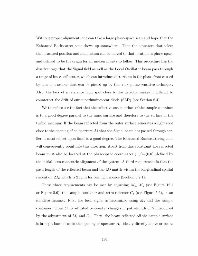
Without proper alignment, one can take a large phase-space scan and hope that the

Enhanced Backscatter cone shows up somewhere. Then the actuators that select

the measured position and momentum can be moved to that location in phase-space

and defined to be the origin for all measurements to follow. This procedure has the

disadvantage that the Signal field as well as the Local Oscillator beam pass through

a range of lenses off-center, which can introduce distortions in the phase front caused

by lens aberrations that can be picked up by this very phase-sensitive technique.

Also, the lack of a reference light spot close to the detector makes it difficult to

counteract the drift of our superluminescent diode (SLD) (see Section 6.4).

We therefore use the fact that the reflective outer surface of the sample container

is to a good degree parallel to the inner surface and therefore to the surface of the

turbid medium: If the beam reflected from the outer surface generates a light spot

close to the opening of an aperture A1 that the Signal beam has passed through ear-

lier, it must reflect upon itself to a good degree. The Enhanced Backscattering cone

will consequently point into this direction. Apart from this constraint the reflected

beam must also be located at the phase-space coordinates (~x,~p)=(0,0), defined by

the initial, lens-concentric alignment of the system. A third requirement is that the

path-length of the reflected beam and the LO match within the longitudinal spatial

resolution ∆lB which is 21 µm for our light source (Section 6.2.1).

These three requirements can be met by adjusting M4, M5 (see Figure 12.1

or Figure 5.6), the sample container and retro-reflector C1 (see Figure 5.6), in an

iterative manner: First the beat signal is maximized using M5 and the sample

container. Then C1 is adjusted to counter changes in path-length of S introduced

by the adjustment of M5 and C1. Then, the beam reflected off the sample surface

is brought back close to the opening of aperture A1, ideally directly above or below

194

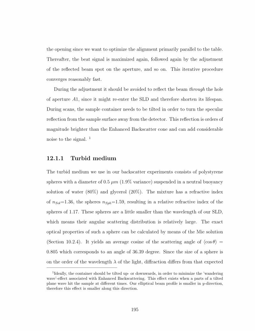
the opening since we want to optimize the alignment primarily parallel to the table.

Thereafter, the beat signal is maximized again, followed again by the adjustment

of the reflected beam spot on the aperture, and so on. This iterative procedure

converges reasonably fast.

During the adjustment it should be avoided to reflect the beam through the hole

of aperture A1, since it might re-enter the SLD and therefore shorten its lifespan.

During scans, the sample container needs to be tilted in order to turn the specular

reflection from the sample surface away from the detector. This reflection is orders of

magnitude brighter than the Enhanced Backscatter cone and can add considerable

noise to the signal. 1

12.1.1 Turbid medium

The turbid medium we use in our backscatter experiments consists of polystyrene

spheres with a diameter of 0.5 µm (1.9% variance) suspended in a neutral buoyancy

solution of water (80%) and glycerol (20%). The mixture has a refractive index

of nSol=1.36, the spheres nSph=1.59, resulting in a relative refractive index of the

spheres of 1.17. These spheres are a little smaller than the wavelength of our SLD,

which means their angular scattering distribution is relatively large. The exact

optical properties of such a sphere can be calculated by means of the Mie solution

(Section 10.2.4). It yields an average cosine of the scattering angle of 〈cos θ〉 =

0.805 which corresponds to an angle of 36.39 degree. Since the size of a sphere is

on the order of the wavelength λ of the light, diffraction differs from that expected

1Ideally, the container should be tilted up- or downwards, in order to minimize the ’wanderingwave’-effect associated with Enhanced Backscattering. This effect exists when a parts of a tiltedplane wave hit the sample at different times. Our elliptical beam profile is smaller in y-direction,therefore this effect is smaller along this direction.

195

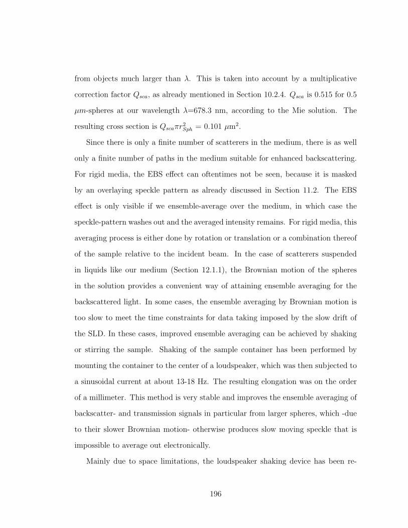
from objects much larger than λ. This is taken into account by a multiplicative

correction factor Qsca, as already mentioned in Section 10.2.4. Qsca is 0.515 for 0.5

µm-spheres at our wavelength λ=678.3 nm, according to the Mie solution. The

resulting cross section is Qscaπr2Sph = 0.101 µm2.

Since there is only a finite number of scatterers in the medium, there is as well

only a finite number of paths in the medium suitable for enhanced backscattering.

For rigid media, the EBS effect can oftentimes not be seen, because it is masked

by an overlaying speckle pattern as already discussed in Section 11.2. The EBS

effect is only visible if we ensemble-average over the medium, in which case the

speckle-pattern washes out and the averaged intensity remains. For rigid media, this

averaging process is either done by rotation or translation or a combination thereof

of the sample relative to the incident beam. In the case of scatterers suspended

in liquids like our medium (Section 12.1.1), the Brownian motion of the spheres

in the solution provides a convenient way of attaining ensemble averaging for the

backscattered light. In some cases, the ensemble averaging by Brownian motion is

too slow to meet the time constraints for data taking imposed by the slow drift of

the SLD. In these cases, improved ensemble averaging can be achieved by shaking

or stirring the sample. Shaking of the sample container has been performed by

mounting the container to the center of a loudspeaker, which was then subjected to

a sinusoidal current at about 13-18 Hz. The resulting elongation was on the order

of a millimeter. This method is very stable and improves the ensemble averaging of

backscatter- and transmission signals in particular from larger spheres, which -due

to their slower Brownian motion- otherwise produces slow moving speckle that is

impossible to average out electronically.

Mainly due to space limitations, the loudspeaker shaking device has been re-

196

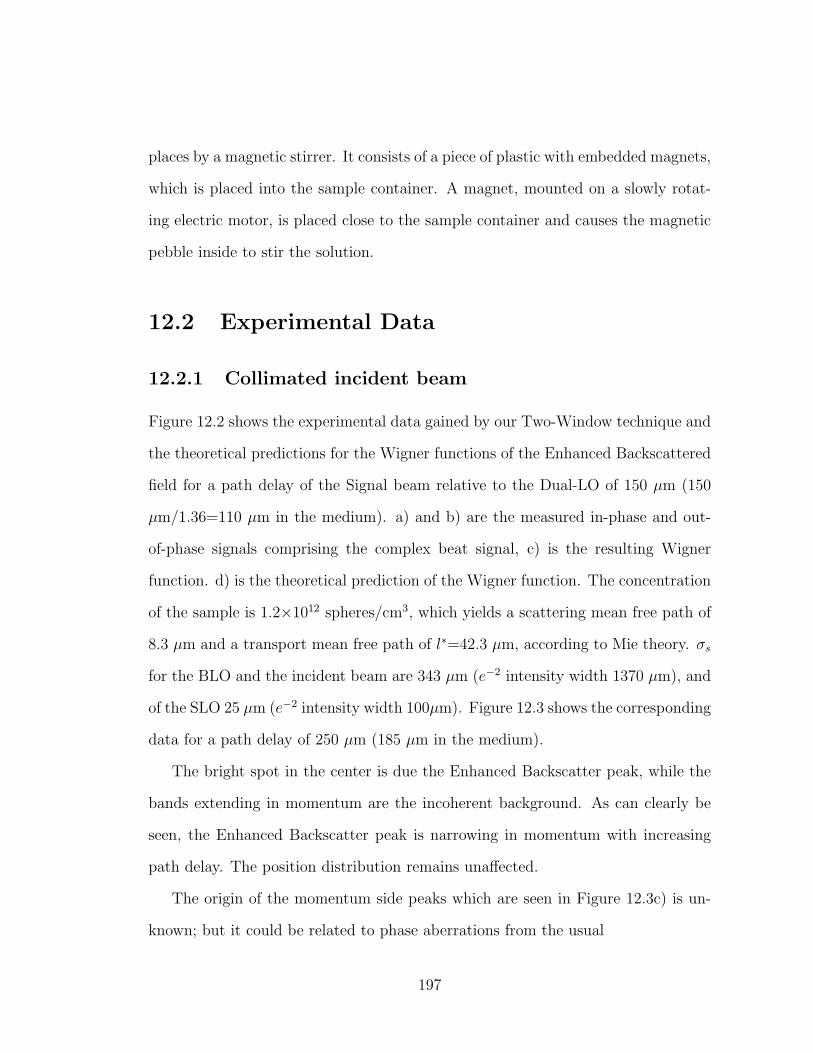
places by a magnetic stirrer. It consists of a piece of plastic with embedded magnets,

which is placed into the sample container. A magnet, mounted on a slowly rotat-

ing electric motor, is placed close to the sample container and causes the magnetic

pebble inside to stir the solution.

12.2 Experimental Data

12.2.1 Collimated incident beam

Figure 12.2 shows the experimental data gained by our Two-Window technique and

the theoretical predictions for the Wigner functions of the Enhanced Backscattered

field for a path delay of the Signal beam relative to the Dual-LO of 150 µm (150

µm/1.36=110 µm in the medium). a) and b) are the measured in-phase and out-

of-phase signals comprising the complex beat signal, c) is the resulting Wigner

function. d) is the theoretical prediction of the Wigner function. The concentration

of the sample is 1.2×1012 spheres/cm3, which yields a scattering mean free path of

8.3 µm and a transport mean free path of l∗=42.3 µm, according to Mie theory. σs

for the BLO and the incident beam are 343 µm (e−2 intensity width 1370 µm), and

of the SLO 25 µm (e−2 intensity width 100µm). Figure 12.3 shows the corresponding

data for a path delay of 250 µm (185 µm in the medium).

The bright spot in the center is due the Enhanced Backscatter peak, while the

bands extending in momentum are the incoherent background. As can clearly be

seen, the Enhanced Backscatter peak is narrowing in momentum with increasing

path delay. The position distribution remains unaffected.

The origin of the momentum side peaks which are seen in Figure 12.3c) is un-

known; but it could be related to phase aberrations from the usual

197

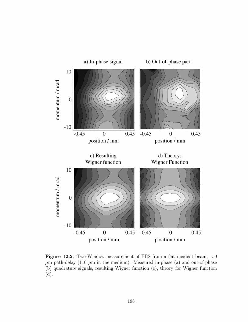
10

-10

0

mom

entu

m /

mra

d

position / mm0.45-0.45 0

a) In-phase signal b) Out-of-phase part

c) Resulting Wigner function

d) Theory: Wigner Function




mom

entu

m /

mra

d

10

-10

0

Figure 12.2: Two-Window measurement of EBS from a flat incident beam, 150µm path-delay (110 µm in the medium). Measured in-phase (a) and out-of-phase(b) quadrature signals, resulting Wigner function (c), theory for Wigner function(d).

198

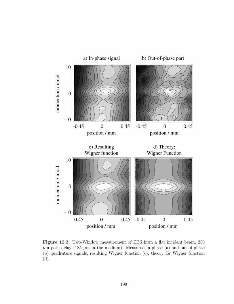
a) In-phase signal b) Out-of-phase part





c) Resulting Wigner function

d) Theory: Wigner Function

mom

entu

m /

mra

dm

omen

tum

/ m

rad

10

-10

0

10

-10

0

Figure 12.3: Two-Window measurement of EBS from a flat incident beam, 250µm path-delay (185 µm in the medium). Measured in-phase (a) and out-of-phase(b) quadrature signals, resulting Wigner function (c), theory for Wigner function(d).

199

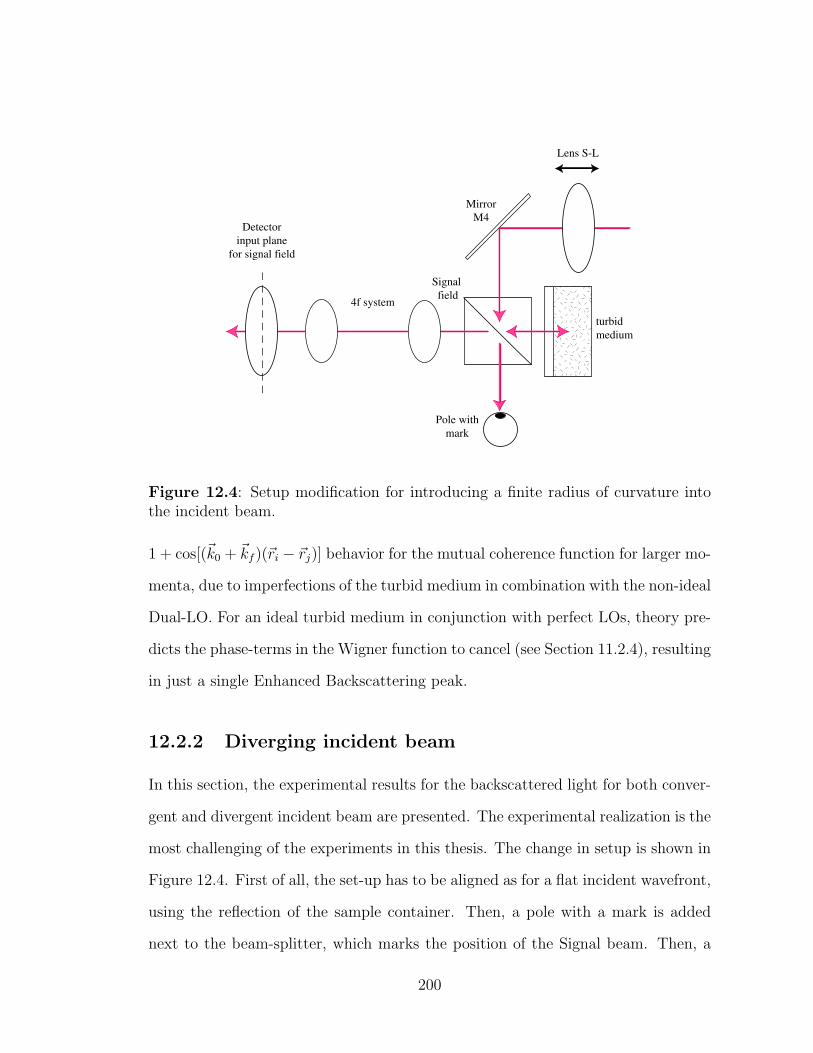
Signal field

4f system

Detector input plane

for signal field

turbid medium

Mirror M4

Pole with mark

Lens S-L

Figure 12.4: Setup modification for introducing a finite radius of curvature intothe incident beam.

1 + cos[(~k0 + ~kf )(~ri − ~rj)] behavior for the mutual coherence function for larger mo-

menta, due to imperfections of the turbid medium in combination with the non-ideal

Dual-LO. For an ideal turbid medium in conjunction with perfect LOs, theory pre-

dicts the phase-terms in the Wigner function to cancel (see Section 11.2.4), resulting

in just a single Enhanced Backscattering peak.

12.2.2 Diverging incident beam

In this section, the experimental results for the backscattered light for both conver-

gent and divergent incident beam are presented. The experimental realization is the

most challenging of the experiments in this thesis. The change in setup is shown in

Figure 12.4. First of all, the set-up has to be aligned as for a flat incident wavefront,

using the reflection of the sample container. Then, a pole with a mark is added

next to the beam-splitter, which marks the position of the Signal beam. Then, a

200

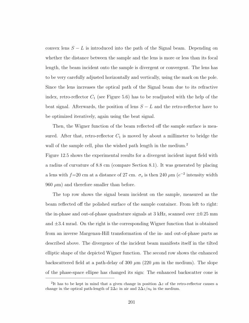
convex lens S − L is introduced into the path of the Signal beam. Depending on

whether the distance between the sample and the lens is more or less than its focal

length, the beam incident onto the sample is divergent or convergent. The lens has

to be very carefully adjusted horizontally and vertically, using the mark on the pole.

Since the lens increases the optical path of the Signal beam due to its refractive

index, retro-reflector C1 (see Figure 5.6) has to be readjusted with the help of the

beat signal. Afterwards, the position of lens S − L and the retro-reflector have to

be optimized iteratively, again using the beat signal.

Then, the Wigner function of the beam reflected off the sample surface is mea-

sured. After that, retro-reflector C1 is moved by about a millimeter to bridge the

wall of the sample cell, plus the wished path length in the medium.2

Figure 12.5 shows the experimental results for a divergent incident input field with

a radius of curvature of 8.8 cm (compare Section 8.1). It was generated by placing

a lens with f=20 cm at a distance of 27 cm. σs is then 240 µm (e−2 intensity width

960 µm) and therefore smaller than before.

The top row shows the signal beam incident on the sample, measured as the

beam reflected off the polished surface of the sample container. From left to right:

the in-phase and out-of-phase quadrature signals at 3 kHz, scanned over ±0.25 mm

and ±3.4 mrad. On the right is the corresponding Wigner function that is obtained

from an inverse Margenau-Hill transformation of the in- and out-of-phase parts as

described above. The divergence of the incident beam manifests itself in the tilted

elliptic shape of the depicted Wigner function. The second row shows the enhanced

backscattered field at a path-delay of 300 µm (220 µm in the medium). The slope

of the phase-space ellipse has changed its sign: The enhanced backscatter cone is

2It has to be kept in mind that a given change in position ∆z of the retro-reflector causes achange in the optical path-length of 2∆z in air and 2∆z/n0 in the medium.

201

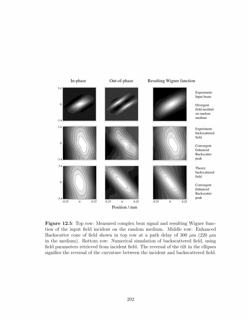
Position / mm-0.25 0.250 0.25-0.25 0 0.25-0.25 0

Mom

entu

m /

mra

d

3.4

3.4

-3.4

-3.4

In-phase Out-of-phase Resulting Wigner function

0

0

3.4

-3.4

0

Experiment: backscattered field Convergent Enhanced Backscatter peak

Experiment: Input beam Divergent field incident on random medium

Theory: backscattered field Convergent Enhanced Backscatter peak

Figure 12.5: Top row: Measured complex beat signal and resulting Wigner func-tion of the input field incident on the random medium. Middle row: EnhancedBackscatter cone of field shown in top row at a path delay of 300 µm (220 µmin the medium). Bottom row: Numerical simulation of backscattered field, usingfield parameters retrieved from incident field. The reversal of the tilt in the ellipsessignifies the reversal of the curvature between the incident and backscattered field.

202

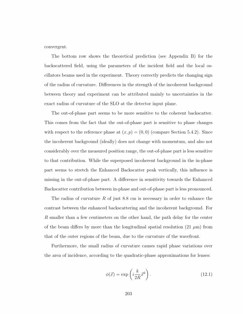
convergent.

The bottom row shows the theoretical prediction (see Appendix B) for the

backscattered field, using the parameters of the incident field and the local os-

cillators beams used in the experiment. Theory correctly predicts the changing sign

of the radius of curvature. Differences in the strength of the incoherent background

between theory and experiment can be attributed mainly to uncertainties in the

exact radius of curvature of the SLO at the detector input plane.

The out-of-phase part seems to be more sensitive to the coherent backscatter.

This comes from the fact that the out-of-phase part is sensitive to phase changes

with respect to the reference phase at (x, p) = (0, 0) (compare Section 5.4.2). Since

the incoherent background (ideally) does not change with momentum, and also not

considerably over the measured position range, the out-of-phase part is less sensitive

to that contribution. While the superposed incoherent background in the in-phase

part seems to stretch the Enhanced Backscatter peak vertically, this influence is

missing in the out-of-phase part. A difference in sensitivity towards the Enhanced

Backscatter contribution between in-phase and out-of-phase part is less pronounced.

The radius of curvature R of just 8.8 cm is necessary in order to enhance the

contrast between the enhanced backscattering and the incoherent background. For

R smaller than a few centimeters on the other hand, the path delay for the center

of the beam differs by more than the longitudinal spatial resolution (21 µm) from

that of the outer regions of the beam, due to the curvature of the wavefront.

Furthermore, the small radius of curvature causes rapid phase variations over

the area of incidence, according to the quadratic-phase approximations for lenses:

φ(~x) = exp

(i

k

2R~x2

). (12.1)

203

For R=10 cm, the center region of the beam, defined by phase deviations of not more

than ±π/2 from the center itself, is just 200 µm wide, followed by rapidly shrinking

concentric equal-phase regions. With increasing path delay, time-reversed paths

with starting points from bordering regions can interfere destructively, resulting in

what could be named ”Decreased Backscattering” or ”DBS”. The combination of

DBS and EBS leads to a wash-out of the Enhanced Backscatter signal when these

contributions cancel with constructively interfering time-reversed paths. We will

refer to this effect from now on as phase variation.

In addition to the phase variation, which can be completely attributed to the

properties of the Signal field, the imperfect Dual-LO introduces further problems:

The rapid phase changes outside the beams center region for small R’s in posi-

tion and momentum quickly drop below the resolution limit of the SLO and the

BLO. This leads to a smoothing and consequently a wash-out of these rapid oscil-

lations, which destroys the phase-information containing the radius of curvature of

the backscattered field.

Phase-variation and the finite resolution of the LOs are the reason why we get the

best results when we limit our range of measurement to the center of the Enhanced

Backscatter cone. If we include outer regions, the phase information washes out

and gives the EBS cone a flat appearance.

12.2.3 Converging incident beam

The experimental setup for a convergent incident beam is identical to the one for a

divergent incident beam, except that the distance between the sample and lens S−L

is now smaller than the focal length of S − L. Figure 12.7 shows the quadrature

signals of the complex beat signal for an incident beam of σs=310 µm and R=9 cm

204

-0.2 -0.20.2 0.2

3.3

-3.3

Position / mm0 0

0

Position / mm

mom

entu

m /

mra

d

-0.3 -0.30.3 0.30 0

5

-5

0

mom

entu

m /

mra

d

in-phase signal out-of-phase signal

incident field

backscattered field

a) b)

c) d)

Figure 12.6: In-phase- (a) and out-of-phase (b) quadrature signals for convergentincident beam. In-phase- (c) and out-of-phase (d) quadrature signals for EnhancedBackscatter cone at a path delay of 300 µm (220 µm in medium). A calculationof the Wigner function for the backscattered field is not possible due to the lowsignal-to-noise ratio. The incident field is of the same quality as that used in Fig-ure 12.5, but the scanning resolution is three times as small. The resolution for thebackscattered field is the same in both cases.

205

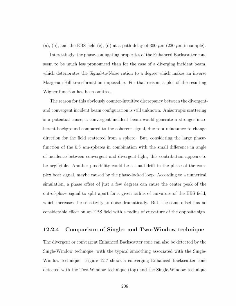
(a), (b), and the EBS field (c), (d) at a path-delay of 300 µm (220 µm in sample).

Interestingly, the phase-conjugating properties of the Enhanced Backscatter cone

seem to be much less pronounced than for the case of a diverging incident beam,

which deteriorates the Signal-to-Noise ration to a degree which makes an inverse

Margenau-Hill transformation impossible. For that reason, a plot of the resulting

Wigner function has been omitted.

The reason for this obviously counter-intuitive discrepancy between the divergent-

and convergent incident beam configuration is still unknown. Anisotropic scattering

is a potential cause; a convergent incident beam would generate a stronger inco-

herent background compared to the coherent signal, due to a reluctance to change

direction for the field scattered from a sphere. But, considering the large phase-

function of the 0.5 µm-spheres in combination with the small difference in angle

of incidence between convergent and divergent light, this contribution appears to

be negligible. Another possibility could be a small drift in the phase of the com-

plex beat signal, maybe caused by the phase-locked loop. According to a numerical

simulation, a phase offset of just a few degrees can cause the center peak of the

out-of-phase signal to split apart for a given radius of curvature of the EBS field,

which increases the sensitivity to noise dramatically. But, the same offset has no

considerable effect on an EBS field with a radius of curvature of the opposite sign.

12.2.4 Comparison of Single- and Two-Window technique

The divergent or convergent Enhanced Backscatter cone can also be detected by the

Single-Window technique, with the typical smoothing associated with the Single-

Window technique. Figure 12.7 shows a converging Enhanced Backscatter cone

detected with the Two-Window technique (top) and the Single-Window technique

206

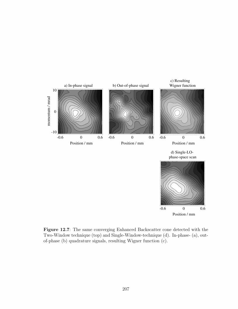
Position / mm-0.6 0.60 -0.6 0.60

-0.6 0.60

10

-10

0

mom

entu

m /

mra

d

Position / mm

Position / mm

a) In-phase signal b) Out-of-phase signal c) Resulting Wigner function

d) Single-LO- phase-space scan

-0.6 0.60Position / mm

Figure 12.7: The same converging Enhanced Backscatter cone detected with theTwo-Window technique (top) and Single-Window-technique (d). In-phase- (a), out-of-phase (b) quadrature signals, resulting Wigner function (c).

207

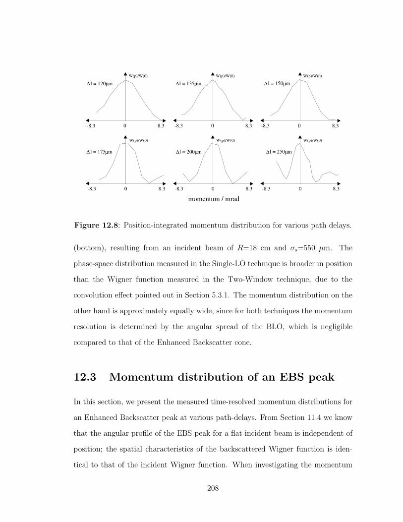
W(p)/W(0) W(p)/W(0) W(p)/W(0)

W(p)/W(0) W(p)/W(0) W(p)/W(0)

-8.3 8.30 -8.3 8.30 -8.3 8.30

-8.3 8.30 -8.3 8.30 -8.3 8.30

l = 120 mµ∆ l = 135 m∆ µ l = 150 m∆ µ

l = 175 m∆ µ l = 200 m∆ µ l = 250 m∆ µ

momentum / mrad

Figure 12.8: Position-integrated momentum distribution for various path delays.

(bottom), resulting from an incident beam of R=18 cm and σs=550 µm. The

phase-space distribution measured in the Single-LO technique is broader in position

than the Wigner function measured in the Two-Window technique, due to the

convolution effect pointed out in Section 5.3.1. The momentum distribution on the

other hand is approximately equally wide, since for both techniques the momentum

resolution is determined by the angular spread of the BLO, which is negligible

compared to that of the Enhanced Backscatter cone.

12.3 Momentum distribution of an EBS peak

In this section, we present the measured time-resolved momentum distributions for

an Enhanced Backscatter peak at various path-delays. From Section 11.4 we know

that the angular profile of the EBS peak for a flat incident beam is independent of

position; the spatial characteristics of the backscattered Wigner function is iden-

tical to that of the incident Wigner function. When investigating the momentum

208

distribution, we can therefore integrate the measured Wigner function over posi-

tion in order to improve ensemble averaging. Comparing the position-integrated

momentum distribution with that at the center of the EBS peak, it has been shown

that while the fluctuation are averaged out to a good degree, the shape of the EBS

peak remains unchanged.

Figure 12.8 shows the position-integrated momentum distributions for six dif-

ferent path delays ∆l between 120 and 250 µm. At 120 µm, the momentum dis-

tribution is Gaussian, because only the lowest scattering orders contribute. The

distribution at 135 µm is approximately triangular, which - according to the theory

to be discussed shortly - means that it contains contributions ranging from dual-

to about 135 µm/(n0l) ≈ 13 scatterers. According to theory, an EBS cone displays

the well-known triangular shape with a cusp only for perfectly coherent light and

absolutely loss-less scattering. The dual- and triple-scattering contributions which

are broad in momentum fill the wings of the triangle. Higher scattering orders are

narrow in momentum and shape the cusp. For ∆l=135 µm the EBS cone is triangu-

lar because the longitudinal coherence length of our SLD of 25 µm is large enough

to include both the scattering orders filling the wings and higher ones which fill the

cusp.

For larger path-delays at 150 µm and up, the path-delay resolution suppresses

the lowest scattering orders and the momentum distribution looses its wings. Also,

the EBS-side peaks, already seen in Figure 12.3c), become more prominent.

The various shapes seen can not be explained by the our current model which

employs the diffusion approximation and therefore a continuum of scatterers. In his

paper [62], Akkermans derives an expression for the angle-dependent intensity for

Enhanced Backscattering of a plane-wave incident on a semi-infinite medium, as a

209

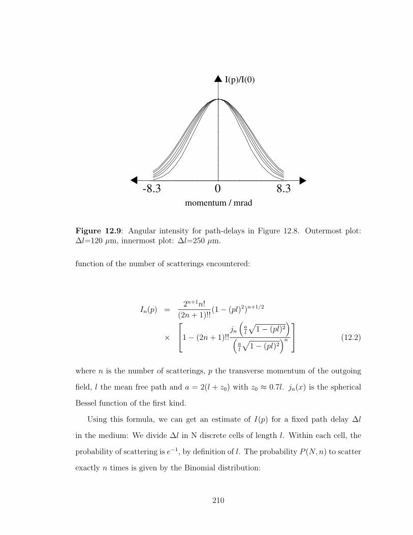
-8.3 8.30

I(p)/I(0)

momentum / mrad

Figure 12.9: Angular intensity for path-delays in Figure 12.8. Outermost plot:∆l=120 µm, innermost plot: ∆l=250 µm.

function of the number of scatterings encountered:

In(p) =2n+1n!

(2n + 1)!!(1− (pl)2)n+1/2

×1− (2n + 1)!!

jn

(al

√1− (pl)2

)(

al

√1− (pl)2

)n

(12.2)

where n is the number of scatterings, p the transverse momentum of the outgoing

field, l the mean free path and a = 2(l + z0) with z0 ≈ 0.7l. jn(x) is the spherical

Bessel function of the first kind.

Using this formula, we can get an estimate of I(p) for a fixed path delay ∆l

in the medium: We divide ∆l in N discrete cells of length l. Within each cell, the

probability of scattering is e−1, by definition of l. The probability P (N, n) to scatter

exactly n times is given by the Binomial distribution:

210

P (N,n) =

N

n

e−n(1− e)−(N−n). (12.3)

The intensity distribution for a fixed path delay in this model is then the sum over

the intensities involving n=2...N scattering events, each weighted by its probability

p(N,n):

I(N =∆l

l, p) =

N∑n=2

In(p) P (N, n). (12.4)

Figure 12.9 shows a plot of Eq. (12.3) for the values for the path-length in Fig-

ure 12.8. The outermost curve corresponds to ∆l=120µm; it becomes more narrow

with increasing ∆l, leading to the innermost curve for ∆l=250µm.

Theory predicts reasonably well the triangular shape observed for small path-

delays. The cone-width is also in good agreement with the experiment. For larger

path-delays, the experimentally observed width is much smaller than predicted,

maybe do the superposed oscillations of unknown origin which were discussed in

Section 12.2.3.

12.4 Discussion and Summary

The experimental results for a flat incident beam agree reasonably well with their

theoretical prediction. With increasing path-delay, the momentum distribution of

the EBS-peak narrows, while the position distribution remains unaffected. For a

divergent incident beam, the EBS-peak shows inversion of the radius of curvature.

Two incident wavelets can interfere even when they enter the medium at different

locations, which is different from a true phase-conjugating mirror. Therefore, and

211

because of the finite size and angular spread of the Dual LO, inversion of curvature

can be observed only close to the beam center, where the transverse phase of the

incident beam changes slowly.

Interestingly, an incident converging beam generates a far less pronounced in-

version than an incident divergent beam of the same absolute radius of curvature.

So far, no satisfying explanation for this asymmetry has been found. The finite

scattering angle of our polystyrene spheres could explain a higher concentration of

incoherent light for an incident converging beam, which would outshine the coherent

part. Although this assumption appears unlikely in light of the small differences

in incident angle with respect to the angular smear of the spheres, this theory

necessitates further study.

Position-integrated momentum distributions of the EBS peak display reason-

ably well the transition from Gaussian to triangular back to Gaussian shape, with

increasing path-delay, as predicted by our time-dependent extension of Akkerman’s

theory [62]. With increasing path-delay, the measured momentum-distribution be-

comes much narrower than predicted, displaying additional side-peaks closing in on

the main peak. The reason for those features, also seen in phase-space scans, is still

unknown, but can probably also be attributed to anisotropic scattering. To our

knowledge, there is no analytical method to calculate the shape of an EBS cone for

anisotropic scattering; therefore, future numerical simulations might be required.

212

Chapter 13

Transmission through randommedia

Measurement of the transmission of light through a medium is the simplest way to

determine parameters of the scatterers inside the medium. In the following, we will

look at the transmission through a turbid medium consisting of 10 µm polystyrene

spheres suspended in a neutral buoyancy solution. First, we will take measurements

with the Single-Window technique which does not allow for the immediate distinc-

tion between coherent and incoherent contributions, but which can be modelled

relatively easily, using a Monte-Carlo simulation I developed for two scatter events

or more.

In the second part we employ the Two-Window technique which directly allows

the detection of coherence but which poses a much greater challenge in modelling.

13.1 Experimental setup

The setup modifications for transmission measurements and its adjustment are rela-

tively simple compared to that for backscattering measurements. Figure 13.1 shows

those modifications close to the detection input plane. The Signal beam passes

through the sample cell containing the turbid medium. The surface of the turbid

213

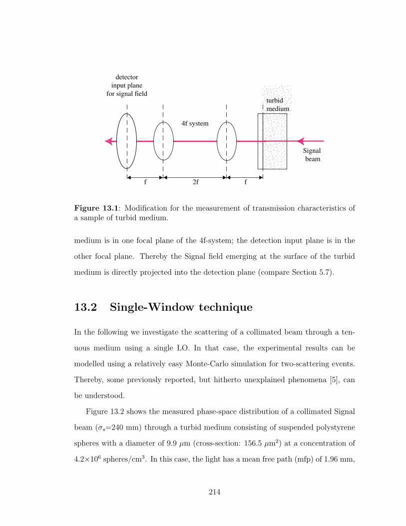
Signal beam

4f system

detector input plane

for signal fieldturbid medium

f f2f

Figure 13.1: Modification for the measurement of transmission characteristics ofa sample of turbid medium.

medium is in one focal plane of the 4f-system; the detection input plane is in the

other focal plane. Thereby the Signal field emerging at the surface of the turbid

medium is directly projected into the detection plane (compare Section 5.7).

13.2 Single-Window technique

In the following we investigate the scattering of a collimated beam through a ten-

uous medium using a single LO. In that case, the experimental results can be

modelled using a relatively easy Monte-Carlo simulation for two-scattering events.

Thereby, some previously reported, but hitherto unexplained phenomena [5], can

be understood.

Figure 13.2 shows the measured phase-space distribution of a collimated Signal

beam (σs=240 mm) through a turbid medium consisting of suspended polystyrene

spheres with a diameter of 9.9 µm (cross-section: 156.5 µm2) at a concentration of

4.2×106 spheres/cm3. In this case, the light has a mean free path (mfp) of 1.96 mm,

214

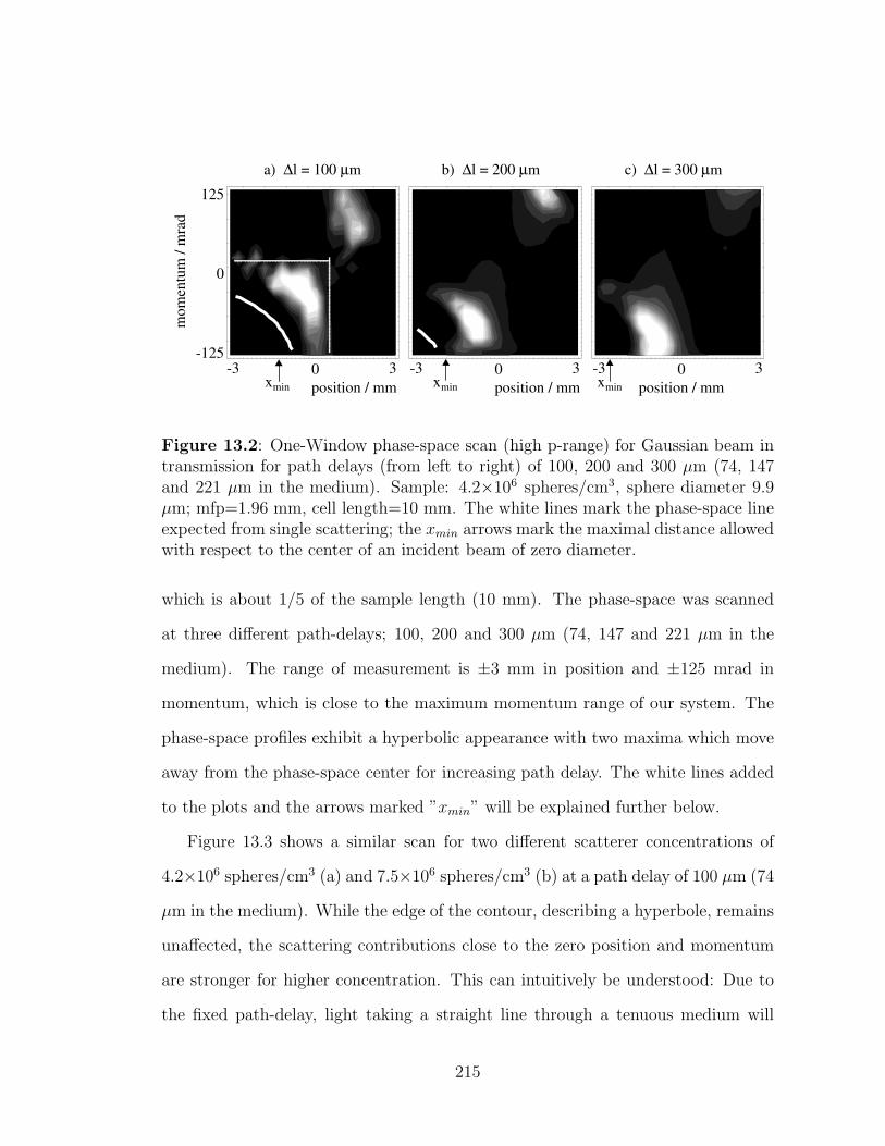
position / mm-3 30 -3 30 -3 30


mom

entu

m /

mra

d

-125

125

0

a) ∆l = 100 µm c) ∆l = 300 µm b) ∆l = 200 µm

xmin xminxmin

Figure 13.2: One-Window phase-space scan (high p-range) for Gaussian beam intransmission for path delays (from left to right) of 100, 200 and 300 µm (74, 147and 221 µm in the medium). Sample: 4.2×106 spheres/cm3, sphere diameter 9.9µm; mfp=1.96 mm, cell length=10 mm. The white lines mark the phase-space lineexpected from single scattering; the xmin arrows mark the maximal distance allowedwith respect to the center of an incident beam of zero diameter.

which is about 1/5 of the sample length (10 mm). The phase-space was scanned

at three different path-delays; 100, 200 and 300 µm (74, 147 and 221 µm in the

medium). The range of measurement is ±3 mm in position and ±125 mrad in

momentum, which is close to the maximum momentum range of our system. The

phase-space profiles exhibit a hyperbolic appearance with two maxima which move

away from the phase-space center for increasing path delay. The white lines added

to the plots and the arrows marked ”xmin” will be explained further below.

Figure 13.3 shows a similar scan for two different scatterer concentrations of

4.2×106 spheres/cm3 (a) and 7.5×106 spheres/cm3 (b) at a path delay of 100 µm (74

µm in the medium). While the edge of the contour, describing a hyperbole, remains

unaffected, the scattering contributions close to the zero position and momentum

are stronger for higher concentration. This can intuitively be understood: Due to

the fixed path-delay, light taking a straight line through a tenuous medium will

215

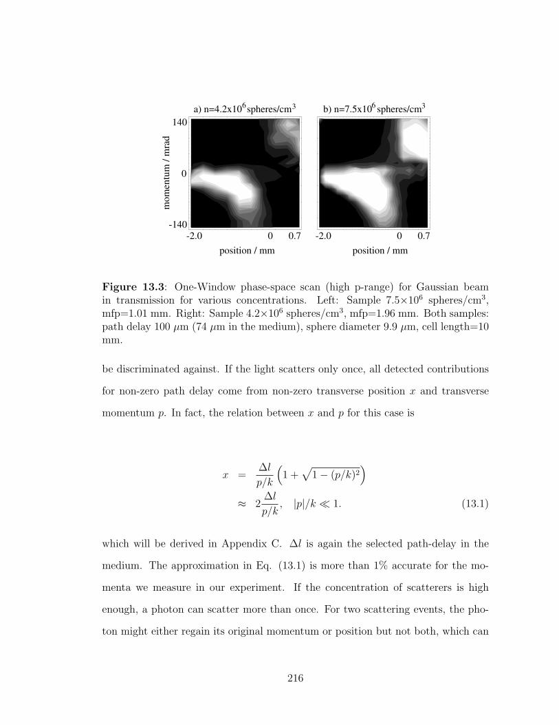
position / mm

mom

entu

m /

mra

d

-2.0 0.70 -2.0 0.70-140

140

0

position / mm

b) n=7.5x10 spheres/cm 3 6 a) n=4.2x10 spheres/cm 3 6

Figure 13.3: One-Window phase-space scan (high p-range) for Gaussian beamin transmission for various concentrations. Left: Sample 7.5×106 spheres/cm3,mfp=1.01 mm. Right: Sample 4.2×106 spheres/cm3, mfp=1.96 mm. Both samples:path delay 100 µm (74 µm in the medium), sphere diameter 9.9 µm, cell length=10mm.

be discriminated against. If the light scatters only once, all detected contributions

for non-zero path delay come from non-zero transverse position x and transverse

momentum p. In fact, the relation between x and p for this case is

x =∆l

p/k

(1 +

√1− (p/k)2

)

≈ 2∆l

p/k, |p|/k ¿ 1. (13.1)

which will be derived in Appendix C. ∆l is again the selected path-delay in the

medium. The approximation in Eq. (13.1) is more than 1% accurate for the mo-

menta we measure in our experiment. If the concentration of scatterers is high

enough, a photon can scatter more than once. For two scattering events, the pho-

ton might either regain its original momentum or position but not both, which can

216

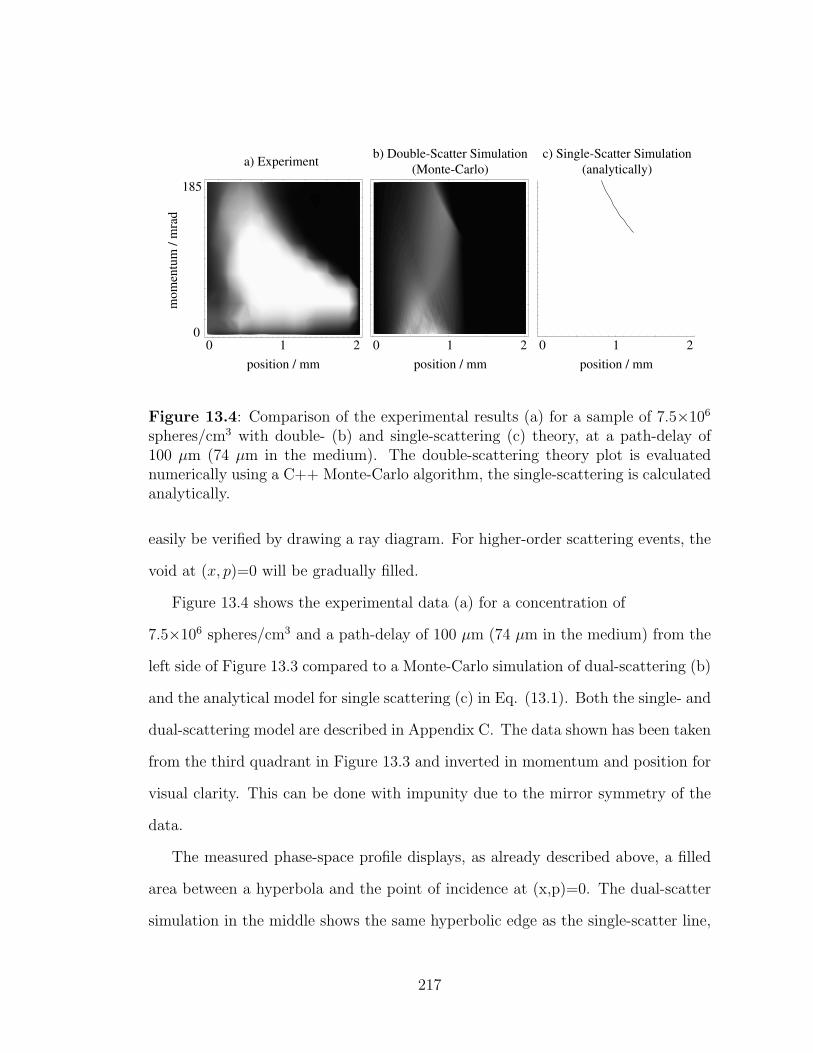
a) Experiment b) Double-Scatter Simulation (Monte-Carlo)

c) Single-Scatter Simulation (analytically)

0

185

0 21 0 21 0 21position / mm

mom

entu

m /

mra

d


Figure 13.4: Comparison of the experimental results (a) for a sample of 7.5×106

spheres/cm3 with double- (b) and single-scattering (c) theory, at a path-delay of100 µm (74 µm in the medium). The double-scattering theory plot is evaluatednumerically using a C++ Monte-Carlo algorithm, the single-scattering is calculatedanalytically.

easily be verified by drawing a ray diagram. For higher-order scattering events, the

void at (x, p)=0 will be gradually filled.

Figure 13.4 shows the experimental data (a) for a concentration of

7.5×106 spheres/cm3 and a path-delay of 100 µm (74 µm in the medium) from the

left side of Figure 13.3 compared to a Monte-Carlo simulation of dual-scattering (b)

and the analytical model for single scattering (c) in Eq. (13.1). Both the single- and

dual-scattering model are described in Appendix C. The data shown has been taken

from the third quadrant in Figure 13.3 and inverted in momentum and position for

visual clarity. This can be done with impunity due to the mirror symmetry of the

data.

The measured phase-space profile displays, as already described above, a filled

area between a hyperbola and the point of incidence at (x,p)=0. The dual-scatter

simulation in the middle shows the same hyperbolic edge as the single-scatter line,

217

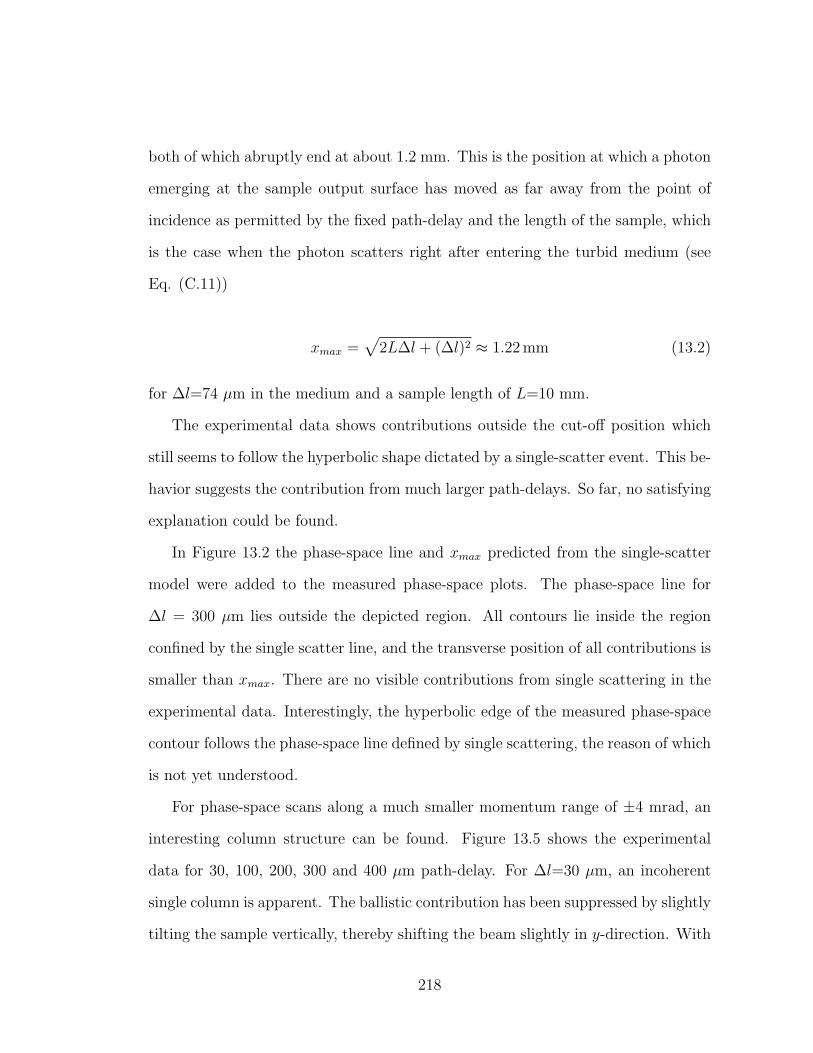
both of which abruptly end at about 1.2 mm. This is the position at which a photon

emerging at the sample output surface has moved as far away from the point of

incidence as permitted by the fixed path-delay and the length of the sample, which

is the case when the photon scatters right after entering the turbid medium (see

Eq. (C.11))

xmax =√

2L∆l + (∆l)2 ≈ 1.22 mm (13.2)

for ∆l=74 µm in the medium and a sample length of L=10 mm.

The experimental data shows contributions outside the cut-off position which

still seems to follow the hyperbolic shape dictated by a single-scatter event. This be-

havior suggests the contribution from much larger path-delays. So far, no satisfying

explanation could be found.

In Figure 13.2 the phase-space line and xmax predicted from the single-scatter

model were added to the measured phase-space plots. The phase-space line for

∆l = 300 µm lies outside the depicted region. All contours lie inside the region

confined by the single scatter line, and the transverse position of all contributions is

smaller than xmax. There are no visible contributions from single scattering in the

experimental data. Interestingly, the hyperbolic edge of the measured phase-space

contour follows the phase-space line defined by single scattering, the reason of which

is not yet understood.

For phase-space scans along a much smaller momentum range of ±4 mrad, an

interesting column structure can be found. Figure 13.5 shows the experimental

data for 30, 100, 200, 300 and 400 µm path-delay. For ∆l=30 µm, an incoherent

single column is apparent. The ballistic contribution has been suppressed by slightly

tilting the sample vertically, thereby shifting the beam slightly in y-direction. With

218

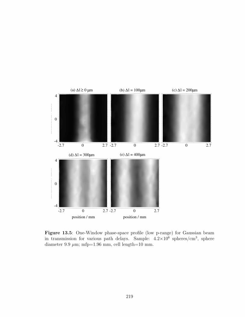
-2.7 2.70

-2.7 2.70

-2.7 2.70

-2.7 2.70 -2.7 2.70

position / mmposition / mm

-4

4

0

mom

entu

m /

mra

dm

omen

tum

/ m

rad

-4

4

0

l = 100 mµ∆l 0 mµ∆ >∼ l = 200 mµ∆

l = 300 mµ∆ l = 400 mµ∆

(a) (b) (c)

(d) (e)

Figure 13.5: One-Window phase-space profile (low p-range) for Gaussian beamin transmission for various path delays. Sample: 4.2×106 spheres/cm3, spherediameter 9.9 µm; mfp=1.96 mm, cell length=10 mm.

219

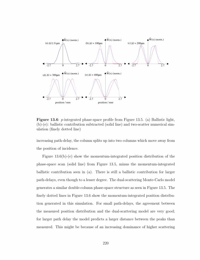
-2.7 2.70 -2.7 2.70 -2.7 2.70

-2.7 2.70 -2.7 2.70

l = 100 mµ∆l 0 mµ∆ >∼ l = 200 mµ∆

l = 300 mµ∆ l = 400 mµ∆

position / mmposition / mm

W(x) (norm.)~

W(x) (norm.)~ W(x) (norm.)

~

W(x) (norm.)~

W(x) (norm.)~

(a) (b) (c)

(d) (e)

Figure 13.6: p-integrated phase-space profile from Figure 13.5. (a) Ballistic light,(b)-(e): ballistic contribution subtracted (solid line) and two-scatter numerical sim-ulation (finely dotted line)

increasing path-delay, the column splits up into two columns which move away from

the position of incidence.

Figure 13.6(b)-(e) show the momentum-integrated position distribution of the

phase-space scan (solid line) from Figure 13.5, minus the momentum-integrated

ballistic contribution seen in (a). There is still a ballistic contribution for larger

path-delays, even though to a lesser degree. The dual-scattering Monte-Carlo model

generates a similar double-column phase-space structure as seen in Figure 13.5. The

finely dotted lines in Figure 13.6 show the momentum-integrated position distribu-

tion generated in this simulation. For small path-delays, the agreement between

the measured position distribution and the dual-scattering model are very good;

for larger path delay the model predicts a larger distance between the peaks than

measured. This might be because of an increasing dominance of higher scattering

220

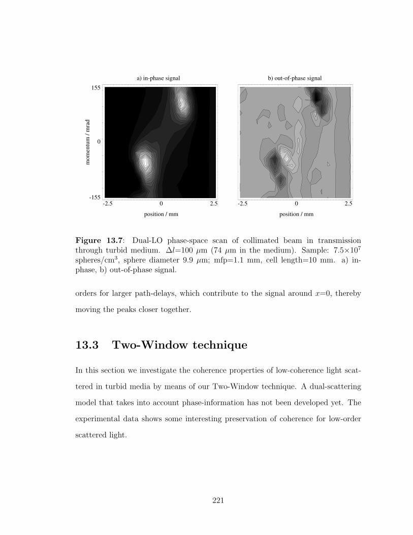
155

-155-2.5 -2.52.5 2.5

0

0 0


mom

entu

m /

mra

da) in-phase signal b) out-of-phase signal

Figure 13.7: Dual-LO phase-space scan of collimated beam in transmissionthrough turbid medium. ∆l=100 µm (74 µm in the medium). Sample: 7.5×107

spheres/cm3, sphere diameter 9.9 µm; mfp=1.1 mm, cell length=10 mm. a) in-phase, b) out-of-phase signal.

orders for larger path-delays, which contribute to the signal around x=0, thereby

moving the peaks closer together.

13.3 Two-Window technique

In this section we investigate the coherence properties of low-coherence light scat-

tered in turbid media by means of our Two-Window technique. A dual-scattering

model that takes into account phase-information has not been developed yet. The

experimental data shows some interesting preservation of coherence for low-order

scattered light.

221

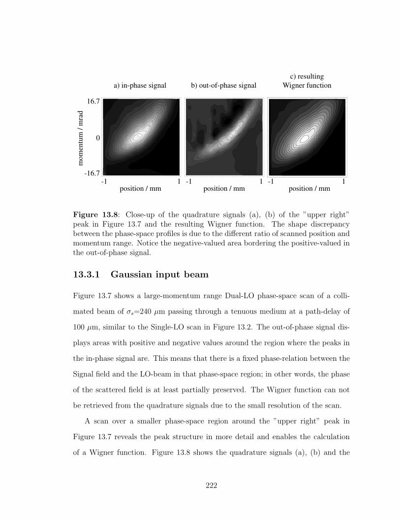
a) in-phase signal b) out-of-phase signalc) resulting

Wigner function

position / mm position / mm position / mm

mom

entu

m /

mra

d

-1 -1 -11 1 1

16.7

-16.7

0

Figure 13.8: Close-up of the quadrature signals (a), (b) of the ”upper right”peak in Figure 13.7 and the resulting Wigner function. The shape discrepancybetween the phase-space profiles is due to the different ratio of scanned position andmomentum range. Notice the negative-valued area bordering the positive-valued inthe out-of-phase signal.

13.3.1 Gaussian input beam

Figure 13.7 shows a large-momentum range Dual-LO phase-space scan of a colli-

mated beam of σs=240 µm passing through a tenuous medium at a path-delay of

100 µm, similar to the Single-LO scan in Figure 13.2. The out-of-phase signal dis-

plays areas with positive and negative values around the region where the peaks in

the in-phase signal are. This means that there is a fixed phase-relation between the

Signal field and the LO-beam in that phase-space region; in other words, the phase

of the scattered field is at least partially preserved. The Wigner function can not

be retrieved from the quadrature signals due to the small resolution of the scan.

A scan over a smaller phase-space region around the ”upper right” peak in

Figure 13.7 reveals the peak structure in more detail and enables the calculation

of a Wigner function. Figure 13.8 shows the quadrature signals (a), (b) and the

222

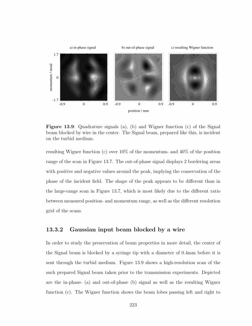
a) in-phase signal b) out-of-phase signal c) resulting Wigner function

-0.9 0.90 -0.9 0.90 -0.9 0.90

1.7

-1.7

0

position / mm

mom

entu

m /

mra

d

Figure 13.9: Quadrature signals (a), (b) and Wigner function (c) of the Signalbeam blocked by wire in the center. The Signal beam, prepared like this, is incidenton the turbid medium.

resulting Wigner function (c) over 10% of the momentum- and 40% of the position

range of the scan in Figure 13.7. The out-of-phase signal displays 2 bordering areas

with positive and negative values around the peak, implying the conservation of the

phase of the incident field. The shape of the peak appears to be different than in

the large-range scan in Figure 13.7, which is most likely due to the different ratio

between measured position- and momentum range, as well as the different resolution

grid of the scans.

13.3.2 Gaussian input beam blocked by a wire

In order to study the preservation of beam properties in more detail, the center of

the Signal beam is blocked by a syringe tip with a diameter of 0.4mm before it is

sent through the turbid medium. Figure 13.9 shows a high-resolution scan of the

such prepared Signal beam taken prior to the transmission experiments. Depicted

are the in-phase- (a) and out-of-phase (b) signal as well as the resulting Wigner

function (c). The Wigner function shows the beam lobes passing left and right to

223

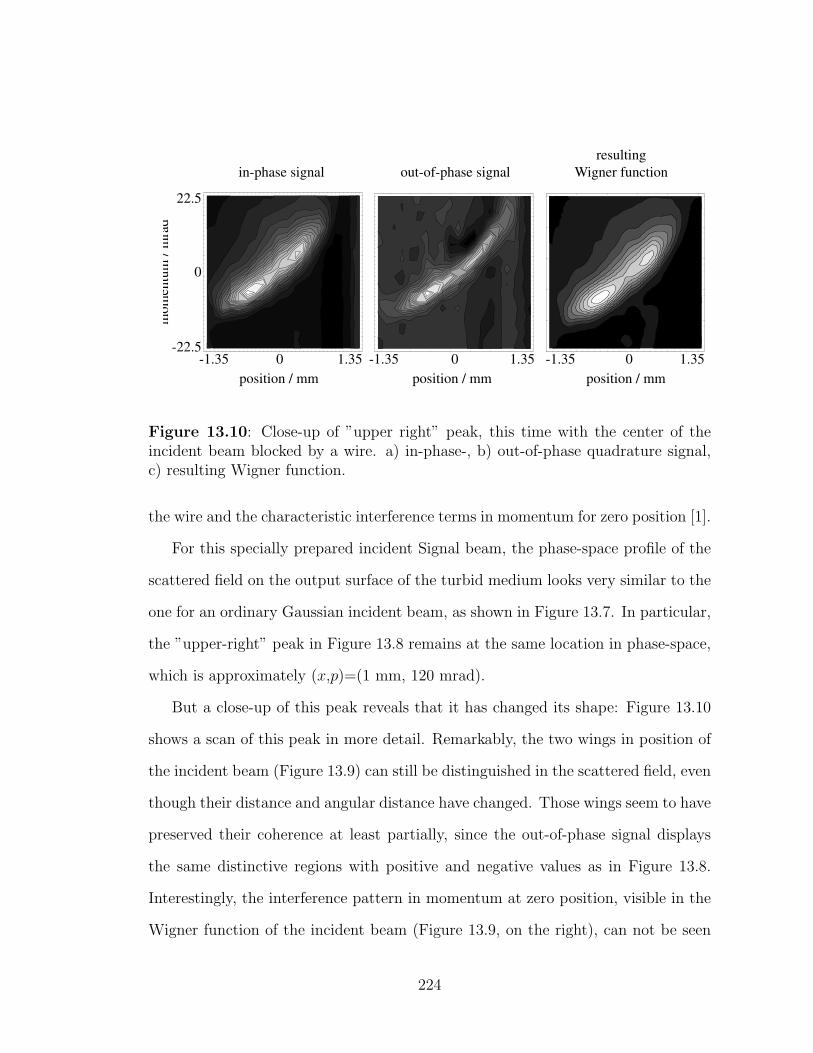
in-phase signal out-of-phase signal resulting

Wigner function

position / mm position / mm position / mm

mom

entu

m /

mra

d

22.5

-22.5 -1.35 -1.35 -1.35 1.35 1.35 1.35 0 0 0

0

Figure 13.10: Close-up of ”upper right” peak, this time with the center of theincident beam blocked by a wire. a) in-phase-, b) out-of-phase quadrature signal,c) resulting Wigner function.

the wire and the characteristic interference terms in momentum for zero position [1].

For this specially prepared incident Signal beam, the phase-space profile of the

scattered field on the output surface of the turbid medium looks very similar to the

one for an ordinary Gaussian incident beam, as shown in Figure 13.7. In particular,

the ”upper-right” peak in Figure 13.8 remains at the same location in phase-space,

which is approximately (x,p)=(1 mm, 120 mrad).

But a close-up of this peak reveals that it has changed its shape: Figure 13.10

shows a scan of this peak in more detail. Remarkably, the two wings in position of

the incident beam (Figure 13.9) can still be distinguished in the scattered field, even

though their distance and angular distance have changed. Those wings seem to have

preserved their coherence at least partially, since the out-of-phase signal displays

the same distinctive regions with positive and negative values as in Figure 13.8.

Interestingly, the interference pattern in momentum at zero position, visible in the

Wigner function of the incident beam (Figure 13.9, on the right), can not be seen

224

for the scattered field, which could be due to a decrease in coherence.

13.4 Discussion and Summary

Both the Single- and Two-Window technique enable the characterization of the

propagation of partially coherent light in turbid media. We have examined the path-

length dependent locations in phase-space of two peaks resulting from low-order

scattering (Section 13.2). We also demonstrated the greater contribution of higher-

order scattering to the (smoothed) Wigner function in the phase-space region close

to the incident beam. The borders of the (smoothed) Wigner function are defined

by a hyperbola, independent on the number of scatterers involved, which agrees

with predictions by an analytical calculation of time-resolved single-scattering as

well as a Monte-Carlo simulation of time-resolved double-scattering.

For small transverse momenta the smoothed Wigner function consists of two

incoherent, spatially confined structures, which move apart with increasing path

delay. This phenomenon, which is due to the finite size of the incident beam, can

not be explained by the single-scattering theory, which predicts two peaks with

momenta 2 orders of magnitude larger than the ones contained in the phase-space

measured in this scan. The double-scattering theory describes the location of the

columns increasingly well for larger path-delays. The main contribution close to the

location of the incident beam (x=0) for small path-delays can not be explained by

either theory and is most likely due to multiple, almost forward scattered light.

The two phase-space peaks observed as a result of low-order scattering in Sec-

tion 13.2 partially conserve the coherence of the incident field, as measurements

with the Two-Window technique confirm (Section 13.3). Even the spatial profile of

the incident field is to a good degree conserved, as measurements with a specially

225

prepared incident beam, a Gaussian beam whose center is blocked by a wire, show.

226

Chapter 14

Summary

In this dissertation, I presented a new Two-Window Heterodyne method which

allows the direct measurement of the Wigner function of a light field. Wigner

functions present a convenient way to fully characterize light fields up to their first-

order-coherence properties; they simultaneously describe the transverse position and

momentum of a light field while preserving all phase and amplitude information of

the field. Wigner functions obey rigorous transport equations and are a convenient

way to describe the propagation of fields. Our new technique also allows us for the

first time to directly distinguish between coherent and incoherent parts of the field

by means of the out-of-phase quadrature signal, which, together with the in-phase

signal, comprises the measured complex beat signal. Due to the low-coherence

light we employ, the measurements are time-resolved, which allows us to exclusively

detect photons that have travelled a given path length in the medium under investi-

gation. This time-resolution in combination with the combination of high position-

and momentum resolution of this method will enable new ways of characterizing

light fields scattered from, for example, biological samples and thereby refine the

determination of their structural properties.

The Two-Window technique is based on the heterodyne detection of the two

beat notes resulting from the superposition of the measured signal field and a so-

227

called Dual-LO, which consists of a superposed, phase-coupled set of a focused LO

(SLO) and a collimated beam (BLO). The focused beam determines the spatial x

resolution and the collimated beam the momental p resolution. This is different

from the One-Window method we formerly employed where we used a single LO

which determined the resolution of both x and p, leading to a trade-off between

both resolutions. In that case, only smoothed Wigner functions can be measured,

which are the convolution between the true Wigner function of the Signal field and

the spatial and momental profile of the LO. The Two-Window technique on the

other hand allows the measurement of true Wigner functions, given that the SLO is

sufficiently focused and the BLO sufficiently collimated. The Wigner function can

be retrieved from the measured complex beat signal by an inverse Margenau-Hill

transformation.

By varying the relative path-delay between Signal beam and Dual-LO, photons

that have travelled a given path in the medium can be detected exclusively. Since

the measured beat signal is proportional to the square root of the power of the

signal field rather than the power itself, as in direct intensity measurements, the

dynamic range is very high: for a Dual-LO on the order of a milliwatt, signal fields

of less than a femtowatt can be detected. The dynamic range is 130 dB.

The power of this method is first demonstrated in the determination of basic

field parameters of a Gaussian Signal beam in Chapter 7 and Chapter 8, where we

show how to retrieve its beam size, transverse coherence and radius of curvature.

This method is also applicable to more complicated fields. In Chapter 9 we exam-

ine the longitudinal properties of the Signal field, which are related to its optical

spectrum. The broad spectrum of the superluminescent diode we use as our light

source is responsible for the short longitudinal coherence length of 25 µm that can

228

be experimentally verified straightforwardly. The origin of other features seen in

the longitudinal scans, such as a phase-gradient, are still subject to debate. For

a laser diode with several transverse modes, this technique offers the possibility of

measuring the frequency-offset from the center-frequency as well as the spatial and

momental profile of those modes.

The second part of this thesis examines the propagation of a partially coherent

field in turbid media. Our turbid medium consists of polystyrene spheres suspended

in a neutral-buoyancy glycerol-water solution. We use two different sphere diame-

ters; 0.5 µm, which is close to the wavelength of our light (678.3 nm) and therefore

provides a broad angular scattering distribution, and 10 µm, where the field scatters

within a very narrow forward-cone.

In Chapter 11 and Chapter 12 we investigate the Enhanced Backscattering effect

by measuring the Wigner function of a field scattered from a relatively dense turbid

medium with highly scattering spheres (0.5 µm diameter). Enhanced Backscattering

describes the phenomenon of constructive interference of two counter-propagating

wavelets scattered in a turbid medium by the same sequence of scatterers. This

leads to twice the intensity of the backscattered field opposite to the direction of

incidence compared to other directions.

First, we shine a collimated beam onto the medium and observe how the En-

hanced Backscattered peak becomes more narrow with increasing path-delay. We

study the momentum distribution in more detail by position-integrating the backscat-

tered field. The change in shape of the momentum distribution allows us to estimate

the number of scatterers in a typical sequence.

For the first time we directly show the phase-conjugating properties of turbid

media by having a divergent or convergent Signal beam incident onto the medium

229

and observe the change of sign of the radius of curvature of the Enhanced Backscat-

tered field. This works best with a divergent incident beam, where the Enhanced

Backscattered cone is convergent. The reason for the discrepancy between conver-

gent and divergent incident beam configuration is still unknown, yet several possible

explanations are discussed.

We can explain the general behavior of the Enhanced Backscattered field, such

as the ratio of coherently and incoherently backscattered light, the narrowing of the

momentum distribution for increasing path-delay, and the inversion of the radius

of curvature for incident light with a curved wavefront, by a theory in which the

propagation of the Wigner function in the medium obeys the diffusion equation.

We study the time-resolved propagation of partially coherent light through tur-

bid media of various concentrations in the transmission regime in Chapter 13. For

tenuous to intermediate scatterer concentrations we observe two peaks in phase-

space probably as the result of low-order scattering and the path-length constraint

imposed by the time-resolution of our technique. We demonstrate how their rela-

tive distance becomes bigger with increasing path-delay. The Wigner function of

the transmitted field for a given path-delay is confined in phase-space by a hyper-

bolic edge which comes from single-scatter events. The contributions close to the

region in phase-space where the incident beam is located are relatively small for

tenuous media, but become stronger with increasing concentration of scatterers.

This region displays two column-shaped incoherent structures which are due to the

finite size in phase-space of the incident beam and which move apart with increas-

ing path-delay. While the explanation for the short distance between the columns

for small path-delays probably lies in higher-order scattering, for larger path-delay

a two-scattering Monte-Carlo algorithm I developed models the distance of the

230

columns correctly. This suggests that for large path-delays, the path-length restric-

tion, probably in combination with the narrow phase function of the 10 µm spheres,

increases the contributions from scattering paths which follow those expected for

double-scattering. Additional experiments with smaller scatterers could probably

illuminate this question.

Measurements of the transmitted time-resolved Wigner function by means of

the Two-Window technique reveal coherence of low-order scattered light, which

manifests itself in a slowly changing phase distribution around the two peaks in

phase-space which result from low-order scattering. Even spatial properties of the

incident beams are conserved: When we block the center of the incident beam by a

wire, the two lobes passing to the right and left of the wire show up in each of the

two peaks. While the peaks still display coherence, they do so to a lesser degree

than the incident field.

While many aspects of the propagation of partially coherent light in turbid media

are understood, there are still many open questions. For example, the Enhanced

Backscattered fields measured in our experiment averages over areas several times

as large as the coherence area of the EBS cone, because of the finite size of our

SLO. The coherence area of an EBS cone has a diameter the typical size of the

diffusion path√

Dt = 13l∗∆l/n0, where D is the diffusion constant of the intensity

in the medium, t the time after entering the medium, l∗ is the transport mean

free path, ∆l the length of the path in the medium and n0 the refractive index of

the solution between the scatterers. In future experiments, we plan to resolve the

Wigner function within a single coherence area by using a magnifying 4f-system

to gain a deeper understanding of the properties of the EBS field. This might

also clarify the origin of the momentum-side peaks of the EBS cone as seen in

231

Figure 12.3, for example. Those peaks could hint towards aberrations from the

diffusion equation usually used to model Enhanced Backscattering.

232

Appendix A

Circuit diagrams

A.1 Temperature control

Figure A.1 shows the temperature control for the SLD. It measures the temperature

close to the SLD by means of a temperature-dependent resistor (NTC, negative

temperature coefficient), which is mounted on top of the SLD in its casing. If the

temperature deviates from a selected value, the temperature control sends a positive

or negative current to a Peltier element which is mounted next to the SLD in its

casing, until the temperature difference drops below a certain value.

The centerpiece of the temperature control consists of a Wien bridge, with the

NTC being one of its four resistors. The reference resistance is selected by an array

of resistors and a potentiometer as shown in Figure A.2. When the resistance of

the NTC falls below or rises above that reference value, the Wien bridge delivers a

positive or negative voltage, which is amplified in comparer IC1. A low-pass filter

at its input slows down its operation to avoid oscillations. Operational amplifier

IC2 buffers the voltage for an analog display. Switch S permits switching between

two different resolutions of the voltage-proportional temperature inside the SLD

casing. Operational amplifier IC3 amplifies the Wien bridge voltage and controls

the power amplifier. It also acts as an integrator, with the RC-(glied) in its feedback

233

+

_

+

_

+

_

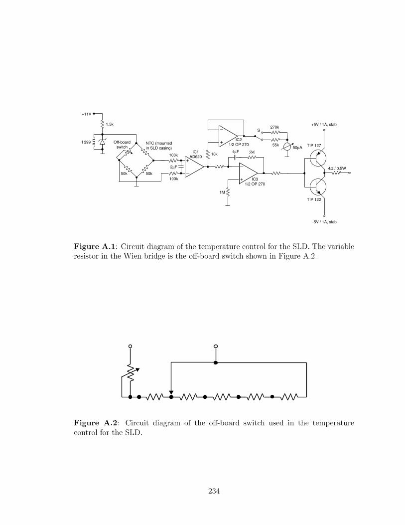
1.5k

LM 399 NTC (mounted in SLD casing)

50k 50k

100k

100k

2µF

10k

270k

55k50µA

TIP 122

TIP 127

4Ω / 0.5W

IC3 1/2 OP 270

IC2 1/2 OP 270

4µF 5Μ

+5V / 1A, stab.

-5V / 1A, stab.

1M

Off-board switch

+11V

IC1 AD620

S

Figure A.1: Circuit diagram of the temperature control for the SLD. The variableresistor in the Wien bridge is the off-board switch shown in Figure A.2.

Figure A.2: Circuit diagram of the off-board switch used in the temperaturecontrol for the SLD.

234

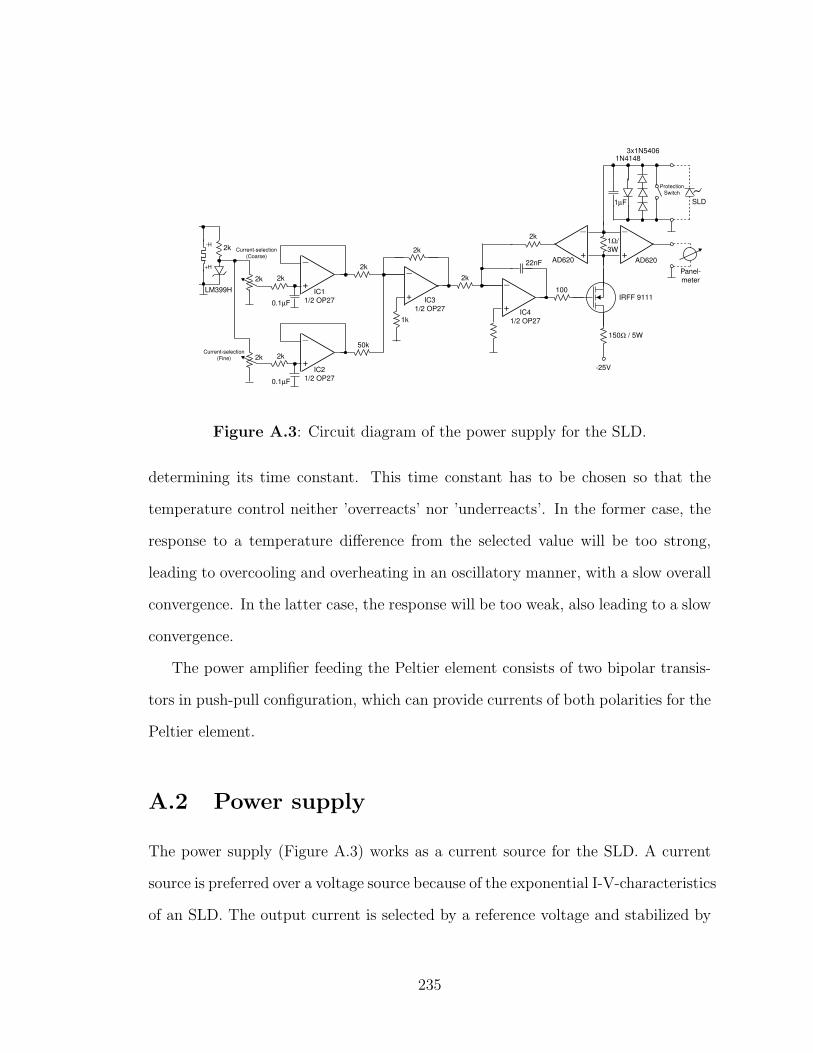
-11V

+

_

+

_

+

_

+

_

+

_

+

_

100µF

LM399H

2k

2k

2k

2k

2k

0.1µF

0.1µF

IC1 1/2 OP27

IC2 1/2 OP27

2k

50k

2k

1k

IC3 1/2 OP27

2k

IC4 1/2 OP27

22nF

100

AD620

2k

1µF

1N41483x1N5406

-25V

150Ω / 5W

IRFF 9111

AD620

1Ω/ 3W

SLD

Panel- meter

Current-selection (Coarse)

Current-selection (Fine)

+H

-H

Protection Switch

Figure A.3: Circuit diagram of the power supply for the SLD.

determining its time constant. This time constant has to be chosen so that the

temperature control neither ’overreacts’ nor ’underreacts’. In the former case, the

response to a temperature difference from the selected value will be too strong,

leading to overcooling and overheating in an oscillatory manner, with a slow overall

convergence. In the latter case, the response will be too weak, also leading to a slow

convergence.

The power amplifier feeding the Peltier element consists of two bipolar transis-

tors in push-pull configuration, which can provide currents of both polarities for the

Peltier element.

A.2 Power supply

The power supply (Figure A.3) works as a current source for the SLD. A current

source is preferred over a voltage source because of the exponential I-V-characteristics

of an SLD. The output current is selected by a reference voltage and stabilized by

235

+

_

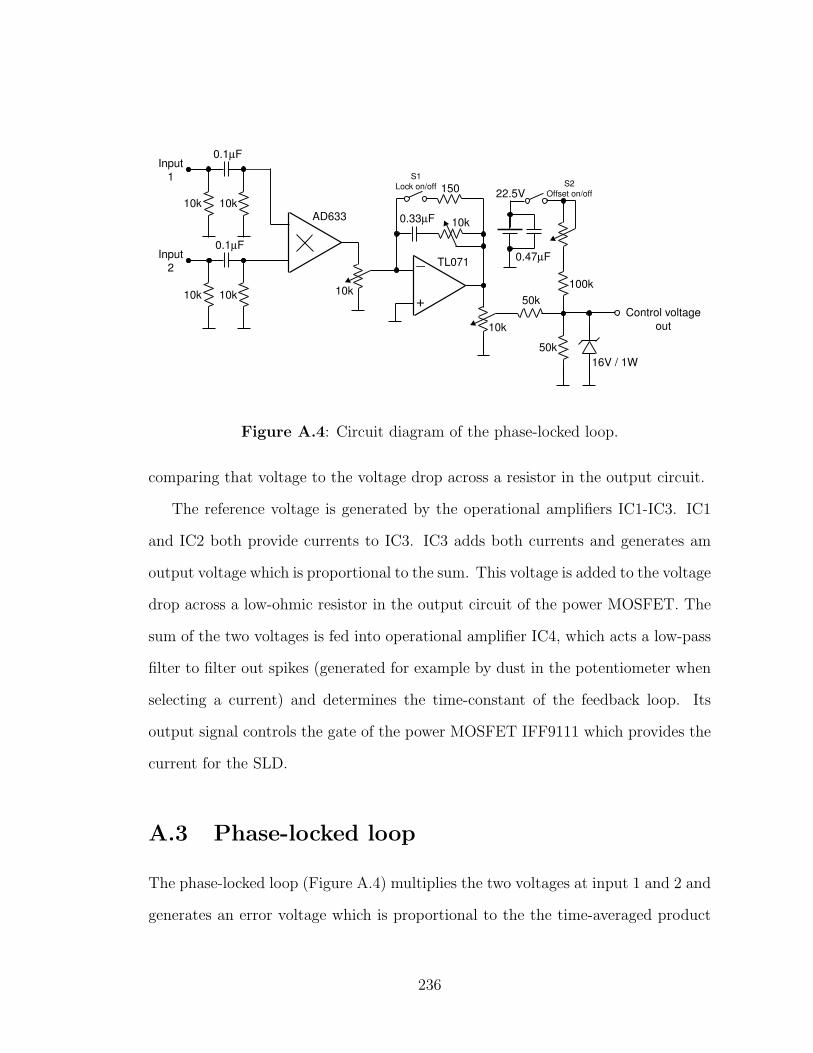
0.1µF

0.1µF

10k

10k

10k

10k

150

0.33µF 10k

10k

10k

50k

50k

100k

0.47µF

22.5V

S1 Lock on/off S2

Offset on/off

16V / 1W

AD633

TL071

Control voltage out

Input 1

Input 2

Figure A.4: Circuit diagram of the phase-locked loop.

comparing that voltage to the voltage drop across a resistor in the output circuit.

The reference voltage is generated by the operational amplifiers IC1-IC3. IC1

and IC2 both provide currents to IC3. IC3 adds both currents and generates am

output voltage which is proportional to the sum. This voltage is added to the voltage

drop across a low-ohmic resistor in the output circuit of the power MOSFET. The

sum of the two voltages is fed into operational amplifier IC4, which acts a low-pass

filter to filter out spikes (generated for example by dust in the potentiometer when

selecting a current) and determines the time-constant of the feedback loop. Its

output signal controls the gate of the power MOSFET IFF9111 which provides the

current for the SLD.

A.3 Phase-locked loop

The phase-locked loop (Figure A.4) multiplies the two voltages at input 1 and 2 and

generates an error voltage which is proportional to the the time-averaged product

236

of both voltages. This voltage is added to an offset-voltage provided by a battery;

that sum is available at the ’Control voltage out’ connector.

The high-passes at the inputs of multiplier AD633 block DC contributions and

low-frequency noise. The fraction of the output voltage of the multiplier selected

by the potentiometer is fed into a low-pass. The amplitude of the output voltage is

selected by the Amplitude potentiometer. An offset voltage, which sets the center

frequency of the AO-drivers, is added and the sum of both voltages is sent to the

output connector of the PLL.

237

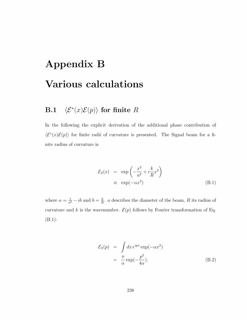
Appendix B

Various calculations

B.1 〈E∗(x)E(p)〉 for finite R

In the following the explicit derivation of the additional phase contribution of

〈E∗(x)E(p)〉 for finite radii of curvature is presented. The Signal beam for a fi-

nite radius of curvature is

ES(x) = exp

(−x2

a2+ i

k

Rx2

)

≡ exp(−αx2) (B.1)

where α = 1a2 − ib and b = k

R. a describes the diameter of the beam, R its radius of

curvature and k is the wavenumber. E(p) follows by Fourier transformation of Eq.

(B.1):

ES(p) =

∫dx eipx exp(−αx2)

=π

αexp(− p2

4α). (B.2)

238

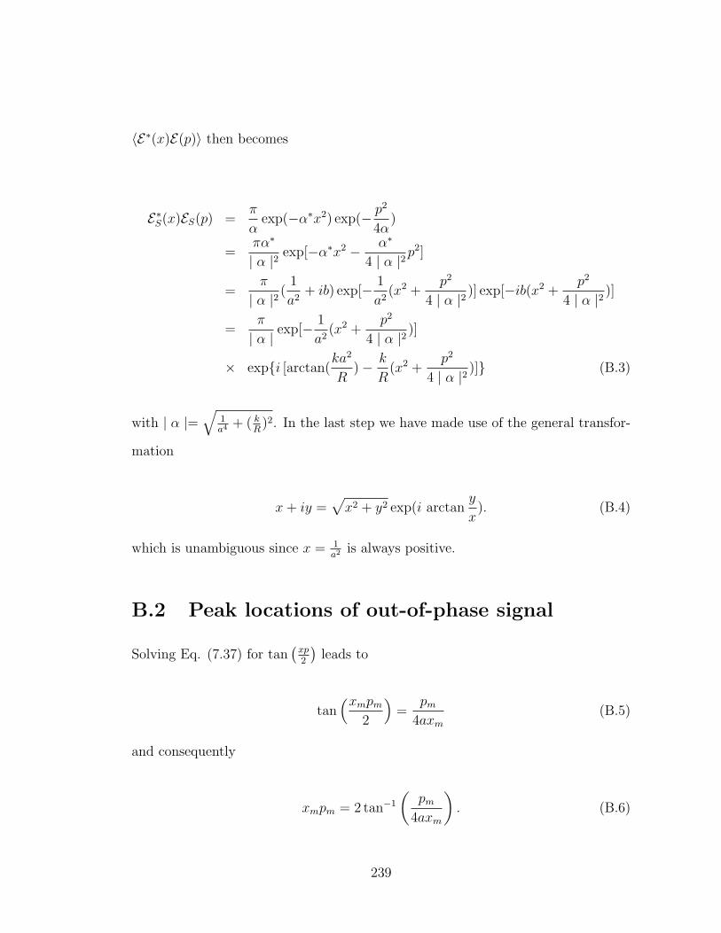
〈E∗(x)E(p)〉 then becomes

E∗S(x)ES(p) =π

αexp(−α∗x2) exp(− p2

4α)

=πα∗

| α |2 exp[−α∗x2 − α∗

4 | α |2p2]

=π

| α |2 (1

a2+ ib) exp[− 1

a2(x2 +

p2

4 | α |2 )] exp[−ib(x2 +p2

4 | α |2 )]

=π

| α | exp[− 1

a2(x2 +

p2

4 | α |2 )]

× expi [arctan(ka2

R)− k

R(x2 +

p2

4 | α |2 )] (B.3)

with | α |=√

1a4 + ( k

R)2. In the last step we have made use of the general transfor-

mation

x + iy =√

x2 + y2 exp(i arctany

x). (B.4)

which is unambiguous since x = 1a2 is always positive.

B.2 Peak locations of out-of-phase signal

Solving Eq. (7.37) for tan(

xp2

)leads to

tan(xmpm

2

)=

pm

4axm

(B.5)

and consequently

xmpm = 2 tan−1

(pm

4axm

). (B.6)

239

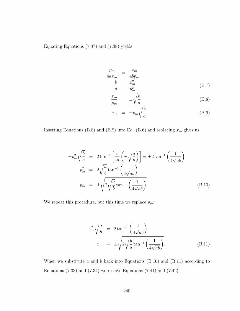
Equating Equations (7.37) and (7.38) yields

pm

4axm

=xm

4bpm

b

a=

x2m

p2m

(B.7)

xm

pm

= ±√

b

a(B.8)

xm = ±pm

√b

a. (B.9)

Inserting Equations (B.8) and (B.9) into Eq. (B.6) and replacing xm gives us

±p2m

√b

a= 2 tan−1

[1

4a

(±

√a

b

)]= ±2 tan−1

(1

4√

ab

)

p2m = 2

√a

btan−1

(1

4√

ab

)

pm = ±√

2

√a

btan−1

(1

4√

ab

). (B.10)

We repeat this procedure, but this time we replace pm:

x2m

√a

b= 2 tan−1

(1

4√

ab

)

xm = ±√

2

√b

atan−1

(1

4√

ab

). (B.11)

When we substitute a and b back into Equations (B.10) and (B.11) according to

Equations (7.33) and (7.34) we receive Equations (7.41) and (7.42):

240

xm =

√2de

x

pex

tan−1

(de

xpex

4

)(B.12)

pm =

√2pe

x

dex

tan−1

(de

xpex

4

). (B.13)

B.3 Detection of misalignment by means of SB(z)

For a perfect Gaussian-Schell source, we expect a potential phase-gradient detected

in longitudinal scans in Chapter 9 be due to different-sized beam waists of the LO’s

comprising the Dual-LO, as discussed in that chapter. In the following we assume

the phase-gradient is caused by the focused SLO.

If we set the phase of the lock-in amplifier to zero while there is a finite path-

difference ∆loff between S and the dual-LO, we can express the SB(∆l) as

SB(∆l) = exp

[−(∆l −∆loff )

2

(∆lB)2− i

∆l

z0

], (B.14)

The out-of-phase part is then

SOPB (∆l) = sin

(−∆l

z0

)exp

[−(∆l −∆loff )

2

(∆lB)2

]

=∆l

z0

exp

[−(∆l −∆loff )

2

(∆lB)2

]. (B.15)

To find the location of the peaks, we set the derivative of SOPB (∆l) to zero:

241

d

d∆lSOP

B (∆l) = 0

=1

z0

exp

[−(∆l −∆loff )

2

(∆lB)2

]

+∆l

z0

[−2

∆l − z0

(∆lB)2

]exp

[−(∆l −∆loff )

2

(∆lB)2

].

(B.16)

For this expression to vanish, the pre-factors of the exponentials must cancel:

1− 2∆l(∆l −∆loff )

(∆lB)2= 0

∆l(∆l −∆loff ) =(∆lB)2

2

∆l2 −∆l∆loff − (∆lB)2

2= 0, (B.17)

which has the two solutions

∆l1,2 =∆loff

2±

√∆l2off

4+

(∆lB)2

2. (B.18)

If we add ∆l2 and ∆l1, the square root term cancels:

∆l1 + ∆l2 = ∆loff (B.19)

If we choose the phase to be zero at the exact path-length match of S and the Dual

LO, i.e. ∆loff = 0, the peaks are symmetrically centered around this location; so

that ∆l1 + ∆l2 = 0.

The difference between ∆l2 and ∆l1 on the other hand is

242

∆l2 −∆l1 = 2

√∆l2off

4+

(∆lB)2

2

=√

∆l2off + 2(∆lB)2 (B.20)

which reproduces the result in Eq. (9.9) for ∆loff = 0.

B.4 Complex beat signal for EBS field

In the following we will derive the complex beat signal SB(dx, px) for an enhanced

backscattered field. It consists of two parts: ScohB , which describes the coherently

backscattered field (Section B.4.1), and SincohB which describes the incoherent part

of the backscattered field (Section B.4.2). The global coherence of the light of our

SLD is very high (σglob > 7), therefore we can view its light as transversely coherent.

We derive the complex beat signals for both parts separately and add them later

on.

B.4.1 Complex ScohB

In this section, we will derive the complex beat signal for the coherently backscat-

tered light of an EBS field. In the following calculations, all integrals are two-

dimensional. For simplicity, we write d2x as dx etc.

The complex beat signal is

ScohB (dx, dp) =

∫dxdp WLO(x− dx, p + k

dp

f0

) W cB(x, p) (B.21)

where

243

WLO(x−dx, p+kdp

f0

) =

∫dq

(2π)2e

iq(p+kdpf0

) 〈E∗LO(x+q

2−dx) ELO(x− q

2−dx)〉 (B.22)

and

W cohB (x, p) =

∫dp0W0(x, p0) exp[−Dt(p + p0)

2] (B.23)

with

W0(x, p0) =

∫dq′

(2π)2eiq′p0 〈E∗0 (x +

q′

2)E0(x− q′

2)〉 (B.24)

the expression for the complex beat signal follows:

ScohB (dx, dp) =

1

16π4

∫dxdqdq′

〈E∗LO(x +q

2− dx)ELO(x− q

2− dx)〉〈E∗0 (x +

q′

2)E0(x− q′

2)〉

×∫

dpdp0eiq(p+k

dpf0

)eiq′p0 exp[−Dt(p + p0)

2]. (B.25)

We measure the statistical average of 〈ELOE0〉 rather than the averages of ELO and

E0 with itself. That means we need to switch the angular brackets in the expression

above. The integral∫

dpdp0 can be simplified as follows:

244

∫dpdp0... = e

ikdpf0

q

∫dpdp0e

iqpeiq′p0 exp[−Dt(p + p0)2]

= eipxq

∫dpeiqpe−iq′p

∫dp0e

iq′p0 exp[−Dtp20]

=4π3

Dteipxq exp

(− q′2

4Dt

)δ(q − q′) (B.26)

where we replaced k dp

f0with px. Inserting the above expression and switching the

angular brackets we get:

ScohB (dx, dp) =

z20

4π2(Dt)2

∫dxdq exp(−ipxq) exp

(− q2

4Dt

)

× 〈E∗LO(x +q

2− dx)E0(x− q

2)〉〈ELO(x− q

2− dx)E∗0 (x +

q

2)〉.

(B.27)

The electric field of the Dual-LO is

ELO(x) ∝ exp

(− x2

4σ2sa

2

)+ βeiθ exp

(− x2

4σ2sA

2

):= Ea

LO(x) + βeiθEALO(x) (B.28)

and for the Signal beam

E0(x) ∝ exp

(− x2

4σ2sB

2+ i

k

2RB2x2

). (B.29)

Here we introduced scaling factors A and a for the BLO and the SLO, and B for

the Signal beam, which describe the different relative sizes of the beams. β is the

amplitude of the BLO relative to the SLO, eiθ the phase, where θ = ωt is the locking

245

frequency of the LOs.

Since the global coherence of our light source is much larger than 1 (σglob > 7),

we can set the exponential containing σg in Eq. (3.2) to 1, so that the mutual

coherence function is just the product of the electric fields itself. The product of

electrical fields in Eq. (B.27) is

〈E∗LO(x1)E0(x2)〉〈ELO(x3)E∗0 (x4)〉 = (〈Ea∗LO(x1)E0(x2)〉+ βeiθ〈EA∗

LO(x1)E0(x2)〉)

× (〈EaLO(x3)E∗0 (x4)〉+ βe−iθ〈EA

LO(x3)E∗0 (x4)〉)

(B.30)

where we replaced the variables as follows

x1 → x +q

2− dx

x2 → x− q

2

x3 → x− q

2− dx

x4 → x +q

2.

We detect the cross-terms only:

βeiθ〈EA∗LO(x1)E0(x2)〉〈Ea

LO(x3)E∗0 (x4)〉+ βe−iθ〈EALO(x3)E∗0 (x4)〉〈Ea∗

LO(x1)E0(x2)〉.(B.31)

One sees that x1 and x3 as well es x2 and x4 are identical except for the sign of q.

When we put the cross-terms back into (B.27) we get

246

ScohB (dx, dp) =

z20

4π2(Dt)2


(− q2

4Dt

)

×[βeiθEA∗

LO(x− dx +q

2)E0(x− q

2)Ea

LO(x− dx − q

2)E∗0 (x +

q

2)

+ βe−iθ〈EALO(x− dx − q

2)E∗0 (x +

q

2)〉〈Ea∗

LO(x− dx +q

2)E0(x− q

2)]

=z20

4π2(Dt)2


(− q2

4Dt

)

×[βeiθEA∗

LO(x− dx +q

2)E0(x− q

2)Ea

LO(x− dx − q

2)E∗0 (x +

q

2)]

+ c.c.

= scohB (dx, dp)+c.c (B.32)

where scohB (dx, dp) is the complex beat signal and c.c. stands for ’complex conjugate’.

If we make the following variable transformation:

η = x +q

2(B.33)

ξ = x− q

2(B.34)

we get

ScohB (dx, dp) =

z20

4π2(Dt)2

∫dη dξ exp[−i(η − ξ)px] exp

[−(η − ξ)2

4Dt

]

× EA∗LO(η − dx)E0(ξ)Ea

LO(ξ − dx)E∗0 (η). (B.35)

We now replace the electrical fields according to Equations (B.28) and (B.29):

247

EA∗LO(x1)E0(x2) ∝ exp

(− x2

1

4σ2sA

2− x2

2

4σ2sB

2− ik

2R

x22

B2

)(B.36)

≡ exp(−vAx21 − vBx2

2) (B.37)

where we replaced the terms in the first line according with vA and vB in the second

line. The second product of electrical fields in Eq. (B.35) is replaced accordingly,

so that

1

4σ2sA

2→ vA (B.38)

1

4σ2sa

2→ va (B.39)

1

4σ2sB

2− ik

2RB→ vB (B.40)

(B.41)

and

ScohB (dx, dp) =

z20

4π2(Dt)2

∫dη dξ exp[−i(η − ξ)px] exp

[−(η − ξ)2

4Dt

]

× exp[−(η − dx)2vA − ξ2vB] exp[−(ξ − dx)

2va − η2v∗B] (B.42)

= scohB (dx, dp) + c.c. (B.43)

After straight-forwardly solving the two Gaussian integrals we get for the complex

beat signal

248

scohB (dx, dp) =

z20

4(Dt)2

α

vA + vB + β

× exp−d2

x(vA + va) + α(vAdx − ipx

2)2

+

[(va + vAα

4Dt)dx + i2Dtβpx

]2

va + vB + β

(B.44)

where

α =1

14Dt

+ vA + v∗B(B.45)

β =1

4Dt + 1vA+v∗B

. (B.46)

Again, the in-phase quadrature signal is the real part of scohB (dx, dp) in Eq. (B.44),

the out-of-phase signal is its imaginary part. Out of conformity, we will use ScohB (dx, dp)

instead of scohB (dx, dp) to denote the complex beat signal.

B.4.2 Complex SincohB

In this section we are going to derive the incoherently backscattered light of an EBS

field, commonly referred to as the ’incoherent background’. Again, all integrals in

the following are two-dimensional; we write dx instead of d2x for simplicity.

The complex beat signal can be written as

SincohB (dx, dp) ∝

∫dxdp WLO(x− dx, p + k

dp

f0

) W incohB (x, p) (B.47)

where

249

WLO(x−dx, p+kdp

f0

) =

∫dq

(2π)2e

iq(p+kdpf0

) 〈E∗LO(x+q

2−dx) ELO(x− q

2−dx)〉 (B.48)

and

W incohB (x) =

z20

(4π)3/2(Dt)3/2

∫dx′

∫dp′W0(x

′, p′)exp

[−(x− x′)2

4Dt

](B.49)

with

W0(x′, p′) =

∫dq′

(2π)2eiq′p′ 〈E∗0 (x′ +

q′

2)E0(x

′ − q′

2)〉. (B.50)

Inserting Equations (B.47)-(B.49) into Eq. (B.50) yields

SincohB (dx, dp) =

1

(2π)4

z20

(4π)3/2(Dt)5/2

∫dxdpdx′dp′dqdq′

× eiq(p+px) exp

[−(x− x′)2

4Dt

]eiq′p′

× 〈E∗LO(x +q

2− dx)ELO(x− q

2− dx)E∗0 (x′ +

q′

2)E0(x

′ − q′

2)〉.

(B.51)

∫dpeiqp

∫dp′eiq′p′ are replaced by delta functions, yielding

250

SincohB (dx) =

z20

(4π)3/2(Dt)5/2

∫dxdx′

exp

[−(x− x′)2

4Dt

]〈E∗LO(x− dx)E0(x

′)〉〈ELO(x− dx)E∗0 (x′)〉

(B.52)

where 〈...〉〈...〉 =| 〈...〉 |2. We again express the mutual coherence functions as the

product of the Signal- and LO-fields in Equations (B.28) and (B.29). The product

of the electrical fields is of the form as in Eq. (B.30), and again we detect only the

cross-terms shown in Eq. (B.31). Replacing the electrical fields in this equations

according to Eq. (B.37), we get

SincohB (dx) =

z20

(4π)3/2(Dt)5/2

∫dxdx′

exp

[−(x− x′)2

4Dt

]

× exp[−vA(x− dx)2 − vB(x′)2 − va(x− dx)

2 − v∗B(x′)2] (B.53)

Solving the two Gaussian integrals is again very straight-forward; after a few lines

of transformation one gets:

SincohB (dx) =

√π

4

z20

(Dt)3/2

1

(vB + v∗B)(vA + va)

× exp

(− d2

x1

vA+va+ 1

vB+v∗B+ 4Dt

). (B.54)

251

Appendix C

C++ codes

C.1 Inverse Margenau-Hill transformation

I wrote the following program code to retrieve the Wigner function from the mea-

sured complex beat signal.

const ppoints=901;

// insert number of points in p

const xpoints=901;

// insert number of points in x

double x,p, x0,p0, dxmax,dpmax, dxcrop, dpcrop, kcorr, dummy;

double i,j, n,m, nmin,nmax, mmin,mmax, nspan,mspan;

double IPnum[ppoints+1][xpoints+1], OOPnum[ppoints+1][xpoints+1];

FILE *ifp, *jfp, *outfp;

int main(void)

252

// insert dxmax, pxmax

dxmax = 500*9*0.00005;

dpmax = 75*9*0.00005/60*1000; kcorr=9263.1*0.001;

cout << "Fourier transformation of IP and OOP

into Wigner function\nFrank Reil\n\n";

if (( ifp=fopen("iplist1.dat","r")) == NULL)

printf("Can’t open iplist.dat\\n");

exit(1);

if (( jfp=fopen("ooplist1.dat","r")) == NULL)

printf("Can’t open ooplist.dat\n");

exit(1);

for(n=1; n<=xpoints; n++)

for(m=1; m<=ppoints; m++)

fscanf(ifp, "%lf", &IPnum[int(m)][int(n)]);

fscanf(jfp, "%lf", &OOPnum[int(m)][int(n)]);

253

nmin = 1;

nmax = xpoints; mmin = 1;

mmax = ppoints; nspan = nmax - nmin;

mspan = mmax - mmin;

if (( outfp=fopen("outlist.dat","w")) == NULL)

printf("Can’t open iplist.dat\n");

exit(1);

for(x=-dxmax; x<=dxmax*1.001; x+=0.04*dxmax)

for(p=-dpmax; p<=dpmax*1.001; p+=0.04*dpmax)

dummy=0;

for(n=1; n<=xpoints; n++)

for(m=1; m<=ppoints; m++)

dummy += IPnum[int(m)][int(n)]

*cos(2*kcorr*(x-(2*(n-nmin)/nspan-1)*dxmax)

*(p-(2*(m-mmin)/mspan-1)*dpmax))

+OOPnum[int(m)][int(n)]

*sin(2*kcorr*(x-(2*(n-nmin)/nspan-1)*dxmax)

*(p-(2*(m-mmin)/mspan-1)*dpmax));

254

fprintf(outfp, "%lf\n",dummy);

printf("%lf\n",dummy);

fclose(outfp);

C.2 Time-resolved single-scattering in transmis-

sion

For very dilute solutions, where the mean free path is comparable to or larger than

the sample length, the single-scatter model can be applied. Figure C.1 shows a ray

entering a sample container of length d from the left, getting scattered once and

leaving the container. The path-length in the medium is determined by the chosen

path-delay ∆L of corner-cube C1 in the experiment (see Figure 5.6).

The phase-space coordinates are

x = r1 sin θ (C.1)

p = sin θ (C.2)

The difference between r1 and z1 is just the selected path-delay ∆l:

255

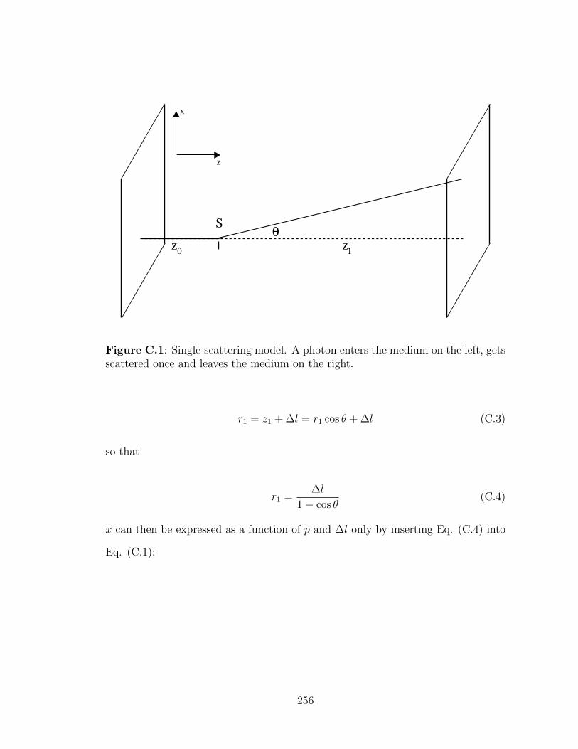
z

x

θS

z 1 z 0

r1

z=dz=0

x

Figure C.1: Single-scattering model. A photon enters the medium on the left, getsscattered once and leaves the medium on the right.

r1 = z1 + ∆l = r1 cos θ + ∆l (C.3)

so that

r1 =∆l

1− cos θ(C.4)

x can then be expressed as a function of p and ∆l only by inserting Eq. (C.4) into

Eq. (C.1):

256

x = r1 sin θ

= ∆lsin θ

1− cos θ

= ∆l1 + cos θ

sin θ

= ∆l1 +

√1− (p/k)2

p/k

= ∆l

(1

p/k+

√1

(p/k)2− 1

)(C.5)

≈ ∆l2

p/k, (p/k)2 ¿ 1 (C.6)

which is a hyperbola. The approximation in Eq. (C.6) has an accuracy of better

than 1% for the momentum range we measure. Figure 13.4(c) shows a plot of Eq.

(C.5) for a path-delay of ∆l = 100 µm in air. The valid range for Eq. (C.5) is

restricted by the cell size d:

r1 cos θ < d (C.7)

which is equivalent to

1√1− (p/k)2

− 1 >∆l

d. (C.8)

C.2.1 Calculation of xmax

The transverse position x can be expressed as a function of z1:

x2 = r21 − z2

1 = (z1 + ∆l)2 − z21 . (C.9)

257

Simplifying yields

x =√

2z1∆l + (∆l)2 (C.10)

Eq. (C.10) shows that the earlier the photon scatters, the larger the transverse

position of the scattered photon at the sample output plane. The maximal trans-

verse position xmax results when the photon scatters right after entering the turbid

medium, i.e. for z1 = L = 10mm:

xmax =√

2L∆l + (∆l)2. (C.11)

C.3 Time-resolved double-scattering in transmis-

sion

The time-dependent Double-Scattering algorithm I developed is a Monte-Carlo com-

puter algorithm that calculates the intensity at the sample output as a function of

position and momentum for an incident light ray, as a function of path delay. The

output intensity of a finite-sized collimated beam can then be calculated by con-

volving the input beam numerically with the calculated ’Green-function’.

Figure C.2 shows two scatterers in a sample container of length d. The ray

comes in from the left, scatters at the first scatterer S1 at z0 and then at the second

scatterer S2 at z0 + z1. From there it travels to the output surface and leaves the

medium.

The intensity distribution at z = d is rotationally invariant with respect to φ1,

we therefore choose φ1 = π/2, which fixed the scattering at S1 in the y − z-plane,

and rotate the intensity distribution after the rest of the calculation is done.

258

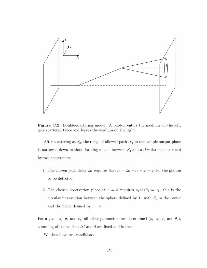
z

y

x

θ

φθ2

1

2

r2

S1

S2

z

r1

z z1 20

r1 sin(θ )1

z=dz=0

Figure C.2: Double-scattering model. A photon enters the medium on the left,gets scattered twice and leaves the medium on the right.

After scattering at S2, the range of allowed paths r2 to the sample output plane

is narrowed down to those forming a cone between S2 and a circular cone at z = d

by two constraints:

1. The chosen path delay ∆l requires that r2 = ∆l− r1 + z1 + z2 for the photon

to be detected

2. The chosen observation place at z = d requires r2 cos θ2 = z2, this is the

circular intersection between the sphere defined by 1. with S2 in the center

and the plane defined by z = d.

For a given z0, θ1 and r1, all other parameters are determined (z1, z2, r2 and θ2),

assuming of course that ∆l and d are fixed and known.

We thus have two conditions:

259

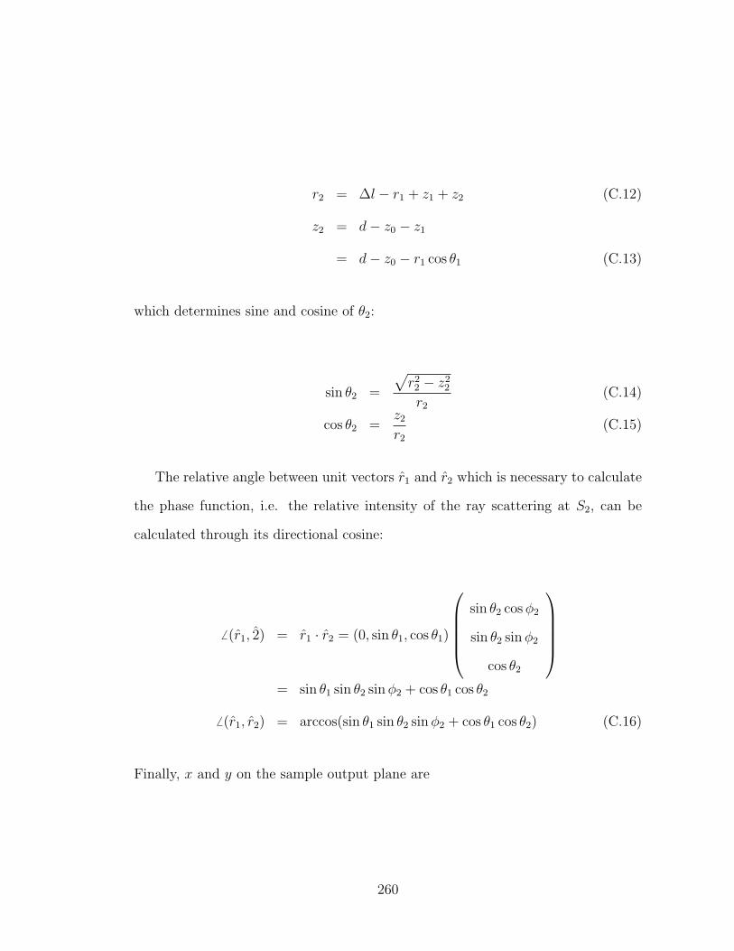
r2 = ∆l − r1 + z1 + z2 (C.12)

z2 = d− z0 − z1

= d− z0 − r1 cos θ1 (C.13)

which determines sine and cosine of θ2:

sin θ2 =

√r22 − z2

2

r2

(C.14)

cos θ2 =z2

r2

(C.15)

The relative angle between unit vectors r1 and r2 which is necessary to calculate

the phase function, i.e. the relative intensity of the ray scattering at S2, can be

calculated through its directional cosine:

6 (r1, 2) = r1 · r2 = (0, sin θ1, cos θ1)

sin θ2 cos φ2

sin θ2 sin φ2

cos θ2

= sin θ1 sin θ2 sin φ2 + cos θ1 cos θ2

6 (r1, r2) = arccos(sin θ1 sin θ2 sin φ2 + cos θ1 cos θ2) (C.16)

Finally, x and y on the sample output plane are

260

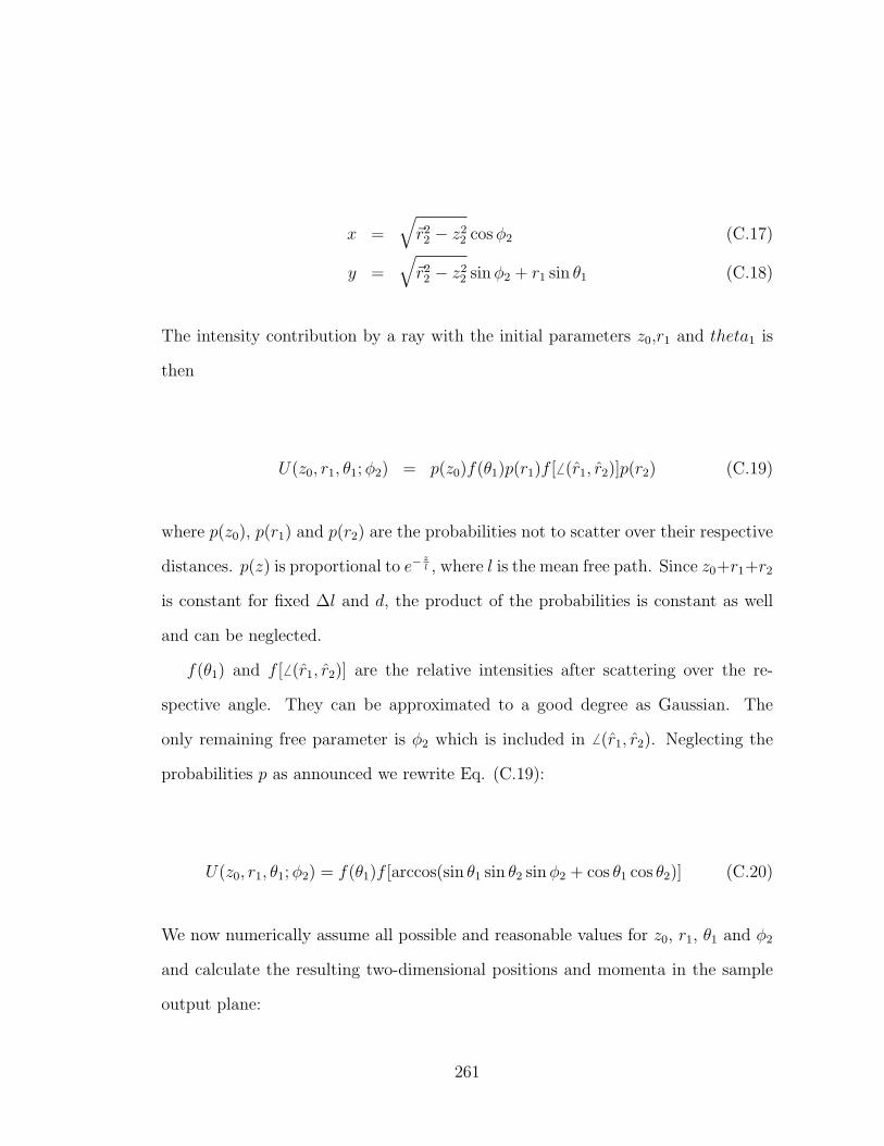
x =√

~r22 − z2

2 cos φ2 (C.17)

y =√

~r22 − z2

2 sin φ2 + r1 sin θ1 (C.18)

The intensity contribution by a ray with the initial parameters z0,r1 and theta1 is

then

U(z0, r1, θ1; φ2) = p(z0)f(θ1)p(r1)f [6 (r1, r2)]p(r2) (C.19)

where p(z0), p(r1) and p(r2) are the probabilities not to scatter over their respective

distances. p(z) is proportional to e−zl , where l is the mean free path. Since z0+r1+r2

is constant for fixed ∆l and d, the product of the probabilities is constant as well

and can be neglected.

f(θ1) and f [6 (r1, r2)] are the relative intensities after scattering over the re-

spective angle. They can be approximated to a good degree as Gaussian. The

only remaining free parameter is φ2 which is included in 6 (r1, r2). Neglecting the

probabilities p as announced we rewrite Eq. (C.19):

U(z0, r1, θ1; φ2) = f(θ1)f [arccos(sin θ1 sin θ2 sin φ2 + cos θ1 cos θ2)] (C.20)

We now numerically assume all possible and reasonable values for z0, r1, θ1 and φ2

and calculate the resulting two-dimensional positions and momenta in the sample

output plane:

261

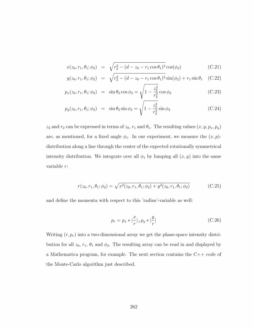
x(z0, r1, θ1; φ2) =√

r22 − (d− z0 − r1 cos θ1)2 cos(φ2) (C.21)

y(z0, r1, θ1; φ2) =√

r22 − (d− z0 − r1 cos θ1)2 sin(φ2) + r1 sin θ1 (C.22)

px(z0, r1, θ1; φ2) = sin θ2 cos φ2 =

√1− z2

2

r22

cos φ2 (C.23)

py(z0, r1, θ1; φ2) = sin θ2 sin φ2 =

√1− z2

2

r22

sin φ2 (C.24)

z2 and r2 can be expressed in terms of z0, r1 and θ1. The resulting values (x, y, px, py)

are, as mentioned, for a fixed angle φ1. In our experiment, we measure the (x, p)-

distribution along a line through the center of the expected rotationally symmetrical

intensity distribution. We integrate over all φ1 by lumping all (x, y) into the same

variable r:

r(z0, r1, θ1; φ2) =√

x2(z0, r1, θ1; φ2) + y2(z0, r1, θ1; φ2) (C.25)

and define the momenta with respect to this ’radius’-variable as well:

pr = px ∗ |xr|+py ∗ |y

r| (C.26)

Writing (r, pr) into a two-dimensional array we get the phase-space intensity distri-

bution for all z0, r1, θ1 and φ2. The resulting array can be read in and displayed by

a Mathematica program, for example. The next section contains the C++ code of

the Monte-Carlo algorithm just described.

262

C.3.1 C++ Code

#include <iostream> #include <math.h> #include <stdio.h>

using namespace std;

// good values are:

// thetamax: 7*theta0

// zstep: zmax/40

// r1step: r1max/40

// phi2step: 0.005;

// theta1step: theta0/80

const double Pi=3.1415926;

const double mu = 3.33; // transport mean free path [mm]

const double lstar = 1.96; // mean free path [mm]

const double theta0 = 0.412;

// angular width [rad] of scatter, was 0.0396 until Oct 5,02

const double thetamax = 10*theta0;

// [rad] upper bound for theta we use const

double thetamaxsq = pow(thetamax,2);

const double d=10;

// length of sample [mm]

const double dell=0.1/1.33; // path delay [mm]

const double zmin = 0.01*lstar; // [mm]

const double zmax = d; // [mm]

263

const double zstep=zmax/57;

// constant makes for loop faster

const double r1min = 0.1*lstar;

const double r1max = 2.43*d; // was d

const double r1step=r1max/49

const double phi2step=0.007; // was 0.005

const double theta1step=theta0/110;

double z0,z1,z2, r1,r2, theta1, theta2, phi2, rho1, rho2;

double x, y, r, px, py, pr;

double sintheta1,costheta1, sintheta2, costheta2, sinphi2, cosphi2;

double integphi1, integphi, spatpartial, rperp;

double shift, beamradi, bsteps, expfac;

double U[600][600]; // [r,px]

int rintel, pintel; int cr;

FILE *Ufp, *Vfp;

int main(void) cout << "Monte-Carlo Simulation of two-scatter events

in turbid medium, time resolved\nFrank Reil\n\n";

if (( Ufp=fopen("outarray.dat","w")) == NULL)

printf("Can’t open outarray.dat\n");

exit(1);

264

if (( Vfp=fopen("genauarray.dat","w")) == NULL)

printf("Can’t open genauarray.dat\n"); exit(1);

for(z0=zmin; z0<zmax; z0+=zstep)

printf("z0 = %lf*d\n ...",z0/d);

for(theta1=-thetamax; theta1<thetamax; theta1+=theta1step)

sintheta1 = sin(theta1);

costheta1 = cos(theta1);

for(r1=0; r1<r1max; r1+=r1step)

z1=r1*costheta1;

z2 = d - z0 - z1;

if (z2>0)

r2 = z1 + z2 + dell - r1;

if (z2<=r2) // r2<0 statement superfluous

spatpartial = exp(-z0/mu)*(1-exp(-z0/mu)) * exp(-r1/mu)

*(1-exp(-r1/mu)) * exp(-r1/mu)*(1-exp(-r1/mu));

// replaced r2 by r1

sintheta2 = sqrt(1 - pow(z2,2)/pow(r2,2));

costheta2 = z2/r2;

rperp = sqrt(pow(r2,2) - pow(z2,2));

265

for(phi2=-Pi; phi2<=Pi; phi2+=phi2step)

// that will give all radii with x positive !

cosphi2 = cos(phi2);

sinphi2 = sin(phi2);

if (rperp*sinphi2 + r1*sin(theta1) > 0)

integphi=exp(-pow(acos(sintheta1*sinphi2*sintheta2

+ costheta1*costheta2),2)/thetamaxsq);

integphi1=exp(-pow(theta1,2)/thetamaxsq);

x = rperp*sinphi2 + r1*sin(theta1);

y = rperp*cosphi2;

r = sqrt(pow(y,2) + pow(x,2));

px = sintheta2*cosphi2;

py = sintheta2*sinphi2;

pr = px*abs(x/r) + py*abs(y/r);

// projection of (px,py) on r, where we measure everything.

// should be independent of sign of x and y

if (pr<15000000 && pr>0)

U[int(r*74)][300+int(pr*50000)]

+=1000000*integphi*integphi1*spatpartial;

// if (rperp*sinphi2 + r1*sin(theta1) > 0)

// phi2-loop

// if (z2<=r2)

// if (z2>0)

266

// r1-forloop

beamradi=0.1/1 * 74; // intensity: radius in mm times 100 pts/mm

bsteps = beamradi/20;

for (shift=-2*beamradi; shift<=2*beamradi; shift+=bsteps)

expfac = exp(-pow(shift/beamradi,2)); // Gaussian factor

for (rintel=0; rintel<=200; rintel++)

if (rintel+shift > 0)

for (pintel=200; pintel<=400; pintel++)

U[rintel][pintel]+=U[rintel+int(shift)][pintel]*expfac;

for(rintel=0; rintel<=200; rintel++)

for(pintel=200; pintel<=400; pintel++) // 300 is px=0

fprintf(Ufp, "%lf\n", U[rintel][pintel]);

fclose(Ufp);

267

Appendix D

Speckle

Figure D.1 shows the quadrature signals for a scan of a speckle field which was

generated by shining a Gaussian SLD beam on to a glass containing tiny air bubbles.

The smallest range (bottom row) presents a view inside a speckle; the product of

position- and momentum range is

0.5 mm× 1.3 mrad = 650 nm (D.1)

which is smaller than the wavelength of 678.3 nm we use. The same phase-space

are scanned by only the BLO and only the SLO is shown in Figure D.2. Clearly,

the resolution provided by a single LO is not sufficient to resolve the speckle. The

Wigner function retrieved from the quadrature signals in Figure D.1 is shown in

Figure D.3.

268

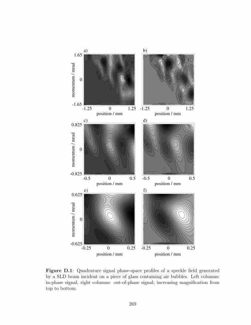
-1.25 0 1.25

1.65

0

-1.65-1.25 0 1.25

0.825

0

-0.825-0.5 0 0.5 -0.5 0 0.5

0.625

0

-0.625-0.25 0 0.25 -0.25 0 0.25




mom

entu

m /

mra

dm

omen

tum

/ m

rad

mom

entu

m /

mra

d

a) b)

c) d)

e) f)

Figure D.1: Quadrature signal phase-space profiles of a speckle field generatedby a SLD beam incident on a piece of glass containing air bubbles. Left columns:in-phase signal, right columns: out-of-phase signal; increasing magnification fromtop to bottom.

269

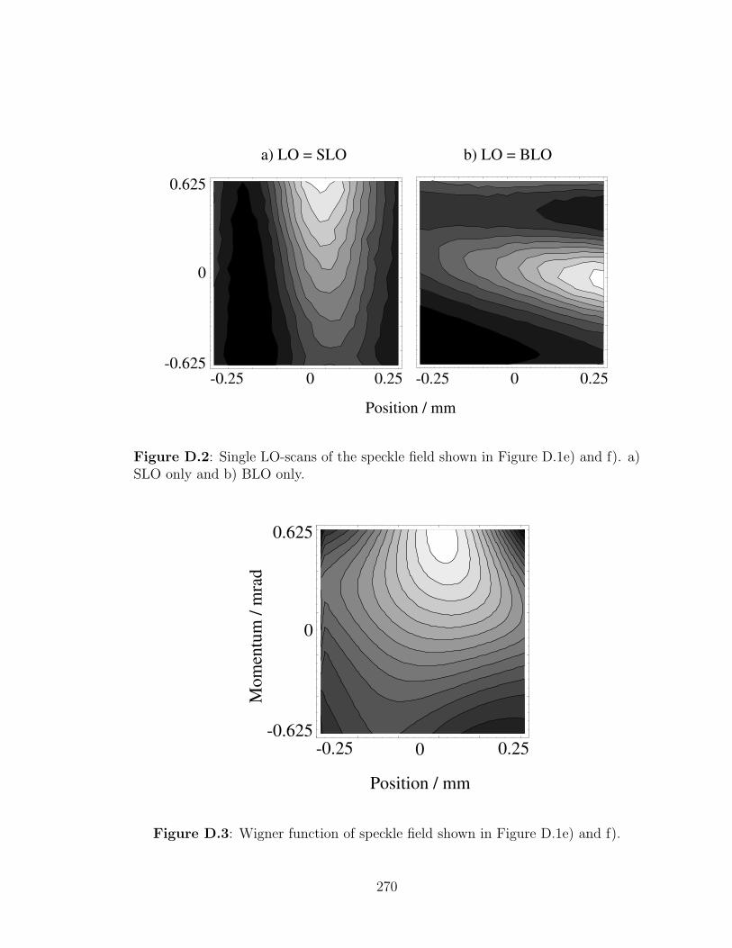
-0.25 0.250 -0.25 0.250

0.625

-0.625

0

Position / mm

a) LO = SLO b) LO = BLO

Figure D.2: Single LO-scans of the speckle field shown in Figure D.1e) and f). a)SLO only and b) BLO only.

-0.25 0.250

0.625

-0.625

0

Mom

entu

m /

mra

d

Position / mm

Figure D.3: Wigner function of speckle field shown in Figure D.1e) and f).

270

Bibliography

[1] K. F. Lee, F. Reil, S. Bali, A. Wax, and J. E. Thomas. Heterodyne measurementof wigner distributions for classical optical fields. Opt. Lett., 24:1370, 1999.

[2] A. Wax, S. Bali, G. A. Alphonse, and J. E. Thomas. Characterizing the coher-ence of broadband sources using optical phase space contours. J. Biomed.Opt., 4:482, 1999.

[3] A. Wax, S. Bali, and J. E. Thomas. Optical phase-space distributions forlow-coherence light. Opt. Lett., 24:1188, 1999.

[4] A. Wax, S. Bali, and J. E. Thomas. Time-resolved phase-space distributionsfor light backscattered from a disordered medium. Phys. Rev. Lett., 85:66,2000.

[5] A. Wax. Optical phase space distributions for coherence tomography. Ph.D.Dissertation, Duke University, 1999, unpublished.

[6] S. K. Gayen, M. E. Zevallos, B. B. Das, and R. R. Alfano. Time-sliced transil-lumination imaging of normal and cancerous breast tissues. OSA Trendsin Optics and Photonics on Advanaces in Optical Imaging and PhotonMigration, 21:63–66, 1998.

[7] H. Rinneberg, D. Grosenick, H. Wabnitz, H. Danlewski, K. Moesta, andP. Schlag. Time-domain optical mammography: results on phantoms,healthy volunteers and patients. OSA Trends in Optics and Photonics onAdvanaces in Optical Imaging and Photon Migration, 21:278–280, 1998.

[8] J. C. Hebden and S. R. Arridge. Imaging through scattering media by the useof an analytical model of perturbation amplitudes in the time domain.Appl. Opt., 35:6788–6796, 1996.

[9] Jeremy C. Hebden. http://www.medphys.ucl.ac.uk/research/borg/research/fundedprojects/jemfell.htm. Website.

[10] K. M. Yoo and R. R. Alfano. Time-resolved coherent and incoherent compo-nents of forward light scattering in random media. Opt. Lett., 15:320–322,1990.

271

[11] M. S. Patterson, B. Chance, and B. C. Wilson. Time resolved reflectance andtransmittance for the non-invasive measurement of tissue optical proper-ties. Appl. Opt., 28:2331–2336, 1989.

[12] K. M. Yoo, B. B. Das, and R. R. Alfano. Imaging of a translucent object hid-den in a highly scattering medium from the early portion of the diffusivecomponent of a transmitted ultrafast laser pulse. Opt. Lett., 17:958–960,1992.

[13] Hamamatsu Co. Streak cameras and their features,http://usa.hamamatsu.com/sys-streak/operating/default.htm. Web-site.

[14] L. Wang, P. P. Ho, X. Liang, H. Dai, and R. R. Alfano. Kerr-fourier imagingof hidden objects in thick turbid media. Opt. Lett, 18:241–243, 1993.

[15] L. Wang, P. P. Ho, C. Liu, G. Zhang, and R. R. Alfano. Ballistic 2-d imagingthrough scattering walls using and ultrafast opical kerr gate. Science,253:769–771, 1991.

[16] Y. Wang J. Wu, L. Perelman, I. Itzkan, R. R. Dasari, and Michael Feld. Time-resolved multichannel imaging of fluorescent objects embedded in turbidmedia. Opt. Lett., 20:489–491, 1995.

[17] A. Yodh and B. Chance. Spectroscopy and imaging with diffusing light. PhysicsToday, 48(3):34–40, 1995.

[18] M. A. O’Leary, D. A. Boas, B. Chance, and A. G. Yodh. Refraction of diffusephoton density waves. Phys.Rev.Lett., 69:2658–2661.

[19] D. A. Boas, M. A. O’Leary, B. Chance, and A. G. Yodh. Scattering andwavelength transduction of diffuse photon density waves. Phys. Rev. E,47:2999–3002, 1993.

[20] J. M. Schmitt, A. Knuttel, and J. R. Knutson. Interference of diffusive lightwaves. J. Opt.Soc.Am.A, 9:1832–1843, 1992.

[21] B. W. Pogue, M. Testorf, U. L. Osterberg, and K. Paulsen. Development ofquantitative imaging in frequency-domain diffuse optical tomography forbreast cancer detection. OSA Trends in Optics and Photonics on Advancesin Optical Imaging and Photon Migration, 21:245–250, 1998.

[22] X. D. Li, J. P. Culver, T. Durduran, B. Chance, A. G. Yodh, and D. N.Pattanayak. Diffraction tomography with diffuse photon density waves:Clinical studies and background subtraction. OSA Trends in Optics and

272

Photonics on Advances in Optical Imaging and Photon Migration, 21:281–283, 1998.

[23] S. Fantini, S. A. Walker, M. A. Franceschini, A. E. Cerussi, J. Edler, K. T.Moesta, P. M. Schlag, M. Kaschke, and E. Gratton. Optical characteriza-tion of breast tumors by frequency-domain optical mammography. OSATrends in Optics and Photonics on Advances in Optical Imaging and Pho-ton Migration, 21:289–293, 1998.

[24] Kottan Labs. http://kottan-labs.bgsu.edu/presentations/modspec1-wg.htm.Website.

[25] Florida State University. http://www.microscopy.fsu.edu/primer/techniques/fluorescence/multiphoton/multiphotonhome.html. Website.

[26] Kentech Company. http://www.kentech.co.uk/fluorlifeimage.html. Website.

[27] W. M. Keck Center for Cellular Imaging/University of Virginia.http://www.cci.virginia.edu/flimtheory.html. Website.

[28] The Photonics Center. http://www.thephotonicscenter.com/new/laboratories.Website.

[29] W. M. Keck Center for Cellular Imaging/University of Virginia.http://www.cci.virginia.edu/decon.html. Website.

[30] Worcester Polytechnic Institute N. Kildahl.http://www.wpi.edu/academics/depts/chemistry/courses/ch2670/infrared.html. Website.

[31] Michigan State University William Reusch.http://www.cem.msu.edu/ reusch/OrgPage/VirtualText/Spectrpy/InfraRed/infrared.htm. Website.

[32] Inphotonics.com. http://www.inphotonics.com/raman.htm. Website.

[33] Austria FELMI-ZFE, Technische Universitaet Graz.http://www.cis.tugraz.at/felmi/researchraman.html. Website.

[34] Physics Department at University of Parma Danilo Bersani.http://www.fis.unipr.it/ bersani/raman/raman/ramtutor.htm. Website.

[35] Robert H. Webb. Confocal optical microscopy. Rep. Prog. Phys., pages 427–471, 1996.

[36] W. M. Keck Center for Cellular Imaging/University of Virginia.http://www.cci.virginia.edu/confocaltheory.html. Website.

273

[37] Digital Instruments. Applications to atomic force microscopy,http://www.veeco.com/pdf/clmain.pdf. Website, 1998/99.

[38] Joseph A. Izatt, Manish D. Kulkarni, Kenji Kobayashi, Michael V. Sivak, Jen-nifer K. Barton, and Ashley J. Welch. Optical coherence tomography forbiodiagnostics. Optics & Photonics News, pages 41–47, May 1997.

[39] J. A. Izatt and M. D. Kulkarni. Doppler flow imaging using optical coherencetomography. presented at OSA Conference on Lasers and Electro-Optics,Anaheim, CA, 1006, post-deadline paper CPD3-1.

[40] Z. Chen et. al. Optical doppler tomographic imaging of fluid flow velocity inhighly scattering media. Opt. Lett., 22:64–66, 1997.

[41] Martin J. Bastiaans. Application of the wigner distribution function to partiallycoherent light. J. Opt. Soc. A, 3:1227, 1986.

[42] Chung-Chieh Cheng and M. G. Raymer. Long-range saturation of spatial de-coherence in wave-field transport in random multiple-scattering media.Phys. Rev. Lett., 82:4807, 1999.

[43] Leonard Mandel and Emil Wolf. Optical Coherence and Quantum Optics. Cam-bridge University Press, 1995.

[44] Charles Kittel and Herbert Kroemer. Thermal physics. W.F. Freeman andCompany, 1980.

[45] Martin J. Bastiaans. Second-order moments of the wigner distribution functionin first-order optical systems. Optik, 88:163–168, 1991.

[46] A. Wax and J. E. Thomas. Optical heterodyne imaging and wigner phase spacedistributions. Opt. Lett, 21:1427–1429, 1996.

[47] Melles Griot. Tutorial. Catalog.

[48] photonics.com. Tutorial, http://www.photonics.com. Website.

[49] email exchange with Vladimir Shidlovski from Superlum Co.

[50] Peter W. Milonni and Joseph H. Eberly. Lasers. John Wiley and Sons, 1988.

[51] V. K. Batovrin, I. A. Garmash, V. M. Gelikonov, G. V. Gelikonov, A. V.Lyubarskii, A. G. Plyavenek, S. A. Safin, A. T. Semonov, V. R.Shidlovskii, M. V. Shramenko, and S. D. Yakubovich. Superluminescentdiodes based on single-quantum-well (gaal)as heterostructures. Quantumelectronics, 26(2):109–114, 1996.

274

[52] Akira Ishimaru. Wave propagation and scattering in random media. Academicpress, 1978.

[53] M. Kerker. The Scattering of Light and Other Electromagnetic Radiation. Aca-demic Press, 1969.

[54] Craig F. Bohren and Donald R. Huffman. Absorption and scattering of lightby small particles. Wiley-Interscience, 1983.

[55] Diederik S. Wiersma, Paolo Bartolini, Ad Lagendijk, and Roberto Righini.Localization of light in a disordered medium. Nature, 390:671–673, 1997.

[56] P. W. Anderson. The question of classical localization: a theory of white paint?Phil. Mag. B, 52:505–509, 1095.

[57] E. Abrahams, P. W. Anderson, D. C. Licciardello, and T. V. Ramakrishnan.Scaling theory of localization: absence of quantum diffusion in two dimen-sions. Phys. Rev. Lett, 42:673–676, 1979.

[58] N. F. Mott. Metal-Insulator Transitions. Taylor and Francis, 1974.

[59] M. van Albada and A. Lagendijk. Observation of weak localization of light ina random medium. Phys. Rev. Lett., 55:2692, 1985.

[60] P. E. Wolf and G. Maret. Weak localization and coherent backscattering ofphotons in disordered media. Phys. Rev. Lett., 55:2696, 1985.

[61] M. Kaveh, M. Rosenbluh, I. Edrei, and I. Freund. Weak localization and lightscattering from disordered solids. Phys. Rev. Lett, 57:2049–2052, 1986.

[62] E. Akkermans, P. E. Wolf, R. Maynard, and G. Maret. Theoretical study of thecoherent backscattering of light by disordered media. J. Phys. (Paris),49:77, 1988.

[63] Ping Sheng. Introduction to Wave Scattering, Localization, and MesoscopicPhenomena. Academic Press, Inc., 1995.

[64] L. Tsang and A. Ishimaru. J. Opt. Soc. Am., A 2:1331, 1985.

[65] D. Lacoste and B. A. van Tiggelen. Coherent backscattering of light in amagnetic field. Phys. Rev. E, 61:4556–4565, 2000.

275

Biography

Frank Reil was born and grew up in Munster, Germany on June 23, 1970. He gradu-

ated from Gymnasium Kinderhaus in 1989 and served in the military from June 1989

until late summer 1990. Frank enrolled in the physics program at the Westfalische

Wilhelms-Universitat Munster in the fall of 1990 and received his Vordiplom in

1993. He started working on his Diplom thesis in the research group of Professor

Hans-Georg Purwins at the Institute of Applied Physics in the spring of 1994, in-

vestigating the interaction of laser radiation with pnpn-semiconductor structures.

After receiving his Diplom in 1995, Frank worked as a research assistant in the same

group until summer 1996. In September 1996 he enrolled in the graduate physics

program at Duke University. After finishing the required course work and gaining

teaching experience as a Teaching Assistant, he began his Ph.D. work in the re-

search group of Professor John Thomas in September 1998, where he characterized

light fields propagating through turbid media by means of a newly developed Two-

Window heterodyne technique. He received his M.A. in May 1999 and his Ph.D. in

April 2003, both in Physics.

Publications

F. Reil and J. E. Thomas. Heterodyne techniques for characterizing light fields.Book chapter 9 in Coherent-Domain Optical Methods for Biomedical Diagnos-tics, Environmental and Material Science - Volume 1. Ed.: Valery V. Tuchin(to be published).

276

F. Reil and J. E. Thomas. Measurement of time-resolved Wigner functions forcoherent backscatter from a turbid medium:, SPIE-Int. Soc. Opt. Eng. inTrends in Optics and Photonics Series, Biomedical Topical Meetings. 71:(pagenumbers not known yet), 2002.

F. Reil and J. E. Thomas. Time-resolved, Two-Window measurement of Wignerfunctions for Coherent Backscatter from a Turbid Medium. SPIE-Int. Soc.Opt. Eng. in Coherent Optics of Ordered and Random Media II. 4705:22-29,2001.

K. F. Lee, F. Reil and J. E. Thomas. Classical wave analog of quantum statemeasurement. Quantum Electronics and Laser Science Conference (QELS’2001) Technical Digest.

F. Reil, K. F. Lee and J. E. Thomas. Two-window heterodyne methods for mea-surement of optical coherence in multiple scattering media. Quantum Elec-tronics and Laser Science Conference (QELS’ 2001) Technical Digest.

A. Wax, F. Reil, K. F. Lee, S. Bali and J. E. Thomas. Time-resolved OpticalPhase Space Distributions for Coherent Backscatter. Proc. SPIE-Int. Soc.Opt. Eng. in Optical Technologies in Biophysics and Medicine. 4001:130-134,2000.

J. E. Thomas, F. Reil, K. F. Lee, A. Wax and S. Bali. Wigner phase spacedistribution and coherence tomography. Proc. SPIE-Int. Soc. Opt. Eng. inOptical Pulse and Beam Propagation II. 3927:147-155, 2000.

K. F. Lee, F. Reil, S. Bali, A. Wax and J. E. Thomas. Heterodyne measurement ofWigner distributions for classical optical fields. Optics Letters, 24:1370-1372,1999.

B. Kukuk, F. Reil, F.-J. Niedernostheide and H.-G. Purwins. Interaction ofLaser Radiation and PNPN Semiconductor Devices. Self-Organization inActivator-Inhibitor-Systems: Semiconductors, Gas-Discharge, and ChemicalActive Media, Eds.: H. Engel, F.-J. Niedernostheide, H.-G. Purwins and E.Schll. Wissenschaft- und Technik-Verlag Berlin, 62-66, 1996.

Presentations

”Measurement of time-resolved Wigner functions for coherent backscatter from aturbid medium”, F. Reil and J. E. Thomas, The 2nd Annual Meeting of theFitzpatrick Center, Duke University, Durham, NC, 2002.

277

”Measurement of time-resolved Wigner functions for coherent backscatter from aturbid medium”, F. Reil and J. E. Thomas, Biomedical Topical Meetings,Miami Beach, FL, 2002.

”Time-resolved, Two-Window measurement of Wigner functions for Coherent Backscat-ter from a Turbid Medium”, F. Reil and J. E. Thomas, Webtalk, Saratov FallMeeting 2001, Russia.

”Two-window heterodyne methods for measurement of optical coherence in mul-tiple scattering media”, F. Reil and J. E. Thomas, Quantum Electronics andLaser Science Conference (QELS’ 2001), Baltimore, MD, 2001.

278

°c All rights reserved - NCSU

Documents

Transcript of °c All rights reserved - NCSU