C A R F W o r k i n g P a p e r

CARF-F-223

Asset Bubbles, Endogenous Growth, and Financial Frictions

Tomohiro Hirano

The University of Tokyo Noriyuki Yanagawa

The University of Tokyo

First Version: July 2010 Current Version: September 2010

CARF is presently supported by Bank of Tokyo-Mitsubishi UFJ, Ltd., Citigroup, Dai-ichi Mutual Life Insurance Company, Meiji Yasuda Life Insurance Company, Nippon Life Insurance Company, Nomura Holdings, Inc. and Sumitomo Mitsui Banking Corporation (in alphabetical order). This financial support enables us to issue CARF Working Papers.

CARF Working Papers can be downloaded without charge from: http://www.carf.e.u-tokyo.ac.jp/workingpaper/index.cgi

Working Papers are a series of manuscripts in their draft form. They are not intended for circulation or distribution except as indicated by the author. For that reason Working Papers may not be reproduced or distributed without the written consent of the author.

Asset Bubbles, Endogenous Growth, andFinancial Frictions�

Tomohiro HiranoFaculty of Economics, The University of Tokyo

tomohih@gmail.com

Noriyuki YanagawaFaculty of Economics, The University of Tokyo

yanagawa@e.u-tokyo.ac.jp

First Version, July 2010This Version, September 2010

AbstractThis paper analyzes the existence and the e¤ects of bubbles in an

endogenous growth model with �nancial frictions and heterogeneousinvestments. Bubbles are likely to emerge when the degree of pledge-ability is in the middle range. This suggests that improving the �-nancial market might enhance the possibility of bubbles. We also �ndthat when the degree of pledgeability is relatively low, bubbles boostlong-run growth. When it is relatively high, bubbles lower growth.Moreover, we examine the e¤ects of bubbles bursting, and show thatthe e¤ects depend on the degree of pledgeability, i.e., the quality ofthe �nancial system.

Key words: Asset Bubbles, Endogenous Growth, and FinancialFrictions

�We especially appreciate thoughtful comments and suggestions from Kosuke Aoki,Kiminori Matsuyama, and Jaume Ventura. We also thank Toni Braun, Fumio Hayashi,Katsuhito Iwai, Michihiro Kandori, Kazuo Ueda, and seminar participants at Bank ofJapan, Econometric Society Word Congress 2010, and The University of Tokyo.

1

1 Introduction

Many countries have experienced large movements in asset prices called assetbubbles. The boom and bust of asset bubbles have been associated withsigni�cant �uctuations in real economic activity. A notable example is therecent global economic upturn and downturn before and after the �nancialcrisis of 2007. Many economists and policy makers have been anxious tounderstand why bubbles emerge and how they a¤ect real economies,1 butit is not yet obvious how bubbles a¤ect economic growth. Moreover, it isstill not clear how �nancial market conditions a¤ect the existence conditionof bubbles. In this paper, we examine how the emergence of asset bubblesis related to �nancial conditions, in other words, whether bubbles are morelikely to occur in �nancially developed economies or �nancially less-developedones. Moreover, we investigate the macroeconomic e¤ects of bubbles, in thesense of whether bubbles are growth-enhancing or growth-impairing, and howthose e¤ects are related to �nancial conditions. In the process, we can alsoanalyze how �nancial conditions determine the e¤ects of bubbles bursting onthe growth rate.It is recognized that emerging market economies often experience bubble-

like dynamics. As explored by Caballero (2006) and Caballero and Krishna-murthy (2006), the �nancial imperfection or less developed �nancial marketis a key element of the existence of bubbles in emerging market economies.However, if �nancial imperfection is the reason for bubbles, why do less de-veloped countries such as African countries not experience the bubbly econ-omy? We will show that if the �nancial market is very poor and does notwork well, the economic growth rates of less developed countries become toolow to support bubbles. On the other hand, when the �nancial market isworking very well, the interest rate becomes high compared to the economicgrowth rate and bubbles cannot exist. In this sense, there is a non-linearrelation between the �nancial condition of a country and the existence ofbubbles in that country. In other words, bubbles may not occur in �nan-cially underdeveloped or well-developed economies. They can only occur in�nancially intermediate-developed ones. In order to capture this intuition,we use an endogenous growth model with heterogeneous investments and �-nancial market imperfection. In our model, some of the entrepreneurs havehigh productive investments and the others have low productive ones and

1See, for example, Akerlof and Shiller (2009).

2

entrepreneurs can pledge only a fraction of the returns from the investments.The endogenous growth model with heterogeneous investments is a cru-

cial point for formulating our intuition about the non-linear relationship. Forexample, recently, Farhi and Tirole (2011) examined the existence of bub-bles and they found that bubbles can exist when the pledgeability level islow, although their main focus was the e¤ects of outside liquidity. Theyhave, however, assumed homogeneous investment opportunities. Hence, ifthe pledgeability is very low, the interest rate becomes very low and thegrowth rate, which their paper assumes to be zero, becomes relatively highcompared to the interest rate. Thus, bubbles can exist even if the condi-tion of the �nancial market is very poor2. On the other hand, if there areheterogeneous investments, the market interest rate may not go down verylow even if the �nancial market is very poor, since the productivity of thelow productive investment becomes the lowest bound. Thus, the growth ratebecomes very low compared to the interest rate and bubbles cannot existwhen the �nancial market condition is very poor. This result suggests thatimproving the condition of the �nancial market might enhance the emergenceof bubbles if the initial condition of the �nancial market is underdeveloped.3

Our model also considers the macroeconomic implications of bubbles.We will show that the e¤ect of bubbles on economic growth is dependentupon the �nancial market condition. We will show that bubbles have both acrowd-out e¤ect and a crowd-in e¤ect on investment and growth rate. Sincethe existence of bubbles raises the interest rate, it crowds investment outand decreases the economic growth rate. On the other hand, the rise of theinterest rate increases the net worth of the entrepreneurs. Their increasednet worth crowds in their future investments, that is, the �balance sheete¤ect�works under the �nancial imperfection. Our main �nding is that therelative impact of these e¤ects depends upon the degree of pledgeability. Ifthe pledgeability level is relatively low, the crowd-in e¤ect dominates thecrowd-out e¤ect and the bubbles enhance the economics growth rate. Onthe other hand, if the pledgeability is relatively high, the crowd-out e¤ectdominates and bubbles decrease the growth rate.

2In Caballero (2006) and Caballero and Krishnamurthy (2006), the exogenously givengrowth rate in emerging countries is assumed to be high. Thus, even their model cannotcapture the non-linear relationship.

3In this sense, our model is related to Matsuyama (2007, 2008), in which Matsuyamashows that a better credit market might be more prone to �nancing what he calls badinvestments that do not have positive spillover e¤ects on future generations.

3

This examination also holds an important implication for the e¤ects ofbubble bursts. The above result suggests that the e¤ect of bubble burstsis not uniform. It is crucially a¤ected by the �nancial condition of eachcountry. If the imperfection of the �nancial market is relatively high (i.e.,the pledgeability is relatively low), the bursting of bubbles decreases thegrowth rate of the country. On the other hand, the bursts may enhancethe long-run growth rate if the condition of the �nancial market is relativelygood.The rest of this paper is organized as follows. In subsection 1.1, we

discuss the related works in the literature. In section 2, we present our basicmodel and describe the economy without bubbles. In section 3, we introducebubbles to this economy and examine the existence conditions of bubbles. Insection 4, we examine the e¤ects of bubbles on economic growth rates andshow how the e¤ects are related to �nancial market conditions. In section 5,we examine the e¤ects of bubbles bursting and in section 6, we conclude ourargument.

1.1 Related Work in the Literature

The present paper considers the existence of bubbles in in�nitely lived agentmodel. With regard to the existence of bubbles in in�nite horizon economies,it is commonly thought that bubbles cannot arise in deterministic sequen-tial market economies with a �nite number of in�nitely lived agents (Tirole,1982). In the Tirole model, the �nancial market is assumed to be perfect,that is, agents are allowed to borrow and lend freely. Tirole has shown thatin such an environment, no equilibrium with bubbles exists. This resultis consistent with our result. That is, when the pledgeability is equal toone, which means that the �nancial market is perfect, bubbles cannot ariseeven in our setting. We show that bubbles can arise even in in�nitely livedagents model if the �nancial market is imperfect. Of course, the possibil-ity of bubbles in in�nite horizon economies with borrowing constraints hasbeen recognized even in previous papers, including Scheinkman and Weiss(1986), Kocherlakota (1992), Santos and Woodford (1997), and Hellwig andLorenzoni (2009). All of these studies are, however, based on an endowmenteconomy. Our paper�s contribution is that we consider a heterogeneous in-vestment model and provide a full characterization on the relation betweenthe existence of bubbles and �nancial frictions in a production economy.There are many papers which examined the relation between bubbles and

4

investment. In the literature, however, the crowd-out e¤ect and crowd-in ef-fect are examined separately. The conventional wisdom (Samuelson, 1958;Tirole, 1985) suggests that bubbles crowd investment out and lower output.According to the traditional view, the �nancial market is perfect and allthe savings in the economy �ow to investment. In such a situation, oncebubbles appear in the economy, they crowd savings away from investment.Saint-Paul (1992), Grossman and Yanagawa (1993), and King and Fergu-son (1993) extend the Samuelson-Tirole model to economies with endoge-nous growth, and show that bubbles reduce investment and retard long runeconomic growth.45 Recently, however, some researchers such as Woodford(1990), Caballero and Krishnamurthy (2006), Kiyotaki and Moore (2008),Kocherlakota (2009), Wang and Wen (2009), Martin and Ventura (2011a)developed a model with �nancial frictions, and showed that bubbles crowdinvestment in and increase output.6 In these studies, because of the presenceof �nancial market imperfections, enough resources cannot be transferred tothose who have investment from those who do not. As a result, underinvest-ment occurs. Bubbles help to transfer resources between them.The novel point of our paper is that we have combined these two e¤ects

and shown the degree of �nancial imperfection is crucial for understandingwhich of these e¤ects is dominant. In this sense, our work is related to Martinand Ventura (2011b). Martin and Ventura (2011b) also investigated whetherbubbles are expansionary or contractionary. There are some signi�cant dif-ferences. First, Martin and Ventura (2011b) assume that nobody can borrowor lend through �nancial markets, because none of the returns from invest-ment can be pledgeable. That is, they consider a situation where �nancialmarkets are completely shut down.7 On the other hand, in our model, theentrepreneurs are allowed to borrow as long as they o¤er collateral to se-

4This crowd-out e¤ect of bubbles has been criticized, because it seems inconsistent withhistorical evidence that investment and economic growth rate tend to surge when bubblespop up, and then stagnate when they burst.

5Olivier (2000) shows that the conclusions in Saint-Paul (1992), Grossman and Yana-gawa (1993), and King and Ferguson (1993) crucially depend on the type of asset beingspeculated on. Bubbles in equity markets can be growth-enhancing while bubbles in un-productive assets are growth-impairing.

6Aoki and Nikolov (2010), Hirano and Yanagawa (2010), Sakuragawa (2010), and Miaoand Wang (2011) also show the crowd-in e¤ect of bubbles.

7Even in Woodford (1990), none of the returns from investment can be pledgeable. InKocherlakota (2009), agents can borrow against bubbles in land prices. However, withoutsuch bubbles, nobody can borrow and lend.

5

cure debts, because our main focus is to investigate the relation between thedegree of �nancial imperfection and bubbles. We show that the emergenceof bubbles as well as the e¤ects of bubbles is crucially dependent upon thedegree of �nancial imperfection. Second, Martin and Ventura (2011b) use anoverlapping generations model, and it is assumed that at each period somefractions of young agents can create new bubbles. This assumption directlyproduces wealth e¤ects of bubbles (crowd-in e¤ects). They investigated theconditions of new bubble creations for the existence of bubbles. On the otherhand, our model does not assume such new bubble creations. Instead, we as-sume that agents live in�nitely, and their type changes stochastically at eachperiod. Agents buy bubbles when they are low productive, and sell them atthe time they are high productive, which generates crowd-in e¤ects.8

Caballero and Krishnamurthy (2006) developed a theory of stochasticbubbles in emerging markets using an overlapping generations model. In theirmodel, however, the growth rate of a country and the international interestrate are exogenously given. They implicitly assumed that the pledgeabilitylevel was low, and that without bubbles the domestic interest rate was lowerthan the international interest rate. Hence, our argument is a generalizationof their argument. The theory by Kiyotaki and Moore (2008) is also relevant.In their theory, since �at money (bubble) facilitates exchange for its highliquidity, people hold money even though the rate of return on it is low, thatis money (bubble) works as a medium of exchange. In our model, however,we focus on the role of bubbles as a store of value.

2 The Model

Consider a discrete-time economy with one homogeneous good and a con-tinuum of entrepreneurs. A typical entrepreneur has the following expectedutility,

E0

" 1Xt=0

�t log cit

#; (1)

8Our paper uses an in�nitely lived agens model, while Farhi and Tirole (2011) andMartin and Ventura (2011) are based on an overlapping generations model. The potentialbene�t of using an in�nitely lived agents model is that as Farhi and Tirole point out, it isin principle more suitable for realistic quantitative explorations.

6

where i is the index for each entrepreneur, and cit is the consumption of him atdate t. � 2 (0; 1) is the subjective discount factor, and E0 [x] is the expectedvalue of x conditional on information at date 0.At each date, each entrepreneur meets high productive investment projects

(hereinafter H-projects) with probability p, and low productive investments(L-projects) with probability 1 � p.9 The investment technologies are asfollows:

yit+1 = �itzit; (2)

where zit(� 0) is the investment level at date t and yit+1 is the output atdate t + 1. �it is the marginal productivity of investment at date t. �

it =

�H if the entrepreneur has H-projects, and �it = �L if he has L-projects.We assume �H > �L.10 The probability p is exogenous, and independentacross entrepreneurs and over time. At the beginning of each date t, theentrepreneur knows his own type at date t, whether he has H-projects orL-projects. Assuming that the initial population measure of each type of theentrepreneur is one at date 0, the population measure of each type after date1 is 2p and 2 � 2p, respectively. We call the entrepreneurs with H-projects(L-projects) "H-entrepreneurs" ("L-entrepreneurs").In this economy, we assume that because of frictions in a �nancial market,

the entrepreneur can pledge at most a fraction � of the future return fromhis investment to creditors.11 In such a situation, in order for debt contractsto be credible, debt repayment cannot exceed the pledgeable value. That is,the borrowing constraint becomes:

rtbit � ��itzit; (3)

where rt and bit are the gross interest rate, and the amount of borrowing

9A similar setting is used in Gertler and Kiyotaki (2010), Kiyotaki (1998), Kiyotakiand Moore (2008), and Kocherlakota (2009). In Woodford (1990), the entrepreneurs haveinvestment opportunities in alternating periods.10We can also consider the model where capital goods is produced by the investment

technology. For example, let kit+1 = �itzit be the investment technology, where k is capital

goods. Capital fully depreciates in one period. Consumption goods is produced by thefollowing aggregate production function: Yt = K�

t N1��t

�k1��t , where K and N are theaggregate capital and labor input, and �k is per-labor capital of the economy, capturingthe externality in order to generate endogenous growth. In this type of the model, we canobtain the same results as this paper.11See Hart and Moore (1994) and Tirole (2006) for the foundations of this setting.

7

at date t, respectively. The parameter � 2 [0; 1], which is assumed to beexogenous, can be naturally taken to be the degree of imperfection of the�nancial market.The entrepreneur�s �ow of funds constraint is given by

cit + zit = y

it � rt�1bit�1 + bit: (4)

The left hand side of (4) is expenditure on consumption and investment.The right hand side is �nancing which comes from the return from investmentin the previous period minus debts repayment, and borrowing. We de�ne thenet worth of the entrepreneur as eit � yit � rt�1bit�1.

2.1 Equilibrium

Let us denote the aggregate consumption of H-and L-entrepreneurs at date tasP

i2Ht cit � CHt and

Pi2Lt c

it � CLt , where Ht and Lt mean a family of H-

and L-entrepreneurs at date t. Similarly, letP

i2Ht zit � ZHt ;

Pi2Lt z

it � ZLt ;P

i2Ht bit � BHt ; and

Pi2Lt b

it � BLt be the aggregate investment and the

aggregate borrowing of each type. Then, the market clearing condition forgoods, and the market clearing condition for credit are

CHt + CLt + Z

Ht + Z

Lt = Yt; (5)

BHt +BLt = 0; (6)

whereP

i2(Ht[Lt) yit � Yt is the aggregate output at date t.

The competitive equilibrium is de�ned as a set of prices frtg1t=0 and quan-tities

�cit; b

it; z

it; y

it+1; C

Ht ; C

Lt ; B

Ht ; B

Lt ; Z

Ht ; Z

Lt ; Yt

1t=0, such that (i) the mar-

ket clearing conditions, (5) and (6), are satis�ed, and (ii) each entrepreneurchooses consumption, borrowing, investment, and output to maximize hisexpected utility (1) under the constraints (2), (3), (4), and the followingtransversality condition:

limt!1

�t1

cit(zit � bit) = 0: (7)

From the maximization problem of the entrepreneur, the borrowing con-straint, (3), becomes binding if and only if �it > rt, that is, the rate of return

8

on investment is strictly greater than the interest rate.12 In equilibrium, sincethe utility function is log-linear, each entrepreneur consumes a fraction 1��of the net worth every period, that is, cit = (1� �)(yit � rt�1bit�1).13

2.2 The Case with � = 1 : Perfect Financial Market

First, let us consider the case with a perfect �nancial market, that is � = 1. Inthis case, if �H > rt; H-entrepreneur must be willing to borrow an unlimitedamount. On the other hand, if �L < �H < rt; nobody would borrow. Thus,the equilibrium interest rate must be

rt = �H :

Since each entrepreneur saves a fraction � of the net worth every period,the aggregate saving in the economy is �Yt; which �ows to �nance H-projects.Thus, the law of motion of the aggregate output becomes

Yt+1 = �H�Yt; (8)

and we get the growth rate of the aggregate output as follows,

gt �Yt+1Yt

= �H�: (9)

We observe that the growth rate is independent of wealth distribution.Since we have assumed simple linear production functions, the interest rate isequal to the marginal productivity of H-projects and the steady state growthrate is positive. Moreover, the interest rate is strictly greater than the growthrate of the economy and the transversality condition is satis�ed, as exploredin the traditional literature.

2.3 The Case with � < 1 : Imperfect Financial Market

Next, we examine the case with an imperfect �nancial market, that is � < 1.Even if � < 1, all of the total saving is used for H-projects and rt = �H

as long as � is su¢ ciently high. Hence, in this section, we focus on the casewhere the interest rate is strictly lower than �H and the borrowing constraint

12The detail analysis of the maximization problem is given in Appendix 1.13See, for example, chapter 1.7 of Sargent (1988).

9

is binding for H-enterpreneurs,

�L � rt < �H :

In equilibrium, the interest rate must be at least as high as �L, since nobodylends to the projects if rt < �L. We will explore later that which range of �satis�es the above condition about rt.Since each entrepreneur consumes a fraction 1 � � of the net worth, we

get the following relation from (4),

zit � bit = �(yit � rt�1bit�1):On the other hand, as long as rt < �H , the borrowing constraint, (3), isbinding and bit satis�es the following relation,

bit =��H

rtzit:

From those two relations, we can derive the following investment functionfor the H-entrepreneurs at date t,

zit =�(yit � rt�1bit�1)

1� ��H

rt

: (10)

This is a popular investment function under �nancial constraint problems.14

We see that the investment equals the leverage, 1=�1� (��H=rt)

�, times

savings, �(yit � rt�1bit�1). The leverage increases with � and is greater thanone in equilibrium. This implies that when � is larger, H-entrepreneurs can�nance more investment, zit.By aggregating (10), we get

ZHt =�EHt

1� ��H

rt

; (11)

whereP

i2Ht eit � EHt is the aggregate net worth of H-entrepreneurs at date

t. The movement of the aggregate net worth of H-entrepreneurs evolves

14See, for example, Bernanke et al. (1999), Holmstrom and Tirole (1997), and Kiyotakiand Moore (1997).

10

according to the following equation.

EHt = p(�HZHt�1 � rt�1BHt�1) + p(�LZLt�1 � rt�1BLt�1) = pYt: (12)

The �rst term of (12) represents the aggregate net worth of the entrepreneurswho continue to have H-projects from the previous period (we call these H-Hentrepreneurs). The second term represents the aggregate net worth of theentrepreneurs who switch from the state with L-projects to the state withH-projects (we call these L-H entrepreneurs). Since every entrepreneur hasthe same opportunity to invest in H-projects at each period, the aggregatenet worth of H-entrepreneurs at date t is a fraction p of the aggregate outputat date t. Hence, (11) can be rewritten as

ZHt =�pYt

1� ��H

rt

: (13)

For L-entrepreneurs, if rt = �L, lending and borrowing to invest are indif-ferent. Thus, how much they invest in their own projects is indeterminate atan individual level. However, their aggregate investments�level is determinedby the goods market clearing condition:

ZHt + ZLt = �Yt: (14)

This implies that the aggregate investments of L-entrepreneurs equal theaggregate saving minus the aggregate investments of H-entrepreneurs. Onthe other hand, if rt > �L, ZLt must be zero. Thus, the following conditionsmust be satis�ed.

ZLt (rt � �L) = 0; ZLt � 0; rt � �L � 0: (15)

The aggregate output is

Yt+1 = �HZHt + �

LZLt ;

and can be rewritten as

Yt+1 = ��HYt � (�H � �L)ZLt :

11

Hence, the growth rate of Yt becomes as follows,

gt �Yt+1Yt

= ��H � (�H � �L)�lt; (16)

where lt � ZLt =�Yt, the ratio of the low productive investment to the totalinvestment. The interpretation of this relation is simple. As long as theamount of L-projects, lt, is zero, the total savings is allocated to the H-projects, and the growth rate of this economy becomes ��H , which is justthe same as that under the perfect �nancial market. If lt > 0, however,the di¤erence in productivity between H-projects and L-projects, �H � �L,decreases the growth rate and gt becomes ��H � (�H � �L)�lt.Next, we examine the equilibrium level of lt and how the equilibrium lt

is a¤ected by the degree of �nancial imperfection, �. Since lt � ZLt =�Yt =(�Yt � ZHt )= �Yt, we can rewrite lt and gt as follows,

lt = 1�p

1� ��H

rt

=rt(1� p)� ��Hrt � ��H

= l(rt; �); (17)

gt �Yt+1Yt

= �H� � (�H � rt)�l(rt; �): (18)

From (15), the following relations must be satis�ed,

(rt � �L)rt(1� p)� ��Hrt � ��H

= 0; lt � 0; rt � �L � 0: (19)

Those imply that rt must be �L or ��H=(1�p). If ��H=(1�p) � �L, rt = �Lsince rt cannot be lower than �L. On the other hand, if ��H=(1� p) > �L,rt = ��H=(1 � p) since lt cannot be negative. Hence, we get the followingrelation.

rt = r(�) =

8>>><>>>:�L; if 0 � � < (1� p)�

L

�H;

��H

1� p; if (1� p)�L

�H� � < 1� p;

12

and

lt = l(r(�); �) =

8>>><>>>:�L(1� p)� ��H�L � ��H ; if 0 � � < (1� p)�

L

�H;

0 if (1� p)�L

�H� � < 1� p:

From those results, we get the following equilibrium growth rate.

gt = g(�) =

8>>><>>>:��H � (�H � �L)��

L(1� p)� ��H�L � ��H ; if 0 � � < (1� p)�

L

�H;

��H ; if (1� p)�L

�H� � < 1� p;

(20)

(20) implies that the growth rate of the economy, gt; is an increasingfunction of �. More savings �ow to H-projects from L-projects through therelaxation of the borrowing constraint, which improves the aggregate totalfactor productivity and enhances growth.15Moreover, from the above relation,we can �nd that if � � 1� p, rt = �H and gt = ��H .In summary, we get the following proposition.

Proposition 1 When � < 1 and bubbles do not exist, the equilibrium interestrate, rt, and the equilibrium growth rate, gt, are the following increasingfunctions of �; respectively.

rt = r(�) =

8>>>>>>><>>>>>>>:

�L; if 0 � � < (1� p)�L

�H;

��H

1� p; if (1� p)�L

�H� � < 1� p;

�H ; if 1� p � �:15The recent macroeconomic literature emphasizes the role of total factor productivity

in accounting for business cycles or growth. In our model, the aggregate total factor pro-ductivity is endogenously determined depending on saving allocations between H-projectsand L-projects, which in turn depends on � in the steady state.

13

gt = g(�) =

8>>>>>>><>>>>>>>:

��H � (�H � �L)��L(1� p)� ��H�L � ��H ; if 0 � � < (1� p)�

L

�H;

��H ; if (1� p)�L

�H� � < 1� p;

��H ; if 1� p � �:

If 0 � � < (1 � p)�L=�H , the degree of pledgeability is so small, i.e.,�nancial frictions are so severe, then it is di¢ cult for the �nancial systemto transfer all the savings of the L-entrepreneurs to H-projects. As a result,L-entrepreneurs hold idle savings and end up with investing such idle savingsin their own projects with low returns. The more severe �nancial frictionsare, the more L-projects are �nanced in the economy. However, as �nancialfrictions improve, more savings �ow to H-projects. This improvement insavings allocations increases the aggregate total factor productivity, whichleads to higher growth. On the other hand, the interest rate is suppressed ata low level of �L because of the severity of �nancial frictions.If (1 � p)�L=�H � � < 1 � p, L-entrepreneurs can lend all their savings

to H-entrepreneurs, even though the �nancial market is still imperfect. Asa result, only H-entrepreneurs invest. Hence, the economy�s growth rate is��H . In this region, together with an improvement in �nancial frictions, theinterest rate rises due to the tightness in the �nancial market. Note thatthe borrowing constraint is still binding for H-entrepreneurs in this region,because the interest rate is strictly lower than the rate of return on H-projects.If 1� p � �, and the degree of pledgeability is large enough, the interest

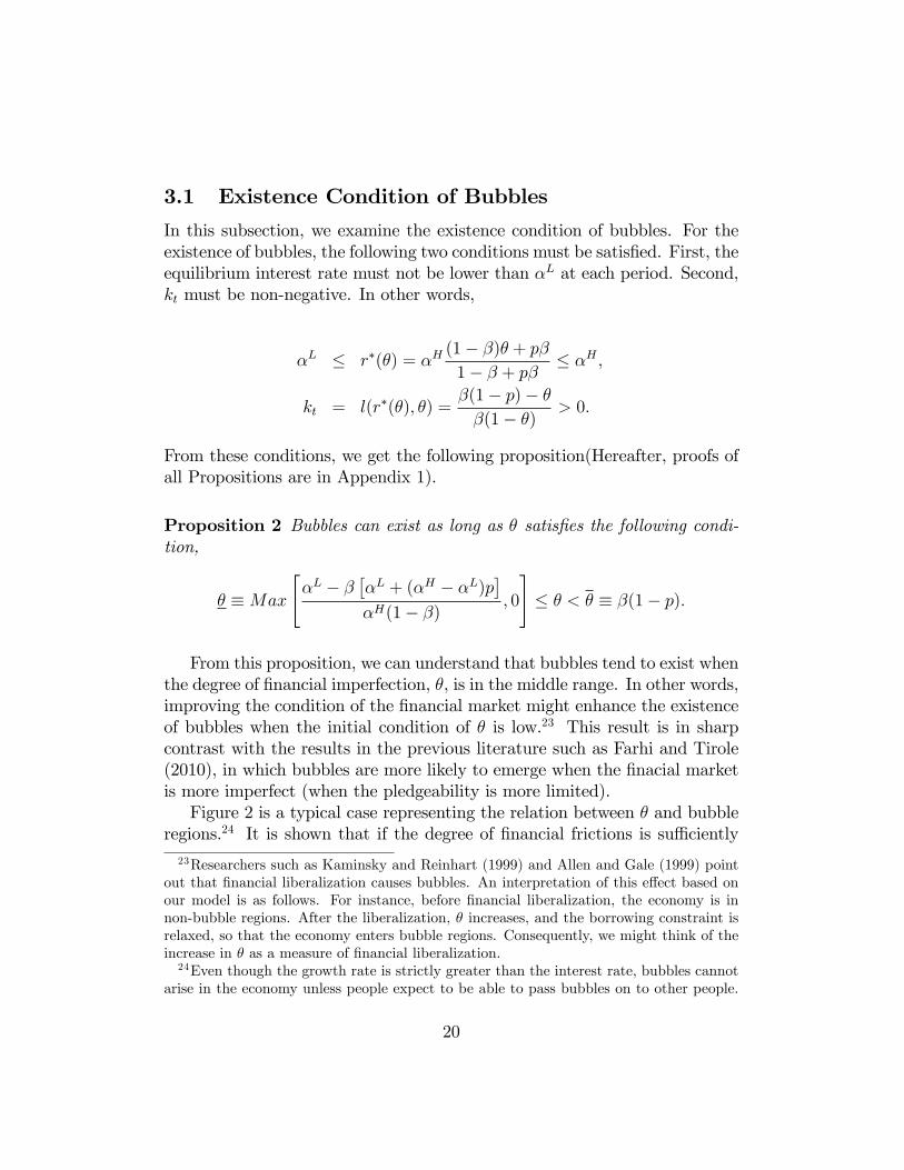
rate is equal to the rate of return on H-projects. The interest rate becomesequal to the rate of return on H-projects, and H-entrepreneurs does not facecredit constraints. The �nancial system can allocate all the savings in theeconomy to H-projects, and resource allocation is e¢ cient, even though � isstrictly less than one.16 In this region, the characteristics of the economy isthe same as the one with the perfect �nancial market.Figure 1 depicts this situation. On the horizontal axis, we take �, and

on the vertical axis, we take g and r: We show that the relation between g

16In � 2 (0; 1� p), H-entrepreneurs earn �H(1 � �)=�1� ��H=rt

�; which is strictly

greater than rt that L-entrepreneurs earn. Thus, income distribution is di¤erent betweenthe entrepreneurs. However, in � 2 [1� p; 1], both entrepreneurs earn the same rate ofreturn, which is �H : Hence, there is no di¤erence in income distribution.

14

and � is nonlinear. As shown below, this nonlinearity plays a crucial role increating regions where bubbles can arise (bubble regions), or regions wherethey cannot arise (non-bubble regions).

3 Existence of Asset Bubbles

Now we describe the economy with asset bubbles (we call this a "bubbleeconomy"). We de�ne bubble assets as the assets that produce no real return,i.e., the fundamental value of the assets is zero. Let xit be the level of bubbleassets purchased by type i entrepreneur at date t, and let Pt be the per unitprice of bubble assets at date t in terms of consumption goods. 17 In thebubble economy, each entrepreneur faces the following three constraints: �owof funds condition, the borrowing constraint, and the short-sale constraint:

c�it + z�it + Ptx

it = y

�it � r�t�1b�it�1 + b�it + Ptxit�1; (21)

r�t b�it � �(�itz�it + Pt+1xit); (22)

xit � 0; (23)

where � represents the case of bubble economy. Both sides of (21) includebubbles. Ptxit�1 in the right hand side is the sales of the bubble assets, andPtx

it in the left hand side is the new purchase of them. We de�ne the net worth

of the entrepreneur in the bubble economy as e�it � y�it � r�t�1b�it�1 + Ptxit�1:(22) is the borrowing constraint under the bubble economy. We assume herethat only a fraction � of the returns from the investment and the bubblescan be pledgeable to creditors. Of course, we can think about a di¤erentsituation in which the pledgeable fraction on the return on the investmentand that of the return on the bubbles are di¤erent. Even if we assume thatthe pledgeable fraction of bubbles�return, say �x < 1, is di¤erent from thatof the investment�s return, �, our results which will be explained below arenot a¤ected.18

We should add a few remarks about the short-sale constraint (23). AsKocherlakota (1992) has shown, the short-sale constraint is important for

17Here we only focus on deterministic bubbles but, even if we allow stochastic bubbles,our qualitative properties are not a¤ected as shown in Appendix 2.18As will be explained below, the crucial point for our results is that the previous return

from bubbles increases the net worth for a borrower.

15

the existence of bubbles in deterministic economies with a �nite number ofin�nitely lived agents. Without the constraint, bubbles always represent anarbitrage opportunity for an in�nitely lived agent; he can gain by perma-nently reducing his holdings of the asset. However, it is well known thatin such economies, equilibria can only exist if agents are constrained not toengage in Ponzi schemes. Kocherlakota (1992) has demonstrated that theshort-sale constraint is one of no-Ponzi-game conditions and hence, it cansupport bubbles by eliminating the agent�s ability to permanently reduce hisholdings of the asset.19

In order that bubble assets be held in equilibrium, the rate of return onbubbles has to be equal to the interest rate:

r�t =Pt+1Pt: (24)

Each entrepreneur chooses the levels of consumption, investment, output,borrowing, and bubble assets

�c�it ; z

�it ; y

�it+1; b

�it ; x

it

; to maximize the expected

utility (1) subject to (21), (22), and (23), given the interest rate and the cur-rent and future price of bubbles, r�t ; Pt; and Pt+1. Moreover, on the optimalfeasible plan, the following transversality condition must be satis�ed:20

lim inft!1

�t1

c�itPtx

it = 0: (25)

In equilibrium, as before, the entrepreneur consumes a fraction 1 � � ofthe net worth every period.21 As in the previous section, we focus on the casewhere the equilibrium interest rate is strictly lower than the productivity ofthe H-projects, that is, L-entrepreneurs purchase bubbles and the borrowingconstraint on H-entrepreneurs is binding. The investment function of theentrepreneurs who have H-projects at date t is

z�t =�e�it

1� ��H

r�t

:

19See Kocherlakota (1992) for details.20See Kocherlakota (1992) for the transversality condition in economies with the short

sale constraint.21The detail analysis of the maximization problem for the entrepreneur is given in Ap-

pendix.

16

where e�it = �r�t�1b�it�1+Ptxit�1 for L-H entrepreneurs, and e�it = y�it �r�t�1b�it�1for H-H entrepreneurs. For L-H entrepreneurs, since they purchased bubblesin the previous period, they are able to sell bubbles at the time they en-counter H-projects. As a result, their net worth increases (compared to thebubbleless case) and boosts their investments, that is, the "balance sheet ef-fect" works.22 Moreover, the expansion level of the investment is more thanthe direct increase of net worth because of the leverage e¤ect. H-H entrepre-neurs, however, are not able to take advantage of this merit, because theydid not buy bubbles in the previous period.Next, we describe the aggregate economy. Since both H-and L-entrepreneurs

consume a fraction 1� � of their net worth, the goods market clearing con-dition can be written as

Z�Ht + PtX = �(Y �t + PtX); (26)

where Y �t +PtX and �(Y �t +PtX) are the aggregate wealth (total asset) andthe aggregate saving in the bubble economy. X is the aggregate quantity ofbubbles, which is exogenously �xed. We see that some of the aggregate saving�ow to bubble assets as well as H-projects, which can be the source for raisingthe interest rate in the �nancial market. The aggregate demand for bubbles,PtX, is equal to the aggregate saving minus the aggregate investment ofH-entrepreneurs, �(Y �t + PtX)� Z�Ht .The aggregate investment function becomes,

Z�Ht =�E�Ht

1� ��H

r�t

;

where E�Ht = p(Y �t � r�t�1B�Ht�1) + p(PtX � r�t�1B�Lt�1) = p (Y �t + PtX). The�rst term is the aggregate net worth of H-H entrepreneurs at date t and thesecond term represents the one of L-H entrepreneurs at date t. Hence, it canbe written as

Z�Ht =�p (Y �t + PtX)

1� ��H

r�t

: (27)

22In Kiyotaki and Moore (1997), the rise in land price increases the entrepreneurs�networth, which results in balance sheet e¤ects, thereby increasing investment. In this paper,bubbles play a similar role as the land in Kiyotaki and Moore�s paper.

17

The aggregate wealth under the bubble economy can be written as,

Y �t+1 + Pt+1X = �HZ�Ht + r�tPtX: (28)

In order to characterize the economic growth rate, let us de�ne as follows,

kt =PtX

�(Y �t + PtX);

gkt =Y �t+1 + Pt+1X

Y �t + PtX;

where kt is the relative size of bubbles and gkt is the growth rate of theaggregate wealth, Y �t + PtX. From (27) and these de�nitions, (28) can bewritten as

gkt = �H �p

1� ��H

r�t

+ r�t �kt: (29)

Moreover, from (26), we get

�p

1� ��H

r�t

+ �kt = �: (30)

From (29) and (30), the growth rate of the aggregate wealth, gkt , becomes

gkt = �H�(1� kt) + r�t �kt = �H� � (�H � r�t )�kt:

Furthermore,

kt = 1�p

1� ��H

r�t

=r�t (1� p)� ��Hr�t � ��H

= l(r�t ; �): (31)

This means that given rt and �, the relative size of bubbles, kt, is just equalto the relative size of L-projects, lt = l(rt; �) under the bubbleless economy.Hence, we can derive the following growth rate function,

18

gkt (r�t ; �) = ��

H � (�H � r�t )�l(r�t ; �):This means the growth rate function in the bubble economy is just same asthe bubbleless economy. However, the growth rate becomes di¤erent sincethe equilibrium interest rate is di¤erent.Next we examine the determination process of r�t . From the de�nition of

ktkt+1kt

=rtgkt=

rt�H� � (�H � rt)�kt

: (32)

In order to satisfy the transversality condition (25),

kt+1kt

=r�tgkt� 1 (33)

should be satis�ed. Moreover, if kt+1=kt < 1, the economy converges to theasymptotically bubbleless economy. Hence, in this paper, we focus on thecase where kt+1=kt = 1, that is, the share of the bubble assets is constantunder the steady state. Hence, at each period, the following condition mustbe satis�ed:

r�(�) = �H� � (�H � r�(�))�l(r�(�); �): (34)

From (31) and kt+1=kt = 1, we get the equilibrium interest rate and therelative size of bubbles as follows,

r�t = r�(�) = �H(1� �)� + p�1� � + p� ;

kt = l(r�(�); �) =�(1� p)� ��(1� �) :

Furthermore, since the growth rate of the total output, g�t � Y �t+1=Y �t is justequal to gkt from kt+1=kt = 1, we get

g�t = gkt = r

�(�) = ��H� (�H� r�(�))�l(r�(�); �) = �H (1� �)� + p�1� � + p� : (35)

Obviously, the equilibrium growth rate is an increasing function of �. Anincrease of � decreases the relative size of bubbles, kt, and raises the growthrate.

19

3.1 Existence Condition of Bubbles

In this subsection, we examine the existence condition of bubbles. For theexistence of bubbles, the following two conditions must be satis�ed. First, theequilibrium interest rate must not be lower than �L at each period. Second,kt must be non-negative. In other words,

�L � r�(�) = �H(1� �)� + p�1� � + p� � �H ;

kt = l(r�(�); �) =�(1� p)� ��(1� �) > 0:

From these conditions, we get the following proposition(Hereafter, proofs ofall Propositions are in Appendix 1).

Proposition 2 Bubbles can exist as long as � satis�es the following condi-tion,

� �Max"�L � �

��L + (�H � �L)p

��H(1� �) ; 0

#� � < � � �(1� p):

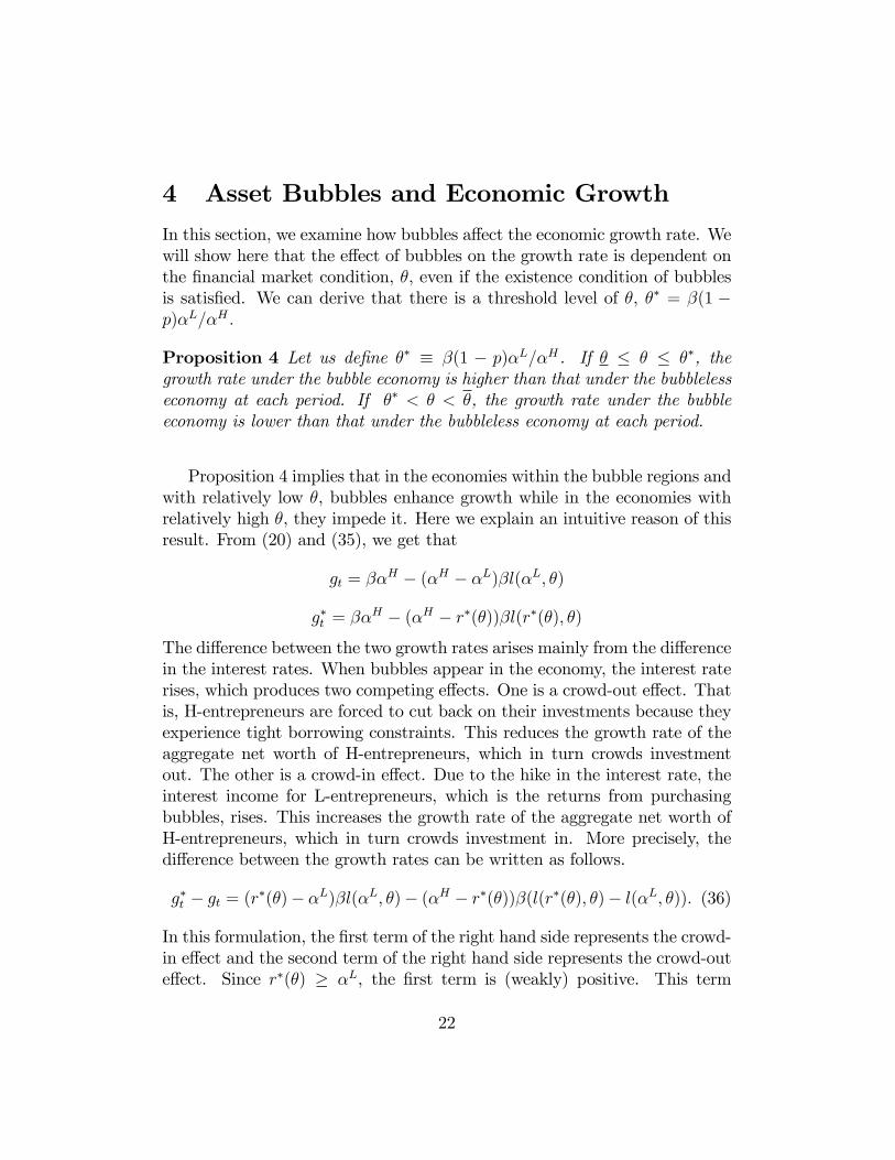
From this proposition, we can understand that bubbles tend to exist whenthe degree of �nancial imperfection, �, is in the middle range. In other words,improving the condition of the �nancial market might enhance the existenceof bubbles when the initial condition of � is low.23 This result is in sharpcontrast with the results in the previous literature such as Farhi and Tirole(2010), in which bubbles are more likely to emerge when the �nacial marketis more imperfect (when the pledgeability is more limited).Figure 2 is a typical case representing the relation between � and bubble

regions.24 It is shown that if the degree of �nancial frictions is su¢ ciently23Researchers such as Kaminsky and Reinhart (1999) and Allen and Gale (1999) point

out that �nancial liberalization causes bubbles. An interpretation of this e¤ect based onour model is as follows. For instance, before �nancial liberalization, the economy is innon-bubble regions. After the liberalization, � increases, and the borrowing constraint isrelaxed, so that the economy enters bubble regions. Consequently, we might think of theincrease in � as a measure of �nancial liberalization.24Even though the growth rate is strictly greater than the interest rate, bubbles cannot

arise in the economy unless people expect to be able to pass bubbles on to other people.

20

large or small, bubbles can not exist. This suggests that in �nancially under-developed or well-developed economies, bubbles can not emerge. They canonly arise in �nancially intermediate-developed ones.25 An intuitive reasonfor this result is as follows. If � is low, H-entrepreneurs cannot borrow suf-�ciently and the growth rate must be low even with bubbles. On the otherhand, the interest rate cannot be lower than �L; since there is an opportunityto invest in L-projects even if � is low. Hence, under a very low � level, theinterest rate becomes higher than the growth rate and bubbles cannot exist.Since we assume heterogeneous investment opportunities, the interest ratehas the lowest bound and we can obtain the result that is di¤erent from theprevious literature.26

Moreover, we can use the structure of the bubbleless economy to char-acterize the existence condition. The existence condition of the bubble isthat the growth rate is not lower than the interest rate under the bubblelesseconomy. This condition is consistent with the existence condition in theprevious literature such as Tirole(1985).

Proposition 3 The necessary condition for the existence of bubble is thatthe equilibrium growth rate is not lower than the equilibrium interest rateunder the bubbleless economy.

This expectation is the su¢ cient condition for the existence of bubbles. Here, we assumethat the condition is satis�ed when bubbles appear.25Readers may wonder why the phenomenon which looks like bubbles occurs repeatedly

in the real world where the �nancial system is continually developing over time, eventhough our model suggests that bubbles do not appear in high � regions. We proposeone interpretation from our model. In the paper, we assume a common � on both highand low investment. However, we can put di¤erent � on those projects. In such a case,the important factor for the existence of bubbles is �H ; which is placed on high-pro�tinvestments, not on low-pro�t investments. Taking this into account, consider the situationwhere the existing projects with �L disappear, and new investment opportunities withhigher pro�tability than the existing �H appear in the economy. In such a situation, the� that is placed on those new projects is important for the existence of bubbles. If the �is low, the economy will enter bubble regions again even if it was in non-bubble regionswith high � before. In the real world, this process might repeat itself.26Martin and Ventura (2010) assume two types of investment opportunities but bubbles

may be able to exist in an economy without credit markets. The crucial di¤erence is thattheir paper allows new bubble creations at each period.

21

4 Asset Bubbles and Economic Growth

In this section, we examine how bubbles a¤ect the economic growth rate. Wewill show here that the e¤ect of bubbles on the growth rate is dependent onthe �nancial market condition, �, even if the existence condition of bubblesis satis�ed. We can derive that there is a threshold level of �, �� = �(1 �p)�L=�H :

Proposition 4 Let us de�ne �� � �(1 � p)�L=�H . If � � � � ��, thegrowth rate under the bubble economy is higher than that under the bubblelesseconomy at each period. If �� < � < �, the growth rate under the bubbleeconomy is lower than that under the bubbleless economy at each period.

Proposition 4 implies that in the economies within the bubble regions andwith relatively low �, bubbles enhance growth while in the economies withrelatively high �, they impede it. Here we explain an intuitive reason of thisresult. From (20) and (35), we get that

gt = ��H � (�H � �L)�l(�L; �)

g�t = ��H � (�H � r�(�))�l(r�(�); �)

The di¤erence between the two growth rates arises mainly from the di¤erencein the interest rates. When bubbles appear in the economy, the interest raterises, which produces two competing e¤ects. One is a crowd-out e¤ect. Thatis, H-entrepreneurs are forced to cut back on their investments because theyexperience tight borrowing constraints. This reduces the growth rate of theaggregate net worth of H-entrepreneurs, which in turn crowds investmentout. The other is a crowd-in e¤ect. Due to the hike in the interest rate, theinterest income for L-entrepreneurs, which is the returns from purchasingbubbles, rises. This increases the growth rate of the aggregate net worth ofH-entrepreneurs, which in turn crowds investment in. More precisely, thedi¤erence between the growth rates can be written as follows.

g�t � gt = (r�(�)� �L)�l(�L; �)� (�H � r�(�))�(l(r�(�); �)� l(�L; �)): (36)

In this formulation, the �rst term of the right hand side represents the crowd-in e¤ect and the second term of the right hand side represents the crowd-oute¤ect. Since r�(�) � �L, the �rst term is (weakly) positive. This term

22

captures the e¤ect that an increase in the interest rate raises the income ofthe entrepreneurs who invested in the bubbles and enhances the economicgrowth rate. More precisely, if there is no bubble, some L-entrepreneurs haveto invest in L-projects, l(�L; �), as long as the borrowing constraint binds theH-entrepreneurs. If they have a chance to invest in bubble assets instead ofL-projects, they can earn r�(�)l(�L; �) instead of �Ll(�L; �). This increasedearning contributes to enhancing the H-investment at the time they becomeH-entrepreneurs in the future. Thus, this income e¤ect increases the growthrate by the increase of H-investments.The second term represents the crowd-out e¤ect. As you can see from

(17), l(r�; �) is an increasing function of r�. A rise in the interest rate tightensthe borrowing constraint of the H-entrepreneuers and increases the invest-ments in the L-projects or bubbles. Hence, l(r�(�); �) � l(�L; �) is positive.Under the bubble economy, if � is low, �l(�L; �) is high and the crowd-ine¤ect is high. On the other hand, if � is high, �l(�L; �) becomes low and thecrowd-in e¤ect is dominated by the crowd-out e¤ect. Thus, in the economieswith relatively low �, the crowd-in e¤ect dominates the crowd-out e¤ect, but,in the economies with relatively high �, the crowd-out e¤ect dominates thecrowd-in e¤ect.27

Here, we will add a few remarks on the e¤ect of bubbles on aggregateproductivity. In the bubble economy, L-entrepreneurs stop investing andonly H-entrepreneurs invest, i.e., bubbles improve e¢ ciency in production byeliminating low-productive investments. Thus, the total factor productivityincreases together with the emergence of bubbles. It moves procyclically witheconomic growth if � is relatively low. This implies that bubble bursts resultsin productive ine¢ ciency.

5 E¤ects of the Bubbles Bursting

In this section, we examine the e¤ects of bubble bursts. In this perfectforesight model, an unexpected shock may generate a burst of bubbles.28

27In our model, the presence of L-projects plays a crucial role in showing that bubblescrowd investment in and enhance growth. Without them, in the bubbleless economy, theinterest rate adjusts such that all the savings in the economy �ow to H-projects. In sucha situation, once bubble assets appear in the economy, they crowd savings away fromH-projects, thereby lowering the growth.28When we assume stochastic bubbles, bubbles can burst even without exogenous shocks.

The e¤ects of bubbles bursting are examined in Appendix 2 and we can show that qual-

23

Let us suppose that there is an unexpected shock at t = s that decreases theproductivity from �H to �S < �H . First, we examine the case where thisshock is permanent (or at least this shock is expected to be permanent att = s.). As we have shown in the previous section, ��H � �L is a necessarycondition for the existence of bubbles. Hence, if �S is strictly smaller than�L=�, bubbles must burst for any �. Even if �S � �L=�, bubbles may burstif � is relatively low. Since � is a decreasing function of �H , bubbles mustcollapse in the countries whose pledgeability is lower than �(�S). This resultshows that even if the shock is common, the e¤ect of the shock di¤ers fromcountry to country and in particular, the e¤ect on the stock price in a countryis crucially a¤ected by the �nancial market conditions of this country.Next, we examine how the growth rate in each country is a¤ected by the

unexpected shock at t = s. After the collapse of bubbles, the growth rateis determined by the mechanism explained in Section 2. Hence, the growthrate after the shock becomes,

gt = g(�) =

8>>><>>>:��S � (�S � �L)��

L(1� p)� ��S�L � ��S if 0 � � < (1� p)�

L

�S;

��S; if (1� p)�L

�S� � � 1:

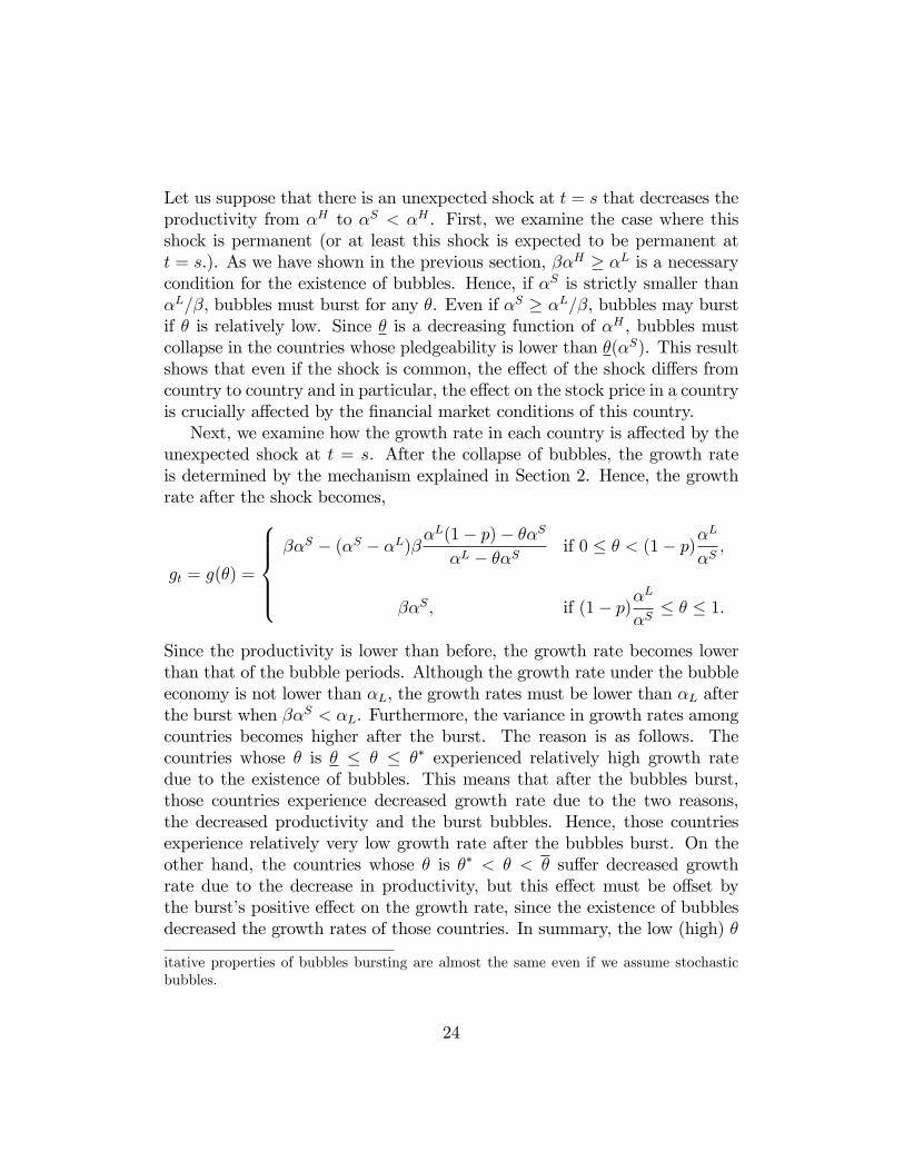
Since the productivity is lower than before, the growth rate becomes lowerthan that of the bubble periods. Although the growth rate under the bubbleeconomy is not lower than �L, the growth rates must be lower than �L afterthe burst when ��S < �L. Furthermore, the variance in growth rates amongcountries becomes higher after the burst. The reason is as follows. Thecountries whose � is � � � � �� experienced relatively high growth ratedue to the existence of bubbles. This means that after the bubbles burst,those countries experience decreased growth rate due to the two reasons,the decreased productivity and the burst bubbles. Hence, those countriesexperience relatively very low growth rate after the bubbles burst. On theother hand, the countries whose � is �� < � < � su¤er decreased growthrate due to the decrease in productivity, but this e¤ect must be o¤set bythe burst�s positive e¤ect on the growth rate, since the existence of bubblesdecreased the growth rates of those countries. In summary, the low (high) �

itative properties of bubbles bursting are almost the same even if we assume stochasticbubbles.

24

countries experience relatively lower (higher) growth rates; thus the variancein growth rate becomes higher even though the average growth rate must belower than before the burst. This result may be consistent with an empiricalobservation. Figure 3 shows the growth rates of Asian countries before andafter the �nancial crisis. The �gure shows that the variance in the growthrates becomes higher after the crisis. Although, actual growth rates will bea¤ected by many factors, our result is not inconsistent with this interestingobservation.Next we examine the case where the unexpected shock is temporary and

it is expected to be so after the shock. In this case, bubbles might existeven after the shock since all agents can expect that this shock is temporary.In order to sustain the bubble path after the shock, however, the price ofbubbles, Ps; must drop according to the shock. The reason is as follows. Letus suppose the shock is temporary and that the productivity recovers to �H

after t = s + 1. Under the shock, from t = s + 1, the growth rate of eachcountry can recover to g�t (�) but Yt must be lower since Ys+1 is decreased bythe shock. Hence, in order to sustain the bubble path, the price of bubblesmust decrease at t = s. This result suggests that the decrease in asset pricesdoes not directly mean that the bubbles burst. It might be the adjustmentprocess of bubbles. Even after the drop in asset prices, bubbles can existeven under the perfect foresight economy as long as there is an unexpectedshock.It is not necessary, however, that people continue to choose the bubble

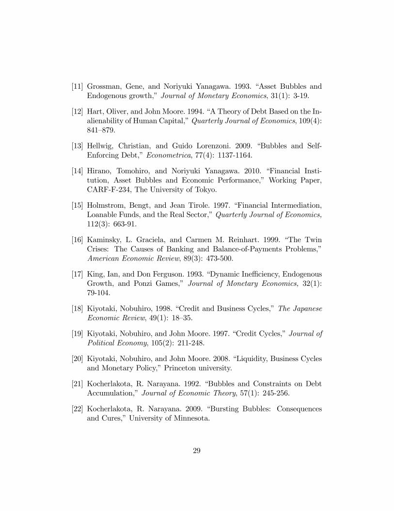
path even after the unexpected shock. People may choose the bubbleless pathafter the shock. Hence, bubbles may burst if agents revise their expectationas a result of the shock and expect that the value of the bubble is zero evenif the productivity shock is temporary and �H recovers to the original levelat t = s + 1. Next, we examine how the bubble bursts a¤ect the economicgrowth rates in this case. Since the bubbles have burst at t = s, the growthrate follows (20) from t = s + 1. This implies that the di¤erence betweenthe growth rates before and after the bubbles burst can be characterizedby the di¤erence between the growth rates of the bubble economy and thebubbleless economy. Hence, if � � � � ��, the growth rate becomes lowerafter the bubbles burst but if �� < � < �, the growth rate becomes higher(except t = s) after the bubbles burst.29 This result suggests that the e¤ect of

29In the standard real business cycle models, a temporary productivity shock has onlytemporal e¤ects on output. However, in our model, even a small temporary shock on

25

bubble bursts is not uniform. It is crucially a¤ected by the �nancial conditionof each country. If the imperfection of the �nancial market is relatively high,the bursting of bubbles decreases the growth rate of the country but thebursts may enhance the long run growth rate if the condition of the �nancialmarket is relatively good. This point is shown in Figure 4.30 In other words,the bubbles bursting explores the "true" economic condition of each country.This result also means that the variance in growth rates among countriesbecomes higher and, once again, this result is consistent with the observationin Figure 3.

6 Conclusion

In this paper, we assumed the imperfection of the �nancial markets and ex-amined the e¤ects of bubbles under the imperfect �nancial market condition.We explored how the existence condition of bubbles is related to the condi-tion of the �nancial market and how the middle range of pledgeability allowsfor the existence of bubbles. This suggests that improving the condition ofthe �nancial market might enhance the possibility of bubbles if the initialcondition of the �nancial market is underdeveloped.31 Moreover, the e¤ectsof bubbles on the economic growth rates are also related to the �nancialmarket�s condition. If the pledgeability is relatively low, bubbles increasethe growth rate; but bubbles decrease the growth rate if the pledgeability isrelatively high. This result has an important implication for the e¤ects ofbubble bursts. The bursting of the bubbles decreases the growth rate when

productivity of the entrepreneurs�investment has permanent e¤ects on the aggregate pro-ductivity and the long run growth rate.30If � � � � ��; the growth rate at t = s might be higher than t = s�1 if the temporary

shock is not so large since the growth rate is enhanced by the burst of bubbles even att = s.31In our model, the volatility of the growth rate is high when � is in the middle range,

because bubbles can occur. This may be consistent with the empirical evidences such asEasterly et al. (2000), and Kunieda (2008), which shows that macroeconomic volatility ishigh when �nancial development is an intermediated level. As theoretical papers, thereare Aghion et al. (1999), and Matsuyama (2007, 2008), in which they show that macroeco-nomic volatility is high when the �nancial market is intermediatedly developed. However,the source of high volatility is di¤erent between these papers and ours. In our paper, it isfrom the appearance of bubbles, while in their papers, it comes from the interest rate orquality of investments.

26

the condition of the �nancial market is not so good, but the bursts mayenhance the growth rate when the �nancial market�s condition is relativelygood. These imply that the bubbles bursting explores the "true" economiccondition of each country. In order to sustain high long-run growth rates,realizing the high quality of the �nancial system is important.Our model could be extended in several directions. One direction would

be to endogenize the pledgeability. In this model, we assume that the levelof the pledgeability is exogenously given. It would be interesting to examinehow the pledgeability is a¤ected by legal systems or behaviors of �nancialsectors and how these factors a¤ect the bubble regions. Another directionwould be to extend our model into a two-countries model with di¤erentpledgeability levels, and investigate how globalization such as capital accountliberalization a¤ects the emergence of bubbles in each country. Finally, wehave not analyzed the welfare implications of bubbles, policy-oriented issuessuch as government�s intervention after bubble bursts, or the role of �nancialmarket regulations on the emergence of bubbles. These would be promisingareas for future research.32

32Lorenzoni (2008) presents an interesting framework to study policies in the presence ofpecuniary externality which comes from ampli�cation in asset prices. Analyzing bubbleswithin Lorenzoni�s framework will be interesting research for understanding regulationswhich prevent bubbles or government�s intervention after bursts of bubbles.

27

References

[1] Akerlof, George, and Robert Shiller. 2009. Animal Spirits. How HumanPsychology Drives the Economy and Why It Matters for Global Capi-talism. Princeton, New Jersey: Princeton University Press.

[2] Aoki, Kosuke, and Kalin Nikolov. 2010. �Bubbles, Banks and FinancialStability,�mimeo, Bank of Japan.

[3] Aghion, Philippe, Abhijit Banerjee, and Thomas Piketty. 1999. �Du-alism and Macroeconomic Volatility.�The Quarteryly Journal of Eco-nomics, 114(4): 1359-97.

[4] Bernanke, Ben, and Mark Gertler. 1989. �Agency Costs, Net Worth,and Business Fluctuations,�American Economic Review, 79(1): 14�31.

[5] Bernanke, Ben, Mark Gerlter, and Simon Gilchrist. 1999. �The FinancialAccelerator in a Quantitative Business Cycle Framework,�in J. Taylorand M. Woodford eds, the Handbook of Macroeconomics, 1341-1393.Amsterdam: North-Holland.

[6] Caballero, Ricardo. 2006. �On the Macroeconomics of Asset Shortages,�The Role of Money: Money and Monetary Policy in the Twenty-FirstCentury The Fourth European Central Banking Conference 9-10 No-vember 2006, Andreas Beyer and Lucrezia Reichlin, editors, 272-283.

[7] Caballero, Ricardo, and Arvind Krishnamurthy. 2006. �Bubbles andCapital Flow Volatility: Causes and Risk Management,� Journal ofMonetary Economics, 53(1): 35-53.

[8] Easterly, R. Easterly, Roumeen Islam, and Joseph Stiglitz. 2000.�Shaken and Stirred: Explaining Growth Volatility,� In Annual BankConference on Development Economics 2000, edited by Boris Pleskovicand Nicholas Stern, Washington, DC: The World Bank.

[9] Farhi, Emmanuel, and Jean Tirole. 2011. �Bubbly Liquidity,�forthcom-ing in Review of Economic Studies.

[10] Gertler, Mark, and Nobuhiro Kiyotaki. 2010. �Financial Intermediationand Credit Policy in Business Cycle Analysis,�New York University.

28

[11] Grossman, Gene, and Noriyuki Yanagawa. 1993. �Asset Bubbles andEndogenous growth,�Journal of Monetary Economics, 31(1): 3-19.

[12] Hart, Oliver, and John Moore. 1994. �A Theory of Debt Based on the In-alienability of Human Capital,�Quarterly Journal of Economics, 109(4):841�879.

[13] Hellwig, Christian, and Guido Lorenzoni. 2009. �Bubbles and Self-Enforcing Debt,�Econometrica, 77(4): 1137-1164.

[14] Hirano, Tomohiro, and Noriyuki Yanagawa. 2010. �Financial Insti-tution, Asset Bubbles and Economic Performance,� Working Paper,CARF-F-234, The University of Tokyo.

[15] Holmstrom, Bengt, and Jean Tirole. 1997. �Financial Intermediation,Loanable Funds, and the Real Sector,�Quarterly Journal of Economics,112(3): 663-91.

[16] Kaminsky, L. Graciela, and Carmen M. Reinhart. 1999. �The TwinCrises: The Causes of Banking and Balance-of-Payments Problems,�American Economic Review, 89(3): 473-500.

[17] King, Ian, and Don Ferguson. 1993. �Dynamic Ine¢ ciency, EndogenousGrowth, and Ponzi Games,� Journal of Monetary Economics, 32(1):79-104.

[18] Kiyotaki, Nobuhiro, 1998. �Credit and Business Cycles,�The JapaneseEconomic Review, 49(1): 18�35.

[19] Kiyotaki, Nobuhiro, and John Moore. 1997. �Credit Cycles,�Journal ofPolitical Economy, 105(2): 211-248.

[20] Kiyotaki, Nobuhiro, and John Moore. 2008. �Liquidity, Business Cyclesand Monetary Policy,�Princeton university.

[21] Kocherlakota, R. Narayana. 1992. �Bubbles and Constraints on DebtAccumulation,�Journal of Economic Theory, 57(1): 245-256.

[22] Kocherlakota, R. Narayana. 2009. �Bursting Bubbles: Consequencesand Cures,�University of Minnesota.

29

[23] Kunieda, Takuma. 2008. �Financial Development and Volatility ofGrowth Rates: New Evidence,�MPRA Paper.

[24] Lorenzoni, Guido. 2008. �Ine¢ cient Credit Booms,�Review of EconomicStudies, 75(3): 809-833.

[25] Martin, Alberto, and Jaume Ventura. 2011a. �Theoretical Notes on Bub-bles and the Current Crisis,�Forthcoming in IMF Economic Review.

[26] Martin, Alberto, and Jaume Ventura. 2011b. �Economic Growth withBubbles,�Universitat Pompeu Fabra.

[27] Matsuyama, Kiminori. 2007. �Credit Traps and Credit Cycles,�Ameri-can Economic Review, 97(1): 503-516.

[28] Matsuyama, Kiminori. 2008. �Aggregate Implications of Credit MarketImperfections,� in D. Acemoglu, K. Rogo¤, and M. Woodford, eds.,NBER Macroeconomics Annual 2007, 1-60. University of Chicago Press.

[29] Miao, Jianjun, and Pengfei Wang. 2011. �Bubbles and Credit Con-straints,�mimeo, Boston University.

[30] Olivier, Jacques. 2000. �Growth-Enhancing Bubbles,� InternationalEconomic Review, 41(1): 133-51.

[31] Sakuragawa, Masaya. 2010. �Bubble Cycles,�mimeo, Keio University.

[32] Samuelson, Paul. 1958. �An Exact Consumption-Loan Model of Interestwith or without the Social Contrivance of Money,�Journal of PoliticalEconomy, 66(6): 467-482.

[33] Santos, S. Manuel, andMichael Woodford. 1997. �Rational Asset PricingBubbles,�Econometrica, 65(1): 19-58.

[34] Saint G. Paul. 1992. �Fiscal Policy in an Endogenous Growth Model,�Quarterly Journal of Economics, 107(4): 1243-1260.

[35] Scheinkman, A. Jose, and LaurenceWeiss. 1986. �Borrowing Constraintsand Aggregate Economic Activity,�Econometrica, 54(1): 23-45.

[36] Tirole, Jean. 1982. �On the Possibility of Speculation under RationalExpectations,�Econometrica, 50(5): 1163-1182.

30

[37] Tirole, Jean. 1985. �Asset Bubbles and Overlapping Generations,�Econometrica, 53(6): 1499-1528.

[38] Tirole, Jean. 2005. The Theory of Corporate Finance. Princeton, NewJersey: Princeton University Press.

[39] Wang, Pengfei, and Yi Wen. 2009. �Speculative Bubbles and FinancialCrisis.�Working Paper No. 2009-029, Federal Reserve Bank of St. Louis.

[40] Woodford, Michael. 1990. �Public Debt as Private Liquidity,�AmericanEconomic Review, 80(2): 382-388.

31

g, r

N o n ­B ub ble B u bb le N on ­B u bb le

                            R e g ion R egio n   R eg io n

0 1 θ

F igu re 1: B u bb le  reg ion  an dθ

α H

α L

g

r

g, g*

g*

g

Non­Bubble

Non­Bubble Bubble Region Region

Region

0               1 θ

Figure 2: Bubbles and Economic Growth

βαH

αL

32

­20

­15

­10

­5

0

5

10

15

1Q 2Q 3Q 4Q 1Q 2Q 3Q 4Q 1Q 2Q 3Q

2007 2008 2009

India

Hong Kong

Korea

Singapore

Thailand

Malaysia

Philippines

Indonesia

Vietnam

%

Thomson Reuter, Datastream* year­over­year basis

Figure 3: Real GDP Quarterly Growth

33

s­1                s       s+1 t

Figure 4­1: The effect of bubbles’ bursting in relatively lowθ

Effects caused by the decline in αH

Effects caused bybubble burst Growth rate after bubble burst

Growth rate before bubble burst

Growth rate after bubble bursts

Growth rate beforebubble burst

s­1                s           s+1 t

Figure 4­2: The effects of bubbles’ bursting in relatively highθ

Effects caused by the decline in αH

Effects caused by bubble burst

34

Appendix 1

Maximization Problem for the entrepreneur in the bub-bleless economy

We derive the �rst order conditions of this problem by solving the Lagrangian(L)

Li0 = E01Xt=0

�t�log(�it�1z

it�1 � rt�1bit�1 + bit � zit) + �it(��itzit � rtbit) + �itzit

�;

where �it; �it are Lagrange multipliers on the borrowing constraint and non-

negative constraint (zit � 0), respectively.First order conditions:

@Lit@zit

= � 1cit+ �it��

it + �

it + Et

���itcit+1

�= 0;

@Lit@bit

=1

cit� �itrt � Et

��rtcit+1

�= 0:

Complementary slackness condition:

�it � 0; rtbit � ��itzit; �it(��itzit � rtbit) = 0;

�it � 0; zit � 0; �itzit = 0:

Then we obtain

If �it > rt; �it > 0 and �

it = 0;

If �it = rt; �it = 0 and �

it = 0;

If �it < rt; �it = 0 and �

it > 0:

35

Maximization Problem for the entrepreneur in the bub-ble economy

We derive the �rst order conditions of this problem by solving the Lagrangian(L)

L�i0 = E01Xt=0

�t�log(�it�1z

�it�1 � r�t�1b�it�1 + b�it � z�it ) + ��it (��itz�it � r�t b�it ) + ��it Ptxit + ��it z�it

�;

where ��it ; ��it ; �

�it are Lagrange multipliers on the borrowing constraint, the

short sale constraint, and non-negative constraint (z�it � 0), respectively.First order conditions:

@L�it@z�it

= � 1

c�it+ ��it ��

it + �

�it + Et

���itc�it+1

�= 0;

@L�it@b�it

=1

c�it� ��it rt � Et

��r�itc�it+1

�= 0;

@L�it@Ptxit

= � 1

c�it+ ��it �

Pt+1Pt

+ ��it + Et

��1

c�it+1

Pt+1Pt

�= 0:

Complementary slackness condition:

��it � 0; r�t b�it � �(�itz�it + Pt+1xit); ��it

��(�itz

�it + Pt+1x

it)� r�t b�it

�= 0;

��it � 0; xit � 0; ��it xit = 0;��it � 0; z�it � 0; ��it z�it = 0:

Then we obtain

If �it > r�it ; �

�it > 0; �

�it > 0 and �

�it = 0;

If �it = r�it ; �

�it = 0; �

�it = 0 and �

�it = 0;

If �it < r�it ; �

�it = 0; �

�it = 0 and �

�it > 0:

Proof of Proposition 2

If ��H < �L, the growth rate of this economy cannot be equal to the interestrate and bubbles cannot exist. This situation is the case where > �(1 � p)and � which satis�es the above condition does not exist. Thus, we focus on

36

the cases where ��H � �L. When �L��f�L+(�H��L)pg�H(1��) > 0, r�(�) = �L and

l(r�(�); �) > 0. Since r�(�) is a strictly increasing function of �, r�(�) < �L

and bubbles cannot exist if � < � = �L��f�L+(�H��L)pg�H(1��) . On the other hand,

r�(�) � �L if � � � = �L��f�L+(�H��L)pg�H(1��) . When �L��f�L+(�H��L)pg

�H(1��) � 0, � =0 and r�(0) � �L. But � cannot be negative. Hence, we do not have toconsider the case of � < � and r�(0) � �L as long as � � � = 0. However,l(r�(�); �) is a decreasing function of � and l(r�(�); �) becomes zero when� = �(1� p) = �. Therefore, bubbles can exist as long as � � � < �.33

Proof of Proposition 3

If ��H < �L, bubbles cannot exist as explained in the proposition 1, andthe growth rate under the bubbleless economy is lower than the interestrate under the bubbleless economy for any �: Next we check the case where��H � �L. From the de�nition of �, the following relation is satis�ed.

��H � (�H � �L)�l�(�L; �) = �L:

This relation means that at �, the growth rate under the bubbleless economy(the left hand side) is equal to the interest rate under the bubbleless economy(the right hand side). When � is a little higher than � but smaller than(1�p)�L=�H , the growth rate under the bubbleless economy becomes higherthan �L but the interest rate is still �L. Thus, the growth rate is higher thanthe interest rate under the bubbleless economy. If � becomes higher than(1�p)�L=�H , the interest rate becomes ��H=(1�p) which is higher than �Land the growth rate becomes ��H . Hence, the growth rate becomes lowerthan the interest rate when � becomes higher than � � �(1�p). In summary,the growth rate is higher than the interest rate under the bubbleless economywhen � � � � �, and � � � � � is exactly the necessary condition of existenceof bubbles.33At � =

��L � �

��L + (�H � �L)p

�=��H(1� �)

�; the interest rate, the rate of re-

turn on L-projects and bubbles are the same. Thus, L-entrepreneurs invest in their ownL-projects as well as buy bubbles and lend to H-entrepreneurs.

37

Proof of Proposition 4

From (18) and (35), gt = g(�) = ��H � (�H � �L)� �L(1�p)���H�L���H , and g�t =

r�(�) = �H (1��)�+p�1��+p� . We derive � which satis�es gt = g

�t , that is

�2 � �p��H + �L(1� �) + ��L(1� � + p�)

�H(1� �) �

+�p��L +

��L + (�H � �L)p

���L

�H(1� � + p�)

�H(1� �) = 0:

(A1)

By solving the above quadratic function (A1), we can derive that

� =

��L � �

��L + (�H � �L)p

��H(1� �) ;

�� =�L

�H�(1� p):

Furthermore, from the quadratic function (A1), we can derive that gt < g�tif � < ��, and gt > g�t if � > �

�.

Appendix 2: Stochastic Bubbles

This appendix presents stochastic bubbles version of the basic model of Sec-tion 3. Following Weil (1987), we assume that bubble price becomes zero(bubble bursts) with probability 1� � at date t conditional on positive bub-ble price at date t � 1; and once they burst, they never arise again. Thisimplies that bubbles continue with probability �(< 1) and their prices arepositive until they switch to being equal to zero forever. Let Pt be the perunit price of bubble assets at date t in terms of consumption goods whenbubbles do not collapse at date t.The maximization problem for an entrepreneur is as follows:

Maxfc�it ; z�it ; b�it ; xitg1t=0

E0�P1

t=0 �t log c�it

�c�it + z

�it + Ptx

it = y

�it � r�t�1b�it�1 + b�it + Ptxit�1;

38

r�t b�it � �(�itz�it + Et

h~Pt+1x

it

i);

xit � 0;

lim inft!1

�t1

c�itPtx

it = 0;

where ~Pt+1 is a random variable, because bubbles collapse stochastically. Asbefore, we assume that only a fraction � of the returns from the investmentand the expected return on bubbles can be pledgeable to the creditors.H-entrepreneurs act much like they do in the deterministic case. On the

other hand, for L-entrepreneurs, their portfolio problem is more complicatedthan in the deterministic case. Since bubble assets deliver no return withprobability 1 � �, hence L-entrepreneurs may want to hedge themselves byinvesting in their L-projects.For date t L-entrepreneurs, from the �rst order conditions,

1

c�it= ��

r�tc�i;�t+1

+ (1� �)� r�tc�i;1��t+1

; (A2)

1

c�it= ��

1

c�i;�t+1

Pt+1Pt; (A3)

where ci;�t+1 and ci;1��t+1 are the consumption level at date t + 1 when bubbles

continue and collapse at date t+ 1; respectively.From (A2) and (A3),

�(Pt+1Pt

� r�t )c�i;1��t+1 = (1� �)r�t c

�i;�t+1 : (A4)

The aggregate counterpart to (A4) is

�(Pt+1Pt

� r�t )C�1��t+1 = (1� �)r�tC��t+1; (A5)

where C��t+1 = (1��)(�LZ�Lt �r�tB�Lt +Pt+1X) and C�1��t+1 = (1��)(�LZ�Lt �r�tB

�Lt ): Note that if r

�t = �

L; Z�Lt � 0 and if r�t > �L; Z�Lt = 0:Rearranging (A5) by using the aggregate �ow of funds constraint of date

t L-entrepreneurs, PtX + Z�Lt +B�Ht = �E�Lt ,

39

kt =

8>><>>:(�

Pt+1Pt

��L)(1�p)

(Pt+1Pt

��L)if r�t = �

L

(�Pt+1Pt

�r�t )(1�p)

(Pt+1Pt

�r�t )if r�t > �

L

: (A6)

Evolution of the aggregate wealth�s growth rate follows

gkt =

8>>><>>>:�H �p

1� ��H

�L

+ �L�� � �p

1� ��H

�L

�+ (Pt+1

Pt� �L)�kt if r�t = �

L

�H �p

1� ��H

r�t

+ Pt+1Pt

"� � �p

1� ��H

r�t

#if r�t > �

L

: (A7)

When r�t > �L; the interest rate is determined by equation (30), givenkt :

p

1� ��H

r�t

+ kt = 1: (A8)

Existence of Stochastic Bubbles

Here following Farhi and Tirole (2010), we restrict our attention to an equi-libria where the variables (gkt ; g

�t ; r

�t ;Pt+1Pt; kt) are constant over time, which

Farhi and Tirole call a conditional bubbly steady state. In this equilibria,wealth�s growth rate, output�s growth rate, the interest rate, the rate ofreturn on bubbles, and bubble share are constant until the bubbles crash.In such a conditional bubbly steady state,

gk = g� =Pt+1Pt: (A9)

From (A6)-(A9), we can obtain the conditional bubbly steady state: Inorder that the conditional bubbly steady state can exist, the following con-ditions must be satis�ed:

k > 0; (A10)

40

Z�Lt�(Y �t +PtX)

> 0 if r�t = �L: (A11)

From (A10) and (A11), we can obtain the existence condition of theconditional bubbly steady state.

Proposition 5 The existence condition of the conditional bubbly steady statebecomes

Max

"�L � �

��L + (�H � �L)p

��

�H(1� ��) ; 0

#< � < ��(1� p):

Compared to the existence condition of deterministic bubbles (Proposi-tion 2), the condition becomes tightened.Here we should note two things. The �rst one is that if

�L � ���L + (�H � �L)p

��

�H(1� ��) < 0;

then, even if � = 0; the conditional bubbly steady state can exist.The second one is that if

�H

�L<1

��;

then, the conditional bubbly steady state can not exist.Moreover, within the bubble regions, growth e¤ects of stochastic bubbles

become di¤erent depending upon �:

Proposition 6 If Max��L��[�L+(�H��L)p]�

�H(1���) ; 0

�< � � �1; the growth rate

under the stochastic bubble economy is higher than that under the bubblelesseconomy. If �1 < � < ��(1� p); the growth rate under the stochastic bubbleeconomy is lower than that under the bubbleless economy. �1 is the greatervalue of the following quadratic equation: �H �[1��(1�p)]+(1��)�

1���(1�p) = �H �L�p�L���H +

�L(� � �L�p�L���H ):

41