c© 2017 by Bryan Medaris Kerns. All rights reserved.

A MEASUREMENT OF THE x DEPENDENT SEA FLAVOR ASYMMETRY ATSEAQUEST

BY

BRYAN MEDARIS KERNS

DISSERTATION

Submitted in partial fulfillment of the requirementsfor the degree of Doctor of Philosophy in Physics

in the Graduate College of theUniversity of Illinois at Urbana-Champaign, 2017

Urbana, Illinois

Doctoral Committee:

Professor Matthias Gross Perdekamp, ChairProfessor Naomi C. R. Makins, Director of ResearchProfessor Aida X El-KhadraProfessor Peter Abbamonte

Abstract

SeaQuest is a fixed target forward spectrometer experiment located at Fermilab which uses a 120 GeV

proton beam on liquid hydrogen, liquid deuterium, and several solid targets. The flagship measurement

of this experiment is to use the Drell-Yan process to improve the accuracy of the antiquark PDFs in the

parton momentum fraction x range 0.1 to 0.58. By measuring the cross section ratio of σpd(x)/σpp(x) one

can derive an estimate of the proton sea flavor asymmetry, d/u, as a function of x.

This measurement is of interest to many theoreticians who have proposed several different classes of

models in order to simulate the inner workings of the proton, a good test of these models is how well they

predict the sea flavor asymmetry. A measurement from a previous experiment, E866, measured d < u at x

above 0.3. The models proposed so far do not predict d < u at any x, so the accuracy of the E866 experiment

in this region is of great interest.

An analysis of some but not all of the data collected by SeaQuest is presented in this paper. It contains a

measurement of σpd(x)/σpp(x), the application of several corrections and uncertainties to this measurement,

and the derivation of d(x)/u(x) from this measurement. Major corrections and uncertainties are the rate

dependence correction and the target contamination correction. Particular care is paid to how to correctly

merge the results from multiple data sets and optimizing the accuracy of estimating the value of parton

momentum fraction x from measured quantities. The most notable feature of these results is that d/u is not

less than one at any value of x, and is above one by several σ where E866 measured d/u below one.

ii

Acknowledgments

This research would not have been possible without the support of the National Science Foundation, via

grant No. 1506416.

I would like to thank my advisor, Naomi Makins, for sharing her enthusiasm for physics, which is what

first drew me to her group. I would like to offer my thanks to the professionals in the McKinley Mental

Health department, without which it is possible my anxiety and depression would have prevented me from

completing this thesis. I would also like to thank the physics department at the University of Illinois,

Urbana-Champaign, for not kicking me to the curb when I took much longer than usual to complete my

degree requirements.

iii

Table of Contents

List of Figures . . . . . . . . . . . . . . . . . . . . . . . . . . . . . . . . . . . . . . . . . . . . . . vi

List of Tables . . . . . . . . . . . . . . . . . . . . . . . . . . . . . . . . . . . . . . . . . . . . . . x

Chapter 1 Background . . . . . . . . . . . . . . . . . . . . . . . . . . . . . . . . . . . . . . . . 11.1 Proton Structure . . . . . . . . . . . . . . . . . . . . . . . . . . . . . . . . . . . . . . . . . . . 11.2 Deep Inelastic Scattering . . . . . . . . . . . . . . . . . . . . . . . . . . . . . . . . . . . . . . . 31.3 Drell-Yan Process . . . . . . . . . . . . . . . . . . . . . . . . . . . . . . . . . . . . . . . . . . . 51.4 Gottfried Sum Rule . . . . . . . . . . . . . . . . . . . . . . . . . . . . . . . . . . . . . . . . . 81.5 Sea Flavor Asymmetry in Past Experiments . . . . . . . . . . . . . . . . . . . . . . . . . . . . 10

1.5.1 New Muon Collaboration . . . . . . . . . . . . . . . . . . . . . . . . . . . . . . . . . . 101.5.2 NA51 . . . . . . . . . . . . . . . . . . . . . . . . . . . . . . . . . . . . . . . . . . . . . 101.5.3 E866/NuSea . . . . . . . . . . . . . . . . . . . . . . . . . . . . . . . . . . . . . . . . . 12

1.6 Motivation . . . . . . . . . . . . . . . . . . . . . . . . . . . . . . . . . . . . . . . . . . . . . . 131.7 Models . . . . . . . . . . . . . . . . . . . . . . . . . . . . . . . . . . . . . . . . . . . . . . . . . 16

Chapter 2 Experimental Setup . . . . . . . . . . . . . . . . . . . . . . . . . . . . . . . . . . . 212.1 Timeline . . . . . . . . . . . . . . . . . . . . . . . . . . . . . . . . . . . . . . . . . . . . . . . . 222.2 Beam . . . . . . . . . . . . . . . . . . . . . . . . . . . . . . . . . . . . . . . . . . . . . . . . . 232.3 Targets . . . . . . . . . . . . . . . . . . . . . . . . . . . . . . . . . . . . . . . . . . . . . . . . 272.4 Magnets . . . . . . . . . . . . . . . . . . . . . . . . . . . . . . . . . . . . . . . . . . . . . . . . 322.5 Detectors . . . . . . . . . . . . . . . . . . . . . . . . . . . . . . . . . . . . . . . . . . . . . . . 36

2.5.1 Hodoscopes . . . . . . . . . . . . . . . . . . . . . . . . . . . . . . . . . . . . . . . . . . 362.5.2 Drift Chambers . . . . . . . . . . . . . . . . . . . . . . . . . . . . . . . . . . . . . . . . 382.5.3 Proportional Tubes . . . . . . . . . . . . . . . . . . . . . . . . . . . . . . . . . . . . . . 41

2.6 Trigger . . . . . . . . . . . . . . . . . . . . . . . . . . . . . . . . . . . . . . . . . . . . . . . . . 432.7 DAQ . . . . . . . . . . . . . . . . . . . . . . . . . . . . . . . . . . . . . . . . . . . . . . . . . . 452.8 Tracking . . . . . . . . . . . . . . . . . . . . . . . . . . . . . . . . . . . . . . . . . . . . . . . . 472.9 Production Overview . . . . . . . . . . . . . . . . . . . . . . . . . . . . . . . . . . . . . . . . . 51

Chapter 3 Monte Carlo . . . . . . . . . . . . . . . . . . . . . . . . . . . . . . . . . . . . . . . 533.1 Generators . . . . . . . . . . . . . . . . . . . . . . . . . . . . . . . . . . . . . . . . . . . . . . 53

3.1.1 Gun Generator . . . . . . . . . . . . . . . . . . . . . . . . . . . . . . . . . . . . . . . . 533.1.2 Dimuon Generator . . . . . . . . . . . . . . . . . . . . . . . . . . . . . . . . . . . . . . 54

3.2 Physics List . . . . . . . . . . . . . . . . . . . . . . . . . . . . . . . . . . . . . . . . . . . . . . 553.3 Geometry . . . . . . . . . . . . . . . . . . . . . . . . . . . . . . . . . . . . . . . . . . . . . . . 563.4 Output . . . . . . . . . . . . . . . . . . . . . . . . . . . . . . . . . . . . . . . . . . . . . . . . 573.5 Running GMC . . . . . . . . . . . . . . . . . . . . . . . . . . . . . . . . . . . . . . . . . . . . 58

3.5.1 Commands . . . . . . . . . . . . . . . . . . . . . . . . . . . . . . . . . . . . . . . . . . 593.6 GMC Improvements . . . . . . . . . . . . . . . . . . . . . . . . . . . . . . . . . . . . . . . . . 593.7 MySQL Usage . . . . . . . . . . . . . . . . . . . . . . . . . . . . . . . . . . . . . . . . . . . . 62

iv

Chapter 4 Analysis . . . . . . . . . . . . . . . . . . . . . . . . . . . . . . . . . . . . . . . . . . 644.1 Kinematic Variables . . . . . . . . . . . . . . . . . . . . . . . . . . . . . . . . . . . . . . . . . 644.2 Cuts . . . . . . . . . . . . . . . . . . . . . . . . . . . . . . . . . . . . . . . . . . . . . . . . . . 70

4.2.1 Spill Level . . . . . . . . . . . . . . . . . . . . . . . . . . . . . . . . . . . . . . . . . . . 704.2.2 Event Level . . . . . . . . . . . . . . . . . . . . . . . . . . . . . . . . . . . . . . . . . . 73

4.3 Rate Dependence Corrections . . . . . . . . . . . . . . . . . . . . . . . . . . . . . . . . . . . . 804.3.1 QIE Pedestal . . . . . . . . . . . . . . . . . . . . . . . . . . . . . . . . . . . . . . . . . 814.3.2 Chamber Intensity . . . . . . . . . . . . . . . . . . . . . . . . . . . . . . . . . . . . . . 844.3.3 kTracker Efficiency . . . . . . . . . . . . . . . . . . . . . . . . . . . . . . . . . . . . . . 854.3.4 Empty Flask Correction . . . . . . . . . . . . . . . . . . . . . . . . . . . . . . . . . . . 924.3.5 Remaining Rate Dependence . . . . . . . . . . . . . . . . . . . . . . . . . . . . . . . . 95

4.4 Target Contamination . . . . . . . . . . . . . . . . . . . . . . . . . . . . . . . . . . . . . . . . 1014.5 Logarithm of the Ratio . . . . . . . . . . . . . . . . . . . . . . . . . . . . . . . . . . . . . . . . 1024.6 Cross Section Ratio Calculation . . . . . . . . . . . . . . . . . . . . . . . . . . . . . . . . . . . 1054.7 d/u Extraction . . . . . . . . . . . . . . . . . . . . . . . . . . . . . . . . . . . . . . . . . . . . 111

Chapter 5 Results . . . . . . . . . . . . . . . . . . . . . . . . . . . . . . . . . . . . . . . . . . 1165.1 Cross Section Ratio . . . . . . . . . . . . . . . . . . . . . . . . . . . . . . . . . . . . . . . . . . 1165.2 d/u . . . . . . . . . . . . . . . . . . . . . . . . . . . . . . . . . . . . . . . . . . . . . . . . . . . 120

Chapter 6 Conclusions . . . . . . . . . . . . . . . . . . . . . . . . . . . . . . . . . . . . . . . . 123

References . . . . . . . . . . . . . . . . . . . . . . . . . . . . . . . . . . . . . . . . . . . . . . . . 125

v

List of Figures

1.1 CT10 PDFs from the CTEQ collaboration[12][13]. . . . . . . . . . . . . . . . . . . . . . . . . 31.2 Feynman diagram for deep inelastic scattering. Time flows from left to right. The particle

exchanged does not have to be a photon, it can be any electroweak gauge boson. . . . . . . . 41.3 Feynman diagram for the Drell-Yan process. Time flows from left to right. The particle

exchanged could also be a Z-boson, but at SeaQuest our energies are too low. . . . . . . . . . 61.4 A graph of the average pT versus

√s[16]. . . . . . . . . . . . . . . . . . . . . . . . . . . . . . 8

1.5 A diagram of the Collins Soper plane[21]. . . . . . . . . . . . . . . . . . . . . . . . . . . . . . 91.6 Data from NMC. The black points use the scale to the right and are F p2 − Fn2 for that bin in

x. The white points use the scale to the left and are the integral of F p2 − Fn2 from that valueof x to 1. The white points are extrapolated to reach a value of SG, which is significantlybelow the predicted value of 1/3 (Labelled with QPM). . . . . . . . . . . . . . . . . . . . . . 11

1.7 The cross section ratio σpd/2σpp results binned in x for E866. Predictions from various PDFsare also shown. . . . . . . . . . . . . . . . . . . . . . . . . . . . . . . . . . . . . . . . . . . . . 13

1.8 d/u binned as a function of x, from E866. Predictions from various PDFs are also shown.There is a significant difference at high x for PDF sets published before the E866 results in1998 and those published after the E866 results. The drop below d/u = 1 at higher x wascompletely unexpected. . . . . . . . . . . . . . . . . . . . . . . . . . . . . . . . . . . . . . . . 14

1.9 The dimuon mass spectrum from E866. Notice the J/Ψ and Ψ′ peaks between 3 and 4 GeV.It also drops off quickly with mass[30]. . . . . . . . . . . . . . . . . . . . . . . . . . . . . . . . 15

1.10 The J/Ψ cross section as a function of√s. It grows quickly with higher energies[31]. . . . . . 16

1.11 Estimated statistical uncertainties for SeaQuest, compared to E866[29]. While we have fallenshort of this goal, we have still improved upon the E866 measurement from about x = 0.15to 0.35 and roughly measured the asymmetry at x up to 0.58. . . . . . . . . . . . . . . . . . . 17

1.12 Comparison of two similar meson cloud models to E866 data. The dotted line parametrisesthe pion as having an effective mass of 400 MeV inside the proton. Both approach d = u athigh x[35]. . . . . . . . . . . . . . . . . . . . . . . . . . . . . . . . . . . . . . . . . . . . . . . . 18

1.13 E866 data and the NA51 data point plotted with two variants of the Chiral Quark model(red and blue curves). The authors note that they could not get the ratio below 1 in theirmodels[36]. . . . . . . . . . . . . . . . . . . . . . . . . . . . . . . . . . . . . . . . . . . . . . . 19

1.14 A comparison of E866 and NA51 data with a Chiral Quark Soliton model (solid line) andseveral PDF sets[37]. This uses the early E866 data without a statistically significant d < u. . 19

1.15 A statistical model compared to E866 data. The solid line is the prediction from the statisticalmodel[38]. In this model d/u keeps increasing. . . . . . . . . . . . . . . . . . . . . . . . . . . . 20

2.1 A figure of the SeaQuest spectrometer. . . . . . . . . . . . . . . . . . . . . . . . . . . . . . . . 222.2 A plot of protons in each bucket. The booster batch and turn structure is visible. A typical

reconstructed event has 25,000 protons and our intensity cut (data quality cut, not inhibitthreshold) is at 60,000 protons. Super bucket spikes (those crossing the red line) are visibleabout once a turn. A single super bucket causes dead time for dozens of turns if it is notinhibited. . . . . . . . . . . . . . . . . . . . . . . . . . . . . . . . . . . . . . . . . . . . . . . . 24

vi

2.3 A diagram of a splat event, generated by the SeaView program. Most of the detector elementshave fired. . . . . . . . . . . . . . . . . . . . . . . . . . . . . . . . . . . . . . . . . . . . . . . . 24

2.4 A diagram of a clean event, generated by the SeaView program. It is much more clear thanthe splat event. . . . . . . . . . . . . . . . . . . . . . . . . . . . . . . . . . . . . . . . . . . . . 25

2.5 The distribution of intensity within buckets in our beam. This was taken from the intensityof events from our random trigger, NIM3. These are after the inhibit is in place. . . . . . . . 26

2.6 The distribution of intensity of triggering buckets in reconstructed dimuons. . . . . . . . . . . 272.7 A diagram of the target table. . . . . . . . . . . . . . . . . . . . . . . . . . . . . . . . . . . . . 282.8 This graph shows reconstructed GMC dimuons originating from the target, reconstructed

GMC dimuons originating from the beam dump, and all reconstructed dimuons from data.The z origin peaks from target and beam dump merge and are hard to separate withoutcutting a lot of data. . . . . . . . . . . . . . . . . . . . . . . . . . . . . . . . . . . . . . . . . . 33

2.9 This graph shows the spectrum of energy loss of muons passing through FMag. It was gener-ated from a Geant4 simulation. . . . . . . . . . . . . . . . . . . . . . . . . . . . . . . . . . . . 34

2.10 These graphs show the results of the reconstruction software running on Monte Carlo sim-ulated data with a magnetic field strength multiplier. Inaccurate field strengths result inresiduals in the reconstruction of the mass and z origin. The mass residual is positively cor-related with both the FMag and KMag multipliers, while the z origin residual is positivelycorrelated with the FMag multiplier and negatively correlated with the KMag multiplier. . . 35

2.11 A diagram of a set of drift chambers in station 3. Most drift chambers have more tightlyspaced cathodes in the cathode plane. . . . . . . . . . . . . . . . . . . . . . . . . . . . . . . . 40

2.12 A diagram of the prop tubes. The labelling for the horizontally aligned prop tubes is shown. 422.13 A diagram of the prop tubes. The labelling for the vertically aligned prop tubes are shown. . 422.14 A diagram of rate dependence after various forms of cluster removal. Delta ray removal has

a much stronger effect than all other cluster removal combined. . . . . . . . . . . . . . . . . . 482.15 A diagram of how the sagittas are calculated. . . . . . . . . . . . . . . . . . . . . . . . . . . . 492.16 Graphs of the sagitta ratio r1/r2 for the X and U views. They peak fairly sharply, enabling

this to be used as a cut early on in the tracking process. . . . . . . . . . . . . . . . . . . . . . 49

4.1 This graph shows reconstructed GMC dimuons originating from the target with the targetcut applied and reconstructed GMC dimuons originating from the beam dump with the dumpcut applied. . . . . . . . . . . . . . . . . . . . . . . . . . . . . . . . . . . . . . . . . . . . . . . 75

4.2 This graph shows dimuons reconstructed from data separated by the target and dump cuts. . 764.3 Graphs of the mass spectrum with different intensity cuts. The 5 to 6 GeV peak is much

stronger at high intensity. . . . . . . . . . . . . . . . . . . . . . . . . . . . . . . . . . . . . . . 774.4 Graphs of the track z momentum spectrum for different numbers of hits per track. That low

momentum tracks are much rarer at high quality suggests that many of the low momentumlow quality tracks are not true tracks. . . . . . . . . . . . . . . . . . . . . . . . . . . . . . . . 77

4.5 Graph of the mass spectrum of the combinatoric background estimate. This estimate iscreated by combining two muon tracks from separate events where no dimuon was found anddoing vertex reconstruction on them. The suggested cut strongly reduces the backgroundnear 5 to 6 GeV. . . . . . . . . . . . . . . . . . . . . . . . . . . . . . . . . . . . . . . . . . . . 78

4.6 This graph shows the pt distribution in data for one of the high xT bins. Unlike the lower xTbins, the pT distribution is mostly flat instead of rapidly falling. . . . . . . . . . . . . . . . . . 78

4.7 This graph is the same xT range as 4.6, but with the distribution from the Monte Carloinstead of data. The yield falls rapidly with pT above a pT of 2 GeV compared to the datadistribution. . . . . . . . . . . . . . . . . . . . . . . . . . . . . . . . . . . . . . . . . . . . . . . 79

4.8 There is a very large hump in rate dependence at lower intensity when the pedestal is neglected.This is a graph for dump dimuons, since the statistics are better and shows the shape moreclearly. The rate dependence is different for target dimuons but the idea here is to show thepedestal dependence. . . . . . . . . . . . . . . . . . . . . . . . . . . . . . . . . . . . . . . . . . 82

vii

4.9 A rate dependence plot with the pedestal set to 37, fairly close to the correct value. Whenput next to a plot with a pedestal of zero the small hump suggests the pedestal is still a littletoo low, but since there are many contributions to the rate dependence we can’t make suchan assumption. . . . . . . . . . . . . . . . . . . . . . . . . . . . . . . . . . . . . . . . . . . . . 82

4.10 The pedestal set to 51, a value that is too high. . . . . . . . . . . . . . . . . . . . . . . . . . . 834.11 The distribution of RF+00 values when there is no beam. . . . . . . . . . . . . . . . . . . . . 834.12 The pedestal jumps suddenly in the middle of roadset 62, but otherwise doesn’t drift. . . . . 844.13 Example of a fit of kTrackerEfficiency data to exponential decay. . . . . . . . . . . . . . . . . 894.14 Fitting the strength of the rate dependence as a function of xT . . . . . . . . . . . . . . . . . . 904.15 The dependence of the kTracker efficiency on chamber intensity, with dependence on trigger

intensity removed. . . . . . . . . . . . . . . . . . . . . . . . . . . . . . . . . . . . . . . . . . . 914.16 The dependence of the kTracker efficiency on trigger intensity, with dependence on chamber

intensity removed. . . . . . . . . . . . . . . . . . . . . . . . . . . . . . . . . . . . . . . . . . . 924.17 The rate dependence of empty flask events. It is strongly rate dependent but also does not

go to zero at zero intensity. . . . . . . . . . . . . . . . . . . . . . . . . . . . . . . . . . . . . . 934.18 A fit of the natural log of the ratio of empty flask events to liquid target events, corrected for

the number of protons on each target. . . . . . . . . . . . . . . . . . . . . . . . . . . . . . . . 944.19 The rate dependence of empty flask events when plotted against trigger intensity instead of

chamber intensity. It is relatively flat. . . . . . . . . . . . . . . . . . . . . . . . . . . . . . . . 954.20 The remaining rate dependence after the kTracker efficiency and the empty flask corrections.

It is still not very flat. . . . . . . . . . . . . . . . . . . . . . . . . . . . . . . . . . . . . . . . . 964.21 The natural log of the ratio of LD2 to LH2 as a function of chamber intensity. It is fit with a

linear fit. . . . . . . . . . . . . . . . . . . . . . . . . . . . . . . . . . . . . . . . . . . . . . . . 974.22 The natural log of the ratio of LD2 to LH2 as a function of chamber intensity. It is fit with a

quadratic fit. . . . . . . . . . . . . . . . . . . . . . . . . . . . . . . . . . . . . . . . . . . . . . 974.23 The natural log of the ratio of LD2 to LH2 as a function of chamber intensity. It is fit with a

quadratic fit that is missing the linear term. . . . . . . . . . . . . . . . . . . . . . . . . . . . . 984.24 The natural log of the ratio of LD2 to LH2 as a function of trigger intensity. It is fit with a

quadratic fit that is missing the linear term. The dependence is not as strong as the chamberdependence. . . . . . . . . . . . . . . . . . . . . . . . . . . . . . . . . . . . . . . . . . . . . . . 99

4.25 The natural log of the ratio of LD2 to LH2 as a function of trigger intensity. The points havebeen weighted based on a fit to the trigger intensity. It seems flat within the uncertainties. . 99

4.26 The natural log of the ratio of LD2 to LH2 as a function of chamber intensity. The points havebeen weighted based on a fit to the chamber intensity. It seems flat within the uncertainties. 100

4.27 The rate dependence of the low xT data after the remaining rate correction has been applied.It looks reasonably flat. . . . . . . . . . . . . . . . . . . . . . . . . . . . . . . . . . . . . . . . 100

4.28 The rate dependence of the high xT data after the remaining rate correction has been applied.It looks reasonably flat. . . . . . . . . . . . . . . . . . . . . . . . . . . . . . . . . . . . . . . . 101

4.29 Plot of the XT distribution for all three roadsets. The areas under the curves have beennormalized to the same value. . . . . . . . . . . . . . . . . . . . . . . . . . . . . . . . . . . . . 108

4.30 Plot of the XB distribution for all three roadsets. The areas under the curves have beennormalized to the same value. . . . . . . . . . . . . . . . . . . . . . . . . . . . . . . . . . . . . 109

4.31 Plot of the XF distribution for all three roadsets. The areas under the curves have beennormalized to the same value. . . . . . . . . . . . . . . . . . . . . . . . . . . . . . . . . . . . . 109

4.32 Plot of the mass distribution for all three roadsets. The areas under the curves have beennormalized to the same value. . . . . . . . . . . . . . . . . . . . . . . . . . . . . . . . . . . . . 110

4.33 Plot of the PT distribution for all three roadsets. The areas under the curves have beennormalized to the same value. . . . . . . . . . . . . . . . . . . . . . . . . . . . . . . . . . . . . 110

5.1 A graph of ln(σpd2σpp

) as a function of xT . . . . . . . . . . . . . . . . . . . . . . . . . . . . . . . 117

5.2 A graph of ln( du

) as a function of x. . . . . . . . . . . . . . . . . . . . . . . . . . . . . . . . . 121

viii

5.3 A graph of ln( du

) as a function of x, with comparison to two recent nlo PDF parametrizations.It is likely that these parametrizations above x = 0.25 will change with the publication ofSeaQuest data. . . . . . . . . . . . . . . . . . . . . . . . . . . . . . . . . . . . . . . . . . . . . 122

ix

List of Tables

1.1 A list of relevant variables in DIS. . . . . . . . . . . . . . . . . . . . . . . . . . . . . . . . . . 51.2 A list of relevant variables in the Drell-Yan process used in the SeaQuest experiment. . . . . 7

2.1 A table of important dates for this data analysis. . . . . . . . . . . . . . . . . . . . . . . . . . 232.2 List of target identifiers . . . . . . . . . . . . . . . . . . . . . . . . . . . . . . . . . . . . . . . 282.3 List of target contamination for runID ranges . . . . . . . . . . . . . . . . . . . . . . . . . . . 302.4 List of target contamination . . . . . . . . . . . . . . . . . . . . . . . . . . . . . . . . . . . . . 302.5 List of target properties. For the deuterium for a given roadset, note that the contamination is

not necessarily constant, and these properties would not be constant. These are the propertiesfor the average contamination. . . . . . . . . . . . . . . . . . . . . . . . . . . . . . . . . . . . 31

2.6 More target properties. For the deuterium for a given roadset, note that the contamination isnot necessarily constant, and these properties would not be constant. These are the propertiesfor the average contamination. . . . . . . . . . . . . . . . . . . . . . . . . . . . . . . . . . . . 31

2.7 Hodoscope properties during run 2. . . . . . . . . . . . . . . . . . . . . . . . . . . . . . . . . . 372.8 Hodoscope positions during run 3. . . . . . . . . . . . . . . . . . . . . . . . . . . . . . . . . . 372.9 Drift chamber properties. . . . . . . . . . . . . . . . . . . . . . . . . . . . . . . . . . . . . . . 392.10 Drift chamber properties. . . . . . . . . . . . . . . . . . . . . . . . . . . . . . . . . . . . . . . 412.11 A list of the level 2 trigger logic conditions for the FPGA triggers. They are sometimes called

MATRIX 1, MATRIX 2, etc. In the half column, T stands for a track in the top half and Bstands for a track in the bottom half. TB means there needs to be one track from each half. . 44

2.12 A list of all the occupancy cuts that an event has to pass in order to be eligible for tracking. . 48

3.1 Table of GMC commands. . . . . . . . . . . . . . . . . . . . . . . . . . . . . . . . . . . . . . . 60

4.1 List of approximation formulas for Bjorken x to quadratic terms in parton p⊥. Do note thatk‖ and j‖ have opposite signs. . . . . . . . . . . . . . . . . . . . . . . . . . . . . . . . . . . . . 69

4.2 List of Spill Quality cuts . . . . . . . . . . . . . . . . . . . . . . . . . . . . . . . . . . . . . . . 714.3 List of bad spill ranges. The problems with the middle of roadset 67 have been solved and

will not be excluded from future analysis. . . . . . . . . . . . . . . . . . . . . . . . . . . . . . 724.4 List of number of spills at different stages in the cutting process. All is number of spills in the

Spill table outside the ranges in table 4.3. Complete is the number of spills that have entriesin all tables, and both EOS and BOS entries in Scaler. Liquid or Empty Flask is the resultof requiring that the spill be on LH2, LD2, or the empty flask. Valid is the number of spillsleft after applying all data quality cuts. . . . . . . . . . . . . . . . . . . . . . . . . . . . . . . 73

4.5 List of event level cuts. . . . . . . . . . . . . . . . . . . . . . . . . . . . . . . . . . . . . . . . . 744.6 Uncut is all reconstructed dimuons from valid spills and relevant targets. Valid is the number

of those dimuons in the xT range that pass all of the quality cuts. Target also requires thatthe dimuon origin is from the target. Drell-Yan also includes the mass cut to cut out theΨ peaks, but does not include the target cut. T and DY includes both the target and masscut. The last field includes all of these cuts and the intensity cut as well. The intensity cutremoves fewer dimuons in later roadsets as the beam quality has improved. . . . . . . . . . . 80

4.7 The weights associated with each RF bucket. . . . . . . . . . . . . . . . . . . . . . . . . . . . 86

x

4.8 The fit parameters for the LD2 and LH2 targets and the empty flask. The empty flask fitparameters were extrapolated from the LH2 and LD2 parameters. . . . . . . . . . . . . . . . 90

4.9 Table of parameters for empty flask corrections. . . . . . . . . . . . . . . . . . . . . . . . . . . 934.10 A very simple example of a data set C, arbitrarily split into data sets A and B. Both X and

Y follow Poisson distributions. . . . . . . . . . . . . . . . . . . . . . . . . . . . . . . . . . . . 1034.11 Table 4.10 with more fields. . . . . . . . . . . . . . . . . . . . . . . . . . . . . . . . . . . . . . 1034.12 Like table 4.11, but for a logarithmic study. . . . . . . . . . . . . . . . . . . . . . . . . . . . . 1044.13 Corrected cross section ratio values for the E866 high mass setting. Ratio and Ratio Stat are

the traditional cross section ratio and their uncertainties. Log is ln(σpd/2σpp). Log Stat isthe uncertainty on ln(σpd/2σpp). Ln Weight is the weight used when combining separate datasets using the log method. . . . . . . . . . . . . . . . . . . . . . . . . . . . . . . . . . . . . . . 105

4.14 The number of live protons on each target. . . . . . . . . . . . . . . . . . . . . . . . . . . . . 1064.15 Models comparing the cross section of deuterium to what it would be if the nucleons were free.114

5.1 This table lists the average kinematics for reconstructed dimuons from the LH2 target. Thedimuons were weighted with the rate dependence weights. . . . . . . . . . . . . . . . . . . . . 116

5.2 This table lists the average kinematics for reconstructed dimuons from the LD2 target. Thedimuons were weighted with the rate dependence weights. . . . . . . . . . . . . . . . . . . . . 117

5.3 This table lists how many dimuons were reconstructed from the LH2 target for each bin, andthe total weight of all the dimuons at each step. . . . . . . . . . . . . . . . . . . . . . . . . . . 117

5.4 This table lists how many dimuons were reconstructed from the LD2 target for each bin, andthe total weight of all the dimuons at each step. . . . . . . . . . . . . . . . . . . . . . . . . . . 118

5.5 ln(σpd2σpp

) and its uncertainties for each bin. . . . . . . . . . . . . . . . . . . . . . . . . . . . . . 118

5.6 A breakdown of the upper uncertainties on ln(σpd2σpp

). Efficiency is the systematic uncertainty

from the kTracker efficiency corrections. Empty is the uncertainty from the empty flaskcorrections. Remaining rate is the uncertainty from the corrections for the remaining ratedependence. Contamination is the uncertainty for the target contamination correction. . . . . 118

5.7 A breakdown of the lower uncertainties on ln(σpd2σpp

). The fields are the same as in table 5.6 . 119

5.8 ln( du

) and its uncertainties, binned in x. . . . . . . . . . . . . . . . . . . . . . . . . . . . . . . 120

5.9 The breakdown of upper systematic uncertainties on ln( du

). Propagated is the systematicuncertainty propagated from the cross section ratio. PDF uncertainty is the uncertaintywithin the PDF set. PDF high x is the uncertainty from the unknown value of ln(d/u)outside of our measuring range. PDF group is the systematic uncertainty from the choice ofPDF set, i.e. we chose MMHT2014 instead of CT14. Nuclear correction is the systematicuncertainty from nuclear effects in deuterium. . . . . . . . . . . . . . . . . . . . . . . . . . . . 120

5.10 The breakdown of lower systematic uncertainties on ln( du

). The fields are the same as in table5.9. . . . . . . . . . . . . . . . . . . . . . . . . . . . . . . . . . . . . . . . . . . . . . . . . . . . 121

xi

Chapter 1

Background

The purpose of SeaQuest is to measure the distribution of antiquarks inside the proton. Therefore, a basic

understanding of proton structure is necessary in order to understand what we are trying to measure. The

history of several other experiments are also presented to give context to our own results and the motivations

for this experiment. In this thesis, I will use ”God given” units, where c = 1 and ~ = 1.

1.1 Proton Structure

In the early days of particle physics experiments, there seemed to be no end to the number of hadrons that

existed. Then Zweig and Gell-Mann independently suggested that the hadrons were made up of constituent

quarks with 1/2 spin that explained the properties of the hadrons[1][2]. At the time of the original papers

there were three suggested quarks: up, down, and strange (u, d, s). Later on three more quarks were

discovered: charm, bottom, and top (c, b, t). These six varieties are called flavors. The up, charm, and top

quarks each have an electric charge of 23e and the down, strange, and bottom quarks have a charge of − 1

3e.

Each quark has an anti-quark of opposite charge. Mesons are bound states of a quark and an anti-quark,

while baryons are bound states of three quarks (or three anti-quarks). When the quark model was first

introduced, it wasn’t known if quarks existed as real particles or if they were purely mathematical entities.

The concept of color was soon suggested by Greenberg[3] in order to explain the existence of the ∆ + +

particle which was composed of three seemingly identical up quarks. All quarks have color charge, which

is a property that has nothing to do with visual color. A quark can have a color charge of red, blue, or

green(r, b, g), while anti-quarks can have anti-red, anti-blue, or anti-green (r, b, g)[4][5]. A particle is white

or colorless if it has equal amounts of red, blue, and green, i.e. rgb, rgb, rr, etc. The quarks are bound

together by a strong force which is carried by gluons. The gluons come in eight varieties and simultaneously

carry both a color and anti-color charge, i.e. a rb gluon. They are also electrically neutral.

In 1969 the parton model was developed[6] which represented the proton as consisting of fundamental

point like constituents. This model was supported by deep inelastic scattering (DIS) experiments at Stanford

1

Linear Accelerator Center (SLAC)[7][8] which found that the scattering cross sections matched the profile

of scattering off of a proton composed of multiple point like particles. The partons from this model and the

quarks from the quark model turned out to be the same entities, and quarks were no longer thought of as

purely mathematical entities.

After the parton model came the concept of asymptotic freedom [9] [10] which says that at high energy

or small distances the proton can be modeled as a group of free non-interacting particles. Equation 1.1 gives

the strength of αs, the coupling constant of the strong force, as a function of the energy scale squared[5].

nf is the number of quark flavors and Λ is an experimentally determined constant around 200 GeV[4]. The

flipside of equation 1.1 is that the strong force becomes more powerful at large distances. No quark can

exist on its own outside a hadron and all hadrons must be colorless. The energy involved in attempting to

free a quark from its hadron will create more quark antiquark pairs from the vacuum which combine with

the quarks and antiquarks already present to form new hadrons in a process called hadronization, leaving

no free quarks.

αs(Q2) = 12π

(33−2nf )ln(Q2/Λ2)(1.1)

The three quarks from the quark model that make up the proton, uud, are not the only three partons in

the proton. The uud that give the proton its properties are called the valence quarks, but there are many

qq pairs within the proton called sea quarks. The gluons are also partons.

The distributions of partons in the proton are typically mapped out according to a variable called Bjorken

x, which I will simply refer to as x. x is the ratio of the momentum of the parton to the momentum of

the proton it is inside, in a frame where the proton has infinite momentum. At high enough energies the

structure functions that describe the structure of the proton in DIS are only a function of x, this is known

as Bjorken scaling[11]. The number density of partons inside the proton as a function of x are called parton

distribution functions (PDFs). Due to isospin symmetry, which says that strong interactions are symmetric

under the transformation u ←→ d if one ignores the very slight light quark mass differences, PDFs for the

proton can be applied to the neutron. u(x) and u(x) for the proton become d(x) and d(x) for the neutron

and vice versa. PDFs exist for some other particles, such as pions, but generally when someone says PDFs

they mean the proton PDFs. An example of some PDFs are graphed in figure 1.1. PDFs are calculated by

groups such as the CTEQ collaboration by fitting the data from dozens of experiments.

Bjorken scaling is not exact, the PDFs also depend on Q2, although with a weaker dependence. Quarks

are not truly non-interacting in the proton, and with higher resolution it is possible to see more of the

gluon emission, gluon absorption, and gluon splitting into qq pairs. That means at higher Q2 we will see

2

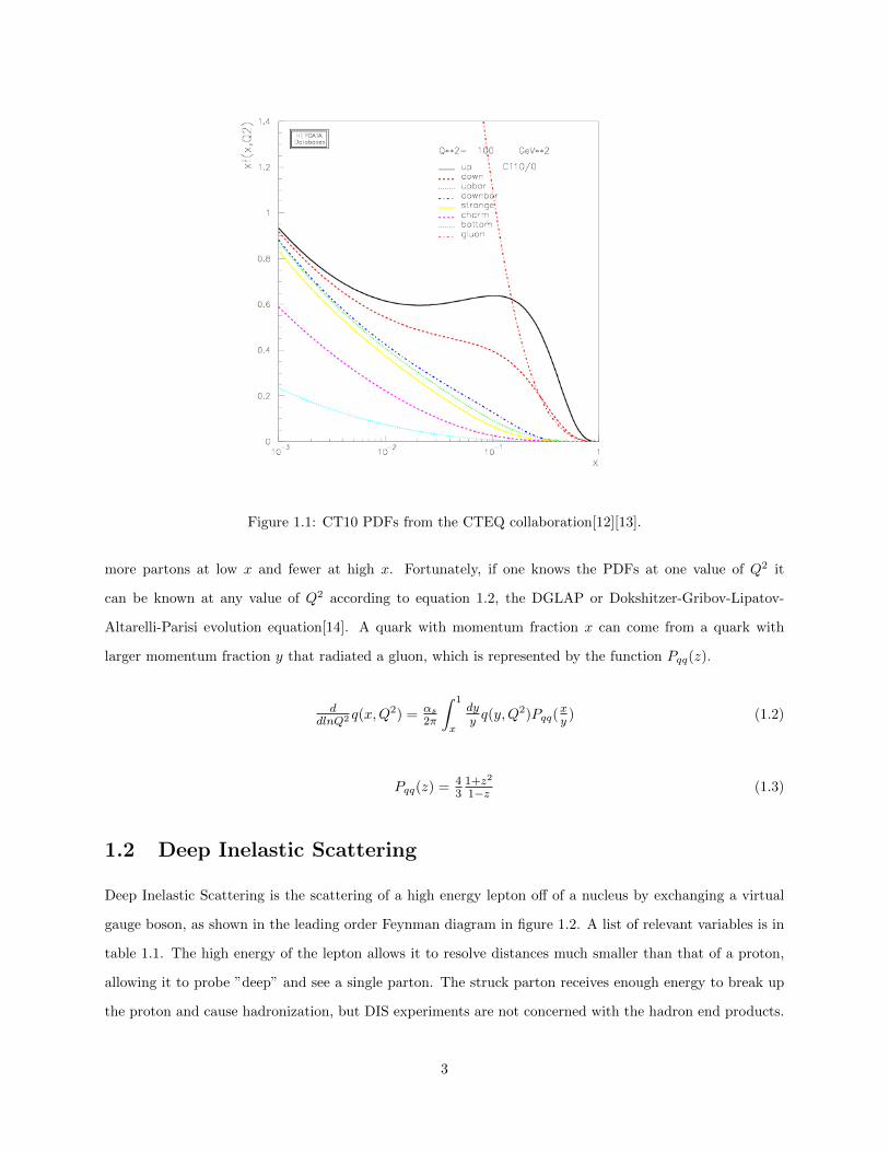
Figure 1.1: CT10 PDFs from the CTEQ collaboration[12][13].

more partons at low x and fewer at high x. Fortunately, if one knows the PDFs at one value of Q2 it

can be known at any value of Q2 according to equation 1.2, the DGLAP or Dokshitzer-Gribov-Lipatov-

Altarelli-Parisi evolution equation[14]. A quark with momentum fraction x can come from a quark with

larger momentum fraction y that radiated a gluon, which is represented by the function Pqq(z).

ddlnQ2 q(x,Q

2) = αs

2π

∫ 1

x

dyyq(y,Q2)Pqq(

xy

) (1.2)

Pqq(z) = 43

1+z2

1−z (1.3)

1.2 Deep Inelastic Scattering

Deep Inelastic Scattering is the scattering of a high energy lepton off of a nucleus by exchanging a virtual

gauge boson, as shown in the leading order Feynman diagram in figure 1.2. A list of relevant variables is in

table 1.1. The high energy of the lepton allows it to resolve distances much smaller than that of a proton,

allowing it to probe ”deep” and see a single parton. The struck parton receives enough energy to break up

the proton and cause hadronization, but DIS experiments are not concerned with the hadron end products.

3

DIS experiments calculate q from the change in lepton momentum, which is in turn used to calculate x

using equation 1.4. At high enough Q2 it is possible to approximate the DIS cross section as equation 1.5,

assuming the gauge boson exchanged is a virtual photon. By measuring the cross section as a function

of x, it is possible to get a measure of the parton distribution functions. While DIS has been very useful

for exploring PDFs, the basic electron/muon emits a virtual photon DIS is not sensitive to the difference

between a quark and its antiquark, as seen in equations 1.5, 1.6, and 1.7. Semi-includisve DIS (SIDIS),

which measures some of the hadronization end products, can give us some insight into the antiquark PDFs.

Neutrino DIS can explore such things with the emission of W bosons instead of photons but the details of

other forms of DIS are outside the scope of this paper.

Figure 1.2: Feynman diagram for deep inelastic scattering. Time flows from left to right. The particleexchanged does not have to be a photon, it can be any electroweak gauge boson.

x =Q2

2P ·q (1.4)

dσdE′dΩ

= α2

4E2sin4(θ/2)(F2(x)v

cos2(θ/2) +2F1(x)M

sin2(θ/2)) (1.5)

4

Variable Description

ki, kf Initial and final lepton 4-momentumq Gauge Boson 4-momentumP Proton 4-momentumE Initial energy of the leptonE′ Final energy of the leptonv E - E’, energy of the gauge bosonM Proton massθ Scattering angle of the leptonQ2 −q2, energy scale of the processx Bjorken scaling variableα Fine structure constantqi(x) PDF of quark flavor iei Electric charge of quark flavor i, as a fraction of eΣi Means sum over all quark flavors

Table 1.1: A list of relevant variables in DIS.

F1(x) = 12Σie

2i (qi(x) + qi(x)) (1.6)

F2(x) = Σie2ix(qi(x) + qi(x)) (1.7)

1.3 Drell-Yan Process

The Drell-Yan process[15] is where a quark antiquark pair annihilate into a virtual photon (or Z-boson) that

then decays into a lepton antilepton pair, as shown in figure 1.3. A list of the relevant variables for the

Drell-Yan process is shown in table 1.2. The leading order Drell-Yan cross section can be quickly derived

from the simple e+e− −→ µ+µ− leading order cross section, shown in equation 1.8[5].

σ(e+e− −→ µ+µ−) = 4πα2

3s(1.8)

The first change that is necessary is that the mass of the virtual photon of the Drell-Yan process is not

the same as s of the proton nucleon collision, so s becomes M2. Second, the structure of the proton has to

be taken into account, so the total cross section is a double integral over all the partons in the beam proton

and all the partons in the target nucleon. One must take into account that a quark can only annihilate with

a matching flavor of anti-quark, and that the likelihood of this annihilation is proportional to e2i . Third, a

factor of 1/3 must be added as the annihilation has to match colorwise, i.e. red can only annihilate with

antired. These changes result in equations 1.9 and 1.10.

5

σDY = 4πα2

9

∫ 1

0

∫ 1

0

Σie2iM2 (qi(xB)qi(xT ) + qi(xB)qi(xT ))dxBdxT (1.9)

dσDY

dxBdxT= 4πα2

9M2 Σie2i (qi(xB)qi(xT ) + qi(xB)qi(xT )) (1.10)

Looking at the equation for the Drell-Yan cross section we can see that unlike basic DIS the term for

a quark from the target is not symmetric with the term for an antiquark from the target. If one uses an

antiproton beam on a proton target the cross section changes to equation 1.11, giving yet another avenue of

attack for distinguishing between quark and antiquark PDFs.

dσDY

dxBdxT= 4πα2

9M2 Σie2i (qi(xB)qi(xT ) + qi(xB)qi(xT )) (1.11)

If one wants to simulate Drell-Yan reactions with Monte Carlo, the angular differential cross section (or

at least the angular dependence of 1 + cos2(θ)) in equation 1.12 is also needed.

σDY

dΩ|cm = α2

4(1 + cos2(θ))

∫ 1

0

∫ 1

0

Σie2iM2 (qi(xB)qi(xT ) + qi(xB)qi(xT ))dxBdxT (1.12)

Figure 1.3: Feynman diagram for the Drell-Yan process. Time flows from left to right. The particle exchangedcould also be a Z-boson, but at SeaQuest our energies are too low.

Several of the measured variables in Drell-Yan are related to one another. Out of the four variables, M ,

xF , xB , and xT , if you know two of them the other two can be calculated via equations 1.13 through 1.16.

However, these are only approximate, and a more in depth calculation of xB and xT from experimentally

measured variables is found in the analysis chapter. Still, using these approximations, it is possible to

transform equation 1.10 into equation 1.17 by using a Jacobian to do a change of variables.

6

Variable Description

k Initial 4-momentum of the quark from the beam protonj Initial 4-momentum of the quark from the target nucleonq Virtual photon 4-momentums Invariant mass squared of the proton nucleon system, c.m. frameP1 Beam proton 4-momentumP2 Target nucleon 4-momentumM Invariant mass of the µ+ µ− pairQ2 −q2, energy scale of the processxB Bjorken scaling variable, beam parton, sometimes called x1

xT Bjorken scaling variable, target parton, sometimes called x2

xB Feynman x, longitudinal momentum of the virtual photon, di-vided by the maximum it could have

y Rapidity, 12ln(

E+p‖E−p‖

)

τ M2/sθ Angle of µ− with respect to the z-axis in the Collins Soper frameφ Azimuthal angle of µ− measured with respect to qT in the Collins

Soper frameα Fine structure constantqi(x) PDF of quark flavor iei Electric charge of quark flavor i, as a fraction of eΣi Means sum over all quark flavors

Table 1.2: A list of relevant variables in the Drell-Yan process used in the SeaQuest experiment.

M ≈√sxBxT (1.13)

xF ≈ xB − xT (1.14)

xB ≈xF +√x2F +4M2/s

2(1.15)

xT ≈−xF +

√x2F +4M2/s

2(1.16)

dσDY

dMdxF= 8πα2

9M3xBxTxB+xT

Σie2i (qi(xB)qi(xT ) + qi(xB)qi(xT )) (1.17)

After Drell and Yan published their paper, experimental data on the differential cross section of the Drell

Yan process showed a few surprising results[16]. First, there were dileptons with transverse momentum

much higher than the expected 300 to 500 MeV[17][18]. Second, while the shape of the differential cross

section was close to what was expected, the total cross section was off by approximately a factor of 2. This

7

factor is called the K factor, and the next to leading order (NLO) cross section terms are responsible for this

K factor[19]. The significant contribution of NLO terms are also responsible for the higher than expected

observed pT . A plot of pT in Drell-Yan experiments is shown in figure 1.4.

Figure 1.4: A graph of the average pT versus√s[16].

When the Drell-Yan process has high pT , it is no longer reliable to calculate θ in equation 1.12 as the

angle between the beam axis and ~µ−. Because of this, Collins and Soper came up with the Collins Soper

frame[20]. This frame is the center of mass frame of the dilepton pair, with the z axis chosen to bifurcate the

angle between ~P1 and −~P2. θ is measured as the angle between this axis and ~µ−. Defining a vector qT as

the unit vector in the (~P1, ~P2) plane orthogonal to the z-axis, the azimuthal angle φ for µ− is defined with

respect to qT . qT is sometimes the definition of the x-axis but Collins and Soper preferred not to define an

x or y-axis. A more intuitive way to calculate φ is as the angle between the dilepton plane and the dihadron

plane. A visual diagram of this frame is displayed in figure 1.5.

1.4 Gottfried Sum Rule

The naive expectation among most physicists at the time was that u(x) = d(x). One expression of this

expectation was the Gottfried sum rule[22], which was that the Gottfried Sum, SG, is equal to 1/3. The

Gottfried sum is shown in equation 1.18 and is a function of the difference between proton and neutron

8

Figure 1.5: A diagram of the Collins Soper plane[21].

structure functions.

SG =

∫ 1

0

(F p2 − Fn2 )dxx

(1.18)

Subbing in from equation 1.7, we get equation 1.19.

SG =

∫ 1

0

Σie2i (q

pi + qpi − q

ni − qni )dx (1.19)

The strange and heavier quarks are expected to have the same distributions for protons and neutrons,

so those contributions cancel out. Isospin symmetry gives us un(x) = dp(x), dn(x) = up(x), un(x) = dp(x),

and dn(x) = up(x). This leads to equation 1.20.

SG =

∫ 1

0

13(u(x) + u(x)− d(x)− d(x))dx (1.20)

Adding a 2/3(u(x)− u(x)) and a similar term for d(x) gets us equation 1.21.

SG = 13

∫ 1

0

(u(x)− u(x))dx− 13

∫ 1

0

(d(x)− d(x))dx+ 23

∫ 1

0

(u(x)− d(x))dx (1.21)

∫ 1

0(u(x)− u(x))dx = 2 and

∫ 1

0(d(x)− d(x))dx = 1 as the proton has valence content of two u quarks and

one d quark, which gives us equation 1.22.

SG = 13

+ 23

∫ 1

0

(u(x)− d(x))dx (1.22)

If d(x) = u(x), then SG = 1/3.

9

1.5 Sea Flavor Asymmetry in Past Experiments

The purpose of the SeaQuest experiment is to study the asymmetry in the parton sea, d(x) 6= u(x). The

study of this asymmetry started with the New Muon Collaboration (NMC) experiments who first discovered

this and continues today with SeaQuest.

1.5.1 New Muon Collaboration

The NMC were not the first experiment to measure the Gottfried Sum, but the others had large uncertainties

and the NMC were the first to find out that SG 6= 13 [23]. They found a value of SG = 0.24 ± 0.016,

unambiguously below the 13 of the expected value. They used two muon beams of energies 90 and 280 GeV

to do DIS on hydrogen and deuterium targets. The definition of F d2 in the NMC papers is sometimes F p2 +Fn2

and sometimes (F p2 + Fn2 )/2, I will consistently use the former definition. First, the NMC calculated the

ratioσdσp

from the ratio of events on their hydrogen and deuterium targets[24]. Then they calculated the

ratio of the structure functions via equations 1.23 and 1.24

F d2

F p2

=σdσp

(1.23)

Fn2

F p2

=F d2

F p2− 1 (1.24)

After the ratioFn

2

Fp2

was calculated, the NMC then calculated F d2 from a fit to data from several DIS

experiments. With these values, they then calculated F p2 − Fn2 via equation 1.25.

F p2 − Fn2 = F d2

1−Fn2

F p2

1+Fn2

F p2

(1.25)

This calculation was done separately for many different bins in the x range 0.004 to 0.8. The NMC

plotted this data on a graph in figure 1.6 and extrapolated the integral of∫ 1

x(F p2 − Fn2 )dxx data to x = 0 to

calculate SG.

1.5.2 NA51

NA51 was designed to test between two hypotheses to explain the SG result from NMC[25]. The first

hypothesis was that the contents of the proton at x < 0.004 make a large contribution to SG and therefore

the extrapolation of NMC from x = 0.004 to 0 was not valid. The second hypothesis was that the quark

10

Figure 1.6: Data from NMC. The black points use the scale to the right and are F p2 − Fn2 for that bin in x.The white points use the scale to the left and are the integral of F p2 − Fn2 from that value of x to 1. Thewhite points are extrapolated to reach a value of SG, which is significantly below the predicted value of 1/3(Labelled with QPM).

sea was asymmetric, d(x) 6= u(x). NA51 used a 450 GeV proton beam on hydrogen and deuterium targets

and compared their Drell-Yan cross sections. They assumed shadowing, which is an effect that modifies the

PDFs when the nucleons are inside of a nucleus, was negligible and that σpd = σpp + σpn. NA51 defined a

quantity ADY in equation 1.26 and measured it as in equation 1.27.

ADY = σpp−σpn

σpp+σpn (1.26)

ADY = 2σppσpd− 1 (1.27)

In the kinematics of NA51, y ≈ 0 and x1 ≈ x2. NA51 treated the contributions of interactions between

two sea partons as insignificant, which led to the proton and neutron cross sections being proportional to

equations 1.28 and 1.29.

σpp ∝ 8uv(x)u(x) + 2dv(x)d(x) (1.28)

σpp ∝ 5uv(x)d(x) + 5dv(x)u(x) (1.29)

All of the constants in front of the parton distributions cancel out and when we sub equations 1.28 and

11

1.29 into equation 1.26 we end up with equation 1.30.

ADY =(4uv−dv)(u−d)+(uv−dv)(4u−d)

(4uv+dv)(u+d)+(uv+dv)(4u+d)(1.30)

Defining the ratio of valence quarks as λv = uv/dv and the ratio of sea quarks as λs = u/d we end up

with equation 1.31.

ADY =(4λv−1)(λs−1)+(λv−1)(4λs−1(4λv+1)(λs+1)+(λv+1)(4λs+1)

(1.31)

This equation can be solved for λs, shown in equation 1.32

λs =2−5λv−2ADY −5ADY λv5−8λv+5ADY +8ADY λv

(1.32)

NA51 calculated one value for λs at an average value for x or 0.18. They used a value of λv(0.18) =

2.2 taken from an average of several PDFs and measured ADY from their experiment. After calculating

corrections for the sea-sea terms they neglected in their approximation, in 1994 they published results

showing a value of λs = 0.51±0.04(sta)±0.05(sys), which translates into d/u = 1.96±0.15(sta)±0.19(sys).

1.5.3 E866/NuSea

The E866 experiment was a fixed target experiment at Fermilab using an 800 GeV proton beam on hydrogen

and deuterium targets[26]. It used a spectrometer that favored events where xB > xT . It is similar to our

own experiment, sharing some wire chambers, collaboration members, Monte Carlo code, and a similar

design. E866 measured the Drell-Yan cross section ratio σpd/σpp and used that to estimate d/u. In the

kinematic region xB > xT it is much more likely that the antiquark comes from the target than the beam

due to the large ratio of quarks to antiquarks at higher x. The ratio of the Drell-Yan differential cross section

for proton-proton and proton-deuterium collisions is in equation 1.33 if one neglects strange and higher mass

quarks and also drops the terms where the antiquark comes from the beam.

σpdσpp

= 1 +4u(xB)d(xT )+d(xB)u(xT )

4u(xB)u(xT )+d(xB)d(xT )(1.33)

By recognizing that 4u is greater than d by a factor of 8 and making an approximation where the d terms

in the ratio are omitted, we receive equation 1.34.

σpdσpp

= 1 +d(xT )u(xT )

(1.34)

12

This much of an approximation is clearly unfit for calculating real physics results but it shows the

sensitivity of the measurement of the cross section ratio to d/u in forward spectrometer Drell-Yan experiments

such as E866 and SeaQuest. NuSea’s actual calculation used an iterative process where a prediction for the

cross section ratio σpd/σpp was calculated based on a hypothetical value for d/u. This predicted ratio was

compared to the measured ratio and d/u was adjusted accordingly for the next iteration. The quark PDFs

and d(x)+u(x) values were taken from the CTEQ4M PDFs. The iteration converged on a value for d(x)/u(x)

when the predicted and measured cross section ratios matched. In 1998 E866 published results showing a

dependence of d(x)/u(x) on x. A plot of the cross section ratio results are shown in figure 1.7 and the sea

flavor asymmetry results are shown in figure 1.8 from the improved measurement results from 2001[27]. An

interesting feature of the improved results is the high x point where d < u with a certainty greater than 1 σ.

Figure 1.7: The cross section ratio σpd/2σpp results binned in x for E866. Predictions from various PDFsare also shown.

1.6 Motivation

The Drell-Yan process can be used to study the PDFs in a way complementary to DIS experiments. Drell-

Yan has sensitivity to sea quarks and can be used to research the antiquark PDFs, especially with a forward

spectrometer. The SeaQuest experiment was designed to pick up where E866 left off and research the

13

Figure 1.8: d/u binned as a function of x, from E866. Predictions from various PDFs are also shown.There is a significant difference at high x for PDF sets published before the E866 results in 1998 and thosepublished after the E866 results. The drop below d/u = 1 at higher x was completely unexpected.

14

d(x)/u(x) distribution at even higher x[28][29]. The Drell-Yan cross section drops off quickly with higher

mass, as shown in figure 1.9 and equation 1.10, and high mass dimuons are high x dimuons. Because of this,

some way to improve the statistics of the measurement was needed in order to design an experiment that

measured higher x antiquark PDFs than E866. Rewriting equation 1.10 to put the M2 in terms of s, we can

see that the Drell-Yan cross section is inversely proportional to s.

Figure 1.9: The dimuon mass spectrum from E866. Notice the J/Ψ and Ψ′ peaks between 3 and 4 GeV. Italso drops off quickly with mass[30].

dσDYdxBdxT

= 4πα2

9sxBxTΣie

2i (qi(xB)qi(xT ) + qi(xB)qi(xT )) (1.35)

Calculating s shows us it is very close to being proportional to the beam energy.

s = mt ∗ EBeam +m2t +m2

b (1.36)

15

SeaQuest uses a beam energy of 120 GeV, which gives about an improvement of 6.7 times more cross

section than the 800 GeV beam of E866. Another improvement is that SeaQuest can support higher lumi-

nosity. As radiation dosage scales with beam energy SeaQuest can have a higher luminosity without going

over radiation safety limits. Background also scales with luminosity, and the main background of E866 was

muon singles from J/Ψ decay. As can be seen in figure 1.10, the J/Ψ production cross section rises quickly

with√s, so SeaQuest can have a higher luminosity without running into background troubles.

√s for a

proton-proton reaction is about 38.76 GeV for E866 and 15.06 GeV for SeaQuest. The proposal for SeaQuest

estimated a factor of 50 increase in statistics compared to E866, with estimated statistical uncertainties by

the end of the experiment estimated in figure 1.11. This high x region is of much interest, as E866 suggests

d < u in that region and no known model predicts this. The results of E866 were interesting but of not

enough statistical significance to be compelling, SeaQuest’s flagship measurement of d/u aims to answer the

question, ”Does d/u really fall below 1?”

Figure 1.10: The J/Ψ cross section as a function of√s. It grows quickly with higher energies[31].

1.7 Models

One early hypothesis was that Pauli blocking was the cause of the sea flavor asymmetry, as the two valence

u quarks blocked u more than the valence d quark blocked d[32]. However, it has been shown that Pauli

16

Figure 1.11: Estimated statistical uncertainties for SeaQuest, compared to E866[29]. While we have fallenshort of this goal, we have still improved upon the E866 measurement from about x = 0.15 to 0.35 androughly measured the asymmetry at x up to 0.58.

17

blocking does not contribute to the excess of d[33]. Since then, many models have been proposed to explain

the d/u asymmetry[34]. As stated earlier, none of them predict d < u at any x. Figures for predictions

of the meson cloud model, chiral quark model, chiral quark soliton model, and the statistical model are in

figures 1.12, 1.13, 1.14, and 1.15. An explanation of each model is outside the scope of this paper.

Figure 1.12: Comparison of two similar meson cloud models to E866 data. The dotted line parametrises thepion as having an effective mass of 400 MeV inside the proton. Both approach d = u at high x[35].

18

Figure 1.13: E866 data and the NA51 data point plotted with two variants of the Chiral Quark model (redand blue curves). The authors note that they could not get the ratio below 1 in their models[36].

Figure 1.14: A comparison of E866 and NA51 data with a Chiral Quark Soliton model (solid line) andseveral PDF sets[37]. This uses the early E866 data without a statistically significant d < u.

19

Figure 1.15: A statistical model compared to E866 data. The solid line is the prediction from the statisticalmodel[38]. In this model d/u keeps increasing.

20

Chapter 2

Experimental Setup

This chapter is a basic introduction to the spectrometer at SeaQuest. It covers how the measurements used

in this analysis were made. It also examines the origins of many of the challenges of this analysis, particularly

those related to beam quality and target purity.

SeaQuest is a fixed target experiment that takes place at Fermilab and uses the 120 GeV proton beam

from the main injector. A diagram of our spectrometer can be found in figure 2.1. The beam passes by or

through detectors placed to monitor the strength of the beam. It then strikes our choice of one of seven

targets, producing the dimuons we are interested in analysing and a large number of background particles.

Behind the targets is FMag (Fe Magnet), a thick iron core magnet that focuses dimuons inwards and also

acts as a beam dump. Located behind FMag are many detectors for tracking the muons, these include

several planes of hodoscopes, drift chambers, and propulsion tubes. These detectors are sorted into four

tracking stations. Station 1 is just behind FMag. Between stations 1 and 2 is KMag (kTev Magnet), an

air core magnet previously used by kTev that bends the incoming muons so that their momentum can be

calculated. Station 2 is behind KMag, followed by a gap in the spectrometer and then station 3. Between

stations 3 and 4 is about a meter of iron that is used to block any hadronic matter that is left. Station 4

is mainly used for muon identification. Hodoscopes in each station are fed into a trigger matrix where the

right combination of input signals will cause the DAQ to read out the data from that event. The prop tubes

and drift chambers in each station are used for track reconstruction.

The beam travels in the positive z direction. The positive y direction is straight upwards and the positive

x direction is defined by requiring a right handed coordinate system. The origin of the coordinate system is

the location where the beam strikes the front of FMag.

21

Figure 2.1: A figure of the SeaQuest spectrometer.

2.1 Timeline

Changes have been made to our setup throughout our experiment. Detectors have been moved out and

back in for repairs, requiring new surveys. The trigger matrix has been updated. The magnet polarity has

been flipped. The deuterium has been replaced with new bottles that have different contamination levels.

All of these things affect the analysis of the data. Table 2.1 contains the dates of each roadset (roadsets

will be explained in the Trigger section) and a few other significant events relevant to the analysis. Runs

in this experiment are major data taking divisions, which mark significant events such as moving from

commissioning to viable data taking or the installation of a new detector. The first viable data starts in run

2 and of this writing the experiment has finished run 5.

22

Run Event Date

2 Roadset 57 06/25/2014 to 08/20/2014Roadset 59 08/20/2014 to 09/03/2014

N/A D3p and D3m moved 10/03/2014

3 Roadset 62 11/08/2014 to 01/14/2015Deuterium Change 11/13/2014Deuterium Change 12/02/2014Magnet Polarity flipped 01/14/2015Roadset 67 01/25/2015 to 06/19/2015Deuterium Change 04/24/2014D1 and H1 moved 05/13/2015Roadset 70 06/19/2015 to 07/03/2015

4 Constant adjustments 11/13/2015 to 03/06/2016

5 Roadset 78 03/06/2016 to 07/29/2016

Table 2.1: A table of important dates for this data analysis.

2.2 Beam

The 120 GeV beam energy that SeaQuest uses is a low beam energy compared to other Drell-Yan experiments,

and this gives three main advantages[29][28]. First, the Drell-Yan cross section scales with 1/E, where E is

the energy of the beam. This increases the cross section by about a factor of seven compared to the previous

experiment, E866. Secondly, radiation dose roughly scales with beam power, and a lower beam energy means

one can have a higher luminosity but still have the same beam power and radiation. E866 received 2e12

protons during their 20 second spill, once per minute. E906 receives an average of 6e12 protons each five

second spill, once per minute. The third advantage is background reduction. J/Ψ production was a large

source of muons in the detectors in E866 but J/Psi production is lower by about a factor of eight, according

to the fit in Measurement of J/Ψ and Ψ’ production in 800 Gev/c proton-gold collisions[31]. Most other

backgrounds scale with s which is roughly proportional to the beam energy in a fixed target experiment.

The beam has a frequency of 53.1 MHz; SeaQuest receives a group of protons about every 18.8 ns. These

groups of protons are no more than 2 ns long and are called buckets. Each bucket is part of a booster

batch that is about 83 buckets long. There is a gap of about three buckets between each booster batch.

A combination of six booster batches and a long gap of about 80 buckets makes up a single turn, which is

exactly 588 buckets. There are 369,000 turns in a single five second spill. Every minute SeaQuest receives

a five second spill followed by 55 seconds of no beam.

The beam provided to SeaQuest has unfortunate issues with non-uniformity. The beam contains a large

number of ”super buckets” that contain many more protons than the average bucket, as can be seen in

figure 2.2, these events are nicknamed ”splat events”. These cause so many tracks that often more of the

23

detector elements have a hit than don’t have a hit, as can be seen in figure 2.3. A clean event is provided

for comparison in figure 2.4. A super bucket that lights up almost the entire detector is almost guaranteed

to satisfy the trigger, but the event is so messy that it is extremely unlikely that any dimuon in the data

can be reconstructed. When the trigger requirements are met the DAQ reads out the data which prevents

any more data from being taken until the DAQ is finished. This dead time is proportional to the number

of hits in the event, which makes these super buckets a particularly bad type of garbage event as they can

cause several hundred µs of dead time.

Figure 2.2: A plot of protons in each bucket. The booster batch and turn structure is visible. A typicalreconstructed event has 25,000 protons and our intensity cut (data quality cut, not inhibit threshold) is at60,000 protons. Super bucket spikes (those crossing the red line) are visible about once a turn. A singlesuper bucket causes dead time for dozens of turns if it is not inhibited.

Figure 2.3: A diagram of a splat event, generated by the SeaView program. Most of the detector elementshave fired.

A measure of the beam quality is the duty factor. Duty factor is usually given as a percent, and a duty

factor of 100% would have a perfectly uniform distribution of protons between the buckets. The formula

is in equation 2.1. When the experiment first began the duty factor was about 29%. This was much lower

than expected, as the previous experiment E866 enjoyed a duty factor between 70% and 80%. In the middle

24

Figure 2.4: A diagram of a clean event, generated by the SeaView program. It is much more clear than thesplat event.

of December 2014, the duty factor improved drastically to an average of about 43%. This event is known as

the Christmas miracle.

duty factor =(∑n

i I)2

n∑n

i I2 (2.1)

When we first started taking data, the recorded events were dominated by un-analysable super bucket

events. The eventual solution was to install a Cerenkov counter in the beam line that outputs an analog

signal proportional to the number of protons passing through it. The Cerenkov counter output was connected

to a charge integrator and encoder(QIE) circuit board, which converted the total analog signal over the

duration of a bucket into a digital signal. The QIE is synchronized with the Main Injector RF clock so that

the integration intervals align with the buckets. If the QIE output is higher than a programmed inhibit

threshold then the trigger can not fire for that bucket or for eight buckets before or after the offending

bucket. Currently, this trigger inhibit blocks about 40% of the incoming protons. The trigger inhibit is also

sometimes called the QIE inhibit or the beam monitor veto.

The QIE provides a lot of useful information as well as the trigger inhibit. When an event is read out, the

QIE values for the triggering bucket and 16 buckets before and after the trigger are recorded. This is crucial

for understanding the rate dependence of SeaQuest. It is also useful for normalizing data by the number of

protons on target. The QIE records the total QIE value for the entire spill, the total QIE value while the

trigger was inhibited, and the total QIE value while the trigger was not inhibited but we had dead time due

to DAQ read out. These values are QIEsum, inhibit block sum, and trigger sum no inhibit respectively and

are in the BeamDAQ table.

To properly use the QIE numbers it is important to understand a couple of things. The QIE has a

25

pedestal, which is a non zero value that it reads out when there is no incoming beam. That number must

be subtracted from any QIE values that are used. Also, the number that is read out is not the number

of protons. A measure of the total number of protons for that spill, such as S:G2SEM in the Beam table

or NM3ION in the BeamDAQ table, needs to be used to convert QIE values to protons. The conversion

factor for QIE value to protons is QIESum/S:G2SEM. This number is not constant. The conversion factor

gradually drifts over time as the mirror degrades over the course of several weeks. It also jumps suddenly if

the mirror or the neutral density filters are replaced. This means this conversion factor should be calculated

separately for every spill. Using all this information equation 2.2 can be used to calculate the number of

live protons in the spill, which is the number of protons in the spill where the trigger was active and it was

possible to take data and is the relevant measure of intensity.

live protons = S : G2SEMQIESum−inhibit block sum−trigger sum no inhibit

QIESum(2.2)

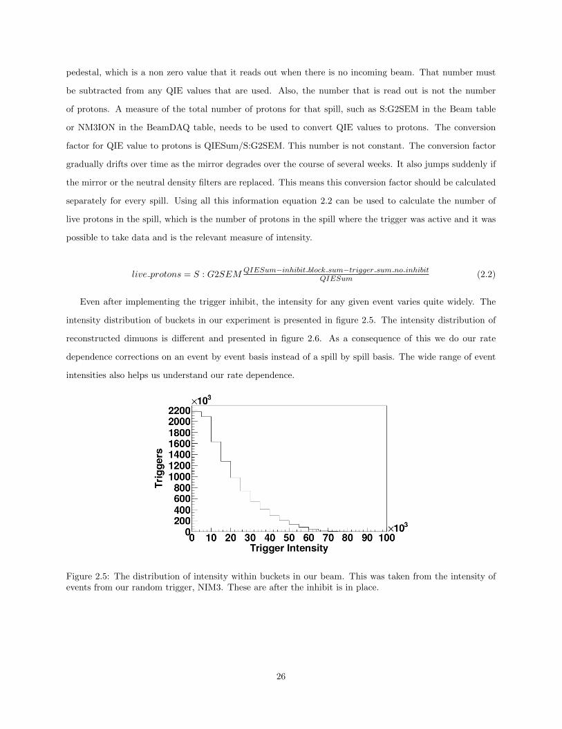
Even after implementing the trigger inhibit, the intensity for any given event varies quite widely. The

intensity distribution of buckets in our experiment is presented in figure 2.5. The intensity distribution of

reconstructed dimuons is different and presented in figure 2.6. As a consequence of this we do our rate

dependence corrections on an event by event basis instead of a spill by spill basis. The wide range of event

intensities also helps us understand our rate dependence.

Figure 2.5: The distribution of intensity within buckets in our beam. This was taken from the intensity ofevents from our random trigger, NIM3. These are after the inhibit is in place.

26

Figure 2.6: The distribution of intensity of triggering buckets in reconstructed dimuons.

2.3 Targets

SeaQuest uses seven different targets which are placed on a target rotation table, a diagram of which is in

figure 2.7. The two liquid targets are flasks filled with liquid hydrogen (LH2) and liquid deuterium (LD2).

There is a third flask of the same dimensions that contains vacuum which is for correcting for background

that appears to come from the target. There are three solid targets made out of iron, carbon, and tungsten.

There is a fourth solid target slot on the target table that contains nothing and is called the none target,

this is also for background subtraction. Each solid target is actually made out of three separate discs that

are spaced apart to attempt to cancel out any z position dependence in acceptance when comparing to the

liquid targets. The center of the targets are at the position of 129.5 cm in front of the face of FMag. The

liquid targets and the empty flask have a length of 50.8 cm. One target is in the path of the beam at a

time, and the targets are changed in the 55 second gap between spills. A typical target rotation lasts about

23 spills, and then goes in reverse order for another 23 spills. This constant rotation avoids any systematic

differences between the targets that could be caused by any feature of the spectrometer slowly changing over

time. When we first started taking data there were 10 spills on the LH2 target and five spills on the LD2

target for every spill on the empty flask. Currently it is 10 spills on LH2 and five spills on LD2 for every two

spills on the empty flask. Each target has an integer assigned to it that is used to identify it in our data.

These integers can be found in table 2.2.

For a significant portion of our data taking our deuterium target was filled with impure deuterium. This

was expected, but the puzzling aspect of this contamination is that it is significantly different between all

four deuterium samples that were analysed. The four samples come from different bottles of deuterium in

our experiment which were all filled many years ago at the same time from the same tube trailer which was

27

Figure 2.7: A diagram of the target table.

Target Material Target Number

Liquid Hydrogen 1Empty Flask 2Liquid Deuterium 3No Target 4Iron 5Carbon 6Tungsten 7

Table 2.2: List of target identifiers

28

filled from a Fermilab bubble chamber. Some of the samples were filled from the bottles and some of the

samples were filled from the target flask. Each sample has been analysed twice and the different analyses

on the same samples are very consistent, with differences on the order of less than 0.1%. This has led

to people asking if we have introduced major contamination during the sampling process and if all three

bottles really do have the same composition. These theories have additional weight because some of the

samples have significant N2 and O2 components, suggesting contamination by air. Additionally, hydrogen

can diffuse into metal surfaces, so often containers are baked under vacuum in order to remove the hydrogen

contamination. Word of mouth from Fermilab is that the bottles that hold our deuterium were probably

not baked out before being filled with deuterium, although there is no documentation about the procedure

used to fill them. We know that the target flasks and sample bottles were not baked out before being filled

with deuterium, and that the deuterium target flask has been tested with hydrogen several times to avoid

wasting the more expensive deuterium.

The samples taken have small amounts of helium and heavier nuclei. We have decided to work under

the assumption that the heavier nuclear molecules are caught in the cold trap in the cryogenics system and

do not make it into the target. We also assume that the helium exists in a gaseous state at the top of the

target and does not interact with the proton beam. We then use the ratios of H2, HD, and D2 to calculate

the contamination while assuming the H2, HD, and D2 adds up to 100%. We treat all the sample analyses

as correct when deciding where to place the cross section ratio points, but use the minimum and maximum

contaminations between all the samples as systematic uncertainties. SeaQuest continues to look into this

and hopes to reduce the uncertainty from this value. Partway through roadset 67, we switched to commercial

deuterium. This commercial deuterium is pure to a high level of precision. Our 1H gas has always been

very pure as well.

The amount of contamination and its uncertainty by run number is found in table 2.3. There are a

few different run ranges with different contamination levels, and transitions between these run ranges often

happen in the middle of a roadset. For roadsets or combinations of roadsets where the contamination changes

partway through, I average the contamination over all deuterium dimuons. The results of this averaging are

in table 2.4.

To calculate a cross section requires some knowledge of the target properties. The lengths of the targets

are 20 inches ± 2.5 mm. The nuclear interaction lengths (NIL) in g/cm2 and atomic masses were taken from

the particle data group[39]. The target densities at our pressure and temperature were taken from National

Institute of Standards and Technology[40]. The values for the deuterium targets need to be corrected for

the 1H contamination. Using A as atomic mass, λ as the nuclear interaction length (in g/cm2), ρ as the

29

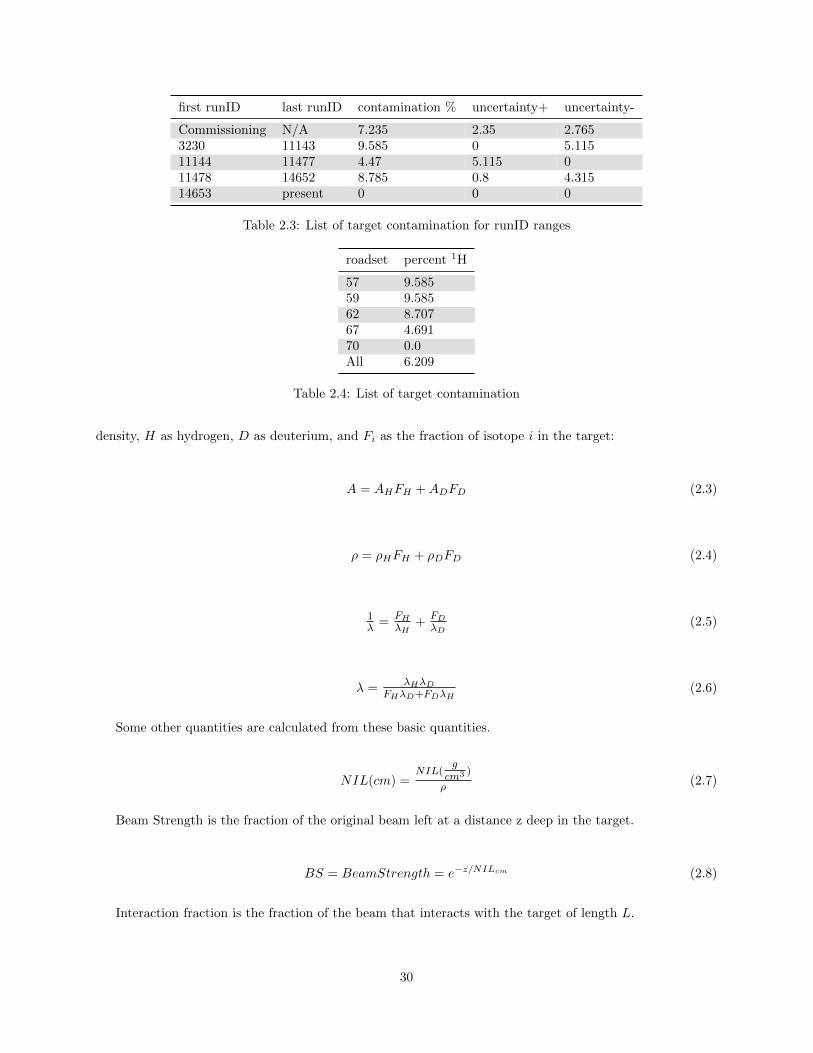
first runID last runID contamination % uncertainty+ uncertainty-

Commissioning N/A 7.235 2.35 2.7653230 11143 9.585 0 5.11511144 11477 4.47 5.115 011478 14652 8.785 0.8 4.31514653 present 0 0 0

Table 2.3: List of target contamination for runID ranges

roadset percent 1H

57 9.58559 9.58562 8.70767 4.69170 0.0All 6.209

Table 2.4: List of target contamination

density, H as hydrogen, D as deuterium, and Fi as the fraction of isotope i in the target:

A = AHFH +ADFD (2.3)

ρ = ρHFH + ρDFD (2.4)

1λ

=FH

λH+

FD

λD(2.5)

λ =λHλD

FHλD+FDλH(2.6)

Some other quantities are calculated from these basic quantities.

NIL(cm) =NIL(

gcm3 )

ρ(2.7)

Beam Strength is the fraction of the original beam left at a distance z deep in the target.

BS = BeamStrength = e−z/NILcm (2.8)

Interaction fraction is the fraction of the beam that interacts with the target of length L.

30

IFrac = InteractionFraction = BSBeforeTarget −BSAfterTarget = 1− e−L/NIL(cm) (2.9)

Target attenuated length is the average target length seen by a proton traversing the target. This is less

than the actual length because some protons don’t make it the full distance.

TargetAttenuatedLength = L′ =

∫ L

0

e−z/NIL(cm)dz (2.10)

L′ = −NIL(cm) ∗ (e−L/NIL(cm) − 1) = NIL(cm) ∗ IFrac (2.11)

Atoms per area is the number area density of atoms in the target, as seen by a proton moving in the z

direction through the target.

AtomsPerArea = ρ ∗ L′/A (2.12)

The target properties are listed in tables 2.5 and 2.6, including for the contaminated deuterium targets.

material length(cm) ρ (g/cm3) NIL (g/cm2) NIL (cm) A (g/mol)

LH2 50.8 ± 0.25 0.0708 52.0 734.5 1.00794LD2 pure 50.8 ± 0.25 0.1634 71.8 439.4 2.01410LD2 57, 59 50.8 ± 0.25 0.1545 69.3 448.3 1.91751LD2 62 50.8 ± 0.25 0.1553 69.5 447.4 1.9262LD2 67 50.8 ± 0.25 0.1591 70.5 443.5 1.9669LD2 All 50.8 ± 0.25 0.1576 70.14 444.9 1.9515

Table 2.5: List of target properties. For the deuterium for a given roadset, note that the contaminationis not necessarily constant, and these properties would not be constant. These are the properties for theaverage contamination.

material IFrac L’(cm) atoms per area (atoms/cm2)

LH2 0.0668 49.08 2.076e24LD2 pure 0.1092 47.97 2.344e24LD2 57, 59 0.1071 48.027 2.331e24LD2 62 0.1073 48.022 2.332e24LD2 67 0.1082 48.00 2.338e24LD2 All 0.1079 48.005 2.335e24

Table 2.6: More target properties. For the deuterium for a given roadset, note that the contamination is notnecessarily constant, and these properties would not be constant. These are the properties for the averagecontamination.

31

2.4 Magnets

The first magnet in the SeaQuest spectrometer, FMag, is located downstream of the target and upstream

of all the detectors. It is an iron core magnet with no air gap between the iron and the coils and is five

meters thick. The field is 2.07 T inside the iron. FMag serves many purposes; it increases our acceptance of

high mass dimuons, it sweeps low momentum particles out of the acceptance, it acts as a beam dump, and

it absorbs hadronic particles produced in the target.

Higher mass dimuons have larger opening angles and thus the muons have more pT . Normally muons

with this much pT would be outside the acceptance of our experiment, but FMag bends the path of the

muons passing through it. Depending on the orientation of the dimuon the muons could be bent outwards

or inwards. Inward bent dimuons are moved into the acceptance of the spectrometer, while the outward

bent ones probably would not have been in the acceptance to begin with. High xT is correlated with high

mass and low statistics, making acceptance at high mass very valuable.

Fmag also helps with background reduction. Any sort of hadron produced in the target is very unlikely

to make it all the way through five meters of iron without being absorbed. While muons aren’t absorbed

through nuclear collisions like hadrons are, muons do lose energy while traversing the magnet and lower

energy particles are bent farther by the magnet, usually bending them all the way out of the acceptance at

low energies. This reduces the amount of low momentum background that makes it into the spectrometer.

Fmag has a hole that is approximately a foot deep and two inches in diameter drilled into the upstream

face of it in the path of the beam. The portion of the beam that does not interact with the target strikes

FMag at the end of the hole, a foot deep into the iron. Having this hole lessens the radiation in the target area

that sometimes has to be accessed by people, both by moving it farther from the targets and by surrounding

the interaction point with more iron.

The five meters of iron that make up FMag come with a significant downside. The amount of multiple

scattering in FMag is significant and it adds a lot of uncertainty to the reconstruction process. According

to the Monte Carlo simulations the average of the absolute value of the pT change from multiple scattering

is 0.44 GeV. As a result all of the kinematic variables have a lot of uncertainty to them. Running the

reconstruction software on simulated J/Ψ tracks from the Monte Carlo ends up reconstructing a peak

with that is smeared to have a half height width of about 300 MeV. Another important variable that has

considerable uncertainty is the z position of the origin of the dimuon. Even with about a meter from the

end of the target to the beginning of FMag there is not a clear separation between the peak from the target

and the peak from the dump when looking at a graph of dimuon reconstructed z position, as seen in figure

2.8. Several cuts had to be applied to clearly separate the target dimuons from the dump dimuons, which is

32

very important if one is interested in the ratio of cross sections between two targets.

Figure 2.8: This graph shows reconstructed GMC dimuons originating from the target, reconstructed GMCdimuons originating from the beam dump, and all reconstructed dimuons from data. The z origin peaksfrom target and beam dump merge and are hard to separate without cutting a lot of data.

The average pT kick in FMag is 3.07 GeV. The peak of the energy loss of a muon travelling through the

magnet is about 7.6 GeV, but the spectrum has a long tail into the higher energy loss region and a short

tail for lower energy loss which puts the mean energy loss at about 8.45 GeV. A graph of the energy loss

distribution is shown in figure 2.9.

The second magnet, KMag, is located between detector stations one and two. It is an air core magnet

with a magnetic field that peaks at 0.31 T in the center. The magnetic field is always parallel with the field

from FMag. The placement between stations one and two causes the track to bend between stations one

and two. Measuring the bend in the track allows us to calculate both the momentum of the track and its

electric charge. The pT kick going through KMag is 0.385 GeV. There is no energy loss since it is an air

core magnet.

The polarities of both magnets were flipped between roadsets 62 and 67. Up to and including roadset 62

the fields pointed in the positive y direction, afterwards they pointed in the negative y direction. This was

done to identify any left / right asymmetries in our spectrometer by comparing data sets before and after

the switch. Another benefit was to reduce the radiation striking most of the electronic equipment, which

was mostly on one side of the spectrometer. With the incoming beam being positive most of the radiation

is also positive so there is an asymmetry in the amount of radiation between the two sides.

The shapes of both of the magnetic fields were calculated and their magnitudes estimated with simulations

33

Figure 2.9: This graph shows the spectrum of energy loss of muons passing through FMag. It was generatedfrom a Geant4 simulation.

done using CST EM Studio. Using the initial magnitudes the reconstruction of data was found to be

inaccurate, with the J/Ψ peak at the wrong mass and the peak for the z origin of dimuons from the target

at the wrong location. The reconstruction of Monte Carlo simulated data placed these peaks in the correct

locations. Monte Carlo simulated data was used to calculate the effects of using inaccurate field strengths

in the reconstruction software. Using the fits shown in 2.10 it was possible to know how much each field

magnitude needed to change in order to accurately reconstruct the data. The multiplier for FMag field

strength was found to be 1.054 and the multiplier for KMag field strength was found to be 0.951. After

these multipliers were added to the tracking software it could accurately reconstruct these peaks in data.

34

Figure 2.10: These graphs show the results of the reconstruction software running on Monte Carlo simu-lated data with a magnetic field strength multiplier. Inaccurate field strengths result in residuals in thereconstruction of the mass and z origin. The mass residual is positively correlated with both the FMag andKMag multipliers, while the z origin residual is positively correlated with the FMag multiplier and negativelycorrelated with the KMag multiplier.

35

2.5 Detectors

The detectors are loosely arranged into four stations, with gaps between the various stations. All of the

stations contain hodoscopes, while only the first three contain drift chambers and only the fourth station

contains proportional tubes (prop tubes). KMag is located between stations 1 and 2 to bend the tracks so

that their momentum can be reconstructed. There are several meters of air between stations 2 and 3 so that

the trajectory after the bend can be measured. There is a meter of iron between stations 3 and 4 that acts

as a hadron absorber so that station 4 can act as a muon identification station, although the majority of

tracks in the first stations should still be leptons.

2.5.1 Hodoscopes

The hodoscopes are detector planes that are made up of several long paddles placed side by side. Each

paddle has a rectangular length made of scintillator, which is a type of material that emits light when struck

by particles passing through. At the end of the rectangle is a shaped piece of scintillator called a light guide,

mostly triangular, that connects to the rectangle at one end and has a narrow cylindrical end at the other

side. This light guide funnels emitted photons from the paddle into a photo-multiplier tube (PMT). The

photo-multiplier tube converts incoming photons to electrons and then amplifies the electric signal so that

it can be read by the DAQ.

The main role of the hodoscopes is to be used as input for the trigger system. The trigger supervisor

looks for preprogrammed combinations of hodoscope paddles, called roads, in order to fire. Hodoscopes are

ideal for triggering because the signal that moves through them is light, so the largest possible drift time is

still much shorter than the difference in time between buckets. With the drift chambers or prop tubes it is

not possible to tell which bucket a signal came from. The width of the hodoscopes and lack of drift distance

information means they are far too coarse to be used in track reconstruction.

There are two types of hodoscopes, x measuring hodoscopes and y measuring hodoscopes. The x mea-

suring hodoscopes have vertically oriented paddles and are spaced horizontally, while the y measuring ho-

doscopes have horizontally oriented paddles and are spaced vertically. In each station there are two sets of

x measuring hodoscopes, one that covers y > 0 and one that covers y < 0. The y measuring hodoscopes are

similarly divided into a left set and right set covering x > 0 and x < 0, respectively. There is one plane of y

measuring hodoscopes in stations 1 and 2, none in station 3, and two planes in station 4. The hodoscopes

in stations 1 and 2 are single ended, while the hodoscopes in stations 3 and 4 are double ended. All of the

hodoscopes have some slight overlap between neighbouring paddles. The names of all the hodoscope stations

begin with ”H”, then the station number, then either ”T”, ”B”, ”L”, ”R”, ”X”, or ”Y” for top, bottom, left,

36

right, x-measuring, or y-measuring. ”X” is the combination of ”T” and ”B” and ”Y” is the combination of

”L” and ”R”. There is an exception for the station 4 y measuring hodoscopes, which instead of using 4 for

the station numbers uses ”4Y1” and ”4Y2”. So the left half of the second station 4 y measuring hodoscopes

would be H4Y1L, and the top half of the station 2 x measuring hodoscopes would be H2T. The dimensions

and z positions of the hodoscopes during run 2 are listed in table 2.7. Some of the hodoscopes had to be

moved out and then back in place between runs 2 and 3. Their positions were surveyed again afterwards.

The positions of the hodoscopes during run 3 are listed in table 2.8 if they changed.

Name # Paddles Paddle Width [cm] Overlap [cm] Width x Height [cm x cm] z-Position [cm]

H1L 20 7.32 0.3175 78.74 x 140.117 654.03H1R 20 7.32 0.3175 78.74 x 140.117 654.03H1B 23 7.32 0.3175 162.008 x 69.85 667.118H1T 23 7.32 0.3175 162.008 x 69.85 667.118H2L 19 13 0.3175 132 x 241.285 1402.86H2R 19 13 0.3175 132 x 241.285 1402.86H2B 16 13 0.3175 203.238 x 152 1421.06H2T 16 13 0.3175 203.238 x 152 1421.06H3T 16 14.5875 0.3175 227.518 x 167.64 1958.51H3B 16 14.5875 0.3175 227.518 x 167.64 1958.51H4Y1L 16 23.4775 0.3175 152.4 x 365.797 2130.27H4Y1R 16 23.4775 0.3175 152.4 x 365.797 2146.45H4Y2L 16 23.4775 0.3175 152.4 x 365.797 2200.44H4Y2R 16 23.4775 0.3175 152.4 x 365.797 2216.62H4T 16 19.6475 0.3175 304.518 x 182.88 2235.5H4B 16 19.6475 0.3175 304.518 x 182.88 2250.68

Table 2.7: Hodoscope properties during run 2.

Name z-Position [cm]

H1L 653.923H1R 653.923H1B 666.681H1T 666.681H2L 1404.93H2R 1404.93H2B 1421.11H2T 1421.11H3T 1958.62H3B 1958.62H4Y1L 2130.27H4Y1R 2146.45H4Y2L 2200.44H4Y2R 2216.62H4T 2234.91H4B 2251.09

Table 2.8: Hodoscope positions during run 3.

37

The hodoscopes for stations 1 and 2 were designed and assembled by the University of Illinois at Urbana-

Champaign.

2.5.2 Drift Chambers

Drift chambers are sealed chambers filled with gas, many wires, and an electric field. A charged particle

passing through the gas at high enough velocity will ionize the gas, creating positive nuclei and free electrons.

The electric field is between the sense wires, which are held at a higher voltage, and the field wires, which

are held at a lower voltage. The electrons are pulled towards the sense wires and are accelerated enough to

ionize other atoms, producing more electrons. When the electrons reach the sense wire a signal is created.

A typical drift chamber has three planes of wires. The first and third planes are all cathode wires, and the

second plane alternates between sense wires and field wires. The cathodes have varying voltages designed to

create a uniform electric field. The cathodes nearest the sense wires are held at the sense wire voltage while

the wires nearest the field wires are held at the field wire voltage. There are usually several wires between

those extremes that form a gradient of voltages. A drift chamber has a strong position resolution because

the time it takes for the electrons to drift to the sense wire depends on the distance of the track from the

sense wire. Using this sensitivity requires scintillating detectors like the hodoscopes nearby so that the track

timing is known. The longest possible drift time is known as the memory time of the chamber.[41]

The gas mixture used in our drift chambers is Argon:Methane:CF4 (88%:8%:4%) which has a drift speed

of about 20 µm/ns. The position resolutions of our chambers vary a bit but are about 0.25 mm. The

memory times of our chambers are up to about 250 ns. There is a problem called left / right ambiguity,

it is not known whether the particle passed on the left side of the sense wire or the right. For this reason

the drift chamber planes in our experiment come in sets of two, a primed and an unprimed plane. The

wires of the primed plane are shifted half a cell width compared to the unprimed plane. The left / right

ambiguity of the unprimed plane is solved by seeing which wire in the primed plane was struck. At any

station in our experiment there are three views, each with one primed unprimed pair. The ”X” view has

wires aligned with the y direction and measures in the x direction. The ”U” view is rotated 14 degrees from

the y direction and the ”V” view is rotated -14 degrees from the y direction. The combination of three

views lets us reconstruct the trajectory of the particle, although we have given up some slight precision in

measuring in the y direction for more precision in the x direction. At station 3 there are two sets of wire

chambers with three views each, one at y > 0 and one at y < 0. There is some small overlap between the

top and bottom chambers at station 3.

The names of all the wire chambers start with ”D”. Then either ”1”, ”2”, ”3m”, or ”3p” depending on

38

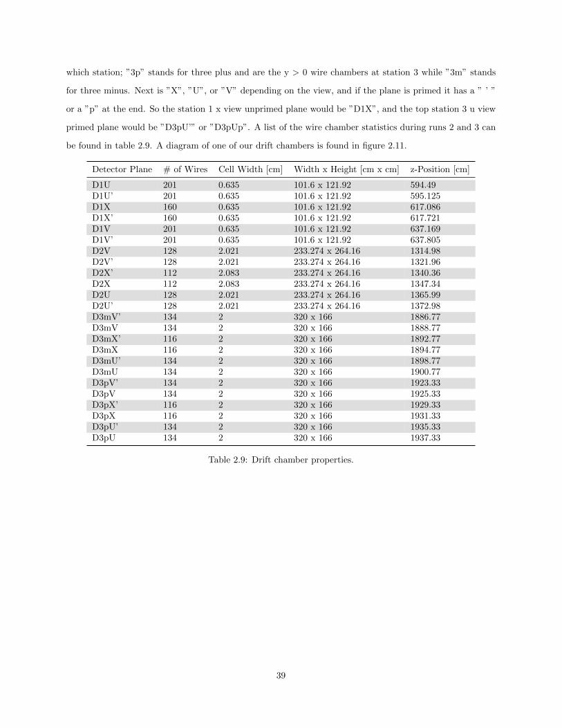
which station; ”3p” stands for three plus and are the y > 0 wire chambers at station 3 while ”3m” stands

for three minus. Next is ”X”, ”U”, or ”V” depending on the view, and if the plane is primed it has a ” ’ ”

or a ”p” at the end. So the station 1 x view unprimed plane would be ”D1X”, and the top station 3 u view

primed plane would be ”D3pU’” or ”D3pUp”. A list of the wire chamber statistics during runs 2 and 3 can

be found in table 2.9. A diagram of one of our drift chambers is found in figure 2.11.

Detector Plane # of Wires Cell Width [cm] Width x Height [cm x cm] z-Position [cm]

D1U 201 0.635 101.6 x 121.92 594.49D1U’ 201 0.635 101.6 x 121.92 595.125D1X 160 0.635 101.6 x 121.92 617.086D1X’ 160 0.635 101.6 x 121.92 617.721D1V 201 0.635 101.6 x 121.92 637.169D1V’ 201 0.635 101.6 x 121.92 637.805D2V 128 2.021 233.274 x 264.16 1314.98D2V’ 128 2.021 233.274 x 264.16 1321.96D2X’ 112 2.083 233.274 x 264.16 1340.36D2X 112 2.083 233.274 x 264.16 1347.34D2U 128 2.021 233.274 x 264.16 1365.99D2U’ 128 2.021 233.274 x 264.16 1372.98D3mV’ 134 2 320 x 166 1886.77D3mV 134 2 320 x 166 1888.77D3mX’ 116 2 320 x 166 1892.77D3mX 116 2 320 x 166 1894.77D3mU’ 134 2 320 x 166 1898.77D3mU 134 2 320 x 166 1900.77D3pV’ 134 2 320 x 166 1923.33D3pV 134 2 320 x 166 1925.33D3pX’ 116 2 320 x 166 1929.33D3pX 116 2 320 x 166 1931.33D3pU’ 134 2 320 x 166 1935.33D3pU 134 2 320 x 166 1937.33

Table 2.9: Drift chamber properties.

39

Figure 2.11: A diagram of a set of drift chambers in station 3. Most drift chambers have more tightly spacedcathodes in the cathode plane.

40

2.5.3 Proportional Tubes

The proportional tubes in our experiments are planes of tubes each individually filled with gas. The outside

of the tubes are grounded and each one has a positively charged wire running along the center. Each tube

is filled with the same gas that fills our wire chambers and in a similar manner the positions of the hits are

known from the drift times. Proportional tubes are receive their name from the fact that the strength of the

output signal is proportional to the energy of the passing particle. Unfortunately, this only works for lower

energies and the difference in signal strength for different relativistic energies is negligible, so this feature is

not useful in our experiment.

The main role of the prop tubes in our experiment is muon identification. There is a meter of iron

between station 3 and station 4, and the prop tubes are only located in station 4. The meter of iron is

there to absorb hadrons and electrons while letting muons pass through. If there are several prop tube hits

aligned with a track passing through stations 2 and 3 the track is considered to be a muon.

There are four planes of prop tubes in the experiment. In each plane there are two layers of prop tubes,

with the second layer directly behind the first and staggered half a tube width, similar to the primed and

unprimed planes in the wire chambers. Each plane is also divided up into nine modules in sets of 16 tubes

each, containing 8 consecutive tubes in the front layer and 8 consecutive tubes in the back layer. Two of

the planes are aligned horizontally (pointing along the x axis) and two of the planes are aligned vertically

(pointing along the y axis). The prop tube names begin with ”P”, then either a ”1” or a ”2” if they are one

of the first two or last two planes, respectively. Then an ”H” or a ”V” based on whether they are aligned

horizontally or vertically. The prop tube modules also have names that begin with the name of the plane

and appends a number ”1” through ”9”. An ”f” or ”b” is appended if one is only talking about the upstream

or downstream layer, respectively. Diagrams of the labelling can be found in figures 2.12 and 2.13. A list of

the prop tube stats can be found in table 2.10.

Plane Name # of Tubes Tube Width [cm] Width x Height [cm x cm] z-Position [cm]P1H 144 5.08 368.3 x 368.3 2100.7P1V 144 5.08 368.3 x 368.3 2176.6P2V 144 5.08 368.3 x 368.3 2369.1P2H 144 5.08 368.3 x 368.3 2392.2

Table 2.10: Drift chamber properties.

41

Figure 2.12: A diagram of the prop tubes. The labelling for the horizontally aligned prop tubes is shown.

Figure 2.13: A diagram of the prop tubes. The labelling for the vertically aligned prop tubes are shown.

42

2.6 Trigger

Seaquest has a high background to signal ratio and requires a robust trigger system to capture the events

we are interested in while reducing the readout of useless data. The Drell-Yan process is a relatively rare

process and contributes very little of the total number of muons moving through the detector. Additionally,

the targets are all very roughly around 10% interaction length, so most of the Drell-Yan events that reach

the spectrometer are events from the beam dump which we do not want to record. When we trigger on an

event, whether it is one we desire or not, the dead time has a rough average of 150 µs and varies a lot based

on how many hits the DAQ needs to readout. During periods in which the QIE based trigger inhibit is

letting triggers fire, the dead time with our current trigger blocks about 20% of the incoming protons. The

trigger also has to be simple enough that it can output a decision within one µs, which is the amount of

time before the data from an event is readout from the drift chambers. Put together, these factors require

a robust trigger system for the SeaQuest experiment[42].

The main trigger system for the experiment is the FPGA trigger system, and is comprised of several

levels of logic gates. All of the levels use CAEN v1495 6U VMEbus modules. I will call them v1945s for

short. Each module has a TDC, which stands for time to digital converter. The TDCs read the leading

edges of the signals from the hodoscope paddles and store the timing information. The TDCs store many

hits at once for each channel, but only one hit per channel per 16 ns timing bin. The fine timing information

has 1 ns resolution but there is still only one hit stored per 16 ns timing bin. If a second hit arrives from

the same channel in the same bin, the earlier hit is discarded. Also, adjustable, channel specific delays are

applied to the data at this point. These delays are necessary because the hodoscopes are not all the same

distance from the trigger electronics and with ns resolution the distance has a very significant effect on the

timing. The v1495s also each contain an FPGA, which stands for field programmable gate array. The field

programmable part means that the logic gates can be setup by the user. In the v1495s each logic gate can

take up to four inputs and have a single output based on a simple logic operator.

The first level, level 0, uses four v1495s and simply passes the signals from the hodoscopes on unchanged

to level 1 during data taking. When we are not taking data, level 0 is used to perform diagnostic tests of the

trigger. It can be switched to output signals from a pulser instead of signals from the hodoscopes. This pulser

sends user-defined signal patterns to the level 1 module in order to test the response of the trigger logic.

The level 1 trigger uses four v1495s and looks for combinations of hodoscope hits matching ”trigger roads”.

A trigger road is a combination of four hodoscope paddles, one from each of the four hodoscope stations,

that was deemed likely to contain a muon from a Drell-Yan event. The first part of the level 1 trigger uses

a separate AND gate for each trigger road. The outputs from this first step are then combined with OR

43

gates to a smaller number of output channels. Trigger roads from the top half of the spectrometer are kept

separate from trigger roads from the bottom half. Trigger roads for positive tracks are kept separate from

trigger roads for negative tracks. The output channels are also divided by an estimate of the x momentum

of the track but that information is not used in the dimuon trigger. The set of all valid trigger roads is

called a roadset. The roadset has changed several times over the course of the experiment. The level 2

triggers use a single v1495 and looks for combinations of input channels which match its criteria. There are

multiple triggers, most of which are turned on during data taking, most of which are prescaled. A prescale

means the trigger will only take effect 1 out of x times, where x is the prescale number. A list of these

trigger conditions can be found in table 2.11. When a trigger fires, a Common Stop signal is sent out to all

of the TDCs, including the ones for the hodoscopes, drift chambers, and trigger system. When this signal is

received the data stored in these TDCs is recorded by the DAQ.

Trigger Half Charge Momentum NotesFPGA 1 TB +- N/A The standard dimuon trigger which we

use for data takingFPGA 2 TT or BB +- N/A Not used, too many background eventsFPGA 3 TB ++ or - - N/A Same sign trigger used for estimating

combinatoric backgroudFPGA 4 T or B + or - N/A Single muon triggerFPGA 5 T or B + or - > 3GeV High momentum single muon trigger

Table 2.11: A list of the level 2 trigger logic conditions for the FPGA triggers. They are sometimes calledMATRIX 1, MATRIX 2, etc. In the half column, T stands for a track in the top half and B stands for atrack in the bottom half. TB means there needs to be one track from each half.

There are also a handful of NIM triggers that don’t use the logic array. The most important of these

triggers is the NIM 3 trigger, which selects which bucket to record data from at random. This is turned on

at a fairly large prescale during data taking. This is useful for analysing background because all of the other

triggers have a bias towards high background events. It is also useful for analysing the intensity spectrum

of the incoming buckets.

There were some improvements to the trigger system between runs 2 and 3. In run 2, the clocks of the

v1495s were not synchronized with the Main Injector RF-Clock. The hodoscope hits were separated into

16 ns bins in the v1495s, and there could only be one hodoscope hit recorded per channel per bin. Since

these bins were not lined up with the RF-Clock, half of the bin could be closer to one bucket and the other

half to another bucket. Because of this, a hit from one bucket could overwrite a hit from a different bucket,

causing inefficiencies in the trigger and also the detector elements in the recorded data. This would not be

uncommon in high intensity events, as the timing jitter for the largest hodoscope paddles is close to ± 8

ns. For run 3 the v1945s were synchronized to the RF-Clock. The time resolution was increased to 1.177

44

ns and the width of the timing bins in the TDCs were increased to 18.9 ns which is the amount of time

between buckets. This has fixed the issue. Analysers should be aware that there may be a small difference

in recording hits between runs 2 and 3. This thesis has analysed data from both runs 2 and 3.

A lot of care has been put into choosing which trigger roads are programmed into the FPGAs. Simulated

Drell-Yan data from our Monte Carlo, called GMC, was used to estimate what roads would have a high

frequency of signal. Of special interest were the events with high xT values, higher than the region precisely

measured by E866. GMC was also used to simulate where the regions of high background would be and

roads with high background were not used in the trigger even if there was Drell-Yan signal in that region

as crippling dead time had to be avoided. Once an initial set of trigger roads was generated, it was used

to take data, and the data was analysed for hot roads that were generating more dead time than they were

worth. Several of these hot roads were found and turned off to reduce the dead time.

2.7 DAQ

The Data Acquisition (DAQ) systems in SeaQuest are divided into four parts. The Main DAQ responds

to the trigger system and controls the readout of hit information. The Beam DAQ controls the real time

analysis and readout of information from the QIE. The Scaler DAQ controls the readout of counters that

are tallied throughout the spill. The Slow Control coordinates an assortment of miscellaneous scripts that

only need to be recorded once per spill.

The Main DAQ starts with the trigger supervisor, which is a VME (Versa Module Europa, which is a

computer bus standard) crate that receives the trigger signals. If the DAQ is already busy reading something

out, or the trigger inhibit from the beam monitoring electronics is on, then the trigger signal is ignored.

The prescale is also applied at this step, the trigger supervisor keeps track for each trigger how many times

the signal has been received since the last time that trigger fired. If that number is less than the prescale

number and the signal is not ignored due to the beam based inhibit or the DAQ being busy, then the trigger

is accepted. When this happens, the trigger supervisor sends a signal to all of the other VME crates that

are part of the main DAQ. Each VME crate has a CPU called a ROC (read out controller) that handles

the readout of the several TDCs in each crate. When the ROC receives the trigger accepted signal it will

interrupt the normal behavior of the TDCs and start reading out the data collected by the TDCs, one TDC

at a time.

The software that coordinates all of this is called CODA (CEBAF (continuous electron beam accelerator

facility) On-line Data Acquisition), which was developed at Jefferson lab. CODA takes the several separate

45

information streams from all the different ROCs and uses them to build a single event data structure, one

event for each accepted trigger. When CODAs buffer is full or when a run ends the events are written to a

CODA file. A separate piece of software, called the decoda and written by Bryan Dannowitz [43], translates

these files into MySQL schemas. A small sample of the events are uploaded to a MySQL server in real time

in order to provide online monitoring of the hit data so people can keep an eye out for dead or hot channels

and other potential problems.

The Beam DAQ also reads out information when the trigger is accepted and outputs the intensity

information of all buckets within 16 buckets of the trigger bucket to the Main DAQ to be included in its

CODA file. Additionally, it stores all of the intensity information from a single spill and at the end of the

spill analyses it to calculate several spill level quantities relating to the beam. It calculates the total QIE

values for all buckets, the total QIE value of all buckets that occurred while the trigger inhibit was active,

the total value of all buckets that occurred during dead time when the trigger inhibit was not active, and

the duty factor. These quantities are recorded once per spill and are also displayed in the control room for

monitoring. Additionally, a multi-threaded process can record the intensity data for the entire spill to a text

file before the next spill occurs. It is approximately 300 MB of data for a single spill and the collaboration

possesses no software to analyse the files. However, it is good to have such records available just in case they

are needed for debugging something.

The scaler DAQ is governed by a separate instance of CODA software which records data twice per spill,

once at the beginning and once at the end. It records a measure of beam intensity from NM3SEM (NM3 is

the location at Fermilab, and SEM stands for secondary emission monitor). It also, for each trigger, records

the raw number of triggers generated, how many triggers were generated when the beam monitor inhibit

was not on, and how many triggers were accepted by the trigger supervisor. There are also channels that

record rates of hits in the top and bottom halves of all the hodoscope planes, but this data is not included

in the MySQL schemas. Many of these scalers are monitored in real time in the control room. They are also

uploaded to the MySQL schemas.

Slow Control is coordinated by an EPICS(Experimental Physics and Industrial Control System) program

which collects data together from several different sources. Fermilab Accelerator Controls Network (ACNET)

provides some of this information, which includes the status of the magnets and measurements of the beam

intensity which are independent of the Cherenkov counter. These measurements are only on the timescale of

an entire spill but are also well calibrated and do not drift over time. There is also equipment that monitors

environmental information in the experimental hall including temperature, humidity, and pressure. These

environmental quantities are not used in analysis but are recorded so that we would have the capability to

46

debug related time dependent effects in our data. Fortunately, no such effects have been discovered. Target

position is recorded, as well as the temperature and pressure of the liquid targets. The status of the liquid

targets is closely monitored in the control room and alarms will go off if problems occur.

The data taking for all of the DAQs can be stopped and started from an instance of CODA running in

the main control room. It has been the practice of this experiment to stop data taking and start a fresh

data taking run whenever the current file reaches a size around 1 GB. This happens on the order of about

one hour. This is a compromise between stability and how often we lose a spill of data by stopping and

restarting. Each of these files is a single run and has a unique run number. All run numbers for viable data

are four or five digits long. These are not to be confused with the other definition of run for our experiment,

where run numbers are assigned to major sections of data taking that last several months.

2.8 Tracking

The main tracking program for our experiment is called kTracker, which stands for Kalman Tracker as it is

based on a Kalman filter. The tracking for this experiment is a very non-trivial exercise due to the high rates

in our detectors. A balance of efficiency, purity, and computation time all factored into the development of

this tracking program. Another tracking program called Sqerp (SeaQuest Event Reconstruction Program)

is also being developed for purposes of cross checking and refining tracking technique.

The first step in kTracker is to remove artificial clusters of hits. If there are two hits on two adjacent

wires where one of the hits is greater than 90% of half the cell width and the other hit is greater than 40%

of half the cell width, then it is assumed that both hits were caused by a single track moving at an angle. In

this case, the hit with the greater drift distance is removed. This removes approximately 25% of the clusters

in the data.

Another type of hit cluster removal used is a cut on electronic noise. If two hits on two adjacent wires

have times within 8 ns of each other, the hits are considered to be electronic noise and are removed. If a

string of 3 or more hits on adjacent wires have similar times, with an average time difference between hits

of 10 ns or less, then all of the hits are considered electronic noise and are removed. This removes about

15% of the clusters.

The last type of hit cluster removal is delta-ray removal. Clusters that are at least three hits long and

not considered electronic noise have the hits in the middle removed and keep one hit on each end. This is

the only type of hit removal that seems to have a major problem of removing true hits, as leaving out the

delta ray removal improves the rate dependent inefficiency by a lot, as shown in 2.14. Unfortunately, the

47

computational time of running kTracker on all the data without delta ray removal is prohibitive.

In addition to cluster removal, when there are two hits on the same wire in the same event, the later of

the two hits is discarded. This is called after pulse removal and we believe that most of these hits are the

result of electronic reflections and not true hits. Also, all the trigger roads for the event’s hodoscope hits

are calculated and any hodoscope hit that is not on one of these trigger roads is discarded.

Figure 2.14: A diagram of rate dependence after various forms of cluster removal. Delta ray removal has amuch stronger effect than all other cluster removal combined.

After the first step of hit removal are the event quality cuts. Events with high occupancies in any given

wire chamber are removed, as the likelihood of a successful reconstruction is very low and the amount of

computational time given to such an event is very high. The cuts on detector occupancy are listed in table

2.12.

Detector MaximumD1 320 HitsD2 160 HitsD3p 150 HitsD3m 150 Hits

Table 2.12: A list of all the occupancy cuts that an event has to pass in order to be eligible for tracking.

After this stage ”triplets” are built in stations 2 and 3. They are called triplets because they combine

wires from the X, U, and V views. First, hits in the X and X’ planes are combined. Then they are matched

up with possible hits from the U and/or U’ planes. Then they are matched up with hits in the V and/or

V’ planes. Valid triplets have to contain at least four hits and have at least one hit from each of the X, U,

and V views. A rough fit of each triplet that does not use drift distance is done, and the triplet has to point

towards both a hodoscope hit (with a fudge factor because of triplet imprecision) and be on a trajectory

that could have possibly come from the target.

48

After these triplets are generated, combinations of triplets from station 2 and 3 that roughly point

towards each other are fitted. These fits have a more precise trajectory and are requirement to point

towards hodoscope hits in stations 2, 3, and 4, this time without a fudge factor. The requirement to be on

a trajectory that could have come from the target is again checked. Also, it has to point towards enough

prop tube hits, after accounting for multiple scattering in the absorber, to be considered a muon track. If

two partial tracks share at least a third of the hits, the one with the larger χ2 is dropped. At this stage, the

tracker attempts to resolve the left right ambiguity in the wire chamber hits.

While searching for possible cuts, it was noticed that the ratio of two quantities, r1 and r2 shown in

figure 2.15, was close to a constant. Figure 2.16 shows the consistency of this ratio. The kTracker takes

advantage of this by calculating the value of r2 for the partial track and using it to estimate the value of

r1. This estimate is used to generate a narrow window (r1 ± 5cm) of station 1 hits that can be paired with

that partial track. The tracker then resolves the leftover left right ambiguity for each view that has both a

primed and unprimed hit by requiring that the track slope is consistent with the hits. For any views that

only have one hit a χ2 value is calculated for the entire track twice, once with the hit on each side, and the

hit is assigned to the side with the smallest χ2.

Figure 2.15: A diagram of how the sagittas are calculated.

Figure 2.16: Graphs of the sagitta ratio r1/r2 for the X and U views. They peak fairly sharply, enablingthis to be used as a cut early on in the tracking process.

49

Next the track removes bad hits. The hit with the largest residual is removed if the residual between

the track and the hit is greater than three times the resolution of the chamber. The track is then refit.

The process is repeated until no hits have a residual that is greater than three times the resolution of the

chamber. The entire track is dropped if the track no longer fits the basic criteria. The track must still point

to fired x hodoscope paddles in all stations. The track must have at least four hits in all stations and at

least one hit in each view in all stations. The track must be between 5 and 100 GeV, and the deflection in

the absorber in front of station 4 can not be too much larger than expected.

At this stage the tracker uses a method based on the Kalman Filter technique in order to do a more

precise fit of the track compared to the earlier coarse results. The Kalman Filter technique is where one

uses a series of measurements to iteratively update the parameters of a model. At each step the difference

between the model’s prediction and the current measurement, the uncertainties on the measurement, and

the uncertainties of current model’s parameters are used to update the parameters of the model and the

uncertainties of those parameters. Instead of a series of measurements in time, kTracker uses each hit as a

separate measurement to update the model. Once all the hits have been added, it loops back around and

adds the hits again, repeating until the track parameters have converged.

After the Kalman Filter kTracker ”swims” the tracked muon back through FMag to find the origin of

the track. The muon starts at the back end of FMag, with the position and momentum predicted by the

tracker so far. Then FMag is divided up into slices and the muon is swum through each slice. In the first

half of the slice, half of the energy loss is applied, although since the simulation is going backwards in time

it is in one way an energy increase. Then the pT kick for that slice is applied in the middle of that slice,

and then the other half of the energy loss is applied. Kun found that the tracker is most accurate when the

peak value for the energy loss is used, not the mean value. The position where the track comes closest to

the beam line is considered the origin of the track.

If the tracker discovers two tracks that both come from the target, or two tracks that both come from

the dump, the tracker attempts to calculate the properties of the dimuon. Both tracks are assigned the

same origin, which is based on the z position during the tracking step in which the two tracks came closest

to intersecting. The tracks are then recalculated using the same Kalman Filter and swimming process as

before but with their origin fixed. The resulting track parameters are then used to calculate the momentum

and invariant mass of the dimuon.

50

2.9 Production Overview

The data in this experiment is organized at the highest level by which roadset it belongs to. A handful of

cuts are roadset dependent and so it is convenient to separate our data by roadset for analysis purposes.

After the data is tracked the reconstructed tracks and dimuons for the entire roadset is copied into a

single MySQL schema, along with spill and event level information. Hit level data is not copied into

these schemas. These schemas are named merged_roadset###_R###_V###. The roadset number identifies

which block of data is stored in the schema, while the R### part is the major software version number.

The V### part is the minor software version number. The biggest changes when going to a new software

version are usually in the tracking software. All of the merged productions can be found on all of the

MySQL servers: seaquel.physics.illinois.edu, e906-db1.fnal.gov, e906-db2.fnal.gov, and e906-db3.fnal.gov.

The version analysed in this thesis is R005 V001 and the roadsets analysed are 57, 59, 62, 67, and 70.

All of the individual runs that make up a roadset are also stored on the MySQL servers, but each run

is only on one server under most circumstances. Each run has an individual schema with the schema name

Run_###### where ###### is the run number. These schemas do store hit level information that would be

impractical to store in the merged schemas as the table size would go over a TB.

Spill level data, which is data that is only recorded once or twice a spill, is stored in several different

tables. These tables include Spill, BeamDAQ, Beam, Target, and Scaler. The Spill table contains the

liveProtons field, which is the number of protons that struck the target that spill while the trigger was not

inhibited and the DAQ was not unavailable due to reading out data. It also contains the dataQuality field,

which is 0 if the Spill passed all of the Spill level cuts. The number in the field indicates which cuts were not

passed. The BeamDAQ and Beam tables contain mostly information about the beam and the Target tables

contain a lot of information about the Target. The Scaler table contains counts of how often a given event

happened during a spill, such as a Matrix1 or NIM3 trigger. Unfortunately these tables are organized in an

unintuitive manner, such as magnetic field strength information in the Beam table. The Analysis section of

this thesis documents where each variable that is used in the data quality cuts can be found and what it

means.

The event level tables are Event and QIE. The Event table contains information about which trigger

conditions were met, and the QIE table contains information about the number of protons in the triggering

bucket as well as the 16 buckets before and after the triggering bucket. The QIE table is indispensable to the

rate dependence analysis. Again, all cuts on fields in these tables are documented in the Analysis section.

The kTrack and kDimuon tables are also event level tables, but they contain reconstructed information

as opposed to raw data. These tables could change significantly between software versions while the other

51

tables wouldn’t. The kTrack table contains tracks that are reconstructed by kTracker, and the kDimuon

table contains reconstructed dimuons. Again, all cuts on fields in these tables are documented in the Analysis

section.

52

Chapter 3

Monte Carlo

The Monte Carlo used in this experiment is called GMC, for Geant4 Monte Carlo. It is based off of FastMC,

which is the Monte Carlo used in the previous experiment adapted to the spectrometer and beam energy

of this experiment. The Monte Carlo has been used to estimate where the background noise would be

concentrated during the commissioning step of this experiment. It was used in the initial development of

trigger roads to estimate which roads had acceptable signal to background ratios and also to determine

which roads had high value high xT dimuons. It also is used extensively in refining kTracker to produce

more accurate results, since unlike data, we know the results that tracking should arrive at when used on

Monte Carlo. It is also used to develop cuts used to separate background and signal, such as the target

dump separation cut. When mixed with the NIM3 random triggers from data before being run through

kTracker, it provides a measure of the intensity based drop in efficiency.

3.1 Generators

In order for Geant4 to simulate anything, one or more particles have to be generated at the start of each

event. The code for this resides in the GeneratePrimaries() function of the PrimaryGeneratorAction.cc file.

Based on the settings given to GMC at runtime it will use either the gun generator or dimuon generator.

In either case, at the end of the function at least one particle will be given to Geant4 to be tracked through

the spectrometer. When a particle is given to Geant4 it needs a particleID (i.e. 11 for electron), a position,

and a momentum.

3.1.1 Gun Generator

This should be thought of as the background generator, but the name gun generator has stuck. This is a

very simple generator that creates a proton on the beam axis in front of the target with 120 GeV momentum

towards the target. Unfortunately this is not a very efficient generator for simulating background as our

experiment has a high rate of incoming protons but very few actually generate particles that make it through

53

to the detectors. A large number of instances of GMC running in parallel for long periods of time is necessary

to generate a reasonable set of data.

This generator was good for estimating where the hot areas were going to be while the experiment was

being commissioned. It has limitations though for estimating false positives in the background signals.

While tracking particles through the spectrometer Geant4 will simulate common results of these particles

colliding with materials. However Geant4 is not intended to simulate more rare interactions such as the

Drell-Yan process, and some of these more rare interactions are significant enough to change the details of

the results, especially since the more common interactions have difficulty getting a muon out of the iron

magnet. Combined with the low efficiency of the generator it is much faster and a little more accurate to

just use the NIM3 random triggers as a background sample.

3.1.2 Dimuon Generator

The dimuon generator is in one sense three generators, as it can generate Drell-Yan dimuons, J/Ψ dimuons,

or Ψ’ dimuons. The three options share a lot of code. If the J/Ψ or Ψ’ option is chosen, the invariant mass

of the dimuon is set accordingly. Otherwise the mass is picked from a flat distribution, usually from 2 to

10 GeV. xF is also picked from a flat distribution from -1 to 1. These values are used to calculate xb and

xt, according to equation 4.7. Equation 3.1 is used to pick pT from a weighted distribution based on the

measured pT distribution of Drell-Yan dimuons[44]. cos(θ) is picked from a weighted distribution according

to 1 + cos2(θ) if it is Drell-Yan or from a flat distribution if it is from a J/Psi, and φ is picked from a flat

distribution. The angles are the muon angles in the Collins Soper frame.

w(pT ) =pT

(1+(pT /3)2)6(3.1)

The invariant mass and the angles give us the 4-momentum of the two muons in the Collins Soper frame,

but Geant4 needs the momentum to be in the lab frame. The Collins Soper frame is Lorentz boosted in

both the pT and beam line direction and is also rotated in comparison to the lab frame. First, in order

to calculate the rotation needed, the momentum of both the target proton and beam proton in the proton

center of mass frame are Lorentz boosted twice, once along the beam line direction and once along pT , to get

the results in a dimuon rest frame. Then the angle of both protons with respect to the beam line are summed

and divided by two to get the angle of the line that bisects the beam proton momentum and the negative

target proton momentum. With this angle, the 4-momentum of the two muons is rotated back to the lab

frame rotation, then Lorentz boosted opposite the pT direction, then Lorentz boosted to the proton-proton

c.m. frame, then Lorentz boosted to the lab frame. Of course the three Lorentz boosts could be combined

54

into a single boost but it seemed simpler code wise to do it in three simpler boosts.

A weight needs to be calculated for the event based on the kinematic variables in the equation. Since the

invariant mass and xf are picked from a flat distribution rather than one weighted according to the cross

section, simply treating all events generated by the Monte Carlo equally will result in drastically inaccurate

results. The likelier events need to have a larger weight when doing any sort of analysis. The Drell-Yan

events are weighted according to equation 1.17, multiplied by the K factor. This cross section is multiplied

by a value I call nucleons per area, which is the nucleon density of the target multiplied by the length of

the target. The length of the target is reduced slightly to correct for beam attenuation. It is also multiplied

by the beam current, which is 2e12 protons per second. This is because the Monte Carlo was designed to

determine things such as number of tracks per second, number of hits per second, number of events per

second etc. rather than a cross section. To correctly account for the range in mass and range in xF of

acceptable events, it is also multiplied by (Mmax −Mmin)(xF max − xF min). To determine the number of

dimuons per second fitting any criteria, the weights of all events fitting this criteria are summed up, then

divided by the number of events thrown by the generator.

The weighting for the J/Ψ and Ψ’ are different. The pT distribution is taken from Measurement of

J/Ψ and Ψ’ production in 800 Gev/c proton-gold collisions[31]. The cross section is also taken from the

same source and the branching ratio into µ+µ− from Particle Physics Booklet [45]. They also have the same

modifications by nucleons per area and beam current, and the rates of dimuons per second are calculated in

the same fashion.

3.2 Physics List

Geant4 provides several prebuilt physics lists that contain a best guess at what physics experiments might

need to include in their simulations. Originally it was our intent to build a physics list from processes

and particles provided by Geant4 instead of using one of the prebuilt lists. The first versions of GMC

did use such a list compiled by my predecessor and I had hoped that the gun generator might gain some

performance by not including processes that were unnecessary. When we needed to upgrade Geant4 though

it became impossible to ensure that such a user built list had everything we needed due to undocumented

changes in the names of several processes and other poor Geant4 documentation. Using the internet[46]

for guidance it appeared that the FTFP BERT physics list was a good default choice for our energies. We

went with FTFP BERT EMX, although in retrospect the tweaking to the default EM settings by including

the EMX was completely unnecessary. We didn’t see the need to include any processes in addition to the

55

FTFP BERT EMX list.

3.3 Geometry

There are two parts to the geometry of the experiment that is implemented in GMC. The first part contains all

the information needed to be given to GMC to simulate the movement of particles through our spectrometer.

Geant4 uses several objects to contain the information used in simulating the spectrometer. The G4Material

object contains the information Geant4 needs to simulate a material, which is its density and the list of

elements in the material and the percent of the material’s mass each element makes up. The G4VSolid

objects contain information about a shape and its dimensions. The G4LogicalVolume object combines a

solid with a material and includes the information of whether or not the volume is a detector. Each logical

volume is attached to one or more physical volumes which contain the position and orientation of each

piece of the spectrometer[47]. The magnetic fields are also part of the information given to Geant4 for the

simulations. The magnetic field files for FMag and KMag are grids of x, y, and z positions with x, y, and

z field strengths. The strength at any given point is determined by interpolating between the eight closest

vertices of the grid, which form a cube around the point.

The MySQL servers all have a copy of the latest geometry files in which this information is kept. The

names of the geometry schemas are of the form geometry_G##_run#. There is a separate geometry for each

run as detectors have been added, moved, and replaced between runs. The geometry schemas have required

constant updates as bugs are fixed and more precise detector survey and alignment information is available;

the number after G is the revision number of the geometry. Old versions of the geometry are kept available

so that in progress studies can be finished without losing reproducibility. These schemas have several tables,

one each for the material, logical volume, and physical volume objects, and several for the different variations

of solid objects (cylinders, rectangular prisms, etc.). There are also a couple of tables for the magnetic fields,

although these are typically loaded from tab separated ASCII files instead. These files are located in the

geometry/magnetic fields/ folder of the SeaQuest Software Distribution.

The other part of the geometry is the part that doesn’t get loaded into the Geant4 part of the simulation

but are still loaded into GMC to help interpret the information that Geant4 returns. The Planes table in

the MySQL geometry schemas connects all of the Physical Volumes used in the simulation to the actual

planes of the experiment. This table holds the information of how many detector planes are within each

Physical Volume, the coordinates of the center of the plane, its rotation, how many wires are in the plane,

what the spacing is between wires, the rotation of the wires with respect to the plane, and how much the

56

center wire is offset from the center of the chamber. For the hodoscopes it contains how much the paddles

overlap each other. The positions and rotations of the planes in this table are determined by surveys done

by Fermilab. These positions and rotations are used as input into calculating an even finer alignment by

tracking results from special data taking runs where KMag was turned off. Such special runs have straight

tracks through all of the detectors which makes alignment much easier. These alignment results are stored

in the PlaneOffsets table in the MySQL geometry schemas. The Planes and PlaneOffsets tables combined

allow GMC to calculate which wires, paddles, and tubes are struck when a simulated particle passes through

a simulated detector, as well as calculating a drift distance. Other relevant detector information is stored

in text files in /GMC/code/sqlTables/ which are uploaded to the GMC output schema at the beginning of

the run. The hodoInfo.tsv and chamberInfo.tsv tables link each wire, paddle, and tube to a rocID, boardID,

and channelID. These IDs identify which channel of the DAQ electronics are connected to which detector

element. The RT.tsv table contains the information which maps the drift distance to drift time for our wire

chambers and prop tubes.

3.4 Output

All of the output of GMC is put into a MySQL database. The amount of information uploaded for a single

instance of GMC is low compared to its run time, so it is easily possible for many parallel instances of GMC

to be simultaneously running and uploading information to a single MySQL server. For each table that

GMC uploads, it packages together many rows into a single upload query, and then uploads it in one query

once a threshold is reached before starting on a new query. This avoids the traffic jam of tens of GB being

uploaded at once, which is undesirable. It also avoids a different possible traffic jam of bogging down the

MySQL server in the massive overhead generated by putting each uploaded row into a separate query.

Some of the tables are Monte Carlo truth tables and are prefaced by an m, for tables such as mHit or

mTrack. These tables are not used as input to kTracker, but are used to compare the output of kTracker to

the truth values to see where adjustments in the tracking algorithm are needed. For example, the mHit table

will contain the momentum of the particle when it struck the detector, information that is not available in

real data. GMC will also contain other tables, such as Hit, which mimic the data structure of real data and

lack this truth data. These tables are the ones used as input by kTracker.

One of the most important tables is the mRun table, which has a single row for each parallel instance of

GMC in that production. In this row all of the settings used in that run are detailed, such as which PDF

set was used, magnetic field strengths as a fraction of the field files, kinematic ranges for x and mass, and a

57

variety of other settings.

The other important truth tables are the mTrack, mDimuon, and mHit tables. The mTrack table contains

the tracks momentum and position at the origin and the first and third detector stations, its particleID,

which hodoscope, wire chamber, and prop tube stations it hit, and if it isn’t a primary particle it contains the

trackIDs of the parent and the Geant4 process that created it. The mDimuon table contains the kinematics

of the dimuon, such as invariant mass, xF , xB , xT , and its Collins-Soper angles. It contains the position

and momentum it had at its origin. It also contains trackIDs for the positive and negative muons. It also

contains the weight for the dimuon. The mHit tables contain the position and momentum of the particle

where it intersected the detector, its true drift time, and which track it belongs to.

Most of the non-truth tables are provided by kTracker, which provide results in kTrack and kDimuon

to compare to the Monte Carlo results. The Hit table, however, is provided by GMC, and contains only

information that would be found in the real data. In addition, kTracker has a function that will make

random changes to the drift time and distance of each Hit entry to match the uncertainties generated by

the finite resolution of our detectors, while mHit keeps the true information.

The output name of the MySQL productions that determine this information are as

mc_[generator]_[target]_M###_S###. The generator is a name like drellyan, jpsi, or gun to indicate which

generator is used. The target is the name of which target was used, like C for carbon. If the dimuons have

their origin in the beam dump then it says dump instead. The M number is the revision number for GMC,

and there is a table on the Fermilab Redmine page for the Seaquest Monte Carlo that links that version

number to the github hash for that commit, as well as supplying some small comments on what was changed.

The S number is used to distinguish between multiple GMC productions that have different settings but

would otherwise have the same name.

3.5 Running GMC

Creating a GMC production requires the use of a couple of helper programs. First, the TableLoader table

is run, which takes a geometry file and some tab separated text files and processes them into tables used

by GMC in its MySQL schema. This takes time on the order of several minutes. Then, the GMC program

itself is run. It takes a little less than a day to generate about 3,000 dimuons in the spectrometer acceptance

and or about a single spill’s worth of protons. The MySQL servers can handle a few hundred parallel GMC

productions, give or take based on what else is using the server. Each parallel instance of GMC generates

separate tables, a collection of parallel instances will generate tables named Event 1, Event 2, Event 3,

58

etc. After all the GMC instances finish running, the TableMerger program should be run. This merges

the tables together so there is only one Event table, one mDimuon table, etc. It also removes any rows

from any run that did not finish running and creates the indices on the finished tables. This takes about 2

days to complete. TableLoader and TableMerger both give a list of possible run time arguments with the

-h argument. Both programs will need a MySQL login, MySQL password, and GMC schema name, and

TableLoader will need a geometry schema name.

The easiest way to run a single instance of GMC is to give it a macro file at runtime with the -m argument,

such as ”GMC -m file.mac”. The macro file is simple a text file with each command on a separate line in order.

The easiest way to run many instances is on the Fermilab seaquestgpvm machines, using the runGMC.py

program. ”runGMC.py -h” will list the options for running it. When run, it will run TableLoader first

before submitting the GMC runs as jobs to Fermilab’s grid computing system. TableMerger still has to be

run separately by the user once all the jobs have finished.

3.5.1 Commands

A full list of the commands is on the wiki on the Fermilab Redmine page for the Seaquest Monte Carlo. The

important commands are listed in table 3.1.

3.6 GMC Improvements

When I joined this experiment, I was tasked with running, maintaining, and improving GMC, and getting

it to work on our systems. While I did not write the initial code, it has gone through so many iterations

that I have written the majority of the code that currently makes up the program.

One of the first major changes that was made was changing the geometry from hard coded instances

of each detector to loading it from MySQL schemas. This made the geometry much more human readable

and the code much more manageable. It is a good rule of thumb to store information used in a program in

input files outside of the code so that these parameters can be edited easily by people unfamiliar with the

code and so that multiple input options can be maintained without bloating the code. It also lets programs

analysing the output of GMC understand the geometry, it would be completely impractical to have such

programs parse the GMC code for those parameters.

Another early major change was the digitization of the hits. Early output of GMC just had a position

and detector name of each hit, and the position was a general position and not relative to the center of

the detector. By loading in survey information for each detector I could find the intersection between the

59

Command Argument Explanation

/control/server string Name of the MySQL server to write the output to./control/login string MySQL login/control/password string MySQL password/control/outputFile string Name of the MySQL schema to write the output

to./control/geometrySchema string Name of the MySQL schema to fetch geometry info

from./set/eventGenType enum(gun, dimuon) Which generator to use./set/dimuonSource enum(DY, JPsi,

Psi Prime)Process that generates dimuons.

/set/eventPos enum(target, dump,upstream, all)

Location of dimuon origin.

/set/target int Sets the target material./set/FMagMultiplier double Multiplies the field in the magnetic field file for

FMag. Important for simulating a flipped polarity.The values used are typically not exactly one andare based on the magnet calibration.

/set/KMagMultiplier double As above, but for KMag./set/recordMethod enum(hits, dimuon-

Full, dimuonOnly)The hits option makes it so tracks that cause atleast one hit are recorded. The dimuonFull optiononly records events where both muons are withinspectrometer acceptance. The dimuonOnly optionrecords no tracks, only initial kinematics for alldimuons.

/control/initialize none Initializes some Geant4 objects. Required, secondto last command.

/run/beamOn int How many protons or dimuons to generate. Re-quired, last command.

Table 3.1: Table of GMC commands.

60

particle’s line and the plane of the detector[48]. I could then get the relative position of the hit in the plane,

and calculate which wire, paddle, or tube was struck and the drift distance. With the association of DAQ

channelIDs, drift times, detector elementIDs, and drift distances to each hit I was able to provide a data

format mimicking the experiment’s data format so that analysis programs could easily be run on both real

data and simulated data.

Another problem I worked on was the unexpectedly small number of hits in the edges of the detectors

in the x direction in gun generator mode. We were expecting the magnets to push most of these particles

to the edges so it was surprising to see two peaks closer to the middle of the detector, one on each side.

Eventually I found that the culprit was an optimization cut that tried to make the inefficient gun generator

more efficient. It cut particles that were travelling at a large angle under the presumption that these particles

would miss the detectors. I removed this cut and the simulation matched what we expected, but then the

run speed slowed to a crawl. I changed the cut to remove particles moving backwards through the magnet,

and this gave accurate results at a slower but manageable run speed.

Another project involving GMC was cross checking it against FastMC, the Monte Carlo from the pre-

vious experiment which was written in Fortran, modified to use SeaQuest’s beam energy, and only used

rough calculations for tracking particles through materials. The dimuon generator code in GMC is a C++

translation of the Fortran code used in a section of FastMC. While the tracking in Geant4 is more precise,

FastMC should be just as accurate in generating the initial dimuon kinematics and weighting. However, the

output from FastMC and GMC just wasn’t matching up. We found a few typos but could not track down

where the differences were coming from. The culprit turned out to be different standards of units in Geant4

and the PDFlib libraries. In Geant4, the default unit is MeV, but PDFLib was expecting all arguments

for energy to be in GeV. This resulted in all energy parameters being passed to PDFLib to be multiplied

by 1,000 compared to what they should have been, which caused the PDFs to return much different results

than we expected.

Another improvement I made to GMC was replacing PDFlib with LHAPDF. LHAPDF contains more

recent PDF sets and is also available in C++, while PDFlib is in Fortran and required complications in coding

and the makefile to have the C++ and Fortran interface which made it harder to consistently compile in

multiple environments. This improvement also made things more human readable with the all of the code

involving Drell-Yan physics being in the same place.

61

3.7 MySQL Usage

Using a MySQL database to store much of our data, both simulated and real, is much less common than

using ROOT. There were both advantages and disadvantages to this approach, and I believe that a relational

database such as MySQL can have a strong place in physics analysis while not being the answer for everything.

Also, like any software tool, knowledge of how to use it best is important.

The largest problem with using MySQL for everything is that it isn’t efficient for anything that requires

reading in every single row. Above I mentioned that while the magnetic fields can be read in from the MySQL

database, they are almost always read in through the tab separated ASCII files. This is because reading

in the data through the text files is several times faster. For tracking, the hit data(real, not simulated) is

available in ROOT file format as well as MySQL format, and it was found to be much faster to read in the

data from ROOT. In this case every hit needed to be used as input into the tracking program.

Another problem is that MySQL can also take longer to write data. Data coming in from hundreds of

programs running in parallel on grid computing can bog down a MySQL server. This is especially true if

the tables have indices enabled as data is being written to them. If they are disabled while being written to

and enabled after, the building of the indices can take even days depending on the size of data.

Another problem that is less of an issue with today’s hard drive capacities is the extra room that is taken

up by MySQL databases compared to the data structures of a library such as ROOT. MySQL databases

are larger even without indices on the fields, although in practice there will almost always be an index on

at least one field. Typical tables will have multiple indices and these indices can take up space comparable

to the raw data. Our data storage has reached the level of Terabytes, and space has sometimes become a

bit tight on our MySQL servers.

One of the great things about MySQL is how quickly and easily you can fetch information that requires

cutting on some condition. If you cut on an indexed field it greatly reduces the amount of data that has

to be read. Queries are also quicker than writing a program to loop through data to get what you want,

when you need to ask a lot of questions about the data these savings in human time add up. For example,

a flat file is better for reading in the entire magnetic field, but if you wanted to ask MySQL what the

field in the y direction is integrated over a line through the beam axis, you could just type in ”SELECT

SUM(By)*(MAX(z) - MIN(z))/(COUNT(1) - 1) FROM FMag WHERE x = 0 AND y = 0” and the answer

pops up on your screen, while retrieving the information from a flat file would take longer.

Another advantage of MySQL is that it is well documented and easy to learn. The official documentation

is detailed and extensive and there are a ton of articles to be found online giving advice on optimizing

performance and if you have an issue you can almost certainly find a question on Stack Exchange where

62

someone else has had your problem before.

Yet another advantage is that MySQL is supported by almost all programming languages. There are

code libraries for interfacing between MySQL and C++, python, java, ruby, and others. Many programs,

such as ROOT, have an interface for MySQL. Whatever someone prefers to use, odds are they can connect

to MySQL with it without much fuss.

In order to use MySQL optimally both the person managing the database and the person writing the

queries need to know good practices with indices. The person managing the database needs to know which

fields should be indexed to save query time, and which fields would do nothing other than slow writing time

and bloat data size if indexed. The person writing the queries needs to know how to check which fields are

indexed, which is quick and easy, and also how to write a query to take advantage of these indices. Also,

anyone who reads from or writes to the database using a program should absolutely not read or write a

single row at a time, as there is overhead in network time for every query that becomes significant if one tries

to submit stupidly large numbers of queries per second. Learning how to write MySQL queries is similar to

learning how to write a programming language, you won’t get much out of MySQL if you don’t know how

to do a JOIN like you won’t get much out of C++ if you don’t know how to write a for loop. Often the

penalty for a poor query in MySQL isn’t an error message from bad syntax, but a query that runs for orders

of magnitude longer than necessary.

63

Chapter 4

Analysis

There are several steps in the extraction of σpd/2σpp from the data. First a lot of cuts have to be made

on the spill data and the reconstructed dimuons to ensure that the data is accurate. There are several

separate rate dependent corrections to be made based on the tracking efficiency, background subtraction,

and miscellaneous rate dependence. There is also a correction to be made for 1H contamination in the 2H

target. Once σpd/2σpp is known then the value of d/u can be calculated through an iterative procedure.

4.1 Kinematic Variables

Before we even start talking about cuts we need to explicitly define how we calculate the quantities we are

cutting on. For most variables it is straightforward, but for Bjorken x and Feynmann x we need to be clear

on how we calculate them since there are multiple equations that can be used. The calculation of Bjorken

x in particular is far from straightforward.

Feynmann x, or xF is defined as q‖/q‖max, where q‖ is the longitudinal momentum of a particle. The

particle in our case is the virtual photon in the Drell-Yan process. xF is sometimes written as 2q‖/√s, but

this ignores the mass of the virtual photon, which should be taken into account. We choose to use equation

4.1 as our definition of xF , which is the other common form of xF .

xF =2q‖√

s−M2/√s

(4.1)

Bjorken x, which I will often shorten to just x, is commonly defined as the ratio between the parton’s

momentum and its proton’s momentum when boosted longitudinally to an infinite momentum frame. If

we boost something with momentum ~p to its infinite momentum frame it will have momentum ~p′. p′‖ =

γ(p‖ + βp0), so the momentum fraction x of a parton of momentum ~k and its proton of momentum ~P is

then equation 4.3.

x =γ(k‖+βk0)

γ(P‖+βP0)(4.2)

64

Infinite momentum frame, β = 1.

x =(k‖+k0)

(P‖+P0)(4.3)

We can not measure the longitudinal momentum of a single parton involved in the Drell-Yan reaction,

so we can not calculate x directly. We have to estimate the value of x by using one of several formulas,

equations 4.4 through 4.7, which assume that the mass and p⊥ of the parton are negligibly small.

xA =Q2

2 ~PA·~q(4.4)

x =

√τ +

x2F4± xF

2(4.5)

x =√τe±y (4.6)

xA =~PB ·~q~PB · ~PA

(4.7)

τ is equal to M2/s, and y is the rapidity equal to 0.5ln((q0 + q‖)/(q0 − q‖)). If a formula has a ±, then

the + is for calculating x for the beam and the − is for calculating x for the target. The fourth definition,

equation 4.7, uses the momentum of both protons in the equation so they get A and B subscripts to tell

them apart. Clearly this last calculation can not be used in certain experiments, such as DIS.

As an example I will demonstrate how the first example reduces to x in this approximation. I will do

this for the beam parton and work in the center of mass frame. Using k for the beam parton momentum

and j for the target parton momentum,

x =Q2

2~P ·~q(4.8)

Q2 = k20 + j2

0 + 2k · j (4.9)

Q2 = 2(k0j0 − k‖j‖) (4.10)

k0, j0, and k‖ are all positive, but j‖ is negative. Where parton mass and pT are zero k0 is equal in

65

magnitude to k‖.

Q2 = −4k‖j‖ (4.11)

Now for the denominator.

2~P · ~q = 2P0q0 − 2P‖q‖ (4.12)

2~P · ~q = 2P0(k‖ − j‖)− 2P‖(k‖ + j‖) (4.13)

2~P · ~q = 2P0((1−P‖P0

)k‖ − (1 +P‖P0

)j‖) (4.14)

2~P · ~q = −2P0(1 +P‖P0

)j‖(1− (1−P‖P0

)k‖j‖

) (4.15)

Putting it together.

Q2

2~P ·~q=

−4k‖j‖

−2P0(1+P‖P0

)j‖(1−(1−P‖P0

)k‖j‖

)

(4.16)

Q2

2~P ·~q=

2k‖

(P0+P‖)(1−(1−P‖P0

)k‖j‖

)

(4.17)

Using the approximation 11−z = 1 + z where z << 1, and the fact that 1− P0

P‖is very close to 0.

Q2

2~P ·~q=

2k‖P0+P‖

(1 + (1−P‖P0

)k‖j‖

) (4.18)

Q2

2~P ·~q=

k0+k‖P0+P‖

(1 +P0−P‖P0

k‖j‖

) (4.19)

Q2

2~P ·~q= x(1 +

P0−P‖P0

k‖j‖

) (4.20)

P0 ≈ P‖, and if one treats the difference as negligible then equation 4.20 becomes equation 4.3. Now

this is almost equal to the momentum fraction x, as P0 ≈ P‖, but the equation can be improved. If instead

of using the proton’s 4 momentum, we used a different vector that is similar, we could end up with an

66

equation exactly equal to x when ignoring the parton p2T terms. This new vector, ~P ′, would need to have

P ′0 +P ′‖ = P0 +P‖ so that the (k0 +k‖)/(P0 +P‖) part of equation 4.19 is properly equal to x. Also, P ′0 = P ′‖

so that theP0−P‖P0

k‖j‖

in equation 4.20 reduces to 0. The vector ~P ′ = (P ′, 0, 0, P ′), where P ′ = (P0 + P‖)/2,

meets both these conditions. So I modified equation 4.4 to use ~P ′ instead of ~P . This changes equation 4.20

to equation 4.22, giving us a more accurate way of calculating x.

Q2

2 ~P ′·~q= x(1 + 0

P0

k‖j‖

) (4.21)

Q2

2 ~P ′·~q= x (4.22)

After working out the other formulas in equations 4.5 through 4.7 I also replaced all instances of τ with√M2/4P ′2, all instances of xF with q‖/P

′, and all other instances of ~P with ~P ′.

If the parton mass and pT are equal to zero then these new formulas are equal to one another. However,

in our data, p⊥ of the parton is not always negligibly small and the choice of formula can actually have a

significant effect on the resulting calculation of x. It is still negligible at pT < 1GeV , with the differences

in the various definitions being in the range of about 0.001 and 0.002 for xT . At high pT the differences

between equations 4.4 and 4.7 were the largest, with the difference being about 0.02 for xT at pT between

1.5 and 2 GeV, which is enough of a change to shift results to another bin in x at low x. The differences in

xB are much more pronounced, being about 0.07 at pT between 1.5 and 2 GeV. This is significant enough

that some care and attention to the choice of formula is deserved.

So in order to figure out which formula for x should be used when the parton momentum is not known

and the parton p⊥ is not negligible, I tried write the formulas for x out to quadratic terms in p⊥. I used

approximations with the assumption that p2⊥ << p2

‖ and that quark mass = 0. For each formula that

approximates x I algebraically transformed the formula into a part equal to the right side of equation 4.3

plus some p2⊥ terms. I then estimated which formula would have the smallest p2

⊥ terms in our kinematic

regime. As an example, I will derive the result for equation 4.4 for the beam parton, starting with the Q2

portion,

Q2 = k · k + j · j + 2k · j (4.23)

Q2 = 2k0j0 − 2k⊥ · j⊥ − 2k‖j‖ (4.24)

67

k0 =

√k2‖ + k2

⊥ (4.25)

k0 = k‖

√1 + k2

⊥/k2‖ (4.26)

Using the approximation√

1 + z ≈ 1 + z2

where z << 1.

k0 = k‖(1 +k2⊥2k2‖

) (4.27)

k0 = k‖ +k2⊥2k‖

(4.28)

Since j‖ < 0

j0 = −j‖ −j2⊥2j‖

(4.29)

Q2 = −2(k‖ +k2⊥2k‖

)(j‖ +j2⊥2j‖

)− 2k⊥ · j⊥ − 2k‖j‖ (4.30)

Dropping terms of p4⊥

Q2 = −k‖j2⊥j‖− j‖

k2⊥k‖− 2k⊥ · j⊥ − 4k‖j‖ (4.31)

Q2 = −4k‖j‖(1 +k‖·j‖2k‖j‖

+k2⊥4k2‖

+j2⊥4j2‖

) (4.32)

Now for the 2 ~P ′ · q portion.

2 ~P ′ · q = 2P ′(k0 + j0 − k‖ − j‖) (4.33)

2 ~P ′ · q = 2P ′(k2⊥2k‖− 2j‖ −

j2⊥2j‖

) (4.34)

2 ~P ′ · q = −4P ′j‖(1−k2⊥

4k‖j‖+

j2⊥4j2‖

) (4.35)

Using the approximation 11−z = 1 + z where z << 1.

68

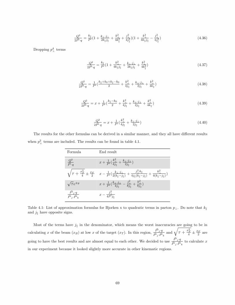
Q2

2 ~P ′·q=

k‖P ′

(1 +k⊥·j⊥2k‖j‖

+k2⊥4k2‖

+j2⊥4j2‖

)(1 +k2⊥

4k‖j‖− j2⊥

4j2‖) (4.36)

Dropping p4⊥ terms

Q2

2 ~P ′·q=

k‖P ′

(1 +k2⊥

4k‖j‖+

k⊥·j⊥2k‖j‖

+k2⊥4k2‖

) (4.37)

Q2

2 ~P ′·q= 1

P ′(k‖+k0+k‖−k0

2+

k2⊥4j‖

+k⊥·j⊥

2j‖+

k2⊥4k‖

) (4.38)

Q2

2 ~P ′·q= x+ 1

P ′(k‖−k0

2+

k2⊥4j‖

+k⊥·j⊥

2j‖+

k2⊥4k‖

) (4.39)

Q2

2 ~P ′·q= x+ 1

P ′(k2⊥4j‖

+k⊥·j⊥

2j‖) (4.40)

The results for the other formulas can be derived in a similar manner, and they all have different results

when p2⊥ terms are included. The results can be found in table 4.1.

Formula End result

Q2

~P ′·qx+ 1

P ′(k2⊥4j‖

+k⊥·j⊥

2j‖)√

τ +x2F4± xF

2x− 1

P ′(k⊥·j⊥

2(k‖−j‖)+

j2⊥k‖4j‖(k‖−j‖)

+k2⊥

4(k‖−j‖))

√τe±y x+ 1

P ′(k⊥·j⊥

4j‖− j2⊥

8j‖+

k2⊥8j‖

)

~P ′j ·q~P ′j · ~P ′k

x− j2⊥4P ′j‖

Table 4.1: List of approximation formulas for Bjorken x to quadratic terms in parton p⊥. Do note that k‖and j‖ have opposite signs.

Most of the terms have j‖ in the denominator, which means the worst inaccuracies are going to be in

calculating x of the beam (xB) at low x of the target (xT ). In this region,~P ′j ·q~P ′j · ~P ′k

and

√τ +

x2F4± xF

2are

going to have the best results and are almost equal to each other. We decided to use~P ′j ·q~P ′j · ~P ′k

to calculate x

in our experiment because it looked slightly more accurate in other kinematic regions.

69

4.2 Cuts

There are two levels of cuts in this analysis. The first level is the spill level. Spills failing these cuts have

all the events in the spill cut and the protons are cut from the live proton count as well. Tables involved in

these cuts are the Spill, Beam, BeamDAQ, Target, and Scaler tables. The second level is the event level.

Tables for this level of cuts are the kTrack, kDimuon, Event, and QIE tables.

4.2.1 Spill Level

The spill level cuts ensure that the data taking conditions were both normal and accurately recorded.

Conditions such as very low beam intensity, an anomalous magnet current, or an unrealistically high duty

factor can all cause the spill to be cut. These cuts are all found in table 4.2. There are also several spill

ranges that have known problems that make them unsuitable for analysis, these ranges and the reason for

exclusion can be found in table 4.3. The number of spills left after each stage of cuts can be found in table

4.4.

A type of cut that can be found for almost every table is the no duplicates cut. Some tables, such as the

Spill table, should only have one entry per spillID. If there are multiple rows then it is a sign that something

has gone wrong with the data recording, and also it is not possible to tell which of the recorded rows is

correct. Some tables, such as the Beam table, record values in multiple rows for each spill. The name field

contains a string that says what value is being recorded, such as beam intensity if the name is S:G2SEM.

So for a given spillID there would be one row for the S:G2SEM value, one row for the F:NM4AN value, and

one row each for the other values, but there should be no duplicates of both spillID and a name field, such

as two S:G2SEM rows for the same spillID. The Scaler table is similar but has two rows for each value, a

beginning of spill (BOS) value and an end of spill (EOS) value, and the spillType field tells which row is

which.

The targetPos value in the spill table contains an integer that corresponds to the target for that spill. We

have seven targets and the IDs range from 1 to 7, so if the value if outside that range the spill information

is obviously incorrect. The other cut on the spill table, spillID 6= 0, gets rid of spills that were not assigned

a spillID due to incomplete DAQ information.

The only cut on the Target table is that the target ID it records has to match the target ID from the

spill table. This is just to make sure the data is consistent.

The Scaler table cuts on EOS values for TSgo, acceptedMatrix1, and afterInhMatrix1 ensure that the

total number of triggers, the total number of matrix 1 triggers, and the number of matrix 1 triggers that

weren’t during dead time are a reasonable value, respectively. The cut ranges are wide and contain all data

70

Table Value Roadsets Good range

Spill targetPos all [1, 7]

spillID all 6= 0

spillID all no duplicates

Target TARGPOS CONTROL all Spill table targetPos

spillID, name all no duplicates

Scaler TSgo, EOS 57, 59 [1,000, 8,000]62, 67, 70 [100, 6,000]

acceptedMatrix1, EOS 57, 59 [1e3, 8e3]62, 67, 70 [100, 6e3]

acceptedMatrix1, BOS all Entry exists

afterInhMatrix1, EOS 57, 59 [1e3, 3e4]62, 67, 70 [100, 1e4]

acceptedMatrix1/afterInhMatrix1, EOS 57, 59 [0.2, 0.9]62, 67, 70 [0.2, 1.05]

spillID, scalerName, spillType all no duplicates

Beam S:G2SEM all [2e12, 1e13]

F:NM4AN all > 1000

spillID, name all no duplicates

BeamDAQ QIESum all [4e10, 1e12]

trigger sum no inhibit all [4e9, 1e11]

inhibit block sum 57, 59 [4e9, 1e11]62, 67, 70 [4e9, 2e11]

dutyfactor53MHz 57, 59 [15, 60]62, 67, 70 [10, 60]

spillID all no duplicates

kTrack # of rows all > 0

Table 4.2: List of Spill Quality cuts

71

where the beam was normal and the trigger and DAQ were functioning properly. There is a cut that requires

there to be a beginning of spill entry for acceptedMatrix1 that is a check to make sure that data was being

recorded at the beginning of the spill. Partial spills can not be correctly normalized by live proton count so

it is important to exclude them from the data.

The S:G2SEM value in the Beam table is a measure of beam intensity. If it is too low then the beam

was probably not active. Values higher than the cut off indicate a problem recording beam intensity. The

F:NM4AN value measures the current powering FMag and ensures that the magnet was on during the spill.

The QIEsum cut in the BeamDAQ table is a second cut on a measure of beam intensity and also cuts out

many spills where the QIE wasn’t reading out properly. The trigger sum no inhibit, inhibit block sum, and

dutyFactor53MHz cuts all try to ensure that the quality of the beam was normal. The quality of the beam

has a strong effect on how many events can be reconstructed and thus spills with very bad beam quality

should be excluded.

The cut on the kTrack table is to make sure that reconstruction has been run on the spill in question.

Since a typical spill contains over 1,000 kTracks, any spill without a single kTrack means that reconstruction

has not been run on those events.

First spillID Last spillID Reason

303215 310954 QIE readout errors371870 376533 Trigger timing shift378366 379333 Trigger timing shift394287 409540 Data Set 3 commissioning period394287 414555 Deuterium flask filled with LH2416207 424180 Manual target control482574 484924 Magnet flipped compared to rest of roadset 62526201 526364 Bad QIE inhibit timing551030 610059 Middle of roadset 67 reconstruction issues581369 582460 KMag off675814 684041 Gas flow problems in station 1684663 689443 D3p has wrong in time window676242 685765 Trigger timing shift

Table 4.3: List of bad spill ranges. The problems with the middle of roadset 67 have been solved and willnot be excluded from future analysis.

Some of the bad spillID ranges in table 4.3 are straightforward, but some are not. The QIE readout errors

indicate a data taking range where a large number of QIE outputs had zeros in them instead of the correct

value. This makes the QIEsum and live proton counts for these spill ranges incorrect. Trigger timing shifts

cause the in time window for the drift chambers and prop tubes to shift relative to the trigger, causing some

legitimate hits to be outside the in time window and not recorded into the data. During the manual target

control period the sensors for reading out the target position were not working and the target table was

72

not automated. The target positions were written down in the run information and the table was manually

adjusted between runs instead of during runs. I think the opportunity for human error here is high and I

prefer not to include these spills, although other people think that these spills can be reliable if cross checked

with the information from the radiation monitors. There is a period during roadset 62 where the magnet

polarity is flipped compared to the rest of the roadset. This did not lead to good data because each roadset

is designed for a specific magnet polarity. There was also an issue with approximately the middle third of

roadset 67 where the data was reconstructed inaccurately. A fix for this was implemented but it was decided

not to retrack the data since a new improved version of the reconstruction code was going to be run soon

on all of the data. Once the R006 data is ready for analysis and quality checked this spill range should no

longer be cut.

roadset All Complete Liquid or Empty Flask Valid

57 48270 45716 32044 2920759 10239 8565 5914 534362 54736 53269 39176 3607867 117827 112291 81183 7153970 6336 6230 4601 3911

All 237408 224442 162918 146078

Table 4.4: List of number of spills at different stages in the cutting process. All is number of spills in theSpill table outside the ranges in table 4.3. Complete is the number of spills that have entries in all tables,and both EOS and BOS entries in Scaler. Liquid or Empty Flask is the result of requiring that the spill beon LH2, LD2, or the empty flask. Valid is the number of spills left after applying all data quality cuts.

4.2.2 Event Level

Table 4.5 has a list of all the event level cuts. Quality cuts remove reconstructed dimuons that might not be

real dimuons or might not be reconstructed accurately. Target cuts ensure that the dimuons came from the

target. The Drell-Yan cut drastically increases the chances of a dimuon being from the Drell-Yan process,

as opposed to combinatoric background or a J/Ψ or Ψ′ event. The trigger cut ensures the event is a result

of our dimuon trigger and not any of the pre-scaled special triggers. The results on the dimuon yields from

applying these results are in table 4.6.

The first step in checking to see if a dimuon is legitimate is checking the two tracks that compose it.

The numHits requirement requires 15 out of 18 of the drift chamber planes to contain a hit from the track,

any track with less probably has some reconstruction issues. Tracks that pass through the top half of the

hodoscopes in some stations and the bottom half in others receive a roadID of 0. We are trying to only

include dimuons that could have fired the trigger and such tracks can not be part of any trigger. A z0 value

73

Table Value Good range type

kTrack numHits > 14 qualityroadID 6= 0 qualityz0 (-400, 200) qualitychisq/(numHits - 5) < 5 qualityroadID (mu+) * roadID (mu-) < 0 qualitychisq dump - chisq target > 10 targetpz1 (Where numHits != 18) > 18 quality

kDimuon pT < 2 qualitydx (-2, 2) qualitydy (-2, 2) qualitydz (-250, 200) qualitydpz (30, 120) qualityxB (0, 1) qualityxT (0, 1) qualityxF (-1, 1) qualitytrackSeparation (-250, 250) qualitychisq dimuon < 15 qualitypx1 > 0 qualitypx2 < 0 qualitydz (-250, -60) targetmass > 4.2 Drell-Yan

Event MATRIX1 1 triggerrunID, eventID no duplicates quality

kEvent status 0 qualityrunID, eventID, no duplicates quality

QIE RF+08 through RF-08 < Inh thres(BeamDAQ) qualityRF+16 through RF-16 > 0 qualitytriggerCount >= 0 qualityrfOnset 1 to 588 inclusive qualityintensity p < 60000 qualityrunID, eventID no duplicates quality

Table 4.5: List of event level cuts.

74

outside the cut range is far outside the region where a track could have come from the target or dump.

The chisq/(numHits - 5) cut removes tracks of poor reconstruction quality. A track’s roadID is positive if

it passed through the top halves of the hodoscopes and negative if it passed through the bottom halves. By

requiring that the product of the roadIDs of the two tracks is negative it ensures that one came from the

top and one came from the bottom. A dimuon with two tracks from the top or two tracks from the bottom

can not satisfy our trigger.

chisq dump is smaller the better the fit is to a dump origin, and chisq target is smaller the better the fit is

to a target origin. These values are very important for our target dump separation. The cut on chisq dump

- chisq target removes dimuons where the origin is from the dump or the origin is ambiguous. It has been

tested on GMC and works well, as shown in figure 4.1. The effects on data are shown in figure 4.2.

Figure 4.1: This graph shows reconstructed GMC dimuons originating from the target with the target cutapplied and reconstructed GMC dimuons originating from the beam dump with the dump cut applied.

The cut on low z momentum tracks where the number of hits is not perfect is for removing a peak

caused by background coincidences. The peak is from about 5 to 6 GeV and has a strong dependence on the

intensity of the event as can be seen in figure 4.3 which suggests it is from combinations of unrelated hits

and/or tracks. It was discovered that many of these dimuons had a track with very low momentum, when

investigated it was shown that these low momentum tracks were strongly correlated with a low number of

hits in the track, figure 4.4. It was hypothesized that these were probably not true tracks at all, but part

of a track from stations two through four combining with background hits in station one. The cut of z

momentum > 18 where numHits < 18 was implemented, and figure 4.5 shows an estimate of how much the

background was reduced. When tested on reconstructed Monte Carlo, this cut removed less than 1% of high

75

Figure 4.2: This graph shows dimuons reconstructed from data separated by the target and dump cuts.

mass dimuons.

The cut that removes events with pT greater than 2 GeV is for cutting out a kinematic range that is

mostly background. If one examines figures 4.6 and 4.7, one can see that the pT distribution above 2 GeV is

very different in data and Monte Carlo. If two uncorrelated single muons are reconstructed into a dimuon,

though, if both their pT are somewhat close to being in the same direction the reconstructed pT can be

high. This hypothesis is lent weight by the fact that the average intensity for events with pT > 2 GeV is

35001± 357 but the average intensity for events with pT < 2 GeV is 24737± 71.

The dx, dy, and dz values in the kDimuon table are the coordinates for the origin of the dimuon. dx

or dy values too far from the beam are probably not legitimate. The dz cut removes dimuons that are not

a reasonable reconstruction to the dump or target. xB , xT , and xF cuts remove dimuons with physically

impossible attributes. The track separation is the difference in the z coordinate origin for both tracks. If the

difference is too high then the tracks are not likely to be from the same source. The chisq dimuon cut is a

cut on how well the dimuon vertex reconstruction is a fit to the two original tracks. The px1 and px2 values

are the x momentum of the positive and negative tracks after the vertex reconstruction step. Tracks with a

charge and momentum combination that would’ve caused the magnet to bend their trajectory outside of the

acceptance are not considered valid. The second, more strict dz cut is a target cut that is only used when

one desires to exclude dump dimuons and ambiguous dimuons. The mass cut is for excluding dimuons from

the J/Ψ and Ψ′ region. There is also a lot of combinatoric background in the low mass region.

The Matrix1 cut on the Event table requires the FPGA1 trigger to have fired. It is required that the

76

Figure 4.3: Graphs of the mass spectrum with different intensity cuts. The 5 to 6 GeV peak is much strongerat high intensity.

Figure 4.4: Graphs of the track z momentum spectrum for different numbers of hits per track. That lowmomentum tracks are much rarer at high quality suggests that many of the low momentum low qualitytracks are not true tracks.

77

Figure 4.5: Graph of the mass spectrum of the combinatoric background estimate. This estimate is created bycombining two muon tracks from separate events where no dimuon was found and doing vertex reconstructionon them. The suggested cut strongly reduces the background near 5 to 6 GeV.

Figure 4.6: This graph shows the pt distribution in data for one of the high xT bins. Unlike the lower xTbins, the pT distribution is mostly flat instead of rapidly falling.

78

Figure 4.7: This graph is the same xT range as 4.6, but with the distribution from the Monte Carlo insteadof data. The yield falls rapidly with pT above a pT of 2 GeV compared to the data distribution.

Figure 4.8: A mass fit of J/Ψ, Ψ’, Drell-Yan, and background spectrums. The dark blue curve is the totalof the fits. The fits don’t quite match the data between 4.2 and 5 GeV. Cutting at 5 GeV like the initialsuggestion cuts too much data, I use a 4.2 GeV cut. The Drell-Yan curve comes from GMC which dependspartially on the anti quark distributions which we are measuring, so some slight discrepancy between thatand data does not bother me.

79

runID, eventID combination be unique in order to remove events that had DAQ issues.

The status = 0 cut on the kEvent table requires that the reconstruction code did not output an error

code for that event. Again, the runID, eventID combination must be unique.

The QIE table has several cuts, as accurate intensity information is required to properly apply a rate

dependence correction. There are 33 RF entries, RF-16 through RF+16, that record the intensity of the

triggering bucket RF+00 and the 16 buckets before and after the triggering bucket. Any events where any

of RF-08 through RF+08 are greater than the beam inhibit threshold are cut because the trigger should not

have been able to fire. Any events where any RF value = 0 are cut because they are associated with bad

QIE output; a value of zero is far enough below the QIE pedestal that it probably wasn’t caused by QIE

fluctuations during a time of no beam. triggerCount is a counter for the number of triggers fired during

that spill, if it is > 0 then there is a DAQ problem, and such events have also been correlated with odd QIE

output. rfOnset records the position of the trigger bucket in the turn, only values between 1 and 588 are

sensible as there are exactly 588 buckets in a turn. Erroneous rfOnset values have also been correlated with

bad QIE output. intensity p is a measure of intensity for an event, it is the chamber intensity described in

an upcoming section. If it is too high then the rate dependence fits for that region are unreliable and the

weights for dimuons in that area are very high and actually increase the uncertainties on the results. Such

events also have a high chance of being combinatorial background. The QIE table is also required to have

a unique runID, eventID combination.

Roadset Uncut Valid Target Drell-Yan T and DY T, DY, and intensity

57 6257447 944088 11435 374225 6386 597559 1070454 138992 1643 54778 915 87662 7894543 1445122 15906 605147 9295 903067 21106511 3629673 39729 1406008 22336 2187170 992242 178527 2009 74152 1181 1154

Table 4.6: Uncut is all reconstructed dimuons from valid spills and relevant targets. Valid is the number ofthose dimuons in the xT range that pass all of the quality cuts. Target also requires that the dimuon originis from the target. Drell-Yan also includes the mass cut to cut out the Ψ peaks, but does not include thetarget cut. T and DY includes both the target and mass cut. The last field includes all of these cuts andthe intensity cut as well. The intensity cut removes fewer dimuons in later roadsets as the beam quality hasimproved.

4.3 Rate Dependence Corrections

There are three rate dependence corrections in this analysis so far, the kTracker efficiency correction, the

empty target correction, and the remaining rate correction. The kTracker efficiency correction is a target

80

and kinematic dependent correction for the inefficiency of the kTracker reconstruction program at high rates.

This correction does not correct for any inefficiency that is not rate dependent. The empty flask correction

is a target dependent correction that subtracts events from the empty flask from the total of liquid target

events in order to account for anything that is not from the target that reconstructs to a target dimuon.

This correction does correct for any such effects that aren’t rate dependent. The remaining rate correction is

a correction for all leftover rate dependence effects, currently the source of these are not known. It is likely

that the combinatorial background is a large contributor to this. All of these corrections use fits that are a

function of chamber intensity. Chamber intensity is an estimate of the intensity seen by our wire chambers.

Almost any correction in this analysis has the potential to be rate dependent and a rate dependence analysis

should be done on any new corrections in the future, such as a combinatorial background correction, unless

it is very obviously not rate dependent like the target contamination. The empty flask correction was not

expected to be rate dependent, but analysis shows that it unquestionably is.

The rate dependence corrections have to be three separate corrections instead of fitting the rate depen-

dence and making a single correction. The empty flask correction is separate because only a portion of the

correction is rate dependent, the portion that is not rate dependent would not be corrected for in a general

rate dependence fit. In order to do the empty flask correction correctly the kTracker efficiency correction

has to be calculated and extrapolated to the empty flask, so that is a separate correction as well.

4.3.1 QIE Pedestal

The response of the Cherenkov counter and the QIE to the presence of beam is linear with the intensity,

but the y-intercept of this slope is not zero. This non-zero value when there is no beam is called the QIE

pedestal and it is important to correct the QIE readout for it. Some of the rate dependence analyses graph

dimuons per proton on the y-axis and intensity on the x-axis. Dimuons per proton has a measure of intensity

in the denominator, and in the low intensity region neglecting the pedestal or getting it wrong can have a

significant effect on this measurement even for a small pedestal. This can be seen in Figures 4.8, 4.9, and

4.10.

To calculate the pedestal is fairly straightforward. Almost all of the spill quality cuts fail when there is

no beam, so these cuts are not used when calculating the pedestal. Since we are not looking for dimuons

almost all of the event level cuts are also not used. Instead, only NIM3 events (random trigger) from spills

where G2SEM = 0 are used. RF+## > 0 is still required, since RF+## values equal to zero are associated

with high values in nearby RF fields when there is no beam. Since the mean of the no beam RF+## values

is several standard deviations away from zero I think this cut does not bias the pedestal measurement. The

81

RF+00 values in these events are simply averaged together to find the pedestal. The pedestal does not

seem to drift over time, but there is a jump in the pedestal in the middle of roadset 62 somewhere between

spillIDs 448017 and 448470. All the spills between these two spillIDs have beam so it is not possible to

locate when the split happens more precisely. The pedestal value before the jump is equal to 36.30 with a

standard deviation of 6.48 and an uncertainty of 0.02. After the jump the pedestal is equal to 32.73 with a

standard deviation of 6.69 and an uncertainty of 0.02. A plot of RF+00 values when the beam is off is in

figure 4.11. A plot of the pedestal over time in roadset 62 where the jump occurs can be seen in figure 4.12.

Figure 4.9: There is a very large hump in rate dependence at lower intensity when the pedestal is neglected.This is a graph for dump dimuons, since the statistics are better and shows the shape more clearly. Therate dependence is different for target dimuons but the idea here is to show the pedestal dependence.

Figure 4.10: A rate dependence plot with the pedestal set to 37, fairly close to the correct value. When putnext to a plot with a pedestal of zero the small hump suggests the pedestal is still a little too low, but sincethere are many contributions to the rate dependence we can’t make such an assumption.

82

Figure 4.11: The pedestal set to 51, a value that is too high.

Figure 4.12: The distribution of RF+00 values when there is no beam.

83

Figure 4.13: The pedestal jumps suddenly in the middle of roadset 62, but otherwise doesn’t drift.

4.3.2 Chamber Intensity

The chamber intensity is an estimate of the intensity as seen by the drift chambers. The in time windows

of the chambers cover several buckets. A hit in the chambers several buckets before or after the triggering

bucket could possibly be in the in time window, but also possibly not, depending on the distance to the

closest wire. The triggering bucket has a weight of 1 because hits from this bucket are always in the in

time window. If, hypothetically, the tracks from the next bucket have a 90% chance of being in the in time

window, then the weight for that bucket would be 0.9. To calculate the chamber intensity, first the weights

are used to get a weighted average of the RF+## fields in the QIE table and the pedestal is subtracted from

this average. Then this value is converted from QIE units to protons by multiplying by G2SEM/QIEsum.

G2SEM is the best measure of the number of protons in a spill and QIEsum is the sum of the QIE readout

for every bucket in that spill. The formula for the chamber intensity is given in equation 4.41.

chamber intensity = (∑

i wi∗RFi∑i wi

− pedestal) ∗ G2SEMQIEsum

(4.41)

In order to calculate the weights for the chamber intensity, the RT curves are used. All drift times for hits

have been calculated with the assumption that they came from the triggering bucket. For buckets that come

after RF+00, the reconstructed drift time will be greater than the real drift time, and the reconstructed drift

time has to be less than or equal to the maximum drift time of an in time hit. The shift between reconstructed

and real drift time is equal to the time between buckets (18.83 ns) multiplied by the difference in bucket

number. I calculate the cutoff time, which is the maximum real drift time that could be reconstructed to less

than or equal to the maximum drift time. This cutoff time can be turned into a cutoff distance by using the

84

RT table. Everything that hits closer than this distance is within the in time window, while everything that

hits farther away is not. So to get the acceptance of tracks in this bucket, divide the cutoff distance by the

max drift distance in the chamber. For buckets before RF+00, the math is similar, with a few differences.

The reconstructed drift time has no chance of being greater than the max drift time, but it does have a

chance of being less than zero, which would be outside the in time window. After calculating the cutoff

distance, all hits greater than this distance are accepted, not less than this distance. This acceptance has

to be calculated separately for each chamber, as they have different RT curves and in time windows. The

weights for the different chambers are averaged together to get the overall weights for the chamber intensity

calculation. Equation 4.42 is used for calculating the weights for a single chamber for buckets following the

triggering bucket, where R(t) is a function that gives the drift distance given a drift time and i is from RF±

i. Equation 4.43 is used for buckets preceding the triggering bucket. In the analysis R(t) is not truly a

function, it is interpolated from entries in an RT table. The calculated weights can be found in table 4.7.

wi =R(MaxDriftT ime−18.83∗i)

MaxDriftDistance(4.42)

wi =MaxDriftDistance−R(−18.83∗i)

MaxDriftDistance(4.43)

There is another intensity, the trigger intensity, which uses RF+00 instead of a weighted average of

RF fields. It is called the trigger intensity because it measures the intensity of the triggering bucket only.

Although all the rate dependencies found so far have a much stronger dependence on the chamber intensity,

it is possible that there is a source of rate dependence that has a stronger dependence on the trigger intensity.

The equation for trigger intensity is in equation 4.44.

trigger intensity = (RF+00− pedestal) ∗ G2SEMQIEsum

(4.44)

4.3.3 kTracker Efficiency

The kTracker efficiency is the efficiency of the tracking software, kTracker, at reconstructing dimuons. As

intensity increases there are more background hits in the chambers and the efficiency drops. This increase in

hits and the resulting drop in efficiency has a small but significant target dependence. This is because pions

from the target instead of the dump have a better chance of decaying into a muon before being destroyed in

a nuclear interaction because they are travelling through air instead of iron. As some areas of the detectors

have more background hits than others a strong kinematic dependence can be seen by graphing the kTracker

85

bucket weight

-13 0.000814249448012561-12 0.00286624394357204-11 0.00597014464437962-10 0.0121262921020389-9 0.0300863217562437-8 0.0777262449264526-7 0.159446656703949-6 0.259932696819305-5 0.36718875169754-4 0.48815906047821-3 0.678969323635101-2 0.847788095474243-1 0.9564752578735350 11 0.9891739487648012 0.8976780176162723 0.767828881740574 0.6471673250198365 0.5338947772979746 0.4488487541675577 0.3564354181289678 0.263693094253549 0.17796471714973410 0.10850457102060311 0.054010000079870212 0.019218569621443713 0.00308302068151534

Table 4.7: The weights associated with each RF bucket.

86

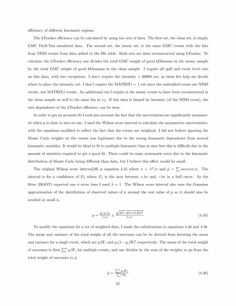
efficiency of different kinematic regions.

The kTracker efficiency can be calculated by using two sets of data. The first set, the clean set, is simply

GMC Drell-Yan simulated data. The second set, the messy set, is the same GMC events with the hits

from NIM3 events from data added to the Hit table. Both sets are then reconstructed using kTracker. To

calculate the kTracker efficiency one divides the total GMC weight of good kDimuons in the messy sample

by the total GMC weight of good kDimuons in the clean sample. I require all spill and event level cuts

on this data, with two exceptions. I don’t require the intensity < 60000 cut, as these fits help me decide

where to place the intensity cut. I don’t require the MATRIX1 = 1 cut since the embedded events are NIM3

events, not MATRIX1 events. An additional cut I require is the messy events to have been reconstructed in

the clean sample as well to the same bin in xT . If this data is binned by intensity (of the NIM3 event), the

rate dependence of the kTracker efficiency can be seen.

In order to get an accurate fit I took into account the fact that the uncertainties are significantly asymmet-

ric when p is close to zero or one. I used the Wilson score interval to calculate the asymmetric uncertainties,

with the equations modified to reflect the fact that the events are weighted. I did not believe ignoring the

Monte Carlo weights on the events was legitimate due to the strong kinematic dependence from several

kinematic variables. It would be ideal to fit to multiple kinematic bins at once but this is difficult due to the

amount of statistics required to get a good fit. There could be some systematic error due to the kinematic

distribution of Monte Carlo being different than data, but I believe this effect would be small.

The original Wilson score interval[49] is equation 4.45 where x = λ2/n and p =∑success/n. The

interval is for a confidence of Pλ where Pλ is the area between +λσ and −λσ in a bell curve. As the

fitter (ROOT) expected one σ error bars I used λ = 1. The Wilson score interval also uses the Gaussian

approximation of the distribution of observed values of p around the real value of p so it should also be

avoided at small n.

p =p+0.5x

1+x±√p(1−p)x+0.25x2

1+x(4.45)

To modify the equations for a set of weighted data, I made the substitutions in equations 4.46 and 4.56.

The mean and variance of the total weight of all the successes can be be derived from knowing the mean

and variance for a single event, which are piWi and pi(1− pi)W 2i respectively. The mean of the total weight

of successes is then∑ni piWi for multiple events, and one divides by the sum of the weights to go from the

total weight of successes to p.

p =∑n

i piWi∑ni Wi

(4.46)

87

To get 4.56 we need the variance so we can find a substitution that is analogous to the part of the original

derivation in equations 4.47, 4.48, and 4.49.

(p− p)2 = λ2σ2p (4.47)

(p− p)2 = λ2p(1− p)/n (4.48)

(p− p)2 = xp(1− p) (4.49)

Find the variance of the total weight of success.

σ2 =

n∑i

pi(1− pi)W 2i (4.50)

Get the variance of p.

σ2p =

∑ni pi(1−pi)W 2

i

(∑n

i Wi)2(4.51)

Assign εi as the difference between mean p and pi.

σ2p =

∑ni (p+εi)(1−p−εi)W 2

i

(∑n

i Wi)2(4.52)

σ2p = p(1− p)

∑ni W

2i

(∑n

i Wi)2+

∑ni εiW

2i

(∑n

i Wi)2−

∑ni 2pεiW

2i

(∑n

i Wi)2−

∑ni ε

2iW

2i

(∑n

i Wi)2(4.53)

Assume all the εi are insignificantly small.

σ2p ≈ p(1− p)

∑ni W

2i

(∑n

i Wi)2(4.54)

1n

=∑n

i W2i

(∑n

i Wi)2(4.55)

x = λ2∑n

i W2i

(∑n

i Wi)2(4.56)

The variance in this method is an approximation and so there will be some slight mistake in the length

88

of the error bars. However, the mean point is still placed correctly so I believe that overall this leads to good

fits.

I combine all the roadsets into one clean sample and one messy sample. Then I fit the efficiency of each

xT bin and each target as a function of chamber intensity, with a bin width of 5,000 and bins from 0 to

100,000 intensity. After trying several fit forms I found that exponential decay works the best. An example

of this fit can be found in figure 4.13.

Figure 4.14: Example of a fit of kTrackerEfficiency data to exponential decay.

The exponents for the fits for each xT bin show a clear xT dependence. Plotting these exponents as

a function of xT shows a linear relation between the fit exponent and xT . I fit a linear function to these

exponents to get the efficiency as a function of xT and intensity. The formula for the efficiency is in equation

4.57. Each individual dimuon is assigned an efficiency and is given a weight equal to 1/efficiency. The fitting

program also return a correlation matrix for the fit, which is necessary for proper uncertainty calculation,

especially in cases like these with strong off diagonal elements. The fit quantities can be found in table 4.3.3.

The fit for deuterium can be found in figure 4.14.

Efficiency = e−(p0+p1∗xT )∗intensity (4.57)

The fit values for the empty flask in table 4.3.3 were extrapolated from the LH2 and LD2 values based on

the nuclear interaction lengths of the targets because there are currently no empty flask GMC productions

with empty flask embedded random triggers. One can assume that the difference between the targets is a

function of how much of the beam interacts with the target. Using P0 Target as the kTracker efficiency p0

from table 4.3.3 for target T we can linearly extrapolate to come up with a formula for PE where no beam

89

target p0 p0 uncertainty p1 p1 uncertainty corr(p0, p1)

LH2 8.030e-6 5.170e-7 3.589e-5 1.914e-6 -0.929LD2 8.835e-6 5.926e-7 4.206e-5 2.206e-6 -0.926Empty 6.758e-6 1.628e-6 2.617e-5 6.039e-6 -0.927

Table 4.8: The fit parameters for the LD2 and LH2 targets and the empty flask. The empty flask fitparameters were extrapolated from the LH2 and LD2 parameters.

interacts with the target. p1 is calculated in the same manner.

Figure 4.15: Fitting the strength of the rate dependence as a function of xT .

P0 Empty = P0 LH2 − IFracLH2 ∗ ∆P0

∆IFrac(4.58)

P0 Empty = P0 LH2 − IFracLH2 ∗ P0 LD2−P0 LH2

IFracLD2−IFracLH2(4.59)

To find the affect of the uncertainty of the hydrogen fit on the cross section ratio, I calculate the cross

section ratio several times, once with the exponent at its normal value, and once each with p0 changed by

±1σ. The difference between the base cross section ratio and the +σ cross section ratio is KLH2 P0 Plus. I

calculate KLH2 P1 Plus in the same manner. The equation for calculating the overall upper uncertainty for

the hydrogen fits is equation 4.60. The lower uncertainties and the deuterium uncertainties are calculated

in the same manner.

σ =√K2LH2 P0 Plus +K2

LH2 P1 Plus + CorrLH2(p0, p1) ∗KLH2 P0 Plus ∗KLH2 P1 Plus (4.60)

90

It should be noted that both the messy and clean samples have 6% of the Monte Carlo hits removed (the

same hits). This was done to simulate chamber inefficiency, although the chamber inefficiency is not well

known. This could be related to the fact that some events that failed to reconstruct in the clean sample

were successfully reconstructed in the messy sample. Additionally, the residuals between the reconstructed

quantities and those of Monte Carlo truth were similar for events reconstructed in the clean sample and

events only reconstructed in the messy sample. It has been hypothesized that a messy hit near a removed

true hit can aid the reconstruction, therefore the chamber efficiency could have an effect on the strength

of the kTracker efficiency. A study that is a good idea but which has not been done yet is to redo the

kTracker efficiency studies at several different simulated chamber inefficiencies to study the correlation

between chamber efficiency and kTracker efficiency.

I considered the possibility that the true rate dependence of the kTracker efficiency could be on trigger

intensity instead of chamber intensity. If efficiency is graphed as a function of trigger intensity there is a

strong correlation with it. Trigger intensity and chamber intensity are strongly correlated so a dependence

on one can appear similar to a dependence on the other. To test how much of a dependence there was

on each type of intensity I graphed the efficiency of LD2 as a function of chamber intensity while cutting

all dimuons not between 20,000 and 30,000 trigger intensity. Then I graphed the efficiency as a function

of trigger intensity while cutting all dimuons not between 20,000 and 30,000 chamber intensity. Figure

4.15 where I fixed trigger intensity and let chamber intensity vary still shows a strong dependence, while

figure 4.16 where chamber intensity was fixed while trigger intensity was varied is flat. It is clear that the

dependence of kTracker efficiency is on chamber dependence.

Figure 4.16: The dependence of the kTracker efficiency on chamber intensity, with dependence on triggerintensity removed.

91

Figure 4.17: The dependence of the kTracker efficiency on trigger intensity, with dependence on chamberintensity removed.

4.3.4 Empty Flask Correction

The empty flask data has a strong rate dependence, with many more reconstructed dimuons per proton being

found at higher intensities. When the d/u analysis was being developed, a single fit was made to the rate

dependence for each target without breaking the rate dependence down into its components. Additionally,

an empty flask correction was made that had no rate dependence in it. Because of the strong but unknown

rate dependence of empty flask events, this led to the rate dependent part of the empty flask events being

corrected for twice, once in the empty target correction and once in the rate dependence correction. The shift

in the cross section ratio from this mistake was significant enough that the d/u extraction was inconsistent

with E866. Now the empty flask correction is a rate dependent correction. The lesson to be learned here is

that different corrections should not be assumed to be independent of each other. There was no reason to

expect rate dependence in the empty target correction, but we found it there anyway.

The point of the empty flask correction is to remove the influence of several sources of false positives of

dimuons originating from the target. If dimuons being generated from the dump or the upstream apparatus

are being reconstructed to the target region then they will also show up in data taken on an empty flask. If a

single muon from the dump and a single muon from upstream are being reconstructed together as a dimuon

from the target region, that too will show up in data taken on an empty flask. Since there is no target the

data will be lacking any true dimuons that originate from the target. Thus, the rate of empty flask dimuons

can be subtracted from the rate of liquid target dimuons to get the rate of true liquid target dimuons.

To correct for the empty flask events I calculated the ratio of empty flask dimuons per empty flask

92

Figure 4.18: The rate dependence of empty flask events. It is strongly rate dependent but also does not goto zero at zero intensity.

proton to liquid target dimuons per liquid target proton, binned in chamber intensity. In this calculation

the dimuons were given weights according to the kTracker efficiency fits. I then calculated the natural log

of these ratios and graphed them vs. chamber intensity. I made a linear fit and the parameters for each

liquid target can be found in table 4.9. The value of the fit at any intensity is the natural log of the chance

that a liquid target dimuon is actually from a non-target source. Each dimuon is given a weight according

to equation 4.61, where I is the intensity and K is the weight given to them from the kTracker efficiency

fits. p0 and p1 are the y-intercept and linear coefficient for the linear fit, respectively. An example of one of

these fits is in figure 4.18.

Target p0 p0 uncertainty p1 p1 uncertainty corr(p0, p1)

LH2 -2.323 8.835e-2 1.014e-5 2.805e-6 -0.8933LD2 -3.062 8.820e-2 1.251e-5 2.803e-6 -0.8933

Table 4.9: Table of parameters for empty flask corrections.

Weight = (1− ep0+p1∗I) ∗K (4.61)

To find the effect of the uncertainty of the empty flask fits on the cross section ratio, I calculate the

cross section ratio several times, once with the fit parameters at their normal values, once each with p0 for

both targets changed by ±1σ, and once each with p1 for both targets changed by ±1σ. Since most of the

uncertainty in the parameters came from the low empty flask statistics I changed the parameters for both

93

Figure 4.19: A fit of the natural log of the ratio of empty flask events to liquid target events, corrected forthe number of protons on each target.

targets at the same time instead of calculating individual uncertainties for each liquid target. The difference

between the base cross section ratio and the +σp0 cross section ratio is EP0 Plus. I calculate EP1 Plus in

the same manner. The equation for calculating the overall upper uncertainty is equation 4.62. The lower

uncertainties are calculated in the same manner.

σ =√E2P0 Plus + E2

P1 Plus + Corr(p0, p1) ∗ EP0 Plus ∗ EP1 Plus (4.62)

It is possible that the empty target correction should be slightly reduced to account for the attenuation

of the beam through the target that is not present with the empty flask in place. This would be needed if the

contribution was mostly dimuons from the dump. However, without knowing how many of the empty flask

constructed dimuons come from the dump, how many from upstream, and how many from a combination

of two independent muons from upstream or dump, it is not possible to properly tune the empty target

correction in such a way.

Like the kTracker efficiency correction, I considered the possibility of the fits having a stronger dependence

on trigger intensity. This seemed very likely since most of the empty flask dimuons are probably made up

of real tracks. Since hits from tracks from buckets outside the triggering bucket would not line up correctly

when kTracker attempts to reconstruct them, tracks from outside the triggering bucket would be much less

likely to contribute to empty flask false positives. Unlike with kTracker efficiency, making graphs for a small

range of trigger intensity and graphing vs chamber intensity was not viable due to the much lower statistics.

However, figure 4.19 is good evidence that there is almost no trigger intensity dependence in the empty flask

94

events.

Figure 4.20: The rate dependence of empty flask events when plotted against trigger intensity instead ofchamber intensity. It is relatively flat.

4.3.5 Remaining Rate Dependence

After applying both the kTracker efficiency and empty flask corrections there is still some rate dependence

with a positive slope. The origin of this rate dependence is not yet known. The rate dependence for the

deuterium target is shown in figure 4.20. Since I had trouble fitting both LH2 and LD2 targets to the same

shape and in general the fits were bad, I decided to fit a graph of the natural log of the ratio of LD2 and

LH2. I would assume that the rate dependence goes to zero at zero intensity and take the y-intercept of the

fit as the true value. The idea is to weight the LD2 dimuons based on the fit so that the natural log of the

ratio at any intensity value is equal to the natural log of the ratio at intensity equal to zero. I find it useful

to break the fit f(I) = ln(LD2LH2

(I)) down into an intercept p0 and a rate dependent part g(I).

ln(LD2LH2

(0)) = ln(LD2LH2

(I) ∗W (I)) (4.63)

p0 = ln(LD2LH2

(I)) + ln(W (I)) (4.64)

p0 = p0 + g(I) + ln(W (I)) (4.65)

95

Figure 4.21: The remaining rate dependence after the kTracker efficiency and the empty flask corrections.It is still not very flat.

W (I) = e−g(I) (4.66)

The final weight of an LD2 dimuon is the weight from equation 4.66 multiplied by the weights from

the kTracker efficiency and empty target corrections. LH2 dimuons just use the empty flask and kTracker

efficiency weights.

This method of weighting the dimuons makes the results very dependent on what the y-intercept turns

out to be. I tried a variety of fits and got reasonable results from multiple fits that had significantly different

y-intercepts. Figures 4.21 through 4.23 show the fits that I tried. I prefer the fit that is a quadratic fit

without a linear term because it has a balance between good χ2 and a small number of parameters, so I

used it as the main fit. However, since the shape of this fit wasn’t a clear winner, I used the other two fits

as well to generate systematic uncertainties related to this correction. Equation 4.67 gives the additional

weight added to deuterium dimuons to correct for the remaining rate dependence.

W (I) = e−3.988e−11∗I (4.67)

To find the effect of the remaining rate dependence fits on the cross section ratio, I calculate the cross

section ratio several times, once with the p1 fit parameter at its normal value, and once each with p1 for

changed by ±1σ. These give the upper and lower uncertainties from the fit parameter. I also calculate the

cross section ratio using the linear and quadratic fits. The difference between the linear fit and the nominal

fit is the upper uncertainty from the choice of fit shape and the difference between the quadratic fit and

96

Figure 4.22: The natural log of the ratio of LD2 to LH2 as a function of chamber intensity. It is fit with alinear fit.

Figure 4.23: The natural log of the ratio of LD2 to LH2 as a function of chamber intensity. It is fit with aquadratic fit.

97

Figure 4.24: The natural log of the ratio of LD2 to LH2 as a function of chamber intensity. It is fit with aquadratic fit that is missing the linear term.

the nominal fit is the lower systematic uncertainty from the choice of fit shape. Both upper uncertainties

are added in quadrature to get the upper uncertainty associated with the remaining rate dependence, and

similarly for the lower uncertainty.

I also considered the possibility of a stronger dependence on trigger intensity than on chamber intensity.

Looking at figure 4.24 it looks as though the dependence on trigger intensity is weaker. Because simply eye

balling it or choosing the graph with the strongest slope isn’t enough justification for such a decision, I made

two graphs. The first, figure 4.25, shows the dependence on trigger intensity after the points have been

weighted according to the fit from figure 4.23. The second, figure 4.26, shows the dependence on chamber

intensity after the points have been weighted according to the fit from figure 4.24. Both of the graphs are

relatively flat, so it is difficult to discern what the graphs truly depend on, so I went with the fit to chamber

intensity since it has a stronger correlation. This will be worth looking at again when the experiment has

more data and less statistical uncertainty.

I also checked for a dependence in these fits on xT . To check this, I divided the data up into an xT < 0.2

half and a xT > 0.2 half. I made graphs for each after weighting the points based on the fit from figure 4.23.

As can be seen in figures 4.27 and 4.28 both of these graphs seem reasonably flat after the correction, so

there is probably no xT dependence in this rate dependence correction. Again, this will be worth looking at

again when the experiment has more data and less statistical uncertainty.

98

Figure 4.25: The natural log of the ratio of LD2 to LH2 as a function of trigger intensity. It is fit with aquadratic fit that is missing the linear term. The dependence is not as strong as the chamber dependence.

Figure 4.26: The natural log of the ratio of LD2 to LH2 as a function of trigger intensity. The points havebeen weighted based on a fit to the trigger intensity. It seems flat within the uncertainties.

99

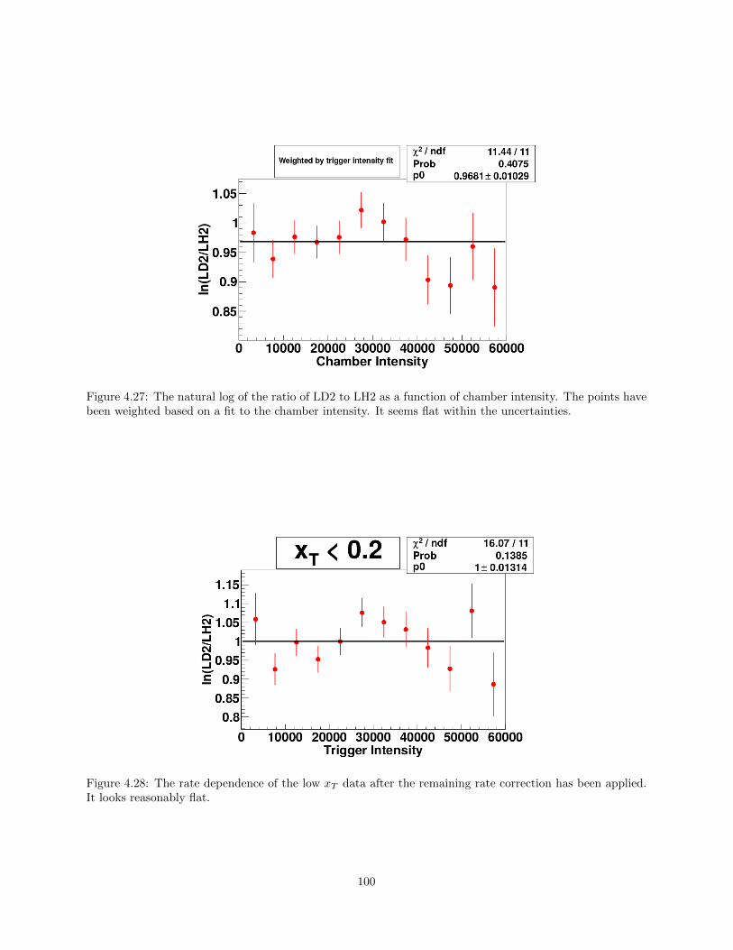
Figure 4.27: The natural log of the ratio of LD2 to LH2 as a function of chamber intensity. The points havebeen weighted based on a fit to the chamber intensity. It seems flat within the uncertainties.

Figure 4.28: The rate dependence of the low xT data after the remaining rate correction has been applied.It looks reasonably flat.

100

Figure 4.29: The rate dependence of the high xT data after the remaining rate correction has been applied.It looks reasonably flat.

4.4 Target Contamination

As mentioned earlier, the liquid deuterium target has a significant contamination from 1H. We have to

correct for the fact that some dimuons on the LD2 target come from Hydrogen atoms. Using Tx as the

target cross section, p as the proton-proton cross section, n as the proton-neutron cross section, LH2 and

LD2 as the cross sections between a proton and the pure material, a and c as the number of protons per

atom in LH2 and LD2 targets, and b and d as the number of neutrons per atom in the LH2 and LD2 targets,

respectively (which are the fractions of deuterium atoms in those targets):

TH = ap+ bn (4.68)

TD = cp+ dn (4.69)

Basic linear algebra results in:

LH2 = p =bTD−dTHbc−ad (4.70)

n =aTD−cTHad−bc (4.71)

101

LD2 = p+ n (4.72)

a and c are both one, since the number of protons in a hydrogen or deuterium atom are both one. Our

LH2 target is also pure to several digits of precision, so we can set b to zero. d ranges between 0.9 and 1,

and closer to one the less contamination there is. I will refer to it as Pu for purity for the rest of the thesis.

LH2 = p = TH (4.73)

n =TD−THPu

(4.74)

LD2 = TH +TD−THPu

(4.75)

The amount of contamination in our target (for most of our data) has an uncertainty. To calculate the

uncertainty in the cross section ratio as a result of this I calculate the cross section three times, once with the

contamination at the base value and once each with the contamination raised or lowered by the uncertainty.

The difference between the base cross section and the cross section at the limits of the contamination is a

systematic uncertainty in the cross section ratio. These contamination uncertainties are very asymmetric

and are found in table 2.3.

4.5 Logarithm of the Ratio

In previous experiments, what has been published has been d/u (or u/d) and cross section ratios. However,

I believe the best way to present the data is ln(d/u) and ln(σpd/2σpp).

In the E866 experiment, there were multiple data sets that were analysed separately before combining

their σpd/2σpp results into a single result. Each data set i had a weight Wi equal to 1/σ2i , where σi is the

statistical uncertainty of the ratio in data set i. Using ri as the ratio of data set i and R as the final ratio,

equation 4.76 was used to calculate R for E866[50][30].

R =

∑i riWi∑iWi

±√

1/∑

iWi (4.76)

I will use a simple example to show why equation 4.76 is not a good choice. In a hypothetical experiment

measuring the ratio RX/Y of events of type X and events of type Y there are two data sets, A and B, where

102

all conditions are the same. The split into A and B is arbitrary and they could have been one combined

data set, which we’ll call C. The statistics for each data set are listed in table 4.10.

Data Set X Y

A 4 2B 2 4

C 6 6

Table 4.10: A very simple example of a data set C, arbitrarily split into data sets A and B. Both X and Yfollow Poisson distributions.

Now, for a single data set, the statistical uncertainty in X/Y to first order should be equation 4.77. E866

did not use higher order uncertainties[51].

σR =

√(σX

1Y

)2 + (σYXY 2 )2 (4.77)

σR =X

Y

√(σXX

)2 + (σYY

)2 (4.78)

Which leads us to table 4.11.

Data Set X Y R σX σY σR W

A 4 2 2 2√

2√

3 13

B 2 4 0.5√

2 2√

34

163

A merge B 0.59 0.42 5.67

C 6 6 1√

6√

6 0.58 3

Table 4.11: Table 4.10 with more fields.

Using equation 4.76 to combine data sets A and B, we get a result of RX/Y = 1017 ±

√3/17 = 0.59± 0.42,

which is clearly incorrect. The result for C is R = 1 ± 0.58. The data set with the lower ratio has been

given too much of a weight, and the data set with the higher ratio has been given too little of a weight,

by a large margin. It is clear that the X/Y term in front of the square root in equation 4.78 is the culprit,

suggesting that when the values of the data sets being merged are farther apart the error will be large.

Instead of combining the ratios from different data sets, we could combine a different function of both X

and Y. Ideally, we’d want something symmetric with respect to X and Y to avoid the above problem. An

ideal function would be equal to zero at X = Y and have the property f(X, Y) = -f(Y, X). ln(X/Y) is such

a function.

103

ln(R) = ln(X)− ln(Y ) (4.79)

σln(R) =√

(σXX

)2 + (σYY

)2 (4.80)

The weights are now no longer biased towards high Y, but give even weight to X statistics and Y statistics.

Using ln(R), its uncertainty, and combining the data sets using equation 4.76 gives a much different result,

found in table 4.12. This is the same as calculating a weighted geometric mean, with weights based off of

equation 4.80.

Data Set X Y R ln(R) σX σY σln(R) W

A 4 2 2 0.693 2√

2√

32

43

B 2 4 0.5 -0.693√

2 2√

32

43

A merge B 1 0 0.61 2.67

C 6 6 1 0√

6√

6 0.58 3

Table 4.12: Like table 4.11, but for a logarithmic study.

Using equation 4.76 to combine data sets A and B, we get a result of ln(RX/Y ) = 0±0.61, which is more

sane. The value of R is 1 and the 1 σ confidence interval for R is 0.54 to 1.84. The confidence interval for

R from C is 0.56 to 1.78, so this isn’t perfect, but it is quite an improvement. The confidence interval for

R from C using the old method is 0.42 to 1.58. When using the natural log method the lower uncertainty

is less while the upper uncertainty is greater. It should also be noted that in more complicated examples

where ln(R) 6= 0 that the log method does not find the correct average to 100% accuracy, although it is a

lot closer that the old method. This can be improved by calculating uncertainties and expected values with

higher order terms.

To convert older data, R can be turned into ln(R) easily enough. By comparing equations 4.78 and 4.80,

we can get equation 4.81.

σln(R) =Y

XσR (4.81)

Using this on the last data point of E866 for the high mass setting yields table 4.13. Note that the

binning is different than that of the combined results from all mass settings that is the most well known

E866 data. The difference between the two methods is not very large for the cross section ratio, but d/u

changes by over a factor of two for changes in σpd/2σpp and over a factor of three at higher x in E866,

104

magnifying the effects of this error for d/u. I have not been able to get my hands on the combined mass

settings results broken down into data sets for E866, so I have not been able to correct those results like

this. The correction for those points could be smaller or much larger than this correction. While I will plot

E866 data later, keep in mind that the high uncertainty points at high x are likely lower than they should

be.

Data Set Ratio Stat Weight Ln Ln Stat Ln Weight

7 0.843 0.277 13.033 -0.171 0.329 9.2398 0.873 0.179 31.21 -0.136 0.202 24.50711 1.251 0.448 4.982 0.224 0.358 7.803

E866 merge 0.903 0.143 -0.102 0.129ln merge 0.927 0.144 -0.076 0.155

Table 4.13: Corrected cross section ratio values for the E866 high mass setting. Ratio and Ratio Stat arethe traditional cross section ratio and their uncertainties. Log is ln(σpd/2σpp). Log Stat is the uncertaintyon ln(σpd/2σpp). Ln Weight is the weight used when combining separate data sets using the log method.

In this analysis the different data sets are combined before calculating the cross section ratio, so I do

not have to worry about the data points in SeaQuest being incorrect because of this effect. The comparison

of SeaQuest data to E866 data is inevitable however and the errors in combining data sets sheds light

on potential apparent discrepancies between SeaQuest and E866 data points at high x. However, another

reason to use ln(R) is sensible confidence intervals, and this does apply to SeaQuest. A large uncertainty

combined with a low point can put some of the confidence interval for R below zero. The last d/u point in

E866[52] is 0.346 ± 0.396, which puts some of the interval below zero, a region which is physically impossible.

With ln(R), the confidence interval is restricted to physically possible values. In regular ratio plots, Y >

X is crammed between 0 and 1 while X > Y stretches from 1 to infinity, and this is reflected in the upper

uncertainties being shorter than they should be and the lower uncertainties being larger than they should

be. The choice of which value goes in the numerator and which in the denominator is arbitrary. The

presentation of the data should be balanced between the X > Y region and the Y > X region. In a ln plot

X > Y covers the positive half and Y > X covers the negative half and there is no stretching or contraction

of the uncertainty interval.

4.6 Cross Section Ratio Calculation

The yield of Drell-Yan events, based on the cross section, can be found in equation 4.82. This can be

rearranged to calculate the cross section based off the yield.

105

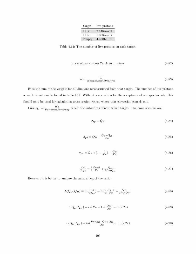
target live protons

LH2 2.1402e+17LD2 1.0632e+17Empty 4.3201e+16

Table 4.14: The number of live protons on each target.

σ ∗ protons ∗ atomsPerArea = Y ield (4.82)

σ = Wprotons∗atomsPerArea (4.83)

W is the sum of the weights for all dimuons reconstructed from that target. The number of live protons

on each target can be found in table 4.14. Without a correction for the acceptance of our spectrometer this

should only be used for calculating cross section ratios, where that correction cancels out.

I use QT =WT

PT ∗atomsPerAreaTwhere the subscripts denote which target. The cross sections are:

σpp = QH (4.84)

σpd = QH +QD−QH

Pu(4.85)

σpd = QH ∗ (1− 1Pu

) +QD

Pu(4.86)

σpd2σpp

= 12Pu−1Pu

+QD

2Pu∗QH(4.87)

However, it is better to analyse the natural log of the ratio.

L(QD, QH) ≡ ln(σpd2σpp

) = ln(12Pu−1Pu

+QD

2Pu∗QH) (4.88)

L(QD, QH) = ln(Pu− 1 +QD

QH)− ln(2Pu) (4.89)

L(QD, QH) = ln(Pu∗QH−QH+QD

QH)− ln(2Pu) (4.90)

106

L(QD, QH) = ln(QD − (1− Pu)QH)− ln(QH)− ln(2Pu) (4.91)

To analyse the statistical uncertainty on the cross section the statistical uncertainties on QH and QD are

needed. There are two sources of uncertainty, the total number of events on LH2 or LD2 and the average

weight of those events. Using W as the average weight, Y as the total number of events from that target,

and W as the total weight, the equation for the uncertainty on the total weight of events from a target is in

equation 4.92. The uncertainty on the average weight is the standard deviation of the mean of the weights.

The uncertainty on the yield is√YT since it is a Poisson distribution.

σ2WT

= σ2YTW 2T + σ2

WTY 2T (4.92)

σ2QT

=σ2WT

(PT ∗atomsPerAreaT )2(4.93)

Several partial derivatives are also needed for calculating the expected value to second order and the

uncertainty to first order. I believe that with large uncertainties on the points at high x that a first order

analysis of the expected value is difficult to justify, even with the log method reducing the need for higher

order terms.

δLδQD

= 1Pu∗QH−QH+QD

(4.94)

δLδQH

= ( Pu−1d∗QH−QH+QD

− 1QH

) (4.95)

δ2Lδ2QD

= −1(Pu∗QH−QH+QD)2

(4.96)

δ2Lδ2QH

=−(Pu−1)2

(Pu∗QH−QH+QD)2+ 1

Q2H

(4.97)

In the following equations I will use σ2 to indicate the variance, it will not indicate cross sections.

E(variable) is the notation for the expected value of that variable. The expected value will use all the terms

from a second order Taylor expansion[53], but the uncertainty will just be first order. When I later report

the cross section ratios in the results section, I will report E(ln( D2H

)), not ln(E(D)2E(H)

).

107

E(L(QD, QH)) = L(E(QD), E(QH)) + 12δ2Lδ2QD

σ2QD

+ 12δ2Lδ2QH

σ2QH

(4.98)

σ2L = ( δL

δQD)2σ2

QD+ ( δL

δQH)2σ2

QH(4.99)

In order to justify combining all the data before calculating the cross section ratios, I checked the

kinematic distributions for each of the large roadsets to make sure they matched. Roadsets 59 and 70 had

too few statistics to check in this way. I graphed xT , xB , and pT for all the roadsets with their areas

normalized to be equal in figures 4.29 through 4.33. Since they are so similar, this justifies merging the cross

section ratio results together. This is the best approach if it can be justified as it keeps the uncertainties as

small as possible. The smaller the uncertainties, the more accurate the uncertainty propagation. This also

allows the inclusion of data sets where the uncertainties are too large to do a proper d/u extraction.

Figure 4.30: Plot of the XT distribution for all three roadsets. The areas under the curves have beennormalized to the same value.

The collaboration decided that statistical uncertainties would be those uncertainties that are uncorrelated

between bins and systematic uncertainties would be those uncertainties that are correlated between bins.

The basis of this decision is how groups like CTEQ will fit our data. Each point of our data will be allowed to

move up and down a distance based on its statistical uncertainty, while the collection of our data points as a

whole will be allowed to together move a distance based on the systematic uncertainties. The sources for the

statistical uncertainty comes from the statistical uncertainties in the LH2 total weight and LD2 total weight.

108

Figure 4.31: Plot of the XB distribution for all three roadsets. The areas under the curves have beennormalized to the same value.

Figure 4.32: Plot of the XF distribution for all three roadsets. The areas under the curves have beennormalized to the same value.

109

Figure 4.33: Plot of the mass distribution for all three roadsets. The areas under the curves have beennormalized to the same value.

Figure 4.34: Plot of the PT distribution for all three roadsets. The areas under the curves have beennormalized to the same value.

110

These sources are added in quadrature. The sources of systematic uncertainty are the kTracker efficiency

fits, the empty flask fits, the remaining rate dependence fits, the uncertainty from the target contamination,

and the uncertainty from nuclear effects in deuterium. All of the systematic uncertainties are added in

quadrature.

There is no correction calculated for the contamination of the results from J/Ψ and Ψ′ dimuons. In a

J/Ψ Monte Carlo reconstructed by kTracker there were no reconstructed dimuons above the mass threshold

that passed validity and target cuts. In a Ψ′ Monte Carlo reconstructed by kTracker, out of all the valid

reconstructed dimuons passing the target cut, 0.31% were above the mass threshold. Some thought is due

to how much of a systematic error to place on this, but it will be very small.

There is no correction calculated for the contamination of the results from combinatorial background.

As combinatorial background is proportional to intensity2 while dimuons are proportional to intensity, the

combinatorial background as a fraction of our data should go to zero in the limit that intensity goes to zero.

This means it is a rate dependent contamination, and the remaining rate dependence has been corrected

for and uncertainties associated with it have been assigned. Once the experiment has taken enough like

sign coincidence data then the combinatorial background can be accurately calculated and assigned its own

correction. Much care should be taken to estimate how much it overlaps with the empty target and remaining

rate dependence corrections.

There is no correction calculated for chamber inefficiency. As mentioned in the kTracker efficiency section,

even a non rate dependent chamber inefficiency might affect the rate dependence, and the two effects need to

be untangled with more study. However, since we don’t know the chamber efficiencies well, then a correction

for this can not be made.

4.7 d/u Extraction

Once the log of the ratio of LD2/LH2 cross sections is obtained from data, which I will call Ld, it is time to

calculate d/u. First, an initial estimate of d/u is set, although this initial value is not important. Then, for

each dimuon in the yield of LH2 and LD2, an estimate of the log of the cross section ratio for that dimuon’s

mass, xB , and xT is calculated with the initial value of d/u. The mean value of all of the predictions is

taken as the prediction of the log of the cross section ratio, which I will call Lp. The difference Ld − Lp is

then used to modify the estimate of d/u. This procedure is then repeated until Ld = Lp within 1e-4.

In all calculations the d + u distribution and all quark distributions other than d and u are taken from

a PDF set. d/u inside the analysis range for both beam and target quarks is taken from the current

111

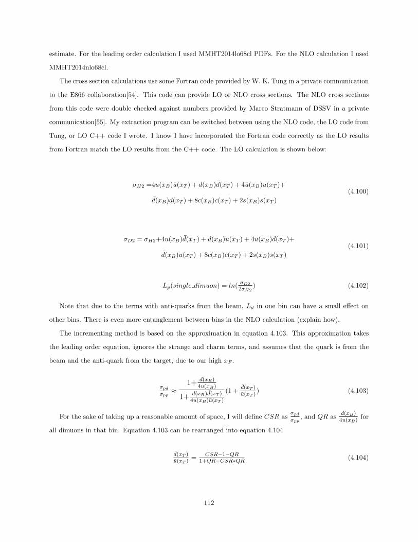
estimate. For the leading order calculation I used MMHT2014lo68cl PDFs. For the NLO calculation I used

MMHT2014nlo68cl.

The cross section calculations use some Fortran code provided by W. K. Tung in a private communication

to the E866 collaboration[54]. This code can provide LO or NLO cross sections. The NLO cross sections

from this code were double checked against numbers provided by Marco Stratmann of DSSV in a private

communication[55]. My extraction program can be switched between using the NLO code, the LO code from

Tung, or LO C++ code I wrote. I know I have incorporated the Fortran code correctly as the LO results

from Fortran match the LO results from the C++ code. The LO calculation is shown below:

σH2 =4u(xB)u(xT ) + d(xB)d(xT ) + 4u(xB)u(xT )+

d(xB)d(xT ) + 8c(xB)c(xT ) + 2s(xB)s(xT )

(4.100)

σD2 = σH2+4u(xB)d(xT ) + d(xB)u(xT ) + 4u(xB)d(xT )+

d(xB)u(xT ) + 8c(xB)c(xT ) + 2s(xB)s(xT )

(4.101)

Lp(single dimuon) = ln(σD2

2σH2) (4.102)

Note that due to the terms with anti-quarks from the beam, Ld in one bin can have a small effect on

other bins. There is even more entanglement between bins in the NLO calculation (explain how).

The incrementing method is based on the approximation in equation 4.103. This approximation takes

the leading order equation, ignores the strange and charm terms, and assumes that the quark is from the

beam and the anti-quark from the target, due to our high xF .

σpdσpp≈

1+ d(xB)4u(xB)

1+ d(xB)d(xT )4u(xB)u(xT )

(1 +d(xT )u(xT )

) (4.103)

For the sake of taking up a reasonable amount of space, I will define CSR asσpdσpp

, and QR asd(xB)

4u(xB)for

all dimuons in that bin. Equation 4.103 can be rearranged into equation 4.104

d(xT )u(xT )

=CSR−1−QR

1+QR−CSR∗QR (4.104)

112

ln(d(xT )u(xT )

) = ln(CSR− 1−QR)− ln(1 +QR− CSR ∗QR) (4.105)

Taking a derivative leads us to equations 4.106 and 4.107.

δln(d(xT )u(xT )

)

δCSR= 1

CSR−1−QR +QR

1+QR−CSR∗QR (4.106)

∆ln(d(xT )u(xT )

) = ∆CSR( 1CSR−1−QR +

QR1+QR−CSR∗QR ) (4.107)

QR is calculated for every dimuon and log averaged. ∆CSR is the difference between Ld and Lp. CSR

is the average of Ld and Lp. Equation 4.107 is good but not perfect, and NLO computations can take a

long time, so I modified it to equation 4.108 where i is the iteration it is on and F1 = 1. This decreases the

magnitude of the iteration if it overshoots and increases the magnitude when it falls short. This method

converges in about 6 iterations, which is very useful when calculating NLO results.

∆ln(d(xT )u(xT )

) = ∆CSR( 1CSR−1−QR +

QR1+QR−CSR∗QR )Fi (4.108)

Fi = (∆CSRi−1

∆CSRi−1−∆CSRi) ∗ Fi−1 (4.109)

To confirm that the results do not depend upon the initial estimate, I ran the program with an initial

estimate of d/u = 0.5 for all bins and again for an initial estimate of d/u = 2.0 for all bins. The results were

identical.

Once d/u is calculated, the uncertainties are calculated. This requires running the extraction part of

the program 2n times more, where n is the number of bins. For the first n times, one bin of Ld is adjusted

upwards by an amount equal to its statistical uncertainty, while all other bins of Ld stay the same. The last

n times are similar, except the bin of Ld is adjusted downwards. The results of each of the 2n extractions

are compared to the original extraction of d/u, and the differences are taken as uncertainties. The resulting

uncertainties from increasing Ld are then added in quadrature to get the upper statistical uncertainties

for d/u. Similarly for the uncertainties from decreasing Ld and the lower statistical uncertainties. It is

important to note that changing Ld in one bin can affect the d/u results in other bins by a small amount.

In each bin I have calculated d/u with three different Ld values, which I will call L−, L0, and L+. I

will call the resulting ln(d/u) results y−, y0, and y+. If we take (L−, y−), (L0, y0), and (L+, y+) to be three

113

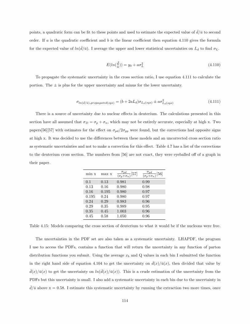
points, a quadratic form can be fit to these points and used to estimate the expected value of d/u to second

order. If a is the quadratic coefficient and b is the linear coefficient then equation 4.110 gives the formula

for the expected value of ln(d/u). I average the upper and lower statistical uncertainties on Ld to find σL.

E(ln( du

)) = y0 + aσ2L (4.110)

To propagate the systematic uncertainty in the cross section ratio, I use equation 4.111 to calculate the

portion. The ± is plus for the upper uncertainty and minus for the lower uncertainty.

σln(d/u) propagated(sys) = (b+ 2aLd)σLd(sys) ± aσ2Ld(sys) (4.111)

There is a source of uncertainty due to nuclear effects in deuterium. The calculations presented in this

section have all assumed that σD = σp + σn, which may not be entirely accurate, especially at high x. Two

papers[56][57] with estimates for the effect on σpd/2σpp were found, but the corrections had opposite signs

at high x. It was decided to use the differences between these models and an uncorrected cross section ratio

as systematic uncertainties and not to make a correction for this effect. Table 4.7 has a list of the corrections

to the deuterium cross section. The numbers from [56] are not exact, they were eyeballed off of a graph in

their paper.

min x max xσpd

(σp+σn)[57]

σpd(σp+σn)

[56]

0.1 0.13 0.981 0.990.13 0.16 0.980 0.980.16 0.195 0.980 0.970.195 0.24 0.980 0.970.24 0.29 0.983 0.960.29 0.35 0.989 0.950.35 0.45 1.003 0.960.45 0.58 1.050 0.96

Table 4.15: Models comparing the cross section of deuterium to what it would be if the nucleons were free.

The uncertainties in the PDF set are also taken as a systematic uncertainty. LHAPDF, the program

I use to access the PDFs, contains a function that will return the uncertainty in any function of parton

distribution functions you submit. Using the average xb and Q values in each bin I submitted the function

in the right hand side of equation 4.104 to get the uncertainty on d(x)/u(x), then divided that value by

d(x)/u(x) to get the uncertainty on ln(d(x)/u(x)). This is a crude estimation of the uncertainty from the

PDFs but this uncertainty is small. I also add a systematic uncertainty in each bin due to the uncertainty in

d/u above x = 0.58. I estimate this systematic uncertainty by running the extraction two more times, once

114

with d/u = 1.0 and once with it equal to the log average of the last two points. I also estimate an additional

systematic uncertainty associated with my choice of PDF set by running the extraction three more times

using the PDF sets CT14nlo, and abm11 5n as nlo. All of the systematic uncertainties have upper and lower

uncertainties estimated separately. All of the systematic uncertainties are added in quadrature.

115

Chapter 5

Results

The two main goals of this entire analysis are the estimation of the natural log of the cross section ratio,

ln(σpd2σpp

) and the estimation of the natural log of the ratio of sea antiquarks, ln( du

), both as a function of

x. The uncertainties on these values are also an essential part of the result. ln( du

) is the more fundamental

physics result of the two, and is the more important result that way. However, future experimenters and

theorists will be taking ln(d/u) from PDFs generated by groups such as CTEQ who fit the data from dozens

of different experiments instead of directly using the SeaQuest results. Undoubtedly SeaQuest will have an

important influence on these fits but groups such as CTEQ will be asking for our cross section ratio data,

so in one sense the cross section ratio is the main result of our experiment.

5.1 Cross Section Ratio

Not just our results are important in the use of our data by fitting groups, but the kinematics of those

results. The average kinematics of events in each bin of xT for the LH2 target is in table 5.1 and for the

LD2 target is in table 5.2. The total weights of the LH2 dimuons in each bin at each step of the analysis

are shown in table 5.3 and the weights of the LD2 dimuons are in table 5.4. ln(2σpd2σpp

) and its uncertainties

for each bin in xT is shown in table 5.5. A breakdown of the various uncertainties are provided in tables 5.6

and 5.7. A graph of the results is shown in figure 5.1.

xT range 〈xT 〉 〈xB〉⟨Q2⟩〈pT 〉

0.1-0.13 0.1199 0.7415 19.12 0.69930.13-0.16 0.146 0.6465 20.41 0.75230.16-0.195 0.1766 0.5894 22.63 0.78550.195-0.24 0.2148 0.565 26.52 0.83170.24-0.29 0.2626 0.5485 31.65 0.85710.29-0.35 0.3153 0.5383 37.4 0.90450.35-0.45 0.3852 0.5155 44.15 0.82840.45-0.58 0.4925 0.5143 56.34 0.911

Table 5.1: This table lists the average kinematics for reconstructed dimuons from the LH2 target. Thedimuons were weighted with the rate dependence weights.

116

xT range 〈xT 〉 〈xB〉⟨Q2⟩〈pT 〉

0.1-0.13 0.12 0.7468 19.24 0.71380.13-0.16 0.146 0.6484 20.48 0.74630.16-0.195 0.1768 0.5903 22.7 0.77880.195-0.24 0.2151 0.5655 26.66 0.79760.24-0.29 0.2624 0.5533 31.96 0.82980.29-0.35 0.3155 0.5382 37.51 0.8670.35-0.45 0.3863 0.5293 45.39 0.87630.45-0.58 0.4915 0.5126 56.2 0.8043

Table 5.2: This table lists the average kinematics for reconstructed dimuons from the LD2 target. Thedimuons were weighted with the rate dependence weights.

xT range raw yield kTracker efficiency correction empty flask correction0.1-0.13 1417 1991 17420.13-0.16 3892 5583 48880.16-0.195 4676 6854 60050.195-0.24 3722 5628 4320.24-0.29 1940 3082 26990.29-0.35 974 1610 14110.35-0.45 373 656.7 5750.45-0.58 67 134.2 117.4

Table 5.3: This table lists how many dimuons were reconstructed from the LH2 target for each bin, and thetotal weight of all the dimuons at each step.

Figure 5.1: A graph of ln(σpd2σpp

) as a function of xT .

117

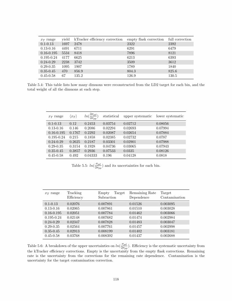
xT range yield kTracker efficiency correction empty flask correction full correction0.1-0.13 1697 2478 2322 23920.13-0.16 4491 6711 6291 64790.16-0.195 5534 8418 7896 81210.195-0.24 4177 6625 6213 63930.24-0.29 2238 3742 3509 36120.29-0.35 1095 1907 1789 18400.35-0.45 470 856.9 804.3 825.60.45-0.58 67 135.2 126.9 130.5

Table 5.4: This table lists how many dimuons were reconstructed from the LD2 target for each bin, and thetotal weight of all the dimuons at each step.

xT range 〈xT 〉 ln(2σpd2σpp

) statistical upper systematic lower systematic

0.1-0.13 0.12 0.2453 0.03754 0.02712 0.080560.13-0.16 0.146 0.2086 0.02294 0.02693 0.079940.16-0.195 0.1767 0.2292 0.02087 0.02654 0.078840.195-0.24 0.215 0.1858 0.02385 0.02732 0.07870.24-0.29 0.2625 0.2187 0.03301 0.02901 0.079880.29-0.35 0.3154 0.1928 0.04736 0.03065 0.079430.35-0.45 0.3857 0.2936 0.07533 0.0335 0.081260.45-0.58 0.492 0.04333 0.196 0.04128 0.0818

Table 5.5: ln(σpd2σpp

) and its uncertainties for each bin.

xT range TrackingEfficiency

Empty TargetSubraction

Remaining RateDependence

TargetContamination

0.1-0.13 0.02076 0.007891 0.01526 0.0030950.13-0.16 0.02065 0.007861 0.01510 0.0030280.16-0.195 0.02051 0.007784 0.01462 0.0030660.195-0.24 0.02148 0.007682 0.01474 0.0029840.24-0.29 0.02347 0.007828 0.01483 0.0030470.29-0.35 0.02564 0.007761 0.01457 0.0029980.35-0.45 0.02913 0.008199 0.01402 0.0031810.45-0.58 0.03768 0.008392 0.01437 0.002688

Table 5.6: A breakdown of the upper uncertainties on ln(σpd2σpp

). Efficiency is the systematic uncertainty from

the kTracker efficiency corrections. Empty is the uncertainty from the empty flask corrections. Remainingrate is the uncertainty from the corrections for the remaining rate dependence. Contamination is theuncertainty for the target contamination correction.

118

xT range TrackingEfficiency

Empty TargetSubraction

Remaining RateDependence

TargetContamination

0.1-0.13 0.02077 0.006994 0.07446 0.021610.13-0.16 0.02065 0.006968 0.07395 0.021130.16-0.195 0.02052 0.006913 0.07272 0.02140.195-0.24 0.02149 0.006827 0.07247 0.020820.24-0.29 0.02348 0.006943 0.07300 0.021260.29-0.35 0.02566 0.006894 0.07187 0.020920.35-0.45 0.02913 0.007236 0.07217 0.022210.45-0.58 0.03774 0.00743 0.06972 0.01873

Table 5.7: A breakdown of the lower uncertainties on ln(σpd2σpp

). The fields are the same as in table 5.6.

119

5.2 d/u

ln( du

) and its uncertainties can be found in table 5.8. A breakdown of the lower and upper uncertainties

into its parts can be found in tables 5.9 and 5.10. A graph of the results along with the results from E866

and NA51 can be found in figure 5.2.

x range 〈x〉 ln( du ) statistical + statistical - systematic + systematic -

0.1-0.13 0.12 0.4248 0.04545 0.04664 0.04425 0.15630.13-0.16 0.146 0.3955 0.0319 0.03361 0.04747 0.17210.16-0.195 0.1767 0.4356 0.03095 0.03137 0.06043 0.1670.195-0.24 0.215 0.3903 0.04211 0.03977 0.07345 0.17090.24-0.29 0.2625 0.4574 0.05549 0.05637 0.09165 0.17750.29-0.35 0.3154 0.4563 0.08609 0.08755 0.1202 0.17990.35-0.45 0.3857 0.6998 0.1396 0.1438 0.1496 0.16940.45-0.58 0.492 0.3013 0.446 0.5597 0.1327 0.2718

Table 5.8: ln( du

) and its uncertainties, binned in x.

x Range σpd/2σpp PDFUncertainty

d/uvery high x

PDF Choice DeuteriumNuclearEffects

0.1-0.13 0.03296 0.01824 4.318e-05 0.008149 0.021740.13-0.16 0.03727 0.006992 7.131e-05 0.01341 0.025220.16-0.195 0.03928 0.006418 0.0001408 0.01982 0.040930.195-0.24 0.04844 0.005004 0.0001028 0.02904 0.046690.24-0.29 0.0488 0.00575 0.0001378 0.04724 0.061260.29-0.35 0.05588 0.00498 0.0002164 0.06928 0.080570.35-0.45 0.06259 0.007403 0.000508 0.1139 0.073640.45-0.58 0.1034 0.001116 0.0006944 0.03736 0.0743

Table 5.9: The breakdown of upper systematic uncertainties on ln( du

). Propagated is the systematic un-certainty propagated from the cross section ratio. PDF uncertainty is the uncertainty within the PDF set.PDF high x is the uncertainty from the unknown value of ln(d/u) outside of our measuring range. PDFgroup is the systematic uncertainty from the choice of PDF set, i.e. we chose MMHT2014 instead of CT14.Nuclear correction is the systematic uncertainty from nuclear effects in deuterium.

The SeaQuest data shows no sign of dropping off at higher x like the E866 does, and the statistical

significance is strong up to the end of the E866 data. The data clearly shows that d does not drop below

u, removing a feature from the data that models had great difficulty in adjusting to. Our data is consistent

with E866 except for a couple of points in their high x region where their high uncertainties combined with

their error in merging the results of multiple data sets together has likely offset their data to lower than it

should be. Our data indicates that d(x)/u(x) flattens out at higher x, but with the high uncertainties it

is not possible to conclude whether it continues to slowly increase, flatten out asymptotically, or turn back

120

x Range σpd/2σpp PDFUncertainty

d/uvery high x

PDF Choice DeuteriumNuclearEffects

0.1-0.13 0.1015 0.02129 0.0004413 0.1169 00.13-0.16 0.1245 0.008956 0.0008264 0.1184 00.16-0.195 0.1207 0.006784 0.0007852 0.1152 00.195-0.24 0.1224 0.005051 0.0008979 0.1192 00.24-0.29 0.1379 0.005786 0.001241 0.1116 00.29-0.35 0.1477 0.005012 0.001977 0.1025 00.35-0.45 0.1553 0.00743 0.004794 0.06692 0.005570.45-0.58 0.2198 0.001123 0.008525 0.1273 0.09649

Table 5.10: The breakdown of lower systematic uncertainties on ln( du

). The fields are the same as in table5.9.

Figure 5.2: A graph of ln( du

) as a function of x.

121

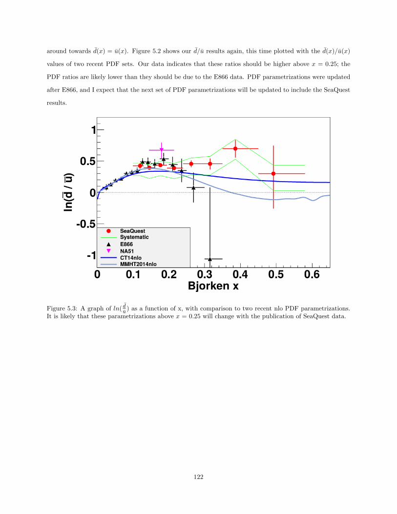
around towards d(x) = u(x). Figure 5.2 shows our d/u results again, this time plotted with the d(x)/u(x)

values of two recent PDF sets. Our data indicates that these ratios should be higher above x = 0.25; the

PDF ratios are likely lower than they should be due to the E866 data. PDF parametrizations were updated

after E866, and I expect that the next set of PDF parametrizations will be updated to include the SeaQuest

results.

Figure 5.3: A graph of ln( du

) as a function of x, with comparison to two recent nlo PDF parametrizations.It is likely that these parametrizations above x = 0.25 will change with the publication of SeaQuest data.

122

Chapter 6

Conclusions

The several main points to take away from this analysis are:

• d(x)/u(x) has been measured at SeaQuest at x between values of 0.1 and 0.58.

• This result is consistent with past experiments with the exception of a couple of high x data points

from E866, but this inconsistency has an explanation.

• The results overturn the E866 result that d < u at x past 0.3. This result is good news for the many

models attempting to accurately describe the mechanism behind the flavor asymmetric sea, as the

feature of d/u < 1 was difficult to incorporate into these models.

• This measurement shows that current d(x)/u(x) ratios in PDFs are too low at x past 0.25.

• It is worth considering exactly how to estimate x from measured quantities for Drell-Yan events as the

partons tend to have high pT that makes all known approximations less accurate.

• Uncertainties in the hydrogen contamination of the deuterium target for the earlier data lead to a large

contribution to the systematic error.

• The rate correction due to SeaQuest’s unstable beam is very complicated. A detailed attempt at a

correction was attempted in this thesis, and despite the large improvements to our data I think the

rate correction could possibly be improved with a better background subtraction method.

• Care needs to be taken to merge data sets when studying ratios of measured quantities to avoid an

error that systematically reduces the value of the ratio.

• While a simple d(x)/u(x) presentation of results is more intuitive, a less mathematically misleading

presentation of this ratio is ln(d(x)/u(x)).

• This thesis has not analysed all of the data taken. There is a lot of data from run 5 that has an extra

wire chamber installed to measure higher x events. The spectrometer had changed enough that I did

123

not consider this new data stable enough for this thesis, but there is every reason to think that it will

be analysed in a future publication. Another advantage of any newer data is the pure deuterium target

that will avoid the large systematic uncertainties associated with target contamination.

124

References

[1] M. Gell-Mann. A schematic model of baryons and mesons. Physics Letters, 8:214–215, 1964.

[2] G. Zweig. An su3 model for strong interaction symmetry and its breaking. 1964.

[3] O. W. Greenberg. Spin and unitary-spin independence in a paraquark model of baryons and mesons.Physical Review Letters, 13:598–602, 1964.

[4] Michael E. Peskin and Daniel V. Schroeder. An Introduction to Quantum Field Theory. WestviewPress, 1 edition, 1995.

[5] Francis Halzen and Alan D. Martin. Quarks & Leptons: An Introductory Course in Modern ParticlePhysics. John Wiley & Sons, 1 edition, 1984.

[6] J. D. Bjorken and E. A. Paschos. Inelastic electron-proton and γ-proton scattering and the structureof the nucleon. Physical Review, 185:1975–1982, 1969.

[7] E. D. Bloom et. al. High energy inelastic e-p scattering at 6o and 10o. Physical Review Letters, 23:930–934, 1969.

[8] M. Breidenbach et. al. Observed behavior of highly inelastic electron proton scattering. Physical ReviewLetters, 23:935–939, 1969.

[9] David J. Gross and Frank Wilczek. Ultraviolet behavior of non-abelian gauge theories. Physical ReviewLetters, 30:1343–1346, 1973.

[10] H. David Politzer. Reliable perturbative results for strong interactions. Physical Review Letters, 30:1346–1349, 1973.

[11] J. D. Bjorken. Asymptotic sum rules at infinite momentum. Physical Review, 179:1547–1553, 1968.

[12] Graeme Watt, Mike Whalley, Joanne Bentham, and Frank Krauss. The durham hepdata project.http://hepdata.cedar.ac.uk/pdf/pdf3.html.

[13] CTEQ Collaboration. Ct10 parton distribution functions, 2010.

[14] G. Altarelli and G. Parisi. Asymptotic freedom in parton language. Nuclear Physics, 126:298–318, 1977.

[15] Sidney D. Drell and Tung-Mow Yan. Massive lepton-pair production in hadron-hardon collisions athigh energies. Physical Review Letters, 25:316–320, 1970.

[16] T-M. Yan. Naive drell-yan and its successor. arXiv preprint hep-ph/9810268, 1998.

[17] D. C. Hom et. al. Production of high mass muon pairs in hadron collisions at 400 gev. Physical ReviewLetters, 37:1374, 1976.

[18] K. J. Anderson et. al. Inclusive µ-pair production at 150 gev by π+ mesons and protons. PhysicalReview Letters, 37:799, 1976.

125

[19] G. Altarelli, R.K. Ellis, and G. Martinelli. Large perturbative corrections to the drell-yan process inqcd. Nuclear Physics B, 157:461–497, 1979.

[20] John C. Collins and Davison E. Soper. Angular distribution of dileptons in high-energy hadron collisions.Physical Review D, 16:2219–2225, 1977.

[21] B. Pasquini and P. Schweitzer. Pion tmds in light-front constituent approach, and boer-mulders effectin the pion-induced drell-yan process. Physical Review D, 90:014050, 2014.

[22] Kurt Gottfried. Sum rule for high-energy electron-proton scattering. Physical Review Letters, 18:1174–1177, 1967.

[23] P. Amaudruz et. al. Gottfried sum from the ratio fp2 /fp2 . Physical Review Letters, 66:2712–2715, 1991.

[24] D. Allasia et. al. Measurement of the neutron and the proton f2 structure function ratio. PhysicsLetters B, 249:366–372, 1990.

[25] A. Baldit et. al. Study of the isospin symmetry breaking in the light quark sea of the nucleon from thedrell-yan process. Physics Letters B, 332:244–250, 1994.

[26] E. A. Hawker et. al. Measurement of the light antiquark flavor asymmetry in the nucleon sea. PhysicalReview Letters, 80:3715–3718, 1998.

[27] R. S. Towell. Improved measurement of the d/u asymmetry in the nucleon sea. Physical Review D,64:052002, 2001.

[28] Isenhower et. al. Drell-yan measurements of nucleon and nuclear structure with the fnal main injector.Funding Proposal submitted to The United States Department of Energy, May 2005.

[29] J. Arrington et. al. Drell-yan measurements of nucleon and nuclear structure with the fermilab maininjector: E906. Fermilab 2006 PAC proposal, Oct. 2006.

[30] R. S. Towell. Measurement of the Antiquark Flavor Asymmetry in the Nucleon Sea. PhD thesis,University of Texas at Austin, 1999.

[31] Schub et. al. Measurement of J/ψ and ψ’ production in 800 GeV/c proton-gold collisions. PhysicalReview D, 52:1307, 1995.

[32] R. D. Field and R. P. Feynman. Quark elastic scattering as a source of high-transverse-momentummesons. Physical Review D, 15:2590–2616, 1977.

[33] F. M. Steffans and A. W. Thomas. The flavor asymmetry of the nucleon sea. Physical Review C, 55:900,1997.

[34] Wen-Chen Chang and Jen-Chieh Peng. Flavor structure of the nucleon sea. Progress in Particle andNuclear Physics, 79:95–135, 2014.

[35] J. Alwall and G. Ingelman. Quark asymmetries in the proton from a model for parton densities. PhysicalReview D, 71:094015, 2005.

[36] Huiying Song, Xinyu Zhang, and Bo-Qiang Ma. Light flavor asymmetry of nucleon sea. The EuropeanPhysical Journal C-Particles and Fields, 71:1–10, 2011.

[37] M. Wakamatsu. Transverse momentum distributions of quarks in the nucleon from the chiral quarksoliton model. Physical Review D, 79:094028, 2009.

[38] Claude Bourrely and Jacques Soffer. A statistical approach for polarized parton distributions. TheEuropean Physical Journal C-Particles and Fields, 23:487–501, 2002.

[39] Particle Data Group. Atomic and nuclear properties of materials for more than 300 materials.http://pdg.lbl.gov/2015/AtomicNuclearProperties/, Aug. 2014.

126

[40] National Institute of Standards and Technology. Thermophysical properties of fluid systems.http://webbook.nist.gov/chemistry/fluid/, Sept 2015.

[41] W. R. Leo. Techniques for Nuclear and Particle Physics Experiments. Springer-Verlab, 2 edition, 1994.

[42] Randall Evan McClellan. Angular Distributions of High-Mass Dilepton Production in Hadron Collisions.PhD thesis, University of Illinois at Urbana-Champaign, 2016.

[43] Bryan P. Dannowitz. Nuclear Dependence of Proton-Induced Drell-Yan Dimuon Production at 120 GeVat SeaQuest. PhD thesis, University of Illinois at Urbana-Champaign, 2016.

[44] Moreno et. al. Dimuon production in proton-copper collisions at√s=38.8 GeV. Physical Review D,

43:2815–2835, 1991.

[45] Particle Data Group. Particle Physics Booklet. 2008.

[46] Dennis Wright. Physics i: Physics lists. http://geant4.slac.stanford.edu/SLACTutorial14/Physics1.pdf,March 2014.

[47] Geant4 Collaboration. Geant4 user’s guide for application developers.http://geant4.web.cern.ch/geant4/UserDocumentation/UsersGuides/ForApplicationDeveloper/html/,December 2016.

[48] Dan Sunday. Intersections of lines and planes. http://geomalgorithms.com/a05- intersect-1.html, 2012.

[49] Edwin B. Wilson. Probable inference, the law of succession, and statistical inference. Journal of theAmerican Statistical Association, 22:209–212, 1927.

[50] Eric Andrew Hawker. Measurement of the Flavor Asymmetry in the Nucleon Sea. PhD thesis, TexasA&M University, 1998.

[51] R. S. Towell. Email.

[52] R. S. Towell et al. Improved measurement of the d/u asymmetry in the nucleon sea. Physical ReviewD, 64:052002, 2001.

[53] D Vaja S Mekid. Propagations of uncertainty: Expressions of second and third order uncertainty withthird and fourth moments. Journal of the International Measurement Confederation, 41:600–609, 2008.

[54] W. K. Tung. Drell-yan nlo program. Email.

[55] Marco Stratmann. Drell-yan nlo calculations. Email.

[56] P.J. Ehlers, A. Accardi, L.T. Brady, and W. Melnitchouk. Nuclear effects in the proton-deuterondrell-yan process. Physical Review D, 90:014010, 2014.

[57] H. Kamano and T.-S. H. Lee. Pion-exchange and fermi-motion effects on the proton-deuteron drell-yanprocess. Physical Review D, 86:094037, 2012.

127