1

Building Detection Using Enhanced HOG-LBP

features and Region Refinement Processes

Dimitrios Konstantinidis, Tania Stathaki, Member, IEEE,

Vasileios Argyriou, Member, IEEE, and Nikolaos Grammalidis, Member, IEEE

Abstract

Building detection from 2D high-resolution satellite images is a computer vision, photogrammetry

and remote sensing task that has arisen in the last decades with the advances in sensors technology

and can be utilised in several applications that require the creation of urban maps or the study of urban

changes. However, the variety of irrelevant objects that appear in an urban environment and resemble

buildings and the significant variations in the shape and generally the appearance of buildings render

building detection a quite demanding task. As a result, automated methods that can robustly detect

buildings in satellite images are necessary. To this end, we propose a building detection method that

consists of two modules. The first module is a feature detector that extracts Histograms of Oriented

Gradients (HOG) and Local Binary Patterns (LBP) from image regions. Using a novel approach, a

Support Vector Machine (SVM) classifier is trained with the introduction of a special denoising distance

measure for the computation of distances between HOG-LBP descriptors before their classification to the

building or non-building class. The second module consists of a set of region refinement processes that

employs the output of the HOG-LBP detector in the form of detected rectangular image regions. Image

segmentation is performed and a novel building recognition methodology is proposed to accurately

identify building regions, while simultaneously discard false detections of the first module of the

proposed method. We demonstrate that the proposed methodology can robustly detect buildings from

satellite images and outperforms state-of-the-art building detection methods.

D. Konstantinidis and T. Stathaki are with the Department of Electrical Engineering, Imperial College London, London, SW7

2AZ, United Kingdom e-mail: d.konstantinidis12@imperial.ac.uk, t.stathaki@imperial.ac.uk.

V. Argyriou is with the Department of Computer Sciences and Mathematics, Kingston University, Surrey, KT1 2EE, United

Kingdom e-mail: Vasileios.Argyriou@kingston.ac.uk.

N. Grammalidis is with the Information and Technology Institute, CERTH, Thessaloniki, 57001, Greece e-mail: ngramm@iti.gr.

June 24, 2016 DRAFT

2

Index Terms

Buildings, Satellite applications, Feature Extraction, Vegetation, Water, Image segmentation.

I. INTRODUCTION

Land cover classification is a widely-studied field since the appearance of the first satellite

images. In the last two decades, the sensors attached to satellites have evolved in a way that

nowadays allows the capture of high-resolution multi-spectral satellite images. This technological

advance made the detection and classification of buildings and other man-made structures from

satellite images possible. Building detection from satellite images can find usefulness in several

remote-sensing applications, such as city planning, urban mapping and urban change detection.

The knowledge of building locations can be proved valuable to municipalities in their efforts

to assist, secure and protect their citizens, while illegal building construction activities can

easily be detected and limited. Furthermore, urban expansion or decline can be studied and

correlated to climatic changes and social, economic or natural factors and appropriate measures

and precautions can be taken to ensure human prosperity.

Although building detection can be achieved manually by human experts, the tediousness

of the process and the speed with which modern cities expand, make the development of

automatic building detection algorithms imperative. Unfortunately, building detection from 2D

multi-spectral images is a really challenging task. The fact that buildings appear in various sizes

and shapes makes the development of a universal approach quite difficult. Furthermore, building

rooftops in an urban environment may vary spectrally and there can even be spectral or texture

variations in the same rooftop. The difficulty of building detection can further be magnified by the

fact that relatively small buildings can be occluded by objects, such as trees and larger buildings.

Moreover, weather conditions and sun location can severely affect the quality of a satellite image

and therefore affect the building detection procedure. Although the existence of high-resolution

multi-spectral images allows a lift in the burden of building detection by introducing accurate

and more information-rich data, it also creates a difficulty in the processing of such enormous

amount of data. Therefore, the development of robust, accurate and computationally fast building

detection methods is of paramount importance.

Building detection from 2D images has been achieved using a variety of methods, where a

building can be described either as a group of pixels sharing some common properties or as an

June 24, 2016 DRAFT

3

object described by specific features or geometric properties. Pixel-based methods attempt to ex-

tract buildings by appropriately clustering image pixels into homogeneous regions. An overview

of the most popular among these methods follows. Theng proposed an active contour algorithm to

segment buildings from background. The initialization of the active contour algorithm was made

using a circular cast algorithm [1]. A level-set segmentation approach to the building detection

task, based on the notion that buildings can be described by certain characteristics (shape,

colour, texture, etc) that allows the construction of a suitable energy function was suggested

in [2]. Unfortunately, it is often hard or even impossible to construct an energy function that

can characterize every building in an urban area, due to colour and shape variations buildings

demonstrate. As in our approach, several other methodologies take advantage of the Normalised

Difference Vegetation Index (NDVI) to separate man-made objects from vegetation. Singh et al.

employed NDVI to remove vegetation and filtered the remaining image regions to keep only

those with sizes in a range capable to represent building candidates [3]. Similar strategy was

followed in [4] with the addition of an object-based classification procedure after the vegetation

removal to differentiate blobs that belong to buildings from blobs that do not.

On the other hand, object-based methods identify features or extract shapes from an image that

can characterize buildings. Sirmacek and Unsalan in [5] employed a building detection method

based on the combination of Scale-invariant Feature Transform (SIFT) keypoints and graph

theory. They used sub-graph matching to detect urban areas and graph cuts to identify separate

buildings in an urban environment. In another work, the same authors developed a method

to extract corners (Harris, Features from Accelerated Segment Test (FAST)), Gabor features

and Gradient-Magnitude-based Support Regions (GMSR) from satellite and aerial images. They

computed the kernel density estimation of these features and merged those using data and decision

fusion schemes to locate building centers [6]. In several studies, lines proved to be significant

features for the task of building detection. Lines can either be found by Hough Transform [7]

or by detecting edges and forming edge chains. Edge chains were employed in [8] to identify

lines, which were used at a later stage to form building candidates. Possibly missing lines were

inferred and rectangles were formed. Another building detection method based on line grouping

was attempted in [9], while in [10], the authors combined line grouping and corner labeling to

form building hypothesis.

Parameterized shapes, namely templates, are used as an alternative way to solve the task

June 24, 2016 DRAFT

4

of building detection. Vinson et al. in [11] used deformable templates of arbitrary scale and

orientation to fit with the blobs extracted after applying a height threshold to a Digital Elevation

Model. Karantzalos and Paragios in [12] combined a level-set segmentation approach driven by

2D shape priors to achieve building segmentation in urban areas. They demonstrated that the

introduction of shape templates in a data-driven approach can improve the building detection

results. Shadow detection has also been incorporated in several building detection methods, as

a way to denote the existence of tall structures, which can be candidate buildings [4], [13].

However, shadow detection techniques can be significantly affected by the position of sun the

time the image is captured.

The advances in the field of artificial intelligence have sparked the use of machine learning

techniques to solve the problem of building detection. Super-pixels, the smallest clusters of pixels

with similar multi-spectral information that can be formed, were employed in [14]. The authors

used Conditional Random Fields to label super-pixels and form building candidates. Shackelford

and Davis in [15] employed a pixel-based fuzzy classifier to label pixels in a multi-spectral image

and a region merging segmentation procedure to split an image into meaningful disjoint sets of

pixels. Afterwards, they used skeletonization and polygon approximation procedures to infer

the boundaries of the identified buildings. Similarly, fuzzy logic inference with texture and line

features was employed in [16] to detect buildings in an aerial image. To identify building regions,

Senaras et al. in [17] extracted various spectral, texture and shape features, trained a base-layer

fuzzy classifier for each feature and fused these classifiers’ decisions by a meta-layer fuzzy

classifier.

Chai et al. in [18] used a Markov Random Field (MRF) for low-level modeling of spectral

data and Marked Point Processes for high-level modeling of buildings. They combined these

two models and optimized the results using simulated annealing in order to segment buildings

from the background. An MRF framework that exploits knowledge specific to the domain of

buildings, such as shadow, rectangularity and vegetation was also employed in [19] to detect

buildings. Finally, Femiani et al. in [20] took advantage of shadow information and vegetation

constraints to drive a graphcut algorithm towards a successful building segmentation.

The methodology proposed in this paper is an object-based approach to the problem of building

detection. It is a continuation and extension of our previous work [21], where HOG features

[22] are extracted and trained using an SVM classifier. In this study, however, the HOG features

June 24, 2016 DRAFT

5

are enhanced with the concatenation of LBP features [23], [24]. The combination of HOG and

LBP features has been previously employed in various human detection tasks with great success

[25], [26]. One of the main contributions of our work is the use of a novel special denoising

measure that computes the distance between the HOG-LBP features in the SVM classifier. A

cosine-based distance function was initially introduced by Fitch et al. in an attempt to robustly

and accurately compute the translational displacements between video frames [27]. This distance

function was found to allow for a suppression of the effects of noise and outliers and be more

robust than its l2-norm counterpart. Therefore, in this work, the SVM classifier is trained on the

HOG-LBP descriptors using the above mentioned cosine-based distance function. Furthermore,

we propose a novel and accurate region refinement procedure that receives the output of the

HOG-LBP detector and outputs candidate building regions. To achieve this, image segmentation

is performed using the Expectation-Maximization (EM) algorithm [28] and then image regions

are selected as most probable to contain buildings. The selected regions are further processed

and final building candidates are formed, while false alarms are rejected.

Our proposed strategy overcomes some of the inherent disadvantages of other techniques.

Firstly, the parameters of the HOG-LBP algorithm are problem-specific and therefore, they can be

set to achieve satisfactory results with images of different spatial or spectral resolution. Secondly,

the HOG-LBP algorithm is robust to shape variations and can detect a variety of shapes, given

that it is trained with a representative set of possible building shapes. Finally, we overcome one

of the few inherent limitations of the HOG-LBP detector, which is its inability to accurately

delineate building boundaries. To counter this, we propose a procedure that locates and extracts

building regions from the detections of the HOG-LBP algorithm. As we will demonstrate, our

proposed methodology performs better than other state-of-the-art algorithms that employ multiple

features to solve the task of building detection.

In Section II, there is a detailed presentation of the proposed methodology and the two modules

that it consists of: the HOG-LBP detector and the set of region refinement processes. The

experimental evaluation of the algorithm and a comparison with other state-of-the-art method-

ologies is made in Section III. Finally, in Section IV, conclusions are drawn and suggestions for

improvement of the proposed method are presented.

June 24, 2016 DRAFT

6

II. PROPOSED METHODOLOGY

The proposed methodology can be split in two modules: the HOG-LBP detector and the

region refinement procedure. The HOG-LBP detector is used both in the training and in the

testing phase of the algorithm. HOG-LBP descriptors are extracted from the training images and

employed for the training of an SVM model using the cosine-based distance function. Optimal

Platt parameters [29] are also learned during the training phase to transform the SVM outputs to

probabilities. In the testing phase, HOG-LBP descriptors are obtained from rectangular regions

through dense scanning of an image and are classified in two classes, namely the building and

non-building class. The region refinement procedure is employed only in the testing phase and is

concerned with the segmentation of a tested image, the computation of the vegetation and water

masks and the construction of the final building region candidates by selecting the most probable

to correspond to a building image region for each positive HOG-LBP rectangular detection. The

proposed methodology described briefly above is presented in Fig. 1, where the two modules

along with their in-between interactions are illustrated. The training and testing phases of the

algorithm are also depicted.

A. HOG-LBP detector module

In this section, the computation of the HOG-LBP descriptors is explained in detail. Moreover,

the cosine-based distance function is analysed and arguments are presented in favor of its use

as a kernel for the SVM classifier. Finally, Platt scaling is employed and a new threshold is

introduced that improves the performance of the proposed HOG-LBP building detector.

1) HOG-LBP descriptor: The HOG descriptor is a successful and robust feature vector that

was initially introduced as a means to detect pedestrians in an image [22]. Because of its superior

discriminative power, it is selected as a suitable descriptor for building modelling and detection.

A HOG descriptor is computed in an image region that is further divided into rectangular

subregions, which are called cells. In each cell, a 1D histogram of the orientations of the intensity

gradients present inside the cell is computed. The parameters that affect the computation of the

HOG histograms can be optimally selected so that the developed HOG descriptor can differentiate

image regions that contain buildings from those that do not.

The optimal parameters for the HOG descriptor in the task of building detection were selected

based on our previous work [21]. However, for the sake of completeness, the most important

June 24, 2016 DRAFT

7

parameters that affect the performance of the HOG building detector are also discussed here.

Applying an unsharp masking before the HOG feature extraction is found to increase the

classification accuracy of the HOG detector. The unsharped image, being the multiplied by a

factor difference between the original and a blurred version of the image, is added to the original

image in order to enhance details present in the image. Furthermore, histograms of gradients

are computed for each channel of a multi-spectral satellite image separately and the resulted

histograms are concatenated into a single histogram. A single rectangular kernel is proved to

perform better than circular kernels or overlapping rectangular kernels. Finally, the extracted

HOG descriptor are not normalised as the strength of the gradient magnitudes seems to be an

important cue for the rejection of many of the false positives that the normalised HOG descriptor

produces [21].

In this study, the HOG descriptor is enhanced with the introduction of LBP features [23]. LBP

is a successful texture descriptor that is used in several computer vision applications to solve the

task of object detection. It has been shown that when LBP features are used in conjunction with

HOG features, their effect is complimentary, thus allowing for the development of a robust and

accurate object recognition algorithm [25], [26]. Several LBP variants were implemented and

tested in order to identify the LBP variant with the best discrimination ability for the building

detection task when combined with the HOG features:

• Classical LBP: This is the initial LBP feature developed in [23], [24] and computed in a

3× 3 pixel block of an image. The pixels in the block are thresholded by the center pixel’s

value, multiplied by powers of two and then summed to form the label of the center pixel.

These pixel labels are employed in the computation of the classical LBP histograms.

• Uniform LBP: This LBP variant was formed based on the work in [30]. In their study, the

probabilities of pattern occurrences were examined and it was deduced that some patterns

appear more often than others in natural images [31]. The uniform LBP is computed exactly

like the classical LBP with the difference being in the limited number of histogram bins.

• Center-Symmetric LBP (CS-LBP): The CS-LBP feature was developed in an attempt to

reduce the length of the classical LBP descriptor. The CS-LBP descriptor takes into account

the differences between pairs of pixels opposed symmetrically with respect to the center

pixel. As a result, the CS-LBP descriptor is closely related to the gradient operator. In this

way, the CS-LBP feature takes advantage of both the LBP descriptor and a gradient based

June 24, 2016 DRAFT

8

feature [32].

• Improved D-LBP (ID-LBP): The ID-LBP was proposed in [33] as an improvement of the

Directional LBP feature [34]. The ID-LBP descriptor is computed in a 3 × 3 pixel block

and is based on the differences between the average of the pixels’ values in the block and

the pairs of the pixels opposed symmetrically with respect to the center pixel. The size of

the ID-LBP descriptor is equal to the size of the CS-LBP descriptor.

LBP feature vectors are computed for each multi-spectral channel of a satellite image sepa-

rately and concatenated in a large LBP descriptor. The computed HOG and LBP descriptors are

then concatenated into a single HOG-LBP descriptor that is fed to an SVM classifier for training

or classification. Experiments revealed that the LBP variant that achieves the best classification

performance for the building detection task is the classical LBPs.

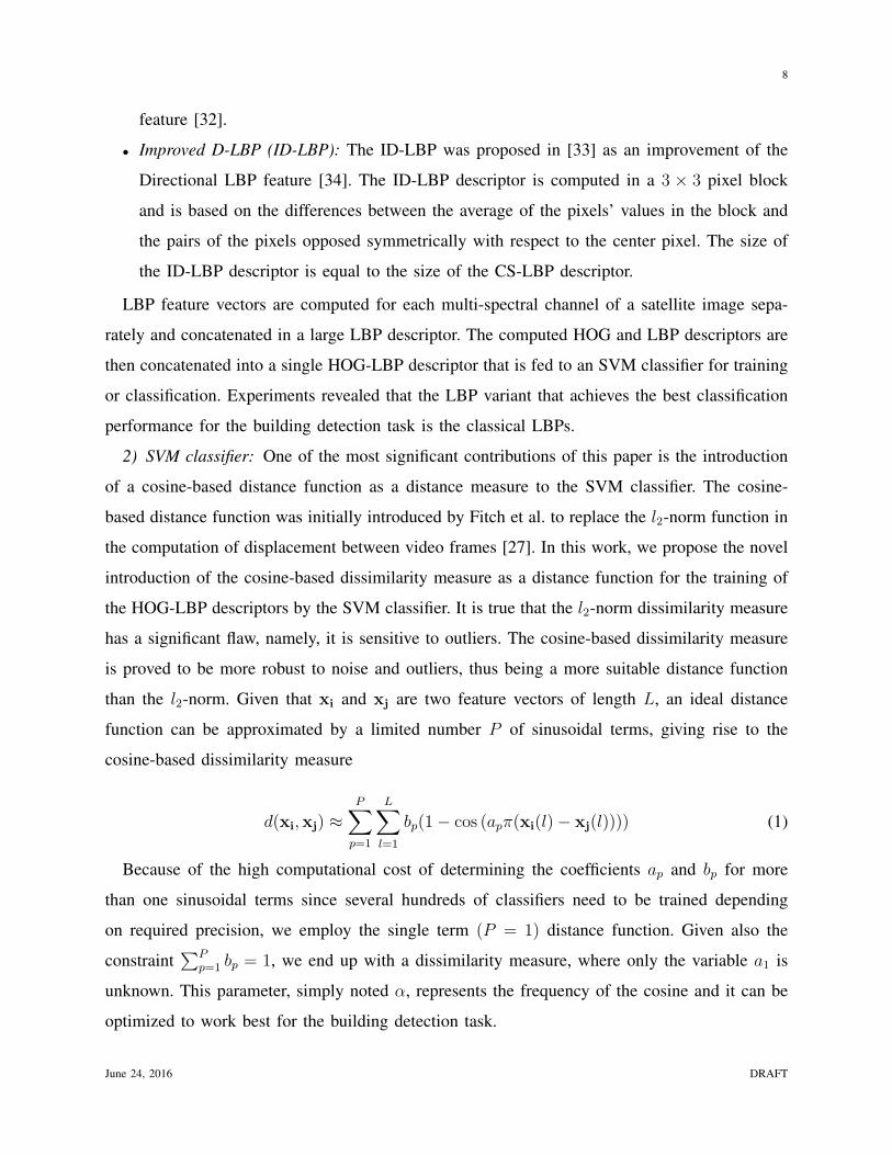
2) SVM classifier: One of the most significant contributions of this paper is the introduction

of a cosine-based distance function as a distance measure to the SVM classifier. The cosine-

based distance function was initially introduced by Fitch et al. to replace the l2-norm function in

the computation of displacement between video frames [27]. In this work, we propose the novel

introduction of the cosine-based dissimilarity measure as a distance function for the training of

the HOG-LBP descriptors by the SVM classifier. It is true that the l2-norm dissimilarity measure

has a significant flaw, namely, it is sensitive to outliers. The cosine-based dissimilarity measure

is proved to be more robust to noise and outliers, thus being a more suitable distance function

than the l2-norm. Given that xi and xj are two feature vectors of length L, an ideal distance

function can be approximated by a limited number P of sinusoidal terms, giving rise to the

cosine-based dissimilarity measure

d(xi,xj) ≈P∑

p=1

L∑l=1

bp(1− cos (apπ(xi(l)− xj(l)))) (1)

Because of the high computational cost of determining the coefficients ap and bp for more

than one sinusoidal terms since several hundreds of classifiers need to be trained depending

on required precision, we employ the single term (P = 1) distance function. Given also the

constraint∑P

p=1 bp = 1, we end up with a dissimilarity measure, where only the variable a1 is

unknown. This parameter, simply noted α, represents the frequency of the cosine and it can be

optimized to work best for the building detection task.

June 24, 2016 DRAFT

9

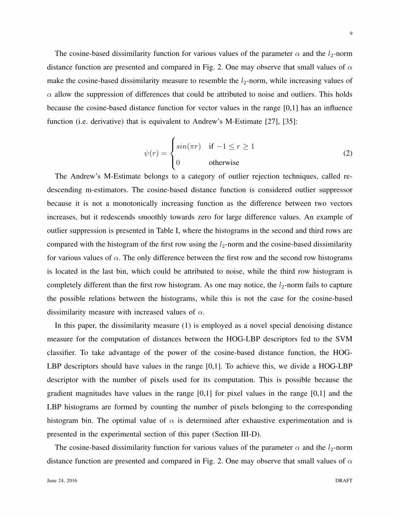
The cosine-based dissimilarity function for various values of the parameter α and the l2-norm

distance function are presented and compared in Fig. 2. One may observe that small values of α

make the cosine-based dissimilarity measure to resemble the l2-norm, while increasing values of

α allow the suppression of differences that could be attributed to noise and outliers. This holds

because the cosine-based distance function for vector values in the range [0,1] has an influence

function (i.e. derivative) that is equivalent to Andrew’s M-Estimate [27], [35]:

ψ(r) =

sin(πr) if −1 ≤ r ≥ 1

0 otherwise(2)

The Andrew’s M-Estimate belongs to a category of outlier rejection techniques, called re-

descending m-estimators. The cosine-based distance function is considered outlier suppressor

because it is not a monotonically increasing function as the difference between two vectors

increases, but it redescends smoothly towards zero for large difference values. An example of

outlier suppression is presented in Table I, where the histograms in the second and third rows are

compared with the histogram of the first row using the l2-norm and the cosine-based dissimilarity

for various values of α. The only difference between the first row and the second row histograms

is located in the last bin, which could be attributed to noise, while the third row histogram is

completely different than the first row histogram. As one may notice, the l2-norm fails to capture

the possible relations between the histograms, while this is not the case for the cosine-based

dissimilarity measure with increased values of α.

In this paper, the dissimilarity measure (1) is employed as a novel special denoising distance

measure for the computation of distances between the HOG-LBP descriptors fed to the SVM

classifier. To take advantage of the power of the cosine-based distance function, the HOG-

LBP descriptors should have values in the range [0,1]. To achieve this, we divide a HOG-LBP

descriptor with the number of pixels used for its computation. This is possible because the

gradient magnitudes have values in the range [0,1] for pixel values in the range [0,1] and the

LBP histograms are formed by counting the number of pixels belonging to the corresponding

histogram bin. The optimal value of α is determined after exhaustive experimentation and is

presented in the experimental section of this paper (Section III-D).

The cosine-based dissimilarity function for various values of the parameter α and the l2-norm

distance function are presented and compared in Fig. 2. One may observe that small values of α

June 24, 2016 DRAFT

10

make the cosine-based dissimilarity measure to resemble the l2-norm, while increasing values of

α allow the suppression of differences that could be attributed to noise and outliers. An example

of outlier suppression is presented in Table I, where the histograms in the second and third

rows are compared with the histogram of the first row using the l2-norm and the cosine-based

dissimilarity for various values of α. The only difference between the first row and the second

row histograms is located in the last bin, which could be attributed to noise, while the third row

histogram is completely different than the first row histogram. As one may notice, the l2-norm

fails to capture the possible relations between the histograms, while this is not the case for the

cosine-based dissimilarity measure with increased values of α.

In this paper, the dissimilarity measure (1) is employed as a novel special denoising distance

measure for the computation of distances between the HOG-LBP descriptors fed to the SVM

classifier. The optimal value of α is determined after exhaustive experimentation and is presented

in the experimental section of this paper (Section III-D).

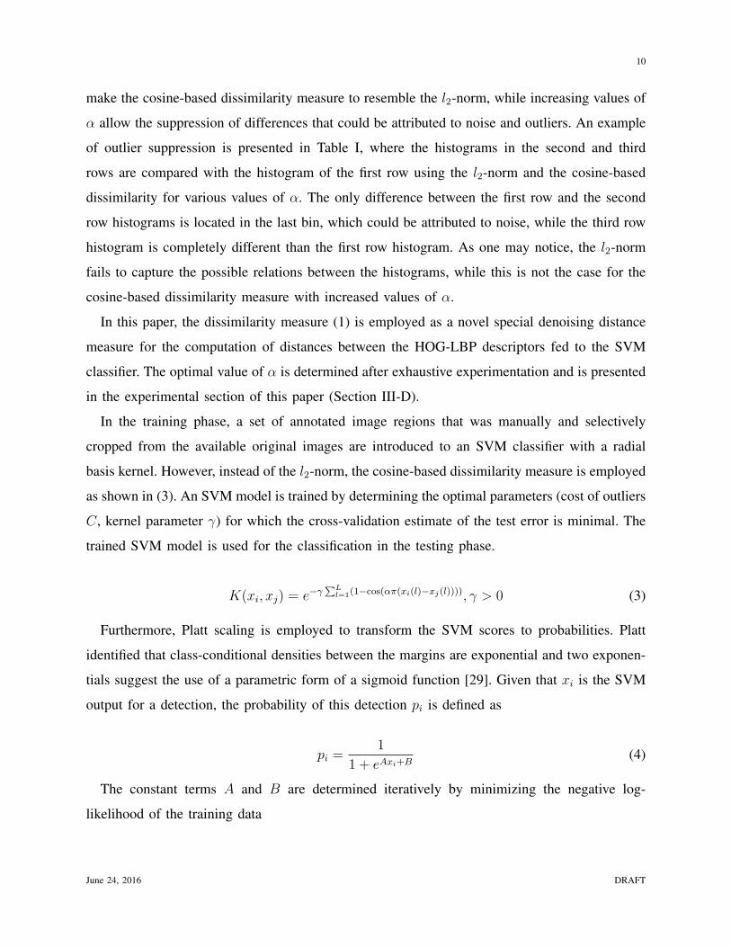
In the training phase, a set of annotated image regions that was manually and selectively

cropped from the available original images are introduced to an SVM classifier with a radial

basis kernel. However, instead of the l2-norm, the cosine-based dissimilarity measure is employed

as shown in (3). An SVM model is trained by determining the optimal parameters (cost of outliers

C, kernel parameter γ) for which the cross-validation estimate of the test error is minimal. The

trained SVM model is used for the classification in the testing phase.

K(xi, xj) = e−γ∑L

l=1(1−cos(απ(xi(l)−xj(l)))), γ > 0 (3)

Furthermore, Platt scaling is employed to transform the SVM scores to probabilities. Platt

identified that class-conditional densities between the margins are exponential and two exponen-

tials suggest the use of a parametric form of a sigmoid function [29]. Given that xi is the SVM

output for a detection, the probability of this detection pi is defined as

pi =1

1 + eAxi+B(4)

The constant terms A and B are determined iteratively by minimizing the negative log-

likelihood of the training data

June 24, 2016 DRAFT

11

min(−∑i

(tilog(pi) + (1− ti)log(1− pi))) (5)

where ti is equal to 0 for negative samples and 1 for positive samples. The purpose of the

minimization is to fit the sigmoid function to the training data. The sigmoid parameters are

determined using cross-validation on the training set. The idea behind the transformation of the

SVM scores to probabilities is two-fold, namely to enhance the meaning of the output of the

SVM classifier as instead of being the unbounded distance of a sample from the separating

hyperplane, it now expresses the probability of a sample to belong to the positive (“building”)

class and also to use a new probabilistic threshold to differentiate between building and non-

building regions, instead of the zero threshold that the standard SVM classifier assumes. As

it will be shown in Section III-B, Platt scaling increases the classification performance of the

HOG-LBP building detector.

In the testing phase, each test image is split in overlapping regions of multiple sizes (scales) and

a HOG-LBP descriptor is extracted for each image region. Afterwards, the HOG-LBP features

are classified to the building and non-building classes using the SVM model that was obtained in

the training phase of the methodology. The image regions that are classified by the SVM model

in the “building” class consist the initial rectangular image regions where buildings possibly

exist. The output of the HOG-LBP detector is sets of Cartesian coordinates and scales, which

define rectangular regions, possible candidates for the presence of buildings and corresponding

values that represent the confidence of the detections. Higher confidence is associated with higher

possibility of a true detection. Overlapping detections are merged in single detections using the

mean-shift algorithm, as proposed by Dalal [36]. The output of the mean-shift algorithm is used

as input to the second module of the proposed methodology [see Fig. 7(b)].

B. Region refinement module

Initially, the image is split in homogeneous regions by employing an unsupervised pixel

clustering technique. Vegetation and water masks are also extracted by employing a well-known

vegetation and a novel water index respectively. By identifying vegetation and water, we can

at a later stage discard building regions with a significant amount of pixels labeled as either

vegetation or water. Afterwards, we take advantage of the output of the HOG-LBP detector to

June 24, 2016 DRAFT

12

deduce the most probable to represent buildings image regions. These initial building candidates

are further processed to form the final building candidates.

1) Vegetation mask: One of the most accurate and well-known methods to detect vegetation in

multi-spectral images is the NDV I index [37]. The NDV I index has been successfully applied

in numerous remote sensing applications as an indicator of vegetated areas. This index takes

advantage of the near-infrared band that most satellites provide to identify where vegetation

exists. The rationale behind the use of NDV I is based on the fact that light is better absorbed

from vegetation than man-made structures. Consequently, this index produces high positive values

for vegetated regions and low positive or negative values for non-vegetated areas. NDV I is

computed using the near-infrared and red channels as shown below, where ρNIR and ρR are the

near-infrared and red channels respectively.

NDV I =ρNIR − ρRρNIR + ρR

(6)

NDV I is computed for each image pixel and then an optimal threshold is automatically

determined using Otsu’s method [38] in order to identify the pixels belonging to vegetation. The

threshold is computed based on the minimization of the intra-class variance of the NDVI values

between the pixels belonging to vegetation and those that do not. Pixels with values higher

than the value of threshold are labeled as vegetation. As a result, a binary mask is formed,

where vegetation pixels are highlighted. A morphological opening, followed by a morphological

closing operation, is finally applied to remove small “holes” or “islands” produced in the binary

vegetation mask [see Fig. 7(c)].

2) Water mask: Water extraction can be proved really useful for the task of building detection.

An urban area may not depict a significant number of water bodies, nevertheless the water in

urban environments is usually concentrated in swimming pools. Since swimming pools usually

have rectangular shapes, a building detection method that relies on shape features can mistakenly

consider swimming pools as candidate buildings. As a result, the detection of water bodies

and the removal of swimming pools can lead to false alarm reduction of a building detection

methodology. A commonly applied index that can differentiate the water class from other classes

is the Normalized Difference Water Index (NDWI) [39]. The NDWI index is computed using

the green and near-infrared channels as shown below, where ρG and ρNIR are the green and

June 24, 2016 DRAFT

13

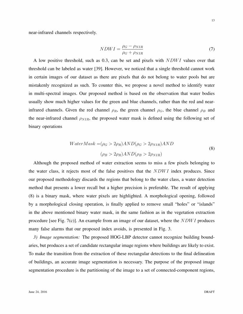
near-infrared channels respectively.

NDWI =ρG − ρNIR

ρG + ρNIR

(7)

A low positive threshold, such as 0.3, can be set and pixels with NDWI values over that

threshold can be labeled as water [39]. However, we noticed that a single threshold cannot work

in certain images of our dataset as there are pixels that do not belong to water pools but are

mistakenly recognized as such. To counter this, we propose a novel method to identify water

in multi-spectral images. Our proposed method is based on the observation that water bodies

usually show much higher values for the green and blue channels, rather than the red and near-

infrared channels. Given the red channel ρR, the green channel ρG, the blue channel ρB and

the near-infrared channel ρNIR, the proposed water mask is defined using the following set of

binary operations

WaterMask =(ρG > 2ρR)AND(ρG > 2ρNIR)AND

(ρB > 2ρR)AND(ρB > 2ρNIR)(8)

Although the proposed method of water extraction seems to miss a few pixels belonging to

the water class, it rejects most of the false positives that the NDWI index produces. Since

our proposed methodology discards the regions that belong to the water class, a water detection

method that presents a lower recall but a higher precision is preferable. The result of applying

(8) is a binary mask, where water pixels are highlighted. A morphological opening, followed

by a morphological closing operation, is finally applied to remove small “holes” or “islands”

in the above mentioned binary water mask, in the same fashion as in the vegetation extraction

procedure [see Fig. 7(c)]. An example from an image of our dataset, where the NDWI produces

many false alarms that our proposed index avoids, is presented in Fig. 3.

3) Image segmentation: The proposed HOG-LBP detector cannot recognize building bound-

aries, but produces a set of candidate rectangular image regions where buildings are likely to exist.

To make the transition from the extraction of these rectangular detections to the final delineation

of buildings, an accurate image segmentation is necessary. The purpose of the proposed image

segmentation procedure is the partitioning of the image to a set of connected-component regions,

June 24, 2016 DRAFT

14

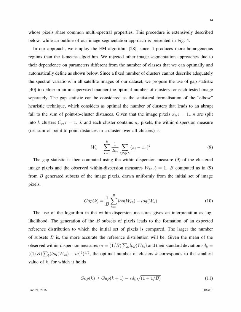
whose pixels share common multi-spectral properties. This procedure is extensively described

below, while an outline of our image segmentation approach is presented in Fig. 4.

In our approach, we employ the EM algorithm [28], since it produces more homogeneous

regions than the k-means algorithm. We rejected other image segmentation approaches due to

their dependence on parameters different from the number of classes that we can optimally and

automatically define as shown below. Since a fixed number of clusters cannot describe adequately

the spectral variations in all satellite images of our dataset, we propose the use of gap statistic

[40] to define in an unsupervised manner the optimal number of clusters for each tested image

separately. The gap statistic can be considered as the statistical formalisation of the “elbow”

heuristic technique, which considers as optimal the number of clusters that leads to an abrupt

fall to the sum of point-to-cluster distances. Given that the image pixels xi, i = 1...n are split

into k clusters Cr, r = 1...k and each cluster contains nr pixels, the within-dispersion measure

(i.e. sum of point-to-point distances in a cluster over all clusters) is

Wk =k∑

r=1

1

2nr

∑i,i′∈Cr

(xi − xi′)2 (9)

The gap statistic is then computed using the within-dispersion measure (9) of the clustered

image pixels and the observed within-dispersion measures Wkb, b = 1...B computed as in (9)

from B generated subsets of the image pixels, drawn uniformly from the initial set of image

pixels.

Gap(k) =1

B

B∑b=1

log(Wkb)− log(Wk) (10)

The use of the logarithm in the within-dispersion measures gives an interpretation as log-

likelihood. The generation of the B subsets of pixels leads to the formation of an expected

reference distribution to which the initial set of pixels is compared. The larger the number

of subsets B is, the more accurate the reference distribution will be. Given the mean of the

observed within-dispersion measures m = (1/B)∑

b log(Wkb) and their standard deviation sdk =

((1/B)∑

b(log(Wkb) − m)2)1/2, the optimal number of clusters k corresponds to the smallest

value of k, for which it holds

Gap(k) ≥ Gap(k + 1)− sdk√

(1 + 1/B) (11)

June 24, 2016 DRAFT

15

As a result, the optimal number of clusters is equal to the smallest value of k, for which

log(Wk) drops the farthest below the expected reference distribution [40]. The optimal number

of clusters k is determined by employing the gap statistic on the output of the k-means algorithm

for increasing values of k. The k-means algorithm is computationally faster than its EM coun-

terpart especially for large values of k, thus it is our selected clustering approach at this stage.

Afterwards, we use k to train k Gaussian models for the EM algorithm, which produces the final

image segmentation. Each pixel is labeled based on their colour values, where instead of the

Red-Green-Blue (RGB) colour space, the Hue-Saturation-Value (HSV) colour space is employed

for two main reasons; unlike the RGB colour space, the components of the HSV colour space are

independent of each other and the Hue (H) and Saturation (S) channels are intensity and shadow

invariant, thus the segmentation procedure based on HSV produces more homogeneous regions

within the underlying object boundaries. The near-infrared channel (NIR) is also employed,

along with the three HSV colour channels and participates in the image segmentation procedure.

Due to the fact that the H channel is expressed in degrees and has values in the range [0,360],

the transformation (12) is proposed so that the new values are in the range [0,1], as is the case

for the other three spectral channels (S,V ,NIR).

Hnew = 0.5− 0.5cos(πH

180) (12)

The set of regions that the EM algorithm outputs are further processed by applying a floodfill

operation that connects neighbouring pixels with the same label and stops at edge pixels detected

by the Canny algorithm. Such a procedure helps towards the accurate and robust identification

of object boundaries, since objects are usually distinguished by their edges. Unfortunately, this

procedure results in the over-segmentation of some image regions. To counter this, a region

merging procedure is afterwards applied, where each region with size smaller than a threshold

Tsmall is merged with one of its neighbouring regions, with which it has the best colour similarity.

The threshold Tsmall, which represents the area of the smallest region we wish to retain, should

be set to a value quite smaller than the smallest building that should be detected in order to

retrieve even non-homogeneous in colour buildings that were split in more than one regions.

The purpose of Tsmall is to get rid of the really small regions that increase the complexity of the

problem, while being insignificant for the building detection task. The remaining image regions

June 24, 2016 DRAFT

16

make up the pool of the candidate building regions that our proposed novel building region

detector will select [see Fig. 7(d)].

4) Building region detector: The purpose of the proposed novel building region detector is the

selection of the image regions that have the highest likelihood to correspond to buildings based

on the output of the HOG-LBP detector, their colour difference to their neighbouring regions and

their rectangularity. The proposed building region detector aims at achieving a transition from

the detections obtained using the HOG-LBP descriptors to the accurate pixel-based delineation

of the buildings in a satellite image. A block diagram of the building region detector along with

an example visualizing the employment of the proposed method on a HOG-LBP detection is

presented in Fig. 5. In the next paragraphs, we present and thoroughly explain the steps that the

proposed building region detector consists of.

The first step of the proposed methodology investigates the scoring of the image regions

that are formed by the image segmentation procedure. Let assume that the proposed HOG-LBP

detector is an ideal object detector, which possesses the following properties; (a) each detection

corresponds to one and only object, (b) the detected area is of rectangular shape and its centroid

is approximately the same as the centroid of the object (i.e. building) and finally (c) the size of

the object is associated to the scale in which the detection is found. Taking these properties into

consideration, we develop a novel approach for the scoring of image regions and the selection of

the best image regions as building candidates. From each HOG-LBP detection, represented as a

rectangular area AD with width and height l (width equals height in our case) and centroid OD,

a single image region AR, being the result of the image segmentation procedure described in

Section II-B3, with mean multi-spectral colour vector CR, centroid OR and bounded by a rotated

rectangle AB is selected as initial building candidate region based on the addition of four terms.

These terms are the amount of overlap between a region and the detection Mover, the region’s

rectangularity Mrect, the region’s colour difference to its neighbours Mcdiff and the distance

of the region’s centroid to the centroid of the detection Mdist. The purpose of employing and

summing all these terms is to aleviate problems where buildings may not have exact rectangular

shapes or their contrast with the background is weak. Next, we present how the above mentioned

terms are computed and why they are selected to form a scoring metric for the selection of an

image region as building candidate.

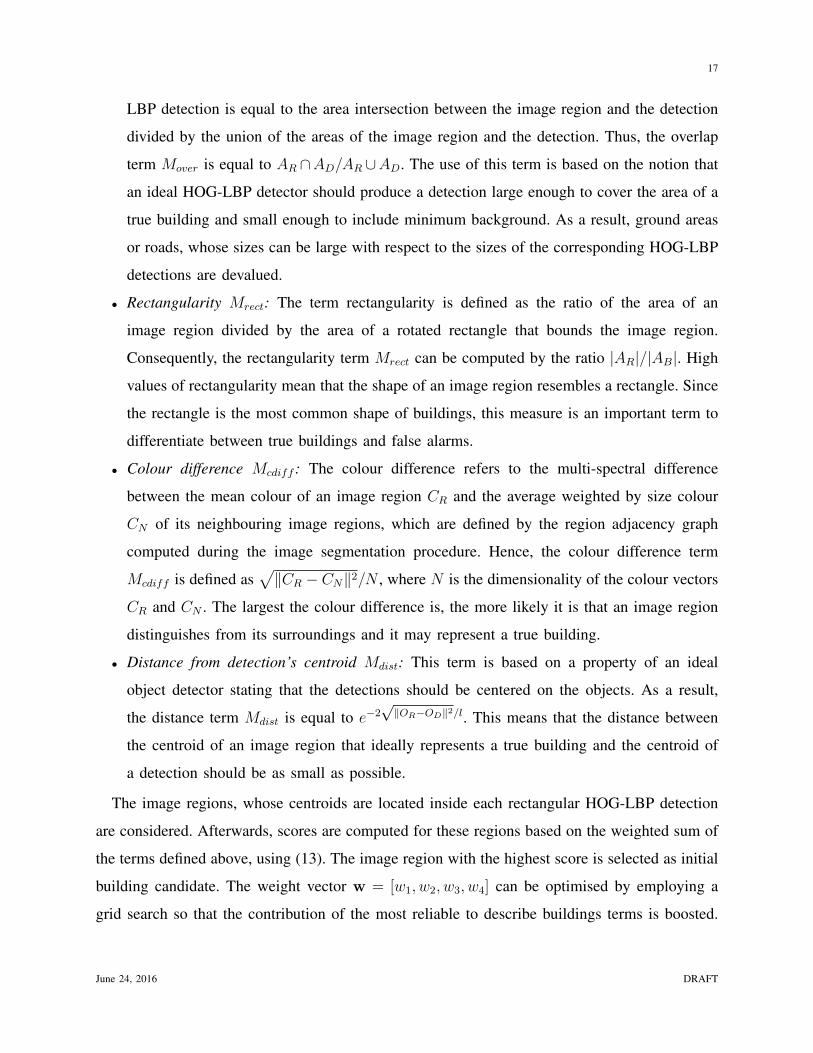
• Overlap with HOG-LBP detection Mover: The overlap of an image region with a HOG-

June 24, 2016 DRAFT

17

LBP detection is equal to the area intersection between the image region and the detection

divided by the union of the areas of the image region and the detection. Thus, the overlap

term Mover is equal to AR ∩AD/AR ∪AD. The use of this term is based on the notion that

an ideal HOG-LBP detector should produce a detection large enough to cover the area of a

true building and small enough to include minimum background. As a result, ground areas

or roads, whose sizes can be large with respect to the sizes of the corresponding HOG-LBP

detections are devalued.

• Rectangularity Mrect: The term rectangularity is defined as the ratio of the area of an

image region divided by the area of a rotated rectangle that bounds the image region.

Consequently, the rectangularity term Mrect can be computed by the ratio |AR|/|AB|. High

values of rectangularity mean that the shape of an image region resembles a rectangle. Since

the rectangle is the most common shape of buildings, this measure is an important term to

differentiate between true buildings and false alarms.

• Colour difference Mcdiff : The colour difference refers to the multi-spectral difference

between the mean colour of an image region CR and the average weighted by size colour

CN of its neighbouring image regions, which are defined by the region adjacency graph

computed during the image segmentation procedure. Hence, the colour difference term

Mcdiff is defined as√∥CR − CN∥2/N , where N is the dimensionality of the colour vectors

CR and CN . The largest the colour difference is, the more likely it is that an image region

distinguishes from its surroundings and it may represent a true building.

• Distance from detection’s centroid Mdist: This term is based on a property of an ideal

object detector stating that the detections should be centered on the objects. As a result,

the distance term Mdist is equal to e−2√

∥OR−OD∥2/l. This means that the distance between

the centroid of an image region that ideally represents a true building and the centroid of

a detection should be as small as possible.

The image regions, whose centroids are located inside each rectangular HOG-LBP detection

are considered. Afterwards, scores are computed for these regions based on the weighted sum of

the terms defined above, using (13). The image region with the highest score is selected as initial

building candidate. The weight vector w = [w1, w2, w3, w4] can be optimised by employing a

grid search so that the contribution of the most reliable to describe buildings terms is boosted.

June 24, 2016 DRAFT

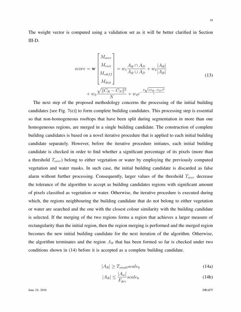
18

The weight vector is computed using a validation set as it will be better clarified in Section

III-D.

score = w

Mover

Mrect

Mcdiff

Mdist

= w1AR ∩ AD

AR ∪ AD

+ w2|AR||AB|

+ w3

√∥CR − CN∥2

N+ w4e

−2

√∥OR−OD∥2

l

(13)

The next step of the proposed methodology concerns the processing of the initial building

candidates [see Fig. 7(e)] to form complete building candidates. This processing step is essential

so that non-homogeneous rooftops that have been split during segmentation in more than one

homogeneous regions, are merged in a single building candidate. The construction of complete

building candidates is based on a novel iterative procedure that is applied to each initial building

candidate separately. However, before the iterative procedure initiates, each initial building

candidate is checked in order to find whether a significant percentage of its pixels (more than

a threshold Tover) belong to either vegetation or water by employing the previously computed

vegetation and water masks. In such case, the initial building candidate is discarded as false

alarm without further processing. Consequently, larger values of the threshold Tover decrease

the tolerance of the algorithm to accept as building candidates regions with significant amount

of pixels classified as vegetation or water. Otherwise, the iterative procedure is executed during

which, the regions neighbouring the building candidate that do not belong to either vegetation

or water are searched and the one with the closest colour similarity with the building candidate

is selected. If the merging of the two regions forms a region that achieves a larger measure of

rectangularity than the initial region, then the region merging is performed and the merged region

becomes the new initial building candidate for the next iteration of the algorithm. Otherwise,

the algorithm terminates and the region AR that has been formed so far is checked under two

conditions shown in (14) before it is accepted as a complete building candidate.

|AR| ≥ Tsmallscale0 (14a)

|AR| ≤|Aw|Fdev

scale0 (14b)

June 24, 2016 DRAFT

19

The use of these conditions is based on the fact that the HOG-LBP detector does not only

provide information about the location of a building, but also about the size of the building.

This information is stored at the scales of the detections and is employed in order to discard

candidate buildings that are less likely to correspond to true buildings. Given the scale scale0 of

the largest HOG-LBP detection that encloses region AR and the initial searching window Aw,

condition (14a) states that the area of the region AR should be larger or equal to the size of the

smallest region that is retained from the image segmentation procedure (i.e. Tsmall) multiplied

by scale0. Condition (14b) states that the size of the region AR should be smaller or equal to the

size of the largest rectangular HOG-LBP detection that encloses the region, divided by a factor

of deviation Fdev. The threshold Fdev has values in the range [0,1] and controls the size of the

accepted building candidates with respect to the size of a HOG-LBP detection, hence a large

threshold limits the range of building sizes the algorithm accepts. The final output of the initial

building candidate processing is a set of complete building candidates and their corresponding

measures of rectangularity that are employed in the final part of the methodology. An outline of

the algorithm that forms the complete building candidates is presented in Fig. 6.

Finally, the complete building candidates are tested whether their rectangularity is over a user-

defined threshold Trect. Ideally, we would like to retain building candidates with clear rectangular

shapes (i.e. high values of rectangularity) and hopefully, most falsely detected building candidates

will be discarded due to their low measures of rectangularity. The building candidates with

rectangularity higher than the threshold Trect form the final output of our proposed methodology

[see Fig. 7(f)]. The thresholds Tover, Fdev and Trect have been set using the validation dataset in

order to enhance the performance of the algorithm as it will be shown in Section III-D.

III. EXPERIMENTAL RESULTS

Our proposed methodology was tested on the Athens dataset of satellite images that is

introduced in Section III-A and results are presented and discussed. Initially, we introduce

and compare the variants of our proposed building detection method. Afterwards, our proposed

method is compared with state-of-the-art building detection approaches and object detection

methods that were adjusted and trained for the problem of building detection. Finally, we analyze

the sensitivity of the proposed method to changes in parameter configuration and we discuss the

advantages and limitations of our approach in the building detection task.

June 24, 2016 DRAFT

20

A. Dataset and Metrics

The Athens dataset consists of 29 multi-spectral orthorectified satellite images, depicting urban

areas of Athens in Greece. Most of these satellite images (17 in number) were captured by the

QuickBird satellite, have 4 multi-spectral channels (Red, Green, Blue and Near-infrared) and

present a spatial resolution of 0.6m per pixel, while 12 images were taken by the WorldView-2

satellite, have 8 multi-spectral channels (Red, Green, Blue, Yellow, Coastal, Red-Edge, NIR1,

NIR2) and present a spatial resolution of 0.5m per pixel. The images of the Athens dataset were

split in a validation set that consists of 5 images (3 QuickBird and 2 WorldView-2 images) and

a test set that consists of 24 images (14 QuickBird and 10 WorldView-2 images). The training

set was the same as the one employed in [21], consisting of 700 positive and 1400 negative

manually labeled image patches that were segmented from a QuickBird image, different from the

images used in the validation and test set. To be able to apply our proposed methodology to both

types of satellite images without modifications, we employ only the 4 common multi-spectral

channels. The test set contains 5105 buildings, annotated by human experts on separate ground

truth masks.

The evaluation of the methodologies on the dataset is performed both at object and pixel level.

We employ the common measures of recall, precision and F1-score to measure performance [41],

where

Recall =TP

TP + FN(15a)

Precision =TP

TP + FP(15b)

F1 − score =2 ∗Recall ∗ PrecisionRecall + Precision

(15c)

In (15), TP stands for true positives, FP stands for false positives and FN stands for false

negatives. In our building detection framework, the object-based results are computed by counting

the number of correctly detected and falsely identified buildings (TP and FP respectively). For

pixel-based results, TP stands for the number of correctly identified building pixels, FP stands

for the number of falsely labeled building pixels and FN stands for the number of missed

building pixels.

June 24, 2016 DRAFT

21

B. Comparison of HOG-LBP detector variants

In this section, we analyze and compare the HOG-LBP detector variants that we implemented

and tested on the satellite images of the Athens dataset. Our methodology is implemented using

C++ and the OpenCV library, from which several built-in functions have been employed. To

detect buildings of various sizes in an image, all tested methodologies employ searching windows

of multiple sizes (scales) ranging from 20×20 to 200×200 pixels. These sizes are adequate for

the detection of buildings with sizes in the interval 50-8000 m2, based on the resolution of

satellite images. The displacement between two consecutive searching windows (stride) is equal

to 5 pixels, while the ratio between two consecutive scales is selected to be equal to 1.1, as in

our previous work [21].

The first differentiation in our proposed methodology comes with the introduction of the

cosine-based dissimilarity measure as it was defined in (1). The computation of the distance

between the HOG-LBP descriptors using the l2-norm gives rise to the classical HOG-LBP

detector, denoted simply as HOG-LBP detector, while the computation of the distance between

the HOG-LBP descriptors using the cosine-based dissimilarity measure gives rise to the enhanced

HOG-LBP detector. The second and final differentiation of the HOG-LBP detectors concerns

the use of the Platt scaling. Instead of the typical SVM detector, where the detections with score

higher than the threshold of zero are accepted as positive detections, the use of the Platt scaling

allows the transformation of the SVM score to a probability. As a result, a new threshold can be

set to differentiate between positive and negative detections. The new threshold, which is equal

to 0.5, means that we accept only the detections that have at least 50% probability to belong

to the building class and has the advantage that it does not have to be determined manually by

experimentation on the dataset.

These two differentiations give rise to four HOG-LBP detector variants (M1-M4), which are

implemented and tested in the images of the Athens dataset. The performance of the methods at

object and pixel level are summarized in Table II, while the average object-based recall, precision

and F1-score and their corresponding standard deviations in the test set are presented in Fig. 9.

The standard deviations are employed as an indicator of the robustness of the tested methods

in the images of the Athens dataset. Since these images vary significantly in illumination and

spatial resolution (2 types of satellite are used), we believe it is important to compute such a

June 24, 2016 DRAFT

22

value.

From the results on the Athens dataset, one can deduce that the enhanced HOG-LBP detec-

tor with the employment of Platt scaling performs better than the other proposed HOG-LBP

detectors. More specifically, the cosine-based distance function boosts the performance of our

proposed method by 8.1% with respect to the measure of F1-score. An additional 4.5% increase

in F1-score is achieved by Platt scaling. Although a slight drop in recall is observed when the

cosine-based distance function and Platt scaling are employed, there is a significant increase in

precision that leads to an overall better performance of the Enhanced HOG-LBP detector with

Platt scaling (M4). The standard deviation of the Enhanced HOG-LBP detector with Platt scaling

is lower than the other HOG-LBP detector variants by at least 15%, meaning that this method is

more robust to intensity and spatial resolution variations than the other methods in the Athens

dataset.

As far as pixel-based performance is concerned, the Enhanced HOG-LBP detector with

Platt scaling achieves similar performance to the HOG-LBP detector with Platt scaling and

better performance than the cases, where no Platt scaling is introduced. Consequently, the

additions of the cosine-based distance function and Platt scaling are successful in their attempt

to remove noise and scale the SVM outputs respectively in a way to reduce false alarms and thus

increase precision in the building detection task. These conclusions are further backed up by the

comparison of the HOG-LBP variants in Fig. 10. The M4 method manages to reject most of

the false alarms present at road segments that the other HOG-LBP variants accept, while it also

achieves more precise boundaries around buildings. Moreover, all HOG-LBP variants (M1-M4)

are capable of identifying problematic cases of buildings with spectral variations in their rooftops

[see white circles in Fig. 10] or buildings partially covered by vegetation [see orange circles in

Fig. 10].

C. Comparison with other techniques

In this section, our proposed methodology is compared with other object and building detection

methodologies. We describe the implemented and tested methods and evaluate their performance

on the satellite images of our test set.

• Cascade classifier with HAAR features (M5): A cascade of boosted classifiers is a structure

of several simple classifiers, whose votes are aggregated to increase the performance of a

June 24, 2016 DRAFT

23

detector. Such a cascade classifier that employs HAAR features was initially proposed in

[42] and was later improved in [43]. The cascade classifier was trained and used for the

detection of buildings in the Athens dataset. All four types of boosting techniques were

tested, namely the Discrete Adaboost, the Real Adaboost, the Logitboost and the Gentle

Adaboost. Furthermore, the classifier was tested for increasing number of cascade stages

in order to identify which parameter configuration achieves the best performance on the

building detection task. The results are presented in Fig. 8(a), where one can deduce that the

Discrete Adaboost classifier with 16 cascade stages achieves slightly better results than the

Real Adaboost with 16 stages and much better results than other parameter configurations.

• Cascade classifier with LBP features (M6): This classifier employs the same idea as the

previously presented cascade classifier, with the only difference residing in the use of LBP

features instead of HAAR features. Similar to the HAAR cascade classifier, experiments

were run for all types of boosting techniques and several cascade stages in order to identify

which parameter configuration achieves the best performance on the building detection task.

The results are presented in Fig. 8(b), where one can deduce that the Logitboost classifier

with 17 cascade stages achieves slightly better results than the Gentle Adaboost with 17

stages and much better results than other parameter configurations.

• Fisherfaces (M7): Fisherfaces is a method proposed to replace the Eigenfaces method as

an alternative solution to the face recognition task by [44]. Using Fisher’s Discriminant

Analysis, class-specific dimensionality reduction is achieved in an attempt to increase the

discrimination between classes and thus, the performance of an object detector. Fisherfaces

were adjusted and employed for the task of building detection in the Athens dataset.

• Sirmacek et al. feature fusion (M8) [6]: A building detection methodology by fusing various

distinctive features is proposed in [6]. The authors employed Harris and FAST corner

features, GMSR regions and Gabor-filtering local features to identify building centers.

Unlike the other algorithms, this is the only method that cannot detect building candidate

regions but only building centers. Therefore, the performance of this methodology can only

be evaluated at the object level and not at the pixel level. The object-level evaluation is

based on single-pixel overlap of a computed building center with the ground truth building

area, since the method does not provide any knowledge of the scale of the building.

• Konstantinidis et al. HOG detector (M9) [21]: In our previous work, we employed the

June 24, 2016 DRAFT

24

HOG detector and used all multi-spectral information of a satellite image, concatenating

the HOG descriptors computed for each multi-spectral channel separately. Furthermore, an

optimal parameter configuration for the task of building detection was determined based on

the validation set.

• Chaudhuri et al. building detector (M10) [45]: A building detector based on Internal Gray

Variance (IGV) and morphology operations is proposed in [45]. IGV features are extracted

and the edge pixels that do not correspond to man-made objects are rejected. Then, shadow

detection is employed to remove false alarms and the remaining edges form the candidate

regions out of which, buildings are extracted [45]. We implemented their method with the

exception that their proposed shadow detection technique was replaced by the algorithm of

Liu et al. [46] for panchromatic images as their shadow detection technique was not clear

enough to be implemented. We experimented with various parameter values to find out that

the values proposed in their paper yield the best results in the Athens dataset.

The performance of the previously described methodologies (M5-M10) is evaluated at object

and pixel level in the Athens dataset and the total measures of recall, precision and F1-score

are summarized in Table II. Furthermore, the average object-based recall, precision and F1-score

and their corresponding standard deviations are presented in Fig. 9.

Methods M5-M9 can be described as object-based methods since no building delineation

is attempted. Therefore, the performance of these methods can be directly compared to the

performance of our proposed enhanced HOG-LBP detector with Platt scaling (M4). The results

at the object level show the superiority of our object-based building detector (M4) over the other

methods. More specifically, our proposed method achieves an increase in F1-score by 10.7%

over the second best method, which is the cascade classifier with LBP features (M6) and by

more than 23% over the third best method, being the Konstantinidis et al. building HOG detector

(M9). Worthy of notice is the almost perfect (marginally less than 1) recall of the Fisherfaces

method (M7). However, the low precision of method M7 leads to mediocre F1-score and thus,

mediocre performance in the Athens dataset. Our proposed algorithm (M4) achieves the lowest

standard deviation in F1-score with a value of 0.058, followed by the methods M5,M6 and

M9 that perform similarly with a slightly larger value of 0.067. This means that the method

M4 shows greater robustness than the other methods with respect to illumination and spatial

resolution changes present in the images of the Athens dataset.

June 24, 2016 DRAFT

25

A comparison of the pixel-based performance of the methods M4-M9 reveals that the cascade

boosted classifier with HAAR features (M5) achieves the best precision and F1-score. However,

the measure of recall is much lower than that of other methodologies, making it an undesirable

building detector in the Athens dataset. Konstantinidis et al. HOG detector (M9) achieves the

second best precision and F1-score, but its recall is not as high as the recall that our proposed

HOG-LBP detector (M4) achieves. The reason behind the low pixel-based precision of the

methodologies M4-M7 and M9 is attributed to the fact that these methods detect regions where

buildings are likely to exist and they cannot recognize and extract building boundaries.

A study of the tested methods M5-M9 and their corresponding results in the building detection

task reveal their weaknesses. HAAR features sum up intensities in rectangular regions and thus

they are sensitive to illumination changes, affecting significantly the results of building detection

in images being under various lightning conditions. Fisherfaces method relies on the assumption

that the classes can be linearly separated in an image subspace. However, this cannot be easily

guaranteed in several object detection tasks. Sirmacek et al. method (M8) relies on the fusion

of corner and gradient features. The images of the Athens dataset suffer from noise and low

contrast of buildings to background and therefore, this method fails to extract enough corners

to successfully identify building centers. Finally, the cascade classifier with LBP features (M6)

and the Konstantinidis et al. HOG detector (M9) are successful in discriminating buildings from

background but their performance is still outmatched by the complementary use of both HOG

and LBP features employed in the proposed building detector (M4).

Next, we compare our proposed methodology with the addition of the region refinement

procedure (M11) with another pixel-based building detection method (M10). These two methods

are capable of accurately identifying and extracting buildings from satellite images. The results

presented in Table II and Fig. 9 demonstrate the superiority of our proposed building detector

(M11) over the algorithm developed by Chaudhuri et al. (M10) both at object and pixel level.

More specifically, our method improves the object-based and pixel-based F1-score by almost

12.8% and 69% respectively in comparison with the performance of the methodology M10 in

the Athens dataset. Our methodology is inferior only in the object-based precision, where the

algorithm M10 achieves the highest object-based precision from all tested object and pixel-

based methodologies in the Athens dataset. Comparing the standard deviations, we conclude

that our proposed methodology (M11) achieves the lowest standard deviation in F1-score with

June 24, 2016 DRAFT

26

a value of 0.041, meaning that it is more robust than any other tested method, including the

method of Chaudhuri et al. (M10). The building detection results of our proposed building

detection framework (M11) and the algorithm of Chaudhuri et al. (M10) in two Quickbird and

one WorldView-2 satellite images of the Athens dataset are visualized in Fig. 12.

The inferior performance of the Chaudhuri et al. building detector (M10) in the Athens dataset

can be attributed to three main reasons. Firstly, the methodology is strongly affected by the

selection of a suitable building template that enhances the contrast between the buildings and

other objects in a satellite image. We experimented with various templates to get optimal results,

but a selection of a non-representative template can significantly affect the results. Secondly, noise

and low contrast present in the Athens dataset can severely affect the extraction of building edges

that play a key role to the performance of the building detector. Finally, in high-resolution satellite

images, shadow is present not only near buildings but also near other objects, such as tall trees

and fences. As a result, non-building edges can be wrongly assumed to belong to buildings,

leading to a drop in the performance of the building detector.

Next, our proposed pixel-based building extractor (M11) is compared with our proposed object-

based building detector (M4). The results show that the pixel-based performance of the algorithm

M11 is significantly better than the performance of the method M4, as several false detections

are removed and building boundaries are correctly identified. Unfortunately, some buildings are

lost in the process, leading to a drop in the pixel-based recall and the object-based performance

of the algorithm M11 in the Athens dataset. This loss of buildings can be attributed to the fact

that the quality of image segmentation can be severely degraded in cases of noise in the satellite

image or buildings with similar colour information to the background. Finally, there are some

buildings with irregular shapes that do not present high rectangularity values and therefore, they

are discarded either during the formation of the initial building candidates or by the employment

of the rectangularity threshold.

Finally, Fig. 10 compares the detections of the tested methodologies in a part of a satellite

images where buildings with spectral variations in their rooftops (i.e. buildings inside the white

circles) and buildings partially occluded by vegetation (i.e. buildings inside the orange circles)

exist. Results reveal that the cascade classifiers (methods M5 and M6), similar to the HOG-

LBP variants have no problem detecting such “problematic” cases of buildings. Unfortunately,

the cascade classifiers seem to miss a few “regular” buildings or inaccurately identify them

June 24, 2016 DRAFT

27

(i.e. significant portion of a detection is covered by background). The Fisherfaces method (M7)

also manages to identify “problematic” cases of buildings, however at the expence of producing

several false alarms around them. Sirmacek’s approach (M8), on the other hand, shows a problem

in identifying one of the buildings with spectral variations in its rooftop, while it also fails to

detect several “regular” buildings. Similarly, both Konstantinidis et al. HOG detector (M9) and

Chaudhuri et al. method (M10) fail to identify a building that presents spectral variations, while

both algorithms successfully identify buildings that are partially covered by vegetation. Finally,

our proposed methodology (M11) identifies correctly all the buildings that present either spectral

variations in their rooftops or are partially occluded by vegetation. This can be attributed to the

fact that the method M4 correctly captures such “problematic” cases of buildings and the region

refinement procedure does not reject them as false alarms.

D. Sensitivity to parameters

Initially, experiments were made in order to determine which LBP variant achieves the greatest

improvement in the performance of the building detector when it is combined with the HOG

descriptor. The results of the experimentation with the LBP variants are presented in Table III

and reveal that the best performance of our proposed building detector is achieved with the

classical LBP feature vectors, followed by the slightly worse performance of the uniform LBP

feature vectors.

We set the number of generated data subsets B that affect the accuracy of the computed gap

statistic equal to 20. Experiments revealed that the proposed methodology is robust to changes

to the number of generated data subsets B since high values affect slightly the accuracy of the

gap statistic, while increase significantly the computational time. Furthermore, the morphological

operations applied during the formation of the final vegetation and water masks are performed

using a square structuring element of size 5×5 in pixels. This size is large enough to suppress

small details and holes in the masks and small enough to avoid significant misclassification

errors. The parameters that affect the performance of the proposed building detector and should

be properly defined are the frequency of the cosine-based dissimilarity measure α, the factor of

deviation Fdev, the minimum area of accepted image regions in the image segmentation procedure

Tsmall, the percentage of building candidate’s pixels that should belong to either vegetation or

water so that the building candidate is discarded Tover, the weight vector w and the rectangularity

June 24, 2016 DRAFT

28

threshold Trect. These parameters are defined by experimentation on the 5 satellite images of

our validation set and chosen based on the optimization of the pixel-based performance of our

proposed building detector (M11).

The minimum area of an image region Tsmall should be set smaller than the size of the

smallest building, in order to take into account non-homogeneous rooftops. Since we have already

employed a HOG-LBP building detector, Tsmall can be set to a value proportional to the size

of the initial searching window of the HOG-LBP algorithm. The weight vector w is determined

by a grid search for component values in the range [0,1] with a step of 0.05. This is possible

because the absolute value of the weighted sum given by (13) is irrelevant for the comparison

between the image regions as we are only interested for which region this sum gets the highest

score. Experiments show that the most significant scoring term is the colour difference of an

image region to its neighbours, followed by the overlap of an image region and the corresponding

detection of the HOG-LBP algorithm. Finally, the parameter α that determines the frequency

of the cosine-based distance function varies in the range [0,1.99] with steps of 0.01. Table

IV presents the optimal parameter values that achieve the results presented in Table II. Fig.

11 illustrates the effects of varying the parameter values on the performance of the proposed

methodology on the validation set.

From Fig. 11, a few conclusions can be drawn. The selection of an appropriate value for the

frequency of the cosine-based dissimilarity measure α is of paramount importance. From Figs.

11 (a) and (b), it can be noticed that the performance of the proposed methodology increases only

for values of α smaller than 0.4. The optimal value of 0.09 for the parameter α means that the

amount of noise in the training set is not significant and slight variations in the computed HOG-

LBP descriptors are essential for the differentiation between positives and negatives. From Figs.

11 (c), (d) and (f), one can observe that our proposed methodology is quite robust in changes

of these parameters’ values. Most of the regions with low rectangularity scores have already

been rejected during the previous steps of the methodology and increasing the rectangularity

threshold does not lead to a significant increase in the accuracy of the algorithm. In cases where

the rectangularity threshold is set to too high values, a drop in the pixel-based performance of

the proposed method is observed. Finally, the size of the smallest accepted image region seems

to affect significantly the performance of the algorithm, as shown in Fig. 11 (e). This can be

attributed to the fact that our proposed method is quite sensitive to the quality of the image

June 24, 2016 DRAFT

29

segmentation, requiring an as accurate as possible image segmentation.

E. Limitations

Although our proposed methodology shows superior performance over other object-based and

pixel-based building detection methods, there are still some significant limitations. Firstly, the

results are significantly affected by the output of the HOG-LBP algorithm, meaning that buildings

lost by the HOG-LBP detector cannot be recovered in the next steps of the proposed method.

Secondly, the quality of image segmentation plays a crucial role to the building detection task.

Buildings that are not accurately segmented by our proposed image segmentation procedure may

not be selected by the region refinement procedure, thus being discarded by our proposed building

detector. Cases of falsely or partially extracted buildings can be enhanced by the presence of

noise and low contrast of buildings from background in satellite images. Although more than

one scoring terms are aggregated, as shown in (13), there can still be non-building regions that

achieve higher score than the building regions.

Finally, our methodology may fail to reject false positives that describe small road segments

or land patches (see blue areas in roads and land in Fig. 12 (d)). In such occasions, the extracted

image regions can present high rectangularity and strong contrast with the background, thus

mistakenly recognised as buildings. Such problems can however be alleviated if steps are taken

in the direction of segmenting a satellite image accurately, since then roads and land fields will

extend out of the HOG-LBP detections and they will be devalued by the scoring metric (13).

IV. CONCLUSIONS

In this paper, we propose a novel building detection methodology from satellite images. Our

method employs concatenated HOG and LBP features using a novel distance function in the

training and testing of the SVM classifier. Furthermore, we adopt a novel strategy to define

a robust threshold using Platt scaling to determine which detections are accepted as positives

and which are discarded as false alarms. The new threshold gives a significant boost to the

performance of the HOG-LBP detector. Finally, we propose a novel approach to accurately

detect building boundaries. The region refinement procedure is based on the result of an image

segmentation procedure, the use of the output of the HOG-LBP detector and the employment of

novel scoring metrics to determine the regions that are more likely to correspond to buildings.

June 24, 2016 DRAFT

30

Applying our proposed method to the Athens dataset of satellite images reveals the superiority

of the HOG-LBP detector over other object and building detection methodologies. The region

refinement procedure, although successful in its purpose to improve the pixel-based performance

of our building detector, faces problems keeping the high recall of the HOG-LBP detector, as

a few buildings are lost in the process. Likely most of these problems can be mitigated by an

accurate image segmentation procedure.

ACKNOWLEDGEMENTS

We would like to thank Dr. Beril Sirmacek for providing her code for our evaluation results.

This research has been co-financed by the European Union (European Social Fund-ESF) and

Greek national funds through the Operational Program “Education and Lifelong Learning” of the

National Strategic Reference Framework (NSRF)-Research Funding Program: THALIS-NTUA-

UrbanMonitor.

June 24, 2016 DRAFT

31

REFERENCES

[1] L. Theng, “Automatic building extraction from satellite imagery,” Engineering Letters, vol. 13, no. 3, Nov 2006.

[2] K. Karantzalos and D. Argialas, “A region-based level set segmentation for automatic detection of man-made objects from

aerial and satellite images,” Photogrammetric Engineering and Remote Sensing, vol. 75, no. 6, pp. 667–677, 2009.

[3] D. Singh, R. Maurya, A. Shukla, M. Sharma, and P. Gupta, “Building extraction from very high resolution multispectral

images using NDVI based segmentation and morphological operators,” in Students Conference on Engineering and Systems

(SCES), March 2012, pp. 1–5.

[4] T. Hermosilla, L. Ruiz, J. Recio, and J. Estornell, “Evaluation of automatic building detection approaches combining high

resolution images and LiDAR data,” Remote Sensing, vol. 3, no. 6, pp. 1188–1210, 2011.

[5] B. Sirmacek and C. Unsalan, “Urban-area and building detection using SIFT keypoints and graph theory,” IEEE

Transactions on Geoscience and Remote Sensing, vol. 47, no. 4, pp. 1156–1167, April 2009.

[6] ——, “A Probabilistic Framework to Detect Buildings in Aerial and Satellite Images,” IEEE Transactions on Geoscience

and Remote Sensing, vol. 49, no. 1, pp. 211–221, Jan 2011.

[7] P. Hough, “Method and means for recognizing complex patterns,” U.S. Patent 3,069,654, Dec 1962.

[8] T. Kim and J. Muller, “Development of a graph-based approach for building detection,” Image and Vision Computing,

vol. 17, no. 1, pp. 3–14, 1999.

[9] D. Haverkamp, “Automatic building extraction from IKONOS imagery,” in Proceedings of ASPRS, 2004.

[10] D. Woo, Q. Nguyen, Q. Nguyen Tran, D. Park, and Y. Jung, “Building detection and reconstruction from aerial images,”

in ISPRS Congress, Beijing, 2008.

[11] S. Vinson, L. Cohen, and F. Perlant, “Extraction of rectangular buildings in aerial images,” in Proceedings of Scandinavian

Conference on Image Analysis (SCIA), 2001.

[12] K. Karantzalos and N. Paragios, “Recognition-driven two-dimensional competing priors toward automatic and accurate

building detection,” IEEE Transactions on Geoscience and Remote Sensing, vol. 47, no. 1, pp. 133–144, Jan 2009.

[13] O. Benarchid, N. Raissouni, S. Adib, A. Abbous, A. Azyat, N. Achhab, M. Lahraoua, and A. Chahboun, “Building

extraction using object-based classification and shadow information in very high resolution multispectral images, a case

study: Tetuan, Morocco,” Canadian Journal on Image Processing and Computer Vision, vol. 4, no. 1, Jan 2013.

[14] S. Kluckner and H. Bischof, “Image-based building classification and 3d modeling with super-pixels,” in Proceedings of

International Society for Photogrammetry and Remote Sensing, Photogrammetric Computer Vision and Image Analysis,

2010.

[15] A. Shackelford and C. Davis, “A combined fuzzy pixel-based and object-based approach for classification of high-resolution

multispectral data over urban areas,” IEEE Transactions on Geoscience and Remote Sensing, vol. 41, no. 10, pp. 2354–2363,

Oct 2003.

[16] Z. Sheng-hua, H. Jian-jun, and X. Wei-xin, “A new method of building detection from a single aerial photograph,” in 9th

International Conference on Signal Processing (ICSP), Oct 2008, pp. 1219–1222.

[17] C. Senaras, M. Ozay, and F. T. Y. Vural, “Building Detection With Decision Fusion,” IEEE Journal of Selected Topics in

Applied Earth Observations and Remote Sensing, vol. 6, no. 3, pp. 1295–1304, June 2013.

[18] D. Chai, W. Forstner, and M. Ying Yang, “Combine markov random fields and marked point processes to extract building

from remotely sensed images,” in ISPRS Annals of the Photogrammetry, Remote Sensing and Spatial Information Sciences,

2012, pp. 1219–1222.

June 24, 2016 DRAFT

32

[19] O. O. Karadag, C. Senaras, and F. T. Y. Vural, “Segmentation Fusion for Building Detection Using Domain-Specific

Information,” IEEE Journal of Selected Topics in Applied Earth Observations and Remote Sensing, vol. 8, no. 7, pp.

3305–3315, July 2015.

[20] J. Femiani, E. Li, A. Razdan, and P. Wonka, “Shadow-Based Rooftop Segmentation in Visible Band Images,” IEEE Journal

of Selected Topics in Applied Earth Observations and Remote Sensing, vol. 8, no. 5, pp. 2063–2077, May 2015.

[21] D. Konstantinidis, T. Stathaki, V. Argyriou, and N. Grammalidis, “A probabilistic feature fusion for building detection in

satellite images,” in Proceedings of the 10th International Conference on Computer Vision Theory and Applications, 2015,

pp. 205–212.

[22] N. Dalal and B. Triggs, “Histograms of oriented gradients for human detection,” in IEEE Conference on Computer Vision

and Pattern Recognition (CVPR), vol. 1, June 2005, pp. 886–893.

[23] T. Ojala, M. Pietikainen, and D. Harwood, “Performance evaluation of texture measures with classification based on

Kullback discrimination of distributions,” in International Conference on Pattern Recognition, vol. 1, Oct 1994, pp. 582–

585.

[24] ——, “A comparative study of texture measures with classification based on featured distributions,” Pattern Recognition,

vol. 29, no. 1, pp. 51–59, Jan 1996.

[25] X. Wang, T. Han, and S. Yan, “An HOG-LBP human detector with partial occlusion handling,” in International Conference

on Computer Vision, Sep 2009, pp. 32–39.

[26] J. Zhang, K. Huang, Y. Yu, and T. Tan, “Boosted local structured HOG-LBP for object localization,” in International

Conference on Computer Vision and Pattern Recognition (CVPR), June 2011, pp. 1393–1400.

[27] A. Fitch, A. Kadyrov, W. Christmas, and J. Kittler, “Fast Robust Correlation,” IEEE Transactions on Image Processing,

vol. 14, no. 8, pp. 1063–1073, 2005.

[28] A. Dempster, N. Laird, and D. Rubin, “Maximum Likelihood from Incomplete Data via the EM Algorithm,” Journal of

the Royal Statistical Society, vol. Series B 39, no. 1, pp. 1–38, 1977.

[29] J. Platt, “Probabilistic Outputs for Support Vector Machines and Comparisons to Regularized Likelihood Methods,” in

Advances in Large Margin Classifiers. MIT Press, 1999, pp. 61–74.

[30] F. Bianconi and A. Fernndez, “On the Occurrence Probability of Local Binary Patterns: A Theoretical Study,” Journal of

Mathematical Imaging and Vision, vol. 40, no. 3, pp. 259–268, 2011.

[31] M. Pietikainen, A. Hadid, G. Zhao, and T. Ahonen, “Local Binary Patterns for Still Images,” in Computer Vision Using

Local Binary Patterns, ser. Computational Imaging and Vision. Springer London, 2011, vol. 40, pp. 13–47.

[32] J. Xiao and G. Wu, “A Robust and Compact Descriptor Based on Center-Symmetric LBP,” in International Conference

on Image and Graphics (ICIG), Aug 2011, pp. 388–393.

[33] S. Junding, Z. Shisong, and W. Xiaosheng, “Image retrieval based on an improved CS-LBP descriptor,” in IEEE

International Conference on Information Management and Engineering (ICIME), April 2010, pp. 115–117.

[34] W. Xiaosheng and S. Junding, “An effective texture spectrum descriptor,” in International Conference on Information

Assurance and Security (IAS), vol. 2, Aug 2009, pp. 361–364.

[35] P. Huber, Robust Statistics, ser. Wiley Series in Probability and Statistics. New York: Wiley, 1981.

[36] N. Dalal, “Finding People in Images and Videos,” Ph.D. dissertation, National Polytechnique de Grenoble, July 2006.

[37] J. Rouse, R. Haas, J. Scheel, and D. Deering, “Monitoring Vegetation Systems in the Great Plains with ERTS,” in 3rd

Earth Resource Technology Satellite (ERTS) Symposium, vol. 1, 1974, pp. 48–62.

June 24, 2016 DRAFT

33

HOG-LBP

descriptor

SVM

classification

HOG-LBP detector

Vegetation

mask

Water

mask

Image

segmentation

Building region

detector

HOG-LBP

descriptor

SVM training

Image

Region refinement

Building

candidates

Training samples

Training phase Testing phase

SVM

model

Rectangular

detections

Platt

params

Fig. 1. Block diagram of our proposed methodology, along with the defined modules and their interactions.

[38] N. Otsu, “A Threshold Selection Method from Gray-Level Histograms,” IEEE Transactions on Systems, Man and

Cybernetics, vol. 9, no. 1, pp. 62–66, Jan 1979.

[39] S. McFeeters, “Using the Normalized Difference Water Index (NDWI) within a Geographic Information System to Detect

Swimming Pools for Mosquito Abatement: A Practical Approach,” Remote Sensing, vol. 5, pp. 3544–3561, 2013.

[40] R. Tibshirani, G. Walther, and H. T., “Estimating the number of clusters in a data set via the gap statistic,” Journal of the

Royal Statistical Society: Series B (Statistical Methodology), vol. 63, pp. 411–423, 2001.

[41] D. L. Olson and D. Delen, Advanced Data Mining Techniques, 1st ed. Springer Publishing Company, 2008, p. 138.

[42] P. Viola and M. Jones, “Rapid object detection using a boosted cascade of simple features,” in Proceedings of the IEEE

Conference on Computer Vision and Pattern Recognition (CVPR), vol. 1, 2001, pp. 511–518.

[43] R. Lienhart and J. Maydt, “An extended set of Haar-like features for rapid object detection,” in Proceedings of the

International Conference on Image Processing, vol. 1, 2002, pp. 900–903.

[44] P. N. Belhumeur, J. P. Hespanha, and D. J. Kriegman, “Eigenfaces vs. Fisherfaces: Recognition Using Class Specific Linear

Projection,” IEEE Transactions on Pattern Analysis and Machine Intelligence, vol. 19, no. 7, pp. 711–720, July 1997.

[45] D. Chaudhuri, N. K. Kushwaha, A. Samal, and R. C. Agarwal, “Automatic Building Detection From High-Resolution

Satellite Images Based on Morphology and Internal Gray Variance,” IEEE Journal of Selected Topics in Applied Earth

Observations and Remote Sensing, vol. 9, no. 5, pp. 1767–1779, May 2016.

[46] J. Liu, T. Fang, and D. Li, “Shadow Detection in Remotely Sensed Images Based on Self-Adaptive Feature Selection,”

IEEE Transactions on Geoscience and Remote Sensing, vol. 49, no. 12, pp. 5092–5103, Dec 2011.

June 24, 2016 DRAFT

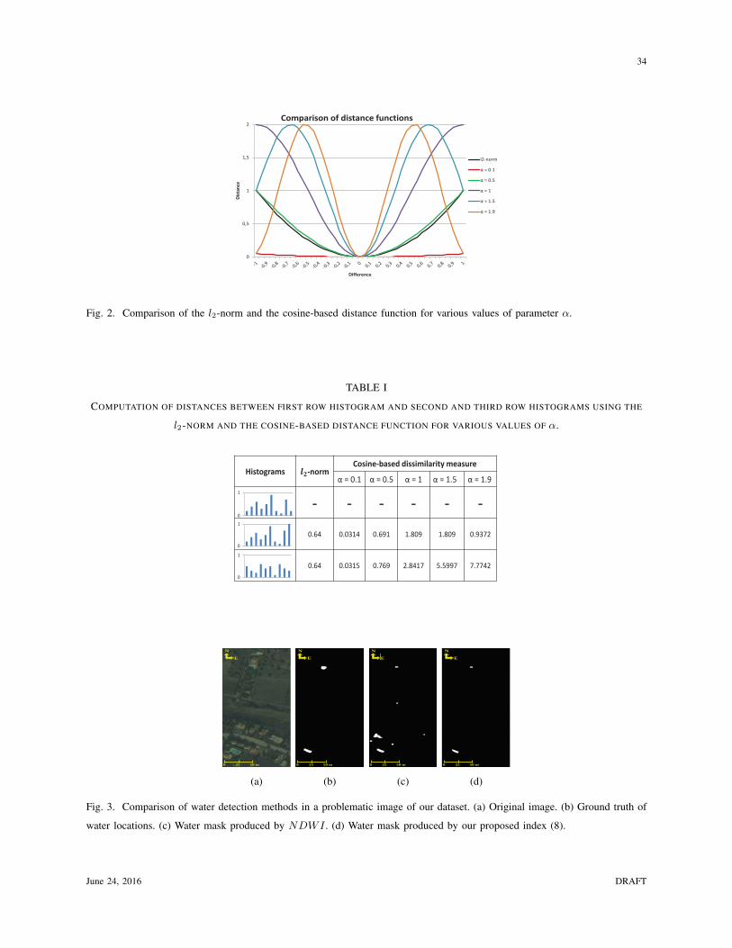
34

0

0,5

1

1,5

2

Dis

tan

ce

Difference

Comparison of distance functions

l2-norm

α = 0.1

α = 0.5

α = 1

α = 1.5

α = 1.9

Fig. 2. Comparison of the l2-norm and the cosine-based distance function for various values of parameter α.

TABLE I

COMPUTATION OF DISTANCES BETWEEN FIRST ROW HISTOGRAM AND SECOND AND THIRD ROW HISTOGRAMS USING THE

l2-NORM AND THE COSINE-BASED DISTANCE FUNCTION FOR VARIOUS VALUES OF α.

Histograms ��-norm Cosine-based dissimilarity measure

α = 0.1 α = 0.5 α = 1 α = 1.5 α = 1.9

- - - - - -

0.64 0.0314 0.691 1.809 1.809 0.9372

0.64 0.0315 0.769 2.8417 5.5997 7.7742

0

1

0

1

0

1

E

N

0 25 50 m

(a)

E

N

0 25 50 m

(b)

E

N

0 25 50 m

(c)

E

N

0 25 50 m

(d)

Fig. 3. Comparison of water detection methods in a problematic image of our dataset. (a) Original image. (b) Ground truth of

water locations. (c) Water mask produced by NDWI . (d) Water mask produced by our proposed index (8).

June 24, 2016 DRAFT

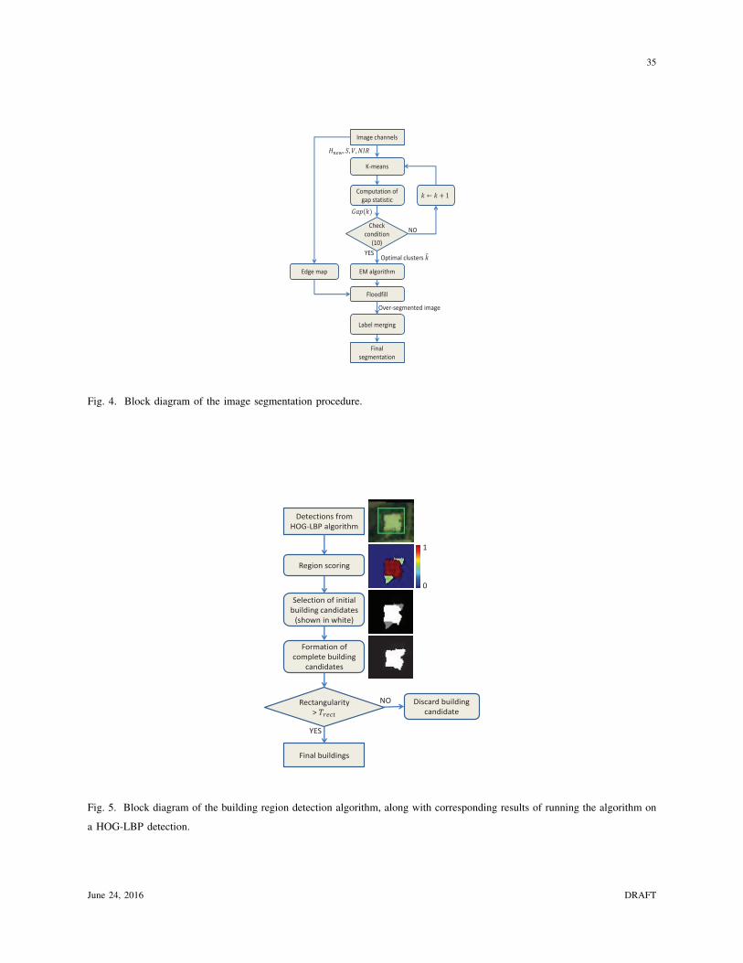
35

Computation of

gap statistic

Floodfill

� ← � + 1

Image channels

Final

segmentation

K-means

����, �, �, ���

Check

condition

(10)

���(�)

EM algorithm

Optimal clusters ��

NO

YES

Edge map

Label merging

Over-segmented image

Fig. 4. Block diagram of the image segmentation procedure.

Selection of initial

building candidates

(shown in white)

Detections from

HOG-LBP algorithm

Final buildings

Region scoring

Rectangularity

> �����

Formation of

complete building

candidates

NO

YES

Discard building

candidate

0

1

Fig. 5. Block diagram of the building region detection algorithm, along with corresponding results of running the algorithm on

a HOG-LBP detection.

June 24, 2016 DRAFT

36

Algorithm: Computation of complete building candidates

Input: Initial building candidates �� with corresponding scale ������ and rectangularity

�����, � = 1…�, Minimum size of image region T����� , Factor of deviation ���� , Area

of the initial searching window of HOG-LBP detector ��.

Output: Building candidates �� , � = 1…�.

for each region �� do:

if (!������ �!���"#"$��%&'#"�&(&�))

������ = 0

���� = �� �!

while ! ����

�� = �������ℎ !"#("�)

�� ∈ �� && �� = �������� !"#$#�%! �� ,��

&& !����� "�#� �$%$'��()*%$�)()�))

��� = ����� �� , ��

������ = ������ !"��#�$(���)

if ������ < �����

���� = ���

else

�� = ���

end

������ = max (������ , ������)

end

end

if (���� �� ≥ ������ ∗ ������ && ���� �� ≤ ��

����

∗ ������)

�� = ��

end

end

Fig. 6. Outline of the algorithm that forms the complete building candidates written in pseudocode.

TABLE II

TOTAL RECALL, PRECISION AND F1-SCORE OF THE TESTED METHODOLOGIES AT OBJECT AND PIXEL LEVEL IN THE

ATHENS DATASET. BEST VALUES SHOWN IN BOLD.

Method Object-based results Pixel-based results

Recall Precision F1-score Recall Precision F1-score

M1. HOG-LBP detector 0.978 0.645 0.777 0.964 0.108 0.194

M2. HOG-LBP detector + Platt scaling 0.951 0.746 0.836 0.945 0.121 0.215

M3. Enhanced HOG-LBP detector 0.964 0.745 0.84 0.94 0.112 0.2

M4. Enhanced HOG-LBP detector + Platt scaling 0.957 0.806 0.875 0.946 0.12 0.212

M5. Cascade classifier DAB with HAAR features (16 stages) 0.764 0.637 0.695 0.736 0.21 0.327

M6. Cascade classifier LB with LBP features (17 stages) 0.9 0.704 0.79 0.876 0.13 0.227

M7. Fischerface detector 0.999 0.451 0.621 0.998 0.089 0.163

M8. Sirmacek et al. (2011) 0.55 0.466 0.504 - - -

M9. Konstantinidis et al. (2015) 0.854 0.605 0.708 0.825 0.176 0.29

M10. Chaudhuri et al. (2015) 0.499 0.892 0.64 0.354 0.271 0.307

M11. Enhanced HOG-LBP detector + Platt scaling + Region

Refinement 0.719 0.724 0.722 0.555 0.488 0.519

June 24, 2016 DRAFT

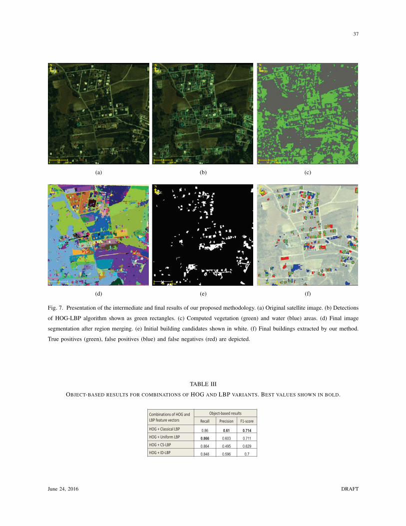
37

E

N

0 50 100 m

(a)

E

N

0 50 100 m

(b)

E

N

0 50 100 m

(c)

E

N

0 50 100 m

(d)

E

N

0 50 100 m

(e)

E

N

0 50 100 m

(f)

Fig. 7. Presentation of the intermediate and final results of our proposed methodology. (a) Original satellite image. (b) Detections

of HOG-LBP algorithm shown as green rectangles. (c) Computed vegetation (green) and water (blue) areas. (d) Final image

segmentation after region merging. (e) Initial building candidates shown in white. (f) Final buildings extracted by our method.

True positives (green), false positives (blue) and false negatives (red) are depicted.

TABLE III

OBJECT-BASED RESULTS FOR COMBINATIONS OF HOG AND LBP VARIANTS. BEST VALUES SHOWN IN BOLD.

Combinations of HOG and

LBP feature vectors

Object-based results

Recall Precision F1-score

HOG + Classical LBP 0.86 0.61 0.714

HOG + Uniform LBP 0.866 0.603 0.711

HOG + CS-LBP 0.864 0.495 0.629

HOG + ID-LBP 0.848 0.596 0.7

June 24, 2016 DRAFT

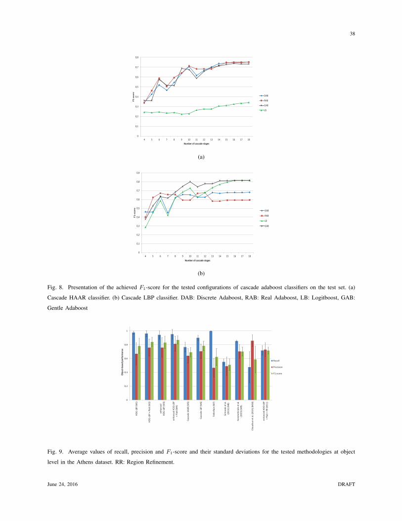
38

0

0,1

0,2

0,3

0,4

0,5

0,6

0,7

0,8

4 5 6 7 8 9 10 11 12 13 14 15 16 17 18

F1

-sco

re

Number of cascade stages

DAB

RAB

GAB

LB

(a)

0

0,1

0,2

0,3

0,4

0,5

0,6

0,7

0,8

0,9

4 5 6 7 8 9 10 11 12 13 14 15 16 17 18

F1

-sco

re

Number of cascade stages

DAB

RAB

LB

GAB

(b)

Fig. 8. Presentation of the achieved F1-score for the tested configurations of cascade adaboost classifiers on the test set. (a)

Cascade HAAR classifier. (b) Cascade LBP classifier. DAB: Discrete Adaboost, RAB: Real Adaboost, LB: Logitboost, GAB:

Gentle Adaboost

0

0,2

0,4

0,6

0,8

1

HO

G-L

BP

(M

1)

HO

G-L

BP

+ P

latt

(M

2)

en

ha

nce

d

HO

G-L

BP

(M

3)

en

ha

nce

d H

OG

-LB

P

+ P

latt

(M

4)

Ca

sca

de

HA

AR

(M

5)

Ca

sca

de

LB

P (

M6

)

Fis

he

rfa

ce (

M7

)

Sir

ma

cek

et

al.

(20

11

) (Μ

8)

Ko

nst

an

tin

idis

et

al.

(20

13

) (Μ

9)

Ch

au

dh

uri

et

al.

(2

01

5)

(Μ1

0)

en

ha

nce

d H

OG

-LB

P

+ P

latt

+ R

R (

Μ1

1)

Ob

ject

-ba

sed

pe

rfo

rma

nce

Recall

Precision

F1-score

Fig. 9. Average values of recall, precision and F1-score and their standard deviations for the tested methodologies at object

level in the Athens dataset. RR: Region Refinement.

June 24, 2016 DRAFT

39

E

N

0 25 50 m

(a)

E

N

0 25 50 m

(b)

E

N

0 25 50 m

(c)

E

N

0 25 50 m

(d)

E

N

0 25 50 m

(e)

E

N

0 25 50 m

(f)

E

N

0 25 50 m

(g)

E

N

0 25 50 m

(h)

E

N

0 25 50 m

(i)

E

N

0 25 50 m

(j)

E

N

0 25 50 m

(k)

E

N

0 25 50 m

(l)

Fig. 10. Comparison of the tested methodologies in a part of a satellite image depicting buildings with spectral variations in

their rooftops (white circles) and buildings covered partially by vegetation (orange circles). The initial image is presented in (a),

while the corresponding results of algorithms M1-M11 are shown in (b)-(l).

TABLE IV

PARAMETER SETTINGS FOR THE PROPOSED APPROACH.

Parameter Value

Frequency of cosine-based measure (�) 0.09

Subsets of data for gap statistic (�) 20

Minimum image region (������) 30 pixels

Factor of deviation (����) 0.45

Overlap threshold with vegetation or water (�����) 30%

Weight vector � [0.4,0.1,0.8,0.1]

Rectangularity threshold (�����) 0.4

June 24, 2016 DRAFT

40

0

0,1

0,2

0,3

0,4

0,5

0,6

0,7

0,8

0,9

1

0,0

1

0,0

6

0,1

1

0,1

6

0,2

1

0,2

6

0,3

1

0,3

6

0,4

1

0,4

6

0,5

1

0,5

6

0,6

1

0,6

6

0,7

1

0,7

6

0,8

1

0,8

6

0,9

1

0,9

6

1,0

1

1,0

6

1,1

1

1,1

6

1,2

1

1,2

6

1,3

1

1,3

6

1,4

1

1,4

6

1,5

1

1,5

6

1,6

1

1,6

6

1,7

1

1,7

6

1,8

1

1,8

6

1,9

1

1,9

6

Ob

jce

t-b

ase

d p

erfo

rm

an

ce

Frequency of cosine-based dissimilarity measure α

Recall Enhanced HOG-LBP

Precision Enhanced HOG-LBP

F1-score Enhanced HOG-LBP

Recall HOG-LBP

Precision HOG-LBP

F1-score HOG-LBP

(a)

0

0,1

0,2

0,3

0,4

0,5

0,6

0,7

0,8

0,9

1

0,0

1

0,0

6

0,1

1

0,1

6

0,2

1

0,2

6

0,3

1

0,3

6

0,4

1

0,4

6

0,5

1

0,5

6

0,6

1

0,6

6

0,7

1

0,7

6

0,8

1

0,8

6

0,9

1

0,9

6

1,0

1

1,0

6

1,1

1

1,1

6

1,2

1

1,2

6

1,3

1

1,3

6

1,4

1

1,4

6

1,5

1

1,5

6

1,6

1

1,6

6

1,7

1

1,7

6

1,8

1

1,8

6

1,9

1

1,9

6

Pix

el-

ba

se

d p

erf

orm

an

ce

Frequency of cosine-based dissimilarity measure α

Recall Enhanced HOG-LBP

Precision Enhanced HOG-LBP

F1-score Enhanced HOG-LBP

Recall HOG-LBP

Precision HOG-LBP

F1-score HOG-LBP

(b)

0

0,1

0,2

0,3

0,4

0,5

0,6

0,7

5 10 15 20 25 30 35 40 45 50 55 60 65 70 75 80 85 90 95 100

Pix

el-

ba

se

d p

erfo

rm

an

ce

hreshold (Tover) of number of vegetation or water pixels (%)

Recall

Precision

F1-score

(c)

0

0,1

0,2

0,3

0,4

0,5

0,6

0,05 0,1 0,15 0,2 0,25 0,3 0,35 0,4 0,45 0,5 0,55 0,6 0,65 0,7 0,75 0,8 0,85 0,9 0,95 1

Pix

el-

ba

sed

pe

rfo

rma

nce

Factor of deviation (Fdev)

Recall

Precision

F1-score

(d)

0,4

0,42

0,44

0,46

0,48

0,5

0,52

0,54

10 20 30 40 50 60 70 80 90 100

Pix

el-

ba

se

d p

erf

orm

an

ce

Size of smallest accepted image region (Tsmall)

Recall

Precision

F1-score

(e)

0

0,1

0,2

0,3

0,4

0,5

0,6

0,7

0,8

0 0,05 0,1 0,15 0,2 0,25 0,3 0,35 0,4 0,45 0,5 0,55 0,6 0,65 0,7 0,75 0,8 0,85 0,9 0,95

Pix

el-

ba

se

d p

erf

orm

an

ce

Rectangularity threshold (Trect)

Recall

Precision

F1-score

(f)

Fig. 11. Performance of our proposed methodology on the validation set for different parameter settings. (a) Effect of frequency

α on object-based performance. (b) Effect of frequency α on pixel-based performance. (c) Effect of overlap threshold with

vegetation and water Tover , (d) effect of factor of deviation Fdev , (e) effect of size of smallest accepted region Tsmall and (f)

effect of rectangularity threshold Trect on pixel-based performance.

June 24, 2016 DRAFT

41

E

N

0 50 100 m

(a)

E

N

0 50 100 m

(b)

E

N

0 50 100 m

(c)

E

N

0 50 100 m

(d)

E

N

0 50 100 m

(e)

E

N

0 50 100 m

(f)

E

N

0 50 100 m

(g)

E

N

0 50 100 m

(h)

E

N

0 50 100 m

(i)

Fig. 12. Comparison of our proposed methodology and the method proposed by Chaudhuri et al. [45] in 3 images of the Athens

dataset. (a),(b) Original QuickBird images. (c) Original WorldView-2 image. (d)-(f) Detected buildings from our method (M11)

for images (a)-(c) respectively. (g)-(i) Detected buildings from the method of Chaudhuri et al. (M10) for images (a)-(c). True

positive pixels are shown in green, false positive pixels are shown in blue and missed true positive pixels are presented in red.

June 24, 2016 DRAFT