c 2014 by Tao Yang. All rights reserved. - IDEALS
162
c 2014 by Tao Yang. All rights reserved.
Transcript of c 2014 by Tao Yang. All rights reserved. - IDEALS

c© 2014 by Tao Yang. All rights reserved.
FEEDBACK PARTICLE FILTER AND ITS APPLICATIONS
BY
TAO YANG
DISSERTATION
Submitted in partial fulfillment of the requirementsfor the degree of Doctor of Philosophy in Mechanical Engineering
in the Graduate College of theUniversity of Illinois at Urbana-Champaign, 2014
Urbana, Illinois
Doctoral Committee:
Professor Prashant G. Mehta, Chair and Director of ResearchProfessor Tamer BasarProfessor Venugopal V. VeeravalliProfessor Pierre Moulin
Abstract
The purpose of nonlinear filtering is to extract useful information from noisy sensor data. It finds applications in all
disciplines of science and engineering, including tracking and navigation, traffic surveillance, financial engineering,
neuroscience, biology, robotics, computer vision, weather forecasting, geophysical survey and oceanology, etc.
This thesis is particularly concerned with the nonlinear filtering problem in the continuous-time continuous-valued
state-space setting (diffusion). In this setting, the nonlinear filter is described by the Kushner-Stratonovich (K-S)
stochastic partial differential equation (SPDE). For the general nonlinear non-Gaussian problem, no analytical expres-
sion for the solution of the SPDE is available. For certain special cases, finite-dimensional solution exists and one
such case is the Kalman filter. The Kalman filter admits an innovation error-based feedback control structure, which
is important on account of robustness, cost efficiency and ease of design, testing and operation. The limitations of
Kalman filters in applications arise because of nonlinearities, not only in the signal models but also in the observation
models. For such cases, Kalman filters are known to perform poorly. This motivates simulation-based methods to
approximate the infinite-dimensional solution of the K-S SPDE. One popular approach is the particle filter, which is
a Monte Carlo algorithm based on sequential importance sampling. Although it is potentially applicable to a general
class of nonlinear non-Gaussian problems, the particle filter is known to suffer from several well-known drawbacks,
such as particle degeneracy, curse of dimensionality, numerical instability and high computational cost. The goal of
this dissertation is to propose a new framework for nonlinear filtering, which introduces the innovation error-based
feedback control structure to the particle filter. The proposed filter is called the feedback particle filter (FPF).
The first part of this dissertation covers the theory of the feedback particle filter. The filter is defined by an
ensemble of controlled, stochastic, dynamic systems (the “particles”). Each particle evolves under feedback control
based on its own state, and the empirical distribution of the ensemble. The feedback control law is obtained as the
solution to a variational problem, in which the optimization criterion is the Kullback-Leibler divergence between the
actual posterior, and the common posterior of any particle. The following conclusions are obtained for diffusions with
continuous observations: 1) The optimal control solution is exact: The two posteriors match exactly, provided they
are initialized with identical priors. 2) The optimal filter admits an innovation error-based gain feedback structure.
3) The optimal feedback gain is obtained via a solution of an Euler-Lagrange boundary value problem; the feedback
ii

gain equals the Kalman gain in the linear Gaussian case. The feedback particle filter offers significant variance
improvements when compared to the bootstrap particle filter; in particular, the algorithm can be applied to systems
that are not stable. No importance sampling or resampling is required, and therefore the filter does not suffer sampling-
related issues and incurs low computational burden.
The theory of the feedback particle filter is first developed for the continuous-time continuous-valued state-space
setting. Its extensions to two other settings are also studied in this dissertation. In particular, we introduce feedback
particle filter-based solutions for: i) estimating a continuous-time Markov chain with noisy measurements, and ii) the
continuous-discrete time filtering problem. Both algorithms are shown to admit an innovation error-based feedback
control structure.
The second part of this dissertation concerns the extensions of the feedback particle filter algorithms to address ad-
ditional uncertainties. In particular, we consider the nonlinear filtering problem with i) model uncertainty, and ii) data
association uncertainty. The corresponding feedback particle filter algorithms are referred to as the interacting multiple
model-feedback particle filter (IMM-FPF) and the probabilistic data association-feedback particle filter (PDA-FPF).
The proposed algorithms are shown to be the nonlinear non-Gaussian generalization of their classic Kalman filter-
based counterparts. One remarkable conclusion is that the proposed IMM-FPF and PDA-FPF algorithm retains the
innovation error-based feedback structure even for the nonlinear non-Gaussian case. The results are illustrated with
the aid of numerical simulations.
iii

To my parents.
iv
Acknowledgments
Above all I would like to thank my advisor, Professor Prashant G. Mehta, for his infinite support, enthusiasm, en-
couragement and guidance through my doctoral study at the University of Illinois at Urbana-Champaign. Special
thanks also go to Professor Sean P. Meyn at the University of Florida for his directions and insights on many of the
research works included in this thesis. I also greatly appreciate the guidance from Professor Henk A. P. Blom at the
Delft University of Technology and National Aerospace Laboratory in Amsterdam, the Netherlands. I’ve benefited a
lot from his instructive comments as well as his great passion about scientific research. I feel lucky and privileged
to have worked with them in the past few years. I would like to thank Professor Tamer Basar, Professor Venugopal
V. Veeravalli, and Professor Pierre Moulin for serving on my committee and providing valuable suggestions. I feel
honored to have them as my defense committee.
I would like to thank the Coordinated Science Laboratory (CSL) for providing me the working space and research
facilities. The CSL is an exceptional place to be a graduate student at. The research environment is interdisciplinary
and spectacular. I would like to thank the staff and students of CSL for maintaining such a friendly atmosphere. I
especially wish to thank Angie Ellis and Becky Lonberger for their help. I am also grateful to the Department of
Mechanical Science and Engineering for admitting me to the PhD program. I would like to thank Kathy Smith for her
patience to answer all my questions related to the graduate program. This research was funded by several institutions.
I am deeply grateful to the National Science Foundation, and the Air Force Office of Scientific Research for their
support of my entire doctoral program.
I would not survive the long journey without my friends along the way. I would like to thank Kun Deng for his
selfless help and valuable guidance ever since I met him. It is really a blessing to have him both as an academic mentor
and a life counselor. I would like to thank Yu Sun, Huibing Yin and Dayu Huang, Bo Tan for their useful suggestions
on my research and career development. I would like to thank Adam Tilton who has been an inspiring lab mate and
an amazing entrepreneur. Thank you for saving me from the bicycle trip at Montreal, Canada. I would like to thank
the brain trust whom I sat with everyday. Thank you Shane Ghiotto, Chi Zhang, Rohan Arora, Amir taghvaei, Sahand
Hariri, Geng Huang, Krishna Medarametla for all the good collaboration and friendship.
I would like to thank Xun Gong, Yunwen Xu, Jiamin Xu, Rui Wu, Quan Geng, Mindi Yuan, Qiaomin Xie, Ji Zhu,
v

Yun Li, Lili Su, Ge Yu, Xiaoyu Guang, Yifei Yang for all the meals and laughters we have together. I would like thank
my basketball buddies at the U of I for the good memories on and off the court. I would also like to thank my small
groups at both TCBC and CFC. It is my honor to have the fellowship with you and your prayers have always been a
great support to me. All your friendship is greatly appreciated and treasured.
I am grateful to my girlfriend, Weiran Zhao, for showing up in my life and falling love with me. It is one of the
most beautiful things that have ever happened in my life. It would be impossible for me to finish this work without
you. I would also like to thank my parents, Yajian Yang and Jianqiu Tao, for their deep and unconditional love along
the way. They give me the freedom to pursue my own interest and the trust to make decisions. They also teach me
the value of hard working, time-managing, and self-control. Their supports and encouragements always give me the
strength and perseverance to deal with any difficulties I encountered in my research and life.
Lastly, I would like to thank God my savior, for your word is a lamp to my feet and a light to my path.
vi

Table of Contents
List of Figures . . . . . . . . . . . . . . . . . . . . . . . . . . . . . . . . . . . . . . . . . . . . . . . . . . . ix
Chapter 1 Introduction . . . . . . . . . . . . . . . . . . . . . . . . . . . . . . . . . . . . . . . . . . . . . 11.1 Problem Statement . . . . . . . . . . . . . . . . . . . . . . . . . . . . . . . . . . . . . . . . . . . . 21.2 A Review of Common Approaches to Filtering . . . . . . . . . . . . . . . . . . . . . . . . . . . . . 41.3 Control-Oriented Particle Filtering . . . . . . . . . . . . . . . . . . . . . . . . . . . . . . . . . . . . 91.4 Main Contributions of the Thesis . . . . . . . . . . . . . . . . . . . . . . . . . . . . . . . . . . . . . 111.5 Layout of the Thesis . . . . . . . . . . . . . . . . . . . . . . . . . . . . . . . . . . . . . . . . . . . 12
I Feedback Particle Filter 13
Chapter 2 Fundamentals of the Feedback Particle Filter . . . . . . . . . . . . . . . . . . . . . . . . . . . 142.1 Introduction . . . . . . . . . . . . . . . . . . . . . . . . . . . . . . . . . . . . . . . . . . . . . . . . 142.2 Variational Problem . . . . . . . . . . . . . . . . . . . . . . . . . . . . . . . . . . . . . . . . . . . . 182.3 Feedback Particle Filter . . . . . . . . . . . . . . . . . . . . . . . . . . . . . . . . . . . . . . . . . . 202.4 Synthesis of the Gain Function . . . . . . . . . . . . . . . . . . . . . . . . . . . . . . . . . . . . . . 252.5 Numerics . . . . . . . . . . . . . . . . . . . . . . . . . . . . . . . . . . . . . . . . . . . . . . . . . 282.6 Conclusions . . . . . . . . . . . . . . . . . . . . . . . . . . . . . . . . . . . . . . . . . . . . . . . . 33
Chapter 3 Existence, Uniqueness and Admissibility . . . . . . . . . . . . . . . . . . . . . . . . . . . . . 353.1 Introduction . . . . . . . . . . . . . . . . . . . . . . . . . . . . . . . . . . . . . . . . . . . . . . . . 353.2 Multivariable Feedback Particle Filter . . . . . . . . . . . . . . . . . . . . . . . . . . . . . . . . . . 383.3 Existence, Uniqueness and Admissibility . . . . . . . . . . . . . . . . . . . . . . . . . . . . . . . . . 433.4 Finite-Element Algorithm . . . . . . . . . . . . . . . . . . . . . . . . . . . . . . . . . . . . . . . . . 473.5 Numerics . . . . . . . . . . . . . . . . . . . . . . . . . . . . . . . . . . . . . . . . . . . . . . . . . 513.6 Conclusions . . . . . . . . . . . . . . . . . . . . . . . . . . . . . . . . . . . . . . . . . . . . . . . . 55
Chapter 4 Feedback Particle Filter for Continuous-Discrete Time Filtering . . . . . . . . . . . . . . . . 564.1 Introduction . . . . . . . . . . . . . . . . . . . . . . . . . . . . . . . . . . . . . . . . . . . . . . . . 564.2 Continuous-Discrete Time Filtering . . . . . . . . . . . . . . . . . . . . . . . . . . . . . . . . . . . 584.3 Comparison with the Particle Flow Filter . . . . . . . . . . . . . . . . . . . . . . . . . . . . . . . . . 654.4 Numerics . . . . . . . . . . . . . . . . . . . . . . . . . . . . . . . . . . . . . . . . . . . . . . . . . 664.5 Conclusions . . . . . . . . . . . . . . . . . . . . . . . . . . . . . . . . . . . . . . . . . . . . . . . . 68
Chapter 5 Feedback Particle Filter for a Continuous-Time Markov Chain . . . . . . . . . . . . . . . . . 695.1 Introduction . . . . . . . . . . . . . . . . . . . . . . . . . . . . . . . . . . . . . . . . . . . . . . . . 695.2 Feedback Particle Filter for Markov Chains . . . . . . . . . . . . . . . . . . . . . . . . . . . . . . . 715.3 Algorithm . . . . . . . . . . . . . . . . . . . . . . . . . . . . . . . . . . . . . . . . . . . . . . . . . 745.4 Numerics . . . . . . . . . . . . . . . . . . . . . . . . . . . . . . . . . . . . . . . . . . . . . . . . . 755.5 Conclusions . . . . . . . . . . . . . . . . . . . . . . . . . . . . . . . . . . . . . . . . . . . . . . . . 79
vii
II Applications 80
Chapter 6 Interacting Multiple Model-Feedback Particle Filter . . . . . . . . . . . . . . . . . . . . . . . 816.1 Introduction . . . . . . . . . . . . . . . . . . . . . . . . . . . . . . . . . . . . . . . . . . . . . . . . 816.2 Problem Formulation and Exact Filtering Equations . . . . . . . . . . . . . . . . . . . . . . . . . . . 836.3 IMM-Feedback Particle Filter . . . . . . . . . . . . . . . . . . . . . . . . . . . . . . . . . . . . . . 856.4 Numerics . . . . . . . . . . . . . . . . . . . . . . . . . . . . . . . . . . . . . . . . . . . . . . . . . 896.5 Conclusions . . . . . . . . . . . . . . . . . . . . . . . . . . . . . . . . . . . . . . . . . . . . . . . . 91
Chapter 7 Probabilistic Data Association-Feedback Particle Filter . . . . . . . . . . . . . . . . . . . . . 927.1 Introduction . . . . . . . . . . . . . . . . . . . . . . . . . . . . . . . . . . . . . . . . . . . . . . . . 927.2 Feedback Particle Filter with Data Association Uncertainty . . . . . . . . . . . . . . . . . . . . . . . 947.3 Multiple Target Tracking using the Feedback Particle Filter . . . . . . . . . . . . . . . . . . . . . . . 1037.4 Numerics . . . . . . . . . . . . . . . . . . . . . . . . . . . . . . . . . . . . . . . . . . . . . . . . . 1067.5 Conclusion . . . . . . . . . . . . . . . . . . . . . . . . . . . . . . . . . . . . . . . . . . . . . . . . 112
III Appendices 113
Appendix A Proofs for Chapter 2 . . . . . . . . . . . . . . . . . . . . . . . . . . . . . . . . . . . . . . . . 114A.1 Calculation of K-L divergence . . . . . . . . . . . . . . . . . . . . . . . . . . . . . . . . . . . . . . 114A.2 Solution of the Optimization Problem . . . . . . . . . . . . . . . . . . . . . . . . . . . . . . . . . . 114A.3 Derivation of the Forward Equation . . . . . . . . . . . . . . . . . . . . . . . . . . . . . . . . . . . 115A.4 Euler-Lagrange Equation for the Continuous-Time Filter . . . . . . . . . . . . . . . . . . . . . . . . 116A.5 Proof of Prop. 2.3.2. . . . . . . . . . . . . . . . . . . . . . . . . . . . . . . . . . . . . . . . . . . . . 118A.6 Proof of Thm. 2.3.3 . . . . . . . . . . . . . . . . . . . . . . . . . . . . . . . . . . . . . . . . . . . . 119A.7 Proof of Thm. 2.3.5 . . . . . . . . . . . . . . . . . . . . . . . . . . . . . . . . . . . . . . . . . . . . 119
Appendix B Proofs for Chapter 3 . . . . . . . . . . . . . . . . . . . . . . . . . . . . . . . . . . . . . . . . 121B.1 Proof of Thm. 3.2.2 . . . . . . . . . . . . . . . . . . . . . . . . . . . . . . . . . . . . . . . . . . . . 121B.2 BVP for the Multivariable Feedback Particle Filter . . . . . . . . . . . . . . . . . . . . . . . . . . . 122B.3 Proof of Thm. 3.3.1 . . . . . . . . . . . . . . . . . . . . . . . . . . . . . . . . . . . . . . . . . . . . 124
Appendix C Proofs for Chapter 4 . . . . . . . . . . . . . . . . . . . . . . . . . . . . . . . . . . . . . . . . 127C.1 Proof of Prop. 4.2.2 . . . . . . . . . . . . . . . . . . . . . . . . . . . . . . . . . . . . . . . . . . . . 127C.2 Proof of Thm. 4.2.3 . . . . . . . . . . . . . . . . . . . . . . . . . . . . . . . . . . . . . . . . . . . . 127C.3 Proof of Prop. 4.2.4 . . . . . . . . . . . . . . . . . . . . . . . . . . . . . . . . . . . . . . . . . . . . 128
Appendix D Proofs for Chapter 5 . . . . . . . . . . . . . . . . . . . . . . . . . . . . . . . . . . . . . . . . 129D.1 Derivation of the Forward Equation . . . . . . . . . . . . . . . . . . . . . . . . . . . . . . . . . . . 129D.2 Proof of Prop. 5.2.2. . . . . . . . . . . . . . . . . . . . . . . . . . . . . . . . . . . . . . . . . . . . . 132
Appendix E Proofs for Chapter 6 . . . . . . . . . . . . . . . . . . . . . . . . . . . . . . . . . . . . . . . . 133E.1 Derivation of the Exact Filtering Equations (6.6)-(6.9) . . . . . . . . . . . . . . . . . . . . . . . . . . 133E.2 Proof of Consistency for IMM-FPF . . . . . . . . . . . . . . . . . . . . . . . . . . . . . . . . . . . 134E.3 Alternate Derivation of (6.15) . . . . . . . . . . . . . . . . . . . . . . . . . . . . . . . . . . . . . . 135
Appendix F Proofs for Chapter 7 . . . . . . . . . . . . . . . . . . . . . . . . . . . . . . . . . . . . . . . . 137F.1 Exact Filter for p∗ . . . . . . . . . . . . . . . . . . . . . . . . . . . . . . . . . . . . . . . . . . . . . 137F.2 Association Probability Filter for β m
t . . . . . . . . . . . . . . . . . . . . . . . . . . . . . . . . . . . 137F.3 An Alternate Derivation of (7.5)-(7.6) . . . . . . . . . . . . . . . . . . . . . . . . . . . . . . . . . . 138F.4 Consistency Proof of p and p∗ . . . . . . . . . . . . . . . . . . . . . . . . . . . . . . . . . . . . . . 141F.5 Joint Probabilistic Data Association-Feedback Particle Filter . . . . . . . . . . . . . . . . . . . . . . 142
References . . . . . . . . . . . . . . . . . . . . . . . . . . . . . . . . . . . . . . . . . . . . . . . . . . . . . 144
viii

List of Figures
1.1 Innovation error-based feedback structure for the Kalman filter. . . . . . . . . . . . . . . . . . . . . . 51.2 Innovation error-based feedback structure for (a) the Kalman filter and (b) the feedback particle filter. 11
2.1 Innovation error-based feedback structure for (a) the Kalman filter and (b) the feedback particle filter(in ODE model). . . . . . . . . . . . . . . . . . . . . . . . . . . . . . . . . . . . . . . . . . . . . . 17
2.2 (a) Comparison of the true state Xt and the conditional mean µ(N)t . (b) and (c) Plots of estimated
conditional covariance with N = 10,000 and N = 100 particles, respectively. For comparison, the trueconditional covariance obtained using Kalman filtering equations is also shown. . . . . . . . . . . . . 28
2.3 Comparison of (a) the mse, (b) the computational time using feedback particle filter and the bootstrapparticle filter. . . . . . . . . . . . . . . . . . . . . . . . . . . . . . . . . . . . . . . . . . . . . . . . 29
2.4 Comparison of the true state X(t) and the conditional mean X(t) by using the feedback particle filter.The error E (t) = X(t)− X(t) remains small even during a transition of the state. . . . . . . . . . . . 30
2.5 Summary of the numerical experiments with the nonlinear oscillator filter: (a) Comparison of the truestate θt and the conditional mean θ N
t . (b) The mean-squared estimate of the first and secondharmonics of the density p(θ , t) and (c) a plot of a typical empirical distribution. . . . . . . . . . . . 33
3.1 Approximating nonlinear K by its expected value E[K]. For simplicity, the scalar case is depicted (i.e.,Xt ∈ R). . . . . . . . . . . . . . . . . . . . . . . . . . . . . . . . . . . . . . . . . . . . . . . . . . . 47
3.2 (a) Parameter values and (b) (ψ1,ψ2) in the Example. . . . . . . . . . . . . . . . . . . . . . . . . . . 503.3 Comparison of the DNS and the Galerkin approximations of the gain function for h(x) = x2 and: (a)
L = 1, (b) L = 5 and (c) L = 15. The density is depicted as the shaded curve in the background. . . . . 513.4 Simulation results: Comparison of the true target trajectory with estimated mean obtained using the
FPF and the BPF. . . . . . . . . . . . . . . . . . . . . . . . . . . . . . . . . . . . . . . . . . . . . . 523.5 Scatterplots of 500 particle samples on the X1-X2 plane from the FPF (left) and the BPF (right). . . . . 533.6 Comparisons of the rmse using feedback particle filter and the bootstrap particle filter. . . . . . . . . . 54
4.1 An illustration of the two-step evolution structure in the continuous-discrete time feedback particle filter. 574.2 Comparison of the Kalman filter and the feedback particle filter with different number of particles: (a)
conditional mean; (b) conditional variance. . . . . . . . . . . . . . . . . . . . . . . . . . . . . . . . 664.3 (a). Comparison of true mean µt and estimated mean µ
(N)t with ∆λ = 0.5; (b). Comparison of the
rmse with different choices of ∆λ . . . . . . . . . . . . . . . . . . . . . . . . . . . . . . . . . . . . . 67
5.1 Simulation results for Example 1: (a) Sample path Xt ; (b) Comparison of p(·, t) obtained using theFPF (Est) and the Wonham filter (True). . . . . . . . . . . . . . . . . . . . . . . . . . . . . . . . . . 77
5.2 Simulation results for Example 2: Comparison of p(·, t) obtained using the feedback particle filter(Est) and the Wonham filter (True). . . . . . . . . . . . . . . . . . . . . . . . . . . . . . . . . . . . . 78
6.1 Simulation results for a single trial (from top to bottom): (a) Sample position path xt ; (b) Samplevelocity path vt . . . . . . . . . . . . . . . . . . . . . . . . . . . . . . . . . . . . . . . . . . . . . . . 89
6.2 Maneuvering target tracking using IMM-FPF: (a) Comparison of IMM-FPF estimated mean Xt withtarget trajectory Xt . (b) Plot of mean trajectories of individual modes. (c) Plot of mode associationprobability. . . . . . . . . . . . . . . . . . . . . . . . . . . . . . . . . . . . . . . . . . . . . . . . . 90
ix

7.1 Simulation results of single target tracking in clutter using PDA-FPF: Comparison of estimated meanwith the true trajectory. . . . . . . . . . . . . . . . . . . . . . . . . . . . . . . . . . . . . . . . . . . 107
7.2 (a) Illustration of “ghost” target in the two-sensor two-target case: The ghost appears because ofincorrect data association. Simulation results for (b) scenario (i) and (c) scenario (ii). . . . . . . . . . 109
7.3 (a) Simulation results for SIR-PF; (b) Simulation results for JPDF-FPF. . . . . . . . . . . . . . . . . 1107.4 (a) Plot of data association probability; (b) Comparison of RMSE with SIR-PF and JPDA-FPF . . . . 111
x
Chapter 1
Introduction
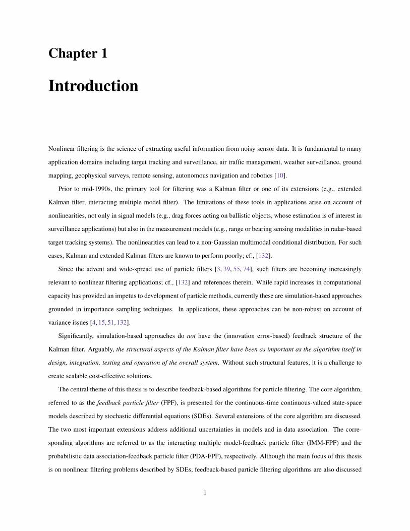
Nonlinear filtering is the science of extracting useful information from noisy sensor data. It is fundamental to many
application domains including target tracking and surveillance, air traffic management, weather surveillance, ground
mapping, geophysical surveys, remote sensing, autonomous navigation and robotics [10].
Prior to mid-1990s, the primary tool for filtering was a Kalman filter or one of its extensions (e.g., extended
Kalman filter, interacting multiple model filter). The limitations of these tools in applications arise on account of
nonlinearities, not only in signal models (e.g., drag forces acting on ballistic objects, whose estimation is of interest in
surveillance applications) but also in the measurement models (e.g., range or bearing sensing modalities in radar-based
target tracking systems). The nonlinearities can lead to a non-Gaussian multimodal conditional distribution. For such
cases, Kalman and extended Kalman filters are known to perform poorly; cf., [132].
Since the advent and wide-spread use of particle filters [3, 39, 55, 74], such filters are becoming increasingly
relevant to nonlinear filtering applications; cf., [132] and references therein. While rapid increases in computational
capacity has provided an impetus to development of particle methods, currently these are simulation-based approaches
grounded in importance sampling techniques. In applications, these approaches can be non-robust on account of
variance issues [4, 15, 51, 132].
Significantly, simulation-based approaches do not have the (innovation error-based) feedback structure of the
Kalman filter. Arguably, the structural aspects of the Kalman filter have been as important as the algorithm itself in
design, integration, testing and operation of the overall system. Without such structural features, it is a challenge to
create scalable cost-effective solutions.
The central theme of this thesis is to describe feedback-based algorithms for particle filtering. The core algorithm,
referred to as the feedback particle filter (FPF), is presented for the continuous-time continuous-valued state-space
models described by stochastic differential equations (SDEs). Several extensions of the core algorithm are discussed.
The two most important extensions address additional uncertainties in models and in data association. The corre-
sponding algorithms are referred to as the interacting multiple model-feedback particle filter (IMM-FPF) and the
probabilistic data association-feedback particle filter (PDA-FPF), respectively. Although the main focus of this thesis
is on nonlinear filtering problems described by SDEs, feedback-based particle filtering algorithms are also discussed
1
for continuous-time Markov chain models and for certain discrete-time models.
The organization of the remainder of this chapter is as follows. Sec. 1.1 presents the mathematical problem of
nonlinear filtering considered in this thesis along with an enumerated list of its applications. Sec. 1.2 summarizes the
classic Kalman filter as well as the conventional particle filter algorithm. Sec. 1.3 presents the feedback-control based
architecture for filtering together with a discussion of relevant prior literature. Sec. 1.4 and Sec. 1.5 describes the main
contributions and the layout of this thesis, respectively.
1.1 Problem Statement
Consider the filtering problem:
dXt = a(Xt)dt +σ(Xt)dBt , (1.1a)
dZt = h(Xt)dt + dWt , (1.1b)
where Xt ∈ Rd is the state (signal), Zt ∈ Rm is the observation (measurement), a(·), h(·) are C1 functions, and Bt,
Wt are mutually independent standard Wiener processes of appropriate dimension. Unless otherwise noted, the
SDEs in this thesis are expressed in Ito form.
The objective of the filtering problem is to compute the posterior distribution of Xt given the filtration (history of
observations) Zt := σ(Zs : s≤ t). The posterior p∗ is defined so that, for any measurable set A⊂ Rd ,
∫x∈A
p∗(x, t) dx = PXt ∈ A |Zt. (1.2)
The theory of general nonlinear filtering is described in the classic monograph [91]. The evolution of the posterior p∗
is described by the Kushner-Stratonovich (K-S) equation [100, 135]:
dp∗ = L † p∗ dt +(h− h)T (dZt − hdt)p∗, (1.3)
where h =∫
h(x)p∗(x, t)dx and L † p∗ =−∇ · (p∗a)+ 12 ∑
dl,k=1
∂ 2
∂xl∂xk
(p∗[σσT ]lk
).
The filter (1.3) is infinite-dimensional since it defines the evolution, in the space of probability measures, of
p∗( · , t) : t ≥ 0. Under few circumstances, (1.3) reduces to a finite-dimensional filter. If a( ·), h( ·) are linear
functions, the solution is given by the finite-dimensional Kalman-Bucy filter [34, 92]. If the underlying state evolves
as a continuous-time Markov chain, the solution is given by the Wonham filter [148]. Another example of the finite-
dimensional filter is the Benes filter [12]. For infinite-dimensional filter, numerical methods are used to approximate
2

the nonlinear filter (1.3) (see survey [36]).
In nonlinear filtering, there are two major problems of research interest:
(i) Numerical methods for solving the nonlinear filtering problem (1.3). This involves numerical approximation of
the posterior distribution p∗, which is typically an infinite-dimensional object. Several class of numerical methods
have been developed for this purpose, such as the projection filter/moment methods [31], spectral methods [109],
PDE methods [38] and the particle methods (also known as particle filters or sequential Monte Carlo methods) [74].
Although successfully applied to a variety of settings, particle filters often yield high variance, suffer particle de-
generacy and are known to be unstable even in low-order models [13]. Therefore it is essential to come up with new
computational methods which overcome these difficulties.
(ii) Algorithms for nonlinear filtering in the presence of model and data association uncertainties. It has been
recognized that there can be additional uncertainties associated with the filtering problem in addition to pro-
cess/observation noise. In applications involving tracking a maneuvering target, the target’s dynamic model can
randomly switch from one to another. In multiple target tracking applications, the measurement-to-target relation-
ship is not apriori known in a cluttered environment. Nonlinear filtering algorithms that can handle such uncertain-
ties are therefore of significant practical importance.
This thesis is devoted to solving these two problems stated above. For the first problem, a new framework for non-
linear filtering is proposed based on ideas from optimal control and mean-field game theory. The proposed feedback
particle filter admits an innovation-error based feedback control structure and requires no importance sampling or re-
sampling. For the second problem, the filter is generalized for problems involving additional uncertainties, including
model uncertainty and data association uncertainty. The feedback control structure is shown to be preserved for both
cases, even for the nonlinear non-Gaussian setting. Details on these topics appear in the following chapters.
1.1.1 Applications
Before proceeding to the next section, it is useful to list some practical applications of nonlinear filtering. The list is
far from exhaustive and it serves mainly to show the wide usage and impact of filtering.
1. Navigation and target tracking: One classic application of filtering is to navigate an object through unknown
terrain by estimating its current position based on sensor measurements [6, 35, 40, 77, 132]. Well-known ap-
plications include tracking and navigation of the Apollo spacecraft and the Mars orbiter. In recent years, the
wide-spread use of new sensors based on infrared, laser and other technologies requires novel approaches to
data fusion and tracking. More complicated applications also arise in problems with additional uncertainties,
3
such as model uncertainty (maneuvering target tracking) [10,21,112], and data association uncertainty (multiple
target tracking) [5,8,73]. Although the primary tool for tracking and navigation is a Kalman filter or an extended
Kalman filter, particle filters are becoming increasingly relevant to this field [28, 80, 101, 121, 151, 153].
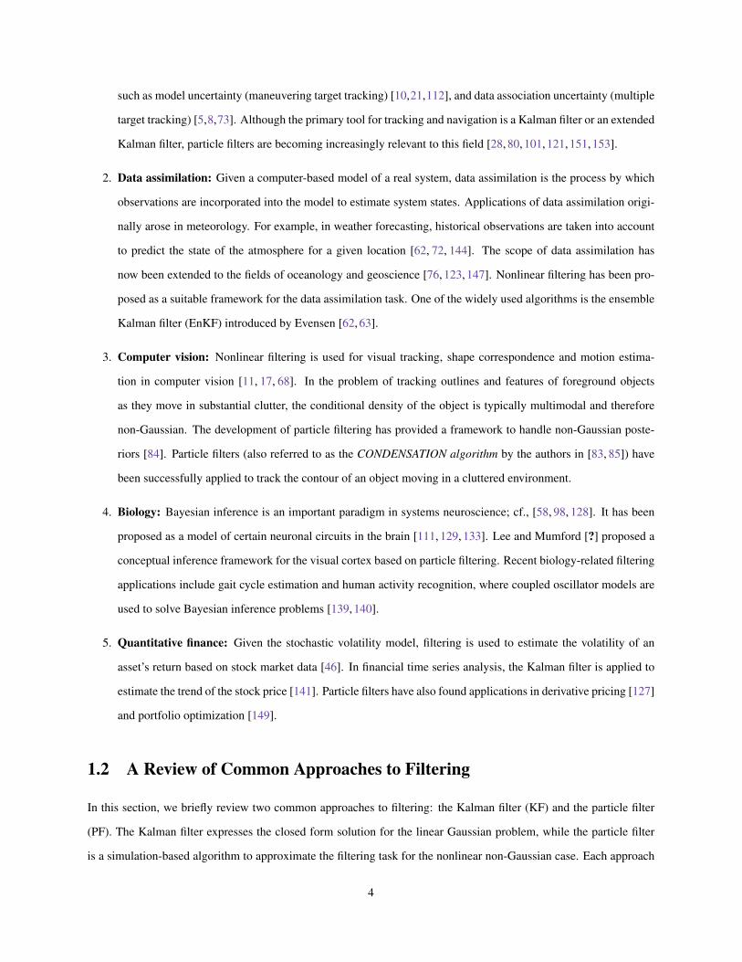
2. Data assimilation: Given a computer-based model of a real system, data assimilation is the process by which
observations are incorporated into the model to estimate system states. Applications of data assimilation origi-
nally arose in meteorology. For example, in weather forecasting, historical observations are taken into account
to predict the state of the atmosphere for a given location [62, 72, 144]. The scope of data assimilation has
now been extended to the fields of oceanology and geoscience [76, 123, 147]. Nonlinear filtering has been pro-
posed as a suitable framework for the data assimilation task. One of the widely used algorithms is the ensemble
Kalman filter (EnKF) introduced by Evensen [62, 63].
3. Computer vision: Nonlinear filtering is used for visual tracking, shape correspondence and motion estima-
tion in computer vision [11, 17, 68]. In the problem of tracking outlines and features of foreground objects
as they move in substantial clutter, the conditional density of the object is typically multimodal and therefore
non-Gaussian. The development of particle filtering has provided a framework to handle non-Gaussian poste-
riors [84]. Particle filters (also referred to as the CONDENSATION algorithm by the authors in [83, 85]) have
been successfully applied to track the contour of an object moving in a cluttered environment.
4. Biology: Bayesian inference is an important paradigm in systems neuroscience; cf., [58, 98, 128]. It has been
proposed as a model of certain neuronal circuits in the brain [111, 129, 133]. Lee and Mumford [?] proposed a
conceptual inference framework for the visual cortex based on particle filtering. Recent biology-related filtering
applications include gait cycle estimation and human activity recognition, where coupled oscillator models are
used to solve Bayesian inference problems [139, 140].
5. Quantitative finance: Given the stochastic volatility model, filtering is used to estimate the volatility of an
asset’s return based on stock market data [46]. In financial time series analysis, the Kalman filter is applied to
estimate the trend of the stock price [141]. Particle filters have also found applications in derivative pricing [127]
and portfolio optimization [149].
1.2 A Review of Common Approaches to Filtering
In this section, we briefly review two common approaches to filtering: the Kalman filter (KF) and the particle filter
(PF). The Kalman filter expresses the closed form solution for the linear Gaussian problem, while the particle filter
is a simulation-based algorithm to approximate the filtering task for the nonlinear non-Gaussian case. Each approach
4
-+
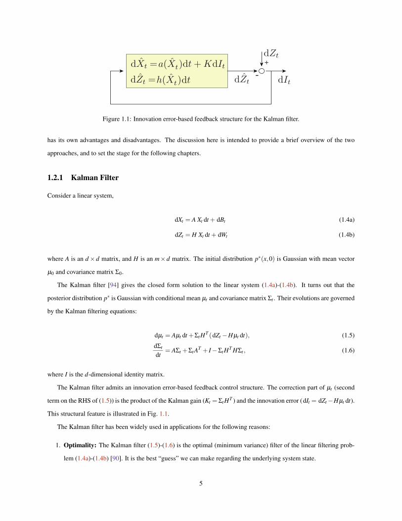
Figure 1.1: Innovation error-based feedback structure for the Kalman filter.
has its own advantages and disadvantages. The discussion here is intended to provide a brief overview of the two
approaches, and to set the stage for the following chapters.
1.2.1 Kalman Filter
Consider a linear system,
dXt = A Xt dt + dBt (1.4a)
dZt = H Xt dt + dWt (1.4b)
where A is an d× d matrix, and H is an m× d matrix. The initial distribution p∗(x,0) is Gaussian with mean vector
µ0 and covariance matrix Σ0.
The Kalman filter [94] gives the closed form solution to the linear system (1.4a)-(1.4b). It turns out that the
posterior distribution p∗ is Gaussian with conditional mean µt and covariance matrix Σt . Their evolutions are governed
by the Kalman filtering equations:
dµt = Aµt dt +ΣtHT (dZt −Hµt dt), (1.5)
dΣt
dt= AΣt +ΣtAT + I−ΣtHT HΣt , (1.6)
where I is the d-dimensional identity matrix.
The Kalman filter admits an innovation error-based feedback control structure. The correction part of µt (second
term on the RHS of (1.5)) is the product of the Kalman gain (Kt = ΣtHT ) and the innovation error (dIt = dZt−Hµt dt).
This structural feature is illustrated in Fig. 1.1.
The Kalman filter has been widely used in applications for the following reasons:
1. Optimality: The Kalman filter (1.5)-(1.6) is the optimal (minimum variance) filter of the linear filtering prob-
lem (1.4a)-(1.4b) [90]. It is the best “guess” we can make regarding the underlying system state.
5

2. Robustness: The Kalman filter is guaranteed to be stable under very mild conditions (e.g., controllability and
observability of the system model) [93]. The feedback control structure of the Kalman filter makes it robust to
a certain degree of uncertainty inherent in any model [158].
3. Cost efficiency: Only the conditional mean and covariance matrix are propagated at each time step (see (1.5)-
(1.6)). Therefore it is much more efficient compared to sampling-based algorithms, where the entire distribution
is propagated through particles [57, 158].
4. Ease of design, testing and operation: On account of the structural features, Kalman filter-based solutions
can be easily extended to other problems, such as the probabilistic data association filter for the data asso-
ciation problem [8], and the interacting multiple model filter for the estimation problem of stochastic hybrid
systems [21]. The separate treatment for the gain function and the innovation error is also helpful for debugging
and testing of large-scale problems [158].
The biggest limitation of the Kalman filter is the linear Gaussian assumption. For nonlinear systems in particular,
the Kalman filter is known to perform poorly; cf., [132]. One remedy is the extended Kalman filter (EKF), which
uses the linearized model in the update equations [1]. Other KF-based approaches for nonlinear filtering include the
unscented Kalman filter (UKF) [146], ensemble Kalman filter (EnKF) [62]. Nevertheless, in all these approaches, the
performance deteriorates as the nonlinearity becomes severe [89]. This motivates the study of sampling-based particle
filter algorithms.
1.2.2 Particle Filter
For nonlinear systems, the particle filter is a simulation-based algorithm to approximate the filtering task (1.1a)-(1.1b)
(see survey articles [36, 55, 74, 78]). The key step is the construction of N stochastic processes X it : 1 ≤ i ≤ N.
The value X it ∈ Rd is the state for the ith particle at time t. For each time t, the empirical distribution formed by, the
“particle population” is used to approximate the conditional distribution. It is defined for any measurable set A⊂ Rd
by,
p(N)(A, t) =1N
N
∑i=1
1lX it ∈ A. (1.7)
A common approach in particle filtering is called sequential importance resampling (SIR), where particles are
generated according to their importance weight at every time stage [36, 55]. By choosing the sampling mechanism
properly, particle filtering can approximately propagate the posterior distribution, with the accuracy improving as N
increases [44].
We sketch the implementation for the SIR particle filter (also known as the bootstrap particle filter), which is based
on an algorithm taken from Chap. 9 of [7]. The Euler discretization is used and the resulting discrete-time algorithm
6
is as follows: Consider the evolution of the ensemble
(X it ,w
it)−→ (X i
t+δ,wi
t+δ),
as new observations are obtained; here δ is the time-step and wit is the importance weight of the ith particle at time t.
This evolution is carried out in three steps [138]:
1. Prediction: Prediction involves using the SDE model (1.1a) to push-forward the particles, X it −→ X i−
t+δ. This is
accomplished by numerically integrating the SDE using Euler method. The weights wi−t+δ
= wit .
At the end of prediction step, the particles are denoted as (X i−t+δ
,wi−t+δ
).
2. Update: The update step involves application of the Bayes’ formula to update the weights. Given a new observation,
Zt+δ , the unnormalized weights are obtained as,
wi−t+δ
= wi−t+δ
L(δZ|X i−t+δ
), (1.8)
where δZ := Zt+δ −Zt and L(δZ|X i−t+δ
) := (2π)−m2 δ−
12 exp
[− ‖δZ−h(X i−
t+δ)δ‖2
2δ
]. The weights at time t + δ are then
obtained by normalization,
wit+δ
=wi−
t+δ
∑Nj=1 w j−
t+δ
. (1.9)
3. Resampling: The resampling step involves sampling X it+δ
with replacement from the set of particle positions
X i−t+δN
i=1 according to the probability vector of normalized weights wit+δN
i=1. After resampling, the particles are
set to be equally-weighted for the next iteration: wit+δ
= 1N . The resampling step is required in SIR particle filter
because of the issue of particle degeneracy, whereby only a few particles have insignificant weight values. Other pop-
ular methods for resampling are surveyed in [4], including systematic resampling, stratified resampling and residual
resampling.
The SIR particle filter approximates the true posterior p∗ by the empirical measure p(N) defined in (1.7). The
expectation of any test function φ : Rd → R given by
I(φ) :=∫
φ(x)p∗(x)dx,
is thus estimated by:
I(φ) :=∫
φ(x)p(N)(x)dx =1N
N
∑i=1
φ(X it ), (1.10)
Its straightforward to check that the SIR estimator (1.10) is unbiased and consistent. The variance of this estimator is
7

defined as
VarSIR[I(φ)
]:= E
[(I(φ)− I(φ))2] . (1.11)
The particle filter algorithm, as opposed to the linear Kalman filter, is applicable to a general class of nonlinear
non-Gaussian problems. However, this sampling-based approach suffers from several notable drawbacks:
1. Particle degeneracy: It refers to the case where after a few (even one) observations, nearly all particles have
zero weight values (one particle has unity weight). With a reduced effective sampling size, large computational
effort is devoted to updating particles whose contribution is almost zero. It has been shown that the degeneracy
phenomenon is impossible to avoid in importance sampling [56]. The root cause for particle degeneracy is the
point-by-point multiplication implementation of Bayes’ rule; cf., [13, 52, 57]. Common remedy is to occasion-
ally “rejuvenate” the particle population via resampling: i.e., eliminate particles that have small weights and
reproduce particles that have larger weights.
2. Sample impoverishment: Although resampling can potentially alleviate particle degeneracy, the benefit comes
at the cost of reducing the quality of the path-space representation [4, 57]. This is because after resampling, the
particles that have high weights wit are statistically selected many times. This leads to a loss of diversity among
the particles as the resultant sample will contain many repeated points. This problem, which is known as sample
impoverishment, is severe in the case of small process noise.
3. Curse of dimensionality: As a result of particle degeneracy, the number of particles required to achieve a
certain accuracy grows exponentially with the dimensionality of the state space [37, 47]. It is a fundamental
problem with the importance sampling-based particle filter. As expected, when applied to geophysical models
of high dimension, the classic particle filter is known to behave poorly after a few (or even one!) observation
cycles [2, 143].
4. Computational cost: The importance sampling step (requires point-by-point multiplication) and the resampling
step (requires the entire particle population) incurs high computational burden [53]. Resampling also limits the
opportunity for parallel computation since all the particles must be combined [4].
5. Variance: A issue common to sampling-based particle filters is the high variance of the resulting estima-
tor (1.10) [56, 70]. Under certain conditions, it is shown in [57] that the variance of the estimator defined
in (1.11) satisfies:
VarSIR[I(φ)
]≤ D
N,
where the constant D typically increases exponentially with the dimension of the state-space of Xt . The root
8

cause is the particle degeneracy which causes highly varying importance weights [13]. The variance of the
particle filter estimator can only be expected to be reasonable if the variance of the sample weights is small.
6. Numerical instability: The particle filter implementation is generally fragile for unstable systems, in contrast
to the Kalman filter, which is guaranteed to be stable under very mild conditions [51]. When the signal pro-
cess (1.1a) is unstable, individual particle can exhibit numerical instabilities due to time-discretization, floating
point representation, etc [158]. Recent efforts to understand the lack of stability for particle filters for unstable
systems are surveyed by Ramon van Handel in [142].
7. Difficulty in design, test and implementation: The innovation error in the Kushner’s equation (and in the
Kalman filter) does not appear explicitly in the sampling-based particle filters. Without such a feedback control
structure, it is a challenge to create scalable cost-effective solutions [158]: the optimal proposal density for
importance sampling is difficult to design [56]; and the choice of resampling step is often ad-hoc [57].
Readers are referred to [4, 57] for more details on both the theory and implementation of the convectional particle
filter.
1.3 Control-Oriented Particle Filtering
The objective of this work is to introduce an alternative approach to the construction of a particle filter for (1.1a)-
(1.1b) inspired by mean-field optimal control techniques; cf., [79, 160]. In this approach, the model for the ith particle
is defined by a controlled system,
dX it = a(X i
t )dt +σ(X it )dBi
t + dU it , (1.12)
where X it ∈ Rd is the state for the ith particle at time t, U i
t is its control input, and Bit are mutually independent
standard Wiener processes. Certain additional assumptions are made regarding admissible forms of the control input.
Throughout the thesis we denote conditional distribution of a particle X it given Zt by p, where for any measurable
set A⊂ Rd , ∫x∈A
p(x, t) dx = PX it ∈ A |Zt. (1.13)
Recall the actual posterior of the system state Xt is denoted as p∗ (defined in (1.2)). The initial conditions X i0N
i=1 are
assumed to be i.i.d., and drawn from initial distribution p∗(x,0) of X0 (i.e., p(x,0) = p∗(x,0)).
The control problem is to choose the control input U it so that p approximates p∗, and consequently p(N) (defined
in (1.7)) approximates p∗ for large N. The synthesis of the control input is cast as a variational problem, with the
Kullback-Leibler metric serving as the cost function. The optimal control input is obtained via analysis of the first
9
variation. The main objective is to derive an explicit formula for the optimal control input, and demonstrate that under
general conditions we obtain an exact match: p = p∗ under optimal control. Details for the proposed filter appear in
the following chapters.
1.3.1 Related Work
In recent years, there has been a burgeoning interest in application of ideas and techniques from statistical mechanics
to nonlinear estimation and control theory. Although some of these applications are classic (see e.g., Del Moral [54]),
the recent impetus comes from explosive interest in mean-field games, starting with two papers from 2007: Lasry and
Lions’ paper titled “Mean-field games” [103] and a paper by Huang, Caines and Malhame [79]. These papers spurred
interest in analysis and synthesis of controlled interacting particle systems.
The nonlinear estimation problem is a (mathematical) dual to the mean-field game control problem. Over the
years, Mitter has a number of publications on duality between estimation and control [30,67,116–118]. Mitter’s 2003
SIAM paper explicitly focused on a variational formulation of the nonlinear filtering problem with the objective of
constructing a particle filtering algorithm based on duality considerations [117]. The variational construction in [117]
was inspired by the variational formulation of the Fokker-Planck equation in the paper by Otto and collaborators [88].
The feedback particle filter algorithm (our approach) is a solution to the variational filtering problem (see also [104]).
Given the variational underpinnings, there are also close parallels with the optimal transportation theory [61,145]. For
image processing applications, this theory has been used extensively by Tannenbaum and collaborators [96,102,115].
Apart from our work, there have also been a number of papers on control-oriented approaches to particle filtering:
For the continuous-time filtering problem, an approximate particle filtering algorithm appears in the 2009 paper of
Crisan and Xiong [45]. In the 2003 paper of Mitter, an optimal control problem for particle filtering is formulated
based on duality [117]. Certain mean-field game inspired approximate algorithms for nonlinear estimation appear
in the recent papers by other groups [64, 65, 125]. In discrete-time settings, Daum and Huang have introduced the
particle flow algorithm [48–51]. A comparison of our work to Daum’s particle flow filter appears in [152]. Despite
the similarity, important differences exist between our approach and theirs, which are clarified in later chapters.
The innovative control structure in particle filtering is shown to be beneficial in terms of filter performance, ro-
bustness, stability as well as computational cost. There are by now a growing list of papers on application of such
controlled algorithms to: physical activity recognition [139, 140], estimation of soil parameters in dredging applica-
tions [134], estimation and control in the presence of communication channels [110], target state estimation [138],
weather forecasting [130].
10

(a) Kalman filter (b) Feedback Particle Filter
-+
-+
Figure 1.2: Innovation error-based feedback structure for (a) the Kalman filter and (b) the feedback particle filter.
1.4 Main Contributions of the Thesis
As discussed in Sec. 1.1, there are two major problems of research interest in nonlinear filtering: 1) Numerical methods
for solving the nonlinear filtering problem (1.3), and 2) Algorithms for nonlinear filtering in the presence of model
and data association uncertainties. Both subjects are studied in this thesis. The original contributions are as follows:
1. Feedback particle filter (FPF) algorithm: The proposed filter is defined by an ensemble of controlled particle
systems. Each particle evolves under feedback control based on its own state, and features of the empirical
distribution of the ensemble. The feedback control law in (1.12) is obtained as the solution to a variational
problem, where the optimization criterion is the Kullback-Leibler divergence between the actual posterior, and
the common posterior of any particle. The optimal control solution is shown to be exact in the sense that the
two posteriors match exactly, provided they are initialized with identical priors. The optimal filter admits an
innovation error-based feedback structure, and the optimal feedback gain is obtained via a solution of an Euler-
Lagrange boundary value problem (E-L BVP). See Fig. 1.2 for an illustration of the feedback control structure.
The feedback gain equals the Kalman gain in the linear Gaussian case. For the nonlinear case, the Kalman gain
is replaced by a nonlinear function of the state. These results have been published in [156–158].
2. Existence and uniqueness of FPF: Consistency is established in the general multivariate setting, as well as the
well-posedness of the associated BVP to obtain the filter gain function. The admissibility of the control input
in (1.12) is proved as a corollary. These results have been published in [154].
3. Numerical algorithms for gain function approximation: Several approaches have been proposed to solve
the BVP, including the direct numerical approximation, constant gain approximation and the Gaussian mixture
approximation. Motivated by a weak formulation of the BVP, a Galerkin finite-element algorithm has been
proposed to approximate the gain function. These results have been published in [154, 156].
4. FPF for discrete-time observation: The FPF algorithm is introduced for the continuous-discrete time non-
linear filtering problem. A continuous-discrete time analogue of the feedback control structure is derived.
Comparisons to existing continuous-discrete time algorithms, specifically the particle flow filter by Daum and
Huang [51], are also provided. These results have been published in [152].
11
5. FPF for a continuous-time Markov chain: The Wonham filter is shown to be approximated by the FPF
algorithm for the problem of estimating a continuous-time Markov chain. A complete characterization of the
feedback mechanism that defines the FPF is obtained, which leads to tractable algorithms for the nonlinear
filtering problem, even for large state space. These results have been published in [159].
The second half of this thesis focuses on the algorithms for nonlinear filtering with additional uncertainties in
models and in data association. Contributions are as follows:
6. Interacting Multiple Model-Feedback Particle Filter (IMM-FPF): The IMM-FPF is an algorithm for nonlin-
ear filtering in the presence of model uncertainty. The uncertainty is modeled using a stochastic hybrid system
(SHS) framework. The proposed filter is shown to be the nonlinear generalization of the classic Kalman filter-
based IMM filter. The theoretical results are illustrated with numerical examples for tracking a maneuvering
target. These results have been published in [151].
7. Probabilistic Data Association-Feedback Particle Filter (PDA-FPF): The PDA-FPF is an approximating
algorithm for nonlinear filtering in the presence of data association uncertainty. The proposed filter is shown
to represent a generalization - to the nonlinear non-Gaussian case - of the classic Kalman filter-based PDA
filter (PDAF). Numerical examples motivated by multiple target tracking applications are used to illustrate the
PDA-FPF. These results have been published in [153, 155].
One remarkable conclusion is that both the IMM-FPF and PDA-FPF retain the innovation error-based feedback struc-
ture as in the FPF, even for the nonlinear non-Gaussian case.
1.5 Layout of the Thesis
The remainder of the thesis is comprised of two parts. Part I covers the theory of the feedback particle filter: Chap. 2
contains an introduction to the fundamentals of the feedback particle filter. For pedagogical purpose, only the simplest
scalar case is presented. The multivariable feedback particle filter appears in Chap. 3, where well-posedness results are
also derived. The continuous-discrete time FPF algorithm is developed in Chap. 4, while the FPF for a continuous-time
Markov chain is discussed in Chap. 5.
Part II of this thesis concerns two applications of the feedback particle filter in the presence of additional uncertain-
ties. Specifically, Chap. 6 develops the IMM-FPF algorithm for the estimation problem of stochastic hybrid systems,
where model uncertainty is present. To deal with data association uncertainty, Chap. 7 first proposes the PDA-FPF
algorithm for the problem of tracking a single target in the presence of clutter. The JPDA-FPF for multiple target
tracking case follows as a straightforward extension. All proofs are summarized in appendices.
12
Part I
Feedback Particle Filter
13

Chapter 2
Fundamentals of the Feedback ParticleFilter∗
2.1 Introduction
In this chapter, the basic feedback particle filter is introduced for the continuous-time continuous-valued state-space
nonlinear filtering problem. The scalar case is described for pedagogical purposes and for ease of presentation. The
general multivariable case appears in Chap. 3.
The scalar filtering problem is modeled using stochastic differential equations (SDEs):
dXt = a(Xt)dt +σB dBt , (2.1a)
dZt = h(Xt)dt +σW dWt , (2.1b)
where Xt ∈R is the state at time t, Zt ∈R is the observation, a( ·), h( ·) are C1 functions, and Bt, Wt are mutually
independent standard Wiener processes. Unless otherwise noted, SDEs are expressed in Ito form.
The objective of the filtering problem is to compute or approximate the posterior distribution of Xt given the history
Zt := σ(Zs : s≤ t). The posterior p∗ is defined so that, for any measurable set A⊂ R,
∫x∈A
p∗(x, t) dx = PXt ∈ A |Zt. (2.2)
The feedback particle filter is an alternative approach to the construction of a particle filter for (2.1a)-(2.1b) inspired
by mean-field optimal control techniques; cf., [79, 160]. In this approach, the model for the ith particle is defined by a
controlled system,
dX it = a(X i
t )dt +σB dBit + dU i
t , (2.3)
where X it ∈ R is the state for the ith particle at time t, U i
t is its control input, and Bit are mutually independent
standard Wiener processes. Certain additional assumptions are made regarding admissible forms of control input.∗This chapter is an extension of the published paper [158].
14
We denote the conditional distribution of a particle X it given Zt by p where:
∫x∈A
p(x, t) dx = PX it ∈ A |Zt. (2.4)
The initial conditions X i0N
i=1 are assumed to be i.i.d., and drawn from initial distribution p∗(x,0) of X0 (i.e., p(x,0) =
p∗(x,0)).
The control problem is to choose the control input U it so that p approximates p∗, and consequently p(N) (the
empirical distribution formed by the “particle population”, as defined in (1.7)) approximates p∗ for large N. The
synthesis of the control input is cast as a variational problem, with the Kullback-Leibler metric serving as the cost
function. The optimal control input is obtained via analysis of the first variation.
The main result of this chapter is to derive an explicit formula for the optimal control input, and demonstrate that
under general conditions we obtain an exact match: p = p∗ under optimal control. The optimally controlled dynamics
of the ith particle have the following Ito form,
dX it = a(X i
t )dt +σB dBit +K(X i
t , t)dIit +Ω(X i
t , t)dt︸ ︷︷ ︸optimal control, dU i∗
t
, (2.5)
in which Iit is a certain modified form of the innovation process that appears in the nonlinear filter,
dIit := dZt −
12(h(X i
t )+ ht)
dt, (2.6)
where ht := E[h(X it )|Zt ] =
∫h(x)p(x, t)dx. In a numerical implementation, we approximate
ht ≈ h(N)t :=
1N
N
∑i=1
h(X it ) . (2.7)
The gain function K is shown to be the solution to the following Euler-Lagrange boundary value problem (E-L
BVP):∂
∂x(pK) =− 1
σ2W(h− ht)p, (2.8)
with boundary conditions limx→±∞ p(x, t)K(x, t) = 0, where h′(x) = ddx h(x). Note that the gain function needs to be
obtained for each value of time t.
Finally, Ω(x, t) is the Wong-Zakai correction term where Ω(x, t) := 12 σ2
W K(x, t)K′(x, t) and K′(x, t) = ∂K∂x (x, t). The
controlled system (2.5)-(2.8) is called the feedback particle filter.
The contributions of this chapter are as follows:
• Variational Problem. The construction of the feedback particle filter is based on a variational problem, where the
15

cost function is the Kullback-Leibler (K-L) divergence between p∗(x, t) and p(x, t). The feedback particle filter (2.5)-
(2.8), including the formula (2.6) for the innovation error and the E-L BVP (2.8), is obtained via analysis of the first
variation.
• Consistency. The particle filter model (2.5) is consistent with nonlinear filter in the following sense: Suppose the
gain function K(x, t) is obtained as the solution to (2.8), and the priors are consistent, p(x,0) = p∗(x,0). Then, for all
t ≥ 0 and all x,
p(x, t) = p∗(x, t).
• Algorithms. Numerical techniques are proposed for synthesis of the gain function K(x, t). If a(·) and h(·) are linear
and the density p∗ is Gaussian, then the gain function is simply the Kalman gain. At time t, it is a constant given in
terms of variance alone. The variance is approximated empirically as a sample covariance.
In the nonlinear case, numerical approximation techniques are described. A Galerkin finite-element algorithm
appears in Chap. 3. Another approach based on the Gaussian mixture approximation is discussed in [156].
In recent decades, there have been many important advances in importance sampling based approaches for particle
filtering; cf., [36,55,150]. A crucial distinction here is that there is no importance sampling or resampling of particles.
We believe that the introduction of control in the feedback particle filter has several useful features/advantages:
Does not require sampling. There is no importance sampling or resampling required as in the conventional particle
filter. This property allows the feedback particle filter to be flexible with regards to implementation and does not suffer
from sampling-related issues, such as particle degeneracy or sample impoverishment.
Innovation error. The innovation error-based feedback structure is a key feature of the feedback particle filter (2.5).
The innovation error in (2.5) is based on the average value of the prediction h(X it ) of the ith-particle and the prediction
ht due to the entire population.
The feedback structure is easier to see when the filter is expressed in its Stratonovich form:
dX it = a(X i
t )dt + dBit +K(X i, t)
(dZt −
12(h(X i
t )+ ht)dt). (2.9)
Given that the Stratonovich form provides a mathematical interpretation of the (formal) ODE model [122, Section
3.3], we also obtain the ODE model of the filter. Denoting Yt.= dZt
dt and white noise process Bit.= dBi
tdt , the ODE model
of the filter is given by,dX i
t
dt= a(X i
t )+ Bit +K(X i, t) ·
(Yt −
12(h(X i
t )+ ht)
).
The “innovation” of the feedback particle filter thus lies in the (modified) definition of innovation error for a
particle filter (see (2.6)). Moreover, the feedback control structure that existed thusfar only for the Kalman filter now
16

Figure 2.1: Innovation error-based feedback structure for (a) the Kalman filter and (b) the feedback particle filter (inODE model).
also exists for particle filters (compare parts (a) and (b) of Fig. 2.1). For the linear case, the optimal gain function is
the Kalman gain. For the nonlinear case, the Kalman gain is replaced by a nonlinear function of the state.
Feedback structure. Feedback is important on account of the issue of robustness. A filter is based on an idealized
model of the underlying dynamic process that is often nonlinear, uncertain and time-varying. The self-correcting
property of the feedback provides robustness, allowing one to tolerate a degree of uncertainty inherent in any model.
In contrast, a conventional particle filter is based upon importance sampling. Although the innovation error is
central to the Kushner-Stratonovich’s stochastic partial differential equation (SPDE) of nonlinear filtering, it is con-
spicuous by its absence in a conventional particle filter.
Arguably, the structural aspects of the Kalman filter have been as important as the algorithm itself in design,
integration, testing and operation of the overall system. Without such structural features, it is a challenge to create
scalable cost-effective solutions.
Variance reduction. Feedback can help reduce the high variance that is sometimes observed in the conventional
particle filter. Numerical results in Sec. 2.5 support this claim — See Fig. 2.3 for a comparison of the feedback
particle filter and the bootstrap particle filter.
Ease of design, testing and operation. On account of structural features, feedback particle filter-based solutions are
expected to be more robust, cost-effective, and easier to debug and implement.
Applications. Bayesian inference is an important paradigm used to model functions of certain neural circuits in the
brain [58, 105]. Compared to techniques that rely on importance sampling, a feedback particle filter may provide a
more neuro-biologically plausible model to implement filtering and inference functions. It is illustrated in this chapter
with the aid of a filtering problem involving nonlinear oscillators. Another application appears in [139, 140].
The remainder of this chapter is organized as follows: The variational setup is described in Sec. 2.2: It begins
with a discussion of the continuous-discrete filtering problem: the equation for dynamics is defined by (2.1a), but the
observations are made only at discrete times. The continuous-time filtering problem (for (2.1a)-(2.1b)) is obtained as
a limiting case of the continuous-discrete problem.
The feedback particle filter is introduced in Sec. 2.3. Algorithms are discussed in Sec. 2.4, and numerical examples
are described in Sec. 2.5, including the neuroscience application involving coupled oscillator models. These models
17

(also considered in our earlier mean-field control paper [160]) provided some of the initial motivation for the present
work.
2.2 Variational Problem
The precise formulation of the variational problem begins with the continuous time model, with sampled observations.
The equation for dynamics is given by (2.1a), and the observations are made only at discrete times tn:
Ytn = h(Xtn)+W4tn , (2.10)
where 4 := tn+1− tn and W4tn is i.i.d and drawn from N(0, σ2W4 ).
The particle model in this case is a hybrid dynamical system: For t ∈ [tn−1, tn), the ith particle evolves according
to the stochastic differential equation,
dX it = a(X i
t )dt +σB dBit , tn−1 ≤ t < tn , (2.11)
where the initial condition X itn−1
is given. At time t = tn there is a potential jump that is determined by the input U itn :
X itn = X i
t−n+U i
tn , (2.12)
where X it−n
denotes the right limit of X it : tn−1 ≤ t < tn. The specification (2.12) defines the initial condition for the
process on the next interval [tn, tn+1).
The filtering problem is to construct a control law that defines U itn : n≥ 1 such that p( · , tn) approximates p∗( · , tn)
for each n ≥ 1. To solve this problem we first define “belief maps” that propagate the conditional distributions of X t
and X it .
2.2.1 Belief Maps
The observation history is denoted Yn := σYtk : k ≤ n,k ∈ N. For each n, various conditional distributions are
considered:
1) p∗n and p∗−n : The conditional distribution of Xtn given Yn and Yn−1, respectively.
2) pn and p−n : The conditional distribution of X itn given Yn and Yn−1, respectively.
18
These densities evolve according to recursions of the form,
p∗n = P∗(p∗n−1,Ytn), pn = P(pn−1,Ytn) . (2.13)
The mappings P∗ and P can be decomposed into two parts. The first part is identical for each of these mappings:
the transformation that takes pn−1 to p−n coincides with the mapping from p∗n−1 to p∗−n . In each case it is defined by
the Kolmogorov forward equation associated with the diffusion on [tn−1, tn).
The second part of the mapping is the transformation that takes p∗−n to p∗n, which is obtained from Bayes’ rule:
Given the observation Ytn made at time t = tn,
p∗n(s) =p∗−n (s) · pY |X(Ytn |s)
pY(Ytn), s ∈ R, (2.14)
where pY denotes the pdf for Ytn , and pY |X( · | s) denotes the conditional distribution of Ytn given Xtn = s. Applying
(2.10) gives,
pY |X(Ytn | s) =1√
2πσ2W/4
exp(− (Ytn −h(s))2
2σ2W/4
).
Combining (2.14) with the forward equation defines P∗.
The transformation that takes p−n to pn depends upon the choice of control U itn in (2.12). At time t = tn, we seek a
control input U itn that is admissible.
Definition 1 (Admissible Input) The control sequence U itn : n ≥ 0 is admissible if there is a sequence of maps
vn(x;yn0) such that U i
tn = vn(X it−n,Yt0 , . . . ,Ytn) for each n, and moreover,
(i) E[|U itn |]< ∞, and with probability one,
limx→±∞
vn(x,Yt0 , . . . ,Ytn)p−n (x) = 0.
(ii) vn is twice continuously differentiable as a function of x.
(iii) 1+ v′n(x) is non-zero for all x, where v′n(x) =ddx vn(x).
We will suppress the dependency of vn on the observations (and often the time-index n), writing U itn = v(x) when
X it−n
= x. Under the assumption that 1+ v′(x) is non-zero for all x, we can write,
pn(x+) =p−n (x)|1+ v′(x)| , where x+ = x+ v(x). (2.15)
19

2.2.2 Variational Problem
Our goal is to choose an admissible input so that the mapping P approximates the mapping P∗ in (2.13). More
specifically, given the pdf pn−1 we have already defined the mapping P so that pn = P(pn−1,Ytn). We denote
p∗n = P∗(pn−1,Ytn), and choose vn so that these pdfs are as close as possible. We approach this goal through the
formulation of an optimization problem with respect to the KL divergence metric. That is, at time t = tn, the function
vn is the solution to the following optimization problem,
vn(x) = arg minv
D(pn‖p∗n) . (2.16)
Based on the definitions, for any v the KL divergence can be expressed,
D(pn‖p∗n) =−∫R
p−n (x)
ln |1+ v′(x)|+ ln(
p−n (x+ v(x))pY |X(Ytn |x+ v(x)))
dx+C, (2.17)
where C =∫R p−n (x) ln(p−n (x)pY(Ytn))dx is a constant that does not depend on v; cf., App. A.1 for the calculation.
The solution to (2.16) is described in the following proposition, whose proof appears in App. A.2.
Proposition 2.2.1 Suppose that the admissible input is obtained as the solution to the sequence of optimization prob-
lems (2.16). Then for each n, the function v = vn is a solution of the following Euler-Lagrange (E-L) BVP:
ddx
(p−n (x)|1+ v′(x)|
)= p−n (x)
∂
∂v
(ln(p−n (x+ v)pY |X(Ytn |x+ v))
), (2.18)
with boundary condition limx→±∞ v(x)p−n (x) = 0.
We refer to the minimizer as the optimal control function. Additional details on the continuous-discrete time filter
appear in our conference paper [157].
2.3 Feedback Particle Filter
We now consider the continuous time filtering problem (2.1a, 2.1b) introduced in Sec. 2.1.
2.3.1 Belief State Dynamics and Control Architecture
The model for the particle filter is given by the Ito diffusion,
dX it = a(X i
t )dt +σB dBit +u(X i
t , t)dt +K(X it , t)dZt︸ ︷︷ ︸
dU it
, (2.19)
20
where X it ∈ R is the state for the ith particle at time t, and Bi
t are mutually independent standard Wiener processes.
We assume the initial conditions X i0N
i=1 are i.i.d., independent of Bit, and drawn from the initial distribution p∗(x,0)
of X0. Both Bit and X i
0 are also assumed to be independent of Xt ,Zt .
As in Sec. 2.2, we impose admissibility requirements on the control input U it in (2.19):
Definition 2 (Admissible Input) The control input U it is admissible if the random variables u(x, t) and K(x, t) are
Zt = σ(Zs : s≤ t) measurable for each t. Moreover, each t,
(i) E[|u(X it , t)|+ |K(X i
t , t)|2]< ∞, and with probability one,
limx→±∞
u(x, t)p(x, t) = 0, (2.20a)
limx→±∞
K(x, t)p(x, t) = 0. (2.20b)
where p is the posterior distribution of X it given Zt , defined in (2.4).
(ii) u : R2→ R, K : R2→ R are twice continuously differentiable in their first arguments.
The functions u(x, t),K(x, t) represent the continuous-time counterparts of the optimal control function vn(x)
(see (2.16)). We say that these functions are optimal if p≡ p∗, where recall p∗ is the posterior distribution of Xt given
Zt as defined in (2.2). Given p∗(·,0) = p(·,0), our goal is to choose u,K in the feedback particle filter so that the
evolution equations of these conditional distributions coincide.
The evolution of p∗(x, t) is described by the Kushner-Stratonovich (K-S) equation:
dp∗ = L † p∗ dt +1
σ2W(h− ht)(dZt − ht dt)p∗, (2.21)
where ht =∫
h(x)p∗(x, t)dx, and L † p∗ =− ∂ (p∗a)∂x +
σ2B
2∂ 2 p∗∂x2 .
The evolution equation of p(x, t) is described next. The proof appears in App. A.3.
Proposition 2.3.1 Consider the process X it that evolves according to the particle filter model (2.19). The conditional
distribution of X it given the filtration Zt , p(x, t), satisfies the forward equation
dp = L † pdt− ∂
∂x(Kp) dZt −
∂
∂x(up) dt +σ
2W
12
∂ 2
∂x2
(pK2) dt. (2.22)
2.3.2 Consistency with the Nonlinear Filter
The main result of this section is the construction of an optimal pair u,K under the following assumption:
21
Assumption A1 The conditional distributions (p∗, p) are C2, with p∗(x, t)> 0 and p(x, t)> 0, for all x ∈ R, t > 0.
We henceforth choose u,K as the solution to a certain E-L BVP based on p: the function K is the solution to
∂
∂x(pK) =− 1
σ2W(h− ht)p, (2.23)
with boundary condition (2.20b). The function u(·, t) : R→ R is obtained as:
u(x, t) = K(x, t)(−1
2(h(x)+ ht)+
12
σ2W K′(x, t)
), (2.24)
where ht =∫
h(x)p(x, t)dx. We assume moreover that the control input obtained using u,K is admissible. The
particular form of u given in (2.24) and the BVP (2.23) is motivated by considering the continuous-time limit of (2.18),
obtained on letting 4 := tn+1− tn go to zero; the calculations appear in App. A.4.
Existence and uniqueness of u,K is obtained in the following proposition — Its proof is given in App. A.5.
Proposition 2.3.2 Consider the BVP (2.23), subject to Assumption A1. Then,
1) There exists a unique solution K, subject to the boundary condition (2.20b).
2) The solution satisfies K(x, t)≥ 0 for all x, t, provided h′(x)≥ 0 for all x.
The following theorem shows that the two evolution equations (2.21) and (2.22) are identical. The proof appears
in App. A.6.
Theorem 2.3.3 Consider the two evolution equations for p and p∗, defined according to the solution of the forward
equation (2.22) and the K-S equation (2.21), respectively. Suppose that the control functions u(x, t) and K(x, t) are
obtained according to (2.23) and (2.24), respectively. Then, provided p(x,0) = p∗(x,0), we have for all t ≥ 0,
p(x, t) = p∗(x, t)
Remark 1 Thm. 2.3.3 is based on the ideal setting in which the gain K(X it , t) is obtained as a function of the posterior
p = p∗ for X it . In practice the algorithm is applied with p replaced by the empirical distribution of the N particles.
In this ideal setting, the empirical distribution of the particle system will approximate the posterior distribution
p∗(x, t) as N→∞. The convergence is in the weak sense in general. To obtain almost sure convergence, it is necessary
to obtain sample path representations of the solution to the stochastic differential equation for each i (see e.g. [99]).
22

Under these conditions the solution to the SDE (2.3) for each i has a functional representation,
X it = F(X i
0,Bi[0,t];Z[0,t]),
where the notation Z[0,t] signifies the entire sample path Zs : 0≤ s≤ t for a stochastic process Z; F is a continuous
functional (in the uniform topology) of the sample paths Bi[0,t],Z[0,t] along with the initial condition X i
0. It follows
that the empirical distribution has a functional representation,
p(N)(A, t) =1N
N
∑i=1
1lF(X i0,B
i[0,t];Z[0,t]) ∈ A
The sequence (X i0,B
i[0,t]) : i = 1, ... is i.i.d. and independent of Z. It follows that the summand 1lF(X i
0,Bi[0,t];Z[0,t]) :
i = 1, . . . is also i.i.d. given Z[0,t]. Almost sure convergence follows from the Law of Large Numbers for scalar i.i.d.
sequences.
In current research we are considering the more difficult problem of performance bounds for the approximate
implementations described in Sec. 2.4.
Remark 2 Although the methodology and the filter is presented for Gaussian process and observation noise, the case
of non-Gaussian process noise is easily handled – simply replace the noise model in the filter with the appropriate
model of the process noise.
For other types of observation noise, one would modify the conditional distribution pY |X in the optimization prob-
lem (2.16). The derivation of filter would then proceed by consideration of the first variation (see App. A.4).
2.3.3 Example: Linear Model
It is helpful to consider the feedback particle filter in the following simple linear setting,
dXt = α Xt dt +σB dBt , (2.25a)
dZt = γ Xt dt +σW dWt , (2.25b)
where α , γ are real numbers. The initial distribution p∗(x,0) is assumed to be Gaussian with mean µ0 and variance
Σ0.
The following lemma provides the solution of the gain function K(x, t) in the linear Gaussian case.
Lemma 2.3.4 Consider the linear observation equation (2.25b). If p(x, t) is assumed to be Gaussian with mean µt
23
and variance Σt , then the solution of E-L BVP (2.8) is given by:
K(x, t) =Σtγ
σ2W. (2.26)
The formula (2.26) is verified by direct substitution in the ODE (2.8) where the distribution p is Gaussian.
The optimal control yields the following form for the particle filter in this linear Gaussian model:
dX it = α X i
t dt +σB dBit +
Σtγ
σ2W
(dZt − γ
X it +µt
2dt). (2.27)
Now we show that p = p∗ in this case. That is, the conditional distributions of X t and X it coincide, and are defined
by the well-known dynamic equations that characterize the mean and the variance of the continuous-time Kalman
filter. The proof appears in App. A.7.
Theorem 2.3.5 Consider the linear Gaussian filtering problem defined by the state-observation equations (2.25a,2.25b).
In this case the posterior distributions of X t and X it are Gaussian, whose conditional mean and covariance are given
by the respective SDE and the ODE,
dµt = αµt dt +Σtγ
σ2W
(dZt − γµt dt
)(2.28)
ddt
Σt = 2αΣt +σ2B−
(γ)2Σ2t
σ2W
(2.29)
Notice that the particle system (2.27) is not practical since it requires computation of the conditional mean and
variance µt ,Σt. If we are to compute these quantities, then there is no reason to run a particle filter!
In practice µt ,Σt are approximated as sample means and sample covariances from the ensemble X it N
i=1:
µt ≈ µ(N)t :=
1N
N
∑i=1
X it ,
Σt ≈ Σ(N)t :=
1N−1
N
∑i=1
(X i
t −µ(N)t
)2.
(2.30)
The resulting equation (2.27) for the ith particle is given by
dX it = α X i
t dt +σB dBit +
Σ(N)t γ
σ2W
(dZt − γ
X it +µ
(N)t
2dt
). (2.31)
It is very similar to the mean-field “synchronization-type” control laws and oblivious equilibria constructions as in
[79, 160]. The model (2.27) represents the mean-field approximation obtained by letting N→ ∞.
24
The control term in the linear feedback particle filter (2.30)-(2.31) appears also in the work of Reich [130], where
it is referred to as the ensemble square root filter.
2.4 Synthesis of the Gain Function
Implementation of the nonlinear filter (2.5) requires solution of the E-L BVP (2.8) to obtain the gain function K(x, t)
for each fixed t.
2.4.1 Direct Numerical Approximation of the BVP Solution
The explicit closed-form formula (A.15) for the solution of the BVP (2.8) can be used to construct a direct numerical
approximation of the solution. Using (A.15), we have
K(x, t) =1
p(x, t)1
σ2W
∫ x
−∞
(ht −h(y))p(y, t)dy.
The approximation involves three steps:
1) Approximation of ht by using a sample mean:
ht ≈1N
N
∑j=1
h(X jt ) =: h(N)
t .
2) Approximation of the integrand:
(ht −h(y))p(y, t)≈ 1N
N
∑j=1
(h(N)t −h(X j
t ))δ (y−X jt ),
where δ (·) is the Dirac delta function.
3) Approximation of the density p(x, t) in the denominator, e.g., as a sum of Gaussian:
p(x, t)≈ 1N
N
∑j=1
q jt (x) =: p(x, t), (2.32)
where q jt (x) = q(x;X j
t , ε) =1√2πε
exp(− 1
2ε (x−X jt )
2)
. The appropriate value of ε depends upon the problem. As a
function of N, ε can be made smaller as N grows; As N→ ∞, ε→ 0.
25
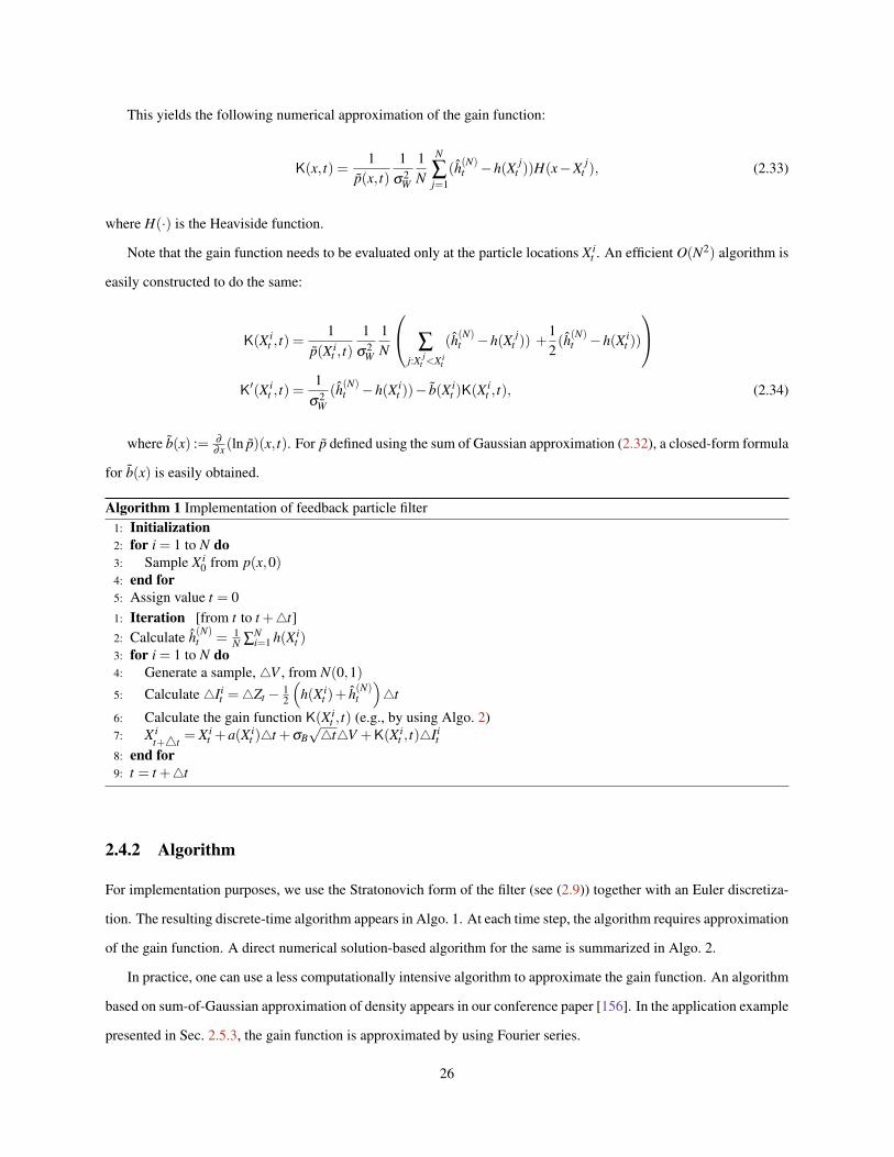
This yields the following numerical approximation of the gain function:
K(x, t) =1
p(x, t)1
σ2W
1N
N
∑j=1
(h(N)t −h(X j
t ))H(x−X jt ), (2.33)
where H(·) is the Heaviside function.
Note that the gain function needs to be evaluated only at the particle locations X it . An efficient O(N2) algorithm is
easily constructed to do the same:
K(X it , t) =
1p(X i
t , t)1
σ2W
1N
∑j:X j
t <X it
(h(N)t −h(X j
t )) +12(h(N)
t −h(X it ))
K′(X i
t , t) =1
σ2W(h(N)
t −h(X it ))− b(X i
t )K(X it , t), (2.34)
where b(x) := ∂
∂x (ln p)(x, t). For p defined using the sum of Gaussian approximation (2.32), a closed-form formula
for b(x) is easily obtained.
Algorithm 1 Implementation of feedback particle filter1: Initialization2: for i = 1 to N do3: Sample X i
0 from p(x,0)4: end for5: Assign value t = 01: Iteration [from t to t +4t]2: Calculate h(N)
t = 1N ∑
Ni=1 h(X i
t )3: for i = 1 to N do4: Generate a sample, 4V , from N(0,1)5: Calculate 4Ii
t =4Zt − 12
(h(X i
t )+ h(N)t
)4t
6: Calculate the gain function K(X it , t) (e.g., by using Algo. 2)
7: X it+4t = X i
t +a(X it )4t +σB
√4t4V +K(X i
t , t)4Iit
8: end for9: t = t +4t
2.4.2 Algorithm
For implementation purposes, we use the Stratonovich form of the filter (see (2.9)) together with an Euler discretiza-
tion. The resulting discrete-time algorithm appears in Algo. 1. At each time step, the algorithm requires approximation
of the gain function. A direct numerical solution-based algorithm for the same is summarized in Algo. 2.
In practice, one can use a less computationally intensive algorithm to approximate the gain function. An algorithm
based on sum-of-Gaussian approximation of density appears in our conference paper [156]. In the application example
presented in Sec. 2.5.3, the gain function is approximated by using Fourier series.
26
Algorithm 2 Synthesis of gain function K(x, t)
1: Calculate ht ≈ h(N)t ;
2: Approximate p(x, t) as a sum of Gaussian:
p(x, t)≈ p(x, t) =1N
N
∑j=1
q jt (x),
where q jt (x) =
1√2πε
exp(− (x−X j
t )2
2ε
).
3: Calculate the gain function
K(x, t) =1
p(x, t)1
σ2W
1N
N
∑j=1
(h(N)
t −h(X jt ))
H(x−X jt ),
where H(·) is the Heaviside function.
2.4.3 Further Remarks on the BVP
Recall that the solution of the nonlinear filtering problem is given by the Kushner-Stratonovich nonlinear evolution
PDE. The feedback particle filter instead requires, at each time t, a solution of the linear BVP (2.8) to obtain the gain
function K.
We make the following remarks:
1) There are close parallels between the proposed algorithm and the vortex element method (VEM) developed by
Chorin and others for solution of the Navier-Stokes evolution equation; cf., [42, 106]. In VEM, as in the feedback
particle filter, one obtains the solution of a Navier-Stokes equation by flowing a large number of particles. The
vector-field for the particles is obtained by solving a linear BVP at each time.
Algorithms based on VEM are popular in the large Reynolds number regime when the domain is not too compli-
cated. The latter requirement is necessary to obtain solution of the linear BVP in tractable fashion [75].
2) One may ask what is the benefit, in terms of accuracy and computational cost, of the feedback particle filter-based
solution when compared to a direct solution of the nonlinear evolution equation (Kushner-Stratonovich PDE), or
even its linear counterpart (Zakai equation)?
The key point, we believe, is robustness on account of the feedback control structure. Specifically, the self-
correcting property of the feedback provides robustness, allowing one to tolerate a degree of uncertainty inherent
in any model or approximation scheme. This is expected to yield accurate solutions in a computationally efficient
manner. A complete answer will require further analysis, and as such reflects an important future direction.
3) The biggest computational cost of our approach is the need to solve the BVP at each time-step, that additionally
requires one to approximate the density. We are encouraged however by the extensive set of tools in feedback
27

0 5 10
0
1
-1
2
0 5 10 0 5 10
N = 10
t0.1
0.15
0.2
0.25
0.1
0.15
0.2
0.254 N = 104 N = 102X(t)
µN (t)
State
Cond.mean M.C. est.
Cond. cov.
Cond. cov. M.C. est.
Σ(t)
ΣN (t)
Cond. cov.
Cond. cov. M.C. est.
Σ(t)
ΣN (t)
Figure 2.2: (a) Comparison of the true state Xt and the conditional mean µ(N)t . (b) and (c) Plots of estimated
conditional covariance with N = 10,000 and N = 100 particles, respectively. For comparison, the true conditionalcovariance obtained using Kalman filtering equations is also shown.
control: after all, one rarely needs to solve the HJB equations in closed-form to obtain a reasonable feedback
control law. Moreover, there are many approaches in nonlinear and adaptive control to both approximate control
laws as well as learn/adapt these in online fashion; cf., [14].
2.5 Numerics
2.5.1 Linear Gaussian Case
Consider the linear system:
dXt = α Xt dt + dBt , (2.35a)
dZt = γ Xt dt +σW dWt , X0 ∼ N(1,1) , (2.35b)
where Bt,Wt are mutually independent standard Wiener process, and parameters α =−0.5, γ = 3 and σW = 0.5.
Each of the N particles is described by the linear SDE,
dX it = α X i
t dt + dBit +
γ Σ(N)t
σ2W
[dZt − γX i
t + µ(N)t
2dt] , (2.36)
where Bit are mutually independent standard Wiener process; the particle system is initialized by drawing initial
conditions X i0N
i=1 from the distribution N(1,1), and the parameter values are chosen according to the model.
In the simulation discussed next, the mean µ(N)t and the variance Σ
(N)t are obtained from the ensemble X i
t Ni=1
according to (2.30).
Fig. 2.2 summarizes some of the results of the numerical experiments: Part (a) depicts a sample path of the state
Xt and the mean µ(N)t obtained using a particle filter with N = 10,000 particles. Part (b) provides a comparison
28

(b) TimeBPFFPF
(a) Error FPF −0.500.5BPF −0.50
Bootstrap (BPF)
Feedback (FPF)
Figure 2.3: Comparison of (a) the mse, (b) the computational time using feedback particle filter and the bootstrapparticle filter.
between the estimated variance Σ(N)t and the true error variance Σt that one would obtain by using the Kalman filtering
equations. The accuracy of the results is sensitive to the number of particles. For example, part (c) of the figure
provides a comparison of the variance with N = 100 particles.
Comparison with the bootstrap filter: We next provide a performance comparison between the feedback particle
filter and the bootstrap particle filter for the linear problem (2.35a, 2.35b) in regard to both error and running time.
For the linear filtering problem, the optimal solution is given by the Kalman filter. We use this solution to define
the relative mean-squared error:
mse =1T
∫ T
0
(Σ(N)t −Σt
Σt
)2
dt, (2.37)
where Σt is the error covariance using the Kalman filter, and Σ(N)t is its approximation using the particle filter.
Fig. 2.3(a) depicts a comparison between mse obtained using the feedback particle filter (2.36) and the bootstrap
filter. The latter implementation is based on an algorithm taken from Ch. 9 of [7]. For simulation purposes, we used a
range of values of α ∈ −0.5,0,0.5, γ = 3, σB = 1, σW = 0.5, 4t = 0.01, and T = 50. The plot is generated using
simulations with N = 20,50,100,200,500,1000 particles.
These numerical results suggest that feedback can help reduce the high variance that is sometimes observed with
the conventional particle filter. The variance issue can be especially severe if the signal process (2.1a) is unstable
(e.g., α > 0 in (2.35a)). In this case, individual particles can exhibit numerical instabilities due to time-discretization,
floating point representation etc. With α > 0, our numerical simulations with the bootstrap filter “blew-up” (similar
conclusions were also arrived independently in [51]) while the feedback particle filter is provably stable based on
observability of the model (2.35a)-(2.35b) (see Fig. 2.3 mse plot with α = 0.5).
Fig. 2.3(b) depicts a comparison between computational time for the two filtering algorithms on the same problem.
The time is given in terms of computation time per iteration cycle (see Algo. 1 in Sec. 2.4.2) averaged over 100 trials.
29
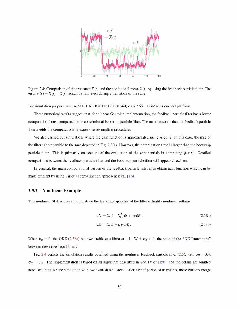
0 20 40 60 80 100 120
−1
0
1
X(t)
E(t)X(t)
Figure 2.4: Comparison of the true state X(t) and the conditional mean X(t) by using the feedback particle filter. Theerror E (t) = X(t)− X(t) remains small even during a transition of the state.
For simulation purpose, we use MATLAB R2011b (7.13.0.564) on a 2.66GHz iMac as our test platform.
These numerical results suggest that, for a linear Gaussian implementation, the feedback particle filter has a lower
computational cost compared to the conventional bootstrap particle filter. The main reason is that the feedback particle
filter avoids the computationally expensive resampling procedure.
We also carried out simulations where the gain function is approximated using Algo. 2. In this case, the mse of
the filter is comparable to the mse depicted in Fig. 2.3(a). However, the computation time is larger than the bootstrap
particle filter. This is primarily on account of the evaluation of the exponentials in computing p(x, t). Detailed
comparisons between the feedback particle filter and the bootstrap particle filter will appear elsewhere.
In general, the main computational burden of the feedback particle filter is to obtain gain function which can be
made efficient by using various approximation approaches; cf., [154].
2.5.2 Nonlinear Example
This nonlinear SDE is chosen to illustrate the tracking capability of the filter in highly nonlinear settings,
dXt = Xt(1−X2t )dt +σB dBt , (2.38a)
dZt = Xt dt +σW dWt . (2.38b)
When σB = 0, the ODE (2.38a) has two stable equilibria at ±1. With σB > 0, the state of the SDE “transitions”
between these two “equilibria”.
Fig. 2.4 depicts the simulation results obtained using the nonlinear feedback particle filter (2.5), with σB = 0.4,
σW = 0.2. The implementation is based on an algorithm described in Sec. IV of [156], and the details are omitted
here. We initialize the simulation with two Gaussian clusters. After a brief period of transients, these clusters merge
30

into a single cluster, which adequately tracks the true state including the transition events.
2.5.3 Application: Nonlinear Oscillators
We consider the filtering problem for a nonlinear oscillator:
dθt = ω dt +σB dBt mod 2π, (2.39)
dZt = h(θt)dt +σW dWt , (2.40)
where ω is the frequency, h(θ)= 12 [1+cos(θ)], and Bt and Wt are mutually independent standard Wiener process.
For numerical simulations, we pick ω = 1 and the standard deviation parameters σB = 0.5 and σW = 0.4. We consider
oscillator models because of their significance to applications including neuroscience; cf., [160].
The feedback particle filter is given by:
dθit = ω dt +σB dBi
t +K(θ it , t)
[dZt −
12(h(θ i
t )+ ht)dt]
mod 2π, (2.41)
i = 1, ...,N, where the function K(θ , t) is obtained via the solution of the E-L equation:
− ∂
∂θ
(1
p(θ , t)∂
∂θp(θ , t)K(θ , t)
)=− sinθ
2σ2W. (2.42)
Although the equation (2.42) can be solved numerically to obtain the optimal control function K(θ , t), here we
investigate a solution based on perturbation method. Suppose, at some time t, p(θ , t) = 12π
=: p0, the uniform density.
In this case, the E-L equation is given by:
∂θθ K =sinθ
2σ2W.
A straightforward calculation shows that the solution in this case is given by
K(θ , t) =− sinθ
2σ2W
=: K0(θ). (2.43)
To obtain the solution of the E-L equation (2.42), we assume that the density p(θ , t) is a small harmonic perturba-
tion of the uniform density. In particular, we express p(θ , t) as:
p(θ , t) = p0 + ε p(θ , t), (2.44)
where ε is a small perturbation parameter. Since p(θ , t) is a density,∫ 2π
0 p(θ , t)dθ = 0.
31

We are interested in obtaining a solution of the form:
K(θ , t) = K0(θ)+ εK(θ , t). (2.45)
On substituting the ansatz (2.44) and (2.45) in (2.42), and retaining only O(ε) term, we obtain the following linearized
equation:
∂θθ K =−2π∂θ [(∂θ p)K0]. (2.46)
The linearized E-L equation (2.46) can be solved easily by considering a Fourier series expansion of ε p(θ , t):
ε p(θ , t) = Pc(t)cosθ +Ps(t)sinθ +h.o.h, (2.47)
where “h.o.h” denotes the terms due to higher order harmonics. The Fourier coefficients are given by,
Pc(t) =1π
∫ 2π
0p(θ , t)cosθ dθ , Ps(t) =
1π
∫ 2π
0p(θ , t)sinθ dθ .
For a harmonic perturbation, the solution of the linearized E-L equation (2.46) is given by:
εK(θ , t) =π
4σ2W(Pc(t)sin2θ −Ps(t)cos2θ)
=: K1(θ ;Pc(t),Ps(t)) (2.48)
For “h.o.h” terms in the Fourier series expansion (2.47) of the density in p(θ , t), the linearized E-L equation (2.46)
can be solved in a similar manner. In numerical simulation provided here, we ignore the higher order harmonics, and
use a control input as summarized in the following proposition:
Proposition 2.5.1 Consider the E-L equation (2.42) where the density p(θ , t) is assumed to be a small harmonic
perturbation of the uniform density 12π
, as defined by (2.44) and (2.47). As ε → 0, the gain function is given by the
following asymptotic formula:
K(θ , t) = K0(θ)+K1(θ ;Pc(t),Ps(t))+o(ε), (2.49)
where Pc(t),Ps(t) denote the harmonic coefficients of density p(θ , t). For large N, these are approximated by using
the formulae:
Pc(t)≈1
πN
N
∑j=1
cosθ j(t), Ps(t)≈1
πN
N
∑j=1
sinθ j(t). (2.50)
We next discuss the result of numerical experiments. The particle filter model is given by (2.41) with gain function
32
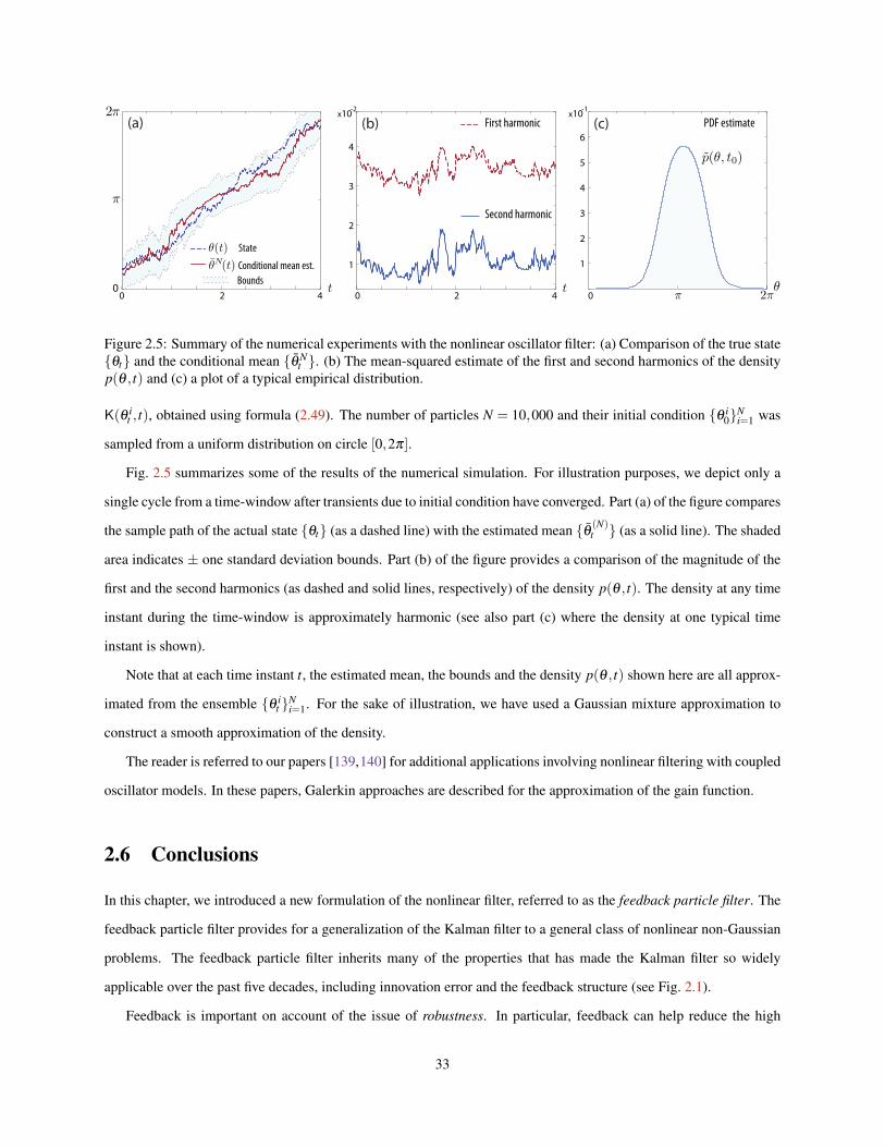
420420 0
1
2
3
4
1
2
3
4
5
6
t t θπ 2π
0
π
2π(a) (b) (c)
Bounds
State
Conditional mean est.
θ(t)
θN(t)
Second harmonic
First harmonic PDF estimatex10-2 x10⁻¹
p(θ, t0)
Figure 2.5: Summary of the numerical experiments with the nonlinear oscillator filter: (a) Comparison of the true stateθt and the conditional mean θ N
t . (b) The mean-squared estimate of the first and second harmonics of the densityp(θ , t) and (c) a plot of a typical empirical distribution.
K(θ it , t), obtained using formula (2.49). The number of particles N = 10,000 and their initial condition θ i
0Ni=1 was
sampled from a uniform distribution on circle [0,2π].
Fig. 2.5 summarizes some of the results of the numerical simulation. For illustration purposes, we depict only a
single cycle from a time-window after transients due to initial condition have converged. Part (a) of the figure compares
the sample path of the actual state θt (as a dashed line) with the estimated mean θ (N)t (as a solid line). The shaded
area indicates ± one standard deviation bounds. Part (b) of the figure provides a comparison of the magnitude of the
first and the second harmonics (as dashed and solid lines, respectively) of the density p(θ , t). The density at any time
instant during the time-window is approximately harmonic (see also part (c) where the density at one typical time
instant is shown).
Note that at each time instant t, the estimated mean, the bounds and the density p(θ , t) shown here are all approx-
imated from the ensemble θ it N
i=1. For the sake of illustration, we have used a Gaussian mixture approximation to
construct a smooth approximation of the density.
The reader is referred to our papers [139,140] for additional applications involving nonlinear filtering with coupled
oscillator models. In these papers, Galerkin approaches are described for the approximation of the gain function.
2.6 Conclusions
In this chapter, we introduced a new formulation of the nonlinear filter, referred to as the feedback particle filter. The
feedback particle filter provides for a generalization of the Kalman filter to a general class of nonlinear non-Gaussian
problems. The feedback particle filter inherits many of the properties that has made the Kalman filter so widely
applicable over the past five decades, including innovation error and the feedback structure (see Fig. 2.1).
Feedback is important on account of the issue of robustness. In particular, feedback can help reduce the high
33

variance that is sometimes observed in the conventional particle filter. Numerical results are presented to support this
claim (see Fig. 2.3).
Even more significantly, the structural aspects of the Kalman filter have been as important as the algorithm itself in
design, integration, testing and operation of a larger system involving filtering problems (e.g., navigation systems). We
show in later chapters that the feedback particle filter similarly provides an integrated framework, now for nonlinear
non-Gaussian problems. Details on the feedback particle filter-based algorithms for nonlinear filtering with additional
uncertainty are described in Chap. 6, Chap. 7.
34
Chapter 3
Existence, Uniqueness and Admissibility∗
3.1 Introduction
In this chapter, we generalize the scalar feedback particle filter in Chap. 2 to the general multivariable case. Specifi-
cally, we consider the multivariable filtering problem:
dXt = a(Xt)dt +σ(Xt)dBt , (3.1a)
dZt = h(Xt)dt + dWt , (3.1b)
where Xt ∈ Rd is the state at time t, Zt ∈ Rm is the observation vector, and Bt, Wt are two mutually independent
Wiener processes taking values in Rd and Rm. The mappings a(·) : Rd → Rd , h(·) : Rd → Rm and σ(·) : Rd → Rd×d
are C1 functions. The covariance matrix of the observation noise Wt is assumed to be positive definite. The function
h is a column vector whose j-th coordinate is denoted as h j (i.e., h = (h1,h2, . . . ,hm)T ). For notational ease, the
process noise Bt is assumed to be a standard Wiener process. By scaling, we may assume without loss of generality
that the covariance matrices associated with Bt, Wt are identity matrices.
The objective of the filtering problem is to estimate the posterior distribution of Xt given the history Zt := σ(Zs :
0≤ s≤ t). The posterior is denoted by p∗ as defined in (1.2).
The multivariable feedback particle filter is a controlled system. The dynamics of the ith particle have the following
gain feedback form,
dX it = a(X i
t )dt +σ(X it )dBi
t +K(X it , t)dIi
t +Ω(X it , t)dt, (3.2)
where Bit are mutually independent standard Wiener processes, Ii is similar to the innovation process that appears
in the nonlinear filter,
dIit := dZt −
12(h(X i
t )+ h)dt, (3.3)
where h := E[h(X it )|Zt ]. In a numerical implementation, we approximate h≈ 1
N ∑Ni=1 h(X i
t ) =: h(N).
∗This chapter is an extension of the published paper [154].
35

The gain function K is obtained as a solution to an Euler-Lagrange boundary value problem (E-L BVP): For
j = 1,2, . . . ,m, the function φ j is a solution to the second-order differential equation,
∇ · (p(x, t)∇φ j(x, t)) =−(h j(x)− h j)p(x, t),∫φ j(x, t)p(x, t)dx = 0,
(3.4)
where p denotes the conditional distribution of X it given Zt . In terms of these solutions, the gain function is given by
[K]l j =∂φ j
∂xl. (3.5)
Note that the gain function needs to be obtained for each value of time t.
Finally, Ω = (Ω1,Ω2, ...,Ωd)T is the Wong-Zakai correction term:
Ωl(x, t) :=12
d
∑k=1
m
∑s=1
Kks(x, t)∂ Kls
∂xk(x, t). (3.6)
The controlled system (3.2)-(3.6) is called the multivariable feedback particle filter.
The main results of this chapter are as follows:
• Consistency. The feedback particle filter (3.2) is consistent with the nonlinear filter, given consistent initializations
p( · ,0) = p∗( · ,0).
Consequently, if the initial conditions X i0N
i=1 are drawn from the initial distribution p∗( · ,0) of X0, then, as
N→ ∞, the empirical distribution of the particle system approximates the posterior distribution p∗( · , t) for each t.
•Well-posedness. A weak formulation of (3.4) is introduced, and used to prove an existence-uniqueness result for φ j
in a suitable function space. Certain apriori bounds are derived for the gain function to show that the resulting control
input in (3.2) is admissible (That is, the filter (3.2) is well-posed in the Ito sense).
• Numerical algorithms. Based on the weak formulation, a Galerkin finite-element algorithm is proposed for ap-
proximation of the gain function K(x, t). The algorithm is completely adapted to data (That is, it does not require an
explicit approximation of p(x, t) or computation of derivatives). Certain closed-form expressions for gain function are
derived in certain special cases. The conclusions are illustrated with numerical examples.
• Characterization of the feedback gain. The Smoluchowski equation models a d-dimensional gradient flow with
“noise”:
dΦt =−∇G (Φt)dt +√
2dξt , (3.7)
where ξ is a standard Wiener process. It is regarded as the original MCMC algorithm: Under general conditions it is
36

ergodic, with (unnormalized) stationary distribution e−G . The BVP (3.4) can be expressed as an instance of Poisson’s
equation for this diffusion,
Dφ j =−(h j− h j) , 1≤ j ≤ m , (3.8)
where D is the differential generator for the Smoluchowski equation, with potential G = − log p. Subject to growth
conditions on h and p, this implies the mean-integral representation for the vector-valued function,
φ j(x) =∫
∞
0E[h j(Φt)− h j |Φ0 = x] dt. (3.9)
This representation also suggests an alternate proof of well-posedness and construction of numerical algorithms;
cf., [71]. This will be the subject of future work.
3.1.1 Comparison with Relevant Literature
The feedback particle filter is originally motivated by recent development in mean-field games, but the focus there has
been primarily on optimal control [79, 160].
In nonlinear filtering, there are two directly related works: Crisan and Xiong [45], and Mitter and Newton [117].
In each of these papers, a controlled system is introduced, of the form
dX it =
(a(X i
t )+u(X it , t))
dt +σB(X it )dBi
t .
The objective is to choose the control input to obtain a solution of the nonlinear filtering problem.
The approach in [117] is based on consideration of a finite-horizon optimal control problem. It leads to an HJB
equation whose solution yields the optimal control input.
The work of Crisan and Xiong is closer to ours in terms of both goals and approaches. Although we were not aware
of their work prior to submission of our original conference papers [156, 157], Crisan and Xiong provide an explicit
expression for a control law that is similar to the feedback particle filter, with some important differences. One, the
considerations of Crisan and Xiong (and also of Newton and Mitter) require introduction of a smooth approximation of
the process “ dZdt − ht ,” which we avoid with our formulation. Two, the filter derived in Crisan and Xiong has a structure
based on a gain feedback with respect to the smooth approximation, while the feedback particle filter is based on a
modified formula for the innovation error Iit as given in (3.3). This formula is fundamental to construction of particle
filters in continuous time settings. We clarify here that the formula for innovation error is not assumed, rather it comes
about as a result of the analysis of the variational problem.
Remarkably, both the feedback particle filter and Crisan and Xiong’s filter require solution of the same boundary
37

value problem, and as such have the same computational complexity. The BVP is solved to obtain the gain function.
However, the particular solution described in Crisan and Xiong for the BVP may not work in all cases, including the
linear Gaussian case. Additional discussion appears in Sec. 3.2.4.
Apart from these works, Daum and Huang have introduced the information flow filter for the continuous-discrete
time filtering problem [51]. Although an explicit formula for the filter is difficult to obtain, a closely related form of
the boundary value problem appears in their work. There is also an important discussion of both the limitations of the
conventional particle filter, and the need to incorporate feedback to ameliorate these issues. Several numerical exper-
iments are presented that describe high variance and robustness issues, especially where signal models are unstable.
These results provide significant motivation to the work described here.
3.1.2 Outline
The outline of the remainder of this chapter is as follows. The nonlinear filter is introduced in Sec. 3.2. Consistency
result is shown in Sec. 3.2.3, followed by a comparison with Crisan and Xiong’s filter in Sec. 3.2.4. The weak
formulation of the BVP appears in Sec. 3.3 where well-posedness results are also derived. Algorithms are discussed
in Sec. 3.4 and numerical examples in Sec. 3.5.
3.2 Multivariable Feedback Particle Filter
Consider the continuous time filtering problem (3.1a, 3.1b) introduced in Sec. 3.1.
We denote as p∗(x, t) the conditional distribution of Xt given Zt = σ(Zs : s ≤ t). The evolution of p∗(x, t) is
described by the Kushner-Stratonovich (K-S) equation:
dp∗ = L † p∗ dt +(h− h)T (dZt − hdt)p∗, (3.10)
where h =∫
h(x)p∗(x, t)dx and L † p∗ =−∇ · (p∗a)+ 12 ∑
dl,k=1
∂ 2
∂xl∂xk
(p∗[σσT ]lk
).
3.2.1 Belief State Dynamics & Control Architecture
The model for the particle filter is given by,
dX it = a(X i
t )dt +σ(X it )dBi
t +u(X it , t)dt +K(X i
t , t)dZt︸ ︷︷ ︸dU i
t
, (3.11)
38
where X it ∈ Rd is the state for the ith particle at time t, and Bi
t are mutually independent standard Wiener processes.
We assume the initial conditions X i0N
i=1 are i.i.d., independent of Bit, and drawn from the initial distribution p∗(x,0)
of X0. Both Bit and X i
0 are also assumed to be independent of Xt ,Zt . Note that the gain function K(x, t) is a d×m
matrix and u(x, t) ∈ Rd .
We impose admissibility requirements on the control input U it in (3.11):
Definition 3 (Admissible Input) The control input U it is admissible if the random variables u(x, t) and K(x, t) are
Zt =σ(Zs : s≤ t) measurable for each t. And for each t, E[|u|] :=E[∑l |ul(X it , t)|]<∞ and E[|K|2] :=E[∑l j |Kl j(X i
t , t)|2]<
∞.
Recall that there are two types of conditional distributions of interest in our analysis:
1. p(x, t): Defines the conditional dist. of X it given Zt .
2. p∗(x, t): Defines the conditional dist. of Xt given Zt .
The functions u(x, t),K(x, t) are said to be optimal if p≡ p∗. That is, given p∗(·,0) = p(·,0), our goal is to choose
u,K in the feedback particle filter so that the evolution equations of these conditional distributions coincide (see
(3.10) and (3.12)).
The evolution equation for the belief state is described in the next result. The proof is identical to the proof in the
scalar case (see Proposition 2 in [156]). It is omitted here.
Proposition 3.2.1 Consider the process X it that evolves according to the particle filter model (3.11). The conditional
distribution of X it given the filtration Zt , p(x, t), satisfies the forward equation
dp = L † pdt−∇ · (pK)dZt −∇ · (pu)dt +12
d
∑l,k=1
∂ 2
∂xl∂xk
(p[KKT ]lk
)dt. (3.12)
3.2.2 General Form of the Feedback Particle Filter
The general form of the feedback particle filter is obtained by choosing u,K as the solution to a certain E-L BVP
based on p. The function K is a solution to
∇ · (pK) =−(h− h)T p, (3.13)
and the function u is obtained as
u(x, t) =−12
K(x, t)(h(x)+ h
)+Ω(x, t). (3.14)
The reader is referred to our earlier paper [156] for additional justification regarding these choices.
39
If one further assumes that the control input U it is admissible, a short calculation shows that the feedback particle
filter is consistent with the choice of u,K given by (3.13)-(3.14). This calculation appears in App. B.1.
3.2.3 Consistency with the Nonlinear Filter
To establish admissibility of the input U it requires additional assumptions on the density p and function h:
(i) Assumption A1 The probability density p(x, t) is of the form p(x, t) = e−G (x,t), where G (x, t) is a twice continuously
differentiable function with
|∇G |2−2∆G → ∞ as |x| → ∞. (3.15)
(ii) Assumption A2 The function h satisfies, ∫|h(x)|2 p(x, t)dx< ∞,
where |h(x)|2 := ∑ j |h j(x)|2. For admissibility of u, our arguments require additional assumptions:
(iii) Assumption A3 The second derivatives of G (x, t) with respect to x are uniformly bounded at each t, i.e., | ∂ 2G∂x j∂xk
(x, t)| ≤
c2(t) for all x ∈ Rd , t > 0.
(iv) Assumption A4 The first (weak) derivatives of h satisfy
∫|∇h(x)|2 p(x, t)dx< ∞,
where |∇h(x)|2 := ∑ jk |∂h j∂xk
(x)|2.
Under these assumptions, it is shown in Theorem 3.3.1 that the gradient-form representation (3.4) of the E-L
BVP (3.13) is uniquely obtained to give φ and thence K.
The admissibility of the resulting control input is established in Corollary 3.3.1. Theorem 3.3.1 and Corollary 3.3.1
are stated and proved in Sec. 3.3.
The following theorem then shows that the two evolution equations (3.10) and (3.12) are identical. The proof
appears in App. B.1.
Theorem 3.2.2 Consider the two evolution equations for p and p∗, defined according to the solution of the forward
equation (3.12) and the K-S equation (3.10), respectively. Suppose that the gain function K(x, t) is obtained according
to (3.4)-(3.5). Then, provided p( · ,0) = p∗( · ,0), we have for all t ≥ 0,
p( · , t) = p∗( · , t).
40

3.2.4 Comparison with Crisan and Xiong’s Filter
For ease of presentation, consider the model (3.1a)-(3.1b) where the observation process Zt ∈ R is real-valued. To aid
comparison with Crisan and Xiong’s work, we express the feedback particle filter in its Stratonovich form:
dX it = a(X i
t )dt +σ(X it )dBi
t +K(X it , t) dIi
t , (3.16)
where the gain function K(x, t) = (K1,K2, ...,Kd)T is vector-valued. It is given by the solution of a BVP:
∇ · (pK) =−(h− ht)p. (3.17)
Following the work of Crisan and Xiong [45], we might assume the following representation in an attempt to
solve (3.17),
pK = ∇φ . (3.18)
where φ is assumed to be sufficiently smooth. Substituting (3.18) in (3.17) yields the Poisson equation,
∆φ =−(h− ht)p . (3.19)
A solution to Poisson’s equation with d ≥ 2 can be expressed in terms of Green’s function:
G(r) =
1
2πln(r) for d = 2;
1d(2−d)ωd
r2−d for d > 2 ,
where ωd is the volume of the unit ball in Rd . A solution to (3.19) is then given by,
φ(x) =− 1σ2
W
∫Rd
G(|y− x|)(h(y)− ht)p(y, t)dy,
where |y− x| :=(
∑dj=1(y j− x j)
2) 1
2is the Euclidean distance.
On taking the gradient and using (3.18), one obtains an explicit formula for the gain function:
K(x, t) =Γ(p,h)(x)
p(x, t)=: Kg(x, t), (3.20)
where Γ(p,g)(x) := 1dωd
∫ y−x|y−x|d (g(y)− g)p(y)dy.
While this leads to a solution to (3.17), it may not lead to an admissible control law. This difficulty arises in the
41

prior work of Crisan and Xiong. In [45] and in Sec. 4 of [150], a particle filter of the following form is presented by
the authors:
dX it = a(X i
t )dt +σ(X it )dBi
t +Kg(X it , t)( d
dtIt)
dt, (3.21)
where It is a certain smooth approximation obtained from the standard form of the innovation error It := Zt −∫ t
0 ht dt.
A consistency result is described for this filter.
We make the following comparisons:
1) Without taking a smooth approximation, the filter (3.21) is formally equivalent to the following SDE expressed here
in its Stratonovich form:
dX it = a(X i
t )dt +σ(X it )dBi
t +Kg(X it , t)
(dZt − ht dt
). (3.22)
In this case, using (3.12), it is straightforward to show that the consistency result does not hold. In particular, there
is an extra second order term that is not present in the K-S equation for evolution of the true posterior p∗(x, t).
2) The proposed feedback particle filter does not require a smooth approximation and yet achieves consistency. The
key breakthrough is the modified definition of the innovation error (compare (3.22) with (3.16)). Note that the
innovation error (3.3) is not assumed apriori but comes about via analysis of the variational problem. This is
one utility of introducing the variational formulation. Once the feedback particle filter has been derived, it is
straightforward to prove consistency (see the Proof of Thm. 3.2.2).
3) The computational overhead for the feedback particle filter and the filter of Crisan and Xiong are equal. Both
require the approximation of the integral (3.20), and division by (a suitable regularized approximation of) p(x, t).
Numerically, the Poisson equation formulation (3.19) of the E-L BVP (3.17) is convenient. There exist efficient
numerical algorithms to approximate the integral solution (3.20) for a system of N particles in arbitrary dimension;
cf., [75].
However, while appealing, the function Kg is not the correct form of the gain function in the multivariable case,
even for the linear Gaussian model: It is straightforward to verify that the Kalman gain is a solution of the boundary
value problem (3.17). Using the Kalman gain for the gain function in (3.16) yields the feedback particle filter for the
multivariable linear Gaussian case. The filter is described in Sec. 3.3.4.
However, the Kalman gain solution is not of the form (3.18). Thus, the integral solution (3.20) does not equal the
Kalman gain in the linear Gaussian case (for d ≥ 2).
Moreover, the gradient form solution is unbounded: |Kg(x, t)| → ∞ as |x| → ∞, and E[|Kg|] = E[|Kg|2] = ∞. A
proof is given in App. B.2.
It follows that the control input obtained using Kg is not admissible, and hence the Kolmogorov forward operator
42
is no longer valid. Filter implementations using Kg suffer from numerical issues on account of large unbounded gains.
In contrast, the feedback particle filter using the Kalman gain works both in theory and in practice.
The choice of gain function in the multivariable case requires careful consideration of the uniqueness of the solu-
tions of the BVP: The solution of (3.17) is not unique, even though uniqueness holds when pK is assumed to be of a
gradient-form. More details on the well-posedness result appear in Sec. 3.3.
Before closing this section, we note that [45, Proposition 2.4] concerns another filter that does not rely on smooth
approximation,
dX it = a(X i
t )dt +σ(X it )dBi
t +Kg(X it , t) dZt −
1σ2
W
Γ(p, 12 |h|2)(X i
t )
p(X it , t)
dt.
Our calculations indicate that consistency is also an issue for this filter. The issue with Kg also applies to this filter. A
more complete comparison needs further investigation.
3.3 Existence, Uniqueness and Admissibility
The aim of this section is to introduce a particular gradient-form solution of the BVP (3.13). The gradient-form so-
lution is obtained in terms of m real-valued functions φ1( · , t),φ2( · , t), . . . ,φm( · , t). For j = 1,2, . . . ,m, the function
φ j is a solution to,
∇ · (p(x, t)∇φ j(x, t)) =−(h j(x)− h j)p(x, t),∫φ j(x, t)p(x, t)dx = 0.
(3.23)
The normalization∫
φ j(x, t)p(x, t)dx = 0 is for convenience: If φ oj is a solution to the differential equation (3.23), we
obtain the desired normalization on subtracting its mean.
In terms of these solutions, the gain function is given by,
Kl j(x, t) =∂φ j
∂xl(x, t) , x ∈ Rd . (3.24)
It is straightforward to verify that K thus defined is a particular solution of the BVP (3.13).
3.3.1 Poisson’s Equation Interpretation
The differential equation (3.23) is solved for each t to give the m functions φ j( · , t) : 1 ≤ j ≤ m. On dividing each
side of this equation by p, elementary calculus leads to the equivalent equation (3.8), with generator D defined for C2
functions f via,
D f =−∇G ·∇ f +∆ f
43
and with G ( ·) = − log p( · , t). This is the differential generator for the Smoluchowski equation (3.7). It is shown
in [81] that this diffusion is exponentially ergodic under mild conditions on G . Consequently, E[h j(Φt)− h j |Φ0 = x]
converges to zero exponentially fast, subject to growth conditions on h j, and from this we can conclude that (3.9) is
well defined, and provides a solution to Poisson’s equation (3.8) [71].
Poisson’s equation can be regarded as the value function that arises in average-cost optimal control, and this is the
object of interest in the approximation techniques used in TD-learning for average-cost optimal control [114]. The
integral representation (3.9) suggests approximation techniques based on approximate models for the diffusion Φ.
The remainder of this section is devoted to showing existence and uniqueness of the solution of (3.23), and admis-
sibility of the resulting control input, obtained using gain function defined by (3.24).
3.3.2 Weak Formulation
Further analysis of this problem requires introduction of Hilbert spaces: L2(Rd ; p) is used to denote the Hilbert space
of functions on Rd that are square-integrable with respect to density p(·, t) (for a fixed time t); Hk(Rd ; p) is used to
denote the Hilbert space of functions whose first k-derivatives (defined in the weak sense) are in L2(Rd ; p). Denote
H10 (Rd ; p) :=
φ ∈ H1(Rd ; p)
∣∣∣ ∫ φ(x)p(x, t)dx = 0.
A function φ j ∈ H10 (Rd ; p) is said to be a weak solution of the BVP (3.23) if
∫∇φ j(x, t) ·∇ψ(x)p(x, t)dx =
∫(h j(x)− h j)ψ(x)p(x, t)dx, (3.25)
for all ψ ∈ H1(Rd ; p).
Denoting E[·] :=∫ ·p(x, t)dx, the weak form of the BVP (3.23) can also be expressed as
E[∇φ j ·∇ψ] = E[(h j− h j)ψ], ∀ ψ ∈ H1(Rd ; p). (3.26)
This representation is useful for the numerical algorithm described in Sec. 3.4.
3.3.3 Main Results
The existence-uniqueness result for the BVP (3.23) is described next — Its proof is given in App. B.3.
Theorem 3.3.1 Under Assumptions A1-A2, the BVP (3.23) possesses a unique weak solution φ j ∈ H10 (Rd ; p), satis-
44
fying ∫|∇φ j(x)|2 p(x, t)dx≤ 1
λ
∫|h j(x)− h j|2 p(x, t)dx. (3.27)
If in addition Assumptions A3-A4 hold, then φ j ∈ H2(Rd ; p) with
∫ ∣∣(D2φ j)(∇φ j)
∣∣ p(x, t)dx≤C(λ ; p)∫|∇h j|2 p(x, t)dx, (3.28)
where λ is (spectral gap) constant (see App. B.3) and C(λ ; p) = 1λ 3/2
(‖D2(log p)‖L∞
λ+1)1/2
.
The apriori bounds (3.27)-(3.28) are used to show that the control input for the feedback particle filter is admissible.
The proof is omitted.
Corollary 3.3.1 Suppose φ j is the weak solution of BVP (3.23) as described in Theorem 3.3.1. The gain function K is
obtained using (3.24) and u is given by (3.14). Then
E[|K|2]≤ 1λ
m
∑j=1
∫|h j(x)|2 p(x, t)dx,
E[|u|]≤(
1λ+C(λ ; p)
) m
∑j=1
∫ (|h j(x)|2 + |∇h j|2
)p(x, t)dx,
where C(λ ; p) is given in Theorem 3.3.1. That is, the resulting control input in (3.24) is admissible.
3.3.4 Linear Gaussian Case
Consider the linear system,
dXt = A Xt dt + dBt (3.29a)
dZt = H Xt dt + dWt (3.29b)
where A is an d× d matrix, and H is an m× d matrix. The initial distribution p∗(x,0) is Gaussian with mean vector
µ0 and covariance matrix Σ0.
The following proposition shows that the Kalman gain is a gradient-form solution of the multivariable BVP (3.13):
Proposition 3.3.2 Consider the d-dimensional linear system (3.29a)-(3.29b). Suppose p(x, t) is assumed to be Gaus-
sian: p(x, t) = 1
(2π)d2 |Σt |
12
exp(− 1
2 (x−µt)T Σ−1t (x−µt)
), where x = (x1,x2, ...,xd)
T , µt = (µ1t ,µ2t , . . . ,µdt)T is the
45

mean, Σt is the covariance matrix, and |Σt |> 0 denotes the determinant. A solution of the BVP (3.23) is given by,
φ j(x, t) =d
∑k=1
[ΣtHT ]k j(xk−µkt). (3.30)
Using (3.24), K(x, t) = ΣtHT (the Kalman gain) is the gradient form solution of (3.13).
The formula (3.30) is verified by direct substitution in the BVP (3.23) where the distribution p is multivariable
Gaussian.
The gain function yields the following form for the particle filter in this linear Gaussian model:
dX it = A X i
t dt + dBit +ΣtHT
(dZt −H
X it +µt
2dt). (3.31)
Now we show that p = p∗ in this case. That is, the conditional distributions of X and X i coincide, and are defined
by the well-known dynamic equations that characterize the mean and the variance of the continuous-time Kalman
filter.
Theorem 3.3.3 Consider the linear Gaussian filtering problem defined by the state-observation equations (3.29a)-
(3.29b). In this case the posterior distributions of Xt and X it are Gaussian, whose conditional mean and covariance
are given by the respective SDE and the ODE,
dµt = Aµt dt +ΣtHT(
dZt −Hµt dt)
ddt
Σt = AΣt +ΣtAT + I−ΣtHT HΣt
The result is verified by substituting p(x, t) = (2π)−d2 |Σt |−
12 exp
[− 1
2 (x−µt)T Σ−1t (x−µt)
]in the forward equa-
tion (3.12). The details are omitted, and because the result is a special case of Theorem 3.2.2.
In practice µt ,Σt are approximated as sample means and sample covariances from the ensemble X it N
i=1:
µt ≈ µ(N)t :=
1N
N
∑i=1
X it ,
Σt ≈ Σ(N)t :=
1N−1
N
∑i=1
(X it −µ
(N)t )2.
The resulting equation (3.31) for the ith particle is given by
dX it = A X i
t dt + dBit +Σ
(N)t HT
(dZt −H
X it +µ
(N)t
2dt
).
46
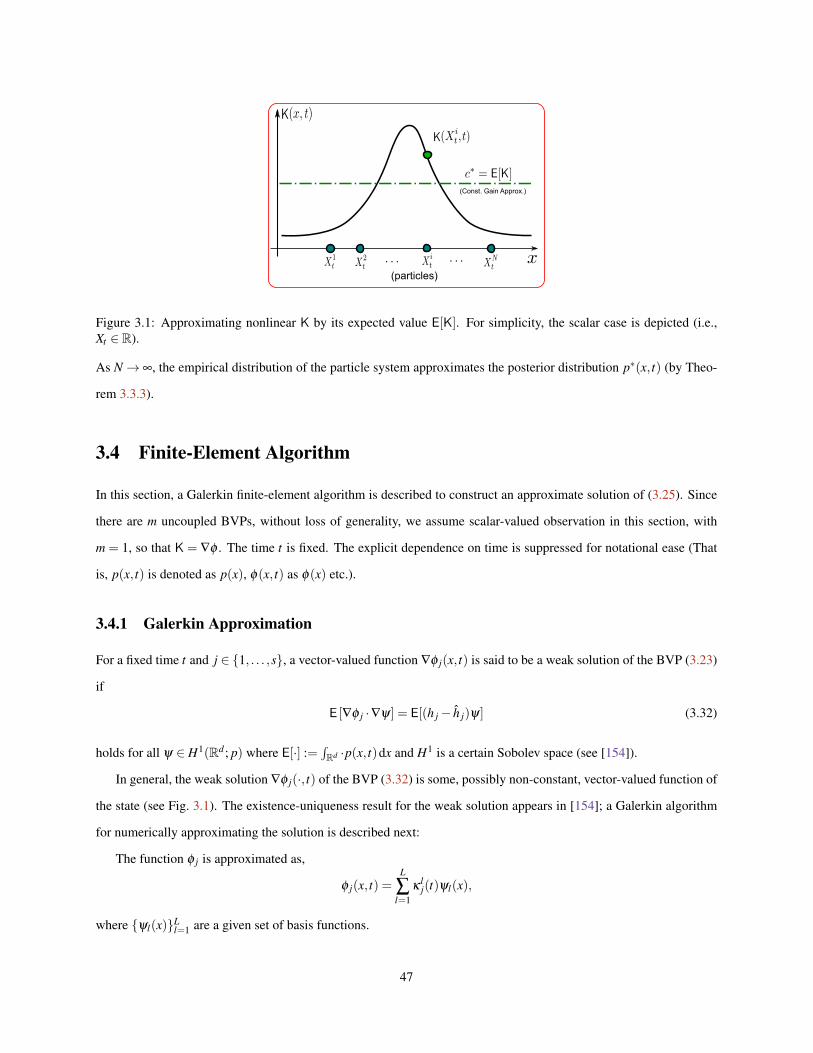
(Const. Gain Approx.)
(particles)
Figure 3.1: Approximating nonlinear K by its expected value E[K]. For simplicity, the scalar case is depicted (i.e.,Xt ∈ R).
As N→ ∞, the empirical distribution of the particle system approximates the posterior distribution p∗(x, t) (by Theo-
rem 3.3.3).
3.4 Finite-Element Algorithm
In this section, a Galerkin finite-element algorithm is described to construct an approximate solution of (3.25). Since
there are m uncoupled BVPs, without loss of generality, we assume scalar-valued observation in this section, with
m = 1, so that K = ∇φ . The time t is fixed. The explicit dependence on time is suppressed for notational ease (That
is, p(x, t) is denoted as p(x), φ(x, t) as φ(x) etc.).
3.4.1 Galerkin Approximation
For a fixed time t and j ∈ 1, . . . ,s, a vector-valued function ∇φ j(x, t) is said to be a weak solution of the BVP (3.23)
if
E [∇φ j ·∇ψ] = E[(h j− h j)ψ] (3.32)
holds for all ψ ∈ H1(Rd ; p) where E[·] :=∫Rd ·p(x, t)dx and H1 is a certain Sobolev space (see [154]).
In general, the weak solution ∇φ j(·, t) of the BVP (3.32) is some, possibly non-constant, vector-valued function of
the state (see Fig. 3.1). The existence-uniqueness result for the weak solution appears in [154]; a Galerkin algorithm
for numerically approximating the solution is described next:
The function φ j is approximated as,
φ j(x, t) =L
∑l=1
κlj(t)ψl(x),
where ψl(x)Ll=1 are a given set of basis functions.
47

The finite-dimensional approximation of (3.32) is to choose constants κ lj(t)L
l=1 – for each fixed time t – such
thatL
∑l=1
κlj(t) E[∇ψl ·∇ψ] = E[(h j− h j)ψ], ∀ ψ ∈ S, (3.33)
where S := spanψ1,ψ2, . . . ,ψL ⊂ H1(Rd ; p).
Denoting [A]kl = E[∇ψl ·∇ψk], bkj = E[(h j− h j)ψk], b j = (b1
j , . . . ,bLj ) and κ j = (κ1
j , . . . ,κLj ), the finite-dimensional
approximation (3.33) is expressed as a linear matrix equation:
Aκ j = b j.
In a numerical implementation, the matrix A and vector b j are approximated as,
[A]kl = E[∇ψl ·∇ψk]≈1N
N
∑i=1
∇ψl(X it ) ·∇ψk(X i
t ), (3.34)
bkj = E[(h j− h j)ψk]≈
1N
N
∑i=1
(h j(X it )− h j)ψk(X i
t ), (3.35)
where recall h j ≈ 1N ∑
Ni′=1 h j(X i′
t ). The important point to note is that the gain function is expressed in terms of averages
taken over the population.
3.4.2 Example 1: Constant Gain Approximation
Suppose χl = el , the canonical coordinate vector with value 1 for the lth coordinate and zero otherwise. The test
functions are the coordinate functions ψk(x) = xk for k = 1,2, . . . ,d. Denoting ψ(x) = (ψ1,ψ2, . . . ,ψd)T = x,
κ = E[K] = E[(h− h)ψ] =∫(h(x)− h)ψ(x)p(x)dx≈ 1
N
N
∑i=1
(h(X it )− h)X i
t . (3.36)
This formula yields the constant-gain approximation of the gain function.
The constant gain approximation is obtained by using the coordinate functions (x1,x2, . . . ,xd) as basis functions.
In this case,
κ j = E[(h j− h j)x]≈1N
N
∑i=1
X it
(h j(X i
t )−1N
N
∑i′=1
h j(X i′t )
)=: c(N)
j . (3.37)
Denoting C := [c(N)1 , . . . ,c(N)
s ], where c(N)j is a column vector for j∈1, . . . ,s, the gain function is succinctly expressed
as:
K =C. (3.38)
48

We refer to this solution as the constant gain approximation.
Remark 3 There is also a variational interpretation of these solutions. The constant gain approximation, for-
mula (3.38), is the best – in the least-square sense – constant approximation of the gain function (see Fig. 3.1).
Precisely, consider the following least-square optimization problem:
c∗j = arg minc j∈Rd
E[|∇φ j− c j|2].
By using a standard sum of square argument, we have
c∗j = E[∇φ j].
Even though φ j is unknown, a closed-form formula for constant vector c∗j can easily be obtained by using (3.32).
Specifically, by substituting ψ(x) = x = (x1,x2, . . . ,xd) in (3.32):
E[∇φ j] = E[(h j− h j)ψ] =∫Rd(h j(x)− h j) x p(x, t)dx.
This is also the first equality in (3.37).
Likewise, the Galerkin solution is the optimal least-square approximation in the function space S.
Remark 4 It is noted that if p is Gaussian and h is linear then, in the limit as N→∞, the constant gain approximation
equals the Kalman gain (see Sec. 3.3.4).
3.4.3 Example 2: Single-State Case
Consider a scalar example, where the density is a sum of Gaussian,
p(x)≈3
∑j=1
λjq j(x),
where q j(x) = q(x; µ j,Σ j) = 1√2πΣ j exp(− (x−µ j)2
2Σ j ), λ j > 0, ∑λ j = 1. The parameter values for λ j,µ j,Σ j are tabulated
in Table I.
In the scalar case, a direct numerical solution (DNS) of the gain function is obtained by numerically approximating
the integral
K(x) =− 1p(x)
∫ x
−∞
(h(y)− h)p(y)dy.
The DNS solution is used to provide comparisons with the approximate Galerkin solutions.
49
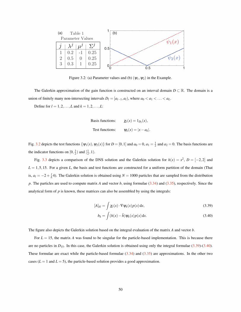
0 10.5
0.5
0
1
j µjλj Σj
1 -10.2 0.252 00.5 0.253 10.3 0.25
Table 1Parameter Values
(a) (b)
Figure 3.2: (a) Parameter values and (b) (ψ1,ψ2) in the Example.
The Galerkin approximation of the gain function is constructed on an interval domain D ⊂ R. The domain is a
union of finitely many non-intersecting intervals Dl = [al−1,al), where a0 < a1 < .. . < aL.
Define for l = 1,2, . . . ,L and k = 1,2, . . . ,L:
Basis functions: χl(x) = 1Dl (x),
Test functions: ψk(x) = |x−ak|.
Fig. 3.2 depicts the test functions ψ1(x),ψ2(x) for D = [0,1] and a0 = 0, a1 =12 and a2 = 0. The basis functions are
the indicator functions on [0, 12 ) and [ 1
2 ,1).
Fig. 3.3 depicts a comparison of the DNS solution and the Galerkin solution for h(x) = x2, D = [−2,2] and
L = 1,5,15. For a given L, the basis and test functions are constructed for a uniform partition of the domain (That
is, al =−2+ lL 4). The Galerkin solution is obtained using N = 1000 particles that are sampled from the distribution
p. The particles are used to compute matrix A and vector b, using formulae (3.34) and (3.35), respectively. Since the
analytical form of p is known, these matrices can also be assembled by using the integrals:
[A]kl =∫
χl(x) ·∇ψk(x)p(x)dx, (3.39)
bk =∫(h(x)− h)ψk(x)p(x)dx. (3.40)
The figure also depicts the Galerkin solution based on the integral evaluation of the matrix A and vector b.
For L = 15, the matrix A was found to be singular for the particle-based implementation. This is because there
are no particles in D15. In this case, the Galerkin solution is obtained using only the integral formulae (3.39)-(3.40).
These formulae are exact while the particle-based formulae (3.34) and (3.35) are approximations. In the other two
cases (L = 1 and L = 5), the particle-based solution provides a good approximation.
50
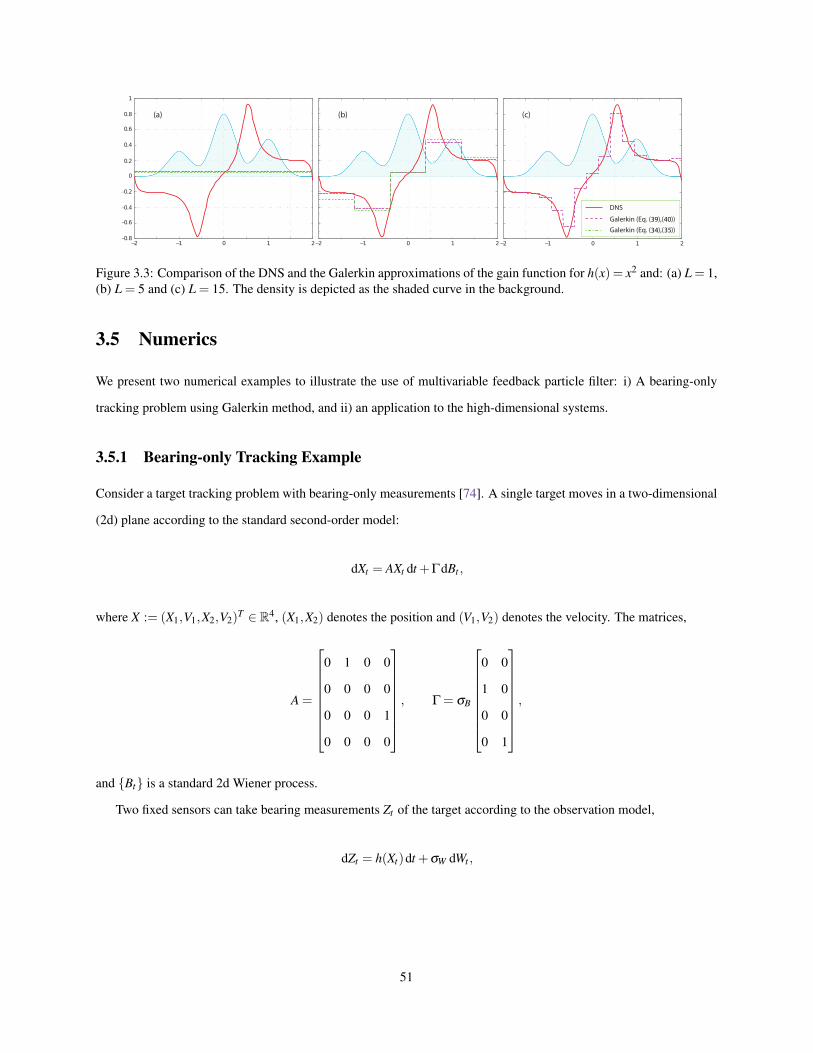
−2 −1 0 1 2
1
0.6
0.8
0.4
0
0.2
-0.2
-0.6
-0.4
-0.8−2 −1 0 1 2−2 −1 0 1 2
(a) (b) (c)
DNS
Galerkin (Eq. ( ),( ))
Galerkin (Eq. ( ),( ))
39 40
34 35
Figure 3.3: Comparison of the DNS and the Galerkin approximations of the gain function for h(x) = x2 and: (a) L = 1,(b) L = 5 and (c) L = 15. The density is depicted as the shaded curve in the background.
3.5 Numerics
We present two numerical examples to illustrate the use of multivariable feedback particle filter: i) A bearing-only
tracking problem using Galerkin method, and ii) an application to the high-dimensional systems.
3.5.1 Bearing-only Tracking Example
Consider a target tracking problem with bearing-only measurements [74]. A single target moves in a two-dimensional
(2d) plane according to the standard second-order model:
dXt = AXt dt +ΓdBt ,
where X := (X1,V1,X2,V2)T ∈ R4, (X1,X2) denotes the position and (V1,V2) denotes the velocity. The matrices,
A =
0 1 0 0
0 0 0 0
0 0 0 1
0 0 0 0
, Γ = σB
0 0
1 0
0 0
0 1
,
and Bt is a standard 2d Wiener process.
Two fixed sensors can take bearing measurements Zt of the target according to the observation model,
dZt = h(Xt)dt +σW dWt ,
51
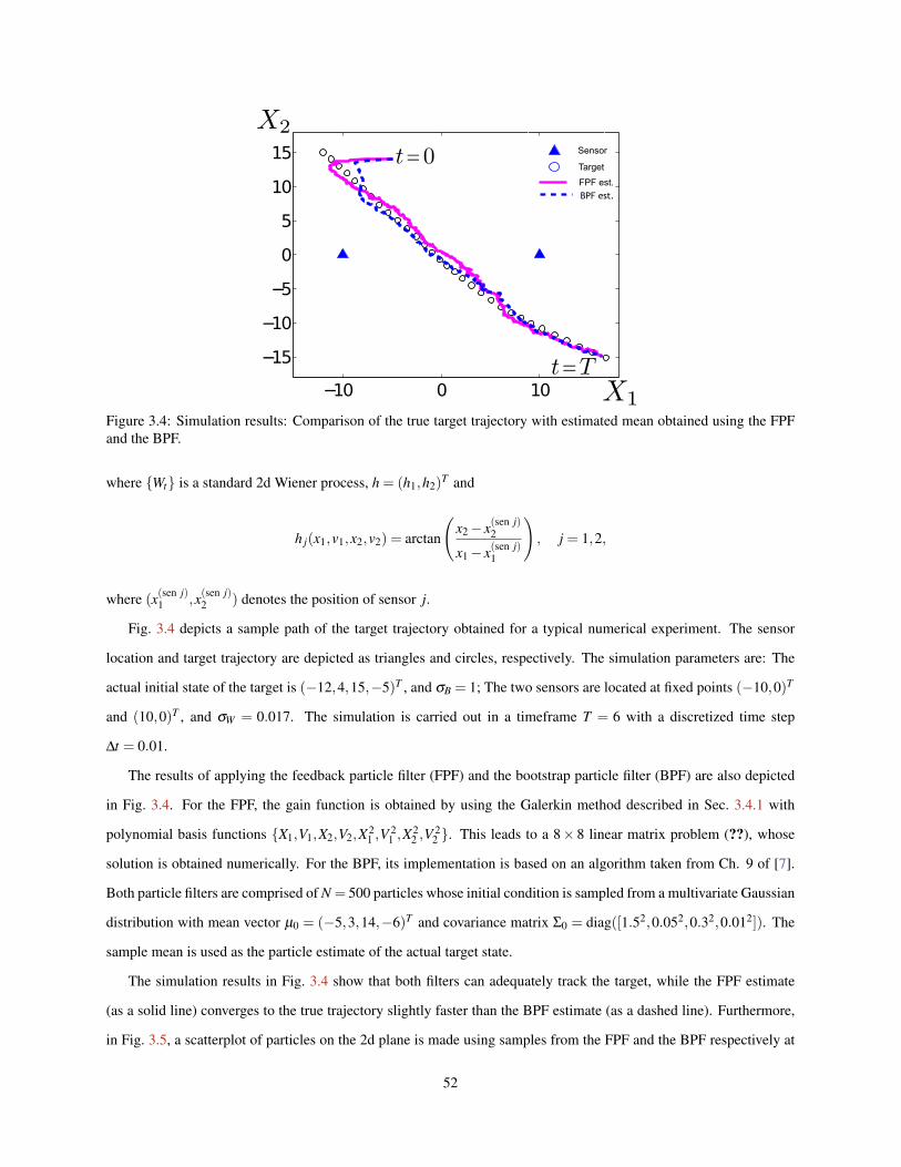
−10 0 10
−15
−10
−5
0
5
10
15 Sensor
Target
FPF est.
BPF est.
Figure 3.4: Simulation results: Comparison of the true target trajectory with estimated mean obtained using the FPFand the BPF.
where Wt is a standard 2d Wiener process, h = (h1,h2)T and
h j(x1,v1,x2,v2) = arctan
(x2− x(sen j)
2
x1− x(sen j)1
), j = 1,2,
where (x(sen j)1 ,x(sen j)
2 ) denotes the position of sensor j.
Fig. 3.4 depicts a sample path of the target trajectory obtained for a typical numerical experiment. The sensor
location and target trajectory are depicted as triangles and circles, respectively. The simulation parameters are: The
actual initial state of the target is (−12,4,15,−5)T , and σB = 1; The two sensors are located at fixed points (−10,0)T
and (10,0)T , and σW = 0.017. The simulation is carried out in a timeframe T = 6 with a discretized time step
∆t = 0.01.
The results of applying the feedback particle filter (FPF) and the bootstrap particle filter (BPF) are also depicted
in Fig. 3.4. For the FPF, the gain function is obtained by using the Galerkin method described in Sec. 3.4.1 with
polynomial basis functions X1,V1,X2,V2,X21 ,V
21 ,X
22 ,V
22 . This leads to a 8× 8 linear matrix problem (??), whose
solution is obtained numerically. For the BPF, its implementation is based on an algorithm taken from Ch. 9 of [7].
Both particle filters are comprised of N = 500 particles whose initial condition is sampled from a multivariate Gaussian
distribution with mean vector µ0 = (−5,3,14,−6)T and covariance matrix Σ0 = diag([1.52,0.052,0.32,0.012]). The
sample mean is used as the particle estimate of the actual target state.
The simulation results in Fig. 3.4 show that both filters can adequately track the target, while the FPF estimate
(as a solid line) converges to the true trajectory slightly faster than the BPF estimate (as a dashed line). Furthermore,
in Fig. 3.5, a scatterplot of particles on the 2d plane is made using samples from the FPF and the BPF respectively at
52
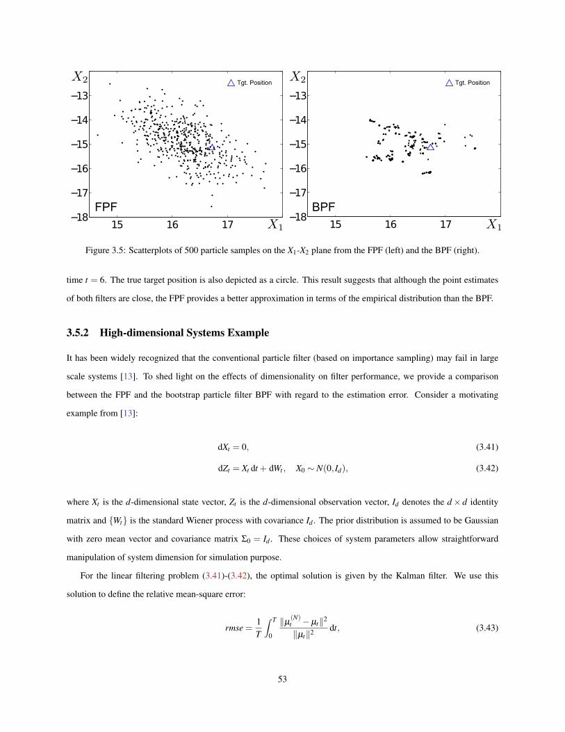
15 16 17−18
−17
−16
−15
−14
−13
15 16 17−18
−17
−16
−15
−14
−13Tgt. Position Tgt. Position
FPF BPF
Figure 3.5: Scatterplots of 500 particle samples on the X1-X2 plane from the FPF (left) and the BPF (right).
time t = 6. The true target position is also depicted as a circle. This result suggests that although the point estimates
of both filters are close, the FPF provides a better approximation in terms of the empirical distribution than the BPF.
3.5.2 High-dimensional Systems Example
It has been widely recognized that the conventional particle filter (based on importance sampling) may fail in large
scale systems [13]. To shed light on the effects of dimensionality on filter performance, we provide a comparison
between the FPF and the bootstrap particle filter BPF with regard to the estimation error. Consider a motivating
example from [13]:
dXt = 0, (3.41)
dZt = Xt dt + dWt , X0 ∼ N(0, Id), (3.42)
where Xt is the d-dimensional state vector, Zt is the d-dimensional observation vector, Id denotes the d× d identity
matrix and Wt is the standard Wiener process with covariance Id . The prior distribution is assumed to be Gaussian
with zero mean vector and covariance matrix Σ0 = Id . These choices of system parameters allow straightforward
manipulation of system dimension for simulation purpose.
For the linear filtering problem (3.41)-(3.42), the optimal solution is given by the Kalman filter. We use this
solution to define the relative mean-square error:
rmse =1T
∫ T
0
‖µ(N)t −µt‖2
‖µt‖2 dt, (3.43)
53
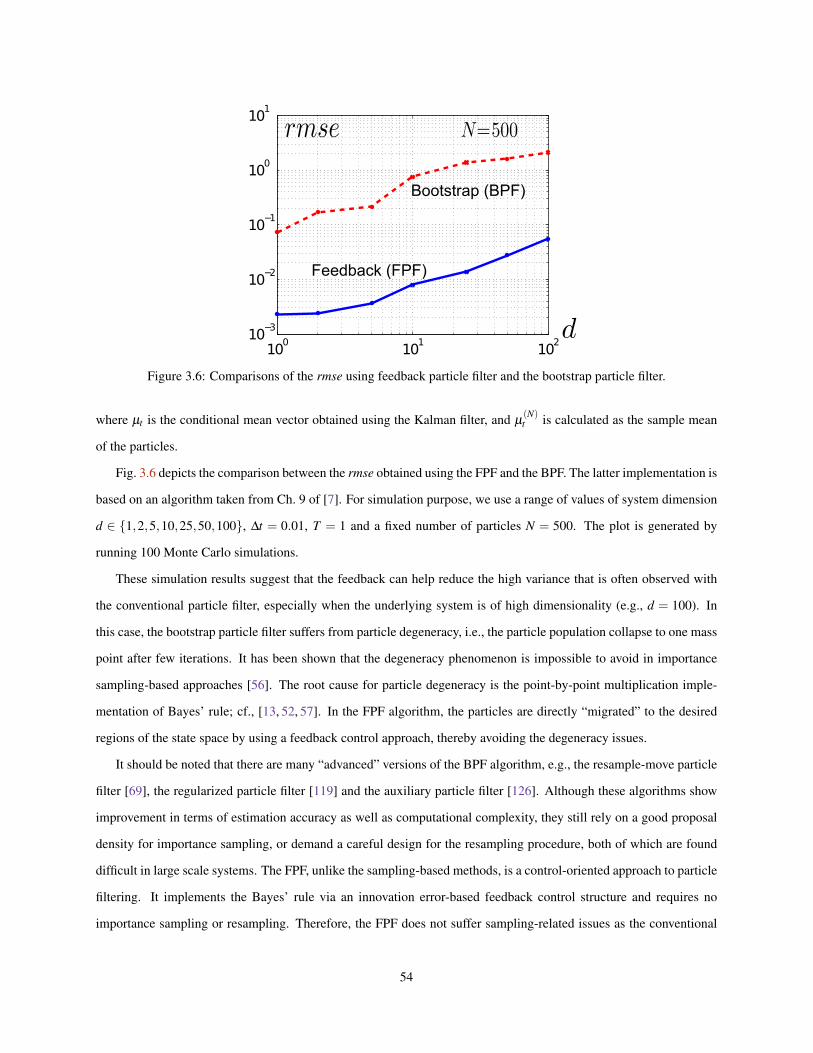
100
101
102
10−3
10−2
10−1
100
101
Bootstrap (BPF)
Feedback (FPF)
Figure 3.6: Comparisons of the rmse using feedback particle filter and the bootstrap particle filter.
where µt is the conditional mean vector obtained using the Kalman filter, and µ(N)t is calculated as the sample mean
of the particles.
Fig. 3.6 depicts the comparison between the rmse obtained using the FPF and the BPF. The latter implementation is
based on an algorithm taken from Ch. 9 of [7]. For simulation purpose, we use a range of values of system dimension
d ∈ 1,2,5,10,25,50,100, ∆t = 0.01, T = 1 and a fixed number of particles N = 500. The plot is generated by
running 100 Monte Carlo simulations.
These simulation results suggest that the feedback can help reduce the high variance that is often observed with
the conventional particle filter, especially when the underlying system is of high dimensionality (e.g., d = 100). In
this case, the bootstrap particle filter suffers from particle degeneracy, i.e., the particle population collapse to one mass
point after few iterations. It has been shown that the degeneracy phenomenon is impossible to avoid in importance
sampling-based approaches [56]. The root cause for particle degeneracy is the point-by-point multiplication imple-
mentation of Bayes’ rule; cf., [13, 52, 57]. In the FPF algorithm, the particles are directly “migrated” to the desired
regions of the state space by using a feedback control approach, thereby avoiding the degeneracy issues.
It should be noted that there are many “advanced” versions of the BPF algorithm, e.g., the resample-move particle
filter [69], the regularized particle filter [119] and the auxiliary particle filter [126]. Although these algorithms show
improvement in terms of estimation accuracy as well as computational complexity, they still rely on a good proposal
density for importance sampling, or demand a careful design for the resampling procedure, both of which are found
difficult in large scale systems. The FPF, unlike the sampling-based methods, is a control-oriented approach to particle
filtering. It implements the Bayes’ rule via an innovation error-based feedback control structure and requires no
importance sampling or resampling. Therefore, the FPF does not suffer sampling-related issues as the conventional
54
PF does. Rigorous convergence results of the FPF will be the subject of future work.
3.6 Conclusions
In this chapter, we introduce the feedback particle filter in the general multivariable setting. The main conclusions are:
(i) Consistency is established in the multivariate setting, as well as well-posedness of the associated PDE to obtain the
filter gain. The admissibility of the control input for the feedback particle filter is also proved.
(ii) The gain can be expressed as the gradient of a function, which is precisely the solution to Poissons equation for a
related MCMC diffusion (the Smoluchowski equation). This provides a bridge to MCMC as well as to approximate
optimal filtering approaches such as TD-learning, which can in turn be used to approximate the gain.
(iii) Motivated by a weak formulation of Poissons equation, a Galerkin finite-element algorithm is proposed for approx-
imation of the gain. Its performance is illustrated in numerical experiments.
The approximation of the gain function is at the core of the feedback particle filter algorithm. Future research
directions regarding the gain function approximation include but not limited to the following:
(i) How to choose the optimal basis function? The performance of FPF clearly depends the choice of basis functions
and the best way to do this is not clear.
(ii) Is it possible to write a differential equation for the gain function, i.e., use the gain function at time t to obtain the
gain function at time t +∆t? The Galerkin method, on the other hand, is memoryless (i.e., does not depend on the
history).
55
Chapter 4
Feedback Particle Filter forContinuous-Discrete Time Filtering∗
4.1 Introduction
The purpose of the present chapter is to introduce the feedback particle filter algorithm for the continuous-discrete
time nonlinear filtering problem. The motivation is two-fold: one is to derive the continuous-discrete time analogue
of the feedback control structure present in the continuous-time FPF algorithm. The other is to provide a comparison
to existing continuous discrete-time algorithms, specifically the work of Daum and Huang [51].
Filtering Problem: Consider the continuous-discrete time nonlinear filtering problem. The state process evolves in
continuous-time according to the stochastic differential equation (SDE) model:
dXt = a(Xt)dt + dBt , (4.1)
where Xt ∈ Rd is the state at time t, Bt is a d-dimensional standard Wiener process independent of X0, and a is
assumed to be a known C1 function so that SDE (4.1) has a pathwise unique solution for each initial X0.
The observations (measurements) are obtained at discrete-times t = tn according to the model:
Yn = h(Xtn)+Wn, (4.2)
where Yn ∈Rm, tn; n= 1,2, . . . is a strictly increasing sequence of observation sampling times, i.e., tn > tn−1, ∀n≥ 1;
the sequence tn is independent of Xt; Wn is a sequence of m-dimensional variables, each component of which is
independent and sampled from the Gaussian distribution; Wn is also independent of Xt and of tn. The function
h is a column vector whose j-th coordinate is denoted as h j (i.e., h = (h1,h2, . . . ,hm)). All components of h(x) are
assumed to be twice continuously differentiable in x.
The objective of the continuous-discrete time filtering problem (4.1)-(4.2) is to compute the conditional probability
density function (posterior) of Xt given the observation history (filtration) Zt := σYn : ∀n such that tn ∈ [0, t]. The
posterior distribution p∗ is defined the same as in (2.2).∗This chapter is an extension of the published paper [152].
56
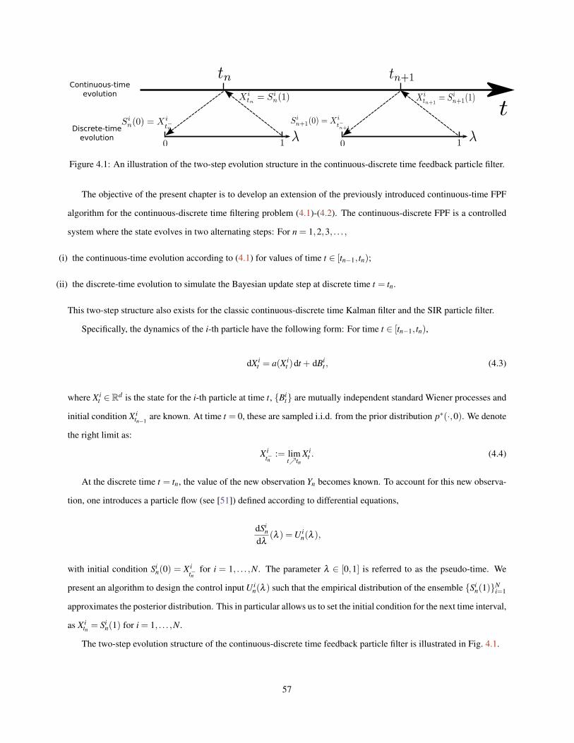
Continuous-timeevolution
Discrete-timeevolution
Figure 4.1: An illustration of the two-step evolution structure in the continuous-discrete time feedback particle filter.
The objective of the present chapter is to develop an extension of the previously introduced continuous-time FPF
algorithm for the continuous-discrete time filtering problem (4.1)-(4.2). The continuous-discrete FPF is a controlled
system where the state evolves in two alternating steps: For n = 1,2,3, . . . ,
(i) the continuous-time evolution according to (4.1) for values of time t ∈ [tn−1, tn);
(ii) the discrete-time evolution to simulate the Bayesian update step at discrete time t = tn.
This two-step structure also exists for the classic continuous-discrete time Kalman filter and the SIR particle filter.
Specifically, the dynamics of the i-th particle have the following form: For time t ∈ [tn−1, tn),
dX it = a(X i
t )dt + dBit , (4.3)
where X it ∈Rd is the state for the i-th particle at time t, Bi
t are mutually independent standard Wiener processes and
initial condition X itn−1
are known. At time t = 0, these are sampled i.i.d. from the prior distribution p∗(·,0). We denote
the right limit as:
X it−n
:= limttn
X it . (4.4)
At the discrete time t = tn, the value of the new observation Yn becomes known. To account for this new observa-
tion, one introduces a particle flow (see [51]) defined according to differential equations,
dSin
dλ(λ ) =U i
n(λ ),
with initial condition Sin(0) = X i
t−nfor i = 1, . . . ,N. The parameter λ ∈ [0,1] is referred to as the pseudo-time. We
present an algorithm to design the control input U in(λ ) such that the empirical distribution of the ensemble Si
n(1)Ni=1
approximates the posterior distribution. This in particular allows us to set the initial condition for the next time interval,
as X itn = Si
n(1) for i = 1, . . . ,N.
The two-step evolution structure of the continuous-discrete time feedback particle filter is illustrated in Fig. 4.1.
57
Recall that we denote conditional distribution of a particle X it given Zt by p:
∫x∈A
p(x, t)dx = PX it ∈ A|Zt,
and the empirical distribution formed by the “particle population” by p(N):
p(N)(A, t) =1N
N
∑i=1
1lX it ∈ A.
The control problem is to choose the control input U in(λ ) so that p approximate p∗, and consequently p(N) approxi-
mates p∗ for large N. The main result of this chapter is to derive an explicit formula for the optimal control input, and
demonstrate that under general conditions we obtain an exact match p = p∗ under optimal control.
The basic idea of particle flow is borrowed from Daum and Huang [48–51]. The control law – to obtain the
control input U in(·) – described in this chapter is somewhat different from Daum and Huang’s work. The control law’s
structure is closer to the innovation-error based feedback control structure of the continuous-time FPF algorithm. A
discussion of this appears in Sec. 4.3.
The outline of the remainder of this chapter is as follows: The continuous-discrete time FPF algorithm is derived
in Sec. 4.2. A comparison to Daum and Huang’s filter appears in Sec. 4.3. Some numerical examples are discussed in
Sec. 4.4.
4.2 Continuous-Discrete Time Filtering
4.2.1 Evolution of the Posterior
Given the initial density function p∗(x,0) and an increasing family of filtration Zt , the evolution of the posterior
distribution p∗(x, t) of the diffusion process Xt is characterized through two alternating steps: For n = 1,2,3, . . .,
(i) Continuous-time evolution of the posterior for t ∈ [tn−1, tn);
(ii) Bayesian update step at the discrete time instant t = tn.
Elaboration of these steps leads to the following well-known characterization. Its proof is omitted.
Proposition 4.2.1 Consider the filtering problem (4.1)-(4.2) over time interval [tn−1, tn]. For t ∈ [tn−1, tn), the posterior
distribution p∗(x, t) evolves according to:
∂ p∗
∂ t(x, t) = L † p∗(x, t), (4.5)
58
where L † p∗ =−∇ · (p∗a)+ 12 ∆p∗ is the forward generator of the diffusion process Xt , ∆ denotes the Laplacian in Rd
and the initial condition p∗(x, tn−1) is given. At time t = 0, it is p∗(x,0). We denote the right limit as
p∗(x, t−n ) := limttn
p∗(x, t).
Note p∗(x, t−n ) is the posterior distribution of Xtn given Zn−1.
At the discrete time instant t = tn when the n-th observation is made, the posterior is updated using Bayes’ rule:
p∗(x, tn) = p∗(x, t−n ) · exp[−1
2(Yn−h(x))T (Yn−h(x))
]/Cn, (4.6)
where Cn is the normalization constant.
The two equations (4.5)-(4.6) define the mapping of p∗ from tn−1 to tn.
4.2.2 Log-Homotopy Transformation
In this section, we introduce the log-homotopy transformation for the discrete-time Bayesian update step (4.6). The
transformation is used to convert its evaluation into a continuous-time process.
On taking a logarithm of both sides in (4.6),
ln p∗(x, tn) = ln p∗(x, t−n )+h(x)T(
Yn−12
h(x))− lnC1
n ,
where C1n is a constant that does not depend on x. The constant may be dropped to obtain the recursion for the
un-normalized density:
lnq∗(x, tn) = lnq∗(x, t−n )+h(x)T(
Yn−12
h(x)),
where
p∗(x, tn) =q∗(x, tn)∫
q∗(x′, tn)dx′, p∗(x, t−n ) =
q∗(x, t−n )∫q∗(x′, t−n )dx′
.
Next define two homotopy functions fn(x,λ ) and ρn(x,λ ) as follows:
fn(x,λ ) := lnq∗(x, t−n )+λh(x)T(
Yn−12
h(x)), (4.7)
ρ∗n (x,λ ) :=
exp fn(x,λ )∫exp fn(x′,λ )dx′
, (4.8)
where λ ∈ [0,1] is the pseudo-time parameter.
59

By construction, for λ = 0 and λ = 1:
fn(x,0) = lnq∗(x, t−n ), fn(x,1) = lnq∗(x, tn),
ρ∗n (x,0) = p∗(x, t−n ), ρ
∗n (x,1) = p∗(x, tn).
In words, ρ∗n (x,0) is the distribution of Xtn just prior to conditioning on the observation Yn, while ρ∗n (x,1) is the
posterior distribution after conditioning on Yn.
The evolution of ρ∗n (x,λ ), with respect to the pseudo-time parameter λ , is described in the following proposition.
Its proof appears in App. C.1.
Proposition 4.2.2 Consider the normalized density function ρ∗n (x,λ ) as defined in (4.7)-(4.8) with λ ∈ [0,1]. Then its
evolution is given by the following partial differential equation: For λ ∈ [0,1],
∂ρ∗n∂λ
(x,λ ) = ρ∗n (x,λ )
[(h(x)− h(λ ))TYn−
12|h(x)|2 + 1
2|h|2], (4.9)
where h(λ ) :=∫
ρ∗n (x,λ )h(x)dx, |h(·)|2 := h(·)T h(·) and |h|2 :=∫
ρ∗n (x,λ )|h(x)|2 dx.
Remark 5 By using the log-homotopy transformation, we convert the discrete-time Bayesian update step (4.6) to a
continuously evolving process (4.9) with respect to the pseudo-time parameter λ ∈ [0,1]. Effectively, given ρ∗n (x,0) =
p∗(x, t−n ) at the beginning of pseudo-time interval, if ρ∗n (x,λ ) evolves according to (4.9), then we have ρ∗n (x,1) =
p∗(x, tn) at the end, which is the desired posterior distribution.
4.2.3 Belief State Dynamics & Control Architecture
As described in the Introduction and illustrated in Fig. 4.1, the state evolves in two steps: the continuous-time evolution
followed by the discrete-time evolution to simulate the Bayesian update step. In this section, we propose a feedback
control structure for the latter.
At discrete time tn, the i-th particle evolves according to,
dSin
dλ(λ ) = K(Si
n(λ ),λ )Yn +u(Sin(λ ),λ )︸ ︷︷ ︸
U in(λ )
, (4.10)
where λ ∈ [0,1] is the pseudo-time variable and the initial condition Sin(0) := X i
t−nfor i = 1, . . . ,N, where X i
t−nis the
right limit of the continuous-time process X it as defined in (4.4). Note that the gain function K(x,λ ) is a d×m matrix
and u(x,λ ) ∈ Rd .
60
Recall that there are two types of density functions of interest in our analysis:
(i) ρn(x,λ ): Defines the distribution of Sin(λ ) as in (4.10).
(ii) ρ∗n (x,λ ): Defines the homotopy distribution with ρ∗n (x,0) = p∗(x, t−n ) and ρ∗n (x,1) = p∗(x, tn).
The functions u(x,λ ),K(x,λ ) are said to be optimal if ρn = ρ∗n . That is, given ρn(·,0) = ρ∗n (·,0), our goal is to
choose u,K in the feedback particle filter so that the evolution equations of these distributions coincide (see (4.9)
and (4.11)) and thus ρn(·,1) = p∗(·, tn).
The evolution equation for ρn(x,λ ) is given by the Kolmogorov’s forward equation (see [86]):
∂ρn
∂λ(x,λ ) =−∇ · (ρnK)Yn−∇ · (ρnu). (4.11)
Note that Yn is a known constant for λ ∈ [0,1].
In the following, we restrict our discussion to a fixed time t = tn and suppress the subscript in ρ∗n and ρn.
4.2.4 General Form of the Feedback Particle Filter
The general form of the feedback particle filter is obtained by choosing u,K as the solution to a certain E-L BVP
based on ρ .
For each fixed λ ∈ [0,1], the gain function
K = [∇φT1 ,∇φ
T2 , . . . ,∇φ
Tm ]
is obtained as a solution to: For j = 1, . . . ,m,
∇ · (ρ∇φ j) =−(h j− h j)ρ,∫φ j(x,λ )ρ(x,λ )dx = 0.
(4.12)
The function u is obtained as:
u(x,λ ) =−12
K(x,λ )(h(x)+ h
)+
12
Ω(x,λ ), (4.13)
where Ω = ∇ϕ is a solution to:
∇ · (ρ∇ϕ) =−(g− g)ρ,∫ϕ(x,λ )ρ(x,λ )dx = 0,
(4.14)
61

where g := ∑mj=1 ∇φ j ·∇hT
j and g :=∫
ρ(x,λ )g(x)dx = |h|2− |h|2.
Substituting (4.12)-(4.14) into (4.10) gives the feedback particle filter model:
dSin
dλ(λ ) = K(Si
n(λ ),λ )
[Yn−
h(Sin(λ ))+ h
2
]+
12
Ω(Sin(λ ),λ ),
with initial condition Sin(0) = X i
t−nfor i = 1, . . . ,N.
Recall that the evolution of ρ∗(x,λ ) is described by (4.9). The evolution of ρ(x,λ ) is given by the Kolmogorov
forward equation (4.11). The following theorem shows that the evolution equations for ρ and ρ∗ are identical. The
proof appears in App. C.2.
Theorem 4.2.3 Consider the two distributions ρ and ρ∗. Suppose that the functions u(x,λ ),K(x,λ ) are obtained
according to (4.12)-(4.14), respectively. Then provided ρ(x,0) = ρ∗(x,0), we have for all λ ∈ [0,1], ρ(x,λ ) =
ρ∗(x,λ ).
Remark 6 Note that the dynamics (4.3) of the i-th particle during [tn−1, tn) coincides with the state process model (4.1).
Therefore, given ρ(x,λ ) = ρ∗(x,λ ) for all λ ∈ [0,1], we have p = p∗ for all t.
4.2.5 Algorithm
The main difficulty is to obtain a solution of the BVP (4.12) and (4.14) at each pseudo-time λ . The constant gain
approximation may be used to approximate these solutions as:
K≈ 1N
N
∑i=1
Sin(λ )(h(S
in(λ ))− h)T , (4.15)
Ω≈ 1N
N
∑i=1
Sin(λ )(g(S
in(λ ))− g), (4.16)
where we denote Sin(λ ) to be the state of i-th particle at pseudo-time λ ∈ [0,1].
Apart from the gain function, the algorithm requires approximation of h and |h|2. These are obtained in terms of
particle as:
h≈ 1N
N
∑i=1
h(Sin(λ )), |h|2 ≈
1N
N
∑i=1
h(Sin(λ ))
T h(Sin(λ )).
For simulating the continuous-discrete time feedback particle filter, we use an Euler-discretization method for
both t and λ . The resulting discrete-time algorithm appears in Algo.1. At each time step, the algorithm requires
computation of the gain function, which is obtained using (4.15)-(4.16). Note that the algorithm for pseudo-time
variable λ is conceptually the same the algorithm described for the real time variable t as in [158].
62

Algorithm 3 Continuous-Discrete Time FPF1: INITIALIZATION2: Set n = 03: for i = 1 to N do4: Sample X i
0 from p∗(·,0)5: end for6: t = 07: n = n+11: ITERATION 1 [t ∈ [tn−1, tn)]2: Set t = tn−13: while t ≤ tn do4: for i = 1 to N do5: Generate a sample, ∆V , from N(0,1)6: X i
t+∆t = X it +a(X i
t )∆t +√
∆t ∆V7: end for8: t = t +∆t9: end while1: ITERATION 2 [t = tn]2: Set λ = 03: for i = 1 to N do4: Set Si
n(0) = X it
5: end for6: while λ ≤ 1 do7: Calculate h(λ )≈ 1
N ∑Ni=1 h(Si
n(λ ))8: for i = 1 to N do9: Calculate Ii
n(λ ) = Yn− 12
[h(Si
n(λ ))+ h(λ )]
10: Calculate the gain function K (e.g., by using (4.15))11: Calculate the function Ω (e.g., by using (4.16))12: Si
n(λ +∆λ ) = Sin(λ )+
[K Ii
tn(λ )+12 Ω]
∆λ
13: end for14: λ = λ +∆λ
15: end while16: for i = 1 to N do17: Set X i
t = Sin(1)
18: end for19: n = n+120: goto ITERATION 1
63

4.2.6 Linear Gaussian Case
In this section, we show that for the linear Gaussian case, a closed-form solution for (4.12)-(4.14) exists which leads
to a closed-form continuous-discrete time feedback particle filter. An alternate feedback particle filter algorithm for
this case appears in [157].
Consider the continuous-discrete time linear filtering problem,
dXt = A Xt dt + dBt , (4.17)
Yn = H Xtn +Wn, (4.18)
where A is a d×d matrix, and H is an m×d matrix. The initial distribution p∗(x,0) is Gaussian with mean vector µ0
and covariance matrix Σ0.
The following proposition shows that the Kalman gain is the solution of the multivariable BVP (4.12). Its proof
appears in App. C.3.
Proposition 4.2.4 Consider the d-dimensional linear system (4.17)-(4.18). Suppose the homotopy density function ρ
is Gaussian, i.e., ρ(x,λ ) = 1
(2π)d2 |Σλ |
12
exp[− 12 (x−µλ )
T Σ−1λ(x−µλ )], where x= (x1, . . . ,xd), µλ = (µ1(λ ), . . . ,µd(λ ))
is the mean, Σλ is the covariance matrix, and |Σλ |> 0 denotes the determinant. A solution of the BVP (4.12) and (4.14)
is given by:
φ j(x,λ ) =d
∑k=1
[Σλ HT ]k j(xk−µk(λ )), j = 1, . . . ,m (4.19)
Ω(x,λ ) = (0, . . . ,0). (4.20)
Using K = [∇φ T1 , . . . ,∇φ T
m ], we obtain that K(x,λ ) = Σλ HT (same as Kalman gain in [86]).
The gain function yields the following closed-form feedback particle filter in this linear Gaussian model:
t ∈ [tn−1, tn) : dX it = A X i
t dt + dBit , (4.21)
t = tn :dSi
n
dλ(λ ) = Σλ HT
[Yn−
12
H(Si
n(λ )+µλ
)], for λ ∈ [0,1]. (4.22)
Now we show that p = p∗ in this case. That is, the conditional distributions of X and X i coincide, and are defined
by the well-known dynamic equations that characterize the mean and the variance of the continuous-discrete time
Kalman filter. The proof of Theorem 4.2.5 is very similar to the proof in App. E of [157], and thus omitted here.
64
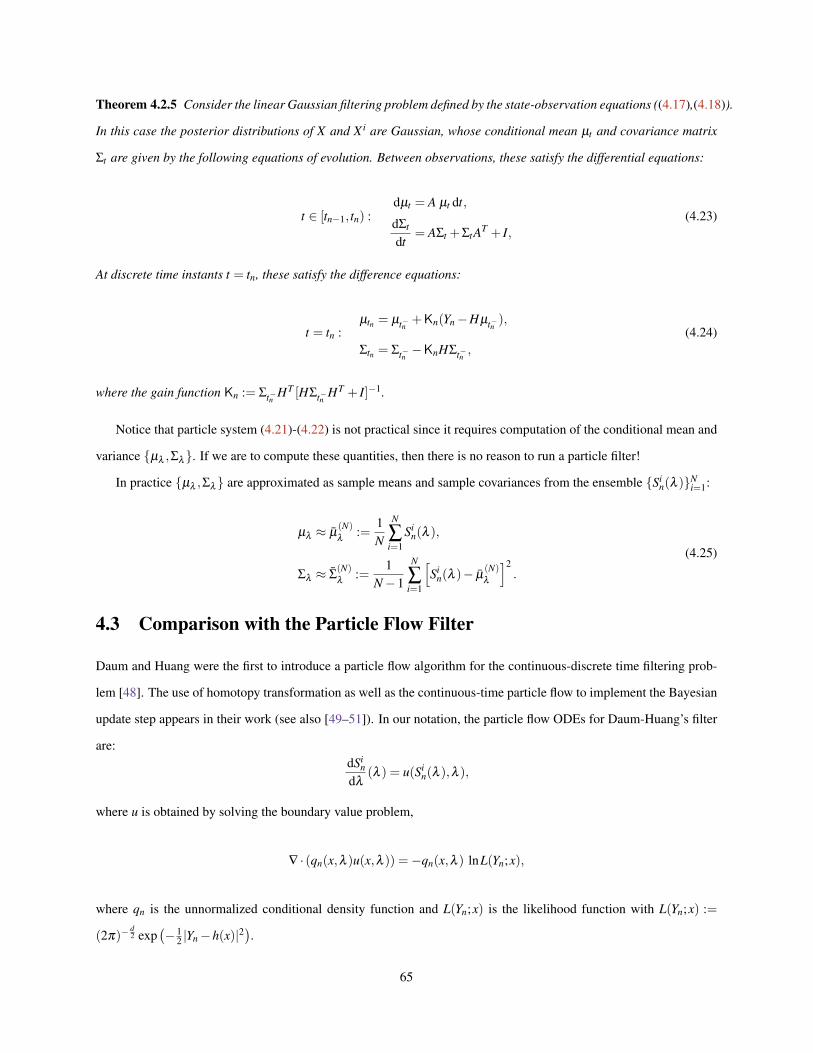
Theorem 4.2.5 Consider the linear Gaussian filtering problem defined by the state-observation equations ((4.17),(4.18)).
In this case the posterior distributions of X and X i are Gaussian, whose conditional mean µt and covariance matrix
Σt are given by the following equations of evolution. Between observations, these satisfy the differential equations:
t ∈ [tn−1, tn) :dµt = A µt dt,
dΣt
dt= AΣt +ΣtAT + I,
(4.23)
At discrete time instants t = tn, these satisfy the difference equations:
t = tn :µtn = µt−n +Kn(Yn−Hµt−n ),
Σtn = Σt−n −KnHΣt−n ,
(4.24)
where the gain function Kn := Σt−n HT [HΣt−n HT + I]−1.
Notice that particle system (4.21)-(4.22) is not practical since it requires computation of the conditional mean and
variance µλ ,Σλ. If we are to compute these quantities, then there is no reason to run a particle filter!
In practice µλ ,Σλ are approximated as sample means and sample covariances from the ensemble Sin(λ )N
i=1:
µλ ≈ µ(N)λ
:=1N
N
∑i=1
Sin(λ ),
Σλ ≈ Σ(N)λ
:=1
N−1
N
∑i=1
[Si
n(λ )− µ(N)λ
]2.
(4.25)
4.3 Comparison with the Particle Flow Filter
Daum and Huang were the first to introduce a particle flow algorithm for the continuous-discrete time filtering prob-
lem [48]. The use of homotopy transformation as well as the continuous-time particle flow to implement the Bayesian
update step appears in their work (see also [49–51]). In our notation, the particle flow ODEs for Daum-Huang’s filter
are:dSi
n
dλ(λ ) = u(Si
n(λ ),λ ),
where u is obtained by solving the boundary value problem,
∇ · (qn(x,λ )u(x,λ )) =−qn(x,λ ) lnL(Yn;x),
where qn is the unnormalized conditional density function and L(Yn;x) is the likelihood function with L(Yn;x) :=
(2π)−d2 exp
(− 1
2 |Yn−h(x)|2).
65
0 2 4 6 8 100
1FPF N=500FPF N=50KF
0 2 4 6 8 10
−1
0
1
FPF N=500FPF N=50KF
(a) (b)
Figure 4.2: Comparison of the Kalman filter and the feedback particle filter with different number of particles: (a)conditional mean; (b) conditional variance.
The main differences between the algorithm presented here and Daum-Huang’s filter concern
(i) the structure of the control law, and
(ii) the nature of the boundary value problems solved.
The innovation error-based gain feedback structure proposed here is motivated by the feedback particle filter algorithm
in continuous-time. The boundary value problems described in this chapter have a unique solution. This in particular
leads to a well-posed construction of the particle flow. Additional discussion of these issues for the continuous-time
problem appears in [154, 158].
4.4 Numerics
In this section, we provide numerical verification of the continuous-discrete feedback particle filter for a linear Gaus-
sian system. We provide comparisons with the classic continuous-discrete Kalman filter, which serves as a benchmark.
Consider the continuous-discrete time filtering problem:
dXt = A Xt dt +σB dBt ,
Yn = H Xtn +σW Wn,
where A = −0.5, H = 3, σB = 1, σW = 2, Bt is the standard Wiener process, Wn is the standard Gaussian white
noise, and Bt, Wn are mutually independent. Observations are available at tn = 0.5,1.0,1.5, . . . ,10.
The continuous-discrete feedback particle filter comprises of N particles where the controlled system of the i-th
66

0 2 4 6 8 10
−1
0
1
FPF
KF
0.01 .02 .05 0.1 .25 0.50
0.1
0.2
0.3
0.4
0.5
0.6
rmse
(a) (b)
Figure 4.3: (a). Comparison of true mean µt and estimated mean µ(N)t with ∆λ = 0.5; (b). Comparison of the rmse
with different choices of ∆λ .
particle is given by: For t ∈ [tn−1, tn),
dX it = A X i
t dt +σB dBit ,
and for t = tn,dSi
n
dλ(λ ) =
H Σ(N)λ
σ2W
[Yn−H
Sin(λ )+ µ
(N)λ
2
],
where λ ∈ [0,1] is the pseudo-time, Sin(0) := X i
t−n, and Bi
t are mutually independent standard Wiener processes. We
initialize the particle system by drawing initial conditions X i0N
i=1 from the distribution N(0,2). In the simulation
discussed next, the mean µ(N)λ
and the variance Σ(N)λ
are obtained from the ensemble Sin(λ )N
i=1 according to (4.25).
The total simulation time is T = 10, with real timestep ∆t = 0.05 and the pseudo timestep ∆λ = 0.05.
Fig. 4.2 summarizes some of the results of numerical experiments: Part (a) depicts the comparison of the true mean
µt obtained by Kalman filter and the estimated mean µ(N)t obtained using FPF with different number of particles.
Similarly, part (b) depicts the comparison of the true variance Σt and the estimated variance Σ(N)t . The true values of
µt and Σt are obtained by (4.23)-(4.24). It is seen that with N = 500 particles the continuous-discrete FPF approximates
the continuous-discrete Kalman filter quite well. With fewer particles (N = 50), the FPF performance degrades.
Fig. 4.3 depicts the result of a Monte Carlo study of the filter performance as the pseudo timestep ∆λ in Algo. 1 is
varied. Part (a) is a sample result using the same parameters as in Fig. 4.2-(a) but with ∆λ = 0.5. Part (b) depicts the
root mean square error (rmse) with different choices of ∆λ . The rmse is defined as:
rmse =
√1T
∫E[µ(N)t −µt
]2dt,
where the expectation is calculated over 100 Monte Carlo runs. As expected, the rmse increases as the discretization
∆λ gets coarser.
67
4.5 Conclusions
In this chapter, the feedback particle filter algorithm is generalized for the continuous-discrete time nonlinear filtering
problem. As with the continuous-time FPF, the continuous-discrete time algorithm i) admits an innovation error-based
feedback control structure, and ii) requires a solution of an E-L BVP. These solutions are described in closed-form
for the linear Gaussian filtering problem. For the general nonlinear non-Gaussian case, an algorithm is described to
obtain an approximate solution of the E-L BVP.
The purposes of studying the continuous-discrete time FPF algorithms are two-fold:
1. In many engineering and science applications, observations are only available at certain discrete time instances.
Therefore, a continuous-discrete time FPF algorithm is of practical value. The point is the proposed algorithm
retain the feedback control structure even for the nonlinear non-Gaussian case.
2. Comparisons are made to the continuous-discrete time particle flow filter algorithm introduced by Daum and
Huang [51]. It is shown that the FPF algorithm differs from the particle flow filter in both the structure of the
control law and the nature of the BVP solved.
68

Chapter 5
Feedback Particle Filter for aContinuous-Time Markov Chain∗
5.1 Introduction
In this chapter, we introduce the feedback particle filter to the continuous-time discrete-valued state-space nonlinear
filtering problem. Consider a Markov chain (Xt)t≥0 defined on a state-space comprising of standard basis in Rd :
e1,e2, . . . ,ed =: S. The chain is visualized as a directed graph whose edge, (l, l′), denotes possible transition from
state el ∈ S to another state el′ ∈ S/el . The set of all edges is denoted E.
Recall that a continuous time Markov chain with finite state-space can be realized using Poisson counters; cf., Chap. 2
of [32] for notation used in this chapter (see also [120] for a standard reference). The dynamics for the Markovian
state are given by,
dXt = ∑(l,l′)∈E
All′Xt dNll′t ,
where All′ := (el′ − el)⊗ el is a d × d matrix, and Nll′t denotes the state of a Poisson counter with rate λl′l . The
transition matrix for the Markov chain is then given by,
Λ = ∑(l,l′)∈E
λl′lAll′ .
The observation process is given by,
dZt = h(Xt)dt + dWt ,
where h : S→ R and Wt is a standard Wiener process.
The objective of the filtering problem is to compute or approximate the posterior distribution of Xt given the history
Zt := σ(Zs : 0≤ s≤ t). The posterior p∗t := (p∗(1, t), p∗(2, t), . . . , p∗(d, t))T is defined as,
p∗(l, t) = PXt = el |Zt, l = 1, . . . ,d. (5.1)
∗This chapter is an extension of the published paper [159].
69

Its evolution is described by the Wonham filter [148] (see (5.7)).
The objective of this chapter is to introduce a particle approximation of the Wonham filter. As in other particle
filtering techniques, the approximate filter is based on the construction of N stochastic processes X it : 1≤ i≤ N [7,
55, 74]. The value X it ∈ S is interpreted as the state for the ith particle at time t, and the empirical distribution is used
to approximate the conditional distribution. Recall that this is defined as,
pN(l, t) =1N
N
∑i=1
1lX it = el. (5.2)
The construction is as follows: The model for the ith particle is defined by a controlled system,
dX it = ∑
(l,l′)∈EAll′X i
t dNll′,it +
d
∑k=1
BkX it dC k,i
t︸ ︷︷ ︸Control
,
where Bk is a d×d matrix whose only non-zero entires are,
Bkll =−1 for l 6= k,
Bkkl = 1 for l 6= k
(5.3)
and C k,it denotes the state of a time-modulated Poisson counter of the following form: There is an input process Uk
t
and a family of mutually independent Poisson processes Nk,i( ·) with constant rate λ = 1, also independent of Zt
and Nll′,it , such that
C k,it = Nk,i(Uk
t ) , t ≥ 0.
The posterior distribution of X it given the history Z is denoted pt := (p(1, t), p(2, t), . . . , p(d, t))T , where
p(l, t) = PX it = el |Zt, l = 1, . . . ,d. (5.4)
The construction of the particle filter is reduced to a control problem: Choose the control input Ukt so that pt is equal
to p∗t , and consequently pNt (defined in (5.2)) approximates p∗t for large N. The main result of this chapter is the
solution of this control problem.
The solution is described as the stochastic differential equation driven by the observations and the particle evolu-
tion,
dUkt = K(k, t)(dZt − ht dt),
70
where ht := E[h(X it )|Zt ] = ∑
dl=1 hl p(l, t) and hl := h(el). In a numerical implementation, we approximate
ht ≈ hNt =
1N
N
∑i=1
h(X it ) .
The gain vector, Kt := (K(1, t),K(2, t), . . . ,K(d, t))T , is the solution of the following linear matrix problem,
(pt ⊗1− I)Kt =−(Ht − hI)pt ,
where 1 := (1,1, . . . ,1), I is the d×d identity matrix, and Ht := diag(h1, . . . ,hd).
The outline of the remainder of this chapter is as follows. The particle filter is introduced in Sec. 5.2, and shown to
be consistent with the Wonham filter. An algorithm to simulate the filter is discussed in Sec. 5.3, and illustrated with
a numerical example in Sec. 5.4.
5.2 Feedback Particle Filter for Markov Chains
The model for the particle filter is given by the stochastic differential equation,
dX it = ∑
(l,l′)∈EAll′X i
t dNll′,it +
d
∑k=1
BkX it dC k,i
t︸ ︷︷ ︸Control
, (5.5)
where X it ∈ S is the state for the ith particle at time t, and Nll′,i
t are mutually independent Poisson counters with rates
λl′l . We assume the initial conditions X i0N
i=1 are i.i.d., independent of Nll′,it , and drawn from the initial distribution
p∗(x,0) of X0. Both Nll′,it and X i
0 are also assumed to be independent of Xt ,Zt . The matrices All′ := (el′ − el)⊗ el
and Bk are the d×d matrices, as defined in Sec. 5.1 (see (5.3)).
For each particle, we introduce d-mutually independent time-modulated Poisson counters, denoted C k,it d
k=1. The
kth-counter jumps at times T k,i1 ,T k,i
2 , . . . ,T k,ij ,T k,i
j+1, . . . ,. The time between successive jumps, T k,ij+1−T k,i
j , is random.
Its law is defined by introducing a time-change process,
Ukt =
∫ t
0(K(k,s)dZs +u(k,s)ds) . (5.6)
In terms of this process, UT k,ij+1−UT k,i
j∼ exp(1). Introducing a family of mutually independent Poisson processes
Nk,i(·) with constant rate λ = 1, we have that:
C k,it = Nk,i(Uk
t ), t ≥ 0.
71

We impose admissibility requirements on the control input Ukt in (5.6):
Definition 4 (Admissible Input) The control input Ukt d
k=1 is admissible if the random variables
ut = (u(1, t),u(2, t), . . . ,u(d, t))T ,
Kt = (K(1, t),K(2, t), . . . ,K(d, t))T
are Zt measurable for each t. Moreover, at each t,
(i) Ukt is non-decreasing with probability one, and
(ii) E[‖ut‖+‖Kt‖]< ∞, where ‖ut‖2 = |u(1, t)|2 + · · ·+ |u(d, t)|2 and ‖Kt‖2 = |K(1, t)|2 + · · ·+ |K(d, t)|2.
The filtering problem is to define the control input in terms of ut ,Kt. We say that these functions are optimal if
pt ≡ p∗t , where recall
(i) pt is the posterior distribution of X it given Zt as defined in (5.4).
(ii) p∗t is the posterior distribution of Xt given Zt as defined in (5.1).
Given p∗(·,0) = p(·,0), our goal is to choose ut ,Kt in the feedback particle filter so that the evolution equations of
these conditional distributions coincide.
The evolution of p∗t is described by the Wonham filter:
dp∗t = Λp∗t dt +(Ht − hI)(dZt − hdt)p∗t . (5.7)
where Ht := diag(h1, . . . ,hd) and I denotes the identity matrix.
The evolution equation of pt is described next. The proof appears in App. D.1.
Proposition 5.2.1 Consider the process X it that evolves according to the particle filter model (5.5). The conditional
distribution of X it given the filtration Zt , pt , satisfies the forward equation
dpt = Λpt dt +(I− pt ⊗1)(Kt dZt +ut dt). (5.8)
5.2.1 Consistency with the Nonlinear Filter
The main result of this section is the construction of an optimal pair u,K.
72
The filter is obtained by comparing (5.7) with (5.8): the vector Kt = (K(1, t),K(2, t), . . . ,K(d, t))T is a solution of
(pt ⊗1− I)Kt =−(Ht − ht I)pt , (5.9)
and
u(k, t) =−K(k, t)ht .
With this choice of u,K, the control input is given by
Ukt =
∫ t
0K(k,s)(dZs− hs ds). (5.10)
The consideration of admissibility requires analysis of solutions of (5.9), described in the following proposition — Its
proof is given in App. D.2.
Proposition 5.2.2 Consider the problem (5.9). Its general solution is given by,
Kt = Ht pt + cpt , (5.11)
where c is an arbitrary constant. The minimal 2-norm solution is given by,
K0t = Ht pt + c0 pt ,
where c0 =−〈Ht pt , pt〉/‖pt‖2, 〈·, ·〉 denotes the standard inner product in Rd and ‖pt‖2 = 〈pt , pt〉.
For any solution Kt = (K(1, t), . . . ,K(d, t))T , the following property holds:
If p(k, t) = 0 then K(k, t) = 0. (P0)
Since 〈K0t , pt〉 = 0, necessarily, entires of K0
t can not all have one sign. This means that the control input Ukt
defined using Kt = K0t (see (5.10)) is not admissible. In order to obtain an admissible input, we use (5.11) to define
two particular solutions of (5.9):
K1t = K0
t + c1t pt , (5.12a)
K2t = K0
t + c2t pt , (5.12b)
where
73
(i) c1t is chosen so K1(k, t)≥ 0 for all k = 1, . . . ,d and mink K1(k, t) = 0.
(ii) c2t is chosen so K2(k, t)≤ 0 for all k = 1, . . . ,d and maxk K2(k, t) = 0.
The constants c1t ,c
2t exist because of property (P0).
Using solutions (5.12a)-(5.12b) we define an index vector Is, taking values in 1,2, such that
Ukt =
∫ t
0KIs(k,s)(dZs− hs ds) (5.13)
is a non-decreasing function of time. The control input defined using (5.13) is admissible by construction – the
instantaneous rate of the slowest counter is zero, and the rates of the remaining counters is non-negative. Moreover,
the gain function has minimal 2-norm at each time.
The following theorem shows that the two evolution equations (5.7) and (5.8) are identical. The proof is straight-
forward by direct comparison and thus omitted.
Theorem 5.2.3 Consider the two evolution equations for pt and p∗t , defined according to the solution of the forward
equation (5.8) and the Wonham filter (5.7), respectively. Suppose that the control input is obtained according to (5.13).
Then, provided p(·,0) = p∗(·,0), we have for all t ≥ 0,
p(·, t) = p∗(·, t).
5.3 Algorithm
In this section, we summarize a practical algorithm for simulating the proposed particle filter. We begin by describing
an algorithm for simulating Poisson counters with time-dependent rate.
5.3.1 Poisson Counter with Time-Dependent Rate
In order to implement the particle filter (5.5), we need to sample Poisson counter with time-dependent rates.
Consider a Poisson counter Ct where the counter jumps at times T1,T2, . . . ,Tj,Tj+1, . . .. The time between
successive jumps, Tj+1−Tj, is random and its law is governed by a time-change process:
Ut =∫ t
0dλs, (5.14)
where λt is a given time-dependent rate. In term of this process, UTj+1 −UTj ∼ exp(1).
74
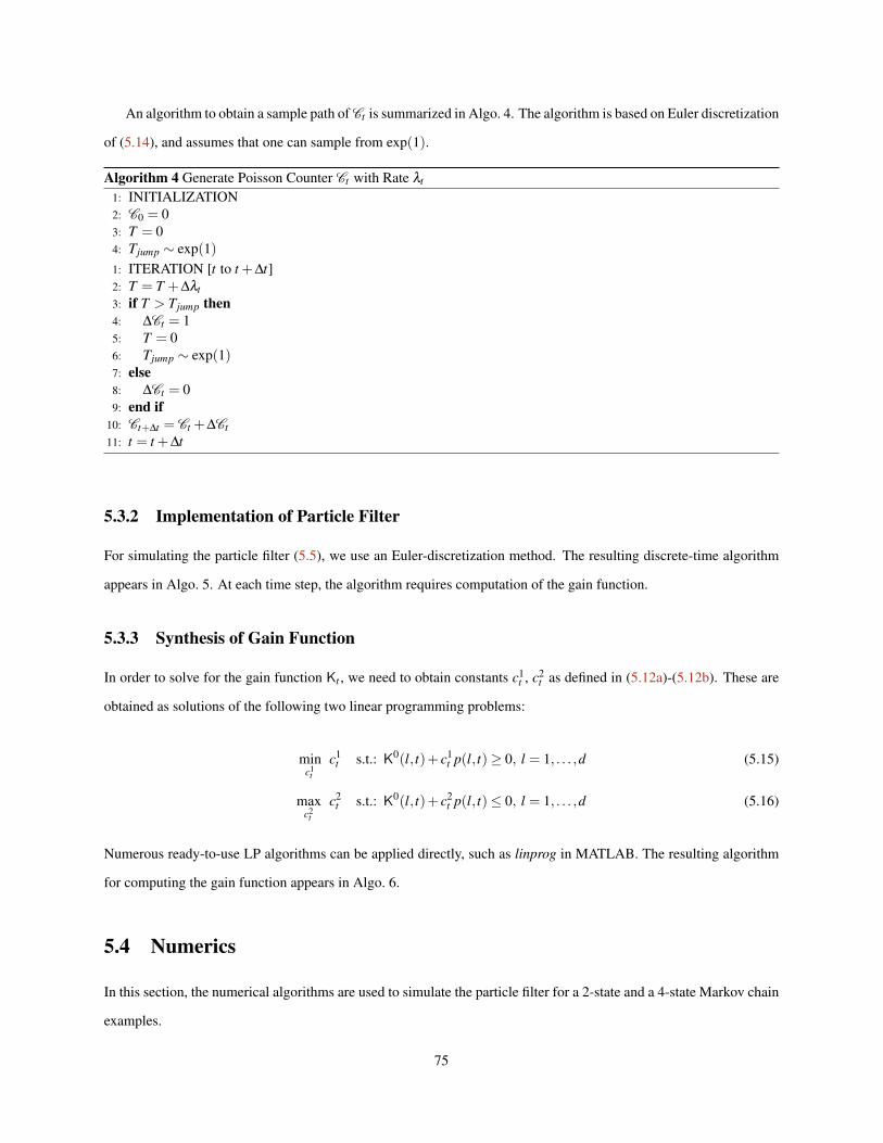
An algorithm to obtain a sample path of Ct is summarized in Algo. 4. The algorithm is based on Euler discretization
of (5.14), and assumes that one can sample from exp(1).
Algorithm 4 Generate Poisson Counter Ct with Rate λt
1: INITIALIZATION2: C0 = 03: T = 04: Tjump ∼ exp(1)1: ITERATION [t to t +∆t]2: T = T +∆λt3: if T > Tjump then4: ∆Ct = 15: T = 06: Tjump ∼ exp(1)7: else8: ∆Ct = 09: end if
10: Ct+∆t = Ct +∆Ct11: t = t +∆t
5.3.2 Implementation of Particle Filter
For simulating the particle filter (5.5), we use an Euler-discretization method. The resulting discrete-time algorithm
appears in Algo. 5. At each time step, the algorithm requires computation of the gain function.
5.3.3 Synthesis of Gain Function
In order to solve for the gain function Kt , we need to obtain constants c1t , c2
t as defined in (5.12a)-(5.12b). These are
obtained as solutions of the following two linear programming problems:
minc1
t
c1t s.t.: K0(l, t)+ c1
t p(l, t)≥ 0, l = 1, . . . ,d (5.15)
maxc2
t
c2t s.t.: K0(l, t)+ c2
t p(l, t)≤ 0, l = 1, . . . ,d (5.16)
Numerous ready-to-use LP algorithms can be applied directly, such as linprog in MATLAB. The resulting algorithm
for computing the gain function appears in Algo. 6.
5.4 Numerics
In this section, the numerical algorithms are used to simulate the particle filter for a 2-state and a 4-state Markov chain
examples.
75
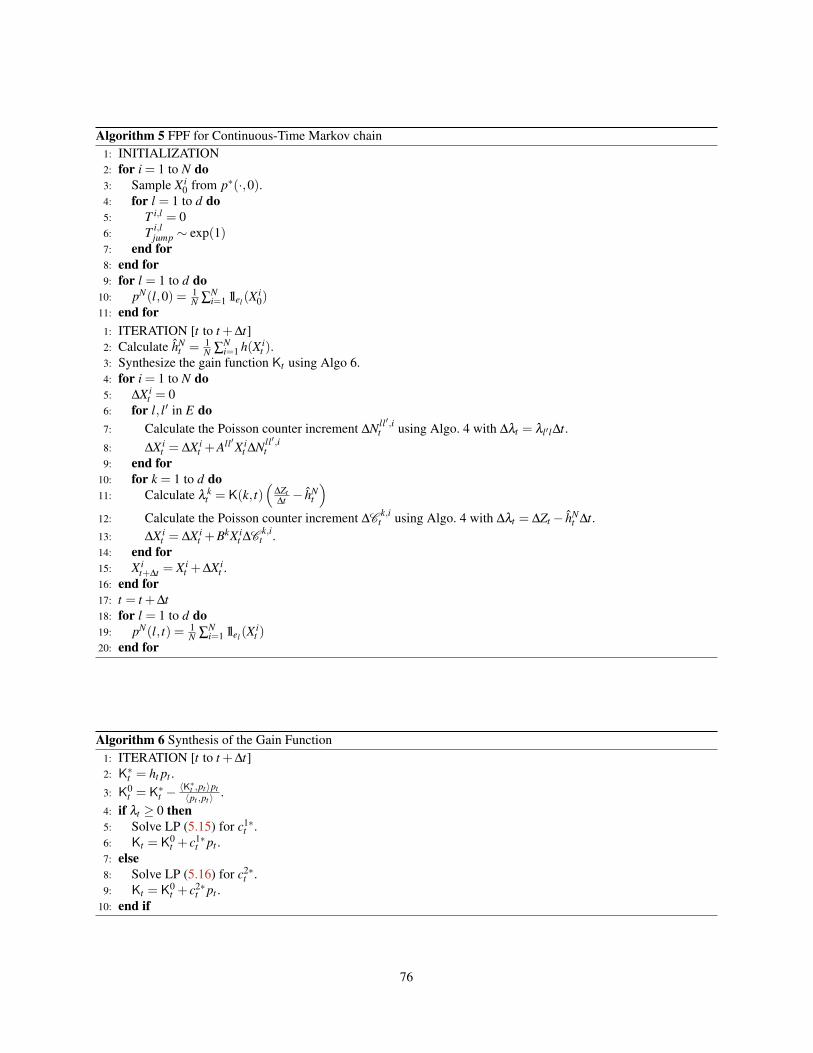
Algorithm 5 FPF for Continuous-Time Markov chain1: INITIALIZATION2: for i = 1 to N do3: Sample X i
0 from p∗(·,0).4: for l = 1 to d do5: T i,l = 06: T i,l
jump ∼ exp(1)7: end for8: end for9: for l = 1 to d do
10: pN(l,0) = 1N ∑
Ni=1 1lel (X
i0)
11: end for1: ITERATION [t to t +∆t]2: Calculate hN
t = 1N ∑
Ni=1 h(X i
t ).3: Synthesize the gain function Kt using Algo 6.4: for i = 1 to N do5: ∆X i
t = 06: for l, l′ in E do7: Calculate the Poisson counter increment ∆Nll′,i
t using Algo. 4 with ∆λt = λl′l∆t.8: ∆X i
t = ∆X it +All′X i
t ∆Nll′,it
9: end for10: for k = 1 to d do11: Calculate λ k
t = K(k, t)(
∆Zt∆t − hN
t
)12: Calculate the Poisson counter increment ∆C k,i
t using Algo. 4 with ∆λt = ∆Zt − hNt ∆t.
13: ∆X it = ∆X i
t +BkX it ∆C k,i
t .14: end for15: X i
t+∆t = X it +∆X i
t .16: end for17: t = t +∆t18: for l = 1 to d do19: pN(l, t) = 1
N ∑Ni=1 1lel (X
it )
20: end for
Algorithm 6 Synthesis of the Gain Function1: ITERATION [t to t +∆t]2: K∗t = ht pt .3: K0
t = K∗t − 〈K∗t ,pt 〉pt〈pt ,pt 〉 .
4: if λt ≥ 0 then5: Solve LP (5.15) for c1∗
t .6: Kt = K0
t + c1∗t pt .
7: else8: Solve LP (5.16) for c2∗
t .9: Kt = K0
t + c2∗t pt .
10: end if
76
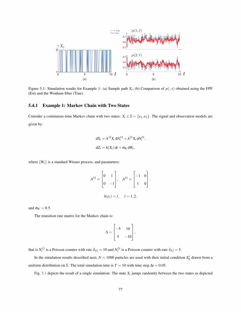
0.5
0.6
0.7
0.3
0.4
0.5
0 5 10 0 5 101
2
(a) (b)
TrueEst.
Figure 5.1: Simulation results for Example 1: (a) Sample path Xt ; (b) Comparison of p(·, t) obtained using the FPF(Est) and the Wonham filter (True).
5.4.1 Example 1: Markov Chain with Two States
Consider a continuous-time Markov chain with two states: Xt ∈ S= e1,e2. The signal and observation models are
given by:
dXt = A12Xt dN12t +A21Xt dN21
t ,
dZt = h(Xt)dt +σW dWt ,
where Wt is a standard Wiener process, and parameters:
A12 =
0 1
0 −1
, A21 =
−1 0
1 0
,h(el) = l, l = 1,2.
and σW = 0.5.
The transition rate matrix for the Markov chain is:
Λ =
−5 10
5 −10
,that is N12
t is a Poisson counter with rate λ21 = 10 and N21t is a Poisson counter with rate λ12 = 5.
In the simulation results described next, N = 1000 particles are used with their initial condition X i0 drawn from a
uniform distribution on S. The total simulation time is T = 10 with time step ∆t = 0.05.
Fig. 5.1 depicts the result of a single simulation: The state Xt jumps randomly between the two states as depicted
77
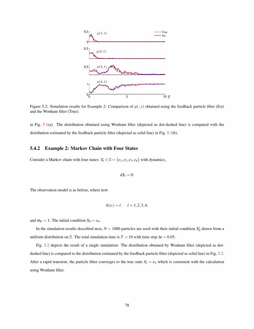
0
0.5
0.5
0.5
0
1
TrueEst.
0 5 10
Figure 5.2: Simulation results for Example 2: Comparison of p(·, t) obtained using the feedback particle filter (Est)and the Wonham filter (True).
in Fig. 5.1(a). The distribution obtained using Wonham filter (depicted as dot-dashed line) is compared with the
distribution estimated by the feedback particle filter (depicted as solid line) in Fig. 5.1(b).
5.4.2 Example 2: Markov Chain with Four States
Consider a Markov chain with four states: Xt ∈ S= e1,e2,e3,e4 with dynamics,
dXt = 0.
The observation model is as before, where now
h(el) = l, l = 1,2,3,4,
and σW = 1. The initial condition X0 = e4.
In the simulation results described next, N = 1000 particles are used with their initial condition X i0 drawn from a
uniform distribution on S. The total simulation time is T = 10 with time step ∆t = 0.05.
Fig. 5.2 depicts the result of a single simulation: The distribution obtained by Wonham filter (depicted as dot-
dashed line) is compared to the distribution estimated by the feedback particle filter (depicted as solid line) in Fig. 5.2.
After a rapid transient, the particle filter converges to the true state Xt = e4 which is consistent with the calculation
using Wonham filter.
78

5.5 Conclusions
In this chapter, we introduced a feedback particle filter algorithm for approximation of the Wonham filter. The control
is realized using Poisson processes. The algorithm is expected to be useful in certain applications:
1. A single Poisson process serves as a reduced order model of the firing of a single neuron [33, 43]. Given the
importance of the Bayesian inference paradigm in neuroscience (cf., [58, 105]), the algorithm can be used to
develop specific neuromorphic implementations.
2. In problems involving estimation of maneuvering targets, continuous time Markov chains are used to model
target maneuvers [10, 19]. The algorithm described here is seen as an intermediate step towards developing
particle filter algorithms for such problems.
Both these applications are subject of the ongoing work.
79

Part II
Applications
80

Chapter 6
Interacting Multiple Model-FeedbackParticle Filter∗
6.1 Introduction
In many applications, including air and missile defense systems, remote sensing, autonomous navigation and robotics,
additional model uncertainty might enter the system besides the uncertainty associated with signal and observation
noise [10]. The uncertainty is typically modeled using a stochastic hybrid system (SHS) framework. Treating the
model uncertainty as a discrete variable in the augmented state space, the SHS filtering problem involves the estimation
of a partially observed stochastic process with both continuous-valued and discrete-valued states.
An example is to track a maneuvering target (hidden signal) with noisy radar measurements. In this case, the SHS
is comprised of the continuous-valued states which represent target positions and velocities, and the discrete-valued
states which represent the distinct dynamic model types (e.g., constant velocity or white noise acceleration model) of
the target. The discrete signal model types are referred to as modes. Since the time of target maneuvers is random,
there is model uncertainty in the sense that one can not assume, in an apriori fashion, a fixed dynamic model of the
target.
Motivated in part by target tracking applications, we consider models of SHS where the continuous-valued state
process is modeled using a stochastic differential equation (SDE), and the discrete-valued state process is modeled as
a continuous-time Markov chain. The estimation objective is to estimate (filter) the hidden states (both continuous-
and discrete-valued state) given noisy observations.
Given the number of applications, algorithms for SHS filtering problems have been extensively studied in the past;
cf., [10, 112] and references therein. A typical SHS filtering algorithm is comprised of three parts:
(i) A filtering algorithm to estimate the continuous-valued state given the mode,
(ii) An association algorithm to associate modes to signal dynamics,
(iii) A merging process to combine the results of i) and ii).
Prior to mid-1990s, the primary tool for filtering was a Kalman filter or one of its extensions, e.g., extended∗This chapter is an extension of the published paper [151].
81
Kalman filter. The limitations of these tools in applications arise on account of nonlinearities, not only in dynamic
motion of targets (e.g., drag forces in ballistic targets) but also in the measurement models (e.g., range or bearing).
The nonlinearities can lead to a non-Gaussian multimodal conditional distribution. For such cases, Kalman and
extended Kalman filters are known to perform poorly; cf., [132]. Since the advent and wide-spread use of particle
filters [55], such filters are becoming increasingly relevant to SHS estimation for target tracking applications; cf., [132]
and references therein.
The other part is the mode association algorithm. The purpose of the mode association algorithm is to determine
the conditional probability for the discrete modes.
In a discrete-time setting, the exact solution to problems (i)-(iii) is given by a Multiple Model (MM) filter which
has an (exponentially with time) increasing number of filters, one for each possible mode history. Practically, however,
the number of filters has to be limited, which leads to the classical Generalised Pseudo-Bayes estimators of the first
and second order (GPB1 and GPB2) and the Interacting Multiple Model (IMM) filter [10]. For some SHS examples,
however, it was already shown in [21] that these low-dimensional filters do not always perform well. This has led to
the development of two types of particle filters for SHS:
(i) The first approach is to apply the standard particle filtering approach to the joint continuous-valued state and
discrete-valued mode process [113], [119].
(ii) The second approach is to exploit Rao-Blackwellization, in the sense of applying particle filtering for the continuous-
valued state, and exact filter recursions for the discrete-valued modes [59], [26], [28].
In this chapter, we consider a continuous-time filtering problem for SHS and develop a feedback control-based
particle filter algorithm, where the particles represent continuous-valued state components (case (ii)). We refer to the
resulting algorithm as the Interacting Multiple Model-Feedback Particle Filter (IMM-FPF). As the name suggests, the
proposed algorithm represents a generalization of the Kalman filter-based IMM algorithm to the general nonlinear
filtering problem.
One remarkable conclusion is that the IMM-FPF retains the innovation error-based feedback structure even for
the nonlinear problem. The interaction/merging process is also handled via a control-based approach. The innovation
error-based feedback structure is expected to be useful because of the coupled nature of the filtering and the mode
association problem. The theoretical results are illustrated with a numerical example.
The outline of the remainder of this chapter is as follows: The exact filtering equations appear in Sec. 6.2. The
IMM-FPF is introduced in Sec. 6.3 and the numerical example is described in Sec. 6.4.
82
6.2 Problem Formulation and Exact Filtering Equations
In this section, we formulate the continuous-time SHS filtering problem, introduce the notation, and summarize the
exact filtering equations (see [20, 108] for standard references). For pedagogical reason, we limit the considerations
to scalar-valued signal and observation processes. The generalization to multivariable case is straightforward.
6.2.1 Problem Statement, Assumptions and Notation
The following notation is adopted:
(i) At time t, the signal state is denoted by Xt ∈ R.
(ii) At time t, the mode random variable is denoted as θt , defined on a state-space comprising of the standard basis in
RM: e1,e2, . . . ,eM =: S. It associates a specific mode to the signal: θt = em signifies that the dynamics at time t
is described by the mth model.
(iii) At time t, there is only one observation Zt ∈ R. The observation history (filtration) is denoted as Z := σ(Zs : 0 ≤
s≤ t).
The following models are assumed for the three stochastic processes:
(i) The evolution of the continuous-valued state Xt is described by a stochastic differential equation with discrete-valued
coefficients:
dXt = a(Xt ,θt)dt +σ(θt)dBt , (6.1)
where Bt is a standard Wiener process. We denote am(x) := a(x,em) and σm := σ(em).
(ii) The discrete-valued state (mode) θt evolves as a Markov chain in continuous-time:
P(θt+δ = el |θt = em) = qmlδ +o(δ ), m 6= l. (6.2)
The generator for this jump process is denoted by a stochastic matrix Q whose mlth entry is qml for m 6= l. The
initial distribution is assumed to be given.
(iii) At time t, the observation model is given by,
dZt = h(Xt ,θt)dt + dWt , (6.3)
where Wt is a standard Wiener process assumed to be independent of Bt. We denote hm(x) := h(x,em).
The filtering problem is to obtain the posterior distribution of Xt given Z .
83
6.2.2 Exact Filtering Equations
The following distributions are of interest:
(i) q∗m(x, t) defines the joint conditional distribution of (Xt ,θt)T given Zt , i.e.,
∫x∈A
q∗m(x, t)dx = P[Xt ∈ A,θt = em]|Z ,
for A ∈B(R) and m ∈ 1, . . . ,M. We denote q∗(x, t) := (q∗1(x, t),q∗2(x, t), . . . ,q
∗M(x, t))T , interpreted as a column
vector.
(ii) p∗(x, t) defines the conditional dist. of Xt given Z :
∫x∈A
p∗(x, t)dx = PXt ∈ A|Z , A ∈B(R).
By definition, we have p∗(x, t) = ∑Mm=1 q∗m(x, t).
(iii) µt := (µ1t , . . . ,µ
Mt )T defines the probability mass function of θt given Z where:
µmt = Pθt = em|Z , m = 1, . . . ,M. (6.4)
By definition µmt =
∫R q∗m(x, t)dx.
(iv) ρ∗m(x, t) defines the conditional dist. of Xt given θt = em and Z . For µmt 6= 0:
ρ∗m(x, t) :=
q∗m(x, t)µm
t, m = 1, . . . ,M, (6.5)
Denote ρ∗(x, t) = (ρ∗1 (x, t), . . . ,ρ∗M(x, t))T .
We introduce two more notations before presenting the exact filtering equations for these density functions:
(i) ht := E[h(Xt ,θt)|Z ] = ∑Mm=1
∫R hm(x)q∗m(x, t)dx;
(ii) hmt := E[h(Xt ,θt)|θt = em,Z ] =
∫R hm(x)ρ∗m(x, t)dx.
Note that ht = ∑Mm=1 µm
t hmt .
The following theorem describes the evolution of above-mentioned density functions. A short proof is included
in App. E.1.
Theorem 6.2.1 (See also Theorem 1 in [20]) Consider the hybrid system (6.1) - (6.3):
84
(i) The joint conditional distribution of (Xt ,θt)T satisfies:
dq∗ = L †(q∗)dt +QT q∗ dt +(Ht − ht I)(dZt − ht dt)q∗, (6.6)
where L † = diagL †m, Ht = diaghm, I is an M×M identity matrix and
L †mq∗m :=− ∂
∂x(amq∗m)+
12(σm)2 ∂ 2
∂x2 q∗m.
(ii) The conditional distribution of θt satisfies:
dµt = QTµt dt +(Ht − ht I)(dZt − ht dt)µt , (6.7)
where Ht = diaghmt .
(iii) The conditional distribution of Xt satisfies:
dp∗ =M
∑m=1
L †m(q
∗m)dt +
M
∑m=1
(hm− ht)(dZt − ht dt)q∗m. (6.8)
(iv) The conditional distribution of Xt given θt = em satisfies:
dρ∗m = L †
mρ∗m dt +
1µm
t
M
∑l=1
qlmµlt (ρ∗l −ρ
∗m)dt +(hm− hm
t )(dZt − hmt dt)ρ∗m, m = 1, . . . ,M (6.9)
6.3 IMM-Feedback Particle Filter
The IMM-FPF is comprised of M parallel feedback particle filters: The model for the mth particle filter is,
dX i;mt = am(X i;m
t )dt +σm dBi;m
t + dU i;mt , (6.10)
where X i;mt ∈ R is the state for the ith particle at time t, U i;m
t is its control input, Bi;mt N
i=1 are mutually independent
standard Wiener processes and N denotes the number of particles. We assume that the initial conditions X i;m0 N
i=1
are i.i.d., independent of Bi;mt , and drawn from the initial distribution ρ∗m(x,0) of X0. Both Bi;m
t and X i;m0 are
assumed to be independent of both Xt and Zt . Certain additional assumptions are made regarding admissible forms of
control input (see [154]).
Remark 7 The motivation for choosing the parallel structure comes from the conventional IMM filter, which is com-
85
prised of M parallel Kalman filters, one for each maneuvering mode m ∈ 1, . . . ,M. ut
There are two types of conditional distributions of interest in our analysis:
(i) ρ∗m(x, t): Defines the conditional dist. of Xt given θt = em and Z , see (6.5).
(ii) ρm(x, t): Defines the conditional dist. of X i;mt given Z :
∫x∈A
ρm(x, t)dx = PX i;mt ∈ A|Z , ∀A ∈B(R).
The control problem is to choose the control inputs U i;mt M
m=1 so that, ρm approximates ρ∗m for each m = 1, . . . ,M.
Consequently the empirical distribution of the particles approximates ρ∗m for large number of particles [153].
The main result of this section is to describe an explicit formula for the optimal control input, and demonstrate
that under general conditions we obtain an exact match: ρm = ρ∗m, under optimal control. The optimally controlled
dynamics of the ith particle in the mth FPF have the following Stratonovich form,
dX i;mt = am(X i;m
t )dt +σm dBi;m
t +Km(X i;mt , t) dIi;m
t +um(X i;mt ,X i;−m
t , t)dt, (6.11)
where X i;−mt = X i;l
t l 6=m and Ii;mt is the modified form of innovation process,
dIi;mt := dZt −
12
[hm(X i;m
t )+ hmt
]dt, (6.12)
where hmt :=
∫R hm(x)ρm(x, t)dx. The gain function Km is obtained as a solution of an Euler-Lagrange boundary value
problem (E-L BVP):∂ (ρmKm)
∂x=−(hm− hm
t )ρm, (6.13)
with boundary condition limx→±∞ ρm(x, t)Km(x, t) = 0.
The interaction between filters arises as a result of the control term um. It is obtained by solving the following
BVP:∂ (ρmum)
∂x=
M
∑l=1
clm(ρm−ρl), (6.14)
again with boundary condition limx→±∞ ρm(x, t)um(x, t) = 0 and clm := qlmµ lt
µmt
.
Recall that the evolution of ρ∗m(x, t) is described by the modified Kushner-Stratonovich (K-S) equation (6.9). The
evolution of ρm is given by a forward Kolmogorov operator (derived in App. E.2).
The following theorem shows that the evolution equations for ρm and ρ∗m are identical. The proof appears in
App. E.2.
86
Theorem 6.3.1 Consider the two distributions ρm and ρ∗m. Suppose that, for m = 1, . . . ,M, the gain function Km(x, t)
and the control term um is obtained according to (6.13) and (6.14), respectively. Then provided ρm(x,0) = ρ∗m(x,0),
we have for all t > 0, ρm(x, t) = ρ∗m(x, t).
In a numerical implementation, one also needs to estimate µmt , which is done by using the same finite-dimensional
filter, as in (6.7):
dµmt =
M
∑l=1
qlmµlt dt +(hm
t − ht)(dZt − ht dt)µmt , (6.15)
where ht = ∑Mm=1 µm
t hmt and hm
t ≈ 1N ∑
Ni=1 hm(X i;m
t ) are approximated with particles.
Remark 8 The mode association probability filter (6.15) can also be derived by considering a continuous-time limit
starting from the continuous-discrete time filter that appears in the classic IMM filter literature [10]. This proof
appears in App. E.3. The alternate proof is included because it shows that the filter (6.15) is in fact the continuous-time
nonlinear counterpart of the algorithm that is used to obtain association probability in the classical IMM literature.
The proof also suggests alternate discrete-time algorithms for evaluating association probabilities in simulations and
experiments, where observations are made at discrete sampling times.
Define p(x, t) := ∑Mm=1 µm
t ρm(x, t) where µmt is defined in (6.4). The following corollary shows that p(x, t) and
p∗(x, t) are identical. Its proof is straightforward, by using the definitions, and is thus omitted.
Corollary 6.3.1 Consider the two distribution p(x, t) and p∗(x, t). Suppose conditions in Thm. 6.3.1 apply, and µmt is
obtained using (6.15), then provided p(x,0) = p∗(x,0), we have for all t > 0, p(x, t) = p∗(x, t).
6.3.1 Algorithm
The main difficulty is to obtain a solution of the BVP (6.13) and (6.14) at each time step. A Galerkin algorithm for
the same appears in our earlier paper [154]. One particular approximation of the solution, referred to as the constant
gain approximation is given by:
Km ≈ 1N
N
∑i=1
(hm(X i;mt )− hm
t )Xi;mt , (6.16)
um ≈M
∑l=1
clm1N
(N
∑i=1
X i;lt −
N
∑i=1
X i;mt
), (6.17)
which is constant at each given time. The justification of the constant approximation appears in our earlier paper [154].
Apart from the gain function, the algorithm requires approximation of ht and hmt . These are obtained in terms of
87

particles as:
hmt ≈
1N
N
∑i=1
hm(X i;mt ), ht =
M
∑m=1
µmt hm
t .
For simulating the IMM-FPF, we use an Euler-discretization method. The resulting discrete-time algorithm appears
in Algo.7. At each time step, the algorithm requires computation of the gain function, that is obtained using (6.16)-
(6.17).
Algorithm 7 IMM-FPF for SHS1: INITIALIZATION2: for m = 1 to M do3: µm
0 = 1M .
4: for i = 1 to N do5: Sample X i;m
0 from p∗(·,0).6: end for7: end for1: ITERATION [t to t +∆t]2: for m = 1 to M do3: Calculate hm
t ≈ 1N ∑
Ni=1 hm(X i;m
t ).4: end for5: Calculate ht = ∑
Mm=1 µm
t hmt .
6: for m = 1 to M do7: for i = 1 to N do8: Generate a sample, ∆V , from N(0,1)9: Calculate ∆Ii;m
t = ∆Zt − 12
[hm(X i;m
t )+ hmt
]∆t
10: Calculate the gain function Km (e.g., by using (6.16))11: Calculate the control term um (e.g., by using (6.17)).12: ∆X i;m
t = am(X i;mt )∆t +σm
√∆t∆V +Km∆Ii;m
t +um∆t13: X i;m
t+∆t = X i;mt +∆X i;m
t14: end for15: µm
t+∆t = µmt +∑
Ml=1 qlmµ l
t ∆t +(hmt − ht)(∆Zt − ht∆t)µm
t .16: end for17: t = t +∆t18: Xt := E[Xt |Z ]≈ 1
N ∑Mm=1 ∑
Ni=1 µm
t X i;mt .
88
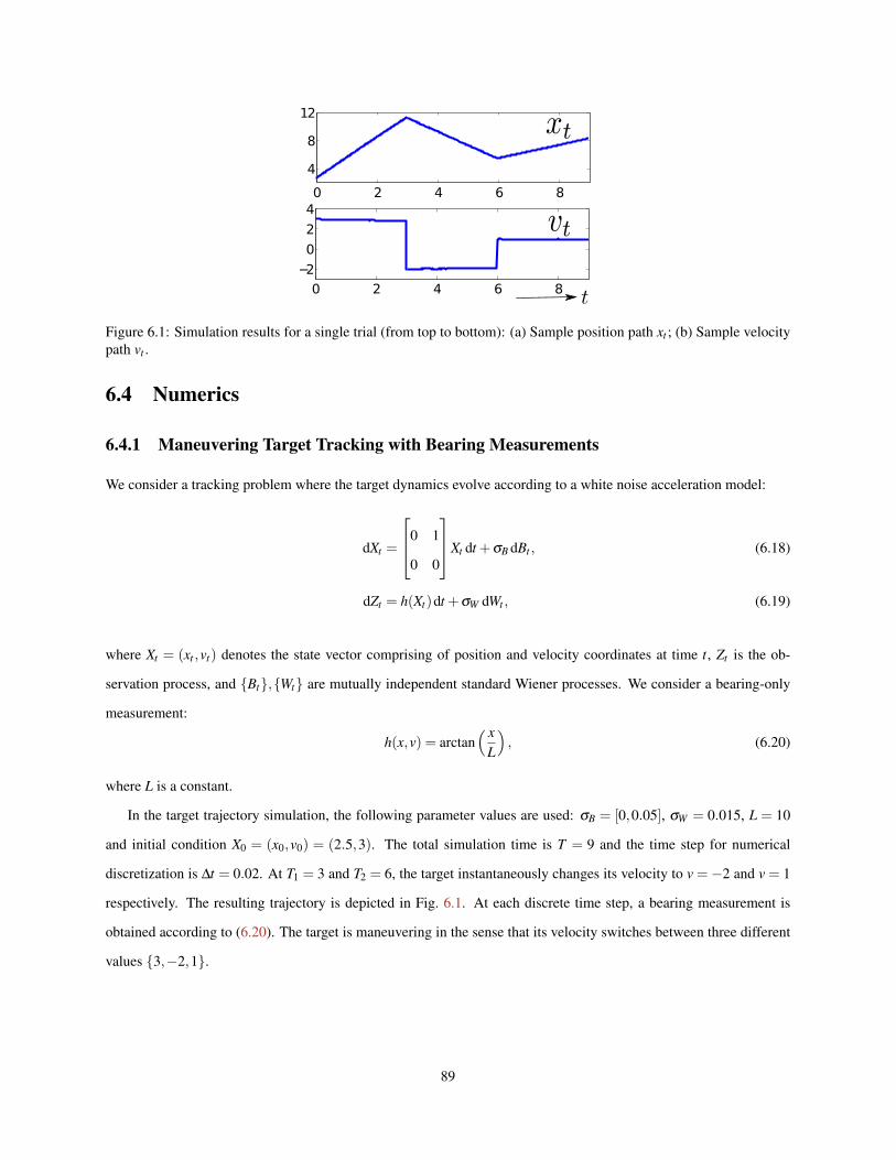
0 2 4 6 8
4
8
12
0 2 4 6 8
−2
0
2
4
Figure 6.1: Simulation results for a single trial (from top to bottom): (a) Sample position path xt ; (b) Sample velocitypath vt .
6.4 Numerics
6.4.1 Maneuvering Target Tracking with Bearing Measurements
We consider a tracking problem where the target dynamics evolve according to a white noise acceleration model:
dXt =
0 1
0 0
Xt dt +σB dBt , (6.18)
dZt = h(Xt)dt +σW dWt , (6.19)
where Xt = (xt ,vt) denotes the state vector comprising of position and velocity coordinates at time t, Zt is the ob-
servation process, and Bt,Wt are mutually independent standard Wiener processes. We consider a bearing-only
measurement:
h(x,v) = arctan( x
L
), (6.20)
where L is a constant.
In the target trajectory simulation, the following parameter values are used: σB = [0,0.05], σW = 0.015, L = 10
and initial condition X0 = (x0,v0) = (2.5,3). The total simulation time is T = 9 and the time step for numerical
discretization is ∆t = 0.02. At T1 = 3 and T2 = 6, the target instantaneously changes its velocity to v =−2 and v = 1
respectively. The resulting trajectory is depicted in Fig. 6.1. At each discrete time step, a bearing measurement is
obtained according to (6.20). The target is maneuvering in the sense that its velocity switches between three different
values 3,−2,1.
89
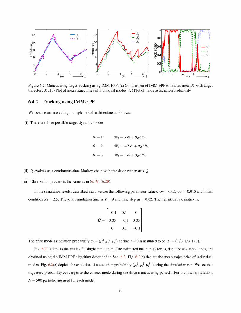
0 2 4 6 82
4
6
8
10
12Position
(a)0 2 4 6 82
4
6
8
10
12
Position
(b)0 2 4 6 80
0.2
0.4
0.6
0.8
1
Probability
(c)
Figure 6.2: Maneuvering target tracking using IMM-FPF: (a) Comparison of IMM-FPF estimated mean Xt with targettrajectory Xt . (b) Plot of mean trajectories of individual modes. (c) Plot of mode association probability.
6.4.2 Tracking using IMM-FPF
We assume an interacting multiple model architecture as follows:
(i) There are three possible target dynamic modes:
θt = 1 : dXt = 3 dt +σB dBt ,
θt = 2 : dXt =−2 dt +σB dBt ,
θt = 3 : dXt = 1 dt +σB dBt .
(ii) θt evolves as a continuous-time Markov chain with transition rate matrix Q.
(iii) Observation process is the same as in (6.19)-(6.20).
In the simulation results described next, we use the following parameter values: σB = 0.05, σW = 0.015 and initial
condition X0 = 2.5. The total simulation time is T = 9 and time step ∆t = 0.02. The transition rate matrix is,
Q =
−0.1 0.1 0
0.05 −0.1 0.05
0 0.1 −0.1
The prior mode association probability µt = (µ1
t ,µ2t ,µ
3t ) at time t = 0 is assumed to be µ0 = (1/3,1/3,1/3).
Fig. 6.2(a) depicts the result of a single simulation: The estimated mean trajectories, depicted as dashed lines, are
obtained using the IMM-FPF algorithm described in Sec. 6.3. Fig. 6.2(b) depicts the mean trajectories of individual
modes. Fig. 6.2(c) depicts the evolution of association probability (µ1t ,µ
2t ,µ
3t ) during the simulation run. We see that
trajectory probability converges to the correct mode during the three maneuvering periods. For the filter simulation,
N = 500 particles are used for each mode.
90

6.5 Conclusions
In this chapter, we introduced a feedback particle filter-based algorithm for the filtering problem with model un-
certainty. The additional uncertainty is modeled in a continuous-time SHS framework. The proposed algorithm is
shown to be the nonlinear generalization of the conventional Kalman filter-based IMM algorithm. One remarkable
conclusion is that the IMM-FPF solution retains the innovation error-based feedback structure even for the nonlinear
non-Gaussian case. The interaction/merging process is also handled via a control-based approach. The theoretical
results are illustrated with the aid of a numerical example problem from a maneuvering target tracking application.
The ongoing research concerns the following two topics:
(i) Comparison of the IMM-FPF algorithm against the basic particle filter (PF) and the IMM-PF, with respect to esti-
mation accuracy and computational burden.
(ii) Investigation of alternate FPF-based algorithms for SHS estimation. Of particular interest is the filter architecture
where particles evolve in the joint state space (analogous to case (i) in Sec. 6.1).
91

Chapter 7
Probabilistic Data Association-FeedbackParticle Filter∗
7.1 Introduction
Filtering with data association uncertainty is important to a number of applications, including, air and missile de-
fense systems, air traffic surveillance, weather surveillance, ground mapping, geophysical surveys, remote sensing,
autonomous navigation and robotics [8, 137]. One example is the problem of multiple target tracking (MTT) with
radar observations. The targets can be multiple aircrafts in air defense, multiple ballistic objects in missile defense,
multiple weather cells in weather surveillance, or multiple landmarks in autonomous navigation and robotics. In each
of these applications, there exists data association uncertainty in the sense that one can not assign, in an apriori manner,
individual observations (measurements) to individual targets.
Given the large number of applications, algorithms for filtering problems with data association uncertainty have
been extensively studied in the past; cf., [8, 97, 101, 124] and references therein. A typical algorithm is comprised of
two parts:
(i) A filtering algorithm for tracking a single target, and
(ii) A data association algorithm for associating observations to targets.
Various filtering algorithms have been proposed for the first part, including the classical Kalman filter-based ap-
proaches. Amongst them, recent development of particle filters are becoming increasingly relevant to single and
multiple target tracking applications; cf., [5, 27–29, 73, 80, 101, 121, 132] and references therein.
The second part is the data association algorithm. The purpose of the data association algorithm is to assign
observations to targets. The complications arise due to multiple non-target specific observations (due to multiple
targets in the coverage area), missing observations (probability of detection less than one, e.g., due to target occlusion),
false alarms (due to clutter) and apriori unknown number of targets (that require track initiation).
The earlier solutions to the data association problem considered assignments in a deterministic manner: These
include the simple but non-robust “nearest neighbor” assignment algorithm and the multiple hypothesis testing (MHT)∗This chapter is an extension of the published paper [153].
92
algorithm, requiring exhaustive enumeration [131]. However, exhaustive enumeration leads to an NP-hard problem
because number of associations increases exponentially with time.
The complexity issue led to development of probabilistic approaches: These include the probabilistic MHT or its
simpler “single-scan” version, the probabilistic data association (PDA) filter for tracking a single target in clutter, or
its extension, the joint PDA (JPDA) filter for tracking multiple targets [9, 97]. These algorithms require computation
(or approximation) of the observation-to-target association probability. Certain modeling assumptions are necessary
to compute these in a tractable manner.
For certain MTT applications, the JPDA filter algorithm was found to coalesce neighboring tracks for closely
spaced targets [22, 66]. In order to overcome the track coalescence issue, several extensions of the basic JPDA
algorithm have been developed, including the JPDA* filter [18, 22] and the set JPDA (SJPDA) filter [136]. In MTT
applications involving multiple maneuvering targets in the presence of clutter, the JPDA algorithm is combined with
the interacting multiple model (IMM) approach, which leads to the IMM-JPDA class of filters [23, 41]. Another
extension of the JPDA filter for tracking distinctive targets appears in [82]. Even though PDA algorithms have reduced
computational complexity, one limitation is that they have been developed primarily in linear settings and rely on
Gaussian approximation of the posterior distribution; cf., [8].
Two classes of particle filters for MTT applications with data association uncertainty appear in the literature:
(i) The first approach involves application of the standard particle filtering approach to the joint (multiple target) state.
For the joint state space, sequential importance resampling (SIR) particle filter is developed in [5, 73]. Unlike the
classical (linear) PDA algorithm, the likelihood of observation needs to be calculated for each particle. This calcu-
lation represents the main computational burden. Several extensions have also been considered: For the problem
of track coalescence avoidance, a decomposed particle filter is introduced in [29]. For multiple maneuvering target
tracking in clutter, the joint IMM-PDA particle filter appears in [24, 25, 27], where the IMM step and the PDA step
are performed jointly for all targets.
(ii) The second approach involves evaluation of association probability by using a Markov chain Monte Carlo (MCMC)
algorithm, e.g., by randomly sampling from the subset where the posterior is concentrated. This avoids the compu-
tationally intensive enumeration of all possible associations. One early contribution is the multi-target particle filter
(MTPF) introduced in [80]. In MTPF, samples of the association random variable are obtained iteratively from their
joint posterior via the Gibbs sampler. In [121], the Markov chain Monte Carlo data association (MCMCDA) filter
is introduced where the association probability is approximated by using the Metropolis-Hastings algorithm.
In applications, the sampling-based approaches may suffer from some the drawbacks of particle filtering, e.g.,
particle impoverishment and degeneracy, slow convergence rate (particularly for MCMC), robustness issues including
93

sample variance and numerical instabilities [15, 51, 56]. Moreover, the feedback structure of the Kalman filter-based
PDA filter is no longer preserved.
In this chapter, we extend the feedback particle filter algorithms to problems with data association uncertainty. We
refer to the resulting algorithm as the probabilistic data association-feedback particle filter (PDA-FPF). As the name
suggests, the proposed algorithm represents a generalization of the Kalman filter-based PDA filter now to the general
nonlinear non-Gaussian problems. Just as with the classical PDA filter, an extension to multiple target tracking case
is also easily obtained. The resulting algorithm is referred to as JPDA-FPF.
One remarkable conclusion is that the PDA-FPF retains the innovation error-based feedback structure even for the
nonlinear non-Gaussian problems. The innovation error-based feedback structure is expected to be useful because of
the coupled nature of the filtering and the data association problems.
The theoretical results are illustrated with the aid of three numerical examples: i) tracking of a single target in the
presence of clutter, ii) tracking of two targets in the presence of data association uncertainty and iii) a multiple target
tracking problem involving track coalescence. Comparisons with the sequential importance resampling particle filter
(SIR-PF) are also provided.
The outline of the remainder of this chapter is as follows: The PDA-FPF algorithm is described for the problem of
tracking single target in the presence of clutter, in Sec. 7.2. The JPDA-FPF for multiple target tracking case follows
as a straightforward extension, and is discussed in Sec. 7.3. Numerical examples appear in Sec. 7.4.
7.2 Feedback Particle Filter with Data Association Uncertainty
In this section, we describe the probabilistic data association-feedback particle filter (PDA-FPF) for the problem of
tracking a single target with multiple observations. The filter for multiple targets is obtained as an extension, and
described in Sec. 7.3.
7.2.1 Problem Statement, Assumptions and Notation
The following notation is adopted:
(i) At time t, the target state is denoted by Xt ∈ Rd .
(ii) At time t, the observation vector Zt := (Z1t ,Z
2t , . . . ,Z
Mt ), where M is assumed fixed and Zm
t ∈Rs for m ∈ 1, . . . ,M.
We denote Z t := σ(Zτ : τ ≤ t) as the history of observations.
(iii) At time t, the association random variable is denoted as At ∈ 0,1, . . . ,M. It is used to associate one observation
to the target: At = m signifies that the mth-observation Zmt is associated with the target, and At = 0 means that all
94
observations at time t are due to clutter. It is assumed that the target can give rise to at most one detection. We set
the gating and detection probability to be 1 for the ease of presentation. The history of association events is denoted
as At = σ(Aτ : τ ≤ t).
The following models are assumed for the three stochastic processes:
(i) The state Xt evolves according to a nonlinear stochastic differential equation (SDE) of the form:
dXt = a(Xt)dt + dBt , (7.1)
where the initial condition X0 is drawn from a known prior distribution p∗(x,0).
(ii) The association random process At evolves as a jump Markov process in continuous-time:
PAt+∆t = m′|At = m= q∆t +o(∆t), m′ 6= m, (7.2)
where, for the ease of presentation, the transition rate is assumed to be a constant q.
(iii) The association probability is defined as the probability of the association [At = m] conditioned on Z t :
βmt , P[At = m]|Z t, m = 0,1, ...,M.
Since the events are mutually exclusive and exhaustive, ∑Mm=0 β m
t = 1. The initial distribution is denoted as β0. It is
assumed to be uniform.
(iv) At and Xt are assumed to be mutually independent.
(v) At time t, the observation model is given by, for m = 1, . . . ,M:
dZmt = 1[At=m] h(Xt)dt + dW m
t , (7.3)
where W mt M
m=1 are mutually independent standard Wiener processes and
1[At=m] :=
1 if At = m
0 otherwise.
The problem is to obtain the posterior distribution of Xt given the history of observations (filtration), which is
denoted as p∗(x, t).
95
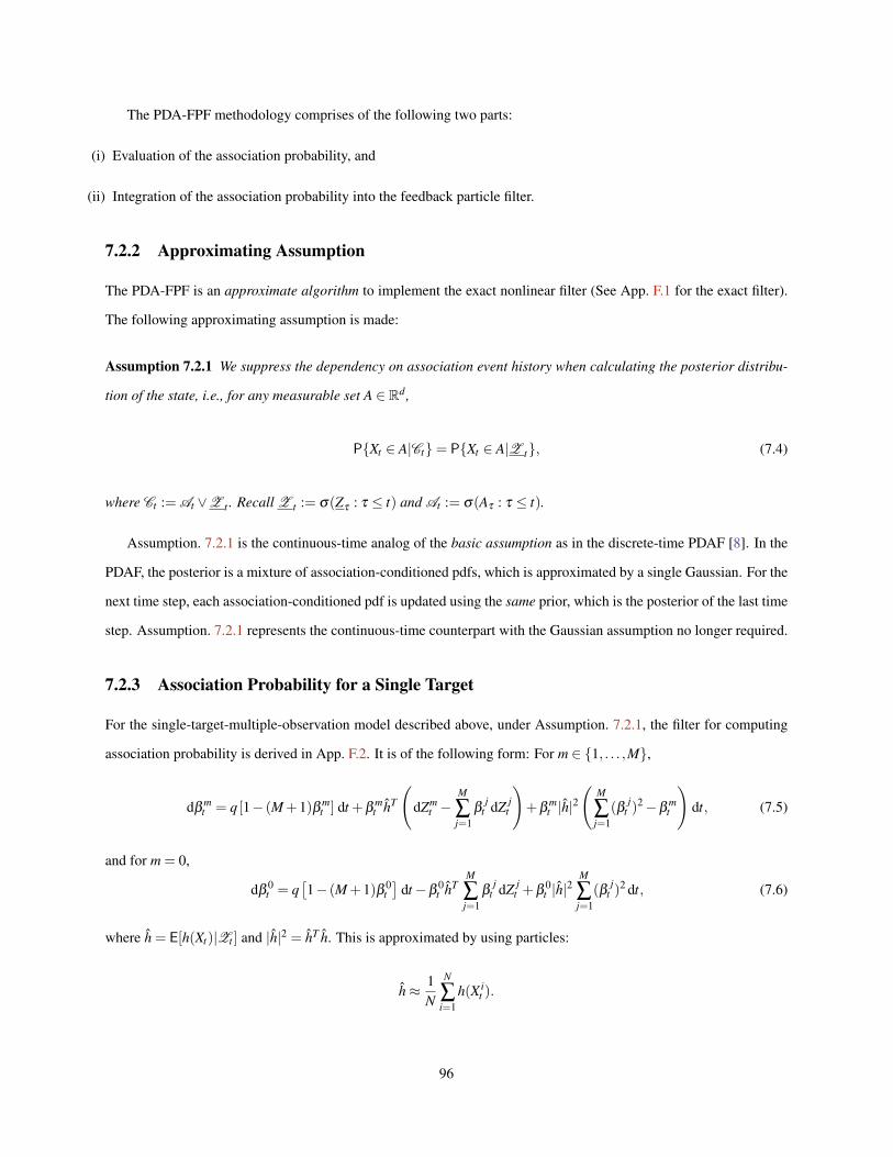
The PDA-FPF methodology comprises of the following two parts:
(i) Evaluation of the association probability, and
(ii) Integration of the association probability into the feedback particle filter.
7.2.2 Approximating Assumption
The PDA-FPF is an approximate algorithm to implement the exact nonlinear filter (See App. F.1 for the exact filter).
The following approximating assumption is made:
Assumption 7.2.1 We suppress the dependency on association event history when calculating the posterior distribu-
tion of the state, i.e., for any measurable set A ∈ Rd ,
PXt ∈ A|Ct= PXt ∈ A|Z t, (7.4)
where Ct := At ∨Z t . Recall Z t := σ(Zτ : τ ≤ t) and At := σ(Aτ : τ ≤ t).
Assumption. 7.2.1 is the continuous-time analog of the basic assumption as in the discrete-time PDAF [8]. In the
PDAF, the posterior is a mixture of association-conditioned pdfs, which is approximated by a single Gaussian. For the
next time step, each association-conditioned pdf is updated using the same prior, which is the posterior of the last time
step. Assumption. 7.2.1 represents the continuous-time counterpart with the Gaussian assumption no longer required.
7.2.3 Association Probability for a Single Target
For the single-target-multiple-observation model described above, under Assumption. 7.2.1, the filter for computing
association probability is derived in App. F.2. It is of the following form: For m ∈ 1, . . . ,M,
dβmt = q [1− (M+1)β m
t ] dt +βmt hT
(dZm
t −M
∑j=1
βj
t dZ jt
)+β
mt |h|2
(M
∑j=1
(β jt )
2−βmt
)dt, (7.5)
and for m = 0,
dβ0t = q
[1− (M+1)β 0
t]
dt−β0t hT
M
∑j=1
βj
t dZ jt +β
0t |h|2
M
∑j=1
(β jt )
2 dt, (7.6)
where h = E[h(Xt)|Zt ] and |h|2 = hT h. This is approximated by using particles:
h≈ 1N
N
∑i=1
h(X it ).
96

In practice, one may also wish to consider approaches to reduce filter complexity, e.g., by assigning gating regions for
the observations; cf., Sec. 4.2.3 in [9].
Remark 9 The association probability filter (7.5)-(7.6) can also be derived by considering a continuous-time limit
starting from the continuous-discrete time filter in literature [9]. This proof appears in App. F.3. The alternate proof
is included for the following reasons:
(i) The proof helps provide a comparison with the classical PDA filter. This is important because some of the
modeling assumptions (e.g., modeling of association At via a jump Markov process), at first sight, may appear to
be different from those considered in the classical literature.
(ii) The proof method suggests alternate discrete-time algorithms for evaluating association probability in simula-
tions and experiments, where observations are made at discrete sampling times.
In the following, we integrate association probability into the feedback particle filter, which is used to approximate
the evolution of the posterior distribution. The algorithmic structure – evaluation of data association probability
first, followed by its subsequent inclusion in the filter for approximating posterior – is motivated by the following
considerations:
(i) Such an algorithmic structure mirrors the structure used in the classical PDA filtering literature [8, 9, 97].
(ii) The computation of association probability depends upon the details of the clutter model – the present chapter
describes this computation for the Gaussian clutter case (see (7.5)-(7.6)). Once the association probability is com-
puted, the filtering equation for the state process does not depend upon the details of the clutter model. It is thus
presented separately, and can also be used as such.
(iii) A separate treatment is also useful while considering multiple target tracking problems. For such problems, one
can extend algorithms for data association in a straightforward manner, while the algorithm for posterior remains
as before. Additional details appear in Sec 7.3.
7.2.4 Probabilistic Data Association-Feedback Particle Filter
Following the feedback particle filter methodology, the model for the particle filter is given by,
dX it = a(X i
t )dt + dBit + dU i
t ,
where X it ∈ Rd is the state for the ith particle at time t, U i
t is its control input, and BitN
i=1 are mutually independent
standard Wiener processes. We assume the initial conditions X i0N
i=1 are i.i.d., independent of Bit, and drawn from
97
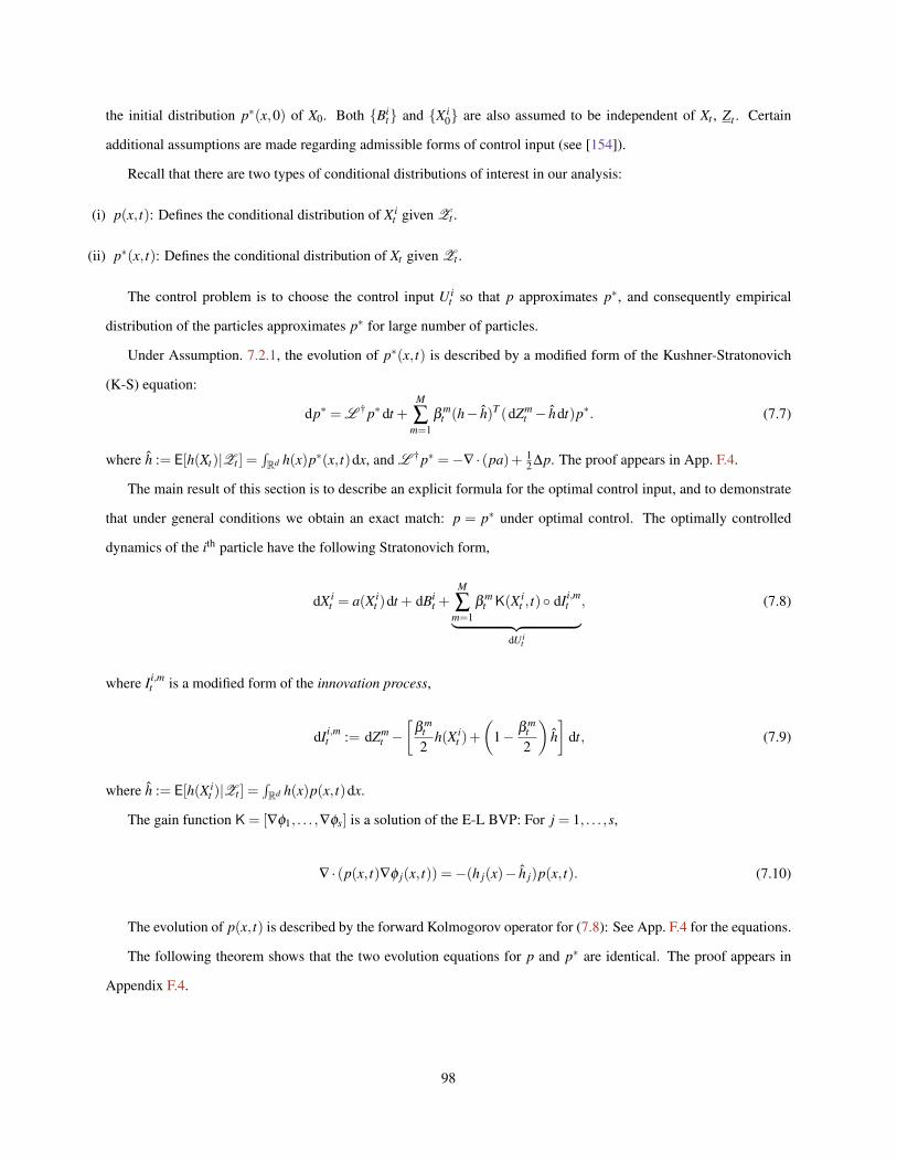
the initial distribution p∗(x,0) of X0. Both Bit and X i
0 are also assumed to be independent of Xt , Zt . Certain
additional assumptions are made regarding admissible forms of control input (see [154]).
Recall that there are two types of conditional distributions of interest in our analysis:
(i) p(x, t): Defines the conditional distribution of X it given Zt .
(ii) p∗(x, t): Defines the conditional distribution of Xt given Zt .
The control problem is to choose the control input U it so that p approximates p∗, and consequently empirical
distribution of the particles approximates p∗ for large number of particles.
Under Assumption. 7.2.1, the evolution of p∗(x, t) is described by a modified form of the Kushner-Stratonovich
(K-S) equation:
dp∗ = L † p∗ dt +M
∑m=1
βmt (h− h)T (dZm
t − hdt)p∗. (7.7)
where h := E[h(Xt)|Zt ] =∫Rd h(x)p∗(x, t)dx, and L † p∗ =−∇ · (pa)+ 1
2 ∆p. The proof appears in App. F.4.
The main result of this section is to describe an explicit formula for the optimal control input, and to demonstrate
that under general conditions we obtain an exact match: p = p∗ under optimal control. The optimally controlled
dynamics of the ith particle have the following Stratonovich form,
dX it = a(X i
t )dt + dBit +
M
∑m=1
βmt K(X i
t , t) dIi,mt︸ ︷︷ ︸
dU it
, (7.8)
where Ii,mt is a modified form of the innovation process,
dIi,mt := dZm
t −[
β mt
2h(X i
t )+
(1− β m
t
2
)h]
dt, (7.9)
where h := E[h(X it )|Zt ] =
∫Rd h(x)p(x, t)dx.
The gain function K = [∇φ1, . . . ,∇φs] is a solution of the E-L BVP: For j = 1, . . . ,s,
∇ · (p(x, t)∇φ j(x, t)) =−(h j(x)− h j)p(x, t). (7.10)
The evolution of p(x, t) is described by the forward Kolmogorov operator for (7.8): See App. F.4 for the equations.
The following theorem shows that the two evolution equations for p and p∗ are identical. The proof appears in
Appendix F.4.
98
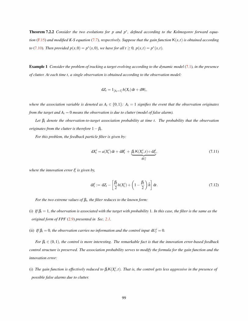
Theorem 7.2.2 Consider the two evolutions for p and p∗, defined according to the Kolmogorov forward equa-
tion (F.15) and modified K-S equation (7.7), respectively. Suppose that the gain function K(x, t) is obtained according
to (7.10). Then provided p(x,0) = p∗(x,0), we have for all t ≥ 0, p(x, t) = p∗(x, t).
Example 1 Consider the problem of tracking a target evolving according to the dynamic model (7.1), in the presence
of clutter. At each time t, a single observation is obtained according to the observation model:
dZt = 1[At=1] h(Xt)dt + dWt ,
where the association variable is denoted as At ∈ 0,1: At = 1 signifies the event that the observation originates
from the target and At = 0 means the observation is due to clutter (model of false alarm).
Let βt denote the observation-to-target association probability at time t. The probability that the observation
originates from the clutter is therefore 1−βt .
For this problem, the feedback particle filter is given by:
dX it = a(X i
t )dt + dBit + βt K(X i
t , t) dIit︸ ︷︷ ︸
dU it
, (7.11)
where the innovation error Iit is given by,
dIit := dZt −
[βt
2h(X i
t )+
(1− βt
2
)h]
dt. (7.12)
For the two extreme values of βt , the filter reduces to the known form:
(i) If βt = 1, the observation is associated with the target with probability 1. In this case, the filter is the same as the
original form of FPF (2.9) presented in Sec. 2.1.
(ii) If βt = 0, the observation carries no information and the control input dU it = 0.
For βt ∈ (0,1), the control is more interesting. The remarkable fact is that the innovation error-based feedback
control structure is preserved. The association probability serves to modify the formula for the gain function and the
innovation error:
(i) The gain function is effectively reduced to βtK(X it , t). That is, the control gets less aggressive in the presence of
possible false alarms due to clutter.
99
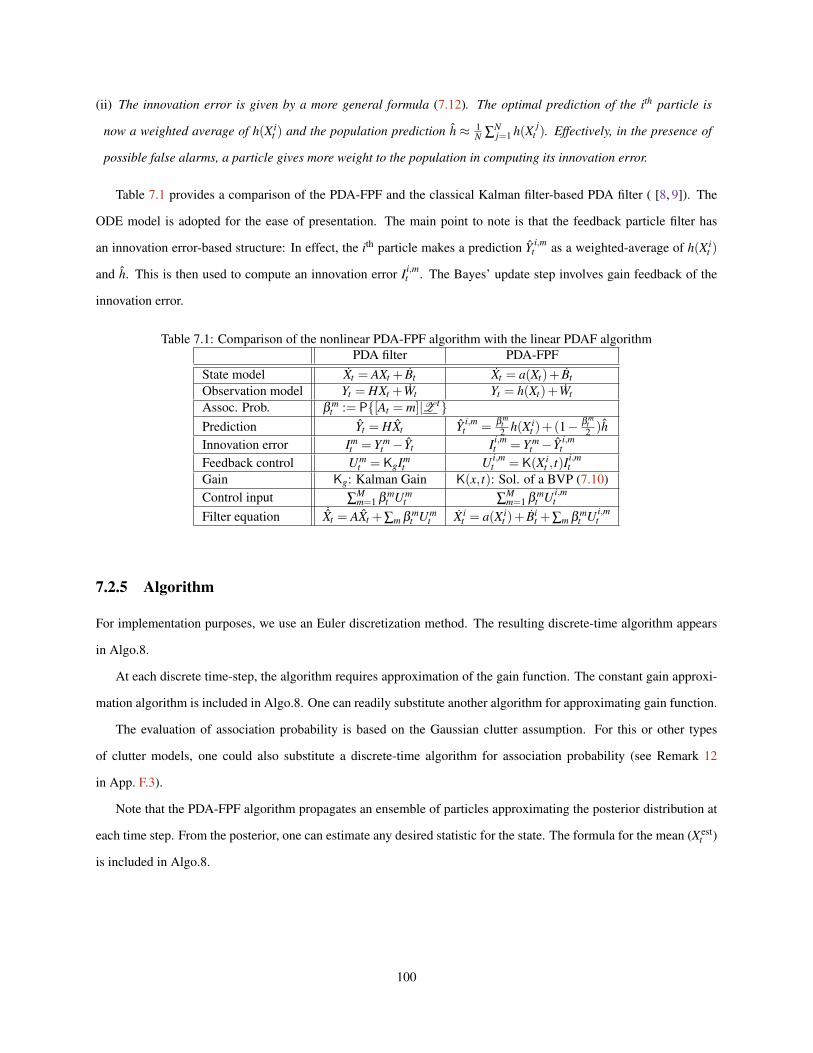
(ii) The innovation error is given by a more general formula (7.12). The optimal prediction of the ith particle is
now a weighted average of h(X it ) and the population prediction h ≈ 1
N ∑Nj=1 h(X j
t ). Effectively, in the presence of
possible false alarms, a particle gives more weight to the population in computing its innovation error.
Table 7.1 provides a comparison of the PDA-FPF and the classical Kalman filter-based PDA filter ( [8, 9]). The
ODE model is adopted for the ease of presentation. The main point to note is that the feedback particle filter has
an innovation error-based structure: In effect, the ith particle makes a prediction Y i,mt as a weighted-average of h(X i
t )
and h. This is then used to compute an innovation error Ii,mt . The Bayes’ update step involves gain feedback of the
innovation error.
Table 7.1: Comparison of the nonlinear PDA-FPF algorithm with the linear PDAF algorithmPDA filter PDA-FPF
State model Xt = AXt + Bt Xt = a(Xt)+ BtObservation model Yt = HXt +Wt Yt = h(Xt)+WtAssoc. Prob. β m
t := P[At = m]|Z tPrediction Yt = HXt Y i,m
t = β mt2 h(X i
t )+(1− β mt2 )h
Innovation error Imt = Y m
t − Yt Ii,mt = Y m
t − Y i,mt
Feedback control Umt = KgIm
t U i,mt = K(X i
t , t)Ii,mt
Gain Kg: Kalman Gain K(x, t): Sol. of a BVP (7.10)Control input ∑
Mm=1 β m
t Umt ∑
Mm=1 β m
t U i,mt
Filter equation ˙Xt = AXt +∑m β mt Um
t X it = a(X i
t )+ Bit +∑m β m
t U i,mt
7.2.5 Algorithm
For implementation purposes, we use an Euler discretization method. The resulting discrete-time algorithm appears
in Algo.8.
At each discrete time-step, the algorithm requires approximation of the gain function. The constant gain approxi-
mation algorithm is included in Algo.8. One can readily substitute another algorithm for approximating gain function.
The evaluation of association probability is based on the Gaussian clutter assumption. For this or other types
of clutter models, one could also substitute a discrete-time algorithm for association probability (see Remark 12
in App. F.3).
Note that the PDA-FPF algorithm propagates an ensemble of particles approximating the posterior distribution at
each time step. From the posterior, one can estimate any desired statistic for the state. The formula for the mean (Xestt )
is included in Algo.8.
100

Algorithm 8 PDA-FPF for tracking single target in clutter:1: INITIALIZATION2: for i = 1 to N do3: Sample X i
0 from p(x,0)4: end for5: for m = 0 to M do6: Set β m
0 = 1M+1 .
7: end for8: p(N)(x,0) = 1
N ∑Ni=1 δX i
0(x)
9: Xest0 = 1
N ∑Ni=1 X i
01: ITERATION [t to t +∆t]2: for i = 1 to N do3: Sample a Gaussian random vector ∆V4: Calculate h = 1
N ∑Ni=1 h(X i
t )
5: Calculate |h|2 = hT h6: Calculate the gain function K = 1
N ∑Ni=1 X i
t (h(Xit )− h)T
7: X it+∆t = X i
t +a(X it )∆t +∆V
√∆t
8: for m = 1 to M do9: Calculate ∆Ii,m
t = ∆Zmt −
[β m
t2 h(X i
t )+(1− β mt2 )h
]∆t
10: X it+∆t = X i
t+∆t +β mt K∆Ii,m
t
11: ∆β mt = q [1− (M+1)β m
t ]∆t +β mt hT
(∆Zm
t −∑Mj=1 β
jt ∆Z j
t
)+β m
t |h|2(
∑Mj=1(β
jt )
2−β mt
)∆t
12: β mt+∆t = β m
t +∆β mt .
13: end for14: end for15: t = t +∆t16: p(N)(x, t) = 1
N ∑Ni=1 δX i
t(x)
17: Xestt = 1
N ∑Ni=1 X i
t
101
7.2.6 Example: Linear Case
In this section, we illustrate the PDA-FPF with the aid of a linear example. The example also serves to provide a
comparison to the classic PDA filter. Consider the following linear model:
dXt = A Xt dt + dBt , (7.13a)
dZmt = 1[At=m] H Xt dt + dW m
t , (7.13b)
where A is a d×d matrix and H is an s×d matrix.
The PDA-FPF is described by (7.8)-(7.10). If we assume the initial distribution p∗(x,0) is Gaussian with mean
µ0 and covariance matrix Σ0, then the following lemma provides the solution of the gain function K(x, t) in the linear
case.
Lemma 7.2.3 Consider the linear observation (7.13b). Suppose p(x, t) is assumed to be Gaussian with mean µt and
variance Σt , i.e., p(x, t) = 1
(2π)d2 |Σt |
12
exp[− 1
2 (x−µt)T Σ−1t (x−µt)
]. Then the solution of the E-L BVP (7.10) is given
by:
K(x, t) = ΣtHT (7.14)
The formula (7.14) is verified by direct substitution in (7.10) where the distribution p is Gaussian.
The linear PDA-FPF is then given by,
dX it = A X i
t dt + dBit +ΣtHT
M
∑m=1
βmt
(dZm
t −H[
β mt
2X i
t +
(1− β m
t
2
)µt
]dt). (7.15)
Note that there is no Wong-Zakai correction term since the gain function is constant.
The following theorem states that p = p∗ in this case. That is, the conditional distributions of Xt and X it coincide.
The proof is a straightforward extension of the proof in App. F.4, and is thus omitted.
Theorem 7.2.4 Consider the single target tracking problem with a linear model defined by the state-observation
equations (7.13a,7.13b). The PDA-FPF is given by (7.15). In this case the posterior distributions of Xt and X it
coincide, whose conditional mean and covariance are given by the following,
dµt = Aµt dt +ΣtHTM
∑m=1
βmt (dZm
t −Hµt dt) , (7.16)
dΣt
dt= AΣt +ΣtAT + I−
M
∑m=1
(β mt )2
ΣtHT HΣt . (7.17)
102

(7.16)-(7.17) is consistent with the linear PDAF result [9]. In other words, the PDA-FPF reduces to the classic PDAF
in the linear case.
The filter for association probability β mt in the linear Gaussian case easily follows from using (7.5). It is of the
following form: for m = 1, . . . ,M,
dβmt = q [1− (M+1)β m
t ] dt +βmt (Hµt)
T
(dZm
t −M
∑j=1
βj
t dZ jt
)+β
mt (Hµt)
T (Hµt)
(M
∑j=1
(β jt )
2−βmt
)dt. (7.18)
In practice µt ,Σt in (7.15)-(7.18) are approximated as sample means and sample covariances from the ensemble
X it N
i=1.
µt ≈ µ(N)t :=
1N
N
∑i=1
X it ,
Σt ≈ Σ(N)t :=
1N−1
N
∑i=1
(X i
t −µ(N)t
)(X i
t −µ(N)t
)T.
7.3 Multiple Target Tracking using the Feedback Particle Filter
In this section, we extend the PDA-FPF to the multiple target tracking (MTT) problem. The resulting filter is referred
to as the joint probabilistic data association-feedback particle filter (JPDA-FPF). For notational ease, we assume a
clutter free scenario where all observations originate from the targets (i.e., there are M targets and M observations at
each time). The clutter can be handled in a manner similar to the basic PDA-FPF.
The MTT problem is introduced in Sec. 7.3.1. The algorithm is described only for the special case of two targets
with two observations (M = 2), in Sec. 7.3.2. The algorithm for the general case is conceptually analogous but
notationally cumbersome. It appears in Appendix. F.5.
7.3.1 Problem Statement, Assumptions and Notation
The following notation is adopted:
(i) There are M distinct targets. The set of targets is denoted by the index set M = 1,2, . . . ,M. The set of permu-
tations of M is denoted by Π(M ), whose cardinality |Π(M )| = M!. A typical element of Π(M ) is denoted as
α = (α1,α2, . . . ,αM).
(ii) At time t, the state of the nth target is denoted as Xnt ∈ Rd for n ∈M .
(iii) At time t, there is exactly one observation per target for a total of M observations, all of which are available in a
centralized fashion. The observation vector is denoted by Zt := (Z1t ,Z
2t , . . . ,Z
Mt ), where the mth entry, Zm
t ∈ Rs,
originates from one of the targets in M .
103
(iv) At time t, the association random vector is denoted as At ∈ Π(M ). It is used to associate targets with the observa-
tions in a joint manner: At := (α1t ,α
2t , . . . ,α
Mt ) ∈Π(M ) signifies that the observation Z1
t originates from target α1t ,
Z2t originates from target α2
t , . . . , ZMt originates from target αM
t .
The following models are assumed for the three stochastic processes.
(i) The dynamics of the nth target evolves according to the nonlinear SDE:
dXnt = an(Xn
t )dt + dBnt , (7.19)
where Bnt ∈ Rd are mutually independent standard Wiener processes and n ∈M .
(ii) The observation model is given by:
dZ1
t...
dZMt
= Ψ(At)
h(X1
t )
...
h(XMt )
dt +
dW 1
t...
dW Mt
, (7.20)
where Ψ(At) is the permutation matrix for association vector At , and W mt M
m=1 are mutually independent standard
Wiener processes, also assumed to be mutually independent with Bnt .
(iii) The model for At is similar to the model assumed in PDA-FPF (see Sec. 7.2) and is described by a continuous-time
Markov chain:
P[At+∆t = γ]|[At = γ′]= q∆t +o(∆t), γ 6= γ
′ ∈Π(M ), (7.21)
where, for the ease of presentation, the transition rate is assumed to be a constant q. The initial distribution is
assumed given.
(iv) At and X t are assumed to be mutually independent.
The problem is to design M feedback particle filters, where the nth filter is intended to estimate the posterior
distribution of the nth target given the history of all un-associated observations (filtration) Zt := σ (Zτ : τ ≤ t).
The joint association probability is defined as the probability of the joint association event [At = γ] conditioned on
Zt :
πγ
t := P[At = γ]|Zt, γ ∈Π(M ). (7.22)
The filter for the joint association probability πγ
t is a notationally tedious but straightforward extension of the
association filter in PDA-FPF (7.5). It appears in App. F.5.
104

The joint association probabilities are then used to obtain association probability for each individual target. Once
the observation-to-target association probability is known, its integration into the feedback particle filter is identical to
the PDA-FPF (7.8). The complete set of equations for the JPDA-FPF algorithm appear in App. F.5. The M = 2 case
is illustrated next.
7.3.2 Example: Two-Target Two-Observation Problem
At time t, the target state is denoted as X t := (X1t ,X
2t ), and the observation vector Zt := (Z1
t ,Z2t ). The association
random vector is denoted as At ∈ Π(1,2) := γ1,γ
2, where γ
1:= (1,2) and γ
2:= (2,1). It is used to associate
observations to targets: At = γ1
signifies that Z1t originates from target 1 and Z2
t from target 2; At = γ2
accounts for
the complementary case.
The following models are assumed for the three stochastic processes:
(i) Each element of the state vector X t evolves according to a nonlinear SDE of the form (7.1):
dXnt = an(Xn
t )dt + dBnt , n ∈ 1,2, (7.23)
where B1t ,B2
t are mutually independent standard Wiener processes.
(ii) The association random process At evolves as a jump Markov process in continuous-time:
P[At+∆t = γm′ ]|[At = γ
m]= q∆t +o(∆t), m′ 6= m ∈ 1,2.
The initial distribution is assumed given.
(iii) At and X t are assumed to be mutually independent.
(iv) At time t, the observation model is given by,
dZ1t
dZ2t
= Ψ(At)
h(X1t )
h(X2t )
dt +
dW 1t
dW 2t
,where W 1
t ,W 2t are mutually independent Wiener processes and Ψ(At) is a function mapping At to a permutation
matrix:
Ψ(γ1) =
Is 0
0 Is
, Ψ(γ2) =
0 Is
Is 0
,where Is is the s× s identity matrix.
105
The joint association probability is defined as the probability of the joint association [At = γ] conditioned on Zt :
πmt := P[At = γ
m]|Zt, m ∈ 1,2.
Based on the JPDA-FPF algorithm discussed in App. F.5, the filter for joint association probability π1t is (under
Assumption. 7.2.1):
dπ1t =−q(π1
t −π2t )dt +π
1t π
2t
ˆhT (dZ1t − dZ2
t )− (π1t −π
2t )π
1t π
2t
∣∣∣ ˆh∣∣∣2 dt,
where h(X1t ,X
2t ) := h(X1
t )−h(X2t ),
ˆh :=E[h|Zt ] and∣∣∣ ˆh∣∣∣2 = ˆhT ˆh. The expectations are approximated by using particles.
Since the joint events are mutually exclusive and exhaustive, we have ∑2m=1 πm
t = 1. Using this, we have π2t = 1−π1
t
and dπ2t =−dπ1
t .
The joint association probabilities π1t ,π
2t are used to obtain association probability for individual target. For
example, for target 1: β1,1t = π1
t , β2,1t = π2
t , where βm,nt denotes the conditional probability that the mth observation
originates from the nth target. Once the association probability is known, the feedback particle filter for each target is
of the form (7.8). The detailed algorithm for JPDA-FPF is omitted because of its similarity to PDA-FPF.
7.4 Numerics
7.4.1 Single Target Tracking in Clutter
Consider first the problem of tracking a single target in clutter. The target evolves according to a white-noise acceler-
ation model:
dXt = FXt dt +σB dBt , (7.24)
dZt = HXt dt +σW dWt , (7.25)
where Xt denotes the state vector comprising of position and velocity coordinates at time t, Zt is the observation
process, Bt,Wt are mutually independent standard Wiener processes. The two matrices are given by:
F =
0 1
0 0
, H =
[1 0
].
In the simulation results described next, the following parameter values are used: σB = (0,1), σW = 0.06, and
106
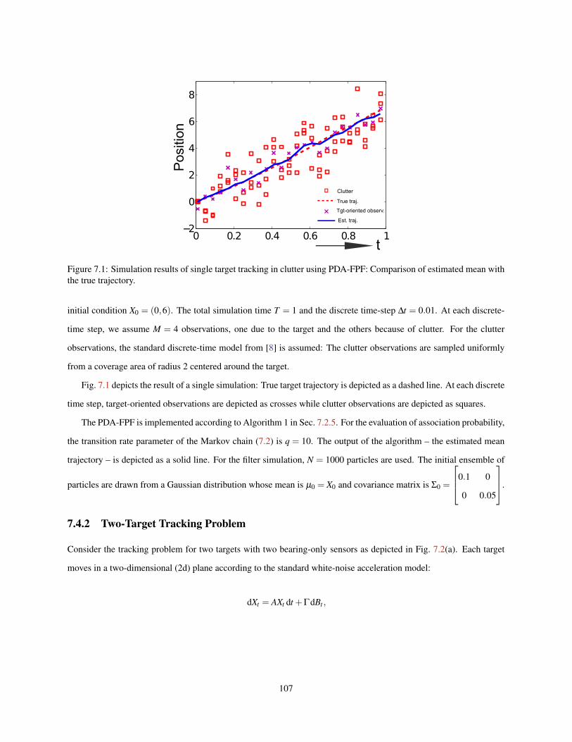
0 0.2 0.4 0.6 0.8 1−2
0
2
4
6
8
t
Pos
ition
Clutter
True traj.
Tgt-oriented observ.
Est. traj.
Figure 7.1: Simulation results of single target tracking in clutter using PDA-FPF: Comparison of estimated mean withthe true trajectory.
initial condition X0 = (0,6). The total simulation time T = 1 and the discrete time-step ∆t = 0.01. At each discrete-
time step, we assume M = 4 observations, one due to the target and the others because of clutter. For the clutter
observations, the standard discrete-time model from [8] is assumed: The clutter observations are sampled uniformly
from a coverage area of radius 2 centered around the target.
Fig. 7.1 depicts the result of a single simulation: True target trajectory is depicted as a dashed line. At each discrete
time step, target-oriented observations are depicted as crosses while clutter observations are depicted as squares.
The PDA-FPF is implemented according to Algorithm 1 in Sec. 7.2.5. For the evaluation of association probability,
the transition rate parameter of the Markov chain (7.2) is q = 10. The output of the algorithm – the estimated mean
trajectory – is depicted as a solid line. For the filter simulation, N = 1000 particles are used. The initial ensemble of
particles are drawn from a Gaussian distribution whose mean is µ0 = X0 and covariance matrix is Σ0 =
0.1 0
0 0.05
.
7.4.2 Two-Target Tracking Problem
Consider the tracking problem for two targets with two bearing-only sensors as depicted in Fig. 7.2(a). Each target
moves in a two-dimensional (2d) plane according to the standard white-noise acceleration model:
dXt = AXt dt +ΓdBt ,
107
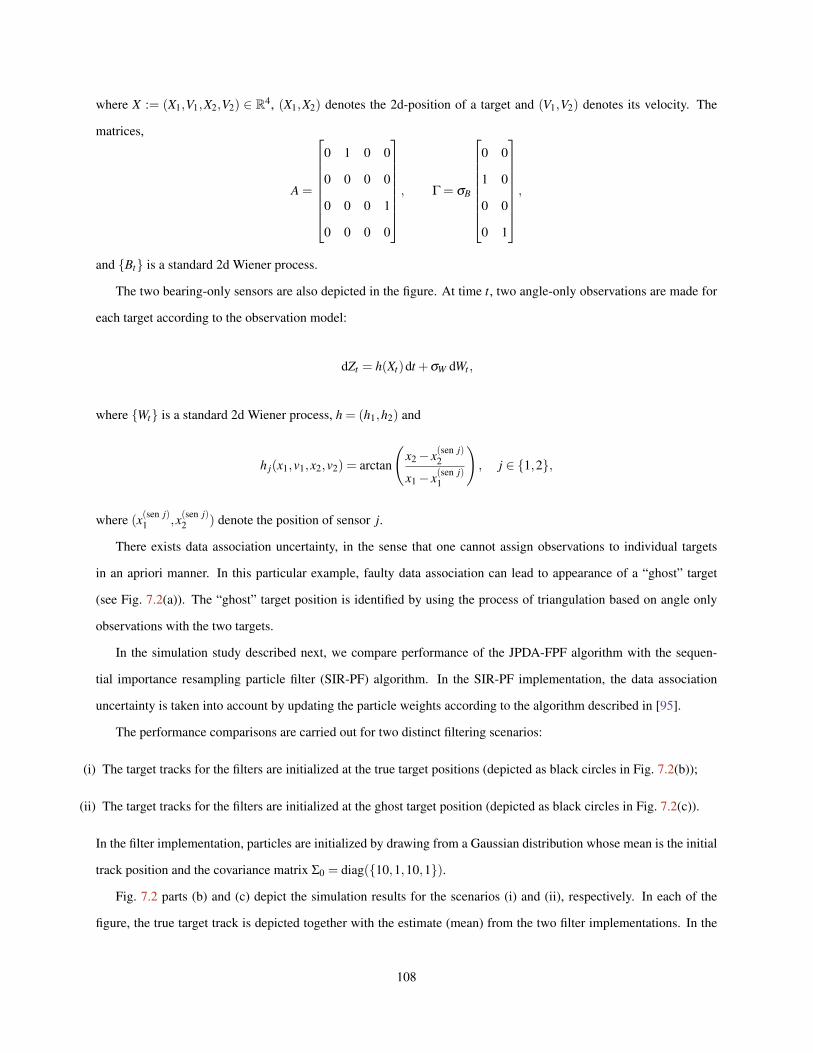
where X := (X1,V1,X2,V2) ∈ R4, (X1,X2) denotes the 2d-position of a target and (V1,V2) denotes its velocity. The
matrices,
A =
0 1 0 0
0 0 0 0
0 0 0 1
0 0 0 0
, Γ = σB
0 0
1 0
0 0
0 1
,
and Bt is a standard 2d Wiener process.
The two bearing-only sensors are also depicted in the figure. At time t, two angle-only observations are made for
each target according to the observation model:
dZt = h(Xt)dt +σW dWt ,
where Wt is a standard 2d Wiener process, h = (h1,h2) and
h j(x1,v1,x2,v2) = arctan
(x2− x(sen j)
2
x1− x(sen j)1
), j ∈ 1,2,
where (x(sen j)1 ,x(sen j)
2 ) denote the position of sensor j.
There exists data association uncertainty, in the sense that one cannot assign observations to individual targets
in an apriori manner. In this particular example, faulty data association can lead to appearance of a “ghost” target
(see Fig. 7.2(a)). The “ghost” target position is identified by using the process of triangulation based on angle only
observations with the two targets.
In the simulation study described next, we compare performance of the JPDA-FPF algorithm with the sequen-
tial importance resampling particle filter (SIR-PF) algorithm. In the SIR-PF implementation, the data association
uncertainty is taken into account by updating the particle weights according to the algorithm described in [95].
The performance comparisons are carried out for two distinct filtering scenarios:
(i) The target tracks for the filters are initialized at the true target positions (depicted as black circles in Fig. 7.2(b));
(ii) The target tracks for the filters are initialized at the ghost target position (depicted as black circles in Fig. 7.2(c)).
In the filter implementation, particles are initialized by drawing from a Gaussian distribution whose mean is the initial
track position and the covariance matrix Σ0 = diag(10,1,10,1).
Fig. 7.2 parts (b) and (c) depict the simulation results for the scenarios (i) and (ii), respectively. In each of the
figure, the true target track is depicted together with the estimate (mean) from the two filter implementations. In the
108
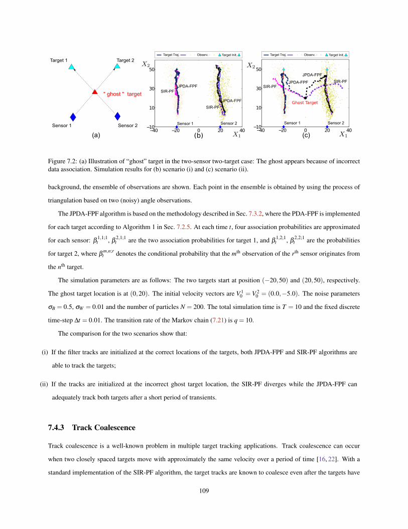
−40 −20 0 20 40−10
10
30
50
Sensor 1 Sensor 2
SIR-PFJPDA-FPF
JPDA-FPF
SIR-PF
−40 −20 0 20 40−10
10
30
50
SIR-PF
Sensor 1 Sensor 2
JPDA-FPF
SIR-PFJPDA-FPF
Ghost Target
(b)(a) (c)
Target Traj. Target Init.Observ. Target Traj. Target Init.Observ.
Figure 7.2: (a) Illustration of “ghost” target in the two-sensor two-target case: The ghost appears because of incorrectdata association. Simulation results for (b) scenario (i) and (c) scenario (ii).
background, the ensemble of observations are shown. Each point in the ensemble is obtained by using the process of
triangulation based on two (noisy) angle observations.
The JPDA-FPF algorithm is based on the methodology described in Sec. 7.3.2, where the PDA-FPF is implemented
for each target according to Algorithm 1 in Sec. 7.2.5. At each time t, four association probabilities are approximated
for each sensor: β1,1;1t , β
2,1;1t are the two association probabilities for target 1, and β
1,2;1t , β
2,2;1t are the probabilities
for target 2, where βm,n;rt denotes the conditional probability that the mth observation of the rth sensor originates from
the nth target.
The simulation parameters are as follows: The two targets start at position (−20,50) and (20,50), respectively.
The ghost target location is at (0,20). The initial velocity vectors are V 10 = V 2
0 = (0.0,−5.0). The noise parameters
σB = 0.5, σW = 0.01 and the number of particles N = 200. The total simulation time is T = 10 and the fixed discrete
time-step ∆t = 0.01. The transition rate of the Markov chain (7.21) is q = 10.
The comparison for the two scenarios show that:
(i) If the filter tracks are initialized at the correct locations of the targets, both JPDA-FPF and SIR-PF algorithms are
able to track the targets;
(ii) If the tracks are initialized at the incorrect ghost target location, the SIR-PF diverges while the JPDA-FPF can
adequately track both targets after a short period of transients.
7.4.3 Track Coalescence
Track coalescence is a well-known problem in multiple target tracking applications. Track coalescence can occur
when two closely spaced targets move with approximately the same velocity over a period of time [16, 22]. With a
standard implementation of the SIR-PF algorithm, the target tracks are known to coalesce even after the targets have
109
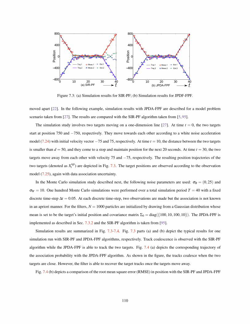
0 10 20 30 40−800
−400
0
400
800
Pos
ition
(a) SIR-PF0 10 20 30 40
−800
−400
0
400
800
Pos
ition
(b) JPDA-FPF
Traj.1
Traj.2
Meas.1
Meas.2
Est.1
Est.2
Traj.1
Traj.2
Meas.1
Meas.2
Est.1
Est.2
Figure 7.3: (a) Simulation results for SIR-PF; (b) Simulation results for JPDF-FPF.
moved apart [22]. In the following example, simulation results with JPDA-FPF are described for a model problem
scenario taken from [27]. The results are compared with the SIR-PF algorithm taken from [5, 95].
The simulation study involves two targets moving on a one-dimension line [27]. At time t = 0, the two targets
start at position 750 and −750, respectively. They move towards each other according to a white noise acceleration
model (7.24) with initial velocity vector−75 and 75, respectively. At time t = 10, the distance between the two targets
is smaller than d = 50, and they come to a stop and maintain position for the next 20 seconds. At time t = 30, the two
targets move away from each other with velocity 75 and −75, respectively. The resulting position trajectories of the
two targets (denoted as X tgtt ) are depicted in Fig. 7.3. The target positions are observed according to the observation
model (7.25), again with data association uncertainty.
In the Monte Carlo simulation study described next, the following noise parameters are used: σB = (0,25) and
σW = 10. One hundred Monte Carlo simulations were performed over a total simulation period T = 40 with a fixed
discrete time-step ∆t = 0.05. At each discrete time-step, two observations are made but the association is not known
in an apriori manner. For the filters, N = 1000 particles are initialized by drawing from a Gaussian distribution whose
mean is set to be the target’s initial position and covariance matrix Σ0 = diag(100,10,100,10). The JPDA-FPF is
implemented as described in Sec. 7.3.2 and the SIR-PF algorithm is taken from [95].
Simulation results are summarized in Fig. 7.3-7.4. Fig. 7.3 parts (a) and (b) depict the typical results for one
simulation run with SIR-PF and JPDA-FPF algorithms, respectively. Track coalescence is observed with the SIR-PF
algorithm while the JPDA-FPF is able to track the two targets. Fig. 7.4 (a) depicts the corresponding trajectory of
the association probability with the JPDA-FPF algorithm. As shown in the figure, the tracks coalesce when the two
targets are close. However, the filter is able to recover the target tracks once the targets move away.
Fig. 7.4 (b) depicts a comparison of the root mean square error (RMSE) in position with the SIR-PF and JPDA-FPF
110

0 10 20 30 400
0.2
0.4
0.6
0.8
1
Pro
babi
lity
(a) Assoc. Probability
SIR PF
JPDA-FPF
Pos
ition
RM
SE
(b) Comparison0 10 20 30 400
50
100
150
200
Figure 7.4: (a) Plot of data association probability; (b) Comparison of RMSE with SIR-PF and JPDA-FPF
algorithms. The RMSE at time t is defined as:
RMSEt =
√E
[∣∣∣Xestt −X tgt
t
∣∣∣2],where E[·] is computed by taking the average of 100 Monte Carlo runs. For t < 30, the performance of the two
algorithms is comparable. However once the two closely spaced targets depart away from each other, the RMSE of
SIR-PF soars while the JPDA-FPF remains relatively stable.
Table 7.2: Comparison between SIR PF and JPDA-FPFMethod Avg. RMSE Avg. % Tracks “OK”SIR-PF 75.40 78JPDA-FPF 22.86 100
Table 7.2 provides a summary of the performance with the two algorithms. The metrics are average RMSE and
the average percentage of the filter tracks being “OK.” The average RMSE is calculated as:
avg. RMSE =
√1T
∫ T
0E
[∣∣∣Xestt −X tgt
t
∣∣∣2] dt.
A track is said to be “OK” if the average tracking error satisfies:
√1T
∫ T
0
∣∣∣Xestt −X tgt
t
∣∣∣2 dt ≤ 9σW .
The metrics used here are borrowed from [29, 95].
111

7.5 Conclusion
In this chapter, we introduced a novel feedback control-based particle filter algorithm for the filtering problem with
data association uncertainty. The algorithm is referred to as the probabilistic data association-feedback particle filter
(PDA-FPF). PDA-FPF provides for a generalization of the Kalman filter-based PDA filter to a general class of non-
linear non-Gaussian problems. Our proposed algorithm inherits many of the properties that has made the Kalman
filter-based algorithms so widely applicable over the past five decades, including innovation error and the feedback
structure (see Fig. 2.1).
The feedback structure is important on account of the issue of robustness. The structural aspects are also expected
to be useful for design, integration and testing of the algorithm in a larger system involving filtering problems (e.g.,
navigation systems).
Several numerical examples were included to illustrate the theoretical results, and provide comparisons with the
SIR particle filter. Notably, simulation results suggest that track coalescence, which is a well-known problem in MTT
applications, can be avoided by the proposed JPDA-FPF algorithm. A complete numerical comparison, in terms of
tracking performance with the existing approaches, for MTT applications is planned for future publications.
112

Part III
Appendices
113

Appendix A
Proofs for Chapter 2
A.1 Calculation of K-L divergence
Recall the definition of K-L divergence for densities,
D(pn‖p∗n) =∫R
pn(s) ln( pn(s)
p∗n(s)
)ds.
We make a co-ordinate transformation s = x+ v(x) and use (2.15) to express the K-L divergence as:
D(pn‖p∗n) =∫R
p−n (x)|1+ v′(x)| ln(
p−n (x)|1+ v′(x)| p∗n(x+ v(x))
)|1+ v′(x)|dx
The expression for K-L divergence given in (2.17) follows on using (2.14).
A.2 Solution of the Optimization Problem
Denote:
L (x,v,v′) =−p−n (x)(
ln |1+ v′|+ ln(p−n (x+ v)pY |X(Ytn |x+ v))). (A.1)
The optimization problem (2.16) is a calculus of variation problem:
minv
∫L (x,v,v′)dx.
The minimizer is obtained via the analysis of first variation given by the well-known Euler-Lagrange equation:
∂L
∂v=
ddx
(∂L
∂v′
),
Explicitly substituting the expression (A.1) for L , we obtain (2.18).
114

A.3 Derivation of the Forward Equation
We denote the filtration Bt = σ(X i0,B
is : s≤ t), and we recall that Zt = σ(Zs : s≤ t) for t ≥ 0. These two filterations
are independent by construction.
On denoting a(x, t) = a(x)+u(x, t), the particle evolution (2.19) is expressed,
X it = X i
0 +∫ t
0a(X i
s ,s)ds+∫ t
0K(X i
s ,s)dZ(s)+σBBit . (A.2)
By assumption on Lipschitz continuity of a and K, there exists a unique solution that is adapted to the larger filtration
Bt ∨Zt = σ(X i0,B
is,Zs : s≤ t). In fact, there is a functional Ft such that,
X it = Ft(X i
0,Bit ,Z
t), (A.3)
where Zt := Zs : 0≤ s≤ t denotes the trajectory.
The conditional distribution of X it given Zt = σ(Zs : s ≤ t) was introduced in Sec. 2.2.1: Its density is denoted
p(x, t), defined by any bounded and measurable function f : R→ R via,
E[ f (X it ) |Zt ] =
∫R
p(x, t) f (x)dx =: 〈pt , f 〉.
We begin with a result that is the key to proving Prop. 2.3.1. The proof of the Lemma A.3.1 below appears in [156].
It is omitted here on account of space.
Lemma A.3.1 Suppose that f is an Bt ∨Zt -adapted process satisfying E∫ t
0 | f (s)|2 ds< ∞. Then,
E[∫ t
0f (s)ds|Zt
]=∫ t
0E[ f (s)|Zs]ds, (A.4)
E[∫ t
0f (s)dZs|Zt
]=∫ t
0E[ f (s)|Zs]dZs. (A.5)
ut
We now provide a proof of the Prop. 2.3.1.
Proof of Proposition 2.3.1 Applying Ito’s formula to equation (2.19) gives, for any smooth and bounded function
f ,
d f (X it ) = L f (X i
t )dt +σB∂ f∂x
(X it )dBi
t +K(X it , t)
∂ f∂x
(X it )dZt ,
115
where L f := (a+u) ∂ f∂x +
12 (σ
2W K2 +σ2
B)∂ 2 f∂x2 . Therefore,
f (X it ) = f (X i
0)+∫ t
0L f (X i
s)ds+σB
∫ t
0
∂ f∂x
(X is)dBi
s +∫ t
0K(X i
s ,s)∂ f∂x
(X is)dZs.
Taking conditional expectations on both sides,
〈pt , f 〉= E[ f (X i0) |Zt ]+E
[∫ t
0L f (X i
s)ds|Zt
]+σBE
[∫ t
0
∂ f∂x
(X is)dBi
s |Zt
]+E[∫ t
0K(X i
s ,s)∂ f∂x
(X is)dZs |Zt
]
On applying Lemma A.3.1, and the fact that Bit is a Wiener process, we conclude that
〈pt , f 〉= 〈p0, f 〉+∫ t
0〈ps,L f 〉ds+
∫ t
0〈ps,K
∂ f∂x〉dZs .
The forward equation (2.22) follows using integration by parts.
A.4 Euler-Lagrange Equation for the Continuous-Time Filter
In this section we describe, formally, the continuous-time limit of the discrete-time E-L BVP (2.18). In the continuous-
time case, the control and the observation models are of the form (see (2.19) and (2.1b)):
dU it = u(X i
t , t)dt +K(X it , t)dZt ,
dZt = h(Xt)dt +σW dWt .
In discrete-time, these are approximated as
4U it = u(X i
t , t)4t +K(X it , t)4Zt , (A.6)
4Zt = h(Xt)4t +σW4Wt ,
where 4t is the small time-increment at t. It follows that the conditional distribution of Yt.= 4Zt4t given Xt is the
density,
pY |X(Yt |·) =1√
2πσ2W/4t
exp(− (4Zt −h(·)4t)2
2σ2W4t
). (A.7)
Substituting (A.6)-(A.7) in the E-L BVP (2.18) for the continuous-discrete time case, we arrive at the formal
116
equation:
∂
∂x
(p(x, t)
1+u′4t +K′4Zt
)= p(x, t)
∂
∂v
(ln p(x+ v, t)+ ln pY |X(Yt | x+ v)
)∣∣∣∣v=u4t+K4Zt
. (A.8)
For notational ease, we use primes to denote partial derivatives with respect to x: p is used to denote p(x, t),
p′ := ∂ p∂x (x, t), p′′ := ∂ 2 p
∂x2 (x, t), u′ := ∂u∂x (x, t), K′ := ∂K
∂x (x, t) etc. Note that the time t is fixed.
A sketch of calculations to obtain (2.23) and (2.24) starting from (A.8) appears in the following three steps:
Step 1: The three terms in (A.8) are simplified as:
∂
∂x
(p
1+u′4t +K′4Zt
)= p′− f14t− (p′K′+ pK′′)4Zt
p∂
∂vln p(x+ v)
∣∣∣∣v=u4t+K4Zt
= p′+ f24t +(p′′K− p′2K
p)4Zt
p∂
∂vln pY |X(Yt |x+ v)
∣∣∣∣v=u4t+K4Zt
=p
σ2W(h′4Zt −hh′4t)+ ph′′K4t
where we have used Ito’s rules (4Zt)2 = σ2
W4t, 4Zt4t = 0 etc., and where
f1 = (p′u′+ pu′′)−σ2W (p′K′2 +2pK′K′′),
f2 = (p′′u− p′2up
)+σ2W K2
(12
p′′′− 3p′p′′
2p+
p′3
p2
).
Collecting terms in O(4Zt) and O(4t), after some simplification, leads to the following ODEs:
E (K) =1
σ2W
h′(x) (A.9)
E (u) =− 1σ2
Wh(x)h′(x)+h′′(x)K+σ
2W G(x, t) (A.10)
where E (K) =− ∂
∂x
(1
p(x,t)∂
∂xp(x, t)K(x, t)), and G =−2K′K′′− (K′)2(ln p)′+ 1
2 K2(ln p)′′′.
Step 2. Suppose (u,K) are admissible solutions of the E-L BVP (A.9)-(A.10). Then it is claimed that
−(pK)′ =h− hσ2
Wp (A.11)
−(pu)′ =− (h− h)hσ2
Wp− 1
2σ
2W (pK2)′′. (A.12)
Recall that admissible here means
limx→±∞
p(x, t)u(x, t) = 0, limx→±∞
p(x, t)K(x, t) = 0. (A.13)
117
To show (A.11), integrate (A.9) once to obtain
−(pK)′ =1
σ2W
hp+Cp,
where the constant of integration C = − hσ2
Wis obtained by integrating once again between −∞ to ∞ and using the
boundary conditions for K (A.13). This gives (A.11).
To show (A.12), we denote its right hand side as R and claim
(R
p
)′=− hh′
σ2W
+h′′K+σ2W G. (A.14)
The equation (A.12) then follows by using the ODE (A.10) together with the boundary conditions for u (A.13). The
verification of the claim involves a straightforward calculation, where we use (A.9) to obtain expressions for h′ and
K′′. The details of this calculation are omitted on account of space.
Step 3. On integrating (A.9), we obtain the E-L equation for K, which is the same as (2.23). The proof of (2.24)
involves a short calculation starting from (A.12), which is simplified to the form (2.24) by using (A.11).
Remark 10 The derivation of Euler-Lagrange equation, as presented above, is a heuristic on account of Step 1. A
similar heuristic also appears in the original paper of Kushner [100]. There, the Kushner-Stratonovich PDE (2.21)
is derived by considering a continuous-time limit of the Bayes formula (2.14). The Ito’s rules are used to obtain the
limit. Rigorous justification of the calculation in Step 1, or its replacement by an alternate argument is the subject of
future work.
The calculation in Steps 2 and 3 require additional regularity assumptions on density p and function h: p is C3
and h is C2.
A.5 Proof of Prop. 2.3.2.
Consider the ODE (2.23). It is a linear ODE whose unique solution is given by
K(x, t) =1
p(x, t)
(C1 +C2
∫ x
−∞
p(y, t)dy− 1σ2
W
∫ x
−∞
h(y)p(y, t)dy), (A.15)
where the constant of integrations C1 = 0 and C2 =ht
σ2W
because of the boundary conditions for K. Part 2 is an easy
consequence of the minimum principle for elliptic PDEs [60].
118

A.6 Proof of Thm. 2.3.3
It is only necessary to show that with this choice of u,K, we have dp(x, t) = dp∗(x, t), for all x and t, in the
sense that they are defined by identical stochastic differential equations. Recall dp∗ is defined according to the K-S
equation (2.21), and dp according to the forward equation (2.22).
If K solves the E-L BVP (2.23) then using (A.15),
∂
∂x(pK) =− 1
σ2W(h− h)p. (A.16)
On multiplying both sides of (2.24) by −p, we have
−up =12(h− h)pK− 1
2σ
2W (pK)
∂ K
∂x+ hpK
=−12
σ2W
∂ (pK)
∂xK− 1
2σ
2W (pK)
∂ K
∂x+ hpK
=−12
σ2W
∂
∂x(pK2)+ hpK,
where we have used (A.16) to obtain the second equality. Differentiating once with respect to x and using (A.16) once
again,
− ∂
∂x(up)+
12
σ2W
∂ 2
∂x2 (pK2) =− hσ2
W(h− h)p. (A.17)
Using (A.16)-(A.17) in the forward equation (2.22), we have
dp = L † p+1
σ2W(h− h)(dZt − hdt)p .
This is precisely the SDE (2.21), as desired.
A.7 Proof of Thm. 2.3.5
The Gaussian density is given by:
p(x, t) =1√
2πΣtexp(− (x−µt)
2
2Σt
), (A.18)
The density (A.18) is a function of the stochastic process µt . Using Ito’s formula,
dp(x, t) =∂ p∂ µ
dµt +∂ p∂Σ
dΣt +12
∂ 2 p∂ µ2 dµ
2t ,
where ∂ p∂ µ
= x−µtΣt
p, ∂ p∂Σ
= 12Σt
((x−µt )
2
Σt−1)
p, and ∂ 2 p∂ µ2 = 1
Σt
((x−µt )
2
Σt−1)
p. Substituting these into the forward equa-
119
tion (2.22), we obtain a quadratic equation Ax2 +Bx = 0, where
A = dΣt −(
2αΣt +σ2B−
γ2Σ2t
σ2W
)dt,
B = dµt −(
αµt dt +γΣt
σ2W(dZt − γµt dt)
).
This leads to the model (2.28) and (2.29). ut
120
Appendix B
Proofs for Chapter 3
B.1 Proof of Thm. 3.2.2
It is only necessary to show that with the choice of u,K given by (3.13)-(3.14), we have dp(x, t) = dp∗(x, t), for all
x and t, in the sense that they are defined by identical stochastic differential equations. Recall dp∗ is defined according
to the K-S equation (3.10), and dp according to the forward equation (3.12).
Recall that the gain function K is a solution of the following BVP:
∇ · (pK) =−p(h− h)T . (B.1)
On multiplying both sides of (3.14) by −p, we obtain
−up =12
p(h− h)K−Ωp+ pKh
=−12
K[∇ · (pK)]T −Ωp+ pKh(B.2)
where (B.1) is used to obtain the second equality. Denoting E := 12 K[∇ · (pK)]T , a direct calculation shows that
El +Ωl p =d
∑k=1
∂
∂xk
(p[KKT ]lk
).
Substituting this in (B.2), on taking the divergence of both sides, we obtain
−∇ · (pu)+12
d
∑l,k=1
∂ 2
∂xl∂xk
(p[KKT ]lk
)= ∇ · (pK) h. (B.3)
Using (B.1) and (B.3) in the forward equation (3.12),
dp = L † p+(h− h)T (dZt − hdt)p.
This is precisely the SDE (3.10), as desired. ut
121

B.2 BVP for the Multivariable Feedback Particle Filter
Consider the multivariable linear system,
dXt = αXt dt +σB dBt (B.4a)
dZt = γT Xt dt +σW dWt (B.4b)
where Xt ∈ Rd , Zt ∈ R1, α is an d× d matrix, γ is an d× 1 vector, Bt is an d−dimensional Wiener process, Wt
is a scalar Wiener process, and Bt,Wt are assumed to be mutually independent. We assume the initial distribution
p∗(x,0) is Gaussian with mean vector µ0 and variance matrix Σ0.
The following proposition shows that the Kalman gain is a solution of the multivariable BVP (3.17), the Kalman
gain solution does not equal the solution Kg (see (3.20)), and that the solution given by Kg is not integrable with
respect to p:
Proposition B.2.1 Consider the d-dimensional linear system (B.4a)-(B.4b), where d ≥ 2. Suppose p(x, t) is assumed
to be Gaussian: p(x, t) = 1
(2π)d2 |Σt |
12
exp(− 1
2 (x−µt)T Σ−1t (x−µt)
), where x = (x1,x2, ...,xd)
T , µt is the mean, Σt is
the covariance matrix, and |Σt |> 0 denotes the determinant.
1) One solution of the BVP (3.17) is given by the Kalman gain:
K(x, t) =1
σ2W
Σtγ (B.5)
2) Suppose that the Kalman gain K given in (B.5) is non-zero. For this solution to (3.17), there does not exist a
function φ such that pK = ∇φ .
3) Consider the solution Kg(x, t) of the BVP (3.17) as given by (3.20). This gain function is unbounded: |Kg(x, t)| →
∞ as |x| → ∞, and moreover
∫Rd|Kg(x, t)|p(x, t)dx = ∞,
∫Rd|Kg(x, t)|2 p(x, t)dx = ∞.
ut
Proof The Kalman gain solution (B.5) is verified by direct substitution in the BVP (3.17) where the distribution
p is Gaussian.
The proof of claim 2 follows by contradiction. Suppose a function φ exists such that pK = ∇φ , then we have
∂ (Kp)i
∂x j=
∂ 2φ
∂x j∂xi=
∂ 2φ
∂xi∂x j=
∂ (Kp) j
∂xi, ∀i, j (B.6)
122
where (Kp)i is the ith entry of vector Kp. By direct evaluation, we have
∂ (Kp)i
∂x j= 2Ki ·
(Σ−1t (x−µt)
)j p.
Using (B.6), we obtain
Ki(Σ−1t ) jk = K j(Σ
−1t )ik, ∀i, j,k (B.7)
Setting k = i, summing over the index i and using (B.5), we arrive at
tr(Σ−1t )K = Σ
−1t K,
where tr(Σ−1t ) denotes the trace of the matrix Σ
−1t . This provides a contradiction because K 6≡ 0 and Σt is a positive
definite symmetric matrix with |Σt |> 0.
We now establish claim 3. For the solution Kg as given by (3.20):
pKg(x, t) =1
σ2W
1dωd
∫ y− x|y− x|d (h(y)− h)p(y, t)dy
For this integral, with h(y)≡ γT y, we have the following asymptotic formula for |x| ∼ ∞,
pKg(x, t)∼C1|x|d +o
(1|x|d),
where C does not vary as a function of |x| (its value depends only upon the angular coordinates). For example, in
dimension d = 2, C is given by
C(x1,x2) =C(|x|cos(θ), |x|sin(θ))
=− 1dωd
cos(2θ) sin(2θ)
sin(2θ) cos(2θ)
Σtγ
σ2W,
where Σt γ
σ2W
is the Kalman gain vector.
The result follows because 1p|x|d → ∞ and 1
|x|d is not integrable in Rd . Using the Cauchy-Schwarz inequality,
∫|Kg(x, t)|p(x, t)dx≤
(∫|Kg(x, t)|2 p(x, t)dx
) 12,
which shows that Kg is not square-integrable.
123

B.3 Proof of Thm. 3.3.1
We omit the subscript “ j” in this proof, writing just φ and h. We also suppress explicit dependence on time t, writing
p(x) instead of p(x, t) and φ(x) instead of φ(x, t).
Under Assumption A1, p is known to admit a spectral gap (or Poincare inequality) with constant λ ≥ c1 [87]: That
is, for all functions φ ∈ H10 (Rd ; p),
∫|φ(x)|2 p(x)dx≤ 1
λ
∫|∇φ(x)|2 p(x)dx. (B.8)
Consider now the inner product
< φ ,ψ >:=∫
∇φ(x) ·∇ψ(x)p(x)dx.
On account of (B.8), the norm defined by using the inner product < ·, · > is equivalent to the standard norm in
H1(Rd ; p).
(i) Consider the BVP in its weak form (3.25). The integral on the righthand-side is a bounded linear functional on
ψ ∈ H10 , since
∣∣∣∣∫ (h(x)− h)ψ(x)p(x)dx∣∣∣∣2 ≤ ∫ |h(x)− h|2 p(x)dx
∫|ψ(x)|2 p(x)dx
≤ (const.)∫|∇ψ(x)|2 p(x)dx,
where (B.8) is used to obtain the second inequality.
It follows from the Reisz representation theorem that there exists a unique φ ∈ H10 such that
< φ ,ψ >=∫(h(x)− h)ψ(x)p(x)dx,
for all ψ ∈ H10 (Rd ; p). Thus φ is a weak solution of the BVP, satisfying (3.25).
(ii) Suppose φ is a weak solution. Using ψ = φ in (3.25),
∫|∇φ |2 p(x)dx =
∫(h(x)− h)φ(x)p(x)dx≤
(∫|h(x)− h|2 p(x)dx
) 12(∫|φ(x)|2 p(x)dx
) 12
≤(∫|h(x)− h|2 p(x)dx
) 12(
1λ
∫|∇φ(x)|2 p(x)dx
) 12
by (B.8). The estimate (3.27) follows.
124

(iii) For the final estimate (3.28), we need:
Lemma B.3.1 Under Assumptions A1-A4, the weak solution φ of the BVP (3.25) belongs to H2(Rd ; p), with
∫|D2
φ |2 pdx≤∫
∇φ ·Gpdx (B.9)
where the vector function G ∈ L2(Rd ; p) is defined by
G = D2(log p)∇φ +∇h
and where |D2φ |2 = ∑ j,k(∂ 2φ
∂x j∂xk)2.
Proof First note that each entry of the Hessian matrix D2(log p) is bounded, by Assumption A3, and that ∇h ∈
L2(Rd ; p) by Assumption A4. Hence G ∈ L2(R; p).
Next, elliptic regularity theory [60, Section 6.3 of the PDE text by Evans] applied to the weak solution φ ∈H1(Rd ; p)
says that φ ∈ H3loc(R
d). Hence the partial differential equation holds pointwise:
−∇ · (p∇φ) = (h− h)p. (B.10)
We differentiate with respect to xk to obtain:
−∇ ·(
p∇∂φ
∂xk
)−∇
(∂ log p
∂xk
)· (p∇φ)− ∂ log p
∂xk∇ · (p∇φ) =
∂h∂xk
p+(h− h)∂ log p
∂xkp.
The final terms on the left and right sides cancel, by equation (B.10). Thus the preceding formula becomes
−∇ ·(
p∇∂φ
∂xk
)= Gk p, (B.11)
where Gk denotes the kth component of G(x).
Let β (x)≥ 0 be a smooth, compactly supported “bump” function, meaning β (x) is radially decreasing with β (0) =
1. Let s> 0 and multiply (B.11) by β (sx)2 ∂φ
∂xk. Integrate by parts on the left side (noting the boundary terms vanish
because β has compact support) to obtain
∫∇
[β (sx)2 ∂φ
∂xk
]· (∇ ∂φ
∂xk)pdx =
∫β (sx)2 ∂φ
∂xkGk pdx.
125

The right hand side RHS→ ∫ ∂φ
∂xkGk pdx by dominated convergence as s→ 0, since β (0) = 1. The left side,
LHS =∫
β (sx)2∣∣∣∣∇ ∂φ
∂xk
∣∣∣∣2 pdx+2s∫
∂φ
∂xkβ (sx)(∇β )(sx) ·
(∇
∂φ
∂xk
)pdx.
Clearly the second term is bounded by
2s‖∇β‖L∞(Rd)
∫ ∣∣∣∣ ∂φ
∂xk
∣∣∣∣β (sx)∣∣∣∣∇ ∂φ
∂xk
∣∣∣∣ pdx≤ s‖∇β‖L∞(Rd)
∫ [(∂φ
∂xk
)2
+β (sx)2∣∣∣∣∇ ∂φ
∂xk
∣∣∣∣2]
pdx
and so
(1− s‖∇β‖L∞(Rd)
)∫β (sx)2
∣∣∣∣∇ ∂φ
∂xk
∣∣∣∣2 pdx− s‖∇β‖L∞(Rd)
∫ (∂φ
∂xk
)2
dx≤ LHS.
Letting s→ 0 in LHS and RHS, and recalling that β (x) is radially decreasing, we conclude from the monotone
convergence theorem that ∫ ∣∣∣∣∇ ∂φ
∂xk
∣∣∣∣2 pdx≤∫
∂φ
∂xkGk pdx.
Summing over k completes the proof of the lemma.
Next we prove (3.28). We will use several times that
∫|∇φ |2 pdx≤ 1
λ
∫|h− h|2 pdx≤ 1
λ 2
∫|∇h|2 pdx, (B.12)
by (3.27) followed by (B.8) applied to the function h− h ∈ H10 (Rd ; p).
We have
∫ ∣∣(D2φ)(∇φ)
∣∣ pdx≤∫|D2
φ ||∇φ |pdx≤(
1λ 2
∫|∇h|2 pdx
)3/4(∫|G|2 pdx
)1/4
by Lemma B.3.1, Cauchy–Schwarz, and (B.12). The definition of G, the L2-triangle inequality and (B.12) show
that
(∫|G|2 pdx
)1/2
≤ ‖D2(log p)‖L∞
(∫|∇φ |2 pdx
)1/2
+
(∫|∇h|2 pdx
)1/2
≤(‖D2(log p)‖L∞
λ+1)(∫
|∇h|2 pdx)1/2
.
The estimate (3.28) now follows.
126
Appendix C
Proofs for Chapter 4
C.1 Proof of Prop. 4.2.2
Differentiating ρ∗n (x,λ ) in (4.8) with respect to λ , and subsequent evaluation yields:
∂ρ∗(x,λ )∂λ
=1∫
exp fn(x′,λ )dx′∂ exp fn(x,λ )
∂λ− exp fn(x,λ )
[∫
exp fn(x′,λ )dx′]2∂∫
exp fn(x′,λ )dx′
∂λ
=exp fn(x,λ )∫
exp fn(x′,λ )dx′∂ fn(x,λ )
∂λ− exp fn(x,λ )
[∫
exp fn(x′,λ )dx′]2
∫exp fn(x′,λ )
∂ fn(x′,λ )∂λ
dx′
= ρ∗n (x,λ )
[∂ fn(x,λ )
∂λ−∫
ρ∗n (x′,λ )
∂ fn(x′,λ )∂λ
dx′]
= ρ∗n (x,λ ) ·
[h(x)T [Yn−
12
h(x)]−∫
ρ∗n (x′,λ )h(x′)T [Yn−
12
h(x′)]dx′]
= ρ∗n (x,λ ) ·
[(h(x)− hn(λ ))
TYn−12|h(x)|2 + 1
2
∫ρ∗n (x′,λ )|h(x′)|2 dx′
], (C.1)
where we define hn(λ ) :=∫
ρ∗n (x,λ )h(x)dx and |h(·)|2 := h(·)T h(·). Equation (C.1) is exactly (4.9) as desired. ut
C.2 Proof of Thm. 4.2.3
It is only necessary to show that with this choice of u,K ((4.12)-(4.14)), we have that dρ(x,λ ) = dρ∗(x,λ ), for all
x and λ ∈ [0,1], in the sense that they are defined by identical SDEs. Recall that dρ∗ is described as in (4.9), and dρ
according to the forward equation (4.11).
If φ j solves the E-L BVP (4.12) then using K = [∇φ T1 , . . . ,∇φ T
m ] we have,
∇ · (ρK) =−(h(x)− h)Tρ. (C.2)
127
On multiplying both sides of (4.13) by −ρ and then taking the gradient, we obtain
−∇ · (ρu) =12
∇ · (ρK(h+ h))− 12
∇ · (ρΩ)
=−12(h− h)T (h− h)+
12
ρ
m
∑j=1
∇φ j ·∇hTj −
12
∇ · (ρΩ)
=−12|h|2 + 1
2|h|2, (C.3)
where we use (C.2) and (4.14) to get the second and third equality, respectively.
Using (C.2)-(C.3) in the forward equation (4.11), we have
dρ = ρ
[(h(x)− h)TYn−
12
(|h|2− |h|2
)].
This is precisely the SDE (4.9), as desired. ut
C.3 Proof of Prop. 4.2.4
Formula (4.19) is verified by direct substitution in the BVP (4.12) where the distribution ρ is multivariate Gaussian.
To verify (4.20), first by taking the gradient of (4.19) we obtain:
∇φ j =[[Σλ HT ]1 j, . . . , [Σλ HT ]d j
]. (C.4)
Substituting (C.4) to (4.14),
∇ · (ρΩ) =12
[µ
Tλ
HT Hµλ − XT HT HX +m
∑j=1
d
∑k=1
H jk[Σλ HT ]k j
]. (C.5)
Recall that:
Σλ = XXT −µλ µTλ,
and consider the gradient-form solution Ω = ∇ϕ , we have the RHS of (C.5):
∇ · (ρ∇ϕ) = 0.
This leads to the unique solution Ω = (0, . . . ,0) which is (4.20).
128

Appendix D
Proofs for Chapter 5
D.1 Derivation of the Forward Equation
We denote the filtration Bt = σ(X i0,N
ll′,is , Nk,i
s : s≤ t), where Nk,is denote the Poisson counters with constant rate λ = 1,
for k = 1,2, . . . ,d. We recall that Zt = σ(Zs : s≤ t) for t ≥ 0. These two filtrations are independent by construction.
The particle evolution (5.5) is expressed,
X it = X i
0 + ∑(l,l′)∈E
∫ t
0All′X i
s dNll′,is +
d
∑k=1
∫ t
0BkX i
s dC k,is .
For the linear system, there exists a unique solution that is adapted to the larger filtration Bt∨Zt =σ(X i0,N
ll′,is , Nk,i
s ,Zs :
s≤ t). In fact, there is a functional Ft such that,
X it = Ft(X i
0,Nll′,i[0:t], N
k,i[0:t],Z[0:t]), (D.1)
where Z[0:t] := Zs : 0≤ s≤ t denotes the trajectory.
The conditional distribution of X it given Zt = σ(Zs : s≤ t) was introduced in Sec. 5.2: Its density is denoted p(·, t),
defined by any bounded function φ : S→ R via,
E[φ(X it ) |Zt ] =
d
∑l=1
p(l, t)φ l =: 〈pt ,φ〉,
where φ l := φ(el) and with slight abuse of notation we write φ = (φ 1,φ 2, . . . ,φ l).
We begin with a result that is the key to proving Prop. 5.2.1.
129
Lemma D.1.1 Suppose that f is an Bt ∨Zt -adapted process satisfying E∫ t
0 | f (s)|2 ds< ∞. Then,
E[∫ t
0f (s)ds|Zt
]=∫ t
0E[ f (s)|Zs]ds, (D.2)
E[∫ t
0f (s)dNl,l′,i
s |Zt
]=∫ t
0E[ f (s)|Zs]λl′l ds. (D.3)
E[∫ t
0f (s)dC k,i
s |Zt
]=∫ t
0E[ f (s)|Zs](K(k,s)dZs +u(k,s)ds). (D.4)
We now provide a proof of the Proposition 5.2.1.
Proof of Proposition 5.2.1 Applying Ito’s Lemma to equation (5.5) gives, for any bounded function φ : S→ R,
dφ(X it ) = L φ(X i
t )dt +d
∑k=1
[φ(X i
t +BkX it )−φ(X i
t )]
dC k,it ,
where L φ(el) := ∑dl′=1 λl′lφ(el′). Therefore,
φ(X it ) = φ(X i
0)+∫ t
0L φ(X i
s)ds+d
∑k=1
∫ t
0
[φ(X i
s +BkX is)−φ(X i
s)]
dC k,is .
Taking conditional expectation on both sides,
〈pt ,φ〉= E[φ(X i0)|Z ]+E
[∫ t
0L φ(X i
s)ds|Z]+
d
∑k=1
E
[∫ t
0[φ(X i
s +BkX is)−φ(X i
s)]dC k,is |Z
].
Using Lemma D.1.1, we have that
〈pt ,φ〉= 〈p0,φ〉+∫ t
0〈ps,L φ〉ds+
d
∑k=1
∫ t
0〈ps,φ(X i
s +BkX is)−φ(X i
s)〉(K(k,s)dZs +u(k,s)ds).
Using integration by parts and the definition of Bk we conclude that:
dp(k, t) =d
∑l=1
λkl p(l, t)dt + ∑k′ 6=k
(K(k, t)dZt +u(k, t)dt)p(k′, t)− ∑l′ 6=k
(K(l′, t)dZt +u(l′, t)dt)p(k, t), k = 1, . . . ,d.
(D.5)
The forward equation (5.8) follows by expressing equation (D.5) in the vector form. ut
We now provide a proof of Lemma D.1.1.
Proof of Lemma D.1.1 The key is the functional form (D.1) of the solution X it : It says that apart from the past values
of Zt , the solution depends only upon initial condition X i0 and time homogeneous Poisson process Nk,i
t and Nll′,it that
are all independent of Zt .
130

First we suppose that f , K and u are simple, i.e.,
f (s) =m
∑j=1
Fj1(a j ,b j ](s),
K(k,s) =m
∑j=1
Kkj1(a j ,b j ](s), u(k,s) =
m
∑j=1
ukj1(a j ,b j ](s).
where (a j,b j] are disjoint intervals of [0, t]. For general f , K and u satisfying the assumptions of the lemma, the result
will then follow via an application of the dominated convergence theorem.
Once we restrict to simple functions, the essence of the proof is to establish the identity,
E(Fj|Zt) = E(Fj|Za j). (D.6)
Under the measurability assumption we can write Fj = Ψ(ζ ,ξ ), where ζ ∈Za j , ξ ∈Ba j are random variables, and
Ψ is a real-valued function. The random variable ξ is independent of Zt , so that
E(Fj|Zt) = E(Ψ(ζ )|Zt),
with Ψ( ·) = E[Ψ( · ,ξ )]. Using the fact that ζ ∈Za j ⊂Zt we obtain (D.6):
E(Fj|Zt) = E(Ψ(ζ )|Zt) = E(Fj|Za j).
The desired results follow easily from (D.6): To obtain (D.2),
E(∫ t
0f (s)ds |Zt) =
m
∑j=1
E(Fj(b j−a j) |Zt) =m
∑j=1
E(Fj |Za j)(b j−a j)
=∫ t
0E( f (s) |Zs)ds,
To obtain (D.3):
E[∫ t
0f (s)dNll′,i
s |Zt
]=
m
∑j=1
E[Fj(Nll′,ib j−Nll′,i
a j) |Zt ] =
m
∑j=1
E[Fj |Za j ]E[Nll′,ib j−Nll′,i
a j]
=m
∑j=1
E[Fj |Za j ]λl′l(b j−a j)
=∫ t
0E[ f (s) |Zs]λl′l ds,
where the third equality uses the facts Nll′,it is a homogeneous Poisson process with rate λl′l . The proof of (D.4) is
131
similar:
E[∫ t
0f (s)dC k,i
s |Zt
]=
m
∑j=1
E[Fj(Ck,ib j−C k,i
a j) |Zt ] =
m
∑j=1
E[Fj |Za j ]E[Ck,ib j−C k,i
a j|Zt ]
=m
∑j=1
E[Fj |Za j ][Kkj(Zb j −Za j)+uk
j(b j−a j)]
=∫ t
0E[ f (s) |Zs](K(k,s)dZs +u(k,s)ds).
where the third equality follows from the following facts that: (i) C k,it is a non-homogeneous Poisson process with
E[C k,it −C k,i
s |Zt ] =∫ t
s K(k,τ)dZτ +u(k,τ)dτ; (ii) Zt is adapted to Zt , and ai < bi ≤ t for each i. ut
D.2 Proof of Prop. 5.2.2.
The matrix, D := (pt ⊗ 1− I), has rank d− 1 with null-space N (D) = spanpt and N (DT ) = span1. By the
application of the closed-range theorem:
(i) A solution exists because the righthand-side, −Ht pt , lies in the complement of N (DT ):
〈1,−Ht pt〉=−d
∑l=1
(h(l)− ht)p(l, t) = 0.
(ii) A unique solution exists in the complement of N (D). Denote it as K0t . By construction 〈K0
t , pt〉 = 0 and it is the
minimal 2-norm solution.
That Ht pt is a particular solution is verified by direct substitution. The form of the general solution (5.11) then
follows. The explicit formula for K0t is obtained by choosing c such that 〈K0
t , pt〉= 〈Ht pt + cpt , pt〉= 0.
The property (P0) is verified by direct substitution. For p(k, t) = 0, the kth equation of (5.9) is given by,
−K(k, t) = 0.
132
Appendix E
Proofs for Chapter 6
E.1 Derivation of the Exact Filtering Equations (6.6)-(6.9)
Derivation of (6.6): For each fixed mode θt = em ∈ e1,e2, . . . ,eM, the state process Xt is a Markov process with
Kolmogorov forward operator L †m . Therefore, the joint process (Xt ,θt)
T is a Markov process with generator L † +Q
where L † := diagL †m. Defining
∫A π∗m(x, t)dx := PXt ∈ A,θt = em and π∗(x, t) := (π∗1 (x, t), · · · ,π∗M(x, t))T we
have that∂π∗
∂ t(x, t) = L †
π∗(x, t)+QT
π∗(x, t).
Recall that the posterior distribution was defined by∫
A q∗m(x, t)dx := P[Xt ∈ A,θt = em]|Z . By applying the
fundamental filtering theorem for Gaussian observations (see [107]) to (6.3) we have:
dq∗m =L †m(q
∗m)dt +
M
∑l=1
qlmq∗l dt +(hm− ht)(dZt − ht dt)q∗m,
where ht := ∑Mm=1
∫R hm(x)q∗m(x, t)dx. ut
Derivation of (6.7) and (6.8): By definition, we have,
p∗(x, t) =M
∑m=1
q∗m(x, t), (E.1)
µmt =
∫R
q∗m(x, t)dx. (E.2)
Taking derivatives on both sides of (E.1) and (E.2) gives the desired result. ut
Derivation of (6.9): By definition q∗m = ρ∗mµmt . Applying Ito’s differentiation rule we have:
dρ∗m =
dq∗mµm
t+q∗m d
(1
µmt
)+ dq∗m d
(1
µmt
), (E.3)
where d(
1µm
t
)=− dµm
t(µm
t )2 +(dµm
t )2
(µmt )3 . Substituting (6.6) and (6.7) into (E.3) we obtain the desired result. ut
133
E.2 Proof of Consistency for IMM-FPF
We express the feedback particle filter (6.11) as:
dX i;mt = am(X i;m
t )dt +σm dBi;m
t +Km(X i;mt , t)dZt + u(X i;m
t , t)dt +um(X i;mt ,X i;−m
t )dt,
where
u(x, t) =−12
Km(x, t)(hm(x)+ hmt )+Ω(x, t), (E.4)
and Ω := 12 Km(Km)′ is the Wong-Zakai correction term for (6.11). The evolution equation for ρm is given by:
dρm =L †mρm dt− ∂
∂x(ρmKm)dZt −
∂
∂x(ρmu)dt− ∂
∂x(ρmum)dt +
12
∂ 2
∂x2
(ρm(K
m)2) dt. (E.5)
The derivation of this equation is similar to the basic FPF case (see Proposition 2 in [156]) and thus omitted here.
It is only necessary to show that with the choice of Km,um according to (6.13)-(6.14), we have dρm(x, t) =
dρ∗m(x, t), for all x and t, in the sense that they are defined by identical stochastic differential equations. Recall dρ∗m is
defined according to the modified K-S equation (6.9), and dρm according to the forward equation (E.5).
If Km solves the E-L BVP (6.13) then we have:
∂
∂x(ρmKm) =−(hm− hm
t )ρm. (E.6)
On multiplying both sides of (E.4) by −ρm, we have:
−ρmu =12(hm− hm
t )ρmKm− 12(ρmKm)
∂ Km
∂x+ hm
t ρmKm
=−12
∂ (ρmKm)
∂xKm− 1
2(ρmKm)
∂ Km
∂x+ hm
t ρmKm
=−12
∂
∂x
(ρm(K
m)2)+ hmt ρmKm
where we used (E.6) to obtain the second equality. Differentiating once with respect to x and using (E.6) once again,
− ∂
∂x(ρmu)+
12
∂ 2
∂x2
(ρm(K
m)2)=−hmt (h
m− hmt )ρm. (E.7)
Substituting (6.13), (6.14) and (E.7) to (E.5) and after some simplifications, we obtain:
dpm = L †m pm dt +(hm− hm
t )(dZt − hmt dt)pm +
1µm
t
M
∑l=1
qlmµlt (ρl−ρm)dt.
134

This is precisely the SDE (6.9), as desired.
E.3 Alternate Derivation of (6.15)
The aim of this section is to derive, formally, the update part of the continuous time filter (6.15) by taking a continuous
time limit of the discrete-time algorithm for evaluation of association probability. The procedure for taking the limit
is similar to Sec 6.8 in [86] for derivation of the K-S equation.
At time t, we have M possible modes for the SHS. The discrete-time filter for mode association probability is
obtained by using Bayes’ rule (see [10]):
Pθt = em|Z ,∆Zt=P∆Zt |θt = emPθt = em|Z
∑Ml=1 P∆Zt |θt = elPθt = el |Z
. (E.8)
Rewrite:
P∆Zt |θt = em=∫
P∆Zt |θt = em,Xt = xρm(x, t)dx
= Lm(∆Zt). (E.9)
where Lm(∆Zt) := 1√2π∆t
∫R exp
[− (∆Zt−hm(x)∆t)2
2∆t
]ρm(x, t)dx.
Now, recall µmt = Pθt = em|Z , the increment in the measurement update step (see Sec 6.8 in [86]) is given by
∆µmt := Pθt = em|Z ,∆Zt−Pθt = em|Z . (E.10)
Using (E.8) and (E.10), we have:
∆µmt = Em(∆t,∆Zt)µ
mt −µ
mt , (E.11)
where
Em(∆t,∆Zt) =Pθt = em|Z ,∆Zt
Pθt = em|Z . (E.12)
We expand Em(∆t,∆Zt) as a multivariate series about (0,0):
Em(∆t,∆Zt) = Em(0,0)+Em∆t(0,0)∆t +Em
∆Zt(0,0)∆Zt +
12
Em∆Zt ,∆Zt
(0,0)dZ2t +o(∆t). (E.13)
135
By direct evaluation, we obtain:
Em(0,0) = 1,
Em∆t(0,0) =
12
(h2
t − (hmt )
2), Em
∆Zt(0,0) = hm
t − ht
Em∆Zt ,∆Zt
(0,0) = (hmt )
2−2hmt ht +2h2
t − h2t
where (hmt )
2 :=∫R(h
m(x))2ρm(x, t)dx and h2t := ∑
Mm=1 µm
t (hmt )
2.
By using Ito’s rules,
E[∆Zt∆Zt ] = ∆t.
This gives
Em(∆t,∆Zt) = 1+(hmt − ht)(∆Zt − ht∆t) (E.14)
Substituting (E.14) to (F.11) we obtain the expression for ∆µmt , which equals the measurement update part of the
continuous-time filter.
Remark 11 During a discrete-time implementation, one can use (E.8)-(F.7) to obtain association probability. In (E.8),
Lm(dZt) is approximated by using particles:
Lm(∆Zt)≈1N
1√2π∆t
N
∑i=1
exp
[− (∆Zt −hm(X i;m
t )∆t)2
2∆t
].
136

Appendix F
Proofs for Chapter 7
F.1 Exact Filter for p∗
The exact nonlinear filter for p∗ is derived as an application of IMM-FPF, which is described in Sec. 6.2.
Rewrite (7.3) in the vector form:
dZt = χ(At)h(Xt)dt + dW t ,
where Zt := (Z1t , . . . ,Z
Mt ), χ(At) := (χ1
t , ...,χMt ), χm
t = 1[At=m], and W t := (W 1t , ...,W
Mt ).
On applying Thm. 6.2.1, the conditional distribution of Xt satisfies:
dp∗ = L † p∗ dt +M
∑m=1
(χ(m)h− ht)T (dZt − ht dt)β m
t ρ∗m, (F.1)
where β mt := P[At = m]|Z t, ρ∗m(·, t) := P·|[At = m],Z t, ht := E[χ(At)h(Xt)|Z t ] = (β 1
t h1t , . . . ,β
Mt hM
t ) and hmt :=∫
h(x)ρ∗m(x, t)dx. Simplification of (F.1) leads to:
dp∗ = L †(p∗)dt +M
∑m=1
βmt (hρ
∗m− hm
t p∗) (dZmt −β
mt hm
t ). (F.2)
In (F.2) p∗ is coupled with the mode probability β mt and the mode conditional distribution ρ∗m. The exact filtering
equations of β mt and ρ∗m can be similarly derived using Thm. 6.2.1 and thus are omitted here.
F.2 Association Probability Filter for β mt
For the sake of notational simplicity, we will work with one-dimensional observations, i.e., h : Rd → R. Extension to
higher dimensions is straightforward.
137
The transition intensity matrix for the jump Markov process At is denoted as Λ with
Λmm′ =
−Mq if m = m′
q if m 6= m′.(F.3)
On applying Thm. 6.2.1, the conditional distribution of At satisfies:
dβmt =
M
∑l=0
Λlmβlt dt +(hm
t − ht)T (dZt − ht dt)β m
t , (F.4)
where hmt := hm
t χ(m). Substituting (F.3) to (F.4):
dβmt = q[1− (M+1)β m
t ]dt +βmt
(hm
t dZmt −
M
∑j=1
βj
t h jt dZ j
t
)+β
mt
[M
∑j=1
(β jt )
2(
h jt
)2
−βmt (hm
t )2
]dt. (F.5)
Under Assumption. 7.2.1, we have hmt := E[h(Xt)|[At = m],Z t ] ≈ E[h(Xt)|Z t ] =: h for all m ∈ 1, . . . ,M. This
simplifies (F.5) to (7.5)-(7.6), as desired.
F.3 An Alternate Derivation of (7.5)-(7.6)
The aim of this section is to formally derive the update part of the continuous-time filter (7.5)-(7.6) by taking a
continuous-time limit of the discrete-time algorithm for evaluation of association probability. The procedure for
taking the limit is identical to the original proof of the K-S equation in [100], and the proof in Sec 6.8 of the classical
text [86].
At time t, we have M observations ∆Zt = (∆Z1t ,∆Z2
t , ...,∆ZMt ), at most one of which originates from the target.
The discrete-time filter for association probability is obtained by using the Bayes’ rule:
P[At = m]|Zt ,∆Zt=P∆Zt |[At = m]P[At = m]|Zt
∑Mj=0 P∆Zt |[At = j]P[At = j]|Zt
. (F.6)
This equation appears also in the derivation of the classical discrete-time PDA algorithm (equation (6-32) in [9]). The
conditional probabilities are evaluated as: for m = 1, . . . ,M,
P∆Zt |[At = m]= P∆Zmt |[At = m]∏
j 6=mP0∆Z j
t , (F.7)
138

and for m = 0,
P∆Zt |[At = 0]=M
∏j=1
P0∆Z jt , (F.8)
where
P∆Zmt |[At = m]= 1
(2π)s2√
∆t
∫Rd
exp[−|∆Zm
t −h(x)∆t|22∆t
]p(x, t)dx, (F.9)
P0∆Z jt =
1(2π)
s2√
∆texp
[−|∆Z j
t |22∆t
],
where Assumption. 7.2.1 is used to obtain (F.9). The formula for P0 is based on the assumption of the Gaussian clutter
model (see Sec. 7.2.1). This is different from the more standard model of clutter, popular in discrete-time settings,
whereby the independent observations are uniformly and independently distributed in a “coverage area” V (see [8,9]).
Denote β mt = P[At = m]|Zt, the increment in the observation update step (see Sec 6.8 in [86]) is given by
∆βmt := P[At = m]|Zt ,∆Zt−P[At = m]|Zt. (F.10)
Using (F.6) and (F.10), we have:
∆βmt = Em(∆t,∆Zt)β
mt −β
mt , (F.11)
where
Em(∆t,∆Zt) :=P[At = m]|Zt ,∆Zt
P[At = m]|Zt=
P∆Zt |[At = m]
∑Mj=0 P∆Zt |[At = j]P[At = j]|Zt
.
Using Ito’s rule,
(∆Z jt )
T∆Zk
t =
∆t, if j = k,
0, otherwise,
we have for m = 1, . . . ,M,
Em(∆t,∆Zt) =
∫exp[hT (x)∆Zm
t − 12 hT (x)h(x)∆t
]p(x, t)dx
∑Ml=1 β l
t∫
exp[(hT (x)∆Zl
t − 12 hT (x)h(x)∆t
]p(x, t)dx+β 0
t,
and for m = 0,
E0(∆t,∆Zt) =1
∑Ml=1 β l
t∫
exp[(hT (x)∆Zl
t − 12 hT (x)h(x)∆t
]p(x, t)dx+β 0
t.
Following the derivation procedure in [86], we expand Em(∆t,∆Zt) as a multivariate series about (0,0):
Em(∆t,∆Zt) = Em(0,0)+Em∆t(0,0)∆t +
M
∑j=1
Em∆Z j
t(0,0)∆Z j
t +12
M
∑j,k=1
(∆Z jt )
T Em∆Z j
t ,∆Zkt(0,0)∆Zk
t +o(∆t).
139
By direct evaluation, we obtain: for m = 1, . . . ,M,
Em(0,0) = 1, Em∆t(0,0) =−
12
β0t |h2|,
Em∆Z j
t(0,0) =−β
jt hT , Em
∆Z jt ,∆Z j
t(0,0) = 2(β j
t )2|h|2−β
jt |h2|, j 6= m,
Em∆Zm
t(0,0) = (1−β
mt )hT , Em
∆Zmt ,∆Zm
t(0,0) = (1−β
mt )|h2|−2β
mt (1−β
mt )|h|2,
and for m = 0,
E0(0,0) = 1, E0∆t(0,0) =
12(1−β
0t )|h2|,
E0∆Z j
t(0,0) =−β
jt hT , E0
∆Z jt ,∆Z j
t(0,0) = 2(β j
t )2|h|2−β
jt |h2|, j = 1, . . . ,M,
where h := E[h(Xt)|Zt ], |h|2 := hT h and |h2| := E[|h(Xt)|2|Zt ].
By using Ito’s rule again, we obtain the simplified expression: for m = 1, . . . ,M,
Em(∆t,∆Zt) = 1+ hT
(∆Zm
t −M
∑j=1
βj
t ∆Z jt
)+ |h|2
(M
∑j=1
(β jt )
2−βmt
)∆t, (F.12)
and for m = 0,
E0(∆t,∆Zt) = 1− hTM
∑m=1
βmt ∆Zm
t + |h|2M
∑m=1
(β mt )2
∆t. (F.13)
Substituting (F.12)-(F.13) into (F.11), we obtain the expression for ∆β mt . This is identical to the observation update
part of the continuous-time filter (7.5)-(7.6).
Remark 12 In a discrete-time implementation, one can use (F.6)-(F.8) to compute the association probability. In the
evaluation of (F.7), P∆Zmt |[At = m] is approximated by using particles:
P∆Zmt |[At = m] ≈ 1
N1
(2π)s2√
∆t
N
∑i=1
exp[−|∆Zm
t −h(X it )∆t|2
2∆t
].
In this case, the formula for Gaussian clutter observation density, P0∆Z jt in (F.7)-(F.8), can be replaced another
commonly used clutter observation density model, e.g., uniform distribution in a “coverage area” V [8, 9]. One can
also incorporate gating and detection probability into (F.6)-(F.8) as in the classical literature.
The important point is that once the association probability is computed, the filtering equation for the state process
– the PDA-FPF algorithm – does not depend upon the details of the clutter model. The Gaussian clutter model as-
sumption is primarily used here in the derivation of the continuous-time filter (7.5)-(7.6) for computing the association
probability.
140

F.4 Consistency Proof of p and p∗
Evolution equation for p∗: Recall Z t := σ(Zτ : τ ≤ t), At := σ(Aτ : τ ≤ t). We denote Ct := At ∨Z t . The
derivation is based on the property of the conditional expectation:
E[ϕ(Xt)|Z t ] = E [E[ϕ(Xt)|Ct ]|Z t ] .
The sde for evolution of E[ϕ(Xt)|Ct ] is described by the standard nonlinear:
E[ϕ(Xt)|Ct ] = E[ϕ(X0)]+∫ t
0E[L ϕ(Xτ)|Cτ ]dτ +
M
∑m=1
∫ t
0E[(h− hc)
Tϕ(Xτ)|Cτ ]χ
mτ (dZm
τ −χmτ hc dτ),
where χmt = 1[At=m], hc = E[h(Xt)|Ct ], and L denotes the Kolmogorov’s backward operator for the diffusion (7.1)
(the adjoint of L †).
Under Assumption. 7.2.1, taking E[·|Z t ] gives the desired result since hc = h, E[(h− hc)T ϕ(Xτ)|Cτ ] = E[(h−
h)T ϕ(Xτ)|Z τ ], and E[χmτ |Z τ ] = E[(χm
τ )2|Z τ ] = P[Aτ = m]|Z τ=: β m
τ .
Evolution equation for p: We express the feedback particle filter (7.8) as:
dX it = a(X i
t )dt +σB dBit +K(X i
t , t)M
∑m=1
βmt dZm
t +u(X it , t)dt,
where
u(x, t) :=−M
∑m=1
βmt K(x, t)
[β m
t
2h+(1− β m
t
2)h]+
M
∑m=1
(β mt )2
Ω(x, t), (F.14)
and Ω(x, t) = (Ω1,Ω2, . . . ,Ωd) is the Wong-Zakai correction term for (7.8):
Ωl(x, t) :=12
d
∑k=1
s
∑j=1
Kk j(x, t)∂ Kl j
∂xk(x, t), for l ∈ 1, . . . ,d.
The evolution equation for p now follows:
dp = L † pdt−∇ · (pu)dt−M
∑m=1
βmt ∇ · (pK)dZm
t +M
∑m=1
(β mt )2
(12
d
∑l,k=1
∂ 2
∂xl∂xk(p[KKT ]lk)
)dt. (F.15)
Proof of consistency: The proof follows closely the consistency proof for the multivariable feedback particle filter
(see Appendix. A in [154]). If K solves the E-L BVP then
∇ · (pK) =−(h− h)T p. (F.16)
141
On multiplying both sides of (F.14) by −p and simplifying (by using (F.16)), we obtain
−up =M
∑m=1
12(β m
t )2K(h− h)p+M
∑m=1
βmt pKh−
M
∑m=1
(β mt )2 pΩ(x, t)
=−M
∑m=1
12(β m
t )2K [∇ · (pK)]T −M
∑m=1
(β mt )2 pΩ+
M
∑m=1
βmt pKh, (F.17)
where (F.16) is used to obtain the second equality. Denoting E := 12 K[∇ · (pK)]T , a direct calculation shows that
El +Ωl p =12
d
∑k=1
∂
∂xk
(p[KKT ]lk
).
Substituting this in (F.17), on taking the divergence of both sides, we obtain:
−∇ · (pu)+M
∑m=1
(β mt )2 1
2
d
∑l,k=1
∂ 2
∂xl∂xk
(p[KKT ]lk
)=
M
∑m=1
βmt ∇ · (pK)h. (F.18)
Using (F.16) and (F.18) in the forward equation (F.15), we obtain:
dp = L † pdt +M
∑j=1
βmt (h− h)T (dZm
t − hdt)p.
This is precisely the SDE (7.7), as desired.
F.5 Joint Probabilistic Data Association-Feedback Particle Filter
By repeating the steps of the proof in Appendix. F.2, the filter for the joint association probability πγ
t (defined as
in (7.22)) is of the following form:
dπγ
t = q[1−M!π
γ
t
]dt +π
γ
t
M
∑m=1
[h(X γm
t )− Hmt
]T
dZmt −π
γ
t
M
∑m=1
[h(X γm
t )T Hm
t −∣∣∣ Hm
t
∣∣∣2] dt, (F.19)
where Ht = (H1t , . . . , H
Mt ) := ∑γ∈Π(M )π
γ
t H(γ), H(γ) :=(
h(X γ1
t ), . . . ,h(X γM
t ))
, h(X γm
t ) := E[h(X γm
t )|Zt ], Hmt :=
E[Hmt |Zt ] and
∣∣∣ Hmt
∣∣∣2 := Hmt
T Hmt . All the conditional expectation are approximated by using particles.
Denote βm,nt to be the conditional probability that the mth observation originates from the nth target:
βm,nt := P[αm
t = n]|Zt.
142
It is obtained by using joint association probability πγ
t :
βm,nt = ∑
γ∈Π(M ):γm=nπ
γ
t .
The JPDA-FPF for the nth target is given by the following controlled system:
dX i;nt = an(X i;n
t )dt + dBi;nt +
M
∑m=1
βm,nt Kn(X i;n
t , t) dIi,m;nt , (F.20)
where X i;nt ∈ Rd is the state for the ith particle at time t for the nth target, Bi;n
t are mutually independent standard
Wiener processes, Ii,m;nt is a modified form of the innovation process,
dIi,m;nt := dZm
t −[
βm,nt
2h(X i;n
t )+
(1− β
m,nt
2
)hn]
dt, (F.21)
where hn := E[h(X i;nt )|Zt ] =
∫Rd h(x)pn(x, t)dx ≈ 1
N ∑Nj=1 h(X j;n
t ) and pn(x, t) denotes the conditional distribution of
X i;nt given Zt .
The gain function Kn = [∇φ n1 , . . . ,∇φ n
s ] is a solution of a certain E-L BVP: for j ∈ 1, . . . ,s,
∇ · (pn∇φnj ) =−(h j− hn
j)pn. (F.22)
Remark 13 In a discrete-time implementation, one can use the following heuristic to obtain association probability:
πγ
t =M
∏m=1
P[αmt = γ
m]|Zt (Assoc. events are independent)
∝
M
∏m=1
P
Y mt
∣∣∣ [αmt = γ
m]
=1
(2π)s2
M
∏m=1
(∫Rd
exp[−1
2|Y m
t −h(x)|2]
pγm(x, t)dx)
≈ 1(2π)
s2
M
∏m=1
(1N
N
∑i=1
exp[−1
2
∣∣∣Y mt −h(X i;γm
t )∣∣∣2]) .
143
References
[1] B. D. O. Anderson and J. B. Moore. Optimal Filtering. Dover Books on Electrical Engineering. Dover Publi-cations, 2012.
[2] J. L. Anderson and S. L. Anderson. A Monte Carlo implementation of the nonlinear filtering problem to produceensemble assimilations and forecasts. Monthly Weather Review, 127(12):2741–2758, 1999.
[3] C. Andrieu, A. Doucet, S. S. Singh, and V. B. Tadic. Particle methods for change detection, system identifica-tion, and control. Proc. IEEE, 92(3):423–438, Mar 2004.
[4] M. S. Arulampalam, S. Maskell, N. Gordon, and T. Clapp. A tutorial on particle filters for online nonlinear/non-Gaussian Bayesian tracking. IEEE Trans. Signal Process., 50(2):174–188.
[5] D. Avitzour. Stochastic simulation Bayesian approach to multitarget tracking. In IEE Proc. of Radar, Sonarand Navigation, volume 142, pages 41–44, 1995.
[6] B. Azimi-Sadjadi and P. S. Krishnaprasad. Approximate nonlinear filtering and its application in navigation.Automatica, 41:945–956, 2005.
[7] A. Bain and D. Crisan. Fundamentals of Stochastic Filtering. Springer, Cambridge, Mass, 2010.
[8] Y. Bar-Shalom, F. Daum, and J. Huang. The probabilistic data association filter. IEEE Control Systems Maga-zine, 29(6):82–100, Dec 2009.
[9] Y. Bar-Shalom and T. E. Fortmann. Tracking and data association, volume 179 of Mathematics in Science andEngineering. Academic Press Inc., San Diego, CA, 1988.
[10] Y. Bar-Shalom, X.-R. Li, and T. Kirubarajan. Estimation with Applications to Tracking and Navigation. JohnWiley & Sons, Inc., New York, NY, USA, 2001.
[11] A. Baumberg and D. Hogg. Generating spatio-temporal models from examples. Image and Vision Computing,14(8):525–532, 1996. 6th British Machine Vision Conference.
[12] V. E. Benes. Exact finite-dimensional filters for certain diffusions with nonlinear drift. Stochastics, 5:65–92,1981.
[13] T. Bengtsson, P. Bickel, and B. Li. Curse-of-dimensionality revisited: Collapse of the particle filter in verylarge scale systems. ArXiv e-prints, May 2008.
[14] D. P. Bertsekas and J. N. Tsitsiklis. Neuro-Dynamic Programming. Atena Scientific, Cambridge, Mass, 1996.
[15] P. Bickel, B. Li, and T. Bengtsson. Sharp failure rates for the bootstrap particle filter in high dimensions. IMSCollections, 3:318–329, 2008.
[16] S. S. Blackman. Multiple-Target Tracking with Radar Applications. Artech House, Boston, MA, 1986.
[17] A. Blake, R. Curwen, and A. Zisserman. A framework for spatio-temporal control in the tracking of visualcontours. International Journal of Computer Vision, 11(2):127–145, 1993.
144

[18] E. A. Bloem and H. A. P Blom. Joint probabilistic data association methods avoiding track coalescence. InProc. of 34th IEEE Conf. Decision and Contr., volume 3, pages 2752–2757, 1995.
[19] H. A. P. Blom. Markov jump-diffusion models and decision-making-free filtering. In Proc. of 6th InternationalConf. Analysis and Optimization of Systems, volume 62, pages 568–580, 1984.
[20] H. A. P. Blom. The continuous time roots of the interacting multiple model filter. In Proc. 51st IEEE Conf.Decision Contr., pages 6015–6021, Maui, Hawaii, Dec 2012.
[21] H. A. P. Blom and Y. Bar-Shalom. The interacting multiple model algorithm for systems with Markovianswitching coefficients. IEEE Trans. Autom. Control, 33(8):780–783, 1988.
[22] H. A. P. Blom and E. A. Bloem. Probabilistic data association avoiding track coalescence. IEEE Trans. Autom.Control, 45(2):247–259, 2000.
[23] H. A. P Blom and E. A. Bloem. Combining IMM and JPDA for tracking multiple maneuvering targets in clutter.In Proc. 5th Int. Conf. on Inf. Fusion, volume 1, pages 705–712, 2002.
[24] H. A. P Blom and E. A. Bloem. Interacting multiple model joint probabilistic data association avoiding trackcoalescence. In Proc. 41st IEEE Conf. Decision Contr., volume 3, pages 3408–3415, 2002.
[25] H. A. P Blom and E. A. Bloem. Joint IMMPDA particle filter. In Proc. 6th Int. Conf. on Inf. Fusion, volume 2,pages 785–792, 2003.
[26] H. A. P. Blom and E. A. Bloem. Particle filtering for stochastic hybrid systems. In Proc. 43rd IEEE Conf.Decision and Contr., pages 3221–3226, Dec. 2004.
[27] H. A. P. Blom and E. A. Bloem. Joint particle filtering of multiple maneuvering targets from unassociatedmeasurements. Journal of Advancement Information Fusion, 1:15–36, 2006.
[28] H. A. P. Blom and E. A. Bloem. Exact Bayesian and particle filtering of stochastic hybrid systems. IEEE Trans.Aerosp. Electron. Syst., 43(1):55–70, 2007.
[29] H. A. P. Blom and E. A. Bloem. Decomposed particle filtering and track swap estimation in tracking two closelyspaced targets. In Proc. 14th Int. Conf. on Inf. Fusion, pages 1–8, Jul. 2011.
[30] V. S. Borkar and S. K. Mitter. A note on stochastic dissipativeness. In A. Rantzer and C. I. Byrnes, editors,Directions in Mathematical Systems Theory and Optimization, in honor of Professor Anders Lindquist’s 60thbirthday, pages 41–49. Springer-Verlag, 2002.
[31] D. Brigo, B. Hanzon, and F. LeGland. A differential geometric approach to nonlinear filtering: the projectionfilter. IEEE Trans. Autom. Control, 43(2):247–252, Feb 1998.
[32] R. W. Brockett. Stochastic control (lecture notes). Harvard University, Cambridge, MA., April 2009.
[33] E. N. Brown, R. Barbieri, V. Ventura, R. E. Kass, and L. M. Frank. The time-rescaling theorem and its applica-tions to neural spike train data analysis. Neural Computation, 14:325–346, 2002.
[34] R. S. Bucy. Nonlinear filtering theory. IEEE Trans. Autom. Control, 10:198, 1965.
[35] R. S. Bucy and P. D. Joseph. Filtering for stochastic processes with applications to guidance. Chelsea Publish-ing Co., New York, 1987.
[36] A. Budhiraja, L. Chen, and C. Lee. A survey of numerical methods for nonlinear filtering problems. PhysicaD: Nonlinear Phenomena, 230(1-2):27–36, 2007.
[37] P. Bui Quang, C. Musso, and F. Le Gland. An insight into the issue of dimensionality in particle filtering. InProc. 13th Int. Conf. on Inf. Fusion, pages 1–8, July 2010.
[38] Z. Cai, F. Le Gland, and H. Zhang. An adaptive local grid refinement method for nonlinear filtering. Technicalreport, INRIA, 1995.
145
[39] O. Cappe, S.J. Godsill, and E. Moulines. An overview of existing methods and recent advances in sequentialmonte carlo. Proc. IEEE, 95(5):899–924, May 2007.
[40] H. Carvalho, P. Del Moral, A. Monin, and G. Salut. Optimal nonlinear filtering in GPS/INS integration. IEEETrans. Aerosp. Electron. Syst., 33(3):835–850, July 1997.
[41] B. Chen and J. K. Tugnait. Tracking of multiple maneuvering targets in clutter using IMM/JPDA filtering andfixed-lag smoothing. Automatica, 37(2):239–249, 2001.
[42] A. J. Chorin. Numerical study of slightly viscous flow. J. Fluid Mech., 57:785–796, 1973.
[43] T. P. Coleman and S. Sarma. A computationally efficient method for modeling neural spiking activity with pointprocesses nonparametrically. In Proc. 46th IEEE Conf. Decision Contr., pages 5800–5805, December 2007.
[44] D. Crisan and A. Doucet. A survey of convergence results on particle filtering methods for practitioners. IEEETrans. Signal Process., 50(3):736–746, 2002.
[45] D. Crisan and J. Xiong. Approximate McKean-Vlasov representations for a class of SPDEs. Stochastics: AnInternational Journal of Probability and Stochastic Processes, pages 1–16, 2009.
[46] J. Cvitanic, R. Lipster, and B. Rozovskii. A filtering approach to tracking volatility from prices observed atrandom times. Ann. Appl. Probab., 16:1633–1652, 2006.
[47] F. Daum and J. Huang. Curse of dimensionality and particle filters. In IEEE Proc. Aerosp. Conf., volume 4,pages 4–1979–4–1993, March 2003.
[48] F. Daum and J. Huang. Nonlinear filters with log-homotopy. In Proc. SPIE, volume 6699, pages 669918–669918–15, Orlando, FL, March 2007.
[49] F. Daum and J. Huang. Particle flow for nonlinear filters with log-homotopy. In Proc. SPIE, volume 6969,pages 696918–696918–12, Orlando, FL, March 2008.
[50] F. Daum and J. Huang. Nonlinear filters with particle flow induced by log-homotopy. In Proc. SPIE, volume7336, pages 733603–733603–12, Orlando, FL, April 2009.
[51] F. Daum and J. Huang. Generalized particle flow for nonlinear filters. In Proc. SPIE, pages 76980I–76980I–12,2010.
[52] F. Daum and J. Huang. Particle degeneracy: root cause and solution. In Proc. SPIE, volume 8050, May 2011.
[53] F. Daum, J. Huang, and A. Noushin. Exact particle flow for nonlinear filters. In Proc. SPIE, volume 7697,pages 769704–769704–19, Orlando, FL, 2010.
[54] P. Del Moral. Feynman-Kac Formulae: Genealogical and Interacting Particle Systems with Applications.Probability and Its Applications. Springer, 2004.
[55] A. Doucet, N. de Freitas, and N. Gordon. Sequential Monte-Carlo Methods in Practice. Springer-Verlag, April2001.
[56] A. Doucet, S. Godsill, and C. Andrieu. On sequential Monte Carlo sampling methods for Bayesian filtering.Statistics and computing, 10(3):197–208, 2000.
[57] A. Doucet and A. M. Johansen. A tutorial on particle filtering and smoothing: fifteen years later. In OXFORDHandbook of Nonlinear Filtering, pages 656–704, 2011.
[58] K. Doya, S. Ishii, A. Pouget, and R. P. N. Rao. Bayesian Brain. Comput. Neurosci. MIT Press, Cambridge,MA, 2007.
[59] H. Driessen and Y. Boers. An efficient particle filter for jump Markov nonlinear systems. In Proc. IEE Collo-quium on Target Tracking, March 2004.
146

[60] L. C. Evans. Partial differential equations. American Mathematical Society, Providence, RI, 1998.
[61] L. C. Evans. Partial differential equations and Monge–Kantorovich mass transfer, 2001. Lecture notes.
[62] G. Evensen. Sequential data assimilation with nonlinear quasi-geostrophic model using monte carlo methodsto forecast error statistics. Journal of Geophysical Research, 99(C5):143–162, 1994.
[63] G. Evensen. Data assimilation : The ensemble Kalman filter. Springer, Berlin, 2007.
[64] M. Fallah, R. Malhame, and F. Martinelli. Decentralized estimation in a class of measurements induced meanfield control problems. In Proc. 52nd IEEE Conf. Decision Contr., 2013.
[65] M. A. Fallah, R. P Malhame, and F. Martinelli. Distributed estimation and control for large population stochasticmulti-agent systems with coupling in the measurements. In Proc. European Control Conf., pages 4353–4358,2013.
[66] R.J. Fitzgerald. Track biases and coalescence with probabilistic data association. IEEE Trans. Aerosp. Electron.Syst., AES-21(6):822–825, 1985.
[67] W. Fleming and S. Mitter. Optimal control and nonlinear filtering for nondegenerate diffusion processes.Stochastics, 8:63–77, 1982.
[68] D. A. Forsyth and J. Ponce. Computer vision: a modern approach. Prentice Hall Professional TechnicalReference, 2002.
[69] W. R. Gilks and C. Berzuini. Following a moving target – Monte Carlo inference for dynamic Bayesian models.J. R. Statist. Soc. B, 63(1):127–146, 2001.
[70] D. Givon, P. Stinis, and J. Weare. Variance reduction for particle filters of systems with time scale separation.IEEE Trans. Signal Process., 57(2):424–435, 2009.
[71] P. W. Glynn and S. P. Meyn. A Liapounov bound for solutions of the Poisson equation. Ann. Appl. Probab.,24(2):916–931, 1996.
[72] T. Gneiting and A. E. Raftery. Weather forecasting with ensemble methods. Science, 310(5746):248–249,2005.
[73] N. Gordon, D. Salmond, and D. Fisher. Bayesian target tracking after group pattern distortion. In Proc. SPIE,pages 238–248, 1997.
[74] N. J. Gordon, D. J. Salmond, and A. F. M. Smith. Novel approach to nonlinear/non-Gaussian Bayesian stateestimation. IEE Proc. F Radar and Signal Processing, 140(2):107–113, 1993.
[75] L. Greengard and V. Rokhlin. A fast algorithm for particle simulations. J. Comput. Phys., 73:325–348, Decem-ber 1987.
[76] Y. Gu and D. S. Oliver. History matching of the PUNQ-S3 reservoir model using the ensemble Kalman filter.SPE J., 10(2):217–224, 2005.
[77] F. Gustafsson, F. Gunnarsson, N. Bergman, U. Forssell, J. Jansson, R. Karlsson, and P.-J. Nordlund. Particlefilters for positioning, navigation and tracking. IEEE Trans. Signal Process., 50:425–437, 2002.
[78] J. E. Handschin and D. Q. Mayne. Monte Carlo techniques to estimate the conditional expectation in multi-stagenonlinear filtering. International Journal of Control, 9(5):547–559, 1969.
[79] M. Huang, P. E. Caines, and R. P. Malhame. Large-population cost-coupled LQG problems with nonuni-form agents: Individual-mass behavior and decentralized ε-Nash equilibria. IEEE Trans. Autom. Control,52(9):1560–1571, 2007.
[80] C. Hue, J.-P. Le Cadre, and P. Perez. Sequential Monte Carlo methods for multiple target tracking and datafusion. IEEE Trans. Signal Process., 50(2):309–325, 2002.
147

[81] W. Huisinga, S. Meyn, and C. Schutte. Phase transitions and metastability in Markovian and molecular systems.Ann. Appl. Probab., 14(1):419–458, 2004.
[82] I. Hwang, H. Balakrishnan, K. Roy, and C. Tomlin. Multiple-target tracking and identity management in clutterfor air traffic control. In Proc. Amer. Control Conf., volume 4, pages 3422–3428, Boston, MA, 2004.
[83] M. Isard and A. Blake. Contour tracking by stochastic propagation of conditional density. In European Conf.Computer Vision, pages 343–356, 1996.
[84] M. Isard and A. Blake. Condensation - conditional density propagation for visual tracking. InternationalJournal of Computer Vision, 29:5–28, 1998.
[85] M. Isard and A. Blake. A mixed-state condensation tracker with automatic model-switching. In 6th InternationalConf. Computer Vision, pages 107–112, Jan 1998.
[86] A. H. Jazwinski. Stochastic Processes and Filtering theory. Academic Press, New York, 1970.
[87] J. Johnsen. On the spectral properties of Witten-Laplacians, their range projections and Brascamp-Lieb’s in-equality. Integral Equations Operator Theory, 36(3):288–324, 2000.
[88] R. Jordan, D. Kinderlehrer, and F. Otto. The variational formulation of the Fokker-Planck equation. SIAM J.Math. Anal, 29:1–17, 1999.
[89] S. J. Julier and J. K. Uhlmann. A New Extension of the Kalman Filter to Nonlinear Systems. In InternationalSymposium Aerospace/Defense Sensing, Simulation and Controls, volume 3068, pages 182–193, 1997.
[90] T. Kailath, A. H. Sayed, and B. Hassibi. Linear estimation. Prentice-Hall information and system sciencesseries. Prentice Hall, 2000.
[91] G. Kallianpur. Stochastic filtering theory. Springer-Verlag, New York, 1980.
[92] R. E. Kalman. A new approach to linear filtering and prediction problems. Trans. ASME ser. D, 82:35–45,1960.
[93] R. E. Kalman. New methods in wiener filtering theory. In Proc. of 1st symposium on engineering applicationsof random function theory and probability, pages 270–388, 1963.
[94] R. E. Kalman and R. S. Bucy. New results in linear filtering and prediction theory. Trans. ASME ser. D,83:95–107, 1961.
[95] R. Karlsoon and F. Gustafsson. Monte Carlo data association for multiple target tracking. In Proc. IEE TargetTracking: Algorithms Appl., Amsterdam, The Netherlands, 2001.
[96] S. Kichenassamy, A. Kumar, P. Olver, A. Tannenbaum, and A. Yezzi. Gradient flows and geometric activecontour models. In Proc. 5th International Conf. Computer Vision, pages 810–815, 1995.
[97] T. Kirubarajan and Y. Bar-Shalom. Probabilistic data association techniques for target tracking in clutter. Proc.IEEE, 92(3):536–557, 2004.
[98] D. Knill and A. Pouget. The Bayesian brain: the role of uncertainty in neural coding and computation. Trendsin Neuroscience, 27(12):712–719, 2004.
[99] H. Kunita. Stochastic Flows and Stochastic Differential Equations. Cambridge University Press, Cambridge,1990.
[100] H. J. Kushner. On the differential equations satisfied by conditional probability densities of Markov processes.SIAM J. Control, 2:106–119, 1964.
[101] I. Kyriakides, D. Morrell, and A. Papandreou-Suppappola. Sequential Monte Carlo methods for tracking mul-tiple targets with deterministic and stochastic constraints. IEEE Trans. Signal Process., 56(3):937–948, 2008.
148
[102] S. Lankton and A. Tannenbaum. Localizing region-based active contours. IEEE Trans. Image Process.,17(11):2029–2039, 2008.
[103] J. M. Lasry and P. L. Lions. Mean field games. Japanese Journal of Mathematics, 2(1):229–260, 2007.
[104] R. S. Laugesen, P. G. Mehta, S. P. Meyn, and M. Raginsky. Poisson’s equation in nonlinear filtering. SIAM J.Control and Optimization, 2013. Submitted.
[105] T. S. Lee and D. Mumford. Hierarchical Bayesian inference in the visual cortex. Journal of the Optical Societyof America, A, 20(7):1434–1448, 2003.
[106] A. Leonard. Vortex method for flow simulation. Journal of Computational Physics, 37:289–335, 1980.
[107] R. S. Liptser and A. N. Shiryayev. Statistics of Random Processes. Springer Verlag, 1977.
[108] K. A. Loparo, Z. Roth, and S. J. Eckert. Nonlinear filtering for systems with random structure. IEEE Trans.Autom. Control, 31(11):1064–1068, November 1986.
[109] S. Lototsky, R. Mikulevicius, and B. L. Rozovskii. Nonlinear filtering revisited: A spectral approach. SIAM J.Control and Optimization, 35(2):435–461, 1997.
[110] R. Ma and T. P. Coleman. Generalizing the posterior matching scheme to higher dimensions via optimaltransportation. In Allerton Conf. on Communication, Control and Computing, pages 96–102, 2011.
[111] W. J. Ma, J. Beck, P. Latham, and A. Pouget. Bayesian inference with probabilistic population codes. NatureNeuroscience, 9(11):1432–1438, 2006.
[112] E. Mazor, A. Averbuch, Y. Bar-Shalom, and J. Dayan. Interacting multiple model methods in target tracking:A survey. IEEE Trans. Aerosp. Electron. Syst., 34(1):103–123, 1998.
[113] S. McGinnity and G. W. Irwin. Multiple model bootstrap filter for maneuvering target tracking. IEEE Trans.Aerosp. Electron. Syst., 36(3):1006–1012, 2000.
[114] S. P. Meyn. Control Techniques for Complex Networks. Cambridge University Press, Cambridge, 2007.
[115] O. Michailovich, Y. Rathi, and A. Tannenbaum. Image segmentation using active contours driven by theBhattacharyya gradient flow. IEEE Trans. Image Process., 16(11):2787–2801, 2007.
[116] S. K. Mitter and N. J. Newton. The duality between estimation and control. In J. L. Menaldi, E. Rofman, andA. Sulem, editors, Optimal Control and Partial Differential Equations, In honor of Professor Alain Bensous-san’s 60th anniversary. IOS Press, Amsterdam, 2000.
[117] S. K. Mitter and N. J. Newton. A variational approach to nonlinear estimation. SIAM J. Control and Optimiza-tion, 42(5):1813–1833, 2003.
[118] S. K. Mitter and N. J. Newton. Information and entropy flow in the Kalman-Bucy filter. Journal of StatisticalPhysics, 118(1-2):145–176, 2005.
[119] C. Musso, N. Oudjane, and F. Le Gland. Improving regularized particle filters. In A. Doucet, N. de Freitas, andN. Gordon, editors, Sequential Monte Carlo methods in practice, pages 247–271. Springer, 2001.
[120] J. R. Norris. Markov Chains. Cambridge University Press, 1998.
[121] S. Oh, S. Russell, and S. Sastry. Markov chain Monte Carlo data association for multi-target tracking. IEEETrans. Autom. Control, 54(3):481–497, 2009.
[122] B. Øksendal. Stochastic Differential Equations (6th ed.): An Introduction with Applications. Springer-Verlag,Inc., New York, NY, USA, 2005.
[123] D. S. Oliver and Y. Chen. Recent progress on reservoir history matching: a review. Comput. Geosci., 15:185–221, 2011.
149
[124] K. R. Pattipati, R. L. Popp, and T. Kirubarajan. Survey of assignment techniques for multitarget tracking. InY. Bar-Shalom and W. D. Blair, editors, Multitarget-Multisensor Tracking: Application and Advances. Artech,Boston, 2000.
[125] S. Pequito, A. Aguiar, B. Sinopoli, and D. A. Gomes. Nonlinear estimation using mean field games. In Proc.5th International Conf. Network Games, Control and Optimization, pages 1–5, 2011.
[126] M. K. Pitt and N. Shephard. Filtering via simulation: auxiliary particle filters. J. Amer. Statist. Assoc.,94(446):590–599, 1999.
[127] B. R. Rambharat. American option valuation with particle filters. In R. A. Carmona, P. Del Moral, P. Hu, andN. Oudjane, editors, Numerical Methods in Finance, volume 12 of Springer Proceedings in Mathematics, pages51–82. Springer Berlin Heidelberg, 2012.
[128] R. P. N. Rao, B. A. Olshausen, and M. S. Lewicki. Probabilistic Models of the Brain. MIT Press, Cambridge,MA, 2002.
[129] Rajesh P. N. Rao. Neural models of Bayesian belief propagation. In Bayesian Brain, Comput. Neurosci., pages239–267. MIT Press, Cambridge, MA, 2007.
[130] Sebastian Reich. A dynamical systems framework for intermittent data assimilation. BIT Numerical Mathe-matics, 51(1):235–249, 2011.
[131] D. B. Reid. An algorithm for tracking multiple targets. IEEE Trans. Autom. Control, 24:843–854, 1979.
[132] B. Ristic, S. Arulampalam, and N. Gordon. Beyond the Kalman Filter: Particle Filters for Tracking Applica-tions. Artech House, 2004.
[133] Y. Sato, T. Toyoizumi, and K. Aihara. Bayesian inference explains perception of unity and ventriloquismaftereffect: identification of common sources of audiovisual stimuli. Neural Comput., 19:3335–55, 2007.
[134] P. M. Stano, A. K Tilton, and R. BabuKska. Estimation of the soil-dependent time-varying parameters of thehopper sedimentation model: The FPF versus the BPF. Control Engineering Practice, 24:67–78, 2014.
[135] R. L. Stratonovich. Conditional markov processes. Teor. Verojatnost. i Primenen, 5:172–195, 1960.
[136] L. Svensson, D. Svensson, M. Guerriero, and P. Willett. Set JPDA filter for multitarget tracking. IEEE Trans.Signal Process., 59(10):4677–4691, 2011.
[137] S. Thrun. Probabilistic robotics. Commun. ACM, 45:52–57, March 2002.
[138] A. K. Tilton, S. Ghiotto, and P. G. Mehta. A comparative study of nonlinar filtering techniques. In Proc. 16th
Int. Conf. on Inf. Fusion, pages 1827–1834, July 2013.
[139] A. K. Tilton, E. T. Hsiao-Wecksler, and P. G. Mehta. Filtering with rhythms: Application of the feedbackparticle filter to estimation of human gait cycle. In Proc. Amer. Control Conf., pages 3433–3438, Montreal,Canada, June 2012.
[140] A. K. Tilton, P. G. Mehta, and S. P. Meyn. Multi-dimensional feedback particle filter for coupled oscillators. InProc. Amer. Control Conf., pages 2415–2421, Washington D.C., June 2013.
[141] S. T. Tsay. Analysis of Financial Time Series. Wiley, 2002.
[142] R. van Handel. Discrete time nonlinear filters with informative observations are stable. Elect. Comm. in Probab.,13:562–575, 2008.
[143] P. J. van Leeuwen. A variance-minimizing filter for large-scale applications. Monthly Weather Review,131:2071–2084, 2003.
[144] P. J. van Leeuwen and G. Evensen. Data assimilation and inverse methods in terms of probabilities formulation.Monthly Weather Review, 124:2898–2913, 1996.
150
[145] C. Villani. Topics in Optimal Transportation. American Mathematical Society, Providence, RI, 2003.
[146] E. A. Wan and R. van der Merwe. The unscented kalman filter for nonlinear estimation. In Proc. ASPCC, pages153–158, 2000.
[147] X.-H. Wen and W. H. Chen. Real-time reservoir model updating using ensemble Kalman filter. SPE J.,11(4):431–442, 2006.
[148] W. M. Wonham. Some applications of stochastic differential equations to optimal nonlinear filtering. SIAM J.Control, 2:347–369, 1965.
[149] J. Xiong. An introduction to Stochastic filtering theory. Oxford University Press, Oxford, UK, 2008.
[150] J. Xiong. Particle approximations to the filtering problem in continuous time. In D. Crisan and B. Rozovskii,editors, The Oxford Handbook of Nonlinear Filtering. Oxford University Press, 2011.
[151] T. Yang, H. A. P. Blom, and P. G. Mehta. Interacting multiple model-feedback particle filter for stochastichybrid systems. In Proc. 52nd IEEE Conf. Decision Contr., pages 7065–7070, Florence, Italy, Dec 2013.
[152] T. Yang, H. A. P. Blom, and P. G. Mehta. The continuous-discrete time feedback particle filter. In Proc. Amer.Control Conf., pages 648–653, Portland, OR, June 2014.
[153] T. Yang, G. Huang, and P. G. Mehta. Joint probabilistic data association-feedback particle filter for multi-targettracking application. In Proc. Amer. Control Conf., pages 820–826, Montreal, Canada, June 2012.
[154] T. Yang, R. S. Laugesen, P. G. Mehta, and S. P. Meyn. Multivariable feedback particle filter. In Proc. 51st IEEEConf. Decision Contr., pages 4063–4070, Maui, HI, Dec 2012.
[155] T. Yang and P. G. Mehta. Probabilistic Data Association-Feedback Particle Filter for Multiple Target TrackingApplications . ArXiv e-prints, 2014.
[156] T. Yang, P. G. Mehta, and S. P. Meyn. Feedback particle filter with mean-field coupling. In Proc. 50th IEEEConf. Decision Contr., pages 7909–7916, Orlando, FL, December 2011.
[157] T. Yang, P. G. Mehta, and S. P. Meyn. A mean-field control-oriented approach for particle filtering. In Proc.Amer. Control Conf., pages 2037–2043, San Francisco, June 2011.
[158] T. Yang, P. G. Mehta, and S. P. Meyn. Feedback particle filter. IEEE Trans. Autom. Control, 58(10):2465–2480,October 2013.
[159] T. Yang, P. G. Mehta, and S. P. Meyn. The feedback particle filter for a continuous-time Markov chain. In Proc.Amer. Control Conf., Washington D.C., June 2013.
[160] H. Yin, P. G. Mehta, S. P. Meyn, and U. V. Shanbhag. Synchronization of coupled oscillator is a game. IEEETrans. Autom. Control, 57(4):920–935, 2012.
151