by Monica Musso, Frank Pacard & Juncheng Wei · 2 MONICA MUSSO, FRANK PACARD & JUNCHENG WEI that...
32
FINITE-ENERGY SIGN-CHANGING SOLUTIONS WITH DIHEDRAL SYMMETRY FOR THE STATIONARY NON LINEAR SCHR ¨ ODINGER EQUATION by Monica Musso, Frank Pacard & Juncheng Wei Abstract.— We address the problem of the existence of finite energy solitary waves for nonlinear Klein-Gordon or Schr¨odinger type equations Δu - u + f (u)=0, in R N , u ∈ H 1 (R N ), where N ≥ 2. Under natural conditions on the nonlinearity f , we prove the existence of infinitely many nonradial solutions in any dimension N ≥ 2. Our result complements earlier works of Bartsch and Willem [1](N = 4 or N ≥ 6) and Lorca-Ubilla [13](N = 5) where solutions invariant under the action of O(2) ×O(N -2) are constructed. In contrast, the solutions we construct are invariant under the action of D k × O(N - 2) where D k ⊂ O(2) denotes the dihedral group of rotations and reflexions leaving a regular planar polygon with k sides invariant, for some integer k ≥ 7, but they are not invariant under the action of O(2) × O(N - 2). 1. Introduction and statement of the main results Nonlinear semilinear elliptic equations of the form (1.1) Δ u - u + f (u)=0, in R N , u ∈ H 1 (R N ), arise in various models in physics, mathematical physics and biology. In particular, the study of standing waves (or solitary waves) for the nonlinear Klein-Gordon or Schr¨ odinger equations reduces to (1.1). We refer to the papers of Berestycki and Lions [3], [4], Bartsch and Willem [1] for further references and motivations. Obviously (1.1) is equivariant with respect to the action of the group of isome- tries of R N , it is henceforth natural to ask whether all solutions of (1.1) are radially symmetric. In that regard, the classical result of Gidas, Ni and Nirenberg [7] asserts This work has been partly supported by the contract C05E05 from the ECOS-CONICYT. The research of the first author has been partly supported by Fondecyt Grant 1080099, Chile. The second author is partially supported by the ANR-08-BLANC-0335-01 grant. The research of the third author is supported by an Earmarked Grant from RGC of Hong Kong.
Transcript of by Monica Musso, Frank Pacard & Juncheng Wei · 2 MONICA MUSSO, FRANK PACARD & JUNCHENG WEI that...

FINITE-ENERGY SIGN-CHANGING SOLUTIONS WITH
DIHEDRAL SYMMETRY FOR THE STATIONARY NON
LINEAR SCHRODINGER EQUATION
by
Monica Musso, Frank Pacard & Juncheng Wei
Abstract. — We address the problem of the existence of finite energy solitary waves
for nonlinear Klein-Gordon or Schrodinger type equations
∆u− u + f(u) = 0,
in RN , u ∈ H1(RN ), where N ≥ 2. Under natural conditions on the nonlinearity
f , we prove the existence of infinitely many nonradial solutions in any dimensionN ≥ 2. Our result complements earlier works of Bartsch and Willem [1] (N = 4 or
N ≥ 6) and Lorca-Ubilla [13] (N = 5) where solutions invariant under the action of
O(2)×O(N−2) are constructed. In contrast, the solutions we construct are invariantunder the action of Dk × O(N − 2) where Dk ⊂ O(2) denotes the dihedral group of
rotations and reflexions leaving a regular planar polygon with k sides invariant, forsome integer k ≥ 7, but they are not invariant under the action of O(2)×O(N − 2).
1. Introduction and statement of the main results
Nonlinear semilinear elliptic equations of the form
(1.1) ∆u− u+ f(u) = 0,
in RN , u ∈ H1(RN ), arise in various models in physics, mathematical physics andbiology. In particular, the study of standing waves (or solitary waves) for the nonlinearKlein-Gordon or Schrodinger equations reduces to (1.1). We refer to the papersof Berestycki and Lions [3], [4], Bartsch and Willem [1] for further references andmotivations.
Obviously (1.1) is equivariant with respect to the action of the group of isome-tries of RN , it is henceforth natural to ask whether all solutions of (1.1) are radiallysymmetric. In that regard, the classical result of Gidas, Ni and Nirenberg [7] asserts
This work has been partly supported by the contract C05E05 from the ECOS-CONICYT. The
research of the first author has been partly supported by Fondecyt Grant 1080099, Chile. Thesecond author is partially supported by the ANR-08-BLANC-0335-01 grant. The research of the
third author is supported by an Earmarked Grant from RGC of Hong Kong.

2 MONICA MUSSO, FRANK PACARD & JUNCHENG WEI
that all positive solutions of (1.1) are indeed radially symmetric. Therefore, nonradialsolutions, if they exist, are necessarily sign-changing solutions. When the nonlinearityf is odd, Berestycki and Lions [3], [4] and Struwe [16] have obtained the existence ofinfinitely many radially symmetric sign-changing solutions under some (almost nec-essary) growth condition on f (we also refer to the work of Bartsch and Willem [2],Conti, Merizzi and Terracini [5] for different approaches and weaker assumptions onthe nonlinearity f).
The existence of nonradial sign-changing solutions was first proved by Bartsch andWillem [1] in dimension N = 4 and N ≥ 6. The key idea is to look for solutionsinvariant under the action of O(2)×O(N − 2) ⊂ O(N) to recover some compactnessproperty. Later on, this result was generalized by Lorca and Ubilla [13] to handlethe N = 5 dimensional case. The proofs of both results rely on variational methodsand the oddness of the nonlinearity f is needed. The question of the existence ofnonradial solutions remained open in dimensions N = 2, 3.
In this paper, we construct unbounded sequences of solutions of (1.1) in any di-mensions N ≥ 2. The solutions we obtain are nonradial, have finite energy andare invariant under the action of Dk × O(N − 2), for some given k ≥ 7, whereDk ⊂ O(2) is the dihedral group of rotations and reflections leaving a regular polygonwith k sides invariant. Moreover, these solutions are not invariant under the actionof O(2)×O(N − 2) and hence they are different from the solutions constructed in [1]and [13].
We set
u+ := max(u, 0) and u− := max(−u, 0).
We will assume that the nonlinearity f can be decomposed as
f(u) = f1(u+)− f2(u−),
where the functions fi : R → R are at least C1,µ for some µ ∈ (0, 1) and satisfy thefollowing conditions :
(H.1) For i = 1, 2, fi(0) = f′
i (0) = 0.
(H.2) For i = 1, 2, the equation
(1.2) ∆wi − wi + fi(wi) = 0,
has a unique positive (radially symmetric) solution wi which tends to 0 expo-nentially fast at infinity.
(H.3) For i = 1, 2, the solution wi is nondegenerate, in the sense that
(1.3) Ker(
∆− 1 + f′
i (wi))∩ L∞(RN ) = Span ∂x1
wi, . . . , ∂xNwi .
A typical example of a nonlinearity f satisfying all the above assumptions is givenby the function
f(u) = (up1+ − c1 uq1+ )− (up2− − c2 u
q2− ),
where ci ≥ 0 and 1 < qi < pi <N+2N−2 (we agree that N+2
N−2 = +∞ when N = 2). Inthis case, the existence of wi is standard and follows from well known arguments in

FINITE-ENERGY SIGN-CHANGING SOLUTIONS 3
the calculus of variation while the uniqueness follows from results of Kwong [10] andKwong and Zhang [11]. Concerning the nondegeneracy condition (which essentiallyfollows from the uniqueness of the solutions), we refer to Appendix C of [15].
For example, when p1 = p2 = p and c1 = c2 = 0, the nonlinearity is just given by
f(u) = |u|p1 u.The energy functional associated to (1.1) is given by
(1.4) E(u) :=1
2
∫RN
(|∇u|2 + u2) dx−∫RN
F (u) dx,
where
F (u) :=
∫ u
0
f(s) ds.
We will denote by Ei the energy of the function wi. Namely
(1.5) Ei :=1
2
∫RN
(|∇wi|2 + w2i ) dx−
∫RN
F (wi) dx.
Given the above notations and definitions, we can now state the main result of thispaper.
Theorem 1.1. — Assume that the nonlinearity f satisfies the assumptions (H.1)-(H.3) and that k ≥ 7 is a fixed integer. Then, there exist two sequences of in-tegers, (mi)i≥0 and (ni)i≥0, tending to +∞, and (ui)i≥0, a sequence of nonradialsign-changing solutions of (1.1), whose energy E(ui) is equal to
E(ui) = k ((mi + ni) E1 + ni E2) + o(1).
Moreover, the solutions ui are invariant under the action of Dk × O(N − 2) but arenot invariant under the action of O(2)×O(N − 2).
Observe that we do not assume that the function f is odd, and hence, oddness ofthe nonlinearity is not a necessary condition for the existence of nonradial solutionsof (1.1). The assumption (H.3) on the nonlinearity f reflects the techniques we use :Instead of variational methods, we are going to use singular perturbation techniquesto prove Theorem 1.1. This might look rather counterintuitive since, in most ofsingularly perturbed problems, a small parameter is needed (generally is appears asa coefficient in front of the Laplacian or in front of the the nonlinearity) in order toensure that an appropriate sequence of function constitute good enough approximatesolutions as the parameter tends to its limit value (generally equal to 0).
There is no such a small parameter in (1.1). Instead, we use the non compactnessof the space of finite energy solutions of (1.1) to build a discrete sequence of functionswhich are as close as want from being solutions. The idea is to consider a regularpolygon with k sides and very large radius. Along each of the k rays joining the originto the vertices of the polygon, we arrange m copies of the entire positive solution w1
at distance ` 1 from each other and, along each of the k sides of the polygon,we arrange alternatively n copies of the entire positive solution w1 with n copies ofthe entire negative solution −w2 at distance ¯ 1 from each other. As ` and ¯
tend to infinity (and hence the radius of the regular polygon tends to infinity), the
4 MONICA MUSSO, FRANK PACARD & JUNCHENG WEI
corresponding function is close (in a sense to be made precise) to be a solution of(1.1). We will adjust the discrete parameters m,n and the continuous parameters `and ¯ which determine the location of the points where the solutions w1 and −w2
are centered, so that some global equilibrium is achieved and this will imply that theapproximate solution can be perturbed into a genuine solution of (1.1). A similar ideahas already been used by Wei and Yan in [17] where infinitely many positive boundstates for a class of nonlinear Schrodinger equations are constructed. But, in our case,the intuition for our construction certainly comes from a similar construction whichhas been obtained by Kapouleas in the context of compact constant mean curvaturesurfaces of Euclidean 3-space [9]. We shall briefly discuss this at the end of thissection.
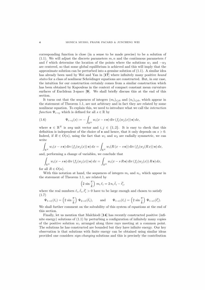
It turns out that the sequences of integers (mi)i≥0 and (ni)i≥0, which appear inthe statement of Theorem 1.1, are not arbitrary and in fact they are related by somenonlinear equation. To explain this, we need to introduce what we call the interactionfunction Ψi→j which is defined for all s ∈ R by
(1.6) Ψi→j(s) := −∫RN
wi(x− s e) div (fj(wj(x)) e) dx,
where e ∈ RN is any unit vector and i, j ∈ 1, 2. It is easy to check that thisdefinition is independent of the choice of e and hence, that it only depends on s > 0.Indeed, if R ∈ O(n), using the fact that w1 and w2 are radially symmetric, we canwrite∫
RNwi(x− s e) div (fj(wj(x)) e) dx =
∫RN
wi(R (x− s e)) div (fj(wj(Rx)) e) dx,
and, performing a change of variables, we conclude that∫RN
wi(x− s e) div (fj(wj(x)) e) dx =
∫RN
wi(x− sR e) div (fj(wj(x))R e) dx,
for all R ∈ O(n).With this notation at hand, the sequences of integers mi and ni, which appear in
the statement of Theorem 1.1, are related by(2 sin
π
k
)mi `i = 2ni ¯
i − ¯′i,
where the real numbers `i, ¯i, ¯′
i > 0 have to be large enough and chosen to satisfy(1.7)
Ψ1→1(`i) =(
2 sinπ
k
)Ψ2→1(¯
i), and Ψ1→1(`i) =(
2 sinπ
k
)Ψ1→1(¯′
i).
We shall further comment on the solvability of this system of equations at the end ofthis section.
Finally, let us mention that Malchiodi [14] has recently constructed positive (infi-nite energy) solutions of (1.1) by perturbing a configuration of infinitely many copiesof the positive solution w1 arranged along three rays meeting at a common point.The solutions he has constructed are bounded but they have infinite energy. Our keyobservation is that solutions with finite energy can be obtained using similar ideasprovided one considers sign-changing solutions and this is precisely the contribution

FINITE-ENERGY SIGN-CHANGING SOLUTIONS 5
of our paper. Let us also mention that positive solutions of (1.1) with unboundedenergy have also been constructed by del Pino, Kowalczyk, Pacard and Wei in [6]again using ideas which steam from similar construction in the theory of non compactconstant mean curvature surfaces of Euclidean 3-space.
The proof of the main result is rather technical and, in order to help allay thecomplexity of the notations and present the main ideas as clearly as possible, we willprove Theorem 1.1 in the case where the nonlinearity is given by
f(u) = |u|p−1 u.
Mutatis mutandis, the proof goes through for any nonlinearity satisfying (H.1)-(H.3).Therefore, from now on, we will be interested in solutions of
(1.8) ∆u− u+ |u|p−1 u = 0,
in RN , which tend to 0 as |x| tends to∞. We will assume that the exponent p satisfies1 < p < N+2
N−2 when N ≥ 3 and 1 < p when N = 2. Observe that equation (1.8) is theEuler-Lagrange equation of the functional defined by
(1.9) E (u) :=1
2
∫RN
(|∇u|2 + u2
)dx− 1
p+ 1
∫RN|u|p+1 dx,
and let us recall that there exists a unique radially symmetric (in fact radially de-creasing) positive solution of
∆w − w + wp = 0,
in RN , which tends to 0 as |x| tends to ∞. Moreover, all positive solutions of (1.8),which tend to 0 at∞, are translates of w. The function w together with its translationswill constitute the building blocks of our construction.
As far as the asymptotic behavior of w at infinity is concerned, it is known thatthere exists a constant cN,p > 0, only depending on N and p, such that
(1.10) limr→∞
er rN−1
2 w = cN,p > 0, and limr→∞
w′
w= −1,
where we have set r := |x|. Of importance to us will be the interaction function Ψdefined by
(1.11) Ψ(s) := −∫RN
w(· − s e) div(wp e) dx,
where e ∈ RN is any unit vector. It is known (see Lemma 5.1) that
Ψ(s) = CN,p e−s s−
N−12 (1 +O(s−1)) as s→∞,
where the constant CN,p > 0 only depends on N and p. Similar estimates hold forthe derivatives of Ψ and in particular, we have
(1.12) −(log Ψ)′(s) = 1 +N − 1
2 s+O(s−2) as s→∞.
Finally, the solution w is nondegenerate in the sense defined in (1.3) (we refer thereader to [15] for a proof of this fact).
6 MONICA MUSSO, FRANK PACARD & JUNCHENG WEI
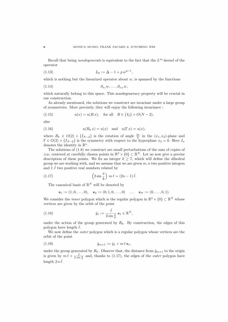
Recall that being nondegenerate is equivalent to the fact that the L∞-kernel of theoperator
(1.13) L0 := ∆− 1 + pwp−1,
which is nothing but the linearized operator about w, is spanned by the functions
(1.14) ∂x1w, . . . , ∂xNw,
which naturally belong to this space. This nondegeneracy property will be crucial inour construction.
As already mentioned, the solutions we construct are invariant under a large groupof symmetries. More precisely, they will enjoy the following invariance :
(1.15) u(x) = u(Rx), for all R ∈ I2 ×O(N − 2),
also
(1.16) u(Rk x) = u(x) and u(Γx) = u(x),
where Rk ∈ O(2) × IN−2 is the rotation of angle 2πk in the (x1, x2)-plane and
Γ ∈ O(2)× IN−2 is the symmetry with respect to the hyperplane x2 = 0. Here Indenotes the identity in Rn.
The solutions of (1.8) we construct are small perturbations of the sum of copies of±w, centered at carefully chosen points in R2 × 0 ⊂ RN . Let us now give a precisedescription of these points. We fix an integer k ≥ 7, which will define the dihedralgroup we are working with, and we assume that we are given m,n two positive integersand `, ¯ two positive real numbers related by
(1.17)(
2 sinπ
k
)m` = (2n− 1) ¯.
The canonical basis of RN will be denoted by
e1 := (1, 0, . . . , 0), e2 := (0, 1, 0, . . . , 0) . . . eN := (0, . . . , 0, 1).
We consider the inner polygon which is the regular polygon in R2×0 ⊂ RN whosevertices are given by the orbit of the point
(1.18) y1 :=¯
2 sin πk
e1 ∈ RN ,
under the action of the group generated by Rk. By construction, the edges of thispolygon have length ¯.
We now define the outer polygon which is a regular polygon whose vertices are theorbit of the point
(1.19) ym+1 := y1 +m` e1,
under the group generated by Rk. Observe that, the distance from ym+1 to the origin
is given by m` +¯
2 sin πk
and, thanks to (1.17), the edges of the outer polygon have
length 2n ¯.

FINITE-ENERGY SIGN-CHANGING SOLUTIONS 7
By construction, the distance between the points y1 and ym+1 is equal to m` andwe will denote by yj , for j = 2, . . . ,m the points evenly distributed on the segmentbetween these two points. Namely
(1.20) yj := y1 + (j − 1) ` e1 for j = 1, . . . ,m.
As already mentioned, the edges of the outer polygon have length 2n ¯ and hence,the distance between the points ym+1 and Rk ym+1 is equal to 2n ¯. Again we dis-tribute evenly points zh, h = 1, . . . , 2n− 1, along this segment. More precisely, if wedefine
(1.21) t := − sinπ
ke1 + cos
π
ke2 ∈ RN ,
then the points zh are given by
(1.22) zh := ym+1 + h ¯t for h = 1, . . . , 2n− 1.
Observe that, by construction
Rk ym+1 = ym+1 + 2n ¯t.
Remark 1.1. — In the general case, namely when the nonlinearity is not odd andhence w1 6= w2, some changes are needed in the definitions of the inner and outerpolygons. In the construction of the inner polygon, ¯ used in (1.18) has to be replacedby ¯′ which is defined in terms of ` by the second equation in (1.7) and ¯ which isused to define the outer polygon is defined by the first equation. Finally, (1.17) whichrelates `, ¯ and ¯′, has to be replaced by(
2 sinπ
k
)m` = 2n ¯− ¯′.
The solutions we construct will be perturbations of the function U which is thesum of positive copies of w centered at the points yj , for j = 1, . . . ,m + 1, togetherwith their images by the rotations Rik = Rk . . . Rk (composition of Rk, i times),for i = 1, . . . , k − 1, and copies of (−1)h w (hence with alternating sign) centered atthe points zh, for h = 1, . . . , 2n − 1, together with their images by the rotations Rik,for i = 1, . . . , k − 1. To be more specific, we define
(1.23) U :=
k−1∑i=0
m+1∑j=1
w(· −Rik yj) +
2n−1∑h=1
(−1)hw(· −Rik zh)
.
So far, the approximate solution U depends on two discrete parameters (the integersm and n) and two continuous parameters (the positive reals ` and ¯) which are related
by (1.17). It should be clear from the construction that the function U we haveconstructed is invariant under the action of Dk ×O(N − 2). Moreover, (1.17) is justa translation of the fact that the length of the rays and the length of the edges of theouter regular polygon are related. The construction of the approximate solution Ualso depends on the parameter k which defines the dihedral group under the actionof which our solution will be invariant. The constraint k ≥ 7 has a purely geometricorigin, roughly speaking, we need π
2 −πk , which is the angle at ym+1 between the edge

8 MONICA MUSSO, FRANK PACARD & JUNCHENG WEI
of the outer regular polygon and the ray joining this vertex to the origin, to be largerthan π
3 . Henceπ
2− π
k>π
3.
In turn, this last condition steams from the maximal number of non overlapping disksof radius 1 which are tangent to a given disc of radius 1 in the plane. As we will see
¯= `+O(1).
Now, let us analyze more carefully the situation at the point ym+1. When k ≤ 6, theangle π
2 −πk <
π3 and hence the copies of w centered at the points ym and z1 interact
too much to consider that U is a good approximate solution to our problem, this isjust a consequence of the fact that the distance between ym and z1 can be estimatedby
2 ` sin(π
4− π
2k
)< `+O(1),
when ` tends to infinity. Therefore, when assuming that k ≥ 7, we ask that the closestneighbors of the point ym are ym, z1 and R−1
k z2n−1. Similarly, we ask that the closestneighbors of the point z1 are ym+1 and z2. A similar analysis can be carried over atthe point y1 and one can check that, when assuming that k ≥ 7, we ask that theclosest neighbors of the point y1 are y2, Ry y1 and R−1
k y1.We now assume that the integer k ≥ 7 is fixed, that m,n are two positive integers
and `, ¯ are two positive real numbers satisfying (1.17). We now further assume that` and ¯ are related by
(1.24) Ψ(`) =(
2 sinπ
k
)Ψ(¯),
where Ψ is the function defined in (1.11). The origin of this second constraint onthe choice of the parameters is not obvious at all. It can either be understood as abalancing condition which is a consequence of a conservation law for solutions of (1.8)(corresponding to the well known balancing formula in the framework of constantmean curvature surfaces) or it can be understood as a condition which will ensurethat the approximate solution we consider is, in a sense to be made precise, very closeto a genuine solution of (1.8) (we refer to §5 where this second equation will arise andto the Appendix, where some formal justification of this constraint will be given).
Then, Theorem 1.1 is a direct consequence of the following result :
Theorem 1.2. — Assume that the integer k ≥ 7 and the real number A > 0 arefixed. There exists a positive constant `0 > 0 such that, for all ` ≥ `0, if ¯ is thesolution of
(1.25) Ψ(`) =(
2 sinπ
k
)Ψ(¯),
if n,m are positive integers satisfying
(1.26)(
2 sinπ
k
)m` = (2n− 1) ¯,
and if
m ≤ `A,

FINITE-ENERGY SIGN-CHANGING SOLUTIONS 9
then (1.8) has a sign changing solution u which satisfies the symmetry conditionsgiven in (1.15) and (1.16). Moreover
(1.27) u = U + o(1),
where o(1)→ 0 uniformly in RN as `→∞, and the energy of u is finite and can beexpanded as
(1.28) E (u) = k (m+ 2n) E (w) + o(1),
where o(1)→ 0 as `→∞.
Remark 1.2. — The condition m ≤ `A is purely technical and is a drawback of ourproof. In fact, going carefully through the last arguments of the proof, it is clear thatthis condition can already be weakened to handle the cases where
m ≤ eA`,for some fixed A > 0, chosen small enough. What is more, we are convinced thatthis condition can be completely removed by choosing different weighted norms on thespaces of functions we are considering (see [8] and [9]). Since this would enlargeconsiderably the size of the paper, we have chosen not to follow this route.
Observe that, once ` is fixed large enough, the constant ¯ is given uniquely by(1.25). Therefore, the existence of solutions of (1.8) depends on our ability to solve(1.26) for some integers m,n. Indeed, it follows from (1.25) that ¯ is implicitly givenas a function of ` (provided this later is large enough) and that it can be expanded,in powers of `, as
(1.29) ¯= `+ ln(
2 sinπ
k
)+O(`−1),
as ` tends to∞. Inserting this information back into (1.26), we find using Lemma 5.1,that (1.26) reduces to
(1.30)2n− 1
m= 2 sin
π
k
(1− ln
(2 sin
π
k
)`−1 +O(`−2)
).
We are now in a position to give examples of such solutions. Certainly, for anyinteger m ≥ 1, one can choose n ∈ N such that
(1.31) 1 ≤ 2n− 1−(
2 sinπ
k
)m < 3.
Then, provided m is chosen large enough, there will exist a unique ` > `0 satisfying(1.26) and (1.31), together with (1.30), implies that there exist positive constantsC1 < C2 such that
(1.32) C1m ≤ ` ≤ C2m.
Theorem 1.2 then ensures the existence of solutions of (1.8) for each such a choice ofthe integer m.
To complete the description of our construction, let us briefly comment on therelation between this result and the corresponding construction for constant meancurvature surfaces in Euclidean 3-space. As already mentioned, the constructionin the present paper follows very closely a similar construction of compact constant

10 MONICA MUSSO, FRANK PACARD & JUNCHENG WEI
mean curvature surfaces given in [9]. In this framework one tries to construct compactconstant mean curvature surfaces in Euclidean 3-space by connecting together spheresof radius 1 which are tangent. In the initial configuration, the center of the spherescan be arranged along the edges of a very large regular polygon and also along the raysjoining the center to the vertices of the polygon. It is proven in [9] that a perturbationargument can be applied and, as a result, a compact constant mean curvature surfaceis obtained (provided the size of the polygon is large enough). This surface can beconstructed in such a way that the pieces which are close to the rays joining the originto the vertices are embedded and close to embedded constant mean curvature surfaceswhich are known as unduloıds, while the pieces which are close to the edges of theregular polygon are immersed constant mean surfaces which are close to nodoıds (inour framework, this corresponds to the fact that we arrange solutions with the samesign along the rays joining the origin to the vertices of the polygon and solutions withalternative sign along the edges of the polygon). A similar construction has also beenobtained by Jleli and Pacard in [8].
Remark 1.3. — For the sake of simplicity, we have chosen to present the proof ofthe existence of solutions which are invariant under the action of a rather large groupof symmetry. However, a more general construction (i.e. leading to solutions of (1.8)having less symmetry) can be obtained as is the case for constant mean curvaturesurfaces [9], we shall address this problem in a forthcoming paper.
In the next section, we describe more carefully the solution predicted in the aboveTheorem and we give an overview of the proof and of the plan of the paper.
Acknowledgments : The authors would like to thank the referee for valuablecomments which help improving some of the arguments of the paper.
2. Ansatz and sketch of the proof
We construct a finite dimensional family of approximate solutions of (1.8) which are
close to U and depend on 2n+m parameters which we now define. These approximatesolutions are in fact equal to U when all the parameters are set to 0. This time, insteadof centering the copies of ±w at the points yj , zh as well as at their images by therotations Rik, for i = 1, . . . , k − 1, we center the copies of ±w at points which aresmall perturbations of the points yj , zh. To make this precise, we define
(2.1) yj := yj + αj e1, for j = 1, . . . ,m+ 1,
and
(2.2) zh := zh + βh t + ¯γh n, for h = 1, . . . , 2n− 1,
where ¯ has been defined in (1.24), t has been defined in (1.21) and
n := cosπ
ke1 + sin
π
ke2.
Observe that, since we assume that our construction is invariant under the dihedralgroup of symmetry generated by Γ and Rk (see (1.16), the points zh and z2n−h are

FINITE-ENERGY SIGN-CHANGING SOLUTIONS 11
related by
z2n−h = Rk(Γ zh),
for all h = 1, . . . , n. In other words, if we rotate by the rotation Rk the point obtainedby reflecting zh with respect to the plane x2 = 0 we get z2n−h. Since Rk(Γ t) = −tand Rk(Γ n) = n, this implies that we necessarily have
(2.3) βh = −β2n−h and γh = γ2n−h,
for h = 1, . . . , n and in particular βn = 0. We thus conclude that there are only2n+m free parameters.
We will assume that the parameters which appear in the definition of both yj andzh satisfy
(2.4)
|αj | ≤ 1, for j = 1, . . . ,m+ 1
|βh| ≤ 1, for h = 1, . . . , n− 1
` |γh| ≤ 1, for h = 1, . . . , n.
In these inequalities, the constant 1 is arbitrary and can be replaced by any positiveconstant.
The set of points where the copies of w will be centered is now given by
(2.5) Π :=
k−1⋃i=0
(Rik yj : j = 1, . . . ,m+ 1 ∪ Rik zh : h = 1, . . . , 2n− 1
),
and we now look for a solution of (1.8) of the form u = U + φ, where
(2.6) U(x) :=
k−1∑i=0
m+1∑j=1
w(x−Rik yj) +
2n−1∑h=1
(−1)hw(x−Rik zh)
.
Observe that, by construction, the function U satisfies the symmetry assumption(1.15) and (1.16). We define
(2.7) L := ∆− 1 + p |U |p−1,
(2.8) E := |U |p−1 U −k−1∑i=0
m+1∑j=1
wp(· −Rik yj) +
2n−1∑h=1
(−1)hwp(· −Rik zh)
,
and
(2.9) Q(φ) := |U + φ|p−1(U + φ)− |U |p−1U − p |U |p−1 φ.
Observe that both E and Q depend implicitly on the parameters αj , βh and γh eventhough this is not apparent in the notations. With these notations, the solvability of(1.8) reduces to find parameters αj , βh and γh and a function φ which are solutionsof the nonlinear problem
(2.10) Lφ+ E +Q(φ) = 0,
in RN and which tends to 0 as |x| tends to ∞.

12 MONICA MUSSO, FRANK PACARD & JUNCHENG WEI
Remark 2.1. — We will solve (2.10) in the class of functions φ satisfying (1.15)and (1.16). Therefore, from now on, we always assume that all the functions weconsider satisfy (1.15) and (1.16) without further mentioning it.
In order to solve this highly nonlinear problem, we apply a Liapunov-Schmidt typereduction argument : first, we solve a projected problem which allows one to reducethe solvability of (2.10) to the solvability of some finite dimensional nonlinear system(called the reduced problem), then, in a second step, we will explain how to solve thereduced problem.
To proceed, we assume that the real numbers `, ¯ are chosen so that (1.24) holdsand that integers n and m satisfy (1.17). We consider a cut off function χ ∈ C∞(R)such that
(2.11)
χ(s) ≡ 1 for s ≤ −1,
χ(s) ≡ 0 for s ≥ 0.
We fix a constant ζ > 0 (independent of ` and the choice of the parameters αj , βh and
γh satisfying the constraints (2.4)) so that the balls of radius `−ζ2 , centered at different
points of Π are mutually disjoint, for all ` large enough. This is possible thanks to(1.29) and our geometric assumption (namely k ≥ 7) which implies that the minimumdistance between two different points of Π is bounded from below by `− ζ0 for someconstant ζ0 > 0 independent of ` large enough (say ` ≥ `0). Observe that, whenk ≤ 6 the distance between ym and z1 can be evaluated by 2 sin(π4 −
π2k ) `+O(1), as
` tends to ∞ and therefore a proper choice of ζ would not have been possible in thiscase since 2 sin(π4 −
π2k ) < 1. We define the compactly supported vector field
(2.12) Ξ(x) := χ (2 |x| − `+ ζ) ∇w(x).
Observe that, by construction (in fact given the choice of ζ), we have, for all y, z ∈ Π
(2.13)
∫RN
(ei · Ξ(· − y)) (ej · Ξ(· − z)) dx = 0,
if i 6= j or if y 6= z.It will be convenient to define the function
(2.14) M(c, d) :=
k−1∑i=0
m+1∑j=1
Rik cj · Ξ(· −Rik yj) +
2n−1∑h=1
Rik dh · Ξ(· −Rik zh)
,
as well as the operator
(2.15) L(φ, c, d) := Lφ+M(c, d),
where φ is a function defined on RN , the (m+ 1)-tuple
c := (c1, . . . , cm+1) ∈ (R e1)m+1,
and the (2n− 1)-tuple
d := (d1, . . . , d2n−1) ∈ (R e1 ⊕ R e2)2n−1.

FINITE-ENERGY SIGN-CHANGING SOLUTIONS 13
Observe that, given the symmetries we impose to all the functions we deal with (seeRemark 2.1), the function M(c, d) has to be invariant under the action of both Rkand Γ and this implies that, for h = 1, . . . , n, the vectors dh and d2n−h are related by
d2n−h = Rk(Γ dh),
and hence d2n−h can be expressed in terms of dh as
d2n−h = −(dh · t) t + (dh · n) n.
In the next section, we will define suitable function spaces in which the equation
(2.16) L (φ, c, d) = h,
in RN , admits a solution which tends to 0 as |x| tends to ∞ and which satisfies theorthogonality condition
(2.17)
∫RN
φ e1 · Ξ(· − yj) dx = 0,
for j = 1, . . . ,m+ 1, and
(2.18)
∫RN
φ ei · Ξ(· − zh) dx = 0,
for h = 1, . . . , n and i = 1, 2. Again, given the symmetries we impose to all thefunctions we deal with (see Remark 2.1), a function φ satisfies (2.17) and (2.18) ifand only if it satisfies
(2.19)
∫RN
φ ei · Ξ(· − y) dx = 0,
for all i = 1, . . . , N and all y ∈ Π.In order to study the operator L, the key idea is that the linear operator L is close
to be the sum of many copies of
L0 = ∆− 1 + pwp−1,
centered at the points of Π and we take advantage from the fact that the invertibilityof L0 is well understood.
Once the linear theory is understood, we will consider the following nonlinear pro-jected problem : given the points yj and zh defined in (2.1), (2.2) and satisfying (2.4),find a function φ, satisfying the symmetry assumptions (1.15), (1.16), the orthogonal-ity conditions (2.17) and (2.18) and tending to 0 as |x| tends to ∞ and find vectorscj , dh such that
(2.20) L (φ, c, d) + E +Q(φ) = 0,
in RN .In the next sections, we show unique solvability of (2.20) by means of a fixed point
argument and we prove that the solution φ depends continuously (and in fact, withmore work one can prove that the solution φ depends smoothly on the points yj andzh). To achieve this, we first study the solvability of a linear problem and then applysome standard fixed point theorem for contraction mapping to solve the nonlinearproblem.

14 MONICA MUSSO, FRANK PACARD & JUNCHENG WEI
3. Linear theory
The main result of this section is concerned with the solvability of (2.16), uniformlyin `, as ` tends to ∞, and also in the parameters αj , βh and γh satisfying the con-straints (2.4). We henceforth assume that the real numbers `, ¯ are chosen so that(1.24) holds and that integers n and m satisfy (1.17). In particular,
¯= `+O(1).
We prove that, provided ` is large enough, the linear operator L defined in the previoussection in (2.15) has nice mapping properties.
Given η < 0, we consider the weighted norm
(3.1) ‖h‖∗ := supx∈RN
∣∣∣∣∣∣∣∑y∈Π
eη |x−y|
−1
h(x)
∣∣∣∣∣∣∣ ,where we recall that the set of points Π was defined in (2.5).
With this definition at hand, we prove the following a priori estimate :
Lemma 3.1. — Assume that η < 0 is fixed. There exist `0 > 0, δ0 > 0 and C > 0(all depending on the choice of η) such that, for all ` > `0, the following inequalityholds
supi=1,...,m+1
|ci|+ suph=1,...,n
|dh| ≤ C(‖L(φ, c, d)‖∗ + e−δ0` ‖φ‖∗
).
Observe that the estimate does not depend on n and m, nor on ` provided thislatter is chosen large enough. further observe that
suph=1,...,n
|dh| = suph=1,...,2n−1
|dh|,
since d2n−h = dh, for h = 1, . . . , n.
Proof. — Let us give a detailed proof of the estimate of the coefficient c1. We startwith the definition of L given in (2.15) which we multiply by e1 · Ξ(· − y1). Usingsome integration by parts together with (2.13), we obtain
c1 · e1
∫RN
(e1 · Ξ(· − y1))2 dx =
∫RNL(φ, c, d) (e1 · Ξ(· − y1)) dx
−∫RN
φL (e1 · Ξ(· − y1)) dx.
Obviously,
lim`→∞
∫RN
(e1 · Ξ(· − y1))2 dx =1
N
∫RN|∇w|2 dx,
therefore ∫RN
(e1 · Ξ(· − y1))2 dx ≥ C0 > 0,

FINITE-ENERGY SIGN-CHANGING SOLUTIONS 15
for all ` large enough (say ` > `0). Thanks to (1.10), we know that |Ξ| is boundedand hence we can estimate∣∣∣∣∫
RNL(φ, c, d) (e1 · Ξ(· − y1)) dx
∣∣∣∣ ≤ C ‖L(φ, c, d)‖∗,
provided ` > `0. Finally, since
L0(e1 · ∇w) =(∆− 1 + pwp−1
)(e1 · ∇w) = 0,
we can write
L (e1 · Ξ(· − y1)) = L (e1 · Ξ(· − y1))− L0(e1 · ∇w(· − y1))
and, using this, it is easy to check that there exists a constant C > 0 and δ0 > 0 suchthat ∣∣∣∣∫
RNφL (e1 · Ξ(· − y1)) dx
∣∣∣∣ ≤ C e−δ0` ‖φ‖∗,where δ0 > 0 depends on η < 0. To obtain the last estimate, two different effects haveto be taken into account : the first one is the effect of the Laplace operator on thecutoff function χ which is used to define Ξ and the second one is the difference betweenthe two potentials p |U |p−1 and pwp−1 which appear respectively in the definition ofL and L0. The proof of the estimate for c1 follows at once from the above estimates.A similar proof holds for the estimates of any cj and any dh. We leave the details tothe reader.
Thanks to the previous estimate, we can prove the following :
Proposition 3.1. — Assume that η ∈ (−1, 0) is fixed. There exist `0 > 0 and C > 0such that, for all ` > `0, the following inequality holds
(3.2) ‖φ‖∗ ≤ C ‖L(φ, c, d)‖∗,provided φ satisfies (2.17) and (2.18).
Again, it is worth mentioning that the estimate does not depend on n and m, noron ` provided this latter is chosen large enough.
Proof. — To begin with, we make use of the result of the previous Lemma togetherwith the fact that |Ξ| is bounded by a constant times e−|x|. This later fact follows atonce from (1.10). Since we assume that η ∈ (−1, 0), we conclude that(3.3)
‖M(c, d)‖∗ ≤ C
(sup
i=1,...,m+1|ci|+ sup
h=1,...,n|dh|
)≤ C
(‖L(φ, c, d)‖∗ + e−δ0` ‖φ‖∗
),
for some constant C > 0, which does not depend on ` > `0.It is easy to check that the function
W :=∑y∈Π
eη |·−y|,
satisfies
LW ≤ − (1− η2)
2W,

16 MONICA MUSSO, FRANK PACARD & JUNCHENG WEI
in RN \ ∪y∈ΠB(y, ρ) provided ρ is fixed large enough (independently of ` ≥ `0).Indeed, for all y ∈ Π, we can write
Leη|x−y| = −(
1− η2 − N − 1
|x− y|η − p |U |p−1
)eη|x−y| ≤ − (1− η2)
2eη|x−y|,
provided dist(x,Π) is large enough, since |U |p−1 tends to 0 away from the points ofΠ.
Making use of the fact that that η ∈ (−1, 0) together with the maximum principle,we conclude that the function W can be used as a barrier to prove the pointwiseestimate
(3.4) |φ|(x) ≤ C(‖Lφ‖∗ + sup
y∈Π‖φ‖L∞(∂B(y,ρ))
)W (x),
for all x ∈ RN \ ∪y∈ΠB(y, ρ).Granted this preliminary estimate, the proof of the result goes by contradiction.
Let us assume there exist a sequence of ` tending to ∞ and a sequence of solutions of(2.16) for which the inequality is not true. The problem being linear, we can reduceto the case where we have a sequence `(i) tending to ∞ and sequences φ(i), c(i), d(i)
such that
‖L(φ(i), c(i), d(i))‖∗ −→ 0, and ‖φ(i)‖∗ = 1.
But (3.3) implies that we also have ‖M(c(i), d(i))‖∗ −→ 0 and hence
‖Lφ(i)‖∗ −→ 0.
Then, (3.4) implies that there exists y(i) ∈ Π such that
(3.5) ‖φ(i)‖L∞(B(y(i),ρ)) ≥ C,
for some fixed constant C > 0. Using elliptic estimates together with Ascoli-Arzela’stheorem, we can find a sequence y(i) and we can extract, from the sequence φ(i)(·−y(i))a subsequence which converges (uniformly on compact sets) to φ∞ which is a solutionof (
∆− 1 + pwp−1)φ∞ = 0,
in RN and which is bounded by a constant times eη |x|, with η < 0. Moreover, recallthat φ(i) satisfies the orthogonality conditions (2.17) and (2.18) and also satisfiessome symmetry properties which are described in Remark 2.1 (and in particular, thisimplies that φ(i) satisfies (2.19)). Using this and passing to the limit, one checks thatthe limit function φ∞ also satisfies∫
RNφ∞ ∂xjw dx = 0,
for j = 1, . . . , N . But the solution w being non degenerate, this implies that φ∞ ≡ 0,which is certainly in contradiction with (3.5), which implies that φ∞ is not identicallyequal to 0.
Having reached a contradiction, this completes the proof of the Proposition.
We are now in a position to prove the main result of this section :

FINITE-ENERGY SIGN-CHANGING SOLUTIONS 17
Proposition 3.2. — Assume that η ∈ (−1, 0) is fixed. There exist `0 > 0 and C > 0such that, for all ` > `0, and for all h ∈ L∞(RN ) satisfying ‖h‖∗ <∞, there exists aunique triple (φ, c, d) solution of
L (φ, c, d) = h,
in RN , such that φ satisfies (2.17) and (2.18). Moreover
(3.6) supi=1,...,m+1
|ci|+ suph=1,...,n
|dh|+ ‖φ‖∗ ≤ C ‖h‖∗.
As in the previous results, it is important to notice that the estimate does notdepend on the integers n and m, nor on ` provided this latter is chosen large enough.
Proof. — We consider the Hilbert space
H =
φ ∈ H1(RN ) :
∫RN
φ e · Ξ(· − y) dx = 0, ∀y ∈ Π, ∀e ∈ RN , |e| = 1
,
and, as usual, we also assume that the functions enjoy the symmetries described inRemark 2.1.
Assume that we are given h ∈ L2(RN ). Standard arguments (i.e. Lax-Milgram’sTheorem) imply that
φ ∈ H 7−→ 1
2
∫RN
(|∇φ|2 + φ2) dx+
∫RN
φh dx,
has a unique minimizer φ ∈ H (here we implicitly use the fact that η < 0 so thatthe last term is a continuous linear functional defined in H). Then, φ is the unique aweak solution of
∆φ− φ− h ∈ Span
k−1∑i=0
Rike1 · Ξ(· −Rikyj) : j = 1, . . . ,m+ 1
⊕
Span
k−1∑i=0
Rikej · Ξ(· −Rikzh) : j = 1, 2 , h = 1, . . . , n
,
which belongs to H. In other words, if we define the operator
L0(φ, c, d) := ∆φ− φ+M(c, d),
we have uniquely solved
L0(φ, c, d) = h,
for φ ∈ H, cj ∈ R e1 and dh ∈ Re1 ⊕ Re2. Thanks to the above arguments
L−10 : L2(RN ) 7−→ H× (R e1)m+1 × (R e1 ⊕ R e2)2n−1,
is well defined.The solvability of
L(φ, c, d) = h,
in H× (R e1)m+1× (R e1⊕R e2)2n−1 can then by rephrased in the invertibility of theoperator I +K, where by definition
(3.7) K(φ, c, d) := L−10 (p |U |p−1 φ).
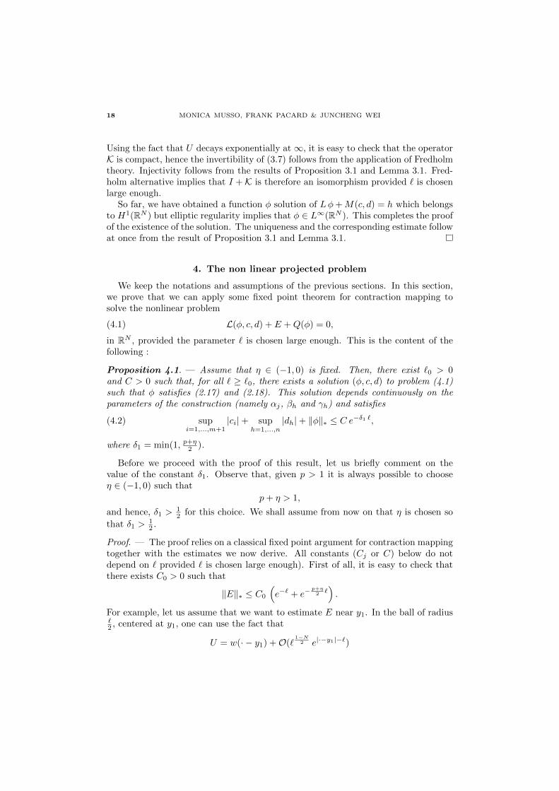
18 MONICA MUSSO, FRANK PACARD & JUNCHENG WEI
Using the fact that U decays exponentially at∞, it is easy to check that the operatorK is compact, hence the invertibility of (3.7) follows from the application of Fredholmtheory. Injectivity follows from the results of Proposition 3.1 and Lemma 3.1. Fred-holm alternative implies that I +K is therefore an isomorphism provided ` is chosenlarge enough.
So far, we have obtained a function φ solution of Lφ+M(c, d) = h which belongsto H1(RN ) but elliptic regularity implies that φ ∈ L∞(RN ). This completes the proofof the existence of the solution. The uniqueness and the corresponding estimate followat once from the result of Proposition 3.1 and Lemma 3.1.
4. The non linear projected problem
We keep the notations and assumptions of the previous sections. In this section,we prove that we can apply some fixed point theorem for contraction mapping tosolve the nonlinear problem
(4.1) L(φ, c, d) + E +Q(φ) = 0,
in RN , provided the parameter ` is chosen large enough. This is the content of thefollowing :
Proposition 4.1. — Assume that η ∈ (−1, 0) is fixed. Then, there exist `0 > 0and C > 0 such that, for all ` ≥ `0, there exists a solution (φ, c, d) to problem (4.1)such that φ satisfies (2.17) and (2.18). This solution depends continuously on theparameters of the construction (namely αj, βh and γh) and satisfies
(4.2) supi=1,...,m+1
|ci|+ suph=1,...,n
|dh|+ ‖φ‖∗ ≤ C e−δ1 `,
where δ1 = min(1, p+η2 ).
Before we proceed with the proof of this result, let us briefly comment on thevalue of the constant δ1. Observe that, given p > 1 it is always possible to chooseη ∈ (−1, 0) such that
p+ η > 1,
and hence, δ1 >12 for this choice. We shall assume from now on that η is chosen so
that δ1 >12 .
Proof. — The proof relies on a classical fixed point argument for contraction mappingtogether with the estimates we now derive. All constants (Cj or C) below do notdepend on ` provided ` is chosen large enough). First of all, it is easy to check thatthere exists C0 > 0 such that
‖E‖∗ ≤ C0
(e−` + e−
p+η2 `).
For example, let us assume that we want to estimate E near y1. In the ball of radius`2 , centered at y1, one can use the fact that
U = w(· − y1) +O(`1−N
2 e|·−y1|−`)

FINITE-ENERGY SIGN-CHANGING SOLUTIONS 19
to expand E as
|E| =∣∣∣(w(· − y1) +O(`
1−N2 e|·−y1|−`)
)p− wp(· − y1) +O(`p
1−N2 ep(|·−y1|−`))
∣∣∣≤ C e(2−p)|·−y1|−`
≤ C(e−` + e−
p+η2 `)eη |·−y1|
≤ C(e−` + e−
p+η2 `) ∑y∈Π
eη |·−y|.
Away from the balls of radius `2 centered at the points of Π, we take advantage from
the fact that U decays exponentially to prove that
|E| ≤ C∑y∈Π
e−p |·−y| ≤ C e−p+η2 `
∑y∈Π
eη |·−y|.
The estimate for E then follows at once.We chose δ1 = min(1, p+η2 ) and we set
C1 :=4C0
‖L−1‖.
where L−1 is the inverse of L which has been obtained in Proposition 3.2. Taylor’sexpansion implies that there exist δ2 > 0 and C2 > 0 such that
‖Q(φ1)−Q(φ2)‖∗ ≤ C2 e−δ2 ` ‖φ1 − φ2‖∗,
for all φ1, φ2 satisfiying ‖φj‖∗ ≤ C1 e−δ1 `. Some care is needed to derive the last
estimate. Essentially, the estimate follows from the observation that either one triesto get the estimate at a point where |φ1| + |φ2| ≤ |U |/2, in which case one can usethe inequality
|Q(φ2)−Q(φ1)| ≤ C |U |p−2 (|φ1|+ |φ2|) |φ2 − φ1|,or one tries to get the estimate at a point where |φ1| + |φ1| ≥ |U |/2, in which caseone can use the inequality
|Q(φ2)−Q(φ1)| ≤ C (|φ1|p−1 + |φ2|p−1)|φ2 − φ1|.We leave the details to the reader.
The result of Proposition 3.2 allows one to rewrite (4.1) as a fixed point problem
(φ, c, d) = −L−1 (E +Q(φ)) .
Provided ` is chosen large enough, the above estimates readily yield the existence of aunique fixed point in the ball of radius C1 e
−δ1 ` in the space L∞∗ (RN )× (R e1)m+1 ×(R e1 ⊕ R e2)2n−1, where
L∞∗ (RN ) := φ ∈ L∞(RN ) : ‖φ‖∗ <∞,which is endowed with the norm ‖ · ‖∗ and (R e1)m+1 and (R e1 ⊕ R e2)2n−1 areendowed with the natural norms, namely
‖c‖ := supj=1,...,m+1
|cj |,

20 MONICA MUSSO, FRANK PACARD & JUNCHENG WEI
and
‖d‖ := suph=1,...,n
|dh| = suph=1,...,2n−1
|dh|.
This completes the proof of the existence of a solution of (4.1).Observe that elliptic estimates imply that the solution we have obtained also sat-
isfies
(4.3) ‖φ‖∗ + ‖∇φ‖∗ + ‖∇2φ‖∗ ≤ C3 e−δ1`,
for some constant C3 > 0.It remains to check that the solution we have obtained depends continuously on
the parameters of our construction, namely the parameters αj , δh and γh. Usually,verifying this property is stadard but here, some care is due since the dependence ofthe nonlinear operator on the parameters is quite intricate and not explicit. Indeed,the parameters appear in the definition of L and also in the definition of the functionspace H and hence they implicitly appear in the construction of L−1.
Now, assume that we have two solutions corresponding to two sets of parameters.Say
Lφ+M(c, d) + E +Q(φ) = 0,
corresponding to the points yj and zh and
L φ+ M(c, d) + E + Q(φ) = 0,
corresponding to the points yj and zh (we will adorn all functions and operators with
a ˙ when they correspond to the points yj and zh). Observe that, by construction, φ
is L2-orthogonal to ej · Ξ while φ is L2-orthogonal to ej ·Ξ. First, we choose γ and δso that
˙φ := φ−M(γ, δ) ,
satisfies the same orthogonality condition as the function φ (namely, such that it is a
function L2-orthogonal to Ξ). Then, we rewrite the equation satisfied by φ as
L ˙φ+M(c, d) + (L− L) φ+ L(M(γ, δ)) + (M(c, d)−M(c, d)) + E + Q(φ) = 0.
Taking the difference with the first equation, we get
L (φ− ˙φ, c− c, d− d) = (L− L) φ+ L(M(γ, δ)) + (M(c, d)−M(c, d))
+ (E − E) + (Q(φ)−Q(φ)) + (Q(φ)−Q(φ)).
Using the arguments we have already used to prove the existence of a solution togetherwith (4.3), it is easy to check that there exists δ3 > 0 such that
‖φ− ˙φ‖∗ + ‖c− c‖+ ‖d− d‖ ≤ C e−δ3 ` (supj |yj − yj |+ suph |zh − zh|)
+ C e−δ3 ` (‖γ‖+ ‖δ‖) + C e−δ3` ‖ ˙φ− φ‖∗.
Moreover, we also have the estimate
‖γ‖+ ‖δ‖ ≤ C ‖φ‖∗ (supj|yj − yj |+ sup
h|zh − zh|),
FINITE-ENERGY SIGN-CHANGING SOLUTIONS 21
and hence, we conclude that
‖φ− ˙φ‖∗ + ‖c− c‖+ ‖d− d‖ ≤ C e−δ3 ` (supj|yj − yj |+ sup
h|zh − zh|),
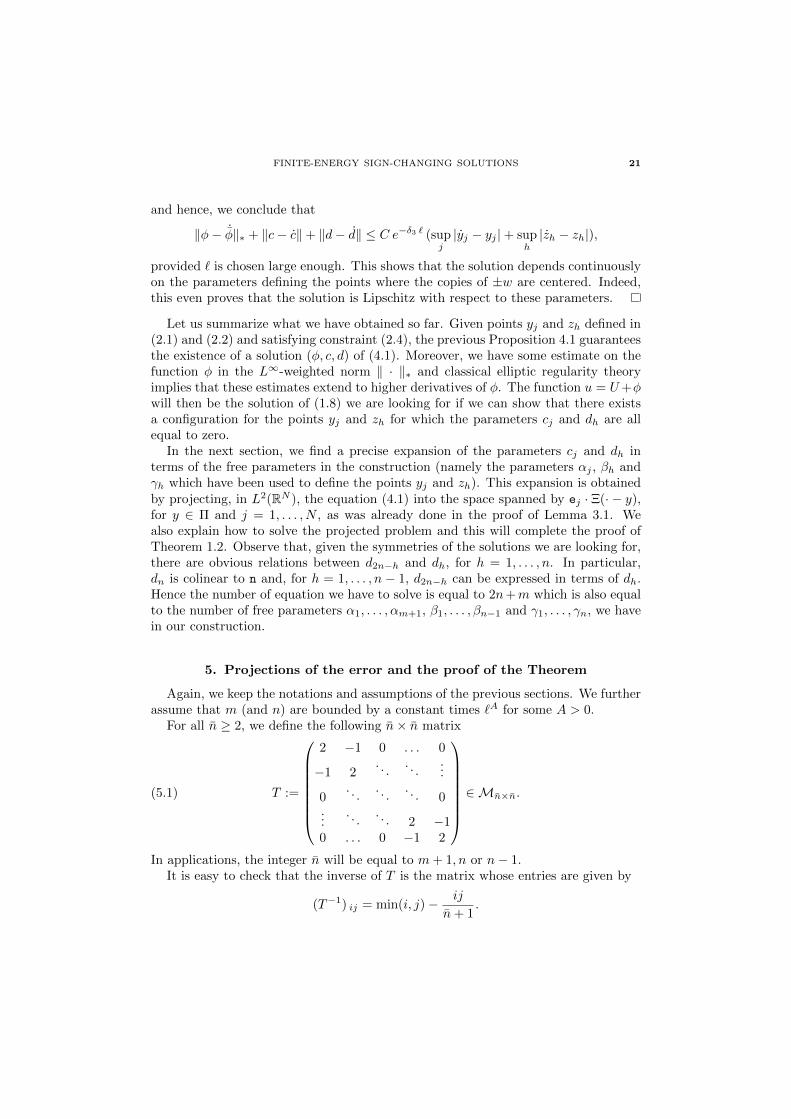
provided ` is chosen large enough. This shows that the solution depends continuouslyon the parameters defining the points where the copies of ±w are centered. Indeed,this even proves that the solution is Lipschitz with respect to these parameters.
Let us summarize what we have obtained so far. Given points yj and zh defined in(2.1) and (2.2) and satisfying constraint (2.4), the previous Proposition 4.1 guaranteesthe existence of a solution (φ, c, d) of (4.1). Moreover, we have some estimate on thefunction φ in the L∞-weighted norm ‖ · ‖∗ and classical elliptic regularity theoryimplies that these estimates extend to higher derivatives of φ. The function u = U+φwill then be the solution of (1.8) we are looking for if we can show that there existsa configuration for the points yj and zh for which the parameters cj and dh are allequal to zero.
In the next section, we find a precise expansion of the parameters cj and dh interms of the free parameters in the construction (namely the parameters αj , βh andγh which have been used to define the points yj and zh). This expansion is obtainedby projecting, in L2(RN ), the equation (4.1) into the space spanned by ej · Ξ(· − y),for y ∈ Π and j = 1, . . . , N , as was already done in the proof of Lemma 3.1. Wealso explain how to solve the projected problem and this will complete the proof ofTheorem 1.2. Observe that, given the symmetries of the solutions we are looking for,there are obvious relations between d2n−h and dh, for h = 1, . . . , n. In particular,dn is colinear to n and, for h = 1, . . . , n − 1, d2n−h can be expressed in terms of dh.Hence the number of equation we have to solve is equal to 2n+m which is also equalto the number of free parameters α1, . . . , αm+1, β1, . . . , βn−1 and γ1, . . . , γn, we havein our construction.
5. Projections of the error and the proof of the Theorem
Again, we keep the notations and assumptions of the previous sections. We furtherassume that m (and n) are bounded by a constant times `A for some A > 0.
For all n ≥ 2, we define the following n× n matrix
(5.1) T :=
2 −1 0 . . . 0
−1 2. . .
. . ....
0. . .
. . .. . . 0
.... . .
. . . 2 −10 . . . 0 −1 2
∈Mn×n.
In applications, the integer n will be equal to m+ 1, n or n− 1.It is easy to check that the inverse of T is the matrix whose entries are given by
(T−1) ij = min(i, j)− ij
n+ 1.

22 MONICA MUSSO, FRANK PACARD & JUNCHENG WEI
We define the vectors S↓ and S↑ by
(5.2) T S↑ := (1, 0, . . . , 0)t ∈ Rn, T S↓ := (0, . . . , 0, 1)t ∈ Rn,
where the superscript t is the transpose so that these are identified with columnmatrices. We have explicitly
S↑ :=1
n+ 1(n, n− 1, . . . , 2, 1)t and S↓ :=
1
n+ 1(1, 2, . . . , n− 1, n)t.
It will be convenient to adopt the following notations
α := (α1, . . . , αm+1)t,
β := (β1, . . . , βn−1)t
γ := (γ1, . . . , γn)t,
where αj , βh and γh are the parameters involved in the construction of the points yjand zh which were given in (2.1) and (2.2). As usual, we assume that these parameterssatisfy (2.4).
As in the introduction (see (1.6)), we define the interaction function
(5.3) Ψ(s) := −∫RN
w(· − s e) div(wp e) dx
where e ∈ RN is a unit vector. The proof of our result is based on the following keyLemma :
Lemma 5.1. — There exists a constant CN,p > 0 only depending on N and p suchthat, the following expansion holds
Ψ(s) := CN,p e−s s−
N−12 (1 +O(s−1)),
as s > 0 tends to infinity.
The proof of the above result is by now standard, we refer to [14] and [12] fordetails.
Finally, we define the numbers
κ := −(log Ψ)′(`), and κ := −(log Ψ)′(¯),
as well as
λ1 := 1− 2κ
κsin
π
kand λ2 := 1 +
κ
κsin
π
k− ¯−1 1
κcot
π
kcos
π
k.
Observe that all these numbers depend on `, ¯,m and n but they converge to limitsas ` tends to infinity. In fact, according to (1.12), we have
lim`−→∞
κ = lim`−→∞
κ = 1
and
lim`−→∞
λ1 = 1− 2 sinπ
k, and lim
`−→∞λ1 = 1 + sin
π
k.
The main result of this section is the proof of the following :

FINITE-ENERGY SIGN-CHANGING SOLUTIONS 23
Proposition 5.1. — Let φ be the solution of (4.1) which has been obtained in Propo-sition 4.1. The coefficients cj and dh are all equal to 0 if and only if the column vectorsα ∈ Rm+1, β ∈ Rn−1 and γ ∈ Rn are solutions of the following nonlinear system
(5.4)
α = λ1 α1 S↑ +
(κ
κβ1 +
1
κcot
π
kγ1 + λ2 αm+1
)S↓ + e−δ2`Bα +Dα,
β = − sinπ
kαm+1 S
↑ + e−δ2`Bβ +Dβ ,
¯γ = cosπ
kαm+1 S
↑ + ¯γn S↓ + e−δ2`Bγ +Dγ ,
where δ2 > 0, B• := B•(`,m, n;α, β, γ) and D• := D•(`,m, n;α, β, γ) denote smoothvector valued functions, whose Taylor expansion in α, β and γ has coefficients whichare uniformly bounded as ` → ∞, provided α, β and γ satisfy (2.4). Moreover, TheTaylor expansions of D• with respect to α, β, γ do not involve any constant nor anylinear term.
The proof of this Proposition relies on the following technical Lemmas. First, usingelementary geometry, we find that :
Lemma 5.2. — The following expansions hold
1
Ψ(`)
∫RN
Ξ(· − y1)E dx =(κ (α2 − α1)− 2 sin
π
kκ α1
)e1 + e−δ3`B +D,
and, for j = 2, . . . ,m,
1
Ψ(`)
∫RN
Ξ(· − yj)E dx = κ (αj−1 − 2αj + αj+1) e1 + e−δ3`B +D,
1
Ψ(`)
∫RN
Ξ(· − ym+1)E dx =(κ (αm − αm+1) + κ
(β1 + sin
π
kαm+1
)+ cot
π
k
(γ1 − ¯−1 cos
π
kαm+1
))e1 + e−δ3`B +D.
We also have
1
Ψ(¯)
∫RN
Ξ(· − z1)E dx = κ(
2β1 − β2 + sinπ
kαm+1
)t
+
(γ2 − 2 γ1 +
1¯ cos
π
kαm+1
)n + e−δ3`B +D,
and
(−1)h
Ψ(¯)
∫RN
Ξ(· − zh)E dx = κ (βh−1 − 2βh + βh+1) t
− (γh−1 − 2γh + γh+1) n + e−δ3`B +D,
for all h = 2, . . . , n− 1, and finally
(−1)n
Ψ(¯)
∫RN
Ξ(· − zn)E dx = 2 (γn − γn−1) n + e−δ3`B +D,
24 MONICA MUSSO, FRANK PACARD & JUNCHENG WEI
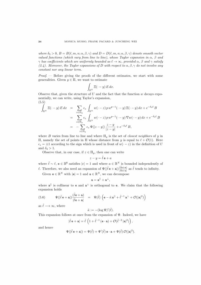
where δ3 > 0, B = B(`,m, n;α, β, γ) and D = D(`,m, n;α, β, γ) denote smooth vectorvalued functions (which vary from line to line), whose Taylor expansion in α, β andγ has coefficients which are uniformly bounded as `→∞, provided α, β and γ satisfy(2.4). Moreover, the Taylor expansions of D with respect to α, β, γ do not involve anyconstant nor any linear term.
Proof. — Before giving the proofs of the different estimates, we start with somegeneralities. Given y ∈ Π, we want to estimate∫
RNΞ(· − y)E dx.
Observe that, given the structure of U and the fact that the function w decays expo-nentially, we can write, using Taylor’s expansion,(5.5)∫
RNΞ(· − y)E dx =
∑z∈Πy
εz
∫RN
w(· − z) pwp−1(· − y) Ξ(· − y) dx+ e−δ4`B
=∑z∈Πy
εz
∫RN
w(· − z) pwp−1(· − y)∇w(· − y) dx+ e−δ4`B
= −∑z∈Πy
εz Ψ(|z − y|) z − y|z − y|
+ e−δ4`B,
where B varies from line to line and where Πy is the set of closest neighbors of y inΠ, namely the set of points in Π whose distance from y is equal to ` + O(1). Hereεz = ±1 according to the sign which is used in front of w(· − z) in the definition of Uand δ4 > 1.
Observe that, in our case, if z ∈ Πy, then one can write
z − y = ˜e + a
where ˜∼ `, e ∈ RN satisfies |e| = 1 and where a ∈ RN is bounded independently of
`. Therefore, we also need an expansion of Ψ(|˜e + a|) (˜e+a)
|˜e+a| as ˜ tends to infinity.
Given e ∈ RN with |e| = 1 and a ∈ RN , we can decompose
a = a|| + a⊥,
where a|| is collinear to e and a⊥ is orthogonal to e. We claim that the followingexpansion holds
Ψ(|˜e + a|) (˜e + a)
|˜e + a|= Ψ(˜)
(e− κ a|| + ˜−1 a⊥ +O(|a|2)
)(5.6)
as ˜−→∞, whereκ := −(log Ψ)′(˜).
This expansion follows at once from the expansion of Ψ. Indeed, we have
|˜e + a| = ˜(
1 + ˜−1 (e · a) +O(˜−2 |a|2)),
and henceΨ(|˜e + a|) = Ψ(˜) + Ψ′(˜) e · a + Ψ(˜)O(|a|2).

FINITE-ENERGY SIGN-CHANGING SOLUTIONS 25
Similarly, we can expand
(˜e + a)
|˜e + a|= ˜
(e− ˜−1 (e · a) e + ˜−1 a+ O(˜−2 |a|2)
).
The claim then follows at once.This expansion, together with (5.5), gives the expansion of∫
RNΞ(· − y)E dx,
in terms of the closest neighbors of y. Therefore, to complete the proof of the Lemma,it is enough to identify, in each case, the closest neighbors of the point y ∈ Π we areconsidering.
We recall that Γ denotes the symmetry with respect to the x2 = 0 hyperplaneand Rk is the rotation of angle 2π
k in the (x1, x2)-plane. We now collect a few usefulidentities. First, recall that we have defined
(5.7) t := − sinπ
ke1 + cos
π
ke2 and n := cos
π
ke1 + sin
π
ke2.
It is easy to check that
(5.8) Rk e1 − e1 = 2 sinπ
kt.
We define
(5.9) t∗ := Γ t and n∗ := Γ n.
Observe that
(5.10) t + t∗ = −2 sinπ
ke1 and n∗ + n = 2 cos
π
ke1.
Proof of the first estimate. In Π, the closest neighbors of the point y1 are y2,Rk y1 and R−1
k y1. It follows from the definition of the points in Π as well as thedefinition of ¯ given in (1.24) that
y2 − y1 = ` e1 + (α2 − α1) e1, Rk y1 − y1 = ¯t + 2 sinπ
kα1 t,
and
R−1k y1 − y1 = ¯t∗ + 2 sin
π
kα1 t
∗.
Using the expansion (5.6), we get∫RN
Ξ(· − y1)E dx = −(Ψ(`) e1 + Ψ(¯) (t + t∗)
)+ Ψ(`)κ (α2 − α1) e1
+ Ψ(¯) 2 sin πk κ α1 (t + t∗) + e−δ5`B + Ψ(`)D,
where δ5 > 1. The first estimate in Lemma 5.2 follows from the fact that ` and ¯ arerelated by (1.24) together with (5.10).Proof of the second estimate. In Π, the closest neighbors of the point yj are yj−1
and yj+1. Observe that, thanks to the fact that k ≥ 7, the distance between ym andz1 can be estimated by 2 sin θ ` + O(1) where θ = π
4 −π2k > π
6 and hence is much

26 MONICA MUSSO, FRANK PACARD & JUNCHENG WEI
larger than `+O(1). Therefore, the closest neighbors of ym are again ym−1 and ym+1.Since
yj+1 − yj = ` e1 + (αj+1 − αj) e1, and yj−1 − yj = −` e1 + (αj−1 − αj) e1,
we can make use of (5.6) and conclude that∫RN
Ξ(· − yj)E dx = Ψ(`)κ (αj−1 − 2αj + αj+1) e1 + e−δ5`B + Ψ(`)D,
where δ5 > 1, and this completes the proof of the second estimate.Proof of the third estimate. The closest neighbors of the point ym+1 in Π are ym,z1 and R−1
k z2n−1 = Γ z1. We have
ym − ym+1 = −` e1 + (αm − αm+1) e1,
z1 − ym+1 = ¯t +(β1 + sin
π
kαm+1
)t +
(¯γ1 − cos
π
kαm+1
)n,
and
Γ z1 − ym+1 = ¯t∗ +(β1 + sin
π
kαm+1
)t∗ +
(¯γ1 − cos
π
kαm+1
)n∗.
Making use of (5.6), we get∫RN
Ξ(· − ym+1)E dx =(Ψ(`) e1 + Ψ(¯) ( t∗ + t)
)+ Ψ(`)κ (αm − αm+1) e1
− Ψ(¯) κ (β1 + sin πk αm+1) (t∗ + t)
+ Ψ(¯) ( γ1 − ¯−1 cos πk αm+1) (n∗ + n)
+ e−δ5`B + Ψ(`)D,
where δ5 > 1. One should be careful that the copies of w come with positive signs atym+1 and ym while they come with negative signs at z1 and Γ z1. The formula followsat once from (5.10).Proof of the fourth estimate. The closest neighbors of z1 in Π are ym+1 and z2.We can write
ym+1 − z1 = −¯t−(β1 + sin
π
kαm+1
)t−
(¯γ1 − cos
π
kαm+1
)n,
and
z2 − z1 = ¯t + (β2 − β1) t + ¯(γ2 − γ1) n.
Arguing as above, we get∫RN
Ξ(· − z1)E dx = Ψ(¯) κ (2β1 − β2 + sinπ
kαm+1) t
+ Ψ(¯) (γ2 − 2γ1 + `−1 cosπ
kαm+1) n
+ e−δ5`B + Ψ(`)D,
where δ5 > 1. Again, one should be careful that the copies of w come with alternativesigns. The proof of the fourth estimate then follows at once.

FINITE-ENERGY SIGN-CHANGING SOLUTIONS 27
Proof of the fifth and sixth estimate. For h = 2, . . . , n, we have
zh−1 − zh = −¯t + (βh−1 − βh) t + ¯(γh−1 − γh) n,
and
zh+1 − zh = ¯t + (βh+1 − βh) t + ¯(γh+1 − γh) n.
Applying (5.6), we conclude that
(−1)h∫RN
Ξ(· − zh)E dx = Ψ(¯) κ (βh−1 − 2βh + βh+1) t
− Ψ(¯) (γh−1 − 2γh + γh+1) n
+ e−δ5`B + Ψ(`)D,
where δ5 > 1. Again, one should be careful that the copies of w come with alternativesigns. This completes the proof of the fifth estimate. The sixth estimate follows fromsimilar considerations.
The next result is easier to get. It reads :
Lemma 5.3. — The following expansions hold∫RN
Ξ(· − y)Lφdx = Ψ(`) e−δ3`B,
and ∫RN
Ξ(· − y)Q(φ) dx = Ψ(`) e−δ3`B,
where δ3 > 0 and B = B(`,m, n;α, β, γ) denote smooth vector valued functions (whichvary from line to line), whose Taylor expansion in α, β and γ has coefficients whichare uniformly bounded as `→∞, provided α, β and γ satisfy (2.4)
Proof. — The key point is to prove that both quantities tends to 0 much faster thane−` as ` tend to infinity. Both estimate rely of the fact that, by construction, thesolution φ defined in Proposition 4.1, satisfies
‖φ‖∗ ≤ C e−δ1 `,
and, as mentioned right after the statement of this Proposition, it is possible to choseη < 0 in such a way that δ1 >
12 .
Now, observe that∫RN
Ξ(· − y)Lφdx =
∫RN
φL(Ξ(· − y)) dx.
Taking the above remark under consideration, the proof of the first estimate is followsthe line of the proof of Lemma 3.1.
The proof of the second estimate is easy and follows from the proof of the estimatesin Proposition 4.1. Details are left to the reader.
28 MONICA MUSSO, FRANK PACARD & JUNCHENG WEI
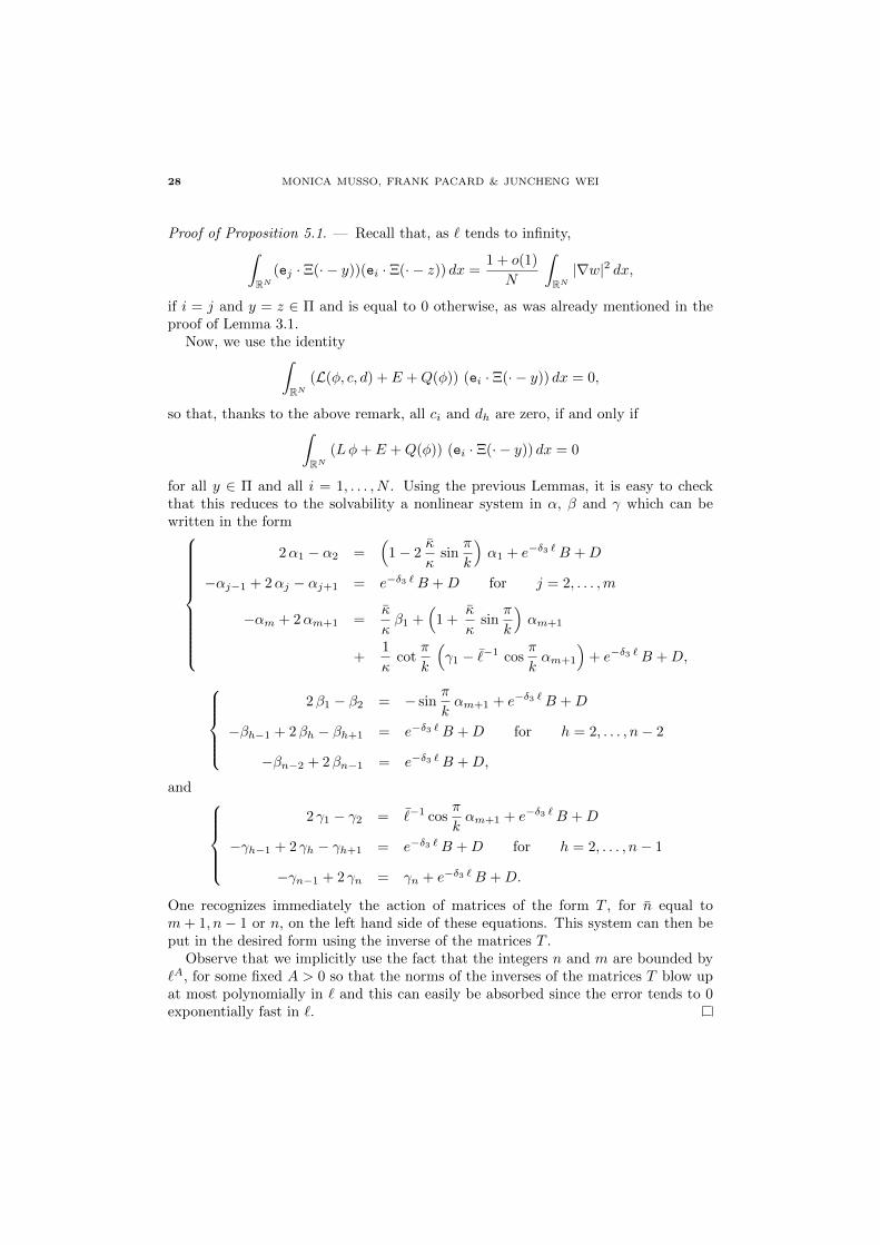
Proof of Proposition 5.1. — Recall that, as ` tends to infinity,∫RN
(ej · Ξ(· − y))(ei · Ξ(· − z)) dx =1 + o(1)
N
∫RN|∇w|2 dx,
if i = j and y = z ∈ Π and is equal to 0 otherwise, as was already mentioned in theproof of Lemma 3.1.
Now, we use the identity∫RN
(L(φ, c, d) + E +Q(φ)) (ei · Ξ(· − y)) dx = 0,
so that, thanks to the above remark, all ci and dh are zero, if and only if∫RN
(Lφ+ E +Q(φ)) (ei · Ξ(· − y)) dx = 0
for all y ∈ Π and all i = 1, . . . , N . Using the previous Lemmas, it is easy to checkthat this reduces to the solvability a nonlinear system in α, β and γ which can bewritten in the form
2α1 − α2 =(
1− 2κ
κsin
π
k
)α1 + e−δ3 `B +D
−αj−1 + 2αj − αj+1 = e−δ3 `B +D for j = 2, . . . ,m
−αm + 2αm+1 =κ
κβ1 +
(1 +
κ
κsin
π
k
)αm+1
+1
κcot
π
k
(γ1 − ¯−1 cos
π
kαm+1
)+ e−δ3 `B +D,
2β1 − β2 = − sin
π
kαm+1 + e−δ3 `B +D
−βh−1 + 2βh − βh+1 = e−δ3 `B +D for h = 2, . . . , n− 2
−βn−2 + 2βn−1 = e−δ3 `B +D,
and 2 γ1 − γ2 = ¯−1 cos
π
kαm+1 + e−δ3 `B +D
−γh−1 + 2 γh − γh+1 = e−δ3 `B +D for h = 2, . . . , n− 1
−γn−1 + 2 γn = γn + e−δ3 `B +D.
One recognizes immediately the action of matrices of the form T , for n equal tom+ 1, n− 1 or n, on the left hand side of these equations. This system can then beput in the desired form using the inverse of the matrices T .
Observe that we implicitly use the fact that the integers n and m are bounded by`A, for some fixed A > 0 so that the norms of the inverses of the matrices T blow upat most polynomially in ` and this can easily be absorbed since the error tends to 0exponentially fast in `.

FINITE-ENERGY SIGN-CHANGING SOLUTIONS 29
We now explain how (5.4) can be solved. We claim that this system is equivalentto
α = e−δ2`B +D,
β = e−δ2`B +D,
γ = e−δ2`B +D,
where δ2 > 0 and B = B(`,m, n;α, β, γ) and D = D(`,m, n;α, β, γ) satisfy the usualassumptions.
Observe that the system (5.4) is almost of the correct form. Below, we agree
that both δ2 > 0 and the nonlinear functions B = B(`,m, n;α, β, γ) and D =D(`,m, n;α, β, γ) may change from line to line but they satisfy the usual assump-tions. In fact, using the second and third equation together with the expression of S↑
and S↓ one checks that γ1, β1 and γn can be expressed in terms of αm+1 and lowerorder terms. More precisely, we get
β1 = −n− 1
nsin
π
kαm+1 + e−δ2`B +D
¯γ1 = cosπ
kαm+1 + e−δ2`B +D
¯γn = cosπ
kαm+1 + e−δ2`B +D.
Hence we get
κ
κβ1 +
1
κcot
π
kγ1 + λ2 αm+1 =
(1 +
1
n
κ
κsin
π
k
)αm+1 + e−δ2`B +D.
Introducing these in the first equation, we are left to solve a coupled system in α1
and αm+1. This system reads(
1 + 2 (m+ 1)κ
κsin
π
k
)α1 −
(1 +
1
n
κ
κsin
π
k
)αm+1 = e−δ2`B +D,
−(
1− 2κ
κsin
π
k
)α1 +
(1− 1
n(m+ 1)
κ
κsin
π
k
)αm+1 = e−δ2`B +D.
This system can be solved to be put in diagonal form provided D0, the determinantof the 2 by 2 system on the left had side, is non zero. But, we have
D0 =κ
κsin
π
k
m+ 2
n
(2n− 1− 2m sin
π
k
κ
κ
).
Using (1.12) together with (1.17), we conclude that
D0 =κ
κ2sin
π
k
m+ 2
n(2n− 1)
(`− ¯
`+O(`−2)
),
which, thanks to (1.29), is certainly bounded from below by some constant times m/`for all ` large enough. This completes the proof of the claim.
It is now straightforward to prove, using Browder’s fixed point theorem, that
30 MONICA MUSSO, FRANK PACARD & JUNCHENG WEI
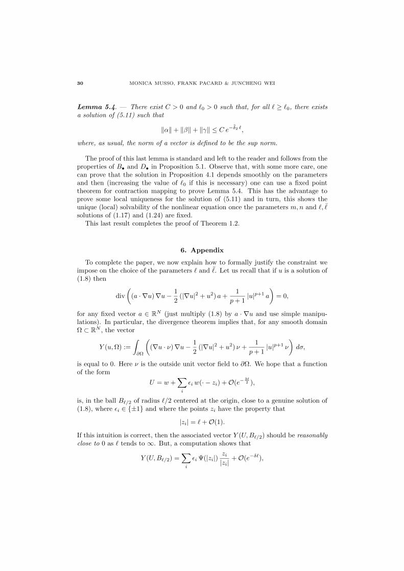
Lemma 5.4. — There exist C > 0 and `0 > 0 such that, for all ` ≥ `0, there existsa solution of (5.11) such that
‖α‖+ ‖β‖+ ‖γ‖ ≤ C e−δ2 `,
where, as usual, the norm of a vector is defined to be the sup norm.
The proof of this last lemma is standard and left to the reader and follows from theproperties of B• and D• in Proposition 5.1. Observe that, with some more care, onecan prove that the solution in Proposition 4.1 depends smoothly on the parametersand then (increasing the value of `0 if this is necessary) one can use a fixed pointtheorem for contraction mapping to prove Lemma 5.4. This has the advantage toprove some local uniqueness for the solution of (5.11) and in turn, this shows theunique (local) solvability of the nonlinear equation once the parameters m,n and `, ¯
solutions of (1.17) and (1.24) are fixed.This last result completes the proof of Theorem 1.2.
6. Appendix
To complete the paper, we now explain how to formally justify the constraint weimpose on the choice of the parameters ` and ¯. Let us recall that if u is a solution of(1.8) then
div
((a · ∇u)∇u− 1
2(|∇u|2 + u2) a+
1
p+ 1|u|p+1 a
)= 0,
for any fixed vector a ∈ RN (just multiply (1.8) by a · ∇u and use simple manipu-lations). In particular, the divergence theorem implies that, for any smooth domainΩ ⊂ RN , the vector
Y (u,Ω) :=
∫∂Ω
((∇u · ν)∇u− 1
2(|∇u|2 + u2) ν +
1
p+ 1|u|p+1 ν
)dσ,
is equal to 0. Here ν is the outside unit vector field to ∂Ω. We hope that a functionof the form
U = w +∑i
εi w(· − zi) +O(e−3`2 ),
is, in the ball B`/2 of radius `/2 centered at the origin, close to a genuine solution of(1.8), where εi ∈ ±1 and where the points zi have the property that
|zi| = `+O(1).
If this intuition is correct, then the associated vector Y (U,B`/2) should be reasonablyclose to 0 as ` tends to ∞. But, a computation shows that
Y (U,B`/2) =∑i
εi Ψ(|zi|)zi|zi|
+O(e−δ`),

FINITE-ENERGY SIGN-CHANGING SOLUTIONS 31
for some δ > 1, as ` tends to 0. Therefore, in order for the construction to besuccessful, it is reasonable to ask that∑
i
εi Ψ(|zi|)zi|zi|
= 0.
This is precisely the balancing condition we were referring to. Applying this to theapproximate solution U at the points y1 and ym+1 leads to (1.24).
References
[1] T. Bartsch and M. Willem, Infinitely many nonradial solutions of a Euclidean scalarfield equation, J. Funct. Anal. 117 (1993), 447-460.
[2] T. Bartsch and M. Willem, Infinitely many radial solutions of a semilinear ellipticproblem on RN , Arch. Rat. Mech. Anal. 124 (1993), 261-276.
[3] H. Berestycki and P.L. Lions, Nonlinear scalar field equations, I, Existence of a groundstate, Arch. Rat. Mech. Anal. 82 (1981), 313-347.
[4] H. Berestycki and P.L. Lions, Nonlinear scalar field equations, II, Arch. Rat. Mech.Anal. 82 (1981), 347-375.
[5] M. Conti, L. Merizzi and S. Terracini, Radial solutions of superlinear problems in RN ,Arch. Rat. Mech. Anal. 153 (2000), 291-316.
[6] M. del Pino, M. Kowalczyk, F. Pacard and J. Wei, The Toda system and multiple-endsolutions of autonomous planar elliptic problems, J. Functional Analysis, 258, (2010)458-503.
[7] B. Gidas, W. M. Ni and L. Nirenberg, Symmetry of positive solutions of nonlinearelliptic equations in Rn, Mathematical Analysis and Applications, Part A, Adv. Math.Suppl. Studies Vol. 7A, 369-402, Academic Press, New York, 1981.
[8] M. Jleli and F. Pacard, An end-to-end construction for compact constant mean curvaturesurfaces. Pacific Journal of Maths, 221, no. 1, (2005) 81-108.
[9] N. Kapouleas, Compact constant mean curvature surfaces in Euclidean three-space. J.Differential Geom. 33 (1991), no. 3, 683-715.
[10] M. K. Kwong, Uniquness of positive solutions of ∆u−u+up = 0 in RN , Arch. RationalMech. Anal. 105, (1991), 243-266.
[11] M. K. Kwong and L. Zhang, Uniqueness of the positive solution of ∆u + f(u) = 0 inan annulus, Diff. Int. Eqns. 4 , no. 3, (1991), 583-599.
[12] F. H. Lin, W. M. Ni and J.C. Wei, On the number of interior peak solutions for asingularly perturbed Neumann problem, Comm. Pure Appl. Math. 60 (2007), 252-281.
[13] S. Lorca and P. Ubilla, Symmetric and nonsymmetric solutions for an elliptic equationon RN , Nonlinear Anal. 58, (2004), 961-968.
[14] A. Malchiodi. Some new entire solutions of semilinear elliptic equations in RN , Adv.Math. 221, no. 6, (2009), 1843-1909.
[15] W. M. Ni and I. Takagi, Locating the peaks of least-energy solutions to a semilinearNeumann problem, Duke Math. J. 70, no. 2, (1993), 247-281.
[16] M. Struwe, Multiple solutions of differential equations without the Palais-Smale condi-tion, Math. Ann. 261, (1982), 399-412.
[17] J. C. Wei and S. Yan, Infinitely many positive solutions for the nonlinear Schrodingerequations in RN , J. Functional Analysis, 258, (2010), 3048-3081.

32 MONICA MUSSO, FRANK PACARD & JUNCHENG WEI
Monica Musso, Departamento de Matematica, Pontificia Universidad Catolica de Chile, Avda.
Vicuna Mackenna 4860, Macul, Chile and Dipartimento di Matematica, Politecnico di Torino,Corso Duca degli Abruzzi, 24- 10129 Torino, Italy. Email : [email protected]
Frank Pacard, [email protected], Centre de Mathematiques Laurent Schwartz,
Ecole Polytechnique, 91128 Palaiseau, France and Institut Universitaire de France. Email:
Juncheng Wei, J. Wei - Department of Mathematics, The Chinese University of Hong Kong,Shatin, Hong Kong. Email: [email protected]